arX

iv:0

708.

1236

v1 [

gr-q

c] 9

Aug

200

7

Flipped spinfoam vertex and loop gravity

Jonathan Engle, Roberto Pereira and Carlo Rovelli

CPT∗, CNRS Case 907, Universite de la Mediterranee, F-13288 Marseille, EU

February 1, 2008

Abstract

We introduce a vertex amplitude for 4d loop quantum gravity. We derive it from a conventionalquantization of a Regge discretization of euclidean general relativity. This yields a spinfoam sumthat corrects some difficulties of the Barrett-Crane theory. The second class simplicity constraintsare imposed weakly, and not strongly as in Barrett-Crane theory. Thanks to a flip in the quantumalgebra, the boundary states turn out to match those of SO(3) loop quantum gravity – the two canbe identified as eigenstates of the same physical quantities – providing a solution to the problem ofconnecting the covariant SO(4) spinfoam formalism with the canonical SO(3) spin-network one.The vertex amplitude is SO(3) and SO(4)-covariant. It rectifies the triviality of the intertwinerdependence of the Barrett-Crane vertex, which is responsible for its failure to yield the correctpropagator tensorial structure. The construction provides also an independent derivation of thekinematics of loop quantum gravity and of the result that geometry is quantized.

1 Introduction

While the kinematics of loop quantum gravity (LQG) [1] is rather well understood [2, 3], its dynamics

is not understood as cleanly. Dynamics is studied along two lines: hamiltonian [4] or covariant. Thekey object that defines the dynamics in the covariant language is the vertex amplitude, like the vertexamplitude ∼∼s< = eγµδ(p1 + p2 + k) that defines the dynamics of perturbative QED. What is thevertex of LQG?

The spinfoam formalism [5, 6, 7, 8, 9] can be viewed as a tool for answering this question: thespinfoam vertex plays a role similar to the vertices of Feynman’s covariant quantum field theory.This picture is nicely implemented in three dimensions (3d) by the Ponzano-Regge model [10], whoseboundary states match those of LQG [11] and whose vertex amplitude can be obtained as a matrixelement of the hamiltonian of 3d LQG [12]. But the picture has never been fully implemented in4d. The best studied model in the 4d euclidean context is the Barrett-Crane (BC) theory [8], whichis based on the vertex amplitude introduced by Barrett and Crane [7]. This is simple and elegant,has remarkable finiteness properties [13], but the suspicion that something is wrong with it has longbeen agitated. Its boundary state space is similar to, but does not exactly match, that of LQG; inparticular the volume operator is ill-defined. Worse, recent results [14] indicate that it appear to failto yield the correct tensorial structure of the graviton propagator in the low-energy limit [15].

It is then natural to try to correct the BC model [16, 17, 18]. The difficulties are all related to thefact that in the BC model the intertwiner quantum numbers are fully constrained. This follows from

∗Unite mixte de recherche (UMR 6207) du CNRS et des Universites de Provence (Aix-Marseille I), de la Meditarranee(Aix-Marseille II) et du Sud (Toulon-Var); laboratoire affilie a la FRUMAM (FR 2291).

1

the fact that the simplicity constraints are imposed as strong operator equations (Cnψ = 0). However,these constraints are second class and it is well known that imposing second class constraints stronglymay lead to the incorrect elimination of physical degrees of freedom [19]. In this paper we show thatthe simplicity constraints can be imposed weakly (〈φCn ψ〉 = 0), and that the resulting theory hasremarkable features. First, its boundary quantum state space matches exactly the one of SO(3) LQG:no degrees of freedom are lost. Second, as the degrees of freedom missing in BC are recovered, thevertex may yield the correct low-energy n-point functions. Third, the vertex can be seen as a vertexover SO(3) spin networks or SO(4) spin networks, and is both SO(3) and SO(4) covariant.

These results have been anticipated in a letter [20]. Here we derive them via a proper quantizationof a discretization of euclidean general relativity (GR). Indeed, although spinfoam models have beenderived in a number of different manners [6, 7, 8, 21], most derivations involve peculiar proceduresor intuitive and ad hoc steps. It is hard to find a proper derivation of a spinfoam model from theclassical field theory, which follows well-tested quantization procedures. Here we try to fill this gap.

From the experience with QCD, one can derive the persuasion that a nontrivial quantum fieldtheory should be related to a natural lattice discretization of the corresponding classical field theory[22]. This persuasion is reinforced by the LQG prediction of an actual physical discretization ofspacetime. Here, we reconstruct the basis of the euclidean spinfoam formalism as a proper quantizationof a lattice discretization of GR. Conventional lattice formalisms as the ones used in QCD are not verynatural for GR, since they presuppose a background metric. Regge has found a particularly naturalway to discretize GR on a lattice [23], known as Regge calculus. Quantization of Regge calculus hasbeen considered in the past [24] and its relation to spinfoam theory has been pointed out (see [25]and references therein). Here we express Regge calculus in terms of the elementary fields used inthe loop and spinfoam approach, namely holonomies and the Plebanski two-form, and we study thequantization of the resulting discrete theory (on lattice derivations of loop gravity, see [6, 27, 28]).

The technical ingredient that allows a nontrivial intertwiner state space to emerge can be inter-preted as a “flip” of the SO(4) algebra, namely an opposite choice of sign in one of its two SU(2)factors. The possibility and the relevance of a “flipped” symplectic structure was noticed by Baezand Barrett in [26] (where they attribute the observation to Jose-Antonio Zapata) and by Montesinos[29]. Montesinos, in particular, has discussed the classical indeterminacy of the symplectic structurein detail. The flip can be viewed as the equivalent of the Ashtekar “trick”, which yields a connectionas phase space variable. The SO(4) generators turn out to directly correspond to the bivectors asso-ciated to the Regge triangles, rather than to their dual. Using this, we find a nontrivial subspace ofthe SO(4) intertwiner space, which corresponds to closed tetrahedra and maps naturally to an SO(3)intertwiner space.

This path leads to a quantum theory that appears to improve several aspects of the better knownspinfoam models. In particular: (i) the geometrical interpretation for all the variables becomes fullytransparent; (ii) the boundary states fully capture the gravitational field boundary variables; and(iii) correspond precisely to the spin network states of LQG. The identification is not arbitrary: theboundary states of the model are precisely eigenstates of the same quantities as the correspondingLQG states. This last result provides a solution to the long-standing difficulty of connecting thecovariant SO(4) spinfoam formalism with the SO(3) canonical LQG one. It also provides a novelindependent derivation of the LQG kinematics, and, in particular, of the quantization of area andvolume. Finally, (iv) the vertex of the theory is similar to, but different from, the BC vertex, leadingto a dynamics that might be better behaved in the low-energy limit.

The paper is organized pedagogically and is largely self contained. Section 2 reviews backgroundmaterial: properties of SO(4) and its selfdual/anti-selfdual split, and the definition of the fields andthe formulation of classical GR as a constrained Plebanski theory. In section 3 we discretize thetheory on a fixed triangulation of spacetime. We do so simply by taking standard Regge calculus andre-expressing it in terms of the (discretized) Plebanski two-form. The resulting theory is governed

2

by the geometry of a 4-simplex, which we illustrate in detail. All basic relations among the variableshave a simple interpretation in these terms. The 10 components of the metric tensor gab in a point(or in a cell) can be interpreted as a way to code the 10 variables determining the shape of the cell.In particular, the norms of the discretized B fields on the faces are their areas and the scalar producton adjacent triangles codes the angle between the triangles. While these “angles” and “areas” areindependent in BF theory, they are related if they derive from a common metric, namely in GR.In Section 4 we study the quantization of the system. We explain the difficulties of imposing theconstraints strongly, study the weak constraints and write their solution. Finally we construct thevertex amplitude.

We work in the euclidean signature, and on a fixed triangulation. The issues raised by recoveringtriangulation independence and the relation with the Lorentzian–signature theory will be discussedelsewhere.

2 Preliminaries: Plebanski two-form and structure of SO(4)

Riemannian general relativity (GR) is defined by a riemannian metric gab(x), where a, b = 1, 2, 3, 4and the Einstein-Hilbert action

S[g] =

∫ √g R =

∫ √g gabRab. (1)

where gab is the inverse, g the determinant, and Rab the Ricci curvature of gab. A good number ofreasons, such as for instance the fact that this metric formulation is incompatible with the couplingwith fermions, suggest to use the tetrad field ea

I (x), I = 1, 2, 3, 0, (the value 0 instead of 4 is for laterconvenience and does not indicate a Lorentzian metric) or its inverse, namely the tetrad one-form fieldeI(x) = eI

a(x)dxa, to describe the gravitational field. This is related to the metric by eIae

Ib = gab. Sum

over repeated indices is understood, and the up or down position of the I indices is irrelevant. Thespin connection of the tetrad field is an SO(4) connection ωIJ [e] satisfying the torsion-free condition

DeI = deI + ωIJ [e] ∧ eJ = 0. (2)

The action (1) can be rewritten as a function of eI in the form

S[e] =

∫

(det e) eaIe

bJF

IJab [ω[e]] =

1

2

∫

ǫIJKL eI ∧ eJ ∧ FKL[ω[e]] (3)

where F [ω] is the curvature of ω. Alternatively, GR can be defined in first order form in terms ofindependent variables ωIJ and eI , by the action

S[e, ω] =1

2

∫

ǫIJKL eI ∧ eJ ∧ FKL[ω]. (4)

In this case, (2) is obtained as the equation of motion for ω.

2.1 Plebanski two-form and simplicity constraints

At the basis of the spinfoam formalism is the use of the Plebanski two-form ΣIJ ≡ 12ΣIJ

ab dxa ∧ dxb,defined as

ΣIJ = eI ∧ eJ . (5)

or its dual, usually called BIJ ≡ 12B

IJab dxa ∧ dxb for a reason that will be clear in a moment, defined

as

BIJ =1

2ǫIJ

KL ΣKL =1

2ǫIJ

KL eK ∧ eL (6)

3

We use the following notation for two-index objects: a scalar product: A · B ≡ AIJBIJ ; a norm:|B|2 ≡ B · B, and the duality operation (∗B)IJ = 1

2ǫIJ

KL BKL. So that, in particular, ∗B · B =12ǫIJKL BIJBKL. Thus we write (6) in the form

B = ∗Σ = ∗(eI ∧ eJ) (7)

The geometrical interpretation of the Plebanski two-form (or the B two-form) is captured by thefollowing. Observe that

|Σab|2 = |Bab|2 = gaagbb − gabgab ≡ 2A2ab (8)

andΣab · Σac = Bab ·Bac = gaagbc − gabgac ≡ 2Jaabc (9)

The quantity Aab gives the area element Aabdxadyb of the infinitesimal surface dxadyb. Therefore we

can write∫

S

|Σ| =

∫

S

|B| ≡∫

S

|Σab| dxadyb =√

2 ×Area(S) (10)

The quantity Jaabc is the related to the angle θaabc between the surface elements dxadyb and dxadzc.In fact, if we take the scalar product of the normals of these two surface elements (in the 3-space theyspan), we obtain (without writing the infinitesimals vectors)

AabAac cos θaa bc = gef (ǫeghδgaδ

hb )(ǫfghδ

gaδ

hc ) = gaagbc − gabgac = Jaabc. (11)

Finally, the 4-form

V ≡ 1

4!ǫIJKLΣIJ ∧ ΣKL =

1

4!ǫIJKLB

IJ ∧BKL (12)

is easily seen to be (proportional to) the volume element dV =√g d4x. Intuitively, describing the

geometry in terms of Σ rather than gab is using as elementary variable areas and angles rather thanlength and angles.

Using the Plebanski field, the action can be written in the BF-like form

S[e, ω] =1

2

∫

ǫIJKL ΣIJ [e] ∧ FKL[ω] =

∫

BIJ [e] ∧ F IJ [ω]. (13)

The reason this action defines GR and not BF theory is that the independent variable to vary is thetetrad e, not the two-form B. While the BF field equations are obtained by varying the action (13)under arbitrary variations of B (and ω), GR is defined by varying this action under the variationsthat respect the form (6) of the field B. This condition can be expressed as a constraint equation forΣ:

ΣIJ ∧ ΣKL = V ǫIJKL (14)

Equivalently ,∗Σab · Σcd = 2V ǫabcd. (15)

where V = 14! V ǫabcddx

a ∧ ... ∧ dxd. This system of constraint can be decomposed in three parts:

a) ∗Σab · Σab = 0 , (16)

b) ∗Σab · Σac = 0 , (17)

c) ∗Σab · Σcd = ±2V . (18)

where the indices abcd are all different, and the sign in the last equation is determined by the signof their permutation. Equivalently, the B field satisfies these same equations. These three constraintplay an important role in the following. They are called the simplicity constraints. GR can be writtenas an SO(4) BF theory whose B field satisfies the simplicity constraints (16-17-18).

4

2.2 Selfdual structure of SO(4)

In this section we recall some elementary facts about SO(4) and we make an observation about itsrepresentations that plays a role in the following.

The group SO(4) is locally isomorphic to the product of two subgroups, each loc. isomorphicto SU(2): SO(4) ∼ (SU(2)+ × SU(2)−) /Z2. That is, we can write each U ∈ SO(4) in the formU = (g+, g−) where g+ ∈ SU(2)+ and g− ∈ SU(2)− and UU ′ = (g+g

′+, g−g

′−). This is clearly seen

looking at its algebra so(4), which is the linear sum of two commuting su(2) algebras. Explicitly, letJIJ be the generators of so(4). Define the selfdual and anti-selfdual generators J± := ∗J ± J, thatsatisfy J± = ±∗ J±. Then it is immediate to see that [J+, J−] = 0. The J+ span a three dimensionalsubalgebra su(2)+ of so(4), and the J− span a three dimensional subalgebra su(2)− of so(4), bothisomorphic to su(2).

It is convenient to choose a basis in su(2)+ and in su(2)−. For this, choose a unit norm vector n inR4, and three other vectors vi, i = 1, 2, 3 forming, together with n, an orthonormal basis, for instancevI

i = δIi , and define

J i± =

1

2(∗J ± J)IJ vI

i nJ (19)

The su(2) structure is then easy to see, since [J i±, J

j±] = ǫijkJ

k±. In particular, we can choose n =

(0, 0, 0, 1), and vIi = δI

i , and we have

J i± = −1

4ǫijkJ

jk ± 1

2J i0. (20)

Notice that in choosing this basis we have broken SO(4) invariance. In fact, the split so(4) =su(2)+ ⊕ su(2)− is canonical, but there is no canonical isomorphism between su(2)+ and su(2)− orbetween SU(2)+ and SU(2)−. One such isomorphism Gn : SU(2)+ → SU(2)− is picked up, forinstance, by choosing the vector n. It sends g+ to g−, where the element (g+, g−) of SO(4) leavesn invariant. This isomorphism defines a notion of diagonal elements of the so(4) algebra: the onesof the form aiJ

i+ + aiJ

i−. Exponentiating these, we get the diagonal elements of the SO(4) group,

which we can write as U = (g, g). These diagonal elements form an SU(2) subgroup of SO(4), whichis not canonical: it depends on n. It is the subgroup of SO(4) that leaves the vector n invariant.If we consider the 3d surface (“space”) orthogonal to n, the diagonal part of SO(4) is (the doublecovering of) the SO(3) group of the (“spatial”) rotations of this space; we denote it SO(3)n ⊂ SO(4).Borrowing from the Lorentzian terminology, we can call “boost” a change of n. Its effect is to rotatethe ± bases relative to one another.

Notice that for any two-index quantity BIJ ,

1

4B · B = Bi

+Bi+ +Bi

−Bi−, (21)

while1

4∗B ·B = Bi

+Bi+ − Bi

−Bi−. (22)

This split is independent from n, as the norms are not affected by a rotation of the basis. In particular,C = 1

4J · J and C = 14∗J · J are the scalar and pseudo-scalar quadratic Casimirs of so(4). They

are, respectively, the sum and the difference of the quadratic Casimirs of su(2)+ and su(2)−. Therepresentations of the universal cover of SO(4), the group Spin(4) ∼ SU(2) × SU(2) are labelled bytwo half integers (j+, j−). The representations of SO(4) form the subset of these for which j+ + j− isinteger. The representations satisfying j+ = j−, which clearly belong to this subset, are called simple:they play a major role in the BC theory as well as in the quantization below.

The following observation plays a major role in section 4.2. Consider a simple representation(j, j). This is also a representation of the subgroup SO(3)n ⊂ SO(4), but a reducible one. Clearly, it

5

transforms in the representation j ⊗ j, where j indicates the usual spin j representation of SU(2). Ifwe decompose it into irreducible representations of SO(3)n, we have

(j, j) → j ⊗ j = 0 ⊕ 1 ⊕ ...⊕ (2j − 1) ⊕ 2j. (23)

The value of C4 in this representation is 2(j(j + 1)). Consider the value that the Casimir C3 of thesubgroup SO(3)n takes on the lowest and highest-spin representations. C3 vanishes on the spin-0representation. On the spin-2j representation, it has the value C3 = 2j(2j + 1), which is related toC4 by

√

C3 + 1/4 −√

2C4 + 1 + 1/2 = 0 (24)

and in the large j limit byC3 = 2C4, (25)

that is, if we have chosen n = (0, 0, 0, 1),

JIJJIJ = J ijJij + 2J0iJ0i, (26)

which implies J0i = 0. Therefore, the spin-zero and the spin-2j components of the simple SO(4)representation (j, j) are characterized respectively by

spin 0 : J ij = 0,

spin 2j : J i0 = 0 (27)

in the “classical” large-j limit.

3 Regge discretization

We now approximate euclidean GR by means of a discrete lattice theory. A very natural way ofdoing so is Regge calculus [23]. The idea of Regge calculus is the following. The object described byeuclidean GR is a Riemannian manifold (M,dM ), whereM is a differential manifold and dM its metric.A Riemannian manifold can be approximated by means of a piecewise flat manifold (∆, d∆), formedby flat (metric) simplices (triangles in 2d, tetrahedra in 3d, 4-simplices in 4d...) glued together in sucha way that the geometry of their shared boundaries matches. Here ∆ is the abstract triangulation andd∆ is its metric, which is determined by the size of the individual simplices. For instance, a curved2d surface can be approximated by a surface obtained by gluing together flat triangles along theirsides: curvature is then concentrated on the points where triangles meet, possibly forming “the topof a hill”. With a sufficient number N of simplices, we can approximate sufficiently well any given(compact) Riemannian manifold (M,dM ), with a Regge triangulation (∆, d∆).1

If we fix the abstract triangulation ∆ and we vary d∆, namely the size of the individual n-simplices, then we can approximate to a certain degree a subset of GR fields. Therefore by fixing ∆we capture a subspace of the full set of all possible gravitational fields. Thus, over a fixed ∆ we candefine an approximation of GR, in a manner analogous to the way a given Wilson lattice defines anapproximation to Yang-Mills field theory, or the approximation of a partial differential equation withfinite–differences defines a discretization of the equation. Therefore the Regge theory over a fixed ∆defines a cut-off version of GR.

1For instance, in the sense that the two can be mapped into each other, P : M → ∆, in such a way that thedifference between the distances between any two points, dM (x, y)− d∆(P (x), P (y)), can be made arbitrary small withN sufficiently large.

6

It is important to notice, however, that the Regge cut-off is neither ultraviolet nor infrared. This issharp contrast with the case of lattice QCD. In lattice QCD, the number N of elementary cells of thelattice defines an infrared cut-off: long wavelength degrees of freedom are recovered by increasing N .On the other hand, the physical size a of the individual cells enters the action of the theory, and shortwavelength degrees of freedom are recovered in lattice QCD by decreasing a. Hence a is ultravioletcut-off. In Regge GR, on the contrary, there is no fixed background size of the cells that enters theaction. A fixed ∆ can carry both a very large or a very small geometry. The cut-off implemented by∆ is therefore of a different nature than the one of lattice QCD. It is not difficult to see that it isa cut-off in the ratio between the smallest allowed wavelength and the overall size of the spacetimeregion considered. Thus, fixing ∆ is equivalent to cutting-off the degrees of freedom of GR that havemuch smaller wavelength than the arbitrary size L of the region one considers. Since (as we shall see,and as implied by LQG) the quantum theory has no degrees of freedom below the Planck scale, itfollows that a Regge approximation is good for L small, and it is a low-energy approximation for Llarge.2

Consider a 4d triangulation. This is formed by oriented 4-simplices, tetrahedra, triangles, segmentsand points. We call v, t and f respectively the 4-simplices, the tetrahedra and the triangles of thetriangulation decomposition. The choice of the letters v and f is dictated by the fact that in thedual-complex, to which we will later shift, 4-simplices are dual to vertices, and triangles are dualto faces.3 The metric, we recall, is flat within each 4-simplex v. All the tetrahedra, triangles andsegments are flat (and, respectively, straight). The geometry induced on a given tetrahedron fromthe geometry of the two adjacent 4-simplices is the same. This structure will allow us to take thegeometry of the tetrahedra as the fundamental dynamical object, and interpret the constraints impliedby the fact that five tetrahedra fit into a single four-simplex as the expression of the dynamics. It isthis peculiar perspective that makes the construction below possible.

In d dimensions, a d − 2 simplex is surrounded by a cyclic sequence of d-simplices, separated bythe d− 1 simplices that meet at the d− 2 simplex. This cyclic sequence is called the link of the d− 2simplex. For instance, in dimension 2, a point is surrounded by a link of triangles, separated by theedges that meet at the point; in dimension 3, it is an edge which is surrounded by a link of tetrahedra,separated by the triangles that meet at the edge; in dimension 4, which is the case that concerns us,a triangle f is surrounded by a link of 4-simplices v1, ..., vn, separated by the tetrahedra that meet atthe triangle f .

In Regge calculus, curvature is concentrated on the d − 2 simplices. In dimension 4, curvature istherefore concentrated on the triangles f . It is generated by the fact that the sum of the dihedralangles of the 4-simplices in the link around the triangle may be different from 2π. We can alwayschoose Cartesian coordinates covering one 4-simplex, or two adjacent 4-simplices; but in general thereare no continuous Cartesian coordinates covering the region formed by all the 4-simplices in the linkaround a triangle.

The variables used by Regge to describe the geometry d∆ of the triangulation ∆ are given by theset of the lengths of all the segments of the triangulation. Here we make a different choice of variables,which matches more closely what happens in the spinfoam formalism and in loop gravity.

Consider one tetrahedron t in the triangulation. Choose a Cartesian coordinate system xa covering

2Since the expansion parameter λ used in group field theory [30] is equivalent to the number of cells in Regge calculus,this discussion clarifies also the physical meaning of the group field theory λ expansion.

3For coherence, we should also call e the tetrahedra, which are dual to the edges of the dual complex; this is indeedthe common convention [3]. But in the present context this would generate confusion with the notation for the tetrad.We will shift to the e notation for edges only later on, in the quantum theory part.

7

t’

t

f

U1

U2

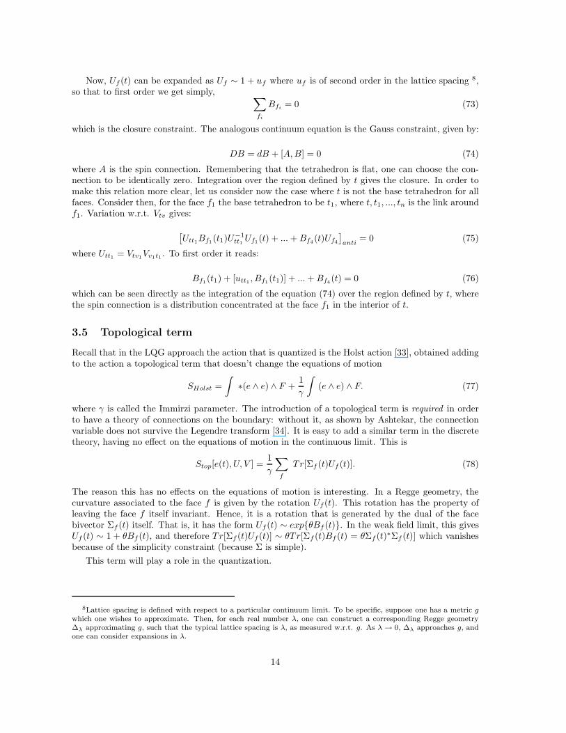
Figure 1: The link of the face f , in grey, and the two group elements associated to a couple oftetrahedra t and t′ in the link.

the tetrahedron. Choose an orthonormal basis

e(t) = eIa(t) vI dx

a (28)

for each such tetrahedron t. Here vI is a basis in R4, chosen once and for all. This quantity of coursetransforms covariantly under a change coordinate system xa, therefore it is intrinsically defined as aone-form with values in R4, associated to the tetrahedron. This will be our first variable, giving adiscretized approximation of the gravitational field.

Consider the five tetrahedra tA, A = 1, ...5 that bound a single simplex v. The five variablese(tA) are not independent, because the simplex is flat. Since the simplex is flat, we can alwayschoose a common Cartesian coordinate system xa for the entire v. Let e(v) = eI

a(v) vI dxa denote an

orthonormal basis describing the geometry in v. Then each e(tA) must be related to e(v) by an SO(4)rotation in R4. That is there must exist five SO(4) matrices VvtA

such that

e(v)Ia = (VvtA

)IJ e

Ja (tA) (29)

in the common coordinate patch. One can also define the transformation from one tetrahedron to theother:

e(tA) = UtAtB(v)e(tB) (30)

The later are of course constrained by the former:

UtAtB(v) = VtAv VvtB

(31)

where VtAv ≡ V −1vtA

. Now consider two tetrahedra t and t′ sharing a face but not necessarily at the samefour simplex and define as before the SO(4) transformation between the two Utt′ . Remember thatone can choose the same coordinate system for an open chain of four simplices linking two tetrahedraaround the face they share. This constrains Utt′ to be of the form:

Utt′ = Vtv1... Vvnt′ (32)

where v1 ... vn is the (open) chain of 4-simplices between t and t′ around their common face. Nowone must be cautious. For two arbitrary tetrahedra sharing a face in the interior of the discretization,there are two such chains (see Figure 1) To resolve this ambiguity, we make use of the orientationof the face f : this orientation gives a notion of clockwise and counterclockwise around the link. Wechoose the convention that Utt′ denote the holonomy around the chain in the clockwise direction,starting at t′ and ending at t. (For f on the boundary, or when one is considering a single 4-simplex,of course the orientation of f need not be used to resolve this ambiguity.)

8

The arbitrariness in the choice of the orthonormal basis at each tetrahedron is reflected in thelocal SO(4) gauge transformations

e(t) → Λ(t) e(t), (33)

e(v) → Λ(v) e(v), (34)

Vvt → Λ(v) Vvt Λ(t)−1, (35)

Utt′ → Λ(t) Utt′ Λ(t′)−1, (36)

where Λ(t),Λ(v) ∈ SO(4) are the gauge parameters associated with the choice of basis in tetrahedraand vertices respectively.

In each tetrahedron t, consider the bivector two-form

Σ(t) = e(t) ∧ e(t). (37)

and its dualB(t) = ∗Σ(t). (38)

In components, this is B(t) = 12B

IJab (t)vIvJdx

a ∧ dxb where

BIJab (t) = ǫIJ

KL eKa (t)eL

b (t). (39)

Now, consider a tetrahedron t and a triangle f in its boundary. Associate a bivector Σf (t) to thetriangle f , as follows. Σf (t) is defined as the surface integral of the two-form Σ(t) over the triangle

Σf (t) =

∫

f

Σ(t). (40)

This is the geometrical bivector naturally associated to the (oriented) triangle, in the frame asso-ciated to the tetrahedron t. Its dual bivector is Bf (t) = ∗Σf (t). A single triangle f belongsto (the boundary of) the several tetrahedra t1, t2, t3, ... that are around its link. The bivectorsΣIJ

f (t1),ΣIJf (t2),Σ

IJf (t3), ... are different, because they represent the triangle in the internal frames

associated to distinct tetrahedra. But they are of course related by

ΣIJf (t1) = Ut1t2

IK(v12) Ut1t2

JL(v12) ΣKL

f (t2). (41)

Notice that if the tetrad is Euclidean eIa(t) = δI

a and the triangle is in the (1,2) plane, the onlynon-vanishing components of ΣIJ

f (t) are Σ12f (t) = −Σ21

f (t), while the only non-vanishing components

of BIJf (t) are B30

f (t) = −B03f (t). More in general, if the normal of the tetrahedron is nI , then for all

the faces f of the tetrahedron t we have

ǫIJKL nJ BKLf (t) = 0, (42)

nI ΣIJf (t) = 0. (43)

In particular, if we choose a gauge where nI = (0, 0, 0, 1), we have

Bijf (t) = 0, (44)

Σi0f (t) = 0. (45)

The quantities ΣIJf (t) and Vvt can be taken as a discretization of the continuous gravitational fields

ΣIJ and ωIJ that define GR in the Plebanski formalism.

9

3.1 Constraints on Σ

Since our aim is to promote ΣIJf (t) to an independent variable, let us study the constraints it satisfies.

It is immediate to see that the four bivectors ΣIJf1

(t), ...,ΣIJf4

(t) associated to the four faces of a singletetrahedron satisfy the closure relation

ΣIJf1

(t) + ΣIJf2

(t) + ΣIJf3

(t) + ΣIJf4

(t) = 0. (46)

Since the two-form ΣIJ(t) is defined in terms of a tetrad field, it satisfies the relation (15), or,equivalently, (16,17,18). Multiplying these relations by the coordinate bivectors representing triangles,gives the following relations. For each triangle f , we have

∗ Σf (t) · Σf (t) = 0. (47)

For each couple of adjacent triangles f, f ′, we have

∗ Σf (t) · Σf ′(t) = 0. (48)

We call these two constraints the diagonal and off-diagonal simplicity constraints, respectively.

The last constraint, for f and f ′ in the same four simplex sharing just a point, is a little subtler.It is

∗ Σf (v) · Σf ′(v) = ±12V (v). (49)

where V (v) is the four volume of the simplex and the sign depends on relative face orientation [21]. Ofcourse the volume in the last formula is irrelevant. What this equation tells us is that the volume isthe same when computed with different choices of pairs of faces in the same four simplex. Now, usingthe transformation law for the bivectors (41) one can write it with tetrads defined on tetrahedra:

∗ Σf (t) ·(

Utt′(v)Σf ′(t′)U−1tt′ (v)

)

= ±12V (v). (50)

One can show that if (31) is satisfied and the first set of constraints (46,47,48) is satisfied then (49)or, equivalently, (50) is satisfied automatically.

Let’s count the degrees of freedom for each four simplex, as a check. We start with the 60 degreesof freedom of the bivectors, 6 for each face. The constraint (46) imposes 24 independent equations.The number of independent equations of the type (47) are 10, and finally the constraints of the type(48) contribute 10 independent equations. The last constraint is implicitly imposed when we considerthe tetrahedra to belong to the same four simplex. We are left with the 60 − (24 + 10 + 10) = 16degrees of freedom of the tetrad e(v).

There is however some additional discrete degeneracy. The set of constraints (46,47,48) has twoclasses of solutions (see appendix B):

ΣIJf1

= 2e[I2 e

J]3 and cyclically. (51)

andΣIJ

f1= ǫIK

KLeK2 e

L3 and cyclically. (52)

These two sectors of Plebanski theory are well known in the literature (see [5],[21]); they correspondto the fact, remarked above, that both Σ and B satisfy the same equations (46,47,48). Because of thedouble solution (51) and (52), these constraints do not determine Σ uniquely.

However, we can give the off-diagonal simplicity constraints a different and slightly stronger form,which fixes this degeneracy, and which will play a role below. We can replace the off-diagonal simplicityconstraints with the following requirement: that for each tetrahedron t there exist a covariant vectornI such that (43) holds for all the faces f of the tetrahedron t. It is immediate to see that this impliesthe off-diagonal simplicity constraints, and that it is implied by the physical solution (51) of theseconstraints. Equivalently, we require that there is a gauge in which (45) holds. The geometry of thisrequirement is transparent: nI is the normal to the tetrahedron t in four dimensions, and (43), or(45), require that the faces of the tetrahedron are all confined to the 3d hyperplane normal to nI .

10

3.2 Relation with geometry

How do we read out the geometry of the riemannian manifold, from the variables defined? First, it iseasy to see that the area of a triangle f is, up to a constant factor, the norm of its associated bivector:

√2Af = |Σf (t)| (53)

Notice that the l.h.s. is independent of t. This is consistent because the relation between ΣIJf (t) and

ΣIJf (t′) is an SO(4) transformation, whence the norm is invariant, |Σf (t)| = |Σf (t′)|. This shows that

the definitions chosen are consistent with a characteristic requirement of a Regge triangulation: theboundaries of the flat 4-simplices match, and in particular the area of a triangle computed from anyside is the same. Of course, it follows that the same is true for the volume of each tetrahedron.

Given two triangles f and f ′ in the same tetrahedron t, there is a dihedral angle θff ′ between thetwo. This angle can be obtained from the product of the normals

Jff ′ := AfAf ′ cos θff ′ = Σf (t) · Σf ′(t)/2. (54)

These are also SO(4) invariant, hence well defined independently from the tetrahedron. The twogauge invariant quantities Af and Jff ′ characterize the geometry entirely. Notice that we can viewthe area as the “diagonal” part of Jff ′ and write A2

f = Jff .

It is important to notice that, as mentioned in the previous section, the area is also (the squareroot of) the norm of its associated selfdual, or, equivalently, antiselfdual bivector:

Af = 2√

+Σif (t)+Σi

f (t) = 2√

−Σif (t)−Σi

f (t). (55)

These equalities are assured by the simplicity constraints on Σf . Similarly,

Jff ′ = 4+Σif (t)+Σi

f ′(t) = 4−Σif (t)−Σi

f ′(t), (56)

Again, these equalities follow from the simplicity constraints.

There exist a number of relations among the quantities Jff ′ within a single 4-simplex.4 Only 10 ofthese quantities can be independent, because the geometry of a 4-simplex is determined by 10 numbers.In particular, all angles must be given functions Jff ′(Af ) of the 10 areas (up to degeneracies). Explicitknowledge of the form of these functions would be quite useful in quantum gravity.

Finally, consider now a triangle f . Let t1, t2, ..., tn be the set of the tetrahedra in the link aroundf and v12, v23, ..., vn1 be the corresponding set of simplices in this link, where t2 bounds v12 and v23and so on cyclically. In general, if we parallel transport e(t) across simplices around a triangle, usingUtt′ , we come back rotated, because of the curvature at the triangle (the analog of a parallel transportaround the tip of a pyramid in 2d.) In other words, we can always gauge transform eI

a(t) to δIa within

a single cartesian coordinate patch, but in general there is no cartesian coordinate patch around aface. We define

Uf (t1) ≡ Vt1v12Vv12t2 ... Vtnvn1

Vvn1t1 (57)

or, equivalentlyUf (t1) ≡ Ut1t2(v12) ... Utnt1(vn1), (58)

the product of the rotation matrices obtained turning along the link of the triangle f , beginning withthe tetrahedron t1. The rotation matrix Uf (t1) then represents the SO(4) curvature associated to thetriangle f , written in the t1-frame.

4As a discussion of these relations does not seem to appear elsewhere in the literature, we have here included anappendix on them (A).

11

3.3 Dynamics

The last step before attacking the quantization of the model is to write the discretized action. Takethe e(t) as independent variables so that Σf (t) = e(t)∧e(t). In analogy with Regge calculus we definethe action to be

Sbulk[e(t), U, V ] =1

2

∑

f

Tr[Bf (t)Uf (t)] +∑

v

∑

f⊂v

Tr[λvfUtt′(v) Vt′v Vvt]. (59)

where we recall that B = ∗Σ. The first sum is over all faces in the interior of the discretization andUf (t) is defined as in (58), where t is any one of the tetrahedra in the link of f . We impose a prioriequation (41), which implies 5

Σf (t)Utt′ = Utt′Σf (t′). (61)

It follows that the first term in the action (59) is independent of the choice of tetrahedron t in thelink of each f .

The second term in (59) is a sum over all four simplices and in each four simplex over all facesbelonging to it 6. λvf is a lagrange multiplier living in the algebra of SO(4) and varying with respectto it gives the constraint (31) on the group variables.

This action is invariant under the gauge transformations (36) and reduces to the action of GRin the limit in which the triangulation is fine. This can be seen as as follows. In the limit in whichcurvatures are small, Uf(t) = 1 + 1

2Fabdxa ∧ dxb, where dxa ∧ dxb is the plane normal to the triangle

f . Hence the trace gives

1

2Tr[Bf(t)Uf (t)] ∼ 1

4BIJ

ab FKLcd ǫabcd =

1

4ǫIJ

KLeKa e

Lb F

KLcd ǫabcd = eea

IebJF

IJab =

√gR, (62)

which is the GR lagrangian density.

There is also a close relation of (59) to the Regge action. To see this, let us first see how to extractthe deficit angle around each face in our framework. Let vµ

1 , vµ2 denote two of the edges of the triangle

f . Now, as the triangle f is the axis of the parallel transport around f , the tangent space paralleltransport map Uf (t)µ

ν preserves each of the vectors vµ1 , v

µ2 :

Uf (t)µνv

νi = vµ

i , i ∈ 1, 2. (63)

Contracting both sides with eIµ, and inserting the resolution of unity eν

J(t)eJρ (t) = δν

ρ we get

Uf (t)IJv

Ji = vI

i , i ∈ 1, 2 (64)

where vIi := eI

µvµi . By linearity, Uf (t)I

J therefore acts as identity on the subspace V := spanvI1 , v

I2,

forcing Uf (t)IJ to belong to the SO(2) subgroup fixing V . Therefore Uf (t)I

J is described by a singleangle: this is the deficit angle around f . To make this explicit, as well as to cast (59) directly into

5It follows that, for each f , there is only one independent Bf (t) in the link. This is consistent with the action (59),where only one Σf (t) in each link appears. Note it follows that we are also imposing a priori

Σf (t)Uf (t) = Uf (t)Σf (t), (60)

so that not even this one independent Σf (t) in the link is a priori independent of the connection degrees of freedom.

6This is equivalent to summing over the wedges defined by Reisenberger in [16]. Each wedge is identified by a pair(v, f).

12

Regge-like form, let us introduce an orthonormal basis ξI1 , ξ

I2 of the orthogonal complement of V . The

rotation Uf(t)IJ is a rotation in the ξ1-ξ2 plane. Therefore

Uf (t)21 := (ξ2)I Uf (t)IJξ

J1 = sin θf (65)

where θf is the angle by which ξ1 is rotated by Uf (t) — the deficit angle. We have also

Uf (t)12 := (ξ1)I Uf(t)IJξ

J2 = − sin θf . (66)

Furthermore,

Bf (t)IJ ∝ ξ[I1 ξ

J]2 . (67)

The norm of Bf (t)IJ is just the area (53), which fixes the constant of proportionality here. We have

Bf (t)IJ = Af ξ[I1 ξ

J]2 . (68)

ThusBf (t)IJUf(t)IJ = Afξ

[I1 ξ

J]2 Uf (t)IJ = 2Af sin θf . (69)

The bulk term in (59) can therefore be written

∑

f

Af sin θf . (70)

To lowest order in θf , this is precisely the bulk Regge action.

3.4 Classical equations of motion

From the form of the action (62), one can see that variation w.r.t. the tetrads will give the discreteanalog of the Einstein equations. Variation with respect to the connection is more subtle. In orderto proceed, let us write the action on shell w.r.t. the constraints on the group variables so that itreads S[e, V ] = 1

2

∑

f Tr[Bf (t)Uf (t)] where Uf (t) is written as in (57). The action, as we saw, isindependent of the choice of the base tetrahedron in each face. Let us consider the variation withrespect to Vtv. This variable appears in four terms in the sum, corresponding to the four faces of thetetrahedron t. Let us choose in addition, for the sake of simplicity, the tetrahedron t to be the baseof these four faces. The variation (δVtv = ξVtv) 7 gives

δS =1

2

∑

fi,i=1..4

Tr[Bfi(t)ξUfi

(t)] (71)

where ξ is an arbitrary infinitesimal element in the algebra of SO(4). Stationarity w.r.t. these

variations implies that the antisymmetric part of[

∑

fiUfi

Bfi

]

, seen as a four dimensional matrix, is

zero. Explicitly,∑

fi

UfiBfi

+BfiU−1

fi= 0. (72)

7The variation so defined is that determined by the right invariant vector field associated to ξ.

13

Now, Uf (t) can be expanded as Uf ∼ 1 + uf where uf is of second order in the lattice spacing 8,so that to first order we get simply,

∑

fi

Bfi= 0 (73)

which is the closure constraint. The analogous continuum equation is the Gauss constraint, given by:

DB = dB + [A,B] = 0 (74)

where A is the spin connection. Remembering that the tetrahedron is flat, one can choose the con-nection to be identically zero. Integration over the region defined by t gives the closure. In order tomake this relation more clear, let us consider now the case where t is not the base tetrahedron for allfaces. Consider then, for the face f1 the base tetrahedron to be t1, where t, t1, ..., tn is the link aroundf1. Variation w.r.t. Vtv gives:

[

Utt1Bf1(t1)U

−1tt1Uf1

(t) + ...+Bf4(t)Uf4

]

anti= 0 (75)

where Utt1 = Vtv1Vv1t1 . To first order it reads:

Bf1(t1) + [utt1 , Bf1

(t1)] + ...+Bf4(t) = 0 (76)

which can be seen directly as the integration of the equation (74) over the region defined by t, wherethe spin connection is a distribution concentrated at the face f1 in the interior of t.

3.5 Topological term

Recall that in the LQG approach the action that is quantized is the Holst action [33], obtained addingto the action a topological term that doesn’t change the equations of motion

SHolst =

∫

∗(e ∧ e) ∧ F +1

γ

∫

(e ∧ e) ∧ F. (77)

where γ is called the Immirzi parameter. The introduction of a topological term is required in orderto have a theory of connections on the boundary: without it, as shown by Ashtekar, the connectionvariable does not survive the Legendre transform [34]. It is easy to add a similar term in the discretetheory, having no effect on the equations of motion in the continuous limit. This is

Stop[e(t), U, V ] =1

γ

∑

f

Tr[Σf (t)Uf (t)]. (78)

The reason this has no effects on the equations of motion is interesting. In a Regge geometry, thecurvature associated to the face f is given by the rotation Uf(t). This rotation has the property ofleaving the face f itself invariant. Hence, it is a rotation that is generated by the dual of the facebivector Σf (t) itself. That is, it has the form Uf (t) ∼ expθBf (t). In the weak field limit, this givesUf (t) ∼ 1 + θBf (t), and therefore Tr[Σf (t)Uf (t)] ∼ θT r[Σf (t)Bf (t) = θΣf (t)∗Σf (t)] which vanishesbecause of the simplicity constraint (because Σ is simple).

This term will play a role in the quantization.

8Lattice spacing is defined with respect to a particular continuum limit. To be specific, suppose one has a metric g

which one wishes to approximate. Then, for each real number λ, one can construct a corresponding Regge geometry∆λ approximating g, such that the typical lattice spacing is λ, as measured w.r.t. g. As λ → 0, ∆λ approaches g, andone can consider expansions in λ.

14

t’

t

U1

U2

f

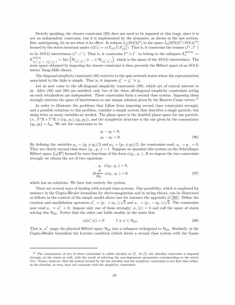
Figure 2: The face f and the two tetrahedra t and t′ are on the boundary of the triangulation,represented by the heavy dashed line. The link of the face is divided by the boundary into two parts.

3.6 Boundary terms

In ordinary Regge calculus boundary terms must be added to the action so that the equations of motionare the same when we vary the action with some boundary variables fixed. The other condition forboundary terms is that they add correctly. Consider a region of spacetime which is the union oftwo disjoint regions separated by a boundary, S = S′ ∪ S′′. The additivity condition is then thatS[S] = S[S′] + S[S′′] [35].

Consider for simplicity the part of the action (59) referring to a single face Sf = Tr[Bf (t)Uf (t)].Furthermore, choose two tetrahedra t and t′ appearing in the link around this face and break the linkin two so that the two tetrahedra belong now to the boundary (cf. Figure 2). The action can be splitto first order in the algebra as

Sf =1

2Tr[Bf (t)U1

tt′Rf ] +1

2Tr[Bf (t′)U2

t′tR−1f ] (79)

where in the second term of the sum we have replaced Bf (t) by Bf (t′) which, because of (41),

introduces terms of the second order in the lattice spacing. U(1,2)tt′ are just the boundary connection

variables. Here Rf is a fixed SO(4) element inserted to make the terms SO(4) covariant. Thus, theboundary action can be written in general as

S∂∆ =1

2

∑

f⊂∂∆

Tr[Bf (t)Utt′Rf ] (80)

with Utt′ given byUtt′ = Utt1(v1) ... Utnt′(vn). (81)

This gives additivity to first order in the algebra.

Let us remark on the specific case when the B’s are fixed on the boundary. In this case, in thecontinuum Plebanski theory, the boundary term is just

∫

B ∧A where A is the connection [36]. If wechoose Rf ≡ 1, the above discrete boundary action becomes

S∂∆ =1

2

∑

f⊂∂∆

Tr[Bf (t)Utt′ ] (82)

which reduces precisely to the continuum boundary action. Thus we choose Rf ≡ 1 when fixingthe B’s on the boundary. The boundary action is not gauge-invariant, as it is not in the continuum

15

theory.9

Let us now write the action for a single four simplex as it will be useful to us in the next section.All the faces are on boundary and so the action is just a sum of boundary terms. Explicitly:

Sv =1

2

∑

f⊂v

Tr[Bf(tA) UtAtB(v)] + Tr[λf UtAtB

(v) VtBv VvtA] (83)

3.7 Boundary variables

Suppose the triangulation ∆ has a boundary ∂∆. This boundary is a 3d manifold, triangulated bytetrahedra separated by triangles. Notice that, unlike what happens in the bulk, each boundarytetrahedron bounds just a single simplex of the triangulation; and each boundary triangle bounds justtwo boundary tetrahedra.

Let us identify the boundary variables, which reduce to the boundary gravitational field in thecontinuum limit. One boundary variable is simply Σf (t), where f is a boundary triangle and t isa boundary tetrahedron. There are only two boundary tetrahedra around f , one, t, at the start ofthe link as determined by the orientation of f , and the other, t′, at the end. It will turn out to beconvenient to use the notation ΣR

f and ΣLf for Σf (t) and Σf (t′). If desired, one can also associate

variables with the reverse orientation of f : ΣRf−1 := ΣL

f , ΣLf−1 := ΣR

f .

The other boundary variable is the group element Uf = Utt′ giving the parallel transport acrosseach triangle f bounding t and t′ (not to be confused with the holonomy (57) defined above). Noticethat (41) implies

UfΣRf U

−1f = ΣL

f . (84)

Finally, of the constraints (46, 47, 48, 43, 31), only (46, 47, 48, 43) act separately at each tetrahe-dron, and thus impose direct restrictions on boundary data. We call (46, 47, 48, 43) the kinematicalconstraints. The constraint (31) on the other hand necessarily involves bulk variables; we thus call itthe dynamical constraint.

The complex dual to the boundary triangulation defines a 4-valent graph Γ with nodes t (dual tothe boundary tetrahedron t) and links f (dual to the boundary triangle f). It is convenient to viewthe boundary variables as associated to the four valent graph Γ dual to the boundary triangulation:we have SO(4) group elements associated to the links of the graph and two Σ variables associatedto the two orientations of each such link. Accordingly, we change notation, and call l (for links) theoriented boundary triangles and n (for nodes) the boundary tetrahedra.

Since we are in a first order formalism, the space of these variables (ΣLl ,Σ

Rl , Ul) code the phase

space of discretized GR. In fact, this space is precisely the same as the phase space of a Yang-MillsSO(4) lattice theory, and it can be identified as the cotangent bundle of the configuration spaceC = SO(4)L, where L is the number of links on Γ.

This cotangent bundle has a natural symplectic structure, which defines Poisson brackets.

Ul, Ul′ = 0

(ΣLl )IJ , Ul′ = δll′ Ul τ

IJ

(ΣRl )IJ , Ul′ = δll′ τ

IJ Ul

(ΣRl )IJ , (ΣR

l )KL = δll′ λIJ KL

MN (ΣRl )MN (85)

9 One can also fix the U ’s on the boundary. In this case, there is no boundary term in the continuum theory. Thiscan effectively be achieved in the discrete theory by setting Rf = U−1

tt′after varying the action to obtain the equations

of motion (see appendix C).

16

where τIJ and λIJ KLMN are, respectively, the generators and the structure constants of SO(4). Observe

that the two quantities ΣRl and ΣL

l act very nicely as the right, and respectively, left invariant vectorfields on the group. Equation (84) gives the correct transformation law between the two.

However, it is important to notice a crucial detail at this point. As pointed out in [29] and in [26],because of its peculiar SU(2)× SU(2) structure, the cotangent bundle over SO(4) carries indeed two

different natural symplectic structures, related to one another by what Baez and Barrett call a flip:one is obtained from the other by flipping the sign of the antiselfdual part. That is, replacing Σ by B

Ul, Ul′ = 0

(BLl )IJ , Ul′ = δll′ Ul τ

IJ

(BRl )IJ , Ul′ = δll′ τ

IJ Ul

(BRl )IJ , (BR

l )KL = δll′ λIJ KL

MN (BRl )MN (86)

Both structures are equivalent to the lattice Yang Mills theory Poisson brackets [32], the difference isonly whether we identify the electric field with B or with Σ. We call (85) the “flipped” Poisson struc-ture (at the risk of some confusion, since Baez and Barrett call (86) the “flipped” Poisson structure.Being flipped as everything else, is a relative notion...)

Which one is the correct Poisson structure to utilize? The classical equations of motion, whichis the part of the theory that is empirically supported, do not determine the symplectic structureuniquely. In the Appendix C we study the direct construction of the symplectic structure from theaction. If we take the action (59) without the topological term (78), then we have the unflippedPoisson structure (86). (This is why we call it “unflipped”.) But in order to arrive at the Ashtekarformalism and LQG, we know that the topological term is needed. As shown in the appendix, thetwo symplectic structures written above are recovered by taking γ ≫ 1 and γ ≪ 1, respectively. Wediscard the first choice that gives macroscopic discrete area eigenvalue and we choose the second.10

Thus, we choose the flipped symplectic structure (85) as a basis for the quantization of theory. Thischoice leads to a nontrivial intertwiner space, while the opposite choice leads to the Barrett-Cranetrivial intertwiner space, as we shall see below.

3.8 Summary of the classical theory

Summarizing, discretized GR can be defined by the action (59) with the appropriate boundary terms(80) now defined as a function of the variables [Σf (t), Vvt, Utt′(v), λvf ]). That is

Sbulk[Σ, U, V, λ] =1

2

∑

f

Tr[Bf (t)Uf (t)] +∑

v

∑

f⊂v

Tr[λvfUtt′(v) Vt′v Vvt]. (87)

Plus the diagonal and off-diagonal simplicity constraints

Cff :=1

4∗Σf (t) · Σf (t) = 0, (88)

Cff ′ :=1

4∗Σf (t) · Σf ′(t) = 0.. (89)

The second can be replaced by the (stronger) condition that there is an nI for each t such that

nI ΣIJf (t) = 0, (90)

10Intermediate choices may also be of interest, but they lead to a more complicated quantum theory, involving alsonon-simple representations. See Appendix C.

17

equivalently, there is a gauge in whichΣ0i

f (t) = 0. (91)

The following two other constraints follow from the equations of motion

∑

f∈t Σf (t) = 0, (92)

andUtAtB

(v) = VtAv VvtB. (93)

4 Quantization

The quantization of the theory will proceed in three steps. First, we write the Hilbert space and theoperators that quantize the boundary variables and their Poisson algebra. Second, we impose thekinematical constraints (92,88,89,91). The first two of these pose no problem. The third one, namelythe nondiagonal simplicity constraints (89) require a careful discussion and some technical steps. Aswe shall see, we cannot impose these constraints strongly; we impose them weakly, in a sense definedbelow. Finally, the dynamics is specified by computing an amplitude for a state in the boundaryHilbert space [37, 38]. This amplitude is constructed by building blocks, the elementary buildingblock being a single four-simplex.

Remarkably, we will find that the physical Hilbert space that solves the constraints is naturallyisomorphic to the kinematical Hilbert space of SO(3) LQG. More precisely, it is isomorphic to the setof states of SO(3) LQG defined on the graph formed by the dual of the boundary triangulation. Ourkey result will then be a transition amplitude for a state in the Hilbert space of SO(3) spin networksdefined on the graph corresponding to the (dual of the) boundary of a four-simplex.

4.1 Kinematical Hilbert space and operators

The boundary phase space is the same as the one of an SO(4) lattice Yang-Mills theory. We quantizeit in the same manner as SO(4) lattice Yang-Mills theory [32]. That is, the natural quantization of thesymplectic structure of the boundary variables is defined on the Hilbert space HSO(4) := L2[SO(4)L],

formed by wave functions ψ(Ul) = ψ(g+l , g

−l ). The Ul variables are quantized as diagonal operators.

The variables ΣLl and ΣR

l are quantized as the left invariant —respectively right invariant— vectorfields on the group. These define a representation of the flipped classical Poisson algebra (85).

A basis in this space is given by the states

ψj+

lj−l

I+n I−

n(g+

l , g−l ) = 〈g+

l g−l |j+l , j−l , I+

n , I−n 〉 =

(

⊗

l

D(j+

l)(g+

l ) ·⊗

n

I+n

) (

⊗

l

D(j−l

)(g−l ) ·⊗

n

I−n

)

.

(94)Here D(j)(g) the are matrices of the SU(2) representation j: two of these are associated to each link;together, they form the SO(4) representation matrix (j+, j−), defined on the Hilbert space H(j+,j−).At each node, I+

n ∈ Hj+

1

⊗ · · · ⊗ Hj+

4

and I−n ∈ Hj−

1

⊗ · · · ⊗ Hj−

4

, so that I+n ⊗ I−n defines an element

of the space

H(j+

1,j

−

1)...(j+

4,j

−

4) :=

(

H(j+

1,j

−

1) ⊗ ...⊗H(j+

4,j

−

4)

)

(95)

associated to each node n with fixed adjacent representations (j+1 , j−1 )...(j+4 , j

−4 ). The contraction

pattern of the indices between the representation matrices and the tensors (I+, I−) is defined by Γ.

Next, we consider the constraints.

18

Strictly speaking, the closure constraint (92) does not need to be imposed at this stage, since it isnot an independent constraint, but it is implemented by the dynamics, as shown in the last section.But, anticipating, let us see what is its effect. It reduces L2[SO(4)L] to the space L2[SO(4)L/SO(4)N ]formed by the states invariant under ψ(Ul) = ψ(Vs(l)UlV

−1t(l) ). That is, it constrains the tensors (I+, I−)

to be SO(4) intertwiners (i+, i−). That is, it constrains I+ ⊗ I− to belong to the subspace KSO(4)t :=

KSO(4)

(j+

1,j

−

1)...(j+

4,j

−

4):= Inv

(

H(j+

1,j

−

1) ⊗ ...⊗H(j+

4,j

−

4)

)

, which is the space of the SO(4) intertwiners. The

state space obtained by imposing the closure constraint is then precisely the Hilbert space of an SO(4)lattice Yang-Mills theory.

The diagonal simplicity constraint (88) restricts to the spin network states where the representationassociated to the links is simple. That is, it imposes j+l = j−l ≡ jl.

Let us now come to the off-diagonal simplicity constraints (89), which are of central interest tous. After (92) and (88) are satisfied, only two of the three off-diagonal simplicity constraints actingon each tetrahedron are independent. These constraints form a second class system. Imposing themstrongly restricts the space of intertwiners to one unique solution given by the Barrett-Crane vertex.11

In order to illustrate the problems that follow from imposing second class constraints strongly,and a possible solutions to this problem, consider a simple system that describes a single particle, butusing twice as many variables as needed. The phase space is the doubled phase space for one particle,i.e., T ∗

R×T ∗R ∋ ((q1, p1), (q2, p2)), and the symplectic structure is the one given by the commutator

qa, pb = δab. We set the constraints to be

q1 − q2 = 0,

p1 − p2 = 0. (96)

By defining the variables q± = (q1 ± q2)/2 and p± = (p1 ± p2)/2, the constraints read: q− = p− = 0.They are clearly second class since q−, p− = 1. Suppose we quantize this system on the SchrodingerHilbert space L2[R

2] formed by wave functions of the form ψ(q+, q−). If we impose the two constraintsstrongly we obtain the set of two equations

q− ψ(q+, q−) = 0,

i~∂

∂q−ψ(q+, q−) = 0. (97)

which has no solutions. We have lost entirely the system.

There are several ways of dealing with second class systems. One possibility, which is employed forinstance in the Gupta-Bleuler formalism for electromagnetism and in string theory, can be illustratedas follows in the context of the simple model above (see for instance the appendix of [39]). Define the

creation and annihilation operators a†− = (p− + iq−)/√

2 and a− = (p− − iq−)/√

2. The constraints

now read a− = a†− = 0. Impose only one of these strongly: a−|ψ〉 = 0 and call the space of statessolving this Hph. Notice that the other one holds weakly, in the sense that

〈φ|a†−|ψ〉 = 0 ∀ φ, ψ ∈ Hph. (98)

That is, a†− maps the physical Hilbert space Hph into a subspace orthogonal to Hph. Similarly, in theGupta-Bleuler formalism the Lorentz condition (which forms a second class system with the Gauss

11 The commutator of two of these constraints is called chirality in [7]. In [7], the chirality constraint is imposedstrongly on the states as well, with the result of selecting the non-degenerate geometries corresponding to the sector(51). Notice, however, that the system formed by the the chirality and the simplicity constraints is not first class either,as the chirality, in turn, does not commute with the simplicity constraints.

19

constraint) holds in the form

〈φ|∂µAµ|ψ〉 = 0 ∀ φ, ψ ∈ Hph. (99)

A general strategy to deal with second class constraints is therefore to search for a decompositionof the Hilbert space of the theory Hkin = Hphys ⊕ Hsp (sp. for spurious) such that the constraintsmap Hphys → Hsp. We then say that the constraints vanish weakly on Hphys. This is the strategywe employ below for the off-diagonal simplicity constraints Cll′ . Since the decomposition may not beunique, we will have to select the one which is best physically motivated. We now define this space.

4.2 The physical intertwiner state space Kph

Consider the state space obtained by imposing the diagonal simplicity constraint, namely by takingj+l = j−l := jl, but not the closure constraint yet. Let us restrict attention to a single tetrahedront. The constraints (89) at t act on the space associated to t, which is H(j1,j1)...(j4,j4). The closure

constraint will then restrict this space to the SO(4) intertwiner space KSO(4)t . We search for a subspace

Kph of KSO(4)t where the nondiagonal constraints vanish weakly.

First, note KSO(4)t = Inv(H(j1,j1) ⊗ ...H(j4,j4)) is a subspace of the larger space

H(j1,j1) ⊗ ...H(j4,j4) = Hj1⊗j1 ⊗ ...Hj4⊗j4 (100)

which can be thought of as a tensor product of carrying spaces of SO(4) representations or SU(2)representations, as desired. The Clebsch-Gordan decomposition for the first factor on the right-handside above gives

Hj1⊗j1 = Hj1 ⊗Hj1 = H0 ⊕H1 ⊕ · · · ⊕ H2j1 (101)

and similarly for the other factors. By selecting the highest spin term in each factor, we obtain asubspace

H2j1 ⊗ · · · ⊗ H2j4 . (102)

Orthogonal projection of this subspace into KSO(4)t then gives us the desired Kph ⊂ KSO(4)

t . This Kph

is the intertwiner space that we want to consider as a solution of the constraints. The total physicalboundary space Hph of the theory is then obtained as the span of spin-networks in L2[SO(4)L/SO(4)N ]with simple representations on edges and with intertwiners in the spaces Kph at each node. Noticethat the elements in Kph are not necessarily simple in their internal representation, in any basis. Letus study the properties of the space Kph, and the reasons of its interest.

(i) First, it is easy to see that the off-diagonal simplicity constraints (89) vanish weakly Kph, in the

sense stated above. This follows from the following consideration. A generic element of KSO(4)t

can be expanded as

|ψ〉 =∑

i+i−

ci+i− |i+, i−〉 (103)

where i± defines a basis in the SU(2) intertwiner space. The off-diagonal simplicity constraintsare odd under the exchange of i+ and i−, namely under exchange of self dual and antiselfdualsectors. But the states in Kph are symmetric in i+ and i−. Hence 〈φ|Cll′ |ψ〉 = 0, ∀φ, ψ ∈ Kph,that is, Kph can be considered as one possible solution of the constraint equations.

(ii) Second, let us motivate the choice of this solution. Recall that the off-diagonal simplicity con-straints can be expressed as the requirement that there is a direction nI such that (91) holds.But this is precisely the “classical” limit of the condition satisfied by the spin-2j representation,

20

as observed at the end of Section 2.2. That is, promoting (91) to the quantum theory gives therequirement that there there is a gauge in which

J0i = 0. (104)

which is (27), namely the condition satisfied by the spin-2j component of the representation(j, j). Equivalently, (91) implies

2C4 =1

2JIJ

l Jl IJ =1

2J ij

l Jl ij = C3 (105)

where C4 is the SO(4) scalar Casimir in the representation Hjl,jland C3 is the Casimir of the

SO(3) subgroup that leaves nI invariant, in the same representation. As it is, this relationhas in general no solution in Hjl,jl

, but if we order it in slightly different manner, as in (24),(reinstating ~ 6= 0 for clarity)

C =√

C3 + ~2/4 −√

2C4 + ~2 + ~/2 = 0 (106)

then there is always a solution, which is given by the H2j subspace of Hj,j . Therefore the off-diagonal simplicity constraints pick up precisely the space we have defined. In other words, thisspace satisfies a quantum constraint, which in the classical limits becomes the classical constraint(105).

Notice that if we hadn’t chosen the flipped symplectic structure, then we would have obtainedJ ij = 0, instead of J0i = 0, that is, the vanishing of the SO(3) Casimir. Following the sameprocedure as above, we would have defined the space

K(0)ph = Inv (H0 ⊗ ...⊗H0) ⊂ Hj1...j4 (107)

and this is precisely the one dimensional Barrett-Crane intertwiner space. That it, it is thechoice of the flipped symplectic structure that allows the selection of a nontrivial intertwinerspace.

(iii) Third, we have the remarkable result that Kph is isomorphic to the SO(3) intertwiner space,and therefore the constrained boundary space Hph is precisely the SO(3) LQG state spaceHSO(3) associated to the graph which is dual to the boundary of the triangulation, namelythe space of the SO(3) spin networks on this graph. We exhibit this isomorphism in a waythat simultaneously shows a new way of viewing Hph. We will first construct a projectionπ : HSO(4) → HSO(3). The hermitian conjugate map will then be an embedding f : HSO(3) →HSO(4). The image of this embedding will be none other than Hph.

The map π : HSO(4) → HSO(3) is simple to construct. Choose an SO(3) subgroup H of SO(4).As explained in Section 2.2, this choice is equivalent to the choice of an isomorphism betweenthe two SU(2) factors of SO(4). A (simple) SO(4) representation H(j,j) is in general a reducible

representation of H : since H acts on each duality component independently, it transforms asH(j,j) = Hj ⊗ Hj , where Hj is the standard spin-j representation of SU(2). This decomposesinto irreducibles as

H(j,j) = H0 ⊕H1 ⊕ ...⊕H2j , (108)

Thus, begin with an SO(4) spin-network state Ψ, and consider the restriction Ψ| l×H

to the

subgroup H on each edge. As Ψ is SO(4) invariant, it is in particular H-invariant, and thus therestriction Ψ| l

×His a sum of SO(3) spin-networks. Furthermore, because Ψ is SO(4) invariant,

and because all possible SO(3) subgroups H are related to each other by conjugation, this sumof spin-networks is independent of the choice of SO(3) subgroup H . The above considerations

21

tell us that this sum is just that given by the above Clebsch-Gordan decomposition for each edge.The result of the projection πΨ is then defined to be the spin-network in this sum correspondingto the highest weight spin on each edge. Thus π so-defined maps simple SO(4) spin-networkstates to SO(3) spin-network states. The spin (j, j) on each edge of the SO(4) spin-network ismapped to spin 2j in the SO(3) spin-network. Each SO(4) intertwiner Iv ∈ InvSO(4)(H(j1,j1) ⊗... ⊗ H(j4,j4)) is mapped to an SO(3) intertwiner simply via orthogonal projection onto thesubspace InvSU(2)(H(2j1) ⊗ ...⊗H(2j4)) ⊂ (H(2j1) ⊗ ...⊗H(2j4)).

Let us now describe the conjugate embedding f : HSO(3) → Hph. This is defined as the hermitianconjugate of π, using the fact that π is a linear map between Hilbert spaces. Let us describe itin detail.

Let us first describe the embedding f restricted to a single intertwiner space, namely the map(that we also call) f from the space KSO(3) of the SO(3) intertwiners to Kph. Consider anintertwiner i ∈ KSO(3), between the four representations (2j1...2j4). Contract it with fourtrivalent intertwiners between the representations (2ja, ja, ja), the edge with spin 2j1 beingcontracted with the 2j1 edge of the corresponding trivalent intertwiner, etc. This gives us atensor e(i) in (H(j1,j1) ⊗ ... ⊗ H(j4,j4)). e(i) is not an SO(4) intertwiner, because it is notSO(4) invariant, but we obtain an SO(4) intertwiner by projecting it in the invariant part of(H(j1,j1) ⊗ ...⊗H(j4,j4)). Since SO(4) is compact, this projection can be implemented by actingwith a group element U in each representation, and integrating over SO(4).

f(i) :=

∫

SO(4)

dV

(

⊗

l

D(λl)(V )

)

· e(i) (109)

The SO(4) action can be factorized into two SU(2) group elements, one acting on the self dual,and other on the anti-selfdual representations. One of the two factors can be eliminated byvirtue of the SU(2) invariance of the trivalent intertwiners and i. What remains is an SU(2)integration over just one of the representations. Using the well known relation

∫

SU(2)

dgDa1b1(g)...Da4b4(g) =∑

i

ia1...a4ib1...b4 (110)

it is easy to see that we have

f |i〉 =∑

i+i−

f ii+i− |i+i−〉 (111)

where the coefficients f ii+i−

are given by the evaluation of the spin network

i i i

j

jj j

j

j

jjj j

+ −

1

1

jj

2

3

2

3

44

1

2

3

4

2

2

2

2

.

If we piece these maps at each node, we obtain the map f : HSO(3) → Hph of the entire LQGspace into the state space of the present theory. In the spin network basis we obtain

f : |jl, in〉 7−→∑

i+n ,i

−

n

f in

i+n ,i

−

n

|jl/2, jl/2, i+n , i−n 〉. (112)

22

Equivalently, writing explicitly the states as functions on the groups,

f :

(

⊗

l

D(jl)(gl)

)

·(

⊗

n

in

)

7−→

∫

SO(4)N

∏

n

dVn

(

⊗

l

D(jl2

,jl2

)(

Vs(l)(g+l , g

−l )V −1

t(l)

)

)

·(

⊗

n

e(i)n

)

(113)

where indices have been omitted and s(l), t(l) stand resp. for source and target of the link l.This completes the definition of the projection and the corresponding embedding of the Hilbertspace of LQG into the boundary Hilbert space of the model.

(iv) Let us illustrate more in detail the construction in (iii) using the standard spinor notation[40]. The vectors in Hj can be represented as totally symmetric tensors with 2j spinor indices(A1...A2j) ≡ A, where each index A = 0, 1 is in the fundamental representation of SU(2). Anelement in H(j1,j1)...(j4,j4) has therefore the form

I(A1...A2j1)(A′

1...A′

2j1)...(D1...D2j4

)(D′

1...D′

2j4) =: IAA′...DD′

(114)

here primed and unprimed indices are symmetrized independently; they live in the self dual andantiself dual components of the representation. Round brackets stand for symmetrization. Bychoosing to no longer distinguish between primed and unprimed indices, this SO(4) intertwinerI between the simple representations (j1, j1)...(j4, j4) becomes a tensor among the SU(2) rep-resentations j1 ⊗ j1, j2 ⊗ j2, j3 ⊗ j3, j4 ⊗ j4. Because of the SO(4)-invariance of I, the resultingSU(2) tensor does not depend on the way primed and unprimed indices are identified.

Let us first construct the projection π, and corresponding embedding f , for individual intertwinerspaces. The projection π : KSO(4) → KSO(3) is simply given by symmetrizing over the spinorindices associated with each link

π : IAA′...DD′ 7−→ I(AA′)...(DD′) =: ia...d (115)

where the index a is short for (AA′) := A1 . . . A2j1A′1 . . . A

′2j1

, and similarly for b,c, and d. Thissymmetrization projects I to an SU(2) intertwiner among the representations 2j1, 2j2, 2j3, 2j4,thereby selecting the highest weight irreducible representation in the decomposition j ⊗ j =0⊕· · ·⊕2j on each edge. Notice that 2j ∈ Z so that the projected intertwiner transforms underSO(3) transformations.

Next, we write, for j1, . . . j4 ∈ Z, the corresponding embedding f : KSO(3) → KSO(4). First,the embedding e is trivially obtained by reading the indices AA′ as living in self-dual andanti-self-dual representations, respectively:

e : ia...d 7−→ e(i)AA′...DD′

:= iAA′...DD′

(116)

This is not yet a SO(4) intertwiner and in order to recover an element of the invariant subspacewe have to “group average” as in equation (109).

Let us now consider the projection, and corresponding embedding, for individual spins. Considerthe state space for a single link – that is, the space of square integrable functions over one single

copy of SO(4). This space is spanned by the representation matrices D(j+,j−) (Ul)AA′

BB′ whereUl = (g+

l , g−l ) ∈ SO(4) and g±l ∈ SU(2). Here we restrict ourselves to simple representations

(j, j). For such representation matrices, the projection is defined by

π : D(j,j)(g+l , g

−l )AA′

BB′ 7−→ D(j,j)(gl, gl)(AA′)

(BB′) = D(2j)(gl)a

b. (117)

23

That is, we first restrict to a diagonal subgroup (g, g) ⊂ SO(4); such a subgroup is isomorphicto SO(3). The (j, j) SO(4)-representation matrix then becomes a j ⊗ j SU(2)-representationmatrix; from there we project to the highest SU(2) irreducible, namely the 2j representation,as before. The corresponding embedding of SO(3) spins into SO(4) spins is then obviously2j 7→ (j, j).

Putting together the embeddings for intertwiners and spins, we obtain the embedding (113) ofSO(3) LQG states into the SO(4) boundary state space of the model.

(v) Lastly, with the embedding proposed in (iii,iv) above, and in light of (53), the constraints (105)being used to solve the off-diagonal simplicity constraints simply express the condition thatthree-dimensional areas as determined by the SO(4) theory match three-dimensional areas asdetermined by LQG.

This concludes the discussion on the implementation of the constraints. The last point to discuss isthe dynamics.

4.3 Dynamics

Following the strategy stated at the start of this section, consider a triangulation formed by a single4-simplex v. Denote the boundary graph by Γ5. A generic boundary state (satisfying all kinematicalconstraints) is a function Ψ(Uab), where a, b = 1, ..., 5, in the image f [HLQG]. We begin by writing thetransition amplitude between sharp values of the B’s. From this we deduce the amplitude in terms ofthe U’s, and then compute the amplitude for the quantum state Ψ(Uab). Beginning this procedure,

A(Bab) =

∫

∏

a

dVa

∏

(ab)

eiTr[BabV −1a Vb]

=

∫

∏

a

dVa

∏

(ab)

dUab eiTr[BabUab] δ(VaUabV

−1b )

=

∫

∏

(ab)

dUab eiTr[BabUab]

∫

∏

a

dVa δ(VaUabV−1b ) (118)

so that the amplitude in the connection representation reads:

A(Uab) =

∫

∏

a

dVa δ(VaUabV−1b ). (119)

The integral is over a choice of SO(4) element V at each node. Let us define the bra

〈W | =

∫

∏

(ab)

dUab A(Uab)〈Uab|. (120)

The quantum amplitude for a given state |ψ〉 in the boundary Hilbert space is:

A(Ψ) := 〈W |Ψ〉 (121)

As Ψ satisfies all the kinematical constraints, it is of the form Ψ = f(ψ) for some ψ ∈ HLQG. Let usconsider the specific case when ψ is a spin-network state ψ = ψjab,ia. The amplitude is then givenexplicitly by

A(jab, ia) := A(ψjab,ia) =∑

ia+

ia−

15j

((

jab

2,jab

2

)

; (ia+, ia−)

)

f ia

ia+

ia−

(122)

24

as can be easily seen by using (112) and decomposing (119) in the SO(4) spin-network basis. Thisamplitude extends by linearity to more general states Ψ = f(ψ).

When we have a number of transitions between different 4-simplices, we have to sum over boundarystates around each, projecting each onto this state 〈W |. This gives transition amplitudes for boundarySO(3) spin networks with the amplitude generated by the partition function

Z =∑

jf ,ie

∏

f

(dim jf2)2∏

v

A(jf , ie). (123)

Observe that the quantum dynamics defined above does not change if we add the topologicalterm (78) incorporating γ. For, by changing the integration variable to Πf := Bf + 1

γ⋆ Bf in the

path-integral, the above derivation goes through in exactly the same manner, and the final vertexamplitude differs at most by a constant, as determined by the Jacobian of the transformation from Bto Π (see appendix C).

The problem is whether this quantum dynamics defines a non-trivial theory with general relativityas its low energy limit. A way of systematically exploring the low-energy behavior of a backgroundindependent quantum theory has recently been developed (after a long search; see for instance [41])in [15]. These techniques should shed some light on this problem.

5 Conclusions

We close with three observations.

(i) There is a relation of the SO(4) states determined in this model to the projected spin networkstates studied by Livine in [42]. (A similar approach is developed by Alexandrov in [44].) Theconstrained SO(4) states that form the physical Hilbert space of the model presented here can beconstructed from (the euclidean analog of) these projected spin networks. The Euclidean analog ofthe projected spin networks defined in [42] are wavefunctions Ψ[Ul, χn] depending on an SO(4) groupelement for each link, and a vector χn ∈ SO(4)/SO(3) at each node. The wavefunctions are labelledby an SO(4) representation (j+l , j

−l ) for each link, an SU(2) representation jnl for each node and link

based at that node, and an SU(2) intertwiner at each node. The SO(4) spin-networks of the presentpaper can be obtained from these projected spin networks by (i) setting j+l = j−l ≡ jl, (ii) settingjnl = j+l + j−l = 2jl, and (iii) averaging over χn at each node (concretely this averaging can be doneby acting on each χn with an SO(4) element Un, and then averaging over the Un’s independentlyusing the Haar measure). Each of these three steps corresponds directly to solving (i) the diagonalsimplicity constraints, (ii) the off-diagonal simplicity constraints, and (iii) the Gauss constraint.

(ii) Livine and Speziale have found an independent derivation of the vertex proposed here [45],based on the use of the coherent states they have introduced in [18].

(iii) The discreteness introduced by the Regge triangulation should not be confused with thequantum-mechanical discreteness. The last is realized by the fact that variables that give a physicalsize to a Regge cell turn out to have discrete spectrum. However, the two “discretenesses” end up tobe related, because, due to the quantum discreteness, in the quantum theory the continuum limit ofthe Regge triangulation turns out to be substantially different that the continuum limit of, say, latticeQCD or classical Regge calculus. Intuitively, one can say that no further triangulation refinementcan capture degrees of freedom below the Planck scale, since these do not exist in the theory. Theultraviolet continuum limit is trivial in the quantum theory (for a discussion of this point, see [3]).Thus, in the quantum theory the Regge triangulation receives, so to say a posteriori, the physicalinterpretation of a description of the fundamental discreteness of spacetime (the one, say, that makesgravitational entropy finite [46]). Numerous approaches to quantum gravity start from the assumptionof a fundamental spacetime discreteness ([47]); others use spacetime discreteness as a regularization

25

to be removed ([48]); the conventional formulation of loop quantum gravity derives the discretizationof spacetime from the quantization of continuum general relativity. The derivation of loop quantumgravity given here is somewhat intermediate: it starts from a lattice discretization, and later finds outthat in the quantum theory, say, the area of the triangles of the triangulation is discrete and thereforethe regularization receives a physical meaning. See also [27].

In summary. We have considered the Regge discretization of general relativity. We have describedit in terms of the Plebanski formulation of GR. We have quantized the theory, on the basis of aflipped Poisson structure and imposing the off-diagonal simplicity constraints weakly. This new wayof imposing the simplicity constraints is weaker. This weakening of the constraints is motivated bythe observation that they do not form a closed algebra, as well as by the realization that a richerboundary space is needed for a correct classical limit [14].

The theory we have obtained is characterized by the fact that its boundary state space exactlymatches that of (SO(3)) loop quantum gravity. This can be seen as an independent derivation ofthe loop quantum gravity kinematics, and, in particular, of the fact that geometry is quantized. Avertex amplitude has then been derived from the discrete action, leading to a spin-foam model givingtransition amplitudes for loop quantum gravity states.

We expect that the model considered here will admit a group field theory formulation [30] andthat its vertex can be used to generate the dynamics of loop quantum gravity also in the absence ofa fixed triangulation [3]. Whether this model is non-trivial and/or reproduces general relativity in anappropriate limit we do not know. Study of its semi-classical limit and n-point functions [15] shouldshed light on the discussion.

————————————

Thanks to Alejandro Perez for help, criticisms and comments, to Sergei Alexandrov, Etera Livine,Daniele Oriti and Simone Speziale for useful discussions. JE gratefully acknowledges support by anNSF International Research Fellowship under grant OISE-0601844

A 4-simplex geometry as gravitational field

In the way we have defined the Regge triangulation above, the degrees of freedom of the gravitationalfield are captured by the geometry of each 4-simplex. Consider in each 4-simplex v Cartesian coordi-nates such that one vertex of the 4-simplex, say the vertex 5, has coordinates (v5)

a = 0, and the otherfour vertices have coordinates (vb)

a = δab . In these coordinates, the metric will not necessarily be δab,

but rather take a form gab(v). The full information about the geometry of the four simplex v is thencoded into the ten quantities gab(v). Notice indeed that the shape of a 4-simplex in R4 is determinedby 10 quantities (for instance the length of its ten sides), and therefore the ten components of gab(v)are the correct number for capturing its degrees of freedom (possibly up to discrete degeneracies).

In particular, gaa (we will often drop the argument (v) in the rest of this appendix, since wedeal here with a single 4-simplex) are (the square of) the lengths of the four edges adjacent to the5th vertex, and gab are essentially the angles between these edges. (Also: gaa is the volume of thetetrahedron a, opposite to the vertex a, and gab is the variable giving the angle between the normalsto the tetrahedra a and b.)

Thus, the discretized variables can be taken to be the ten quantities gab(v). This is of course nosurprise at all, since this is precisely a direct discretization of the variable gab(x) used by Einstein todescribe the gravitational field, here reinterpreted simply as a way to represent the geometry of eachelementary 4-simplex.

Another way of determining the geometry of a four simplex is to give its ten areas. Let A =1, 2, 3, 4, 5 label the five tetrahedra bounding the 4-simplex. The tetrahedron 1 is the one with vertices2,3,4,5, and so on cyclically. Let fAB denote the triangle bounding the two tetrahedra A and B. The

26

triangle f12 has vertices 3, 4, 5, and so on cyclically. Let AAB ≡ AfABbe the area of the triangle fAB.

Consider in particular the six areas Aab ≡ Afab, of the six faces adjacent to the vertex 5. A short

computation, for instance using (53), shows that

A2ab = gaagbb − gab. (124)

Define the angle variables Jaabc ≡ Jfabfac, related to the angle between the triangles fab and fac. (We

can also write A2ab = Jaabb.) Then again:

Jaabc = gaagbc − gabgac. (125)

The closure relation of the bivectors of a tetrahedron implies

A215 = A2

12 +A213 +A2

14 + 2(J1123 + J1134 + J1142) (126)

and so on cyclically. The six equations (124) and the the four equations (126) express the ten areas asfunctions of the ten components of the metric. Inverting these equations gives the metric as a functionof the areas: gab(AAB), and then, via (125), the angles as functions of the areas: JAABC(AAB).Therefore the full geometry of one 4-simplex is determined by the ten areas AAB . Computing the twofunctions gab(AAB), and JAABC(AAB) explicitly would be of great utility for quantum gravity.

B Existence of tetrad

In this appendix we show that the constraints (46, 47, 48), at the classical discretized level, aresufficient to imply the existence of a tetrad eI

µ associated with each tetrahedron t. The main point is

that the ‘dynamical constraint’ (49 or 50) is not needed for the existence of eIµ(t). Rather, as explained

in the main text, the role of (49) or (50), or its reformulation as (31), is to ensure that the geometriesof the tetrahedra in a single 4-simplex fit together to form a single 4-geometry.

The triad portion of the tetrad eIµ(t) associated with the 3-plane of the tetrahedron t is uniquely

determined (up to an overall sign) by the B(t)’s of the faces of the tetrahedron. The last componentof the tetrad associated with the normal to t, however, is not determined by the B(t)’s associatedwith t. This final component is fixed only upon comparing with the tetrads at the other tetrahedrain the 4-simplex via the parallel transport maps Utt′(v).

Let us make all of this precise. Let Σ denote the portion of space-time associated with one of the4-simplices v. Σ is a 4-manifold. Equip the tangent bundle of Σ with a background flat connection(so that we have a natural notion of parallel translation between any two points, and a natural notionof straightness).12 In v, consider a tetrahedron t with faces labeled 1,2,3, and 4. For each face, we letBµν

i denote the associated bivector living in the tangent space of Σ. These bivectors satisfy

4∑

i=1

Bµνi = 0. (127)

What we wish to show in this appendix is that the discretized constraints (46, 47, 48) are sufficientto imply that either

BIJi = Bµν

i eIµe

Jν (128)

12 Within a single 4-simplex, or any non-closed chain of 4-simplices, the choice of such a connection is a pure gaugechoice.

27

or∗BIJ

i :=1

2ǫIJ

KLBKLi = Bµν

i eIµe

Jν (129)

for some tetrad eIµ(t). We begin with a

Lemma 1. If eIµ is such that BIJ

i = Bµνi eI

µeJν for i ∈ 1, 2, 3, and

4∑

i=1

BIJi = 0, (130)

then BIJ4 = Bµν

4 eIµe

Jν as well. An analogous statement holds with BIJ

i replaced by ∗BIJi .

Proof.

Using (130) and then (127),

BIJ4 = −

3∑

i=1

BIJi = −

3∑

i=1

Bµνi eI

µeJν = Bµν

4 eIµe

Jν . (131)

The proof for the ∗BIJi is similar. 2

.

Thus, if we find a tetrad compatible with only BIJ1 , BIJ

2 , BIJ3 (in the sense of (128) or (129)), then

by imposing equation (130) (the closure constraint), BIJ4 will then automatically be compatible with

the same tetrad, in the same sense. In other words, by using the closure constraint, we can ignoreBIJ

4 .

Let p denote the point in the tetrahedron shared in common by faces 1,2, and 3. Let vµ1 , v

µ2 , v

µ3

denote the three edges emanating from this point, numbered such that face 1 is between vµ2 and vµ

3 ,etc, cyclically. Then we can choose our sign conventions such that

Bµν1 = 2v

[µ2 v

ν]3 , and cyclically. (132)

Specifying a tetrad eIµ is then equivalent to specifying the three internal vectors

eIi := vµ

i eIµ, i ∈ 1, 2, 3, (133)

and the external unit normal nµ to the tetrahedron. In terms of the tetrad,

nµ := eIµnI (134)

where nI is the unit normal to spanvµ1 e

Iµ, v

µ2 e

Iµ, v

µ3 e

Iµ. In terms of these variables, the condition

BIJi = Bµν

i eIµe

Jν for i ∈ 1, 2, 3 becomes

BIJ1 = 2e

[I2 e

J]3 , and cyclically. (135)

and likewise the condition ∗BIJi = Bµν

i eIµe

Jν becomes

∗BIJ1 = 2e

[I2 e

J]3 , and cyclically. (136)

We are now in a position to state the principal proposition and sketch its proof.

Proposition 2. If BIJ1 , BIJ

2 , BIJ3 are linearly independent and are such that

∗Bi · Bj = 0, i, j ∈ 1, 2, 3 (137)

then exactly one of the two following cases hold.

28

1. There exists eI1, e

I2, e

I3 such that

BIJ1 = 2e

[I2 e

J]3 and cyclically, (138)

or

2. there exists eI1, e

I2, e

I3 such that

∗BIJ1 = 2e

[I2 e

J]3 and cyclically. (139)

In either case, (eI1, e

I2, e

I3) is unique up to (eI

1, eI2, e

I3) 7→ (−eI

1,−eI2,−eI

3).

Proof.

Equation (137), for the case i = j, using proposition (3.5.35) of [40], tells us that there existsαI

i , βIi , γ

Ii , δ

Ii such that

BIJi = 2α

[Ii β

J]i (140)

∗BIJi = 2γ

[Ii δ

J]i (141)

(i = 1, 2, 3). From the linear independence of the B’s, we know in particular that none of them arezero. Therefore, if we define for each i

Vi := spanαi, βi (142)

Ui := spanγi, δi, (143)

then Vi and Ui are each two dimensional. Vi is just the two dimensional subspace uniquely determinedby the bivector BIJ

i , whereas each Ui is just the subspace uniquely determined by the bivector ∗BIJi .

Let us now look at the rest of the equations (137). For each i 6= j, they tell us that αi, βi, αj , βjand γi, δi, γj , δj are each linearly dependent. Vi and Vj therefore non-trivially intersect, as do Ui

and Uj, so that

dim(Vi ∩ Vj) > 0 (144)

dim(Ui ∩ Uj) > 0. (145)

But the linear independence of the B’s tells us that none of the V ’s can be the same, and none of theU ’s can be the same. Thus, for i 6= j,

dim(Vi ∩ Vj) < 2 (146)

dim(Ui ∩ Uj) < 2, (147)

whence

dim(Vi ∩ Vj) = 1 (148)

dim(Ui ∩ Uj) = 1. (149)

Let f I1 be any non-zero vector in V2 ∩ V3, etc cyclically. Likewise let f I

1 be any non-zero vector inV2 ∩ V3, etc cyclically. One can prove that exactly one of spanf1, f2, f3 and spanf1, f2, f3 is threedimensional, and the other is one dimensional. To prove this is non-trivial; we leave it as an exerciseto the reader. In proving this, one uses in a key way both the assumption that the B’s are linearlyindependent and the fact that for each i, Vi and Ui are orthogonal complements (which one can alsoshow).

29

In the case where f1, f2, f3 is linearly independent, by setting ei = λifi, one can solve for λi

such that (138) holds. These λi are unique up to (λ1, λ2, λ3) 7→ (−λ1,−λ2,−λ3), so that ei is uniqueup to (e1, e2, e3) 7→ (−e1,−e2,−e3). Furthermore, one can show the fact dim(spanf1, f2, f3) = 1implies that there exists no ei such that (139) holds.

In the case where dim(spanf1, f2, f3) = 1 and f1, f2, f3 is linearly independent, the situationsare obviously reversed. There exist no ei such that (138) holds, whereas there exist ei’s unique up to(e1, e2, e3) 7→ (−e1,−e2,−e3), such that (139) holds.

Thus we have the proposition. 2

.

C Symplectic structure

The action is

S =1

2

∑

f∈int∆

Tr(Bf (t)Uf (t)) +1

2

∑

f∈∂∆

Tr(BfUfRf ). (150)

In the case when one fixes the B variables on the boundary, one sets Rf = identity, as then theboundary term reduces to the usual classical boundary term appropriate when fixing the B variableson the boundary [36]. When one fixes the U ’s (i.e., the connection) on the boundary, analogy withthe classical theory suggests that there should be no boundary term. However, in a discrete theorythis is not literally possible, as then no boundary variables would appear in the action at all. Forthe case of fixing the U ’s on the boundary, we therefore suggest the following prescription. We wantthe terms in the boundary sum to essentially be the same as the terms in the interior sum: thiswill be the case if Rf is the holonomy around the rest of the link of f outside of ∆. Of course, theproblem is that this part of the holonomy around f is not determined by any dynamical variables.We propose the following prescription. Whenever varying the action, keep the Rf ’s fixed; however,whenever evaluating anything on extrema of the action, set Rf equal to what we know it ‘should’be: namely, the holonomy along the part of the link of f outside of T as determined by the BFequations of motion. The BF equations of motion dictate that all holonomies around closed loopsare trivial. Thus, our prescription is, whenever evaluating an expression onshell, set Rf = U−1

f . Aremark is in order as to why the BF equations of motion are used. The BF equations of motion are theequations of motion coming from the unconstrained action (150). We use the unconstrained action inderiving the symplectic structure because our general philosophy is that we are quantizing GR as aBF theory constrained at the quantum level. That is, we first compute the symplectic structure andquantize everything as though it were pure BF theory. Only then, after the ‘kinematical’ quantizationis complete, do we impose the simplicity constraints and obtain GR.

Let us determine the symplectic structure from the action, when we fix the U ’s on the boundary.We will use a method essentially coming from that described in [49], and briefly mentioned in [2];the method is the following. We first apply an arbitrary variation δ to the action without fixing anyvariables on the boundary; then we restrict to solutions of the equations of motion. The result will bea boundary term Θ(δ) depending linearly on the variation. This gives us a linear map from variations(at the space of solutions) into real numbers. This linear map is then extended off-shell basicallyby keeping the same expression in terms of the basic variables.13 We thereby obtain a linear mapΘ from arbitrary variations of boundary data into real numbers — that is, a one-form on the space

13If there are constraints, this expression has ambiguities. One uses the “obvious”, simplest expression in this case.

30

of boundary data. This Θ is the canonical one form on the boundary phase space. The symplecticstructure is then the exterior derivative Ω = ddΘ.

Let us apply this procedure. Varying the action (150) gives

δS =1

2

∑

f∈int∆

Tr((δBf )Uf (t)) +1

2

∑

f∈int∆

Tr(Bf (t)(δUf (t)))

+1

2

∑

f∈∂∆

Tr((δBf )UfRf ) +1

2

∑

f∈∂∆

Tr(Bf (δUf )Rf ). (151)

Next, restrict to the case of B’s and U ’s that satisfy the equations of motion. Then, when δUf onthe boundary is zero for f ∈ ∂∆, the entire expression above must vanish. But only the fourth termdepends on δUf for f ∈ ∂∆. Therefore, the other terms must vanish (on solutions) no matter whatis δU on the boundary. Therefore, on solutions, at most the fourth term above can survive, and wehave

δS =1

2

∑

f∈∂∆

Tr(Bf (δUf )Rf ). (152)

Applying the equations of motion to Rf , we finally set Rf = U−1f , giving us

Θ(δ) =1

2

∑

f∈∂∆

Tr(Bf (δUf )U−1f ). (153)

Extending Θ to arbitrary variations of the boundary data, keeping the same expression in terms ofthe basic variables, we obtain the canonical one-form

Θ(δ) =1

2

∑

f∈∂∆

Tr(Bf (δUf )U−1f ). (154)

We next claim that[

(δUf )U−1f

]IJ is an element of so(4). To show this, let Uf (λ) denote a one-

parameter path in SO(4) such that δ is the tangent to the path at λ = 0. Then

(δUf )U−1f =

d

dsUf (s)|s=0Uf (0)−1 =

d

ds[Uf(s)Uf (0)−1]s=0 (155)

The argument in brackets is the identity at s = 0, so that one has the action of a tangent vector atthe identity on the matrix elements of the group. Thus one has an element of the Lie algebra.

Introduce a basis ξαα=1,...6 of so(4), orthonormal with respect to the trace — i.e. such thatTr(ξαξβ) = −ξIJ

α ξβIJ = −δαβ . Denote the components of a Lie algebra element with respect to thisbasis just by adding a α, β, γ . . . superscript or subscript. (154) can then be written

Θ(δ) = −1

2

∑

f∈∂∆

(Bf )α

[

(δUf )U−1f

]α. (156)

Defineµf (δ)α :=

[

(δUf )U−1f

]α(157)

so that µαf is a one-form on the copy of SO(4) parametrized by Uf . We can then write the canonical

one form Θ as

Θ = −1

2

∑

f∈∂∆

(Bf )αµαf . (158)

31

For each face f , and each basis element ξα ∈ so(4), let δRf,α denote the corresponding right invariant

vector field on the associated copy of SO(4). We then have

µf (δRf,α)β = δβ

α. (159)

Thus the µαf form the basis of right invariant one-forms dual to the basis δR

f,α of right invariant vector

fields. These right invariant one forms have been well studied, for example, by Cartan [50]. Theysatisfy

ddµαf = −1

2fα

βγµβf ∧∧µγ

f (160)

where fαβγ are the structure constants of the Lie algebra. Using this identity to compute the sym-

plectic structure from Θ, we obtain

Ω := ddΘ = −1

2

∑

f∈∂∆

(dd(Bf )α) ∧∧µαf +

1

4

∑

f∈∂∆

fαβγ(Bf )αµ

βf ∧∧µγ

f . (161)

From this, one can read off the Poisson brackets. As there are no ddB∧ ddB terms, the Uf ’s commute.The first term above gives the Poisson bracket between the B’s and the U ’s, and the second gives thePoisson brackets among the B’s. Explicitly,

Uf , Uf ′ = 0 (162)

(Bf )α, Uf ′ = 2δf,f ′ξαUf ′ (163)

(Bf )α, (Bf ′)β = 2δf,f ′fγαβ(Bf )γ . (164)

The second two equations can be summarized by stating that the action generated by (Bf )α on Uf

is that of the right invariant vector field field determined by 2ξα ∈ so(4). The above Poisson bracketscan also be more explicitly written in terms of matrix elements

(Uf)IJ , (Uf ′)K

L = 0 (165)

BIJf , (Uf ′)K

L = 2δf,f ′δK[I(Uf )J]L = δf,f ′

(

δKI(Uf )JL − δKJ(Uf )I

L

)

(166)

(BIJf , BKL

f ′ = 4δf,f ′δM[IδJ][KδL]

NBMNf . (167)

If we define (τIJ )MN := 2δM [IδJ]

N , this becomes (86).

Thus we obtain the symplectic structure from the action when we fix the U ’s on the boundary. Thecase of fixing the B’s on the boundary is not as well-understood. Application of the above prescriptionto this case seems to lead to a non-SO(4)-gauge-invariant symplectic structure in which all the B’scommute. For the present, we simply do not address this problem, and take the symplectic structureto be the one determined with U ’s fixed.

So far we have seen that the action we have considered gives the unflipped Poisson structure.

Recall, however, that in the LQG approach the action that is quantized is the GR one with atopological term that doesn’t change the equations of motion:

SLQG =

∫

∗(e ∧ e) ∧ F +1

γ

∫

(e ∧ e) ∧ F (168)

where γ is the so called Immirzi parameter. Recall that the introduction of this topological term isrequired in order to have a theory of connections on the boundary: without it, as shown by Ashtekar,the connection variable does not survive the Legendre transform [34]. Let us therefore consider thediscretization of the modified BF action:

S =

∫(

B +1

γ∗B

)

∧ F + φIJKLBIJ ∧BKL (169)

32

and follow the lines presented in this paper. Define then Πf := Bf + 1γ∗Bf ; the symplectic structure

is then such that, for each face, the ΠIJf are identified with the generators of SO(4). The constraints

Cff imply, in terms of these new variables:

(

1 +1

γ2

)

∗Πf · Πf − 2

γΠf · Πf = 0 (170)

Note that for γ ≪ 1 and γ ≫ 1 one recovers the same constraint ∗Πf ·Πf ∼ 0 being used before, whence,in these two limits, the diagonal simplicity constraints again imply simplicity of the representations ofthe edges (j+ = j−). (Thanks to Alejandro Perez for pointing this out.) Furthermore, as mentionedin §4.3, neither does the dynamics change with the introduction of the γ-term in the action. Whatis different, then, with the introduction of the γ term, when γ ≪ 1 or γ ≫ 1? In the γ ≪ 1 case,the symplectic structure in terms of B is different — it is the flipped symplectic structure. Is therean independent reason to prefer γ ≪ 1 over γ ≫ 1? Yes: the latter is unphysical, because it leads toa macroscopic area spectrum in the boundary theory. Thus, when we look at things more carefully,we do in fact see that the flipped symplectic structure is a consistent choice. And with this flippedsymplectic structure, as noted in the main text, the off-diagonal simplicity constraints, in the form(105), lead precisely to the model presented in this paper.

As a side remark, consider the case γ ≫ 1. In this case, one obtains the more standard symplecticstructure (86). As noted in §4.2, this symplectic structure, along with the constraint (105), imposedas discussed above, leads to the Barrett-Crane model. Thus the γ ≫ 1 case, which we argue against,can be viewed as yielding the Barrett-Crane model.

References

[1] C Rovelli, L Smolin, “Knot theory and quantum gravity” Phys. Rev. Lett. 61 (1988) 1155-1158.C Rovelli, L Smolin, “Loop space representation for quantum general relativity”, Nucl. Phys.

B331 (1990) 80-152.A Ashtekar, C Rovelli, L Smolin, “Weaving a classical geometry with quantum threads”, Phys.

Rev. Lett. 69, 237 (1992).C Rovelli, L Smolin, “Discreteness of Area and Volume in Quantum Gravity”, Nucl. Phys. B442

(1995) 593-619; Erratum: Nucl. Phys. B456, 734 (1995).A Ashtekar, J Lewandowski, “Quantum Theory of Geometry I: Area Operators” Class. Quant.

Grav. 14 (1997) A55-A82.A Ashtekar, J Lewandowski, “Quantum Theory of Geometry II : Volume Operators”, Adv. Th.

Math. Phys. 1 (1997) 388-429.

[2] A Ashtekar, J Lewandowski, “Background independent quantum gravity: A status report”, Class.

Quant. Grav. 21 (2004) R53-R152.A Ashtekar, “An introduction to loop quantum gravity through cosmology”, arXiv:gr-qc/0702030.L Smolin, “An invitation to loop quantum gravity”, arXiv:hep-th/0408048.T Thiemann, Introduction to Modern Canonical Quantum General Relativity (CUP, to appear).

[3] C Rovelli, Quantum Gravity (Cambridge University Press, Cambridge, 2004).

[4] T Thiemann “Quantum spin dynamics (QSD)” Class. Quant. Grav. 15 (1998) 893-873.T Thiemann, Quantum spin dynamics VIII. The Master Constraint Class. Quant. Grav. 23

(2006) 2249-2266.

[5] MP Reisenberger, C Rovelli, “ ‘Sum over surfaces’ form of loop quantum gravity”, Phys. Rev.D56, 3490 (1997) [arXiv:gr-qc/9612035].

33

JC Baez, “Spin foam models”, Class. Quant. Grav. 15 (1998) 1827-1858.MP Reisenberger, C Rovelli, “Spin foams as Feynman diagrams”, in Florence 2001, A relativistic

spacetime odyssey ed. I Ciufolini, D Dominici, L Lusanna (World Scientific, Singapore, 2003) pp431-448, [gr-qc/0002083].JC Baez, “An introduction to spin foam models of BF theory and quantum gravity”, Lect. Notes

Phys. 543 (2000) 25-94.MP Reisenberger, C Rovelli, “Spacetime as a Feynman diagram: The connection formulation”,Class. Quant. Grav. 18 (2001) 121-140.

[6] MP Reisenberger, “A lattice worldsheet sum for 4-d Euclidean general relativity”,arXiv:gr-qc/9711052.

[7] JW Barrett, L Crane, “Relativistic spin networks and quantum gravity”, J. Math. Phys. 39

(1998) 3296-3302.

[8] R DePietri, L Freidel, K Krasnov, C Rovelli “Barrett-Crane model from a Boulatov-Ooguri fieldtheory over a homogeneous space”, Nucl. Phys. B574 (2000) 785-806.A Perez, C Rovelli, “A spinfoam model without bubble divergences”, Nucl. Phys. B599 (2001)255-282.D Oriti, RM Williams, “Gluing 4-simplices: a derivation of the Barrett-Crane spinfoam modelfor Euclidean quantum gravity”, Phys. Rev. D63(2001) 024022.

[9] D Oriti, “Spacetime geometry from algebra: spin foam models for non-perturbative quantumgravity”, Rept. Prog. Phys. 64 (2001) 1489-1544.A Perez, “Spin Foam Models for Quantum Gravity”, Class. Quant. Grav. 20 (2003) R43.

[10] G Ponzano, T Regge, “Semiclassical limit of Racah coefficients” in Spectroscopy and Group The-

oretical Methods in Physics ed. F. Bloch (North-Holland, Amsterdam 1968).

[11] C Rovelli, “Basis of the Ponzano-Regge-Turaev-Viro-Ooguri quantum gravity model is the looprepresentation basis”, Phys. Rev. D48 (1993) 2702.

[12] K Noui, A Perez “Three dimensional loop quantum gravity: physical scalar product and spinfoam models”, Class. Quant. Grav. 22 (2005) 1739-1762

[13] A Perez, “Finiteness of a spinfoam model for euclidean GR”, Nucl. Phys. B599 (2001) 427-434.L Crane, A Perez, C Rovelli, “Finiteness in spinfoam quantum gravity”, Phys. Rev. Lett. 87

(2001) 181301.L Crane, A Perez, C Rovelli, “A finiteness proof for the Lorentzian state sum spinfoam modelfor quantum general relativity”, [arXiv:gr-qc/0104057].

[14] E Alesci C Rovelli, “The full LQG graviton propagator: I. Difficulties with the Barrett-Cranevertex”, arXiv:0708.0883.

[15] C Rovelli, “Graviton propagator from background–independent quantum gravity”, Phys. Rev.

Lett. 97 (2006) 151301 [arXiv:gr-qc/0508124].L Modesto, C Rovelli: “Particle scattering in loop quantum gravity”, Phys. Rev. Lett. 95 (2005)191301. E Bianchi, L Modesto, C Rovelli, S Speziale “Graviton propagator in loop quantumgravity” Class. Quant. Grav. 23 (2006) 6989-7028.S Speziale, “Towards the graviton from spinfoams: the 3d toy model”, JHEP 0605, 039 (2006)[arXiv:gr-qc/0512102].E Livine, S Speziale, J Willis, “Towards the graviton from spinfoams: higher order corrections inthe 3d toy model”, Phys. Rev. D 75, 024038 (2007) [arXiv:gr-qc/0605123].ER Livine, S Speziale, “Group integral techniques for the spinfoam graviton propagator”, JHEP

34

0611, 092 (2006) [arXiv:gr-qc/0608131].B Dittrich, L Freidel, S Speziale, “Linearized dynamics from the 4-simplex Regge action”,arXiv:0707.4513 [gr-qc].

[16] MP Reisenberger, “A left-handed simplicial action for euclidean general relativity”, Class. Quant.

Grav. 14, 1753 (1997) [arXiv:gr-qc/9609002].

[17] S Alexandrov “Choice of connection in Loop Quantum Gravity” Phys Rev D65 (2002) 024011.S Alexandrov, E Livine, “SU(2) Loop Quantum Gravity seen from Covariant Theory”; Phys.

Rev. D67 (2003) 044009.E Buffenoir, M Henneaux, K Noui, Ph Roche, “Hamiltonian Analysis of Plebanski Theory”,Class. Quant. Grav. 21 (2004) 5203-5220.

[18] ER Livine, S Speziale, “A new spinfoam vertex for quantum gravity”, arXiv:0705.0674

[19] PAM Dirac, Lectures on Quantum Mechanics (Yeshiva University, New York 1964)

[20] J Engle, R Pereira, C Rovelli, “The loop-quantum-gravity vertex-amplitude”, arXiv:0705.2388[gr-qc].

[21] A Perez: “Spin foam quantization of SO(4) Plebanski’s action”, Adv. Theor. Math. Phys. 5 (2002)947 [Erratum-ibid.6 (2003) 593].L Freidel, K Krasnov, “Spin Foam Models and the Classical Action Principle”, Adv. Theor. Math.

Phys. 2 (1999) 1183-1247.R De Pietri, L Freidel, “so(4) Plebanski Action and Relativistic Spin Foam Model”, Class. Quant.

Grav. 16, 2187 (1999) [arXiv:gr-qc/9804071].MP Reisenberger, “Classical Euclidean general relativity from *left-handed area = right-handedarea*”, arXiv:gr-qc/9804061.

[22] G Immirzi, “Quantum gravity and Regge calculus”, Nucl. Phys. Proc. Suppl. 57 (1997) 65[arXiv:gr-qc/9701052].

[23] T Regge, “General Relativity Without Coordinates”, Nuovo Cimento 19:558-571, (1961)

[24] M Rocek, RM Williams, “Quantum Regge Calculus”, Phys. Lett. B 104 (1981) 31.

[25] RM Williams, “Introduction to Regge calculus”, lecture notes at the First Quantum Geometry

and Quantum Gravity School, Zakopane, Poland March 23 - April 3, 2007, to appear.

[26] JC Baez and JW Barrett, “ The Quantum tetrahedron in three-dimensions and four-dimensions”,Adv. Theor. Math. Phys. 3:815-850, (1999).

[27] JA Zapata, “Loop quantization from a lattice gauge theory perspective”, Class. Quant. Grav. 21

(2004) L115 [arXiv:gr-qc/0401109].

[28] NDH Dass, M Mathur, “On loop states in loop quantum gravity,” Class. Quant. Grav. 24 (2007)2179 [arXiv:gr-qc/0611156].

[29] M Montesinos, “Alternative symplectic structures for SO(3,1) and SO(4) four-dimensional BFtheories”, Class. Quant. Grav. 23 (2006) 2267, [arXiv:gr-qc/0603076].

[30] L Freidel, “Group Field Theory: an overview”, Int. Journ. Theor. Phys. 44 (2005) 1769-1783.D Oriti, “The group field theory approach to quantum gravity”, arXiv:gr-qc/0607032.

[31] MP Reisenberger, “On relativistic spin network vertices”, J. Math. Phys. 40 (1999) 2046[arXiv:gr-qc/9809067].

35

[32] M Creutz, “Gauge Fixing, the Transfer Matrix, and Confinement on a Lattice”,, Phys. Rev. D15,1128, (1977).

[33] S Holst “Barbero’s Hamiltonian derived from a generalized Hilbert-Palatini action” Phys. Rev.

D53 (1996) 5966-5969.

[34] A Ashtekar, Lectures on Non-perturbative Canonical Gravity (World Scientific, Singapore, 1991).

[35] JB Hartle and R Sorkin, “Boundary Terms In The Action For The Regge Calculus”, Gen. Rel.

Grav. 13:541-549,(1981).

[36] D Oriti, “Boundary terms in the Barrett-Crane spin foam model and consistent gluing”, Phys.

Lett. B532:363-372 , (2002).

[37] R Oeckl, “A ‘General boundary’ formulation for quantum mechanics and quantum gravity”, Phys.

Lett. B575:318-324, (2003).

[38] C Rovelli, “The Projector on physical states in loop quantum gravity”, Phys. Rev. D59:104015,(1999).

[39] RS Tate, “ An Algebraic approach to the quantization of constrained systems: Finite dimensionalexamples”, Ph.D. Thesis, e-Print: gr-qc/9304043.

[40] Penrose R and Rindler W 1984 Spinors and Spacetime vol. 1 (Cambridge: Cambridge UP).

[41] J Iwasaki, C Rovelli, “Gravitons as embroidery on the weave,” Int. J. Mod. Phys. D 1 (1993)533.

[42] E Livine, “Projected spin networks for Lorentz connection: Linking spin foams and loop gravity”,Class. Quant. Grav. 19 :5525-5542, (2002).

[43] RE Livine, D Oriti, “Barrett-Crane spin foam model from generalized BF type action for gravity”,Phys. Rev. D65:044025, (2002).

[44] S Alexandrov, “Spin foam model from canonical quantization”, arXiv:0705.3892 [gr-qc].

[45] ER Livine, S Speziale, “A new spinfoam vertex for quantum gravity”, [arXiv:0705.0674, gr-qc].

[46] C Rovelli, “Loop quantum gravity and black hole physics”, Helv. Phys. Acta 69 (1996) 582[arXiv:gr-qc/9608032].

[47] M Campiglia, C Di Bartolo, R Gambini, J Pullin, “Uniform discretizations: A new approach forthe quantization of totally constrained systems”, Phys. Rev. D74: 124012, (2006).R Gambini, J Pullin, “Canonical quantization of general relativity in discrete space-times” Phys.

Rev. Lett., 90 021301 (2003).K Giesel, T Thiemann, “Algebraic quantum gravity (AQG). I: Conceptual setup”, Class. Quant.

Grav. 24 2465 (2007).R Sorkin, “Causal Sets: Discrete Gravity”, in Proceedings of the Valdivia Summer School, AGomberoff, D Marolf, eds. (Plenum, New York, 2005).

[48] J Ambjorn, J Jurkiewicz, R Loll, “Quantum Gravity, or The Art of Building Spacetime”,in Approaches to Quantum Gravity, D Oriti ed. (Cambridge University Press, to appear),arXiv:hep-th/0604212v1.

36

[49] A Ashtekar, L Bombelli and O Reula “Covariant phase space of asymptotically flat gravitationalfields”, in Mechanics, Analysis and Geometry: 200 Years after Lagrange, Ed. by M Francavigliaand D Holm (North Holland, Amsterdam 1991).A Ashtekar, L Bombelli, and R Koul “Phase space formulation of General Relativity without 3+1splitting”, in The Physics of Phase Space, Ed. by Y S Kim and W W Zachary (Springer-Verlag,Berlin, 1987).

[50] Y Choquet-Bruhat, C DeWitt-Morette, M Dillard-Bleick, Analysis, Manifolds, and Physics

(North-Holland, Amsterdam 1982).

37