Reconstructing Freeform Surface With Parameterized Features

Proceedings of DETC’02 2002 ASME International Design Engineering Technical Conference &

The Computers and Information in Engineering Conference September 29 – October 2, Montreal, Quebec, Canada, 2002

DETC2002/DAC-34036

RECONSTRUCTING FREEFORM SURFACE WITH PARAMETERIZED FEATURES

Y. Song J. S. M. Vergeest I. Horvath Faculty of Design, Engineering

and Production Delft University of Technology

Landbergstraat 15, NL-2628 CE, Delft, The Netherlands

[email protected]

Faculty of Design, Engineering and Production

Delft University of Technology Landbergstraat 15, NL-2628 CE,

Delft, The Netherlands [email protected]

Faculty of Design, Engineering and Production

Delft University of Technology Landbergstraat 15, NL-2628 CE,

Delft, The Netherlands [email protected]

ABSTRACT Reconstruction of freeform surfaces is a state-of-the-art

topic in reverse engineering. In this paper, a method of reconstructing freeform faces with parameterized freeform features is proposed. By their definitions in 3-Dimensional (3-D) space, freeform feature templates are analyzed and parameterized by high-level parameters first. The proposed parameterization provides both interactive user control and automatic feature extraction. With such freeform features, the designer can reason about and operate high-level entities in freeform surfaces than basic geometric constituents. An optimization function based on Hausdorff-like shape distance measuring method is proposed and applied as the similarity measuring method between the digitalized model surface and the parameterized feature template according to different kinds of features. Considering the fitting procedure between digitalized model surface data and the freeform feature templates, optimizing strategies were studied and the influence of parameters in each feature representation was qualified especially for shape elimination features. The proposed method was tested by numerical experiments based on ACIS and Open Inventor, fitting errors were analyzed as well.

KEYWORDS

freeform features, shape matching, Hausdorff distance, optimization

INTRODUCTION Precedent designs can be reconstructed and reused through

reverse engineering. Reverse engineering of shape is the process of obtaining a geometric Computer Aided Design (CAD) model from measurements of existing artifacts [1]. The purpose of reverse engineering can be either to provide digital

support for subsequent life cycle stages of a product for which no CAD model is available, or to support the redesign of an existing product [2]. Although reverse engineering is a well established technology, its application for design is still an unsolved issue when redesigning goes beyond the adjustment of pre-defined design parameters, especially in the freeform domain [3]. The key issue is the non-uniqueness of the types of parameters for a given object. Generally, the designer tends to reason about and operate on higher level entities than geometric constituents such as point, curves and individual surfaces. But currently, if the designer wants to change some high level parameters, such as the height in a bump in a reconstructed freeform surface, the whole surface must be redesigned and surface parameters must be regenerated again [4]. For solving this problem, the feature concept is introduced to the freeform area.

As a key element in shape modeling, feature gains enough

attention after it was introduced. It offers the advantage of treating sets of elements as single entities [5]. Considering alternative solutions and shortening the time required for model changes, it is quite clear that using features as design primitives improves the efficiency in creating the product model. While the concept of feature has been mainly investigated in the mechanical environment, it also was introduced in the freeform area. A freeform feature taxonomy was brought forward by Fontana et al. [6]. In their work, according to the shape and different contributions to the freeform surface, detail freeform features were divided into two main categories: δ-feature and τ-feature. Recently, freeform features were applied in reverse engineering since:

1 Copyright © 2002 by ASME

where 23 is the power set (i.e. the set of all subsets) of 3,

is the set , called the parameter domain of

. Typically represents the domain of a continuous scalar

variable (such as a dimension or an angle), but in general

can be any set. For given q , specifies a subset in

tQ

mt PPPQ L21 ×=

iP

iqtG

iP tQ∈ )(qGt3 referred to as feature instance, or pattern, of type t .

1. Much better result can be obtained if features are treated separately than if global surfaces are fitted across the whole data set [7],

2. High-level entities and parameters can be directly specified and changed by the designer [2].

In applying freeform features into reverse engineering,

matching the existing surface data with a given template is a key issue. Many previous works focused on the freeform shape matching. Li and Hui [8] applied freeform template in feature recognition. Spanjaard [9] used a freeform ridge pattern to get the feature parameters in a freeform surface. In the authors’ former works [2,3,4], several freeform features had been defined and parameterized. Recently, some Computer-Aided Industrial Design (CAID) systems had emerged [10, 11], each of which was in some way based on surface features. Some systems were dedicated to specify types of features, such as protrusions and depressions [12, 13].

With freeform feature based reverse engineering, a model

surface is digitalized with a 3-D scanner or Coordinate Measuring Machine (CMM) [2]. A point cloud is created which contains the model surface information. Then the Region Of Interest (ROI) is selected and trimmed by the designer. With a freeform feature template, the trimmed point set is fitted by a feature template using a specific measuring method. Then the parameters of the feature are obtained. With those parameters, all features are bridged to the original surface by means of transition surfaces. With the above steps, the freeform surface is reconstructed. If the designer wants to change the feature parameters, only features and transition surfaces need to be reconstructed.

Figure 1: Surface, ROI and Feature instance Given shape ⊂S 3 ads Figure 1, the ROI is , where F

⊂F

(qGt

3. With a specified feature , a pattern is created as the feature instance in Figure 1, by Equation (1), the feature

may contain two parts as:

t

) SqG In

t ⊂)( and G (2) SqOutt ⊄)(

In this paper, fitting freeform features in 3-D space is studied. The similarity of two surfaces is considered first, where the mean directed Hausdoff distance is brought forward as a key element in shape matching. Then, freeform features are extracted and parameterized. To different kinds of features, a uniform optimization function is given. With numerical experiments, the algorithms were tested where many parameters in the fitting process are analyzed.

SIMILARITY MEASUREMENT AND COMPUTATION Similarity measurement is a method to measure the

difference between the original shape and the freeform feature template. In the following illustration, 3 is used as the ambient space in the application. However, most of the results can be generalized to n, for any n > 0.

A feature type (or feature, or feature class) is specified

by a mapping: t

→tt QG : 23 (1)

where , and

, that is, both and

belong to the feature. The G part represents some characteristic of the feature that is supposed to be located on the shape. For , this part represents some characteristic of the feature that is supposed to be exterior to the shape. In shape deformation features, always

equal to Ø while in shape elimination features, normally, is used to make up for the “lost”, or missing, data of

the surface. Such as, for a hole feature as Figure 1, the boundary ought to fit where the center of the hole

( ) ought to be located in the hollow space of the shape surface.

)()( qGqG tInt ⊂

()( qGqG tOutt =∪

(qGOutt

)(qG Int

)

)()( qGqG tOutt ⊂

(qG Int

)(qInt

)(qGOutt

))(qG Int

)(qGOutt

)

)(qGOutt

(qGOutt

)

F


Then, with a specified feature, according to Equation (2), the matching procedure searches for q for which the distance measure is minimal:

tQ∈

))),(()),(((min FqGdFqGd Out

tIntQq t

λ−∈

10 ≤<,

λ (3) where is a difference criterion (or similarity measure) for three subsets of

d

(Out

(Out

3. In the Equation, d is the

similarity measurement between part G of the feature

and . According to the definition of Equation (2), it should be zero when the feature exactly fits the surface. To

, it is the difference between G and

. With Equation (2), it is easy to find that after the feature exactly fits the surface, there is a local maximum of

. By setting the scalar coefficient

)),(( FqG Int

)(qInt

(qOutt

F

Gt

Gt

)),( FqdF

)),( Fqd

)

λ , the

“weights” of and can be adjusted in the similarity measurement. The whole match procedure can be accelerated with different

)),( FqG Int(d )),(( FqGOut

td

λ which will be discusseded in the analysis section. When Equation (3) is optimized, it shows that the feature had exactly fit the given surface.

Equation (3) delivers the feature instance of type t that matches optimally. The following assumptions are made in this paper:

F

1. Shape S approximates (a part of) the boundary of a 3D object; typically S is a discrete point set originating from 3-D surface scanning.

2. Part of the feature instance G represents (a portion of) the boundary of a 3-D solid. It can be represented as a collection of surfaces. However, degenerate cases such as the collapsing of the feature instance into a curve or a point are not excluded.

Int

3. On the contrary, another part of the feature instance represents the part of the feature that will not

represent a portion of the boundary of a 3-D solid. It is generated by the “natural” definition of the feature. Such as the hole feature in Figure 1, the center of the hole data is generated by interpolation of the hole boundary.

outtG

The problem can be extended to search among multiple

feature types (the learning set) to find the best fit to shape . However, in the following, one type t at a time; therefore,

to simplify the notation, the subscript t is omitted.

tF

An appropriate similarity measure for Equation (3)

should be specified as a tool for fitting process. measures

the similarity of two shapes and can hence be defined as either a function:

dd

, or →× }{)}({: FqGd In

→× }{)}({: FqGd out , (4)

where , and are the sets of all

possibly occurring feature instances and shapes, respectively. The distance should preferably have the properties of a semimetric, i.e., for all shapes A, B, C:

)}({ qG In

d

)}({ qGOut }{F

1. ; any object is at zero distance to itself 0),( =AAd2. ; a distance is nonnegative, 0),( ≥BAd3. ; the sum of distance

from to ),(),(),( CBdCAdBAd ≥+

A B and distance from to is larger than the distance from

A CB to , or if is similar to

both C A

B and C then B must be similar to . C There are many similarity measurements defined in the

literatures [14,15]. It can be observed that a distance can be defined as

baBAd BbAa −= ∈∈ maxmax),( . (5)

As described by Vergeest et al. [16], the Hausdorff

distance was introduced to cure some drawbacks in Equation (5). The Hausdorff distance between the shapes A and B is

),( BAD

)),(),,((max),( ABHBAHBAD = , (6)

where , here | denotes

the Euclidean distance between the points

|)|(),( infsup srBsAr

BAH −∈∈

= |sr −

s and r . To reduce the sensitive to noise and inaccuracies in the shape data [16], the mean directed Hausdorff distance is introduced as:

)B,M (A

∫∫

∫∫ −∈

=

AdA

AdAsr

BsBAM

||inf

),( , (7)

where the integration is over the surface A, normalized by the surface area of A. Applied mean Hausdorff distance, Equation (3) changes to

))),(()),(((min FqGMFqGM OutInQq t

λ−∈ . (8)

When the surface data come from a 3-D scanner or CMM,

it will be a kind of point cloud. In this paper, point sets are selected as the basis to the dissimilarity computation. As both the original surface data and the features G are

digitalized, given point sets , and of

, and respectively in Equation (8) as:

F

F

)(q

iPIniP Out

iP F

)(qG In )(qGOut


},1|)({ miqGP InIni =∈ ,

},1|)({ niqGP OutOuti =∈ and

},1|{ kiFP Fi =∈ . (9)

The mean Hausdoff distances in Equations (8) are then

approximated by

∑ −== =mi kjm

FjPIn

iPFqInGM,1 ,1

1 |)|min()),(( ,

∑ −== =ni kjn

FjPOut

iPFqOutGM,1 ,1

1 |)|min()),(( .

(10) A matching procedure is required to obtain the proper

parameters of the feature template under variation of the

parameters , where

)(qGPpOpt ∈ P is the fitting parameters set.

Then, the search for the optimized parameters is

defined as:

PPopt ∈

))),(()),(((minArg FqOutGMFqInGMPp

Popt λ−∈

=

(11) XEquation (11) is named optimization function, which is applied as the objective function in the fitting procedure.

FEATURE EXTRACTION AND PARAMETTERIZATION According to Fontana et al.’s work [6], detail freeform

features were mainly divided into two categories: δ-feature and τ-feature. Then, according to its shape and contribution to the surface, they were classed to step-up, step-down, cavity, bump, n-groove, n-rib, inlet, hole and outlet. In this paper, with more flexible definitions of the feature template, those features are simplified and categorized as Figure 2. The others can be derived from these features, such as, if the height of the ridge is negative, it turns into a groove.

Shape deformation Shape elimination

Ridge/Groove

Hole/Inlet/Outlet

Step up/Step down

Bump/Cavity

Free form features

Figure 2: Freeform feature categories

When a feature is applied in fitting, it should be

parameterized and a clear representation must be generated. The complexity of a feature depends on the application at hand.

Of course, more parameters means more flexibility of a feature, but problems appear as follows [2]: first, too many parameters will confuse the designer who prefers five to eight parameters [3], second, more parameters will make the optimizing procedure much more difficult or even impossible. In this paper, three kind of simple features are studied and parameterized. More complicate features, step-by-step definition and optimization will be shown in the author's future work.

h

Pr

w

Z

XY

(a)

0P 3P 4PrP

2P

1P

wh

Y

(b)

Figure 3: Definition of the ridge feature

1. RIDGE/GROOVE Normally, a simple boundary to boundary 3-D straight

ridge feature can be shown as in Figure 3(a). With the center point of the ridge , the width and height , the relations of the control point are shown as Figure 3(b). By a quadratic Non-Uniform Rational B-Spline (NURBS) representation [17], the cross section of the ridge as Figure 3(b) is a curve as:

rP w h

∑=

=4

02, )(

iiir qPKC . (12)

where are the control points and iP

∑=

= 4

0,

,2,

)(

)(

jjpj

ipii

uN

uNK

ω

ω is the basis functions of the curve

and iω the weight of control point . Extruding the curve

along iP

Y axis, a curve set is got. With the derived control


points , the surface of the ridge is defined on these curves as.

)(, qP ji

=)(In q

)( =qOut

, ),(ji vuR

rP

)(),()(4

0,

4

0, qPvuRSqG

iji

jjib

In ∑∑= =

== ,

∑∑= =

=4

0,

1

0, )(),(

iji

jjir qPvuRSG ,

Ø)( =qGOut , (14)

ØG , (13) Nwhere

∑∑= =

= 4

0

4

0,,,

,,,,

)()(

)()(),(

k llkplpk

jipjpiji

vNuN

vNuvuR

ω

ω.

where

∑∑= =

=4

0

1

0,,,

,,,

)()(

)()(

k llkplpk

jipjpi

vNuN

vNuN

ω

ω.

Different from the ridge features, more control points are used to represent bump features as Equation (14). To calculate the optimization function, the bump template has been sampled by the isoparameter method, and by applying Equation (14) in Equation (11).

Points on the feature templates are easily obtained by the

isoparameter method, according to Equation (11), the optimization function for fitting a ridge is simplified got with Equation (13).

Eight parameters are used to represent a bump, they are:

1. The coordinates { x , , } of point in a local coordinate system, (3 parameters)

y z rPAccording to the template definition, eight parameters are

used to represent a ridge, they are: 2. The orientation of the template {α , β ,γ } (3

parameters) and 1. The coordinates { x , , } of point in a local

coordinate system, (3 parameters) y z rP

3. The width w and the height h of the bump. (2 parameters, ) 0>w

2. The orientation of template {α , β ,γ }, (3 parameters) and

3. The width w and the height of the ridge. (2 parameters, )

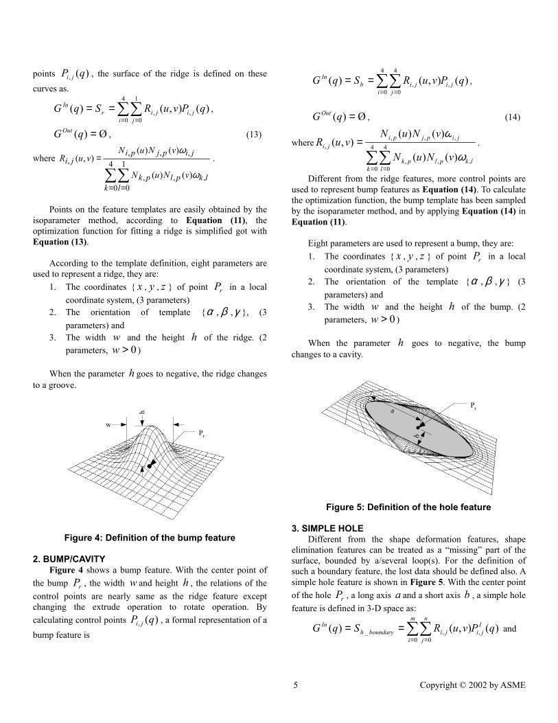
h0>w When the parameter h goes to negative, the bump

changes to a cavity. When the parameter goes to negative, the ridge changes

to a groove. h

Prab

h

Pr

w

Figure 5: Definition of the hole feature

3. SIMPLE HOLE Figure 4: Definition of the bump feature Different from the shape deformation features, shape

elimination features can be treated as a “missing” part of the surface, bounded by a/several loop(s). For the definition of such a boundary feature, the lost data should be defined also. A simple hole feature is shown in Figure 5. With the center point of the hole , a long axis a and a short axis b , a simple hole feature is defined in 3-D space as:

rP

2. BUMP/CAVITY

Figure 4 shows a bump feature. With the center point of the bump , the width and height , the relations of the control points are nearly same as the ridge feature except changing the extrude operation to rotate operation. By calculating control points , a formal representation of a bump feature is

w

,Pi

h

)(qj ∑∑= =

==m

i

Iji

n

jjiboundaryh

In qPvuRSqG0

,0

,_ )(),()( and


∑∑= =

==e

s

Ots

f

ttscenterh

Out qPvuQSqG0

,0

,_ )(),()( . (15)

Free form surfaceRidge template

Hei

ght

Width

where and are piecewise rational basis functions.

),(, vuR ji ),(, vuQ ji

In the Equation, two control point sets and

are used to define a hole feature. To , the data

come from given template boundary where for G , the

is come from the interpolation of current data follow the “natural” shape.

)(, qP Iji

)q

)(qOut

)(, qPOts

tsOP ,

(G In

(a) Varying width and height of a ridge template

Here, eight parameters are used to define a hole as: 1. The coordinates { x , , } of point in a local

coordinate system, (3 parameters) y z rP

2. The orientation of the template {α , β ,γ } (3 parameters), and

3. The radius of long axis and short axis . (2 parameters, and b )

a0>

b0>a

Then, the optimization function of a hole is conform

Equation (11) and Equation (15), where the value of scalar coefficient λ is very important to the optimization procedure which will be discussed in the next section. (b) Width, height and the result of optimization function

0

10

20

30

40

50

60

70

80

1 101 201Steps

Opt

imiz

e fu

nctio

n (m

m)

EXPERIMENTS AND ANALYSIS In this section several numerical experiments are presented

in order to verify the proposed fitting theory. Sensitivity of parameters in different kind of features is analyzed especially for the scalar coefficient λ . Based on λ and other parameters, a searching strategy for optimization function can be specified.

The goal of the sensitivity analysis is to verify the

optimization function and find the best searching strategy. To shape deformation features, such as ridge, obviously the template should totally match the surface since G .

That is, in the optimization function, coefficient

Ø)( =qOut

λ need not to be specified. (c) Searching procedure of a ridge feature


Surfacecontaininga hole

Hole template

GOut(q)

GIn(q)

b a

XY

Free form surface

Ridge template

(d) A fitted ridge feature

(a) A hole template and a surface containing a hole Figure 6: Fitting a ridge feature to a freeform surface

Unit: mm

Optimize function

With ACIS and Open Inventor , the whole system is modeled by Visual C++ and the search procedures were conducted using the IMSL C numerical libraries. In Figure 6(a), a ridge template and a freeform surface containing a ridge feature was put in 3-D space with 6 fixed parameters (the center point position and the template orientation). By varying parameters width and height around the optimal position, the value of optimization function is shown in Figure 6(b). From the figure, it is very clear that there is only one minimum point (around width =2.0 height =2.5) near the center area. It shows that fitting procedures can be carried out with finding the best parameters of the optimization function.

w h

(b) Varying x and in a hole optimization function with yλ =0.5

Searching strategies based on the quasi-Newton method were discussed in the authors’ former work [18]. Four kinds of search strategies were applied in the search procedure, and the best strategy was to divide the search into three steps. In the first two steps, the position and the orientation of the base point were fitted, then all parameters were fitted simultaneously. In the current numerical experiments, the freeform surface containing a ridge feature was represented by 1440 points. The ridge template was sampled with 1369 points. First, the ridge template was put at an arbitrary position in 3-D space, then the above searching strategy was applied. Figure 6(c) shows the search procedure of a ridge feature. With a Pentium III 700MHZ computer, the optimizing procedure was completed after 208 steps in 5 minutes. In the results, the width of the fitted ridge is 1.82mm where the height is 2.27mm. Figure 6(d) shows the final graphical result of the fitted ridge.

Unit: mm

Optimize function

(c) Varying x and in a hole optimization function with y

λ =0.5


Unit: mm

Optimize function

a b

Free form surface

Hole Part of a ridge feature

(d) Varying and in a hole optimization function with a b

λ =1 (a) Surface containing a hole (1675 points)

01020304050607080

1 101 Steps

Opt

imiz

e fu

nctio

n (m

m)

Unit: mm

Optimize function

a b

(b) Searching procedures

Free form surfaceHole template

GOut(q)

GIn(q)

(e) Varying and in a hole optimization function with a bλ =0.5

Figure 7: Varying parameters in a hole optimization

function To a shape elimination feature [6], such as a hole, it is clear

that , and coefficient Ø)( ≠qGOut λ should be specified.

Figure 7 shows the relation between parameters and the values of the optimization functions with different λ . In Figure 7(a), the feature template and the freeform features were put in the optimal position in 3-D space. Varying parameters x and

along X axis and Y axis respectively, when y λ equals to 1, the optimization function generates many local minimums near the optimum, as shown in Figure 7(b). Local minimums will make the searching procedure much more difficult or even impossible. While λ is set to 0.5, the shape of the optimization function is greatly changed and the search procedure can be simply carried out since local minimums are removed from the optimization function as shown in Figure 7(c).

(c) Hole fitting result

Figure 8: Fit a hole that interfered by a ridge However, a small λ would cause some problems, such as

a slower optimization speed. By varying the long and short axis radius and respectively, the shape of the result of the optimization function with

a bλ =1 as Figure 7(d) is much

“sharp” than what is obtained with λ =0.5, see Figure 7(e). That is, the search procedure of optimization function with large λ is much easier and faster than with small λ in the area around the optimal position.


Current research is directed towards further reduction of the computational complexity of the shape matching. The extension to more complicated features is also being studied. Some limitations of current system were found in the fitting process. Figure 9 shows the fitting result of matching between a leaning bump feature and the existing bump template. It shows that more parameters (here is the vertex of the bump or leaning angle) should be added into the feature in order to make it more flexible where the searching strategy should be optimized as well.

So the best searching strategy for shape elimination features is that in the global area, a small λ must be used to find the possible solution area, where within this area, a large λ accelerates the search procedure. Figure 8 shows some results of fitting hole template to a freeform surface. In Figure 8(a), the source data of a complex surface is presented with 1695 points. In the freeform surface, a hole is located in the center where part of it intersects a ridge feature.

With the optimization function, by applying different λ in

the searching process, the procedure worked well with this complex feature and an approximate result was generated. Figure 8(b) shows the searching procedure, the final result of the matching is shown in Figure 8(c). The numerical result is a hole with radius of long axis =3.22mm, short axis

=1.80mm. Pattern center position a

b x = 6.00mm, = 15.94mm and = 68.01mm, pattern orientation

yz α = -

16.13°, β = -5.90° and γ = -0.12°.

ACKNOWLEDGMENTS The research described in this paper is supported by the

ICA project of Faculty of Design, Engineering and Production, Delft University of Technology. Assistance from the ICA team members is appreciated.

REFERENCES 1. Ingle K.A., Reverse Engineering, McGraw-Hill, New

York, 1994. 2. Vergeest J.S.M. and Horvath I., Parameterization of

freeform features, Proceeding of Shape Modeling International, IMA-CNR, IEEE, Piscataway, 20-29, 2001.

Free form surface

Bump template

3. Vergeest J.S.M. and Horvath I., Matching 3D freeform shapes to digitized objects and its applications in shape modeling, Proceeding of PEDAC2001, 7th International Conference on Product Engineering, Design and Control, Production Engineering Department, Alexandria University, Alexandria, 2001.

4. Vergeest J.S.M., Spanjaard S., Horvath I. and Jelier J.J.O., Fitting freeform shape patterns to scanned 3D object, Proceeding of DETC’ 00, ASME 2000 Design Engineering Technical Conference and Computer and Information in Engineering Conference, Baltimore, Maryland, September 10-13, 2000.

Figure 9: The fitting result of a leaning bump

5. Shah J.J. and Mantyla M., Parametric and featured

based CAD/CAM, Wiley-Interscience Publication, John Wiley Sons In., 1995.

CONCLUSION AND FUTURE WORKS A method of direct fitting freeform surface by defined

freeform feature templates is presented in this paper. By the definitions of two shape dissimilarity measures in full 3-D space, the optimization function is built based on the mean directed Hausdorff distance by which noisy and incomplete data samples are suppressed. With the adjustable scalar coefficient λ , the optimizing procedure was carried out and accelerated. Several simple free from features were analyzed and parameterized according to high-level parameters, that is, the designer can easily change the freeform surface shape with these parameters. With the digitalized feature templates, numerical experiments were systematically conducted using sampled freeform surfaces. Through the result and the sensitivity analysis, it shows that directly match freeform surface with 3-D digitalized freeform feature template can be used as a satisfied tool in freeform surface reconstruction.

6. Fontana M., Giannini F. and Meirana M., A freeform feature taxonomy, Proceeding of Eurographics ’99, 18 (3), 1999.

7. Varady T. and Martin R.R., Reverse engineering, Handbook of CAD.

8. Li C.L. and Hui K.C., Feature recognition by template matching, Computer & Graphics, 24, 569-583, 2000.

9. Spanjaard, S. Documentation of ridge fit application and its source code. Technical report, Faculty of Design, Engineering and Production, Delft University of Technology, Delft, 2000.

10. Rowe J., "Surface modeling". Computer Graphics Wold, 20(9), 47-52, 1997.

11. Wyvill G., McRobie D. and Gigante M., Modeling with features". IEEE Computer Graphics and Applications, 15(5), 40-46, 1997.



12. Cavendish J.C., Integrating feature based surface design with freeform deformation, Computer-Aided Design, 27( 9), 703-711, 1995.

13. Van Elsas P.A. and Vergeest J.S.M. "Displacement feature modelling for conceptual design". Computer-Aided Design, 30(1), 19-27, 1998.

14. Veltkamp, R.C. "Shape matching: similarity measures and algorithms", Proc. Shape Modeling International Conference, a. Pasko and M. Spagnuolo, Eds., Los Alamitos, IEEE, 2001, 188-197.

15. Hagedoorn M. and Veltkamp R.C., Reliable and efficient pattern matching using an affine invariant metric. International Journal of Computer Vision, 31(2/3), 203-225, 1999.

16. Vergeest, J.S.M., Spanjaard S. and Song Y., "Direct 3D pattern matching in the domain of freeform shapes". Proceeding of the WSCG'2002.

17. Piegl L. and Tiller W. The NURBS book, Springer pres, Berlin, 1996.

18. Spanjaard S. and Vergeest, J.S.M., Comparing different fitting strategies for matching two 3D point sets using a multivariable minimizer Proc. of the 2001 Computers and Information in Engineering Conference, DETC'01/CIE-21242, ASME, New York, 2001.

Reconstructing Freeform Surface With Parameterized Features

Documents

Transcript of Reconstructing Freeform Surface With Parameterized Features