Reconstructing last glacial changes in Atlantic meridional ...

HAL Id: tel-01235193https://tel.archives-ouvertes.fr/tel-01235193

Submitted on 29 Nov 2015

HAL is a multi-disciplinary open accessarchive for the deposit and dissemination of sci-entific research documents, whether they are pub-lished or not. The documents may come fromteaching and research institutions in France orabroad, or from public or private research centers.

L’archive ouverte pluridisciplinaire HAL, estdestinée au dépôt et à la diffusion de documentsscientifiques de niveau recherche, publiés ou non,émanant des établissements d’enseignement et derecherche français ou étrangers, des laboratoirespublics ou privés.

Reconstructing last glacial changes in Atlanticmeridional overturning rate using marine sediment

(231Pa/230Th)Pierre Burckel

To cite this version:Pierre Burckel. Reconstructing last glacial changes in Atlantic meridional overturning rate usingmarine sediment (231Pa/230Th). Oceanography. Université de Versailles-Saint Quentin en Yvelines,2014. English. �NNT : 2014VERS0051�. �tel-01235193�

https://tel.archives-ouvertes.fr/tel-01235193

https://hal.archives-ouvertes.fr

THESE

Présentée pour l’obtention du grade de

Docteur de l’Université de Versailles SaintQuentin en Yvelines

Spécialité : Paléoclimatologie et Paléocéanographie

par

Pierre Burckel

Thèse intitulée

Utilisation du rapport (231Pa/230Th) des sédiments marins pour

caractériser les changements de circulation océanique lors des

variations climatiques de la dernière période glaciaire

Dont la soutenance aura lieu le 28 novembre 2014, devant le jury composé de :

- Mme. Claire Waelbroeck Directrice de thèse

- Mme Jeanne Gherardi Codirectrice de thèse

- M. Sylvain Pichat Codirecteur de thèse

- M. Alex Thomas Rapporteur

- Mme Mary Elliot Rapporteur

- M. Joerg Lippold Examinateur

-M. Philippe Bousquet Professeur à l’UVSQ

LSCE/IPSL, Laboratoire des Sciences du Climat et de l’Environnement

(CEA-CNRS-UVSQ)

Domaine du CNRS – Avenue de la Terrasse – 91190 - Gif-sur-Yvette - France

A ma famille et aux copains

Remerciements

Je tiens à démarrer ce manuscrit (ou à le finir, question de point de vue) en remerciant

toutes les personnes qui m’ont aidé ou soutenu pendant cette thèse. Et en trois ans de

thèse, trois ans d’aventure professionnelle mais également personnelle, ces personnes

sont nombreuses. Je vais donc tâcher de n’oublier personne. Mais si, vous qui me lisez,

ne voyez pas apparaître votre nom ci‐dessous et que vous vous en sentez lésé, c’est

certainement que je vous dois beaucoup, et je vous en remercie.

Je souhaite remercier en premier lieu Claire Waelbroeck, ma directrice de thèse.

En effet, un doctorat commence par un sujet de thèse, et le sujet que Claire a élaboré

était passionnant. Il m’a permis d’utiliser un matériel et des méthodes géochimiques de

pointe, afin d’étudier une zone clef pour la compréhension du climat et de l’océan de la

dernière période glaciaire. Claire, ta rigueur et ta franchise m’ont permis de développer

ma réflexion scientifique et d’adopter une méthode de travail qui m’a été précieuse

notamment lors de ma collaboration avec d’autres laboratoires. Dans les hauts et les bas

de cette thèse, tu m’as toujours fondamentalement fait confiance et, pour tout cela, un

grand merci à toi.

Un grand merci également à mes co‐directeurs de thèse, Jeanne Gherardi et

Sylvain Pichat, qui assuraient, entre autres, la partie expérimentale de mon

encadrement, partie à laquelle, vous le savez, je porte un immense intérêt. C’est

notamment grâce à vous que j’ai pu mettre le pied dans la communauté du Pa/Th, où j’ai

rencontré des personnes passionnées. Jeanne, merci de m’avoir fait découvrir

l’enseignement et de m’avoir prodigué tes conseils et idées sur l’après thèse.

Au cours de cette thèse, j’ai eu la chance de travailler avec deux équipes :

Paléocean et Geotrac. Un grand merci aux membres de ces deux équipes. Je pense tout

d’abord à Matthieu Roy Barman, auprès de qui j’ai pu bénéficier de nombreux conseils

concernant la mesure du rapport Pa/Th au laboratoire. Merci pour ces longues

discussions et le temps que tu y consacrais, ainsi que pour le covoiturage vers Chevry

qui m’a bien économisé les pieds ! Merci à Edwige Pons‐Branchu pour ses conseils et sa

gentillesse. Et encore désolé d’être entré en salle blanche avec des sédiments ! Un grand

merci à Dominique Blamart, qui a toujours su trouver les mots pour me motiver.

Toujours un plaisir d’entrer dans le bureau de « Dominique et Hervé » ! Merci également

à Eric Douville pour son calme et ses conseils, en particulier dans l’utilisation des

spectromètres. Un grand merci à Frank Bassinot, pour sa bonne humeur communicative

et maintes fois communiquée, et pour m’avoir permis de participer à la mission

océanographique MONOPOL qui a été une des expériences les plus marquantes de ma

thèse. Merci à Elisabeth Michel et à Jean Jouzel pour leur gentillesse et leurs conseils sur

mon premier article, et à Jean‐Claude Duplessy pour ses critiques qui m’ont aidé à

améliorer mes articles et mon manuscrit de thèse. Un grand merci à Gulay pour son

soutien moral inconditionnel et évidemment pour son aide dans la reconnaissance de

ces petites bestioles que sont les foraminifères. Merci à Fabien pour sa bonne humeur et

ses nombreux conseils, que ce soit au niveau des mesures ou sur mon futur

professionnel et personnel. Un immense merci à François qui m’a appris à dompter le

Neptune (enfin quand il se laissait faire). François, ton calme et ta bonne humeur ont

probablement renforcé mon intérêt pour la spectrométrie, quoique ta blague « y a pas

de signal dans tes échantillons » m’ait fait perdre beaucoup de cheveux. Un grand merci,

Natalia, pour tes conseils et ta gentillesse, et pour m’avoir évité de perdre le reste de

mes cheveux lorsqu’au moment fatidique, mon ordinateur refusait d’afficher

correctement les power‐points. Un immense merci à Hélène également, avec qui c’était

toujours un plaisir de prendre le thé ou simplement de discuter. Merci, Aline, pour ta

réactivité et tes explications claires, Louise pour tout le travail que tu accomplis

(presque) toujours dans la bonne humeur, Lorna, toi qui es toujours prompte à aider les

autres. Merci à Evelyn Böhm avec qui ce fut un plaisir de travailler pendant ce dernier

mois au LSCE.

Merci aussi à Virginie, Jean‐Pascal, Jean‐Louis Reyss, Hélène Valladas, Evelyne

Kaltnecker.

Je tiens également à remercier les gens d’en haut, les gens de l’Orme : Masa

Kageyama et Didier Roche, Gilles Ramstein et Jean Claude Dutay. Merci à Christophe

Colin d’IDES avec qui j’ai pu troquer du matériel de labo grâce à certains recoupements

inattendus entre la mesure des isotopes du néodyme et celle du rapport Pa/Th.

Un grand merci aux membres de mon comité de thèse Luke Skinner et Joerg Lippold.

Votre venue était toujours une bouffée d’air frais sur mon travail, et j’ai pris

énormément de plaisir à travailler très régulièrement avec Joerg. Egalement merci aux

membres de mon jury de thèse, Mary Elliot, Alex Thomas Philippe Bousquet et (encore)

Joerg Lippold.

Ce travail de thèse n’aurait pas été possible sans une bonne ambiance au

laboratoire, sans des épaules auxquelles se tenir, sans les copains. Hugo le goal ultra

volant, Cindy et ses séances de yoga, Jens qui me rappelle le pays, Naoufel qui se cache

dans les buissons pour « prendre des photos d’oiseaux », Marion qui est née du mauvais

côté des Vosges, Elian le sauveur de violon. Et bien sûr un grand merci à mon collègue de

bureau, Romain. J’espère que les successeurs du bureau 307 apprécieront nos moments

de décontraction placardés sur les murs et sur la porte . Merci également aux thésards

partis plus tôt : Cécile, Flora, Romain, Thomas, Sandra, David, Qiong, Véronique. A ceux

qu’on voit moins souvent ou qui sont là depuis peu : Quentin, Alison, Lucie, Wiem.

Enfin, un grand merci à ma famille et aux copains d’enfance, de fac, d’Erasmus.

Votre confiance, vos conseils et vos encouragements sont les fondations de ce travail.

Table of contents

Thesis abstract ................................................................................................................................. 1

Résumé de la these .......................................................................................................................... 3

Résumé détaillé en français ......................................................................................................... 5

Introduction ................................................................................................................................... 15

Chapter 1: Thesis objectives and study area ....................................................................... 19 1.1 Thesis objectives .......................................................................................................................... 19 1.1.1 Oceanic circulation variability during the past 60 ka ................................................................. 19 1.1.2 Origin of the Dansgaard Oeschger variability ................................................................................ 21 1.1.3 Dansgaard Oeschger variability outside the high latitude North Atlantic ......................... 23

1.2 Sedimentary Pa/Th ......................................................................................................................... 25 1.2.1 Behavior of protactinium and thorium in the ocean. .................................................................. 25 1.2.2 Pa/Th as a tracer of deep‐water renewal rate ............................................................................... 26 1.2.3 Effect of particle type and flux .............................................................................................................. 27 1.2.3 a) Use of the sedimentary Pa/Th ratio as a proxy of particle type and flux ................................... 27 1.2.3 b) Acquisition of the sedimentary Pa/Th signal ......................................................................................... 28

1.3 Stratigraphy of the cores ............................................................................................................... 28 1.3.1 Influence of the Amazon .......................................................................................................................... 29 1.3.2. Study area and stratigraphy of the cores ........................................................................................ 31

Chapter 2: Methodology ............................................................................................................. 41 2.1 Opal measurements ........................................................................................................................ 42 2.1.1 Method ............................................................................................................................................................. 42 2.1.2 Calculation ..................................................................................................................................................... 43 2.1.3 Uncertainties ................................................................................................................................................. 45

2.2 233Pa, 236U and 229Th spikes ........................................................................................................... 46 2.2.1 233Pa spike milking from 237Np .............................................................................................................. 46 2.2.2 233Pa calibration ........................................................................................................................................... 46 2.2.3 236U and 229Th calibration ........................................................................................................................ 47

2.3 Measurement by massspectrometry and Pa/Th calculation .......................................... 48 2.3.1 Measurements by mass‐spectrometry .............................................................................................. 48 2.3.2 Pa/Th calculation ........................................................................................................................................ 52

2.4 Pa/Th sediment results and intercomparison ..................................................................... 53 2.4.1 Methodological recommendations for the analysis of sedimentary Pa/Th. ..................... 53 2.4.2 Supporting Information ........................................................................................................................... 76

Chapter 3 : Timing of Oceanic circulation changes in the Atlantic during the last glacial ............................................................................................................................................... 93 3.1 Introduction ...................................................................................................................................... 93 3.2 Atlantic Ocean circulation changes preceded millennial tropical South America

rainfall events during the last glacial ............................................................................................... 94 3.3 Supporting Information ............................................................................................................. 115 3.4 Additional elements of discussion .......................................................................................... 135

Chapter 4: Changes in the geometry and strength of the AMOC during the last glacial ............................................................................................................................................. 137 4.1 Introduction ................................................................................................................................... 137 4.2 Changes in the geometry and strength of the AMOC during the last glacial ............. 139 4.3 Supporting Information ............................................................................................................. 164

Chapter 5: Conclusion and perspectives ............................................................................. 175

5.1 Conclusion ....................................................................................................................................... 175 5.1.1 Dansgaard‐Oeschger interstadials ................................................................................................... 175 5.1.2 Heinrich Stadials ...................................................................................................................................... 176 5.1.3 Dansgaard Oeschger Stadials .............................................................................................................. 177 5.1.4 Mechanisms of climate variability .................................................................................................... 177 5.1.4 a) Difference between Dansgaard Oeschger and Heinrich Stadials ................................................ 177 5.1.4 b) Effect of the AMOC on Greenland temperatures ................................................................................ 178

5.2 Perspectives ................................................................................................................................... 178

LIST OF FIGURES AND TABLES ............................................................................................... 181

REFERENCES ................................................................................................................................. 189

1

Thesis abstract

The upper circulation cell of the Atlantic Meridional Overturning Circulation (AMOC)

plays an important role in the climate system as it transports heat from the tropical

Atlantic to the North Atlantic high latitudes. Understanding the precise relation between

AMOC and climate requires long‐term data extracted from natural climate archives (e.g.,

marine sediment records, ice cores, stalagmites, …), as instrumental time series are too

short and impaired by the difficulty of distinguishing natural variability from

anthropogenic change.

My thesis objective has been to reconstruct the vertical layout and strength of the water

masses constituting the AMOC during fast climate changes of the last glacial using

sedimentary Pa/Th, a proxy of water mass flow rate.

My study area is situated on the Brazilian margin, an area that is the locus of the western

boundary currents and therefore ideal to monitor changes in the AMOC. The sediment

cores I studied also recorded the precipitation increases associated with the southward

shifts of the Inter Tropical Convergence Zone (ITCZ) occurring during stadials of the last

glacial. Because both precipitation proxies and water mass flow rate proxies are

recorded in the same core, I was able to reliably assess the timing of the AMOC upper

circulation cell slowdown with respect to the southward shifts of the ITCZ. I find that the

AMOC upper circulation cell started to slowdown 1420 ± 250 (1σ) and 690 ± 180 (1σ)

years before the southward ITCZ shifts associated with Heinrich Stadial 2 and Heinrich

Stadial 4, respectively. Hence, my results confirm that a slowdown of the AMOC could be

the origin of the ITCZ shifts associated with Heinrich Stadials and provide the first

precise estimate of the phasing between these two climate variables. Based on these

results I propose a mechanism explaining the difference between Heinrich and

Dansgaard‐Oeschger stadials.

Using modeling results, I show that the Atlantic Ocean circulation during periods of

higher Greenland temperatures (interstadials) was markedly different from that of the

Holocene. Two overturning cells were likely active in the Atlantic Ocean: an upper

overturning circulation cell initiated by northern‐sourced deep water flowing

southward above ~2500 m depth at the equator, and a lower overturning circulation

cell initiated by southern sourced deep water flowing northward below ~4000 m depth

at the equator. The overturning rate of the upper overturning cell was likely lower than

that of present‐day North Atlantic Deep Water. At the onset of Heinrich Stadials, the

structure of the AMOC significantly changed, and southern‐sourced deep‐waters likely

dominated the equatorial Atlantic Ocean below 1300 m depth.

3

Résumé de la these

La cellule supérieure de la circulation méridienne de retournement de l’Atlantique

(AMOC) transporte de la chaleur depuis l’Atlantique tropical vers les hautes latitudes de

l’océan Atlantique Nord, jouant ainsi un rôle clé dans le système climatique. Comprendre

précisément les relations entre l’AMOC et le climat requiert l’analyse d’enregistrements

climatiques longs, issus d’archives naturelles (telles que les carottes sédimentaires

marines, carottes de glaces, stalagmites…) car les séries de données instrumentales sont

trop courtes et ne permettent pas de distinguer les variations climatiques naturelles de

l’influence anthropique.

L’objectif de ma thèse a été de reconstituer la structure verticale et la dynamique des

masses d’eaux constituant l’AMOC au cours des variations climatiques rapides de la

dernière période glaciaire à partir du rapport Pa/Th sédimentaire, un traceur de la

vitesse d’écoulement des masses d’eaux.

Ma zone d’étude est située sur la marge nord‐est du Brésil, une zone affectée par les

courants de bord ouest et donc idéale pour reconstituer la variabilité de l’AMOC. Les

carottes sédimentaires que j’ai analysées ont également enregistré les augmentations de

précipitations associées aux migrations vers le sud de la zone de convergence

intertropicale (ITCZ) survenant durant les stadiaires de la dernière période glaciaire.

Comme les variations de précipitation et de circulation océanique sont enregistrées

dans la même carotte, j’ai pu précisément estimer le délai entre le ralentissement de

l’AMOC et le déplacement vers le sud de l’ITCZ. Je trouve ainsi que le ralentissement de

la cellule supérieure de l’AMOC commence 1420 ± 250 (1σ) années avant le

déplacement vers le sud de l’ITCZ associé au « Heinrich Stadial » 2 et 690 ± 180 (1σ)

années avant celui associé au « Heinrich Stadial » 4. Mes résultats confirment donc qu’un

ralentissement de l’AMOC pourrait être à l’origine des migrations de l’ITCZ associées aux

« Heinrich Stadials » et fournissent une première estimation précise du décalage

temporel entre ces deux variables climatiques. Sur la base de ces résultats, je propose un

mécanisme expliquant les différences entre les « Heinrich Stadials » et les « Dansgaard‐

Oeschger Stadials ».

A partir de résultats de modélisation, je montre que la circulation océanique pendant les

périodes chaudes au Groenland (« interstadials ») était très différente de celle de

l’Holocène. Deux cellules de circulation étaient probablement actives dans l’océan

Atlantique : une cellule supérieure initiée par l’écoulement au‐dessus de 2500 m à

l’équateur d’une masse d’eau en provenance du nord et se dirigeant vers le sud, et une

cellule inférieure initiée par l’écoulement au‐dessous de 4000 m à l’équateur d’une

masse d’eau en provenance du sud et se dirigeant vers le nord. Le taux de

renouvellement de la masse d’eau profonde de la cellule supérieure était probablement

4

plus faible que celle de la masse d’eau actuellement formée dans les hautes latitudes de

l’océan Atlantique Nord. Au début des « Heinrich Stadials », la structure de l’AMOC a

significativement changé et des eaux en provenance du sud ont probablement dominé

l’océan Atlantique équatorial en‐dessous de 1300 m de profondeur.

5

Résumé détaillé en français

Au cours de la dernière période glaciaire, les températures de l’air au‐dessus du

Groenland ont oscillé à l’échelle du millénaire entre périodes chaudes (interstadiaires)

et périodes froides (stadiaires) (Johnsen et al., 1992). Chaque stadiaire est terminé par

une augmentation des températures de l’air de l’ordre d’une dizaine de degrés, atteinte

en quelques décennies seulement, et marquant l’entrée dans des conditions

interstadiaires (Kindler et al., 2014). Durant chaque interstadiaire, les températures de

l’air diminuent vers de nouvelles conditions stadiaires (températures minimales)

maintenues pendant plusieurs centaines d’années. Ces réchauffements abrupts

enregistrés dans la glace du Groenland sont appelés « évènements de Dansgaard‐

Oeschger » (Dansgaard et al., 1993).

Pendant certains stadiaires, des fragments lithogènes grossiers ont été déposés dans les

sédiments de l’Atlantique Nord. Ces débris ne pouvant être amenés dans l’océan ouvert

que par des icebergs, ils sont appelés « Ice Rafted Detritus » (IRD). Les épaisses couches

d’IRD déposées dans l’Atlantique Nord sont appelées « Heinrich Events » (HE) (Heinrich,

1988), et les stadiaires au cours desquels elles sont déposées sont appelés « Heinrich

Stadials » (HS). Au cours des derniers 60 milles ans (ka), cinq Heinrich Stadials sont

observés dans les sédiments de l’Atlantique Nord (HS1‐HS5). Les stadiaires non associés

à des évènements d’Heinrich sont appelés DO‐stadials et les interstadiaires de la

dernière période glaciaire sont appelés DO‐interstadials.

La variabilité millénaire décrite ci‐dessus est associée à d’importantes variations de la

circulation méridienne de retournement de l’Atlantique (Atlantic Meridional

Overturning Circulation, AMOC). En effet, pendant les Heinrich Stadials, des réductions

de l’intensité de circulation des masses d’eau profonde constituant l’AMOC sont

observées (Gherardi et al., 2005; McManus et al., 2004). De plus, la formation d’eau

profonde dans l’Atlantique Nord semble diminuer (Elliot et al., 2002; Vidal et al., 1997),

ce qui pourrait être lié à la diminution de la salinité des eaux de surface de l’Atlantique

Nord observée pendant ces périodes (Bard et al., 2000; Cortijo et al., 1997; Maslin et al.,

1995).

Etant donné que l’AMOC redistribue la chaleur des tropiques vers l’Atlantique Nord, les

variations climatiques rapides observées au cours de la dernière période glaciaire

pourraient être engendrées par des variations de l’AMOC (Broecker et al., 1985). Or, le

dernier rapport de l’IPCC (2013) conclut que l’intensité de l’AMOC a de très fortes

chances de diminuer dans le futur, suite au réchauffement climatique induit par les

émissions anthropiques de gaz à effet de serre. Il est donc important de comprendre la

6

dynamique de l’AMOC lors des variations climatiques rapides de la dernière période

glaciaire pour mieux prévoir l’évolution future du climat.

Mon premier objectif de thèse consiste à reconstituer la dynamique des masses d’eau

formant l’AMOC au cours des variations climatiques rapides de la dernière période

glaciaire. Pour ce faire, j’utilise le rapport (231Pa/230Th)xs,0 (rapport d’activité du

protactinium et du thorium non supportés par l’uranium lithogène et authigène, et

corrigés de la décroissance radioactive) des sédiments marins qui est un proxy assez

récent de l’intensité de circulation des masses d’eau (Francois, 2007; Yu et al., 1996).

Mon second objectif consiste à comprendre la relation entre les variations de l’AMOC et

les changements climatiques rapides de la dernière période glaciaire. Pour ce faire, je

crée un modèle d’âge (i.e. correspondance entre profondeurs dans la carotte et âge

calendaire) pour mes carottes sédimentaires qui est entièrement radiométrique et

indépendant de l’échelle d’âge des carottes Groenlandaise (Greenland Ice Core

Chronology, GICC05). Je compare ensuite les enregistrements Pa/Th de mes carottes aux

variations de température du Groenland et aux variations de précipitations dans les

tropiques.

Ma zone d’étude est la marge nord‐est du Brésil. Cette région est idéale pour étudier la

variabilité de l’AMOC. En effet, elle est affectée par les courants de bord ouest, et les

masses d’eaux constituant l’AMOC y circulent donc de manière intense (Schott, 2003).

De plus, le talus continental permet d’étudier des carottes sédimentaires à différentes

profondeurs et donc d’étudier différentes masses d’eau. Les carottes sédimentaires que

j’ai étudiées au cours de ma thèse (MD09‐3257, 04°14.69’S, 36°21.18’W, 2344m de

profondeur; MD09‐3256Q, 03°32.81’S, 35°23.11’W, 3537m de profondeur) ont été

prélevées par le NR Marion Dufresne, au cours de la mission océanographique

MD173/RETRO3.

Afin de pouvoir comparer le signal de circulation enregistré dans mes carottes avec

d’autres enregistrements climatiques, j’ai tout d’abord établi la chronologie la plus

précise possible pour les deux carottes de ma zone d’étude. Les fortes pluies issues de la

migration vers le sud de la zone de convergence intertropicale (Intertropical

Convergence Zone, ITCZ) au cours des stadiaires ont occasionné une augmentation de

l’apport d’éléments terrigènes à la marge brésilienne par rapport à la sédimentation

carbonatée (Jaeschke et al., 2007). Ces migrations sont donc visibles grâce aux

augmentations du rapport Ti/Ca mesuré par XRF (X ray fluorescence) dans les carottes

sédimentaires de la zone d’étude (Arz et al., 1998; Jaeschke et al., 2007). Les pics du

rapport Ti/Ca sont très utiles pour corréler entre elles les carottes sédimentaires de la

7

marge. Ainsi, le modèle d’âge de la carotte MD09‐3257 (~2300 m de profondeur) est

basé sur la corrélation de ses pics de Ti/Ca avec ceux d’une carotte voisine (GeoB3910,

04°14.7’S, 36°20.7’W, 2362 m de profondeur) bien datée par 14C. Afin de vérifier cette

corrélation, plusieurs dates 14C ont été mesurées directement sur la carotte MD09‐3257.

Pour obtenir le modèle d’âge le plus précis possible, la partie de la carotte au‐delà de 38

ka a été datée par corrélation de ses pics de Ti/Ca avec les excursions négatives de δ18O

de spéléothèmes des grottes de Botuvera et de Diamante (Andes tropicales) (Cheng et

al., 2013). En effet, une diminution du δ18O des spéléothèmes indique, comme une

augmentation du Ti/Ca, une intensification des précipitations au‐dessus de la zone

d’étude. J’ai corrélé la partie de la carotte au‐delà de 38 ka aux spéléothèmes, car, après

35‐40 ka, les datations 14C sont très peu fiables (Reimer et al., 2013). Or les

spéléothèmes sont datés par U‐Th et permettent donc d’augmenter la justesse et la

précision du modèle d’âge sur la partie inférieure de la carotte. J’ai vérifié la validité de

la corrélation entre carottes marines et spéléothèmes sur les intervalles de temps où la

datation de la carotte sédimentaire par 14C est précise.

J’ai établi le modèle d’âge de la carotte MD09‐3256Q (~3500 m de profondeur) par

datation 14C jusqu’à 27 ka. Après cette date, j’ai corrélé les pics de Ti/Ca associés à HS3,

HS4 et HS5 dans la carotte aux pics de Ti/Ca de la carotte GeoB3910.

Pour estimer l’intensité de circulation des masses d’eau, j’utilise le rapport Pa/Th

sédimentaire. Le protactinium et le thorium sont produits à taux constant par l’uranium

dissous dans l’eau de mer avec un rapport de production de 0.093 (Henderson and

Anderson, 2003). Ces deux éléments sont très réactifs vis‐à‐vis des particules, et leur

temps de résidence dans l’océan est donc très faible. Toutefois, le temps de résidence du

thorium dans l’océan (30‐40 ans) est plus faible que celui du protactinium (~200 ans)

(Francois, 2007)). Ainsi, alors que le thorium est très rapidement adsorbé sur les

particules, le protactinium a tendance à rester en phase dissoute. Dans l’océan

Atlantique où le temps de résidence des masses d’eau est faible (100‐275 ans, (Yu et al.,

1996)), le protactinium peut donc être exporté latéralement par advection. Plus le débit

d’une masse d’eau est grand, moins le protactinium sera adsorbé sur les particules qui

sédimentent, et le rapport Pa/Th du sédiment sous‐jacent sera inférieur au rapport de

production de 0.093. A l’inverse, au sein d’une masse circulant très lentement, le

protactinium ne sera pas exporté latéralement et finira adsorbé sur les particules. Le

rapport Pa/Th sédimentaire se rapprochera donc du rapport de production. Etant

donné que le rapport Pa/Th sédimentaire est à l’équilibre avec le rapport Pa/Th dissous

dans les 1000 m de la masse d’eau au‐dessus du sédiment (Thomas et al., 2006), il peut

être utilisé pour estimer l’intensité de circulation des masses d’eau dans l’océan

Atlantique. En effet, en étudiant le Pa/Th sédimentaire de carottes verticalement

8

distantes de ~1000 m, on peut reconstruire le taux de renouvellement de plusieurs

masses d’eau.

Le rapport Pa/Th sédimentaire en tant que proxy du taux de renouvellement des masses

d’eau a néanmoins des limites. En effet, le protactinium a une forte affinité pour l’opale.

Ainsi, dans les zones à forte production d’opale ou à forts flux particulaires, le

protactinium peut être rapidement soustrait à la colonne d’eau par adsorption sur les

particules. Ces zones sont souvent des marges influencées par des upwellings côtiers,

comme la marge Africaine. La faible concentration en protactinium dissous résultant de

la forte productivité sur les marges entraîne la diffusion du protactinium depuis les

zones de forte concentration de l’océan ouvert vers les zones de faible concentration de

la marge. Cet apport de protactinium augmente le rapport Pa/Th sédimentaire sans

variation de circulation océanique. L’influence de la variation du type et des flux de

particules sur le rapport Pa/Th sédimentaire doit donc être évaluée avant d’interpréter

le Pa/Th comme un proxy du taux de renouvellement des masses d’eau.

J’ai également mesuré le δ13C des foraminifères benthiques C. wuellerstorfi afin de

reconstituer la ventilation des masses d’eau profondes (Duplessy et al., 1988). Ces

mesures sont complémentaires des mesures Pa/Th qui reflètent le débit des masses

d’eau.

J’ai concentré mes mesures Pa/Th autour de HS2 et de HS4. J’ai choisi ces périodes car

elles sont caractérisées par des calottes de glace de volumes différents (Lambeck and

Chappell, 2001). En effet, les calottes de glace de l’hémisphère nord sont plus étendues

pendant HS2 que pendant HS4. Il est donc intéressant de voir si ces configurations

différentes peuvent avoir un impact sur l’AMOC. Mes mesures Pa/Th sont les premières

effectuées à haute résolution autour de HS4, et les premières à être effectuées autour de

HS2 à ~2300 m de profondeur. J’ai mesuré le δ13C de C. wuellerstorfi sur la carotte

MD09‐3256Q (~3500 m de profondeur). Le δ13C de la carotte GeoB3910 située à

proximité de la carotte MD09‐3257 (~2300 m) a été mesuré par un autre laboratoire

lors d’une étude précédente et mis à ma disposition dans le cadre du projet ESF RETRO.

Les mesures Pa/Th que j’ai effectuées sur la carotte MD09‐3257 montrent l’importante

variabilité du débit de la cellule supérieure de l’AMOC au cours de la dernière période

glaciaire. Les stadiaires sont associés à de fortes valeurs du Pa/Th, indiquant une

réduction de l’intensité de la circulation entre ~1300 et 2300 m de profondeur.

Malheureusement, la portion de carotte correspondant au milieu de HS2 est affectée par

une turbidite, et je n’ai pu mesurer le Pa/Th que pendant le début de l’événement. De

plus, les fortes valeurs de Pa/Th observées pendant HS4 pourraient n’être pas

uniquement liées à des variations de circulation et je n’ai donc pas interprété ces

valeurs. En effet, les fortes valeurs Pa/Th pendant HS4 semblent corréler avec les forts

9

flux terrigènes. Il se pourrait donc que l’augmentation du flux particulaire ait entraîné

une forte diminution de la concentration en protactinium dissous sur notre zone

d’étude, ce qui aurait pu provoquer une arrivée de protactinium depuis l’océan ouvert.

Cela aurait pu masquer les variations du Pa/Th liées à des variations de circulation. Les

variations du Pa/Th précédant et suivant HS2 et HS4 peuvent toutefois être

interprétées, ainsi que les variations du Pa/Th observées lors des DO‐stadials et DO‐

interstadials.

Les mesures Pa/Th que j’ai effectuées dans la carotte MD09‐3256Q présentent une

moins grande variabilité que celles de la carotte MD09‐3257. La principale variation se

situe au sein d’HS4 qui voit le Pa/Th augmenter de ~0.06 à ~0.08. Toutefois, étant

donné que ces fortes valeurs Pa/Th sont associées à de forts flux terrigènes, les mesures

dans HS4 pourraient n’être pas uniquement liées à des variations de circulation et je ne

les ai donc pas interprétées.

Les mesures du rapport Pa/Th sur la carotte MD09‐3257 (~2300 m de profondeur)

montrent un ralentissement de la masse d’eau circulant au‐dessus du site avant les pics

de Ti/Ca associés à HS2 et à HS4. Etant donné que les mesures de circulation océanique

et de précipitations sont effectuées dans la même carotte, je peux précisément

déterminer la distance entre le début de l’augmentation du rapport Pa/Th sédimentaire

et le pic du Ti/Ca. Je trouve ainsi que le Pa/Th commence à augmenter 9 cm avant le pic

de Ti/Ca associé à HS2 et 5 cm avant celui associé à HS4. J’ai converti ces intervalles de

profondeur en intervalles de temps à l’aide du modèle d’âge que j’ai développé. Je trouve

ainsi que le débit de la cellule de circulation supérieure de l’AMOC diminue 1420 ± 250

(1σ) années avant la migration de l’ITCZ associée à HS2, et 690 ± 180 (1σ) années avant

celle associée à HS4. Mes résultats confirment qu’un ralentissement de l’AMOC et une

diminution du transport de chaleur vers l’Atlantique Nord pourraient être à l’origine de

la migration de l’ITCZ vers le sud.

Ces résultats contrastent avec les résultats des modèles climatiques. En effet, bien que

ces derniers soient capables de reproduire une migration de l’ITCZ vers le sud suite à un

ralentissement de l’AMOC, ce déplacement se produit rapidement après le début du

ralentissement de la circulation (Kageyama et al., 2009). Cela pourrait être dû au fait que

l’AMOC atteint son intensité minimale rapidement après le début du ralentissement de

la circulation en réponse à un apport d’eau douce dans les zones de formation d’eau

profonde de l’Atlantique Nord. Une réponse plus lente de l’AMOC occasionnerait

probablement une migration plus tardive de l’ITCZ vers le sud.

Les variations de circulation océanique au cours des DO‐stadials sont bien visibles sur la

carotte de profondeur intermédiaire de la marge brésilienne. L’intensité du

10

ralentissement de la cellule de circulation supérieure de l’AMOC associée à ces stadiaires

semble moins importante que celle associée aux Heinrich Stadials. Le rapport Ti/Ca

montre également que les DO‐stadials sont associés à une plus faible augmentation des

précipitations tropicales. La baisse du débit de la branche supérieure de l’AMOC et la

diminution des températures au Groenland semblent survenir en phase avec les

variations de précipitations. L’absence de délai significatif entre diminution des

températures au Groenland et migration de l’ITCZ pourrait impliquer que des processus

atmosphériques contrôlent la position de l’ITCZ pendant les DO‐stadials. Toutefois, les

DO‐stadials sont également associés à un ralentissement de la cellule supérieure de

l’AMOC. Ainsi, je ne peux pas déterminer quel mécanisme est à l’origine de la variabilité

de l’ITCZ au cours des DO‐stadials.

Le délai entre la baisse d’intensité de l’AMOC et la migration de l’ITCZ est très différent

pour les Heinrich Stadials et les DO‐stadials, ce qui m’a amené à proposer le mécanisme

suivant. Pendant les Heinrich Stadials, une diminution initiale du débit de la cellule de

circulation supérieure de l’AMOC a pu engendrer un réchauffement des eaux de

subsurface dans les hautes latitudes de l’Atlantique Nord (Alvarez‐Solas et al., 2013;

Mignot et al., 2007). Ce réchauffement aurait ensuite déstabilisé les plateformes de glace

en bordure des calottes de glace continentales, entraînant ainsi le vêlage de la calotte

Laurentide (Alvarez‐Solas et al., 2013). L’apport d’eau douce lié aux icebergs issus de la

Laurentide aurait alors entraîné la diminution du débit de la cellule supérieure de

l’AMOC, entraînant ainsi une accentuation du réchauffement des eaux de subsurface.

Cette boucle de rétroaction positive aurait ainsi pu se poursuivre, entraînant le

déplacement de l’ITCZ de plus en plus loin vers le sud. En revanche, je propose que cette

boucle n’ait pas été activée au cours des DO‐stadials, rendant ainsi la variation du débit

de la cellule supérieure de l’AMOC et la migration de l’ITCZ vers le sud limitées. Les

Heinrich Stadials seraient donc caractérisés par des débâcles d’icebergs très

importantes en raison de la boucle de rétroaction positive, alors que les décharges

d’icebergs auraient pu être davantage limitées au cours des DO‐stadials. Le mécanisme

proposé est par ailleurs en accord avec la différence de quantité d’IRD observée dans

l’Atlantique Nord entre les Heinrich Stadials, caractérisés par de grandes quantités d’IRD

(les évènements d’Heinrich), et les DO‐stadials, caractérisés par des quantités d’IRD

limitées.

Afin de comprendre les variations de l’agencement vertical et du débit des masses d’eau

constituant l’AMOC au cours des variations climatiques rapides de la dernière période

glaciaire, j’ai comparé mes données Pa/Th à des valeurs Pa/Th simulées par un simple

modèle 2D en boîtes forcé par différentes fonctions de courant. Ces fonctions de

11

courants ont été générées par le modèle iLOVECLIM (Roche et al., 2014, in press) sous

différentes conditions climatiques. Ainsi, avec l’aide du δ13C benthique, la comparaison

des valeurs Pa/Th de mes carottes sédimentaires et de deux autres carottes de

l’Atlantique avec les résultats du modèle m’a permis de proposer une configuration de

l’AMOC en accord avec les données pendant les DO‐interstadials et les Heinrich Stadials

(HS2) de la dernière période glaciaire.

Mes résultats montrent que la configuration de l’AMOC durant les DO‐interstadials de la

dernière période glaciaire était différente de la configuration actuelle. Les eaux

profondes en provenance de l’Atlantique Nord circulaient au‐dessus de 2500 m de

profondeur au niveau de l’équateur, alors qu’actuellement, les eaux profondes en

provenance du nord (NADW) s’étendent de 1200 à 4000 m de profondeur (Schott,

2003). De même, j’ai pu estimer que le débit de cette masse d’eau au niveau de

l’équateur était de 2 à 10 Sv, ce qui est inférieur à l’intensité de circulation actuelle de

NADW, qui est de 23 ± 3 Sv (Ganachaud and Wunsch, 2000). La masse d’eau profonde en

provenance des hautes latitudes sud circulait vers le nord au‐dessous de ~4000 m de

profondeur, et vers le sud en tant que courant de retour entre ~2500 et 4000 m de

profondeur. J’ai estimé que le débit de cette masse d’eau était de 2 à 10 Sv. Cette

estimation est trop peu précise pour en déduire un éventuel changement par rapport à

l’intensité de circulation actuelle de l’eau abyssale antarctique (AABW, 6 ± 1.3 Sv

(Ganachaud and Wunsch, 2000)).

Mes résultats montrent que la configuration de l’AMOC au cours des Heinrich Stadials

est très différente de la configuration au cours des DO‐interstadials. En effet, lors des

Heinrich Stadials, la production d’eau profonde dans l’Atlantique Nord semble avoir

suffisamment diminué pour que cette masse d’eau ne soit plus clairement visible à

~2300 m de profondeur au niveau de l’équateur. Une masse d’eau en provenance du sud

pourrait donc dominer la colonne d’eau en‐dessous de 1300 m de profondeur. La

circulation entre 1300 et 2300 m de profondeur semble être très fortement ralentie,

voire stoppée. La masse d’eau en provenance du sud semble directement affecter la

carotte sédimentaire profonde, et pourrait occuper la partie inférieure de la colonne

d’eau des abysses jusque vers 3500 à 2500 m de profondeur. Les données disponibles

montrent qu’à 4500 m cette masse d’eau s’étendait au moins jusqu’à 35°N. Je n’ai

toutefois pas pu estimer son débit car la fonction de courant associée à un arrêt complet

de la production d’eau profonde dans l’Atlantique Nord ne reproduit pas exactement

mes données Pa/Th.

12

Mes données ne montrent pas de différence majeure entre HS2 et HS4, malgré le fait que

ces deux stadiaires soient caractérisés par des calottes de glace de volumes différents.

Dans les deux cas, la diminution de la circulation océanique précède la migration de

l’ITCZ. Bien que mes résultats aient permis de mieux comprendre la structure de

l’Atlantique équatorial au cours de HS2, les doutes émis sur la capacité du Pa/Th à

représenter la circulation océanique au cours de HS4 m’ont empêché de comparer la

géométrie et la force de l’AMOC au cours de ces deux périodes de temps. La seule

différence manifeste entre les deux stadiaires est le plus faible δ13C des DO‐interstadials

entourant HS2 par rapport à ceux entourant HS4. Toutefois, cette différence pourrait

être due à l’évolution de la biosphère continentale accompagnant le développement

progressif des calottes de glace depuis l’entrée en glaciation jusqu’au dernier maximum

glaciaire (~21 ka) (Duplessy et al., 1988; Lambeck and Chappell, 2001). Rien ne nous

permet donc de dire que la circulation océanique dans l’Atlantique et son lien avec le

climat étaient significativement différents entre HS4 et HS2.

Finalement, la comparaison de mes résultats avec l’enregistrement de la température au

Groenland montre que les températures du Groenland sont restées inchangées alors que

la cellule de circulation supérieure de l’AMOC était ralentie durant HS2. Cela implique

que l’impact de l’apport de chaleur océanique sur les températures du Groenland est

modulé par d’autres processus. D’une part, des études de modélisation montrent que la

glace de mer pourrait être un agent important de la variabilité des températures au

Groenland, et pourrait agir comme un isolant sur ce dernier, empêchant ainsi une

diminution de l’apport de chaleur océanique de réduire davantage les températures

groenlandaises (Kaspi et al., 2004; Li et al., 2010).

D’autre part, les études de modélisation montrent qu’une diminution de l’apport de

chaleur par les océans pourrait être compensée par une augmentation du transport de

chaleur par l’atmosphère (Kageyama et al., 2009; Shaffrey and Sutton, 2006).

En conclusion, je montre au cours de cette thèse que le débit et la distribution des

différentes masses d’eau constituant l’AMOC ont significativement varié au cours des

variations climatiques rapides de la dernière période glaciaire. Pendant les DO‐

interstadials, deux cellules de circulation étaient actives au‐dessus et au‐dessous de

2500 m, avec un débit de la cellule supérieure inférieur au débit actuel de NADW. La

diminution du débit de la masse d’eau supérieure associée aux Heinrich‐Stadials

intervient 500 à 1700 ans avant la migration vers le sud de l’ITCZ. Ainsi, un

ralentissement de la cellule supérieure de l’AMOC pourrait avoir causé le déplacement

de la zone de convergence intertropicale. Enfin, au cours des Heinrich Stadials, la

convection d’eau profonde dans l’Atlantique Nord était probablement limitée, et l’océan

13

Atlantique était dominé par une masse d’eau en provenance du sud au moins en‐dessous

de 1300 m de profondeur.

15

Introduction

Deep ice core drilling revealed millennial scale Greenland air temperature variability

over the course of the last glacial, referred to as Dansgaard‐Oeschger variability (Fig. 1)

(Dansgaard et al., 1993; Kindler et al., 2014). DO events are characterized by rapid

transitions from cold (stadial) to warm (interstadial) conditions. In marine sediment

cores from the mid‐high latitude North Atlantic, sea surface temperatures estimates

display a similar variability, with cold sea surface temperatures (SST) occurring during

DO stadials (Bard et al., 2000; Bond et al., 1993; Elliot et al., 2002; Sachs and Lehman,

1999). During some of these stadials, layers of coarse lithic fragments occur in mid‐high

latitude North Atlantic marine sediment cores (Bond et al., 1992). The coarse grains

found within these layers were transported by icebergs before being deposited in

oceanic sediments and are termed Ice Rafted Detritus (IRD). Anomalously thick layers of

IRD are called Heinrich Events and the stadials during which they occur are called

Heinrich Stadials (Heinrich, 1988). Evidences for climatic variability associated with

Heinrich and Dansgaard‐Oeschger events are not limited to the high latitude North

Atlantic and can be found worldwide (Voelker, 2002).

Figure 1 : Greenland air temperatures of the last 20‐50 ka (Kindler et al., 2014). Numbers indicate

Dansgaard‐Oeschger interstadials and HS indicates Heinrich Stadials.

Heinrich stadials are accompanied by decreased flow rate of the deep water

masses contributing to the Atlantic Meridonal Overturning Circulation (AMOC)

(Gherardi et al., 2005; McManus et al., 2004) and by reduced deep water formation in

the high latitude North Atlantic (Elliot et al., 2002; Vidal et al., 1997). The AMOC is the

meridional component of the Atlantic circulation (Fig. 2). (Kuhlbrodt et al., 2007). It

2"

3" 4"

5"6"

7" 8"

9"

10"11"

12"

HS2" HS3" HS4" HS5"

Age"(ka)"

Temperature"(°C)"

=60"

=50"

=40"

=30"

=20"

20" 25" 30" 35" 40" 45" 50"

16

consists of two overturning cells: the upper cell is initiated by deep convection in the

Nordic seas and the lower cell is initiated by deep convection in the Southern Ocean. The

surface circulation of the upper circulation cell is responsible for the transport of heat

and salt from the tropical Atlantic towards the high latitude North Atlantic. Hence, it has

been hypothesized that decreased inter‐hemispheric heat transport related to a

reduction of the AMOC strength could be at the origin of the climate variability observed

in Greenland ice cores (Broecker et al., 1985).

The last IPCC report (AR5) concluded that a slowdown of the AMOC is very likely

in the future, as a consequence of the warming induced by greenhouse gas emissions

due to human activities. Although modern climate could respond differently to an AMOC

slowdown than that of the last glacial, studying the AMOC of the last glacial and its links

with abrupt climate shifts could help improving current climate models and hence

predicting future climate change.

Figure 2 : Sketch of the Atlantic Meridional Overturning Circulation (AMOC) from (Kuhlbrodt et al., 2007). Blue arrows indicate the approximate flow direction of NADW (North Atlantic Deep Water) and AABW

(Antarctic Bottom Water), the northern and southern sourced deep water masses initiating the upper and

lower overturning cells of the AMOC respectively.

In this thesis, I reconstruct the dynamic of the AMOC during warm and cold

periods associated with the DO variability. In order to do that, I use the sedimentary

Pa/Th ratio, a relatively recent proxy that can record water masses renewal rates

(Francois, 2007; Yu et al., 1996). I also study the relationship between AMOC and fast

climate changes of the last glacial. My study area is situated on the Brazilian margin, a

region affected by strong western boundary currents and therefore by the main water

17

masses constituting the AMOC (Schott, 2003). The sedimentary Pa/Th ratio in this

region was shown to reflect present day oceanic circulation (Lippold et al., 2011).

In Chapter 1, I present the current knowledge on the strength and layout of the

water masses constituting the AMOC, and their links with climate of the past 60 cal ky

BP (ka hereafter). I also present the objectives of this thesis, which aim at understanding

some actively discussed aspects concerning the configuration of the water masses

constituting the AMOC and their relationship with climate of the last glacial. I also

present the current knowledge of the sedimentary Pa/Th ratio in the Atlantic. Finally, I

detail my study area and the stratigraphy of my sediment cores, which has been crucial

in my choice of the fast climatic events to study.

Chapter 2 provides details about the methods I implemented at LSCE. The core of

this chapter is one of my three research papers, intended for submission in Analytical

Chemistry. This article is an intercomparison of sedimentary Pa/Th methods, and

provides advices for Pa/Th measurements and 233Pa spike calibration. Within the frame

of this thesis, it provides an assessment of the quality of the data that I produced.

In chapter 3, I assess the timing of AMOC change with respect to shifts of the Inter

Tropical Convergence Zone. In order to that, I build an age model for the sediment cores

that is entirely radiogenic. Hence, as this age model is independent from the ice core

GICC05 age scale, I compare AMOC changes to temperature changes in Greenland. This

study is the subject of an article that was submitted to Nature Geoscience and

Proceedings of the National Academy of Sciences, but that was not accepted with 1/3

and 1/2 positive reviews. It is now intended for submission in Geophysical Research

Letters.

In chapter 4, I compare the Pa/Th data in the sediment cores of this study and in

other Atlantic cores to Pa/Th values simulated using a 2D box model forced by various

streamfunctions. It allows me to infer possible states of the AMOC during different

climate periods of the last glacial. This article, currently in preparation, is intended for

submission to Climate of the Past.

The last chapter summarizes all the results that arise from this thesis. It also

provides perspectives for future work aiming at testing the hypotheses I emitted, and at

providing further insights into our understanding of the AMOC and its relation with last

glacial climate.

19

Chapter 1: Thesis objectives and study area

1.1 Thesis objectives

In this section, I present the current knowledge on the structure of the AMOC during the

past 60 cal ky BP (ka hereafter) and its relationship with climate. I separate my

presentation into different topics, and detail my thesis objectives related to these topics

at the end of each associated subsection (1.1.1‐1.1.3).

1.1.1 Oceanic circulation variability during the past 60 ka

During the last 60 ka, the Atlantic Meridional Overturning Circulation (AMOC) shifted

between different states (Alley and Clark, 1999; Rahmstorf, 2002). At present, deep

convection in the high latitude North Atlantic mainly occurs in the Greenland,

Norwegian, Island and Labrador seas (Dickson and Brown, 1994; Reid, 1994) by brine

rejection from sea ice formation, heat loss to the atmosphere and cyclonic wind induced

vertical mixing (Kuhlbrodt et al., 2007). The deep water formed is called North Atlantic

Deep Water (NADW), and overflows the Greenland‐Scotland ridge into the Atlantic

before flowing southwards towards the Southern Ocean. NADW salinity is high (34.8‐35

‰) (Emery, 2001) and its nutrient content is low, as reflected by the high δ13C (0.9‐1.1

‰) of its dissolved inorganic carbon (DIC) (Kroopnick, 1985). NADW flows in the

Atlantic Ocean between 1.2 and 4‐5 km depth (Schott, 2003). The Antarctic Bottom

Water (AABW) is a cold water mass of low salinity (‐0.9‐1.7°C, 34.64‐34.72 ‰) (Emery,

2001) mainly formed during austral winter by deep convection in the Weddell Sea

(Dickson and Brown, 1994). It enters the North Atlantic below 4000 m depth, through

the equatorial path (Schott, 2003), and its influence can be seen as far north as 50°N.

The Antarctic Intermediate Water (AAIW) is formed in the vicinity of the Antarctic polar

front (Lynch‐Stieglitz et al., 1994) and flows northwards between 550 and 1200 m

depth along the South American margin, at least up to 16°N where it is disturbed by the

occurrence of the Mediterranean overflow waters (Lankhorst et al., 2009; Reid, 1994;

Viana et al., 1998). As for AABW, AAIW is rich in nutrients (Reid, 1994) and its salinity is

low (33.8‐34.8 ‰) (Emery, 2001).

During the Last Glacial Maximum (LGM), deep convection appears to have been still

active but shifted south of Iceland, on the Rockall plateau (Vidal et al., 1997). At that

time, the deep water mass formed in the high latitude North Atlantic could have been

active above 2000 m depth, down to 10°S, and is therefore named Glacial North Atlantic

20

Intermediate Water (GNAIW) (Alley and Clark, 1999; Boyle and Keigwin, 1987; Curry

and Oppo, 2005; Duplessy et al., 1988; Gherardi et al., 2009; Oppo and Lehman, 1993).

At greater depth, poorly ventilated northward flowing waters originating from the

Southern Ocean probably dominated the Atlantic Ocean up to 50°N (Alley and Clark,

1999; Boyle and Keigwin, 1987; Curry and Oppo, 2005; Duplessy et al., 1988; Oppo and

Lehman, 1993). AAIW became colder and less saline, as it received more contribution

from the Indian Ocean (Lynch‐Stieglitz et al., 1994) and its influence spread at least up

to the Demerara rise (Huang et al., 2014), but not as far north as the Caribbean Sea

(Straub et al., 2013).

During Heinrich Stadials 1 to 5, the low δ13C values in the northern North Atlantic Ocean

could indicate that deep convection was weakened, if not stopped (Elliot et al., 2002;

Vidal et al., 1997). A deep convection zone was however potentially still active south of

Iceland during HS4, within the present day polar and subtropical modal water formation

zone (Vidal et al., 1997). The apparent decreased deep convection during Heinrich

Stadials 1 to 5 could be related to the release of icebergs in the Atlantic Ocean from the

Nordic ice sheets (Hemming, 2004), which is accompanied by decreased salinity (Bond

et al., 1993; Labeyrie et al., 1995; Maslin et al., 1995) and temperatures (McManus et al.,

1999; Vautravers et al., 2004) in high latitude North Atlantic surface waters (see section

1.1.2).

During Heinrich Stadials, the influence of the AMOC upper circulation cell decreased,

which is visible through the increased influence of southern sourced water masses in

the northern North Atlantic, deduced from paleo‐nutrient proxies (Elliot et al., 2002;

Oppo and Lehman, 1995), but also from the reduced overflow of Nordic seas into the

Atlantic Ocean inferred from the presence of Atlantic benthic species at the Faeroe

margin (Rasmussen et al., 1996).

Moreover, several studies using the sedimentary Pa/Th ratio show that the AMOC

strength decreased below 2000 m depth in the northern North Atlantic, but these

studies are restricted to Heinrich Stadial 1 and the Younger Dryas (Gherardi et al., 2005;

Gherardi et al., 2009; McManus et al., 2004). However, a few studies show that a shallow

circulation cell could have been still active above 2000 m depth during Heinrich Stadials

1‐3 (Gherardi et al., 2009; Lynch‐Stieglitz et al., 2014), meaning that Heinrich Stadials

may not be associated with a complete shutdown of the AMOC upper circulation cell.

Hence, further progress needs to be made regarding the configuration and intensity of

the water masses constituting the AMOC during Heinrich Stadials of the last glacial.

21

The extent of AAIW during Heinrich Stadials is still under discussion. Some studies claim

that it increased during these periods in the Atlantic (Mangini et al., 2010; Pahnke et al.,

2008) and in the Pacific (Pena et al., 2013), while others argue the opposite (Huang et

al., 2014).

Most of our knowledge about the AMOC during Heinrich Stadials is based on paleo‐

nutrient proxies. Moreover, the few reconstructions of the AMOC strength are focused

on HS1 and the Younger Dryas. My first thesis objective is therefore to reconstruct the

dynamic of the AMOC over some rapid climate variations of the last glacial, using the

sedimentary Pa/Th ratio (Chapter 3 and 4, (Burckel et al., 2014 a, in prep.; Burckel et al.,

2014 b, in prep.)).

1.1.2 Origin of the Dansgaard Oeschger variability

Different mechanisms have been proposed to explain the abrupt Greenland air

temperature changes that occurred during the last glacial. Changes in the intensity of the

Atlantic Meridional Overturning Circulation (AMOC), which exports heat and salt from

the equator towards the high latitude North Atlantic (Talley et al., 2003), were

suggested to drive Greenland temperature oscillations (Broecker et al., 1990; Broecker

et al., 1985). A decreased AMOC intensity could be at the origin of Dansgaard Oeschger

(DO) and Heinrich stadials, while DO interstadials could be related to increased

meridional heat export to the northern hemisphere by the resumption of an active

oceanic circulation in the Atlantic (Broecker et al., 1985). A decreased intensity of the

AMOC and an increased influence of Southern Ocean waters has been shown to occur

during Heinrich (Elliot et al., 2002; Gherardi et al., 2005; McManus et al., 2004; Vidal et

al., 1997) and DO stadials (Charles et al., 1996; Kissel et al., 1999) in agreement with the

hypothesis of an AMOC influence on Greenland temperatures. A slowdown of the AMOC

could result from the decreased sea surface salinity (SSS), which is recorded in the

North Atlantic down to the sub‐tropics (~38°N) during Heinrich Events (Bard et al.,

2000; Cortijo et al., 1997; Maslin et al., 1995). Indeed, increased freshwater input into

the high latitude North Atlantic Ocean could increase the buoyancy of surface waters

and prevent deep convection and formation of deep northern sourced waters, therefore

decreasing the AMOC strength. Using fully coupled climate models, a freshwater forcing

in agreement with northern North Atlantic salinity proxies during HE4 indeed induces a

shutdown of the AMOC (Roche et al., 2004), which results in a drop of northern North

Atlantic temperatures (Kageyama et al., 2009). A freshwater input in the northern North

Atlantic could therefore trigger an AMOC slowdown that would in turn lead to a

decrease in air temperatures above Greenland.

22

Melting of icebergs released into the North Atlantic during Heinrich Events could

have been at the origin of the freshwater input required to disrupt the AMOC. Different

hypotheses exist to explain Heinrich Events. They could be the consequence of

jökulhlaups (major flood) from a Hudson Bay lake, of ice sheets collapse because of basal

melting by geothermal heat (binge purge mechanism), or of ice shelf build‐up/collapse

(see (Hemming, 2004) for a review). However, some recent studies suggest that, rather

than causing the AMOC slowdown, Heinrich Events could be a consequence of the

reduced overturning circulation (Alvarez‐Solas et al., 2013). Indeed, a warming of

subsurface waters is observed in the high latitude North Atlantic during Heinrich

Events, which could be due to a cessation of deep convection and increased stratification

(Marcott et al., 2011). Modelling experiments show that a subsurface warming could

have destabilized the ice shelves, leading to the iceberg release observed during

Heinrich Events, so that a decrease of the AMOC could have induced the Heinrich Events

(Alvarez‐Solas et al., 2013). Such an idea is comforted by a study from the apparent lead

of water mass proxies, indicating increased Southern Ocean water influence, with

respect to Heinrich Events (Gutjahr and Lippold, 2011). Moreover, increased buoyancy

of subsurface waters could lead to a disruption of oceanic stratification and to the

emergence of warm waters in the high latitude North Atlantic (Rasmussen and

Thomsen, 2004). The amounts of heat released to the atmosphere could in turn lead to

the fast temperature rise associated with DO interstadials. Hence, it is yet unclear

whether AMOC slowdowns observed during the last glacial are the cause or the

consequence of Heinrich Events.

Also, based on spectral analysis of the GISP2 δ18O signal, DO events have been

suggested to occur with a 1470 year periodicity (Schulz, 2002). Although no orbital or

solar forcing presents such a periodicity, it was shown that a combination of centennial

scale solar cycles and its effects on the AMOC could result in 1470 years cyclical

temperature oscillations in Greenland (Braun et al., 2005). However, such a periodicity

is for now rejected from spectral analysis on Greenland data in the most recent GICC05

NGRIP age scale (Ditlevsen et al., 2007).

Some recent studies based on shallow North Atlantic sediment cores suggest that

the AMOC did not slow down during HE1‐3 (Gherardi et al., 2009; Lynch‐Stieglitz et al.,

2014). Instead, there could have been an active overturning cell operating at mid water

depths (>2000 m) at that time. These results challenge the classical idea that variations

in Greenland temperatures are related to variations in the intensity of the AMOC, and

alternative hypotheses may therefore be necessary to explain the DO variability.

Sea ice through its effect on albedo and insulation could have triggered DO like

events with only a weak AMOC variability (Kaspi et al., 2004). Indeed, a slight reduction

of the AMOC triggered for instance by ice sheet discharge into the high latitude North

23

Atlantic Ocean would allow sea ice expansion. Because of the positive feedback caused

by increased surface albedo, ocean and atmosphere temperature would cool, leading to

rapid sea ice expansion. The expansion of sea ice would be limited by its insulation effect

on the ocean. The heat and salt stored in the tropics would then start diffusing towards

the high latitude North Atlantic, causing sea ice to melt rapidly because of the positive

feedback resulting from decreased albedo and insulation. This effect would rapidly

warm the atmosphere and could lead to the DO variability observed in Greenland

temperatures with a minor change of the AMOC.

Moreover, sea ice could have acted as a positive feedback through its effect on the

position of the polar jet (Li et al., 2010). Indeed, during cold periods above Greenland,

the Inter Tropical Convergence Zone shifted southwards (see section 1.1.3) which could

have led to a southward shift of the polar jet, resulting in a decreased transport of heat

by the atmosphere into the North Atlantic region and to enhanced sea ice formation.

My second thesis objective is to increase our understanding of the relationship

between AMOC and climate variations of the last glacial, and the mechanisms through

which they interact. In order to do that, I deploy two strategies (see also section 1.1.3).

My first strategy is to compare changes in AMOC intensity to Greenland temperatures

to assess the effect of reduced or intensified oceanic circulation on Greenland climate. I

therefore build an age model independent from the GICC05 time scale to compare the

timing and extent of the Atlantic circulation changes with respect to fast Greenland

temperature variations of the last glacial (Chapter 3, (Burckel et al., 2014 a, in prep.)).

1.1.3 Dansgaard Oeschger variability outside the high latitude North Atlantic

During the last glacial, temperature oscillations are also observed in Antarctic ice cores

δ18O and δD records. Temperatures signals from the northern and southern hemisphere

ice cores are out of phase (Blunier and Brook, 2001; EPICA, 2006). This observation led

to the formulation of the bipolar seesaw concept (Stocker, 1998). In this concept,

southern and northern hemispheres have a temperature response to an AMOC variation

of opposite sign. Active oceanic circulation results in the transport of heat towards the

high latitude North Atlantic. This leads to Greenland warming and Antarctic cooling.

During AMOC slowdowns, heat is retained south of the equator, and leads to a warming

of the southern tropical Atlantic and to a cooling of the North Atlantic. Such a concept is

reproduced by climate models (Kageyama et al., 2009) and is able to produce the abrupt

warming and slow cooling characteristic of DO events in Greenland (Stocker and

Johnsen, 2003). Indeed, when the AMOC resumes, the heat stored at low latitudes is

abruptly transferred to the high latitude northern Atlantic, thereby producing an abrupt

24

warming. A slow AMOC decrease is then able to progressively lower the heat supply and

decrease Greenland temperatures.

Last glacial climate variability was also shown to impact tropical precipitation. During

cold stadials such as Heinrich stadials and, to a lesser extent, during DO stadials, the

reflectance and Ti/Ca signals recorded in northern tropics sediment cores (Cariaco

basin and Arabian sea (Deplazes et al., 2013; Lea et al., 2003)) increased and decreased

respectively, indicating lower terrigenous input to the cores’ sites. At the same time, the

δ18O signal of speleothems from the Hulu cave in China increased (Wang et al., 2001).

Both these variations are interpreted as a decrease in northern tropics precipitation,

related to a southward shift of the Inter Tropical Convergence Zone (ITCZ). Indeed, at

the same time, the southern tropics experienced increased precipitation, which are seen

in marine sediment cores from the Brazilian margin (Jaeschke et al., 2007) as well as in

South American speleothems (Cheng et al., 2013). Climate models are able to reproduce

these ITCZ shifts by simulating a cold SST anomaly in the northern tropics. Indeed, the

ITCZ lies above warm waters, where air convection and intense precipitation occurs

(Hastenrath, 2011) so that a cold anomaly in the northern tropics induces a shift of the

tropical rain‐belt towards the warmer southern tropics. Modelling experiments can

produce a cold SST anomaly in the northern tropics by two different mechanisms. In the

first mechanism (Chiang and Bitz, 2005), extended sea ice or ice sheet cover in the

northern high latitudes cools and dries the atmosphere. This cooling and drying

propagates to the entire northern high and mid latitude by atmospheric transport and

mixing. In the tropics, northeastern trade winds are intensified because of the cool mid‐

latitude ocean, which leads to further evaporation and cooling and pushes the SST

anomaly southwards leading to a southward shift of the ITCZ. In the second mechanism

(Kageyama et al., 2010), an AMOC slowdown causes the northern tropical ocean to cool

and southern tropical ocean to warm, as predicted by the bipolar seesaw concept. The

ITCZ therefore shifts towards the warmer southern tropics.

My second strategy to understand the relationship between AMOC and climate

variability of the last glacial is to analyse the phasing of AMOC circulation changes and

ITCZ shifts. Because the sediment cores I use in this study are situated on the Brazilian

margin, precipitation and circulation proxies are recorded in the same core, which

allows me to reliably assess the time interval between the beginning of the AMOC

slowdown and the ITCZ shift (Chapter 3, (Burckel et al., 2014 a, in prep.)).

25

1.2 Sedimentary Pa/Th

1.2.1 Behavior of protactinium and thorium in the ocean.

231Pa and 230Th production in the ocean results from the decay of dissolved 235U and

234U, respectively. Under oxic conditions, uranium is very soluble (Dunk et al., 2002;

Weyer et al., 2008). Its residence time in the Ocean is therefore very large (~500 ky)

(Weyer et al., 2008). The mixing time of the ocean is comparatively very short (from 1‐

1,6 ky) (Broecker and Peng, 1982) so that uranium concentration in the ocean is

uniform and proportional to salinity (Dunk et al., 2002). The isotopic composition of

uranium is also uniform, with a measured 234U/238U activity ratio of 1,1466 (Robinson et

al., 2004b) and a 235U/238U activity ratio of 0,04604 (Francois, 2007). Hence, we can

calculate that the protactinium and thorium are produced at a constant activity ratio of

0.093 in the ocean:

P!"

P!! =

λ!"#× A!"#

A!"#

λ!"#×A!"#

A!"#

=2,12 ×10!!× 0,04604

9,20 ×10!!× 1,1466≅ 0,093

where λ231 and λ230 are the decay constant of 231Pa and 230Th respectively (Audi et al.,

2003).

Protactinium and thorium have a different behavior in the ocean. Both elements are

very particle reactive and are quickly adsorbed on particles. They can consequently be

removed from the water column by settling to the seafloor. Adsorption of Pa and Th on

particles and subsequent removal to the seafloor is termed scavenging (Henderson and

Anderson, 2003) and is particularly active for Pa and Th, as reflected by their low mean

residence time in the ocean (~200 years for Pa and 30 years for Th) (Yu et al., 1996).

Dissolved and particulate Th concentrations have been shown to broadly increase with

depth at several locations (Fig. 1) (Henderson and Anderson, 2003). A linear increase of

dissolved concentrations implies the existence of reversible scavenging, i.e. the Th

adsorbed on the particulate fraction continuously exchanges with the dissolved pool

(Francois, 2007). The protactinium also shows such a trend in some water profiles, but

this is very rare because of its longer residence time with respect to scavenging, which

allows protactinium to be transported horizontally (Fig. 1) (Choi et al., 2001). Indeed,

with increasing depth and therefore increasing residence time, dissolved and particulate

protactinium depth‐profiles tend to deviate from linearity because of the increased

protactinium export caused by advection in the Atlantic Ocean (Fig. 1).

26

Figure 1.1 : Dissolved 231Pa and 230Th profiles in the equatorial Atlantic (st.3 and st.4) from (Choi et al.,

2001). Note that the 230Th profile increases linearly with depth as predicted by reversible scavenging,

while protactinium is exported at depth, resulting in an almost constant concentration with depth below

1000 m.

1.2.2 Pa/Th as a tracer of deepwater renewal rate

In the Atlantic Ocean, the mean residence time of Pa is similar to the residence time of

NADW (100‐275 yr) (Yu et al., 1996). A significant amount of protactinium can therefore

be advected out of the basin, resulting in a sedimentary Pa/Th ratio below the

production ratio of 0.093 in the open ocean. At present, the 231Pa export out of the North

Atlantic is estimated to be 33‐68 % of the production while only 6‐11 % of the 230Th

produced is exported (Deng et al., 2014; Moran et al., 2002; Yu et al., 1996). The

sedimentary Pa/Th ratio can therefore be used as a proxy of deep water mass renewal

rate in the Atlantic Ocean, with low Pa/Th ratio indicative of a strong Pa export and

circulation intensity (Gherardi et al., 2005; Gherardi et al., 2009; Lippold et al., 2011;

Lippold et al., 2012a; McManus et al., 2004; Negre et al., 2010; Yu et al., 1996).

Pa/Th data in the modern Atlantic Ocean are well simulated by 3D (Chase et al., 2002;

Siddall et al., 2005) and 2D models (Lippold et al., 2011; Luo et al., 2010), offering new

prospects for studies of paleo‐circulation based on data‐model comparison. Modeling

studies show that the sedimentary Pa/Th ratio does not answer linearly to flow rate

variations (Luo et al., 2010). Hence, comparing the Pa/Th ratio of sediment cores

recovered from different depths and latitudes to Pa/Th values simulated with a Pa/Th

model appears as the most robust way of interpreting the Pa/Th ratio in terms of

circulation intensity. Indeed, a simple 2D box model (Luo et al., 2010) has already been

27

used to estimate the AMOC intensity during the LGM based on sediment cores recovered

from various latitudes and depths in the Atlantic Ocean (Lippold et al., 2012a).

The method of sedimentary Pa/Th analysis that I implemented at the LSCE produces

accurate and precise results, allowing me to identify flow rate variations with high

confidence and to compare my Pa/Th values to other sediment cores in the Atlantic

Ocean. I detail the method in Chapter 2 and in a Pa/Th intercomparison study (Burckel

et al., 2014 c, in prep.).

1.2.3 Effect of particle type and flux

1.2.3 a) Use of the sedimentary Pa/Th ratio as a proxy of particle type and flux

Although both isotopes are particle reactive, 231Pa and 230Th have different affinities

with respect to different types of particles. This is reflected by their fractionation factor

F(Th/Pa), expressed as the ratio of the partition coefficient of Th and Pa between

sediment and seawater: Kd(Th)/Kd(Pa). Partition coefficients are expressed as the

activity of excess 231Pa or 230Th per gram of sediment divided by the activity of dissolved

231Pa or 230Th per gram of seawater (Chase et al., 2002). Thorium is usually an order of

magnitude more reactive than protactinium (Henderson and Anderson, 2003; Yu et al.,

1996), and has a strong affinity for carbonates, as reflected by the high F(Th/Pa)carbonate

of 10‐40 estimated from sediment trap and core top measurements (Chase et al., 2002;

Luo and Ku, 2004). Protactinium on the other hand has a high affinity for biogenic opal,

as reflected by the low F(Th/Pa)opal of 0.2‐0.3 (Chase et al., 2002; Luo and Ku, 2004). A

similar range of affinities is observed from laboratory experiments (Geibert and Usbeck,

2004). As a consequence, sedimentary Pa/Th depends both on the dissolved Pa/Th,

which mainly depends on the lateral transport of Pa, and on the fractionation factor,

reflecting particle type and fluxes.

The sedimentary Pa/Th ratio is shown to be particularly sensitive to variations in the

opal fluxes in high productivity regions. In the opal belt, high opal concentrations result

in a sedimentary Pa/Th ratio above the production ratio of 0.093, as part of the

protactinium exported from the Atlantic Ocean is scavenged there (Chase et al., 2003). In

this region, variations of the sedimentary Pa/Th is not interpreted in terms of changes in

the intensity of the AMOC, but rather in terms of sediment composition (Chase et al.,

2003) and opal fluxes variations (Anderson et al., 2009; Bradtmiller et al., 2009;

Kretschmer et al., 2011).

Depletion of dissolved Pa and Th near some ocean margins is termed boundary

scavenging. It results in lateral transport of protactinium by diffusion from the open

ocean to the margin, because of the greater residence time of Pa compared to Th,

resulting in high sedimentary Pa/Th ratio (>0.093) (Anderson et al., 1990; Scholten et

al., 2005). Hence, past Pa/Th variations on the western African coast have been

28

attributed to varying boundary scavenging intensity, related to changes in opal

production (Bradtmiller et al., 2007). The relation between Pa/Th ratio and opal fluxes

could also induce a depth dependent variation of the Pa/Th ratio, following opal

remineralization at depth (Scholten et al., 2008). Hence, the strong dependency of Pa

and Th on particle types and fluxes can overprint the effect of Pa advection by oceanic

circulation, and therefore limit the use of the Pa/Th ratio as a water mass renewal rate

proxy in some regions.

1.2.3 b) Acquisition of the sedimentary Pa/Th signal

Sedimentary 230Th and 231Pa were shown to equilibrate with waters occupying a ~1000

m thick layer above the seafloor (Thomas et al., 2006). Sedimentary Pa/Th may thus be

used to record the renewal rate of different was masses on a depth transect (Lippold et

al., 2011). More work is required to understand the exact relationship between

dissolved and particulate Pa/Th, as a recent study showed that the dissolved Pa/Th

ratio on a meridional section of the south Atlantic Ocean does not clearly depicts the

distribution of the Atlantic water masses (Deng et al., 2014). However, a study of the

Pa/Th ratio of core tops at different depths on the Brazilian margin reveals that

sedimentary Pa/Th can be interpreted as a proxy of circulation intensity in the modern

Atlantic Ocean (Lippold et al., 2011).

As explained above (1.2.3 a), boundary scavenging can in some regions overprint the

effect of Pa export by water mass advection. At present, boundary scavenging in the

Atlantic Ocean seems restricted to the eastern margin, such as the western African coast.

During periods of reduced AMOC, model results show that the influence of particulate

fluxes on the Pa/Th ratio in the Atlantic could have increased, as the residence time of

the water masses in the basin increased (Siddall et al., 2007). However, a study on the

Namibian margin shows that the western African coast does not seem to have acted as a

major inner Atlantic sink of 231Pa during periods of weak AMOC of the last glacial,

therefore still allowing the use of sedimentary Pa/Th as a water mass renewal rate

proxy (Lippold et al., 2012b).

Because opal could influence the Pa/Th ratio, I implemented at the LSCE a method for

determining the opal weight percent of sediment samples. I detail the method in Chapter

2.

1.3 Stratigraphy of the cores

I focused my study on the Brazilian margin, a region that recorded both the

oceanic and atmospheric reorganization concurrent with fast climate changes of the last

glacial. The Brazilian margin is ideal for the study of sedimentary Pa/Th, as deep

29

western boundary currents affect the region (Schott, 2003), so that sediments from the

margin have recorded the flow rate of the main water masses constituting the AMOC.

Hence, I can reconstruct the flow rate of the AMOC water masses by analysing the

sedimentary Pa/Th ratio of cores located at different depths on the margin. A recent

study performed on core tops of the Brazilian margin has shown that the strength of the

present day NADW can indeed be reconstructed in this area by comparison of Pa/Th

measurements to Pa/Th values simulated with a simple 2D box model (Lippold et al.,

2011; Luo et al., 2010).

Before delving into the stratigraphy of our sediment cores, I assess the influence

of freshwater and sediment originating from the Amazon River on surface waters of our

study area and on the Ti/Ca and Pa/Th signals recorded in our sediment cores.

1.3.1 Influence of the Amazon

The eastern Brazilian margin is affected by the South Equatorial Current (SEC), which

flows westwards along the equator (Fig. 2). As the SEC reaches the Brazilian continental

margin at about 8°S, it bifurcates into a southward flowing current, the Brazilian Current

(BC), and a northwestward flowing current, the North Brazilian Current (NBC).

Figure 1.2 : Study area and position of the main surface currents (modified from (Fratantoni and Glickson,

2002))

Brazilian Current

Study area

Ceara Rise

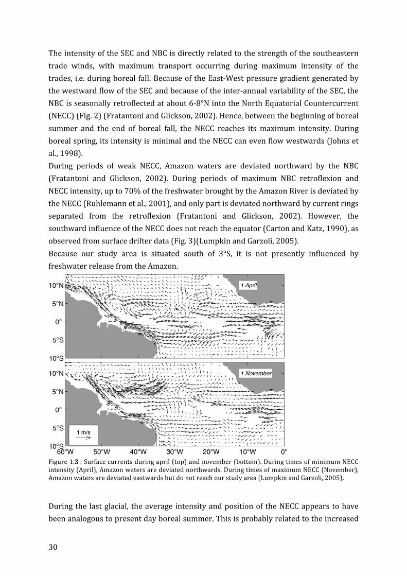
30

The intensity of the SEC and NBC is directly related to the strength of the southeastern

trade winds, with maximum transport occurring during maximum intensity of the

trades, i.e. during boreal fall. Because of the East‐West pressure gradient generated by

the westward flow of the SEC and because of the inter‐annual variability of the SEC, the

NBC is seasonally retroflected at about 6‐8°N into the North Equatorial Countercurrent

(NECC) (Fig. 2) (Fratantoni and Glickson, 2002). Hence, between the beginning of boreal

summer and the end of boreal fall, the NECC reaches its maximum intensity. During

boreal spring, its intensity is minimal and the NECC can even flow westwards (Johns et

al., 1998).

During periods of weak NECC, Amazon waters are deviated northward by the NBC

(Fratantoni and Glickson, 2002). During periods of maximum NBC retroflexion and

NECC intensity, up to 70% of the freshwater brought by the Amazon River is deviated by

the NECC (Ruhlemann et al., 2001), and only part is deviated northward by current rings

separated from the retroflexion (Fratantoni and Glickson, 2002). However, the

southward influence of the NECC does not reach the equator (Carton and Katz, 1990), as

observed from surface drifter data (Fig. 3)(Lumpkin and Garzoli, 2005).

Because our study area is situated south of 3°S, it is not presently influenced by

freshwater release from the Amazon.

Figure 1.3 : Surface currents during april (top) and november (bottom). During times of minimum NECC

intensity (April), Amazon waters are deviated northwards. During times of maximum NECC (November),

Amazon waters are deviated eastwards but do not reach our study area (Lumpkin and Garzoli, 2005).

During the last glacial, the average intensity and position of the NECC appears to have

been analogous to present day boreal summer. This is probably related to the increased

31

thermal gradient between high and low latitudes that induced intensified trade winds,

and enhanced retroflexion of the NBC (Ruhlemann et al., 2001; Wilson et al., 2011). We

conclude that, during both Holocene and the last glacial, freshwater delivered by the

Amazon did not affect the study area, so that the δ18O, 14C and dissolved Pa/Th of

surface waters were undisturbed.

Sediment delivered from the Amazon River and transported to our study area could also

lead to misinterpretation of the Ti/Ca and sedimentary Pa/Th ratio of our sediment

cores. At present, sediment from the Amazon are trapped on the continental margin and

deflected northward by the NBC (Wilson et al., 2011). During glacial times, sea level fell

below the shelf break and most of the sediment delivered by the Amazon River was

deposited on the Amazon fan, i.e. north of the equator (Flood et al., 1995), whereas some

sediment was transported by surface waters along the NECC, affecting for instance the

Ceara rise (Ruhlemann et al., 2001).

We conclude that the sediments reaching our study area are not brought by the Amazon

River but rather by local rivers and in situ carbonate production. Proxies recorded in the

sediment core from my study area can therefore be interpreted without further

complication.

1.3.2. Study area and stratigraphy of the cores

I studied sediment cores that were recovered from the Brazilian margin during R/V

Marion Dufresne cruise MD 173/RETRO3: cores MD09‐3251/52, MD09‐3256Q and

MD09‐3257 (in red in Fig. 4, Table 1). These sediment cores are located at various

depths (~700, ~2300 and ~3500 m) and can therefore record the vertical structure of

the water masses constituting the AMOC. At present, the shallowest core is influenced by

AAIW, the intermediate and deep cores by upper and lower NADW respectively (Fig. 5).

A few marine sediment cores recovered from the North Eastern Brazilian margin during

the R/V Meteor cruise M34/4 and Victor Hensen cruise JOPSII‐6 have been previously

studied (Arz et al., 1999; Jaeschke et al., 2007), some of which are close to RETRO3 cores

(in green in Fig. 4, Table 1).

32

Figure 1.4 : Map of the North Eastern Brazilian margin. Names of RETRO3 cores are written in red and

names of M34/4 cores in green.

Table 1.1 : Name, position and depth of the cores displayed in Figure 1 and discussed in the text. Gravity

cores are indicated in RETRO3 cores by the letter “Q”. RETRO3 cores are otherwise piston cores.

Cruise Name Coordinates Depth (m)

RETRO3 MDO9‐3251Q/3252 04°37.29’S 36°38.69’W 725

RETRO3 MDO9‐3257 04°14.69’S 36°21.18’W 2344

RETRO3 MDO9‐3256Q 03°32.81’S 35°23.11’W 3537

M34/4 GeoB3911 04°36.8’S 36°38.2’W 828

M34/4 GeoB3910 04°14.7’S 36°20.7’W 2362

JOPSII‐6 GeoB3129 04°36.8’S 36°38.2’W 830

MD09-3256Q

MD09-3257

MD09-3251/3252GeoB3911

GeoB3910

Shallow cores

Intermediate cores

Deep core

GeoB3129

33

Figure 1.5 : Phosphate section of the Atlantic Ocean showing the sites of the cores listed in Table 1. White

arrows indicate the approximate flow directions of the Antarctic Intermediate Water (AAIW), Antarctic

Bottom Water (AABW) and North Atlantic Deep Water (NADW).

In this section, I present the stratigraphy work that I have done on the marine

sediment cores in order to choose intervals of interest for the study of last glacial fast

climate variability. X‐Ray fluorescence data on RETRO3 sediment cores were measured

at the Bjerknes Centre for Climate Research (Bergen) and Marum (Bremen). For the

RETRO3 cores, I picked and prepared all planktic foraminifera G. ruber white and

analyzed most of their δ18O on Finnigan Δ+ mass spectrometer. Samples I did not

analyze were measured on an Elementar Isoprime mass spectrometer. I also picked

foraminifera G. ruber white for 14C analyses. Note that 14C dates are not used to build the

age models in this section, but to identify potential turbidites. Precise chronology of the

cores is discussed in chapters 3 and 4.

The Ti/Ca record of sediment cores recovered from the Brazilian margin displays

several peaks during the last 50 ka (Arz et al., 1999, 1998; Jaeschke et al., 2007). These

peaks are associated with periods of increased precipitation on the Brazilian hinterland

that caused increased terrigenous input to the margin and therefore increased

proportion of titanium bearing material with respect to carbonates in marine sediment

cores.

Core GeoB3910 has been extensively studied and its age model is based on 20 14C dates.

Its Ti/Ca record exhibits marked Ti/Ca peaks associated with Heinrich Stadials 1‐5 (Fig.

6) (Jaeschke et al., 2007). As terrigenous peaks are observed in sediment cores of the

entire area, sediment cores from this region can be correlated to the well‐dated

GeoB3910 core.

MD09%3257*

GeoB3910*

MD09%3256Q*

NADW*

AAIW*

AABW*

MD09%3251Q/3252*

GeoB3911*

GeoB3129*

34

Figure 1.6 : Ti/Ca record of core GeoB3910. Each Ti/Ca peak is associated with one Heinrich Stadial (HS1‐

5).

Because core MD09‐3257 was recovered from the same depth and position as

core GeoB3910, Ti/Ca peaks of both cores are quasi identical. When plotted on the

GeoB3910 depth scale, both Ti/Ca records overlap almost perfectly (Fig. 7). δ18O

measurements confirm the good correspondence between the cores, but also highlight

two major differences revealed by δ18O peaks in core MD09‐3257 (Fig. 7). During HS2,

these δ18O peaks are associated with sharp drops in Ti/Ca, but with no significant

change in the Ti/Ca record after HS2. Sand layers occur at the depths of the δ18O peaks

and 14C dating reveals an age inversion within HS2 (Fig. 8). We conclude that δ18O peaks

are associated to turbidite layers, one of which occurs during HS2, therefore preventing

any measurement within this time interval at intermediate depth.

35

Figure 1.7 : (a) δ18O and (b) Ti/Ca signals of intermediate depth cores on the GeoB3910 depth scale.

Figure 1.8 : (a) Ti/Ca and (b) 14C dates (Marine13, (Reimer et al., 2013)) in core MD09‐3257

!2#

!1.5#

!1#

!0.5#

0#

0.5#

1#

1.5#

2#0#

0.5#

1#

1.5#

2#

2.5#

3#

0# 0.5# 1# 1.5# 2# 2.5# 3# 3.5# 4# 4.5#

δ18O%G.%ruber%(white)%

Ti/Ca%

Depth%GeoB3910%(m)%

GeoB3910#

MD09!3257#

(a)#

(b)#

Turbidites#

0"

0.2"

0.4"

0.6"

0.8"

1"

1.2"

1.4"

0"

5"

10"

15"

20"

25"

30"

35"

0" 50" 100" 150" 200" 250" 300" 350" 400" 450"

Ti/Ca"

Age"(ka)"

Depth"(m)"

(a)"

(b)"

MD09%3257*

1" 1.5" 2" 2.5" 3" 3.5" 4" 4.5"0.5"0"

36

The large distance of core MD09‐3256Q from the coast lowers considerably the

terrigenous input to the site, therefore smoothing the Ti/Ca signal in the core. Ti/Ca

peaks are therefore less sharp in core MD09‐3256Q than in intermediate depth cores,

hence complicating the recognition of fast climatic events. An approximate correlation of

core MD09‐3256Q to core GeoB3910 is shown in Fig. 9. A few differences in δ18O are

observed between the two cores. The large deviation of ~0.5 ‰ at the beginning of core

GeoB3910 δ18O record is likely related to the absence of tie points between cores

GeoB3910 and MD09‐3256Q below the depth of HS1. Other small deviations can be

observed and could be explained by the difference in temperature and salinity between

the cores sites (0.2°C and 0.15 psu at present at 30 m depth, Fig. 10), which directly

affects the δ18O of planktic foraminifera. The δ18O peak and Ti/Ca through occurring at

1.64 m (GeoB3910 depth scale) in core MD09‐3256Q is likely related to a large turbidite.

As no sand layers occurs in the core therefore preventing us from visually delimitating

the extent of the turbidite, we used 14C dates instead. As seen in Fig. 11, an age inversion

occurs in the 14C dates measured between 0.66 and 0.88 m (limits not included). We

conclude that the core section delimited by these depths is affected by a turbidite. The

Ti/Ca peak first attributed to HS2 lies within this interval. However, 14C dates indicate

that HS2 is actually situated deeper in the core, and that it is not affected by any

turbidite (Fig. 11). Hence, all fast climatic events of the period between 20‐50 ka are

recorded in core MD09‐3256Q.

37

Figure 1.9 : (a) δ18O and (b) Ti/Ca signals of intermediate (GeoB3910) and deep (MD09‐3256Q) cores on

the GeoB3910 depth scale. Note that correlation of HS2 between core MD09‐3256Q and core GeoB3910

revealed to be incorrect, as inferred from 14C dating.

Figure 1.10 : Present day temperature and salinity at 30 m depth on the Brazilian margin (WOA09).

Deep core

Intermediate

cores

Shallow

cores

Deep core

Intermediate

cores

Shallow

cores

38

Figure 1.11 : (a) Ti/Ca and (b) 14C dates (Marine13, (Reimer et al., 2013)) in core MD09‐3256Q

Core GeoB3911 and neighboring core GeoB3129 are 14C dated by 16 14C dates and show

no apparent hiatus (Arz et al., 1999). They were therefore used for comparison with

RETRO3 shallow sediment cores, which were recovered from their vicinity. Core MD09‐

3251Q is 8.72 m long and is extended by core MD09‐3252 (25.55 m long) (Fig. 12).

Comparison of cores GeoB3911 and MD09‐3251Q/3252 reveals a good correlation from

the core top to the Ti/Ca peak associated with HS1, where the record of core GeoB3911

ends. In core MD09‐3252, the Ti/Ca peak attributed to HS2 exhibits a discontinuity. At

the same depth, the δ18O of G. ruber white jumps towards much lighter values. In other

sediment cores of the region, these light δ18O values are only achieved during MIS5.

MIS3 and MIS4 are thus likely not recorded in core MD09‐3252 and were probably lost

because of a turbidite, as evidenced by the occurrence of a sand layer at the depth of the

abrupt δ18O and Ti/Ca decreases.

0"

0.02"

0.04"

0.06"

0.08"

0.1"

0.12"

0.14"

Age"(ka)"

Ti/Ca"

Depth"(m)"

(a)"

(b)"

MD09%3256Q+

0"

5"

10"

15"

20"

25"

30"

0" 50" 100" 150" 200"

HS2"

0.66" 0.88"0.5"0" 1" 1.5" 2"

39

Figure 1.12 : (a) δ18O and (b) Ti/Ca signals in shallow sediment cores.

We conclude that fast climatic events of the past 20‐50 ka are recorded in the

intermediate and deep sediment cores, but not in the shallow sediment core. I therefore

modified my initial objectives and decided to study HS2 and HS4 on the intermediate

and deep cores. I chose HS2 and HS4 as different northern hemisphere ice sheet

volumes characterize these stadials (Lambeck and Chappell, 2001). It is indeed

interesting to assess the effect of different ice sheet volumes on the configuration and

flow rate of the water masses constituting the AMOC. Even though HS2 is affected by a

turbidite on the intermediate core, it can still be studied at the onset and end of the

event.

41

Chapter 2: Methodology

In my thesis, I dedicated a considerable amount of time implementing and optimizing

the method for the analysis of sedimentary Pa/Th (Yu et al., 1996) at the LSCE. The focus

of this chapter is to detail this method. I measured the protactinium, thorium and

uranium isotopic concentrations necessary for the calculation of the Pa/Th ratio by

isotope‐dilution on a multi‐collector inductively‐coupled plasma mass‐spectrometer

(MC‐ICP‐MS). The principle of isotopic dilution (Vogl and Pritzkow, 2010) is to add a

known quantity of spike (non‐natural isotope in our case) to a sediment sample of

unknown isotopic concentration, and to measure the ratio of both isotopes by mass‐

spectrometry to determine the isotopic concentration of the sediment. Isotopes in the

spike and in the sediment must be of the same element. Measuring protactinium by

isotope‐dilution is complicated by the absence of non‐natural long‐lived protactinium

isotopes. 233Pa is the only non‐natural isotope with a half‐life long enough (26.967 days,

(Audi et al., 2003)) to be used for analysis of 231Pa concentration. However, this half‐life

is short and it is therefore necessary to produce the 233Pa spike a short time before

starting the procedure required for 231Pa concentration measurements. Producing a

233Pa spike can be done either by neutron activation of thorium (Anderson and Fleer,

1982) or by milking of a 237Np solution (Regelous et al., 2004). 237Np indeed decays into

233Pa with a half‐life of 2.14 My (Audi et al., 2003), and secular equilibrium (Np/Pa

activity ratio of 1, maximum concentration of 233Pa) is reached after ~6 months (~6

233Pa half‐lives). Hence, every 6 months, a quantity of 233Pa with the activity of the 237Np

solution can be separated from the 237Np solution and used to spike sediment samples.

This method therefore offers the advantage of providing an unlimited source of 233Pa.

Because the affinity of protactinium for opal is very high (Chase et al., 2002) (see

Chapter 1), I measured the weight percentage of opal (%Opal) in some sediment

samples to investigate whether opal could be a cause of Pa/Th variability in the

sediment cores I studied. Hence, in the first section of this chapter and before discussing

the Pa/Th method, I present the method that I implemented at the LSCE for the

determination of biogenic silica.

In a second section, I present the procedure I used to produce a 233Pa spike by milking of

a 237Np solution. I describe how I calibrated the spikes, i.e. how I measured the 233Pa,

236U and 229Th concentrations, used for the measurement of the Pa/Th ratio,

In a third section, I focus on how I analyzed and corrected the isotopic ratios of interest

by mass‐spectrometry. I also present the equations I used to calculate the sedimentary

Pa/Th ratio.

42

The fourth and final section is the core of this chapter. It is an intercomparison study

(Burckel et al., 2014 c, in prep.) that presents the protocol for sedimentary Pa/Th

analysis that I used and results on various sample types. This study provides an

assessment of the accuracy of the Pa/Th measurements done during my thesis, as well

as an idea of the Pa/Th variability than can be expected when comparing sediment

samples measured in different laboratories.

2.1 Opal measurements

I implemented at the LSCE a method to estimate %Opal in marine sediments by wet

alkaline sequential extraction (Demaster, 2013; Mortlock and Froelich, 1989). Silicate

concentrations are estimated by spectrophotometry, using the heteropoly blue method.

Silica is dissolved and mixed with ammonium molybdate, which forms molybdosilicates

under acidic conditions (Galhardo and Masini, 2000). Consequent reduction of Mo(VI) to

Mo(V) results in the formation of molybdenum blue compounds. The concentration of

these compounds depends on the amount of silicate initially available in the solution,

and results in a more or less pronounced blue colorization of the solution. Silicon

concentration is therefore determined by spectrophotometry, by comparing absorption

intensities of samples to an array of standards of known Si concentration.

2.1.1 Method

Sediment samples were dried and crushed to powder using an agate mortar and pestle.

Sediment was crushed lightly in order to avoid incorporating silica from the mortar and

pestle. ~0.1 g of sediment powder was weighed and transferred to 50 ml centrifuge

tubes. A pretreatment of the sediment is done by addition of 5 ml 10 % H2O2 and 5 ml

1N HCl in order to remove organic matter and carbonates. Tubes were then sonified for

a few minutes and left for 30 minutes. 20 ml MilliQ water was then added to each tube

that were centrifuged, the supernatant decanted to waste. Centrifuge tubes were then

opened and left to dry at 50°C in an oven.

Exactly 40 ml of Na2CO3 (2M) was then added to each tube in order to dissolve biogenic

silica. Sediment was suspended by agitation and centrifuge tubes were placed in a

shaking bath at 85°C. After 2, 3 and 5 hours (Demaster, 2013), centrifuge tubes were

taken out of the bath, centrifuged for a few minutes and cooled in water at ambient

temperature for 5 minutes. 125 µl of each sample are pipetted and transferred to new

centrifuge tubes containing 17.5 ml of molybdate solution (Mortlock and Froelich,

1989), and the centrifuge tubes containing the sediment are closed and put back in the

shaking bath. As this procedure is done at three different times, each sediment sample is

43

associated to three molybdate solutions reacting with the Si extracted after 2, 3 and 5

hours. Centrifuge tubes containing the molybdate solution and the sample aliquot are

mixed by swirling to allow Si to react and complex as molybdosilicates. After exactly 20

minutes, 7.5 ml of reducing solution (Mortlock and Froelich, 1989) is added to each tube

containing the molybdate solution, which is mixed by swirling. Solutions are ready to be

measured the day after, when all molybdosilicates are reduced to molybdenum blue

compounds.

2.1.2 Calculation

Absorptions are measured for each molybdate solution on a spectrophotometer peaked

at 816 nm. Absorptions are then compared to the absorbance‐weight(Si) relationship of

different standards of known Si concentration, to deduce the mass of Si in each

molybdate solution (Fig. 1, Table 1). Si masses are divided by the sediment mass to

calculate %Si in the sediment. Note that his is done for the three molybdate solutions

measured after 2, 3 and 5 hours. The Silicon standard used for calibration of the

absorbance‐weight(Si) relationship is a Silicon AAS standard solution Specpure 500ml

(1000 mg.l‐1).

For each sediment samples, three solutions are measured and their silicon

concentrations inform us about the evolution of Si leaching through time (at 2, 3 and 5

hours). This method is termed “sequential extraction” (Demaster, 2013) and aims at

differentiating the Si extracted by biogenic silica dissolution from alumino‐silicate

leaching. Indeed, while biogenic silica is quickly dissolved (Demaster, 2013), alumino‐

silicates are assumed to continuously leach Si at the same rate through time. Hence, by

measuring the silicate concentration of the extracting solution at different times, we can

estimate the Si concentration resulting from biogenic silica and from alumino‐silicates

(Fig. 2). %Si are multiplied by a factor of 2.139 to calculate %Opal in the sediment

(molar mass SiO2/Si = 2.139 (Muller and Schneider, 1993)).

I compared my results with measurements made at the Institute for Environmental

Physics at the University of Heidelberg (IUP), which routinely analyzes the opal content

of sediment samples using sequential extraction (Muller and Schneider, 1993) (Fig. 3).

Even though I used a different base (Na2CO3 2M) for the dissolution of biogenic silica

than the IUP (NaOH 1 M), our results are coherent. The good efficiency of Na2CO3 could

be related to the relatively young age of our sediment samples (20‐50 ka), as the

resistance of biogenic silica is dependent on the geological period of opal production

(Lyle et al., 2002).

44

Figure 2.1 : Si (mg) as a function of absorbance. Si content of a sample solution is estimated based on its

measured absorbance and on the relation absorbance‐weight(Si) of the standards.

Table 2.1 : Si mass and related absorbance for standards used to form the linear regression in Fig. 1. Si calculated is the estimate of the concentration in the standards based on the linear regression.

Standard Name Absorbance Si (mg) Si (mg) Calculated

Std 0,2mg 0.019 0.2 0.2598447

Std 0,5mg 0.065 0.5 0.4705845

Std 1mg 0.174 1 0.9699462

Std 3mg 0.615 3 2.9902995

Std 6mg 1.274 6 6.0093762

Figure 2.2 : Extraction of Si as a function of time in a sediment sample containing biogenic silica and

alumino‐silicate. After 1‐2h, all biogenic silica is dissolved (Demaster, 2013). Si leaching continues at a

constant rate, which allows finding the initial %Si biogenic in the sample from the intercept.

45

Figure 2.3 : %Opal in two samples measured both at the IUP (blue diamonds) and LSCE (red squares).

2.1.3 Uncertainties

The main uncertainty on the silica concentration of sediment samples is probably

related to the difficulty of disaggregating sediment during alkaline extraction. Sediment

samples from the studied sediment cores are indeed mainly consisted of clays. After the

drying step following the pre‐treatment with H2O2 and HCl, sediment already formed

aggregates although heating was stopped before complete evaporation. Centrifuging

sediment samples also probably caused sediment aggregation, but this step appears

necessary to avoid pipetting silica that would both cause a material loss in the sample

being opal digested, and a high silica gain in the aliquot being analyzed with the

molybdate blue. A pair of full chemistry replicates was measured: one sediment sample

formed a thin cloud when mixed by swirling, and the other formed sediment aggregates

difficult to dissociate. I therefore used the difference of concentration between the two

replicates (0.99 and 0.49 %SiO2) to assess uncertainty on measurements, which are of

34% at 1 SE. Although this uncertainty is large, it is sufficient to estimate the order of

opal concentration of sediment samples.

One procedural blank was also measured. After 5 hours, the weight of Si in the blank

was of 0.017 mg, less than 3 % of the least concentrated sample. Considering the

uncertainty resulting from sediment aggregation, I considered this negligible.

46

2.2 233Pa, 236U and 229Th spikes

2.2.1 233Pa spike milking from 237Np

The 233Pa spike was produced by milking of a 237Np solution following the protocol of

Guihou et al., 2010 (Guihou et al., 2010b). The method takes advantage of the affinity of

protactinium for hydrated silica in the absence of fluorides (Regelous et al., 2004). I used

two neptunium solutions during this thesis, one of 20 kBq and the other of 12 kBq.

Milking of one neptunium solution resulted in ~10‐20 pg of 233Pa, depending on the

activity of the neptunium solution used. These quantities of 233Pa allow the

measurement of 30‐40 sediment samples. After each milking, the neptunium solution

was left to regenerate for 6 months. Here I briefly describe the method of 237Np‐233Pa

separation I used for the production of 233Pa spikes.

A disposable column is filled with 5 ml of hydrated silica gel (63‐200 µm). The gel is

rinsed several times with 8N HNO3 and H2O, and conditioned with 5 ml 8N HNO3. The

neptunium mother solution is evaporated several times to a drop with 8N HNO3 in order

to ensure the absence of hydrofluoric acid in the solution, which could cause Pa losses.

The mother solution is then added to the column in 2 ml 8N HNO3. 23 ml of 8N HNO3 is

then added to the column, by 0.5 ml step for the first 3 ml then by 5 ml steps. Decreasing

the volumes of acids added at each step results in better separation efficiencies as

neptunium immediately enters the gel and is not suspended on the column walls. Once

the neptunium fraction is eluted, the protactinium fraction is extracted with 40‐50 ml

8N HNO3 + 0.13N HF. 233Pa emits gamma rays and its extraction can be monitored using

a COMO170 mobile contamination monitor. We consider that no significant amount of

Pa is left on the column when the gamma counts monitored on the column fall close to

the background level, and when addition of 8N HNO3 + 0.13N HF has no more effect on

the gamma counting, i.e. when no more Pa is eluted. The column is then discarded to a

special radioactive waste container. The 237Np‐233Pa separation is repeated twice to

avoid Np loss in the 233Pa spike which could result in production of 233Pa after the Pa‐Np

separation step. The quality of the 237Np‐233Pa separation was monitored for each spike

by mass‐spectrometry and the 237Np/(233U + 233Pa) ratio always fell below 1.

2.2.2 233Pa calibration

231Pa concentrations were measured by isotopic dilution, but the 233Pa spike was not

directly calibrated. Instead, measurement of a 233Pa‐spiked 231Pa standard was directly

used to estimate the 231Pa concentration of sediment samples (see section 2.4.1).

Estimating the 233Pa concentration of the spike is indeed problematic, as 233Pa decays

into 233U, and as uranium and protactinium can have different ionization efficiencies

(Regelous et al., 2004). In a regular calibration, a known quantity of 231Pa would be

47

added to the 233Pa spike to estimate its concentration by mass‐spectrometry. However,

because 233U and 233Pa may have different ionization efficiencies, the 231Pa addition and

231Pa/233Pa measurement must be done before a significant amount of 233Pa decayed

into 233U. Measuring a 231Pa solution of known concentration, spiked with the 233Pa spike

and U‐Pa separated at the same time as sediment samples can circumvent this problem.

The 231Pa/233(Pa + U) ratio of sediment samples (R(Smp)) and of the 233Pa spiked

231Pa standard (R(Std)) are measured during the same mass‐spectrometer session. 231Pa

concentrations of sediment samples can be calculated by the following equation (1):

�� !"#

!"# =

� �� ∗M!"#$% Smp ∗ �!"#�(��)

� �� ∗M!"#$%(Std)

�!"#

(1)

where [231Pa]sed is the 231Pa concentration of the sediment, Mspike(Smp) and Mspike(Std)

the mass of 233Pa spike in the sediment sample and 231Pa standard respectively, Msed

the sediment mass and N231i(Std) the quantity of 231Pa initially in the the standard.

Usually, the problem of 233Pa decay to 233U is solved by measuring the sediment

samples (231Pa/233Pa ratio) immediately after U‐Pa separation, so that all mass 233

consists of 233Pa. A calibration solution is measured either at the same time, using 231Pa

to estimate the 233Pa concentration of the spike (Auro et al., 2012), or 6 months later

(Negre et al., 2009), when all mass 233 consists of 233U, so that the initial 233Pa

concentration of the spike can be estimated by addition of known amounts of natural

uranium. The advantage of using equation (1) for the estimation of 231Pa concentrations

is that the sediment samples can be measured at any time after U‐Pa separation,

providing more flexibility with respect to the analysis on mass‐spectrometer.

In this study, the 231Pa standard is a HU1 solution of known 238U concentration (see

section 2.2.3 for the estimation of the concentration of HU1). Considering a 235U/238U

activity ratio of 0.04604 (Francois, 2007) and that 235U is at secular equilibrium with

231Pa, we know the 231Pa concentration of the solution.

2.2.3 236U and 229Th calibration

A mixed 236U‐229Th spike was used to estimate uranium and thorium isotopic

concentrations of sediment samples. In this study, using a mix of two spikes is only

useful to avoid weighing each spike separately. The 236U spike was calibrated by spiking

and measuring the 236U/238U ratio of a solution of certified Uranium concentration (SCP

SCIENCE, PlasmaCAL, 1000µg/ml Uranium) by mass‐spectrometry on MC‐ICP‐MS

Neptune. The 238U concentration of the PlasmaCAL solution was calculated by correcting

the total uranium from the 235U contribution, which was done by analysis of the

48

238U/235U ratio by mass‐spectrometry (note that the 238U/235U ratio in the PlasmaCAL

solution is different from the natural 238U/235U atomic ratio of 137.88 (Condon et al.,

2010)). The calibrated 236U spike was then used to estimate the 238U concentration of a

HU1 solution. As HU1 is considered to be at secular equilibrium, its 238U concentration

was used to find its 230Th concentration. The 229Th concentration of the spike was

consequently calibrated by spiking the HU1 solution and measuring the 229Th/230Th

ratio by mass‐spectrometry.

2.3 Measurement by massspectrometry and Pa/Th calculation

2.3.1 Measurements by massspectrometry

Protactinium, thorium and uranium isotopic concentrations were measured by isotope

dilution on a MC‐ICP‐MS (Neptune, Thermo Finnigan). I developed the protocol of

analysis at the LSCE together with François Thil. The cup configurations used for mass‐

spectrometry analysis are presented in Table 2 and 3 for Pa‐U and Th respectively.

Different cup configurations were used because of the different spacing of the cups

required for Pa‐U and Th isotopic measurements. One ion counter was dedicated to

233Pa measurements, as the dark noise on the counter strongly increases during Pa

sample analysis. Dark noise increased typically from 10‐20 counts per minutes (cpm) at

the beginning of the analysis to 100‐160 cpm at the end. The increasing dark noise

during the run is corrected by machine blanks that are measured between each sample.

The dark noise increase is related to the short half‐life of 233Pa, which sticks to the ion

counters, activating them upon decay. After a few months, the dark noise of the ion

counter used for 233Pa measurements decreased back to its initial value, as 233Pa decays

to 233U.

Multiple corrections are applied on the raw spectrometer ratios. Here I describe how

each correction is measured (Table 2, 3). Equations applied to the isotopic ratios or

signals for the various corrections are given in Table 4. I also briefly comment each

correction.

49

Table 2.2 : MC‐ICP‐MS cup configuration for the analysis of U and Pa isotopic ratios. “Solution” column: the

type of solution analyzed, “IC4”‐“H3” columns: ion counters and faraday cups used for isotopic analyses,

“Ratio” column: the ratios of interest, “Use” column: how are the isotopic ratios used, “For” column:

elements for which the measured isotopic ratios are useful. AS stands for Abundance sensitivity. Shaded

cells in column C(C)/IC1 indicate which detector was used (ion counter versus faraday cup). Shaded=C(C),

not shaded = IC1. Cup distances in atomic mass units (u) are shown on top. Lx, Hx and C(C) are faraday

cups, ICx are ion counters.

50

Table 2.3 : MC‐ICP‐MS cup configuration for the analysis Th isotopic ratios. “Solution” column: the type of solution analyzed, “IC4”‐“H3” columns: ion counters and faraday cups used for isotopic analyses, “Ratio”

column: the ratios of interest, “Use” column: how are the isotopic ratios used, “For” column: elements for

which the measured isotopic ratios are useful. AS stands for Abundance sensitivity. Shaded cells in column

C(C)/IC1 indicate which detector was used (ion counter versus faraday cup). Shaded=C(C), not shaded =

IC1. Cup distances in atomic mass units (u) are shown on top. Lx, Hx and C(C) are faraday cups, ICx are ion

counters.

Table 2.4 : Calculation and application of corrections to isotopic signals and ratios. “Correction” column:

type of correction, “Calculation” column: calculation of the correction, “Application” column: application of

the correction on isotopic ratios or signals, “Note” column: notes for clarification of the equations. X and Y

are elements. X can be the same element as Y. Cor. stands for corrected. “u” stands for atomic mass unit.

51

Mass bias: mass bias is calculated using an internal uranium standard with a natural

238U/235U atomic ratio of 137.88 (Condon et al., 2010) (Table 2, 3, 4). Isotopic ratios of all

elements (uranium, thorium and protactinium) are mass bias corrected using the

uranium standard.

Yield IC1‐C(C): The yield is the ratio between the signal measured on the central ion

counter (in cps) and the signal measured on faraday cups (in V, converted to cps using a

factor of 62500000) for a same isotope and solution (Table 2, 3). For my measurements,

this ratio was between 0.9 and 1 and I therefore had to correct the ratio of isotopes

measured simultaneously on IC1 and on faraday cups (Table 4).

Yield IC4‐IC5: Ion counters have different yields. This difference is corrected by

measuring the same isotope (231Pa) twice, but switching the ion counter in between.

Only the 231Pa/233Pa ratio requires this correction (Table 2, 4).

Abundance sensitivity: Abundance sensitivity (AS) (Murray et al., 2013) can significantly

affect isotopic signals on masses close to abundant isotopes. The AS depends on the

resolving power of the mass‐spectrometer. This means that the AS effect of 232Th on

231Pa can be calculated by the effect of 238U on mass 237. Because no isotope is present

at mass 237 in the solution, AS can be directly measured with the M237/238U ratio

(Table 2). The estimation of the AS 2 masses apart is more problematic as there could be

236U in the analyzed solution, thus, the measured M236/238U ratio is not a direct

representation of the AS. The AS two masses appart is therefore estimated by

exponential interpolation of the AS signal on masses 235.5 and 236.5 (Table 2). A

retardation lens (RPQ) on IC1 allows to decrease the effect of AS. Because 231Pa is not

measured on IC1 (no RPQ), AS is not measured on IC1 for correcting the contribution of

232Th on the 231Pa signal (Table 2).

Hydrides: Hydrides (X‐H+ where X is an isotope) (Murray et al., 2013) can significantly

affect isotopic signals that are one mass above abundant isotopes. Hydrides formation is

element dependent and more important for thorium than for uranium (by a factor of

~2). Uranium hydrides are corrected by measuring the 239/238U ratio, while thorium

hydrides are corrected with the 233/232Th ratio in a 233U free solution.

Natural isotopes in the spike: Signals are corrected from the presence of 230Th in the

229Th spike. 232Th in the 229Th spike is negligible, as are 234U, 235U and 238U in the 236U

spike. 231Pa in the 233Pa spike is not negligible but is corrected with chemistry blanks.

52

Chemistry blanks: Chemistry blanks are estimated by measuring a mixture of 236U, 233Pa

and 229Th spikes that was processed as a sediment sample. One blank is measured for

each batch of 9 samples. The blank’s natural isotopes on tracer ratios are then removed

from sediment samples ratios.

2.3.2 Pa/Th calculation

The Pa/Th ratio is the ratio of excess protactinium and thorium activities, corrected

from decay to the time of sediment deposition. Excess protactinium (thorium) is

calculated by subtracting from the total protactinium (thorium) the protactinium

(thorium) resulting from authigenic uranium decay and protactinium (thorium)

supported by uranium present in the sediment mineral lattices (lithogenic). We can

write:

� !"#$%&"' = � !"#!!"#$%& + � !"#!!"#$!% + � !"#!$$ (2)

where X is 231Pa or 230Th and (X)measured is the total 231Pa or 230Th, which is measured by

mass spectrometry.

232Th is mainly of lithogenic origin and lithogenic uranium can therefore be calculated

from the lithogenic 238U/232Th ratio (R), assumed to be equal to 0.5 ± 0.1 (Guihou et al.,

2010b). As a consequence, lithogenic protactinium (thorium) can be calculated as it is

assumed to be at secular equilibrium with lithogenic 238U (235U). As 238U consists of

lithogenic and authigenic uranium, knowing lithogenic 238U and total 238U allows the

calculation of authigenic 238U. Assuming a 234U/238U activity ratio of 1.1466 (Robinson et

al., 2004a) in the ocean and a natural 235U/238U activity ratio of 0.04604 (Francois,

2007), we can estimate the protactinium and thorium produced by authigenic 235U and

234U respectively since the time of sediment deposition.

Equations (3, 4) detail the calculation of excess thorium and protactinium, for more

information refer to (Henderson and Anderson, 2003):

�ℎ !"#

!"#!$$ = �ℎ !"#

!"#$%&"' − �ℎ !"!

!"#$%&"' ∗�

!"#

�ℎ !"!

!"#!!"#$%&

−�

!"#

� !"#

!"#$%

∗ � !"#

!"#$%&"' − �ℎ !"!

!"#$%&"' ∗�

!"#

�ℎ !"!

!"#!!"#$%&

∗ 1− �!!!"#∗! (3)

53

�� !"#

!"#!$$ = �� !"#

!"#$%&"' −�

!"#

� !"#

!"#$%"&

∗ �ℎ !"!

!"#$%&"' ∗�

!"#

�ℎ !"!

!"#!!"#$%&

−�

!"#

� !"#

!"#$%"&

∗ � !"#

!!"#$%!& − �ℎ !"!

!"#$%&"' ∗�

!"#

�ℎ !"!

!"#!!"#$%&

∗ 1− �!!!"#∗! (4)

where t is the time since sediment deposition and λ are the decay constants of 231Pa or

230Th.

Excess protactinium and thorium are then corrected from decay since the time of

sediment deposition by the following equation:

� !"#!$$,! = � !"#!$$ ∗ �!!!∗! (5)

where X is 231Pa or 230Th.

Calculation of measurement uncertainties is based on the work of Guihou et al., 2010.

Analytical and systematic errors are propagated through the Pa/Th equations assuming

that all variables are independent and have a Gaussian distribution (Guihou et al.,

2010a).

2.4 Pa/Th sediment results and intercomparison

2.4.1 Methodological recommendations for the analysis of sedimentary Pa/Th.

This article has already been reviewed by all co‐authors, and corrections have been

implemented. Information concerning the method of uncertainties calculation and 231Pa

standard calibration will be added before submission to Analytical Chemistry. The

masses of 233Pa, 236U and 229Th used by the LDEO to spike sediment samples are still

missing in Table 1 but will not change the content of the article.

54

Methodological recommendations for the analysis of sedimentary Pa/Th.

P. Burckel1, G. Henry2, H‐C Ng3, J. Lippold4, S. Pichat5, M. Roy Barman1, F. Thil1, J.

Gherardi1, C. Waelbroeck1, J.F. McManus2, L.F. Robinson3, B. Antz4

1LSCE/IPSL, Laboratoire CNRS‐CEA‐UVSQ, Bât.12, avenue de la Terrasse, F‐91198 Gif

sur Yvette, France

2Lamont‐Doherty Earth Observatory of Columbia University, P.O. Box 1000, Palisades,

NY 10964 USA

School of Earth Sciences, University of Bristol, Wills Memorial Building, Queen's Road,

Clifton BS8 1RJ

4Oeschger Centre for Climate Change Research, Institute of Geological Sciences,

University of Bern, Zähringerstrasse 25, CH‐3012, Bern, Switzerland

5Laboratoire de Géologie de Lyon (LGL‐TPE), Ecole Normale Supérieure de Lyon, 46

allée d'Italie, 69007 Lyon, France

Abstract:

We present recommendations for the measurement of sedimentary U, Th and Pa

isotopes using isotope dilution method. Our study is based on an interlaboratory

comparison of different protocols and massspectrometers. We provide a detailed

comparison of the methods in terms of efficacy, rapidity, and acid volumes used,

which serves as reference for emerging Pa/Th laboratories to develop their

protocols based on available equipment and facility. Concentration results

highlight the necessity of complete homogenization of distributed sediment

samples prior to any intercalibration study, for instance by using a coning and

quartering method. This study also provides and validates a new method of

measurement of 231Pa concentrations, which allows Pa massspectrometer

measurements to be done at any time after UPa separation. Finally, we provide

an estimate of the current interlaboratory Pa/Th variability based on results of

the four participating laboratories.

Introduction

U‐series decay products, such as 230Th, 231Pa, 232Th, 234U, and 238U, can be used for

a wide array of applications in geosciences. For example, deviation of their isotopic

55

ratios from secular equilibrium (activity ratio of 1) allows age determination of

geological events 1,2, quantification of weathering rates 3 and riverine sediments transfer

time 4. In paleoceanography, sedimentary 230Th concentrations can be used to examine

post‐deposition sediment redistribution (focusing and winnowing) 5,6 or variations in

vertical particle flux 7,8, and the sedimentary (231Pa/230Th)xs,0 activity ratio (Pa/Th

hereafter) is used as a proxy for vertical particle flux 9, changes in productivity 10, and

variations in ocean circulation intensity 11‐15.

Sedimentary Pa/Th is usually measured by isotope dilution. The chemical

methods used to purify the radionuclide isotopes of interest in the bulk sediment mostly

follows the early work of Anderson et al 16. These methods usually comprise the

following steps: 1) sediment spiking and digestion, 2) separation of actinides from the

sediment matrix, notably alkali and alkaline earth metals which is often done by

oxyhydroxide precipitation, 3) Pa, Th, and U purification, and 4) measurements by

Inductively‐Coupled Plasma Mass‐Spectrometry (ICP‐MS) 17‐19, that has replaced alpha

and beta counting 11,16 over the years. 233Pa spike decays into 233U (T1/2= 26.967d 20) that

may have different ionization efficiency 17. Spike calibration is therefore done either

when all mass 233 consists of protactinium, i.e. typically within 24h after U‐Pa

separation 17,21, or when all 233Pa is decayed into 233U, i.e. more than 6 months after U‐Pa

separation 22.

The present study provides, in details, some of the main methods available for the

analysis of sedimentary Pa/Th by different mass‐spectrometers. We apply these

methods to various samples and discuss the results. The methods are assessed in terms

of optimal sediment digestion, U‐Th‐Pa separation and purification, and procedural

yields. We also assess the quickest methods, as well as those requiring the least acid

volumes. Based on the results, we provide recommendations for homogenized

distribution of sediment sample prior to inter‐laboratory analysis, and the pros and cons

of each of the methods and mass‐spectrometers. We also present a new method to

measure sedimentary 231Pa concentrations, circumventing the problem of the 233Pa

decay and allowing protactinium samples to be measured at any time after separation of

uranium from the protactinium fraction. Finally, we compare Pa/Th results of the

different laboratories and examine potential inter‐laboratory Pa/Th variability. Four

Pa/Th laboratories participated in this study for the measurements: the Laboratoire des

Sciences du Climat et de l’Environnement (LSCE), the University of Bristol (UB), the

Lamont Doherty Earth Observatory (LDEO) and the Institute for Environmental Physics

at the University of Heidelberg (IUP).

56

Experimental section

Isotopic reference material. Thorium isotopic reference material IRMM‐035 and

uranium isotopic reference material NBS‐SRM‐960 (also called CRM 112‐A) were

analyzed for 230Th/232Th and 234U/238U, respectively, to assess both precision and

accuracy of the isotope‐dilution ICP‐MS measurements.

Solid Samples. Three solid samples were analyzed for their Pa, Th, and U isotopic

concentrations. Geotraces_Sed is a near‐surface siliceous ooze sediment (71% biogenic

silica, 7% CaCO3) recovered during a cruise of the RVIB Nathaniel B. Palmer (NBP9604

Station 3, 61.95°S/170.05°W, 3404 m water depth) 23. This sample was previously

measured as part of the GEOTRACES intercalibration study 23, which makes it valuable

to assess data quality of this study. Margin_Sed is an early Marine Isotope Stage 2

sediment sample, recovered during a cruise of the R/V Marion Dufresne (MD

173/RETRO3, 03.55°S/35.39°W, 3537 m water depth) from the Brazilian margin, which

mainly consists of calcium carbonate and terrigenous material. Sediment ages are given

in Supporting Information. UREM11 is a uranium ore reference material, certified for its

uranium concentration and supplied by the Council for Mineral Technology, South Africa

24. The three samples have very different isotopic composition and span most of the

Atlantic sediment 231Pa and 230Th concentration range (0.2‐1 and 1‐12 dpm.g‐1

respectively 25) and the lower part of the Pacific range (0.1‐6.5 and 1‐190 dpm.g‐1

respectively 26). Therefore they allow a thorough assessment of the presented Pa/Th

methods.

Sample homogeneity. The problem with sediment heterogeneity when measuring

230Th was raised by the GEOTRACES program and might lead to inter‐laboratory

variability 23. The sediment sample from the GEOTRACES intercalibration

(Geotraces_Sed) was therefore split using the coning and quartering method (Fig. S1) in

order to assess the effect of this procedure on sediment heterogeneity. Sediment was

then sent to the laboratories participating in this study. Margin_Sed was hand powdered

with an agate mortar and pestle. The resulting powder was distributed stepwise and

alternatively among the different shipment containers until all containers were full. The

sediment was then sent to the participating laboratories. Sediment distribution was

systematically done with a spatula. Sediment was not poured but deposited in the

containers. These cautions aimed at minimizing the risk of grain size sorting during

distribution. No particular care was taken with respect to sample homogeneity for the

distribution of the UREM11 reference material, as this sample is a solid standard of

small grain size (<75µm) therefore expected to be homogeneous.

57

Safety considerations. All methods require adequate protection equipment for the

various reagents used, such as lab coats, nitrile gloves and safety glasses. Handling

hydrofluoric acid usually requires additional precautions (refer to local regulations).

Acids must be handled and evaporated under a chemical fume hood. Solution containing

perchloric acid must be evaporated in hoods certified for such use. Radioactive tracers

have to be used following the local regulation.

Sample weighing, spiking and digestion. Sediment sample powders and spike are

weighed and mixed, except for UB that adds spikes after sediment digestion. The

approach used by UB necessitates the prevention of any material loss before spike

addition, and in microwave digestion this is achieved by the use of microwavable closed

pressurized vessels.

Sediment mass and spike quantities used by each lab are given in Table 1. They

do not differ significantly except for the much lower amount of 236U spike used by the

LSCE (see Discussion).

Sample digestion methods are detailed in Table 1. They mainly differ by the use

of microwave or hotplate.

Oxyhydroxide precipitation. After the digestion step, samples are evaporated to semi‐

solid gel, which is consequently dissolved in HCl (UB, LDEO) or HNO3 (LSCE, IUP) and

heated to clear solutions at 150‐180°C (LSCE, UB). At this point, sample‐spike

equilibration should have been reached 27, thus any subsequent material loss would not

impact the final concentration results. However, the methods used for purification and

separation of radionuclides influence the yield and purity of each element, which

ultimately impact the precision and accuracy of the mass‐spectrometer measurements

as well as the magnitude of the applied corrections.

Three laboratories (LSCE, UB, LDEO) use the classical step of separation of the

radionuclides from the alkali and alkaline earth metals by oxyhydroxide precipitation 16.

Briefly, digested sample solutions are transferred to centrifuge tubes and NH4OH is

added until the formation of Fe‐Al precipitates at around pH = 8. The samples are then

centrifuged, and the supernatant decanted to waste. Precipitates are washed several

times. The number and type of washes is the main difference between the three

laboratories. After the first co‐precipitation, precipitates are washed with 18.2 MΩ

water and a few drops of ammonia (LSCE, UB: 20ml H2O LDEO: 5ml). The washing step

is achieved by agitation of the centrifuge tube to re‐suspend the precipitate. Tubes are

then centrifuged and the supernatant decanted to waste. The LDEO and UB group then

dissolve the precipitate in 2 ml and 20 ml HCl 9N, respectively, for column separation.

58

The LSCE group dissolves the precipitate in 20 ml HNO3 2N, before oxyhydroxide co‐

precipitation with ammonia. Tubes are then centrifuged and the supernatant decanted

to waste. The precipitate water washing/acid dissolving process is repeated once.

Precipitate is then washed one last time with MilliQ water and a few drops of ammonia,

before samples are centrifuged and the supernatant decanted to waste. The precipitate

is then dissolved in 2 ml HNO3 8N for column separation.

The large number of water washing/acid dissolving steps achieved by the LSCE is

meant to better separate U, Pa, and Th from alkali and alkali earth metals. However, the

separation efficiency was not verified, and it could be that these time‐consuming steps

reduce the chemistry yield without major improvement of the separation.

IUP skips the oxyhydroxide precipitation step as this process is time consuming.

This could however lead to poorer elemental separation and purification by anion‐

exchange chromatography because of a higher matrix load, which could both diminish

the ionization efficiency and increase the interferences during mass‐spectrometry

measurements. These side effects thus need to be monitored and corrected for.

Pa, Th, and U separation and purification. The four labs use slightly different anion‐

exchange chromatography separation and purification step (Fig. 1). The method used by

the LSCE is derived from Guihou et al 28. Whole chemistry yields and elemental

separation efficiencies are given in Table 2.

Analysis by massspectrometry. Precision and accuracy of the analyses by mass‐

spectrometry depend on many variables, some inherent to the type of mass‐

spectrometer and introduction system (Table 3) and some due to the previous

chemistry steps (Table 2). We compared three types of ICP‐MS in this study: multi‐

collector (MC) (LSCE and UB; Thermo‐Fisher Finnigan Neptune), sector‐field single‐

collector (SF) (LDEO; Finnigan Element XR), quadrupole single‐collector (Q) (IUP;

Thermo Scientific iCAP Qs).

231Pa concentration measurements. As 233Pa decays rapidly to 233 U (T1/2= 26.967d),

which possibly has a different ionization efficiency 17, the 231Pa/233Pa ratio is usually

measured within 24h 17 after U‐Pa separation. Different methods to estimate sediment

231Pa concentrations were used by the laboratories participating in this study. UB and

LDEO measure the 231Pa/233Pa ratio 1 and 3 days after Pa‐U separation respectively, i.e.

before the decay of a significant fraction of the 233Pa spike. Moreover, the LDEO group

considers that the ionization difference between Pa and U is negligible on their SF‐ICP‐

59

MS, based on the results obtained by Choi et al 19 on the same type of instrument. This

allows them to estimate the concentration of the 233Pa spike, which in turn is used to

estimate the 231Pa concentration of sediment samples. However, these methods require

mass‐spectrometer measurements to be done immediately after column

chromatography.

Here we present the new method of measurement of 231Pa concentrations developed by

the LSCE and IUP. It presents the advantage of removing the time constraints on mass‐

spectrometer measurements linked to the short 233Pa half‐life.

233Pa spike is added both to sediment samples and to a 231Pa solution of known

concentration. After sediment digestion, the Pa fractions of the sediment samples and of

the spiked 231Pa standard are separated from U at the same time by column

chromatography. The 231Pa/233(Pa + U) fractions can be measured at any time after

separation, as long as the samples and spiked 231Pa standard are measured during the

same mass‐spectrometer run (within ~24h 17). Here we briefly present the

mathematical validity of this method of measurement of 231Pa concentrations, for more

details refer to SI.

Consider a 231Pa standard of known concentration spiked with a 233Pa solution of

unknown concentration, and a digested sediment sample spiked with the same 233Pa

solution. The Pa fraction of both solutions was purified from U at the same time by

column chromatography. When measured on mass‐spectrometer, the spiked 231Pa

standard contains N231(Std) and N233(Std) atoms of 231Pa and 233(Pa + U) respectively.

The sediment sample contains N231(Smp) and N233(Smp) atoms of 231Pa and 233(Pa + U)

respectively. The 231Pa/233(Pa + U) ratio R measured on mass‐spectrometer for any of

the solutions depends on α, the U/Pa ionization efficiency ratio, and on t2, the time since

column elution, which dictates the proportion of Pa and U in the solution:

� =�!"#

�!"" ∗ �(�2,�)=

�!"#�

�!""� ∗ �(�1, �2,�)=

�!"#�

�!"#$% ∗ [ �� !"" ]! ∗ �(�1, �2,�)

(1)

N231i and N233i are the number of atoms of 231Pa and 233Pa respectively present before

digestion for sediment samples and before column chromatography for spiked 231Pa

standards (i.e. initial concentrations). A depends on t2 and α, B depends on t1, the time

between spike creation and column elution as well as on t2 and α, [233Pa]i is the

unknown initial concentration of the 233Pa spike, MSpike is the known mass of spike

added to the sample. α equals 1 if there is no ionization difference.

For a spiked 231Pa standard (Std) we can write:

[ �� !"" ]! ∗ B t1, t2,α =

�231� ��

MSpike Std ∗ � ��(2)

60

Equation (2) can be inserted in equation (1) for a sediment sample (Smp) in order to get

rid of the unknown initial spike concentration and of B(t1,t2,α), as this term is the same

for sediment samples and spiked 231Pa standards which are U‐Pa separated and

measured on mass‐spectrometer at the same time.

We obtain:

�� !"#

!"# =

� �� ∗M!"#$% Smp ∗ �!"#�(��)

� �� ∗M!"#$%(Std)

�!"#

(3)

where [231Pa]sed is the concentration of the sediment sample and Msed is the sample

mass. R(Smp) and R(Std) are measured by mass‐spectrometry, N231i(Std), Msed,

Mspike(Smp) and Mspike(Std) are known or weighed.

Results and discussion

Isotopic ratio accuracy and precision. As a first step, thorium IRMM‐035 and uranium

NBS‐SRM‐960 isotopic reference materials were measured to evaluate mass‐

spectrometer accuracy and precision. Results for each laboratory are shown in Fig. 2,

along with certified ratios.

MC‐ICP‐MS (LSCE, UB) give accurate measurements (see Table S1), within uncertainties

for both isotopic ratios and their precision are better (ca. 8 times better) than other ICP‐

MS types (Fig. 2). Single collector ICP‐MS (LDEO, IUP) display an offset from thorium

and uranium certified isotopic ratios of up to several percent and can have variable

results. This offset may be due to the low concentration of the standard solutions (0.01‐

0.02 dpm.g‐1) as shown by the results in the next section. Note also that the series of

measurements made by the IUP group in this study is one of the first made by their Q‐

ICP mass‐spectrometer. Accordingly, performance may not be comparable to a mass‐

spectrometer routinely used for several months.

Pa, Th and U isotopic concentrations on solid samples. Protactinium, thorium and

uranium isotopes concentrations of solid samples (sediments and uranium ore

UREM11) measured by isotope‐dilution in this study are shown in Table S2 and Figures

S2‐S6. Figure 3 and 4 summarize these results by showing deviations (in %) of the

isotopic concentrations of each laboratory from the inter‐laboratory mean.

61

Protactinium, thorium and uranium isotopes concentrations of sediments and

uranium ore UREM11 measured by the 4 laboratories generally agree within 2 sigma

uncertainties (Fig. 3, 4, see also Table S2 and Fig. S2‐S6). The only outliers are the 230Th

and the 234U concentrations measured on Margin_Sed by the LDEO. Moreover, no

laboratory displays a systematic positive or negative deviation from the inter‐laboratory

mean on U‐Th measurements. Systematic biases such as different spike calibrations and

digestion efficiencies are therefore not the main factors leading to inter‐laboratory

concentration differences for U and Th. A systematic Pa concentration bias could be the

reason for the differences between LSCE and UB results. It is unlikely that this difference

results from incomplete organic matter degradation 22, as both labs use perchloric acid.

Systematic concentration differences could be related to issues in the estimation of the

concentration of the 231Pa standard used for spike calibration or to an effect of the two

methods of measurement of 231Pa concentrations used by the LSCE and UB groups. The

validity of the new 231Pa concentration measurement method used by the LSCE and IUP

groups is assessed later in this study. The UREM11 sample displays the most consistent

inter‐laboratory concentration results (Fig. 3, 4). This is probably due to its high

concentration and homogeneity. This result tends to confirm that isotopic ratio offset

and variability measured on single collector ICP‐MS was due to the low concentrations

of the standards. Our results on Geotraces_Sed are also consistent with the GEOTRACES

intercalibration, confirming the validity of the presented methods (Table 4).

Small quantities of 236U spike are used for measurement on the LSCE MC‐ICP‐MS

(Table 1). The mass‐spectrometer is also used for U‐Th dating, for which precision of

uranium measurement is critical. The LSCE group therefore had to find a trade‐off to

allow multiple utilization of the instrument. Using low concentrations of 236U for Pa/Th

measurements reduces machine blank levels and carry‐over, which increase the

precision for dating of low concentration uranium samples. As a consequence, the 236U

had to be measured on an ion counter for Pa/Th, which could decrease the precision

compared to measurements of higher spike quantities on faraday cup. However,

precision on uranium concentration measurements is quite similar between the MC‐ICP‐

MS users (LSCE and UB), despite the different mass of 236U used. Low 236U spike

quantities can therefore be used to precisely measure the uranium concentration of

sediment samples.

Comparison of the digestion methods: microwaveassisted versus hotplate. Both

microwave and hotplate digestion were used by the UB group in order to compare

digestion efficiencies. Results are shown in Fig. 5. Almost all pairs of measurements

(hotplate‐microwave) are similar within error bars. Moreover, none of the two digestion

methods yields systematically lower or higher isotopic concentrations. Hence we

62

conclude that microwave and hotplate digestion have similar efficiencies. Microwave

digestion is therefore not necessarily the most efficacious digestion method, unlike

stated in earlier studies 30.

Heterogeneity effects. In the GEOTRACES intercalibration, concentration

measurements on Geotraces_Sed showed that the inter‐laboratory variability of 230Th

measurements was similar to the intra‐laboratory variability of some laboratories

(range of 5‐6 dpm.g‐1) 23. For this reason, the authors concluded that the sediment that

was distributed to the participating laboratories was heterogeneous. Prior to

distributing the Geotraces_Sed sample for this study, we homogenized the sediment

using the coning and quartering method. The inter‐laboratory 230Th concentrations we

obtain on Geotraces_Sed shows much less variability than in the GEOTRACES

intercalibration (2.3%, 2 sigma, range of 5‐5.6 dpm.g‐1). This result indicates that the

original GEOTRACES intercalibration indeed measured heterogeneous material.

Grinding and mixing of sediment before a thorium inter‐calibration study therefore

appears insufficient, and a more intense sediment homogenization method needs to be

used for inter‐comparisons.

Evaluation of the new method of measurement of 231Pa concentrations. The good

consistency of the Pa measurements indicates that the 2 methods used by the four

laboratories to measure 231Pa concentrations (i.e., Pa measurement immediately after

column separation for the UB and LDEO group and possibly a few weeks after for the

LSCE and IUP groups) have a minor impact on the results. However, in this study, Pa

solutions were analyzed quite quickly after column separation even for the LSCE and

IUP groups (4 and 7 days after column separation respectively). Moreover, there is an

offset between UB and LSCE Pa concentration results, which could be attributed to the

different methods of measurements of 231Pa concentrations or to the estimation of the

concentration of the 231Pa calibration solution.

Hence, to demonstrate the validity of the 231Pa measurement method described

in this paper, protactinium concentrations of pairs of full sediment replicates were

analyzed by the LSCE group at different times between U‐Pa separation and

measurement on ICP‐MS, i.e. with different 233U/233Pa ratios. All first replicates are

measured 6 days after U‐Pa separation, except one which is measured after 10 days

(square on Fig. 6, more details hereafter). Second replicates are measured 13 to 52 days

after U‐Pa separation. If our method of 231Pa measurement is robust, the additional time

left for 233Pa to decay between the measurement of the first and second replicates

should not impact concentration results. We therefore present our results as deviations

63

(%) of the concentration of one replicate from the other, and as a function of the

additional time left for the 233Pa to decay in the second replicate (Fig. 6, Table S3). One of

the presented pair of replicates is not composed of two full sediment replicates but of a

single sample whose Pa fraction was measured at two different times (10 and 52 days,

square on Fig. 6). Although its 233(Pa + U)/231Pa ratio varies by more than 20% (0.629 to

0.494) reflecting the higher ionization efficiency of Pa compared to U, the 231Pa

concentration varies only slightly (1.6%, 0.197 to 0.194 dpm.g‐1), almost within the

statistical uncertainty of the measurements (Table S3). Moreover, we see that full

sediment replicates measured at different times do not display a systematic increase or

decrease of their Pa concentration with time (Fig. 6). This confirms that the method of

measurement of 231Pa concentration presented in this paper can be used even if

uranium and protactinium have different ionization efficiencies. The major advantage of

this method is that it is not time dependent as other methods that necessitate the spike

calibration to be done either immediately after U‐Pa separation 17,21 or more than 6

months later 22. Note however that the spiked 231Pa standard solution and protactinium

blanks need to be measured at the same time as the samples (within 24h, 17) and it is

therefore necessary to produce enough blank and standard solution. Blanks are also

needed because the 231Pa/233(Pa + U) ratio in the blank changes through time and

therefore needs to be measured at the same time as the samples.

Given the consistency of this new 231Pa measurement method, it is more likely that the

Pa concentration differences between the LCSE and UB groups (Fig. 3) result from issues

on the estimation of the concentration of the 231Pa solution used for the calculation of

sedimentary 231Pa concentrations.

Sedimentary Pa/Th calculation and variability. Inter‐laboratory comparison of

particulate and dissolved Pa/Th measurements is one of the ultimate targets of the

GEOTRACES program. In order to have an idea of the current inter‐laboratory Pa/Th

differences, we calculated the Pa/Th values associated to both sediment samples

measured in this study.

The inter‐laboratory mean Pa/Th of the Margin_Sed sample is 0.065 ± 0.008 (13.1% 2

sigma) and the mean of the Geotraces_Sed sample is 0.222 ± 0.016 (7.3% 2 sigma) (Fig.

S7, Table S4). The Pa/Th result from the LDEO is excluded from the calculation of the

mean Pa/Th on the Margin_Sed sample because of its anomalously low 230Th

concentration (Fig. 4). Maximum Pa/Th differences between two labs are 12.2% for the

Margin_Sed sample and 9.1% for the Geotraces_Sed sample. Such differences are

significant and highlight the necessity to continue and intensify intercalibration efforts.

64

Pa/Th differences are however lower between the laboratories using multi collector

mass‐spectrometers, with 5.6% difference on both samples. By intercalibrating spikes

and 231Pa standards, it could be possible to increase the consistency of the

measurements.

Advantages of the presented methods. Table 5 lists the best chemistry methods based

on three main categories: efficacy, rapidity, as well as on the lowest acid volumes used.

The most efficacious digestion is the most complete, and the most efficacious U‐Th‐Pa

separation achieves the highest separation and yield.

All methods are equally efficacious concerning sediment digestion. Given the separation

efficiency and yield in Table 2, the UB group method achieves the most efficacious U‐Th‐

Pa separation. High yields allow more precise measurement of Pa, Th and U

concentrations. The high separation efficiency of the elution by column chromatography

minimizes the corrections applied to the ratios measured on mass‐spectrometer and

therefore maximizes precision.

Using microwave digestion is the quickest method (a few hours, Table 1), as hotplate

requires samples to be heated overnight. Both the UB and IUP methods can therefore be

used. The most rapid column chemistry is achieved by the IUP group by not having a Th

purification step (Fig. 1). However, the higher matrix load resulting from the absence of

separation could result in matrix effects on some mass‐spectrometer, particularly given

that the IUP group skips the oxy‐hydroxide separation 31.

Pa/Th analyses are expensive and require large waste treatment due to the large

amounts of acid used that therefore need to be minimized. The LDEO achieves digestion

with the lowest volume of acids (6 ml/sample) (Table S5). The LSCE method uses the

smallest volume of acids during the column chemistry step (98 ml/sample).

Massspectrometer recommendations. The sensitivity of the Q‐ICP‐MS is lower (6‐40

times) than the LSCE MC‐ICP‐MS, which has a similar introduction system (Table 3).

Moreover, the poor abundance sensitivity of the Q‐ICP‐MS makes precise 231Pa

measurements difficult if 232Th is not separated well enough. Given the method used by

the IUP group, 231Pa abundance sensitivity correction on the sample with the highest

232Th/231Pa ratio (Margin_Sed, 232Th/231Pa = 4.3×106) is 58% of the total 231Pa signal.

This correction is calculated based on the separation efficiency of Th from the Pa

fraction in Table 2, on abundance sensitivity correction in Table 3 and on the

sedimentary 232Th/231Pa atomic ratio. We therefore recommend to use this mass‐

spectrometer with the most efficacious Pa‐Th separation method (UB) only (Table 2),

and to avoid its use for Pa/Th measurements of samples with high 232Th/231Pa atomic

ratios.

65

The UB and LDEO groups use an Aridus desolvating nebulizer system. This greatly

reduces hydrides and increases sensitivity. Tests with the Aridus II performed by the

LSCE group show a 10‐fold decrease in hydrides and 3‐fold increase in sensitivity. Side

effect is the large sample gas (Ar) consumption increased by 10 times. It is known that

such systems impact sensitivity and hydrides, but the Aridus is better than a simple

desolvating membrane plugged after the Apex HF (2‐fold sensitivity increase, 4‐fold

hydrides decrease). The LSCE group did not use the Aridus but an Apex HF system (no

desolvating membrane) for measurements presented in this study.

Conclusions

Many Pa/Th analysis methods exist, each with their own specificities. The four methods

used in this study achieve coherent results. However, progress can be made to improve

inter‐laboratory variability of Pa/Th measurements, which is in this study of 5.6 % at

best. The first step to achieve is to distribute homogeneous sediment samples prior to

intercalibration studies. A coning and quartering method is proven to be adequate for

this purpose. Results could also be made more consistent through the intercalibration of

spikes and calibration solutions. Finally, our new method of measurement of 231Pa

concentrations should facilitate the measurement of sedimentary Pa/Th, by giving more

flexibility with respect to the analysis on mass‐spectrometer that can be done long after

the separation of U from the Pa fraction by column chromatography.

Acknowledgments

Measurements performed at LSCE were funded by the CNRS/INSU LEFE project

ACCENT. This work is a contribution to the RETRO project, a joint European Science

Foundation (ESF)/EUROMARC, funded by Research Council of Norway (RCN), France

(CNRS/INSU), Germany, and the Netherlands. Part of the sedimentary analyzed was

collected on board R/V Marion Dufresne during RETRO Cruise III, supported by ESF

EUROMARC project RETRO, IPEV and ANR project ANR‐09‐BLAN‐0347. We thank the

IPEV team, crew members of R/V Marion Dufresne and all scientists who participated in

RETRO Cruise III. This is LSCE contribution xxxx.

References

(1) Knight, A. W.; Eitrheim, E. S.; Nelson, A. W.; Nelson, S.; Schultz, M. K. Journal of

environmental radioactivity 2014, 134, 66‐74. (2) Martinez‐Aguirre, A.; Alcaraz‐Pelegrina, J. M. Journal of Radioanalytical and Nuclear

Chemistry 2013, 298, 1005‐1016.

(3) Chabaux, F.; Blaes, E.; Stille, P.; Roupert, R. d. C.; Pelt, E.; Dosseto, A.; Ma, L.; Buss, H.

L.; Brantley, S. L. Geochimica Et Cosmochimica Acta 2013, 100, 73‐95.

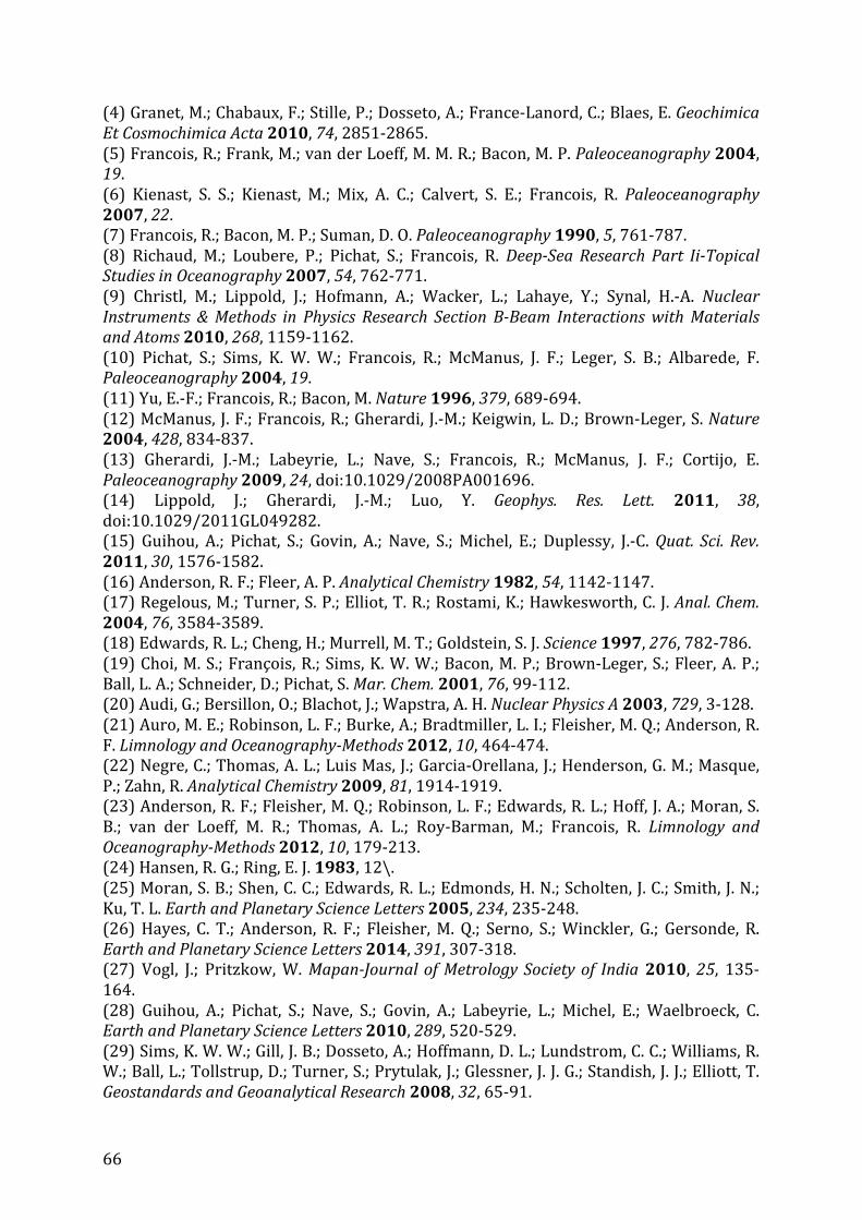
66

(4) Granet, M.; Chabaux, F.; Stille, P.; Dosseto, A.; France‐Lanord, C.; Blaes, E. Geochimica

Et Cosmochimica Acta 2010, 74, 2851‐2865.

(5) Francois, R.; Frank, M.; van der Loeff, M. M. R.; Bacon, M. P. Paleoceanography 2004, 19.

(6) Kienast, S. S.; Kienast, M.; Mix, A. C.; Calvert, S. E.; Francois, R. Paleoceanography

2007, 22. (7) Francois, R.; Bacon, M. P.; Suman, D. O. Paleoceanography 1990, 5, 761‐787.

(8) Richaud, M.; Loubere, P.; Pichat, S.; Francois, R. DeepSea Research Part IiTopical

Studies in Oceanography 2007, 54, 762‐771.

(9) Christl, M.; Lippold, J.; Hofmann, A.; Wacker, L.; Lahaye, Y.; Synal, H.‐A. Nuclear

Instruments & Methods in Physics Research Section BBeam Interactions with Materials

and Atoms 2010, 268, 1159‐1162.

(10) Pichat, S.; Sims, K. W. W.; Francois, R.; McManus, J. F.; Leger, S. B.; Albarede, F.

Paleoceanography 2004, 19.

(11) Yu, E.‐F.; Francois, R.; Bacon, M. Nature 1996, 379, 689‐694.

(12) McManus, J. F.; Francois, R.; Gherardi, J.‐M.; Keigwin, L. D.; Brown‐Leger, S. Nature

2004, 428, 834‐837.

(13) Gherardi, J.‐M.; Labeyrie, L.; Nave, S.; Francois, R.; McManus, J. F.; Cortijo, E.

Paleoceanography 2009, 24, doi:10.1029/2008PA001696. (14) Lippold, J.; Gherardi, J.‐M.; Luo, Y. Geophys. Res. Lett. 2011, 38,

doi:10.1029/2011GL049282.

(15) Guihou, A.; Pichat, S.; Govin, A.; Nave, S.; Michel, E.; Duplessy, J.‐C. Quat. Sci. Rev.

2011, 30, 1576‐1582.

(16) Anderson, R. F.; Fleer, A. P. Analytical Chemistry 1982, 54, 1142‐1147. (17) Regelous, M.; Turner, S. P.; Elliot, T. R.; Rostami, K.; Hawkesworth, C. J. Anal. Chem.

2004, 76, 3584‐3589. (18) Edwards, R. L.; Cheng, H.; Murrell, M. T.; Goldstein, S. J. Science 1997, 276, 782‐786.

(19) Choi, M. S.; François, R.; Sims, K. W. W.; Bacon, M. P.; Brown‐Leger, S.; Fleer, A. P.;

Ball, L. A.; Schneider, D.; Pichat, S. Mar. Chem. 2001, 76, 99‐112. (20) Audi, G.; Bersillon, O.; Blachot, J.; Wapstra, A. H. Nuclear Physics A 2003, 729, 3‐128.

(21) Auro, M. E.; Robinson, L. F.; Burke, A.; Bradtmiller, L. I.; Fleisher, M. Q.; Anderson, R.

F. Limnology and OceanographyMethods 2012, 10, 464‐474. (22) Negre, C.; Thomas, A. L.; Luis Mas, J.; Garcia‐Orellana, J.; Henderson, G. M.; Masque,

P.; Zahn, R. Analytical Chemistry 2009, 81, 1914‐1919. (23) Anderson, R. F.; Fleisher, M. Q.; Robinson, L. F.; Edwards, R. L.; Hoff, J. A.; Moran, S.

B.; van der Loeff, M. R.; Thomas, A. L.; Roy‐Barman, M.; Francois, R. Limnology and

OceanographyMethods 2012, 10, 179‐213. (24) Hansen, R. G.; Ring, E. J. 1983, 12\.

(25) Moran, S. B.; Shen, C. C.; Edwards, R. L.; Edmonds, H. N.; Scholten, J. C.; Smith, J. N.;

Ku, T. L. Earth and Planetary Science Letters 2005, 234, 235‐248. (26) Hayes, C. T.; Anderson, R. F.; Fleisher, M. Q.; Serno, S.; Winckler, G.; Gersonde, R.

Earth and Planetary Science Letters 2014, 391, 307‐318. (27) Vogl, J.; Pritzkow, W. MapanJournal of Metrology Society of India 2010, 25, 135‐

164.

(28) Guihou, A.; Pichat, S.; Nave, S.; Govin, A.; Labeyrie, L.; Michel, E.; Waelbroeck, C.

Earth and Planetary Science Letters 2010, 289, 520‐529.

(29) Sims, K. W. W.; Gill, J. B.; Dosseto, A.; Hoffmann, D. L.; Lundstrom, C. C.; Williams, R.

W.; Ball, L.; Tollstrup, D.; Turner, S.; Prytulak, J.; Glessner, J. J. G.; Standish, J. J.; Elliott, T.

Geostandards and Geoanalytical Research 2008, 32, 65‐91.

67

(30) Fischer, L. B. Analytical Chemistry 1986, 58, 261‐263.

(31) Shiraishi, K.; Takaku, Y.; Yoshimizu, K.; Igarashi, Y.; Masuda, K.; McInroy, J. F.;

Tanaka, G. Journal of Analytical Atomic Spectrometry 1991, 6, 335‐338.

68

Figures

Figure 2.4.1 : Anion‐exchange chromatography separation and purification used by each

of the participating laboratories. HCl concentration is 9N, HNO3 8N and HF 0.13N unless

otherwise stated. Resin types indicated for the last chromatography column of each

laboratory also stand for the previous columns of the laboratory.

1,2,5Waste 3 Th

Pa4

6 U

1) 2*5ml H2O then 2*6ml HCl

2) Sample (20ml HCl) loading

3) 4*3ml HCl

4) 4*3ml HCl+HF

5) 4*3ml HNO3

6) 3*2ml H2O

0.5

ml 1.5

ml

1,2,3Waste 4 Pa

1) 2*5ml H2O

then 2*6ml HCl

2) Pa (12ml HCl)

loading

4) 4*3ml HCl+HF

3) 4*3ml HCl

2) Th (12ml HNO3)

loading

3) 4*3ml HNO3

4) 4*3ml HCl

1) 2*5ml H2O then

2*6ml HNO3

0.5

ml 1.5

ml

0.5

ml 1.5

ml

Eichrom organic

pre-!lter resin

100-150 mesh

Eichrom 1-X8

100-200 mesh

1,2,3Waste 4 Th

2 m

l

1 m

l

1 m

l

AG1-X8

100-200 mesh

1,2,3Waste 4 Th

1) 4*5ml HNO32) Sample (2ml HNO3) loading

3) 2ml HNO3

4) 4*5ml HCl

5) 2*4ml HCl+HF

6) 4*5ml H2O

1,2,3Waste 4Th

Pa 56 U

1) 3*5ml HCl

2) Pa (8ml HCl+HF)

loading3) 4ml HCl+HF

1Waste 2,3 Pa

1) 3*5ml HNO3

2) Th (1ml HNO3)

loading3) 4*1ml HNO34) 2*5ml HCl

1) 5*(5ml HCl + HF then

5ml H2O then 5ml HCl)

2) Sample (2ml HCl) loading3) 1ml HNO3

4) 3*3ml HCl

5) 3*3ml HCl+HF6) 3*4ml 0.1N HCl

2 m

l

2 m

l

2 m

l

AG1-X8

100-200 mesh

1,2,3Waste 4 Th

Pa 56 U

1,2,3Waste 4 Pa

2) Pa (2ml HCl)

loading3) 3*3ml HCl

1) 5*(5ml HCl + HF

then 5ml H2O then

5ml HCl)

4) 4*3ml HCl+HF

2) Th (2ml HNO3)

loading

3) 3*3ml HCl

4) 3*4ml 0.01N HCl

1) 1*5 ml HCl then

3*5ml H2O then

2*2ml HNO3

1,2Waste 3

Th

4.5

ml

2.5

ml

1) 15ml H2O then

15ml HNO32) Sample (5ml HNO3) loading

3) 3*5ml HNO3

4) 6*5ml HCl

5) 4*3ml HCl+HF

6) 20ml 1N HCl

then10ml H2O 1,2,3Waste 4 Th

Pa 56 U

1,2,3Waste 4

Pa

1) 15ml H2O then

15ml HCl

2) Pa (3ml HCl)

loading3) 15ml HCl4) 4*3ml HCl+HF

AG1-X8

100-200 mesh

Pa-Th-U separation Pa puri!cation Th puri!cation

UB

LSCE

LDEO

IUP

4U

69

Figure 2.4.2 : Isotopic ratios measured by each laboratory on thorium and uranium

isotopic reference material. (a) 230Th/232Th measured on IRMM‐035. Certified value is

given as reference, as well as inter‐laboratory MC‐ICP‐MS value from Sims et al 29. (b) 234U/238U measured on NBS‐SRM‐960. Certified value is given as reference. The IUP

group measured NBS‐SRM‐960 twice, on solutions from two different bottles. Error bars

are the maximum between 2SE propagated on the mean (error on the sum of replicate

measurements divided by the number of measurements) and 2SD on sample replicates

(standard deviation of replicate measurements). The number of full chemistry replicates

used to calculate the means is written next to each measurement.

51#

52#

53#

54#

55#

56#

234U/2

38U'

(b)#

Cer.fied# LSCE# UB# LDEO# IUP#

n=1#

n=1#

n=2#

n=3#n=3#

n=3# n=3#

n=3#

n=1#

10#

11#

12#

13#

14#

15#

230Th/2

32Th'

(a)#

70

Figure 2.4.3 : Comparison of the 231Pa concentrations in sediment and UREM11. Results

are expressed by the deviation (%)of the concentrations measured by each laboratory

from the mean of the 4 laboratories. The deviation of the GEOTRACES intercalibration

value from the mean is also given for Geotraces_Sed 23. Note that the GEOTRACES

intercalibration value was not used to compute the mean isotopic concentrations. Error

bars are calculated as in Figure 2 and converted in % from the inter‐laboratory mean.

The number of replicates used to calculate the averages is written next to the error bars.

!10$

!7.5$

!5$

!2.5$

0$

2.5$

5$

7.5$

10$

Margin_Sed$ UREM11$Geotraces_Sed$231Pa$devia>on$from$inter!laboratory$

mean$(%)$

IUP$

LSCE$

UB$

LDEO$

Geotraces$Ref$

2$

2$

2$

3$3$

3$

2$

3$

3$

3$

3$

5$

71

Figure 2.4.4 : Comparison of the (a) thorium and (b) uranium concentrations in

sediment and UREM11. Results are expressed by the deviation (%) of the concentrations

measured by each laboratory from the mean of the 4 laboratories. In (a), the deviation of

the GEOTRACES intercalibration value from the mean is also given for Geotraces_Sed 23.

Note that the GEOTRACES intercalibration value was not used to compute the mean

thorium isotopic concentrations. Error bars are calculated as in Figure 2 and converted

in % from the inter‐laboratory mean. Mean concentrations for each lab were calculated

using three full replicates unless written otherwise on the figure.

!20$

!15$

!10$

!5$

0$

5$

10$

15$

20$

Margin_Sed$ UREM11$

Geotraces_Sed$

Th$devia<on$from$inter!laboratory$

mean$(%)$

Margin_Sed$ UREM11$

Geotraces_Sed$

232Th 230Th

IUP$

LSCE$

UB$

LDEO$

Geotraces$Ref$

(a)$

2$2$

1$5$

!20$

!15$

!10$

!5$

0$

5$

10$

15$

20$

Margin_Sed$ UREM11$

Geotraces_Sed$

U$devia:on$from$inter!laboratory$m

ean$

(%)$

Margin_Sed$ UREM11$

Geotraces_Sed$

238U 234U

IUP$

LSCE$

UB$

LDEO$

(b)$

2$

2$

5$

5$

72

Figure 2.4.5 : Isotopic concentrations obtained at UB after digestion by microwave (white circles) or hotplate (black circles) on (a) UREM11, (b) Geotraces_Sed. Error bars

are calculated as in Figure 2 for microwave measurements. Error bars are 2SE for

hotplate measurements (1 replicate only). Error bars on hotplate measurements on the

Geotraces_Sed sample are small and cannot be distinguished from the data points.

38#

43#

48#

1.5#

2#

2.5#

3#3#

38#

Concentra1on#results#(dpm.g

:1)#

0.054#

0.059#

0.064#0.3#

0.34#

0.38#1.1#

1.2#

1.3#5#

5.4#

5.8#

1.3#

5#

0.38#

1.1#

0.064#

0.3#

(a)# (b)#

UB#Microwave#

UB#Hotplate#

73

Figure 2.4.6 : Concentration deviations of one replicate from the other as a function of

additional time left for 233Pa to decay in the second replicate (see text). Replicates

represented by the square are not full chemistry replicates, but a single Pa fraction that

was measured at different times after U‐Pa separation (10 and 52 days). Replicates

represented by the circles are full chemistry replicates. Numbers indicate the average

concentrations of the replicates (dpm.g‐1). See table S3 for uncertainties on 231Pa

measurements.

!4#

!3#

!2#

!1#

0#

1#

2#

3#

4#

0# 5# 10# 15# 20# 25# 30# 35# 40# 45#

Time#(days)#between#U!Pa#separa;on#of#the#first#and#

second#replicate#

Devia;on#(%)#of#the#concentra;on#of#the#first#

replicate#from#the#second#replicate#

(0.295)#

(0.222)#

(0.246)#

(0.181)#

(0.132)#

(0.176)#

(0.160)#

(0.196)#

74

Tables

Table 2.4.1 : Sediment and spike masses, and digestion steps used by each laboratory. *

H and MW stand for hotplate and microwave respectively. ** White smoke production

indicates that only perchloric acid is left in solution.

Lab Sediment/Spike

addition

Step

n°

Acid addition Temperature

/Pressure

Opened/Closed

beakers *

Duration

LSCE

Sed. Mass: 0.1‐0.2 g

Before digestion:

233Pa: 0.3 pg

229Th: 14 pg

236U: 9 pg

1 2ml HNO3 + 5ml HF 140°C H + closed 12h

2 None (evaporation) 140°C H + opened Until half volume

3 2ml HClO4 + 1ml

HNO3 160°C H + opened

Until white smoke

production **

4 Several 500µl HNO3

rinces 180°C H + opened

Until clear solution

and clean beaker's

sides

UB

Sed. Mass: 0.1 g

After digestion:

233Pa: 0.2 pg

229Th: 50 pg

236U: 1500 pg

Hotplate digestion

1 7ml HNO3 + 3ml HF +

2ml HClO4 180°C H + closed 7‐10h

2 None (evaporation) 180°C H + opened Until ca 1ml left

3 2ml HNO3 + 1ml HF 180°C H + opened

Until complete

evaporation

Microwave digestion

1 6ml HNO3 + 2.5ml HCl

+ 3ml HF 200°C/6MPa MW + closed 2.5h

2 None (evaporation) 150°C H + opened Until ca 1ml left

3 1ml HClO4 + 1ml HF 170°C H + opened

Until complete

evaporation

LDEO


Before digestion:

233Pa: ? pg

229Th: ? pg

236U: ? Pg

1 2ml HNO3 180°C H + opened 2h

2 3ml HClO4 250°C H + opened

Until white smoke

production **

3

1ml HF 150°C H + opened 20h

IUP


Before digestion:

233Pa: 0.8 pg

229Th: 20 pg

236U: 1500 pg

1 3ml HNO3 + 2.5ml HF 120‐160°C MW + closed

Until complete

digestion

2 None 120‐160°C MW + opened

Until complete

evaporation

3 2‐3 drop H3BO3, 2‐3

drop H2O2, 5*6ml

HNO3

215‐220°C H + opened Until evaporation of

each 6ml

75

Table 2.4.2 : Total chemistry yields and separation efficiencies for each of the

laboratories. Max means that elements (U‐Th) separated from the Pa fraction fall below

procedural blanks. Separation efficiency of A from Pa fraction equals the A/Pa ratio in

the sediment divided by the A/Pa ratio in the Pa fraction (where A is either U or Th). The

yield calculated by the LSCE is a rough estimate based on element dilution (acid volume)

and signal during mass spectrometry analysis, and on mass‐spectrometer sensitivity.

Chemistry yield Separation efficiencies

Lab Pa Th U U from Pa fraction Th from Pa fraction

LSCE 40‐80 % 70‐90 % 50‐70 % 1000 500‐2500

UB 90‐98 % 91‐99 % 95‐99 % max max

LDEO 40‐80 % 50‐80 % 60‐90 % 76 max

IUP 10‐50 % 70‐90% 70‐90 % 8000 2000

Table 2.4.3 : Mass‐spectrometer correction intensities, sensitivity and introduction

systems. AS = Abundance sensitivity. Lab Th hydrides U hydrides AS 1 mass Sensitivity (10^6 cps/ppb) Introduction system

LSCE 20 ppm 10 ppm 1‐2 ppm ca 31.25 Apex‐HF

UB 4 ppm negligible 4 ppm ca 18.75 Aridus I desolvating

nebulizer.

LDEO 0.1 ppm 1400 ppm 11 ppm 2.5 Aridus desolvating

nebulizer.

IUP ? ? 270 ppm 0.75‐5 Apex‐HF

Table 2.4.4 : Comparison of concentration results on Geotraces_Sed with the

GEOTRACES intercalibration. Results given in the table are averages of the four

laboratories participating in the study, apart from the second values of 238U and 234U

concentrations, which are averages of MC‐ICP‐MS concentrations only. 231Pa

(dpm.g‐1)

±2D 230Th

(dpm.g‐1)

±2D 232Th

(dpm.g‐1)

±2D 238U

(dpm.g‐1)

±2D 234U

(dpm.g‐1)

±2D

This study 1.20 0.12 5.44 0.12 0.062 0.012 0.312 0.052 0.376 0.064

0.311 0.007 0.351 0.007

GEOTRACES 1.25 0.14 5.53 0.44 0.059 0.010 / /

Table 2.4.5 : Best chemistry methods with respect to efficacy, rapidity, and acid volume used.

Method Efficacy Rapidity Acid volume

Digestion All UB/IUP LDEO

U‐Th‐Pa separation UB IUP LSCE

76

2.4.2 Supporting Information

The supporting information provides additional figures and tables, which further

illustrate the main text. Details concerning the age of the sediment samples and the

mathematical validity of the method for the estimation of 231Pa concentrations are also

provided.

Supporting information

Methodological recommendations for the analysis of sedimentary Pa/Th.

P. Burckel, G. Henry, H‐C Ng, J. Lippold, S. Pichat, M. Roy Barman, F. Thil, J. Gherardi, C.

Waelbroeck, J.F. McManus, L.F. Robinson, B. Antz

1‐Sediment age

The age of Geotraces_Sed is unknown. Because excess protactinium and thorium need to

be decay corrected back to their concentration at the time of sediment deposition for the

calculation of the Pa/Th ratio and because Geotraces_Sed is a near surface sediment, it

was ascribed an age of 500 ± 500 y. Although the age is somewhat arbitrary, it allows

Pa/Th ratio comparison. Margin_Sed was recovered at 72cm from core MD09‐3256Q

(03.55°S/35.39°W, 3537 m water depth) on the Brazilian margin. Its age of 25040 ± 124

(1 SD) y is derived from the linear interpolation of 14C ages determined at 70 and 74 cm

(26189 ± 119 (1 SD) y and 23890 ± 128 (1 SD) y respectively) and converted to calendar

age using the Marine13 calibration curve. Because of the age inversion (deepest level

being younger than the shallowest), Margin_Sed might have been deposited by a

turbidite.

2‐Estimation of the sedimentary 231Pa concentration

To circumvent the problem of the 233Pa decay in the measurement of sedimentary 231Pa

concentrations, one 233Pa spiked 231Pa standard must be U‐Pa separated and measured

at the same time as the protactinium fraction of the sediment samples.

Consider a protactinium sample being measured on mass spectrometer and containing

N233Pa, and N233U atoms of 233Pa and 233U respectively as well as N231 atoms of 231Pa.

This sample can be either a 233Pa spiked 231Pa standard solution (known 231Pa and

unknown 233Pa) or dissolved sediment (unknown 231Pa and 233Pa). In both cases, the

233Pa/231Pa ratio R measured on mass spectrometer follows this equation:

77

� =�!"#

�!""�� + �!""� !"## !"#$

= �!"# ∗ �!"

�!""�� ∗ �!" + �!""� ∗ �!

=�!"# ∗ �!"

�!"" ∗ ( �!!∗!!) ∗ �!" + (1 − �

!!∗!! ∗ �!)

=�!"#

�!"" ∗ ( �!!∗!!) + (1 − �!!∗!! ∗ �)

=�!"#

�!"" ∗ �(�2,�)(1)

where N233 is the number of atoms of 233(Pa + U), SU and SPa are the mass spectrometer

counts per atom (so that α is the ratio of ionization efficiencies of U and Pa) of uranium

and protactinium respectively, λ the 233Pa decay constant and t2 the time between

column chromatography and analysis on mass spectrometer.

Because there should not be any Pa loss during digestion, and because column chemistry

does not alter the 233Pa/231Pa ratio, equation (1) can be written:

� =�!"#�

�!""� ∗ �!!∗!! ∗ �(�2,�)

=�!"#�

�!""� ∗ �(�1, �2,�) (2)

where t1 is the time between spike creation and column chromatography, N231i and

N233i the initial number of atoms of 231Pa and 233Pa respectively (i.e. atoms in the mass of

sediment or 231Pa standard and in the spike). The term B depends on the timing of the U‐

Pa separation with respect to spike production and mass spectrometer measurement (t1

and t2), as well as on the ionization efficiency ratio α. Sediments and spiked 231Pa

standards are separated and measured at the same time on mass spectrometer and

therefore have identical B values.

We can then easily find the sample’s 231Pa concentrations. Consider first a standard

solution (Std) with known N231i(Std). From equation (2) we have:

� �� =�!"#�(��)

�!""�(��) ∗ �(�1, �2,�)

78

=�!"#�(��)

M!"#$%(Std) ∗ [ ��

233 ]�∗ B(t1, t2,α)

[ �� !"" ]! ∗ B t1, t2,α =

�231� ��

MSpike Std ∗ � ��(3)

where [233Pa]i is the initial concentration of the 233Pa spike (i.e. after spike production)

and Mspike(Std) is the mass of 233Pa spike in the standard solution.

Consider now a spiked sediment sample (Smp) with unknown N231i(Smp) that was Pa

purified by column chromatography at the same time as the spiked 231Pa standard. From

equation (2) and equation (3) we can eliminate the unknown [233Pa]i and B and write:

� �� =�!"#�(��)

�!""�(��) ∗ �(�1, �2,�)=

�!"#�(��)

M!"#$% Smp ∗ ��

233

�∗ �(�1, �2,�)

=�!"#�(��)

M!"#$%(Smp)∗ � �� ∗

M!"#$%(Std)

�!"#�(��)

�� !"#

!"# =

� �� ∗M!"!"# Smp ∗ �!"#�(��)

� �� ∗M!"#$%(Std)

�!"#

(4)

where [231Pa]sed is the 231Pa concentration of the sediment and Msed the sediment’s

mass. R(Smp) is measured, MSpike(Smp) and Msed are known and the rest of the terms are

known from the standard solution. We can therefore calculate the sediment’s 231Pa

concentration.

79

Figure 2.4.S1 : Illustration of the coning and quartering method. First, a) the sediment is poured on drawing paper by applying a swirling movement to the wrist in order to form

a dome then b) the dome is divided in four and c) the opposite quarters are gathered.

The resulting sediment piles (2, 3) and the initial sediment (1) are expected to be

homogeneous.

Top viewSide view

a)

b)

c)

1

2

3

Sediment

1

1, 2 and 3

homogeneous

80

Figure 2.4.S2 : Sediment and UREM11 232Th concentration results for each of the participating laboratories. Note that the y axis range for each sample is of around 25% of

the sample’s mean concentration. This allows to compare the inter and intra‐laboratory

concentration variability of the samples. Hence care should be taken when comparing

absolute concentrations, as the y axis is often split and magnified for some samples.

Circles represent the UREM11, squares the Geotraces_Sed and diamonds the Margin_Sed

samples. Error bars are 2SE.

81

Figure 2.4.S3 : Sediment and UREM11 230Th concentration results for each of the participating laboratories. Note that the y axis range for each sample is of around 25% of






82

Figure 2.4.S4 : Sediment and UREM11 238U concentration results for each of the

participating laboratories. Note that the y axis range for each sample is of around 25% of






83

Figure 2.4.S5 : Sediment and UREM11 234U concentration results for each of the participating laboratories. Note that the y axis range for each sample is of around 25% of






84

Figure 2.4.S6 : Sediment and UREM11 231Pa concentration results for each of the

participating laboratories. Note that the y axis range for each sample is of around 25% of






85

Figure 2.4.S7 : Mean Pa/Th values obtained by each of the participating labs. Note that the y axis range for both samples is of around 25% of the sample’s mean Pa/Th. This

allows to compare the inter‐laboratory Pa/Th variability of the samples. Hence care

should be taken when comparing absolute Pa/Th values, as the y axis is split and

magnified. Squares represent the Geotraces_Sed and diamonds the Margin_Sed samples.

2 sigma error is calculated based on the maximum between 2 SE and 2 SD of replicate

concentration measurements and does not include the uncertainty on the R value (set to

0.5).

0.05$

0.07$

0.09$0.2$

0.22$

0.24$

0.09$

0.2$

Pa/Th$

LSCE$ UB$ LDEO$ IUP$

Margin_Sed$

Geotraces_Sed$

86

Table 2.4.S1 : Isotopic ratio measurements (×106) on isotopic reference material NBS‐

SRM‐960 and IRMM‐035. 234U/238U measurements by the IUP were done on NBS‐

SRM‐960 from two different bottles. The value given by Sim et al for the 230Th/232Th

ratio of IRMM‐035 is also displayed.

NBS‐SRM‐960 IRMM‐035

Lab 234U/238U ± 2SE 230Th/232Th ± 2SE

Certified 52.841 0.082 11.481 0.078

Sims et al., 2008 / / 11.38 0.096

LSCE 53.003 0.110 11.111 0.098

53.029 0.101 11.266 0.087

53.063 0.105 11.313 0.116

UB 52.805 0.142 11.203 0.105

52.890 0.112 11.315 0.081

52.797 0.147 11.336 0.063

LDEO 54.620 3.048 13.462 1.842

56.393 3.159 13.351 2.470

13.535 2.631

IUP 54.624 0.909 14.710 1.334

52.977 0.886

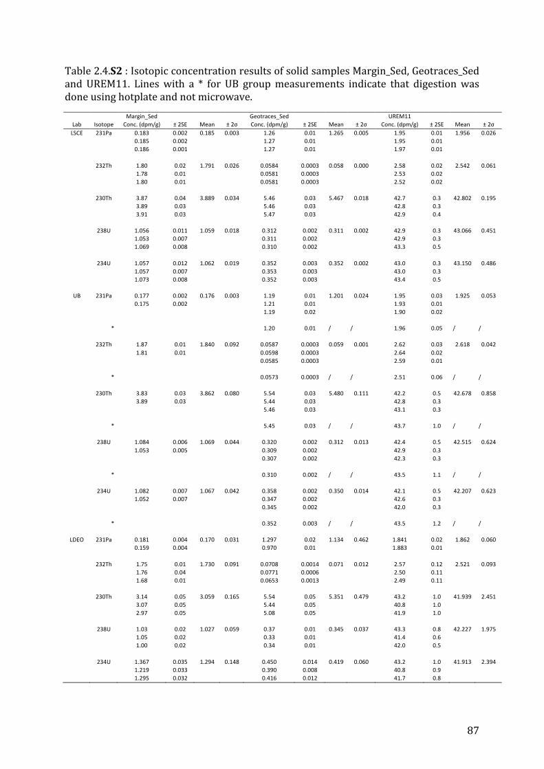
87

Table 2.4.S2 : Isotopic concentration results of solid samples Margin_Sed, Geotraces_Sed

and UREM11. Lines with a * for UB group measurements indicate that digestion was

done using hotplate and not microwave.

Margin_Sed Geotraces_Sed UREM11

Lab Isotope Conc. (dpm/g) ± 2SE Mean ± 2σ Conc. (dpm/g) ± 2SE Mean ± 2σ Conc. (dpm/g) ± 2SE Mean ± 2σ

LSCE 231Pa 0.183 0.002 0.185 0.003 1.26 0.01 1.265 0.005 1.95 0.01 1.956 0.026

0.185 0.002 1.27 0.01 1.95 0.01

0.186 0.001 1.27 0.01 1.97 0.01

232Th 1.80 0.02 1.791 0.026 0.0584 0.0003 0.058 0.000 2.58 0.02 2.542 0.061

1.78 0.01 0.0581 0.0003 2.53 0.02

1.80 0.01 0.0581 0.0003 2.52 0.02

230Th 3.87 0.04 3.889 0.034 5.46 0.03 5.467 0.018 42.7 0.3 42.802 0.195

3.89 0.03 5.46 0.03 42.8 0.3

3.91 0.03 5.47 0.03 42.9 0.4

238U 1.056 0.011 1.059 0.018 0.312 0.002 0.311 0.002 42.9 0.3 43.066 0.451

1.053 0.007 0.311 0.002 42.9 0.3

1.069 0.008 0.310 0.002 43.3 0.5

234U 1.057 0.012 1.062 0.019 0.352 0.003 0.352 0.002 43.0 0.3 43.150 0.486

1.057 0.007 0.353 0.003 43.0 0.3

1.073 0.008 0.352 0.003 43.4 0.5

UB 231Pa 0.177 0.002 0.176 0.003 1.19 0.01 1.201 0.024 1.95 0.03 1.925 0.053

0.175 0.002 1.21 0.01 1.93 0.01

1.19 0.02 1.90 0.02

* 1.20 0.01 / / 1.96 0.05 / /

232Th 1.87 0.01 1.840 0.092 0.0587 0.0003 0.059 0.001 2.62 0.03 2.618 0.042

1.81 0.01 0.0598 0.0003 2.64 0.02

0.0585 0.0003 2.59 0.01

* 0.0573 0.0003 / / 2.51 0.06 / /

230Th 3.83 0.03 3.862 0.080 5.54 0.03 5.480 0.111 42.2 0.5 42.678 0.858

3.89 0.03 5.44 0.03 42.8 0.3

5.46 0.03 43.1 0.3

* 5.45 0.03 / / 43.7 1.0 / /

238U 1.084 0.006 1.069 0.044 0.320 0.002 0.312 0.013 42.4 0.5 42.515 0.624

1.053 0.005 0.309 0.002 42.9 0.3

0.307 0.002 42.3 0.3

* 0.310 0.002 / / 43.5 1.1 / /

234U 1.082 0.007 1.067 0.042 0.358 0.002 0.350 0.014 42.1 0.5 42.207 0.623

1.052 0.007 0.347 0.002 42.6 0.3

0.345 0.002 42.0 0.3

* 0.352 0.003 / / 43.5 1.2 / /

LDEO 231Pa 0.181 0.004 0.170 0.031 1.297 0.02 1.134 0.462 1.841 0.02 1.862 0.060

0.159 0.004 0.970 0.01 1.883 0.01

232Th 1.75 0.01 1.730 0.091 0.0708 0.0014 0.071 0.012 2.57 0.12 2.521 0.093

1.76 0.04 0.0771 0.0006 2.50 0.11

1.68 0.01 0.0653 0.0013 2.49 0.11

230Th 3.14 0.05 3.059 0.165 5.54 0.05 5.351 0.479 43.2 1.0 41.939 2.451

3.07 0.05 5.44 0.05 40.8 1.0

2.97 0.05 5.08 0.05 41.9 1.0

238U 1.03 0.02 1.027 0.059 0.37 0.01 0.345 0.037 43.3 0.8 42.227 1.975

1.05 0.02 0.33 0.01 41.4 0.6

1.00 0.02 0.34 0.01 42.0 0.5

234U 1.367 0.035 1.294 0.148 0.450 0.014 0.419 0.060 43.2 1.0 41.913 2.394

1.219 0.033 0.390 0.008 40.8 0.9

1.295 0.032 0.416 0.012 41.7 0.8

88

Table 2.4.S2: Continued. Margin_Sed Geotraces_Sed UREM11

Lab Isotope Conc. (dpm/g) ± 2SE Mean ± 2σ Conc. (dpm/g) ± 2SE Mean ± 2σ Conc. (dpm/g) ± 2SE Mean ± 2σ

IUP 231Pa 0.178 0.008 0.182 0.008 1.22 0.01 1.219 0.022 1.98 0.02 1.958 0.077

0.182 0.003 1.23 0.01 1.94 0.02

0.186 0.003 1.21 0.01 1.91 0.01

2.01 0.01

1.95 0.01

232Th 1.89 0.048 1.799 0.271 0.0589 0.0012 0.060 0.001 2.43 0.05 / /

1.86 0.050 0.0602 0.0014

1.64 0.081 0.0597 0.0012

230Th 3.82 0.06 3.623 0.352 5.48 0.09 5.478 0.051 41.7 0.7 41.566 1.753

3.49 0.06 5.49 0.10 41.9 0.6

3.55 0.07 5.47 0.08 42.1 0.6

40.0 0.6

42.2 0.6

238U 1.080 0.006 1.090 0.021 0.276 0.002 0.282 0.037 42.6 0.2 42.310 2.334

1.101 0.006 0.267 0.002 40.3 0.2

1.090 0.006 0.302 0.002 42.7 0.2

43.3 0.2

42.7 0.2

234U 1.122 0.008 1.114 0.014 0.385 0.004 0.382 0.007 44.3 0.2 43.529 1.803

1.110 0.010 0.379 0.003 42.1 0.2

1.109 0.012 0.382 0.006 43.6 0.3

44.3 0.2

43.4 0.3

89

Table 2.4.S3 : 231Pa concentration of replicate samples (e.g. 1 a and 1 b) measured at

different times t between U‐Pa separation and mass spectrometer analysis. Sample 8 a

and 8 b are not full sediment replicates, but a single 231Pa/233(Pa+U) solution measured

at different times after U‐Pa separation.

Sample n° 231Pa (dpm.g-1) ± 2 sigma t (days)

1 a 0.296 0.002 6

1 b 0.294 0.003 13

2 a 0.220 0.002 6

2 b 0.225 0.003 13

3 a 0.245 0.002 6

3 b 0.247 0.002 13

4 a 0.184 0.001 6

4 b 0.178 0.002 20

5 a 0.132 0.001 6

5 b 0.133 0.002 20

6 a 0.176 0.002 6

6 b 0.176 0.001 20

7 a 0.159 0.002 6

7 b 0.162 0.002 27

8 a 0.197 0.001 10

8 b 0.194 0.001 52

90

Table 2.4.S4 : Mean Pa/Th results for each of the labs. 2 sigma error is calculated based

on the maximum between 2 SE and 2 SD of replicate concentration measurements and

does not include the uncertainty on the R value (set to 0.5).

Margin_Sed Geotraces_Sed

Pa/Th 2 sigma Pa/Th 2 sigma

LSCE 0.064 0.002 0.234 0.003

UB 0.061 0.002 0.221 0.007

LDEO 0.080 0.006 0.214 0.019

IUP 0.069 0.010 0.225 0.005

91

Table 2.4.S5 : Acid volumes used by each lab for digestion and elution by column

chromatography. Only acids more concentrated than 2N are considered.

Lab HNO3 (ml) HCl (ml) HF (ml) HClO4 (ml) HCl + HF (ml) Total (ml)

Digestion LSCE 5 0 5 2 0 12

UB 6 2.5 4 1 0 13.5

LDEO 2 0 1 3 0 6

IUP 33 0 2.5 0 0 35.5

U‐Th‐Pa

separation

LSCE 41 45 0 0 12 98

UB 36 60 0 0 24 120

LDEO 5 82 0 0 71 158

IUP 30 60 0 0 24 114

93

Chapter 3 : Timing of Oceanic circulation changes in the

Atlantic during the last glacial

3.1 Introduction

As discussed in chapter I, climate models are able to simulate a southward shift of the

ITCZ, either in response to a slowdown of the AMOC (Kageyama et al., 2009), or through

the increased extent of sea ice or ice sheets (Chiang and Bitz, 2005) that generate a cold

SST anomaly in the northern tropics, shifting the tropical rain belt to the south.

However, it remains unclear which of these processes triggered the southward ITCZ

shifts associated with Greenland stadials of the last glacial.

Southward shifts of the ITCZ are associated with increased precipitation in northern

South America, and are therefore recorded as Ti/Ca peaks in marine sediments of the

Brazilian margin (Jaeschke et al., 2007). As deep western boundary currents also affect

our sediment cores, I directly compare oceanic circulation and ventilation proxies to the

precipitation signal measured in core MD09‐3257 (~2300 m depth), to precisely assess

the phase relationship between AMOC variations and ITCZ shifts. A large Pa/Th increase

occurs before the onset of the precipitation events associated with Heinrich Stadial 2

and Heinrich Stadial 4. In order to assess the timing of the AMOC slowdown with respect

to the ITCZ shift, I build a robust age model based on correlation of the Ti/Ca signal of

our core with another nearby 14C dated core, and with a U‐Th dated South American

speleothem that recorded periods of increased precipitation as decreases in the δ18O

record. As seen in Chapter 2, the Pa/Th data I produced are very precise and can

therefore be used to reliably determine the start of the AMOC slowdown, and as sharp

Ti/Ca peaks mark periods of increased precipitation, I precisely determine the lead of

the AMOC slowdown in terms of core length for HS2 and HS4. Converting the lead

expressed as a length in the core into a lead expressed as a time interval, I find that the

decreased AMOC intensity preceded the precipitation events by 1420 ± 250 (1σ) y and

690 ± 180 (1σ) y for HS2 and HS4 respectively. Results are presented in the article

entitled “Atlantic Ocean circulation changes preceded millennial tropical South America

rainfall events during the last glacial”.

In the last section of this chapter, I provide another potential explanation for the Pa/Th

rise occurring prior to precipitation events, which does not affect the conclusions of the

article. I also discuss a recent study (Lynch‐Stieglitz et al., 2014) that concluded that the

upper circulation cell of the AMOC did not slowdown during Heinrich Stadial 2 and 3, in

contradiction with my results.

94

3.2 Atlantic Ocean circulation changes preceded millennial tropical

South America rainfall events during the last glacial

This article has been submitted to Nature Geoscience and Proceedings of the National

Academy of Sciences. Unfortunately, with 1/3 and 1/2 positive reviews, the article was

not accepted. The format will be changed and the article submitted to Geophysical

Research Letters before the defense.

95

Atlantic Ocean circulation changes preceded millennial tropical South America

rainfall events during the last glacial

Pierre Burckela*, Claire Waelbroecka, Jeanne Marie Gherardia, Sylvain Pichatb, Helge Arzc,

Joerg Lippoldd, Trond Dokkene, and François Thila

aLSCE/IPSL, Laboratoire CNRS‐CEA‐UVSQ, Bât.12, avenue de la Terrasse, F‐91198 Gif

sur Yvette, France

bLaboratoire de Géologie de Lyon (LGL‐TPE), Ecole Normale Supérieure de Lyon, 46


cLeibniz‐Institute for Baltic Sea Research, Seestrasse 15, D‐18119 Rostock, Germany

dOeschger Centre for Climate Change Research, Institute of Geological Sciences,

University of Bern, Zähringerstrasse 25, CH‐3012, Bern, Switzerland

eBjerknes Centre for Climate Research, Department of Earth Sciences, University of

Bergen, Allégt. 55, N‐5007 Bergen

*Corresponding author: [email protected] +33 (0)1.69.82.43.47

Keywords : Heinrich, Dansgaard‐Oeschger, MIS3, AMOC, ITCZ, Pa/Th

96

Abstract

During the last glacial period, Greenland’s climate experienced millennial‐scale shifts

between cold (stadial) and warm (interstadial) phases that were accompanied by ocean

circulation changes characterized by reduced Atlantic Meridional Overturning

Circulation during stadials. Here, we present new 231Pa/230Th data from a deep‐sea

sediment core retrieved off North‐East Brazil demonstrating that slowdowns of the

Atlantic Meridional Overturning Circulation preceded the large southward shifts of the

intertropical convergence zone that took place during last glacial stadial periods. We

reliably determine that the Atlantic Meridional Overturning Circulation started to

slowdown 1420 ± 250 (1σ) y and 690 ± 180 (1σ) y before the onset of two large

precipitation events, associated with Heinrich stadials, recorded in South America. Our

results thus bring unprecedented evidence that Atlantic Meridional Overturning

Circulation changes could be the origin of the observed precipitation events. In addition,

we propose a new mechanism that explains the differences in the extent and timing of

Atlantic Meridional Overturning Circulation slowdowns associated with shorter and

longer stadial periods.

97

Introduction

Both paleoproxy records and numerical modeling indicate that the tropical and

northern North Atlantic regions are tightly linked on centennial to millennial timescales.

Sediment records from the Cariaco Basin show that tropical Atlantic Ocean and

atmosphere changes correlate with variations in the North Atlantic region since the last

glacial period (1‐4). Some modeling studies have suggested that these regions may be

connected via a coupled atmosphere‐surface ocean mechanism (5, 6), whereas other

numerical simulations using fully coupled atmosphere‐ocean models have indicated that

a reduction in the Atlantic Meridional Overturning Circulation (AMOC) flow rate could

induce a southward displacement of the Intertropical Convergence Zone (ITCZ) (7‐9).

The western side of the tropical Atlantic is a key region to study the mechanisms behind

millennial‐scale tropical atmospheric changes. Indeed, during the last glacial, millennial

variability in precipitation over tropical South America is recorded in various archives

such as marine or lake sediments and speleothems (4, 10‐17). Precipitation changes are

interpreted as latitudinal shifts of the ITCZ, and appear to covary over South America in

the 0‐30°S latitude band east of the Andes. Moreover, the western side of the tropical

Atlantic is the locus of the western boundary currents and is therefore ideal to monitor

changes in the AMOC flow rate (18). Cores MD09‐3257 (04°14.69’S, 36°21.18’W, 2344m

water depth) and GeoB3910 (04°14.7’S, 36°20.7’W, 2362m water depth) were retrieved

from approximately the same location and depth on the North Eastern Brazilian margin

(Fig. 1). At present, the cores site is bathed by the upper limb of the North Atlantic Deep

Water, originating from the North Atlantic Ocean and circulating between 1200 and

2500m depth, with a maximum circulation intensity of ca. 11 Sv at ~1500m (19).

Numerous studies indicate that northern‐sourced deep water flowed at shallower depth

during the last glacial compared to modern times (20‐22). Hence, the location of the

sediment cores studied here is ideal to monitor past changes in the AMOC upper

circulation cell, as well as their relation to millennial‐scale precipitation events that are

associated with the shifts in the ITCZ position.

Under modern conditions, the Brazilian northeastern region, called Nordeste (Fig. 1), is

a semi‐arid region where precipitation is controlled by the position of the ITCZ. Periods

of high precipitation (March‐April) in the Nordeste occur when the ITCZ is at its

southernmost position and the interhemispheric sea surface temperatures (SST)

gradient is the weakest (23). During boreal summer, the SST gradient steepens and the

ITCZ moves northward, following the position of maximum SST above which convection

occurs.

98

During the last glacial, millennial‐scale variability in precipitation led to periods of

increased rainfall in the Nordeste. Increased precipitation is marked by a decrease in

δ18O in South American speleothems (10, 11, 14, 24‐26) and increased sedimentary

Ti/Ca ratios in a marine sediment core off the northeastern Brazilian coast (12) (SI

Appendix section A, and Figs. S1‐S2).

Precipitation events recorded in South American speleothems can be considered

synchronous within age uncertainties (SI Appendix section B, and Figs. S3‐S4). These

precipitation events were shown to take place during cold stadial periods recorded in

Greenland ice cores (10, 11, 14, 25‐28). In what follows, we call Heinrich stadials the six

stadials characterized by the occurrence of Heinrich events, i.e. thick layers of ice rafted

detritus in mid‐ to high‐latitude North Atlantic sediments, indicative of massive iceberg

surges. We define PE0 as the precipitation event occurring during the Younger Dryas,

and PE1 to PE5, those occurring during Heinrich stadials 1 to 5, respectively (SI

Appendix Fig. S3).

Results

Using 14C dating, we could verify that precipitation events in marine cores are

synchronous with precipitation events in speleothems for the 10‐38 cal. ky BP (ka

hereafter) period (Fig. 2 and Methods). This led us to synchronize to speleothems δ18O

records the two high Ti/Ca events, PE4 and 5, which occur during the 38‐50 ka period,

i.e. beyond the range of precise 14C dating. Doing so, we observe that all the small

precipitation events seen in marine sediments between 38 and 50 ka are synchronous

with those seen in speleothems, which further confirms the synchronism between

precipitation events recorded in marine sediments and speleothems. Importantly, the

resulting marine cores age scales are entirely radiometric and based on regional

correlations, and hence completely independent from the Greenland ice core

chronology.

Comparing the Ti/Ca marine records with Greenland air temperature record on their

respective independent calendar age scales, we observe that periods of increased

precipitation over our study area take place during cold periods over Greenland (Fig. 3a,

d). This is the case for both large precipitation events PE2 to PE5 and smaller ones

(Ti/Ca <0.2) associated with the stadials preceding Dansgaard Oeschger (DO) 5, 6, 7, 10

and 11. The only exception is the small precipitation event following PE3 in our

sediment core that appears to coincide with the DO4 interstadial. However, the timing of

this precipitation event can be reconciled with that of the stadial preceding DO3 within

age model uncertainties. Some studies have shown that millennial‐scale precipitation

events seen in marine sediment cores for the period covered by 14C dating occurred

99

during Greenland stadials (e.g. ref. (12)). However, these studies then assumed that

Greenland stadials and tropical precipitation events were also synchronous beyond 40

ka. Moreover, in some cases, tropical marine records were dated by assuming that the

tropical climate and Greenland signals were synchronous over the entire last glacial (4,

29). Such dating methods preclude establishing the sequence of events and determining

which component of the climate system has triggered the observed millennial climate

variability. In contrast, by building a radiometric age scale for our low latitude marine

records that is entirely independent from the Greenland ice core age scale, we are able

to assess the respective timing of the different climatic and ocean circulation signals

recorded in Greenland and South America 0‐30°S latitudinal band.

Sedimentary 231Pa/230Th (Pa/Th hereafter) can be used to record changes in AMOC flow

rate (22, 30‐32) (Methods). In effect, at present, Pa/Th in the western tropical Atlantic is

mainly controlled by oceanic circulation (33). While caveats may apply to this proxy in

regions of high particle flux, we could verify that during the last glacial, the main drivers

of the Pa/Th variability in our core remained the changes in oceanic circulation intensity

(Methods). Pa/Th rises from approximately modern day values prior to precipitation

events PE2 and PE4, to values close to that of the production ratio (0.093) at their onset

(Fig. 3b). This indicates that the overlying water mass flow rate was strongly reduced at

the onset of PE2 and PE4. Similarly, decreased flow rate accompanied the smaller

precipitation events related to DO stadials, as illustrated by the increase in Pa/Th values

during each DO related stadial, namely 6 and 7, for which we have the data. Moreover,

increases in Pa/Th are synchronous with decreases in the δ13C of the benthic foraminifer

Cibicides wuellerstorfi (Fig. 3c) that can be interpreted as reflecting reduced bottom

water ventilation (Methods). The concurrent decrease in benthic δ13C and increase in

Pa/Th ratio in our cores thus indicates longer bottom water residence times and lower

ventilation at 2300 m depth on the north‐east Brazilian margin during millennial

precipitation events. Our marine records thus unambiguously indicate that major

decreases in the flow rate of the AMOC upper circulation cell took place before the main

and during the small millennial precipitation events.

Sedimentary Pa/Th starts rising before the Ti/Ca increase associated with PE4 and PE2

in core MD09‐3257 (Fig. 3b, d, SI Appendix section C, and Fig. S9). Because Ti/Ca and

Pa/Th values were measured in the same core, the leads are directly measurable in

terms of core length: Pa/Th starts rising nearly 5 cm before the onset of PE4 and more

than 9 cm before the onset of PE2. Converting these depths intervals into time intervals,

the lead of the Pa/Th signal with respect to the Ti/Ca signal is estimated to be 690 ± 180

(1σ) y and 1,420 ± 250 (1σ) y at the onsets of PE4 and PE2, respectively. The AMOC

slowdown therefore starts significantly earlier than the large precipitation events

100

observed in the 0‐30°S latitudinal band in South America. While the sequence of events

is straightforward for PE4 and PE2, the phasing between AMOC slowdowns and small

precipitation events related to DO stadials is more difficult to assess. Indeed, the Pa/Th

signal seems to rise before the start of the Ti/Ca peak for precipitation events associated

with stadials preceding DO 7 and 6 (Fig. 3). However, if the AMOC slowdown indeed

precedes small precipitation events, then the time lag between the beginning of the

AMOC slowdown and of the precipitation event is much smaller than for precipitation

events associated with Heinrich stadials (Fig. S9).

Discussion

Our data bring new constraints on the possible trigger mechanisms of the millennial

precipitation events observed in the 0‐30°S latitudinal band in South America during the

last glacial. Our results demonstrate that precipitation events corresponding to Heinrich

stadials over our study area occurred 500 to 1,700 y after a slowdown of the AMOC

upper circulation cell. Thus, there could be a causal link between the AMOC slowdowns

and ITCZ shifts, that is, the observed slowdowns could trigger the precipitation events.

Climate models indeed show that an AMOC slowdown causes a decrease in

interhemispheric oceanic heat transport (see ref. (34) for a review), which results in

negative SST anomalies in the Northern and positive SST anomalies in the Southern

extratropics. The SST anomalies are then propagated equatorwards inducing a

southward ITCZ shift (8). This mechanism could thus have led to the southward shift of

the convection zone and explain the observed sequence of events (arrow 1a in Fig. 4).

However, other modeling studies produced southward ITCZ shifts in response to

extended high‐latitudes ice sheets or sea ice cover (5, 6), without any change in the

AMOC. In these models, surface cooling in the North Atlantic and Nordic Seas induces

the progression of low SST towards the ITCZ latitudes, leading to a southward

displacement of the ITCZ after only a few years. Interestingly, the records in Fig. 3 do not

support this mechanism as sole cause for the observed precipitation events since PE2

starts after the beginning of Heinrich stadial 2 cold periods above Greenland (arrow 1b

in Fig. 4). Extended ice‐sheet or sea‐ice cover could however be responsible for the small

precipitation events. These events indeed occur synchronously with short stadials

between DO events and the associated Pa/Th signal, although indicating a strong AMOC

slowdown, does not feature the same obvious lead with respect to the Ti/Ca signal as for

the main precipitation events. Smaller increases in the Ti/Ca signal may reflect a more

northerly final position of the ITCZ and different mechanisms could be at the origin of

large and small precipitation events. The latter could reflect a small southward ITCZ

shift resulting from northern tropics sea surface cooling in response to an extension of

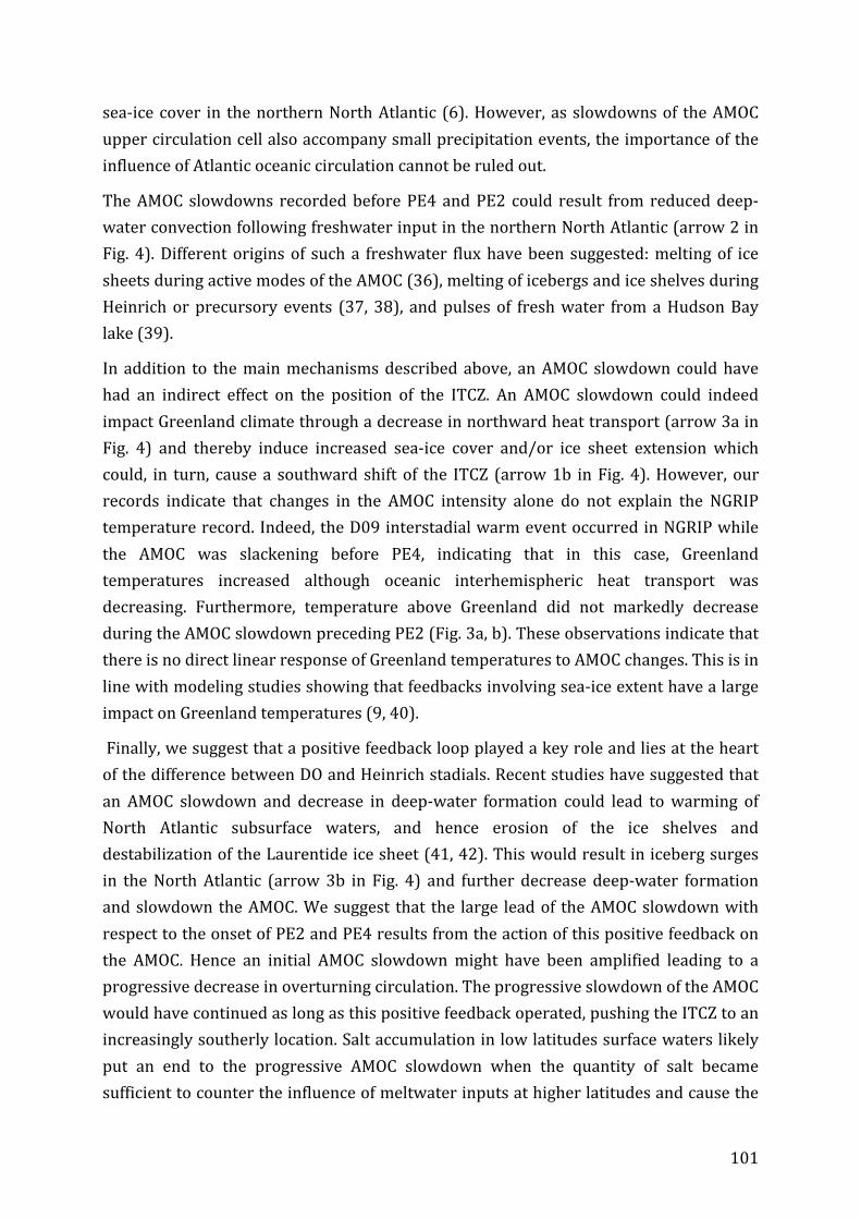
101

sea‐ice cover in the northern North Atlantic (6). However, as slowdowns of the AMOC

upper circulation cell also accompany small precipitation events, the importance of the

influence of Atlantic oceanic circulation cannot be ruled out.

The AMOC slowdowns recorded before PE4 and PE2 could result from reduced deep‐

water convection following freshwater input in the northern North Atlantic (arrow 2 in

Fig. 4). Different origins of such a freshwater flux have been suggested: melting of ice

sheets during active modes of the AMOC (36), melting of icebergs and ice shelves during

Heinrich or precursory events (37, 38), and pulses of fresh water from a Hudson Bay

lake (39).

In addition to the main mechanisms described above, an AMOC slowdown could have

had an indirect effect on the position of the ITCZ. An AMOC slowdown could indeed

impact Greenland climate through a decrease in northward heat transport (arrow 3a in

Fig. 4) and thereby induce increased sea‐ice cover and/or ice sheet extension which

could, in turn, cause a southward shift of the ITCZ (arrow 1b in Fig. 4). However, our

records indicate that changes in the AMOC intensity alone do not explain the NGRIP

temperature record. Indeed, the D09 interstadial warm event occurred in NGRIP while

the AMOC was slackening before PE4, indicating that in this case, Greenland

temperatures increased although oceanic interhemispheric heat transport was

decreasing. Furthermore, temperature above Greenland did not markedly decrease

during the AMOC slowdown preceding PE2 (Fig. 3a, b). These observations indicate that

there is no direct linear response of Greenland temperatures to AMOC changes. This is in

line with modeling studies showing that feedbacks involving sea‐ice extent have a large

impact on Greenland temperatures (9, 40).

Finally, we suggest that a positive feedback loop played a key role and lies at the heart

of the difference between DO and Heinrich stadials. Recent studies have suggested that

an AMOC slowdown and decrease in deep‐water formation could lead to warming of

North Atlantic subsurface waters, and hence erosion of the ice shelves and

destabilization of the Laurentide ice sheet (41, 42). This would result in iceberg surges

in the North Atlantic (arrow 3b in Fig. 4) and further decrease deep‐water formation

and slowdown the AMOC. We suggest that the large lead of the AMOC slowdown with

respect to the onset of PE2 and PE4 results from the action of this positive feedback on

the AMOC. Hence an initial AMOC slowdown might have been amplified leading to a

progressive decrease in overturning circulation. The progressive slowdown of the AMOC

would have continued as long as this positive feedback operated, pushing the ITCZ to an

increasingly southerly location. Salt accumulation in low latitudes surface waters likely

put an end to the progressive AMOC slowdown when the quantity of salt became

sufficient to counter the influence of meltwater inputs at higher latitudes and cause the

102

resumption of the oceanic inter‐hemispheric heat transport (36, 43 , 44). The

reactivation of the overturning circulation would then cause the ITCZ to move back to its

original, more northerly, position. We propose that, in contrast to the progressive

amplification of the AMOC slowdown that took place during Heinrich stadials, the AMOC

slowdowns that occurred during the stadials preceding DO events did not trigger the

afore described positive feedback. As a result, both the decrease in AMOC and latitudinal

shift in the ITCZ taking place during DO stadials remained limited. As the feedback is

only triggered during Heinrich Stadials, iceberg discharges would be limited during

stadials preceding DO events. The proposed mechanism is therefore consistent with the

observed higher IRD content of North Atlantic sediments during Heinrich Stadials than

during DO stadials.

Moreover, recent data from Antarctic ice cores show that atmospheric CO2 progressively

increased during each Heinrich stadial but remained constant or slightly decreased

during DO stadials (45). The fact that the atmospheric CO2 trend is drastically different

during DO stadials than during Heinrich stadials points to the existence of an additional

feedback involving the carbon cycle during Heinrich stadials, that does not operate

during DO stadials, very likely related to the large changes in ocean circulation

demonstrated by our data.

Conclusions

Our results demonstrate that the AMOC upper circulation cell experienced marked

slowdowns 500 to 1,700 years before major tropical South American precipitation

events that occurred during Heinrich stadials and corresponded to southward shifts of

the ITCZ. Our data thereby provide the first unambiguous evidence that changes in

Atlantic Ocean circulation indeed preceded changes in other climatic variables during

rapid climate changes of the last glacial period. Moreover, our results shed light on

major differences in the mechanisms leading to the observed southward ITCZ shifts

associated with Heinrich stadials compared to those associated with DO stadials. Our

data thus open new prospects for testing causal mechanisms of rapid climate changes

using fully coupled earth system models. More specifically, contrary to current climate

models that simulate a rapid response of the tropical climate to AMOC changes (34), the

present study suggests that coupling these climate models with ice‐sheets could yield to

the observed large lead of AMOC changes with respect to the tropical climate.

103

Methods

Marine core age model. A preliminary age model was built for core GeoB3910 based

on 20 14C dates measured on planktic foraminifera G. ruber white (12) and converted to

calendar age using the Marine13 curve and the Oxcal software with no additional

surface reservoir age correction (Fig. 2b) (46, 47). The beginning and end of

precipitation events were defined as “boundaries” in Oxcal. The sedimentation rate is

allowed to vary abruptly across these limits whereas between two boundaries the

variations are smoother.

Precipitation events in marine sediment cores are marked by Ti/Ca peaks. We therefore

defined their onset and end based on the inflexion points of the Ti/Ca curve in the same

way as for speleothems (SI Appendix Fig. S5). Blue bands in Fig. 3 show precipitation

events seen in MD09‐3257.

Precipitation events seen in speleothems and in core GeoB3910 are synchronous within

dating uncertainty (Fig. 2, and SI Appendix Fig. S5). There are two exceptions: the end of

PE0 and the beginning of PE4 (dates in yellow in SI Appendix Fig. S5). For the end of

PE0, the non‐synchronicity could be due to the absence of a sharp transition in the Ti/Ca

record of GeoB3910. For the beginning of PE4, it could be due to the limitation of the 14C

method. Indeed, beyond ~35 ka, conversion of 14C dates into calendar ages is less

reliable because (i) the calibration curve is based on less data (46) and (ii) the

calibration curve is based on less well‐defined 14C ages due to the inherent limitation of

radiometric dating when reaching large ages with respect to the 14C half‐life (5730 y).

Assuming that precipitation signals seen in core GeoB3910 (high Ti/Ca) and in the ELC

speleothem (low δ18O) are synchronous within error bars, we correlated PE4 and PE5 in

the sedimentary core to PE4 and PE5 δ18O decreases in ELC speleothem (Fig. 2, dashed

lines).

The resulting final age model for GeoB3910 is shown in blue in Fig. 2c. Radiocarbon

dates between PE4 and PE5 were not used because the age model for these periods is

based on speleothem tuning. The final GeoB3910 age model is therefore based on 17 14C

dates for the 0 to 38 ka period and on four speleothem tie points for the 38 to 50 ka

period (SI Table S1).

Core MD09‐3257 age model is shown in red in Fig. 2c. As for GeoB3910, the age model

for the period 38‐50 ka is based on speleothem tuning for PE4 and PE5. The 0‐38 ka

portion of MD09‐3257 was dated using both correlation of its Ti/Ca signal with that of

core GeoB3910 core and five 14C dates (SI Table S2). We correlated MD09‐3257 to

GeoB3910 sediment core because of the existence of 17 14C dates on core GeoB3910 and

because Ti/Ca peaks allow to easily correlate both cores. In order to minimize

104

correlation uncertainty, we defined the tie points between the two sediment cores

where the Ti/Ca increases (onset of precipitation events) and decreases (demise of

precipitation events) are the fastest (SI Table S2). Resulting sedimentation rates are

shown in SI Appendix Fig. S6. We see that the sedimentation rates during PE4 and PE5

resulting from the correlation of the sediment core to the ELC speleothem are consistent

with the 14C‐derived sedimentation rates during the other precipitation events. We

added a 500 y uncertainty on the U‐Th ages of the ELC tie points (SI Table S2). This

uncertainty is derived from the maximum age difference between the start/end of a

precipitation event seen in core MD09‐3257 and in the ELC speleothem over the 14C‐

dated period. In this assessment, we did not use the difference between the end of PE3

in the ELC speleothem and in core MD09‐3257 because the Marine13 calibration curve

is highly uncertain over the 29‐32 ka time interval and potentially yields calendar ages

that are ~1000 y too old (46).

In summary, cores MD09‐3257 and GeoB3910 age scales are entirely based on 14C dates

over the last 38 ka and tuned to the speleothem δ18O signal from the ELC speleothem

over the period 38‐50 ka, because conversion of 14C dates into calendar ages is

unreliable over that period. As a result, these marine age scales are radiometric and

based on regional correlations, and hence completely independent from the Greenland

ice core chronology.

Water mass ventilation and circulation proxies. The δ13C of epifaunal benthic

foraminifer Cibicides wuellerstorfi records the carbon isotopic composition of bottom

water dissolved inorganic carbon (48). As deep‐water δ13C reflects deep‐water nutrient

content and largely follows water mass structure and circulation in the modern ocean,

Cibicides δ13C has been used to trace water masses, a decrease in Cibicides δ13C being

interpreted as a decrease in bottom water ventilation, and conversely (20).

Sedimentary 231Pa/230Th (hereafter referred to as Pa/Th), i.e. the activity ratio of 231Pa to

230Th not supported by uranium present in the sediment mineral lattices and decay‐

corrected to the time of deposition, may be used to record changes in water mass export

due to the difference in particle reactivity of 231Pa and 230Th in the water column (30 ,

31). Both isotopes are produced in the water column at a constant activity ratio of Pa/Th

= 0.093 by the disintegration of uranium which is homogeneously distributed in the

oceans. Because of its high particle reactivity, the 230Th is quickly removed from the

water column by adsorption on settling particles. This behaviour is reflected by the

short residence time of 230Th in the deep ocean: 30‐40 y (49). 231Pa is less particle‐

reactive as exemplified by its longer residence time: 200 y (49). Thus, 230Th will be

rapidly removed to underlying sediment while 231Pa can be laterally advected by oceanic

currents. In particular, in the Atlantic, the residence time of the NADW is close to that of

105

the 231Pa (49) allowing the use of Pa/Th as a proxy for the intensity of the AMOC. Slower

flow rates thus result in less 231Pa export and higher sedimentary Pa/Th, and

conversely. In an ocean basin with no circulation, 231Pa will not be exported and the

sedimentary Pa/Th ratio will equal the Pa/Th production ratio in the water column

(0.093) (e.g. ref. (50)). Sedimentary Pa/Th is usually interpreted as recording changes in

the flow rate of the water mass occupying the first ~1000 m above the sediment (51).

Sedimentary Pa/Th is a relatively recent proxy that has been successfully used to show

that major changes in the flow rate of the AMOC occurred during Heinrich event 1 and

the last deglaciation (e.g. ref. (22, 31)) or at the onset of the last glacial period (e.g. ref.

(52)). However, other factors than the AMOC intensity can influence the Pa/Th

variability, and their importance therefore needs to be assessed. In particular, changes

in scavenging efficiencies of 231Pa and 230Th can occur because of varying particle

mineralogy or vertical fluxes (53). Thus, it is of primary importance to assess the

mineralogy and flux of settling particles prior to extract the overturning signal out of the

sedimentary record (22, 54 ). It is particularly necessary to follow the potential biases

produced by the most active 231Pa trap such as biogenic silica.

Recent studies have shown that the caveats that may apply to the Pa/Th as a proxy of

overturning in some areas do not apply to the western tropical Atlantic region where

this study’s cores were retrieved. More specifically, a study involving Pa/Th

measurements performed on western tropical Atlantic core tops, including core MD09‐

3257, and using a 2‐D model (55) showed that the measured sedimentary Pa/Th vertical

profile is consistent with a dominant role of the AMOC, rather than that of particle

scavenging, thereby demonstrating that sedimentary Pa/Th can indeed be used to

monitor changes in water mass overturning rates in that region (33).

However, because there are variations in terrigenous material deposition on the north‐

east Brazilian margin during the last glacial (SI Appendix Fig. S1), it is necessary to

check whether Pa/Th is affected by this phenomenon. The 232Th flux is indicative of the

“true” vertical terrigenous fluxes on the margin (SI Appendix section A). Outside of the

main precipitation event PE4, there is no correlation between the Pa/Th ratio and the

232Th flux (r= 0.18, p‐value= 0.24) (red data points in Fig. S7, left pannel). This indicates

that the main driver of the Pa/Th variability is not the change in terrigenous fluxes,

including for small precipitation events recorded in MD09‐3257. During PE4, the rise of

the Pa/Th towards high values could correspond to the increased terrigenous flux

(white data points in Fig. S7, left pannel). This observation would need confirmation

because it is done on only five points. We however chose to exclude Pa/Th values

recorded during PE4 from the discussion of our results, as they might be influenced by

106

terrigenous influx. Pa/Th could not be measured during PE2 because of the occurrence

of two small turbidites during the event (SI Appendix section A).

Variations in the opal flux could as well influence the Pa/Th ratio because of the high

affinity of the protactinium for opal particles (56). However, the studied area is known

for its low siliceous primary production (17). This is confirmed by 230Th‐normalized

opal flux measurements which are below 0.05 g cm‐2 ky‐1. Moreover, no correlation can

be seen between the Pa/Th ratio and opal flux (Fig. S7, right panel). This result is in

agreement with the study of (57) that showed that below an opal flux limit of 0.2 g cm‐2

ky‐1, there seems to be no correlation between the Pa/Th and opal fluxes in the Atlantic

Ocean. We thus consider that the potential impact of opal on our Pa/Th record can be

neglected.

Two late Holocene samples were measured for sedimentary Pa/Th in this study.

Measured Pa/Th values are 0.062±0.003 and 0.067±0.004, respectively at 0.44 and 2.03

ka. We can then define an average late Holocene value of 0.065±0.003 (1 SD), which can

be used to compare last glacial and modern circulation. Pa/Th measurements were done

following a protocol derived from ref. (52) and Pa/Th values were corrected using a

lithogenic (238U/232Th) value (termed R hereafter) of 0.5 (Fig. S8, red curve). Error bars

on Pa/Th measurements account for the uncertainty on the Pa, Th and U measurements

as well as for the spike calibrations, but not for the uncertainty on the R value. Pa/Th

curves computed with various R values (0.4, 0.5, and 0.6) are shown in Fig. S8 (green,

red, and blue curves, respectively). The highest difference between the Pa/Th signals

computed with different R occurs for samples with high 232Th concentrations, i.e. high

lithogenics, for which the R correction is important. While the absolute value of the

Pa/Th ratio changes as a function of the R value, the relative variation is preserved and

hence the relative changes in the intensity of the AMOC upper circulation cell renewal

rate.

Acknowledgments

This work is a contribution to the RETRO project, a joint European Science Foundation

(ESF)/EUROMARC, funded by Research Council of Norway (RCN), France (CNRS/INSU),

Germany, and the Netherlands. Core MD09‐3257 was collected on board R/V Marion

Dufresne during RETRO Cruise III, supported by ESF EUROMARC project RETRO, IPEV

and ANR project ANR‐09‐BLAN‐0347. We thank the IPEV team, crew members of R/V

Marion Dufresne and all scientists who participated in RETRO Cruise III. We are thankful

to M. Roy‐Barman for expert advices on Pa/Th measurements on LSCE MC‐ICP‐MS. We

107

acknowledge C. Moreau, J.‐P. Dumoulin, and the UMS ARTEMIS for AMS 14C dates. We

are grateful to A. Govin, M. Kageyama, J.‐C. Duplessy, E. Michel and J. Jouzel for

constructive comments on an earlier version of this article. This is LSCE contribution

5279.

References 1. Hughen KA, Overpeck JT, Peterson LC, & Trumbore S (1996) Rapid climate

changes in the tropical Atlantic region during the last deglaciation. Nature

380:51‐54.

2. Peterson LC, Haug GH, Hughen KA, & Röhl U (2000) Rapid changes in the

hydrologic cycle of the tropical Atlantic during the last glacial. Science 290:1947‐

1951.

3. Lea DW, Pak DK, Peterson LC, & Hughen KA (2003) Synchroneity of Tropical and

High‐Latitude Atlantic Temperatures over the Last Glacial Termination. Science

301:1361‐1364.

4. Deplazes G, et al. (2013) Links between tropical rainfall and North Atlantic

climate during the last glacial period. Nature Geoscience 6(3):213‐217.

5. Chiang JCH, Biasutti M, & Battisti DS (2003) Sensitivity of the Atlantic

Intertropical Convergence Zone to Last Glacial Maximum boundary conditions.

Paleoceanography 18(4):doi:10.1029/2003PA000916.

6. Chiang JCH & Bitz CM (2005) Influence of high latitude ice cover on the marine

Intertropical Convergence Zone. Clim. Dynam.:DOI 10.1007/s00382‐00005‐

00040‐00385.

7. Swingedouw D, et al. (2009) Impact of Freshwater Release in the North Atlantic

under Different Climate Conditions in an OAGCM. Journal of Climate 22:6377‐

6403.

8. Kageyama M, et al. (2009) Glacial climate sensitivity to different states of the

Atlantic Meridional Overturning Circulation: results from the IPSL model. Climate

of the Past 5:551‐570.

9. Menviel L, Timmermann A, Friedrich T, & England MH (2014) Hindcasting the

continuum of Dansgaard‐Oeschger variability: mechanisms, patterns and timing.

Climate of the Past 10(1):63‐77.

10. Cheng H, et al. (2013) Climate change patterns in Amazonia and biodiversity.

Nature communications 4:1411.

11. Cruz FW, et al. (2009) Orbitally driven east–west antiphasing of South American

precipitation. Nature Geoscience 2(3):210‐214.

12. Jaeschke A, Rühlemann C, Arz H, Heil G, & Lohmann G (2007) Coupling of

millennial‐scale changes in sea surface temperature and precipitation off

northeastern Brazil with high‐latitude climate shifts during the last glacial period.

Paleoceanography 22:PA4206, doi:4210.1029/2006PA001391.

13. Cheng H, et al. (2006) A penultimate glacial monsoon record from Hulu Cave and

two‐phase glacial terminations. Geology 34(3):217‐220.

14. Wang X, et al. (2004) Wet periods in northeastern Brazil over the past 210 kyr

linked to distant climate anomalies. Nature 432:740‐743.

15. Jennerjahn TC, et al. (2004) Asynchronous terrestrial and marine signals of

climate change during Heinrich events. Science 306(5705):2236‐2239.

108

16. Wang YJ, et al. (2001) A High‐Resolution Absolute‐Dated Late Pleistocene

Monsoon Record from Hulu Cave, China. Science 294:2345‐2348.

17. Arz HW, Pätzold J, & Wefer G (1998) Correlated Millennial‐Scale Changes in

Surface Hydrography and Terrigenous Sediment Yield Inferred from Last‐Glacial

Marine Deposits off Northeastern Brazil. Quaternary Research 50:157‐166.

18. Rhein M, Stramma L, & Send U (1995) The Atlantic Deep Western Boundary

Current: Water masses and transports near the equator. Journal of Geophysical

Research 100(C2):2441.

19. Schott FA (2003) The zonal currents and transports at 35°W in the tropical

Atlantic. Geophysical Research Letters 30(7).

20. Duplessy J‐C, et al. (1988) Deepwater source variations during the last climatic

cycle and their impact on the global deepwater circulation. Paleoceanography

3:343‐360.

21. Curry WB & Oppo DW (2005) Glacial water mass geometry and the distribution

of d13C of SCO2 in the western Atlantic Ocean. Paleoceanography

20:doi:10.1029/2004PA001021.

22. Gherardi J‐M, et al. (2009) Glacial‐interglacial circulation changes inferred from

231Pa/230Th sedimentary record in the North Atlantic region. Paleoceanography

24:doi:10.1029/2008PA001696.

23. Hastenrath S (2011) Exploring the climate problems of Brazil’s Nordeste: a

review. Climatic Change 112(2):243‐251.

24. Wang X, et al. (2007) Millennial‐scale precipitation changes in southern Brazil

over the past 90,000 years. Geophysical Research Letters 34(23):n/a‐n/a.

25. Kanner LC, Burns SJ, Cheng H, & Edwards RL (2012) High‐latitude forcing of the

South American summer monsoon during the Last Glacial. Science

335(6068):570‐573.

26. Mosblech NAS, et al. (2012) North Atlantic forcing of Amazonian precipitation

during the last ice age. Nature Geoscience 5(11):817‐820.

27. Cruz FW, Jr., et al. (2005) Insolation‐driven changes in atmospheric circulation

over the past 116,000 years in subtropical Brazil. Nature 434(7029):63‐66.

28. Wang X, et al. (2006) Interhemispheric anti‐phasing of rainfall during the last

glacial period. Quaternary Science Reviews 25(23‐24):3391‐3403.

29. Linsley BK (1996) Oxygen‐isotope record of sea level and climate variations in

the Sulu Sea over the past 150 000 years. Nature 380:234‐237.

30. Yu E‐F, Francois R, & Bacon M (1996) Similar rates of modern and last‐glacial

ocean thermohaline circulation inferred from radiochemical data. Nature

379:689‐694.

31. McManus JF, Francois R, Gherardi J‐M, Keigwin LD, & Brown‐Leger S (2004)

Collapse and rapid resumption of Atlantic meridional circulation linked to

deglacial climate changes. Nature 428:834‐837.

32. Guihou A, et al. (2010) Late slowdown of the Atlantic Meridional Overturning

Circulation during the Last Glacial Inception: new constraints from sedimentary

(231Pa/2303 Th). Earth and Planetary Science Letters 289:520‐529.

33. Lippold J, Gherardi J‐M, & Luo Y (2011) Testing the 231Pa/230Th

paleocirculation proxy: A data versus 2D model comparison. Geophys. Res. Lett.

38(L20603):doi:10.1029/2011GL049282.

34. Kageyama M, Paul A, Roche D, & Van Meerbeeck CJ (2010) Modelling glacial

climatic millennial‐scale variability related to changes in the Atlantic meridional

overturning circulation: a review. Quat. Sci. Rev. 29:2931‐2956.

109

35. Broccoli AJ, Dahl KA, & Stouffer RJ (2006) Response of the ITCZ to Northern

Hemisphere cooling. Geophysical Research Letters 33(1).

36. Broecker WS, Bond G, & Klas M (1990) A salt oscillator in the glacial Atlantic? 1.

The concept. Paleoceanography 5(4):469‐477.

37. Vidal L, et al. (1997) Evidence for changes in the North Atlantic Deep Water

linked to meltwater surges during the Heinrich events. Earth and Planetary

Science Letters 146:13‐26.

38. Peck VL, et al. (2006) High resolution evidence for linkages between NW

European ice sheet instability and Atlantic Meridional Overturning Circulation.

Earth and Planetary Science Letters 243(3‐4):476‐488.

39. Johnson RG & Lauritzen SE (1995) Hudson Bay‐Hudson Strait jökulhlaups and

Heinrich events: A hypothesis. Palaeogeography Palaeoclimatology Palaeoecology

117(1‐2):123‐137.

40. Li C, Battisti DS, Schrag DP, & Tziperman E (2005) Abrupt climate shifts in

Greenland due to displacements of the sea ice edge. Geophysical Research Letters

32(19).

41. Marcott SA, et al. (2011) Ice‐shelf collapse from subsurface warming as a trigger

for Heinrich events. Proceedings of the National Academy of Sciences of the United

States of America 108(33):13415‐13419.

42. Alvarez‐Solas J, Robinson A, Montoya M, & Ritz C (2013) Iceberg discharges of the

last glacial period driven by oceanic circulation changes. Proceedings of the

National Academy of Sciences of the United States of America 110(41):16350‐

16354.

43. Paillard D & Labeyrie L (1994) Role of the thermohaline circulation in the abrupt

warming after Heinrich events. Nature 372:162‐164.

44. Schmidt GA, Spero HJ, & Lea DW (2004) Links between salinity variation in the

Caribbean and North Atlantic thermohaline circulation. Nature 428:160‐163.

45. Ahn J & Brook EJ (2014) Siple Dome ice reveals two modes of millennial CO2

change during the last ice age. Nature communications 5.

46. Reimer PJ, et al. (2013) IntCal13 and Marine13 Radiocarbon Age Calibration

Curves 0–50,000 years Cal BP. Radiocarbon 55(4):1869‐1887.

47. Ramsey CB (2008) Deposition models for chronological records. Quaternary

Science Reviews 27(1‐2):42‐60.

48. Duplessy J‐C, et al. (1984) 13C record of benthic foraminifera in the last

interglacial ocean : implications for the carbon cycle and the global deep water

circulation. Quaternary Research 21:225‐243.

49. Francois R (2007) Proxies in Late Cenozoic Paleoceanography: Paleoflux and

Paleocirculation from Sediment 230Th and 231Pa/230Th (Elsevier).

50. Marchal O, François R, Stocker TF, & Joos F (2000) Ocean thermohaline

circulation and sedimentary 231Pa/230Th ratio. Paleoceanography 15(6):625‐641.

51. Thomas AL, Henderson GM, & Robinson LF (2006) Interpretation of the

231Pa/230Th paleocirculation proxy: New water‐column measurements from

the southwest Indian Ocean. Earth and Planetary Science Letters 241:493‐504.

52. Guihou A, et al. (2010) Late slowdown of the Atlantic Meridional Overturning

Circulation during the Last Glacial Inception: New constraints from sedimentary

(Pa‐231/Th‐230). Earth and Planetary Science Letters 289(3‐4):520‐529.

53. Geibert W & Usbeck R (2004) Adsorption of thorium and protactinium onto

different particle types : Experimental findings. Geochimica and Cosmochimica

Acta 68(7):1489‐1501.

110

54. Gherardi J‐M, et al. (2005) Evidence from the North Eastern Atlantic Basin for

Variability of the Meridional Overturning Circulation through the last

Deglaciation. Earth and Planetary Science Letters 240:710‐723.

55. Luo Y, Francois R, & Allen SE (2010) Sediment 231Pa/230Th as a recorder of the

rate of the Atlantic meridional overturning circulation: insights from a 2‐D model.

Ocean Science 6:381‐400.

56. Chase Z, Anderson RF, Fleisher MQ, & Kubik PW (2002) The influence of particle

composition and particle flux on scavenging of Th, Pa and Be in the ocean. Earth

and Planetary Science Letters 204(1‐2):215‐229.

57. Lippold J, et al. (2012) Strength and geometry of the glacial Atlantic Meridional

Overturning Circulation. Nature Geoscience 5(11):813‐816.

58. Willmott CJ & Matsuura K (2000) Terrestrial Air Temperature and Precipitation:

Monthly and Annual Climatologies.

59. Kindler P, et al. (2014) Temperature reconstruction from 10 to 120 kyr b2k from

the NGRIP ice core. Climate of the Past.

111

Figures

Figure 3.1 : Map of the study area. The red circle indicates the location of the studied marine sediment cores, the orange circle indicates the position of the El Condor (ELC)

and Diamante (NAR) caves (10), the black dashed line delimitates the Nordeste region,

and red dashed line shows the position of the present day September and March ITCZ

over the Atlantic and Pacific Ocean. The color scale indicates mean precipitation over

South America (mm/y) for the months of March and September averaged over the

period 1950‐1996 AD (58).

GeoB3910 MD09-3257

ELC/NAR Nordeste

March ITCZ

Precipitation(mm/y)

GeoB3910 MD09-3257 ELC/NAR

Nordeste

September ITCZ

March

SeptemberPrecipitation

(mm/y)

112

Figure 3.2 : Comparison between (a) the U‐Th dated δ18O records of ELC/NAR speleothems (10) and (b) the 14C‐dated Ti/Ca record of core GeoB3910 (12). (c) Ti/Ca

record of marine sediment cores GeoB3910 (12) and MD09‐3257 on their final age

models. Colored diamonds show the positions of the U‐Th dates for speleothems and of

the 14C dates for marine sediment cores with their 2 SD error bars. Diamonds below the

x‐axis depict the 14C dates used to establish the age model of cores MD09‐3257 and

GeoB3910, diamond colors correspond to that of the cores on which the 14C dates have

been measured. Empty squares show the position of GeoB3910‐MD09‐3257 tie points

used to establish the age model of core MD09‐3257. Empty triangles are the speleothem

tie points used to establish the age model of cores MD09‐3257 and GeoB3910 beyond

the 14C dating range (see text and SI Table S1, S2).

!!

PE2 PE4 PE3

Ti/C

a

δ1

8O

(‰)

NAR!

ELC!

PE1 PE0

Age (ka)

GeoB3910

GeoB3910

PE5

MD09-3257

(a)

(b)

(c)

Ti/C

a

-10

-8

-6

-4

10 15 20 25 30 35 40 45 50

-0.5

0

0.5

1

1.5

-0.5

0

0.5

1

1.5

10 15 20 25 30 35 40 45 50 10

113

Figure 3.3 : Comparison between Greenland (a) NGRIP temperature signal on the

GICC05 timescale (59) and Brazil (b) MD09‐3257 Pa/Th, (c) GeoB3910 Cibicides

wuellerstorfi δ13C, and (d) GeoB3910 (12) (blue) and MD09‐3257 (red) Ti/Ca records.

Gray dashed bands delimitate the precipitation events defined on the ELC speleothem

δ18O record (SI Appendix Fig. S3). Blue shaded bands delimitate the precipitation events

as seen in the MD09‐3257 Ti/Ca record (see text). Vertical black dashed lines indicate

the start of the Pa/Th and Ti/Ca rises in core MD09‐3257. In (a) numbers indicate the

DO events. In (b) the red line passes through average Pa/Th values when there are

replicate measurements, the white symbols indicate Pa/Th values are not considered for

this study as they might not represent a pure circulation signal (Methods), the red

horizontal band indicates the present day Pa/Th value (0.065±0.003, Methods). Error

bars on Pa/Th measurements are given in Methods and Fig. S8. No Pa/Th measurements

could be made during PE2 because of the occurrence of two small turbidites (SI

Appendix section A). In (c) the thick dark blue line is the 3 points running average of the

Cibicides w. δ13C record.

Ve

nti

lati

on

GN

AIW

inte

nsi

ty

+

-

Pre

cip

ita

tio

n

+

-

+

-

114

Figure 3.4 : Illustration of the interactions between Greenland climate, tropical climate

and the AMOC. Arrows illustrate causal mechanisms between triggers and climatic

response discussed in the text. The thick black arrow illustrates the main mechanism

discussed in this study, that is an AMOC slowdown could have triggered millennial‐scale

ITCZ latitudinal shifts. The dotted arrow 1b indicates an additional potential trigger for

ITCZ shifts (see text).

Greenland climate

3b

Air temperature decrease

Freshwater input

Southward ITCZ

shift

Tropical climate

AMOC

slowdown

Atlantic ocean

2

1a

1b

3a

115

3.3 Supporting Information

The supporting information provides additional information concerning the

development of the age scale for cores MD09‐3257 and GeoB3910, and details the

definition of the start of the AMOC slowdown and precipitation events.

Supporting Information

Atlantic Ocean circulation changes preceded millennial tropical South America

rainfall events during the last glacial

P. Burckel, C. Waelbroeck, J.‐M Gherardi, S. Pichat, H. Arz, J. Lippold, T. Dokken, and F.

Thil

A. Precipitation events recorded in marine cores GeoB3910 and MD09‐3257

B. Precipitation recorded by tropical South American speleothems B.1. Definition of millennial precipitation events PE0 to PE5

B.2. Synchronicity of the millennial precipitation events in South American

speleothems

C. Method used to estimate of the lead of the Pa/Th signal with respect to the

Ti/Ca signal

Supplementary Figures Fig. S1. Ti/Ca ratio and 232Th flux versus depth in core MD09‐3257 Fig. S2. Map of the Nordeste

Fig. S3. Comparison of U‐Th dated South American speleothems δ18O records and definition of the millennial precipitation events PE0 to PE5

Fig. S4. Map showing the position of the South American speleothems and the two

marine sedimentary cores MD09‐3257 and GeoB3910

Fig. S5. Dates (ka) for the onset and end of the main precipitation events (PE) recorded

in South American speleothems and core GeoB3910

Fig. S6. Ti/Ca and sedimentation rate for core MD09‐3257. Fig. S7. Correlation between the Pa/Th ratio and 232Th flux or opal flux.

Fig. S8. Pa/Th in MD09‐3257 as a function of time calculated with different values for the lithogenic (238U/232Th) value (R) used to correct for detrital material contribution.

Fig. S9. Comparison between the Pa/Th, Ti/Ca, and ln(Ti/Ca) signals.

Supplementary Tables Table S1. Age model for core GeoB3910. Table S2. Age model for core MD09‐3257.

Table S3. 231Pa, 230Th, 232Th, and 238U concentrations (dpm.g‐1) versus depth in core MD09‐3257. Pa/Th values are computed with a R ratio of 0.5.

Table S4. Cibicides wuellerstorfi δ13C values versus depth in core GeoB3910.

Table S5. Opal data versus depth in core MD09‐3257.

116

A. Precipitation events recorded in marine cores GeoB3910 and MD09‐3257

Marine sediment cores show Ti/Ca peaks during Heinrich Stadials. These peaks could

result from (i) a decrease in productivity (particularly carbonate production), (ii) an

increase in biogenic sediment dissolution, or (iii) an increase of terrigenous material

input. However, the first two hypotheses are unlikely as last glacial changes in both

productivity and dissolution on the Brazilian margin were minor between 2000 and

3000m depth (1, 2). Moreover, the covariation of the Ti/Ca ratio and 230Th‐normalized

232Th flux, a proxy for the vertical flux of terrigenous material that removes the effect of

sediment remobilisation (3), indicates that Ti/Ca peaks are primarily caused by

increased terrigenous input (Fig. S1).

The terrigenous flux can rise because of increased precipitation, sea level fluctuations or

increased dust inputs. Indeed, increased precipitation enhances continental erosion and

global sea level can control sediment discharge through a threshold mechanism (4).

Ti/Ca peaks are accompanied by increased concentration and proportion of fern spores

in nearby core GeoB3104‐1 (5). Since ferns are characteristic of wet environments, the

associated increased terrigenous inputs are most likely linked to increased precipitation

in the Brazilian hinterland. Precipitation events are therefore the most likely

explanation for the increased terrigenous input on the margin.

Terrigenous material input at the study site is mainly delivered from the Nordeste

region by local rivers such as Rio Jaguaribe, Rio Apodi, Rio Piranhas and Rio Paraiba (6)

(Fig. S2). Extra‐Nordeste sediment originating from the larger Sao Francisco river may

be delivered to the study site by the northward flowing North Brazilian Current.

Two turbidites marked by sand layers and Ti/Ca drops were observed in core MD09‐

3257: the first extends from 233.5 to 237cm and the second from 240.5 to 243 cm, i.e.

during PE2 (see below). They are indicated by a discontinuity in core MD09‐3257 Ti/Ca

record in Figs. 2, 3, S1, S6, and S9.

B. Precipitation recorded by tropical South American speleothems

Periods of increased precipitation are marked by a decrease of the δ18O in South

American speleothems (7‐11). Indeed, the δ18O of speleothems from the Nordeste

region, eastern side of the northern Andes and southeastern Brazil has been shown to be

directly linked to precipitation intensity and to the source of moisture (8, 10‐12).

Over the last 60 ka, South American precipitation variability occurred at orbital and

millennial time scales (8‐10). The orbital scale variability is controlled by precession

through its effect on Austral Summer Insolation (ASI) with a period of about 23 ka (12).

During intense ASI, the South American Summer Monsoon (SASM) intensifies. Stronger

117

trade winds bring more moisture from the Atlantic Ocean towards west Amazonia and

enhanced convection induces high precipitation in this region (13). The Andes then

deflect the warm and humid air masses southward (forming the Low Level Jets) to feed

the southeastern Brazil precipitation (8, 9). While intensified SASM leads to increased

precipitation over western Amazonia and southeastern Brazil, the Nordeste region

experiences dry conditions (8, 9). This is due to the high convective activity over

western Amazonia that enhances the upper tropospheric Nordeste low, increasing

subsidence of dry air over the Nordeste (8, 9, 14). ASI related SASM variability thus

leads to an antiphased precipitation pattern in the same hemisphere, a precipitation

dipole with increased humidity in western Amazonia and southeastern Brazil, increased

aridity in the Nordeste region and conversely (8).

In contrast, millennial scale variability in precipitation during the last glacial period

produced precipitation events in phase over South America in the 0‐30°S latitude band,

east of the Andes. These precipitation events are thought to reflect shifts of the ITCZ (9).

B.1. Definition of millennial precipitation events PE0 to PE5

We compared the δ18O signals in South American speleothems to assess the

synchronicity of millennial‐scale precipitation events in the 0‐30°S latitude band (Figs.

S3 and S4). The best dated δ18O speleothem records, i.e. those with the highest number

of dates with the lowest uncertainties, are from the El Condor (ELC) and Diamante

(NAR) caves. We thus defined precipitation events as the marked decreases in δ18O in

ELC and NAR records depicted as vertical grey dashed bands in Figs. 2, 3 and S3. Among

the marked δ18O decreases, we defined PE0 as the precipitation event taking place

during the Younger Dryas, and PE1 to 5, as those occurring during Heinrich Stadials 1 to

5, respectively. Many studies consider that precipitation events seen in tropical

speleothems occur during Heinrich Events. This is mainly based on ref. (15) who

suggested that periods of decreased Asian monsoon occurred during periods of

increased IRD deposition in three sediment cores of the North Atlantic (16). In the

present study, we refer to periods of increased precipitation occurring during the YD or

the Heinrich stadials as PE rather than Heinrich Events, as the exact timing of IRD

deposition in North Atlantic cores with respect to decreased Asian monsoon in the Hulu

cave is not discussed in ref. (15). Moreover, the synchronicity of precipitation events

between tropical Asia and South America remains to be fully investigated. We thus

chose to use the term PE rather than HE in the present study, as it prevents any

potential over‐interpretation.

118

B.2. Synchronicity of the millennial precipitation events in South American speleothems

The comparison of the δ18O signals of ELC and NAR with those of the other South

American speleothems shows that millennial‐scale precipitation events are synchronous

over the entire 0‐30°S latitudinal band within age model uncertainties (Fig. S3).

To assess the synchronicity, we compared the onset and end dates of the main

precipitation events (PE) in all speleothems. The onset and end of precipitation events

are defined by the inflexion point of the δ18O curve when it drops towards lower δ18O

values (onset) or rises toward higher δ18O values (end). There is an overall good

synchronism over all the records. Six exceptions can be noticed (Fig. S5, dates in red).

Exceptions 1‐3: the onset and end of PE1 and the end of PE3 in the Pacupahuain

speleothem are not synchronous with the ELC/NAR speleothem. However, these events

in all the other speleothems are synchronous within dating uncertainties with the

ELC/NAR record and not with that of the Pacupahuain speleothem, which therefore

comforts us in the use of ELC/NAR as reference. The fourth exception is the end of PE2

and this might be related to a dating issue on the ELC/NAR speleothem as the end of PE2

in the Santiago speleothem record, although being synchronous with ELC/NAR within

error bars, is closer to the end of PE2 seen in the Pacupahuain record. The end of PE2

might therefore be too old in the ELC/NAR speleothem. It is important to note that there

is no systematic lead or lag of the Pacupahuain signal with respect to the ELC/NAR

signal, showing that asynchronicity probably results from dating errors or local non‐

systematic effects. Exceptions 5 and 6: the onset and end of PE5 seen in the Santiago

speleothem are not synchronous with those of the ELC/NAR record despite the large

uncertainty on its U‐Th dates. However, the correspondence of PE5 in Pacupahuain and

ELC/NAR tends to show that PE5 is too young in the Santiago record.

Five other events (dates in yellow in Fig. S5) appear asynchronous but can be reconciled

with the ELC/NAR speleothem if we consider the uncertainty on the definition of the

onset and end of precipitation events and error bowing between U‐Th dates. In

particular, while the onset of PE4 on the Pacupahuain speleothem appears initially

difficult to reconcile with ELC/NAR, we argue that there is in fact a very large

uncertainty on this date in the Pacupahuain δ18O record because of the lack of dated

levels between ~40 and 44 ka, which precludes the identification of potential changes in

growth rate and hence precise dating of the onset of PE4.

Finally, precipitation events seen in the ELC/NAR speleothems also appear to be

synchronous with precipitation events seen in speleothems and travertines from the

Nordeste region: Toca da Boa Vista (TBV) and Lapa dos Brejoes (LBR) (Fig. S3). Indeed,

speleothem and travertine growth intervals from the TBV/LBR caves occur during PE1,

4 and 5 seen in the ELC/NAR speleothems.

119

In conclusion, the precipitation events seen in ELC/NAR δ18O records can be considered

to be synchronous with those recorded in other South American speleothems within age

model uncertainties, since synchronism can be demonstrated in almost all cases (i.e. 22

out of 28).

C. Method used to estimate the lead of the Pa/Th signal with respect to the Ti/Ca signal

The onset of precipitation events seen in marine sediment cores was defined, as

discussed in SI Appendix section B, based on the inflexion point in the Ti/Ca signal. As

the Pa/Th change is much more gradual, we defined the start of the AMOC upper

circulation cell slowdown as the depth where the Pa/Th value rises significantly above

the reference Pa/Th value, i.e. reference Pa/Th value + 1 SD, representing the relatively

stable circulation conditions prevailing immediately before the AMOC slowdown. We

computed the reference values as the average of the last two or three Pa/Th values that

are showing a stable or decreasing trend before inversion of the trend toward increasing

Pa/Th values (Fig. 3). The start of the Pa/Th rise thus defined takes place at 251.1cm for

PE2 and 375.4cm for PE4.

Fig. S9 shows the comparison between the Pa/Th, Ti/Ca and ln(Ti/Ca) records. The lead

of the Pa/Th signal over that of the ln(Ti/Ca) signal is similar to that of the Pa/Th over

the Ti/Ca. As explained in Methods (Marine core age model), we define the onset of the

precipitation events as the timing of the rapid increase in precipitation, that is the

inflexion point on the Ti/Ca or ln(Ti/Ca) signals. This choice is supported by the fact that

the beginning of the ln(Ti/Ca) rise is different from that of the Ti/Ca rise and, hence, that

it is not possible to determine which of the two reflects the onset of the precipitation

event. The Ti/Ca signal is however more likely to reflect precipitation as the relative

amplitudes of the periods of increased precipitation are very similar to that of the 232Th

flux (Fig. S1), which reflects the terrigenous input to the study site. Moreover, the

progressive increases in precipitation depicted by the ln(Ti/Ca) signal are difficult to

reconcile with our understanding of the latitudinal shifts of the ITCZ and their effect on

tropical precipitation.

120

Additional references

1. Ruhlemann C, et al. (1996) Late Quaternary productivity changes in the western

equatorial Atlantic: Evidence from Th‐230‐normalized carbonate and organic

carbon accumulation rates. Marine Geology 135(1‐4):127‐152.

2. Jaeschke A, Rühlemann C, Arz H, Heil G, & Lohmann G (2007) Coupling of

millennial‐scale changes in sea surface temperature and precipitation off

northeastern Brazil with high‐latitude climate shifts during the last glacial period.

Paleoceanography 22:PA4206, doi:4210.1029/2006PA001391.

3. Anderson RF, Fleisher MQ, & Lao Y (2006) Glacial‐interglacial variability in the

delivery of dust to the central equatorial Pacific Ocean. Earth and Planetary

Science Letters 242(3‐4):406‐414.

4. Milliman JD, Summerhayes CP, & Barretto HT (1975) Quaternary Sedimentation

on the Amazon Continental Margin: A Model Geological Society of America

Bulletin 86:610‐614.

5. Behling H, Arz HW, Patzold J, & Wefer G (2000) Late Quaternary vegetational and

climate dynamics in northeastern Brazil, inferences from marine core GeoB

3104‐1. Quaternary Science Reviews 19(10):981‐994.

6. Tintelnot M, Brichta A, & Morais JO (1998) Clay mineralogy of river sediments on

the Brazilian coast.

7. Wang X, et al. (2007) Millennial‐scale precipitation changes in southern Brazil

over the past 90,000 years. Geophysical Research Letters 34(23):n/a‐n/a.

8. Cheng H, et al. (2013) Climate change patterns in Amazonia and biodiversity.

Nature communications 4:1411.

9. Cruz FW, et al. (2009) Orbitally driven east–west antiphasing of South American

precipitation. Nature Geoscience 2(3):210‐214.

10. Kanner LC, Burns SJ, Cheng H, & Edwards RL (2012) High‐latitude forcing of the

South American summer monsoon during the Last Glacial. Science

335(6068):570‐573.

11. Mosblech NAS, et al. (2012) North Atlantic forcing of Amazonian precipitation

during the last ice age. Nature Geoscience 5(11):817‐820.

12. Cruz FW, Jr., et al. (2005) Insolation‐driven changes in atmospheric circulation

over the past 116,000 years in subtropical Brazil. Nature 434(7029):63‐66.

13. Wang X, et al. (2006) Interhemispheric anti‐phasing of rainfall during the last

glacial period. Quaternary Science Reviews 25(23‐24):3391‐3403.

14. Chen TC, Weng SP, & Schubert S (1999) Maintenance of austral summertime

upper‐tropospheric circulation over tropical South America: The Bolivian high‐

Nordeste low system. Journal of the Atmospheric Sciences 56(13):2081‐2100.

15. Wang YJ, et al. (2001) A High‐Resolution Absolute‐Dated Late Pleistocene

Monsoon Record from Hulu Cave, China. Science 294:2345‐2348.

16. Bond G, et al. (1993) Correlations between climate records from North Atlantic

sediments and Greenland ice. Nature 365:143‐147.

17. Wang X, et al. (2004) Wet periods in northeastern Brazil over the past 210 kyr

linked to distant climate anomalies. Nature 432:740‐743.

18. Francois R (2007) Proxies in Late Cenozoic Paleoceanography: Paleoflux and

Paleocirculation from Sediment 230Th and 231Pa/230Th (Elsevier).

121

Figure 3.S1 : Ti/Ca ratio and 232Th flux versus depth in core MD09‐3257.

0

10

20

30

40

50

0

0.5

1

1.5

0,5 1 1.5 2 2.5 3 3.5 4 4.5 5

Ti/

Ca

23

2T

h

ux

(dp

m.c

m-2

.ky

r-1)

Ti/Ca232Th ux

Depth (m)

122

Figure 3.S2 : Map of the Nordeste showing the position of the main Brazilian rivers and

surface currents that could contribute to terrigenous sediment input at the study site

indicated by a red circle.

Rio Ja

guaribe

Rio A

podi

Rio

Pir

anh

asRio Paraiba

Rio Sao Francisco

North Brazilian Current

MD09-3257

GeoB3910

Soutern South

Equatorial Current

Brazilian Current

123

Figure 3.S3 : Comparison of U‐Th dated South American speleothems δ18O records and

definition of the millennial precipitation events PE0 to PE5. Vertical grey dashed bars

indicate precipitation events PE0 to PE5 as defined on the ELC/NAR δ18O records.

Coloured diamonds show the position of the U‐Th dates for each speleothem and their 2

SD error bars. The colour of the diamonds corresponds to that of their respective

curves. Speleothem and travertine growth intervals from the Toca da Boa Vista (TBV)/

Lapa dos Brejoes (LBR) caves (17) are shown as grey circles on the top of the panel as

well as their 2 SD error bars. ELC and NAR are the El Condor and Diamante caves,

respectively (8). The black line represents the 3 points running average of the ELC δ18O

signal. The Pacupahuain (10), the Santiago (11) and the Botuvera (7) speleothem δ18O

records are shown as well. See Fig. S4 for the location of the speleothems in South

America.

124

Figure 3.S4 : Map showing the position of the South American speleothems used in Fig. S3 and the two marine sedimentary cores used in this study, MD09‐3257 and GeoB3910.

The orange circle includes both El Condor (ELC) and Diamante (NAR) caves.

Santiago

TBV/LBR

Botuvera

ELC/NAR

Pacupahuain

GeoB3910

MD09-3257

125

Figure 3.S5 : Dates (ka) for the onset and end of the main precipitation events (PE)

recorded in South American speleothems and core GeoB3910 (see Fig. S4). The age

model fore core GeoB3910 is based on 14C dates only. The color code of the speleothem

dates indicates the degree of synchronicity of each onset/end of PE with respect to the

El Condor (ELC) speleothem signal taken as reference. The reference dates for the PE

events in the ELC speleothem are shown in white. Dates in green are synchronous

within error bars with the ELC speleothem, dates in yellow are likely to be synchronous

and dates in red are asynchronous (see text).

Archive Name End ± 2 Start ± 2 End ± 2 Start ± 2 End ± 2 Start ± 2

El Condor 12.05 0.14 12.94 0.08 14.77 0.13 18.38 0.35 24.47 0.29 24.98 0.48

Pacupahuain - - 16.56 0.04 18.92 0.04 24.02 0.05 24.52 0.05

San ago 12.66 0.46 13.07 0.57 14.30 0.52 17.90 0.59 23.41 0.79 24.53 0.79

Botuvera 11.60 0.12 12.70 0.12 14.79 0.15 18.55 0.15 ? ?

Sediment GeoB3910 11.55 0.21 12.51 0.41 15.14 0.73 18.24 0.78 24.31 0.52 25.93 1.26

Archive Name End ± 2 Start ± 2 End ± 2 Start ± 2 End ± 2 Start ± 2

El Condor 29.15 0.12 30.54 0.08 38.35 0.11 39.84 0.09 47.06 0.14 48.52 0.13

Pacupahuain 28.85 0.06 30.54 0.07 38.32 0.09 40.69 0.08 47.39 0.12 48.64 0.12

San ago ? ? 38.50 0.99 40.27 0.99 44.92 0.95 46.32 1.36

Botuvera 29.31 0.14 30.67 0.13 38.39 0.17 40.10 0.17 ? ?

Sediment GeoB3910 29.86 1.21 31.05 0.48 38.04 2.91 42.15 1.92 47.22 2.34 49.54 4.24

Sp

ele

oth

em

Sp

ele

oth

em

PE0 PE1 PE2

PE3 PE4 PE5

126

Figure 3.S6 : Ti/Ca (red) and sedimentation rate (blue) for core MD09‐3257.

Depth (m)

Ti/

Ca

0

0.2

0.4

0.6

0.8

1

1.2

1.4

1.6

1.8

0

5

10

15

20

25

0 0.5 1 1.5 2 2.5 3 3.5 4 4.5 5

Se

dim

en

tao

nra

te (

cm.k

y-1

)

127

Figure 3.S7 : Correlation between the Pa/Th ratio and 232Th flux (left panel) or opal flux

(right panel). Empty symbols in the left panel are not considered in the computation of

the correlation coefficient. Error bars in the right panel are 1 SD.

0.04

0.06

0.08

0.10

0.12

0.14

0 0.01 0.02 0.03 0.04 0.05

0.04

0.06

0.08

0.10

0.12

0.14

0 5 10 15 20 25 30 35

Pa

/Th

Pa

/Th

232Th ux (dpm.cm-2.ky-1) Opal ux (g.cm-2.ky-1)

Pa/Th produc on ra o

R=0.18

128

Figure 3.S8 : Pa/Th in MD09‐3257 as a function of time calculated with different values

for the lithogenic (238U/232Th) value (R) used to correct for detrital material

contribution (18). Red curve, R=0.5 (correction used in Fig. 3), green curve R=0.4, and

blue curve R=0.6. Error bars are 1 SD.

0.05

0.07

0.09

0.11

20 25 30 35 40 45

Age (ka)

Pa

/Th


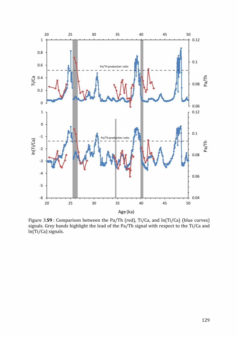
129

Figure 3.S9 : Comparison between the Pa/Th (red), Ti/Ca, and ln(Ti/Ca) (blue curves)

signals. Grey bands highlight the lead of the Pa/Th signal with respect to the Ti/Ca and

ln(Ti/Ca) signals.

0,04

0.06

0.08

0.1

0.12

-0,4

-0,2

0

0.2

0.4

0.6

0.8

1

20 25 30 35 40 45 50ln

(Ti/

Ca

)

Pa

/Th

Ti/

Ca

Pa

/Th



Age (ka)

0.04

0.06

0.08

0.1

0.12

-6

-5

-4

-3

-2

-1

0

1

20 25 30 35 40 45 50

130

Tables

Table 3.S1 : Age model for core GeoB3910.

14C dates are from ref. 2 except one date measured for this study (*)

** 14C dates that were not used and were replaced by speleothem tie points

*** speleothem tie points

14C_age (y BP) is the uncalibrated conventional radiocarbon age, age (Cal y BP) is the

calendar age obtained using the Marine13 calibration curve 18 or U‐Th dates (***), the

modeled age (Cal y BP) is the calendar age model produced by the Oxcal software 19.

Depth&(cm) &14C&age&(y&BP) ±&1σ Age&(Cal&y&BP) ±&1σ Modeled&Age&(Cal&y&BP) ±&1σ

0 565 30 202 56 190 74

13 3930 35 3910 54 3918 80

23 6160 40 6595 56 6586 72

38 8430 40 9033 52 9037 76

58 10090 60 11103 73 11072 94

73 10940 70 12500 99 12460 131

88 12840 110 14528 277 14610 352

103 13550 70 15793 127 15798 177

113 14000 70 16378 124 16374 164

148 15780 110 18650 114 18642 119

173 20000 170 23624 226 23441 256

183 20580 150 24243 183 24359 246

* 200 22850 130 26764 216 26779 272

213 25130 260 28763 286 28712 303

233 27160 310 30921 202 30947 129

238 28280 430 31742 493 31538 303

268 30860 430 34419 360 34511 293

*** 300 / 38350 713 38316 504

*** 324 / 39840 713 39839 504

** 328 38600 1480 42323 1220 /

** 348 41000 820 44114 707 /

** 373 44480 1250 47349 1269 /

*** 377 / 47060 721 47060 516

*** 400 / 48520 714 48493 506

131

Table 3.S2 : Age model for core MD09‐3257.

* 14C dates measured on core MD09‐3257

** speleothem tie points

Dates are otherwise based on the correlation with core GeoB3910.

Depth&GeoB3910&(cm) Depth&MD0933257&(cm) 14C&age&(y&BP) ±&1σ Modeled&Age&(Cal&y&BP) ±&1σ

* / 0 795 30 447 31

* / 40 6355 30 6823 49

* / 80 9985 35 10984 83

73 109 / 12425 130

100 135 / 15594 236

122 162 / 16914 228

145 183 / 18234 385

* / 227 20460 70 24120 115

* / 245 21870 80 25785 85

215 262 / 28972 371

225 273 / 30132 486

232 282 / 30879 158

251 301 / 32824 299

263 312 / 34060 295

284 330 / 36361 295

** / 347 / 38350 504

** / 371 / 39840 504

** / 422 / 47060 516

** / 440 / 48520 506

132

Table 3.S3 : 231Pa, 230Th, 232Th, and 238U concentrations (dpm.g‐1) versus depth in core

MD09‐3257. Pa/Th values are computed with a R ratio of 0.5.

Prof(cm) Age (y) 1 σ231

Pa 1 σ230

Th 1 σ232

Th 1 σ238

U 1 σ Pa/Th 1 σ

0 447 31 0.176 0.006 2.98 0.06 1.08 0.02 1.327 0.026 0.062 0.003

10 2041 35 0.219 0.012 3.49 0.06 1.10 0.02 1.390 0.013 0.067 0.004

200 20483 282 0.222 0.007 3.90 0.06 2.24 0.03 1.326 0.009 0.078 0.004

210 21830 220 0.153 0.004 2.79 0.06 2.02 0.04 1.540 0.030 0.076 0.004

213 22234 201 0.223 0.004 3.78 0.22 2.29 0.13 1.470 0.016 0.084 0.008

215 22504 189 0.207 0.004 3.86 0.09 2.58 0.05 1.490 0.013 0.075 0.003

218 22908 170 0.191 0.003 3.76 0.08 2.62 0.03 1.617 0.012 0.069 0.003

220 23177 158 0.178 0.005 3.63 0.09 2.72 0.06 1.683 0.040 0.066 0.004

220 23177 158 0.184 0.003 3.61 0.05 2.76 0.03 1.678 0.045 0.070 0.002

225 23851 127 0.169 0.003 3.28 0.05 3.13 0.04 1.675 0.016 0.075 0.004

227 24120 115 0.190 0.004 3.54 0.05 3.43 0.03 1.906 0.016 0.080 0.004

245 25785 85 0.294 0.006 4.43 0.07 2.92 0.04 2.187 0.033 0.104 0.004

245 25785 85 0.296 0.005 4.43 0.08 2.95 0.04 2.181 0.050 0.105 0.004

247 26151 117 0.252 0.004 4.02 0.07 3.13 0.04 2.061 0.015 0.100 0.004

250 26701 167 0.225 0.006 3.95 0.07 2.51 0.04 1.684 0.031 0.084 0.004

250 26701 167 0.220 0.004 3.96 0.08 2.50 0.04 1.685 0.014 0.081 0.003

252 27067 200 0.187 0.004 3.66 0.07 2.14 0.03 1.482 0.013 0.072 0.003

255 27617 249 0.173 0.004 3.39 0.06 2.38 0.03 1.469 0.013 0.074 0.004

257 27983 282 0.162 0.003 3.38 0.09 2.54 0.05 1.475 0.011 0.067 0.004

257 27983 282 0.159 0.003 3.36 0.07 2.55 0.03 1.467 0.010 0.066 0.003

260 28532 331 0.180 0.003 3.60 0.10 3.11 0.06 1.545 0.010 0.075 0.005

313 34213 295 0.155 0.003 3.06 0.08 2.53 0.05 1.522 0.013 0.080 0.005

315 34467 295 0.153 0.003 3.05 0.06 2.27 0.02 1.533 0.013 0.077 0.004

317 34721 295 0.140 0.003 2.86 0.07 2.08 0.04 1.402 0.014 0.074 0.004

320 35102 295 0.134 0.003 2.91 0.06 2.30 0.04 1.460 0.010 0.067 0.004

323 35484 295 0.137 0.003 2.93 0.07 2.46 0.05 1.375 0.008 0.071 0.004

325 35738 295 0.170 0.002 3.38 0.07 2.96 0.05 1.551 0.012 0.082 0.004

327 35992 295 0.165 0.002 3.24 0.05 2.91 0.03 1.517 0.019 0.084 0.004

330 36373 297 0.138 0.003 2.95 0.07 2.43 0.05 1.367 0.011 0.072 0.004

333 36722 333 0.142 0.003 2.74 0.04 1.77 0.02 1.534 0.012 0.080 0.004

335 36954 358 0.143 0.002 3.02 0.06 1.86 0.03 1.890 0.011 0.067 0.003

338 37303 394 0.130 0.002 2.66 0.05 1.78 0.02 1.634 0.015 0.072 0.003

338 37303 394 0.120 0.004 2.64 0.07 1.75 0.03 1.595 0.012 0.062 0.005

340 37536 419 0.137 0.003 2.94 0.06 2.23 0.03 1.726 0.013 0.068 0.004

341 37652 431 0.143 0.002 2.91 0.07 2.28 0.04 2.994 0.030 0.060 0.005342 37768 443 0.141 0.002 3.08 0.07 2.63 0.04 1.900 0.011 0.066 0.004

343 37885 455 0.145 0.003 2.98 0.06 2.73 0.04 1.742 0.022 0.077 0.005345 38117 480 0.155 0.002 3.13 0.06 2.83 0.05 1.737 0.012 0.080 0.004

347 38350 504 0.179 0.003 3.45 0.06 3.18 0.04 2.128 0.034 0.087 0.005

347 38350 504 0.158 0.004 3.39 0.06 3.09 0.04 2.072 0.026 0.070 0.005

350 38540 504 0.176 0.002 3.48 0.07 4.05 0.06 2.019 0.018 0.090 0.006

350 38540 504 0.176 0.003 3.52 0.06 4.03 0.04 2.021 0.011 0.088 0.005

352 38667 504 0.163 0.003 3.16 0.06 3.90 0.06 2.091 0.022 0.096 0.007354 38794 504 0.189 0.003 3.43 0.06 3.95 0.05 2.317 0.026 0.106 0.007

354 38794 504 0.177 0.004 3.42 0.06 3.84 0.05 2.295 0.017 0.091 0.007

360 39174 504 0.144 0.004 3.01 0.06 4.00 0.06 3.181 0.051 0.058 0.014370 39808 504 0.169 0.003 2.94 0.05 3.99 0.05 2.009 0.049 0.132 0.011

372 40052 504 0.161 0.002 3.04 0.07 2.75 0.05 2.422 0.046 0.087 0.006

374 40335 505 0.141 0.003 2.82 0.04 2.20 0.02 1.431 0.015 0.083 0.004

376 40619 505 0.138 0.002 2.77 0.06 1.93 0.03 1.763 0.031 0.077 0.004

378 40902 505 0.130 0.002 2.79 0.05 1.87 0.02 1.324 0.008 0.073 0.003

380 41185 506 0.117 0.002 2.48 0.06 1.79 0.04 1.185 0.008 0.075 0.004

382 41468 506 0.137 0.002 2.58 0.05 2.19 0.03 1.305 0.013 0.094 0.005

385 41893 507 0.133 0.003 2.76 0.05 2.56 0.04 1.410 0.009 0.081 0.005

387 42176 508 0.156 0.003 3.24 0.07 3.03 0.05 1.592 0.016 0.082 0.005

390 42601 508 0.148 0.003 3.19 0.09 2.68 0.03 1.474 0.009 0.076 0.005

133

Table 3.S4 : Cibicides wuellerstorfi δ13C values versus depth in core GeoB3910.

Depth&(cm) Age&(ka) δ13C&(‰) Depth&(cm) Age&(ka) δ13C&(‰) Depth&(cm) Age&(ka) δ13C&(‰) Depth&(cm) Age&(ka) δ13C&(‰)

59.5 11211 80.13 219.5 29544 0.76 290 37095 1.14 367 45737 1.2

65 11720 0.37 221.5 29800 0.3 291 37212 1.09 368 45875 1.23

69 12090 0.46 223.5 30012 0.42 292 37329 1.16 370 46150 1.17

72 12367 0.44 228 30455 0.61 293 37447 1.13 372 46426 1.11

73 12460 0.4 231 30750 0.74 294 37564 1.15 373 46564 1.17

76 12901 0.27 232.5 30898 0.73 295 37682 1.17 375 46839 0.63

83 13898 0.74 234.5 31134 0.74 296 37799 1.11 379 47208 0.52

90 14875 0.03 236 31307 0.79 297.5 37975 0.97 385 47579 0.49

91.5 15073 0.14 237.5 31480 0.64 302.7 38463 0.34 387 47702 0.42

94 15259 0.08 239.5 31687 0.61 311.5 39026 0.41 390 47888 0.39

96 15379 80.09 241 31835 0.47 318 39442 0.71 393 48073 0.49

99.5 15588 0.22 242 31934 0.89 319 39506 0.58 396 48258 0.63

105 15913 0.23 243 32033 0.98 320.5 39602 0.45 397 48320 0.58

108 16086 0.07 244 32133 0.7 322.5 39730 0.57 400 48499 0.74

111 16259 0.05 246 32331 0.8 324.5 39880 0.79 401 48529 0.89

114 16431 0.11 247 32430 0.93 326 40087 0.75 402 48560 0.89

118 16660 0.17 248 32529 0.82 327 40225 0.95 407 48712 1.06

127 17177 0.14 249.5 32678 0.7 328 40363 0.79 415 48957 1.2

134.5 17607 0.24 250 32727 0.94 329.5 40569 0.85 416 48987 1.18

138.5 17836 0.29 251.5 32876 0.5 332 40914 0.89 417 49018 1.09

144.5 18181 0.61 252 32925 0.61 333 41052 0.89 419 49079 1.19

146 18310 0.57 253 33024 0.81 334 41189 1.07 421 49140 1.16

148 18642 0.66 254 33123 0.7 335 41327 1.03 423 49201 1.11

150 19026 0.69 255 33223 0.93 336 41465 1.02 424 49231 1.17

153.5 19697 0.62 256 33322 0.74 337 41603 1.05 425 49262 1.1

157 20369 0.77 257 33421 0.79 338.5 41809 0.83 426 49292 1.2

160 20945 0.66 258 33520 0.85 340 42016 0.78 427 49323 1.16

162.5 21425 0.65 258.5 33569 1.01 341 42154 0.87 430 49414 1.14

169 22673 0.59 262 33916 0.85 342 42292 0.92 432 49475 1.15

173 23441 0.82 264 34114 0.75 343 42429 0.91 433 49506 1.15

176 23717 0.56 265 34213 0.81 344 42567 1.07 441 49750 0.72

177.5 23855 0.85 266 34313 0.85 346 42843 1.03 451 50055 0.75

179 23994 0.48 267 34412 0.97 347 42981 1.19 452 50085 0.78

184 24497 0.71 268 34511 1.06 349 43256 1.18 453 50116 0.94

188.5 25117 0.37 269 34628 1.11 350 43394 1.12 454 50146 1

193.5 25805 0.49 270 34746 1.13 351 43532 1.03 456 50207 0.91

199 26628 0.67 271 34863 1.12 352 43669 1.12 458 50268 0.83

204 27374 0.92 272 34981 1.05 353 43807 0.68 459 50299 0.92

205 27523 0.78 273 35098 1.19 354 43945 0.76 460 50329 0.93

206 27672 0.55 274 35215 0.77 355 44083 1.07 461 50360 0.95

207 27820 0.74 276.5 35509 0.76 356 44221 0.79 463 50421 0.84

208.5 28043 0.91 278.5 35744 0.97 357 44359 0.76 464 50451 0.88

210 28266 0.57 280 35920 1.02 358 44496 1.13 466 50512 0.55

211 28415 0.91 281 36038 0.85 359 44634 1.04 468 50573 0.3

212 28564 0.98 282 36155 0.83 360 44772 1.04 471 50664 80.14

213 28712 0.72 283 36272 0.92 361 44910 1.16 472 50741 0.14

214 28840 0.76 284 36390 0.88 362 45048 1.08 476 51169 80.11

215 28968 0.93 285 36507 0.98 363 45186 0.94 481 51705 80.17

216 29096 1.16 286 36625 0.86 364 45323 1.13 482 51812 80.56

217 29224 0.8 288 36860 1.12 365 45461 1.24 484 52026 80.2

218 29352 0.79 289 36977 1.12 366 45599 1.18 501 53847 0.02

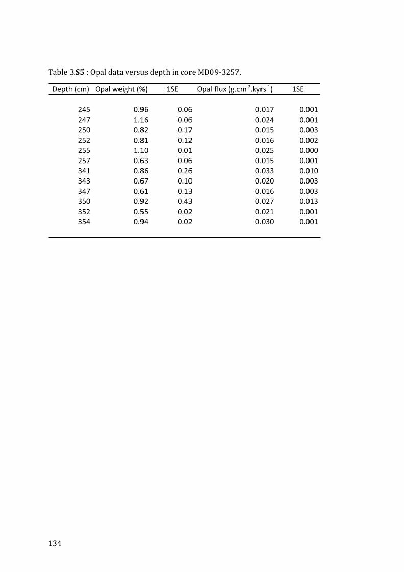
134

Table 3.S5 : Opal data versus depth in core MD09‐3257.

Depth&(cm) Opal&weight&(%) 1SE Opal&flux&(g.cm92.kyrs91) 1SE

245 0.96 0.06 0.017 0.001

247 1.16 0.06 0.024 0.001

250 0.82 0.17 0.015 0.003

252 0.81 0.12 0.016 0.002

255 1.10 0.01 0.025 0.000

257 0.63 0.06 0.015 0.001

341 0.86 0.26 0.033 0.010

343 0.67 0.10 0.020 0.003

347 0.61 0.13 0.016 0.003

350 0.92 0.43 0.027 0.013

352 0.55 0.02 0.021 0.001

354 0.94 0.02 0.030 0.001

135

3.4 Additional elements of discussion

In this chapter, I interpreted the increase in Pa/Th ratio and decrease in benthic δ13C

preceding southward ITCZ shifts as a reduction in the intensity of the AMOC upper

circulation cell. However, one could argue that such a Pa/Th and δ13C variation could

also result from a shoaling of the northern‐sourced water mass, giving way to a

southern‐sourced water mass at 2300 m depth. Because such a circulation scheme

would also imply a reduction of the AMOC upper circulation cell intensity my

conclusions remain valid. Note that a more complete discussion of the possible structure

of the AMOC during Heinrich Stadials is provided in chapter 4.

The data I present in chapter 3 indicates that large slowdowns of the AMOC upper

circulation cell took place before the onset of Heinrich Stadials. These results are in

contradiction with a recent study of Lynch‐Stieglitz et al. (2014), in which the strength

of the Florida Current is assessed during HS1‐HS3 based on the horizontal density

gradient across the Florida Strait, inferred from the benthic δ18O horizontal gradient at

~550 m depth. This study concluded that the strength of this current, and hence of the

AMOC upper circulation cell, did not vary during HS2 and HS3. However, one of the

cores used to assess the benthic δ18O horizontal gradient has a very low sedimentation

rate and was measured at low resolution, so that there is only one data point during HS2

and HS3. A slowdown of the AMOC upper circulation cell could thus likely be missed in

their record, while our Pa/Th and benthic δ13C records clearly show that Heinrich

Stadial 2 is associated with a substantial AMOC slowdown.

137

Chapter 4: Changes in the geometry and strength of the AMOC

during the last glacial

4.1 Introduction

In chapter 3, I used the sedimentary Pa/Th ratio measured in the equatorial sediment

core of intermediate depth to infer changes in the renewal rate of the overlying water

mass during the last glacial. I interpreted the sedimentary Pa/Th increase preceding the

precipitation events as a decreased renewal rate of the northern‐sourced intermediate

water mass, and hence likely of the upper circulation cell of the AMOC. Indeed, a

slowdown of the intermediate water mass could increase the sedimentary Pa/Th ratio

by decreasing the export of dissolved protactinium. However, the replacement of the

northern sourced water mass by a southern sourced water mass could cause a similar

Pa/Th increase and δ13C decrease in the intermediate core. Nonetheless, replacing the

northern sourced water mass by a southern sourced water mass could also reflect a

reduction of the upper circulation cell of the AMOC, so that the conclusions of the study

would remain unchanged. Using one sediment core it was possible to assess the timing

of the AMOC change with respect to the ITCZ shift but not to infer changes in the

strength and geometry of the AMOC.

In order to address this issue, the sedimentary Pa/Th ratio needs to be analyzed in cores

recovered from different depths and latitudes. Indeed, sedimentary Pa/Th equilibrates

with the water masses occupying the first 1000 m above the seafloor (Thomas et al.,

2006). Hence, previous studies used sediment cores recovered from a vertical transect

on the northern Brazilian margin or from all over the Atlantic Ocean to reconstruct the

strength and geometry of the AMOC at present (Lippold et al., 2011) and during the LGM

(Lippold et al., 2012a).

In an ideal ocean affected by a single uniform water mass, the deviation of total

protactinium and thorium concentrations from linear increase with depth at a study site

is solely dependent on the water mass transfer time from the region of deep‐water mass

formation to the study site. At present, because the vertical extent of NADW is large

(1200–4000 m depth at the equator, (Schott, 2003)), estimating the flow rate of NADW

based on total protactinium and thorium concentrations is therefore possible using a

simple equation (Moran et al., 2002).

However, reconstructing a more complex vertical layout of water masses of different

strengths and origins based on sedimentary Pa/Th measurements is not possible using a

138

simple equation and requires the use of a Pa/Th model (Luo et al., 2010; Siddall et al.,

2005).

To reconstruct the strength and geometry of the AMOC during the last glacial, I

measured the sedimentary Pa/Th ratio in the deep equatorial sediment core (MD09‐

3256Q, 3537 m) over two time intervals encompassing HS2 and HS4. Along with the

intermediate equatorial sediment core and with two other cores from the Bermuda Rise

(Lippold et al., 2009) and from the Cape Basin (Negre et al., 2010), I study the glacial

Pa/Th data of four sediment cores spanning different depths and latitudes. I compare

these data to simulated Pa/Th values obtained by forcing a simple 2D Pa/Th box model

with various streamfunctions (Luo et al., 2010). Streamfunctions were generated with

the iLOVECLIM model under different climatic conditions (Roche et al., 2014, in press).

By combining Pa/Th and δ13C data, I can infer the most likely state of the AMOC during

Heinrich Stadials and Dansgaard‐Oeschger interstadials.

I use the δ13C of the deep equatorial core (3537 m depth) in order to evaluate the

influence of southern sourced water masses at the core site during the last glacial.

However, a decreased δ13C in the deep core can be interpreted as an increased influence

of southern‐ compared to northern‐sourced waters, or as a change in the δ13C end

member of the water mass affecting the core. I therefore investigated published C.

wuellerstorfi δ13C records of sediment cores below 4000‐4500 m depth close to the

study area. Indeed, δ13C variations of similar amplitude in deep and abyssal cores could

be interpreted as variations in the δ13C end member of the water mass affecting the

cores. However, no sediment cores were analyzed for δ13C below 4000‐4500 m in my

study area, apart for a few whose age model is not robust enough. Hence, I cannot

disentangle changes in δ13C end members from changes in water masses, and therefore

interpret decreases in the δ13C records as increased influence of southern sourced

waters.

Results of the Pa/Th data‐model comparison are detailed in section 4.2, within the

article entitled “Changes in the geometry and strength of the AMOC during the last

glacial”. I find that interstadials of the last glacial were likely characterized by a

northern‐sourced circulation cell active above ~2500 m depth, and by a southern‐

sourced circulation cell active below. The strength of the northern sourced water mass

was likely lower than present day NADW and the strength of the southern sourced

water mass could have been similar to present day AABW. At the onset of Heinrich

Stadials, the geometry of the AMOC changed significantly. More specifically, my data

suggest that at the onset of HS2, the Atlantic Ocean was dominated by southern sourced

waters below 1300 m depth.

139

4.2 Changes in the geometry and strength of the AMOC during the last

glacial

This article has not been sent to all co‐authors for an internal review yet, and minor

changes are expected before submission.

140

Changes in the geometry and strength of the AMOC during the last glacial

Pierre Burckela, Claire Waelbroecka, Yiming Luob, Didier Rochea, Sylvain Pichatc, Jeanne

Gherardia, Aline Govind, François Thila

aLSCE/IPSL, Laboratoire CNRS‐CEA‐UVSQ, Bât.12, avenue de la Terrasse, F‐91198 Gif

sur Yvette, France

bDalhousie University, Department of Oceanography, 1355 Oxford Street, PO BOX

15000, Halifax, NS B3H 4J1, Canada

cLaboratoire de Géologie de Lyon (LGL‐TPE), Ecole Normale Supérieure de Lyon, 46


dMARUM – Center for Marine Environmental Sciences, University of Bremen, Bremen,

Germany

*Corresponding author: [email protected] +33 (0)1.69.82.43.47

141

Abstract

We study last glacial sedimentary Pa/Th in sediment cores recovered from various

depths and latitude in the Atlantic Ocean. We compare these data to Pa/Th values

simulated with a simple 2D box model forced with streamfunctions generated under

different climatic conditions. This allows us to reconstruct the geometry and strength of

the AMOC during interstadials of the 20‐50 ka period. We show that circulation during

interstadials was very different from that of the Holocene. Northern sourced waters

were likely circulating above 2500 m depth, with a flow rate lower than that of the

present day North Atlantic Deep Water (NADW). Southern sourced deep waters flowed

northwards below 4000 m depth, and southwards as a return flow between 2500 and

4000 m depth. The flow rate of this southern sourced deep water could have been

equivalent to that of the modern Antarctic Botton Water (AABW). At the onset of

Heinrich Stadials, the structure of the AMOC significantly changed. The Atlantic Ocean

was probably directly affected by a southern sourced water mass below 2500 m depth,

while sluggish waters influenced depths between 1300 and 2300 m.

Introduction

Temperature variability recorded in Greenland ice cores shows that the last glacial

climate repeatedly shifted between cold (stadial) and warm (interstadial) conditions

(Johnsen et al., 1992), the so‐called D‐O cycles (Dansgaard et al., 1993). Greenland

stadials typically lasted several centuries, and were followed by a rapid warming of up

to 15°C achieved within a few decades (Kindler et al., 2014). Interstadial conditions then

lasted several centuries, with Greenland temperatures slowly decreasing and leading to

the onset of a new stadial. During some of the stadials, icebergs were released from the

Laurentide ice sheet into the North Atlantic Ocean, depositing ice rafted detritus into

marine sediment cores (Heinrich, 1988). We refer to these periods as Heinrich Stadials

(HS).

Changes in Atlantic oceanic circulation have long been suggested to impact Greenland

temperatures (Broecker et al., 1985) and could be at the origin of the DO variability.

Indeed, there are numerous evidences of decreased North Atlantic deep water formation

and increased influenced of southern sourced deep waters in the Atlantic Ocean during

Heinrich Stadials (Elliot et al., 2002; Robinson and van de Flierdt, 2009; Vidal et al.,

1997). Moreover, climate models are able to reproduce the characteristic patterns of the

Dansgaard‐Oeschger variability through variations of the strength of the Atlantic

Meridional Overturning Circulation (AMOC) (Stocker and Johnsen, 2003). However,

recent studies show that a shallow circulation cell could have been still active during

Heinrich Stadials (Gherardi et al., 2009; Lynch‐Stieglitz et al., 2014), meaning that other

mechanisms could be required to explain Greenland temperature variability. Further

142

understanding the vertical layout and flow rate of the water masses constituting the

AMOC during the last glacial is therefore required before assessing the relationship

between AMOC and DO variability.

Sedimentary (231Pa/230Th)xs,0 (activity ratio of 231Pa and 230Th unsupported by lithogenic

and authigenic uranium and corrected from decay to the time of sediment deposition,

Pa/Th hereafter)(Yu et al., 1996) has been used in the Atlantic to infer changes in

oceanic circulation intensity during Heinrich Stadials (Gherardi et al., 2005; Gherardi et

al., 2009; McManus et al., 2004; Yu et al., 1996) (Burckel et al., in prep). Although a

recent study questions the ability of dissolved Pa/Th to reflect the flow rate of water

masses in the south Atlantic (Deng et al., 2014), several studies comparing simulated

sedimentary Pa/Th values to core top Pa/Th data have shown that sedimentary Pa/Th

reflects circulation intensity in the modern Atlantic Ocean (Lippold et al., 2011; Siddall

et al., 2005).

However, interpretation of sedimentary Pa/Th on a single sediment core might be

complicated by the non‐linear response of Pa/Th to circulation intensity changes (Luo et

al., 2010). Reconstructing present and past strength of the AMOC is therefore best

achieved by studying sediment cores at different depths and latitudes (Gherardi et al.,

2009; Lippold et al., 2011; Lippold et al., 2012).

In this study, we present new sedimentary Pa/Th data from a deep sediment core

retrieved off the Brazilian margin. We compare last glacial Pa/Th values of sediment

cores from different depths and latitudes to Pa/Th values simulated using a simple 2D

box model (Luo et al., 2010) forced by various streamfunctions. The streamfunctions

were simulated with the Earth System model iLOVECLIM under different climatic

conditions (Roche et al., 2014, in press). Results from this comparison allow us to

constrain the geometry and strength of the AMOC during DO interstadials and Heinrich

Stadials.

Study area

Sediment cores MD09‐3257 (04°14.69’S, 36°21.18’W, 2344m water depth) and MD09‐

3256Q (03°32.81’S, 35°23.11’W, 3537m water depth) were recovered from the Brazilian

margin during R/V Marion Dufresne cruise MD173/RETRO3 (Fig. 1). Core GeoB3910

(04°14.7’S, 36°20.7’W, 2362m water depth) (Jaeschke et al., 2007) was recovered at

approximately the same position and depth as core MD09‐3257, during Meteor cruise

M34/4. We therefore refer to both GeoB3910 and MD09‐3257 as intermediate

equatorial cores, and to MD09‐3256Q as the deep equatorial core. At present, the water

mass influencing the Brazilian margin at these depths is the southward flowing North

Atlantic Deep Water (NADW), a water mass originating from the Nordic seas and

influencing most of the deep Atlantic Ocean (Fig. 1). Because the Brazilian margin is

143

affected by western boundary currents (Rhein et al., 1995), these sediment cores are

ideally located to observe changes in the strength and extent of the intermediate and

deep AMOC water masses (Schott, 2003).

We compare our Pa/Th data with published records from other Atlantic cores: ODP Leg

172 site 1063 (33°41’N, 57°37’W, 4584 m) (Lippold et al., 2009) and MD02‐2594

(34°43’S, 17°20’E, 2440 m) (Negre et al., 2010) (Fig. 1).

Material and method

Benthic δ13C

δ13C (13C/12C isotopic ratio) of the epifaunal benthic foraminifer Cibicides wuellerstorfi

has been shown to record the δ13C of bottom water dissolved inorganic carbon (DIC)

with minor isotopic fractionation (Duplessy et al., 1984; Zahn et al., 1986). Initial DIC

carbon isotopic concentration is acquired by a water mass in its formation region by

surface productivity, which consumes 12C therefore increasing dissolved δ13C, and

temperature dependent air‐sea interactions (Lynch‐Stieglitz et al., 1995; Rohling and

Cooke, 1999). The δ13C of the DIC then evolves as deep‐water ages, because of the

constant export of 12C enriched biogenic material remineralized at depth, which

decreases the DIC δ13C along the flow path of the water mass. As DIC δ13C largely follows

water mass structure and circulation in the modern ocean, Cibicides δ13C has been used

to trace water masses, a decrease in Cibicides δ13C being interpreted as a decrease in

bottom water ventilation, and conversely (Duplessy et al., 1988). However, the

information on bottom water ventilation embedded in Cibicides δ13C is complicated by

the impact of changes in surface water δ13C and marine biological productivity.

Holocene and last glacial end member δ13C values are systematically higher in northern

sourced waters (1.1 and 1.5 ‰ respectively) than in southern sourced waters (0.3 and ‐

0.2 ‰ respectively) (Curry et al., 1988; Curry and Oppo, 2005). Because the modern

variability of DIC δ13C largely follows the structure of water masses in the Atlantic Ocean

(Kroopnick, 1985), we interpret a decrease in the δ13C values as an increased influence

of nutrient‐rich southern sourced deep waters.

Core MD09‐3256Q benthic foraminifer C. wuellerstorfi were handpicked (>250µm

fraction), washed with methanol in an ultrasonic bath then roasted in glass vials at

380°C under vacuum for 45 min. C. wuellerstorfi δ13C (expressed in ‰ VPDB) were

measured at LSCE (Gif‐sur‐Yvette) using an Elementar Isoprime mass spectrometer.

VPDB is defined with respect to NBS‐19 calcite standard (δ18O = ‐2.20 ‰ and δ13C =

+1.95 ‰) (Coplen, 1988). The mean external reproducibility (1σ) of carbonate

144

standards is ± 0.05 ‰ for δ18O and ± 0.03 ‰ for δ13C; measured NBS‐18 δ18O is ‐23.2 ±

0.2 ‰ VPDB and δ13C is ‐5.0 ± 0.1 ‰ VPDB. δ13C measurements were done at the

highest possible resolution, depending on the availability of C. wuellerstorfi (generally

every 1 to 2 cm).

Sedimentary Pa/Th

In contrast to C. wuellerstorfi δ13C, which reflects the nutrient content of water masses,

sedimentary Pa/Th is a relatively recent proxy that records the renewal rate of water

masses occupying the first 1000 m above the seafloor (Thomas et al., 2006). Hence, the

proxy has been successfully used as a tracer of oceanic circulation intensity in the

Atlantic Ocean (Gherardi et al., 2005; Gherardi et al., 2009; McManus et al., 2004).

231Pa and 230Th are produced at a constant Pa/Th activity ratio of 0.093 by dissolved

uranium, which is homogeneously distributed in the oceans. 230Th is however much

more particle reactive than 231Pa, as reflected by their respective residence time in the

ocean (30‐40 y for 230Th, 200 y for 231Pa (Francois, 2007)). 230Th is therefore rapidly

removed to the underlying sediment, while 231Pa can be laterally exported by oceanic

currents. High flow rates therefore result in high 231Pa export and low sedimentary

Pa/Th ratio, and conversely. However, affinities of 231Pa and 230Th for settling particles

depend on the particle type (Chase et al., 2002). For instance, 231Pa has a high affinity for

opal, so that high opal fluxes can result in a high sedimentary Pa/Th ratio. The origin of

sedimentary Pa/Th variability therefore needs to be carefully assessed.

Pa/Th measurements were performed by isotopic dilution mass spectrometry on a

Thermo finnigan MC‐ICP‐MS Neptune, following the method of Guihou et al., 2010. Pa

and Th are decay corrected to the time of sediment deposition and from the lithogenic

component by using a 238U/232Th ratio of 0.5±0.1 (Fig. S1) (Guihou et al., 2010)(Burckel

et al., 2014 a, in prep.).

Age model

For the period between 0‐27 ka, core MD09‐3256Q age model is based on 6 14C dates

measured on planktic foraminifer G. ruber white and converted to calendar age using the

Marine13 curve (Reimer et al., 2013) (Fig. S2). During the last glacial, Heinrich Stadials

were recorded in marine sediment cores from the Brazilian margin as Ti/Ca peaks,

related to the increased terrigenous input associated with the southward shifts of the

ITCZ (Jaeschke et al., 2007). Ti/Ca peaks are therefore good stratigraphic markers for

correlating sediment cores with neighboring well‐dated cores. Therefore, from 27 ka to

50 ka, core MD09‐3256Q was dated by correlation of its Ti/Ca signal with that of core

GeoB3910 using 3 tie points corresponding to the Ti/Ca peaks associated with HS3‐5.

Resulting sedimentation rates are shown in Fig. S3. The age model is given in Table S1.

145

Circulation and Pa/Th model

The Pa/Th data of the studied sediment cores were compared to Pa/Th values simulated

using a simple 2D box model forced by different streamfunctions, in order to assess the

vertical layout and renewal rate of the water masses constituting the AMOC of the last

glacial. Streamfunctions were generated using the iLOVECLIM coupled climate model,

with atmosphere (ECBilt), ocean (CLIO) and vegetation (VECODE) components (Roche

et al., 2014, in press). A Last Glacial Maximum equilibrium state, computed using the

PMIP‐2 protocol, was used as background climate (see (Roche et al., 2007) for more

details). Streamfunctions corresponding to Heinrich Stadial 1 (HS1) and to a complete

shutdown of the AMOC (off‐mode) were generated by imposing a 0.16 and 0.35 Sv

freshwater forcing in the Labrador Sea (Roche et al., 2010) (Roche et al., 2014, in press),

respectively. Freshwater forcing was maintained for 300 y, and the streamfunction

generated 300 y after the end of the forcing. A freshwater input of 0.16 Sv allows the

presence of a shallow circulation cell in the Atlantic Ocean, while at 0.35 Sv the AMOC is

almost completely shutdown.

Pa/Th values were simulated along a meridional section in the Atlantic Ocean by forcing

a simple 2D box model (Luo et al., 2010) with the aforementioned streamfunctions (Fig.

2). Holocene simulated Pa/Th values and streamfunction are described in Lippold et al.,

2012 and Luo et al., 2010.

Dissolved Pa and Th concentrations in the model are controlled by (1) production from

U decay in the water column, (2) adsorption and desorption on settling particles and (3)

advection by oceanic circulation. Particulate Pa and Th concentrations are controlled by

(1) adsorption and desorption from the dissolved pool and (2) by removal of

sedimentary particles to the seafloor.

Modeled Pa/Th meridional sections generated with the different streamfunctions are

shown in Figure 2. Different water mass configurations can generate sedimentary Pa/Th

variations in the model (Luo et al., 2010). Increasing circulation intensity above a

specific location will cause Pa/Th to decrease at that depth because of the increased Pa

export and conversely. Increasing depth without modifying circulation intensity also

causes the sedimentary Pa/Th ratio to decrease in the model because of the increased

residence time of Pa with respect to scavenging and conversely. Finally, the sedimentary

Pa/Th ratio increases along the flow path of any water mass as the low dissolved Pa

concentrations of newly formed water masses increase by desorption of Pa from Pa‐

concentrated settling particles equilibrating with ambient waters (Francois, 2007).

Adsorption and desorption rate constants also impact the simulated Pa/Th ratio. These

constants were adjusted to reflect the opal belt in the southern ocean for all Pa/Th

146

simulations (Luo et al., 2010). For the Holocene, these constants were also changed to

reflect opal in the northern North Atlantic (Lippold et al., 2012).

Results

Sedimentary Pa/Th data

Core MD09‐3257 and MD09‐3256Q Pa/Th measurements were focused on HS2 and HS4

(Fig. 3, a). No Pa/Th values were measured within HS2 in core MD09‐3257 because of

the presence of turbidite layers (Burckel et al., 2014 b, in prep). During HS4 and before

HS2, the sedimentary Pa/Th ratio of core MD09‐3257 rises above the production ratio of

0.093, indicating the absence of protactinium export. Pa/Th variability associated with

DO stadials and interstadials is also observed, with high Pa/Th values occurring during

stadials and low values during interstadials. Pa/Th variations in core MD09‐3256Q are

more muted, so that the Pa/Th signal of core MD09‐3257 drives the Pa/Th difference

between the two cores. The main Pa/Th variation in core MD09‐3256Q occurs during

HS4, when Pa/Th values rise from ~0.06 to ~0.08.

Before interpreting our Pa/Th signals in terms of oceanic circulation, we need to assess

if varying lithogenic or opal fluxes impacted the scavenging intensities of Pa and Th. To

do so, we use the preserved opal and 232Th fluxes as proxies of past opal and terrigenous

fluxes respectively (Anderson et al., 2006; Lippold et al., 2012). Core MD09‐3257 Pa/Th

data are mainly influenced by oceanic circulation, except during the high lithogenic flux

period associated with HS4 (Fig. 3, a, white squares) (Burckel et al., 2014 b, in prep). In

core MD09‐3256Q, opal fluxes do not covary with the Pa/Th ratio and are very low

(0.01‐0.025 g.cm‐2.kyr‐1) (Fig. S4). In the Atlantic Ocean, the lower opal flux limit

observed to impact the sedimentary Pa/Th ratio is 0.2 g.cm‐2.kyr‐1 (Lippold et al., 2012).

Hence, given the much lower opal fluxes recorded in core MD09‐3256Q and their lack of

correlation with sedimentary Pa/Th, we conclude that biogenic silica had a minor

influence if any on the Pa/Th variability. In contrast, 232Th fluxes seem to correlate with

the Pa/Th ratio (P value = 0.0003, n = 20) (Fig. S5). This relation appears to be driven by

the high Pa/Th values occurring during the period of increased terrigenous fluxes

associated with HS4. Not considering these values, the Pa/Th appears to vary

independently from the terrigenous fluxes (P value = 0.79, n = 15). As such, we can

unfortunately not determine if the Pa/Th increase during HS4 is associated with a flow

rate decrease of the water mass above the sediment core. Increased Pa/Th could indeed

be due to the higher lithogenic fluxes that would enhance Pa scavenging and increase

the sedimentary Pa/Th ratio. Given the uncertainty on the cause of the Pa/Th rise, we

present the Pa/Th data within HS4 with different symbols (Fig. 3). Besides the period of

high terrigenous fluxes characterizing HS4, we can safely assume that the Pa/Th

147

variability recorded in our equatorial cores is mainly driven by changes in the flow rate

of the water masses occupying the bottom 1000 m at our core sites.

C. wuellerstorfi δ13C data

The Holocene δ13C value of the deep equatorial core was measured at 1.37 ‰, which is

assumed to be the modern δ13C value of NADW at our sites. No C. wuellerstorfi could be

found during the late Holocene in the intermediate core.

δ13C values of the last glacial are lower than during the Holocene (Fig. 3), which could

indicate a general increased influence of southern sourced water masses on both

intermediate and deep sediment cores. It could also reflect the less developed

continental biosphere associated with glacial periods (Duplessy et al., 1988).

δ13C values in the deep core are systematically lower than values in the intermediate

core. This could reflect an increased influence of the deep southern sourced water mass

with depth. δ13C of both cores shows millennial scale variability, with low δ13C values

occurring during Heinrich Stadials. DO stadials and interstadials are also recorded in the

δ13C record of the intermediate core by low and high δ13C values respectively. In the

deep core, the low sedimentation rate could have smoothed out the δ13C decrease

associated with the short DO stadials.

Time slice definition

We define 4 time slices to compare the Pa/Th data of the Brazilian margin and Bermuda

Rise cores to Pa/Th values simulated with the different streamfunctions (Fig. 3). We do

not study core MD02‐2594 within the time slices, as Pa/Th during the 20‐50 ka period is

measured at low resolution in the core (Fig. S6).

Pre‐HS2, Post‐HS4 and Pre‐HS4 time slices are defined as the periods of low equatorial

sedimentary Pa/Th values preceding (Pre‐) or following (Post‐) Heinrich Stadials 2 and

4 (Fig. 3). Pa/Th data are considered low when they equal the minimum Pa/Th value

preceding or following the Heinrich Stadial of interest within 1‐sigma uncertainties. For

Pre‐HS2, low Pa/Th values were defined in core MD09‐3257, as the Pa/Th signal of core

MD09‐3256Q presents no variability within 1‐sigma uncertainties across the transition

towards Heinrich Stadial 2.

We consider that these time slices represent interstadial conditions. Indeed, the Post‐

HS4 time slice corresponds to DO8, and is characterized by low Pa/Th values, high δ13C

values and high Greenland temperatures (Fig. 3). Pre‐HS4 encompasses both DO10 and

the short stadial between DO9 and DO10. However, given dating uncertainties as well as

the high δ13C and low Pa/Th at that time in the equatorial core of intermediate depth, we

conclude that Pre‐HS4 probably recorded interstadial conditions. Pre‐HS2 recorded DO3

as well as the two stadials preceeding and following DO3. Given dating uncertainties and

148

the high δ13C and low Pa/Th of both equatorial cores at that time, we consider that the

Pre‐HS2 time slice reflects interstadial conditions.

The HS2 time slice was defined in core MD09‐3257 during the period of decreased

sedimentary Pa/Th variation with time after the abrupt rise associated with the onset of

HS2.

The HS2 time slice probably corresponds to the stadial conditions associated with

Heinrich Stadial 2. Indeed, at that time, Pa/Th data of core MD09‐3257 are already

above the production ratio, Pa/Th data at ODP site 1063 reached their stadial values and

Pa/Th data in core MD09‐3256Q are similar before and during HS2. Moreover, the δ13C

of both equatorial cores nearly reached their low δ13C values associated with HS2.

Sedimentary Pa/Th values associated to each time slice and cores are given in Table S2.

Discussion

Interstadials

Pa/Th data from the Brazilian margin and Bermuda Rise cores are compared, when

available, to the Pa/Th model forced by the different streamfunctions (Fig. 4‐6). We

often describe the modeled and measured sedimentary Pa/Th of the equatorial cores by

referring to the vertical Pa/Th gradient between 2300 and 3500 m (i.e. the depths of the

sediment cores). Indeed, vertical Pa/Th gradients are useful indicators of the vertical

layout of water masses. A large gradient indicates that the Pa/Th of the deep core is

significantly lower than the Pa/Th of the intermediate core. A small gradient indicates

that sedimentary Pa/Th values of both cores are similar. In what follows, we will see

how each vertical gradient can be interpreted.

A large vertical Pa/Th gradient between the two equatorial core sites is simulated by the

model in the presence of a southward flowing northern‐sourced deep water mass such

as NADW in the Holocene simulation (Fig. 4). This is due to the fact that within a single

water mass of uniform flow rate, the sedimentary Pa/Th ratio decreases with depth.

This effect is intensified in the case of the Holocene streamfunction, as the flow rate of

NADW is not uniform but stronger between 2500‐3500 m and weaker between 1300‐

2300 m (depths of acquisition of sedimentary Pa/Th for the deep and intermediate

cores respectively). Hence, Pa export at 3500 m is more intense than at 2300 m,

therefore significantly increasing the vertical Pa/Th gradient between the two cores.

Interstadial Pa/Th data in the deep equatorial and Bermuda Rise cores are consistent

with simulated Pa/Th values obtained with the Holocene streamfunction (Fig. 4, b‐d).

However, interstadial sedimentary Pa/Th values in the equatorial core at intermediate

depth are lower than predicted by the Pa/Th model forced with the Holocene

streamfunction. The vertical Pa/Th gradient between our equatorial cores is therefore

small, which is in contradiction with the large vertical Pa/Th gradient generated by the

149

Holocene streamfunction. Moreover, data from Southern Ocean core MD02‐2594 are

systematically below 0.06 during the last glacial (Fig. S6), and are in conflict with the

high simulated Holocene Pa/Th value (~0.09) at 34°S and ~2400 m depth.

High δ13C values in the intermediate equatorial core during MIS3 interstadials suggest

that northern‐sourced deep waters influenced the equatorial Atlantic at 2300 m depth

(Fig. 3, b). However, the lower δ13C values of the deep equatorial core imply that, unlike

in the present day Atlantic Ocean, nutrient rich southern sourced deep waters were

influent at 3500 m depth.

Therefore, both Pa/Th and δ13C data indicate that the geometry and strength of the

AMOC during interstadials was different from that of the Holocene.

Pa/Th values simulated with the off‐mode streamfunction exhibit a small vertical Pa/Th

gradient between the two equatorial cores (Fig. 5). However, measured sedimentary

Pa/Th during interstadials are much lower than the simulated values at both equatorial

sites. Low measured Pa/Th values imply a significant export of Pa by oceanic circulation

and therefore exclude the possibility of an almost halted oceanic circulation above 2300

and 3500 m depth (Fig. 5, b‐d).

In the off‐mode streamfunction, no deep convection occurs in the high latitude North

Atlantic. However, the high δ13C values of the intermediate equatorial core indicate that

northern sourced waters were influent at 2300 m.

Hence, it is highly unlikely that the off‐mode streamfunction depicts the Atlantic Oceanic

circulation during interstadials of the last glacial.

The HS1 streamfunction also generates a small vertical Pa/Th gradient between our

equatorial cores (Fig. 6). In contrast to the simulation obtained with the off‐mode

streamfunction, this small vertical Pa/Th gradient is associated with significant lateral

export of Pa at the depth of both the intermediate and deep equatorial cores, as well as

at the Bermuda Rise and Southern Ocean cores, consistently with Pa/Th data (Fig. 6, b‐

d). Such a small vertical Pa/Th gradient is simulated in the case of two water masses

overlying each other and flowing in opposite directions (Fig. S7) (Lippold et al., 2012).

This circulation scheme results in decreasing or invariant lateral export of Pa with

depth, which in turns causes sedimentary Pa/Th to increase or to be constant with

depth.

Interstadial benthic δ13C values indicate a strong northern‐sourced water mass

influence at the intermediate core site, on the one hand, and a strong southern‐sourced

water mass influence at deep core sites, on the other hand (Fig. 3, b). Hence, benthic δ13C

data support the existence of two water masses overlying each other and flowing in

opposite directions.

150

Combining the information provided by sedimentary Pa/Th and benthic δ13C data, we

reach the following conclusions concerning the Atlantic circulation below ~1300 m

depth during interstadials of the last glacial: southward‐flowing northern‐sourced deep

water likely circulated down to ~2500 m depth, while southern‐sourced deep water

circulated northwards below ~4000 m depth, and southwards as a return flow between

~2500 and 4000 m depth (Fig. 7, a).

Estimation of the AMOC intensity during interstadial time slices

Our Holocene Pa/Th values agree with previously published data from the Brazilian

margin (Lippold et al., 2011) and with Pa/Th values simulated with a 2 and 3 fold

increased Holocene streamfunction (Fig. S8). At present, increasing the Holocene

streamfunction is indeed necessary for a good correspondence of simulated and

measured equatorial Pa/Th values. This increase was proposed to account for the

absence of west‐east difference in circulation strength in the 2D Pa/Th model, which

instead reflects an averaged circulation (Lippold et al., 2011). Moreover, the width of the

Atlantic basin is the shortest at the equator, while it is assumed constant in the model.

Both these effects could cause the flow speed at the equator to be underestimated, and

therefore the simulated Pa/Th ratio to be overestimated.

It is unclear whether the same relationship can apply to the HS1 streamfunction.

Sensitivity tests of the Pa/Th model to varying flow rates were performed by

multiplying the HS1 streamfunction by a factor 0.5, 1.5, 2 and 3. Results indicate that a

factor of 1 (no change in the streamfunction) best reproduces the sedimentary Pa/Th

ratio at the equator (Table S3). In the HS1 streamfunction, the strength of both the

northern and southern sourced water masses at the equator is of 5‐10 Sv. As this

streamfunction is the most consistent with our interstadial data, we assume as an

extreme that the real flow rate of the water masses was 3 times lower during

interstadials, as this is the highest factor applied to the Holocene streamfunction to

reconcile simulated and observed Pa/Th data at present. Hence, we obtain a flow rate

range of 2‐3 Sv for both northern and southern sourced water masses. As another

extreme, we assume that the water masses flow rates provided by the HS1

streamfunction (5‐10 Sv) depict well the oceanic circulation strength during

interstadials of the last glacial. We conclude that the flow rate of the northern and

southern sourced water masses affecting the intermediate and deep equatorial cores

respectively was probably of 2‐10 Sv.

At present, the northern sourced circulation cell is initiated by the formation of NADW

in the high latitude North Atlantic, and the southern sourced circulation cell by the

formation of the Antarctic Abyssal Bottom Water (AABW) in the southern Ocean. The

modern flow rate of NADW and AABW is respectively of 23 ± 3 Sv and ~6 ± 1.3 Sv at the

151

equator (Ganachaud and Wunsch, 2000). We conclude that during interstadials of the

last glacial, the flow rate of the southern sourced deep water was approximately similar

to present day AABW, and that the flow rate of the northern sourced deep water was

smaller than present day NADW.

Stadials

Pa/Th data from the HS2 time slice display a large vertical Pa/Th gradient between the

depths of our equatorial cores (Fig. 6, a). The gradient is initiated by the high Pa/Th

value at intermediate depth, which indicates that the core was overlain by sluggish

waters. Pa/Th data in the equatorial core are therefore incompatible with the low

vertical Pa/Th gradient simulated by the HS1 streamfunction (Fig. 6).

Moreover, the diminution of the δ13C values of both equatorial cores during HS2

suggests an increased influence of southern sourced deep waters in the Atlantic Ocean

at both 3500 and 2300 m depth, which is incompatible with the northern sourced

circulation cell active above 2500 m in the HS1 streamfunction (Fig. 3, b).

Hence, circulation and ventilation proxies indicate that there was no northern sourced

water mass between 1300 and 2300 m depth at the equator during HS2. The AMOC

during Heinrich Stadial 2 is therefore not well depicted by the HS1 streamfunction.

Large vertical Pa/Th gradients are simulated in the model when a single water mass

affects both equatorial cores. Pa/Th values simulated with the Holocene streamfunction

therefore best fit Pa/Th data during HS2 (Fig. 4, a). However, as discussed before, data

from Southern Ocean core MD02‐2594 are systematically below 0.06 during the last

glacial, in contradiction with the high simulated Holocene Pa/Th values at the site of the

core (0.09).

Moreover, the very low δ13C values measured in both equatorial cores during Heinrich

Stadials (Fig. 3, b) exclude the presence of a northern sourced deep‐water mass affecting

the equatorial Atlantic at that time.

Hence, it is unlikely that the Holocene streamfunction depicts the geometry and strength

of the AMOC during Heinrich Stadials.

In contrast, Pa/Th values simulated with the off‐mode streamfunction could reconcile

the large Pa/Th vertical gradient and the low δ13C of equatorial cores (Fig. 5, a).

However, in the current off‐mode simulation by the iLOVECLIM model, the vertical

extent of the southern sourced water mass is not large enough to influence the core at

3500 m depth, resulting in an apparent low vertical Pa/Th gradient (Fig. 2, c,d).

However, the model was run for a short period of time, preventing a significant response

of the southern sourced deep waters to varying climatic and oceanographic conditions

152

(Roche et al., 2014, in press). With a slightly increased vertical extent, the southern

sourced deep water would induce a low sedimentary Pa/Th ratio in the deepest core of

the Brazilian margin, resulting in a large vertical Pa/Th gradient between the depths of

our equatorial cores in agreement with our Pa/Th data. Pa/Th data from the Bermuda

Rise core are also consistent with simulated Pa/Th values from the off‐mode

streamfuntion.

The very low δ13C values measured in both equatorial cores during Heinrich Stadials are

consistent the off‐mode streamfunction, which shows a strong influence of southern

sourced water masses at both our equatorial sites.

This is further supported by the increased εNd in the Bermuda Rise core (Gutjahr and

Lippold, 2011). Indeed, as the isotopic composition of neodymium varies from non‐

radiogenic (low εNd) along the Atlantic Ocean, to radiogenic (high εNd) along the Pacific

Ocean, εNd indicates the origin of the water masses affecting sediment cores (Jeandel et

al., 2007; Lacan and Jeandel, 2005; Lacan et al., 2012). High εNd at ODP site 1063

therefore indicates an increased influence of southern sourced water masses at 4500 m

in the North Atlantic Ocean.

Considering that both Pa/Th and water mass proxies suggest an increased influence of

southern sourced water at the equatorial and Bermuda Rise sites, the off‐mode

streamfunction likely depicts the geometry of the AMOC during HS2, i.e. southern

sourced deep waters likely dominated the Atlantic Ocean below 1300 m (Fig. 7, b).

However, the direct influence of the southern sourced water mass probably extended

vertically above 3500 m depth, as indicated by the low Pa/Th value of the deep

equatorial core. The absence of Pa export on the intermediate depth core indicates that a

sluggish water mass of unknown origin likely influenced the equatorial Atlantic between

1300 and 2300 m depth.

We do not calculate the flow rate of the southern sourced water mass during Heinrich

Stadial 2. Indeed, the streamfunction does not yet reproduce the large Pa/Th gradient

we observe. We therefore cannot test the sensitivity of the simulated Pa/Th to varying

flow rates, which is necessary to assess the flow rate of the southern sourced water

mass.

Conclusion

During interstadials of the last glacial, the geometry and strength of the AMOC was

markedly different from that of the modern AMOC. A northern sourced water mass

circulated above 2500 m depth at a flow rate of 2‐10 Sv, which is significantly lower

than the intensity of present day NADW. Below 4000 m depth, a southern sourced deep

water mass flowed northward, with an intensity of 2‐10 Sv, which encompasses the

strength of modern AABW. Between 2500 and 4000 m depth, the southern sourced deep

153

water likely circulated southwards as a return flow. At the onset of Heinrich Stadials, the

geometry of the AMOC changed and below 1300 m depth, the Atlantic Ocean was

probably dominated by a single southern sourced water mass that can be traced up to

35°N at 4500 m depth. This water mass probably directly affected the equatorial

Atlantic between 2500 and 3500 m depth. A sluggish and poorly ventilated water mass

circulated between 1300 and 2300 m at the equator, but is origin is difficult to assess

Acknowledgments Pa/Th measurements were funded by the CNRS/INSU LEFE project ACCENT. This work

is a contribution to the RETRO project, a joint European Science Foundation

(ESF)/EUROMARC, funded by Research Council of Norway (RCN), France (CNRS/INSU),

Germany, and the Netherlands. Cores MD09‐3256Q and MD09‐3257 were collected on

board R/V Marion Dufresne during RETRO Cruise III, supported by ESF EUROMARC

project RETRO, IPEV and ANR project ANR‐09‐BLAN‐0347. We thank the IPEV team,

crew members of R/V Marion Dufresne and all scientists who participated in RETRO

Cruise III. We are thankful to M. Roy‐Barman for expert advices on Pa/Th measurements

on LSCE MC‐ICP‐MS. We acknowledge C. Moreau, J.‐P. Dumoulin, and the UMS ARTEMIS

for AMS 14C dates. This is LSCE contribution xxxx.

References

Anderson, R. F., Fleisher, M. Q., and Lao, Y.: Glacial‐interglacial variability in the delivery

of dust to the central equatorial Pacific Ocean, Earth and Planetary Science Letters, 242,

406‐414, 2006.

Broecker, W. S., Peteet, D. M., and Rind, D.: Does the ocean‐atmosphere system have

more than one stable mode of operation?, Nature, 315, 21‐26, 1985.

Burckel, P., Henry, G., Ng, H. C., Lippold, J., Pichat, S., Roy Barman, M., Thil, F., Antz, B.,

Gherardi, J. M., Waelbroeck, C., McManus, J. F., Robinson L. F. : Methodological

recommendations for the analysis of sedimentary Pa/Th, in prep., 2014 a.

Burckel, P., Waelbroeck, C., Gherardi, J. M., Pichat, S., Arz, H., Lippold, J., Dokken, T., Thil,

F. : Atlantic Ocean circulation changes preceded millennial tropical South America

rainfall events during the last glacial, in prep., 2014 b.

Chase, Z., Anderson, R. F., Fleisher, M. Q., and Kubik, P. W.: The influence of particle

composition and particle flux on scavenging of Th, Pa and Be in the ocean, Earth and

Planetary Science Letters, 204, 215‐229, 2002.

Coplen, T. B.: Normalization of oxygen and hydrogen isotope data, Chem. Geol., 72, 293‐

297, 1988.

Curry, W. B., Duplessy, J. C., Labeyrie, L. D., and Shackleton, N. J.: Changes in the

distribution of partial derivative c‐13 of deep water sigma co2 between the last

glaciation and the holocene, Paleoceanography, 3, 317‐341, 1988.

Curry, W. B. and Oppo, D. W.: Glacial water mass geometry and the distribution of d13C

of SCO2 in the western Atlantic Ocean, Paleoceanography, 20,

doi:10.1029/2004PA001021, 2005.

154

Dansgaard, W., Johnsen, S. J., Clausen, H. B., Dahl‐Jensen, D., Gundestrup, N. S., Hammer,

C. U., Hvidberg, C. S., Steffensen, J. P., Sveinbjörnsdottir, A. E., Jouzel, J., and Bond, G.:

Evidence for general instability of past climate from a 250‐kyr ice‐core record, Nature,

364, 218‐220, 1993.

Deng, F., Thomas, A. L., Rijkenberg, M. J. A., and Henderson, G. M.: Controls on seawater

Pa‐231, Th‐230 and Th‐232 concentrations along the flow paths of deep waters in the

Southwest Atlantic, Earth and Planetary Science Letters, 390, 93‐102, 2014.

Duplessy, J.‐C., Shackleton, N. J., Fairbanks, R. G., Labeyrie, L., Oppo, D., and Kallel, N.:

Deepwater source variations during the last climatic cycle and their impact on the global

deepwater circulation, Paleoceanography, 3, 343‐360, 1988.

Duplessy, J.‐C., Shackleton, N. J., Matthews, R. K., Prell, W., Ruddiman, W. F., Caralp, M.,

and Hendy, C. H.: 13C record of benthic foraminifera in the last interglacial ocean :

implications for the carbon cycle and the global deep water circulation, Quaternary

Research, 21, 225‐243, 1984.

Elliot, M., Labeyrie, L., and Duplessy, J. C.: Changes in North‐Atlantic deep‐water

formation associated with the Dansgaard‐Oeschger temperature oscillations (60‐10 ka),

Quaternary Science Reviews, 21, 1153‐1165, 2002.

Francois, R.: Proxies in Late Cenozoic Paleoceanography: Paleoflux and Paleocirculation

from Sediment 230Th and 231Pa/230Th, Elsevier, 2007.

Ganachaud, A. and Wunsch, C.: Improved estimates of global ocean circulation, heat

transport and mixing from hydrographic data, Nature, 408, 453‐457, 2000.

Gherardi, J.‐M., Labeyrie, L., McManus, J., Francois, R., Skinner, L., and Cortijo, E.:

Evidence from the North Eastern Atlantic Basin for Variability of the Meridional

Overturning Circulation through the last Deglaciation, Earth and Planetary Science

Letters, 240, 710‐723, 2005.

Gherardi, J.‐M., Labeyrie, L., Nave, S., Francois, R., McManus, J. F., and Cortijo, E.: Glacial‐

interglacial circulation changes inferred from 231Pa/230Th sedimentary record in the

North Atlantic region, Paleoceanography, 24, doi:10.1029/2008PA001696, 2009.

Guihou, A., Pichat, S., Nave, S., Govin, A., Labeyrie, L., Michel, E., and Waelbroeck, C.: Late

slowdown of the Atlantic Meridional Overturning Circulation during the Last Glacial

Inception: new constraints from sedimentary (231Pa/2303 Th), Earth and Planetary

Science Letters, 289, 520‐529, 2010.

Gutjahr, M. and Lippold, J.: Early arrival of Southern Source Water in the deep North

Atlantic prior to Heinrich event 2, Paleoceanography, 26, 2011.

Heinrich, H.: Origin and consequences of cyclic ice‐rafting in the Northeast Atlantic

ocean during the past 130000 years, Quaternary Research, 29, 142‐152, 1988.

Jaeschke, A., Rühlemann, C., Arz, H., Heil, G., and Lohmann, G.: Coupling of millennial‐

scale changes in sea surface temperature and precipitation off northeastern Brazil with

high‐latitude climate shifts during the last glacial period, Paleoceanography, 22, PA4206,

doi:4210.1029/2006PA001391, 2007.

Jeandel, C., Arsouze, T., Lacan, F., Techine, P., and Dutay, J. C.: Isotopic Nd compositions

and concentrations of the lithogenic inputs into the ocean: A compilation, with an

emphasis on the margins, Chemical Geology, 239, 156‐164, 2007.

Johnsen, S. J., Clausen, H. B., Dansgaard, W., Fuhrer, K., Gundestrup, N., Hammer, C. U.,

Iversen, P., Jouzel, J., Stauffer, B., and Steffensen, J. P.: Irregular glacial interstadials

recorded in a new Greenland ice core, Nature, 359, 311‐313, 1992.

Kindler, P., Guillevic, M., Baumgartner, M., Schwander, J., Landais, A., and Leuenberger,

M.: Temperature reconstruction from 10 to 120 kyr b2k from the NGRIP ice core,

Climate of the Past, 2014. 2014.

155

Kroopnick, P. M.: The distribution of 13C of SCO2 in the world oceans, Deep‐Sea

Research, Part A, 32, 57‐84, 1985.

Lacan, F. and Jeandel, C.: Acquisition of the neodymium isotopic composition of the

North Atlantic Deep Water. , Geochemistry Geophysics Geosystems, 6, Q12008,

doi:12010.11029/12005GC000956

, 2005.

Lacan, F., Tachikawa, K., and Jeandel, C.: Neodymium isotopic composition of the oceans:

A compilation of seawater data, Chemical Geology, 300, 177‐184, 2012.

Lippold, J., Gherardi, J.‐M., and Luo, Y.: Testing the 231Pa/230Th paleocirculation proxy:

A data versus 2D model comparison, Geophys. Res. Lett., 38,

doi:10.1029/2011GL049282, 2011.

Lippold, J., Gruetzner, J., Winter, D., Lahaye, Y., Mangini, A., and Christl, M.: Does

sedimentary Pa‐231/Th‐230 from the Bermuda Rise monitor past Atlantic Meridional

Overturning Circulation?, Geophysical Research Letters, 36, 2009.

Lippold, J., Luo, Y., Francois, R., Allen, S. E., Gherardi, J., Pichat, S., Hickey, B., and Schulz,

H.: Strength and geometry of the glacial Atlantic Meridional Overturning Circulation,

Nature Geoscience, 5, 813‐816, 2012.

Luo, Y., Francois, R., and Allen, S. E.: Sediment 231Pa/230Th as a recorder of the rate of

the Atlantic meridional overturning circulation: insights from a 2‐D model, Ocean

Science, 6, 381‐400, 2010.

Lynch‐Stieglitz, J., Schmidt, M. W., Henry, L. G., Curry, W. B., Skinner, L. C., Mulitza, S.,

Zhang, R., and Chang, P.: Muted change in Atlantic overturning circulation over some

glacial‐aged Heinrich events, Nature Geoscience, 7, 144‐150, 2014.

Lynch‐Stieglitz, J., Stocker, T., Broecker, W. S., and Fairbanks, R. G.: The influence of air‐

sea exchange on the isotopic composition of oceanic carbon: Observations and modeling,

Global Biogeochemical Cycles, 9, 653‐665, 1995.

McManus, J. F., Francois, R., Gherardi, J.‐M., Keigwin, L. D., and Brown‐Leger, S.: Collapse

and rapid resumption of Atlantic meridional circulation linked to deglacial climate

changes, Nature, 428, 834‐837, 2004.

Negre, C., Zahn, R., Thomas, A. L., Masque, P., Henderson, G. M., Martinez‐Mendez, G., Hall,

I. R., and Mas, J. L.: Reversed flow of Atlantic deep water during the Last Glacial

Maximum, Nature, 468, 84‐+, 2010.

Reimer, P. J., Bard, E., Bayliss, A., Beck, J. W., Blackwell, P. G., Bronk Ramsey, C., Buck, C.

E., Cheng, H., Edwards, R. L., Friedrich, M., Grootes, P. M., Guilderson, T. P., Haflidason, H.,

Hajdas, I., Hatté, C., Heaton, T. J., Hoffman, D. L., Hogg, A. G., Hughen, K. A., Kaiser, K. F.,

Kromer, B., Manning, S. W., Niu, M., Reimer, R. W., Richards, D. A., Scott, E. M., Southon, J.

R., Staff, R. A., Turney, C. S. M., and van der Plicht, J.: IntCal13 and Marine13 Radiocarbon

Age Calibration Curves 0–50,000 years Cal BP, Radiocarbon, 55, 1869‐1887, 2013.

Rhein, M., Stramma, L., and Send, U.: The Atlantic Deep Western Boundary Current:

Water masses and transports near the equator, Journal of Geophysical Research, 100,

2441, 1995.

Robinson, L. F. and van de Flierdt, T.: Southern Ocean evidence for reduced export of

North Atlantic Deep Water during Heinrich event 1, Geology, 37, 195‐198, 2009.

Roche, D., Dokken, T. M., Goosse, H., Renssen, H., and Weber, S. L.: Climate of the Last

Glacial Maximum: sensitivity studies and model‐data comparison with the LOVECLIM

coupled model, Clim. Past, 3, 205–224, 2007.

Roche, D. M., Wiersma, A. P., and Renssen, H.: A systematic study of the impact of

freshwater pulses with respect to different geographical locations, Clim. Dyn., 34, 997–

1013, 2010.

156

Roche, D. M., Paillard, D., Caley, T., Waelbroeck, C. : LGM hosing approach to Heinrich

Event 1: results and perspectives, Quaternary Science Reviews, in press, 2014.

from dataemodel integration using water isotopes

Rohling, E. J. and Cooke, S.: Stable oxygen and carbon isotope ratios in foraminiferal

carbonate in Gupta. In: Modern foraminifera, Kluwer Academic, Dordrecht, The

Netherlands, 1999.

Schott, F. A.: The zonal currents and transports at 35°W in the tropical Atlantic,

Geophysical Research Letters, 30, 2003.

Siddall, M., Henderson, G. M., Edwards, N. R., Frank, M., Müller, S. A., Stocker, T. F., and

Joos, F.: 231Pa/ 230Th fractionation by ocean transport, biogenic particle flux and

particle type, Earth and Planetary Science Letters, 237, 135– 155, 2005.

Stocker, T. F. and Johnsen, S. J.: A minimum thermodynamic model for the bipolar

seesaw, Paleoceanography, 18, doi:10.1029/2003PA000920, 2003.

Talley, L. D., Reid, J. L., and Robbins, P. E.: Data‐based meridional overturning

streamfunctions for the global ocean, Journal of Climate, 16, 3213‐3226, 2003.

Thomas, A. L., Henderson, G. M., and Robinson, L. F.: Interpretation of the 231Pa/230Th

paleocirculation proxy: New water‐column measurements from the southwest Indian

Ocean, Earth and Planetary Science Letters, 241, 493‐504, 2006.

Vidal, L., Labeyrie, L., Cortijo, E., Arnold, M., Duplessy, J. C., Michel, E., Becqué, S., and van

Weering, T. C. E.: Evidence for changes in the North Atlantic Deep Water linked to

meltwater surges during the Heinrich events, Earth and Planetary Science Letters, 146,

13‐26, 1997.

Yu, E.‐F., Francois, R., and Bacon, M.: Similar rates of modern and last‐glacial ocean

thermohaline circulation inferred from radiochemical data, Nature, 379, 689‐694, 1996.

Zahn, R., Winn, K., and Samthein, M.: Benthic foraminiferal delta 13C and accumulation

rates of organic carbon: uvigerina peregrina group and cibicidoides wuellerstorfi,

Paleoceanography, 1, 27‐42, 1986.

157

Figures

Figure 4.1 : Phosphate section of the Atlantic Ocean showing the sites of cores MD09‐3257 (04°14.69’S, 36°21.18’W, 2344 m), MD09‐3256Q (03°32.81’S, 35°23.11’W, 3537

m), ODP Leg 172, site 1063 (33°41’N, 57°37’W, 4584 m) (Lippold et al., 2009) and

MD02‐2594 (34°43’S, 17°20’E, 2440 m) (Negre et al., 2010). Phosphate content follows

the structure of the present day AMOC. White arrows indicate the approximate flow

directions of the Antarctic Intermediate Water (AAIW), Antarctic Bottom Water (AABW)

and North Atlantic Deep Water (NADW).

MD02%2594) MD09%3257)

MD09%3256Q)

ODP)site)1063)

NADW)

AAIW)

AABW)

158

Figure 4.2 : Simulated sedimentary Pa/Th values and associated streamfunctions: (a, b)

Holocene, (c, d) Off‐mode, (e, f) HS1.

0

0

0

0

0

0

-5-5

-5

-5

-5

-5

5

5

5

55

5

-10

-10

-10

-10

-10

-10

-5

-5

-5

-5

-5

5

5

-15

-15

-15

-15

-20

-20

5

10

0

10

-25

Latitude

Dep

th

Atlantic Flux and Velocity Vector

60S 50S 40S 30S 20S 10S 0 10N 20N 30N 40N 50N 60N

4750

4250

3750

3250

2750

2250

1750

1250

750

250

-25

-20

-15

-10

-5

0

5

10

0 0

0

0

0

0

0

0

0

-5-5

-5

-5

-5

-5

-10

-10

-10

-10

-10

-10

-5

-5

-15

-15

-15

-5

-5

5

5

-20

-20

-15

-5

-5

10

-5

0

Latitude

Dep

th


60S 50S 40S 30S 20S 10S 0 10N 20N 30N 40N 50N 60N

4750

4250

3750

3250

2750

2250

1750

1250

750

250

-20

-15

-10

-5

0

5

10

0

1000

2000

3000

4000

5000

0

1000

2000

3000

4000

5000

0

1000

2000

3000

4000

5000

20

15

10

5

0

-5

10

5

0

-5

-10

-15

-20

-25

10

5

0

-5

-10

-15

-20

-25

60N30N030S60S

60N30N030S60S

60N30N030S60S

Overturning rate (Sv)

Overturning rate (Sv)Overturning rate (Sv)

Overturning rate (Sv)

(a) (b)

(e) (f )

(c) (d)

Holocene simulated Pa/Th Holocene streamfunction

HS1 simulated Pa/Th HS1streamfunction

O!-mode simulated Pa/Th O!-mode streamfunction

Latitude [degrees]

Latitude [degrees]

Latitude [degrees]

159

Figure 4.3 : Comparison between oceanic circulation and water mass proxies on the Brazilian

margin and Bermuda Rise, and Greenland temperatures. (a) MD09‐3256Q, MD09‐3257 (Burckel

et al., submitted) and ODP172‐1063 (Lippold et al., 2009) Pa/Th (b) MD09‐3256Q and

GeoB3910 (Burckel et al., submitted) Cibicides wuellerstorfi δ13C and (c) NGRIP temperature

signal on the GICC05 timescale (Kindler et al., 2014). In (a) the average Pa/Th for each core is

represented by the lines and individual measurements by diamonds (MD09‐3256Q, ODP site

1063) and squares (MD09‐3257). The white squares indicate Pa/Th values not considered in

core MD09‐3257 (Burckel et al., submitted), the white diamonds indicate the Pa/Th values that

may not represent a pure circulation signal in core MD09‐3256Q (see results). The red arrow

indicates the late Holocene Pa/Th value on core MD09‐3257 (0.065±0.003, Burckel et al., 2014

b, submitted) and the blue arrow the late Holocene Pa/Th value on core MD09‐3256Q

(0.043±0.001). Error bars on Pa/Th measurements are given in Fig. S1, Table S4. In (b) the

signal is the 3 points running average of the Cibicides w. δ13C record, the black arrow indicates

present day NADW δ13C value (~1.37 ‰). δ13C values are given in Table S5. In (c) numbers

indicate the DO events. MD09‐3257 and GeoB3910 data are presented in red, MD09‐3256Q data

in blue and ODP172‐1063 in green. Red vertical bands represent the Pre‐HS2, Post‐HS4 and Pre‐

HS4 time slices and the blue vertical band the HS2 time slice.

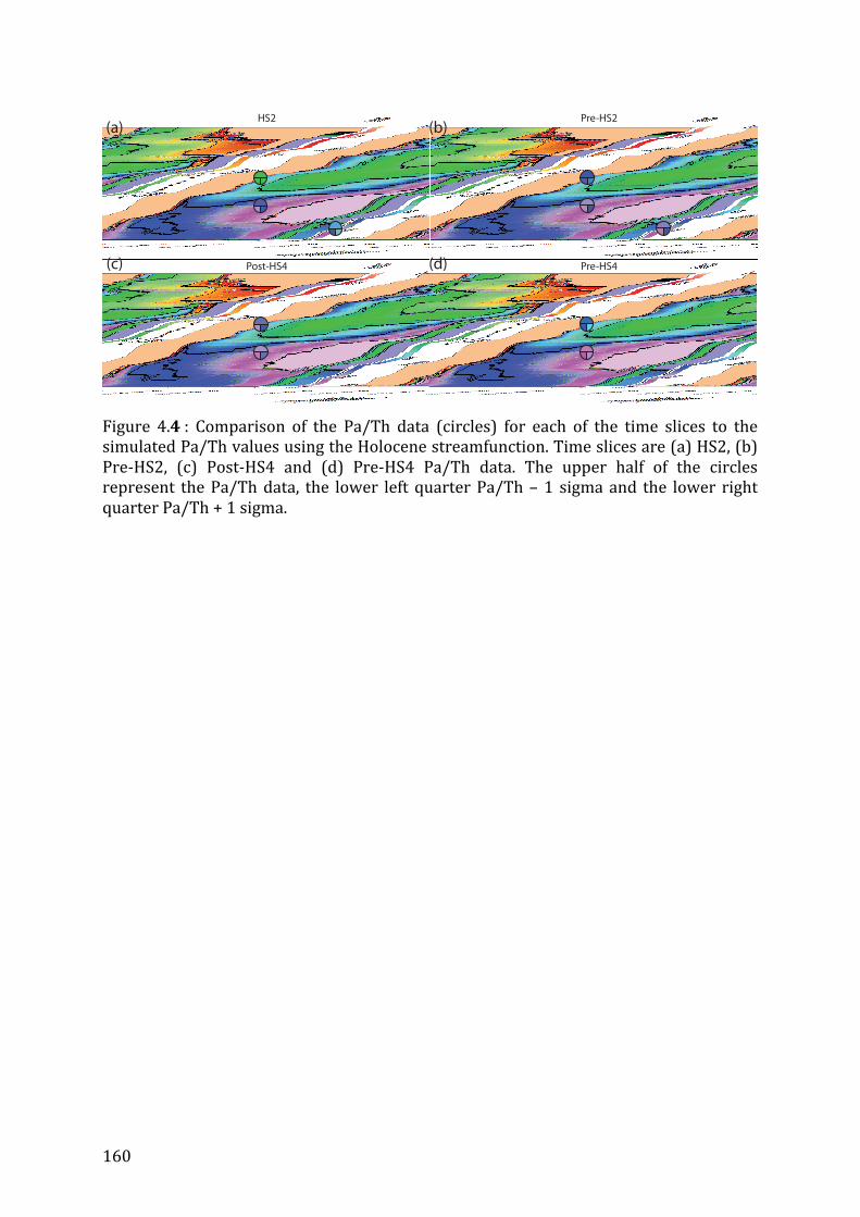
160

Figure 4.4 : Comparison of the Pa/Th data (circles) for each of the time slices to the simulated Pa/Th values using the Holocene streamfunction. Time slices are (a) HS2, (b)

Pre‐HS2, (c) Post‐HS4 and (d) Pre‐HS4 Pa/Th data. The upper half of the circles

represent the Pa/Th data, the lower left quarter Pa/Th – 1 sigma and the lower right

quarter Pa/Th + 1 sigma.

(a) (b)

(c) (d)

HS2 Pre-HS2

Post-HS4 Pre-HS4

161

Figure 4.5 : Comparison of the Pa/Th data for each of the time slices to the simulated

Pa/Th values using the off‐mode streamfunction. Time slices are (a) HS2, (b) Pre‐HS2,

(c) Post‐HS4 and (d) Pre‐HS4 Pa/Th data. The upper half of the circles represent the

Pa/Th data, the lower left quarter Pa/Th – 1 sigma and the lower right quarter Pa/Th +

1 sigma.

(a) (b)

(c) (d)

HS2 Pre-HS2

Post-HS4 Pre-HS4

162

Figure 4.6 : Comparison of the Pa/Th data for each of the time slices to the simulated Pa/Th values using the HS1 streamfunction. Time slices are (a) HS2, (b) Pre‐HS2, (c)

Post‐HS4 and (d) Pre‐HS4 Pa/Th data. The upper half of the circles represent the Pa/Th

data, the lower left quarter Pa/Th – 1 sigma and the lower right quarter Pa/Th + 1

sigma.

(a) (b)

(c) (d)

HS2 Pre-HS2

Post-HS4 Pre-HS4

163

Figure 4.7 : Sketch of the possible states of the AMOC during (a) DO interstadials and (b)

Heinrich Stadials. See text for explanation.

MD09-3257 (2300m)

MD09-3256Q (3500m)

?

Southern sourced water,

low δ13C

MD09-3257 (2300m)

MD09-3256Q (3500m)

?

Southern sourced water,

low δ13C

Northern sourced water,

high δ13C

(a)

(b)

Interstadials

Stadials

ODP Site1063 (4500m)

ODP Site 1063 (4500m)

2-10 Sv

2-10 Sv

164

4.3 Supporting Information

The supporting information provides additional figures, which further illustrate the

main text.

Supporting Information

Changes in the geometry and strength of the AMOC during the last glacial

P. Burckel, C. Waelbroeck, Y. Luo , D. Roche, S. Pichat, J. Gherardi, A. Govin, F. Thil

Figures

Figure 4.S1 : Pa/Th in MD09‐3256Q as a function of time calculated with different

lithogenic (238U/232Th) (R) values used to correct for detrital material contribution

(Francois, 2007). Red curve, R=0.5 (correction used in Fig. 3), green curve R=0.4, and

blue curve R=0.6. Error bars are 1 SD and do not account for the error on R.

165

Figure 4.S2 : Core MD09‐3256Q age model. Blue squares indicate the position of the 14C

dates in the core, blue triangles indicate tie points between core GeoB3910 and MD09‐

3256Q. Discontinuities in the Ti/Ca record correspond to the position of turbidite layers.

Error bars are 1 sigma and do not include the uncertainty on correlation for the tie

points.

0.00#

0.02#

0.04#

0.06#

0.08#

0.10#

0.12#

0.14#

0.0#

0.2#

0.4#

0.6#

0.8#

1.0#

1.2#

0# 5# 10# 15# 20# 25# 30# 35# 40# 45# 50#

Age#(ka)#

Ti/Ca#(GeoB3910)#

Ti/Ca#(MD09<3256Q)#

GeoB3910# MD09<3256Q#

166

Figure 4.S3 : Core MD09‐3256Q Ti/Ca (blue curve) and sedimentation rate (red curve).

0"

1"

2"

3"

4"

5"

6"

7"

8"

0"

0.02"

0.04"

0.06"

0.08"

0.1"

0.12"

0.14"

0" 5" 10" 15" 20" 25" 30" 35" 40" 45" 50"

Ti/Ca"

Sedim

enta7on"rate"(cm

.ky>1)"

Age"(ka)"

167

Figure 4.S4 : Sedimentary Pa/Th (red) and opal flux (black) as a function of depth in

core MD09‐3256Q. Error bars are 1 SE.

168

Figure 4.S5 : Correlation between the 232Th flux and sedimentary Pa/Th ratio on core MD09‐3256Q. White diamonds represent Pa/Th data that may not represent a pure

circulation signal.

169

Figure 4.S6 : Pa/Th of core MD09‐3257 (red), MD09‐3256Q (blue), ODP site 172

(Lippold et al., 2009)(green) and MD02‐2594 (Negre et al., 2010)(black). White symbols

represent Pa/Th data that may not reflect a pure circulation signal.

170

Figure 4.S7 : H1 simulated (a) Pa/Th and (b) streamfunction and flux (Sv, blue bars,

scale on top) at the equator. Note the large flow rate decrease at the equator from

~2500 m to ~3500 m.

00

0

00

0

-5-5

-5

-5

-5

-5

5

5

5

55

5

-10

-10

-10

-10

-10

-10-5

-5

-5

-5

-5

5

5

-15

-15

-15

-15

-20

-20

5

10

0

10

-25

Latitude

Dep

th


60S 50S 40S 30S 20S 10S 0 10N 20N 30N 40N 50N 60N

4750

4250

3750

3250

2750

2250

1750

1250

750

250

-25

-20

-15

-10

-5

0

5

10

(a)

H1 simulated Pa/Th

0

1000

2000

3000

4000

5000

10

5

0

-5

-10

-15

-20

-2560N30N030S60S

Ov

ertu

rnin

g ra

te (S

v)

(b)

H1streamfunction

-1.5 -1 -0.5 0 0.5 1 1.5 2 2.5 3

Flux(Sv)

171

Figure 4.S8 : Pa/Th on the Brazilian margin. Red squares, data obtained from Holocene

sediments in this study. Black squares, data obtained from Holocene sediments in

(Lippold et al., 2011). Grey and black lines, simulated Pa/Th values with the 2 and 3x

increased Holocene streamfunction respectively.

172

Tables

Table 4.S1 : Core MD09‐3256Q age model. 14C age is converted to calendar age using the Marine13 curve (Reimer et al., 2013) with no additional reservoir age correction. *

GeoB3910 tie points.

Depth (m) Age 14C (kyr) 1σ Age (Cal kyr) 1σ

0.040 2.32 0.03 1.93 0.04

0.580 15.97 0.06 18.82 0.06

0.660 17.72 0.06 20.88 0.11

0.880 20.5 0.08 24.16 0.12

0.920 21.41 0.08 25.36 0.12

0.960 22.87 0.08 26.79 0.18

* 1.115 / 30.61 0.16

* 1.585 / 39.03 0.50

* 1.945 / 47.91 0.51

Table 4.S2 : Pa/Th for each of the time slices at the different cores. Error bars are the maximum between standard deviation on Pa/Th values within the time slice and the

propagation of individual measurement errors on the averaged Pa/Th value defining the

time slice.

Table 4.S3 : Square root of the sum of squared difference between Pa/Th data and simulated value using the HS1 streamfunction intensified by various factors for the two

equatorial cores. The minimum values indicate the best agreement of the simulated

Pa/Th with the measured Pa/Th.

Factor Pre‐H2 Post‐H4 Pre‐H4

x0.5 2.9E‐02 3.5E‐02 3.5E‐02

x1 8.0E‐03 8.1E‐03 1.6E‐02

x1.5 1.8E‐02 1.0E‐02 2.0E‐02

x2 2.6E‐02 1.9E‐02 2.7E‐02

x3 3.5E‐02 2.8E‐02 3.4E‐02

Core Depth)(m) HS2)Pa/Th 1σ Pre6HS2)Pa/Th 1σ Post6HS4)Pa/Th 1σ Pre6HS4)Pa/Th 1σ

MD0963257 2344 0.103 0.003 0.071 0.004 0.066 0.004 0.075 0.005

MD0963256Q 3537 0.068 0.005 0.064 0.005 0.063 0.003 0.059 0.003

ODP)site)1063 4584 0.079 0.010 0.065 0.004 / /

173

Table 4.S4 : Pa/Th and isotopic concentrations (dpm.g‐1) in core MD09‐3256Q

Depth (m) Age( Cal kyr BP) 1 σ 231Pa 1 σ 230Th 1 σ 232Th 1 σ 238U 1 σ Pa/Th 1 σ

0 0.50 0.50 0.240 0.003 5.51 0.11 1.19 0.02 1.085 0.007 0.043 0.001

0 0.50 0.50 0.240 0.004 5.52 0.08 1.20 0.02 1.082 0.006 0.043 0.001

0.88 24.16 0.12 0.181 0.003 3.76 0.07 3.46 0.05 1.906 0.011 0.066 0.003

0.89 24.46 0.12 0.241 0.004 4.92 0.08 3.40 0.05 1.804 0.018 0.067 0.002

0.9 24.76 0.12 0.247 0.004 5.09 0.11 2.76 0.04 1.346 0.007 0.066 0.002

0.9 24.76 0.12 0.245 0.004 5.14 0.11 2.64 0.04 1.333 0.007 0.065 0.002

0.92 25.37 0.12 0.259 0.004 5.36 0.12 2.57 0.04 1.255 0.010 0.067 0.002

0.94 26.08 0.15 0.267 0.004 5.45 0.12 2.63 0.05 1.381 0.008 0.068 0.002

0.96 26.79 0.18 0.254 0.004 5.38 0.11 2.56 0.05 1.432 0.007 0.065 0.002

0.98 27.28 0.17 0.242 0.004 5.20 0.09 2.45 0.03 1.314 0.012 0.064 0.002

1.46 36.79 0.41 0.151 0.003 3.41 0.06 1.90 0.03 1.129 0.024 0.066 0.003

1.48 37.15 0.43 0.153 0.003 3.55 0.08 1.94 0.04 1.121 0.015 0.064 0.003

1.5 37.50 0.44 0.151 0.004 3.59 0.07 2.14 0.03 1.392 0.010 0.061 0.003

1.5 37.50 0.44 0.152 0.004 3.53 0.06 2.00 0.03 1.365 0.019 0.063 0.003

1.51 37.68 0.45 0.160 0.003 3.64 0.07 2.02 0.03 1.600 0.031 0.064 0.003

1.56 38.58 0.49 0.226 0.004 4.55 0.07 2.59 0.04 2.115 0.018 0.078 0.003

1.57 38.76 0.49 0.233 0.004 4.81 0.07 2.91 0.03 1.822 0.013 0.077 0.003

1.58 38.94 0.50 0.232 0.003 4.82 0.09 3.04 0.05 1.748 0.014 0.077 0.003

1.59 39.15 0.50 0.235 0.004 4.66 0.11 2.94 0.06 1.643 0.015 0.083 0.004

1.59 39.15 0.50 0.213 0.005 4.67 0.08 2.88 0.04 1.635 0.012 0.072 0.003

1.6 39.40 0.50 0.230 0.004 4.71 0.09 3.05 0.03 1.493 0.012 0.080 0.003

1.61 39.64 0.50 0.186 0.003 4.27 0.09 2.45 0.04 1.267 0.008 0.068 0.003

1.62 39.89 0.50 0.176 0.003 4.14 0.07 2.33 0.03 1.291 0.011 0.065 0.003

1.63 40.14 0.50 0.156 0.003 3.80 0.06 2.04 0.03 1.270 0.009 0.061 0.002

1.64 40.38 0.50 0.150 0.004 3.74 0.06 2.00 0.02 1.245 0.022 0.060 0.003

1.66 40.88 0.51 0.146 0.004 3.76 0.09 2.04 0.04 1.350 0.008 0.056 0.003

1.68 41.37 0.51 0.148 0.004 3.66 0.07 2.05 0.03 1.209 0.009 0.061 0.003

174

Table 4.S5 : Core MD09‐3256Q δ13C (C. wuellerstorfi)

Additional references





doi:10.1029/2011GL049282, 2011.






Maximum, Nature, 468, 84‐+, 2010.







Age (Cal kyr BP) Depth (m) ∂13C (‰) Age (Cal kyr BP) Depth (m) ∂13C (‰) Age (Cal kyr BP) Depth (m) ∂13C (‰)

1.93 0.04 1.29 35.00 1.36 0.32 38.58 1.56 0.39

1.93 0.04 1.33 35.00 1.36 0.89 38.58 1.56 0.97

1.93 0.04 1.32 35.71 1.4 0.65 38.76 1.57 0.40

1.93 0.04 1.38 35.71 1.4 0.53 38.76 1.57 0.02

1.93 0.04 1.38 35.89 1.41 0.77 38.94 1.58 0.38

24.16 0.88 0.30 35.89 1.41 -0.11 38.94 1.58 0.19

24.46 0.89 -0.16 36.07 1.42 0.56 38.94 1.58 0.93

25.06 0.91 0.34 36.07 1.42 -0.35 39.15 1.59 0.34

25.37 0.92 0.10 36.07 1.42 0.40 39.40 1.6 0.55

25.72 0.93 0.12 36.25 1.43 -0.16 39.64 1.61 0.31

26.08 0.94 0.39 36.25 1.43 0.40 39.89 1.62 0.21

26.43 0.95 0.31 36.25 1.43 0.66 39.89 1.62 0.29

26.79 0.96 0.23 36.43 1.44 0.61 40.14 1.63 0.30

27.03 0.97 0.39 36.43 1.44 0.62 40.38 1.64 0.38

27.28 0.98 0.44 36.61 1.45 0.85 40.63 1.65 0.27

27.53 0.99 0.20 36.61 1.45 0.92 40.63 1.65 0.52

27.77 1 0.07 36.79 1.46 0.66 40.88 1.66 0.13

28.27 1.02 0.25 36.79 1.46 0.86 41.12 1.67 0.33

28.76 1.04 0.15 36.97 1.47 0.24 41.12 1.67 0.57

29.25 1.06 0.40 36.97 1.47 0.03 41.37 1.68 0.71

29.75 1.08 0.34 37.15 1.48 0.39 41.37 1.68 0.80

30.24 1.1 0.48 37.15 1.48 0.83 41.62 1.69 0.55

30.70 1.12 0.45 37.33 1.49 0.80 41.62 1.69 0.41

31.06 1.14 0.35 37.33 1.49 0.48 41.86 1.7 0.77

31.42 1.16 0.68 37.50 1.5 0.86 41.86 1.7 0.88

31.78 1.18 0.25 37.50 1.5 0.70 42.36 1.72 1.20

32.13 1.2 0.62 37.68 1.51 1.01 42.36 1.72 0.28

32.49 1.22 0.33 37.68 1.51 0.33 42.85 1.74 0.98

32.85 1.24 0.68 37.86 1.52 0.67 43.35 1.76 0.80

33.21 1.26 0.70 38.04 1.53 0.26 43.84 1.78 0.73

33.21 1.26 0.50 38.04 1.53 0.51 43.84 1.78 0.56

33.57 1.28 0.41 38.22 1.54 0.87 44.33 1.8 0.33

33.92 1.3 0.48 38.22 1.54 0.09 44.33 1.8 0.70

34.28 1.32 0.17 38.40 1.55 0.23

34.64 1.34 0.77 38.40 1.55 0.41

175

Chapter 5: Conclusion and perspectives

5.1 Conclusion

The first objective of this thesis was to reconstruct the dynamics of the Atlantic

Meridional Overturning Circulation during the last glacial. In order to do that, I

measured the sedimentary Pa/Th ratio, a proxy of water mass renewal rate, in two

sediment cores of the equatorial Atlantic. I also measured the benthic δ13C, which

provides information about the nutrient content of water masses, in one of the two

cores. The Pa/Th and benthic δ13C are complementary and provide information about

the flow rate and ventilation of water masses respectively.

The second objective of this thesis was to investigate the relationship between AMOC

variations and climate. In order to do that, I first built an age model for both equatorial

sediment cores that is entirely radiometric and independent of the GICC05 age scale. I

then compared the flow rate and ventilation of the water masses influencing my

sediment cores during the last glacial to Greenland temperature and tropical

precipitation.

My results show that the vertical layout and strength of the water masses constituting

the AMOC changed over the course of the last glacial. In this conclusion, I summarize

each of the results presented in this thesis and classify them based on their associated

climatic period.

5.1.1 DansgaardOeschger interstadials

During Dansgaard‐Oeschger interstadials, two circulation cells were likely active in the

Atlantic Ocean (Chapter 4.2). A first circulation cell was initiated by deep convection in

the northern North Atlantic, and consisted of a deep‐water mass circulating southwards

above ~2500 m depth. This northern‐sourced water mass was likely characterized by

flow rates of 2‐10 Sv at the equator, which is lower than the flow rate of present day

NADW (i.e. 23 ± 3 Sv (Ganachaud and Wunsch, 2000)). A second circulation cell was

initiated in the Southern Ocean by the formation of a deep‐water mass, which flowed

northwards below 4000 m depth, and reached at least 35°N at 4500 m depth. The flow

rate of this southern sourced water mass was likely of 2‐10 Sv, which encompasses the

strength of modern AABW (i.e. 6 ± 1.3 Sv, (Ganachaud and Wunsch, 2000)). Between

2500 and 4000 m depth at the equator, the southern‐sourced water mass circulated

southwards as a return flow.

176

5.1.2 Heinrich Stadials

As detailed in Chapter 3, a southward shift of the Inter Tropical Convergence Zone is

simulated in climate models either through a slowdown of the AMOC upper circulation

cell, or through the development of sea ice and ice sheets in the high latitudes of the

northern Hemisphere. My results show that the Pa/Th signal at 2300 m on the Brazilian

margin rises 1420 ± 250 (1σ) and 690 ± 180 (1σ) y before the onset of the precipitation

events associated with HS2 and HS4 respectively (Chapter 3). I interpret the Pa/Th rise

as a decrease in the flow rate of the upper overturning cell of the AMOC. Hence, I confirm

that a reduction of the oceanic inter‐hemispheric heat transport could be at the origin of

the ITCZ shifts occurring during Heinrich Stadials.

These large leads contrast with model results, which show that 50% of the final tropical

precipitation anomaly occurs only 200 y after the start of an AMOC slowdown in

response to freshwater input in the high latitude North Atlantic (Kageyama et al., 2009).

Such a rapid response of the tropical atmosphere in the model could be related to the

fast simulated AMOC slowdown, as minimum overturning rate is achieved only 400 y

after the start of the slowdown. A more gradual decrease of the flow rate could lead to a

delayed establishment of the SST anomaly required for the ITCZ to shift above the

Brazilian margin, in agreement with our data.

We now consider the structure of the AMOC during the Heinrich Stadials following the

gradual slowdown of the AMOC upper circulation cell that likely caused the southward

ITCZ shifts. My data at the onset of HS2 show that the layout of the equatorial water

masses at that time was significantly different from that of preceding DO interstadials

(Chapter 4). Below 1300 m depth, the Atlantic Ocean was likely dominated by a

southern sourced water mass that reached at least 35°N at 4500 m depth. The southern

sourced water mass probably directly affected the equator between 2500‐3500 m

depth. Sluggish and poorly ventilated waters of unknown origin likely influenced the

equatorial Atlantic between 1300 and 2300 m depth.

My results do not show major differences between HS2 and HS4, despite the large

difference in Northern hemisphere ice sheet extent between these two periods. In both

cases, the slowdown of the upper AMOC circulation cell precedes the southward ITCZ

shift (Chapter 3). However, I was not able to assess the strength and geometry of the

AMOC during HS4 because, at that time, Pa/Th data in both equatorial cores could not

reflect a pure circulation signal (Chapter 4). Hence, I cannot conclude that both Heinrich

Events are similar in terms of AMOC configuration. The only difference between the two

periods is that the benthic δ13C of the preceding and following interstadials is higher for

HS4 than for HS2 (Chapter 4), which might be related to the more developed continental

biosphere occurring during early MIS3 (Duplessy et al., 1988).

177

5.1.3 Dansgaard Oeschger Stadials

During Dansgaard‐Oeschger stadials, the flow rate of the AMOC upper circulation cell

likely decreased, but less than during HS2. At the same time, increased precipitation is

observed on the Brazilian margin, although the associated terrigenous input was smaller

than during Heinrich Stadials. These periods of increased precipitation also correspond

to clear decreases in South American speleothem δ18O attributed to southward ITCZ

shifts (Kanner et al., 2012). However, there is no significant lead of the oceanic

circulation signal with respect to the ITCZ shifts. Both the AMOC and Greenland

temperature changes appear to be in phase with increased precipitation. A short time

lag of increased tropical precipitation with respect to decreased Greenland temperature

would be consistent with atmospheric processes driving the ITCZ shifts associated with

DO‐stadials. However, slowdowns of the AMOC upper circulation cell also occur during

DO‐stadials. Based on these evidences, it is difficult to infer what processes were at the

origin of the small ITCZ shifts associated to DO‐stadials.

5.1.4 Mechanisms of climate variability

5.1.4 a) Difference between Dansgaard Oeschger and Heinrich Stadials

Based on the large lead of the upper AMOC circulation cell slowdown with respect to the

ITCZ shifts associated with Heinrich Stadials, we proposed a mechanism to explain the

difference between Heinrich and DO stadials. During Heinrich Stadials, an initial

decrease in the overturning rate of the upper overturning cell of the AMOC could have

led to a warming of subsurface waters in the North Atlantic Ocean (Mignot et al., 2007).

This could have resulted in the destabilization of high latitude North Atlantic ice shelves,

leading to the calving of the Laurentide ice sheet (Alvarez‐Solas et al., 2013). This input

of freshwater would have further reduced the intensity of the upper circulation cell of

the AMOC, leading to further subsurface warming and ice calving. This positive feedback

would have progressively reduced the flow rate of the AMOC upper circulation cell and

heat transport towards the high latitude North Atlantic, thereby pushing the ITCZ to an

increasingly southerly position. In contrast, the circulation slowdown occurring during

DO stadials would have been unable to trigger the aforementioned feedback. Thus, both

the decreased intensity of the upper circulation cell of the AMOC and the southward

shift of the ITCZ remained limited. Hence, during Heinrich Stadials, the large iceberg

discharges associated with the positive feedback described above could have resulted in

the deposition of large quantities of IRD in the high latitude North Atlantic. This

mechanism could explain the thick and thin IRD layers observed during Heinrich and DO

Stadials respectively.

178

5.1.4 b) Effect of the AMOC on Greenland temperatures

My results also show that, although the AMOC is an important source of heat for the high

latitude North Atlantic, the temperature response of Greenland to a slowdown of the

AMOC upper circulation cell is largely modulated by other processes.

Indeed, no major Greenland air temperature variations occur during the decreased

AMOC flow rate associated with HS2. It suggests the importance of other processes in

regulating Greenland temperatures. Sea ice for instance, during periods of cold

Greenland temperatures preceding HS2, could have acted on Greenland as an insulator,

preventing further temperature decrease with decreasing heat transport (Li et al.,

2010).

Moreover, heat transport by atmospheric processes could be increased during periods

of decreased oceanic heat transport (Kageyama et al., 2009; Shaffrey and Sutton, 2006).

Indeed, decreased oceanic heat transport could result in decreased SST in the high

latitude North Atlantic, hence increasing the meridional temperature gradient. This

would increase baroclinicity of the atmosphere, leading to higher atmospheric heat

transport to the high latitude North Atlantic (van der Swaluw et al., 2007). Increased

atmospheric heat transport could therefore partly compensate for the decreased oceanic

heat transport.

5.2 Perspectives

The results of this thesis provide new insights into the deep Atlantic circulation during

the last glacial. Unfortunately, we could not analyze the Pa/Th signal of shallow

sedimentary cores (Chapter 1). Pa/Th measurements in shallow sediment cores (~1000

m depth) would be extremely valuable to improve our understanding of the changes in

the AMOC upper overturning cell flow rate during the last glacial. More specifically, it

could serve to verify if a decreased southward flow rate at 2300 m depth is also

accompanied by a decreased northward flow rate and heat export in surface waters.

Analyses of the Pa/Th ratio of new sediment cores along latitudinal sections or depth

transects in the Atlantic Ocean during the last glacial would help better constraining the

geometry and flow rate of the water masses constituting the AMOC. It would probably

allow a more accurate quantification of overturning rates during Dansgaard‐Oeschger

interstadials, and provide information on the southern‐sourced water mass flow rate

during Heinrich Stadials.

In order to better understand the evolution of the ITCZ during Heinrich and DO stadials,

a careful estimation of the lead of decreased precipitation in the northern tropics with

179

respect to increased precipitation in the southern tropics would be required. Indeed, the

mechanisms of ITCZ variability could likely be discriminated based on the rapidity of the

ITCZ shifts The slowly decreasing oceanic meridional heat transport that we propose

would for instance be reflected by a gradual southward ITCZ shift, unless SST anomalies

need to reach a certain threshold for the tropical convection zone to shift. Such a study

would require a precise chronological framework, and would likely be possible using

varved sediments or speleothems, which can be dated with a precision of a few decades

even during the last glacial.

Finally, correlation of high latitude North Atlantic SST signals to Greenland

temperatures would allow placing the periods of IRD deposition on the GICC05

timescale. Because the age model of our sediment cores is completely independent from

the GICC05 timescale, we could directly compare the timing of iceberg releases related

to Heinrich and precursory events (Peck et al., 2006) to periods of decreased strength of

the upper AMOC circulation cell. Hence, it could be possible to determine whether the

circulation slowdown observed in the Atlantic Ocean are the cause or the consequence

of iceberg releases.

181

LIST OF FIGURES AND TABLES

Figures

FIGURE 1 : GREENLAND AIR TEMPERATURES OF THE LAST 20‐50 KA (KINDLER ET AL., 2014).

NUMBERS INDICATE DANSGAARD‐OESCHGER INTERSTADIALS AND HS INDICATES HEINRICH

STADIALS. 15 FIGURE 2 : SKETCH OF THE ATLANTIC MERIDIONAL OVERTURNING CIRCULATION (AMOC) FROM

(KUHLBRODT ET AL., 2007). BLUE ARROWS INDICATE THE APPROXIMATE FLOW DIRECTION OF

NADW (NORTH ATLANTIC DEEP WATER) AND AABW (ANTARCTIC BOTTOM WATER), THE

NORTHERN AND SOUTHERN SOURCED DEEP WATER MASSES INITIATING THE UPPER AND

LOWER OVERTURNING CELLS OF THE AMOC RESPECTIVELY. 16 FIGURE 1.1 : DISSOLVED 231PA AND 230TH PROFILES IN THE EQUATORIAL ATLANTIC FROM (CHOI ET

AL., 2001). NOTE THAT THE 230TH PROFILE INCREASES LINEARLY WITH DEPTH AS PREDICTED BY

REVERSIBLE SCAVENGING, WHILE PROTACTINIUM IS EXPORTED AT DEPTH, RESULTING IN AN

ALMOST CONSTANT CONCENTRATION WITH DEPTH BELOW 1000 M. 26 FIGURE 1.2 : STUDY AREA AND POSITION OF THE MAIN SURFACE CURRENTS (MODIFIED FROM

(FRATANTONI AND GLICKSON, 2002)) 29 FIGURE 1.3 : SURFACE CURRENTS DURING APRIL (TOP) AND NOVEMBER (BOTTOM). DURING TIMES OF

MINIMUM NECC INTENSITY (APRIL), AMAZON WATERS ARE DEVIATED NORTHWARDS. DURING

TIMES OF MAXIMUM NECC (NOVEMBER), AMAZON WATERS ARE DEVIATED EASTWARDS BUT DO

NOT REACH OUR STUDY AREA (LUMPKIN AND GARZOLI, 2005). 30 FIGURE 1.4 : MAP OF THE NORTH EASTERN BRAZILIAN MARGIN. NAMES OF RETRO3 CORES ARE

WRITTEN IN RED AND NAMES OF M34/4 CORES IN GREEN. 32 FIGURE 1.5 : PHOSPHATE SECTION OF THE ATLANTIC OCEAN SHOWING THE SITES OF THE CORES

LISTED IN TABLE 1. WHITE ARROWS INDICATE THE APPROXIMATE FLOW DIRECTIONS OF THE

ANTARCTIC INTERMEDIATE WATER (AAIW), ANTARCTIC BOTTOM WATER (AABW) AND NORTH

ATLANTIC DEEP WATER (NADW). 33 FIGURE 1.6 : TI/CA RECORD OF CORE GEOB3910. EACH TI/CA PEAK IS ASSOCIATED WITH ONE

HEINRICH STADIAL (HS1‐5). 34 FIGURE 1.7 : (A) Δ18O AND (B) TI/CA SIGNALS OF INTERMEDIATE DEPTH CORES ON THE GEOB3910

DEPTH SCALE. 35 FIGURE 1.8 : (A) TI/CA AND (B) 14C DATES (MARINE13, (REIMER ET AL., 2013)) IN CORE MD09‐3257 35 FIGURE 1.9 : (A) Δ18O AND (B) TI/CA SIGNALS OF INTERMEDIATE (GEOB3910) AND DEEP (MD09‐

3256Q) CORES ON THE GEOB3910 DEPTH SCALE. NOTE THAT CORRELATION OF HS2 BETWEEN

CORE MD09‐3256Q AND CORE GEOB3910 REVEALED TO BE INCORRECT, AS INFERRED FROM 14C

DATING. 37 FIGURE 1.10 : PRESENT DAY TEMPERATURE AND SALINITY AT 30 M DEPTH ON THE BRAZILIAN

MARGIN (WOA09). 37 FIGURE 1.11 : (A) TI/CA AND (B) 14C DATES (MARINE13, (REIMER ET AL., 2013)) IN CORE MD09‐3256Q

38 FIGURE 1.12 : (A) Δ18O AND (B) TI/CA SIGNALS IN SHALLOW SEDIMENT CORES. 39 FIGURE 2.1 : SI (MG) AS A FUNCTION OF ABSORBANCE. SI CONTENT OF A SAMPLE SOLUTION IS

ESTIMATED BASED ON ITS MEASURED ABSORBANCE AND ON THE RELATION ABSORBANCE‐

WEIGHT(SI) OF THE STANDARDS. 44 FIGURE 2.2 : EXTRACTION OF SI AS A FUNCTION OF TIME IN A SEDIMENT SAMPLE CONTAINING

BIOGENIC SILICA AND ALUMINO‐SILICATE. AFTER 1‐2H, ALL BIOGENIC SILICA IS DISSOLVED

(DEMASTER, 2013). SI LEACHING CONTINUES AT A CONSTANT RATE, WHICH ALLOWS FINDING

THE INITIAL %SI BIOGENIC IN THE SAMPLE FROM THE INTERCEPT. 44 FIGURE 2.3 : %OPAL IN TWO SAMPLES MEASURED BOTH AT THE IUP (BLUE DIAMONDS) AND LSCE

(RED SQUARES). 45 FIGURE 2.4.1 : ANION‐EXCHANGE CHROMATOGRAPHY SEPARATION AND PURIFICATION USED BY EACH

OF THE PARTICIPATING LABORATORIES. HCL CONCENTRATION IS 9N, HNO3 8N AND HF 0.13N

UNLESS OTHERWISE STATED. RESIN TYPES INDICATED FOR THE LAST CHROMATOGRAPHY

COLUMN OF EACH LABORATORY ALSO STAND FOR THE PREVIOUS COLUMNS OF THE

LABORATORY. 68

182

FIGURE 2.4.2 : ISOTOPIC RATIOS MEASURED BY EACH LABORATORY ON THORIUM AND URANIUM

ISOTOPIC REFERENCE MATERIAL. (A) 230TH/232TH MEASURED ON IRMM‐035. CERTIFIED VALUE IS

GIVEN AS REFERENCE, AS WELL AS INTER‐LABORATORY MC‐ICP‐MS VALUE FROM SIMS ET AL 29.

(B) 234U/238U MEASURED ON NBS‐SRM‐960. CERTIFIED VALUE IS GIVEN AS REFERENCE. THE IUP

GROUP MEASURED NBS‐SRM‐960 TWICE, ON SOLUTIONS FROM TWO DIFFERENT BOTTLES.

ERROR BARS ARE THE MAXIMUM BETWEEN 2SE PROPAGATED ON THE MEAN (ERROR ON THE

SUM OF REPLICATE MEASUREMENTS DIVIDED BY THE NUMBER OF MEASUREMENTS) AND 2SD

ON SAMPLE REPLICATES (STANDARD DEVIATION OF REPLICATE MEASUREMENTS). THE NUMBER

OF FULL CHEMISTRY REPLICATES USED TO CALCULATE THE MEANS IS WRITTEN NEXT TO EACH

MEASUREMENT. 69 FIGURE 2.4.3 : COMPARISON OF THE 231PA CONCENTRATIONS IN SEDIMENT AND UREM11. RESULTS

ARE EXPRESSED BY THE DEVIATION (%)OF THE CONCENTRATIONS MEASURED BY EACH

LABORATORY FROM THE MEAN OF THE 4 LABORATORIES. THE DEVIATION OF THE GEOTRACES

INTERCALIBRATION VALUE FROM THE MEAN IS ALSO GIVEN FOR GEOTRACES_SED 23. NOTE THAT

THE GEOTRACES INTERCALIBRATION VALUE WAS NOT USED TO COMPUTE THE MEAN ISOTOPIC

CONCENTRATIONS. ERROR BARS ARE CALCULATED AS IN FIGURE 2 AND CONVERTED IN % FROM

THE INTER‐LABORATORY MEAN. THE NUMBER OF REPLICATES USED TO CALCULATE THE

AVERAGES IS WRITTEN NEXT TO THE ERROR BARS. 70 FIGURE 2.4.4 : COMPARISON OF THE (A) THORIUM AND (B) URANIUM CONCENTRATIONS IN SEDIMENT

AND UREM11. RESULTS ARE EXPRESSED BY THE DEVIATION (%) OF THE CONCENTRATIONS

MEASURED BY EACH LABORATORY FROM THE MEAN OF THE 4 LABORATORIES. IN (A), THE

DEVIATION OF THE GEOTRACES INTERCALIBRATION VALUE FROM THE MEAN IS ALSO GIVEN FOR

GEOTRACES_SED 23. NOTE THAT THE GEOTRACES INTERCALIBRATION VALUE WAS NOT USED TO

COMPUTE THE MEAN THORIUM ISOTOPIC CONCENTRATIONS. ERROR BARS ARE CALCULATED AS

IN FIGURE 2 AND CONVERTED IN % FROM THE INTER‐LABORATORY MEAN. MEAN

CONCENTRATIONS FOR EACH LAB WERE CALCULATED USING THREE FULL REPLICATES UNLESS

WRITTEN OTHERWISE ON THE FIGURE. 71 FIGURE 2.4.5 : ISOTOPIC CONCENTRATIONS OBTAINED AT UB AFTER DIGESTION BY MICROWAVE

(WHITE CIRCLES) OR HOTPLATE (BLACK CIRCLES) ON (A) UREM11, (B) GEOTRACES_SED. ERROR

BARS ARE CALCULATED AS IN FIGURE 2 FOR MICROWAVE MEASUREMENTS. ERROR BARS ARE

2SE FOR HOTPLATE MEASUREMENTS (1 REPLICATE ONLY). ERROR BARS ON HOTPLATE

MEASUREMENTS ON THE GEOTRACES_SED SAMPLE ARE SMALL AND CANNOT BE DISTINGUISHED

FROM THE DATA POINTS. 72 FIGURE 2.4.6 : CONCENTRATION DEVIATIONS OF ONE REPLICATE FROM THE OTHER AS A FUNCTION

OF ADDITIONAL TIME LEFT FOR 233PA TO DECAY IN THE SECOND REPLICATE (SEE TEXT).

REPLICATES REPRESENTED BY THE SQUARE ARE NOT FULL CHEMISTRY REPLICATES, BUT A

SINGLE PA FRACTION THAT WAS MEASURED AT DIFFERENT TIMES AFTER U‐PA SEPARATION (10

AND 52 DAYS). REPLICATES REPRESENTED BY THE CIRCLES ARE FULL CHEMISTRY REPLICATES.

NUMBERS INDICATE THE AVERAGE CONCENTRATIONS OF THE REPLICATES (DPM.G‐1). SEE TABLE

S3 FOR UNCERTAINTIES ON 231PA MEASUREMENTS. 73 FIGURE 2.4.S1 : ILLUSTRATION OF THE CONING AND QUARTERING METHOD. FIRST, A) THE SEDIMENT

IS POURED ON DRAWING PAPER BY APPLYING A SWIRLING MOVEMENT TO THE WRIST IN ORDER

TO FORM A DOME THEN B) THE DOME IS DIVIDED IN FOUR AND C) THE OPPOSITE QUARTERS

ARE GATHERED. THE RESULTING SEDIMENT PILES (2, 3) AND THE INITIAL SEDIMENT (1) ARE

EXPECTED TO BE HOMOGENEOUS. 79 FIGURE 2.4.S2 : SEDIMENT AND UREM11 232TH CONCENTRATION RESULTS FOR EACH OF THE

PARTICIPATING LABORATORIES. NOTE THAT THE Y AXIS RANGE FOR EACH SAMPLE IS OF

AROUND 25% OF THE SAMPLE’S MEAN CONCENTRATION. THIS ALLOWS TO COMPARE THE INTER

AND INTRA‐LABORATORY CONCENTRATION VARIABILITY OF THE SAMPLES. HENCE CARE

SHOULD BE TAKEN WHEN COMPARING ABSOLUTE CONCENTRATIONS, AS THE Y AXIS IS OFTEN

SPLIT AND MAGNIFIED FOR SOME SAMPLES. CIRCLES REPRESENT THE UREM11, SQUARES THE

GEOTRACES_SED AND DIAMONDS THE MARGIN_SED SAMPLES. ERROR BARS ARE 2SE. 80 FIGURE 2.4.S3 : SEDIMENT AND UREM11 230TH CONCENTRATION RESULTS FOR EACH OF THE






GEOTRACES_SED AND DIAMONDS THE MARGIN_SED SAMPLES. ERROR BARS ARE 2SE. 81

183

FIGURE 2.4.S4 : SEDIMENT AND UREM11 238U CONCENTRATION RESULTS FOR EACH OF THE






GEOTRACES_SED AND DIAMONDS THE MARGIN_SED SAMPLES. ERROR BARS ARE 2SE. 82 FIGURE 2.4.S5 : SEDIMENT AND UREM11 234U CONCENTRATION RESULTS FOR EACH OF THE






GEOTRACES_SED AND DIAMONDS THE MARGIN_SED SAMPLES. ERROR BARS ARE 2SE. 83 FIGURE 2.4.S6 : SEDIMENT AND UREM11 231PA CONCENTRATION RESULTS FOR EACH OF THE






GEOTRACES_SED AND DIAMONDS THE MARGIN_SED SAMPLES. ERROR BARS ARE 2SE. 84 FIGURE 2.4.S7 : MEAN PA/TH VALUES OBTAINED BY EACH OF THE PARTICIPATING LABS. NOTE THAT

THE Y AXIS RANGE FOR BOTH SAMPLES IS OF AROUND 25% OF THE SAMPLE’S MEAN PA/TH. THIS

ALLOWS TO COMPARE THE INTER‐LABORATORY PA/TH VARIABILITY OF THE SAMPLES. HENCE

CARE SHOULD BE TAKEN WHEN COMPARING ABSOLUTE PA/TH VALUES, AS THE Y AXIS IS SPLIT

AND MAGNIFIED. SQUARES REPRESENT THE GEOTRACES_SED AND DIAMONDS THE MARGIN_SED

SAMPLES. 2 SIGMA ERROR IS CALCULATED BASED ON THE MAXIMUM BETWEEN 2 SE AND 2 SD OF

REPLICATE CONCENTRATION MEASUREMENTS AND DOES NOT INCLUDE THE UNCERTAINTY ON

THE R VALUE (SET TO 0.5). 85 FIGURE 3.1 : MAP OF THE STUDY AREA. THE RED CIRCLE INDICATES THE LOCATION OF THE STUDIED

MARINE SEDIMENT CORES, THE ORANGE CIRCLE INDICATES THE POSITION OF THE EL CONDOR

(ELC) AND DIAMANTE (NAR) CAVES (10), THE BLACK DASHED LINE DELIMITATES THE

NORDESTE REGION, AND RED DASHED LINE SHOWS THE POSITION OF THE PRESENT DAY

SEPTEMBER AND MARCH ITCZ OVER THE ATLANTIC AND PACIFIC OCEAN. THE COLOR SCALE

INDICATES MEAN PRECIPITATION OVER SOUTH AMERICA (MM/Y) FOR THE MONTHS OF MARCH

AND SEPTEMBER AVERAGED OVER THE PERIOD 1950‐1996 AD (58). 111 FIGURE 3.2 : COMPARISON BETWEEN (A) THE U‐TH DATED δ18O RECORDS OF ELC/NAR SPELEOTHEMS

(10) AND (B) THE 14C‐DATED TI/CA RECORD OF CORE GEOB3910 (12). (C) TI/CA RECORD OF

MARINE SEDIMENT CORES GEOB3910 (12) AND MD09‐3257 ON THEIR FINAL AGE MODELS.

COLORED DIAMONDS SHOW THE POSITIONS OF THE U‐TH DATES FOR SPELEOTHEMS AND OF

THE 14C DATES FOR MARINE SEDIMENT CORES WITH THEIR 2 SD ERROR BARS. DIAMONDS

BELOW THE X‐AXIS DEPICT THE 14C DATES USED TO ESTABLISH THE AGE MODEL OF CORES

MD09‐3257 AND GEOB3910, DIAMOND COLORS CORRESPOND TO THAT OF THE CORES ON WHICH

THE 14C DATES HAVE BEEN MEASURED. EMPTY SQUARES SHOW THE POSITION OF GEOB3910‐

MD09‐3257 TIE POINTS USED TO ESTABLISH THE AGE MODEL OF CORE MD09‐3257. EMPTY

TRIANGLES ARE THE SPELEOTHEM TIE POINTS USED TO ESTABLISH THE AGE MODEL OF CORES

MD09‐3257 AND GEOB3910 BEYOND THE 14C DATING RANGE (SEE TEXT AND SI TABLE S1, S2).

112 FIGURE 3.3 : COMPARISON BETWEEN GREENLAND (A) NGRIP TEMPERATURE SIGNAL ON THE GICC05

TIMESCALE (59) AND BRAZIL (B) MD09‐3257 PA/TH, (C) GEOB3910 CIBICIDES WUELLERSTORFI

δ13C, AND (D) GEOB3910 (12) (BLUE) AND MD09‐3257 (RED) TI/CA RECORDS. GRAY DASHED

BANDS DELIMITATE THE PRECIPITATION EVENTS DEFINED ON THE ELC SPELEOTHEM δ18O

RECORD (SI APPENDIX FIG. S3). BLUE SHADED BANDS DELIMITATE THE PRECIPITATION EVENTS

AS SEEN IN THE MD09‐3257 TI/CA RECORD (SEE TEXT). VERTICAL BLACK DASHED LINES

INDICATE THE START OF THE PA/TH AND TI/CA RISES IN CORE MD09‐3257. IN (A) NUMBERS

INDICATE THE DO EVENTS. IN (B) THE RED LINE PASSES THROUGH AVERAGE PA/TH VALUES

WHEN THERE ARE REPLICATE MEASUREMENTS, THE WHITE SYMBOLS INDICATE PA/TH VALUES

ARE NOT CONSIDERED FOR THIS STUDY AS THEY MIGHT NOT REPRESENT A PURE CIRCULATION

SIGNAL (METHODS), THE RED HORIZONTAL BAND INDICATES THE PRESENT DAY PA/TH VALUE

184

(0.065±0.003, METHODS). ERROR BARS ON PA/TH MEASUREMENTS ARE GIVEN IN METHODS AND

FIG. S8. NO PA/TH MEASUREMENTS COULD BE MADE DURING PE2 BECAUSE OF THE

OCCURRENCE OF TWO SMALL TURBIDITES (SI APPENDIX SECTION A). IN (C) THE THICK DARK

BLUE LINE IS THE 3 POINTS RUNNING AVERAGE OF THE CIBICIDES W. δ13C RECORD. 113 FIGURE 3.4 : ILLUSTRATION OF THE INTERACTIONS BETWEEN GREENLAND CLIMATE, TROPICAL

CLIMATE AND THE AMOC. ARROWS ILLUSTRATE CAUSAL MECHANISMS BETWEEN TRIGGERS AND

CLIMATIC RESPONSE DISCUSSED IN THE TEXT. THE THICK BLACK ARROW ILLUSTRATES THE

MAIN MECHANISM DISCUSSED IN THIS STUDY, THAT IS AN AMOC SLOWDOWN COULD HAVE

TRIGGERED MILLENNIAL‐SCALE ITCZ LATITUDINAL SHIFTS. THE DOTTED ARROW 1B INDICATES

AN ADDITIONAL POTENTIAL TRIGGER FOR ITCZ SHIFTS (SEE TEXT). 114 FIGURE 3.S1 : TI/CA RATIO AND 232TH FLUX VERSUS DEPTH IN CORE MD09‐3257. 121 FIGURE 3.S2 : MAP OF THE NORDESTE SHOWING THE POSITION OF THE MAIN BRAZILIAN RIVERS AND

SURFACE CURRENTS THAT COULD CONTRIBUTE TO TERRIGENOUS SEDIMENT INPUT AT THE

STUDY SITE INDICATED BY A RED CIRCLE. 122 FIGURE 3.S3 : COMPARISON OF U‐TH DATED SOUTH AMERICAN SPELEOTHEMS Δ18O RECORDS AND

DEFINITION OF THE MILLENNIAL PRECIPITATION EVENTS PE0 TO PE5. VERTICAL GREY DASHED

BARS INDICATE PRECIPITATION EVENTS PE0 TO PE5 AS DEFINED ON THE ELC/NAR Δ18O

RECORDS. COLOURED DIAMONDS SHOW THE POSITION OF THE U‐TH DATES FOR EACH

SPELEOTHEM AND THEIR 2 SD ERROR BARS. THE COLOUR OF THE DIAMONDS CORRESPONDS TO

THAT OF THEIR RESPECTIVE CURVES. SPELEOTHEM AND TRAVERTINE GROWTH INTERVALS

FROM THE TOCA DA BOA VISTA (TBV)/ LAPA DOS BREJOES (LBR) CAVES (17) ARE SHOWN AS

GREY CIRCLES ON THE TOP OF THE PANEL AS WELL AS THEIR 2 SD ERROR BARS. ELC AND NAR

ARE THE EL CONDOR AND DIAMANTE CAVES, RESPECTIVELY (8). THE BLACK LINE REPRESENTS

THE 3 POINTS RUNNING AVERAGE OF THE ELC Δ18O SIGNAL. THE PACUPAHUAIN (10), THE

SANTIAGO (11) AND THE BOTUVERA (7) SPELEOTHEM Δ18O RECORDS ARE SHOWN AS WELL. SEE

FIG. S4 FOR THE LOCATION OF THE SPELEOTHEMS IN SOUTH AMERICA. 123 FIGURE 3.S4 : MAP SHOWING THE POSITION OF THE SOUTH AMERICAN SPELEOTHEMS USED IN FIG. S3

AND THE TWO MARINE SEDIMENTARY CORES USED IN THIS STUDY, MD09‐3257 AND GEOB3910.

THE ORANGE CIRCLE INCLUDES BOTH EL CONDOR (ELC) AND DIAMANTE (NAR) CAVES. 124 FIGURE 3.S5 : DATES (KA) FOR THE ONSET AND END OF THE MAIN PRECIPITATION EVENTS (PE)

RECORDED IN SOUTH AMERICAN SPELEOTHEMS AND CORE GEOB3910 (SEE FIG. S4). THE AGE

MODEL FORE CORE GEOB3910 IS BASED ON 14C DATES ONLY. THE COLOR CODE OF THE

SPELEOTHEM DATES INDICATES THE DEGREE OF SYNCHRONICITY OF EACH ONSET/END OF PE

WITH RESPECT TO THE EL CONDOR (ELC) SPELEOTHEM SIGNAL TAKEN AS REFERENCE. THE

REFERENCE DATES FOR THE PE EVENTS IN THE ELC SPELEOTHEM ARE SHOWN IN WHITE. DATES

IN GREEN ARE SYNCHRONOUS WITHIN ERROR BARS WITH THE ELC SPELEOTHEM, DATES IN

YELLOW ARE LIKELY TO BE SYNCHRONOUS AND DATES IN RED ARE ASYNCHRONOUS (SEE TEXT).

125 FIGURE 3.S6 : TI/CA (RED) AND SEDIMENTATION RATE (BLUE) FOR CORE MD09‐3257. 126 FIGURE 3.S7 : CORRELATION BETWEEN THE PA/TH RATIO AND 232TH FLUX (LEFT PANEL) OR OPAL

FLUX (RIGHT PANEL). EMPTY SYMBOLS IN THE LEFT PANEL ARE NOT CONSIDERED IN THE

COMPUTATION OF THE CORRELATION COEFFICIENT. ERROR BARS IN THE RIGHT PANEL ARE 1

SD. 127 FIGURE 3.S8 : PA/TH IN MD09‐3257 AS A FUNCTION OF TIME CALCULATED WITH DIFFERENT VALUES

FOR THE LITHOGENIC (238U/232TH) VALUE (R) USED TO CORRECT FOR DETRITAL MATERIAL

CONTRIBUTION (18). RED CURVE, R=0.5 (CORRECTION USED IN FIG. 3), GREEN CURVE R=0.4, AND

BLUE CURVE R=0.6. ERROR BARS ARE 1 SD. 128 FIGURE 3.S9 : COMPARISON BETWEEN THE PA/TH (RED), TI/CA, AND LN(TI/CA) (BLUE CURVES)

SIGNALS. GREY BANDS HIGHLIGHT THE LEAD OF THE PA/TH SIGNAL WITH RESPECT TO THE

TI/CA AND LN(TI/CA) SIGNALS. 129 FIGURE 4.1 : PHOSPHATE SECTION OF THE ATLANTIC OCEAN SHOWING THE SITES OF CORES MD09‐

3257 (04°14.69’S, 36°21.18’W, 2344 M), MD09‐3256Q (03°32.81’S, 35°23.11’W, 3537 M), ODP LEG

172, SITE 1063 (33°41’N, 57°37’W, 4584 M) (LIPPOLD ET AL., 2009) AND MD02‐2594 (34°43’S,

17°20’E, 2440 M) (NEGRE ET AL., 2010). PHOSPHATE CONTENT FOLLOWS THE STRUCTURE OF

THE PRESENT DAY AMOC. WHITE ARROWS INDICATE THE APPROXIMATE FLOW DIRECTIONS OF

THE ANTARCTIC INTERMEDIATE WATER (AAIW), ANTARCTIC BOTTOM WATER (AABW) AND

NORTH ATLANTIC DEEP WATER (NADW). 157 FIGURE 4.2 : SIMULATED SEDIMENTARY PA/TH VALUES AND ASSOCIATED STREAMFUNCTIONS: (A, B)

HOLOCENE, (C, D) OFF‐MODE, (E, F) HS1. 158

185

FIGURE 4.3 : COMPARISON BETWEEN OCEANIC CIRCULATION AND WATER MASS PROXIES ON THE

BRAZILIAN MARGIN AND BERMUDA RISE, AND GREENLAND TEMPERATURES. (A) MD09‐3256Q,

MD09‐3257 (BURCKEL ET AL., SUBMITTED) AND ODP172‐1063 (LIPPOLD ET AL., 2009) PA/TH (B)

MD09‐3256Q AND GEOB3910 (BURCKEL ET AL., SUBMITTED) CIBICIDES WUELLERSTORFI δ13C

AND (C) NGRIP TEMPERATURE SIGNAL ON THE GICC05 TIMESCALE (KINDLER ET AL., 2014). IN

(A) THE AVERAGE PA/TH FOR EACH CORE IS REPRESENTED BY THE LINES AND INDIVIDUAL

MEASUREMENTS BY DIAMONDS (MD09‐3256Q, ODP SITE 1063) AND SQUARES (MD09‐3257). THE

WHITE SQUARES INDICATE PA/TH VALUES NOT CONSIDERED IN CORE MD09‐3257 (BURCKEL ET

AL., SUBMITTED), THE WHITE DIAMONDS INDICATE THE PA/TH VALUES THAT MAY NOT

REPRESENT A PURE CIRCULATION SIGNAL IN CORE MD09‐3256Q (SEE RESULTS). THE RED

ARROW INDICATES THE LATE HOLOCENE PA/TH VALUE ON CORE MD09‐3257 (0.065±0.003,

BURCKEL ET AL., 2014 B, SUBMITTED) AND THE BLUE ARROW THE LATE HOLOCENE PA/TH

VALUE ON CORE MD09‐3256Q (0.043±0.001). ERROR BARS ON PA/TH MEASUREMENTS ARE

GIVEN IN FIG. S1, TABLE S4. IN (B) THE SIGNAL IS THE 3 POINTS RUNNING AVERAGE OF THE

CIBICIDES W. δ13C RECORD, THE BLACK ARROW INDICATES PRESENT DAY NADW δ13C VALUE

(~1.37 ‰). δ13C VALUES ARE GIVEN IN TABLE S5. IN (C) NUMBERS INDICATE THE DO EVENTS.

MD09‐3257 AND GEOB3910 DATA ARE PRESENTED IN RED, MD09‐3256Q DATA IN BLUE AND

ODP172‐1063 IN GREEN. RED VERTICAL BANDS REPRESENT THE PRE‐HS2, POST‐HS4 AND PRE‐

HS4 TIME SLICES AND THE BLUE VERTICAL BAND THE HS2 TIME SLICE. 159 FIGURE 4.4 : COMPARISON OF THE PA/TH DATA (CIRCLES) FOR EACH OF THE TIME SLICES TO THE

SIMULATED PA/TH VALUES USING THE HOLOCENE STREAMFUNCTION. TIME SLICES ARE (A) HS2,

(B) PRE‐HS2, (C) POST‐HS4 AND (D) PRE‐HS4 PA/TH DATA. THE UPPER HALF OF THE CIRCLES

REPRESENT THE PA/TH DATA, THE LOWER LEFT QUARTER PA/TH – 1 SIGMA AND THE LOWER

RIGHT QUARTER PA/TH + 1 SIGMA. 160 FIGURE 4.5 : COMPARISON OF THE PA/TH DATA FOR EACH OF THE TIME SLICES TO THE SIMULATED

PA/TH VALUES USING THE OFF‐MODE STREAMFUNCTION. TIME SLICES ARE (A) HS2, (B) PRE‐

HS2, (C) POST‐HS4 AND (D) PRE‐HS4 PA/TH DATA. THE UPPER HALF OF THE CIRCLES REPRESENT

THE PA/TH DATA, THE LOWER LEFT QUARTER PA/TH – 1 SIGMA AND THE LOWER RIGHT

QUARTER PA/TH + 1 SIGMA. 161 FIGURE 4.6 : COMPARISON OF THE PA/TH DATA FOR EACH OF THE TIME SLICES TO THE SIMULATED

PA/TH VALUES USING THE HS1 STREAMFUNCTION. TIME SLICES ARE (A) HS2, (B) PRE‐HS2, (C)

POST‐HS4 AND (D) PRE‐HS4 PA/TH DATA. THE UPPER HALF OF THE CIRCLES REPRESENT THE

PA/TH DATA, THE LOWER LEFT QUARTER PA/TH – 1 SIGMA AND THE LOWER RIGHT QUARTER

PA/TH + 1 SIGMA. 162 FIGURE 4.7 : SKETCH OF THE POSSIBLE STATES OF THE AMOC DURING (A) DO INTERSTADIALS AND (B)

HEINRICH STADIALS. SEE TEXT FOR EXPLANATION. 163 FIGURE 4.S1 : PA/TH IN MD09‐3256Q AS A FUNCTION OF TIME CALCULATED WITH DIFFERENT

LITHOGENIC (238U/232TH) (R) VALUES USED TO CORRECT FOR DETRITAL MATERIAL

CONTRIBUTION (FRANCOIS, 2007). RED CURVE, R=0.5 (CORRECTION USED IN FIG. 3), GREEN

CURVE R=0.4, AND BLUE CURVE R=0.6. ERROR BARS ARE 1 SD AND DO NOT ACCOUNT FOR THE

ERROR ON R. 164 FIGURE 4.S2 : CORE MD09‐3256Q AGE MODEL. BLUE SQUARES INDICATE THE POSITION OF THE 14C

DATES IN THE CORE, BLUE TRIANGLES INDICATE TIE POINTS BETWEEN CORE GEOB3910 AND

MD09‐3256Q. DISCONTINUITIES IN THE TI/CA RECORD CORRESPOND TO THE POSITION OF

TURBIDITE LAYERS. ERROR BARS ARE 1 SIGMA AND DO NOT INCLUDE THE UNCERTAINTY ON

CORRELATION FOR THE TIE POINTS. 165 FIGURE 4.S3 : CORE MD09‐3256Q TI/CA (BLUE CURVE) AND SEDIMENTATION RATE (RED CURVE). 166 FIGURE 4.S4 : SEDIMENTARY PA/TH (RED) AND OPAL FLUX (BLACK) AS A FUNCTION OF DEPTH IN

CORE MD09‐3256Q. ERROR BARS ARE 1 SE. 167 FIGURE 4.S5 : CORRELATION BETWEEN THE 232TH FLUX AND SEDIMENTARY PA/TH RATIO ON CORE

MD09‐3256Q. WHITE DIAMONDS REPRESENT PA/TH DATA THAT MAY NOT REPRESENT A PURE

CIRCULATION SIGNAL. 168 FIGURE 4.S6 : PA/TH OF CORE MD09‐3257 (RED), MD09‐3256Q (BLUE), ODP SITE 172 (LIPPOLD ET AL.,

2009)(GREEN) AND MD02‐2594 (NEGRE ET AL., 2010)(BLACK). WHITE SYMBOLS REPRESENT

PA/TH DATA THAT MAY NOT REFLECT A PURE CIRCULATION SIGNAL. 169 FIGURE 4.S7 : H1 SIMULATED (A) PA/TH AND (B) STREAMFUNCTION AND FLUX (SV, BLUE BARS, SCALE

ON TOP) AT THE EQUATOR. NOTE THE LARGE FLOW RATE DECREASE AT THE EQUATOR FROM

~2500 M TO ~3500 M. 170

186

FIGURE 4.S8 : PA/TH ON THE BRAZILIAN MARGIN. RED SQUARES, DATA OBTAINED FROM HOLOCENE

SEDIMENTS IN THIS STUDY. BLACK SQUARES, DATA OBTAINED FROM HOLOCENE SEDIMENTS IN

(LIPPOLD ET AL., 2011). GREY AND BLACK LINES, SIMULATED PA/TH VALUES WITH THE 2 AND

3X INCREASED HOLOCENE STREAMFUNCTION RESPECTIVELY. 171

Tables

TABLE 1.1 : NAME, POSITION AND DEPTH OF THE CORES DISPLAYED IN FIGURE 1 AND DISCUSSED IN

THE TEXT. GRAVITY CORES ARE INDICATED IN RETRO3 CORES BY THE LETTER “Q”. RETRO3

CORES ARE OTHERWISE PISTON CORES. 32 TABLE 2.1 : SI MASS AND RELATED ABSORBANCE FOR STANDARDS USED TO FORM THE LINEAR

REGRESSION IN FIG. 1. SI CALCULATED IS THE ESTIMATE OF THE CONCENTRATION IN THE

STANDARDS BASED ON THE LINEAR REGRESSION. 44 TABLE 2.2 : MC‐ICP‐MS CUP CONFIGURATION FOR THE ANALYSIS OF U AND PA ISOTOPIC RATIOS.

“SOLUTION” COLUMN: THE TYPE OF SOLUTION ANALYZED, “IC4”‐“H3” COLUMNS: ION COUNTERS

AND FARADAY CUPS USED FOR ISOTOPIC ANALYSES, “RATIO” COLUMN: THE RATIOS OF

INTEREST, “USE” COLUMN: HOW ARE THE ISOTOPIC RATIOS USED, “FOR” COLUMN: ELEMENTS

FOR WHICH THE MEASURED ISOTOPIC RATIOS ARE USEFUL. AS STANDS FOR ABUNDANCE

SENSITIVITY. SHADED CELLS IN COLUMN C(C)/IC1 INDICATE WHICH DETECTOR WAS USED (ION

COUNTER VERSUS FARADAY CUP). SHADED=C(C), NOT SHADED = IC1. CUP DISTANCES IN ATOMIC

MASS UNITS (U) ARE SHOWN ON TOP. LX, HX AND C(C) ARE FARADAY CUPS, ICX ARE ION

COUNTERS. 49 TABLE 2.3 : MC‐ICP‐MS CUP CONFIGURATION FOR THE ANALYSIS TH ISOTOPIC RATIOS. “SOLUTION”

COLUMN: THE TYPE OF SOLUTION ANALYZED, “IC4”‐“H3” COLUMNS: ION COUNTERS AND

FARADAY CUPS USED FOR ISOTOPIC ANALYSES, “RATIO” COLUMN: THE RATIOS OF INTEREST,

“USE” COLUMN: HOW ARE THE ISOTOPIC RATIOS USED, “FOR” COLUMN: ELEMENTS FOR WHICH

THE MEASURED ISOTOPIC RATIOS ARE USEFUL. AS STANDS FOR ABUNDANCE SENSITIVITY.

SHADED CELLS IN COLUMN C(C)/IC1 INDICATE WHICH DETECTOR WAS USED (ION COUNTER

VERSUS FARADAY CUP). SHADED=C(C), NOT SHADED = IC1. CUP DISTANCES IN ATOMIC MASS

UNITS (U) ARE SHOWN ON TOP. LX, HX AND C(C) ARE FARADAY CUPS, ICX ARE ION COUNTERS. 50 TABLE 2.4 : CALCULATION AND APPLICATION OF CORRECTIONS TO ISOTOPIC SIGNALS AND RATIOS.

“CORRECTION” COLUMN: TYPE OF CORRECTION, “CALCULATION” COLUMN: CALCULATION OF

THE CORRECTION, “APPLICATION” COLUMN: APPLICATION OF THE CORRECTION ON ISOTOPIC

RATIOS OR SIGNALS, “NOTE” COLUMN: NOTES FOR CLARIFICATION OF THE EQUATIONS. X AND Y

ARE ELEMENTS. X CAN BE THE SAME ELEMENT AS Y. COR. STANDS FOR CORRECTED. “U” STANDS

FOR ATOMIC MASS UNIT. 50 TABLE 2.4.1 : SEDIMENT AND SPIKE MASSES, AND DIGESTION STEPS USED BY EACH LABORATORY. * H

AND MW STAND FOR HOTPLATE AND MICROWAVE RESPECTIVELY. ** WHITE SMOKE

PRODUCTION INDICATES THAT ONLY PERCHLORIC ACID IS LEFT IN SOLUTION. 74 TABLE 2.4.2 : TOTAL CHEMISTRY YIELDS AND SEPARATION EFFICIENCIES FOR EACH OF THE

LABORATORIES. MAX MEANS THAT ELEMENTS (U‐TH) SEPARATED FROM THE PA FRACTION

FALL BELOW PROCEDURAL BLANKS. SEPARATION EFFICIENCY OF A FROM PA FRACTION EQUALS

THE A/PA RATIO IN THE SEDIMENT DIVIDED BY THE A/PA RATIO IN THE PA FRACTION (WHERE

A IS EITHER U OR TH). THE YIELD CALCULATED BY THE LSCE IS A ROUGH ESTIMATE BASED ON

ELEMENT DILUTION (ACID VOLUME) AND SIGNAL DURING MASS SPECTROMETRY ANALYSIS, AND

ON MASS‐SPECTROMETER SENSITIVITY. 75 TABLE 2.4.3 : MASS‐SPECTROMETER CORRECTION INTENSITIES, SENSITIVITY AND INTRODUCTION

SYSTEMS. AS = ABUNDANCE SENSITIVITY. 75 TABLE 2.4.4 : COMPARISON OF CONCENTRATION RESULTS ON GEOTRACES_SED WITH THE GEOTRACES

INTERCALIBRATION. RESULTS GIVEN IN THE TABLE ARE AVERAGES OF THE FOUR

LABORATORIES PARTICIPATING IN THE STUDY, APART FROM THE SECOND VALUES OF 238U AND 234U CONCENTRATIONS, WHICH ARE AVERAGES OF MC‐ICP‐MS CONCENTRATIONS ONLY. 75

TABLE 2.4.5 : BEST CHEMISTRY METHODS WITH RESPECT TO EFFICACY, RAPIDITY, AND ACID VOLUME

USED. 75 TABLE 2.4.S1 : ISOTOPIC RATIO MEASUREMENTS (×106) ON ISOTOPIC REFERENCE MATERIAL NBS‐

SRM‐960 AND IRMM‐035. 234U/238U MEASUREMENTS BY THE IUP WERE DONE ON NBS‐SRM‐

960 FROM TWO DIFFERENT BOTTLES. THE VALUE GIVEN BY SIM ET AL FOR THE 230TH/232TH

RATIO OF IRMM‐035 IS ALSO DISPLAYED. 86

187

TABLE 2.4.S2 : ISOTOPIC CONCENTRATION RESULTS OF SOLID SAMPLES MARGIN_SED, GEOTRACES_SED

AND UREM11. LINES WITH A * FOR UB GROUP MEASUREMENTS INDICATE THAT DIGESTION WAS

DONE USING HOTPLATE AND NOT MICROWAVE. 87 TABLE 2.4.S3 : 231PA CONCENTRATION OF REPLICATE SAMPLES (E.G. 1 A AND 1 B) MEASURED AT

DIFFERENT TIMES T BETWEEN U‐PA SEPARATION AND MASS SPECTROMETER ANALYSIS.

SAMPLE 8 A AND 8 B ARE NOT FULL SEDIMENT REPLICATES, BUT A SINGLE 231PA/233(PA+U)

SOLUTION MEASURED AT DIFFERENT TIMES AFTER U‐PA SEPARATION. 89 TABLE 2.4.S4 : MEAN PA/TH RESULTS FOR EACH OF THE LABS. 2 SIGMA ERROR IS CALCULATED BASED

ON THE MAXIMUM BETWEEN 2 SE AND 2 SD OF REPLICATE CONCENTRATION MEASUREMENTS

AND DOES NOT INCLUDE THE UNCERTAINTY ON THE R VALUE (SET TO 0.5). 90 TABLE 2.4.S5 : ACID VOLUMES USED BY EACH LAB FOR DIGESTION AND ELUTION BY COLUMN

CHROMATOGRAPHY. ONLY ACIDS MORE CONCENTRATED THAN 2N ARE CONSIDERED. 91 TABLE 3.S1 : AGE MODEL FOR CORE GEOB3910. 130 TABLE 3.S2 : AGE MODEL FOR CORE MD09‐3257. 131 TABLE 3.S3 : 231PA, 230TH, 232TH, AND 238U CONCENTRATIONS (DPM.G‐1) VERSUS DEPTH IN CORE MD09‐

3257. PA/TH VALUES ARE COMPUTED WITH A R RATIO OF 0.5. 132 TABLE 3.S4 : CIBICIDES WUELLERSTORFI Δ13C VALUES VERSUS DEPTH IN CORE GEOB3910. 133 TABLE 3.S5 : OPAL DATA VERSUS DEPTH IN CORE MD09‐3257. 134 TABLE 4.S1 : CORE MD09‐3256Q AGE MODEL. 14C AGE IS CONVERTED TO CALENDAR AGE USING THE

MARINE13 CURVE (REIMER ET AL., 2013) WITH NO ADDITIONAL RESERVOIR AGE CORRECTION. *

GEOB3910 TIE POINTS. 172 TABLE 4.S2 : PA/TH FOR EACH OF THE TIME SLICES AT THE DIFFERENT CORES. ERROR BARS ARE THE

MAXIMUM BETWEEN STANDARD DEVIATION ON PA/TH VALUES WITHIN THE TIME SLICE AND

THE PROPAGATION OF INDIVIDUAL MEASUREMENT ERRORS ON THE AVERAGED PA/TH VALUE

DEFINING THE TIME SLICE. 172 TABLE 4.S3 : SQUARE ROOT OF THE SUM OF SQUARED DIFFERENCE BETWEEN PA/TH DATA AND

SIMULATED VALUE USING THE HS1 STREAMFUNCTION INTENSIFIED BY VARIOUS FACTORS FOR

THE TWO EQUATORIAL CORES. THE MINIMUM VALUES INDICATE THE BEST AGREEMENT OF THE

SIMULATED PA/TH WITH THE MEASURED PA/TH. 172 TABLE 4.S4 : PA/TH AND ISOTOPIC CONCENTRATIONS (DPM.G‐1) IN CORE MD09‐3256Q 173 TABLE 4.S5 : CORE MD09‐3256Q Δ13C (C. WUELLERSTORFI) 174

189

REFERENCES

Alley, R. B. and Clark, P. U.: The deglaciation of the northern hemisphere: A global

perspective, Annual Review of Earth and Planetary Sciences, 27, 149‐182, 1999.

Alvarez‐Solas, J., Robinson, A., Montoya, M., and Ritz, C.: Iceberg discharges of the last

glacial period driven by oceanic circulation changes, Proceedings of the National

Academy of Sciences of the United States of America, 110, 16350‐16354, 2013.

Anderson, R. F., Ali, S., Bradtmiller, L. I., Nielsen, S. H. H., Fleisher, M. Q., Anderson, B. E.,

and Burckle, L. H.: Wind‐Driven Upwelling in the Southern Ocean and the Deglacial Rise

in Atmospheric CO2, Science, 323, 1443‐1448, 2009.

Anderson, R. F. and Fleer, A. P.: Determination of natural actinides and plutonium in

marine particulate material, Analytical Chemistry, 54, 1142‐1147, 1982.

Anderson, R. F., Lao, Y., Broecker, W. S., Trumbore, S. E., Hofmann, H. J., and Wolfli, W.:

Boundary scavenging in the pacific‐ocean ‐ a comparison of Be‐10 and Pa‐231, Earth and


Arz, H. W., Pätzold, J., and Wefer, G.: Climatic changes during the last deglaciation

recorded in sediment cores from the northeastern Brazilian Continental Margin, Geo‐

Marine Letters, 19, 209‐218, 1999.

Arz, H. W., Pätzold, J., and Wefer, G.: Correlated Millennial‐Scale Changes in Surface

Hydrography and Terrigenous Sediment Yield Inferred from Last‐Glacial Marine

Deposits off Northeastern Brazil, Quaternary Research, 50, 157‐166, 1998.

Audi, G., Bersillon, O., Blachot, J., and Wapstra, A. H.: The NUBASE evaluation of nuclear

and decay properties, Nuclear Physics A, 729, 3‐128, 2003.

Auro, M. E., Robinson, L. F., Burke, A., Bradtmiller, L. I., Fleisher, M. Q., and Anderson, R.

F.: Improvements to 232‐thorium, 230‐thorium, and 231‐protactinium analysis in

seawater arising from GEOTRACES intercalibration, Limnology and Oceanography‐

Methods, 10, 464‐474, 2012.

Bard, E., Rostek, F., Turon, J. L., and Gendreau, S.: Hydrological impact of Heinrich events

in the subtropical Northeast Atlantic, Science, 289, 1321‐1324, 2000.

Blunier, T. and Brook, E. J.: Timing of millennial‐scale climate change in Antarctica and

Greenland during the last glacial period, Science, 291, 109‐112, 2001.

Bond, G., Broecker, W., Johnsen, S., McManus, J., Labeyrie, L., Jouzel, J., and Bonani, G.:

Correlations between climate records from North Atlantic sediments and Greenland ice,

Nature, 365, 143‐147, 1993.

190

Bond, G., Heinrich, H., Broecker, W. S., Labeyrie, L., MacManus, J., Andrews, J., Huon, S.,

Jantschik, R., Clasen, S., Simet, C., Tedesco, K., Klas, M., Bonani, G., and Ivy, S.: Evidence for

massive discharges of icebergs into the North Atlantic ocean during the last glacial

period., Nature, 360, 245‐251, 1992.

Boyle, E. A. and Keigwin, L. D.: North Atlantic thermohaline circulation during the past

20,000 years linked to high‐latitude surface temperature, Nature, 330, 35‐40, 1987.

Bradtmiller, L. I., Anderson, R. F., Fleisher, M. Q., and Burckle, L. H.: Comparing glacial

and Holocene opal fluxes in the Pacific sector of the Southern Ocean, Paleoceanography,

24, 2009.

Bradtmiller, L. I., Anderson, R. F., Fleisher, M. Q., and Burckle, L. H.: Opal burial in the

equatorial Atlantic Ocean over the last 30 ka: Implications for glacial‐interglacial

changes in the ocean silicon cycle, Paleoceanography, 22, 2007.

Braun, H., Christl, M., Rahmstorf, S., Ganopolski, A., Mangini, A., Kubatzki, C., Roth, K., and

Kromer, B.: Possible solar origin of the 1,470‐year glacial climate cycle demonstrated in

a coupled model, Nature, 438, 208‐211, 2005.

Broecker, W. S., Bond, G., Klas, M., Bonani, G., and Wolfli, W.: A salt oscillator in the glacial

atlantic? 1. THE CONCEPT, Paleoceanography, 5, 469‐477, 1990.

Broecker, W. S. and Peng, T. H.: Tracers in the sea, Eldigio Press, Palisades, NY, 1982.

1982.

Broecker, W. S., Peteet, D. M., and Rind, D.: Does the ocean‐atmosphere system have

more than one stable mode of operation?, Nature, 315, 21‐26, 1985.

Carton, J. A. and Katz, E. J.: Estimates of the zonal slope and seasonal transport of the

atlantic north equatorial countercurrent, Journal of Geophysical Research‐Oceans, 95,

3091‐3100, 1990.

Burckel, P., Waelbroeck, C., Gherardi, J. M., Pichat, S., Arz, H., Lippold, J., Dokken, T., Thil,

F. : Atlantic Ocean circulation changes preceded millennial tropical South America

rainfall events during the last glacial, in prep., 2014 a.

Burckel, P., Waelbroeck, C., Luo, Y., Roche, D. M., Pichat, S., Gherardi, J. M., Govin, A., Thil,

F. : Changes in the geometry and strength of the AMOC during the last glacial, in prep.,

2014 b.

Burckel, P., Henry, G., Ng, H. C., Lippold, J., Pichat, S., Roy Barman, M., Thil, F., Antz, B.,

Gherardi, J. M., Waelbroeck, C., McManus, J. F., Robinson L. F. : Methodological

recommendations for the analysis of sedimentary Pa/Th, in prep., 2014 c.

Charles, C. D., Lynch‐Stieglitz, J., Ninnemann, U. S., and Fairbanks, R. G.: Climate

connections between the hemisphere revealed by deep sea sediment core/ice core

correlations, Earth and Planetary Science Letters, 142, 19‐27, 1996.

191

Chase, Z., Anderson, R. F., Fleisher, M. Q., and Kubik, P. W.: The influence of particle

composition and particle flux on scavenging of Th, Pa and Be in the ocean, Earth and


Chase, Z., Anderson, R. F., Fleisher, M. Q., and Kubik, P. W.: Scavenging of Th‐230 Pa‐231

and Be‐10 in the Southern Ocean (SW Pacific sector): the importance of particle flux,

particle composition and advection, Deep‐Sea Research Part Ii‐Topical Studies in

Oceanography, 50, 739‐768, 2003.

Cheng, H., Sinha, A., Cruz, F. W., Wang, X., Edwards, R. L., d'Horta, F. M., Ribas, C. C., Vuille,

M., Stott, L. D., and Auler, A. S.: Climate change patterns in Amazonia and biodiversity,

Nature communications, 4, 1411, 2013.

Chiang, J. C. H. and Bitz, C. M.: Influence of high latitude ice cover on the marine

Intertropical Convergence Zone, Clim. Dynam., 2005. DOI 10.1007/s00382‐00005‐

00040‐00385, 2005.

Choi, M. S., François, R., Sims, K. W. W., Bacon, M. P., Brown‐Leger, S., Fleer, A. P., Ball, L.

A., Schneider, D., and Pichat, S.: Rapid determination of 230Th and 231Pa in seawater by

desolvated micro‐nebulization Inductively Coupled Plasma magnetic sector mass

spectrometry, Mar. Chem., 76, 99‐112, 2001.

Condon, D. J., McLean, N., Noble, S. R., and Bowring, S. A.: Isotopic composition (U‐238/U‐

235) of some commonly used uranium reference materials, Geochimica Et

Cosmochimica Acta, 74, 7127‐7143, 2010.

Cortijo, E., Labeyrie, L., Vidal, L., Vautravers, M., Chapman, M., Duplessy, J. C., Elliot, M.,

Arnold, M., Turon, J. L., and Auffret, G.: Changes in sea surface hydrology associated with

Heinrich event 4 in the North Atlantic Ocean between 40°N and 60°N., Earth and


Curry, W. B. and Oppo, D. W.: Glacial water mass geometry and the distribution of d13C

of SCO2 in the western Atlantic Ocean, Paleoceanography, 20,

doi:10.1029/2004PA001021, 2005.

Dansgaard, W., Johnsen, S. J., Clausen, H. B., Dahl‐Jensen, D., Gundestrup, N. S., Hammer,

C. U., Hvidberg, C. S., Steffensen, J. P., Sveinbjörnsdottir, A. E., Jouzel, J., and Bond, G.:

Evidence for general instability of past climate from a 250‐kyr ice‐core record, Nature,

364, 218‐220, 1993.

Demaster, D. J.: ‐ Measuring Biogenic Silica in Marine Sediments and Suspended Matter,

2013. ‐ 367, 2013.

Deng, F., Thomas, A. L., Rijkenberg, M. J. A., and Henderson, G. M.: Controls on seawater

Pa‐231, Th‐230 and Th‐232 concentrations along the flow paths of deep waters in the

Southwest Atlantic, Earth and Planetary Science Letters, 390, 93‐102, 2014.

Deplazes, G., Lückge, A., Peterson, L. C., Timmermann, A., Hamann, Y., Hughen, K. A., Röhl,

U., Laj, C., Cane, M. A., Sigman, D. M., and Haug, G. H.: Links between tropical rainfall and

192

North Atlantic climate during the last glacial period, Nature Geoscience, 6, 213‐217,

2013.

Dickson, R. R. and Brown, J.: The production of north‐atlantic deep‐water ‐ sources,

rates, and pathways, Journal of Geophysical Research‐Oceans, 99, 12319‐12341, 1994.

Ditlevsen, P. D., Andersen, K. K., and Svensson, A.: The DO‐climate events are probably

noise induced: statistical investigation of the claimed 1470 years cycle, Climate of the

Past, 3, 129‐134, 2007.

Dunk, R. M., Mills, R. A., and Jenkins, W. J.: A reevaluation of the oceanic uranium budget

for the Holocene, Chemical Geology, 190, 45‐67, 2002.

Duplessy, J.‐C., Shackleton, N. J., Fairbanks, R. G., Labeyrie, L., Oppo, D., and Kallel, N.:

Deepwater source variations during the last climatic cycle and their impact on the global

deepwater circulation, Paleoceanography, 3, 343‐360, 1988.

Elliot, M., Labeyrie, L., and Duplessy, J. C.: Changes in North‐Atlantic deep‐water

formation associated with the Dansgaard‐Oeschger temperature oscillations (60‐10 ka),

Quaternary Science Reviews, 21, 1153‐1165, 2002.

Emery, W. J.: Water types and water masses. In: Encyclopedia of Ocean Sciences, Press,

A. (Ed.), San Diego, 2001.

EPICA, C. M.: One‐to‐one coupling of glacial climate variability in Greenland and

Antarctica, Nature, 444, 195‐198, 2006.

Flood, R. D., Piper, D. J. W., and Party, S. S.: Introduction. In: Proceedings of the Ocean

Drilling Program, scientific results, 1995.



Fratantoni, D. M. and Glickson, D. A.: North Brazil current ring generation and evolution

observed with SeaWiFS, Journal of Physical Oceanography, 32, 1058‐1074, 2002.

Galhardo, C. X. and Masini, J. C.: Spectrophotometric determination of phosphate and

silicate by sequential injection using molybdenum blue chemistry, Analytica Chimica

Acta, 417, 191‐200, 2000.

Ganachaud, A. and Wunsch, C.: Improved estimates of global ocean circulation, heat

transport and mixing from hydrographic data, Nature, 408, 453‐457, 2000.

Geibert, W. and Usbeck, R.: Adsorption of thorium and protactinium onto different

particle types : Experimental findings, Geochimica and Cosmochimica Acta, 68, 1489‐

1501, 2004.

Gherardi, J.‐M., Labeyrie, L., McManus, J., Francois, R., Skinner, L., and Cortijo, E.:

Evidence from the North Eastern Atlantic Basin for Variability of the Meridional

193

Overturning Circulation through the last Deglaciation, Earth and Planetary Science

Letters, 240, 710‐723, 2005.

Gherardi, J.‐M., Labeyrie, L., Nave, S., Francois, R., McManus, J. F., and Cortijo, E.: Glacial‐

interglacial circulation changes inferred from 231Pa/230Th sedimentary record in the

North Atlantic region, Paleoceanography, 24, doi:10.1029/2008PA001696, 2009.



Inception: new constraints from sedimentary (231Pa/2303 Th), Earth and Planetary

Science Letters, 289, 520‐529, 2010a.



Inception: New constraints from sedimentary (Pa‐231/Th‐230), Earth and Planetary

Science Letters, 289, 520‐529, 2010b.

Gutjahr, M. and Lippold, J.: Early arrival of Southern Source Water in the deep North

Atlantic prior to Heinrich event 2, Paleoceanography, 26, 2011.

Hastenrath, S.: Exploring the climate problems of Brazil’s Nordeste: a review, Climatic

Change, 112, 243‐251, 2011.

Heinrich, H.: Origin and consequences of cyclic ice‐rafting in the Northeast Atlantic

ocean during the past 130000 years, Quaternary Research, 29, 142‐152, 1988.

Hemming, S. R.: Heinrich events: massive Late Pleistocene detritus layers of the North

Atlantic and their global climate imprint, Reviews of Geophysics, 42, 1‐43, 2004.

Henderson, G. M. and Anderson, R. F.: The U‐series toolbox for paleoceanography,

Uranium‐Series Geochemistry, 52, 493‐531, 2003.

Huang, K.‐F., Oppo, D. W., and Curry, W. B.: Decreased influence of Antarctic

intermediate water in the tropical Atlantic during North Atlantic cold events, Earth and


Jaeschke, A., Rühlemann, C., Arz, H., Heil, G., and Lohmann, G.: Coupling of millennial‐

scale changes in sea surface temperature and precipitation off northeastern Brazil with

high‐latitude climate shifts during the last glacial period, Paleoceanography, 22, PA4206,

doi:4210.1029/2006PA001391, 2007.

Johns, W. E., Lee, T. N., Beardsley, R. C., Candela, J., Limeburner, R., and Castro, B.: Annual

cycle and variability of the North Brazil Current, Journal of Physical Oceanography, 28,

103‐128, 1998.

Johnsen, S. J., Clausen, H. B., Dansgaard, W., Fuhrer, K., Gundestrup, N., Hammer, C. U.,

Iversen, P., Jouzel, J., Stauffer, B., and Steffensen, J. P.: Irregular glacial interstadials

recorded in a new Greenland ice core, Nature, 359, 311‐313, 1992.

194

Kageyama, M., Mignot, J., Swingedouw, D., Marzin, C., Alkama, R., and Marti, O.: Glacial

climate sensitivity to different states of the Atlantic Meridional Overturning Circulation:

results from the IPSL model, Climate of the Past, 5, 551‐570, 2009.

Kageyama, M., Paul, A., Roche, D., and Van Meerbeeck, C. J.: Modelling glacial climatic

millennial‐scale variability related to changes in the Atlantic meridional overturning

circulation: a review, Quat. Sci. Rev., 29, 2931‐2956, 2010.

Kanner, L. C., Burns, S. J., Cheng, H., and Edwards, R. L.: High‐latitude forcing of the South

American summer monsoon during the Last Glacial, Science, 335, 570‐573, 2012.

Kaspi, Y., Sayag, R., and Tziperman, E.: A ''triple sea‐ice state'' mechanism for the abrupt

warming and synchronous ice sheet collapses during Heinrich events,

Paleoceanography, 19, 2004.

Kindler, P., Guillevic, M., Baumgartner, M., Schwander, J., Landais, A., and Leuenberger,

M.: Temperature reconstruction from 10 to 120 kyr b2k from the NGRIP ice core,

Climate of the Past, 2014. 2014.

Kissel, C., Laj, C., Labeyrie, L., Dokken, T., Voelker, A., and Blamart, D.: Rapid climatic

variations during marine isotopic stage 3: magnetic analysis of sediments from Nordic

Seas and North Atlantic, Earth and Planetary Science Letters, 171, 489‐502, 1999.

Kretschmer, S., Geibert, W., van der Loeff, M. M. R., Schnabel, C., Xu, S., and Mollenhauer,

G.: Fractionation of Th‐230, Pa‐231, and Be‐10 induced by particle size and composition

within an opal‐rich sediment of the Atlantic Southern Ocean, Geochimica Et

Cosmochimica Acta, 75, 6971‐6987, 2011.

Kroopnick, P. M.: The distribution of 13C of SCO2 in the world oceans, Deep‐Sea

Research, Part A, 32, 57‐84, 1985.

Kuhlbrodt, T., Griesel, A., Montoya, M., Levermann, A., Hofmann, M., and Rahmstorf, S.:

On the driving processes of the Atlantic meridional overturning circulation, Reviews of

Geophysics, 45, 2007.

Labeyrie, L., Vidal, L., Cortijo, E., Paterne, M., Arnold, M., Duplessy, J. C., Vautravers, M.,

Labracherie, M., Duprat, J., Turon, J. L., Grousset, F., and van Weering, T.: Surface and

deep hydrology of the northern Atlantic Ocean during the last 150,000 years, Philophical

Transaction of Royal Society of London, 348, 255‐264, 1995.

Lambeck, K. and Chappell, J.: Sea level change through the last glacial cycle, Science, 292,

679‐686, 2001.

Lankhorst, M., Fratantoni, D., Ollitrault, M., Richardson, P., Send, U., and Zenk, W.: The

mid‐depth circulation of the northwestern tropical Atlantic observed by floats, Deep‐Sea

Research Part I‐Oceanographic Research Papers, 56, 1615‐1632, 2009.

195

Lea, D. W., Pak, D. K., Peterson, L. C., and Hughen, K. A.: Synchroneity of Tropical and

High‐Latitude Atlantic Temperatures over the Last Glacial Termination, Science, 301,

1361‐1364, 2003.

Li, C., Battisti, D. S., and Bitz, C. M.: Can North Atlantic Sea Ice Anomalies Account for

Dansgaard‐Oeschger Climate Signals?, Journal of Climate, 23, 5457‐5475, 2010.



doi:10.1029/2011GL049282, 2011.




Lippold, J., Luo, Y., Francois, R., Allen, S. E., Gherardi, J., Pichat, S., Hickey, B., and Schulz,

H.: Strength and geometry of the glacial Atlantic Meridional Overturning Circulation,

Nature Geoscience, 5, 813‐816, 2012a.

Lippold, J., Mulitza, S., Mollenhauer, G., Weyer, S., Heslop, D., and Christl, M.: Boundary

scavenging at the East Atlantic margin does not negate use of Pa‐231/Th‐230 to trace

Atlantic overturning, Earth and Planetary Science Letters, 333, 317‐331, 2012b.

Lumpkin, R. and Garzoli, S. L.: Near‐surface circulation in the tropical Atlantic Ocean,

Deep‐Sea Research Part I‐Oceanographic Research Papers, 52, 495‐518, 2005.

Luo, S. D. and Ku, T. L.: On the importance of opal, carbonate, and lithogenic clays in

scavenging and fractionating Th‐230, Pa‐231 and Be‐10 in the ocean, Earth and


Luo, Y., Francois, R., and Allen, S. E.: Sediment 231Pa/230Th as a recorder of the rate of

the Atlantic meridional overturning circulation: insights from a 2‐D model, Ocean

Science, 6, 381‐400, 2010.

Lynch‐Stieglitz, J., Fairbanks, R. G., and Charles, C. D.: Glacial‐interglacial history of

Antarctic Intermediate Water : relative strengths of Antarctic versus Indian Ocean

sources, Paleoceanography, 9, 7‐29, 1994.

Lynch‐Stieglitz, J., Schmidt, M. W., Henry, L. G., Curry, W. B., Skinner, L. C., Mulitza, S.,

Zhang, R., and Chang, P.: Muted change in Atlantic overturning circulation over some

glacial‐aged Heinrich events, Nature Geoscience, 7, 144‐150, 2014.

Mangini, A., Godoy, J. M., Godoy, M. L., Kowsmann, R., Santos, G. M., Ruckelshausen, M.,

Schroeder‐Ritzrau, A., and Wacker, L.: Deep sea corals off Brazil verify a poorly

ventilated Southern Pacific Ocean during H2, H1 and the Younger Dryas, Earth and


Marcott, S. A., Clark, P. U., Padman, L., Klinkhammer, G. P., Springer, S. R., Liu, Z., Otto‐

Bliesner, B. L., Carlson, A. E., Ungerer, A., Padman, J., He, F., Cheng, J., and Schmittner, A.:

196

Ice‐shelf collapse from subsurface warming as a trigger for Heinrich events, Proceedings

of the National Academy of Sciences of the United States of America, 108, 13415‐13419,

2011.

Maslin, M. A., Shackleton, N. J., and Pflaumann, U.: Surface water temperature, salinity

and density changes in the northeast Atlantic during the last 45000 years: Heinrich

events, deep water formation and climaic rebounds, Paleoceanography, 10, 527‐544,

1995.

McManus, J. F., Francois, R., Gherardi, J.‐M., Keigwin, L. D., and Brown‐Leger, S.: Collapse

and rapid resumption of Atlantic meridional circulation linked to deglacial climate

changes, Nature, 428, 834‐837, 2004.

McManus, J. F., Oppo, D. W., and Cullen, J. L.: A 0.5‐million‐year record of millenial‐scale

climate variability in the North Atlantic, Science, 283, 971‐975, 1999.

Mignot, J., Ganopolski, A., and Levermann, A.: Atlantic subsurface temperatures:

Response to a shutdown of the overturning circulation and consequences for its

recovery, Journal of Climate, 20, 4884‐4898, 2007.

Moran, S. B., Shen, C. C., Edmonds, H. N., Weinstein, S. E., Smith, J. N., and Edwards, R. L.:

Dissolved and particulate Pa‐231 and Th‐230 in the Atlantic Ocean: constraints on

intermediate/deep water age, boundary scavenging, and Pa‐231/Th‐230 fractionation,

Earth and Planetary Science Letters, 203, 999‐1014, 2002.

Mortlock, R. A. and Froelich, P. N.: A simple method for the rapid‐determination of

biogenic opal in pelagic marine‐sediments, Deep‐Sea Research Part a‐Oceanographic

Research Papers, 36, 1415‐1426, 1989.

Muller, P. J. and Schneider, R.: An automated leaching method for the determination of

opal in sediments and particulate matter, Deep‐Sea Research Part I‐Oceanographic

Research Papers, 40, 425‐444, 1993.

Murray, K. K., Boyd, R. K., Eberlin, M. N., Langley, G. J., Li, L., and Naito, Y.: Definitions of

terms relating to mass spectrometry (IUPAC Recommendations 2013), Pure and Applied

Chemistry, 85, 1515‐1609, 2013.

Negre, C., Thomas, A. L., Luis Mas, J., Garcia‐Orellana, J., Henderson, G. M., Masque, P., and

Zahn, R.: Separation and Measurement of Pa, Th, and U Isotopes in Marine Sediments by

Microwave‐Assisted Digestion and Multiple Collector Inductively Coupled Plasma Mass

Spectrometry, Analytical Chemistry, 81, 1914‐1919, 2009.



Maximum, Nature, 468, 84‐+, 2010.

Oppo, D. W. and Lehman, S. J.: Mid‐depth circulation of the subpolar north ATlantic

during the last glacial maximum, Science, 259, 1148‐1151, 1993.

197

Oppo, D. W. and Lehman, S. J.: Suborbital timescale variability of North Atlantic deep

water during the past 200,000 years, Paleoceanography, 10, 901‐910, 1995.

Pahnke, K., Goldstein, S. L., and Hemming, S. R.: Abrupt changes in Antarctic

Intermediate Water circulation over the past 25,000 years, Nature Geoscience, 1, 870‐

874, 2008.

Peck, V. L., Hall, I. R., Zahn, R., Elderfield, H., Grousset, F., Hemming, S. R., and Scourse, J.

D.: High resolution evidence for linkages between NW European ice sheet instability and

Atlantic Meridional Overturning Circulation, Earth and Planetary Science Letters, 243,

476‐488, 2006.

Pena, L. D., Goldstein, S. L., Hemming, S. R., Jones, K. M., Calvo, E., Pelejero, C., and Cacho,

I.: Rapid changes in meridional advection of Southern Ocean intermediate waters to the

tropical Pacific during the last 30 kyr, Earth and Planetary Science Letters, 368, 20‐32,

2013.

Rahmstorf, S.: Ocean circulation and climate during the past 120,000 years, Nature, 419,

207‐214, 2002.

Rasmussen, T. L. and Thomsen, E.: The role of the North Atlantic Drift in the millennial

timescale glacial climate fluctuations, Palaeogeography Palaeoclimatology

Palaeoecology, 210, 101‐116, 2004.

Rasmussen, T. L., Thomsen, E., van Weering, T. C. E., and Labeyrie, L.: Rapid changes in

surface and deep water conditions at the Faeroe Margin during the last 58,000 years,

Paleoceanography, 11, 757‐771, 1996.

Regelous, M., Turner, S. P., Elliot, T. R., Rostami, K., and Hawkesworth, C. J.: Measurement

of femtogram quantities of protactinium in silicate rock Samples by multicollector

inductively coupled plasma mass spectrometry, Anal. Chem., 76, 3584‐3589, 2004.

Reid, J. L.: On the total geostrophic circulation of the north‐atlantic ocean ‐ flow patterns,

tracers, and transports, Progress in Oceanography, 33, 1‐92, 1994.







Robinson, L. F., Belshaw, N. S., and Henderson, G.: U and Th concentrations and isotope

ratios in modern carbonates and waters from the bahamas, Geochimica and

Cosmochimica Acta, 68, 1777‐1789, 2004a.

Robinson, L. F., Henderson, G. M., Hall, L., and Matthews, I.: Climatic control of riverine

and Seawater uranium‐isotope ratios, Science, 305, 851‐854, 2004b.

198

Roche, D., Paillard, D., and Cortijo, E.: Constraints on the duration and freshwater release

of Heinrich event 4 through isotope modelling, Nature, 432, 379‐382, 2004.

Roche, D. M., Paillard, D., Caley, T., Waelbroeck, C. : LGM hosing approach to Heinrich

Event 1: results and perspectives, Quaternary Science Reviews, in press, 2014.

Ruhlemann, C., Diekmann, B., Mulitza, S., and Frank, M.: Late Quaternary changes of

western equatorial Atlantic surface circulation and Amazon lowland climate recorded in

Ceara Rise deep‐sea sediments, Paleoceanography, 16, 293‐305, 2001.

Sachs, J. P. and Lehman, S. J.: Subtropical North Atlantic temperatures 60,000 to 30,000

years ago, Science, 286, 756‐759, 1999.

Scholten, J. C., Fietzke, J., Mangini, A., Garbe‐Schbnberg, C. D., Eisenhauer, A., Schneider,

R., and Stoffers, P.: Advection and scavenging: Effects on (230)Th and (231)Pa

distribution off Southwest Africa, Earth and Planetary Science Letters, 271, 159‐169,

2008.

Scholten, J. C., Fietzke, J., Mangini, A., Stoffers, P., Rixen, T., Gaye‐Haake, B., Blanz, T.,

Ramaswamy, V., Sirocko, F., Schulz, H., and Ittekkot, V.: Radionuclide fluxes in the

Arabian Sea: the role of particle composition, Earth and Planetary Science Letters, 230,

319‐337, 2005.

Schott, F. A.: The zonal currents and transports at 35°W in the tropical Atlantic,

Geophysical Research Letters, 30, 2003.

Schulz, M.: On the 1470‐year pacing of Dansgaard‐Oeschger warm events,

Paleoceanography, 17, 2002.

Shaffrey, L. and Sutton, R.: Bjerknes compensation and the decadal variability of the

energy transports in a coupled climate model, Journal of Climate, 19, 1167‐1181, 2006.

Siddall, M., Henderson, G. M., Edwards, N. R., Frank, M., Müller, S. A., Stocker, T. F., and

Joos, F.: 231Pa/ 230Th fractionation by ocean transport, biogenic particle flux and

particle type, Earth and Planetary Science Letters, 237, 135– 155, 2005.

Siddall, M., Stocker, T. F., Henderson, G. M., Joos, F., Frank, M., Edwards, N. R., Ritz, S. P.,

and Müller, S. A.: Modeling the relationship between 231Pa/230Th distribution in North

Atlantic sediment and Atlantic meridional overturning circulation, Paleoceanography,

22, doi:10.1029/2006PA001358, 2007.

Stocker, T. F.: The seesaw effect, Science, 282, 61‐62, 1998.

Stocker, T. F. and Johnsen, S. J.: A minimum thermodynamic model for the bipolar

seesaw, Paleoceanography, 18, doi:10.1029/2003PA000920, 2003.

Straub, M., Sigman, D. M., Ren, H., Martinez‐Garcia, A., Meckler, A. N., Hain, M. P., and

Haug, G. H.: Changes in North Atlantic nitrogen fixation controlled by ocean circulation,

Nature, 501, 200‐+, 2013.

199

Talley, L. D., Reid, J. L., and Robbins, P. E.: Data‐based meridional overturning

streamfunctions for the global ocean, Journal of Climate, 16, 3213‐3226, 2003.

Thomas, A. L., Henderson, G. M., and Robinson, L. F.: Interpretation of the 231Pa/230Th

paleocirculation proxy: New water‐column measurements from the southwest Indian

Ocean, Earth and Planetary Science Letters, 241, 493‐504, 2006.

van der Swaluw, E., Drijfhout, S. S., and Hazeleger, W.: Bjerknes compensation at high

northern latitudes: The ocean forcing the atmosphere, Journal of Climate, 20, 6023‐

6032, 2007.

Vautravers, M. J., Shackleton, N. J., Lopez‐Martinez, C., and Grimalt, J. O.: Gulf Stream

variability during marine isotope stage 3, Paleoceanography, 19, 2004.

Viana, A. R., Faugeres, J. C., Kowsmann, R. O., Lima, J. A. M., Caddah, L. F. G., and Rizzo, J.

G.: Hydrology, morphology and sedimentology of the Campos continental margin,

offshore Brazil, Sedimentary Geology, 115, 133‐157, 1998.

Vidal, L., Labeyrie, L., Cortijo, E., Arnold, M., Duplessy, J. C., Michel, E., Becqué, S., and van

Weering, T. C. E.: Evidence for changes in the North Atlantic Deep Water linked to

meltwater surges during the Heinrich events, Earth and Planetary Science Letters, 146,

13‐26, 1997.

Voelker, A. H. L.: Global distribution of centennial‐scale records for Marine Isotope Stage

(MIS) 3: a database, Quaternary Science Reviews, 21, 1185‐1212, 2002.

Vogl, J. and Pritzkow, W.: Isotope Dilution Mass Spectrometry ‐ A Primary Method of

Measurement and Its Role for RM Certification, Mapan‐Journal of Metrology Society of

India, 25, 135‐164, 2010.

Wang, Y. J., Cheng, H., Edwards, R. L., An, Z. S., Wu, J. Y., Shen, C.‐C., and Dorale, J. A.: A

High‐Resolution Absolute‐Dated Late Pleistocene Monsoon Record from Hulu Cave,

China, Science, 294, 2345‐2348, 2001.

Weyer, S., Anbar, A. D., Gerdes, A., Gordon, G. W., Algeo, T. J., and Boyle, E. A.: Natural

fractionation of U‐238/U‐235, Geochimica Et Cosmochimica Acta, 72, 345‐359, 2008.

Wilson, K. E., Maslin, M. A., and Burns, S. J.: Evidence for a prolonged retroflection of the

North Brazil Current during glacial stages, Palaeogeography Palaeoclimatology

Palaeoecology, 301, 86‐96, 2011.

Yu, E.‐F., Francois, R., and Bacon, M.: Similar rates of modern and last‐glacial ocean

thermohaline circulation inferred from radiochemical data, Nature, 379, 689‐694, 1996.

Reconstructing last glacial changes in Atlantic meridional ...

Documents

Transcript of Reconstructing last glacial changes in Atlantic meridional ...