Abstraction Techniques for Parameterized Verification - dtic.mil

Abstraction Techniques for ParameterizedVerification

Muralidhar TalupurNovember 2006CMU-CS-06-169

School of Computer ScienceCarnegie Mellon University

Pittsburgh, PA 15213

Submitted in partial fulfillment of the requirementsfor the degree of Doctor of Philosophy.

Thesis Committee:Edmund M. Clarke, Chair

Randal E. BryantAmir Pnueli, New York University

Jeannette M. Wing

Copyright c© 2006 Muralidhar Talupur

This research was sponsored by the Gigascale Systems Research Center (GSRC), the Semiconductor Re-search Corporation (SRC), the Office of Naval Research (ONR), the Naval Research Laboratory (NRL), andthe Army Research Office (ARO).

The views and conclusions contained in this document are those of the author and should not be interpreted asnecessarily representing the official policies or endorsements, either expressed or implied, of the sponsoringinstitutions, the U.S. Government, or any other entity.

Report Documentation Page Form ApprovedOMB No. 0704-0188

Public reporting burden for the collection of information is estimated to average 1 hour per response, including the time for reviewing instructions, searching existing data sources, gathering andmaintaining the data needed, and completing and reviewing the collection of information. Send comments regarding this burden estimate or any other aspect of this collection of information,including suggestions for reducing this burden, to Washington Headquarters Services, Directorate for Information Operations and Reports, 1215 Jefferson Davis Highway, Suite 1204, ArlingtonVA 22202-4302. Respondents should be aware that notwithstanding any other provision of law, no person shall be subject to a penalty for failing to comply with a collection of information if itdoes not display a currently valid OMB control number.

1. REPORT DATE NOV 2006 2. REPORT TYPE

3. DATES COVERED 00-00-2006 to 00-00-2006

4. TITLE AND SUBTITLE Abstraction Techniques for Parameterized Verification

5a. CONTRACT NUMBER

5b. GRANT NUMBER

5c. PROGRAM ELEMENT NUMBER

6. AUTHOR(S) 5d. PROJECT NUMBER

5e. TASK NUMBER

5f. WORK UNIT NUMBER

7. PERFORMING ORGANIZATION NAME(S) AND ADDRESS(ES) Carnegie Mellon University,Computer Science Department,Pittsburgh,PA,15213

8. PERFORMING ORGANIZATIONREPORT NUMBER

9. SPONSORING/MONITORING AGENCY NAME(S) AND ADDRESS(ES) 10. SPONSOR/MONITOR’S ACRONYM(S)

11. SPONSOR/MONITOR’S REPORT NUMBER(S)

12. DISTRIBUTION/AVAILABILITY STATEMENT Approved for public release; distribution unlimited

13. SUPPLEMENTARY NOTES The original document contains color images.

14. ABSTRACT

15. SUBJECT TERMS

16. SECURITY CLASSIFICATION OF: 17. LIMITATION OF ABSTRACT

18. NUMBEROF PAGES

278

19a. NAME OFRESPONSIBLE PERSON

a. REPORT unclassified

b. ABSTRACT unclassified

c. THIS PAGE unclassified

Standard Form 298 (Rev. 8-98) Prescribed by ANSI Std Z39-18

Keywords: Formal methods, model checking, abstract interpretation, abstraction, pa-rameterized systems, cache coherence protocols, mutual exclusion protocols.

To my parents.

Abstract

Model checking is a well known formal verification technique that has been particu-larly successful for finite state systems such as hardware systems. Model checking essen-tially works by a thorough exploration of the state space of a given system. As such, modelchecking is not directly applicable to systems with unbounded state spaces like parameter-ized systems. The standard approach for applying model checking to unbounded systemsis to extract finite state models from them using conservative abstraction techniques. Prop-erties of interest can then be verified over the finite abstract models.

In this thesis, we propose a novel abstraction technique for model checking parameter-ized systems . Parameterized systems are systems with replicated processes in which thenumber of processes is a parameter. This kind of replicated structure is quite common inpractice. Standard examples of systems with replicated processes are cache coherence pro-tocols, mutual exclusion protocols, and controllers on automobiles. As the exact numberof processes is a parameter, the system is essentially an unbounded system. The abstrac-tion technique we propose, called environment abstraction, tries to simulate the way ahuman designer thinks about systems with replicated processes. The abstract models weconstruct are easy to compute and powerful enough to verify properties of interest withoutgiving any spurious counterexamples. We have applied this abstraction method to severalwell known parameterized systems like cache coherence protocols and mutual exclusionprotocols to demonstrate its efficacy. Importantly, we show how to remove a commonlyused, but severely restricting assumption, called the atomicity assumption, while verifyingparameterized systems.

We also apply insights from environment abstraction in a slightly different setting,namely, that of systems consisting of identical processes placed on a network graph.Adapting principles from environment abstraction, we show how the verification of a sys-tem with a large network graph can be decomposed into verification of a collection ofsystems, each with a small constant sized network graph. As far as we are aware, ours isthe first result to show that verification of systems with complex network graphs can bedecomposed into smaller problems.

i

Acknowledgments

I would like to thank my advisor Prof. Edmund Clarke for providing methe opportunity to pursue my research interests. Not only did I benefit aca-demically from him, but I also had a chance to learn valuable life lessonsfrom him. His encouraging attitude towards his students, and his insistenceon simplicity have significantly changed my view of things.

I would also like to thank my thesis committee members, Prof. RandalBryant, Prof. Amir Pnueli, and Prof. Jeannette Wing, for their insightfulcomments and suggestions regarding my work. My discussions with Prof.Pnueli helped me concretize my ideas. Prof. Wing’s thorough comments onthe early drafts of my thesis were very useful.

It has been a pleasure to work with my collaborator and co-author HelmutVeith. His suggestions for improving the presentation of my work, includingthis thesis, have been invaluable.

My friends Himanshu Jain, Shuvendu Lahiri, Flavio Lerda, and NishantSinha gave me excellent company and I have gained a lot, academically andotherwise, from them. It was fun sharing my office with Owen Cheng, whoalso rescued me from technical difficulties more times than I can remember.

Contents

1 Introduction 1

1.1 Introduction . . . . . . . . . . . . . . . . . . . . . . . . . . . . . . . . . 1

1.1.1 Systems with Replicated Processes . . . . . . . . . . . . . . . . 7

1.1.2 Thesis Outline . . . . . . . . . . . . . . . . . . . . . . . . . . . 12

2 Environment Abstraction 15

2.1 Introduction . . . . . . . . . . . . . . . . . . . . . . . . . . . . . . . . . 15

2.2 A Generic Framework for Environment Abstraction . . . . . . . . . . . . 18

2.2.1 Description of the Abstract System PA. . . . . . . . . . . . . . . 22

2.3 Soundness . . . . . . . . . . . . . . . . . . . . . . . . . . . . . . . . . . 26

2.3.1 Simulation Modulo Renaming . . . . . . . . . . . . . . . . . . . 26

2.3.2 Proof of Soundness . . . . . . . . . . . . . . . . . . . . . . . . . 27

2.4 Trade-Off between Expressive Labels and Index Variables . . . . . . . . 32

2.5 Extending Environment Abstraction . . . . . . . . . . . . . . . . . . . . 36

2.5.1 Multiple Reference Processes . . . . . . . . . . . . . . . . . . . 36

2.5.2 Adding Monitor Processes . . . . . . . . . . . . . . . . . . . . . 38

2.6 Example of Environment Abstraction . . . . . . . . . . . . . . . . . . . 41

2.6.1 Abstract Descriptions . . . . . . . . . . . . . . . . . . . . . . . . 42

2.7 Related Work . . . . . . . . . . . . . . . . . . . . . . . . . . . . . . . . 44

2.7.1 Predicate abstraction . . . . . . . . . . . . . . . . . . . . . . . . 46

2.7.2 Indexed Predicates . . . . . . . . . . . . . . . . . . . . . . . . . 48

v

2.7.3 Three Valued Logical Analysis (TVLA) . . . . . . . . . . . . . . 51

2.7.4 Counter Abstraction . . . . . . . . . . . . . . . . . . . . . . . . 54

2.8 Conclusion . . . . . . . . . . . . . . . . . . . . . . . . . . . . . . . . . 56

3 Environment Abstraction for Verification of Cache Coherence Protocols 59

3.1 Introduction . . . . . . . . . . . . . . . . . . . . . . . . . . . . . . . . . 59

3.1.1 Cache Coherence Protocols . . . . . . . . . . . . . . . . . . . . 60

3.2 Discussion of Related Work . . . . . . . . . . . . . . . . . . . . . . . . 64

3.3 System Model for Cache Coherence Protocols . . . . . . . . . . . . . . . 66

3.3.1 State Variables . . . . . . . . . . . . . . . . . . . . . . . . . . . 67

3.3.2 Program Description for the Caches . . . . . . . . . . . . . . . . 68

3.3.3 Program Description for the Directory . . . . . . . . . . . . . . . 69

3.3.4 Describing Real-Life Protocols . . . . . . . . . . . . . . . . . . . 72

3.4 Environment Abstraction for Cache Coherence Protocols . . . . . . . . . 74

3.4.1 Specifications and Labels . . . . . . . . . . . . . . . . . . . . . . 74

3.4.2 Abstract Model . . . . . . . . . . . . . . . . . . . . . . . . . . . 75

3.5 Optimizations to Reduce the Abstract State Space . . . . . . . . . . . . . 79

3.5.1 Eliminating Unreachable Environments . . . . . . . . . . . . . . 80

3.5.2 Redundancy of the Abstract Set Variables . . . . . . . . . . . . . 82

3.6 Computing the Abstract Model . . . . . . . . . . . . . . . . . . . . . . . 85

3.6.1 Cache Transitions . . . . . . . . . . . . . . . . . . . . . . . . . . 86

3.6.2 Directory Transitions . . . . . . . . . . . . . . . . . . . . . . . . 88

3.7 Experiments . . . . . . . . . . . . . . . . . . . . . . . . . . . . . . . . . 91

3.8 Conclusion . . . . . . . . . . . . . . . . . . . . . . . . . . . . . . . . . 96

3.9 Protocol Descriptions . . . . . . . . . . . . . . . . . . . . . . . . . . . . 97

4 Environment Abstraction for Verification of Mutex Protocols 115

4.1 Introduction . . . . . . . . . . . . . . . . . . . . . . . . . . . . . . . . . 115

4.2 System Model for Mutual Exclusion Protocols . . . . . . . . . . . . . . . 119

vi

4.2.1 Local State Variables . . . . . . . . . . . . . . . . . . . . . . . . 119

4.2.2 Transition Constructs . . . . . . . . . . . . . . . . . . . . . . . . 120

4.3 Environment Abstraction for Mutual Exclusion Protocols . . . . . . . . . 123

4.3.1 Specifications and Labels . . . . . . . . . . . . . . . . . . . . . . 123

4.3.2 Abstract Descriptions . . . . . . . . . . . . . . . . . . . . . . . . 124

4.4 Extensions for Fairness and Liveness . . . . . . . . . . . . . . . . . . . . 132

4.4.1 Abstract Fairness Conditions . . . . . . . . . . . . . . . . . . . . 137

4.4.2 Soundness in the Presence of Fairness Conditions . . . . . . . . . 140

4.4.3 Proof of Soundness . . . . . . . . . . . . . . . . . . . . . . . . . 141


4.5.1 Case 1: Guarded Transition for Reference Process . . . . . . . . 146

4.5.2 Case 2: Guarded Transition for Environment Processes . . . . . . 149

4.5.3 Case 3: Update Transition for Reference Process . . . . . . . . . 152

4.5.4 Case 4: Update Transition for Environment Processes . . . . . . . 155

4.6 Experimental Results . . . . . . . . . . . . . . . . . . . . . . . . . . . . 158

4.7 Protocols and Specifications . . . . . . . . . . . . . . . . . . . . . . . . 159

5 Removing the Atomicity Assumption for Mutex Protocols 165

5.1 Introduction . . . . . . . . . . . . . . . . . . . . . . . . . . . . . . . . . 165

5.2 Modeling Mutual Exclusion Protocols without Atomicity Assumption . . 167

5.3 Atomicity Assumption . . . . . . . . . . . . . . . . . . . . . . . . . . . 171

5.4 Monitors for Handling Non-atomicity . . . . . . . . . . . . . . . . . . . 175

5.4.1 Abstracting the Monitor Variables . . . . . . . . . . . . . . . . . 184


5.5.1 Case 1: Guarded Transition for Reference Process . . . . . . . . 187

5.5.2 Case 2: Guarded Transition for Environment Processes . . . . . . 192

5.5.3 Case 3: Update Transition for Reference Process . . . . . . . . . 195

5.5.4 Case 4: Update Transition for Environment Processes . . . . . . . 200

5.6 Experimental Results . . . . . . . . . . . . . . . . . . . . . . . . . . . . 203

vii

6 Verification by Network Decomposition 2056.1 Introduction . . . . . . . . . . . . . . . . . . . . . . . . . . . . . . . . . 205

6.2 Related Work. . . . . . . . . . . . . . . . . . . . . . . . . . . . . . . . . 209

6.3 Computation Model . . . . . . . . . . . . . . . . . . . . . . . . . . . . . 210

6.4 Reductions for Indexed LTL\X Specifications . . . . . . . . . . . . . . . 213

6.4.1 Existential 2-indexed LTL\X Specifications . . . . . . . . . . . . 214

6.4.2 Existential k-indexed LTL\X Specifications . . . . . . . . . . . . 224

6.4.3 Specifications with General Quantifier Prefixes . . . . . . . . . . 226

6.4.4 Cut-Offs for Network Topologies . . . . . . . . . . . . . . . . . 228

6.5 Bounded Reductions for CTL\X are Impossible . . . . . . . . . . . . . . 229

6.6 Conclusion . . . . . . . . . . . . . . . . . . . . . . . . . . . . . . . . . 231

6.7 Proofs of Lemmas . . . . . . . . . . . . . . . . . . . . . . . . . . . . . . 232

6.8 Connection Topologies for 2-Indices . . . . . . . . . . . . . . . . . . . . 244

7 Conclusion 2517.1 Summary . . . . . . . . . . . . . . . . . . . . . . . . . . . . . . . . . . 251

7.2 Extensions . . . . . . . . . . . . . . . . . . . . . . . . . . . . . . . . . . 254

Bibliography 257

viii

List of Figures

1.1 Counter example guided model checking loop. . . . . . . . . . . . . . . 5

1.2 Tool chain for environment abstraction. . . . . . . . . . . . . . . . . . . 9

3.1 Results for Cache Coherence Protocols . . . . . . . . . . . . . . . . . . 96

4.1 Abstraction Mapping. . . . . . . . . . . . . . . . . . . . . . . . . . . . . 117

4.2 Process 7 changes its internal state, but the abstract state is not affected.Thus, there is a self-loop around the abstract state. The abstract infinitepath consisting of repeated executions of this loop has no correspondingconcrete infinite path. . . . . . . . . . . . . . . . . . . . . . . . . . . . . 133

4.3 Running Times . . . . . . . . . . . . . . . . . . . . . . . . . . . . . . . 159

4.4 Szymanski’s Mutual Exclusion Protocol . . . . . . . . . . . . . . . . . . 160

4.5 Lamport’s Bakery Algorithm . . . . . . . . . . . . . . . . . . . . . . . . 163

5.1 Evaluation of a Guard . . . . . . . . . . . . . . . . . . . . . . . . . . . 168

5.2 Evaluation of a Wait condition . . . . . . . . . . . . . . . . . . . . . . . 169

5.3 Evaluation of an Update . . . . . . . . . . . . . . . . . . . . . . . . . . 171

5.4 A possible execution trace of the system with three processes. . . . . . . 173

5.5 A more complicated trace of the system. . . . . . . . . . . . . . . . . . . 174

5.6 Execution trace seen from the “outside”. . . . . . . . . . . . . . . . . . . 176

5.7 Update procedure for monitor variables pertaining to guarded transitions. 178

5.8 Procedure for updating monitor variables pertaining to guarded transitions. 179

5.9 Procedure for updating monitor variables pertaining to update transitions. 182

ix

5.10 Function ω. . . . . . . . . . . . . . . . . . . . . . . . . . . . . . . . . . 194

5.11 Function Ωt. . . . . . . . . . . . . . . . . . . . . . . . . . . . . . . . . 195

5.12 Function Ωb . . . . . . . . . . . . . . . . . . . . . . . . . . . . . . . . . 196

5.13 Running Times for the bakery protocol. Bakery(A) and Bakery(NA) standfor the bakery protocol with and without the atomicity assumption . . . . 203

6.1 Network Graphs A,B, realizing two different characteristic vectors . . . 216

6.2 A system with grid like network graph with 9 nodes. . . . . . . . . . . . 221

6.3 Connection topologies for the grid-like network graph. . . . . . . . . . . 222

6.4 An example of a 5-index connection topology . . . . . . . . . . . . . . . 225

6.5 The Kripke structure K, constructed for three levels. The dashed linesindicate the connections necessary to achieve a strongly connected graph. 242

x

Chapter 1

Introduction

1.1 Introduction

Modern hardware and software systems are extremely large and intricate. Designing

such systems is necessarily an error prone process because of their complexity. A sig-

nificant percentage of development time is taken up in identifying bugs. Error finding is

primarily accomplished through informal/incomplete techniques like testing and simula-

tion. These techniques are incomplete in that they are not guaranteed to find all the bugs in

the system. The few errors that escape testing and simulation can still undermine a system,

leading to huge financial losses (Intel Floating point error [79]) or even potentially fatal

consequences (the Ariane 5 disaster [50]) .

Formal verification techniques like model checking and theorem proving provide an

1

alternative to incomplete techniques. These techniques explore every possible behavior of

a system model and thus find all the bugs in the model. While formal verification methods

tend to be expensive (both time wise and labor wise), they are worth the effort put in.

The SLAM project at Microsoft [4], which is one of the well known success stories of

model checking, managed to exhaustively verify, against a set of properties, the device

drivers in a Windows machine. It had been previously observed that most of the crashes of

Windows systems occurred due to bugs in the device drivers that escaped detection using

testing and simulation. The SLAM project succeeded in eliminating many of the subtle

bugs responsible for system crashes using model checking. Thus, the latest versions of

the Windows operating systems have benefitted significantly from this project. Model

checking has been even more successful in the hardware industry. In fact, most chip

design companies, such as Intel and AMD, have dedicated model checking teams as part

of the development process. Spurred on by successes like these in the software industry

and the hardware industry, there is an increasing adoption of formal verification methods

as an integral part of system development.

The central question in formal methods is the following: given a model M and a

property Φ, does the property Φ hold on systemM? Formally this is expressed as:

M |= Φ?

Model checking, which is the formal verification technique considered in this thesis, works

by a thorough exploration of the state space of a given system. The systemM is usually

given as a Kripke Structure and the property Φ is expressed in a temporal logic. Kripke

structures are specified by tuples of the form (S, I, T, L) where

2

• S is a finite collection of states,

• I is the set of initial states,

• T ⊆ S × S is the transition relation,

• L is a labelling function that associates every state in S with a finite set of labels.

Essentially, a Kripke structure is a non-deterministic finite state transition system. Since

we are interested in the evolution of a system, we need the notion of time to express

properties of interest. These properties are expressed in temporal logic, usually CTL [30]

or LTL [65]. Traditional temporal logics are interpreted over Kripke structures.

In recent years, a whole range of powerful model checkers have been developed start-

ing with Ken McMillan’s seminal Binary Decision Diagram (BDD) based model checker

SMV [57]. BDD based model checkers represent sets of states in a symbolic fashion. The

representation of sets of states as BDDs is usually compact, and they can be efficiently

manipulated using the standard operations on BDDs [16]. Explicit state model checkers

like SPIN [48], on the other hand, represent states explicitly. While explicit representa-

tion of states can end up being cumbersome (especially if the reachable state space is very

large), the fact that we can examine individual states in detail allows for clever pruning

of the search space. For highly parallel systems, techniques like symmetry reduction in

conjunction with explicit state model checkers are among the best options, time and space

wise, available [27]. In the last few years, the advent of powerful Boolean satisfiability

solvers (or SAT solvers) has led to the development of a new class of model checkers.

SAT based Bounded Model Checkers [8], which convert the model checking question into

3

a SAT problem, are extremely fast and very useful in finding bugs that can be reached

in a small number of transitions (called shallow bugs). Interpolant based model check-

ers [60] and proof based abstraction [46; 59; 61] too make use of fast SAT solvers, and are

currently the fastest for a wide range of problems 1.

All the different model checkers essentially perform a thorough exploration of the state

space. As such, model checking cannot be applied to large real world systems directly.

Successful application of model checking to complex pieces of code like device drivers

depends on the use of abstraction methods. An abstraction method extracts a small finite

state system, A, called the abstract system, from a given large or infinite concrete system

C. The abstract system is usually a conservative abstraction of the concrete system, which

means every behavior seen in C is also seen in A. It can be shown that if a universal

property – a property that talks about all paths of a system – holds on the abstract system

then it will also hold on the concrete model (see [23] for the results that form the basis for

abstraction). Thus, instead of model checking C directly, we can model check A and infer

the properties satisfied by C.

Creating abstract models involves balancing two conflicting aims:

• Small Abstract Models. The abstract model has to be small enough that we can

model check it efficiently.

• Precise Abstract Models. The smaller the abstract system, the more behaviors it

allows. For instance, if the transition relation were true (that is, there is a transition

1To decide whetherM |= Φ is computationally very hard and it is unlikely that any one method performs

the best on all problems.

4

from every state to all the other states), the abstract model would be the smallest

possible one and would allow every trace. Abstract systems that have too many

extraneous traces lead to spurious counter examples – traces that violate the property

but do not appear in the concrete system. Thus, while the abstract model should be

small, it should also be precise. This latter condition tends to make the abstract

system large.

When we model check the abstract model, there are two possible outcomes, as shown

in Figure 1.1:

Abstractmodel

SMVModel Checker

Counter-exampleReal cex

Refinement

false

true

Spurious cex

Figure 1.1: Counter example guided model checking loop.

(i) The model checker returns true, that is, the abstract model satisfies the universal

5

property Φ. In this case, the concrete model also satisfies the property Φ.

(ii) The model checker returns false, that is, the abstract model violates the universal

property Φ. In this case, we can check if the counter example trace is a real counter

example or a spurious counter example. If the trace is a real counter example, we

have a valid counter example to Φ. Otherwise, we cannot say whether the concrete

system satisfies Φ or not. In such a scenario, another abstract model, more refined

than the previous one, is built and model checked. This process is continued until a

definitive result is reached or the system capacity is exceeded.

In practice, it is never sufficient to build just one abstract model. It usually takes

several abstract models – each more precise than the previous one – to reach a result.

Since the question of whether a (possibly infinite) system satisfies a temporal property Φ

is undecidable in general, the abstraction refinement loop is not guaranteed to terminate.

To extract useful abstract models, the abstraction technique must be domain specific.

This is because the class of systems is too rich, including sequential software, concurrent

protocols, and time triggered systems. The commonalities between these classes are not

yet sufficiently understood that we can devise a general abstraction mechanism. All no-

table successes of model checking (in fact, of formal verification in general) have come

from projects which have focused on a specific class of systems, for instance, the class of

device drivers in the SLAM project. Following this trend, this thesis proposes a new ab-

straction technique for concurrent systems that have replicated components such as cache

coherence protocols and mutual exclusion protocols. We have applied this abstraction

technique to various real world examples to demonstrate its efficacy.

6

1.1.1 Systems with Replicated Processes

Many real world systems consist of concurrently executing replicated components. Classic

examples of such systems are cache coherence protocols which consist of several processes

(local caches) executing the exact same cache coherence protocol. That is, the same proto-

col is replicated at several different processes. As another example, consider controllers in

an automobile that are connected via a common bus. The controllers themselves might be

different with each controller performing a different function. All controllers use some set

of rules, i.e., a protocol to access the bus in a safe and coordinated manner. This bus access

protocol must be the same in all the controllers. Thus, if we consider the sub-system con-

sisting of the bus access protocol, we again have an instance of the replicated structure.

Replication is a widely occuring feature in real systems. In fact, any scenario in which

a collection of processes are contending for a common resource will necessarily involve

replication (of protocols/algorithms).

The main classes of replicated systems that researchers in formal verification have

considered are cache coherence protocols, mutual exclusion protocols, and time triggered

protocols. Such protocols are crucial parts of modern computer systems. Systems with

replicated components/processes are usually designed to be correct no matter what the ex-

act number of processes is. Systems with replicated components that have a parameterized

number of processes are called parameterized systems. In general, systems can be param-

eterized not just by the number of processes but also by other parameters such as the size

of the buffers available per communication channel, the width of the data path, and so on.

All parameterized systems are essentially unbounded systems.

7

Applying model checking to such parameterized systems is challenging because they

lack fixed state spaces. One way to formally reason about a parameterized system is

to use model checking. In this approach, a finite state, conservative abstraction of the

system is extracted and model checked. This is the approach followed by Pnueli et al. [66],

Lahiri et al. [52; 53], Delzanno et al. [28; 29], Chou et al. [21], German and Sistla [43],

Namjoshi [36], and Kahlon et al. [35]. The abstraction created is a conservative (or sound)

abstraction. This means any universal property (a property that talks about all paths)

that holds on the abstract model will also hold on the concrete model. The implication

in the other direction does not usually hold, that is, if the universal property holds on

the parameterized system then it may or may not hold on an abstract model. There are

other model checking based techniques like Invisible Invariants [52; 53] and McMillan’s

Compositional Reasoning [62] which use model checking in a different fashion.

An alternate approach to verifying parameterized systems is to use theorem prov-

ing(We classify any technique that requires the users to supply lemmas about the system

as theorem proving.). McMillan’s Compositional Reasoning, mentioned earlier, is a good

example in this class (model checking is used in this approach but the user has to come

up with non trivial lemmas). Rushby et al. have used the PVS theorem prover to estab-

lish properties of certain clock synchronization algorithms (used in automobiles) and other

systems with a parameterized number of replicated processes, see [49; 69].

One of the main contributions of this thesis is an abstraction technique, named envi-

ronment abstraction, developed for reasoning about parameterized systems. Environment

abstraction exploits the replicated structure of a parameterized system to make its verifi-

cation easy. Ideas from this abstraction can be used even if the number of replicated pro-

8

cesses in a system is fixed. The essential principle is to create an abstraction that matches

human reasoning closely. When a human designer creates a system with replicated pro-

cesses, (s)he reasons about its correctness by focussing on the execution of one reference

process and sees how the other processes might interfere with its execution. Following

this idea, our abstraction maintains detailed information on the reference process and ab-

stracts the other processes in relation to the reference process. The resulting abstraction

is quite powerful and we believe it is the most natural abstraction (that is, it corresponds

most closely to the abstraction humans use in reasoning about parameterized systems).

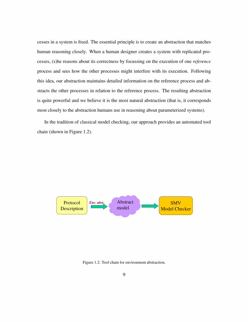
In the tradition of classical model checking, our approach provides an automated tool

chain (shown in Figure 1.2).

ProtocolDescription

Abstractmodel

SMVModel Checker

Env. abst.

Figure 1.2: Tool chain for environment abstraction.

9

1. The behavior of the distributed algorithm/protocol is described in a suitable input

language, cf. Section 3.3 and Section 4.2.

The user’s role ends with inputting the protocol to the verification tool.

1. The environment abstraction tool extracts a finite state model from the protocol de-

scription, and puts the model in SMV format.

2. SMV verifies the specified properties.

We have used this abstraction based method to prove properties of well known cache

coherence systems, mutual exclusion algorithms, and real time protocols.

Typically, handling liveness properties is much harder (theoretically) than handling

safety properties. For instance, the Invisible Invariants method [64] requires significant ad-

ditional work before it can handle liveness properties and the Indexed Predicates method [52;

53] cannot handle liveness properties at all. Informally, this is because verification of

safety properties depends only on the reachable set of states, whereas verification of live-

ness properties depends also on the order in which the various states are reached. Ranking

functions are needed to argue that desirable states are eventually reached. Finding such

ranking functions is typically a non-trivial task.

In contrast, extending our method to handle liveness is very simple. Since our abstract

model simulates the execution of one single process in precise detail and consequently,

liveness properties of a single process are easy to reason about. We only need to rule out

spurious loops introduced by the abstraction.

10

Importantly, other model checking based approaches to parameterized verification

make the atomicity assumption while handling parameterized protocols. The atomicity

assumption in essence states that, in a distributed system with several components, any

component can know (or rather read) the state of all the other components instantaneously.

This is quite unrealistic and simplifies a distributed protocol significantly. In this thesis,

we describe a simple extension to remove the atomicity assumption. Note that the term

atomicity is used in a different sense from the classical usage in distributed computing lit-

erature. In the latter usage, atomicity is used to qualify a single read or write operation. An

atomic read or write operation is one which happens in an atomic time unit and thus, no

other operation can interfere with its execution. Atomicity, as used in this thesis, qualifies

a set of read/write operations.

The idea of looking at a system from the point of view of a reference process can be

carried over into other settings as well. We consider systems with replicated processes

which are arranged at the nodes of an underlying network graph. The processes commu-

nicate by passing tokens among themselves. If we are interested in checking two-process

properties of such a system, we can show that it is enough to consider how the system

looks from the point of view of pairs of processes. This result lets us decompose the ver-

ification problem of a system with a large network graph into verification of a collection

of systems with small, constant sized network graphs. This network decomposition result

lays the ground for reasoning about systems with network graphs and richer inter-process

communication (such as complex leader election protocols).

11

1.1.2 Thesis Outline

The outline for the rest of the thesis is as follows. In the next chapter we present environ-

ment abstraction in general terms and derive its mathematical properties. We show that

environment abstraction is sound for indexed temporal logic specifications in a very gen-

eral framework, and discuss the relationship of our method to counter abstraction, canon-

ical abstraction, and predicate abstraction. This chapter lays the foundation for our work

on verification of parameterized systems with replicated processes. The same chapter also

describes extensions to environment abstraction and considers some of the issues involved

in applying this abstraction method to practical systems.

State-of-the-art architectures crucially rely on cache coherence protocols for increased

performance. These protocols are extremely intricate and, usually, several processors run

these protocols concurrently. Thus, ensuring the correctness of such protocols is a chal-

lenging problem and formal verification techniques are indispensable. Since the number

of processors executing the cache protocol can vary, cache coherence verification is a clas-

sical example of the parameterized verification problem. In Chapter 3, we show how to

apply environment abstraction for verifying cache coherence protocols. We first propose

a simple programming language that allows us to model cache protocols at an algorithmic

level. We then describe the precise abstract state space used in abstracting cache protocols.

Environment abstraction as presented in Chapter 2 talks only about the general structure

of the abstract state space. The precise form of the abstract states depends on the class of

systems under consideration. Chapter 3 also deals with the crucial issue of how exactly

we compute the abstract model. We have applied this method to verify safety properties of

12

several cache coherence protocols, including several variants of GERMAN’s protocol and

a modified version of the FLASH protocol. The language constructs used in describing

cache coherence protocols are quite simple so that the essential principle behind the com-

putation of the abstract model is easy to understand. It is for this reason that we consider

cache coherence protocols as the first example.

In Chapter 4, we show how environment abstraction can be applied to mutual ex-

clusion protocols, which exhibit complex inter-process communication. As with cache

coherence protocols, we first describe a simple programming language that allows us to

describe mutual exclusion protocols at an algorithmic level. The precise form of the ab-

stract states is then described, followed by a section on how to compute the abstract model.

We demonstrate the power of our approach by verifying Lamport’s Bakery algorithm and

Szymanski’s mutual exclusion protocol. Note that in Chapter 4, we verify mutual exclu-

sion protocols under the atomicity assumption.

In Chapter 5, we show how to verify mutual exclusion protocols without the atomicity

assumption. The atomicity assumption, which says that any component can know the

state of all the other components instantaneously, significantly reduces the complexity of a

protocol. To handle protocols in full generality, without the atomicity assumption, we need

to keep track of history information. We introduce monitor processes for this purpose and

show how we can apply environment abstraction in presence of these monitor processes.

In Chapter 6, we consider a different system model, namely systems built around net-

work graphs. For example, in routing protocols, the underlying topology of the system

plays a crucial role. Similarly, in many wireless applications, the system performance de-

13

pends on how the different wireless entities are connected. Formal verification research

has only now begun to address the problem of verifying these systems with complex net-

work graphs. As a first step towards this larger problem, we consider systems consisting

of a collection of identical processes arranged on the nodes of a network graph with very

limited communication between the processes. We describe a new method to verify such

networks of homogeneous processes that communicate by token passing. Given an arbi-

trary network graph and an indexed LTL \ X property, we show how to decompose the

network graph into multiple constant size networks, thereby reducing one model checking

call on a large network to several calls on small networks. We thus obtain cut-offs for

arbitrary classes of networks, adding to previous work by Emerson and Namjoshi on the

ring topology [37]. Our results on LTL \ X are complemented by a negative result that

precludes the existence of reductions for CTL \X on general networks.

The last chapter concludes this thesis with a summary of contributions and possible

extensions to the work presented here. We also discuss some of the outstanding challenges

in parameterized verification.

14

Chapter 2

Environment Abstraction

2.1 Introduction

When a human engineer designs a hardware or software system, the correctness of the

system, naturally, is among the main concerns of the designer. Although the reasoning

of the designer is usually not available to the verification engineer in terms of assertions

or proofs, the reasons for correctness are often reflected in the way a program is written.

Knowledge of these implicit design principles can be systematically exploited for the con-

struction of abstract models. For example, it is natural for us to assume that control flow

conditions yield important predicates for reasoning about software, and that polygons are

good approximations of numeric data that are human generated. Thus, the presence of

a human engineer renders the analysis of hardware and software very different from the

analysis of systems in physics, chemistry, or biology.

15

To pinpoint this difference, consider an example frequently discussed in the history of

science, namely the Ptolemaic system in which the planet earth is surrounded by the sun.

The persistance of Ptolemy’s viewpoint over many centuries shows the intuitive reasoning

which the human mind applies to complex systems: we tend to imagine systems with the

human observer in the center. While a Ptolemaic viewpoint is known to be wrong (or,

more precisely, infeasible) in physics, it naturally appears in the systems we construct.

Consequently, the Ptolemaic viewpoint yields a natural abstraction principle for computer

systems.

In this chapter, we explore a Ptolemaic viewpoint of concurrent systems to devise

an abstraction method for concurrent systems with replicated processes which we call

environment abstraction. Our systems are parameterized, i.e., the number of processes

is a parameter, and all processes execute the same program. We write P(K) to denote a

system with K processes 1. We argue that during the construction of such a system, the

programmer naturally imagines him/herself to be in the position of one reference process,

around which the other processes – which constitute the environment – evolve. Thus, in

many cases, an abstract model that describes the system from the viewpoint of a reference

process contains sufficient information to reason about specifications of interest.

The goal of environment abstraction is to put this intuition into a formal framework. In

environment abstraction, an abstract state is a description of a concrete system state from

the point of view of a single reference process and its environment. The properties of the

reference process are computed as if the process were chosen without loss of generality.

Thus, verification results about the reference process generalize to all processes in the

1We will later also consider a finite number of non-replicated processes in addition.

16

system.

From a practical perspective, environment abstraction shares many properties with

predicate abstraction as used in SLAM [4], BLAST [47], and MAGIC [19]:

• Environment abstraction computes a finite-state abstract model on which a stan-

dard model checker can verify a property. To verify an indexed temporal property

∀x.φ(x) on all parameterized models P(K), K ≥ 1, the model checker just needs

to verify the quantifier-free property φ(x) on a single abstract model PA which

interprets the variable x. The model PA is obtained by a variation of existential

abstraction that quantifies over the parameter K and the index variable x.

• Instead of computing the precise abstract model, environment abstraction over-

approximates the abstract model. To this end, each statement of the concurrent

program is approximated separately using decision procedures. Thus, similar to

SLAM, BLAST, MAGIC, the abstract model used in the verification is an over-

approximation of PA.

The aim of this chapter is to describe environment abstraction from first principles.

We derive environment abstraction from a few simple logical principles, and show its

soundness for a large class of indexed ACTL? properties. In addition, we put the method

in perspective to other abstraction approaches such as Indexed Predicates, and TVLA’s

Canonical Abstraction.

17

2.2 A Generic Framework for Environment Abstraction

We consider parameterized concurrent systems P(K), where the parameter K > 1 de-

notes the number of replicated processes. The processes are distinguished by unique in-

dices in 1, . . . , K which serve as process ids. Each process executes the same program

which has access to its process id. We do not make any specific assumptions about the

processes, in particular we do not require them to be finite state processes.

Consider a systemP(K) with a set SK of states. Each state s ∈ SK contains the whole

state information for each of the K concurrent processes, i.e., s is a vector

〈s1, . . . , sK〉

Technically, P(K) is a Kripke structure (SK , IK, RK, LK) where IK is the set of initial

states and RK is the transition relation. We will discuss the labeling LK for the states in

SK below.

Remark 1. While we consider systems composed solely of replicated processes, sys-

tems with a constant number of non-replicated processes, in addition to a set of replicated

processes, can also be similarly handled. For such systems, each state is of the form

〈s1, . . . , sK, t〉 where t is the combined state of all non-replicated components. With this

minor change, the treatment presented below can be carried as is to this modified setting

as well.

Process Properties. We will describe properties of P(K) using formulas with one free

index variable x which denotes the index of a process. We will call such formulas process

18

properties, as they may or may not hold true for a process in a given state. For a process

property φ(x), we write

s |= φ(c)

to express that in state s, process c has property φ. We assume that for each state s and

process c, we have either s |= φ(c) or s |= ¬φ(c).

Example 2.2.1. The following statements are sample process properties:

• “Process x has program counter position 5.”

We will express this fact by the formula pc[x] = 5. We may use this process property

in all systems where the processes have a variable pc.

• “There exists a process y 6= x where pc[y] = 5.”

This property is expressed by the quantified formula ∃y 6= x.pc[y] = 5. Note that in

this formula, only variable x is free. Intuitively, this property means that a process

in the environment of x has program counter position 5. We shall therefore write

5 ∈ env(x) to express this property.

• “Process x has program counter position 5, and there exist two other processes

t1 and t2 in program counter position 1 such that the data variable d satisfies

d[x] < d[t1] = d[t2].”

This property, too, can be expressed easily with two quantifiers and one free variable

x as shown below

∃t1, t2. t1 6= t2 ∧ x /∈ t1, t2 ∧ pc[x] = 5 ∧ pc[t1] = 1

∧pc[t2] = 1 ∧ d[x] < d[t1] ∧ d[t1] = d[t2]

19

Note that the labels discussed in the first two items are highly relevant in our applica-

tions and will be discussed below in detail.

Labels and Descriptions. In environment abstraction, we distinguish two sets of process

properties that we use for different purposes:

(a) Labels. A label is a process property l(x) that we use in a specification. The set

of all labels is denoted by L. For example, for l(x) = (pc[x] = 10), we may write

∀x.AG ¬(pc[x] = 10) to denote that no process reaches program counter 10. For a

process c, a c-label is an instantiated formula l(c) where l(x) ∈ L. We write L(c) to

denote the set of c-labels.

In the Kripke structure P(K), a state s has a label l(c), if s |= l(c), i.e.,

LK(s) = l(c) : s |= l(c), c ∈ [1..K].

(b) Descriptions. A description is a process property ∆(x) which typically describes

not only the process, but also its environment, as in the second and the third items

of Example 2.2.1. The set of all descriptions D is our abstract state space.

Intuitively, an abstract state ∆(x) ∈ D is an abstraction of a concrete state s if there

exists a concrete process c which has property ∆, i.e., if s |= ∆(c). For example,

the description pc[x] = 5 represents all states s which have a process c whose pc

variable equals 5. In our applications, the descriptions will usually be relatively

large and intricate formulas.

Remark 2. Note that our process properties contain a free index variable x. While the

name of the free index variable is immaterial, we have chosen to call it x as it makes the

20

presentation less cluttered. We also use x in other places, for example, in single index

formulas ∀x.Φ(x). The usage should be clear from the context.

Soundness Requirements for Labels and Descriptions. We will need two require-

ments on the set D of descriptions and the set L of labels to make them useful as building

blocks for the abstract model:

1. Coverage. For each system P(K),K ≥ 2, each state s in SK and each process c

there is some description ∆(x) ∈ D which describes the properties of c, i.e.,

s |= ∆(c).

The coverage property means that every concrete situation is reflected by some ab-

stract state.

2. Congruence. For each description ∆(x) ∈ D and each label l(x) ∈ L it holds that

either

∆(x)→ l(x)

or

∆(x)→ ¬l(x).

In other words, the descriptions in D contain enough information about a process to

conclude whether a label holds true for this process or not.

The congruence property enables us to give natural labels to each state of the abstract

system: An abstract state ∆(x) has the label l(x) if ∆(x)→ l(x).

21

2.2.1 Description of the Abstract System PA.

Given two sets D and L of descriptions and labels that satisfy the coverage and congru-

ence criteria, the abstract system PA is a Kripke structure

〈D, IA, RA, LA〉

where each ∆(x) ∈ D has a label l(x) ∈ L if ∆(x) → l(x), i.e., LA(∆(x)) = l(x) :

∆(x) → l(c). Before we describe IA and RA, we can already state the following lemma

about preservation of labels.

Lemma 2.2.2. Suppose that s |= ∆(c). Then the following are equivalent:

(i) The concrete state s has label l(c).

(ii) The abstract state ∆(x) has label l(x).

Proof. Assume that (i) but not (ii). Then by the congruence property, we have ∆(x) →

¬l(x). Together with the assumption s |= ∆(c) of the lemma, we conclude that s |= ¬l(c),

which contradicts (i). The converse implication is trivial.

Note that the proof of the lemma requires the congruence property.

This motivates the following abstraction function:

Definition 2.2.3. Given a concrete state s and a process c, the abstraction of s with refer-

ence process c is given by the set

αc(s) = ∆(x) ∈ D : s |= ∆(c).

22

Note the following remarks on this definition:

• The coverage requirement guarantees that αc(s) is always non-empty.

• If the ∆(x) are mutually exclusive, then αc(s) always contains exactly one descrip-

tion ∆(x).

• Two processes c and d of the same state s will in general give rise to different ab-

stractions, i.e., αc(s) = αd(s) is in general not true.

Remark 3. In our application of environment abstraction to various distributed protocols,

it is usually the case that the abstract descriptions ∆(x)’s are mutually exclusive. Thus,

given a state s and reference process c, αc(s) will contain exactly one abstract description

∆(x). In such cases, we simply write αc(s) = ∆(x).

Now we define the transition relation of the abstract system by a variation of existential

abstraction: RA contains a transition between ∆1(x) and ∆2(x) if there exists a concrete

system P(K), two states s1, s2 and a process r such that

1. ∆1(x) ∈ αr(s1),

2. ∆2(x) ∈ αr(s2), and

3. there is a transition from s1 to s2 in P(K), i.e., (s1, s2) ∈ RK .

We note three important properties of this definition:

• We existentially quantify over K, s1, s2, and r. This is different from standard

existential abstraction where we only quantify over s1 and s2. For fixed K and r,

our definition is equivalent to existential abstraction.

23

• Both abstractions ∆1 and ∆2 use the same process r. Thus, the point of view of the

abstraction is not changed in the transition.

• The process that actually makes the transition can be any process in P(K), it does

not have to be r.

Finally, the set IA of abstract initial states is the union of the abstractions of concrete

states, i.e., ∆(x) ∈ IA if there exists a system P(K) with state s ∈ IK and process r such

that ∆(x) ∈ αr(s).

To summarize, PA is a Kripke structure (D, IA, RA, LA) such that the set of abstract

descriptions D satisfies the congruence and closure conditions with respect to the set of

labels L and the transition relation RA is defined in an existential fashion.

Remark 4. It will be convenient later on to represent the abstract descriptions as tuples.

For example, if the abstract descriptions were all of the form

±P1(x) ∧ . . .± PT (x), T > 1

where P1(x), . . . , PT (x) are some process properties and ±Pi(x) indicates that property

Pi(x) can appear negated or unnegated, then we can represent an abstract description ∆(x)

as a tuple

〈p1, . . . , pT 〉

where pi = 1 ⇔ ∆(x) ⇒ Pi(x). That is, the value of each bit pi reflects the polarity of

the corresponding predicate Pi(x) in ∆(x).

24

Single-Indexed Specifications and Soundness of Environment Abstraction. We con-

sider an indexed temporal specification language where specifications have the form

∀x.φ(x).

Here, φ(x) is an ACTL? formula whose atomic formulas are labels in L. We say that

P(K) |= ∀x.φ(x) if for all c ∈ 1 . . .K we have P(K) |= φ(c).

Despite the single index, this specification language is powerful, because the labels in

L can talk about other processes. For example, using the label 5 ∈ env(x) from Exam-

ple 2.2.1 above, we can express mutual exclusion by the formula

∀x.AG (pc[x] = 5)→ ¬(5 ∈ env(x))

as well as many other properties. For a more thorough discussion of the expressive power

of this language, see Section 2.4. In Section 2.5.1 we will also consider abstractions with

multiple reference processes for specifications with multiple indices.

For environment abstractions with L and D that satisfy coverage and congruence, we

have the following general soundness theorem.

Theorem 2.2.4 (Soundness of Environment Abstraction). Let P(K) be a parameter-

ized system andPA be its abstraction as described above. Then for single indexedACTL?

specifications ∀x.φ(x) the following holds:

PA |= φ(x) implies ∀K.P(K) |= ∀x.φ(x).

25

2.3 Soundness

We will now give a proof of correctness for Theorem 2.2.4. Before we give the proof

of the soundness theorem we introduce some notation to simplify later proofs.

2.3.1 Simulation Modulo Renaming

Given a fixed process c, we write Pc(K) to denote the Kripke structure obtained from

P(K) where LK is restricted to only those labels which refer to process c. Thus, Pc(K) is

labeled only with c-labels.

Fact 1. Let c be a process in P(K) and φ(x) be a temporal formula over atomic labels

from L. Then

P(K) |= φ(c) if and only if Pc(K) |= φ(c).

This follows directly from the fact that the truth of φ(c) depends only on c-labels.

Our soundness proofs will require a simple variation of the classical abstraction the-

orem [23]. Recall that the classical abstraction theorem for ACTL∗ says that for ACTL∗

specifications φ and two Kripke structures K1 and K2 it holds that K1 K2 and K1 |= φ

together imply K2 |= φ. That is, if K1 simulates K2 then any ACTL∗ property satisfied

by K1 is also satisfied by K2.

Definition 2.3.1 (Simulation Modulo Renaming). LetK be a Kripke structure, and c and

d be processes. Then K[c/d] denotes the Kripke structure obtained from K by replacing

26

each label of the form l(c) by l(d). Simulation modulo renamingc/d is defined as follows:

K1 c/d K2 iff K1[c/d] K2.

Then c/d gives rise to a simple variation of the classical abstraction theorem:

Fact 2 (Abstraction Theorem Modulo Renaming). Let φ(x) be a temporal formula over

atomic labels from L, and let K1, K2 be Kripke structures which are labelled only with

c1-labels and c2-labels respectively.

If K2 c2/c1 K1 and K1 |= φ(c1), then K2 |= φ(c2).

Proof. First note that K2 |= φ(c2) is equivalent to K2[c2/c1] |= φ(c1): if the labels in the

Kripke structure and the atomic propositions in the specification are consistently renamed,

then the satisfaction relation does not change.

Thus, given that K2 c2/c1 K1 and K1 |= φ(c1), it is enough to show that K2[c2/c1] |=

φ(c1) . By the definition of c/d, K2 c2/c1 K1 iff K2[c2/c1] K1 and by the classi-

cal abstraction theorem [23], K1 |= φ(c1) implies K2[c2/c1] |= φ(c1). This proves the

abstraction theorem.

2.3.2 Proof of Soundness

We will show that environment abstraction preserves indexed properties of the form

∀x.φ(x) where φ(x) is an ACTL? formula over atomic labels from L.

Step 1: Reduction to Simulation. Formally, we have to show that

27

PA |= φ(x) implies ∀K.P(K) |= ∀x.φ(x).

By the semantics of our specification language, this is equivalent to saying that for all

K > 1,

PA |= φ(x) implies ∀c ∈ [1..K].P(K) |= φ(c).

Thus, we need to show that for all K > 1 and all processes c ∈ [1..K]

PA |= φ(x) implies P(K) |= φ(c).

Recall that Pc(K) is the Kripke structure obtained from P(K) that contains only c-labels.

By Fact 1 we know that P(K) |= φ(c) iff Pc(K) |= φ(c). Thus, we need to show that for

all K > 1 and for all c ∈ [1..K]

PA |= φ(x) implies Pc(K) |= φ(c).

Now, by the abstraction theorem modulo renaming (Fact 2), it suffices to show that

Pc(K) c/x PA for all K and c ∈ [1..K]

where c/x denotes simulation modulo renaming as defined previously.

We will now prove these simulations.

Step 2: Proof of Simulation. We will now show how to establish the simulation relation

Pc(K) c/x PA between Pc(K) and PA for all K > 1 and c ∈ [1..K]. To this end, for

each K and c, we will construct an intermediate abstract system PAc,K such that

Pc(K) c/x PAc,K (Simulation 1)

and

28

PAc,K P

A. (Simulation 2)

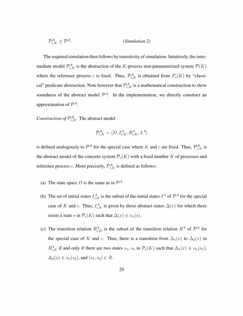
The required simulation then follows by transitivity of simulation. Intuitively, the inter-

mediate model PAc,K is the abstraction of the K-process non-parameterized system P(K)

where the reference process c is fixed. Thus, PAc,K is obtained from Pc(K) by “classi-

cal” predicate abstraction. Note however that PAc,K is a mathematical construction to show

soundness of the abstract model PA. In the implementation, we directly construct an

approximation of PA.

Construction of PAc,K. The abstract model

PAc,K = 〈D, IAc,K, R

Ac,K, L

A〉

is defined analogously to PA for the special case where K and c are fixed. Thus, PAc,K is

the abstract model of the concrete system Pc(K) with a fixed number K of processes and

reference process c. More precisely, PAc,K is defined as follows:

(a) The state space D is the same as in PA.

(b) The set of initial states IAc,K is the subset of the initial states IA of PA for the special

case of K and c. Thus, IAc,K is given by those abstract states ∆(x) for which there

exists a state s in Pc(K) such that ∆(x) ∈ αc(s).

(c) The transition relation RAc,K is the subset of the transition relation RA of PA for

the special case of K and c. Thus, there is a transition from ∆1(x) to ∆2(x) in

RAc,K if and only if there are two states s1, s2 in Pc(K) such that ∆1(x) ∈ αc(s1),

∆2(x) ∈ αc(s2), and (s1, s2) ∈ R.

29

(d) The labeling function LA is the same as in PA.

Proof of Simulation 1. We need to show that Pc(K) c/x PAc,K, which by definition of

c/x is equivalent to

Pc(K)[c/x] PAc,K.

Consider the structure Pc(K)[c/x]. This is just the K-process system P(K) restricted

to the labels for process c, but because of the renaming the labels have the form l(x) instead

of l(c). Thus, the labels of Pc(K)[c/x] are taken from the set L. Note that the labels of the

abstract system PA are also taken from the set L. The proof idea below is similar to the

construction of a simulation relation for existential abstraction.

Consider the relation

I = 〈s,∆(x)〉 : s |= ∆(c), s ∈ SK ,∆(x) ∈ D.

We claim that I is a simulation relation between Pc(K)[c/x] and PAc,K:

1. Lemma 1 together with the renaming of c to x guarantees that for every tuple

〈s,∆(x)〉 ∈ I, the states s and ∆(x) have the same labels.

2. Consider a tuple 〈s,∆(x)〉 ∈ I. Assume that s has a successor state s′, i.e., (s, s′) ∈

RK . We need to show that there exists an abstract state ∆′(x) such that

(i) (∆(x),∆′(x)) ∈ RAc,K , and

(ii) 〈s′,∆′(x)〉 ∈ I.

30

To find such a ∆′(x), consider the abstraction αc(s′) of s′, and choose some descrip-

tion Γ(x) ∈ αc(s′). By the coverage condition, αc(s′) is non-empty.

We will show by contradiction that each such Γ(x) fulfills the properties (i) and (ii)

menitioned above.

Property (i) Assume that Γ(x) does not fulfill property (i), i.e., (∆(x),Γ(x)) 6∈

RAc,K . Then for all states s1 and s2 it must hold that whenever ∆(x) ∈ αc(s1)

and Γ(x) ∈ αc(s2) that there is no transition between s1 and s2. On the other

hand, we assumed above that ∆(x) ∈ αc(s), Γ(x) ∈ αc(s′) and there is a

transition from s to s′. Hence we have a contradiction.

Property (ii) Assume now that Γ(x) does not fulfill property (ii), i.e, 〈s′,Γ(x)〉 6∈

I. By the definition of I, this means that s′ 6|= Γ(c), and thus, Γ(c) 6∈ αc(s′).

This gives us the required contradiction.

Thus, ∆′(x) can be chosen from among the descriptions in αc(s′).

3. Finally, the coverage property guarantees that for every initial state s ∈ IK there

exists some ∆(x) ∈ IAc,K s.t. 〈s,∆(x)〉 ∈ I.

Proof of Simulation 2. By construction, IAc,K ⊆ IA and RAc,K ⊆ RA. Therefore, PA is an

over-approximation of PAc,K , and the simulation follows.

Remark 5. Note that the coverage and congruence requirements for D and L are used

in crucial parts of Simulation 1 in the soundness proof. Congruence is used in the proof

of Lemma 2.2.2 which gives us property 1 of Simulation 1. Property 2 of Simulation 1

31

requires coverage to make sure that αc(s′) is non-empty. Property 3 of Simulation 1 also

requires coverage to ensure the existence of an abstract initial state.

Remark 6. In the formulation above, we have not assumed that processes inP(K) execute

synchronously or asynchronously. That is, our definitions are not affected by how the

system evolves. We only assume that there is a global transition relation for P(K). Thus,

results described above hold whether the processes in P(K) execute synchrounously or

asynchronously. This fact will allow us to later augment P(K) by adding synchronously

executing monitor processes.

2.4 Trade-Off between Expressive Labels and Index Vari-

ables

In this section we argue why a well-chosen set of labels L makes it often possible to

use a single index variable. The Ptolemaic system view explains why we seldom find more

than two indices in practical specifications: when we specify a system, we tend to track

properties the reference process has in relation to other processes out there, one at a time.

Thus, two-indexed specifications of the form

∀x, y. x 6= y → φ(x, y)

often suffice to express the specifications of interest. Properties involving three processes

at a time are typically complicated, as we need to consider a triangle of processes and their

relationships.

32

In our work on verifying mutual exclusion and cache coherence protocols, we used

two kinds of labels (see also Example 2.2.1):

• pc[x] = L and

• L ∈ env(x) which semantically stands for ∃y 6= x.pc[y] = L.

Note that the label pc[x] = L refers only to process x whereas L ∈ env(x) also refers

to the environment of x using a hidden quantification. This hidden quantification in the

environment label gives surprising power to single-indexed specifications.

To see this, consider the standard mutual exclusion property. The classical way to

specify mutual exclusion is expressed in a formula such as

∀x, y.x 6= y → AG (pc[x] = 5)→ (pc[y] 6= 5).

It is easy to see that using the label 5 ∈ env(x), we can express this specification by the

logically equivalent single-indexed formula

∀x.AG (pc[x] = 5)→ ¬(∃y 6= x.pc[y] = 5).

which is in turn equivalent to

∀x.AG (pc[x] = 5)→ ¬(5 ∈ env(x))

The difference between the three formulas is that in the first specification the index

quantifiers are in prenex form, while in the second and third formula, the quantifier for y

has been distributed inside the formula, and is hidden in the label 5 ∈ env(x). Again, the

33

Ptolemaic viewpoint explains why such situations are likely to happen: in many specifi-

cations, we consider our process over time (i.e., using a temporal logic specification), but

only at the individual time points we evaluate its relationship to other processes. Thus, a

time-local quantification suffices.

The interplay between labels and index variables gives rise to interesting logical con-

siderations that we will discuss briefly now.

Distributive Fragments of CTL and LTL. It is natural to ask when a double-indexed

specification can be translated into a single-indexed specification as in the example above.

Somewhat surprisingly, this question is related to previous work on temporal logic query

languages [73; 74; 75]. A temporal logic query is a formula γ with one occurrence of a

distinguished atomic subformula “?” (called a placeholder). Given γ and a formula ψ, we

write γ[ψ] to denote the formula obtained by replacing ? with ψ. In [73; 74; 75], syntactic

characterizations for CTL and LTL queries with the distributivity property

γ[ψ1 ∧ ψ2]↔ γ[ψ1] ∧ γ[ψ2].

are described. A template grammar for the distributive fragment of LTL is given in the

appendix of [74].

The prototypical example of a distributive query is AG?, and we have seen above

that for AG properties, we can translate double indexed properties into single-indexed

properties. As argued above, this translation actually amounts to distributing one universal

quantifier inside the temporal formula.

Such a translation is possible for all specifications which are distributive with respect

34

to one index variable: consider a double-indexed specification ∀x, y. x 6= y → φ(x, y)

where all occurrences of y in φ are located in a subformula θ(x, y) of φ. Then we can

write φ as a query γ[θ]. Now suppose that γ is distributive. On each finite P(K), the

universal quantification reduces to a conjunction, i.e.,

P(K) |= ∀x, y. x 6= y → γ[θ(x, y)] iff P(K) |= ∀x.∧

1≤c≤K,c6=x

γ[θ(x, c)]

which by distributivity of γ is equivalent to

P(K) |= ∀x. γ

[ ∧

1≤c≤K,i6=x

θ(x, c)

]

and thus to

P(K) |= ∀x. γ [ ∀y.x 6= y → θ(x, c) ] .

For a suitable label l(x) := ∀y. x 6= y → θ(x, y) this can be written as

P(K) |= ∀x. γ[l(x)].

For the important special case where θ(x, y) has the form pc[y] = L, this is equivalent to

P(K) |= ∀x. γ[L 6∈ env(x)].

While the characterization of distributive queries gives us a good understanding about

the scope of single-indexed specifications, it is clear that not all two-indexed specifications

can be rewritten with a single index. Consider, for example, the formula

∀x, y.x 6= y → AF(pc[x] = 5 ∧ pc[y] = 5).

Here it is evidently not possible to move the quantifier inside. This can also be derived

from the characterization in [74]. Consequently, this specification cannot be expressed

with a single index.

35

In Section 2.5.1 we will show how to extend environment abstraction to multiple ref-

erence processes. Of course, having more reference processes will, in general, make the

abstract model larger, and, thus, harder to analyze. This motivates the following approach

to deal with two-indexed specifications σ:

1. Using the grammar characterizations of distributive queries, determine whether σ

can be written with a single index.

2. Otherwise, use an abstraction with two reference processes, as described in Sec-

tion 2.5.1.

2.5 Extending Environment Abstraction

In this section, we will describe a few easy extensions to environment abstraction.

2.5.1 Multiple Reference Processes

In the preceding sections, we focused on a framework for single-indexed specifications

of the form ∀x.φ(x). Extending this framework to two reference processes is simple –

essentially, we need to replace the free variable x in the process properties by a pair x, y,

and carry this modification through all definitions and proofs. The generalization to more

indices is straightforward, and left to the reader.

36

For the set D of descriptions, we will now use descriptions of the form ∆(x, y) which

capture the state of two reference processes x, y and the environment around them. Thus,

we can track the mutual relationship of two processes in greater detail. Similarly, we can

extend the set of labels. The set L of labels is partitioned into unary labels L1 of the form

l(x) and binary labels L2 of the form l(x, y). Note that, in practice, the single-indexed

labels will usually suffice. A state s of system P(K) is labeled with l(c) if and only if

s |= l(c). State s is labeled with l(c, d) if and only if s |= l(c, d).

The coverage and congruence requirements are generalized analogously:

1. Coverage. For each system P(K), each state s in P(K) and any two processes c, d

there is some description ∆(x, y) ∈ D which describes the properties of c, d, i.e.,

s |= ∆(c, d).

2. Congruence. For each description ∆(x, y) ∈ D and each label l(x, y) ∈ L2 it holds

that either ∆(x, y)→ l(x, y) or ∆(x, y)→ ¬l(x, y). An analogous condition holds

for labels in L1.

Thus, we obtain a natural definition of the abstraction mapping:

Definition 2.5.1. Given a concrete state s and two processes c and d, the abstraction of s

with reference processes c and d is given by the set

αc,d(s) = ∆(x, y) ∈ D : s |= ∆(c, d).

The construction of the abstract model is analogous to the single index case. To in-

dicate the number of reference processes in the abstract model, we write P A2 for the ab-

37

stract model with two reference processes. Analogously to the single-index case, we at-

tach labels to each state of PA2 such that the abstract state ∆(x, y) has label l(x, y) iff

∆(x, y)→ l(x, y).

Theorem 2.5.2 (Soundness of Double-Index Environment Abstraction). Let P(K) be

a parameterized system and PA2 be its abstraction with two reference processes. Then for

double indexed ACTL? specifications ∀x 6= y.φ(x, y) the following holds:

PA2 |= φ(x, y) implies ∀K.P(K) |= ∀x 6= y.φ(x, y).

The environment abstraction principle can be easily extended to incorporate more than

two reference processes. As argued above, it is quite unlikely that a practical verification

problem will require the use of three reference processes.

2.5.2 Adding Monitor Processes

Often times it is necessary to augment a given parameterized system P(K) by adding

non-interfering monitor processes. Monitors are essentially synchronous processes (i.e.,

they execute at every step of P(K)) that maintain history information regarding the pro-

cesses in P(K). Addition of monitors gives more information about the evolution of the

system. Thus, taking monitors into account during abstraction can give us better abstract

models. A typical case where monitors are needed is for handling liveness properties.

As we will see later in Section 4.4, environment abstraction, as described in the earlier

38

sections, is too coarse to handle liveness properties. This is because the abstraction can

introduce spurious loops, which can lead to false negatives. These spurious abstract be-

haviors can be eliminated by augmenting the system P(K) with monitors and abstracting

the augmented system. While the precise details of monitor processes are considered later

in Chapter 4, we will consider here the theoretical basis for adding monitors.

Consider a parameterized system P(K) and assume that we augment it by adding

a collection of identical monitor processes M(1), . . . ,M(K). Each M(i) is exactly the

same as the other monitor processes except for its id. Denote the augmented param-

eterized system by PM(K). The states of PM(K) are given by tuples of the form

sM.= 〈L1, . . . ,LK,M1, . . . ,MK〉 where Li is denotes local state of process P (i) and

Mi denotes the local state of the monitor process M(i).

The results presented in Section 2.2 assume there is only one collection of replicated

process. To make the results of Section 2.2 applicable, we can compose each M(i)

with the corresponding P (i) to create a hybrid process PM(i). The augmented system

PM(K).= 〈SM , IM , RM , LM〉 is a parameterized system with PM(i)’s as the constitut-

ing processes. The set of labels LM is usually the same as the set of labels L of P(K). To

apply environment abstraction to PM(K) we just have to pick the appropriate set of ab-

stract descriptions satisfying the congruence and coverage properties together with labels

in L. Let DM be a collection of abstract descriptions ∆M (x) and αM be the abstraction

mapping from SM to DM such that DM satisfies the coverage and congruence conditions

with respect to the set of labels L.

Define the augmented abstract model PAM in the usual fashion.

39

Definition 2.5.3 (Augmented Abstract Model). The abstract model PAM of a parameter-

ized system PM(K) is defined as the Kripke structure (DM , IAM , R

AM , L

AM) where

• DM is the set of all augmented abstract descriptions

• IAM , the set of initial abstract states, is the set of augmented abstract states sM such

that there exists a concrete initial state sM of a concrete system PM(K), K > 1,

and a process p ∈ [1..K], such that αMp(sM) = sM .

• RAM is defined as follows: There is a transition from abstract state sM1 to abstract

state sM2 if there exist

(i) a concrete system PM(K), K > 1 with a process p

(ii) a concrete transition from concrete state sM1 to sM2

in PM(K)

such that αMp(s1) = sM1 and αMp

(s2) = sM2 .

• ∆M(x) is labeled with l(x) ∈ L if and only if ∆M (x)⇒ l(x).

Corollary 1. Let PM(K) be the augmented parameterized system corresponding to the

parameterized systemP(K). LetPAM be the augmented abstract model as described above.

Then, for any single indexed ACTL∗ specification ∀x.φ(x), where φ(x) is a formula over

labels L, we have

PAM |= φ(x)⇒ ∀K > 1.PM(K) |= ∀x.φ(x)

Proof. This follows simply from Theorem 2.2.4. Note that we are using the fact that

Theorem 2.2.4 holds whether the parameterized systemP(K) executes asynchronously or

not.

40

Since we have assumed that the monitors are non-interfering, PM(K) |= ∀x.φ(x)

implies P(K) |= ∀x.φ(x). Thus

PAM |= φ(x)⇒ ∀K > 1.PM(K) |= ∀x.φ(x)⇒ ∀K > 1.P(K) |= ∀x.φ(x)

Remark 7. Note that the number of monitor processes is exactly the same as the number

of processes. This does not reduce the generality of the results above for the following

reasons: if the number of monitor processes is constant (i.e., independent of K) then they

can be treated as one single non-replicated process. On the other hand if the number

of monitors was a function of K then we can compose a set of monitors and processes

(instead of one monitor and one process) to create composite processes. For example,

suppose we had only K/2 monitors in the system P(K) with K processes. Then we

can compose two processes and one monitor to create a larger composite process P 2M(i)

and the augmented parameterized system is composed of K/2 such composite processes.

Thus, our results will still be applicable.

2.6 Example of Environment Abstraction

We have thus far described environment abstraction in its most general terms. We have

not indicated what descriptions to choose or what labels to use beyond specifying their

general forms. In the following, we discuss, using an example, some of these issues which

let us apply this abstraction method to practical systems.

41

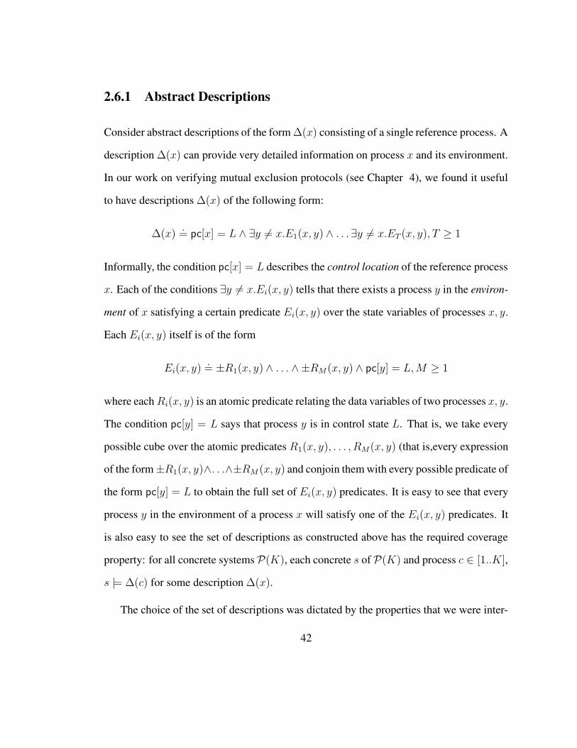
2.6.1 Abstract Descriptions

Consider abstract descriptions of the form ∆(x) consisting of a single reference process. A

description ∆(x) can provide very detailed information on process x and its environment.

In our work on verifying mutual exclusion protocols (see Chapter 4), we found it useful

to have descriptions ∆(x) of the following form:

∆(x).= pc[x] = L ∧ ∃y 6= x.E1(x, y) ∧ . . .∃y 6= x.ET (x, y), T ≥ 1

Informally, the condition pc[x] = L describes the control location of the reference process

x. Each of the conditions ∃y 6= x.Ei(x, y) tells that there exists a process y in the environ-

ment of x satisfying a certain predicate Ei(x, y) over the state variables of processes x, y.

Each Ei(x, y) itself is of the form

Ei(x, y).= ±R1(x, y) ∧ . . . ∧ ±RM (x, y) ∧ pc[y] = L,M ≥ 1

where eachRi(x, y) is an atomic predicate relating the data variables of two processes x, y.

The condition pc[y] = L says that process y is in control state L. That is, we take every

possible cube over the atomic predicates R1(x, y), . . . , RM(x, y) (that is,every expression

of the form±R1(x, y)∧. . .∧±RM (x, y) and conjoin them with every possible predicate of

the form pc[y] = L to obtain the full set of Ei(x, y) predicates. It is easy to see that every

process y in the environment of a process x will satisfy one of the Ei(x, y) predicates. It

is also easy to see the set of descriptions as constructed above has the required coverage

property: for all concrete systemsP(K), each concrete s of P(K) and process c ∈ [1..K],

s |= ∆(c) for some description ∆(x).

The choice of the set of descriptions was dictated by the properties that we were inter-

42

ested in verifying, namely, two index safety properties of the form

∀x, y.x 6= y ∧ (pc[x] = crit⇒ ¬(pc[y] = crit)

As discussed earlier, this property can be equivalently written as

∀x.(pc[x] = crit⇒ ¬(∃y 6= x.pc[y] = crit))

Thus, the two indexed property is essentially composed of two kinds of labels

• pc[x] = L, and

• ∃y 6= x.pc[y] = L.

Observe first that only x occurs free in both types of labels. Further, each description

∆(x) either implies pc[x] = L or its negation. Similarly, each ∆(x) either implies ∃y 6=

x.pc[y] = L or its negation. Thus, we also have the required congruence property. Thus,

the set of descriptions we chose have both congruence and coverage properties required

by our abstraction framework.

As an aside, if we let ∃k stand for the generalization of the usual existential quantifier

∃ meaning there exist at least k different elements, then our descriptions can be made even

stronger. Instead of the descriptions above we can use

∆(x).= pc[x] = L ∧ ∃ky 6= x.E1(x, y) ∧ . . .∃

ky 6= x.ET (x, y).

Instead of just telling us whether there is a process satisfying Ei(x, y) these descriptions

also tell us whether there are atleast k such processes or not. Note that this is quite close

in spirit to counting abstraction which also counts processes satisfying certain conditions

(though there is no notion of a reference process in counting abstraction).

43

2.7 Related Work

Verification of parameterized systems is well known to be undecidable, see [2; 76].

Nonetheless, many interesting approaches to this problem have been developed over the

years, including the use of symbolic automata-based techniques [1; 10; 12; 51], invari-

ant based techniques [3; 64], predicate abstraction [52], and symmetry [24; 31; 38; 39;

40]. Some of the earliest work on verifying parameterized systems includes the works

by Browne et al [14; 15], German and Sistla [43], and Emerson and Sistla [38]. Pa-

pers that handle systems similar to the parameterized systems considered in this thesis

are [3; 6; 7; 41; 42; 52; 53; 64; 66]. The paper [66] by Pnueli et al., which introduces the

term counter abstraction, inspired our work.

Environment abstraction fits the Abstract Interpretation framework of Cousot and

Cousot [26]. In the Abstract Interpretation framework one studies the effect of a program

in an abstract domain instead of the concrete domain that the program is supposed to

handle. The abstract domain is designed to be sound so that a property that holds in the

abstract domain will also hold in the concrete domain. While this provides a general

methodology, it provides no guidance on what abstract domain to choose. The choice

of the abstract domain to consider is in fact the toughest question facing any Abstract

Interpretation based method.

In the context of verifying software and hardware systems, several different alternatives

have been proposed to construct abstract domains. Any such method must address two

conflicting issues:

44

Generality: The abstract domains must be as widely applicable as possible. It de-

feats the propose of automated and efficient program analysis if the user has to figure

out the abstract domain for each and every program separately. Thus, it is required

that methods for constructing the abstract domains should not be too specific.

Usability: On the other hand, widely applicable but trivial abstract domains can be

constructed quite easily. Such abstract domains are useless in proving interesting

properties of a program under consideration. It is typically the case that the more

widely a method (for constructing abstract domains) is applicable, the less powerful

it is.

In this thesis, we are essentially proposing a new approach for constructing abstract

domains. This approach is applicable to any system that has replicated components. For

such systems, the abstract domain we consider has detailed information on one reference

component and the rest of the components are considered in less detail and in relation

to the reference component. It is our claim that this is the way a human designer thinks

(when designing systems with replicated components), and, hence the abstract domains

constructed according to this pattern will be powerful. It is to be noted that we have not

specified all the details of the abstract domain as they necessarily depends on the specific

class of programs under consideration. But following this general structure, we hope that

filling in the details will be easy.

In the following sections we discuss some of the well known abstraction methods and

how they relate to our work.

45

2.7.1 Predicate abstraction

This method, proposed by Graf and Saidi [70; 72] has, over the years, become one of the

most widely used abstraction mechanisms for handling systems with large or unbounded

state spaces. The basic idea of this approach is to consider the effect of the program on a set

of (carefully chosen) predicates. The abstract domain consists of a set of predicates over

the program variables. Assume that the set of predicates is P .= P1, . . . , Pn. The ab-

stract domain consists of all possible valuations 〈b1, . . . , bn〉 of the predicates P1, . . . , Pn.

Denote the set of concrete states by S and the set of abstract states by S. We can then

define the standard abstraction mapping α from S to abstract states S as follows. For any

concrete state s ∈ S and 〈b1, . . . , bn〉 ∈ S

α(s).= 〈b1, . . . , bn〉 such that each bi = 1 iff s |= Pi.

The corresponding concretization mapping γ from S to 2S is then defined as

γ(〈b1, . . . , bn〉).= s|α(s) = 〈b1, . . . , bn〉

Once the abstraction mapping is defined, the abstract model is described using the well-

known existential definition: given two abstract states s1, s2 there is an abstract transition

from s1 to s2 if there exist two concrete states s1, s2 such that

• α(s1) = s1,

• α(s2) = s2, and

• there is a concrete transition from s1 to s2.

46

It can be shown that the abstract model so defined is a conservative abstraction of the

concrete system [70].

Predicate abstraction is a very general method. The main problem in applying pred-

icate abstraction is in deciding what set of predicates to use. This is an active area of

research and several heuristics are used to discover relevant predicates to use (for example

the CEGAR loop [22]). In contrast, our method does provide a framework for constructing

predicates.

There are some crucial differences between standard predicate abstraction and our

method. Given a fixed set of predicates, each concrete state can map only to one ab-

stract state in usual predicate abstraction. On the other hand, in our abstraction method, a

concrete state can map to multiple abstract states depending on which process is chosen as

the reference process.

Further, in standard predicate abstraction, the predicates typically involve the variables

of the same process/program. In our approach, the predicates span multiple processes and

relate the states of different components in the system. TVLA [71; 80] was the first work

to identify the importance of such predicates and it has been successfully used to verify

various multi-threaded systems and heap properties. We believe the use of predicates re-

lating different processes/components within a system is a natural and powerful extension

of standard predicate abstraction. Such predicates are required if one wants to verify multi

process systems or reason about heap properties.

47

2.7.2 Indexed Predicates

The Indexed Predicates approach was proposed by Lahiri and Bryant [52; 53] to handle

unbounded systems such as those with replicated processes or unbounded data structures.

The invariants of such systems are usually quantified over the parameters and the indices

of the various components of the system. Typically, the scope of the quantifiers contains

complex formulas (which are themselves composed of smaller predicates containing free

index variables). If one were to use standard predicate abstraction, discovering such invari-

ants would involve predicates which are almost as complex as the invariants themselves.

To get around this problem, the Indexed Predicates approach uses simple predicates which

can contain free-index variables and tries to build complex quantified invariants from these

indexed predicates. The invariants discovered using this method contain only universal

quantifiers.

The Indexed Predicates starts with a set of predicates P .= P1, . . . , Pn which can

contain free index variables from a set X . As with standard predicate abstraction, the

abstract state space S is just the set of all possible valuations 〈b1, . . . , bn〉 of the atomic

predicates in P . The abstraction mapping function though is quite different. A concrete

state smaps to an abstract state s .= 〈b1, . . . , bn〉 if for some valuation of the index variables

inX the value of each predicate Pi in P matches the corresponding bi in s. More formally,

let v(X ) denote some valuation of the index variables in X . Then

α(s).= s ∈ S|∃v(X ).(s |=v(X ) Pi ⇔ bi)

where s |=v(X ) Pi means state s satisfies predicate Pi with all the free index variables

occuring in Pi fixed according to the valuation v(X ).

48

Since there are multiple possible valuations for variables in X , a single concrete state

can map to several different abstract states. Note that, in our method a single concrete state

can also map to several different abstract states depending on which process is chosen as

the reference process (the reference process in our method can be modeled as a free index

variable). Thus, the abstraction mapping used in our method and in Indexed Predicates

are essentially the same. But unlike our method, Indexed Predicates method defines a

concretization function for a set of abstract states, not for a single abstract state. The

concretization of a set of abstract states C is the set C of concrete states such that, for all

valuation of the free index variables, every state s ∈ S maps to some state s ∈ S. More

formally, for a set C of abstract states

γ(C).= C ⊆ S|∀s ∈ C.α(s) ⊆ C

The abstract reachability is carried out by defining a reachability function that operates

on sets of abstract states instead of single abstract states. Denote the concrete transition

relation by ρ. Then the abstract reachability function ρ is defined as:

ρ(S).= α(ρ(γ(S)).

Let R, R be the set of concrete and abstract reachable states. Then it can be shown

that [53]

α(R) ⊆ R.

Thus, an over-approximation of the concrete reachable states can be found by doing a

reachability analysis on the abstract model.

49

A crucial difference between our method and Indexed Predicates method is that we can

define a concretization function that operates on individual abstract states instead of sets

of abstract states. In our framework, the concretization function γ is defined as follows.

For an abstract state s

γ(s).= s ∈ S|∃c.αc(s) = s

where c is the reference process.

Because we can talk of concrete states corresponding to each abstract state, we can also

define an abstract transition relation, not just an abstract reachability function operating on

sets of states (as in Indexed Predicates. 2) As a consequence, Indexed predicates method is

not suited for handling liveness properties, which requires an abstract transition relation.

Indexed Predicates method can verify only safety properties. In contrast, our approach can

handle both safety and liveness properties.

In Indexed Predicates, the computation of the abstract reachable states is done symbol-

ically by reducing each step of the reachability analysis to finding solutions of a quantified

CLU formula (CLU logic is a subset of first order logic with uninterpreted functions [18]).

Quantified CLU formulas are then solved by posing them as Boolean SAT problems [17].

Observe that this method of abstract reachability does not really exploit our knowledge of

the concrete transition statements. On the flip side, the systems that Indexed Predicates can

handle is limited in theory only by the availability of solvers for first order logic formulas.

In contrast, in our approach, we consider each statement of the protocol and compute

an over-approximation of all the abstract transitions this can lead to. In doing this, we2As an aside, we believe the Indexed Predicates method can also be generalized to have an abstract

transition relation.

50

are able to exploit our knowledge of the transition statements whereas Indexed Predicates

cannot. This means that, for each type of transition statement, we have to write by hand

an over-approximation for it. We believe this is a novel feature of our approach: the user

has to provide an over-approximation for each type of transition statement in the system.

Since there are limited number of different types of transition statements (in our work on

protocol verification we had around 6 types), this is a fairly easy task.

Another difference between the two approaches is that Indexed Predicates is a general

framework much in the spirit of standard predicate abstraction and TVLA. It provides no

guidance on what predicates to use. This problem is compounded by the fact that, unlike

predicate abstraction, there is no possibility of applying the Counterexample Guided Ab-

straction loop to extract useful predicates. This is because there is no abstract transition

relation in Indexed Predicates and consequently, no notion of an abstract trace. Our ap-

proach, in contrast, does provide a guideline for what predicates to use. Moreover, as we

have an abstract transition relation, automatic predicate discovery guided by counterexam-

ple traces is also possible.

2.7.3 Three Valued Logical Analysis (TVLA)

The TVLA method proposed by Reps et al. [71; 80] is an abstract interpretation based

approach for verifying safety properties of multi-threaded systems, and for doing shape

analysis. This is a widely applicable method that uses the universe of first order logical

structures as the abstract domain. To make verification of unbounded systems possible,

they use the notion of summarization, which is similar to the idea of counting abstraction.

51

The essential idea is to represent the state of a system as a first order structure (called

a configuration) consisting of objects and predicates over these objects. The objects in

the first order structure can be used to represent threads and heap allocated data structures.

The predicates can be used to represent relationships between the objects. For example, the

fact that a pointer p points to thread t can be represented by using a predicate pointsTo(p,t).

Papers on TVLA were the first to observe that predicates spanning or relating multiple

components of a system are essential if we want to reason about multi-threaded systems

and heap properties.

Once a set of relevant predicates have been picked, the mapping from concrete states

to abstract states is straight-forward. There is a one to one mapping from the threads and

other components of the concrete system to the objects in the abstract domain. Further, the

valuations of the different predicates are known from the concrete state being considered.

If the number of threads and other components in the concrete system are bounded then

the number of objects necessary in the abstract domain is also finite.

To handle the case where the concrete system can have an unbounded number of

threads and other components, TVLA uses the notion of summarization which is essen-

tially a form of counting abstraction. Suppose components c1, . . . , cn all satisfy the same

set of unary predicates 3. Then instead of mapping them to different objects o1, . . . , on in

the abstract domain, they are mapped to one abstract object o. Thus, an unbounded num-

ber of concrete components can be summarized using a single abstract object o. Observe

that summarization of o1, . . . , on into one abstract object o introduces uncertainty in the

3TVLA uses binary predicates to specify relationship between different components and unary predicates

to specify properties of a particular component.

52

properties satisfied by o. For instance, suppose object o1 satisfies a certain binary predi-

cate Bin(o1, t) for some fixed arguement t, but the rest of the objects do not. It is not clear

in this case whether o should satisfy Bin(o, t) or not. To deal with situations like these,

TVLA uses three-valued logic (hence the name) instead of the standard two-valued logic.

Thus, a predicate P can take three values 0, 1/2, and 1, where 0, 1 have the usual meaning

and 1/2 denotes that P can have either value.

While summarization of similar objects is a powerful feature that lets TVLA deal with

unbounded systems, it is sometimes necessary to track one object,say o1, separately from

other objects o2, . . . , on even though they may have the same properties. For this sake,

special unary predicates can be used to select some particular object as a special object

and thus track its execution in detail. Such unary predicates used to distinguish individual

objects are called instrumentation predicates.

It might seem that instrumentation predicates can be used to simulate our notion of a

reference process, but that is not the case. The only thing that distinguishes a reference

process from other processes in the system is its id. Thus, if we use instrumentation

predicates to simulate the notion of a reference process, the predicates will have to refer

to the process ids. This means that once a reference process is chosen by instrumentation

predicates it cannot change. But, in our abstraction, the identity of the process that serves

as the reference process may change from transition to transition. Thus, the notion of a

reference process cannot be simulated using instrumentation predicates.

To explore the state space of a given system, TVLA starts with the initial set of ab-

stract configurations each of which corresponds to some concrete initial state. The actions

53

of the concrete system rewrite the abstract configurations into new configurations. TVLA’s

model checker performs on-the-fly model checking by exploring new configurations until

all the configurations are covered. Because of summarization, the set of abstract configura-

tions is bounded, and the explicit exploration of the abstract domain will terminate. Thus,

no abstract model is built up front on which model checking is performed. In contrast, in

our method we build an abstract model up front.

The framework proposed by TVLA is extremely general; essentially any real world

system can be handled by this framework. Consequently, no method for choosing the

predicates can be specified and the central problem in predicate abstraction, namely what

predicates to use, is left unsolved. For the examples considered in [81], the authors man-

ually pick the predicates. In contrast, our method specifies a framework for what type of

predicates to pick. In our case studies, the relevant predicates were constructed just by a

syntactic exploration of the protocol code.

2.7.4 Counter Abstraction

Counter Abstraction is an intuitive method to use on parameterized systems, and it has

been employed by various researchers in different contexts [5; 28; 34; 66]. Pnueli et

al. [66], who coined the term counter abstraction, show how concurrent systems com-

posed of symmetric and finite state processes can be handled automatically. The essential

idea in counter abstraction is to have a counter Ci for each possible local state i of the

processes. Counter Ci then counts the number of processes in state i in a given concrete

system configuration. The counters are typically bounded by a small value so that the ab-

54

stract system consisting of the counters is finite state. Environment abstraction generalizes

counter abstraction since the abstract descriptions ∆(x) can serve as counters. But, in-

stead of counting simply the processes according to their local states, we count processes

according to their local states and according to their relationship to the reference process.

It is the latter feature that lets us handle systems in which each replicated process has

infinite state space.

In a symmetric protocol, the identities of the processes cannot be used in the protocol

code. For instance, a condition of the form

forall j < i. Φ(j)

appearing in the code of process i breaks the symmetry because the process with id 1 will

exhibit different behavior from process with id m > 1 (the condition is trivially true for

process 1 and not so for other processes with ids greater than 1). Most real life systems are

not symmetric, that is, the code for each process can make use of the process id. Thus, the

verification of Szymanski’s protocol in [66] requires manual introduction of new variables.

Our method does not require each process to be finite state nor do we require the processes

to be symmetric.

In [66], the notion of “all-but-one” counter abstraction is described. The idea here is

to apply counter abstraction to all processes except one. By tracking one special process

in detail, they are able to reason about single index liveness properties. It is important to

note the following:

• In a symmetric protocol, any process can be chosen as the special process, it makes

no difference in the abstraction.

55

• Further, the other processes in the system are abstracted (or counted) according to

their local states alone, not based on their relationship to the special process. This is

the crucial difference between our method and counter abstraction.

There are also important differences in how we compute the abstract model and how

the abstract model is computed in [66]. In [66], the abstract model is computed precisely

using symbolic techniques. In contrast, we over-approximate the abstract model by con-

sidering each transition statement of the protocol code.

Another approach that uses, among other things, counter abstraction is the method

proposed by Henzinger et al. [45]. Like “all-but-one” abstraction of Pnueli et al. [66],

Henzinger et al. also track one thread in detail (called the main thread). As with counter

abstraction, the main thread does not serve as a reference process. The other threads in the

system are abstracted independently of the main thread.

2.8 Conclusion

In this chapter we presented the mathematical principles underlying environment ab-

straction. This abstraction framework is designed specifically for systems with replicated

components. Informally, this framework is built around the insight that when we humans

reason about systems with replicated components we focus on one particular component

while considering the other components only abstractly.

In this chapter, we assumed that the replicated components were processes. In general

56

the replicated components can vary. For instance, a memory bank can be treated as a

collection of identical memory cells. Our method can be extended to all these instances as

well.

It is crucial to distinguish two different issues that have been covered in this chapter:

(i) “what abstract state space to consider?” and (ii) “how to build the abstract model?”

or rather, “how to use this abstract state space to accomplish verification?”. In answer

to the first question we propose using an abstract state space of descriptions ∆(x). In

answer to the second question, we propose constructing, up front, an over-approximate

abstract model. It is not necessary for using environment abstraction that we build the

abstract model up front. We can use an explicit state exploration as done by TVLA as

well. However, we think that for protocols, which can usually be expressed using only a

few types of basic constructs, our way of building the abstract model up front is the best

possible choice.

In the next chapter, we instantiate environment abstraction in the context of cache

coherence verification. We will cover all the issues raised in this chapter from descriptions

to computing the abstract model.

57

Chapter 3

Environment Abstraction for

Verification of Cache Coherence

Protocols

3.1 Introduction

The performance advantages of multi-core shared memory architectures have created a

strong industrial trend towards multi-core designs. Such state-of-the-art architectures cru-

cially rely on caching mechanisms for increased performance. The increasing complexity

of such systems is reflected in the intricate cache protocols they employ. As these cache

coherence protocols are inherently parameterized, it is a challenging task to ensure their

correctness by automatic verification methods. In this chapter, we show how to use the

59

environment abstraction to verify directory based cache coherence protocols – the most

widely employed class of cache coherence protocols. We use this abstraction method to

verify the standard safety property of several versions of the GERMAN’s protocol and of

a modified version of the FLASH protocol.

3.1.1 Cache Coherence Protocols

Caching mechanisms are ubiquitous in modern computer systems. Computer systems

usually have several memory banks, each with different latency. To reduce the time needed

to access data items and thus improve the performance, caching mechanisms are used to

store frequently accessed data items in the fastest available memory bank.

Modern processors typically come with several levels of caches. A cache is a small

memory bank that usually sits on the motherboard of a processor. Higher the physical

distance of a cache, the higher the latency of that cache. A data item that is frequently

used by the processor can be stored in one of its caches. When the data item is needed

again, instead of going all the way to the main memory, the data item can be supplied from

the cache itself.

While the availability of such caches dramatically increases the performance of a

multi-processor system, care must be taken to prevent processors from accessing data

items in an unsafe manner. For instance, two processors P1 and P2 might both have a

data item d in their local caches. After performing some computations both the processors

may decide to write back their local values of d to the main memory. If this activity is

not coordinated properly, the value of d as determined by one of the processors will be

60

lost. In the presence of multiple data items, such loss can lead to computations that are

not feasible in any legal execution of the processors. Thus, to coordinate the activities of

different processors in a multiple processor system and to provide a consistent view of the

memory to all the processors cache coherence protocols are used.

There are broadly two types of cache coherence protocols, namely snoopy and di-

rectory based protocols. The first class of protocols is broadcast based with no central

coordination. The second type of protocols, the directory based protocols, are based on

point to point communication and have centralized coordination. In snoopy protocols, all

the processors (more precisely, their cache controllers) monitor the activities on the com-

mon system bus. Since every processor knows what data items the other processors are

using, cache coherence can be achieved quite simply. In snoopy protocols, there is no cen-

tralized decision making. The actions of the local caches, which have full knowledge of

other caches, are enough to ensure cache coherence. Snoopy protocols are typically used

in systems which have a small number of processors.

Directory based protocols, on the other hand, use centralized decision making to ensure

cache coherence. For each data item, one of the processors is designated as the home or

the directory process. Requests by the processors to access a data item are sent to the

home process for that item. The home process maintains detailed information about which

processors are using the item and can respond appropriately to each request. Directory

protocols are more widely used as they scale better [56].

A crucial issue in the design of cache protocols is the speed with which a data item is

delivered to the requesting process. Depending on how this issue is handled, directory pro-

61

tocols are of two types: lazy and eager protocols. In lazy protocols, the directory process

doesn’t grant exclusive access to a requesting processor until it has received acknowledge-

ments from other processors in the system that were sharing the data item and were sent

invalidate messages. Eager protocols, on the other hand, do not wait for the acknowledge-

ments. In our experiments, we considered an eager version of the FLASH protocol and a

lazy version of the GERMAN protocol.

There is no consensus on which type of cache coherence protocols – snoopy or direc-

tory based – is better. While snoopy protocols tend to have lower latency, they require

totally-ordered interconnect with a broadcast mechanism (usually a bus) connecting all

the processors. Directory protocols do away with the interconnect in exchange for higher

latency. In an informative article [56], Martin revisits this debate from a verification point

of view.

There are multiple correctness issues to be considered while designing cache coherence

protocols. The simplest correctness properties talk about the way a single data item is

accessed (called coherence properties). For instance, all cache protocols require that a

data item cannot be held in exclusive (or dirty) state while it is held in shared state by

some other processor. It is also required that a requesting process will eventually get the

data item. In our work, we have dealt with correctness properties involving only one data

item. Cache properties involving multiple data items (called consistency properties) are

usually complex and very hard to verify formally. For example, verifying whether all the

executions that a cache protocol allows are legal under the chosen memory consistency

model is a very hard problem. While there has been some effort to address this problem,

it is far from being solved [20].

62

In this chapter, we will first formalize the system model for cache coherence protocols.

Our model will contain one non-replicated process (the central process) representing the

home processes, and an unbounded number of replicated processes (the local processes)

representing the caches. The transitions executed by the caches are very simple, whereas

the central directory can perform quite complex actions. For instance, the directory can

keep pointer variables, which point to the caches, and modify the local states of the caches.

We will describe a simple language for writing the transitions of local processes and the

central process. The constructs used in this language ignore the low level implementa-

tion details and describe the protocol at an algorithmic level. In fact, these constructs

correspond to the way system designers think about cache protocols.

We will then use the environment abstraction presented in the previous chapter to pa-

rameterically verify the safety property of cache coherence protocols.

Outline

In Section 3.3 we describe a modeling language that accounts for the specifics of cache

coherence protocols, and in Section 3.4 we describe how to apply environment abstraction

to verify cache coherence protocols. Section 3.5 describes a redundancy criterion for re-

moving set variables which drastically reduces the size of the abstract models. Section 3.6

presents our approach to over-approximating the abstract model. The last two sections

contain experimental results and conclusions.

In the rest of this chapter, we will, for the sake of simplicity, speak of “caches” and “di-

rectory” instead of “local processes” and “central process” respectively. We will consider

63

only coherence properties involving a single data item.

3.2 Discussion of Related Work

Parameterized verification of cache coherence protocols has received considerable at-

tention, see [21; 28; 29; 52; 58; 64; 67; 68].

The papers closest to our approach are [67; 68] and [29]. Delzanno and Bultan [29]

that describe a constraint based verification method for handling the safety and liveness

properties of GERMAN’s protocol. Their approach avoids the problem of handling vari-

ables which store cache ids and sets of cache ids by exploiting synchronization labels for

actions. But, real protocols do not use such synchronizations mechanisms, which are un-

suited to model cache coherence protocols. For example, when using such synchronization

labels, staggered reception of messages by different caches (during a broadcast transition)

cannot be modeled.

Pong and DuBois [67; 68] developed an explicit state model checking method that uses

a technique very similar to counter abstraction to exploit the symmetry and homogeneity

of cache coherence protocols. They handle snoopy protocols as well as directory based

protocols. Note that neither [67; 68] nor [29] have the notion of a reference process. Con-

sequently, in contrast to our approach, they cannot verify single index liveness properties.

Furthermore, their abstraction explicitly considers the set variables. In our abstraction, we

are able to eliminate the set variables from the abstract model, which drastically reduces

64

the size of the abstract model.

The compositional method of McMillan [58] uses compositional reasoning to handle

infinite state systems including directory based protocols. This technique, which requires

user intervention at various stages, has been applied to verify safety and liveness properties

of the FLASH protocol. The paper [21] by Chou et al. presents a method along similar

lines that was used to verify safety of FLASH and GERMAN’s protocol. The aggregated

transactions method pioneered by Park and Dill [63] is based on theorem proving, and has

been used to verify directory based protocols such as the FLASH protocol. The essential

idea behind this technique is to collect the various statements in the protocol code into a set

of 7-8 high level transactions. The user has to provide proofs of correspondence between

the high level transactions and the protocol code.

Pnueli et al. [64] show how to verify safety of GERMAN’s cache coherence protocol.

They do not verify liveness properties nor have they handled FLASH protocol.

Bingham et al. [9] describe a method for verifying infinite state systems that can be

modelled as Well Structured Transition Systems or WSTS systems. WSTS systems are a

well-studied class of infinite state systems for which the problem of reachability of error

states is decidable (subject to some technicalities). They applied this method to GER-

MAN’S protocol and verified data coherence (that is, read on a data item returns the last

written value).

65

3.3 System Model for Cache Coherence Protocols

Our system model reflects the structure of real-life cache coherence protocols. A typical

cache coherence system contains several caches, one of which is designated as the home

cache. The home cache maintains a directory and regulates the access to the data items for

which it is responsible. Following [64], we will model the home cache as consisting only

of the directory and call it the directory or directory process. Since the number of caches

in the system is not fixed, cache coherence protocols are classical instances of parameter-

ized systems. Note, however, that the presence of the directory in the system breaks the

symmetry between the processes. Since we are concerned with coherence properties of

a cache protocol, it is enough to consider only one data item. Thus, we will implicitly

assume that there is only one data item in the system.

In our formal model, we consider asynchronous systems consisting of K caches run-

ning the same program P and one directory running a different program C. For given

programs P and C, the system consisting of K caches and one directory is denoted by

P(K). Each cache has a distinct id in the range R = 1, . . . , K. As all caches are identi-

cal, their sets of variables are also named identically. When necessary, we will write v(i)

to refer to variable v of cache i.

The system P(K) is formally modelled as Kripke structure (SK, IK, RK, LK). The

set of states SK is given by tuples of the form 〈L1, . . . ,LK, C〉, where each Li is the local

state of cache i and C is the state of the central process C. In the following sections, we

will describe the state space the caches and the central directory. Then, we will define the

transition relation RK in terms of the transitions the caches and the central process take.

66

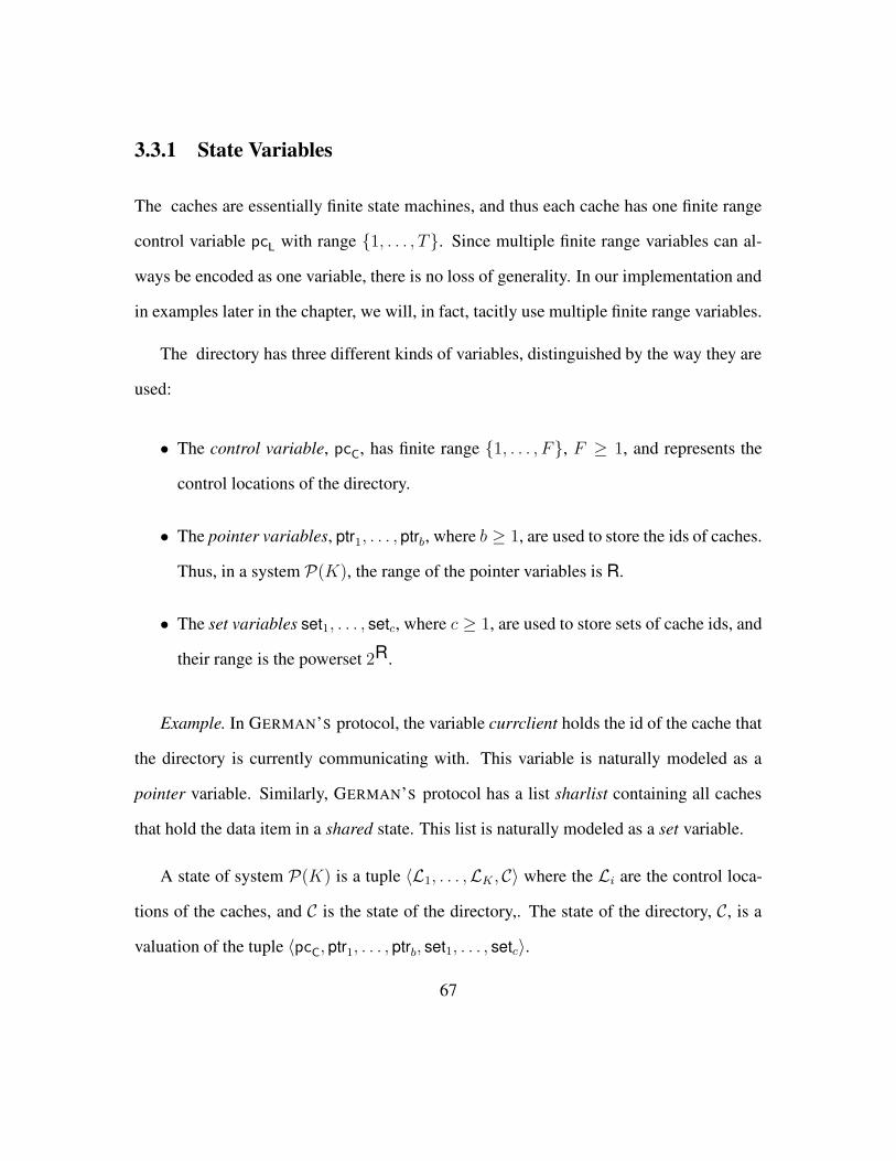
3.3.1 State Variables

The caches are essentially finite state machines, and thus each cache has one finite range

control variable pcL with range 1, . . . , T. Since multiple finite range variables can al-

ways be encoded as one variable, there is no loss of generality. In our implementation and

in examples later in the chapter, we will, in fact, tacitly use multiple finite range variables.

The directory has three different kinds of variables, distinguished by the way they are

used:

• The control variable, pcC, has finite range 1, . . . , F, F ≥ 1, and represents the

control locations of the directory.

• The pointer variables, ptr1, . . . , ptrb, where b ≥ 1, are used to store the ids of caches.

Thus, in a system P(K), the range of the pointer variables is R.

• The set variables set1, . . . , setc, where c ≥ 1, are used to store sets of cache ids, and

their range is the powerset 2R.

Example. In GERMAN’S protocol, the variable currclient holds the id of the cache that

the directory is currently communicating with. This variable is naturally modeled as a

pointer variable. Similarly, GERMAN’S protocol has a list sharlist containing all caches

that hold the data item in a shared state. This list is naturally modeled as a set variable.

A state of system P(K) is a tuple 〈L1, . . . ,LK, C〉 where the Li are the control loca-

tions of the caches, and C is the state of the directory,. The state of the directory, C, is a

valuation of the tuple 〈pcC, ptr1, . . . , ptrb, set1, . . . , setc〉.

67

We shall see below that the ptr variables are used solely to access the state of the

caches. That is, no arithmetic or comparison on ptr variables is allowed. Similarly, set

variables are used either to access caches or in membership queries (i.e., whether a cache

belongs to the set or not). We assume that all variables are used in a type-safe way, that is,

they are assigned or compared only against values from their ranges.

The initial state of the directory and the caches is given by a fixed valuation of all

variables.

3.3.2 Program Description for the Caches

We will describe the transitions of the caches and the central process using a few high level

constructs. Caches have very simple control flow structures, as they can move only from

one control location to another. We can describe the cache transitions using the following

transitions:

pcL = LL1 : goto pcL = LL

2

The semantics of the transition is simple: a cache P (i) in control location LL1 can, at a

nondeterministically chosen timepoint, change its state variable to LL2. The goto statement

is deterministic in the sense that for each location LL1, there is at most one jump goal LL

2.

Note that the state of a cache can also be changed by the directory, see Section 3.3.3.

68

3.3.3 Program Description for the Directory

The directory can execute more complex programs than the cache. In particular, it can

execute a

• simple action to change its control variables, or

• update action to update its pointer or set variables, or

• remote action to change the state of a cache referenced by a pointer.

These basic actions reflect the operations used in a typical directory based cache co-

herence protocol. We will see that, of the above actions, the update action and the remote

action depend on the state of the caches. However, only the remote action can change the

state of a cache. Below we will define the actions in more detail.

A directory transition statement has the form

guard : do actions A1, A2, .., Ak

where A1, . . . , Ak are basic actions as described below, and guard is a condition of the

form pcC = L ∧ Φ(ptr, set). Here, L is a directory control location and Φ(ptr, set) is a

Boolean combination of expressions of the form pcL[ptri] = LL, ptr ∈ seti, or seti = ∅.

The semantics of this statement is as follows:

1. If guard is true, then execute the actions A1, . . . , Ak.

2. The whole transition, including the evaluation of the guard, is executed atomically

in one time step with actions A1, . . . , Ak being executed in that order.

69

3. We will assume that the basic actions in a transition do not conflict with each other.

In other words, no variable should be modified by more that one action. This implies

that there is only one simple action per transition, that no ptr variable is updated by

more than one action, that only one set variable is updated, and that remote actions

are executed on different caches.

We will now describe the basic actions in more detail.

Simple Actions have the format goto pcC = LC, where LC is a directory control location.

The semantics of this action is that the directory control variable pcC is set to LC.

Update Actions come in several formats:

assign ptri = ptrj and assign seti = setj. The next value of ptri is set to the current

value of ptrj .

add ptri to setj and remove ptri from setj. Add or remove the cache pointed to by

ptri from set setj .

pick ptri from SL, where SL is a list of (constant) cache control locations. The

semantics of this action is that the variable ptri is nondeterministically made to point

to one of the caches whose control location is in S L. If there is no such cache, then

ptri is unchanged.

Remote Actions have the form remote V : goto pcL = LL, where LL is a cache control

location and V is a pointer variable. This action enforces the new control location L on

70

the cache pointed to by V . In general, the remote action can also have the form

remote V : map

where map is a switch statement of the form:

switch pcL

LL1 : goto pcL = LL′

1


2

. . .

. . .

This action enforces the cache pointed to by V to execute the switch statement. The remote

action is analogously defined for set variables. A remote action for a set variables forces

all the caches in the set variable to execute the switch statement simultaneously. While

GERMAN’S protocol does not require remote actions on set variables, FLASH protocol

does.

The remote action is used to model the communication from central process to the

local caches. For example, in GERMAN’S protocol, the central directory process sends

invalidate message to all the caches present in the invlist set variable one cache at a time.

The central process first picks a cache present in invlist by assigning a pointer variable

71

temptr1 appropriately. Then the central process writes an invalid message to the incom-

ing channel, chan2, of the cache pointed to by temptr1. Since, we model communication

channels as internal variables of the caches, the effect of central process writing to chan2

can be accurately modelled as a remote action with the general switch statement.

3.3.4 Describing Real-Life Protocols

GERMAN’S protocol and the FLASH protocol can be naturally expressed in our protocol

description language. These protocols share a common basic functionality: when a cache

requests shared access to a data item, the directory grants the request if the data item is

not held in exclusive state by any other cache. Otherwise, the directory sends a message

to the cache having exclusive access to the data item to relinquish control over the data

item. Subsequently, the directory grants shared access to the cache that issued the re-

quest. When a cache requests exclusive access to the data item, the directory grants the

request if no other cache has any form of access to the data item. Otherwise, the direc-

tory sends messages to all caches having access to the data item to invalidate their local

copies. The directory can either wait to receive acknowledgements from the caches (lazy

operating mode) or grant exclusive access to the cache which issued the request (eager

operating mode). In this thesis, we consider the FLASH protocol operating in eager mode

and GERMAN’S protocol operating in lazy mode.

While the basic functionality of many cache coherence protocols essentially follows

the above description, there are a lot of additional low level details that add to the com-

plexity of a directory based protocol and need to be accounted for in our input language.

72

In a typical protocol, the caches communicate with the directory process using dedi-

cated communication channels. The caches execute relatively independently of each other.

Thus, the simple goto statements for caches suffice to model the transitions of the caches.

The directory process usually maintains pointers to caches and also sets of caches. The

pointer and set variables are used to receive and send messages to specific recipients.

Following other work in this area [29; 64], we assume that the communication chan-

nels between caches and the directory are of length 1. The communication channels are

modeled using local variables of the caches. Since the directory can read and write to

the local variables via the remote action, the local variables can simulate communication

channels. For instance, in GERMAN’s protocol we have a central transition statement:

currcmd = empty ∧ read = yes ∧ chan1[currclient] = reqshar:

do actions goto read = no ∧ currcmd = reqshar,

remote currclient: goto chan1 = empty

which shows how the directory communicates with a cache. Here, the pointer variable

currclient points to a local process, and chan1[currclient] is the variable that serves as a

communication channel from the cache to the directory. Note also that there is more than

one control variable in the directory, namely, read, and currcmd.

The above transition says that if there is a reqshar message in channel chan1, the

directory process reads it by updating the variable currcmd using the goto action. After

reading it, the directory removes the message from chan1 using the remote action which

sets chan1 to empty. Broadcast actions can also be described succinctly using remote

actions.

Note that in our language, the protocol is described at a high level without getting

73

into implementation details, reflecting the abstraction level at which designers think about

protocols. This approach is consistent with the current trend towards synthesis of low level

designs from reliable and easily verifiable high level designs.

The full descriptions of the FLASH protocol and GERMAN’S protocol are given in

Section 3.9.

3.4 Environment Abstraction for Cache Coherence Pro-

tocols

In this section, we instantiate environment abstraction for verifying cache coherence pro-

tocols.

3.4.1 Specifications and Labels

Most properties of interest in parameterized systems refer to the control locations: for

example, typical safety properties say that no two caches can hold the same data item in

exclusive state at the same time. Usually we are interested in verifying such properties for

each cache in the system, not for a specific cache. In this chapter, we will consider the

two-indexed safety property

∀x, y.x 6= y ∧ pc[x] = crit⇒ ¬(pc[y] = crit)

This can be equivalently written as a single index property

∀x.(pc[x] = crit⇒ ¬(crit ∈ env(x)))

74

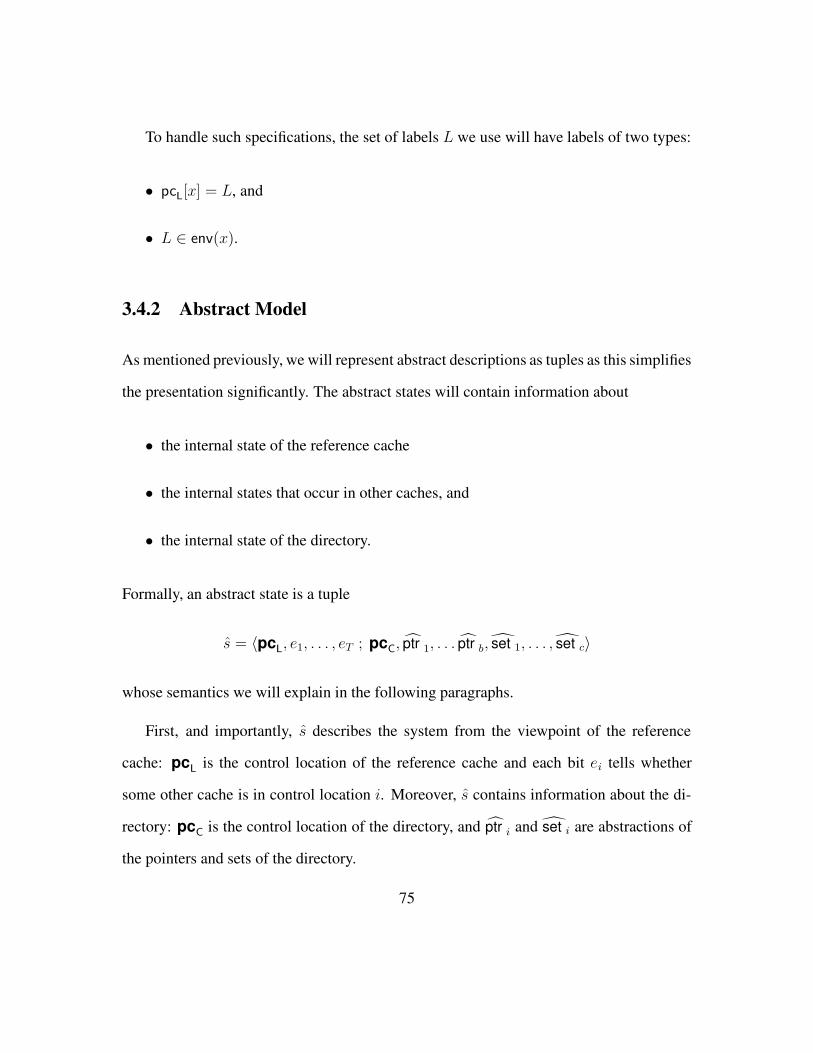
To handle such specifications, the set of labels L we use will have labels of two types:

• pcL[x] = L, and

• L ∈ env(x).

3.4.2 Abstract Model

As mentioned previously, we will represent abstract descriptions as tuples as this simplifies

the presentation significantly. The abstract states will contain information about

• the internal state of the reference cache

• the internal states that occur in other caches, and

• the internal state of the directory.

Formally, an abstract state is a tuple

s = 〈pcL, e1, . . . , eT ; pc

C, ptr 1, . . . ptr b, set 1, . . . , set c〉

whose semantics we will explain in the following paragraphs.

First, and importantly, s describes the system from the viewpoint of the reference

cache: pcL

is the control location of the reference cache and each bit ei tells whether

some other cache is in control location i. Moreover, s contains information about the di-

rectory: pcC

is the control location of the directory, and ptr i and set i are abstractions of

the pointers and sets of the directory.

75

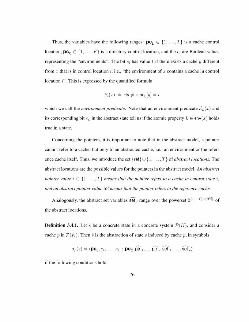
Thus, the variables have the following ranges: pcL∈ 1, . . . , T is a cache control

location, pcC∈ 1, . . . , F is a directory control location, and the ei are Boolean values

representing the “environments”. The bit ei has value 1 if there exists a cache y different

from x that is in control location i, i.e., “the environment of x contains a cache in control

location i”. This is expressed by the quantified formula

Ei(x).= ∃y 6= x.pcL[y] = i

which we call the environment predicate. Note that an environment predicate EL(x) and

its corresponding bit eL in the abstract state tell us if the atomic property L ∈ env(x) holds

true in a state.

Concerning the pointers, it is important to note that in the abstract model, a pointer

cannot refer to a cache, but only to an abstracted cache, i.e., an environment or the refer-

ence cache itself. Thus, we introduce the set ref∪1, . . . , T of abstract locations. The

abstract locations are the possible values for the pointers in the abstract model. An abstract

pointer value i ∈ 1, . . . , T means that the pointer refers to a cache in control state i,

and an abstract pointer value ref means that the pointer refers to the reference cache.

Analogously, the abstract set variables set i range over the powerset 21,...,T∪ref of

the abstract locations.

Definition 3.4.1. Let s be a concrete state in a concrete system P(K), and consider a

cache p in P(K). Then s is the abstraction of state s induced by cache p, in symbols

αp(s) = 〈pcL, e1, . . . , eT ; pc

C, ptr 1, . . . ptr b, set 1, . . . , set c〉

if the following conditions hold:

76

1. In state s, cache p is in control location pcL, i.e.,

s |= pcL

= pcL[p].

“The reference cache is in control location pcL.”

2. Each ei is the truth value of the environment predicate Ei(x) for cache p, i.e.,

s |= ∃y 6= p.pcL[y] = i iff ei = 1.

“The environment contains a cache in control location i. ”

3. The directory is in control location pcC

, i.e.,

s |= pcC = pcC.

“The directory is in control location pcC.”

4. Each pointer ptr i has value abs(ptri), where abs(ptri) is the abstract location pointed

to by ptri, i.e.,

abs(ptri).=

ref if s |= ptri = p

pcL[ptri] otherwise

.

“The i-th pointer points to the abstract location ptr i.”

5. The sets set i generalize the pointers in the natural way, i.e.,

set i.= abs(q) : q ∈ seti.

“The i-th set variable points to the set set i of abstract locations.”

77

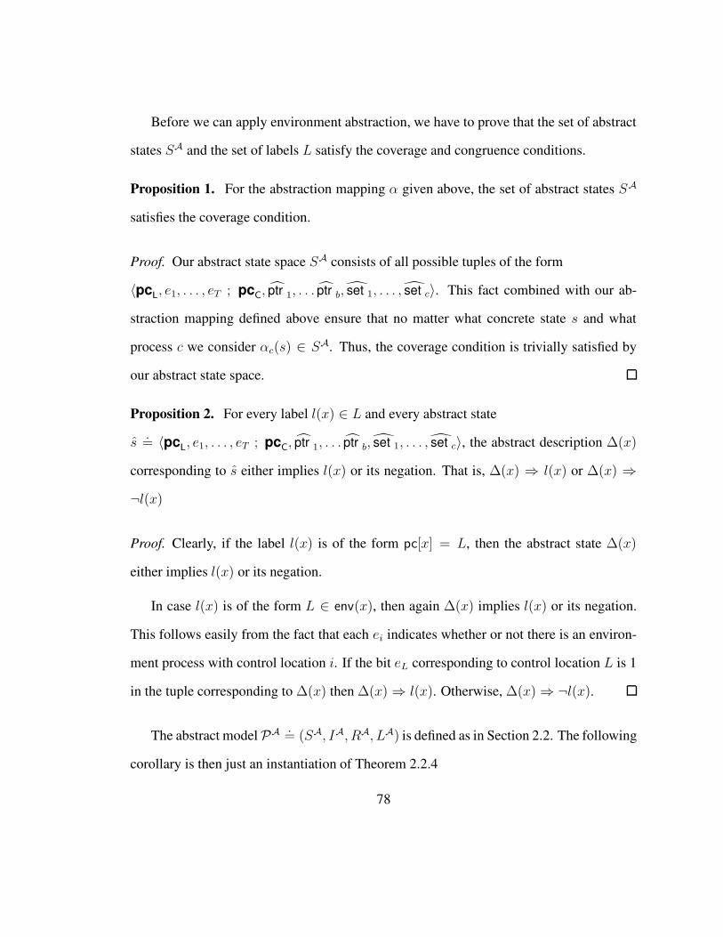
Before we can apply environment abstraction, we have to prove that the set of abstract

states SA and the set of labels L satisfy the coverage and congruence conditions.

Proposition 1. For the abstraction mapping α given above, the set of abstract states SA

satisfies the coverage condition.

Proof. Our abstract state space SA consists of all possible tuples of the form

〈pcL, e1, . . . , eT ; pc

C, ptr 1, . . . ptr b, set 1, . . . , set c〉. This fact combined with our ab-

straction mapping defined above ensure that no matter what concrete state s and what

process c we consider αc(s) ∈ SA. Thus, the coverage condition is trivially satisfied by

our abstract state space.

Proposition 2. For every label l(x) ∈ L and every abstract state

s.= 〈pc

L, e1, . . . , eT ; pc

C, ptr 1, . . . ptr b, set 1, . . . , set c〉, the abstract description ∆(x)

corresponding to s either implies l(x) or its negation. That is, ∆(x) ⇒ l(x) or ∆(x) ⇒

¬l(x)

Proof. Clearly, if the label l(x) is of the form pc[x] = L, then the abstract state ∆(x)

either implies l(x) or its negation.

In case l(x) is of the form L ∈ env(x), then again ∆(x) implies l(x) or its negation.

This follows easily from the fact that each ei indicates whether or not there is an environ-

ment process with control location i. If the bit eL corresponding to control location L is 1

in the tuple corresponding to ∆(x) then ∆(x)⇒ l(x). Otherwise, ∆(x)⇒ ¬l(x).

The abstract modelPA .= (SA, IA, RA, LA) is defined as in Section 2.2. The following

corollary is then just an instantiation of Theorem 2.2.4

78

Corollary 2 (Soundness of Abstraction). Let P(N) be a parameterized cache coherence

system and PA. Consider a control specification ∀x.φ(x). If PA |= φ(x) then P(N) |=

∀x.φ(x).

From Environment Bits to Counters

To keep the presentation simple we have represented the variables ei as bits which

indicate whether there exists a cache in control location i. To make the abstraction more

precise, the ei can be easily generalized to counters of range, e.g., 0, 1, 2, where 2 is

called the counter threshold. Then ei = 0 means that there is no cache y 6= x in control

location i, ei = 1 means that there is exactly one cache y 6= x in control location i, and

ei = 2 means that at least two caches y 6= x are in control location i. All results in

this chapter can be readily generalized to counter thresholds, and our tool also supports

arbitrary counter thresholds.

3.5 Optimizations to Reduce the Abstract State Space

79

3.5.1 Eliminating Unreachable Environments

The abstract model as described so far has a environment bit eL for each possible local state

L of the caches. It may be the case that not all possible local states are indeed reachable and

the corresponding abstract bits (or counters), which are redundant, can be eliminated. Our

experiments in fact indicate that this kind of optimization achieves significant reduction in

the size of the abstract model.

Finding the local reachable states can be done as follows. First note that the local

state of a cache can change in two ways: 1) the cache executes a local goto action, or 2)

the central process changes the state of the cache using a remote action. Considering the

former case, if a local state s1 is reachable and there is a local transition

pcL = s1 : goto pcL = s2

then local state s2 is reachable as well. Thus, we add a transition (s1, s2) to a reachability

relation R (the reachability relation R is initially empty).

For the latter case, consider a remote action:

remote V : map

where map is a switch statement of the form

80

switch pcL


1


2

. . .

. . .

Here V can be a pointer variable or a set variable. In case V is a pointer variable, we

will say V can point to a local state s if a cache in state s can be pointed to by V . Similarly,

if V is a set variable, we will say V can point to a local state s if a cache in state s can

belong to the set V .

Now, if V can point to local state s1 = LL1 and s1 is a reachable local state then the

local state s2 = LL′

1 is also reachable. Thus, we add (s1, s2) to R as well. By syntactically

examining the protocol code, we can determine an over-approximation of all the local

states that V can point to, as described below.

First consider the case where V is a pointer variable. Suppose V is the pointer variable

ptri and the central process assigns V a value using an action of the form

pick ptri from SL.

The pointer V = ptri can point to any location in SL. Finding the union of SL’s from

all actions that modify V gives us an over-approximation of the set of all caches locations

81

that V can point to. Call this set of locations S. For every, s ∈ S we add (s, s′), where s′

is the location that s is mapped to by map, to the reachability relation R.

In case V is a set variable the over-approximation of the set of location V can point to

is computed as in Remark 8.

Once we have R, an over-approximation to the set of reachable local states is given

by R∗(init) where init is the initial state of the caches. It is enough to have counters

corresponding to only these reachable locations.

3.5.2 Redundancy of the Abstract Set Variables

In this section we will describe how the set variables can be eliminated from many real

protocols including GERMAN’S protocol and the FLASH protocol by a straightforward

program analysis. In the following sections, we can therefore assume that no set variables

are present. The evident motivation to eliminate the set variables is state explosion. Since

each concrete set variable gives rise to an abstract set variable with domain 21,...,T,ref, the

abstract model may become prohibitively large.

Our method is based on the observation that in many real-life protocols, the following

pattern occurs: whenever a cache is added to a set by an add action, then the same tran-

sition also contains a remote action which determines the control location of the cache

(that is, when an add ptri to setj action occurs a remote ptri ... action occurs as well). In

practice, this means that whenever a cache is added to a list, it also receives a message.

Similarly, each remove action is also accompanied by a remote action. Set variables fol-

lowing this pattern are in fact often redundant, that is, conditions involving sets can be

82

replaced by equivalent conditions on the local states of the caches. We will now describe

how to determine if a set is redundant.

Let us fix a set variable setj. Then we can partition the statements in the program D

of the directory into three sets:

• T inj is the set of remote actions which occur together with an action of the form

add ptri to setj.

• T outj is the set of remote actions which occur together with an action of the form

remove ptri from setj .

• The remaining remote actions in the program are collected in the set T restj .

Using these three sets T inj , T outj and T restj , we will compute three sets of cache states

Rinj , Rout

j , Rrestj . Intuitively, Rin

j will be the set of all states that a cache can have while

it is a member of setj. Similarly, Routj contains all states that occur in caches that are not

members of setj .

Given a set of cache states S, the set r(S) is the set of all states reachable from states

in S by local transitions (i.e., goto’s in the program of the cache) and by remote actions in

T restj . Note that for a given set S, r(S) can be obtained by a simple syntactic computation

on the program. With this notation, we can easily describe Rinj , R

outj , and Rrest

j .

• Rrestj is the set of cache states reachable from the initial cache states, i.e., Rrest

j =

r(Iinit).

83

• Rinj is computed as follows: We collect all jump goals of remote 1 actions in T inj

into a set Iin. Then Rinj is the set of cache states reachable from Iin, i.e., r(Iin).

• Routj is computed analogously toRin

j , with Iin replaced by Iout, the set of jump goals

in T outj .

If the sets Rrestj , and Rout

j do not share any common elements with Rinj , then the vari-

able setj is redundant in the sense of the following theorem:

Theorem 3.5.1. Assume that Rrestj ∩ Rin

j = ∅ and Routj ∩R

inj = ∅, and consider a global

state s of a concrete system P(K) with a process p. Then

s |= p ∈ setj iff s |= pcL[p] ∈ Rinj ,

i.e., process p is contained in setj iff its control location is in Rinj .

Proof. Consider first the sets Rrestj and Rin

j . Since Rrestj ∩Rin

j = ∅ (that is, these two sets

are mutually exclusive), a process can have state from Rinj only if some central transition

(of the directory) adds it to the variable setj . Recall that we assumed that a process is put

on a list simultaneously with being sent a message.

Further, since Rinj and Rout

j are mutually exclusive, i.e., Routj ∩R

inj = ∅, a process with

a state in Rinj must belong to the set variable setj. Thus, a process belongs to setj if and

only if its state is in Rinj .

1Jump goals of a remote action are simply the control locations appearing after the goto’s in the remote

action.

84

Remark 8. Note that, for the optimization presented in the previous section, an over-

approximation to the local states that setj can point to is given by Rinj .

In the following sections we will assume that all the set variables appearing in a proto-

col are redundant according to the criterion presented in this section.

3.6 Computing the Abstract Model

In this section we describe how to extract an overapproximation of the abstract model

PA from the program text. The main challenge arises from the fact that there are infinite

number of concrete systems to consider. To solve this problem, we consider each transition

statement of the program separately and over-approximate the set of abstract transitions it

can lead to. This over-approximation can be expressed by an invariant on the current state

and next state variables. The disjunction of all these invariants is the abstract transition

relation. To keep the presentation simple, we will assume that set variables have been

removed using the redundancy criteria presented previously.

The abstract transition relation RA is computed as a series of transition invariants be-

tween current abstract state s and the next abstract state s′. We consider each transition

statement t appearing in the protocol code and find out what abstract transitions it can

lead out. The set of abstract transitions corresponding to a concrete transition statement is

described by a transition invariant I(t). The abstract transition relation RA is then given

by∨

t

I(t)

85

We first consider the case where t is a local transition statement of a cache and later

consider the more complicated case where t is a central transition statement.

3.6.1 Cache Transitions

Recall that caches can only make simple transitions t of the form

pcL = LL1 : goto pcL = LL

2.

This transition can be made either (i) by the reference cache or (ii) by one of the environ-

ment caches.

We will now give conditions when to include an abstract transition from

s = 〈pcL, e1, . . . , eT ,pc

C, ptr 1, . . . , ptr b〉 to

s′ = 〈pc′L, e′1, . . . , e

′T ,pc′

C, ptr

′

1, . . . , ptr′

b〉 corresponding to the transition statement t.

Case (i): Transition by reference cache. The local transition t is executed by the

reference case. In this case, we require that

pcL = LL1 ∧ pcL

′ = LL2 (3.1)

and all other variables are the same in s and s′. Note that no abstract pointers of the

directory need to be changed because the abstract pointers have a special value ref for the

reference cache.

Case (ii): Transition by cache in environment. The local transition t is executed by an

environment cache. In this case, we have the obvious condition that there is a cache in

86

state LL1 before the transition, and also a cache in LL

2 after the transition:

eLL1

= 1 ∧ e′LL

2= 1. (3.2)

Moreover, we have to make sure that the pointers of the directory are changed in accor-

dance with the transition. Let if φ then α else β denote the formula (φ ∧ α) ∨ (¬φ ∧ β).

Then, looping over all pointer variables ptr1 to ptrb, we include the condition below, which

we denote by Λ(L1, L2)

∧

1≤i≤b

if ptr i 6= LL1 then ptr i = ptr

′

i else

if e′LL

1= 0 then ptr

′

i = LL2 else ptr

′

i ∈ LL1, L

L2 .

Intuitively, Λ(LL1, L

L2) expresses the following: if the pointer does not point at LL

1, then

it remains unchanged. Otherwise, one of two things can happen after the transition. First,

if there is no cache left in location LL1 i.e., e′

LL1

= 0, then the cache referred to by the pointer

must have moved, and thus, the pointer has to be updated to point to LL2. Second, if a cache

is left in location LL1, then it is not clear which cache moved, and we over-approximate.

Again, all other variables are the same in s and s′.

The abstract invariant I(t) corresponding to the transition statement t is given by the

disjunction of 3.1 and 3.2.

Lemma 3.6.1. Let s, s′ be two states of a concrete system P(K). Let there be a transition

from s to s′ with process c executing a local transition. Then the abstract states αc(s) and

αc(s′) satisfy the invariant described by I(t).

Proof. The proof of this lemma follows simply from the way we constructed I(t).

87

3.6.2 Directory Transitions

Consider now the case where the transition statement t is a directory transition. Recall

that the directory transitions have the form

pcC = L ∧ Φ(ptr, set) : do actions A1, .., Ak.

Each directory transition t will be translated into a condition

pcC

= L ∧ Φ ∧ IA1 ∧ . . .IAk ∧R

where the IAi are the abstract conditions corresponding to the actionsAi, andR constrains

all the abstract variables not appearing elsewhere to be the same in s and s′.

We will first show how to translate each basic action Ai into a condition IAi .

• For the simple action goto LC we obtain the natural condition pc′C

= LC.

• For the update action assign ptr1 = ptr2 we obtain the condition ptr′

1 = ptr 2.

• For the update action pick ptr from S L we obtain the condition

(pcL∈ SL ∧ ptr

′= ref) ∨ (ej = 1 ∧ j ∈ SL ∧ ptr

′= j)

∨(pcL6∈ SL ∧

∧j∈SL ej = 0 ∧ ptr

′= ptr ).

Intuitively, if the reference process has a control location from the set S L then, in

the new state, ptr can point to the reference process. Thus, we have the disjunct

pcL∈ SL ∧ ptr

′= ref. Alternatively, some environment process might have a

88

control location from the set SL and the pointer variable can point to it in the next

state. Thus, we have the disjunct ej = 1 ∧ j ∈ SL ∧ ptr′= j. Lastly, it is possible

that none of the caches have control locations from the set S L. In this case, the

value of the pointer variable does not change. Hence we have the disjunct pcL6∈

SL ∧∧j∈SL ej = 0 ∧ ptr

′= ptr .

• For the remote action remote ptr : goto pcL = LL we obtain the condition

(ptr = ref ∧ pc′L

= LL) (3.3)∨

∨

1≤L≤T

(ptr = L ∧ ptr′= LL ∧ e′LL = 1 ∧ Λptr(L, L

L)) (3.4)

where Λptr(L, LL) is defined as

∧

1≤i≤b, ptri6=ptr

if ptr i 6= L then ptr i = ptr′

i else

if e′L = 0 then ptr′

i = LL else ptr′

i ∈ L, LL .

Note that Λptr(L, LL) is similar to Λ(L, LL) defined in Section 3.6.1 except that

pointer ptr is left unchaned.

The explanation for this abstract transition is quite simple. If the pointer ptr, which is

used in the remote action, points to the reference process, then the control location

of the reference process is changed to LL. Thus, we have the disjunct (ptr = ref ∧

pc′L

= LL) shown in Equation 3.3.

To understand the second disjunct, shown in Equation 3.4, consider the case where

ptr points to an environment process. Suppose the environment process is in envi-

ronment eL, that is, ptr = L. Then the following hold:

89

– In the next state, the pointer variable points to a process in environment eLL

because the new state of the cache pointed to by ptr is LL. Thus, we have the

condition ptr′= LL

– In the next state, the environment eLL is non-empty, that is, e′LL = 1. The

environment eL could be 0 or 1 in the next state.

– Since a process moves from environment eL to eLL pointer variables other than

ptr must be updated according to the condition Λptr(L, LL)

Putting all the above together, we have the condition

(ptr = L ∧ ptr′= LL ∧ e′LL = 1 ∧ Λptr(L, L

L)).

The case where the remote action is of the more general form with map involving

set variables is similar to the case described above.

Remark 9. Since the set variables are redundant, add and remove actions are irrelevant

for the construction of the abstract model.

Assuming that the set variables are redundant in the sense of Section 3.5, the abstrac-

tion Φ of the condition Φ(set, ptr) is obtained by abstracting each atomic subformula:

• pcL[ptri] = LL is abstracted into (ptr i = ref ∧ pcL

= LL) ∨ ptr i = LL.

• ptri ∈ setj is abstracted into (ptr i = ref ∧ pcL∈ Rin

j ) ∨ (ptr i 6= ref ∧ ptr i ∈ Rinj ).

• setj = ∅ is abstracted into pcL/∈ Rin

j ∧∧s∈Rin

jes = 0. In other words, no cache

should be in a state from Rinj ; hence pc

L/∈ Rin

j , and all counters corresponding to

states in Rinj must be 0.

90

Lemma 3.6.2. Let s, s′ be two states of a concrete system P(K). Let there be a transition

from s to s′ with the directory process executing the statement t. Then the abstract states

αc(s) and αc(s′) for any process c ∈ [1..K] together satisfy the transition invariant I(t).

Proof. The proof of this lemma follows simply from the way we constructed I(t).

3.7 Experiments

GERMAN’S cache coherence protocol [44; 66] and FLASH cache coherence protocol [63]

are the two most widely studied cache coherence protocols. We applied our abstraction

technique to several versions, including the standard, correct version, of the GERMAN’S

protocol and a simplified version of the FLASH protocol.

GERMAN’s protocol, which operates in lazy mode, has two set variables sharlist and

invlist. Whenever a cache enters a shared state it is added to sharlist. The variable sharlist

is redundant according to the criterion in Section 3.5. The variable invlist is used to send

invalidate messages to caches which are in a shared state. Initially, invlist is set equal to

sharlist. When an invalidate message is sent to a cache in invlist, it is removed from invlist.

While invlist is not redundant according to the criterion of Section 3.5, a simple change

makes our criterion applicable: instead of initializing invlist by assigning sharlist to it, we

can add a cache to invlist whenever it is added to sharlist. This simple change makes the

set variable invlist redundant, too. All the different versions of the GERMAN’S protocol

that we verified had this modification 2.2Alternatively, we can also create a stronger redundancy criterion for set variables, which will ensure

that invlist is redundant without any modification. But, the modification we introduced is minor and does

91

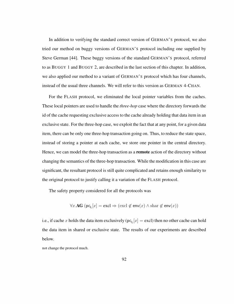
In addition to verifying the standard correct version of GERMAN’S protocol, we also

tried our method on buggy versions of GERMAN’S protocol including one supplied by

Steve German [44]. These buggy versions of the standard GERMAN’S protocol, referred

to as BUGGY 1 and BUGGY 2, are described in the last section of this chapter. In addition,

we also applied our method to a variant of GERMAN’S protocol which has four channels,

instead of the usual three channels. We will refer to this version as GERMAN 4-CHAN.

For the FLASH protocol, we eliminated the local pointer variables from the caches.

These local pointers are used to handle the three-hop case where the directory forwards the

id of the cache requesting exclusive access to the cache already holding that data item in an

exclusive state. For the three-hop case, we exploit the fact that at any point, for a given data

item, there can be only one three-hop transaction going on. Thus, to reduce the state space,

instead of storing a pointer at each cache, we store one pointer in the central directory.

Hence, we can model the three-hop transaction as a remote action of the directory without

changing the semantics of the three-hop transaction. While the modification in this case are

significant, the resultant protocol is still quite complicated and retains enough similarity to

the original protocol to justify calling it a variation of the FLASH protocol.

The safety property considered for all the protocols was

∀x.AG (pcL[x] = excl⇒ (excl 6∈ env(x) ∧ shar 6∈ env(x))

i.e., if cache x holds the data item exclusively (pcL[x] = excl) then no other cache can hold

the data item in shared or exclusive state. The results of our experiments are described

below.

not change the protocol much.

92

Standard German’s protocol. We first applied our method to the standard, correct

version of GERMAN’s protocol. We did not use the optimization to eliminate the counters

for unreachable local states. For this unoptimized version, Cadence SMV took about 3

hours (11400 seconds) to verify the safety property. We then applied the optimization

to eliminate the counters corresponding to unreachable local states. Instead of writing a

procedure to find the unreachable states, we supplied a list of unreachable local states to

the abstraction program manually as it is easy to figure out manually what local states are

unreachable. For instance, for GERMAN’S protocol, it is easy to see that if the outgoing

channel chan3 is carrying an invack message then the cache state must be invalid. While

the list of states we supplied may be not exhaustive, it still gives significant reduction in the

abstract state space. With this optimization, SMV takes about 5 minutes to complete the

verification. This running time compares favorably with other verification efforts involving

GERMAN’S protocol, see for instance [3].

Version Buggy 1. In the BUGGY 1 version, after the directory grants exclusive access

to a cache, it fails to set the grantexcl variable to true. Thus, when another cache requests

shared access, it gets the access even though the first cache holds it in exclusive state. We

applied our abstraction (without the optimization to eliminate counters corresponding to

unreachable states) and applied Cadence SMV’s Bounded Model Checker. BMC takes

around 15 mins to find the bug at depth 12 (that is, the bug is reached after 12 transitions

have been executed by the cache coherence system).

Version Buggy 2. In the BUGGY 2 version, the directory grants a shared request even

if grantexcl variable is true. As with the previous version, we constructed the abstract

model without using the optimization to remove counters for unreachable states. BMC

93

again takes under 15 mins to find the bug at depth 12.

German 4-Chan. In this variant of GERMAN’S protocol, there are four channels

instead of the usual three channels. In specific, instead of just one incoming channel, there

are two incoming channels, chan2 and chan4, for every cache. In the original version,

the single incoming channel carries all three types of messages: grantshar, grantexcl

and invalid. In the four channel version, one of the incoming channels, chan2 carries

grantshar and grantexcl messages while the other one, chan4, carries invalid message.

Having two incoming channels leads to the following subtle bug: cache 1 requests a shared

access, and while this is being processed, it sends out another request. The first request is

honored and cache 1 gets shared access (while the other request for shared access is still

pending). Now the central process reads the second request from cache 1, and sends it

another grantshar message on chan2.

Immediately after this, another cache, say cache 2, requests exclusive access. Before

granting exclusive access to cache 2, the central process sends out an invalidate message to

all caches with shared access, including cache 1 on the second incoming channel chan4.

Cache 1 reads the invalid message on chan4 (while chan2 still has the grantshar mes-

sage) and transitions to invalid state and sends an acknowledgement to the central process

(on chan3). Once the central process sees all the acknowledgements, it grants exclusive

access to cache 2. But, the grantshar message is still present in chan2 of cache 1 and this

leads cache 1 to transition to a shared state. Thus, cache 1 ends with shared access while

cache 2 still has exclusive access.

We applied our abstraction method (with both the optimizations described in Sec-

94

tion 3.5) and used a BDD based model checker to find the bug. It took SMV 7 mins

to find the bug at depth 15. BMC runs out of memory at depth 15. Note that BMC takes

less than 15 mins for the two buggy versions because the counter example depth is only

12. For these buggy versions, BDD based model checker does not finish even after an hour

(the abstract models for buggy versions were not optimized).

Flash protocol. We constructed an abstract model for FLASH protocol using both the

optimizations described in Section 3.5. With counter threshold 1 (cf. Section 3.4.2), we

get a spurious counterexample due to the three-hop case. The spurious counter example is

as follows: suppose counter eexcl corresponds to an exclusive local state. Suppose now that

the reference process requests exclusive access. The central process forwards this request

to the environment process which is represented by the counter eexcl. After serving the

request the environment process goes into an invalid state, and thus eexcl should become 0.

But, since 1 stands for many in the abstract model, there is an abstract transtion that keeps

eexcl as 1. This leads to the violation of the safety property.

To get rid of this spurious counterexample, we track counters corresponding to exclu-

sive local states more carefully. We refine the abstract model by increasing the counter

threshold to 2 for those environments where the cache is in the exclusive state. The result-

ing model is precise enough to prove the safety property. The model checking time was

about 7 hours (25700 seconds).

The table shown in Figure 3.1 summarizes our experimental results.

Remark 10. For the protocols that do not satisfy the cache coherence property, the coun-

terexamples always involve just two caches. For example, the version of GERMAN’S

95

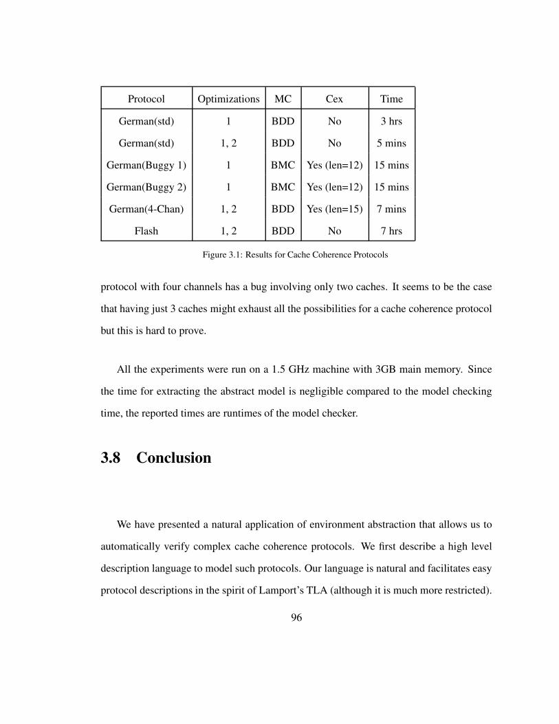
Protocol Optimizations MC Cex Time

German(std) 1 BDD No 3 hrs

German(std) 1, 2 BDD No 5 mins

German(Buggy 1) 1 BMC Yes (len=12) 15 mins

German(Buggy 2) 1 BMC Yes (len=12) 15 mins

German(4-Chan) 1, 2 BDD Yes (len=15) 7 mins

Flash 1, 2 BDD No 7 hrs

Figure 3.1: Results for Cache Coherence Protocols

protocol with four channels has a bug involving only two caches. It seems to be the case

that having just 3 caches might exhaust all the possibilities for a cache coherence protocol

but this is hard to prove.

All the experiments were run on a 1.5 GHz machine with 3GB main memory. Since

the time for extracting the abstract model is negligible compared to the model checking

time, the reported times are runtimes of the model checker.

3.8 Conclusion

We have presented a natural application of environment abstraction that allows us to

automatically verify complex cache coherence protocols. We first describe a high level

description language to model such protocols. Our language is natural and facilitates easy

protocol descriptions in the spirit of Lamport’s TLA (although it is much more restricted).

96

In contrast to previous approaches [67], we use symbolic model checkers in this chapter.

To keep the computation feasible, we over-approximate the abstract transition system

one statement at a time, similar to predicate abstraction for software. Moreover, we use the

results of Section 3.5 to eliminate semantically redundant set variables, and thus to reduce

the size of the abstract models.

In the next section, we present the descriptions of the protocols that we verified. In

the next chapter we will consider the application of environment abstraction to mutual

exclusion protocols.

3.9 Protocol Descriptions

A simplified version of the FLASH cache coherence protocol is shown in our input lan-

guage below. The simplifications are as follows:

• In the original FLASH protocol, the directory (i.e. the central process) distinguishes

between the home cache and the other caches. While our abstraction method can

handle the full version, the current model checkers cannot handle the abstract model

that is generated.

• The communication between the central process (directory) and local processes (the

caches) is modelled by having two variables chanin and chanout per cache. These

two variables serve as incoming and outgoing channels for each cache. Use of two

variables implies that the communication buffers are bounded, in fact, are of size 1.

This restriction is similar to the restriction seen in GERMAN’s Protocol.

97

• For the three-hop case, we exploit the fact that at any point in time, for a given

cache line, there can be only one three-hop transaction. This fact can be seen just

by examining the code for the central process. So to reduce state space, instead of

storing a pointer at each cache, we store one pointer at the central process (named

threeptr in the model below). Since there is only one three-hop transaction and all

the information on the caches involved is known, we model the three-hop transaction

as part of the central process. This does not change the semantics of the three-

hop transaction in any way, it is just a convenient representation in our modelling

language.

The central process reads a message from a cache via a transition involving pick ac-

tion. For example, the transition

currcmd = empty ∧ read = no: Do Actions

goto currcmd = get ∧ read = yes

pick temptr from chanout = get

says, if current command (CURRCMD) is empty, and nothing has been read (READ =

no), then do the action pick temptr from chanout = get. This action sets the pointer

temptr to some cache satisfying the condition chanout = get, that is, some cache which

has sent a get message. Then the current command is set to get and READ is marked yes.

The expression sharlist = Φ indicates that the set sharlist is empty. Finally, the

statement remote sharlist goto chanin = inv denotes the action where all caches present

in sharlist get an invalidate (inv) message.

98

FLASH PROTOCOL

Local Process

Local Vars

CACHESTATE: inv, shar, excl;

INVMARKED: yes, no;

CHANIN: empty, put, putx, inv, NAK;

CHANOUT: empty, get, getx, invack;

Local Transitions

cachestate = inv ∧ chanout = emtpy: goto chanout = get

cachestate = inv ∧ chanout = emtpy: goto chanout = getx

cachestate = shar ∧ chanout = emtpy: goto chanout = getx

cachestate = inv ∧ chanin = inv: goto invmarked = yes

cachestate = inv ∧ invmarked = no ∧ chanin = put: goto cachestate = shar ∧

chanin = empty

99

cachestate = inv ∧ invmarked = yes ∧ chanin = put: goto invmarked = no ∧

chanin = empty

cachestate = inv ∧ invmarked = no ∧ chanin = putx: goto cachestate = excl ∧

chanin = empty

cachestate = inv ∧ invmarked = yes ∧ chanin = putx: goto invmarked = no ∧

chanin = empty

cachestate = shar ∧ chanin = inv: goto cachestate = inv ∧ chanout = invack

cachestate = excl ∧ chanin = inv: goto cachestate = inv ∧ chanout = invack

cachestate = inv ∧ chanin = NAK: goto chanin = empty

cachestate = shar ∧ chanin = NAK: goto chanin = empty

Central Process

Central vars

DIRTY: no, yes;

PENDING: no, yes;

HDPTR: ptr;

HDVALID: no, yes;

CURRCMD: empty, get, getx, invack;

THREEHOP: empty, get, get1, getx, getx1;

THREEHOPTR: ptr;

CHECKSHRLIST: no, yes;

SHARLIST: set;

TEMPTR: ptr;

100

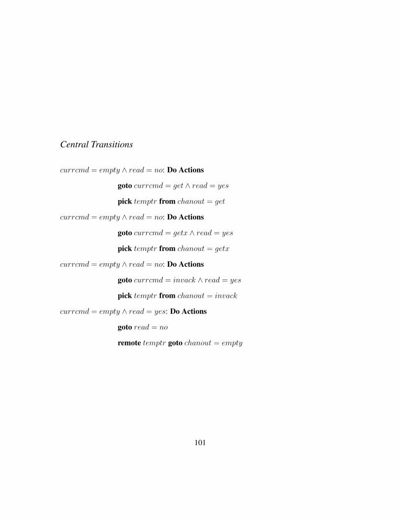
Central Transitions


goto currcmd = get ∧ read = yes

pick temptr from chanout = get


goto currcmd = getx ∧ read = yes

pick temptr from chanout = getx


goto currcmd = invack ∧ read = yes

pick temptr from chanout = invack

currcmd = empty ∧ read = yes: Do Actions

goto read = no

remote temptr goto chanout = empty

101

currcmd = get∧read = no∧pending = no∧dirty = no∧chanout[temptr] = empty:

Do Actions

goto currcmd = empty

remote temptr goto chanin = put

currcmd = get∧read = no∧pending = no∧dirty = yes∧chanout[temptr] = empty:

Do Actions

goto currcmd = empty ∧ threehop = get ∧ pending = yes

assign threehoptr = temptr

threehop = get ∧ cachestate[hdptr] = excl: Do Actions

goto threehop = get1

remote hdptr goto cachestate = inv

currcmd = get∧read = no∧pending = yes∧ chanout[temptr] = empty: Do Actions


remote temptr goto chanin = NAK

currcmd = getx ∧ read = no ∧ pending = yes ∧ chanout[temptr] = empty: Do

Actions


remote temptr goto chanin = NAK

102

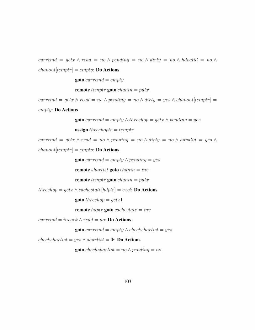
currcmd = getx ∧ read = no ∧ pending = no ∧ dirty = no ∧ hdvalid = no ∧

chanout[temptr] = empty: Do Actions


remote temptr goto chanin = putx

currcmd = getx ∧ read = no ∧ pending = no ∧ dirty = yes ∧ chanout[temptr] =

empty: Do Actions

goto currcmd = empty ∧ threehop = getx ∧ pending = yes

assign threehoptr = temptr

currcmd = getx ∧ read = no ∧ pending = no ∧ dirty = no ∧ hdvalid = yes ∧

chanout[temptr] = empty: Do Actions

goto currcmd = empty ∧ pending = yes

remote sharlist goto chanin = inv

remote temptr goto chanin = putx

threehop = getx ∧ cachestate[hdptr] = excl: Do Actions

goto threehop = getx1

remote hdptr goto cachestate = inv

currcmd = invack ∧ read = no: Do Actions

goto currcmd = empty ∧ checksharlist = yes

checksharlist = yes ∧ sharlist = Φ: Do Actions

goto chechsharlist = no ∧ pending = no

103

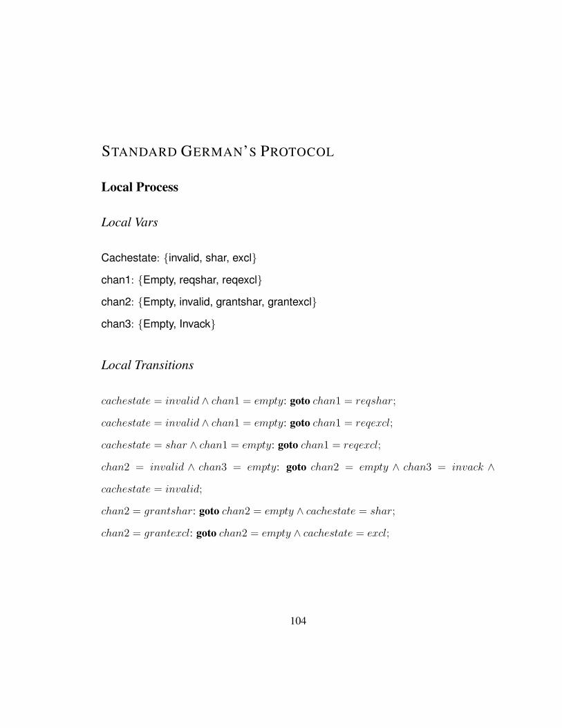
STANDARD GERMAN’S PROTOCOL

Local Process

Local Vars

Cachestate: invalid, shar, excl

chan1: Empty, reqshar, reqexcl

chan2: Empty, invalid, grantshar, grantexcl

chan3: Empty, Invack

Local Transitions

cachestate = invalid ∧ chan1 = empty: goto chan1 = reqshar;

cachestate = invalid ∧ chan1 = empty: goto chan1 = reqexcl;

cachestate = shar ∧ chan1 = empty: goto chan1 = reqexcl;

chan2 = invalid ∧ chan3 = empty: goto chan2 = empty ∧ chan3 = invack ∧

cachestate = invalid;

chan2 = grantshar: goto chan2 = empty ∧ cachestate = shar;

chan2 = grantexcl: goto chan2 = empty ∧ cachestate = excl;

104

Central Process

Central Vars

exclgrant: yes, no

currcmd: empty, reqshar, reqexcl

currclient: ptr

sharlist: set

Invlist: set

read: yes, no

tmpread1: no, yes

temptr2: ptr

tmpread2: no, yes

temptr1: ptr

Central Transitions


goto read = yes

pick currclient from local | chan1[local]=reqshar ∨

chan1[local]=reqexcl

currcmd = empty ∧ read = yes ∧ chan1[currclient] = reqshar: Do Actions

goto read = no ∧ currcmd = reqshar

remote currclient goto chan1 = Empty

105

currcmd = empty ∧ read = yes ∧ chan1[currclient] = reqexcl: Do Actions

goto read = no ∧ currcmd = reqexcl


assign Invlist = sharlist

currcmd = reqshar ∧ grantexcl = no ∧ chan2[currclient] = empty: Do Actions


remote currclient goto chan2 = grantshar

Add currclient to sharlist

currcmd = reqexcl ∧ sharlist = Φ ∧ chan2[currclient] = empty: Do Actions

goto currcmd = empty ∧ grantexcl = yes

remote currclient goto chan2 = grantexcl


currcmd = reqshar ∧ tmpread1 = no ∧ grantexcl = yes: Do Actions

goto tmpread1 = yes

pick temptr1 from local |(local ∈ Invlist)∧ chan2[local ] = Empty

currcmd = reqexcl ∧ tmpread1 = no: Do Actions

goto tmpread1 = yes

pick temptr1 from local |(local ∈ Invlist)∧ chan2[local ] = Empty

currcmd = reqshar ∧ tmpread1 = yes: Do Actions

goto tmpread = no

remote temptr1 goto chan2 = invalid

Remove temptr1 from Invlist

106


goto tmpread1 = yes




goto tmpread2 = yes

pick temptr2 from local |chan3[local ] = invack


goto tmpread1 = yes



goto tmpread2 = no ∧ grantexcl = no

remote temptr2 goto chan3 = Empty

currcmd = reqexcl ∧ tmpread2 = yes: Do Actions



Remove temptr2 from sharlist

107

BUGGY VERSIONS OF GERMAN’S PROTOCOL

As a sanity check, we created two buggy versions of GERMAN’S protocol to see if our

method is able to catch the bugs. The buggy versions are described below.

Buggy version 1. In the first buggy version, after the directory grants exclusive access to a

cache, it fails to set the grantexcl variable to true. That is, instead of the correct transition





we have the faulty version





108

Buggy version 2. For the second buggy version, the directory grants a shared request even

if grantexcl variable is true (that is, some cache has been granted exclusive access). Thus,

instead of the normal transition





we have

currcmd = reqshar ∧ grantexcl = yes ∧ chan2[currclient] = empty: Do Actions




109

GERMAN’S PROTOCOL WITH EXTRA CHANNELS (4-CHAN)

Local Process

Local Vars

Cachestate: invalid, shar, excl

chan1: Empty, reqshar, reqexcl

chan2: Empty, grantshar, grantexcl

chan3: Empty, Invack

chan4: Empty, invalid

Local Transitions

cachestate = invalid ∧ chan1 = empty: goto chan1 = reqshar;

cachestate = invalid ∧ chan1 = empty: goto chan1 = reqexcl;

cachestate = shar ∧ chan1 = empty: goto chan1 = reqexcl;

chan4 = invalid ∧ chan3 = empty: goto chan2 = empty ∧ chan3 = invack ∧

cachestate = invalid

chan2 = grantshar: goto chan2 = empty ∧ cachestate = shar

chan2 = grantexcl: goto chan2 = empty ∧ cachestate = excl

110

Central Process

Central Vars

exclgrant: yes, no

currcmd: empty, reqshar, reqexcl

currclient: ptr

sharlist: set

Invlist: set

read: yes, no

tmpread1: no, yes

temptr2: ptr

tmpread2: no, yes

temptr1: ptr

Central Transitions


goto read = yes

pick currclient from local | chan1[local]=reqshar ∨

chan1[local]=reqexcl

111

currcmd = empty ∧ read = yes ∧ chan1[currclient] = reqshar: Do Actions

goto read = no ∧ currcmd = reqshar


currcmd = empty ∧ read = yes ∧ chan1[currclient] = reqexcl: Do Actions

goto read = no ∧ currcmd = reqexcl


Assign Invlist = sharlist










goto tmpread1 = yes

pick temptr1 from local |Invlist[local ] = in ∧ chan2[local ] =

Empty


goto tmpread1 = yes

pick temptr1 from local |Invlist[local ] = in ∧ chan2[local ] =

Empty

112


goto tmpread = no




goto tmpread1 = yes




goto tmpread2 = yes



goto tmpread1 = yes




remote temptr2 goto chan3 = Empty

currcmd = reqexcl ∧ tmpread2 = yes: Do Actions



Remove temptr2 from sharlist

113

Chapter 4

Environment Abstraction for

Verification of Mutex Protocols

4.1 Introduction

Given a set of contending processes, providing them mutually exclusive access to re-

sources is among the most basic primitives that any computer system requires. As such,

mutual exclusion protocols have received considerable attention in the distributed comput-

ing literature. These protocols are usually designed to be correct no matter what the exact

number of processes running them. Thus, mutual exclusion protocols are classic examples

of parameterized systems. Note that, in contrast to cache coherence protocols, in mutual

exclusion protocols each individual process itself might have infinite state space as they

115

can have unbounded data variables in addition to finite control variables.

Several model checking based methods, including Indexed Predicates [52], Invisible

Invariants [64], and counter abstraction [66], have been proposed to parameterically verify

mutual exclusion protocols. The Indexed Predicates method [52; 53], as already men-

tioned, is a new form of predicate abstraction for infinite state systems. This method

works only for safety properties and not for liveness properties.

The idea behind Invisible Invariants technique, introduced in a series of papers [3;

41; 42; 64], is to find an invariant for the parameterized system by examining concrete

systems for low valuations of the parameter(s). In [3], a modified version of the Bakery

algorithm is verified – the original Bakery algorithm is modified to eliminate unbounded

data variables.

Pnueli et al. [66], who coined the term counter abstraction, show how systems com-

posed of symmetric and finite state processes can be handled automatically. However,

protocols that either break symmetry by exploiting knowledge of process ids or that have

infinite state spaces require manual intervention. Thus, the verification of Szymanski’s and

the Bakery protocol in [66] requires manual introduction of new variables. All the three

methods mentioned above make use of the atomicity assumption.

In this chapter, we will show how environment abstraction can be used to verify mutual

exclusion protocols automatically under the atomicity assumption. Environment abstrac-

tion essentially addresses the two disadvantages of counter abstraction by generalizing the

idea of counting: since the state space is infinite, we do not count the processes in a given

state as in traditional counter abstraction, but instead we count the number of processes

116

Figure 4.1: Abstraction Mapping.

satisfying a given predicate.

Figure 4.1 visualizes the intuition underlying environment abstraction. The grey box

on the left hand side represents a concrete state of a system with 16 concurrent processes.

The different colors of the disks/processes represent the internal states of the processes,

i.e., the state of the control variables.

The star-shaped graph on the right hand side of Figure 4.1 represents an abstract state.

The abstract state contains one distinguished process, the reference process x, which is at

the center of the star. In this example, the reference process x represents process 1 of the

concrete state. The disks on the circumference of the star represent the environment of the

117

reference process. Intuitively, the goal of the abstraction is to embed the reference process

x of the abstract state into an abstract environment as rich as the environment that process

1 has in the concrete state. Thus, the abstract state represents the concrete state “from the

point of view of process 1.”

To describe the environment of a process, we need to consider the relationships which

can hold between the data variables of two processes. We can graphically indicate a spe-

cific relationship between any two processes by a corresponding arrow between the pro-

cesses; the form of the arrow (full, dashed, etc.) determines which relationship the two

processes have. In Figure 4.1, we assume that we have only two relationships R1 and R2.

For example, R1(x, y) might say that the local variable t of process x has the same value

as local variable t in process y, while R2(x, y) might say that t has different values in

processes x and y. Relationship R1 is indicated by a full arrow, and R2 is indicated by

a dashed arrow. For better readability, not all relationships between the 16 processes are

drawn.

Note that a single abstract state generally represents an infinite number of concrete

states. Moreover, a given concrete state gives rise to several abstract states, each of which

is induced by choosing a different possible reference process. For example, the concrete

state in Figure 4.1 may induce up to 16 abstract states, one for each process.

Using the abstraction method described here, we have been able to verify automati-

cally the safety and liveness properties of two well known mutual exclusion algorithms,

namely Lamport’s Bakery algorithm [54] and Szymanski’s algorithm [77]. While safety

and liveness properties of Szymanski’s algorithm have been automatically verified with

118

atomicity assumption by Baukus et al. [6], this is the first time both safety and liveness

of Lamport’s Bakery algorithm have been verified (with the atomicity assumption) at this

level of automation.

4.2 System Model for Mutual Exclusion Protocols

As in Section 2.2, we consider parameterized system P(K), K > 1, composed of (pa-

rameter) K processes. Unlike the system model for cache coherence protocols, there is no

central process in the systems considered in this chapter. Technically, P(K) is a Kripke

structure 〈SK, IK, LK , RK〉. The set of global states SK and the global transition relation

RK are formed by composing the individual states and the transition relations of the K

processes. Since mutual exclusion protocols are asynchronous system, the global transi-

tion relation RK is the asynchronous composition of the individual the transition relations.

In the following we will describe the state spaces and transition relations of the individual

processes.

4.2.1 Local State Variables

Each process has two sets of variables: the control variables and the data variables. In-

tuitively, the two sets of variables serve different purposes. The control variables de-

termine the internal control state of the process. Without loss of generality, we can as-

sume that there is only one control variable pc per process. The set of data variables,

U.= u1, . . . ud, contain actual data which can be read by other processes to calculate

119

their own data variables. We could also assume that there is only one data variable per

process, but computation of the abstract model in presence of multiple data variables is

different from the single data variable case. Hence, we consider the full general model.

We will usually refer to processes and their variables via their process ids. In particular,

pc[i] and uk[i] denote the variables pc and uk of the process with id i. A process can use

the reserved expression slf to refer to its own process id. When a protocol text contains

the variables pc or uk without explicit reference to a process id, then this stands for pc[slf]

and uk[slf] respectively. Note that all processes in a system P(K) are identical except for

their ids. Thus, the process ids are the only means to break the symmetry between the

processes.

A formula of the form pc = const is called a control assignment. The range of pc is

called the set of control locations.

Though we assume that there is only one control variable, in program texts we may

take the freedom to use more than one finite range control variable as it makes the program

better readable.

4.2.2 Transition Constructs

We will describe the transition relation of the processes in terms of two basic constructs,

guarded transitions for the finite control, and the more complicated update transitions for

modifying the data variables. A guarded transition has the form

120

pc = L1 : if ∀otr 6= slf.G(slf, otr) then goto pc = L2 else goto pc = L3

or shorter

L1 : if ∀otr 6= slf.G(slf, otr) then goto L2 else goto L3

where L1, L2, L3 are control locations. In the guard ∀otr 6= slf.G(slf, otr) the variable otr

ranges over the process ids of all other processes. The condition G(slf, otr) can be any

formula involving the data variables of processes slf, otr and the pc variable of otr. The

semantics of a guarded transition is straightforward: in control location L1, the process

evaluates the guard and changes to control location L2 or L3 accordingly.

Update transitions are needed to describe protocols such as the Bakery algorithm where

a process computes a data value depending on all values that it can read from other pro-

cesses. For example, the Bakery algorithm has to compute the maximum of a certain data

variable (the “ticket variable”) in all other processes. Thus, we define an update transition

to have the general form

L1 : for all otr 6= slf if T (slf, otr) then uk := Φ(otr)

goto L2

where L1 and L2 are control assignments, and T (slf, otr) is a condition involving data

variables of processes slf, otr. The semantics of the update transition is best understood

in an operational manner: in control location L1, the process scans over all the other

processes (in a nondeterministically chosen order), and for each process otr, checks if the

formula T (slf, otr) is true. In this case, the process changes the value of its data variable

121

uk according to uk := Φ(otr), where Φ(otr) is an expression involving variables of process

otr. Thus, the variable uk can be reassigned multiple times within a transition. Finally,

the process changes to control location L2. We assume that both guarded and update

transitions are atomic, i.e., during their execution no other process makes a move.

Example 4.2.1. As an example of a protocol written in this language, consider a pa-

rameterized system P(N) where each process P has one finite variable pc : 1, 2, 3

representing a program counter, one unbounded/integer variable t : Int, and executes the

following program:

1 : goto 2

2 : if ∀otr 6= slf.t[slf] 6= t[otr] then goto 3

3 : t := t[otr] + 1; goto 1

The statement 1 : goto 2 is syntactic sugar for

pc = 1 : if ∀otr 6= slf.true then goto pc = 2 else goto pc = 1

Similarly, 3 : t := t[otr] + 1; goto = 1 is syntactic sugar for

pc = 3 : if ∀otr 6= slf.true then t := t[otr] + 1 goto pc = 1.

This example illustrates that most commonly occurring transition statements in protocols

can be written in our input language. 2

Note that we have not specified the operations and predicates that are used in the con-

ditions and assignments. Essentially, this choice depends on the protocols and the power

122

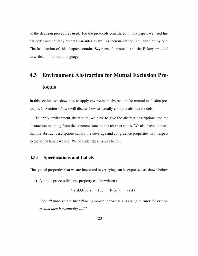
of the decision procedures used. For the protocols considered in this paper, we need lin-

ear order and equality on data variables as well as incrementation, i.e., addition by one.

The last section of this chapter contains Szymanski’s protocol and the Bakery protocol

described in our input language.

4.3 Environment Abstraction for Mutual Exclusion Pro-

tocols

In this section, we show how to apply environment abstraction for mutual exclusion pro-

tocols. In Section 4.5, we will discuss how to actually compute abstract models.

To apply environment abstraction, we have to give the abstract descriptions and the

abstraction mapping from the concrete states to the abstract states. We also have to prove

that the abstract descriptions satisfy the coverage and congruence properties with respect

to the set of labels we use. We consider these issues below.

4.3.1 Specifications and Labels

The typical properties that we are interested in verifying can be expressed as shown below.

• A single process liveness property can be written as

∀x.AG(pc[x] = try⇒ F(pc[x] = crit))

“For all processes x, the following holds: If process x is trying to enter the critical

section then it eventually will.”

123

•

∀x.AG(pc[x] = crit⇒ (crit /∈ env(x)))

“For all processes x the following invariant holds: If process x is in the critical

section, then no other process is in the critial section”

Consequently, the set of labels L again has two types of labels:

• pc[x] = L, and

• L ∈ env(x).

4.3.2 Abstract Descriptions

Technically, our descriptions reuse the predicates which occur in the control statements of

the protocol description. Let SL be the number of control locations in the program P . The

internal state of a process x can be described by a predicate of the form

pc[x] = L

where L ∈ 1..SL is a control location.

In order to describe the relations between the data variables of different processes we

collect all predicates EP1(x, y), . . . , EPr(x, y) which occur in the guards of the program.

From now on we will refer to these predicates as the inter-predicates of the program.

Since in most practical protocols, synchronization between processes involves only one or

two data variables, the number of inter-predicates is usually quite small. The relationship

124

between a process x and a process y is now described by a formula of the form

Ri(x, y).= ±EP1(x , y) ∧ . . . ∧ ±EPr(x , y)

where±EP i stands for EP i or its negation¬EP i. It is easy to see that there are 2r possible

relationships R1(x, y), . . . , R2r(x, y) between x and y. In the example of Figure 4.1, the

two relationship predicates R1 and R2 are visualized by full and dashed arrows.

Fact 3. The relationship conditions R1(x, y), . . . , R2r(x, y) are mutually exclusive.

Before we explain the descriptions ∆(x) in detail, let us first describe the most im-

portant building blocks for the descriptions, which we call environment predicates. An

environment predicate expresses that for process x we can find another process y which

has a given relationship to process x and a certain internal state. The environment predi-

cates thus have the form

∃y.y 6= x ∧Ri(x, y) ∧ pc[y] = j.

An environment predicate says the following: there exists a process y different from x

whose relationship to x is described by the EP predicates in Ri and whose internal

state is j. There are T := 2r × SL different environment predicates; we name them

E1(x), . . . , ET (x), and their quantifier-free matricesE1(x, y), . . . , ET (x, y). Note that each

Ek(x, y) has the form y 6= x ∧R(x, y) ∧ pc[y] = L.

Fact 4. If an environment process y satisfies an environment condition Ei(x, y), then it

cannot simultaneously satisfy any other environment condition Ej(x, y), i 6= j.

125

Proof. Each environment condition Ek(x, y) has the form y 6= x ∧ R(x, y) ∧ pc[y] = L.

Thus let

Ei(x, y).= y 6= x ∧ Ri(x, y) ∧ pc[y] = Li

and

Ej(x, y).= y 6= x ∧ Rj(x, y) ∧ pc[y] = Lj

Since Ei(x, y) and Ej(x, y) are different, either Ri(x, y) is different from Rj(x, y) or

Li 6= Lj .

In the former case, by Fact 3, Ri(x, y) and Rj(x, y) are mutually exclusive. Thus, if

process y satisfies Ei(x, y) then it cannot satisfy Ej(x, y).

In the latter case, if process y satisfies Ei(x, y) then the control location of process y

is Li. Since Li 6= Lj , process y cannot satisfy Ej(x, y).

Hence, in both the cases we have shown that if process y satisfies environment condi-

tion Ei(x, y) then it cannot satisfy any other environment condition Ej(x, y).

Fact 5. Given a state s and two different processes c and d, there exists a unique environ-

ment condition Ei(x, y) such that s |= Ei(c, d).

Proof. Let L be the control location of process d in state s. Thus, s |= pc[d] = L holds.

Given processes c and d, for each inter-predicate EPk(x, y) we have either s |= EPk(c, d)

or s 6|= EPk(c, d). Consider the formula

F (x, y).= y 6= x ∧ pc[y] = L ∧

∧

s|=EPk(c,d)

EPk(x, y) ∧∧

s 6|=EPk(c,d)

¬EPk(x, y).

126

Clearly, s |= F (c, d) by construction. Syntactically, F (x, y) is identical to a unique

environment condition. By Fact 4, processes c, d can satisfy at most one environment

condition.

Fact 6. Let Ei(x, y) be an environment condition and G(x, y) be a boolean formula over

the inter-predicates EP1(x, y), . . . , EPr(x, y) and predicates of the form pc[y] = L. Then

either Ei(x, y)⇒ G(x, y) or Ei(x, y)⇒ ¬G(x, y).

Proof. Since Ei(x, y) has the form pc[y] = j ∧ Rk(x, y) where Rk(x, y) is a min-term

over the inter-predicates EP1(x, y), . . . , EPr(x, y), Ei(x, y) enforces a unique truth value

for all atomic subformulas of G(x, y).

We are ready to return to the descriptions ∆(x). A description ∆(x) has the format

pc[x] = i ∧ ±E1(x) ∧ ±E2(x) ∧ · · · ∧ ±ET (x), where i ∈ [1..S].

Intuitively, a description ∆(x) gives detailed information on the internal state of process

x, and how the other processes are related to process x. Note the correspondence of ∆(x)

to the abstract state in Figure 4.1: the control location i determines the color of the central

circle, and the Ej determine the processes surrounding the central one.

Definition 4.3.1 (Abstraction Mapping). Let P (K), K > 1, be a concrete system and

p ∈ [1..K] be a process. The abstraction mapping αp induced by p maps a global state s

of P(K) to an abstract state 〈pc, e1, . . . , eT 〉 where pc = the value of pc[p] in state s and

for all ej we have ej = 1⇔ s |= Ej(p).

We will now prove the coverage and congruence conditions that let us apply environ-

ment abstraction.

127

Lemma 4.3.2. Consider a description ∆(x) and a label l(x). Then either ∆(x) ⇒ l(x)

or ∆(x)⇒ ¬l(x)

Proof. Consider first the case where l(x) .= pc[x] = L. Since ∆(x) is of the form

pc[x] = L ∧ ±E1(x) ∧ ±E2(x) ∧ · · · ∧ ±ET (x)

it is easy to see that, in this case, ∆(x) either ∆(x)⇒ l(x) or ∆(x)⇒ ¬l(x).

Consider the second case where label l(x) .= L ∈ env(x). Recall that L ∈ env(x) is

syntactic sugar for ∃y.y 6= x.pc[y] = L. The description ∆(x) is of the form

pc[x] = L ∧ ±E1(x) ∧ ±E2(x) ∧ · · · ∧ ±ET (x)

where each Ei(x) is of the form

∃y.y 6= x ∧ Rj(x, y) ∧ pc[y] = Li

Consider all those environment conditions Ei(x) of the form

∃y.y 6= x ∧ Rj(x, y) ∧ pc[y] = L

That is, those environment conditions that require the other process y to be in control

location L. Denote this set of environment conditions by EL.

Now

∆(x)⇒∨

Ei(x)∈EL

±Ei(x) (∗)

where the polarity of each Ei(x) in the consequent is exactly as in the description ∆(x).

Suppose at least one environment condition, say Ej(x), in EL appears un-negated in the

consequent of (∗). Then,

∆(x)⇒ Ej(x) (†)

128

Since Ej(x) is of the form

∃y.y 6= x ∧ Rk(x, y) ∧ pc[y] = L

it follows that

Ej(x)⇒ ∃y.y 6= x ∧ pc[y] = L.

Thus, we have

∆(x)⇒ ∃y.y 6= x ∧ pc[y] = L

in case at least one of the environment conditions in EL appears un-negated in ∆(x).

For the other case, suppose none of the environment conditions in EL appear unnegated

in ∆(x). Then we have

∆(x)⇒∧

Ei(x)∈EL

¬Ei(x)

or equivalently,

∆(x)⇒ ¬(∨

Ei(x)∈EL

Ei(x))

Now Ei(x) is of the form

∃y.y 6= x ∧ Rk(x, y) ∧ pc[y] = L

and where each Rk(x, y) is of the form

Rk(x, y).= ±EP1(x, y) ∧ . . . ∧ ±EPr(x, y)

Since the set of relation predicates Rk(x, y) is formed by taking all possible cubes over the

inter-predicates EP1(x, y), . . . , EPT (x, y) it follows that

∨Rk(x, y) = true

129

This means at least one of the relation predicates must be true. Assume without loss of

generality that Rp(x, y) is true. Let the corresponding environment condition from EL

which involves Rp(x, y) be Ep(x, y). Now

∆(x)⇒ ¬(∨

Ei(x)∈EL

Ei(x))

which implies

∆(x)⇒ ¬(Ep(x))

that is

∆(x)⇒ ∃y.y 6= x ∧ Rp(x, y) ∧ pc[y] = L

Since Rp(x, y) is true

Ep(x).= ∃y.y 6= x ∧ pc[y] = L

So we have

∆(x)⇒ ∃y.y 6= x ∧ pc[y] = L

or equivalently

∆(x)⇒ ¬l(x)

Thus, in case none of the environment conditions in EL appear unnegated in ∆(x), ∆(x)⇒

¬l(x). Hence either ∆(x) ⇒ l(x) or ∆(x) ⇒ ¬l(x) and the lemma is proved. Note that,

this lemma establishes the congruence property described in Section 2.2.

Remark 11. Consider the full set of descriptions

pc[x] = L ∧ ±E1(x) ∧ ±E2(x) ∧ · · · ∧ ±ET (x), where L ∈ [1..S].

130

Given any concrete state s and process c in a system P(K) it is clear that s |= ∆(c) for

some description ∆(x). This is true simply because we take every possible conjunction

of the predicates E1(x), . . . , ET (x) with every possible predicate pc[x] = L. Thus, the

coverage condition discussed in Section 2.2 holds for the set of descriptions given above.

The other property required to make environment abstraction sound, namely the con-

gruence property is established by the above lemma. Thus, for the chosen set of abstract

descriptions and labels, environment abstract is sound.

We will now represent descriptions ∆(x) by tuples of values, as usual in predicate

abstraction. The possible descriptions (∗) only differ in the value of the program counter

pc[x] and in where they have negations in front of the E(x) predicates. Denoting negation

by 0 and absence of negation by 1, every description ∆(x) can be identified with a tuple

〈pc, e1, . . . eT 〉 where pc is a control location, and each ei is a boolean variable.

Example 4.3.3. Consider again the protocol shown in Example 4.2.1. There is only

one inter-predicate EP1(x, y).= t[x] 6= t[y]. Thus, we have two possible relationship

conditions R1(x, y).= t[x] = t[y] and R2(x, y)

.= t[x] 6= t[y]. Consequently, we have 6

different environment predicates:

E1(x).= ∃y 6= x.pc[y] = 1 ∧ R1(x, y) E4(x)

.= ∃y 6= x.pc[y] = 1 ∧ R2(x, y)

E2(x).= ∃y 6= x.pc[y] = 2 ∧ R1(x, y) E5(x)

.= ∃y 6= x.pc[y] = 2 ∧ R2(x, y)

E3(x).= ∃y 6= x.pc[y] = 3 ∧ R1(x, y) E6(x)

.= ∃y 6= x.pc[y] = 3 ∧ R2(x, y)

The abstract state then is a 7-tuple 〈pc, e1, . . . , e6〉 where pc refers to the internal

state of the reference process x. For each i ∈ [1..6], the bit ei tells whether there is an

131

environment process y 6= x such that the environment predicate Ei(x) becomes true. 2

We build the abstract model PA exactly as in Section 2.2. Since the congruence and

coverage conditions hold for the set of descriptions and labels we have chosen, we have

the following corollary of Theorem 2.2.4:

Corollary 3 (Soundness of Abstraction). LetP(N) be a parameterized mutual exclusion

system and PA be its abstraction. For an indexed property ∀x.Φ(x), where Φ(x) is a

control condition, we have

PA |= Φ(x)⇒ ∀K.P(K) |= ∀x.Φ(x).

4.4 Extensions for Fairness and Liveness

The abstract model that we have described, while sound, might be too coarse in practice

to be able to verify liveness properties. The reason is two fold:

(i) Spurious Infinite Paths. Our abstract model may have infinite paths which cannot

occur in any concrete system. Figure 4.2 shows one such instance, where a self-loop

in the abstract model leads to a spurious infinite path. The two concrete states s1

and s2, such that s1 transitions to s2, map to the same abstract state s, leading to

a self-loop involving s. This self-loop can lead to a spurious infinite path. Such

spurious paths hinder the verification of liveness properties.

132

Figure 4.2: Process 7 changes its internal state, but the abstract state is not affected. Thus, there is a self-

loop around the abstract state. The abstract infinite path consisting of repeated executions of this loop has

no corresponding concrete infinite path.

(ii) Fairness Conditions. Liveness properties are usually expected to hold under some

fairness conditions. A typical example of a fairness condition is that every process

x must leave the critical section a finite amount of time after entering it. This is

expressed formally by the fairness condition pc[x] 6= crit. In this work, we will

consider fairness conditions pc[x] 6= L, where L is a control location. Liveness

properties are then expected to hold on fair paths: an infinite path in a concrete

system P(K), K > 1 is fair only if, for each process i, the fairness condition

pc[i] 6= L holds infinitely often.

133

Monitor Processes for Liveness

To handle these situations, we adapt a method developed by Pnueli et al. [66] in the

context of counter abstraction to our environment abstraction. The extension to handle

liveness essentially consists of adding monitor processes. We first augment the concrete

system P(K) by adding monitor processes M(1), . . . ,M(K) where each M(i) has two

sets of variables

• variables fromi1, . . . , from

iT where T is the number of different environments, and

• variables toi1, . . . , toiT where T is the number of different environments.

Intuitively, the fromi and toi variables keep track of the processes coming and going

out of the environments E1(i), . . . , ET (i) as viewed from process i.

Updating Monitor Variables

Suppose the system P(K) is initially in state s1 and some process j changes its state

resulting in state s2 for system P(K). Monitor process M(i) then updates its variables as

follows.

• Case 1: A process j 6= i changes its state

By Fact 4, we have uniquely defined environment predicates Ep(i) and Eq(i) such

that s1 |= Ep(i, j) and s2 |= Eq(i, j). Thus monitor process M(i) sets fromip =

true and toiq = true in state s2. The rest of the fromi and toi variables are set to

false in state s2.

134

• Case 2: j = i and the process changes its state using update transition

For each environment condition Ep(i) such that there is a process y satisfyingEp(i, y)

in s1, fromip = true in state s2. For each environment condition Ep(i) such that

there is a process z satisfying Ep(i, z) in s2, toip = true in state s2. In all other

cases, the fromi and toi variables in s2 are false.

• Case 3: j = i and the process changes its state using a guarded transition

In this case, all the fromi and toi variables in s2 are false.

Denote the system obtained by augmentingP(K) with monitor processesM(1), . . . ,M(K)

byPM(K). The states ofPM(K) are given by tuples of the form 〈L1, . . . ,LK,M1, . . . ,MK〉

where Li is denotes local state of process i andMi denotes the local state of the monitor

process M(i). The augmented abstract states, given by tuples of the form

〈pc, e1, . . . eT , from1, . . . , fromT , to1, . . . , toT 〉, carry monitor information for reference

process unchanged.

Definition 4.4.1 (Abstraction Mapping). Let PM(K), K > 1, be an augmented system

and p ∈ [1..K] be a process. The abstraction mapping αp induced by p maps a global state

s of PM(K) to an abstract state 〈pc, e1, . . . , eT , from1, . . . , fromT , to1, . . . , toT 〉 where

• pc = the value of pc[p] in state s

• for all ej we have ej = 1⇔ s |= Ej(p).

• ∀j. fromj = frompj

• ∀j. toj = topj

135

Intuitively, the from, and to variables keep track of the immediate history of an ab-

stract state, that is, the last step by which the abstract state was reached.

Example 4.4.2. Referring to Figure 4.2, suppose process 7 in state s1 satisfies the environ-

ment condition Ei(1, 7). Then, in the new augmented abstract state, variable fromi will

be set to true to indicate that a process satisfying environment condition Ei(1) made the

move. Similarly, suppose that in the new concrete state s2, process 7 satisfies the environ-

ment condition Ej(1, 7). Then in the new augmented abstract state, the variable toj is set

true to indicate that after the transition process 7 satisfies the new environment condition

Ej(1).

Remark 12. Note that the abstract model does not retain the id of the process which was

responsible for the transition (process 7 in this case). The abstract model only retains the

environment predicates satisfied by the process before and after the transition. We are

doing this for two reasons:

• During abstraction, all the processes except the reference process lose their identi-

ties.

• Remembering the environment predicate satisfied by the active process will give us

a sufficiently precise abstraction to verify the properties of interest.

To recapitulate, using the from and to variables we are able to keep track of the last step

of the route by which an abstract state was reached.

For an augmented abstract state s, we denote its projection consisting of only the pc

and ei variables by π(s). The following notation is also useful: let s1, s2 be two concrete

136

states in a system P(K) such that there is a transition from s1 to s2. Denote by s1 s2 the

index of the process whose local transition lead to the global transition from s1 to s2, e.g.

process 7 in Figure 4.2. Recall that in an asynchronous system, only one process at a time

changes its state, i.e., for each global transition, there exists a single process causing the

transition.

The augmented abstract model PAa.= (SA

a , IAa , R

Aa , L

Aa ) of the augment parameterized

system PM(K) is defined as in Section 2.5.2.

Note that coverage and congruence conditions for the augmented abstract descriptions

are trivial to establish given that the original abstract descriptions satisfy both conditions.

It follows from Section 2.5.2 that adding the additional monitor information does not affect

the soundness of our abstract model. Thus, we have PAa |= Φ(x)⇒ PM(K) |= ∀x.Φ(x)

where Φ(x) is a control condition.

Corollary 4 (Soundness of Augmented Abstraction). Let P(N) be a parameterized

system and PM(N) be an augmentation of P(N) with monitor processes as described

above and PAa be its augmented abstraction. For an indexed property ∀x.Φ(x), where

Φ(x) is a control condition we have

PAa |= Φ(x)⇒ ∀K.PM(K) |= ∀x.Φ(x) ⇒ ∀K.P(K) |= ∀x.Φ(x)

4.4.1 Abstract Fairness Conditions

We will now show how to deal with the two problems mentioned in the beginning of this

section, i.e., (i) spurious paths and (ii) fairness conditions.

137

Eliminating Spurious Infinite Paths.

Recall from the example in Figure 4.2 that due to the abstraction there may exist infinite

spurious paths that do not have any corresponding concrete paths, in particular such paths

where fromi is true infinitely often but toi is not. Such a path cannot correspond to any

concrete path because:

• By definition, the variable fromi is true if a process having satisfied Ei(x) in the

previous state, does not satisfy Ei(x) in the current state.

• By definition, the variable toi is true if a process having satisfied Ej(x) in the previ-

ous state, does satisfy Ei(x) in the current state.

• Each concrete system has only a finite number of processes.

• Thus, for a finite number of processes to make fromi true infinitely often, it is

necessary for toi to be true infinitely often as well.

Therefore, to eliminate the spurious infinite paths arising from loops described above, we

add for each i ∈ [1..T ] a compassion condition [66] 〈fromi, toi〉 which says if fromi =

true holds infinitely often in a path, then toi = true must hold infinitely often as well.

We will denote this set of fairness conditions by F1.

Adding Abstract Fairness Conditions.

Assume that in the concrete model each process has a fairness condition of the form pc 6=

L. This means that a process is not allowed to stay at control locationL forever. To abstract

138

the concrete fairness condition we have to find two sets of abstract fairness conditions, one

for the reference process IA and the other for the environment processes.

Fairness conditions for the environment processes. The abstract model maintains the

properties of the environment processes only in terms of the environment predicates. Thus,

the concrete fairness conditions on the environment processes have to be translated to

fairness conditions involving the environment predicates.

More precisely, given a fairness condition pc 6= L, we need to consider those environ-

ment conditions that require the environment process to be in control location L, i.e., those

environment conditions Ei(x, y) where Ei(x, y).= Rj(x, y) ∧ pc[y] = L. For each such

Ei(x , y) we add the fairness condition

¬(fromi = false ∧ ei = 1).

This condition excludes the cases where along an infinite path, the set of processes sat-

isfying the environment condition Ei(x, y) is non-empty (i.e., ei = 1) and none of these

processes ever changes its state (i.e., fromi = false). We will denote this set of fairness

conditions by F2

Fairness conditions for the reference process. The abstract fairness condition correspond-

ing to the reference process is given by pc 6= L. This expresses the requirement that the

control location of the reference process is not L infinitely often. We will denote this set

of fairness conditions by F3.

139

4.4.2 Soundness in the Presence of Fairness Conditions

Now we will show that adding these fairness conditions do not rule out any legitimate

paths in the abstract model. Thus, the augmented abstracted model will be sound.

We are usually interested in verifying single index liveness properties of the form

∀x.AG(φ(x)→ Fψ(x)).

For example, for mutual exclusion protocols, the standard liveness property, which

says if process is trying to get into the critical section it eventually will, can be written as

∀x.AG(pc[x] = try→ F(pc[x] = crit)).

The following theorem claims that, for single index liveness properties, the augmented

abstract model that we constructed is sound.

Theorem 4.4.3 (Soundness of Abstraction). Let P(K) be a parameterized system with

fairness constraint pc 6= L and PAa be its augmented abstraction using the abstract fair-

ness and compassion conditions. Given the single-indexed liveness property ∀x.Φ(x),

PAa |= Φ(x) under the abstract fairness conditions implies P(K) |= ∀x.Φ(x) under the

concrete fairness condition.

The augmented abstraction thus obtained is precise enough to prove liveness properties

for the two mutual exclusion protocols we considered. The following section gives a proof

of the soundness theorem.

140

4.4.3 Proof of Soundness

Given concrete fairness condition pc[x] 6= L, the augmented abstract model has three sets

of fairness conditions:

F1. For each i ∈ [1..T ], the compassion condition 〈fromi, toi〉 saying that if fromi =

true infinitely often along an abstract path then toi = true infinitely often as well.

F2. The fairness conditions ¬(fromi = true∧ ei = 1) for each i such that the environ-

ment condition Ei(x, y) requires process y to be in control location L.

F3. The fairness condition pc 6= L requiring that the reference process satisfies the

concrete fairness condition pc[x] 6= L.

The proof of Theorem 4.4.3 relies on the following lemma.

Lemma 4.4.4. Let P(K) be a concrete system with process c and let σ .= g0, g1, . . . be a

fair path under the fairness constraint pc[x] 6= L. Then the augmented abstract model PAa

has a path σ .= g0, g1, . . . such that

1. for each i ≥ 0, π(gi) = αc(gi), and

2. the abstract fairness conditions F1, F2, F3 hold for σ.

Proof. The lemma claims that corresponding to every concrete fair path and a given ref-

erence process c there is an abstract fair path in the augmented abstract model. In other

words, our abstract fairness conditions do not remove any fair paths.

141

Given a concrete fair path σ of system P(K) we construct an abstract fair path σ as

follows:

• For the first state g0 we require π(g0) = αc(g0), and the fromi and toi variables can

have any value.

• For each gi, i > 0 we require αc(gi) = π(g1), and the toi, and fromi are set accord-

ing to the definition of the augmented abstract transition relation in Section 4.4.

Thus, item 1 of the lemma is satisfied by construction. The fact that σ is a valid trace

in the abstract model also follows by construction.

We will now show that if σ is a fair path then σ satisfies the abstract fairness conditions

as well. We consider the different ways in which σ might fail to satisfy the abstract fairness

conditions and argue that each case leads to a contradiction.

Violation of F1. Assume towards a contradiction that σ violates the compassion condition

〈fromk, tok〉 for some k ∈ [1..T ], i.e., there exists an i ≥ 0 such that

• fromk is true infinitely often in states gi, gi+1, . . . (†)

• but tok = false in all the states gi, gi+1, . . . (*)

There are two cases in which fromk holds true in a certain state gl:

(a) A process y satisfying enviroment condition Ek(c, y) in gl−1 moves to a new envi-

ronment in gl.

142

(b) In state gl−1, there is a process y satisfying the environment condition Ek(c, y), and

the reference process c makes an update transition from gl−1 to gl.

For fromk to be true infinitely often, either case (a) or case (b) has to hold infinitely

often. We will show that both cases lead to a contradiction. First assume case (a). As there

are only a finite number of processes, fromk being true inifinitely often requires tok to be

true infinitely often as well. This contradicts (*).

In case (b) the fromk is true in a state gl because the reference process made an update

transition and there was process y satisfying the environment Ek(c, y) in state gl−1. After

such an update transition we again have two cases:

(b.1) There is a process y satisfying the condition Ek(c, y) in state gl, i.e., ek is 1 in gl.

In this case tok is set to true by our definition of the augmented abstract transition

relation in Section 4.4, or

(b.2) there is no process y satisfying the condition Ek(c, y) in state g1 i.e., ek = 0.

The former case (b.1) immediately contradicts the assumption (*). In the latter case

(b.2), if ek continues to be 0, then, by definition, fromk cannot be true again. This

contradicts the assumption (†).

Thus, we have proved that the compassion condition 〈fromi, toi〉 cannot be violated

in the abstract trace σ.

Violation of F2. Assume towards a contradiction that σ violates the fairness condition

¬(fromk = false ∧ ek = 1) where the environment condition Ek(x, y) requires process

y to be in control location L. That is, there exists an i ≥ 0 such that gj |= fromk =

143

false ∧ ek = 1 for all j ≥ i. In other words, in the concrete trace in all the states

gj, gj+1, . . . of the concrete trace there is a process y satisfying the environment condition

Ek(c, y), and this process y never leaves the environment corresponding toEk(x, y). Since

Ek(x, y) requires process y to be in control location L, process y violates the concrete

fairness condition pc[slf] 6= L, and thus, the assumption of the lemma.

Violation of F3. Assume towards a contradiction that σ violates the fairness condition

pc 6= L, i.e., there is an i ≥ 0 such that for all gj, j > i, gj |= pc = L holds. This is

possible only if process c stays in control location L after concrete state gi, thus violating

the concrete fairness condition, and thus, the assumption of the lemma.

We see that in all the three cases we are led to a contradiction. Consequently, the

abstract trace σ does not violate any abstract fairness conditions.

Theorem 4.4.3. Consider a single index liveness property ∀x.AG(φ(x) → Fψ(x)). As-

sume that

PAa |= Φ(x)

under abstract fairness conditions, and assume towards a contradiction that there is a fair

path σ.= g0, g1, . . . in system P(K) such that σ 6|= φ(c) → Fψ(c) for some process

c. Thus, there exists an i ≥ 0 such that gi |= φ(c) and gj 6|= ψ(c) for all j ≥ i. By

Lemma 4.4.4 there is a fair abstract path σ .= g0, g1, . . . such that for all k, π(gk) = αc(gk).

By definition, gi |= φ(x) and for all j ≥ i, gj 6|= ψ(x). Thus, there is a fair path σ in the

abstract model PAa that violates the liveness property Φ(x), contradicting our assumption

that PAa |= Φ(x). This completes our proof.

144


We have thus far presented the theoretical description of the abstract model and the prop-

erties it satisfies. We have not described how to actually obtain such an abstract model

from a given parameterized system. In this section, we will show how to construct the

abstract model.

Computing the abstract model is evidently complicated by the fact there is an infinite

number of concrete systems. Further, it is well known that in predicate abstraction and

related methods, computing the exact abstract model is computationally very expensive.

Instead of finding the most precise abstract model, we find an over-approximation of the

abstract model. We consider each concrete transition statement of the program separately

and over-approximate the set of abstract transitions it can lead to. The union of these

sets will be the abstract transition relation. A concrete transition can either be a guarded

transition or an update transition. Each transition can be executed by the reference process

or one of the environment processes. Thus, there are four cases to consider:

Active process is . . . guarded transition update transition

. . . reference process Case 1 Case 2

. . . environment process Case 3 Case 4

We will show how we abstract in each of these cases and argue why the computed

abstract transition is an over-approximation. Before we begin we recall the following

facts:

Fact 7. For any two environment predicates Ei(x , y) and Ej(x , y), i 6= j Ei(x , y) ⇒

¬Ej(x , y).

145

Fact 8. Given any formula G(x , y) involving inter-predicates EP 1(x , y), . . . , EPr(x , y)

either Ei(x , y)⇒ ¬G(x , y) or Ei(x , y)⇒ G(x , y).

We now introduce some useful notation. The environment condition Ei(x, y).= y 6=

x ∧Rj(x, y) ∧ pc[y] = L will be denoted by E(j,L)(x, y). The variables and formulas cor-

responding to this environment condition are referred to using the same subscript j, L,

e.g., the corresponding environment predicate is referred to as E(j,L)(x) and the corre-

sponding abstract variable is e(j,L). The set of all environment conditions E(j,L)(x, y) is

referred to as EL.

4.5.1 Case 1: Guarded Transition for Reference Process

Consider first the case of guarded transitions being executed by the reference process.

Consider the guarded transition statement tG:


Suppose the reference process is executing this guarded transition statement. If at

least one of the environment processes contradicts the guard G then the reference process

transitions to control location L3, i.e., the else branch. Otherwise, the reference process

goes to L2. We will now formalize the conditions under which the if and else branches are

taken.

Definition 4.5.1 (Blocking Set for Reference Process). Let G.= ∀otr 6= slf.G(slf, otr) be

146

a guard. We say that an environment condition Ei(x , y) blocks the guard G if Ei(x , y)⇒

¬G(x , y). The set Bx(G ) of all indices i such that Ei(x , y) blocks G is called the blocking

set of the reference process for guard G .

Note that by Fact 6, either Ei(x , y) ⇒ ¬G(x , y) or Ei(x , y) ⇒ G(x , y) for every

environment Ei(x , y). The intuitive idea behind the definition is that Bx(G ) contains the

indices of all environment conditions which enforce the else branch.

We will now explain how to represent the guarded transition tG in the abstract model:

we introduce an abstract transition from s1 = 〈pc, e1, .., eT , from1, .., fromT , to1, .., toT 〉

to s2 = 〈pc′, e1, .., eT , from′1, .., from

′T , to

′1, .., to

′T 〉 if

GR1. pc = L1, i.e., the reference process is in location L1,

GR2. one of the following two conditions holds:

• Then Branch: ∀i ∈ Bx(G ). (ei = 0) and pc′ = L2, i.e., the guard is true and

the reference process moves to control state L2.

• Else Branch: ¬∀i ∈ Bx(G ). (ei = 0) and pc′ = L3, i.e., the guard is false and

the reference process moves to control state L3.

GR3. and all the variables from′1, .., from

′T and to′1, .., to

′T are false, expressing that

none of the environment processes changes its state.

Together, these three conditions can be viewed as an transition invariant Ix(tG) be-

tween the current and the next abstract states. The following fact shows that the set of

147

abstract transitions represented by Ix(tG) is indeed an over-approximation of the set of

abstractions that tG gives rise to.

Lemma 4.5.2. Let s1 be a state in a concrete system P(K), and suppose that a process

c executes a guarded transition tG which leads to state s2. Then the abstract states s1.=

αc(s1) and s2.= αc(s2) satisfy the invariant Ix(tG).

Proof. Assume there is a guarded transition tG from state s1 to s2 with the reference pro-

cess c as the active process. There are two cases to consider:

• The concrete guard was true in state s1 and process c’s new control location in

state s2 is L2. By Fact 6, each environment condition Ei(x, y) either implies the

guard condition G(x, y) or its negation. Any process y satisfying an environment

Ej(x, y), j ∈ Bx(G ) would block the guard G(c, y). In other words, for the then

branch to be taken, in state s1 every concrete process y 6= c must have satisfied only

environment conditions which are not mentioned in the blocking set Bx(G ). Thus,

the condition ∀i ∈ Bx(G ).ei = 0 is true in s1 and the abstract model transitions to

state s2.

• The concrete guard was false in state s1 and process c’s new control location in state

s2 is L3. By Fact 6, each environment condition Ei(x, y) either implies the guard

condition G(x, y) or its negation. For the else-branch to be taken, there must be at

least one process y in state s1 satisfying an environmentEj(x, y), j ∈ Bx(G ) so that

the guard G(c, y) evaluates to false. Thus, the abstract condition ∀i ∈ Bx(G ).ei = 0

is false for s1, and the abstract model still transitions to state s2.

148

4.5.2 Case 2: Guarded Transition for Environment Processes

Suppose that the guarded transition tG


is executed by a concrete process y satisfying the environment condition E(i,L1)(x, y).

The active process thus switches from environment condition E(i,L1)(x, y) to environment

condition E(i,L2)(x, y) or E(i,L3)(x, y). Note that in a guarded transition, only the pc of the

active process changes.

We will now define a blocking set for this environment condition E(i,L1)(x, y) as fol-

lows. The difference from Definition 4.5.1 is that the guard for process y can be blocked

either by the reference process or by another environment process. Therefore we need to

distinguish two cases in the definition.

Definition 4.5.3 (Blocking Set for Environment E(i,L1)(x, y)). Let G (slf) = ∀otr 6=

slf.G(slf, otr) be a guard. We say that

1. An environment conditionEj(x, z) blocks the guard for process y satisfyingE(i,L1)(x, y)

if

E(i,L1)(x, y) ∧ Ej(x, z)⇒ ¬G(y, z).

Let B1(i,L1)(G) be the set of all such indices j.

149

2. The control location L of the reference process x blocks the guard for process y

satisfying E(i,L1)(x, y) if

E(i,L1)(x, y) ∧ pc[x] = L⇒ ¬G(y, x).

Let B2(i,L1)(G) be the set of all such control locations L.

Note that we consider the guards G(y, z) and G(y, x) because y is the active process,

i.e., y executes the transition. We define the abstract guard G i for guard G (slf) .= ∀otr 6=

slf.G(slf, otr) and the environment condition Ei(x, y) as follows:

∀j ∈ B1(i,L1)(G ).(ej = 0) ∧ pc /∈ B2

(i,L1)(G ).

Since the transition starts in control location L1 and the active process is an environment

process, we will describe the abstract transition invariant I i,L1y (tG) for each E(i,L1)(x, y) ∈

EL1 by a list of conditions as in Case 1. The abstract transition invariant for Case 2 will

then be

Iy(tG).=

∨

E(i,L1)(x,y)∈EL1

I i,L1y (tG).

Consider one such E(i,L1)(x, y) ∈ EL1 . The abstract transition relation I i,L1y (tG) has a

transition from s = 〈pc, e1, . . . , eT , from1, . . . , fromT , to1, . . . , toT 〉

to s′ = 〈pc′, e′1, . . . , e′T , from

′1, . . . , from

′T , to

′1, . . . , to

′T 〉 if the following conditions hold:

GE1. e(i,L1) = 1, that is, there is a process satisfying environment condition E(i,L1)(x, y).

GE2. from′(i,L1) = true, that is, the active process switches from environment condition

E(i,L1)(x, y) to some other environment condition.

150

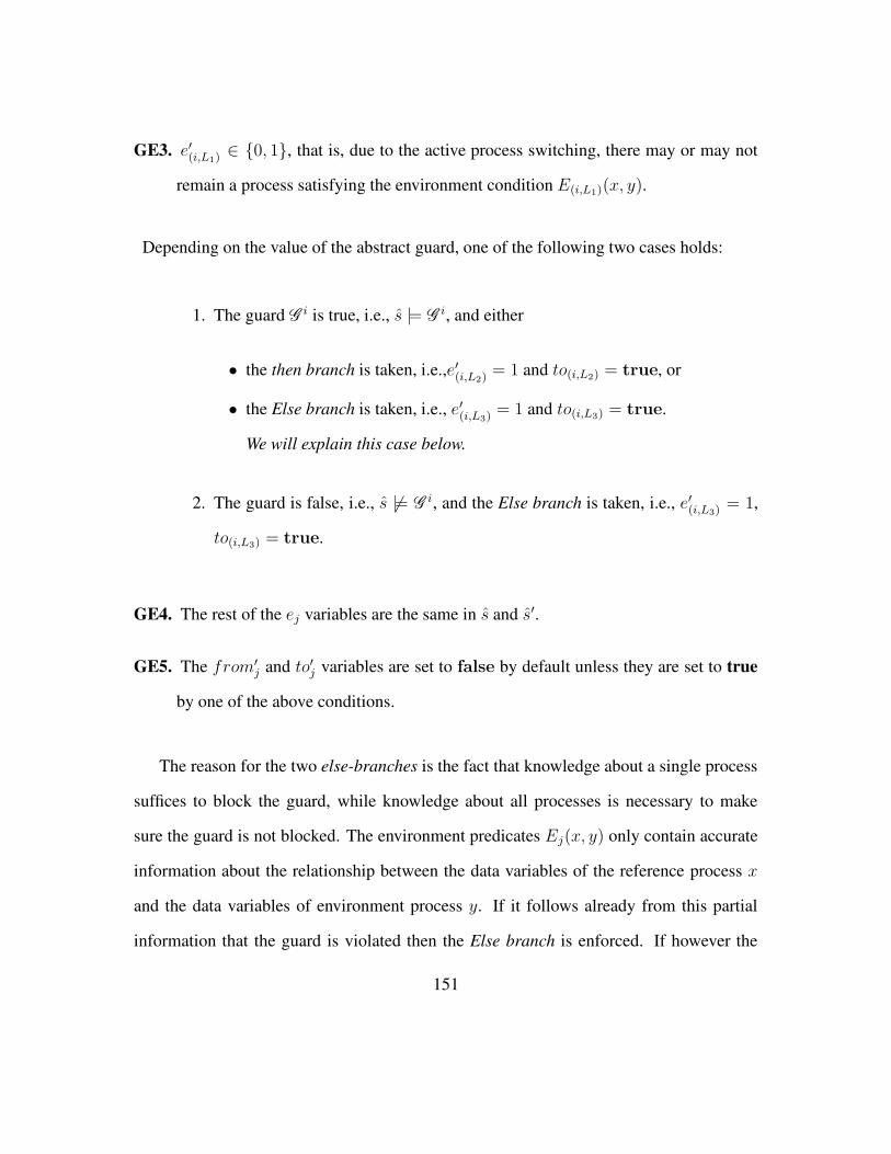
GE3. e′(i,L1) ∈ 0, 1, that is, due to the active process switching, there may or may not

remain a process satisfying the environment condition E(i,L1)(x, y).

Depending on the value of the abstract guard, one of the following two cases holds:

1. The guard Gi is true, i.e., s |= G

i, and either

• the then branch is taken, i.e.,e′(i,L2) = 1 and to(i,L2) = true, or

• the Else branch is taken, i.e., e′(i,L3) = 1 and to(i,L3) = true.

We will explain this case below.

2. The guard is false, i.e., s 6|= Gi, and the Else branch is taken, i.e., e′(i,L3) = 1,

to(i,L3) = true.

GE4. The rest of the ej variables are the same in s and s′.

GE5. The from′j and to′j variables are set to false by default unless they are set to true

by one of the above conditions.

The reason for the two else-branches is the fact that knowledge about a single process

suffices to block the guard, while knowledge about all processes is necessary to make

sure the guard is not blocked. The environment predicates Ej(x, y) only contain accurate

information about the relationship between the data variables of the reference process x

and the data variables of environment process y. If it follows already from this partial

information that the guard is violated then the Else branch is enforced. If however the

151

guard Gi is true, this may be due to lack of information in the abstract predicates, and we

over-approximate the possible abstract transitions.

Note that Case 2 is different to Case 1, because, in Case 1, the reference process makes

the guarded transition, while in Case 2, an environment process makes the transition. In

case of the reference process, our abstraction maintains the relationship of its data variables

to the other variables. In case of an environment process, we only know the relationship

of its data variables to the reference process.

Lemma 4.5.4. Let s1 be a state in a concrete system P(K), and let c be a process used

as reference process. Suppose that a process d 6= c executes a guarded transition tG that

leads to state s2. Then the abstract states αc(s1) and αc(s2) satisfy the invariant Iy(tG).

Proof. This follows directly from the construction of the transition invariant I y(tG).

4.5.3 Case 3: Update Transition for Reference Process

Consider the case where the reference process is executing an update transition tU :


goto L2

Recall that each process has data variables u1, . . . , ud. We denote the next state value

of each variable um by u′m.

152

When the reference process x changes the value of its data variables, the valuations of

the environment predicates E1(x) . . . ET (x) will change. For a process y satisfying envi-

ronment conditionEi(x, y) we need to figure out the possible new environment conditions

Ej(x, y) that y might satisfy after the reference process x has executed the update transi-

tion. The set of possible new environment conditions for process y is called the outset Oi

for condition Ei(x, y). (Technically, the outset is the set of the indices of these environ-

ment conditions.) We will now explain how to compute the outset.

Denote by T(x, y) the formula

T (x, y) ∧ u′k[x] := φ(y) ∨ ¬T (x, y) ∧ u′k[x] := uk[x].

We call T(x, y) the update formula. Given the update formula we find what possible

inter-predicates involving u′k[x], uk[y] can be true. Formally, the set C1(uk) of these inter-

predicates is given by all formulas uk[x] ≺ uk[y] where ≺∈ <,>,= such that

u′k[x] ≺ uk[y] ∧ T(x, y) is satisfiable.

Thus, C1uk

contains all possible ways uk[x] and uk[y] can relate to each other after the

update. The possible relationships between uk[x] and uk[y] might change again when, in

the course of evaluating the update transition, x repeatedly updates its uk value by looking

at other processes.

Suppose x looks at another process z and updates its uk[x] value again. We now find

the set C2(uk) of possible relationships between uk[x] and uk[y] after the new update

involving process z under the assumption that a relation from C1(uk) holds before the

update.

153

Thus, the new set C2(uk) of relationships is given by all formulas uk[x] ≺ uk[y] where

≺∈ <,>,=, such that

u′k[x] ≺ uk[y] ∧ T(x, z) ∧ ψ(x, y) is satisfiable and ψ(x, y) ∈ C1(uk).

Note that C1(uk) ⊆ C2(uk) because the definition of T(x, z) allows the possibility that

the value of uk[x] remains unchanged. We similarly compute sets C3(uk), C4(uk) . . . until

a fixpoint is reached. Since the number of possible inter-predicates is finite, a fixpoint

always exists; for simple inter-predicates involving <,>, and =, the fixpoint computation

takes three iterations at the most. We denote this fixpoint by C(uk).

In the environment condition Ei(x, y), let θ be the inter-predicate that describes the

relation between uk[x] and uk[y]. Consider the set of environment conditionsEj(x, y) that

are obtained from Ei(x, y) by replacing θ by a formula in the fixpoint C(uk) – the indices

of these environment conditions constitute the outset Oi of Ei(x, y). Correspondingly, the

inset Ik ⊆ 1..T for environment condition Ek(x, y) consists of all j such that k ∈ Oj.

We denote the abstract transition invariant corresponding to the concrete update tran-

sition tU by Ixup(tU). Ixup(tU) has a transition from the abstract state

s = 〈pc, e1, . . . , eT , from1, . . . , fromT , to1, . . . , toT 〉 to the abstract state

s′ = 〈pc′, e′1, . . . , e′T , from

′1, . . . , from

′T , to

′1, . . . , to


UR1. pc = L1, i.e., the reference process is in control location L1 before the transition.

UR2. pc′ = L2, i.e., the reference process moves to control location L2.

UR3. ∀k ∈ [1..T ].(ek = 1 ⇒ ∃j ∈ Ok.e′j = 1), i.e., if there was a process in environ-

ment Ek(x) before the transition then there must be a process in one of the outset

154

environments Ok of Ek(x, y) after the transition.

UR4. ∀j ∈ Ik.(ej = 0 ⇒ e′k = 0), i.e., if there is no process satisfying the inset environ-

ments Ik of environment Ek(x, y) before the transition then after the transition there

can be no process in environment Ek(x, y).

UR5. ∀k ∈ [1..T ].(e′k = 1 ⇔ to′k = true). The variable to′k indicates if after the

transition there is a process satisfying Ek(x, y).

UR6. ∀k ∈ [1..T ].(ek = 1 ⇔ from′k = true). The variable from′

k indicates if before

the transition there is a process satisfying Ek(x, y).

Lemma 4.5.5. Let s1 be a state in a concrete system P(K), and suppose that a process c

executes an update transition tU which leads to state s2. Then the abstract states αc(s1)

and αc(s2) satisfy the invariant Ixup(tU).

Proof. This follows directly from the construction of the invariant Ixup(tU).

4.5.4 Case 4: Update Transition for Environment Processes

This case is quite similar to Case 3. Recall that E(i,L1)(x, y) denotes the environment

condition y 6= x ∧ Ri(x, y) ∧ pc[y] = L1. Consider the case where a generic process y

satisfying environment E(i,L1)(x, y) is executing an update transition tU :

155


goto L2

After the update transition process y will have a new control location and also the rela-

tionship of its data variables to those of the reference process xwill have changed. The out-

set O(i,L1) for environmentE(i,L1)(x, y) will consist of all those environmentsE(j,L2)(x, y)

that process y may satisfy after the update transition. To compute the outset O(i,L1) we

proceed as follows. As in the previous case, we find a fixpoint C(uk) that contains the

possible relationships between uk[x] and uk[y]. The initial set of relationships C1(uk) is

the set of all uk[x] ≺ uk[y], ≺∈ <,>,= such that

T(y, x) ∧ uk[x] ≺ u′k[y] is satisfiable

where T(y, x) is the update condition as defined in Section 4.5.3. Note that we consider

T(y, x) (and not T(x, y) as in the previous section) because y is the active process. As y

updates its uk variable repeatedly, the relationship between uk[x], uk[y] will also change.

To compute all the possible relationships we use an approach similar to the fixpoint com-

putation in Case 3. Thus, we find the set C2(uk) of all uk[x] ≺ uk[y], ≺∈ <,>,= such

that

T(y, z) ∧ uk[x] ≺ u′k[y] ∧ ψ(x, y) is satisfiable

where ψ(x, y) ∈ C1(uk). We similarly compute C3(uk), C4(uk), . . . until we reach a

fixpoint C(uk).

In the environment conditionE(i,L1)(x, y), let θ be the inter-predicate that describes the

relation between uk[x] and uk[y]. Consider the set of environment conditions E(j,L2)(x, y)

156

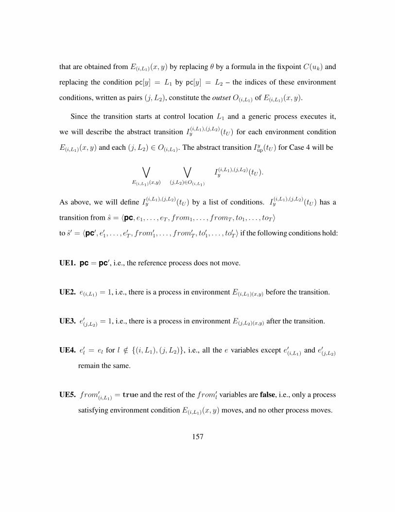
that are obtained from E(i,L1)(x, y) by replacing θ by a formula in the fixpoint C(uk) and

replacing the condition pc[y] = L1 by pc[y] = L2 – the indices of these environment

conditions, written as pairs (j, L2), constitute the outset O(i,L1) of E(i,L1)(x, y).

Since the transition starts at control location L1 and a generic process executes it,

we will describe the abstract transition I(i,L1),(j,L2)y (tU) for each environment condition

E(i,L1)(x, y) and each (j, L2) ∈ O(i,L1). The abstract transition Iyup(tU ) for Case 4 will be

∨

E(i,L1)(x,y)

∨

(j,L2)∈O(i,L1)

I(i,L1),(j,L2)y (tU).

As above, we will define I (i,L1),(j,L2)y (tU) by a list of conditions. I

(i,L1),(j,L2)y (tU) has a

transition from s = 〈pc, e1, . . . , eT , from1, . . . , fromT , to1, . . . , toT 〉

to s′ = 〈pc′, e′1, . . . , e′T , from

′1, . . . , from

′T , to

′1, . . . , to


UE1. pc = pc′, i.e., the reference process does not move.

UE2. e(i,L1) = 1, i.e., there is a process in environment E(i,L1)(x,y) before the transition.

UE3. e′(j,L2)= 1, i.e., there is a process in environment E(j,L2)(x,y) after the transition.

UE4. e′l = el for l /∈ (i, L1), (j, L2), i.e., all the e variables except e′(i,L1) and e′(j,L2)

remain the same.

UE5. from′(i,L1)

= true and the rest of the from′l variables are false, i.e., only a process

satisfying environment condition E(i,L1)(x, y) moves, and no other process moves.

157

UE6. to′(j,L2)= true and the rest of the to′l variables are false, i.e., only the environment

condition E(i,L1)(x, y) has a new process and no other environment condition has a

new process.

Lemma 4.5.6. Let s1 be a state in a concrete system P(K), and let c be the process used

as reference process. Suppose that a process d 6= c executes an update transition tU that

leads to state s2. Then the abstract states αc(s1) and αc(s2) satisfy the invariant Iyup(tU).

Proof. This follows directly from the construction of the invariant I yup(tU).

4.6 Experimental Results

In most mutual exclusion protocols, the predicates appearing in the guards are simple

linear expressions involving the <,>, and = operators. Thus, the decision problems that

arise during abstraction are simple and are handled by our abstraction program internally.

We verified the safety and liveness properties of Szymanski’s mutual exclusion protocol

and Lamport’s bakery algorithm. These two protocols have an intricate combinatorial

structure and have been used widely as benchmarks for parameterized verification. For

safety properties, we verified that no two processes can be present in the critical section at

the same time. For liveness, we verified the property that if a process wishes to enter the

critical section then it eventually will.

Note that these protocols have been analyzed by other methods, but in most cases ei-

ther the protocols have been simplified (in addition to the atomicity assumption) or the

method cannot handle both protocols. Pnueli et al. [66] have verified Szymanski’s and

158

Inter-preds Intra-preds Reachable states Safety Liveness

Szymanski 1 8 O(214) 0.1s 1.82s

Bakery 3 5 O(2146) 68.55s 755.0s

Figure 4.3: Running Times

the Bakery protocol using counter abstraction, but they manually introduce new auxillary

variables. Lahiri and Bryant [53] verified the Bakery protocol but not Szymanski’s proto-

col. Pnueli et al. [64] have verified a modified version of the Bakery protocol in which the

unbounded ticket variable is replaced by a bounded variable. The method described in [6]

can handle Szymanski’s protocol but not the Bakery protocol because it has unbounded

integer variables. A possible exception is regular model checking, but this method is very

different from ours and encoding protocols as regular languages is a complex and error

prone process.

We used the Cadence SMV model checker to verify the finite abstract model. The

model checking times are shown in Figure 4.3. The abstraction time is negligible, less

than 0.1s. Figure 4.3 also shows the number of predicates and the size of the reachable

state space as reported by SMV. All experiments were run on a 2.4 GHz Pentium machine

with 512 MB main memory.

4.7 Protocols and Specifications

The details of the two protocols that we verified are given below.

159

F = pc, pc ∈ 0, 1, 2, 3, 4, 5, 6, 7

pc = 0 : goto pc = 1

pc = 1 : if ∀otr 6= slf.pc[otr] ∈ 0, 1, 2, 4 then goto pc = 2

else goto pc = 1


pc = 3 : if ∀otr 6= slf.pc[otr] /∈ 1, 2 then goto pc = 5

else goto pc = 4

pc = 4 : if ∀otr 6= slf.pc[otr] /∈ 5, 6, 7 then goto pc = 4

else goto pc = 5

pc = 5 : if ∀otr 6= slf.pc[otr] /∈ 2, 3, 4 then goto pc = 6

else goto pc = 5

pc = 6 : if ∀otr > slf.pc[otr] ∈ 0, 1, 2 then goto pc = 7

else goto pc = 6


Figure 4.4: Szymanski’s Mutual Exclusion Protocol

160

Szymanski’s mutual exclusion protocols written in our specification language is shown in

Figure 4.4. This protocol has been taken from [66]. The protocol presented there has wait

statements that, under the atomicity assumption, can be modeled by guarded statements.

The transition


is syntactic sugar for the more complicated but equivalent guarded statement

pc = 0 : if ∀otr 6= slf. true then goto pc = 1 else goto pc = 1.

The property that we verified for Szymanski is

∀x 6= y . AG .¬(pc[x ] = 7 ∧ pc[y ] = 7)

and the liveness property that we verified is

∀x . AG .(pc[x ] = 1→ F pc[x ] = 7).

Note that pc = 7 corresponds to the critical state and pc = 1 corresponds to the trying state.

The only inter-predicate is x < y , were x, y are index variables. As mentioned previously,

the inter-predicates and the control assignments of the form pc[x] = L constitute all the

predicates that occur in the protocol text.

Lamport’s bakery algorithm is shown in Figure 4.5. The update transition

pc = 2 ∧ ch = 0 : update t := 0 then goto pc = 0 ∧ ch = 0

is syntactic sugar for

pc = 2 ∧ ch = 0 : for all otr 6= slf. (if true then t := 0) goto pc = 0 ∧ ch = 0.

161

Note that here we have two finite variables pc and ch which together determine the

control location. In Section 4.2 we have argued that without loss of generality we can

have only one finite variable pc. In fact, we can easily write the Bakery protocol using

just one finite variable pc with domain 0, 1, 2 × 0, 1. Our implementation allows a

protocol to have multiple finite variables. Thus, we did not have to rewrite the Bakery

protocol before verifying it.

The variable ch indicates whether a process is updating its ticket variable t or not.

A process updates its t value by choosing the maximum among all other t values and

incrementing it by 1. In Lamport’s original paper [54], a process i does the following

check before entering the critical section:

for all j ∈ [1..N ]

L2 : if ch[j] 6= 0 goto L2 else goto L3

L3 : if t[j] > 0 ∧ ((t[otr], otr) ≺ (t, slf)) then goto L3 else goto crit

crit

Here (t[otr], otr) ≺ (t, slf)) stands for t[otr] < t ∨ (t[otr] = t ∧ otr < slf). Following

the atomicity assumption discussed in Section 4.2, we model the for loop in the original

Bakery algorithm as a guarded transition:

pc = 1 ∧ ch = 0 : if ∀otr 6= slf.ch[otr] = 0 ∧ 6= (t[otr] > 0 ∧ ((t[otr], otr) ≺ (t, slf)))

162

F = pc, ch, pc ∈ 0, 1, 2, ch ∈ 0, 1

pc = 0 ∧ ch = 0 : goto pc = 0 ∧ ch = 1

pc = 0 ∧ ch = 1 : for all (otr 6= slf). if (t < t[otr]) then t := t[otr] + 1

goto pc = 1 ∧ ch = 0

pc = 1∧ch = 0 : if ∀otr 6= slf.ch[otr] = 0 ∧¬(t[otr] > 0∧((t[otr], otr) ≺ (t, slf)))

then goto pc = 2 ∧ ch = 0

else goto pc = 1 ∧ ch = 0

pc = 2 ∧ ch = 0 : update t := 0 goto pc = 0 ∧ ch = 0

Figure 4.5: Lamport’s Bakery Algorithm

The safety property that we verified is

∀x 6= y . AG .¬((pc[x ] = 2 ∧ ch[x ] = 0) ∧ (pc[y ] = 2 ∧ ch[y ] = 0))

and the liveness property that we verified is

∀x . AG .((pc[x ] = 0 ∧ ch[x ] = 1)→ F (pc[x ] = 2 ∧ ch[x ] = 0)).

Note that pc = 2 ∧ ch = 0 corresponds to the critical state, and pc = 0 ∧ ch = 0

corresponds to the trying state. The inter-predicates that we used are x < y , t(x ) < t(y),

t(x ) = t(y), that is, all predicates appearing in the protocol code that compare variables

of two different processes.

163

Chapter 5

Removing the Atomicity Assumption for

Mutex Protocols

5.1 Introduction

In Chapter 4, we showed how environment abstraction can be applied to verify mu-

tual exclusion protocols, like the Bakery protocol and Szymanski’s protocol, completely

automatically. But, the verification was carried out under the atomicity assumption. The

atomicity assumption, in essence, says that any process in a distributed system consisting

of a collection of processes can know the state of all the other processes instantaneously.

As we will see in Section 5.3, this assumption is quite restrictive. In this chapter, we

will show how this assumption can be removed with the help of non-interfering monitor

165

processes and thus verify mutual exclusion protocols in their full generality.

All the previous model checking based methods for parameterized verification have as-

sumed atomicity to some extent. Counter abstraction [66] makes use of this assumption as

does the work on Invisible Invariants [3; 41; 42; 64]. Removing the atomicity assumption

in the latter method is theoretically possible but the reported experiments have made use of

the atomicity assumption. The Indexed Predicates method [52; 53] too makes partial use

of atomicity – the update transition appearing in the bakery protocol is assumed to happen

atomically. As with the Invisible Invariants method, removing the atomicity assumption is

theoretically possible in the Indexed Predicates method, but the cost of verification is prob-

ably high. The Inductive Method, presented in [62], is an exception to this trend. It has

been applied to verify both safety and liveness of the Bakery algorithm without assuming

atomicity. This approach however is not automatic as the user is required to provide lem-

mas and theorems to prove the properties under consideration. In contrast, our approach

is a fully automatic procedure.

The outline for the rest of the chapter is as follows. In the next section, we will present

the formal system model. In section 5.3, we will show, with the help of an example, why

the atomicity assumption significantly reduces the complexity of a protocol. We will then

discuss how monitors can be used to remove the assumption and show how to perform the

abstraction in the presence of these monitor processes. In the last section, we will present

experimental results to illustrate our method.

166

5.2 Modeling Mutual Exclusion Protocols without Atom-

icity Assumption

As before, we consider a parameterized system P(K) with K identical processes running

asynchronously and communicating via shared variables. The state variables are exactly

the same as in the model considered in Section 4.2. While we used only two transition

constructs in the previous chapter, we will need three different transition constructs to

describe mutual exclusion protocols in their full generality. We use guarded transitions

and wait transitions for describing transitions involving only finite control, and the more

complicated update transitions for transitions that modify data variables. Though guarded

and update transitions are syntactically similar to their counterparts in Section 4.2, their

semantics are quite different. The wait transition, as the name indicates, is used to model

processes waiting for some global condition to happen before moving. The sections below

describe the transitions in detail.

Guarded Transitions

A guarded transition has the form

pc = L1 : if ∀otr 6= slf.G(slf, otr) then goto pc = L2 else goto pc = L3

or shorter


167

Obligations := 1, .., K \ slf

Loop Forever

1. Pick otr ∈ Obligations

2. If G(slf, otr) thenObligations := Obligations\otr else Exit Loop

with false

3. If Obligations is empty Exit Loop with true

Figure 5.1: Evaluation of a Guard

where L1, L2, and L3 are control locations. In the guard ∀otr 6= slf.G(slf, otr), the variable

otr ranges over the process ids of all other processes. The condition G(slf, otr) is any

formula involving the data variables of processes slf, otr and the pc variable of otr. The

semantics of a guarded transition is as follows. A process slf executing the transition first

evaluates the guard ∀otr 6= slf.G(slf, otr) according to the pseudocode shown in Figure 5.1.

In executing the loop, each line in the code is executed atomically. This is not a restricting

assumption because each line is an internal action of a process.

The then branch is taken if the loop is exited with value true and pc is set to L2.

Otherwise, the else branch is taken and pc is set to L3.

Wait Transitions

A wait transition has the form

168


Loop Forever


2. If G(slf, otr) then Obligations := Obligations \ otr

3. If Obligations is empty Exit Loop

Figure 5.2: Evaluation of a Wait condition

pc = L1 : wait till ∀otr 6= slf.G(slf, otr) then goto pc = L2

or shorter

L1 : wait till ∀otr 6= slf.G(slf, otr) then goto L2

where L1, L2 are control locations. A process slf executing the transition first evaluates the

guard ∀otr 6= slf.G(slf, otr) according to the loop shown in Figure 5.2. As with guarded

transitions, each line of the pseudocode is executed atomically.

Note that unlike the loop for a guarded transition, the loop for a wait transition cannot

be exited until the setObligations is empty. Once the loop is exited the process transitions

to new control location L2. Wait transitions are found often in protocols. This construct

was not present in Chapter 4 because, under the atomicity assumption, the wait transition

L1 : wait till ∀otr 6= slf.G(slf, otr) then goto L2

is equivalent to the guarded transition


169

Update Transitions

Recall that update transitions are needed to describe protocols such as the Bakery algo-

rithm where a process computes a data value depending on all values that it can read from

other processes. Update transitions are syntactically of the form

pc = L1 : for all otr 6= slf if T (slf, otr) then uk := Φ(otr)

goto pc = L2

or shorter


goto L2

where L1 and L2 are control locations, and T (slf, otr) is a condition involving data vari-

ables of processes slf and otr. The semantics of the update transition is best understood in

an operational manner. A process slf executing the update transition first executes the loop

shown in Figure 5.3. Each line in the pseudocode is executed atomically.

Once the loop is exited, the process transitions to control location L2. In control loca-

tion L1, the process scans over all the other processes (in an arbitrary nondeterministically

chosen order), and, for each process otr, checks if the formula T (slf, otr) is true. In this

case, the process changes the value of its data variable uk according to uk := Φ(otr),

where Φ(otr) is an expression involving variables of process otr. Thus, the variable uk can

be reassigned multiple times within a transition.

Note that in the three loops above, process otr is chosen non-deterministically from

the set Obligations. In real implementations, processes are usually evaluated in a fixed

170


Loop Forever


2. If T (slf, otr) then uk[slf] := Φ(otr)

Obligations := Obligations \ otr

3. If Obligations is empty Exit Loop

Figure 5.3: Evaluation of an Update

deterministic order. Since our semantics allows processes to be checked in any order,

the protocols described in our language contain more behaviors than the actual imple-

mentations. Thus, correctness (involving ACTL∗ properties) of a protocol written in our

language implies the correctness of the implementation as well.

Remark 13. In our system model, we do not consider how the loops described above

are actually implemented. Clearly, implementing these loops will require additional state

variables. We will treat such variables as invisible variables.

5.3 Atomicity Assumption

In this section, we discuss, with the help of a running example, how removing the atomic-

ity assumption makes a protocol considerably more complex. Although the atomicity as-

sumption simplifies a protocol considerably, powerful machinery is still required to prove

protocols correct automatically.

171

Consider the following simple protocol in which each process has just one variable pc.

init: pc = 1 : goto pc = 2

try: pc = 2 : if ∀otr 6= slf.pc[otr] 6= 3 then goto pc = 3 else goto pc = 1;

crit’: pc = 3 : goto pc = 1;

The state of each process is given by the valuation of its pc variable. If we assume that

the transitions are all atomic, it is easy to see that this protocol ensures mutual exclusion.

This is because the guard condition G.= ∀otr 6= slf.G(otr, slf) where G(otr, slf) .

= pc[otr] 6=

3 evaluates to true only when no process is in state pc = 3. While this simple protocol can

ensure mutual exclusion under the atomicity assumption, it cannot do so under real life

conditions, as we describe below.

Consider the concrete system P(3) with three processes P (1), P (2), and P (3). Fig-

ure 5.4 shows a possible execution sequence. Note that, in giving this sequence, we assume

we have knowledge of the “insides” of a process: for example, steps like “G true of 2” are

not visible. The only things visible are the pc and the data variables of a process.

The local states for each of the three processes are shown, and the executing process

at each step is indicated by an arrow (←). The observation step ‘G true of 2’ appearing

under the column for P (1) denotes the step in which process P (1) evaluates the guard

172

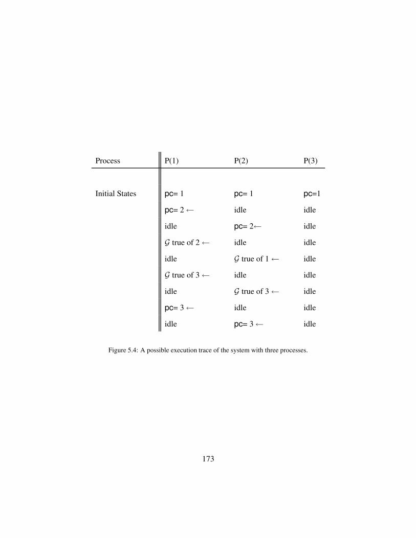
Process P(1) P(2) P(3)

Initial States pc= 1 pc= 1 pc=1

pc= 2← idle idle

idle pc= 2← idle

G true of 2← idle idle

idle G true of 1← idle

G true of 3← idle idle

idle G true of 3← idle

pc= 3← idle idle

idle pc= 3← idle

Figure 5.4: A possible execution trace of the system with three processes.

173

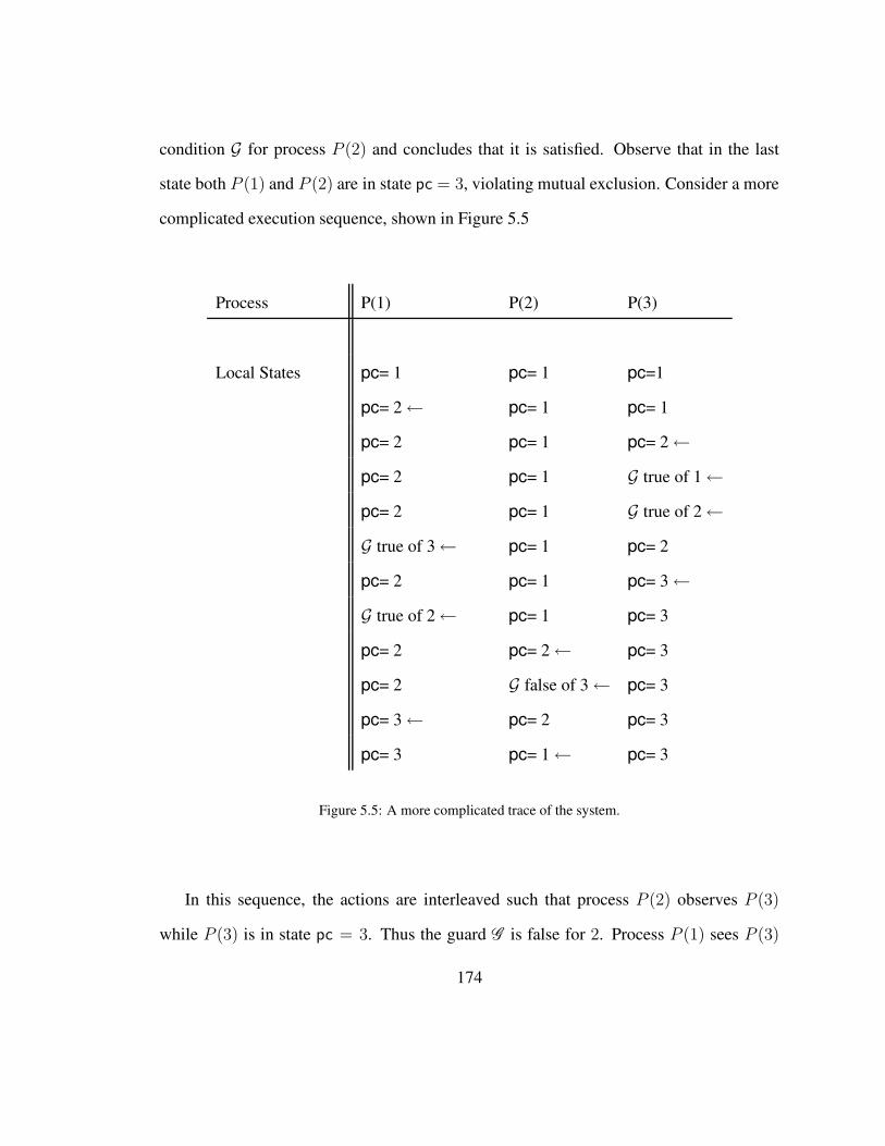
condition G for process P (2) and concludes that it is satisfied. Observe that in the last

state both P (1) and P (2) are in state pc = 3, violating mutual exclusion. Consider a more

complicated execution sequence, shown in Figure 5.5


Local States pc= 1 pc= 1 pc=1

pc= 2← pc= 1 pc= 1

pc= 2 pc= 1 pc= 2←

pc= 2 pc= 1 G true of 1←

pc= 2 pc= 1 G true of 2←

G true of 3← pc= 1 pc= 2

pc= 2 pc= 1 pc= 3←

G true of 2← pc= 1 pc= 3

pc= 2 pc= 2← pc= 3

pc= 2 G false of 3← pc= 3

pc= 3← pc= 2 pc= 3

pc= 3 pc= 1← pc= 3

Figure 5.5: A more complicated trace of the system.

In this sequence, the actions are interleaved such that process P (2) observes P (3)

while P (3) is in state pc = 3. Thus the guard G is false for 2. Process P (1) sees P (3)

174

when it is in pc = 2, thus P (3) does not block P (1). It is clear from these two examples

that the interleaving of actions is crucial and adds considerable complexity to the protocol.

In fact, under the atomicity assumption neither of the traces shown above are legal traces.

In particular, the execution sequences where the observation steps of different processes

are interleaved are excluded by the atomicity assumption. It is precisely because of such

execution sequences that designing a distributed mutual exclusion protocol is challenging.

5.4 Monitors for Handling Non-atomicity

Recall that each process in our system has one pc variable and a collection of data vari-

ables. While it is clear that interleaving of observation steps add considerable complexity

to the protocol, none of the variables used in our systems really tracks the state of these

observations steps. For example, consider again the sample trace shown in Figures 5.4.

Since the observation steps are hidden to the observers on the outside, the execution trace

seen from the outside looks as shown in Figure 5.6.

The current state of process P (i) gives us no information about how much of global

condition it has finished evaluating and how much is still left. For example, at the state

marked idle under column marked P (1) in the figure above, we do not know much of

the guard condition G.= ∀otr 6= slf.pc[otr] 6= 3 has already been evaluated by process

175


Initial States pc= 1 pc= 1 pc=1

pc= 2← idle idle

idle pc= 2← idle

pc= 3← idle idle

idle pc= 3← idle

Figure 5.6: Execution trace seen from the “outside”.

P (1). Thus, if we consider only the visible state of processes, comprising of pc and data

variables, we have no way of knowing the truth or falsity of global conditions 1.

Fortunately, even when the observation steps are invisible, we can gather some in-

formation about the truth or falsity of the guards by looking at the state of each process.

For this, we have to consider the previous states, in addition to the current states, of the

processes. To this end, we will define a collection of monitor processes that track the evo-

lution of the local states of the processes. These monitor processes are non interfering and

are composed synchronously with concrete systems P(K). By synchronously composed

we mean the following: every time a process in P(K) moves, all the monitor processes

run simultanesouly and update their variables based on the current state of the processes

in P(K). Crucially, the construction of the monitor processes is not specific to any par-

ticular protocol. In other words, for any mutual exclusion protocol we can automatically

1Note that, if we assume atomicity, the truth or falsity of guards can be known just by observing the

current states of all processes.

176

construct the monitor processes defined below.

For each process P (i) inP(K) we have a monitor processMg(i). The monitor process

Mg(i) has the following variables

• K − 1 variables mg(i, j), j 6= i one for each process P (j), j 6= i with range

clean, dirty, idle. These monitor variables are used to handle guarded transitions.

• Another set of K−1 variablesmu(i, j), j 6= i one for each process P (j), j 6= i with

range clean, dirty, idle. These variables are used to handle update transitions.

• In addition, there is one variable em[i] with range clean, dirty, idle.

Monitor variables have value idle if they are not in use. Usually, monitor variables

transition to value dirty from value idle. Typically, a monitor variable being dirty indicates

that certain actions are not possible (an exception to this is the value dirty of em variable,

which actually permits more behaviors). After this the monitor variable may transition to

value clean. This value for a monitor variable usually indicates that the monitor variable

has seen enough history information to allow all behaviors. Sometimes a monitor variable

can transition from value idle to clean directly. Once a variable has become clean, it will

stay clean until it is reset to idle.

In the next two subsections we will describe how the monitor variables are updated

by the monitor processes. We will also formalize the exact information that we gain from

monitor processes.

177

Monitor Variables for Guarded Transition

The variable mg(i, j) keeps track of process j and is updated as shown in the Figure 5.7.

The value of mg(i, j) is computed as follows:

1. If process i is not evaluting any guard mg(i, j) = idle.

2. If mg(i, j) = idle and process i is evaluating a guard with condition

G(slf, otr) and G(i, j) is false then mg(i, j) = dirty.

3. If process i is evaluting a guard with condition G(slf, otr) and G(i, j)

is true then mg(i, j) = clean.

4. Otherwise mg(i, j) retains its value

Figure 5.7: Update procedure for monitor variables pertaining to guarded transitions.

Intuitively, the variable mg(i, j) present in monitor Mg(i) tracks whether process j

entered any state that makes the guard condition G(i, j) true while process i is evaluating

the guard G (slf, otr) .= ∀otr 6= slf.G(slf, otr). In such a case, the monitor variable is clean.

Otherwise it is dirty. Informally, the variable mg(i, j) being dirty means that process j will

block the guard G (slf, otr) for process i.

This code is run by the monitor process after each step of the asynchronous system

P(K). Note that, the monitor process does not intefere with the execution of P(K) in any

way.

The variable em(i) with range clean, dirty, idle is updated as shown in Figure 5.8.

178

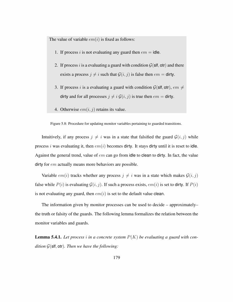
The value of variable em(i) is fixed as follows:

1. If process i is not evaluating any guard then em = idle.

2. If process i is a evaluating a guard with condition G(slf, otr) and there

exists a process j 6= i such that G(i, j) is false then em = dirty.

3. If process i is a evaluating a guard with condition G(slf, otr), em 6=

dirty and for all processes j 6= i G(i, j) is true then em = dirty.

4. Otherwise em(i, j) retains its value.

Figure 5.8: Procedure for updating monitor variables pertaining to guarded transitions.

Intuitively, if any process j 6= i was in a state that falsified the guard G(i, j) while

process i was evaluating it, then em(i) becomes dirty. It stays dirty until it is reset to idle.

Against the general trend, value of em can go from idle to clean to dirty. In fact, the value

dirty for em actually means more behaviors are possible.

Variable em(i) tracks whether any process j 6= i was in a state which makes G(i, j)

false while P (i) is evaluating G(i, j). If such a process exists, em(i) is set to dirty. If P (i)

is not evaluating any guard, then em(i) is set to the default value clean.

The information given by monitor processes can be used to decide – approximately–

the truth or falsity of the guards. The following lemma formalizes the relation between the

monitor variables and guards.

Lemma 5.4.1. Let process i in a concrete system P (K) be evaluating a guard with con-

dition G(slf, otr). Then we have the following:

179

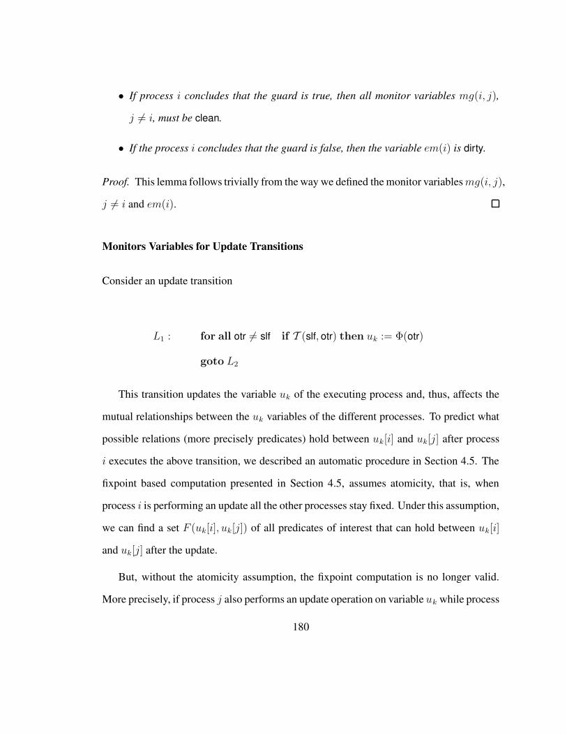
• If process i concludes that the guard is true, then all monitor variables mg(i, j),

j 6= i, must be clean.

• If the process i concludes that the guard is false, then the variable em(i) is dirty.

Proof. This lemma follows trivially from the way we defined the monitor variablesmg(i, j),

j 6= i and em(i).

Monitors Variables for Update Transitions

Consider an update transition


goto L2

This transition updates the variable uk of the executing process and, thus, affects the

mutual relationships between the uk variables of the different processes. To predict what

possible relations (more precisely predicates) hold between uk[i] and uk[j] after process

i executes the above transition, we described an automatic procedure in Section 4.5. The

fixpoint based computation presented in Section 4.5, assumes atomicity, that is, when

process i is performing an update all the other processes stay fixed. Under this assumption,

we can find a set F (uk[i], uk[j]) of all predicates of interest that can hold between uk[i]

and uk[j] after the update.

But, without the atomicity assumption, the fixpoint computation is no longer valid.

More precisely, if process j also performs an update operation on variable uk while process

180

i is doing the same, then we cannot use the fixed point computation to predict which

relationships hold between uk[i] and uk[j] after the update operation. In this case, we

just say that the set of all possible relations between uk[i], uk[j] is simply F(uk[i], uk[j]),

where F(uk[i], uk[j]) is the set of all possible predicates of interest (usually syntactically

picked from the protocol code).

Thus, if we knew that two processes were not updating the same variable t simul-

taneously, then we can better predict the set of possible relations after the update using

the fixpoint computation. The K − 1 variables mu(i, 1), . . . , mu(i, i − 1), mu(i, i +

1), . . . , mu(i, K) with range clean, dirty, idle try to track precisely this information: the

variable mu(i, j) tells us whether process j was updating the same data variable at the

same time as process i. The value of the variable mu(i, j) , j 6= i is computed as shown

in Figure 5.9.

Intuitively, mu(i, j) being clean indicates that, at some point when process i was up-

dating its variable t, process j was also updating the same variable t. We can use the

information contained in the monitor processes to abstract the concrete behaviors as fol-

lows:

• If there is a process j such that mu(i, j) is clean then the valuation of a predicate

involving uk[j] and uk[i] could be anything as uk[j] might have changed while uk[i]

was being updated.

• If process j is such that mu(i, j) is dirty then we know that uk[j] could not have

changed while i was executing the update transition. It is possible to figure out the

possible relationships, after the update, between uk[i] and uk[j] as described above.

181

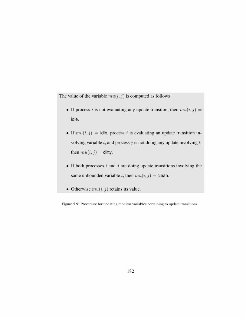
The value of the variable mu(i, j) is computed as follows

• If process i is not evaluating any update transiton, then mu(i, j) =

idle.

• If mu(i, j) = idle, process i is evaluating an update transition in-

volving variable t, and process j is not doing any update involving t,

then mu(i, j) = dirty.

• If both processes i and j are doing update transitions involving the

same unbounded variable t, then mu(i, j) = clean.

• Otherwise mu(i, j) retains its value.

Figure 5.9: Procedure for updating monitor variables pertaining to update transitions.

182

The following lemma formalizes the relationship between the monitor variables and

the update transitions.

Lemma 5.4.2. Suppose process i is updating variable t in an update transition with the

update expression T(slf, otr). Let F (uk[i], uk[j]) be the fixpoint of predicates as computed

in Section 4.5. If mu(i, j) = dirty, then the set of predicates that hold between uk[i] and

uk[j] after process i has finished the update transition is a subset of F (uk[i], uk[j]).

Proof. The proof follows from the fact that mu(i, j) is dirty only if process j was not

updating its uk[j] variable while process iwas updating its uk[i] variable. Thus, by the way

we compute the fixpoint F (uk[i], uk[j]), it contains all the possible relationships between

uk[i] and uk[j] after the update by process i.

Thus, our lack of information about the invisible/hidden steps (used in evaluating

guards and updates) can be overcome by making use of synchronously composed non

interfering monitors and we can build a sound abstraction of the actual behaviors.

Remark 14. Note that a process can either execute a guarded transition or an update tran-

sition, but not both at the same time. Thus, instead of having two sets of variables, namely

mg(i, j), j 6= i and mu(i, j), j 6= i, we can just have one set of variables m(i, j), j 6= i

with range clean, dirty.

From now on, each monitor process Mg(i) will have variables m(i, j)|j 6= i and the

variable em(i).

183

5.4.1 Abstracting the Monitor Variables

As in Chapter 4, we start with descriptions of ∆(x) having the format

pc[x] = i ∧ ±E1(x) ∧ ±E2(x) ∧ · · · ∧ ±ET (x), where i ∈ [1..S].

where the environment prediates Ei(x) are constructed as before. But, the abstract model

constructed using descriptions ∆(x) given above will not have enough detail to verify a

protocol without the atomicity assumption. Therefore, we augment our abstract states so

that, in addition to the state of the reference process and its environment, they also contain

the history information contained in the monitor processes. Our augmented abstract states

will be of the form

〈pc, e1, . . . , eT , t1, . . . , tT , b1, . . . , bT , te〉

where the variables t1, . . . , tT and te (called trackers) abstract the monitor variables

of the reference process, b1, . . . , bT (called backers) abstract the monitor variables of the

environment processes. We now describe how to abstract the different monitor variables.

Abstracting Trackers

Consider first the reference process x. Apart from the reference process, no other process

is individually identifiable in the abstract state. Corresponding to each environment condi-

tion Ei, we have an abstract variable ti with range clean, dirty, both which abstracts the

information present in the monitors. The value of ti is computed as follows:

184

• If for all the processes y satisfying environment predicate Ei(x, y) the variable

m(x, y) = clean, then ti = clean.

• If for all the processes y satisfying environment predicate Ei(x, y) the variable

m(x, y) = dirty, then ti = dirty.

• Otherwise ti = both.

Given a concrete state s of a systemP(K) with reference process x and an environment

Ei, the value of tracker ti is uniquely determined. We denote the function from (s, x, i) to

ti by F t. This function will be used later on.

In addition, we have another variable te that abstracts the monitor variable em(x). The

value of te is exactly the same as value of em(x).

Abstracting Backers

Trackers maintain history information that is relevant for the reference process. We also

need to abstract the information present in the monitors for processes other than the ref-

erence process x. In particular, for each environment process y, we are interested in the

monitor variable m(y, x). As noted earlier, environment processes are grouped according

to the environment condition they satisfy. For an environment Ei, we maintain a variable

bci that combines the m(y, x) variables of all processes y in the environment Ei. The value

of bci is computed as follows:

• If for all processes y satisfyingEi(x, y) we have m(y, x) = clean, then bci = clean.

185

• If for all processes y satisfying Ei(x, y) we have m(y, x) = dirty, then bci = dirty.

• Otherwise bci = both.

Given a concrete state s of a systemP(K) with reference process x and an environment

Ei, the value of bci is uniquely determined. We can denote the function from (s, x, i) to bci

by F b. This function will be used later on.

We will now define the abstraction mapping from augmented concrete states to aug-

mented abstract states.

Definition 5.4.3 (Abstraction Mapping). Let P (K), K > 1, be a concrete system and

p ∈ [1..K] be a process. The abstraction mapping αp induced by p maps a global state s

of P(K) to an abstract state 〈pc, e1, . . . , eT , t1, . . . , tT , b1, . . . , bT , te〉 where

• pc = the value of pc[p] in state s and for all ej, we have ej = 1⇔ s |= Ej(p).

• For all j we have tj = F t(s, p, j), and for all j, we have bj = F b(s, p, j)

The corresponding augmented abstract model PA is defined as in Section 2.5.2. The

set of labels is the same as the labels used in Section 4.2. From the coverage and congru-

ence properties of the original abstract descriptions we can conclude that the same prop-

erties hold for the augmented abstract descriptions as well. Thus, the following corollary

follows from Theorem 2.2.4.

Corollary 5 (Soundness of Augmented Abstraction). Let P(N) be a parameterized

mutual exclusion system, PM(N) be an augmentation of P(N) with monitor processes

186

as described above, and PMA be its augmented abstraction. For an indexed property

∀x.Φ(x), where Φ(x) is a control condition we have

PMA |= Φ(x)⇒ ∀K.PM(K) |= ∀x.Φ(x)⇒ ∀K.P(K) |= ∀x.Φ(x)


As in the atomicity case, we consider the following four cases for computing an over-

approximation of a transition statement:

Active process is . . . guarded transition update transition

. . . reference process Case 1 Case 2

. . . environment process Case 3 Case 4

Before we begin, we recall the notation introduced earlier in Section 4.5. The envi-

ronment condition Ei(x, y).= y 6= x ∧ Rj(x, y) ∧ pc[y] = L is denoted by E(j,L)(x, y).

The corresponding environment predicate is referred to as E(j,L)(x) and the corresponding

abstract variable is e(j,L). The set of all environment conditions E(j,L)(x, y) is referred to

as EL.

5.5.1 Case 1: Guarded Transition for Reference Process

Let us now turn to Case 1 and consider the guarded transition tG:


187

Suppose at least one of the trackers ti, i ∈ [1..T ] is not clean. Then the reference

process cannot conclude the guard is true. If all the trackers are clean, then we may

conclude that the guard is true or false. Once reference process x ends up in a new control

location, we have to appropriately assign new values to the trackers and the backers. To

do this we need the following two definitions. The first definition is exactly the same as

the one in Chapter 4, but we repeat it for the sake of completeness.

Definition 5.5.1 (Blocking Set for Reference Process). Let G.= ∀otr 6= slf.G(slf, otr) be

a guard. We say that an environment condition Ei(x , y) blocks the guard G if Ei(x , y)⇒

¬G(x , y). The set Bx(G ) of all indices i such that Ei(x , y) blocks G is called the blocking

set of the reference process for guard G .

Note that either Ei(x , y) ⇒ ¬G(x , y) or Ei(x , y) ⇒ G(x , y) holds for every environ-

ment Ei(x , y).

Each environment Ei uniquely determines the control location of the processes satis-

fying it. We will assume, for simplicity, that there is only one transition starting at each

control location 2. Thus, each environment Ei has an unique guard or update expression as-

sociated with it. The following notion of dependent environments for guarded transitions

is similar to the blocking set for the reference process.

Definition 5.5.2 (Dependent Set for Guards). Let pc = L be a control location of the

reference process. The guard dependent set of L, Dg(L) contains all those environments

whose associated guard G.= ∀otr 6= slf.G(slf, otr) are such that Ei(y, x) ∧ G(y, x) ∧

(pc[x] = L) is satisfiable.

2Extension to the general case is simple.

188

Intuitively, the guard dependent set of a control location pc = L is the set of all those

environments whose associated guards are such that the reference process x in control

location pc = L does not contradict the guards. Thus, a process y present in any such

environment could have seen the reference process x satisfy process y’s guard. We define

update dependent sets similarly.

Definition 5.5.3 (Dependent Set for Updates). Let pc = L be a control location of the

reference process. The update dependent set of L, Du(L), contains those environments

whose associated update expression updates the same data variable as the update transition

associated with L. If there is no update transition associated with pc = L then the set is

empty.

We will now explain how to abstract the guarded transition tG

L1 : if ∀otr 6= slf.G(slf, otr) then goto L2 else goto L3.

We will represent the set of abstract transition arising from this case by an invariant (be-

tween current and next states) IxtG . The invariant, structured similar to the one in Sec-

tion 4.5, will be presented in terms of three conditions GR1, GR2, GR3. The abstract

model will have transition from s1 = 〈pc, e1, .., eT , t1. . . . , tT , bc1, . . . , bcT , te〉 to

s2 = 〈pc′, e1, .., eT , t′1. . . . , t

′T , bc

′1, . . . , bc

′T , te

′〉 if

GR1. pc = L1, i.e., the reference process is in location L1,

GR2. One of the following two conditions holds:

189

• Then Branch: ∀i).(ti = clean) and pc′ = L2, i.e., the guard is true and the

reference process moves to control state L2.

• Else Branch: ¬(∀i.ti = clean) ∨ (∀i.ti = clean ∧ te = dirty) and pc′ = L3,

i.e., the guard is false and the reference process moves to control state L3. Note

that the condition te = dirty indicates that at least one tracker was dirty at some

point in the past.

GR3 Assuming pc′ = L where L ∈ L2, L3 the following conditions hold.

• If the transition associated with control location L is a guarded transition with

G.= ∀otr 6= slf.G (slf, otr), then the following conditions hold.

– If i ∈ Bx(G) or e′i = 0 then t′i = clean. Else t′i = dirty, i.e., if Ei is a not

blocking environment or if the environment is empty the corresponding

tracker is clean. Otherwise, it is set to dirty as there is a process in a

blocking environment.

– If i ∈ Dg(L) ∪ Du(L), then bc′i = clean else bc′i = bci. i.e., if the

reference process does not block the guard associated with environment

Ei or updates the same variable as the update transition associated with Ei

then bci is set to clean, otherwise it is set to dirty.

– If there exists an i such that t′i = dirty then te = dirty, i.e., the variable te

is dirty if at least one of the trackers is dirty.

• If the transition associated with control location L is an update transition then

the following conditions hold

190

– If i ∈ Du(L) and e′i = 1 then t′i = clean. Else t′i = dirty. That is, if

environment ei updates the same data variable as the reference process in

control location L, then the tracker ti must be set to clean otherwise ti is

set to dirty. This indicates that both the reference process and a process in

ei can change the same data variables simultaneously.

– If i ∈ Dg(L), then bc′i = clean else bc′i = bci. That is, if control location

L is such that the guard associated with ei is not blocked by the reference

process in control location L, then the backer bci is set to clean.

– te′ = clean. This is a default value for te as it is not really used for update

transitions.

Similar to the concrete monitor variables, the value clean for trackers and backers is

the most permissive –that is, if backers and trackers are clean, then the possible set of

transitions is maximal. The value both is slightly more restrictive than clean: the envi-

ronments corresponding to trackers and backers that are in the both state cannot be empty.

The value dirty is the most restrictive. A tracker being dirty prevents the reference pro-

cess from moving forward. Similarly, a backer being dirty prevents the processes of the

corresponding environment from moving forward.

Lemma 5.5.4. If states s1 and s2 in a concrete system P(K), K > 1 are such that

αc(s1) = s1 and αc(s2) = s2 and there is a transition from s1 to s2 via process c exe-

cuting a guarded transition tG then s1 and s2 satisfy the transition invariant IxtG .

Proof. This follows simply from the way we constructed the invariant.

191

Note that all we have done is to translate the lemmas listed in Section 5.4 in terms

of the reference process and its environment. This is precisely where the power of this

approach comes from. Constructing the abstract model is theoretically simple and it is

easily extendible in case new constructs are allowed in the concrete protocols.

5.5.2 Case 2: Guarded Transition for Environment Processes

Suppose that the guarded transition tG


is executed by a concrete process y satisfying the environment condition E(i,L1)(x, y).

The active process thus switches from environment condition E(i,L1)(x, y) to environment

condition E(i,L2)(x, y) or E(i,L3)(x, y). Note that in a guarded transition, only the pc of the

active process changes.

We denote the abstract transition corresponding to this case by an invariant I yi (tG). We

introduce an abstract transition from s1 = 〈pc, e1, .., eT , t1. . . . , tT , bc1, . . . , bcT , te〉 to

s2 = 〈pc′, e′1, .., e′T , t

′1. . . . , t

′T , bc

′1, . . . , bc

′T , te〉 if the following conditions hold. For

brevity we will represent the environment condition E(i,L1) by E1, E(i,L2) by E2, E(i,L3)

by E3.

GE1. e1 = 1, that is, there is an environment process in state control location L13.

3The requirement that, for each control location L, there be only one transition starting from L is being

192

GE2 One of the following two conditions holds:

• Then Branch: bck ∈ clean, both and e′2 = 1, i.e., the guard is true and the

reference process moves to control state L2. e′1 can be 0 or 1.

• Else Branch: e′3 = 1, i.e., the guard is false and the environment process moves

to control state L3. e′1 can be 0 or 1.

GE3. pc′ = pc. That is, the control location of the reference does not change.

GE4. Let the new control location of the environment process be L ∈ L2, L3. Denote

the environment E(i,L) by Ej for the sake of brevity. The following conditions must

hold:

• t′j = ω(t1, tj). Function ω, described below, takes the current values of the

trackers t1, tj and returns the new value for tj .

• t′1 = Ωt(t1, e′1). Function Ωt, described below, takes the current value of a

tracker (or a backer) and the next state value of the corresponding environment

and returns the next state value of the tracker (or the backer).

• bc′1 = Ωt(bc1, e′1).

• If the transition associated with L is a guarded transition then

bc′j = Ωb(Dg(L), bcj). Function Ωb finds the new value of backer bcj as a

function of the current value of the backer bcj and the guard dependent set of

control location L.

used here.

193

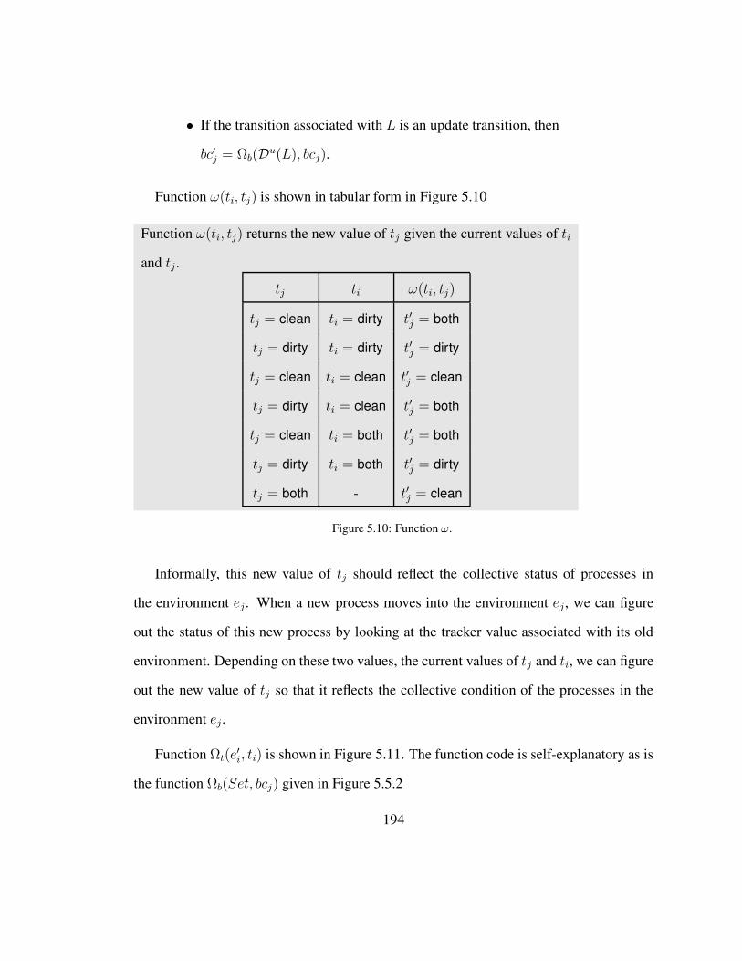
• If the transition associated with L is an update transition, then

bc′j = Ωb(Du(L), bcj).

Function ω(ti, tj) is shown in tabular form in Figure 5.10

Function ω(ti, tj) returns the new value of tj given the current values of ti

and tj.

tj ti ω(ti, tj)

tj = clean ti = dirty t′j = both

tj = dirty ti = dirty t′j = dirty

tj = clean ti = clean t′j = clean

tj = dirty ti = clean t′j = both

tj = clean ti = both t′j = both

tj = dirty ti = both t′j = dirty

tj = both - t′j = clean

Figure 5.10: Function ω.

Informally, this new value of tj should reflect the collective status of processes in

the environment ej . When a new process moves into the environment ej, we can figure

out the status of this new process by looking at the tracker value associated with its old

environment. Depending on these two values, the current values of tj and ti, we can figure

out the new value of tj so that it reflects the collective condition of the processes in the

environment ej.

Function Ωt(e′i, ti) is shown in Figure 5.11. The function code is self-explanatory as is

the function Ωb(Set, bcj) given in Figure 5.5.2

194

Function Ωt(e′i, ti) returns the new value of the tracker ti given the current

value of the tracker and the next value of the corresponding environment

bit ei.

• If e′i = 0 then t′i = clean

• Otherwise

– If ti = clean then t′i = clean

– If ti = dirty then t′i = dirty

– If ti = both then t′i ∈ clean, dirty, both

Figure 5.11: Function Ωt.

Lemma 5.5.5. If states s1 and s2 in a concrete system P(K), K > 1 are such that

αc(s1) = s1 and αc(s2) = s2, c ∈ [1..K] and there is a transition from s1 to s2 via

process d 6= c executing a guarded transition tG, then s1 and s2 satisfy the transition

invariant Iy(tG).

Proof. The proof of this lemma follows directly from the way we constructed Iy(tG).

5.5.3 Case 3: Update Transition for Reference Process

Consider the case where the reference process is executing an update transition tU :

195

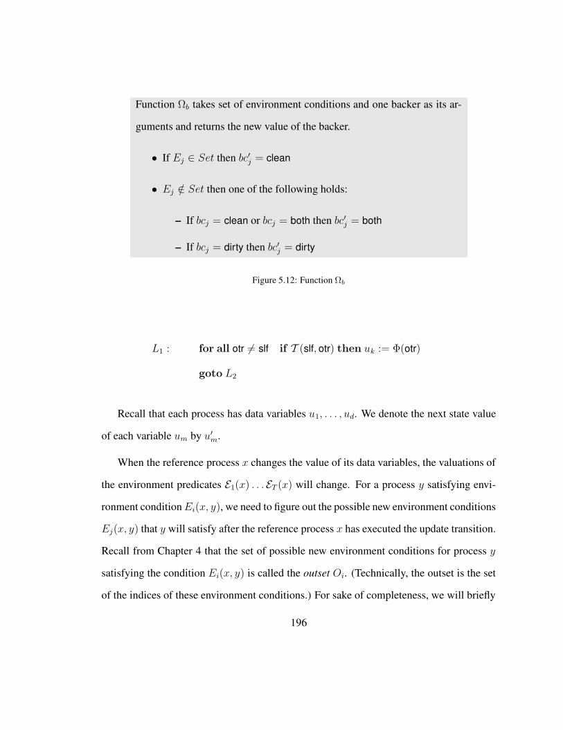
Function Ωb takes set of environment conditions and one backer as its ar-

guments and returns the new value of the backer.

• If Ej ∈ Set then bc′j = clean

• Ej /∈ Set then one of the following holds:

– If bcj = clean or bcj = both then bc′j = both

– If bcj = dirty then bc′j = dirty

Figure 5.12: Function Ωb


goto L2

Recall that each process has data variables u1, . . . , ud. We denote the next state value

of each variable um by u′m.

When the reference process x changes the value of its data variables, the valuations of

the environment predicates E1(x) . . . ET (x) will change. For a process y satisfying envi-

ronment conditionEi(x, y), we need to figure out the possible new environment conditions

Ej(x, y) that y will satisfy after the reference process x has executed the update transition.

Recall from Chapter 4 that the set of possible new environment conditions for process y

satisfying the condition Ei(x, y) is called the outset Oi. (Technically, the outset is the set

of the indices of these environment conditions.) For sake of completeness, we will briefly

196

explain again how to compute the outset.

Case A.

The first case we need to consider is when process y does not update uk while the reference

process is updating its variable. Denote by T(x, y) the update formula T (x, y) ∧ u′k[x] :=

φ(y) ∨ ¬T (x, y) ∧ u′k[x] := uk[x]. Given the update formula, we find what possible

inter-predicates involving u′k[x], uk[y] can be true. Formally, the set C1(uk) of these inter-

predicates is given by all formulas uk[x] ≺ uk[y] where ≺∈ <,>,= such that

u′k[x] ≺ uk[y] ∧ T(x, y) is satisfiable.

The possible relationships between uk[x] and uk[y] might change when x repeatedly up-

dates its uk value by looking at other processes. Suppose x looks at another process z and

updates its uk[x] value again. We now find the set C2(uk) of possible relationships be-

tween uk[x] and uk[y] after the new update involving process z under the assumption that

a relation from C1(uk) holds before the update. Thus, the new set C2(uk) of relationships

is given by all formulas uk[x] ≺ uk[y] where ≺∈ <,>,= such that

u′k[x] ≺ uk[y] ∧ T(x, z) ∧ ψ(x, y) is satisfiable and ψ(x, y) ∈ C1(uk).

Note that C1(uk) ⊆ C2(uk) because the definition of T(x, z) allows the possibility that

the value of uk[x] remains unchanged. We similarly compute sets C3(uk), C4(uk) . . . until

a fixpoint, C(uk), is reached.

In the environment condition Ei(x, y), let θ be the (unique) inter-predicate that de-

scribes the relation between uk[x] and uk[y]. Consider the set of environment conditions

197

Ej(x, y) that are obtained from Ei(x, y) by replacing θ with a formula in the fixpoint

C(uk): the indices of these environment conditions constitute the outset Oi of Ei(x, y).

Correspondingly, the inset Ik ⊆ 1..T for environment conditionEk(x, y) consists of

all j such that k ∈ Oj.

Case B.

In the second case, process y is also updating its uk variable. In this case, the set C(uk)

is the set of all possible predicates involving uk[x] and uk[y]. In other words, we cannot

predict what the relationship between uk[x] and uk[y] is. The outset consisting of [the

indices of] environments is then computed as described.

In the abstract model, to compute the outset for environment em we use Case A if

the associated tracker tm is dirty; otherwise we use Case B. Observe that, if the tracker is

clean, more behaviors are possible.

Denote the set of abstract transitions corresponding to the concrete update transition

(†) by Ix(tU). Ix(tU) has a transition from s1 = 〈pc, e1, .., eT , t1. . . . , tT , bc1, . . . , bcT , te〉

to s2 = 〈pc′, e′1, .., e′T , t

′1. . . . , t

′T , bc

′1, . . . , bc

′T , te〉 if the following conditions hold:

UR1. pc = L1, i.e., the reference process first is in control location L1.

UR2. pc′ = L2, i.e., the reference process moves to control location L2.

UR3. ∀k ∈ [1..T ].(ek = 1 ⇒ ∃j ∈ Ok.e′j = 1), i.e., if there was a process in environ-

ment Ek(x) before the transition, then there must be a process in one of the outset

environments Ok of Ek(x, y) after the transition.

198

UR4. ∀j ∈ Ik.(ej = 0 ⇒ e′k = 0), i.e., if there is no process satisfying the inset environ-

ments Ik of environment Ek(x, y) before the transition then after the transition there

can be no process in environment Ek(x, y).

UR5. for each k ∈ [1..T ], the value of bc′k is computed as follows

• if e′k = 0 or k ∈ Dg(L2) ∪ Du(L2) then bc′k = clean

• otherwise we have three cases:

– if ∀j ∈ Ik.bcj = clean then bc′k = clean

– if ∀j ∈ Ik.bcj = dirty then bc′k = dirty

– if ∃j ∈ Ik.bcj = clean and ∃j ∈ Ik.bcj = dirty then bc′k can take any value

in clean, dirty, both

UR6. For each k ∈ [1..T ] if k ∈ D(()L2) then t′k = clean else t′k = dirty where D(L2) is

either Bx(G), if the transition associated with L2 is a guarded transition with guard

condition G, or D(L2) is Du(L2), if the transition associated with L2 is an update

transition.

Lemma 5.5.6. If states s1 and s2 in a concrete system P(K), K > 1, are such that

αc(s1) = s1 and αc(s2) = s2, with c ∈ [1..K] and there is a transition from s1 to s2

via process c executing a guarded transition tU then s1 and s2 satisfy Ix(tG).

Proof. The proof of this lemma follows directly from the way we constructed Ix(tG).

199

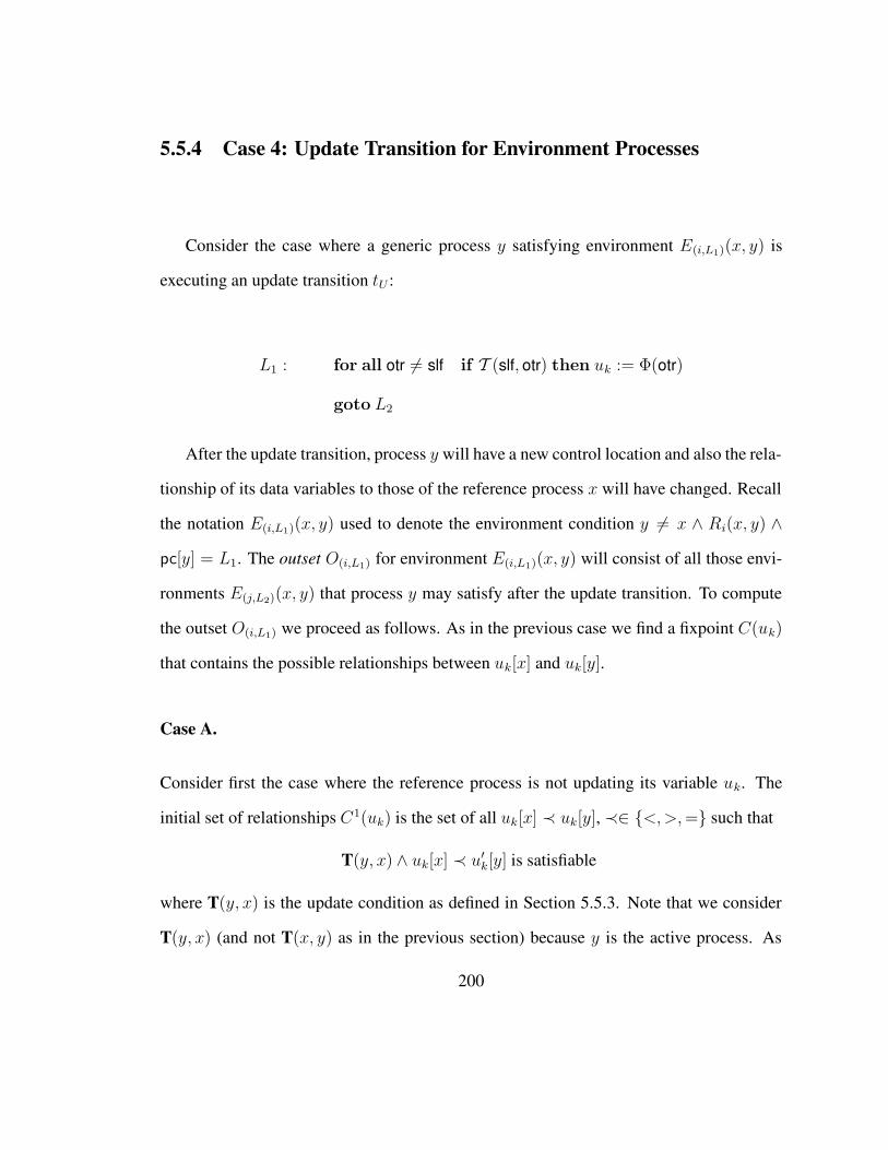
5.5.4 Case 4: Update Transition for Environment Processes

Consider the case where a generic process y satisfying environment E(i,L1)(x, y) is

executing an update transition tU :


goto L2

After the update transition, process y will have a new control location and also the rela-

tionship of its data variables to those of the reference process x will have changed. Recall

the notation E(i,L1)(x, y) used to denote the environment condition y 6= x ∧ Ri(x, y) ∧

pc[y] = L1. The outset O(i,L1) for environment E(i,L1)(x, y) will consist of all those envi-

ronments E(j,L2)(x, y) that process y may satisfy after the update transition. To compute

the outset O(i,L1) we proceed as follows. As in the previous case we find a fixpoint C(uk)

that contains the possible relationships between uk[x] and uk[y].

Case A.

Consider first the case where the reference process is not updating its variable uk. The

initial set of relationships C1(uk) is the set of all uk[x] ≺ uk[y], ≺∈ <,>,= such that

T(y, x) ∧ uk[x] ≺ u′k[y] is satisfiable

where T(y, x) is the update condition as defined in Section 5.5.3. Note that we consider

T(y, x) (and not T(x, y) as in the previous section) because y is the active process. As

200

y updates its uk variable repeatedly, the relationship between uk[x], and uk[y] will also

change. To compute all the possible relationships, we use an approach similar to the

fixpoint computation in Case 3. Thus, we find the set C2(uk) of all uk[x] ≺ uk[y], ≺∈ <

,>,=, such that

T(y, z) ∧ uk[x] ≺ u′k[y] ∧ ψ(x, y) is satisfiable

where ψ(x, y) ∈ C1(uk). We similarly compute C3(uk), C4(uk), . . . until we reach a

fixpoint C(uk).

Case B.

Consider now the case where the reference process is also updating its uk variable. In this

case, C(uk) will consist of all possible relations on uk[x] and uk[y], denoting that we do

not have enough information.

In the environment condition E(i,L1)(x, y), let θ be the (unique) inter-predicate that

describes the relation between uk[x] and uk[y]. Consider the set of environment conditions

E(j,L2)(x, y) that are obtained fromE(i,L1)(x, y) by replacing θ by a formula in the fixpoint

C(uk) and replacing the condition pc[y] = L1 by pc[y] = L2. The indices of these

environment conditions constitute the outset O(i,L1) of E(i,L1)(x, y).

To compute the outset for an environment e(i,L1), we will use Case A if the associated

backer bc(i,L1) is dirty. Otherwise, we use Case B. Note again that bc(i,L1) being clean or

both allows more behaviors.

Since the transition starts at control location L1 and a generic process executes it, we

will describe the abstract transition I i,ky (tU) for each environment condition E(i,L1)(x, y)

201

and each k ∈ O(i,L1). The abstract transition Iy(tU) for Case 4 will be

∨

E(i,L1)(x,y)

∨

k∈O(i,L1)

I i,ky (tU).

I i,ky (tU ) has a transition from s1 = 〈pc, e1, .., eT , t1. . . . , tT , bc1, . . . , bcT , te〉 to s2 =

〈pc′, e′1, .., e′T , t

′1. . . . , t

′T , bc

′1, . . . , bc

′T , te〉 if the following conditions hold. For brevity we

will represent the environment condition E(i,L1) by E1 and E(j,L2) by E2.

UR1. pc = pc′, i.e., the reference process does not move.

UR2. e1 = 1, i.e., there is a process in environment E(i,L1)(x,y) before the transition.

UR3. e′2 = 1, i.e., there is a process in environment E(j,L2)(x,y) after the transition.

UR4. The e variables except e′1, e′2 do not change, i.e., e′l = el for l /∈ (i, L1), (j, L2).

UR5. Assuming the new control location of the environment process that moved was

L ∈ L2, L3, denote the environment E(i,L) by Ej . The following conditions must

hold:

• t′2 = ω(t1, t2)

• t′1 = Ωt(e1, t1)

• bc′1 = Ωt(e1, bc1)

• If the transition associated withL is a guarded transition bc′j = Ωb(Dg(L), bci, bcj).

• If the transition associated withL is an update transition bc′j = Ωb(Du(L), bci, bcj).

202

Inter-preds Intra-preds Reachable states Safety

Bakery (NA) 3 5 O(2400) 3800s

Bakery (A) 3 5 O(2146) 68.55s

Figure 5.13: Running Times for the bakery protocol. Bakery(A) and Bakery(NA) stand for the bakery

protocol with and without the atomicity assumption

Lemma 5.5.7. If states s1 and s2 in a concrete system P(K), K > 1, are such that

αc(s1) = s1 and αc(s2) = s2, with c ∈ [1..K] and there is a transition from s1 to s2 via

process d 6= c, executing a guarded transition tU then s1 and s2 satisfy Iy(tU).

Proof. The proof of this lemma follows directly from the way we constructed Iy(tU).

5.6 Experimental Results

We applied our abstraction method to the Bakery and Szymanski’s protocols without

the atomicity assumption. We were able to verify the safety property of the Bakery proto-

col, namely

∀x.∀y 6= x.AG(pc[x] = crit⇒ pc[y] 6= crit)

in about 2 hours. The following table shows the run times and other statistics in the non-

atomic case and the same verification carried out under the atomicity assumption

Note the enormous increase in the state space size once we remove the atomicity as-

sumption. The increase in the model checking is equally dramatic. This again underlines

203

the significant reduction in complexity of protocols due to the atomicity assumption.

We were not able to verify the safety property of Szymanski’s protocol. The correct-

ness of Szymanski’s protocol depends on the specific order in which a process looks at the

other processes in the system. Szymanski’s protocol is correct only if a process looks at the

other processes in the increasing order of the index [55; 77]. The semantics we assigned

to our guarded and update transitions was such that the order of processes was immaterial.

Hence we cannot accurately model Szymanski’s protocol in our input language.

We also applied our abstraction to the toy protocol described in Section 5.3. As ex-

pected, our method finds a trace violating the mutual exclusion protocol in under 5 mins.

204

Chapter 6

Verification by Network Decomposition

6.1 Introduction

Despite the big success of model checking in hardware and software verification, the clas-

sical approach to model checking can handle only finite state systems. Consequently, ap-

plying model checking techniques to systems involving unlimited concurrency, unlimited

memory, or unlimited domain sizes, is a major challenge. Researchers have sought to ad-

dress these issues by different verification methods including, among others, abstraction,

regular model checking, static analysis, and theorem proving.

Many software and hardware systems, however, are described in terms of natural pa-

rameters and, for each concrete value of the parameters, the systems have a finite state

205

space. Verifying a property of a parameterized system amounts to verifying this prop-

erty for all values of the parameters. Examples of parameterized systems include mutual

exclusion protocols, cache coherence protocols, and multi-threaded systems.

While there has been considerable effort in verifying parameterized systems such as

cache protocols and mutual exclusions, that have replicated but no underlying network

graphs, there is little work on parameterized systems that have replicated process and

underlying network graphs. Common examples of systems that are required to operate on

arbitrary network topologies are network routing protocols. Leader election protocols, for

example, are usually designed to operate no matter what the underlying network topology

of the system. Verifying such systems is obviously complicated by the fact that the network

graph can be arbitrary (in addition to the fact the network graph induces asymmetry in the

system).

In a seminal paper, Emerson and Namjoshi [37] consider systems composed of iden-

tical asynchronous processes which are arranged in a ring topology and communicate by

passing a Boolean token. For several classes of indexed CTL∗ \ X properties [15] they

provide cutoffs, i.e., reductions to single systems of constant small size. Consequently,

CTL∗ \ X properties over an infinite class of networks can be reduced to a single model

checking call.

In this chapter, we extend the results of Emerson and Namjoshi from rings to arbitrary

classes of networks. There are two modifications, however: first, our results hold true

only for LTL\X , and second, we introduce a more refined notion of cut-offs. The first

restriction is necessary: We show in Section 4 that with CTL\X it is impossible to obtain

206

cut-offs for arbitrary networks.

The second modification actually provides an interesting new view on the notion of cut-

offs: in order to verify the parametrized system, we are allowed to model check a constant

number c of small systems whose network graphs have sizes bounded by a constant s.

Then, the verification result for the parametrized system is a Boolean combination of the

collected results for the small systems. We call such a reduction to a finite case distinction

a (c, s)-bounded reduction.

Our main results can be summarized as follows:

• Verification by Network Decomposition: Verifying systems with fixed large net-

work graphs G (e.g., concrete instantiations of a parametrized system) can be as

challenging as verifying parameterized systems. Note that when |Q| is the state

space of the individual processes, then the state space of the whole network can be

as high as |Q|n, where n is the number of nodes. We show that the verification of

an indexed LTL\X property ϕ for a system with network graph G can be achieved

by an efficiently computable (c, s)-bounded reduction. For the important case of

2-indexed properties, it is sufficient to model check at most 36 networks of size 4.

• Offline Verification: In a scenario where ϕ is known in advance and the network G

can change for different applications, we can first verify a constant number of small

systems offline. Later, when we get to know the network graph G, the correctness

of G with respect to specification ϕ can be verified online by simply evaluating a

constant size Boolean function, regardless of the size of the processes.

207

Again, for 2-indexed properties, the offline computation involves at most 36 calls to

the model checker for networks of size 4.

• Cut-Offs: For every class of networks T and k-indexed LTL\X property ϕ one can

verify if ϕ holds on all networks in T by a (c, s)-bounded reduction, where c and s

depend only on k.

Depending on the complexity of the networks in T, finding a suitable (c, s)-bounded

reduction will in general still involve manual algorithm design. Similar to famous

results about linear time algorithms for bounded tree-width [25], our proofs just

guarantee the existence of small reductions.

Our results lay the foundation for reasoning about systems with arbitrary network

graphs. While communication between the processes is simple, the results we obtain are

non-trivial. In fact, we were surprised to discover that for CTL \X specification there are

no cutoffs even for the simple communication model. The generalized notion of cutoffs we

present will be crucial to reasoning about systems with more complicated communication.

This chapter is organized as follows: the next section contains the work closest to our

work. In Section 3, we describe the system model in detail. Section 4 contains the main

cutoff results. Section 5 shows that no cutoffs exist for CTL \X . Finally, the conclusion

in Section 5 briefly considers further performance enhancements for practical applications

of our method.

208

6.2 Related Work.

Verification of parameterized systems is well known to be undecidable [2; 76]. Many

interesting approaches to this problem have been developed over the years, including the

use of symbolic automata-based techniques [1; 10; 12; 13; 51; 78], network invariants

[3; 64], predicate abstraction [52; 53], and symmetry reduction [24; 31; 38; 39; 40]. In

[11], cut-offs were used for the verification of systems sharing common resources, where

the access to the resources is managed according to a FIFO-based policy.

In addition to [37] mentioned above, Emerson et al. have shown a large number of fun-

damental results involving cut-offs. The paper [33] by Emerson and Kahlon also considers

LTL\X cut-offs for arbitrary network topologies with multiple tokens, but each token is

confined to two processes which renders their model incomparable to ours. Other previ-

ous work by Emerson and Kahlon [32; 34; 35] consider other restricted forms of process

interaction. Finally, [43] considers the verification of single index properties for systems

with multiple synchronous processes.

Indexed temporal logic was introduced in [15]. The paper also considers identical

processes arranged in ring topology.

The work that is closest in spirit to our negative results on CTL∗ \X logic is the work

by Browne, Clarke and Grumberg in [14] that shows how to characterize Kripke structures

up to bisimilarity using fragments of CTL?. Our results show that even CTL∗ \ X with

only two atomic propositions is sufficient to describe an infinite class of Kripke structures

that are not bisimilar to each other. In other words, bisimilarity over the class of Kripke

structures with two labels gives rise to an infinite number of equivalence classes.

209

6.3 Computation Model

Network Topologies. A network graph is a finite directed graph G = (S,C) without

self-loops, where S is the set of sites, and C is the set of connections. Without loss of

generality we assume that the sites are numbers, i.e., S = 1, 2, . . . , |S|. A (network)

topology T is a class of network graphs.

Token Passing Process. A single token passing process P (process) is a labeled transition

system (Q,Σ, δ, I) such that:

• Q = Q × B, where Q is a finite, nonempty set and B = 0, 1. Elements of Q

will be called local states. The boolean component of a local state indicates the

possession of the token. We say that a local state (q, b) holds the token if b = 1.

• Σ = Σf ∪Σd∪rcv, snd is the set of actions. The actions in Σd are token dependent

actions, those of Σf are called token independent actions, and rcv, snd are actions

to receive and send the token. The sets Σf , Σd are mutually exclusive.

• δ ⊆ Q×Σ×Q is a transition relation, such that every ((q, b), a, (q ′, b′)) ∈ δ fulfills

the following conditions:

(a) A free transition does not change token possession: a ∈ Σf ⇒ b = b′

(b) A dependent transition can execute only if the process possesses the token:

a ∈ Σd ⇒ b = b′ = 1

(c) A receive establishes possession of token: a = rcv⇒ b = 0, b′ = 1

(d) A send revokes the possession of token: a = snd⇒ b = 1, b′ = 0

210

• I ⊆ Q is the set of initial states.

Topological Composition. Let G = (S,C) be a network graph and P = (Q,Σ, δ, I)

be a single token process. Then PG denotes the concurrent system containing n = |S|

instances of P denoted by Ps, s ∈ S. The only synchronization mechanism between the

processes is the passage of a token according to the network graphG. Formally, the system

PG is associated with a transition system (Q,∆, I) defined as follows:

• Q = (q1, . . . , qn) ∈ Qn | exactly one of the qi holds the token.

• ∆ ⊆ Q2n is defined as follows: a transition (q1, q2, . . . , qn) → (q′1, q′2, . . . , q

′n) is in

∆ in one of two cases:

(a) Asynchronous Transition: there exist an index j ∈ 1, . . . , n and an action

a ∈ Σf ∪Σd such that (qj, a, q′j) ∈ δ, and for all indices i 6= j we have qi = q′i.

In other words, only process Pj makes a transition (different from a send or

receive).

(b) Token Transition: there exist a network connection (j, k) ∈ C in the network

graph, such that (qj, snd, q′j) ∈ δ, (qk, rcv, q′k) ∈ δ, and qi = q′i for all indices i

different from j, k.

• I = (q1, . . . , qn) ∈ In | exactly one of the qi holds the token.

An execution path is considered fair if and only if every process Pi receives and sends the

token infinitely often. We assume that every system PG that we consider has fair paths. An

211

immediate consequence of the fairness condition is that a system P G can have fair paths

only if G is strongly connected.

We shall use indexed temporal logics, which can refer explicitly to the atomic propo-

sitions of each process Pi, to specify properties of the compound systems. For each local

state q in Q we introduce propositional variables q(1), . . . , q(n). The atomic proposition

q(i) says that process Pi is in state q. Thus, for a global state g we define

g |= q(i) iff in global state g, process Pi is in state q.

Starting from this definition for atomic propositions, we can easily define common tempo-

ral logics such as CTL or LTL in a canonical way. Throughout this paper, we will assume

that the path quantifiers A and E quantify over fair paths. Further we assume that LTL

formulas are implicitly quantified by E. This restriction simplifies our proofs but does not

restrict generality.

Example 6.3.1. The formula G(q(1)⇒ Fq(2)) says that whenever process P1 is in state

q then process P2 will be in state q sometime in the future.

For increased expressibility we permit that in an atomic formula q(x) the process index

x is a variable (called index variable) which can take any value from 1 to |S|, the total num-

ber of processes. Thus, x can refer to arbitrary processes. We shall write ϕ(x1, . . . , xn)

to indicate that the temporal formula ϕ depends on the index variables x1, . . . xn. We can

substitute the index variables in a formula ϕ(x1, . . . , xk) by integer values i1, . . . , ik in the

natural way, and denote the resulting formula by ϕ(i1, . . . , ik).

In addition to substitution by constants, we can also quantify over the index variables

x1, . . . xn using a prefix of existential and universal quantifiers with the natural seman-

212

tics. Such formulas are called quantified temporal formulas. For example, the formula

∀x∃y.ϕ(x, y) means “For all processes x there exists a process y, such that the temporal

formula ϕ(x, y) holds.” A formula without quantifier prefix is called quantifier-free. If all

index variables in a formula are bound by quantifiers we say that the formula is closed,

and open otherwise. The quantifier-free part of a quantified formula is called the matrix of

a formula.

Example 6.3.2. The formula ∃x, y.G(q(x) ⇒ Fq(y)) says that there exist two processes

Px and Py, such that whenever process Px is in state q then process Py will be in state q

some time in future.

The formal semantics of this logic is straightforward and is omitted for the sake of

brevity.

Definition 6.3.3 (k-indexed Temporal Formula). LetL be a temporal logic. A k-indexed

temporal formula is a formula whose matrix refers to at most k different processes, i.e.,

there are at most k different constant indices and index variables.

6.4 Reductions for Indexed LTL\X Specifications

In this section, we will show how to reduce the model checking question P G |= ϕ to a

series of model checking questions on smaller systems P Gi’s where we can bound the size

of the network graphs Gi as well as the number of the Gi’s. For the sake of simplicity, we

will start with the special case of 2-indexed existential LTL\X specifications, which can

be readily generalized to the full case.

213

6.4.1 Existential 2-indexed LTL\X Specifications

In this section we show how to verify simple 2-indexed LTL\X properties of the form

∃i, j.ϕ(i, j), where i 6= j. We will use the insights we obtain from this case to obtain the

more general results later on.

Recall that 2-indexed properties are concerned only with properties of two processes

in a given system. Our process communication model implies that two processes Pi and

Pj can only affect each other by passing or receiving a token. Consequently, the synchro-

nization between Pi and Pj crucially depends on the paths between sites i and j in the

network graph. The following example is crucial to understanding the intuition behind our

approach:

Example 6.4.1. The Figure below shows one path π = i, a, b, i, j, b, c, i, c, j, . . . that the

token takes in a network graph.

Φ→(i, j)

Φ;(j, i) Φ;(i, j)Φ(i, j)

a b b c ci i j i j

Suppose that we are only interested in properties concerning the processes Pi and Pj,

but not in processes Pa, Pb, Pc. Then only the sequence of the i’s and j’s in the path are

of interest. Looking at π from left to right, we see four possibilities for what can happen

between i and j: (1) Pi sends a token, and receives it back without Pj seeing it (formally,

we will write Φ(i, j) to denote this); (2) Pi passes the token directly to Pj (Φ→(i, j));

(3) Pj sends the token to Pi through several intermediate sites (Φ;

(j, i)); and (4) Pi sends

214

the token back to Pj through several intermediate sites (Φ;

(i, j)). There are two more

possibilities which do not occur in π: (5) Φ→(j, i) and (6) Φ(j, i). The important insight

is the following: If we know which of these 6 cases can occur in a network graph G,

then we have all information needed to reason about the communication between Pi

and Pj.

We will later construct small network graphs with 4 nodes where the sites i and j are

represented by two distinguished nodes site1 and site2, while all other sites are repre-

sented by two “hub” nodes hub1 and hub2.

This example motivates the following definitions:

Definition 6.4.2 (Free Path). Let I be a set of indices, and π be a path in a network graph

G. We say that π is I-free, if π does not contain a site from I .

We now define three kinds of path types that will be shown to capture all relevant token

paths between two processes Pi and Pj.

Definition 6.4.3 (Connectivity, Characteristic Vectors). Let i, j be indices in a network

graph G. We define three connectivity properties of the indices i, j:

G |= Φ(i, j) ”There is a j-free path from i to itself.”

G |= Φ;

(i, j) ”There is a path from i to j via a third node not in i, j.”

G |= Φ→(i, j) ”There is a direct edge from i to j.”

Using the connectivity properties, we define an equivalence relation∼2 on network graphs:

Given two network graphs G1 and G2 along with two pairs of indices a1, b1 and a2, b2, we

215

define

(G1, a1, b1) ∼2 (G2, a2, b2)

iff for every Φ ∈ Φ,Φ;,Φ→,

G1 |= Φ(a1, b1) ⇐⇒ G2 |= Φ(a2, b2) and

G1 |= Φ(b1, a1) ⇐⇒ G2 |= Φ(b2, a2)

If (G1, a1, b1) ∼2 (G2, a2, b2) we say that the indices a1, b1 in G1 have the same con-

nectivity as the indices a2, b2 in G2.

The characteristic vector v(G1, a1, b1) is the 6-tuple containing the truth values of

G1 |= Φ(a1, b1),G1 |= Φ;

(a1, b1),G1 |= Φ→(a1, b1)G1 |= Φ(b1, a1),G1 |= Φ→(b1, a1),

and G1 |= Φ;

(b1, a1),

By definition it holds that (G1, a1, b1) ∼2 (G2, a2, b2) iff they have the same character-

istic vectors, i.e., v(G1, a1, b1) = v(G2, a2, b2). Since the number of characteristic vectors

is constant, it follows that ∼2 has finite index. The characteristic vectors can be viewed as

representatives of the equivalence classes.

site1

hub1

site2

hub2

site1

hub1

site2

hub2

Figure 6.1: Network Graphs A, B, realizing two different characteristic vectors

216

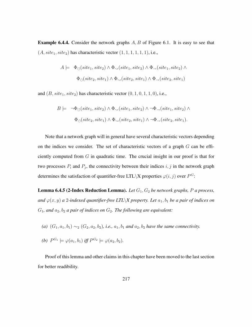
Example 6.4.4. Consider the network graphs A,B of Figure 6.1. It is easy to see that

(A, site1, site2) has characteristic vector (1, 1, 1, 1, 1, 1), i.e.,

A |= Φ(site1, site2) ∧ Φ;

(site1, site2) ∧ Φ→(site1, site2) ∧

Φ(site2, site1) ∧ Φ;

(site2, site1) ∧ Φ→(site2, site1)

and (B, site1, site2) has characteristic vector (0, 1, 0, 1, 1, 0), i.e.,

B |= ¬Φ(site1, site2) ∧ Φ;

(site1, site2) ∧ ¬Φ→(site1, site2) ∧

Φ(site2, site1) ∧ Φ;

(site2, site1) ∧ ¬Φ→(site2, site1).

Note that a network graph will in general have several characteristic vectors depending

on the indices we consider. The set of characteristic vectors of a graph G can be effi-

ciently computed from G in quadratic time. The crucial insight in our proof is that for

two processes Pi and Pj , the connectivity between their indices i, j in the network graph

determines the satisfaction of quantifier-free LTL\X properties ϕ(i, j) over P G:

Lemma 6.4.5 (2-Index Reduction Lemma). Let G1, G2 be network graphs, P a process,

and ϕ(x, y) a 2-indexed quantifier-free LTL\X property. Let a1, b1 be a pair of indices on

G1, and a2, b2 a pair of indices on G2. The following are equivalent:

(a) (G1, a1, b1) ∼2 (G2, a2, b2), i.e., a1, b1 and a2, b2 have the same connectivity.

(b) PG1 |= ϕ(a1, b1) iff PG2 |= ϕ(a2, b2).

Proof of this lemma and other claims in this chapter have been moved to the last section

for better readibility.

217

The lemma motivates the following model checking strategy: Given a (possibly com-

plicated) network graph G1 and two of its sites i, j, we can try to obtain a simpler network

G2 := G(i,j), with two special nodes site1 and site2 that have the same connectivity in G2

as the indices i and j in G1, and thus satisfies condition (a) of the lemma. For the case of

two indices, we can always find such a network graph G(i,j) with at most 4 sites.

Proposition 3. For each graph G and indices i, j there exists a 4-node graph G(i,j) called

the connection topology of i, j, having two special sites site1 and site2 such that

(G, i, j) ∼2 (G(i,j), site1, site2).

In other words, the indices i and j in G have the same connectivity as the indices site1 and

site2 in G(i,j).

Since G(i,j) satisfies condition (a) of Lemma 6.4.5, we obtain the following important

consequence:

Corollary 6. Let ϕ(i, j) be a 2-indexed quantifier-free LTL\X property. Then

PG |= ϕ(i, j) iff PG(i,j) |= ϕ(site1, site2).

Thus, we have achieved a reduction from a potentially large network graph G to a 4-

node network graph G(i,j). We will now show how to actually construct the connection

topology G(i,j).

Construction of G(i,j). We construct the reduction graphs as follows. G(i,j) has four

sites: site1, site2, hub1, and hub2. The sites site1 and site2 are called primary sites. They

represent the sites of interest i and j. The other sites are called hubs, and they represent

218

the other nodes of the graph G. Let us describe in more detail the role of these different

nodes. Recall that to satisfy Proposition 3, the sites site1 and site2 in G(i,j) should have

the same connectivity as i, j in G. Therefore:

• If Φ;

(i, j) holds in G (i.e., there exists a path from i to j in G that goes through a

third node), then Φ;

(site1, site2) has also to hold in G(i,j), i.e., there should exist

in G(i,j) a path from site1 to site2 that goes through a third node. The site hub1 will

play the role of this “third node”. Therefore, in this case, G(i,j) contains an edge

from site1 to hub1, and from hub1 to site2.

• In the same manner, if Φ(i, j) holds in G (i.e., there exists a path from i to itself

in G that does not go through j), then Φ(site1, site2) should also be true in G(i,j).

As previously, this is ensured by considering the following edges: (site1, hub1) and

(hub1, site1).

• Finally, if Φ→(i, j) holds in G (i.e., there exists a direct edge in G from i to j), then

G(i,j) should also contain the edge (site1, site2).

• The paths from j to i are treated in a symmetrical way.

For example, let H be a graph having as sites i, j, k, and l (among others), such that

v(H, i, j) = (1, 1, 1, 1, 1, 1), and v(H, k, l) = (0, 1, 0, 1, 1, 0); then the graphs A and B of

Example 6.4.4 correspond respectively to the reduction graphs H(i,j) and H(k,l).

Since our fairness assumption implies that the network is strongly connected, not all char-

acteristic vectors actually occur in practice. A closer analysis yields the following bound:

219

Proposition 4. For 2 indices, there exist at most 36 connection topologies.

All the 36 connection topologies are shown in the Section 6.8.

Let us now return to the question of verifying properties of the form ∃x, y.ϕ(x, y). Note

that Corollary 6 only provides us with a way to verify one quantifier-free formula ϕ(i, j).

Given a system PG, we define its 2-topology, denoted by T2(G), as the collection of all

different connection topologies appearing in G. Formally,

Definition 6.4.6. Given a network graph G = (S,C), the 2-topology of G is given by

T2(G) = G(i,j) | i, j ∈ S, i 6= j.

By Proposition 4, we know that |T2(G)| ≤ 36. Since we can express ∃x, y.ϕ(x, y) as a

disjunction∨i,j∈S ϕ(i, j) we obtain the following result as a consequence of Corollary 6:

Theorem 6.4.7. The following are equivalent:

(i) PG |= ∃x, y.ϕ(x, y)

(ii) There exists a connection topology T ∈ T2(G), such that P T |= ϕ(site1, site2).

Thus, we obtain the following reduction algorithm for model checking P G |= ∃x, y.ϕ(x, y):

1: Determine T2(G).

2: For each T ∈ T2(G), model check P T |= ϕ(site1, site2).

3: If one of the model checking calls is successful then output “true” else output

“false”.

220

Example 6.4.8.

Figure 6.2: A system with grid like network graph with 9 nodes.

Consider a system PG with a grid like network graph G shown in Figure 6.2. Assume

that each edge of the network is bidirectional. To verify a 2-indexed LTL \ X property

∃x, y.ϕ(x, y) of this system, it is enough to consider two systems P G1 and PG2 with net-

work graphs G1, G2 shown in Figure 6.3 and check ϕ(site1, site2) on each of them.

If either system satisfies ϕ(site1, site2) then PG |= ∃x, y.ϕ(x, y). Otherwise, it PG 6|=

∃x, y.ϕ(x, y).

Relation with Environment Abstraction

In this section we will consider the relationship between the decomposition presented here

and environment abstraction presented in the earlier chapters. For ease of comparison, we

will consider environment abstraction with single reference process and decompositions

221

site1

hub1

hub2

site2 site1

hub1

hub2

site2

Figure 6.3: Connection topologies for the grid-like network graph.

for two indexed properties.

First note that both the methods deal with properties of a fixed number of processes.

In the case of environment abstraction, we considered primarily single index properties,

that is, properties of one process and its environment. Here we consider double indexed

properties, that is properties satisfied by two processes and their common environment. To

build the abstract model in environment abstraction, we begin by asking how the system

looks when viewed from the reference process. The environment of the reference process

is captured using an appropriately chosen set of predicates. Our soundness theorem of

Chapter 2 shows that the abstract model built using these predicates is sound and our

experiments show that the abstract models are quite precise.

In this chapter too, we ask how the system looks like from the point of view of two

processes. But this time, the environment around the two processes is described mainly

in terms of the network topology. Note that the reduced system P G(i,j) corresponding to

processes i, j in a system PG can be thought of as an abstraction of PG. But, unlike

usual abstractions, the set of properties (involving only processes i, j) satisfied by P G(i,j)

222

is exactly the same as the set of properties satisfied by PG.

One way of looking at environment abstraction is to first consider the abstract models

obtained by fixing the reference process (as we do in the proof of soundness). That is, for

a given system P(K) consider the abstract models PA1 , . . . ,P

AK . If we can show, for each

i ∈ [1..K],

PAi |= Φ(i)

then we can conclude that

P(K) |= ∀x.Φ(x)

But, it is not feasible to check each of the abstract models PAi individually because there

is no bound on K. So instead of verifying each abstract model separately, we create a new

abstract model PA by combining all the individual models PA1 , . . . ,P

AK to obtain an even

more abstract model. By the existential abstraction principle, we have

PA |= Φ(x)⇒ ∀i.PAi |= Φ(i)

Thus, it is enough to verify the abstract model PA.

In contrast, in this chapter, we take every possible pair of processes i, j, and construct

the abstract model PG(i,j) specific to each of them. But then, instead of grouping all these

abstract models, we keep them separate and check each of them individually. This is pos-

sible because Proposition 4 guarantees that there are only 36 different possible reduction

graphs (or abstract models). This could not be done in the case of environment abstrac-

tion, because we don’t know apriori how many different individual abstract models are

there nor do we know how to find them efficiently.

223

To summarize, the reduction presented here and the environment abstraction both in-

volve describing the world around a fixed number of processes. Importantly, the results

presented in this chapter amount to reductions, that is , the properties under consideration

are preserved exactly. In contrast, in environment abstraction, the abstract model exhibits

more behaviors than the concrete system.

6.4.2 Existential k-indexed LTL\X Specifications

We will now show how to generalize the results of the previous section to k-indexed prop-

erties. Throughout this section, we will write expressions such as i to denote k-tuples of

indices, and x to denote k-tuples of variables. We will first adapt the notion of connectivity

as follows. Let i = i1, i2 . . . ik be a sequence of indices, and I = i1, i2 . . . ik. Then we

define the following connectivity properties:

G |= Φ(x, I) ”There is an (I \ x)-free path from x to itself.”

G |= Φ;

(x, y, I) ”There is a path from x to y via a third node not in I .”

G |= Φ→(x, y) ”There is a direct edge from x to y.”

By instantiating the variables x and y by the indices i1, . . . , ik in all possible ways, we ob-

tain a finite number of different conditions which will describe all possible connectivities

between the indices i1, . . . , ik.

As in the previous section, we can define an equivalence relation∼k, where (G1, i) ∼k

(G2, j) iff the indices i have the same connectivity in G1 as the indices j in G2. Since the

224

hub1site1

site2

site3

site4

site5

hub2

hub3

hub4

hub5

Figure 6.4: An example of a 5-index connection topology

number of conditions is bounded,∼k is an equivalence relation of finite index, and we can

describe each equivalence class by a characteristic vector v(G, v). As in the previous sec-

tion, we define the k-connection topologies, G(i1,i2...ik) of the processes Pi1 , Pi2 . . . Pik in

G as the smallest graphs that preserve all the connectivity properties between the processes

Pi1 , Pi2 . . . Pik . The construction of the topology graphs is illustrated in Figure 6.4.

The unfilled nodes site1, . . . , sitek in the graph are the primary sites. There is a hub

site associated with each primary site. Moreover, there is an edge from each hub hubj

back to its primary sitej if there is an (I \ij)-free path from ij to itself. There is an edge

from hubj to sitel if there is a path from ij to il in G via a third node not in I , and there is

an edge from sitej to sitel if there exists a direct edge (ij, il) in G.

Analogous to the bounds on 2-connection topologies it can be shown that each k-

connection topology has at most 2k processes and that there are at most 3k(k−1)2k distinct

k-connection topologies. By an argument analogous to that of the previous section, we

obtain the following corollary

225

Corollary 7. Let ϕ(x) be a k-indexed quantifier-free LTL\X property. Then

PG |= ϕ(i) iff PG(i) |= ϕ(site1, site2, . . . , sitek).

The notion of k-topology is defined analogously:

Definition 6.4.9. Given a network graph G = (S,C) the k-topology of G is given by

Tk(G) = G(i) | i ∈ Sk, all indices in i are distinct.

Consequently, we obtain a model checking procedure from the following theorem,

similar to the case of 2-indices:

Theorem 6.4.10. The following are equivalent:

(i) PG |= ∃x.ϕ(x)

(ii) There exists a connection topologyT ∈ Tk(G), such thatP T |= ϕ(site1, site2, . . . , sitek).

As mentioned before |Tk(G)| ≤ 3k(k−1)2k.

6.4.3 Specifications with General Quantifier Prefixes

In this section we will show how to obtain reductions for k-indexed specifications with

first order prefixes.

Let us for simplicity consider the 2-indexed formula Φ := ∀x∃y.ϕ(x, y). Over a

network graph G = (S,C), |S| = n, it is clear that Φ is equivalent to ∧1≤i≤n ∨1≤j≤n

ϕ(i, j). A naive application of Corollary 7 would therefore require n2 calls to the model

226

checker, which may be expensive for practical values of n. In practice, however, we can

bound the number of model checker calls by |T2(G)| since this is the maximum number of

different connection topologies. We conclude that the n2 model checker calls must contain

repetitions. We can make sure that at most 36 calls to the model checker are needed. We

obtain the following algorithm:

1: Determine T2(G).

2: For each T ∈ T2(G)

3: model check P T |= ϕ(site1, site2)

4: g[T ] := 1 iff model checking successful, and 0 otherwise

5: Output∧

1≤i≤n

∨1≤j≤n g[G(i,j)].

By simplifying the formula in line 5, we may further increase performance. The algo-

rithm can be adapted for k indices in the obvious way. To state the main theorem of this

section, we define (c, s)-bounded reductions, where c bounds the number of calls to the

model checker, and s bounds the size of the network graph.

Definition 6.4.11 ((c, s)-bounded Reduction). Let G, P be as above, and ϕ be a closed

k-indexed formula with matrix ϕ′(x1, . . . , xk). Let Ψ denote a property of interest (e.g.,

the model checking property ′′PG |= ϕ′′). A (c, s)-bounded reduction of property Ψ is

given by:

• a sequence of c reduced network graphs Gi = (Si, Ci), 1 ≤ i ≤ c such that |Si| ≤ s.

called reduction graphs.

227

• a boolean function B over c variables g1, . . . , gc, such that

Ψ iff B(g1, . . . , gc) = 1 where gi := 1 iff GPi |= ϕ′(site1, . . . , sitek)

In other words, property Ψ is decided by c calls to the model checker, where in each

call the network graph is bounded by s.

Further, we say that a class L of specifications has (c, s) bounded reduction if for all

network graphs G and any ϕ ∈ L, the property PG |= ϕ has (c, s)-bounded reduction. We

can now state our main result:

Theorem 6.4.12. Let ϕ be any k-indexed LTL\X specification. Then the model checking

problem ′′PG |= ϕ′′ has polynomial-time1 computable (3k(k−1)2k, 2k)-bounded reductions.

In fact, the sequence of reduced network graphs is just the different k-connection topolo-

gies occurring in G. This implies that given k and network graph G, all k-indexed LTL\X

specifications have the same reduction. Stated another way, LTL\X has (3k(k−1)2k, 2k)-

bounded reduction.

6.4.4 Cut-Offs for Network Topologies

In this section, we prove the existence of cutoffs for network topologies, i.e., (infinite)

classes of network graphs. We say that a class of network graphs has cutoff (c, s), if the

question whether all the network graphs in this topology satisfy the specification has a

(c, s)-bounded reduction.

1in the size of the network graph G

228

Definition 6.4.13 (Cut-off). Let T be a network topology, and L a class of specifications.

T has a cut-off (c, s) for L if for all specifications ϕ ∈ L the property

Ψ := “ ∀G ∈ T . PG |= ϕ ”

has a (c, s)-bounded reduction.

It is not hard to prove that a (c, s)-bounded reduction for a network graph translates to

a cut-off for a network topology:

Theorem 6.4.14. For k-indexed specifications, all network topologies T have (2k, 3k(k−1)2k)-

bounded reductions.

Note that the theorem does not provide us with an effective means to find the reduc-

tion; it does however guarantee that at least in principle we can always find a cutoff by

investigating the topology T.

6.5 Bounded Reductions for CTL\X are Impossible

In this section, we show that indexed CTL\ X formulas over two indices do not have

(c, s)-bounded reductions. We will first show the following generic result about CTL\ X:

Theorem 6.5.1. For each number i there exists an CTL\ X formula ϕi with the following

properties:

• ϕi is satisfiable (and has a finite model).

• ϕi uses only two atomic propositions l and r.

229

• Every Kripke structure K where ϕi is true has at least i states.

• ϕi has the form EFϕ′i.

The result is true even when the Kripke structure is required to have a strongly con-

nected transition relation.

Remark 15. This result is closely related to early results about characterizing Kripke

structures up to bisimulation in [14]. The results in [14] give rise to the following proof

idea for Theorem 6.5.1: Let K1, . . . , Kn be all Kripke structures with 2 labels of size

≤ i, and let f1, . . . , fn be CTL\ X formulas which characterize them up to stuttering

bisimulation. Consider now the formula ϕi :=∧

1≤j≤n ¬fj . By construction every model

of ϕi must have > i states. At this point, however, the proof breaks down, because we

do not know from the construction if ϕi is satisfiable at all. The natural way to show that

ϕi has a model would be to prove that stuttering bisimulation over a 2-symbol alphabet

has infinite index. This property however is a corollary to Theorem 6.5.1, and we are not

aware of a proof in the literature.

For properties involving only the presence of the token, a system P G, where G =

(S,C) essentially behaves like a Kripke structure with set of states S and transition relation

C. To see this, consider a system PG, where P is a trivial process which can always

receive a token, and immediately send the token to a neighbor process. Let ti and tj be

propositional formulas stating that the token is with process i and j respectively. Since the

processes do not influence the path taken by the token, the token moves only according to

the network graph G, and thus for each path on PG there exists a corresponding path in G.

Consequently, if a path on PG satisfies a property without X, then the corresponding path

230

on G also satisfies this property. Now we can show by contradiction that indexed CTL\ X

cannot have bounded reductions. Suppose CTL\X did have (c, s)-bounded reduction for

some s. Then, by Theorem 6.5.1, we can always find a CTL\X formula Φ such that the

network graph underlying any system that satisfies Φ must have size at least c + 1. Thus

CTL\X does not have bounded reductions. Consequently, we also have the following

corollary:

Corollary 8. There exists a network topology T for which 2-indexed CTL\ X does not

have cut-offs.

A detailed proof can be found in the last section of this chapter.

6.6 Conclusion

We have described a systematic approach for reducing the verification of large and pa-

rameterized systems to the verification of a sequence of much smaller systems. We will

conclude this chapter with further considerations concerning the practical complexity of

model checking.

For simplicity, let us again consider the case of 2-indexed properties. Suppose the

processes P in our network have state space |Q|. Then our reduction requires to model

check up to 36 network graphs with 4 sites, resulting in a state space of |Q|4 . Even this

model checking problem may be too expensive in practice. By a close analysis of our

proofs, it is however possible to reduce the state space even further to O(|Q|2).

It is easy to show that Lemma 6.4.5 will hold even when the processes at the hubs

231

are simple dummy processes containing two states whose mere task is to send and receive

the token infinitely often. Consequently, the systems P G(i,j) will have state space of size

22 × |Q|2.

The results in this chapter on LTL\X were derived assuming fairness condition on the

systems. We can obtain similar reductions by removing this assumption. Doing away

with fairness necessitates the consideration of two more path types other than the ones

described in Section 6.4.1. Consequently, the topology graphs have more than 4 sites and

also the number of different topology graphs increases.

6.7 Proofs of Lemmas

Proposition 4. For 2 indices, there exist at most 36 connection topologies.

Proof. By our fairness assumption, every connection topology must be strongly con-

nected. This implies that the following conditions must hold:

• At least one of Φ→(i, j) or Φ;

(i, j) must be true.

• At least one of Φ→(j, i) or Φ;

(j, i) must be true.

This means in the characteristic vector of connection topology the following must hold:

• At least one of the second and third elements (corresponding to the connectivity

properties discussed above) must be 1. This gives us three choices in picking the

second and third elements of the vector.

232

• At least one of the fifth and sixth elements must be 1. This again gives us three

choices in picking the fifth and the sixth elements of the vector.

• First and fourth elements can be either 0 or 1. This gives us four choices in picking

the first and the fourth elements of the vector.

Consequently the number of different possible characteristic vectors is 3 × 3 × 4 =

36.

Lemma 6.4.5. Let G1, G2 be network graphs, P a process, and ϕ(x, y) a 2-indexed

quantifier-free LTL\X property. Let a1, b1 be a pair of indices on G1, and a2, b2 a pair

of indices on G2. The following are equivalent:

(a) (G1, a1, b1) ∼2 (G2, a2, b2), i.e., a1, b1 and a2, b2 have the same connectivity.

(b) PG1 |= ϕ(a1, b1) iff PG2 |= ϕ(a2, b2).

We first define some notions which will be helpful in proving the lemma. Let P G be a

system with m processes

An execution trace of the system PG is a series of global states in such that

there is a transition from every kth state in the trace to the (k + 1)th state.

Given a trace t, we will denote the nth state in t by tn.

A witness in system PG for a LTL \ X formula ϕ(i, j) (where Pi and Pj

are two processes in G) is an execution trace of S that satisfies the LTL \X

formula.

233

We now define the projection of an execution trace with respect to a set of indices I =

i1, . . . ik. First we describe the collapse of a trace with respect to I .

Definition 6.7.1. Given an execution trace t of a system P G and a set of indices I , the

collapse of t with respect to I is obtained by removing every global state, tn+1 in t such

that ∀i ∈ I.tn(i) = tn+1(i)

Informally, a collapse of trace t is obtained by removing those global states from the

trace which do not change the states of processes with indices I .

Definition 6.7.2. Given a collapsed trace tc of PG with respect to I the projection of t

with respect to I is the series of states obtained by projecting each global state in tc onto

the processes in I .

Lemma 6.7.3. If two execution traces, t1 and t2 have the same projection with respect to

a set of processes, I , then the two traces satisfy exactly the same set of LTL\X properties

over I .

Proof. This follows from the semantics of LTL \X properties.

Lemma 6.7.4. A system PG with two indices i and j satisfies an LTL\X property ϕ(i, j)

if and only if the system PG(i,j) satisfies the property ϕ(site1, site2).

Proof. We will prove that if PG satisifes a propertyϕ(i, j) then PG(i,j) satisfiesϕ(site1, site2).

The proof for the other direction is exactly the same.

Consider any two-indexed LTL \ X property ϕ(i, j). Let system P G satisfy ϕ(i, j).

Consider a witness, w, for ϕ(i, j) in the system S. Obtain the projection, wp, of w with

234

respect to indices i, j. Note that each state in wp will be of the form (qi, qj) where qi, qj

are local states of processes i, j respectively.

We will say a trace w′ of PG(i,j) matches wp if the projection of w′ with respect to in-

dices site1 and site2 is isomorphic to wp modulo renaming. Clearly, if a trace w′ matching

wp exists in PG(i,j) then the system PG(i,j) satisfies the property ϕ(site1, site2).

We will now construct a trace w′ of PG(i,j) that matches wp. The state of process i in

PG will be matched by the state of process site1 in PG(i,j) and the state of process j will be

matched by the state of process site2. Consider the first state (qi, qj) of the trace wp. Since

(qi, qj) is the first state of the trace wp, both qi, qj must be the initial local states. The first

state of w′ will then be (qsite1 , qhub1 , qsite2 , qhub2) where qsite1 , qsite2 are initial local states.

The hubs can be in any local state, so by default we require them to be in initial states as

well.

The token could be held in three possible ways the state (qi, qj):

• By process i.

• By process j.

• By neither i nor j

In case the token is with process i then in w′ the token will be with process site1. In

case the token is with process j then in w′ the token will be with process site2. In the last

case, the first global state of w′, (qsite1 , qhub1 , qsite2 , qhub2), is such that token is with qhub1

or qhub2 . It is easy to see that the first state of w′ thus constructed matches the first state of

wp.

235

Assume that we have been able to construct a prefix pf of w ′ which matches the prefix

ofwp of length k. Denote themth state inwp bywmp and the prefix of lengthm bym-prefix.

To extend the trace w′ to k + 1 states consider the states wkp and wk+1

p of wp. We have

the following cases to consider:

• In going from wkp to wk+1

p there is no change in the process holding the token. As-

sume, without loss of generality, that the difference betweenwkp andwk+1

p is a change

in the local state of process i. Consider w′k, the kth state of w′. Since w′ matches

the k-prefix of wp, the states of process i in wkp and process site1 in w′k must match.

This means whatever action i can take, the same action can be taken by site1. Thus,

we can extend w′ to k + 1 states by replicating the action of process i using process

site1.

• In wkp the token is with i and in wk+1

p is with j. We can then infer that there must be a

direct edge in G from process i to j, that is, G |= Φ→(i, j) must be true. Thus there

must be a similar direct edge inG(i,j) from site1 to site2, that is in G(i,j) |= Φ→(i, j)

is true. And since the prefix pf of w′ matches the k-prefix of wp, in the last state of

pf , w′k, the token must be with process site1. Further, the states of site1 and site2

in w′k must be the same as the states of i and j (respectively) in wkp . Thus, we can

extend w′ with the state that is obtained by a token transfer from site1 to site2. Thus

we have a prefix of w′ that matches the k + 1-prefix of wp. The case where token is

with j in wkp and with i in wk+1

p is analogous.

• In wkp the token is with neither i nor j and in wk+1

p it is with j. This case has the

following three sub-cases

236

– In the k-prefix of wp the token was last with j. That is, there is a state wmp ,

m < k such that the token is with process j in wmp and in no state wn

p , m <

n ≤ k is the token with either process i or j.

This implies that there a path from j to itself in G that does not go through i,

that is G |= Φ(j, i). Then there must be a similar path from site2 to itself in

G(i,j) which does not go through site1, that is, G(i,j) |= Φ(site2, site1) must

hold. Since pf matches k-prefix of wp, the process that last had the token in pf

must be site2. In the last state l of pf the token is neither with site1 or site2.

We can infer that the token must be with process hub2 because site2 can send

token to either site1 or hub2 and the token is not with site1. Then we can add

a series of states to pf such that, at the end, token is transferred back to site2

and the only process that changes the state in this series of states prior to token

transfer is hub2. This is always possible because of our assumption that each

process can send and receive token infinitely often. Thus we now have prefix

of w′ that can match the first k + 1 states of wP .

– In the k-prefix of wp the token was last with i. This means that there a path

from i to j in G that goes through a third process, that is Φ;

(i, j) must hold

in G. Then there must be a similar path from site1 to site2 in G(i,j) that goes

through hub1. In the last state l of pf the token is with hub1. To see this, note

that site1 can send token either to hub1 or site2 and in l the token cannot be

with site2 (otherwise pf will not match the k-prefix of wp). As before, we can

add a series of states to pf such that at the end token is with site2 and the only

process that changes state prior to token transfer is process hub1.

237

– In the k-prefix of wp the token was never with i or j. That is wk+1p is the first

state where the token is with j. We have constructed pf such that it matches

the k-prefix of wp. Since there was no token transitions involving either i or

j, all the transitions in pf must have been transitions local to i or j. Thus, it

does not matter where the token was initially in pf . Since we are interested

only in existential properties, we can construct pf such that the token is with

process hub2 in the last state l. This means that from l we can have a token

transition from process hub2 to site2. Thus we can extend pf so that it matches

k + 1-prefix of wp.

The case where the token is with neither i nor j in the state wkp and with i in the state

wk+1p is analogous.

Thus, we can construct a trace of w′ of S ′ which matches wp.

Note that we have implicitly used the fairness assumption for P G. The assumption is

implicit in the fact there is always a k + 1th state in pf that is to be matched.

Lemma 6.7.5. Let PG1 and PG2 be two systems. Further let there be two processes

indexed i and j in both G1 and G2. If for all two indexed LTL \ X property ϕ(i, j),

PG1 |= ϕ(i, j)⇔ PG2 |= ϕ(i, j) then G1(i,j)= G2(i,j)

.

Proof. The proof strategy is the following. For each path-type, we will give a two-indexed

LTL \ X formula Ψ(i, j) such that if Ψ(i, j) holds on a system PG then the associated

path-type exists between i and j in the network G.

238

The three formulas are:

• For Φ(i): F (ti ∧ (¬tj U ¬(ti ∨ tj)) U ti)

• For Φ;

(i, j): F (ti ∧ (¬tj U ¬(ti ∨ tj)) U tj)

• For Φ→(i, j): F (ti ∧ (ti U tj))

It is easy to see that each of the three formulas implies the associated path type.

Now if PG1 satisfies exactly those two-indexed properties as PG2 , then the two systems

must satisfy exactly the same type formulas. Hence G1(i,j)= G2(i,j)

Lemma 6.4.5. We first prove that (i) ⇒ (ii). Assume that (G1, a1, b1) ∼2 (G2, a2, b2).

Then we know that

G1(a1,b1)= G2(a2,b2)

.

By Lemma 6.7.5,

PG1 |= ϕ(a1, b1)

⇔ PG1(a1,b1) |= ϕ(site1, site2)

⇔ PG2(a2,b2) |= ϕ(site1, site2)

⇔ PG2 |= ϕ(a2, b2).

For the other direction, assume PG1 |= ϕ(a1, b1)⇔ PG2 |= ϕ(a2, b2). Now,

PG1 |= ϕ(a1, b1)⇔ PG1(a1,b1) |= ϕ(site1, site2)

239

and

PG2 |= ϕ(a2, b2)⇔ PG2(a2,b2) |= ϕ(site1, site2).

Thus

PG1(a1,b1) |= ϕ(site1, site2)⇔ P

G2(a2,b2) |= ϕ(site1, site2)

which implies, by Lemma 6.7.4, that G1(a1,b1)= G2(a2,b2)

and therefore(G1, a1, b1) ∼2

(G2, a2, b2).

Theorem 6.4.14 For k-indexed specifications, all network topologies T have (2k, 3k(k−1)2k)-

bounded reductions.

Proof. Let ϕ be a k-indexed specification and G1, G2, . . . be an enumeration of the net-

work graphs in T. Since model checking for each graphGi ∈ T is (2k, 3k(k−1)2k)-bounded

regardless of the size of Gi, we obtain a sequence of Boolean functions Bi over the same

variables g1, . . . , g3k(k−1)2k . Consider now the (infinitary) conjunction B :=∧i≥1Bi. By

Corollary 7, the function B expresses that for all Gi we have GPi |= ϕ. It remains to

show that Ψ is equivalent to a finite formula. Since B depends only on a finite number

(3k(k−1)2k) of Boolean variables, functional completeness of Boolean logic implies that B

is equivalent to a finite formula of size at most 23k(k−1)2k .

Theorem 6.5.1. For each number i there exists a CTL\X formula ϕi with the

following properties:

• ϕi is satisfiable (and has a finite model).

240

• ϕi uses only two atomic propositions l and r.

• Every Kripke structure K where ϕi is true has at least i states.

• ϕi has the form EFϕ′i.

The result remains true, when the Kripke structure is required to have a strongly con-

nected transition relation.

Proof. Our goal is to describe a formula ϕi using atomic propositions l and r whose mod-

els must have at least i states. We will construct a large conjunction∧ψ∈Γ ψ, and describe

which formulas to put in Γ. The idea is simple: Γ needs to contain i CTL\X formulas

which describe the existence of i different states. Then the formula EF∧ψ∈Γ ψ will be the

sought for ϕi.

Consider a Kripke structure K as in Figure 6.5:

• In Level 0, it contains two distinct states L,R labelled with l and r respectively. To

express the presence of these states, we include the formulas, let ψ10 := (l ∧¬r) and

ψ20 := (r ∧ ¬l), and include EFψ1

0 and EFψ20 into Γ.

It is clear that EFψ10 and EFψ2

0 express the presence of two mutually exclusive

states.

• In Level 1, K contains 22 − 1 = 3 states, such that the first one has L,R-free

paths to L and R, the second one an L,R-free path only to L, and the third one

an L,R-free path only to R. The characteristic properties of level 1 states are

expressed by formulas

241

L

R

Level 0Level 1Auxilliary Node Level 2

Figure 6.5: The Kripke structure K, constructed for three levels. The dashed lines indicate the connections

necessary to achieve a strongly connected graph.

ψ11 := EF−ψ1

0 ∧ EF−ψ20

ψ21 := EF−ψ1

0 ∧ ¬EF−ψ20

ψ31 := ¬EF−ψ1

0 ∧EF−ψ20

where EF−x denotes E(¬l ∧ ¬r)Ux, i.e., a variant of EF which forbids paths

through L and R. To enforce the existence of the Level 1 states in the Kripke struc-

ture, we include EFψ11,EFψ2

1,EFψ31 into Γ.

• In Level 2, K contains 23 − 1 = 7 states, such that every state in level 2 can reach

one of the 7 non-empty subsets of Level 1. The characteristic properties of Level 2

states can be expressed by formulas such as

ψ12 := EF−ψ1

1 ∧ EF−ψ21 ∧ EF−ψ3

1

242

and

ψ22 := ¬EF−ψ1

1 ∧EF−ψ21 ∧EF−ψ3

1

, etc including ψ32 to ψ7

2 . To enforce the presence of Level 2 states in the Kripke

structure, we include the formulas EFψi2 for i = 1, . . . , 7 into Γ.

• In general, each Level k has at least 2k+1 − 1 states that differ in their relationship

to the states in Level k − 1. The presence of such states is expressed by formulas

EFψxk .

All these formulas are included into Γ until the requested number i of different states is

reached. By construction, all properties required by the theorem are trivially fulfilled. In

particular, Figure 6.5 demonstrates that there always exists a strongly connected model.

The formula ϕi uses two labels l, r. To use the above theorem in the setting of systems

with network graphs, we replace the labels l, r by atomic propositions tx, ty. Recall that an

atomic proposition tx states that the token is with process x. We will denote the modified

formula by ϕi(x, y). We have the following proposition as a consequence of the above

theorem.

Corollary 9. If PG |= ∃x, y. ϕi(x, y), where G = (S,C) then |S| > i.

Proof. Consider formula ∃x, y.ϕi(x, y) and suppose, towards a contradiction, that there

is a system PG, G = (S,C) where |S| < i such that PG |= ∃x, y.ϕi(x, y). Then there

exist indices a, b such that PG |= ϕi(a, b). We construct the Kripke structure K with state

space S, transition relation C, initial state 1, and two atomic propositions ta, tb which hold

243

true on states a and b respectively. Note that since the formula ϕi(a, b) is of the form

EFϕ′i(a, b) and C is strongly connected, satisfaction of ϕi(a, b) does not depend on the

choice of the initial state. Since we know that for all paths on P G, the corresponding paths

on G preserve properties without X, it follows that K |= ϕi(a, b). By the above theorem,

K must have at least i states, which contradicts our assumption that |S| < i. Thus, we

have a proof by contradiction that if PG |= ∃x, y.ϕi(x, y) then the network graph G must

have at least i nodes in it.

Corollary 8. There exists a network topology T for which 2-indexed CTL \ X

does not have cut-offs.

Proof. Let T be the class of strongly connected graphs. Then Corollary 9 tells us that

∃x, y.ϕn(x, y) does not have a cut-off for T.

6.8 Connection Topologies for 2-Indices

All the 36 possible connection topologies between two processes are presented below.

244

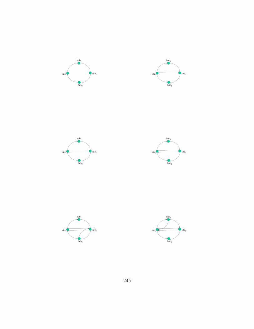
site1

hub1

hub2

site2 site1

hub1

hub2

site2

site1

hub1

hub2

site2 site1

hub1

hub2

site2

site1

hub1

hub2

site2 site1

hub1

hub2

site2

245

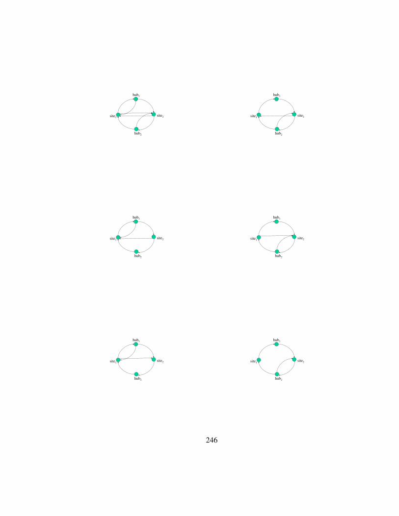
site1

hub1

hub2

site2 site1

hub1

hub2

site2

site1

hub1

hub2

site2 site1

hub1

hub2

site2

site1

hub1

hub2

site2 site1

hub1

hub2

site2

246

site1

hub1

hub2

site2 site1

hub1

hub2

site2

site1

hub1

hub2

site2 site1

hub1

hub2

site2

site1

hub1

hub2

site2 site1

hub1

hub2

site2

247

site1

hub1

hub2

site2 site1

hub1

hub2

site2

site1

hub1

hub2

site2 site1

hub1

hub2

site2

site1

hub1

hub2

site2 site1

hub1

hub2

site2

248

site1

hub1

hub2

site2 site1

hub1

hub2

site2

site1

hub1

hub2

site2 site1

hub1

hub2

site2

site1

hub1

hub2

site2 site1

hub1

hub2

site2

249

site1

hub1

hub2

site2 site1

hub1

hub2

site2

site1

hub1

hub2

site2 site1

hub1

hub2

site2

site1

hub1

hub2

site2 site1

hub1

hub2

site2

250

Chapter 7

Conclusion

7.1 Summary

This thesis presents an efficient abstraction technique to facilitate model checking of

parameterized systems with replicated processes. All successful applications of model

checking thus far have made use of domain specific abstraction techniques. Continuing

this trend, we exploit the domain knowledge about parameterized systems to devise an

appropriate abstraction method.

The problem of verifying parameterized systems is both challenging theoretically (be-

cause of their unboundedness) and very relevant practically (because many crucial com-

ponents of real systems are parameterized). For example, in the recent years, verification

of cache coherence protocols has become a very important problem in the hardware indus-

try. All the modern multi-core architectures have very intricate cache coherence protocols,

251

and there are no rigorous techniques for their verification. Similarly, the number of con-

trollers used in embedded applications, for example on automobiles, is also increasing,

and, to facilitate efficient communication between the controllers, complex time triggered

protocols are being developed. These protocols are also parameterized as the number of

controllers can vary. As with cache coherence protocols, there are no efficient automated

techniques for verifying these protocols. To model check complex protocols like these, we

need efficient abstraction techniques.

In this thesis, we present an abstraction method called environment abstraction for

verifying parameterized systems with replicated processes. The main insight in this tech-

nique is that, when a human designer reasons about a system with replicated components,

(s)he tends to focus on a reference component and consider the environment around it.

We formalize this insight and provide a rigorous framework for constructing such abstract

models. The abstract models are quite precise and easy to construct. In most abstraction

methods, liveness properties are more difficult to handle, even theoretically, than safety

properties. Our method, however, has a simple extension to handle liveness properties.

Finally, most automatic abstraction based methods for verifying parameterized systems

use the atomicity assumption. In contrast, we are able to remove the atomicity assumption

by adding monitor processes and, thus, verify protocols in their full generality. Our ex-

periments with different cache and mutual exclusion protocols suggest that environment

abstraction works extremely well in practice.

The insight of constructing an abstract model by considering one reference process

and looking at the world around it can be generalized to different settings. Instead of just

considering a collection of processes, each of which can talk with every other process,

252

we consider a richer model in which processes are arranged on the nodes of a network

graph. Thus, in addition to replication of processes, we also have an arbitrary network

graph to reason about. This problem structure is quite common in real life. For instance,

network routing protocols, which route data through complicated networks of machines,

have to function no matter what the structure of the network. Each of these machines runs

the exact same routing protocol. While there has been work on verifying systems with

replicated processes, there has not been much work on verifying systems with network

graphs. In Chapter 6, we take the first steps towards verifying parameterized systems

with network graphs. We consider the verification of two process properties and show

how to decompose a system with a large network to a collection of systems with constant

sized network graphs. The main idea is that it suffices to consider how the network looks

from a pair of processes to figure out what properties the pair satisfies. It can also be

shown that, for any pair of processes, there are only a finite number of possibilities for

how the network around them can look like. The results presented in Chapter 6 also

highlight an interesting contrast in the expressive power of LTL and CTL specifications.

We show that, while decomposition of large network into smaller ones is possible for

LTL specifications, it is not possible for CTL specifications. Informally, two process CTL

specifications can encode information about the number of other processes in the system

and, thus, decomposition is not possible for CTL properties.

253

7.2 Extensions

In this thesis, we considered parameterized systems with replicated processes. Environ-

ment abstraction is quite general and can be applied even when the replicated components

are not processes or if there are multiple types of replication. For instance, we can think

of a memory bank as a collection of identical components (ignoring the contents of the

memory). Similarly, we can treat a collection of jobs waiting to be scheduled in a queue

as an instance of replication (ignoring the specifics of the job). We believe this viewpoint

will lead to useful abstractions.

The abstract model that we construct is doubly exponential in the number of local state

variables. In real cache coherence protocols, the internal state of each cache can be quite

complex and thus our method might fail. To get around this, the internal states of local

caches themselves might have to be abstracted before applying environment abstraction.

An interesting extension to our work would be to combine environment abstraction with

standard abstraction for the internal states of the caches.

Our work in Chapter 6 lays the foundational results for the verification of parame-

terized systems with network graphs. While the system model does consider a network

graph, the communication between the processes is very simple. An extension to our work

would be to consider richer communication between processes. However, we suspect that

the decomposition results may not exist even for LTL properties once we allow more than

one token. It would be interesting to consider what restrictions to impose on the system

model so that we can still obtain decomposition results.

The abstraction based approach we have presented for verification of parameterized

254

systems is just one possible approach. In most real world parameterized systems, it seems

to be the case that, all possible two process behaviors are exhausted when the parameter

value is just 4 or 5. If such a cutoff really exists, then parameterized verification is no

different from ordinary verification. But, finding such cutoffs is very hard and no such

cutoffs are currently known. A related idea is to determine cutoff on trace length: it would

be extremely useful in practice if we can show that all interesting behaviors are exhibited

by traces of length less than a certain cutoff c. For instance, we could use bounded model

checkers, which are typically faster than the other types of model checkers, to explore the

parameterized system up to depth c. If no bug is found, then our cutoff result ensures that

the parameterized system is correct. While it seems such trace cutoffs must exist, no one

has succeeded in finding them yet. Finding cutoff results is a challenging problem with

significant practical impact.

Distributed and parallel systems are among the hardest systems for humans to rea-

son about. Yet parallelism seems to afford the easiest route to scalability and increased

performance. Consequently, highly parallel, distributed computer systems are becoming

quite pervasive. Powerful verification techniques are required to ensure the correct func-

tioning of these systems. Model checking, which performs an exhaustive search of the

state space, seems ideally suited for verification of distributed systems. In this thesis, we

have addressed the problem of model checking distributed protocols like cache coherence

protocols and mutual exclusion and demonstrated that it is possible to efficiently and au-

tomatically model check such protocols in their full generality.

255

Bibliography

[1] P. A. Abdulla, B. Jonsson, M. Nilsson, and J. d’Orso. Regular Model-Checkingmade Simple and Efficient. In Proceedings of the 13th International Conference onConcurrency Theory (CONCUR), 2002.

[2] K. Apt and D. Kozen. Limits for Automatic Verification of Finite State ConcurrentSystems. Information Processing Letters, 15:307–309, 1986.

[3] T. Arons, A. Pnueli, S. Ruah, and L. Zuck. Parameterized Verification with Auto-matically Computed Inductive Assertions. In Proceedings of the 13th InternationalConference on Computer Aided Verification (CAV), 2001.

[4] Thomas Ball and Sriram K. Rajamani. Boolean Programs: A Model and Process forSoftware Analysis. Technical Report MSR-TR-2000-14, Microsoft Research Corpo-ration, 2000.

[5] Tom Ball, Sagar Chaki, and Sriram Rajamani. Verification of Multi-Threaded Soft-ware Libraries. In Proceedings of the 23rd International Conference on SoftwareEngineering (ICSE), 2001.

[6] K. Baukus, S. Bensalem, Y. Lakhnech, and K. Stahl. Abstracting WS1S Systems toVerify Parameterized Networks. In Proceedings of the 6th International Conferenceon Tools and Algorithms for Construction and Analysis of Systems (TACAS), 2000.

[7] K. Baukus, Y. Lakhnech, and K. Stahl. Verification of Parameterized Protocols. InJournal of Universal of Computer Science, 2001.

[8] Armin Biere, Alessandro Cimatti, Edmund M. Clarke, Masahiro Fujita, and YunshanZhu. Symbolic Model Checking using SAT Procedures instead of BDDs. In Pro-ceedings of the ACM/IEEE Design Automation Conference (DAC), pages 317–320,1999.

257

[9] Jesse Bingham and Alan Hu. Empirically Efficient Verification for a Class of InfiniteState Systems. In Proceedings of the 11th International Tools and Algorithms forConstruction and Analysis of Systems (TACAS), 2005.

[10] B. Boigelot, A. Legay, and P. Wolper. Iterating Transducers in the Large. In Pro-ceedings of the 15th International Conference on Computer Aided Verification (CAV).LNCS, Springer-Verlag, 2003.

[11] A. Bouajjani, P. Habermehl, and T. Vojnar. Verification of Parametric ConcurrentSystems with Prioritized FIFO Resource Management. In Proceedings of 14th Inter-national Conference on Concurrency Theory (CONCUR), 2003.

[12] A. Bouajjani, B. Jonsson, M. Nilsson, and T. Touili. Regular Model Checking. InProceedings of the 12th International Conference on Computer Aided Verification(CAV). LNCS, Springer-Verlag, 2000.

[13] A. Bouajjani and T. Touili. Extrapolating Tree Transformations. In Proceedingsof the 14th International Conference on Computer Aided Verification (CAV). LNCS,Springer-Verlag, 2002.

[14] M. C. Browne, E. M. Clarke, and O. Grumberg. Characterizing Finite Kripke Struc-tures in Propositional Temporal Logic. Theoretical Computer Science, 59:115–131,1988.

[15] M. C. Browne, E. M. Clarke, and O. Grumberg. Reasoning about Networks withMany Identical Finite State Processes. Information and Computation, 81:13–31,1989.

[16] Randal E. Bryant. Graph-based Algorithms for Boolean Function Manipulation.IEEE Transactions on Computers, C-35(8):677–691, August 1986.

[17] Randal E. Bryant, Shuvendu K. Lahiri, and Sanjit A. Seshia. Deciding CLU LogicFormulas via Boolean and Pseudo-Boolean Encodings. In Proceedings of Interna-tional Workshop on Constraints in Formal Verification, 2002.

[18] Randal E. Bryant, Shuvendu K. Lahiri, and Sanjit A. Seshia. Modeling and VerifyingSystems using a Logic of Counter Arithmetic with Lambda Expressions and Uninter-preted Functions. In Proceedings of the 14th International Conference on ComputerAided Verification (CAV), 2002.

258

[19] Sagar Chaki, Edmund Clarke, ALex Groce, Somesh Jha, and Helmut Veith. ModularVerification of Software Components in C. In Proceedings of the 25th InternationalConference on Software Engineering (ICSE), pages 385–395, 2003.

[20] Prosenjit Chatterjee, Hemanthkumar Sivaraj, and Ganesh Gopalakrishnan. SharedMemory Consistency Protocol Verification against Weak Memory Models: Refine-ment via Distributed Model Checking. In Proceedings of the 14th InternationalConference on Computer Aided Verification (CAV), 2002.

[21] Ching-Tsun Chou, Phanindra K. Mannava, and Seungjoon Park. A Simple Methodfor Parameterized Verification of Cache Coherence Protocols. In Proceedings of the5th International Conference on Formal Methods in Computer-Aided Design (FM-CAD), 2004.

[22] E. Clarke, O. Grumberg, S. Jha, Y. Lu, and H. Veith. Counterexample-Guided Ab-straction Refinement. In Proceedings of the 12th International Conference on Com-puter Aided Verification (CAV), 2000.

[23] E. Clarke, O. Grumberg, and D. Long. Model Checking and Abstraction. In Proceed-ings of the 19th ACM Symposium on Principles of Programming Languages (POPL),1992.

[24] E. M. Clarke, T. Filkorn, and S. Jha. Exploiting Symmetry in Temporal ModelChecking. In Proceedings of the 5th International Conference on Computer AidedVerification (CAV), 1993.

[25] Bruno Courcelle. Graph Rewriting: An Algebraic and Logic Approach. Handbookof Theoretical Computer Science, Volume B:459–492, 1990.

[26] Patrick Cousot and Radhia Cousot. Abstract Interpretation: A Unified Lattice Modelfor Static Analysis of Programs by Construction or Approximation of Fixponts. InProceedings of the 4th ACM Symposium of Principles of Programming Languages(POPL), pages 238–272, 1977.

[27] D. L. Dill. The Murphi Verification System. In Proceedings of the 8th InternationalConference on Computer Aided Verification (CAV), pages 390–393, 1996.

[28] Georgio Delzanno. Automated Verification of Cache Coherence Protocols. In Pro-ceedings of the 12th International Conference on Computer Aided Verification (CAV),2000.

259

[29] Giorgio Delzanno and Tevfik Bultan. Constraint-Based Verification of Client-ServerProtocols. In Proceedings of the 7th International Conference on Principles andPractice of Constraint Programming, pages 286–301, 2001.

[30] E. A. Emerson and J. Y. Halpern. Decision Procedures and Expressiveness in theTemporal Logic of Branching Time. Journal of Computer and System Sciences,30:1–24, 1985.

[31] E. A. Emerson, J. Havlicek, and R. Trefler. Virtual Symmetry. In Proceedings of the15th Annual IEEE Symposium on Logic in Computer Science (LICS), 2000.

[32] E. A. Emerson and Vineet Kahlon. Reducing Model Checking of the Many to theFew. In Proceedings of the 17th International Conference on Automated Deduc-tion(CADE), pages 236–254, 2000.

[33] E. A. Emerson and Vineet Kahlon. Model Checking Large-Scale and ParameterizedResource Allocation Systems. In Proceedings of the 8th International Conferenceon Tools and Algorithms for Construction and Analysis of Systems (TACAS), pages251–265, 2002.

[34] E. A. Emerson and Vineet Kahlon. Model Checking Guarded Protocols. In Pro-ceedings of the 18th Annual IEEE Symposium on Logic in Computer Science (LICS),pages 361–370, 2003.

[35] E. A. Emerson and Vineet Kahlon. Rapid Parameterized Model Checking of SnoopyCache Protocols. In Proceedings of the 9th International Conference on Tools andAlgorithms for Construction and Analysis of Systems (TACAS), pages 144–159, 2003.

[36] E. A. Emerson and Kedar Namjoshi. Automatic Verification of Parameterized Syn-chronous Systems. In Proceedings of the 8th International Conference on ComputerAided Verification (CAV), 1996.

[37] E. A. Emerson and Kedar S. Namjoshi. Reasoning About Rings. In Proceedings of22nd ACM Symposium on Principles of Programming Languages (POPL), 1995.

[38] E. A. Emerson and A. P. Sistla. Symmetry and Model Checking. In Proceedings ofthe 5th International Conference on Computer Aided Verification (CAV), 1993.

[39] E. A. Emerson and A.P Sistla. Utilizing Symmetry when Model-Checking underFairness Assumptions: An Automata Theoretic Approach. ACM Transactions onProgramming Languages and Systems (TOPLAS), 4, 1997.

260

[40] E. A. Emerson and R. Trefler. From Asymmetry to Full Symmetry. In Proceed-ings of Advanced Research Working Conference on Correct Hardware Design andVerification Methods (CHARME), 1999.

[41] Yi Fang, Nir Piterman, A. Pnueli, and L. Zuck. Liveness with IncomprehensibleRanking. In Proceedings of the 5th International Conference on Verification, ModelChecking and Abstract Interpretation, 2004.

[42] Yi Fang, Nir Piterman, A. Pnueli, and L. Zuck. Liveness with Invisible Ranking.In Proceedings of the 10th International Conference on Tools and Algorithms forConstruction and Analysis of Systems (TACAS), 2004.

[43] S. M. German and A. P. Sistla. Reasoning about Systems with Many Processes.Journal of the ACM, 39, 1992.

[44] Steven German. Cache Coherence Examples, 2006.

[45] Thomas Henzinger, Ranjit Jhala, and Rupak Majumdar. Race Checking with Con-text Inference. In Proceedings of the International Conference on ProgrammingLanguage Design and Implementation (PLDI), 2004.

[46] Thomas A. Henzinger, Ranjit Jhala, Rupak Majumdar, and Kenneth L. McMillan.Abstractions from Proofs. In Proceedings of the 31st ACM Symposium on Principlesof Programming Languages (POPL), pages 232–244, 2004.

[47] Thomas A. Henzinger, Ranjit Jhala, Rupak Majumdar, and Gregoire Sutre. Soft-ware Verification with Blast. In Proceedings of the 10th SPIN Workshop on ModelChecking Software, pages 235–239, 2003.

[48] Gerard J. Holzmann. The Model Checker SPIN. Software Engineering, 23(5):279–295, 1997.

[49] J. Rushby. A Formally Verified Algorithm for Clock Synchronization Under a Hy-brid Fault Model. In 13th ACM Symposium on Principles of Distributed Computing,pages 304–313, Los Angeles, CA, 1994.

[50] Prof. J.L.Lions. Ariane 5: Flight 501 Failure. Report by the Inquiry Board. Inwww.ima.umn.edu/∼arnold/disasters/ariane5rep.html.

[51] Y. Kesten, O. Maler, M. Marcus, A. Pnueli, and E. Shahar. Symbolic Model Check-ing with Rich Assertional Languages. In Proceedings of the 9th International Confer-ence on Computer Aided Verification(CAV), volume 1254 of LNCS, pages 424–435.Springer, June 1997.

261

[52] Shuvendu K. Lahiri and Randy Bryant. Constructing Quantified Invariants. In Pro-ceedings of the 10th International Conference on Tools and Algorithms for Construc-tion and Analysis of Systems (TACAS), 2004.

[53] Shuvendu K. Lahiri and Randy Bryant. Indexed Predicate Discovery for UnboundedSystem Verification. In Proceedings of the 16th International Conference on Com-puter Aided Verification (CAV), 2004.

[54] Leslie Lamport. A New Solution of Dijkstra’s Concurrent Programming Problem.Communications of the ACM, 17(8):453–455, 1974.

[55] Z. Manna and A. Pnueli. An Exercise in the Verification of Multi – Process Programs.In Beauty is Our Business, 1990.

[56] Milo K. Martin. Formal Verification and its Impact on Snooping vs Directory Pro-tocol Debate. In Proceedings of the International Conference on Computer Design(ICCD), 2005.

[57] K. L. McMillan. Symbolic Model Checking: An Approach to the State ExplosionProblem. PhD thesis, Carnegie Mellon University, Computer Science Department,1992.

[58] Kenneth L. McMillan. Parameterized Verification of the FLASH Cache Coher-ence Protocol by Compositional Model Checking. In Proceedings of Advanced Re-search Working Conference on Correct Hardware Design and Verification Methods(CHARME), pages 179–195, 2001.

[59] Kenneth L. McMillan. Applying SAT Methods in Unbounded Symbolic ModelChecking. In Proceedings of the 14th International Conference on Computer AidedVerification, pages 250–264, 2002.

[60] Kenneth L. McMillan. Applications of Craig Interpolants in Model Checking. InProceedings of the 11th International Tools and Algorithms for Construction andAnalysis of Systems (TACAS), pages 1–12, 2005.

[61] Kenneth L. McMillan and Nina Amla. Automatic Abstraction without Counterex-amples. In Proceedings of the 9th International Conference on Tools and Algorithmsfor Construction and Analysis of Systems, pages 2–17, 2003.

[62] Kenneth L. McMillan, Shaz Qadeer, and James B. Saxe. Induction in CompositionalModel Checking. In Proceedings of the 12th International Conference on ComputerAided Verfication (CAV), pages 312–327, 2000.

262

[63] Seungjoon Park and David L. Dill. Verification of Cache Coherence Protocols byAggregation of Distributed Transactions. In Theory of Computing Systems, pages355–376, 1998.

[64] A. Pnueli, S. Ruah, and L. Zuck. Automatic Deductive Verification with Invisible In-variants. In Proceedings of the 7th International Conference on Tools and Algorithmsfor Construction and Analysis of Systems (TACAS), 2001.

[65] Amir Pnueli. The Temporal Logic of Programs. In Proceedings of the 18th IEEESymposium on Foundations of Computer Science (FOCS), pages 946–67, 1977.

[66] Amir Pnueli, Jessica Xu, and Lenore Zuck. Liveness with (0, 1,∞) Counter Ab-straction. In Proceedings of the 14th International Conference on Computer AidedVerification 2002 (CAV), 2002.

[67] Fong Pong and Michel Dubois. Formal Verification of Complex Coherence ProtocolsUsing Symbolic State Models. Journal of the ACM, 45(4):557–587, 1998.

[68] Fong Pong and Michel Dubois. Formal Automatic Verification of Cache Coherencein Multiprocessors with Relaxed Memory Models. IEEE Transactions on Paralleland Distributed Systems, 11(9):989–1006, 2000.

[69] J. Rushby. An Overview of Formal Verification for the Time-Triggered Architecture.In Formal Techniques in Real-Time and Fault-Tolerant Systems, Lecture Notes inComputer Science, 2002.

[70] S. Graf and H. Saidi. Construction of Abstract State Graphs with PVS. In Pro-ceedings of the 9th International Conference on Computer Aided Verification (CAV),1997.

[71] Shmuel Sagiv, Thomas W. Reps, and Reinhard Wilhelm. Parametric Shape Analysisvia 3-Valued Logic. ACM Transactions on Programming Languages and Systems(TOPLAS), 2002.

[72] H. Saidi and N. Shankar. Abstract and Model Check while you Prove. In Proceedingsof the 11th International Conference on Computer-Aided Verification (CAV), volume1633 of LNCS, pages 443–454, 1999.

[73] M. Samer and H. Veith. Validity of CTL Queries Revisiting. In Proceedings of 12thAnnual Conference of the European Association for Computer Science Logic (CSL),2003.

263

[74] M. Samer and H. Veith. A Syntactic Characterization of Distributive LTL Queries.In Proceedings of 31st International Conference on Automata, Languages and Pro-gramming (ICALP), 2004.

[75] M. Samer and H. Veith. Deterministic CTL Query Solving. In Proceedings of the12th International Symposium on Temporal Representation and Reasoning (TIME),2005.

[76] I. Suzuki. Proving Properties of a Ring of Finite State Machines. Information Pro-cessing Letters, 28:213–214, 1988.

[77] B. K. Szymanski. A Simple Solution to Lamport’s Concurrent Programming Prob-lem with Linear Wait. In Proceedings of the International Conference on Supercom-puting Systems (ICS), 1988.

[78] T. Touili. Widening Techniques for Regular Model Checking. In Proceedings ofthe 1st Vepas Workshop. Volume 50 of Electronic Notes in Theoretical ComputerScience, 2001.

[79] V. Pratt. Anatomy of the Pentium Bug. In TAPSOFT’95: Theory and Practice ofSoftware Development, pages 97–107. Springer Verlag, 1995.

[80] Eran Yahav. Verifying Safety Properties of Concurrent Java Programs using 3-ValuedLogic. In In the Proceedings of 18th ACM Symposium on Principles of ProgrammingLanguages (POPL, 2001.

[81] Eran Yahav. Property Guided Abstractions of Concurrent Heap Manipulating Pro-grams. PhD thesis, Tel-Aviv University, Israel, 2004.

264

Abstraction Techniques for Parameterized Verification - dtic.mil

Documents

Transcript of Abstraction Techniques for Parameterized Verification - dtic.mil