Using Abstraction for Generalized Planning

Siddharth Srivastava and Neil Immerman and Shlomo ZilbersteinDepartment of Computer Science,

University of Massachusetts,Amherst, MA 01002

AbstractGiven the complexity of planning, it is often beneficial to cre-ate plans that work for a wide class of problems. This facili-tates reuse of existing plans for different instances of the sameproblem or even for other problems that are somehow simi-lar. We present a novel approach for finding such plans usingstate representation and abstraction techniques originally de-veloped for static analysis of programs. Our algorithm takesas input a finite 3-valued first-order structure representing aset of initial states and a goal test. The output is a set ofgeneralized plans and conditions describing the problem in-stances for which they work. These plans–which could in-clude loops and are thus close to algorithms–work for a largeclass of problem scenarios having varying numbers of objectsthat must be manipulated to reach the goal. We show how touse this framework to learn a general plan from examples.

IntroductionInterest in computing plan generalizations in AI is perhapsas old as planning itself. Attempts at producing plans formore than a single problem instance started with Fikes etal. [1972]. Their framework parametrized and indexed sub-sequences of existing plans for use as macro operations oralternatives to failed actions. However, this approach turnedout to be quite limited and prone to over-generalization.This initial effort was followed by various approaches toplan reuse: case based planning [Hammond, 1996], analog-ical reasoning [Veloso, 1994] and more recently, domain-specific planning templates [Winner & Veloso, 2002, 2003]which is probably the closest in spirit to our approach.Winner & Veloso [2003] provide an approach for extract-ing generalized domain-specific plans (dsPlans) from exam-ples. A dsPlan is composed of programming constructs likebranches and loops. Branches are used to merge new ex-ample plans with the existing plans. The ability for extract-ing loops however is limited and the proposed algorithm canonly detect loops with a single action. DISTILL has beenshown to extract a dsPlan for all blocks world problems con-sisting of 2 blocks from 6 chosen example plans. In contrast,our work aims to find general plans that would work, for ex-ample, on instances of a particular blocks world problemwith different (and unbounded) numbers of blocks.

We present a promising approach for finding plans forsets of problem instances from a domain. These probleminstances could not only differ in the number of elementswhich need to be manipulated for reaching the goal, but also

have no bounds on these numbers. We accomplish this byincluding loops over such objects in our plans. Our plansare thus closer to algorithms: our input represents an ab-stract planning problem and the generalized plans we pro-duce solve it for a range of problem instances. Instead ofreusing or generalizing given plans, at the very outset wesearch for a general plan.

Our approach uses state aggregation, which has been ex-tensively studied for efficiently representing universal plans[Cimatti et al., 1998], solving MDPs [Hoey et al., 1999;Feng & Hansen, 2002], for producing heuristics and for hi-erarchical search [Knoblock, 1991]. Unlike these techniquesthat only aggregate states within a single problem instance,we use an abstraction that aggregates states from differentproblem instances with different numbers of objects. Thisabstraction scheme has been used effectively in static analy-sis of programs [Sagiv et al., 2002].

The main contribution of the paper is a new frameworkfor generalized planning, a novel technique for accomplish-ing this using an existing abstraction scheme and a preciseanalytical charaterization of the domains (extended-LL do-mains) where it currently works. The rest of this paper isorganized as follows. The next section presents a high-leveloverview of our technique and the abstraction mechanismit employs, illustrated with a simple blocks world example.This is followed by a formal description of the abstractionmethodology. The next section presents the requirementswe impose on this general method thus identifying a use-ful category of domains that we handle. We then presentour planning algorithm and illustrate how it works. We alsoshow an interesting and surprisingly straightforward appli-cation of our technique which allows us to learn a generalplan from examples.

Overview of the ApproachOur approach is based on canonical abstraction that hasbeen used effectively in the Three-Valued Logic Analyzer(TVLA) – a tool for static analysis of programs that ma-nipulate pointers [Sagiv et al., 2002; Loginov et al., 2006].Canonical abstraction groups together any objects that arethe same with respect to certain key properties: unary predi-cates referred to as abstraction predicates. The values of allthe abstraction predicates on an object of the domain definethe role that it plays. Abstract states are then generated bymerging all objects in a role into a single summary element.For example, Fig.1 shows the abstraction predicates, roles,

topmost

on

on

onTable

on

Figure 1: Canonical abstraction in blocks world. Abstracted ob-jects are encapsulated. The abstraction predicates are topmost andonTable; diagram on the right shows the state in TVLA notation.

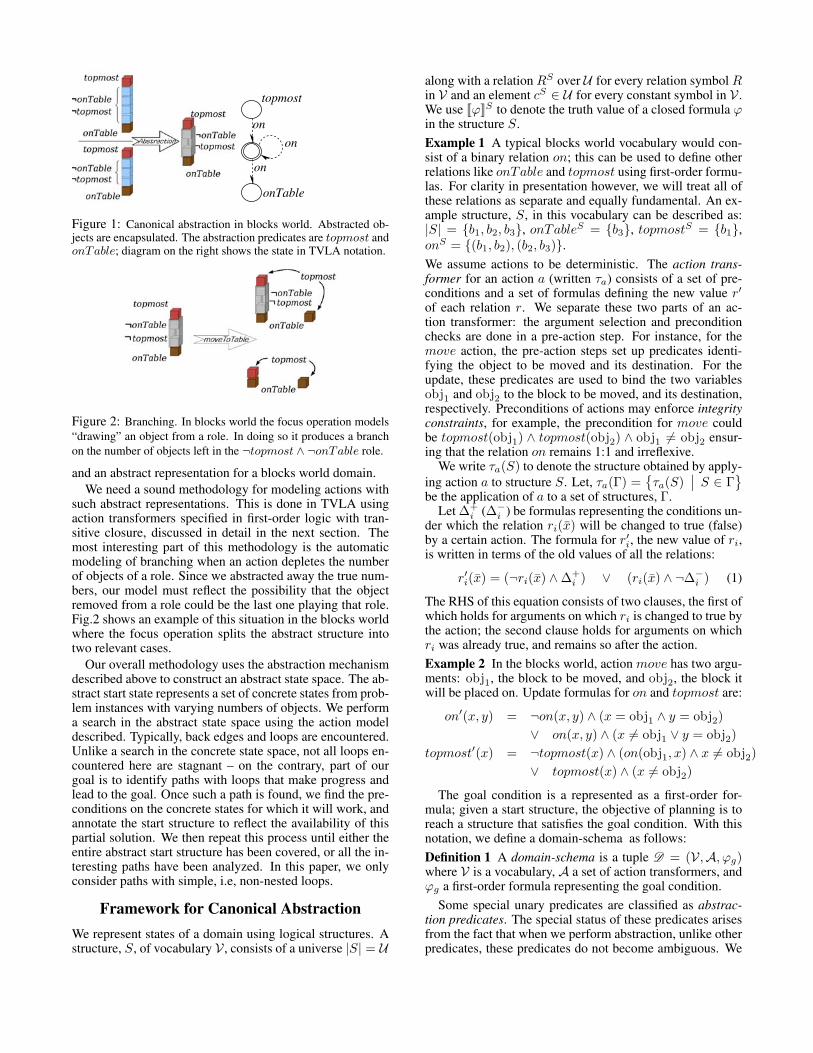
Figure 2: Branching. In blocks world the focus operation models

“drawing” an object from a role. In doing so it produces a branch

on the number of objects left in the ¬topmost ∧ ¬onTable role.

and an abstract representation for a blocks world domain.

We need a sound methodology for modeling actions withsuch abstract representations. This is done in TVLA usingaction transformers specified in first-order logic with tran-sitive closure, discussed in detail in the next section. Themost interesting part of this methodology is the automaticmodeling of branching when an action depletes the numberof objects of a role. Since we abstracted away the true num-bers, our model must reflect the possibility that the objectremoved from a role could be the last one playing that role.Fig.2 shows an example of this situation in the blocks worldwhere the focus operation splits the abstract structure intotwo relevant cases.

Our overall methodology uses the abstraction mechanismdescribed above to construct an abstract state space. The ab-stract start state represents a set of concrete states from prob-lem instances with varying numbers of objects. We performa search in the abstract state space using the action modeldescribed. Typically, back edges and loops are encountered.Unlike a search in the concrete state space, not all loops en-countered here are stagnant – on the contrary, part of ourgoal is to identify paths with loops that make progress andlead to the goal. Once such a path is found, we find the pre-conditions on the concrete states for which it will work, andannotate the start structure to reflect the availability of thispartial solution. We then repeat this process until either theentire abstract start structure has been covered, or all the in-teresting paths have been analyzed. In this paper, we onlyconsider paths with simple, i.e, non-nested loops.

Framework for Canonical AbstractionWe represent states of a domain using logical structures. Astructure, S, of vocabulary V , consists of a universe |S| = U

along with a relation RS over U for every relation symbol Rin V and an element cS ∈ U for every constant symbol in V .We use �ϕ�S to denote the truth value of a closed formula ϕin the structure S.

Example 1 A typical blocks world vocabulary would con-sist of a binary relation on; this can be used to define otherrelations like onTable and topmost using first-order formu-las. For clarity in presentation however, we will treat all ofthese relations as separate and equally fundamental. An ex-ample structure, S, in this vocabulary can be described as:|S| = {b1, b2, b3}, onTableS = {b3}, topmostS = {b1},

onS = {(b1, b2), (b2, b3)}.

We assume actions to be deterministic. The action trans-former for an action a (written τa) consists of a set of pre-conditions and a set of formulas defining the new value r′of each relation r. We separate these two parts of an ac-tion transformer: the argument selection and preconditionchecks are done in a pre-action step. For instance, for themove action, the pre-action steps set up predicates identi-fying the object to be moved and its destination. For theupdate, these predicates are used to bind the two variablesobj1 and obj2 to the block to be moved, and its destination,respectively. Preconditions of actions may enforce integrityconstraints, for example, the precondition for move couldbe topmost(obj1) ∧ topmost(obj2) ∧ obj1 �= obj2 ensur-ing that the relation on remains 1:1 and irreflexive.

We write τa(S) to denote the structure obtained by apply-

ing action a to structure S. Let, τa(Γ) ={τa(S)

∣∣ S ∈ Γ}

be the application of a to a set of structures, Γ.Let ∆+

i (∆−i ) be formulas representing the conditions un-

der which the relation ri(x̄) will be changed to true (false)by a certain action. The formula for r′i, the new value of ri,is written in terms of the old values of all the relations:

r′i(x̄) = (¬ri(x̄) ∧ ∆+i ) ∨ (ri(x̄) ∧ ¬∆−

i ) (1)

The RHS of this equation consists of two clauses, the first ofwhich holds for arguments on which ri is changed to true bythe action; the second clause holds for arguments on whichri was already true, and remains so after the action.

Example 2 In the blocks world, action move has two argu-ments: obj1, the block to be moved, and obj2, the block itwill be placed on. Update formulas for on and topmost are:

on′(x, y) = ¬on(x, y) ∧ (x = obj1 ∧ y = obj2)∨ on(x, y) ∧ (x �= obj1 ∨ y = obj2)

topmost′(x) = ¬topmost(x) ∧ (on(obj1, x) ∧ x �= obj2)∨ topmost(x) ∧ (x �= obj2)

The goal condition is a represented as a first-order for-mula; given a start structure, the objective of planning is toreach a structure that satisfies the goal condition. With thisnotation, we define a domain-schema as follows:

Definition 1 A domain-schema is a tuple D = (V,A, ϕg)where V is a vocabulary, A a set of action transformers, andϕg a first-order formula representing the goal condition.

Some special unary predicates are classified as abstrac-tion predicates. The special status of these predicates arisesfrom the fact that when we perform abstraction, unlike otherpredicates, these predicates do not become ambiguous. We

define the role an element plays as the set of abstractionpredicates it satisfies:

Definition 2 A role is a conjunction of literals consisting ofeach abstraction predicate or its negation.

Example 3 In the blocks world, with abstraction predicatestopmost and onTable, the role ¬topmost∧¬onTable des-ignates blocks that are in the middle of a stack.

Canonical AbstractionCanonical abstraction [Sagiv et al., 2002] groups states to-gether by only counting the number of elements of a roleup to two. If a role contains more than one element, theyare combined into a summary element. We can tune thechoice of abstraction predicates so that abstract structures ef-fectively model some interesting general planning problemsand yet the size and number of abstract structures remainsmanageable.

The imprecision that must result when states are merged ismodeled using three-value logic. In a three-valued structurethe possible truth values are 0, 1

2 , 1, where 12 means “don’t

know”. If we order these values as 0 < 12 < 1, then con-

junction evaluates to minimum, and disjunction evaluates tomaximum. See Fig.1 where on holds between the topmostblock, e1, and some but not all of the blocks of the summaryelement, e2. Thus the truth value of on(e1, e2) is 1

2 , drawnin TVLA as a dotted arc.

We next define embeddings [Sagiv et al., 2002]. De-fine the information order on the set of truth values as0 ≺ 1

2 , 1 ≺ 12 , so lower values are more precise. Intuitively,

S1 is embedabble in S2 if S2 is a correct but perhaps lessprecise representation of S1. In the embedding, several ele-ments of S1 may be mapped to a single summary element inS2.

Definition 3 Let S1 and S2 be two structures and f :|S1| → |S2| be a surjective function. f is an embeddingfrom S1 to S2 (S1 �f S2) iff for all relation symbols p of ar-ity k and elements, u1, . . . , uk ∈ |S1|, �p(u1, . . . , uk)�S1 ≺�p(f(u1), . . . , f(uk))�S2 .

The universe of the canonical abstraction, S′, of structure,S, is the set of nonempty roles of S:

Definition 4 The embedding of S into its canonical ab-straction wrt the set A of abstraction predicates is the map:

c(u) = e{p∈A|�p(x)�S,u/x=1},{p∈A|�p(x)�S,u/x=0}

Further, for any relation r, we have �r(e1, . . . , ek)�S′

=l.u.b�{�r(u1, . . . , uk)�S |c(u1) = e1, . . . , c(uk) = ek}.

Note that the subscript {p ∈ A|�p(x)�S,u/x = 1}, {p ∈A|�p(x)�S,u/x = 0} captures the role of the element u in S.Thus canonical abstraction merges all elements that have thesame role, see Fig.1. The truth values in canonical abstrac-tions are as precise as possible: if all embedded elementshave the same truth value then this truth value is preserved,otherwise we must use 1

2 . The set of concrete structures thatcan be embedded in an abstract structure S is called the con-cretization of S: γ(S) = {S′|∃f : S′ �f S}.

fψ Rolei RoleiRolei RoleiRolei

φφφ

S SS1 2 3S0

Figure 3: Effect of focus with respect to ϕ.

Focus With such an abstraction, the update formulas foractions might evaluate to 1

2 . We therefore need an effectivemethod for applying action transformers while not losing toomuch precision. This is handled in TVLA using the focusoperation. The focus operation on a three-valued structureS with respect to a formula ϕ produces a set of structureswhich have definite truth values for every possible instanti-ation of variables in ϕ, while collectively representing thesame set of concrete structures, γ(S). A focus operationwith a formula with one free variable is illustrated in Fig.3:if φ() evaluates to 1

2 on a summary element, e, then eitherall of e statisfies φ, or part of it does and part of it doesn’t,or none of it does. This process could produce structuresthat are inherently infeasible. Such structures are either re-fined or discarded using a set of restricted first-order for-mulas called integrity constraints. In Fig.3 for instance, ifintegrity constraints restricted φ to be unique and satisfiable,then structure S3 in Fig.3 would be discarded and the sum-mary elements for which φ() holds in S1 and S2 would bereplaced by singletons.

The focus operation wrt a set of formulas works by suc-cessive focusing wrt each formula in turn. The result ofthe focus operation on S wrt a set of formulas Φ is writ-ten fΦ(S). We use ψa to denote the set of focus formulasfor action a.

Choosing Action ArgumentsUsually, action specifications are allowed to have free vari-ables. During a typical TVLA execution, such an action istried with every binding of the free variables that satisfies thepre-conditions. In static analysis this feature can be used tomodel non-determinism. We choose the arguments in a se-ries of pre-action focus steps. For example, to choose obj1,in the move action we would focus on an auxiliary unarypredicate obj′1() that is constrained to be single-valued andto imply topmost.

Action ApplicationRecall that the predicate update formulas for action trans-former take the form shown in equation 1. This equationmight evaluate to indefinite truth values in abstract struc-tures. For our purposes, the most important updates are forabstraction predicates since precision in their values deter-mines the accuracy of modeling action dynamics. In thisspecial case, the expressions for ∆+

i and ∆−i are monadic

(i.e. have only one free variable apart from the action argu-ments which are bound by the pre-action steps).

In order to obtain definite truth values for these updates,we focus the given abstract structure S on the expressions∆±i . Once the action transformer has been applied, we again

apply canonical abstraction (this is called “blur” in TVLA)on the resulting structures to get the abstract result struc-tures.

Input: S0, D = (A, ϕg)

S ← S01while S � ϕg do

Nondeterministically execute action a ∈ A on S to get S′2S ← S′3

endAlgorithm 1: NDPlan

TransitionsOnce the action arguments have been chosen, there are threesteps involved in action application: action specific focus,

action transformation, and blur. The transition relationa−→

for each action a, captures the combined effect of these threesteps. More precisely,

Definition 5 (Transition Relation) S1a−→ S2 iff S1 and S2

are three-valued structures and there exists a focused struc-ture S1

1 ∈ fψa(S1) s.t. S2 = blur(τa(S11)).

Sometimes however we will need to study the exact path

S1 took in getting to S2. For this, the transition S1a−→ S2 can

be decomposed into a set of transition sequences {(S1fψa−−→

Si1τa−→ Si2

b−→ S2)|Si1 ∈ fψa(S1) ∧ Si2 = τa(Si1) ∧ S2 =blur(Si2)}.

TVLA can effectively generate the full instantiation ofthese transition relations for a given domain in the form of atransition graph, the subject of our next section.

Transition Graphs Transition graphs are graphs of all the

transition relationsa−→ with nodes representing structures.

Formally,

Definition 6 Given a domain D and an initial state S0, thetransition graph for D starting with S0, GD(S0) is the edge-

labeled multigraph defined by the set of relations { a−→: a ∈A} on the set of structures reachable from S0. Each edge ofGD(S0) is labeled by the appropriate action.

We omit the subscript D where it is understood from con-text. The entire transition graph of a domain, though finite,is usually an unwieldy structure. Its generation can be op-timized using various heuristics; owing to abstraction, thisin itself could be an interesting subject for research. In thispaper however, our focus is on using the transition graphrather than its efficient generation. The algorithm we pro-pose for generating plans allows for the dynamic generationof transition graphs; it can also be used in an on-line fashionby interleaving the search and transition graph generationphase with the analysis phase for iteratively obtaining par-tial solutions. We discuss this issue further in the Algorithmsection. For now, we present one very simple algorithm toshow that this graph can indeed be effectively generated.

Algorithm 1 shows NDPlan, a non-deterministic algo-rithm for finding plans. We use NDPlan as a program in-put to TVLA for generating G (S0). TVLA collects all thestructures that could possibly result from the execution ofa program statement at the next node in the program’s con-trol flow graph (CFG). Since the non-deterministic actionexecution could produce the effects of any of the actions inA, TVLA produces all of those structures at the CFG nodecorresponding to statement #3. Running TVLA on this plantherefore has the same effect as a BFS search for a goal state,

except that the search continues until all reachable structureshave been generated. In order to speed up this process, it ispossible to restrict its behavior so as to not explore actionson structures which are easily seen to be on the wrong track.

Our MethodologyThe idea behind our algorithm for generalized planning is tosuccessively find paths in a transition graph and for eachsuch path, to compute the pre-conditions under which ittakes concrete structures to structures satisfying the goal.

In order to accomplish this, we need a way of representingsubsets of abstract structures that are guaranteed to take aparticular branch of an action’s focus operation. Next, weneed to propagate these subsets backwards through actionedges in the given path all the way up to the start structure.

We represent subsets of an abstract structure by annotat-ing a structure with a set of conditions from a chosen con-straint language. In static analysis terms, we use annotationsto refine our abstraction. Formally,

Definition 7 (Annotated Structures) Let C be a languagefor expressing constraints on three-valued structures. AC−annotated structure S|C is a refinement of S consistingof structures in γ(S) that satisfy the condition C ∈ C. For-

mally, γ(S|C) ={s ∈ γ(S)

∣∣ s |= C}

.

We extend the notation defined above to sets of struc-tures, so that if Γ is a set of structures then by Γ|C we meanthe structures in Γ that satisfy C. Consequently, we haveγ(S|C) = γ(S)|C .

We now need to be able to identify the (annotated) pre-image of an annotated structure under any action. This re-quirement on a domain is captured by the following defini-tion:

Definition 8 (Annotated Domains) An annotated domain-schema is a pair 〈D , C〉 where D is a domain-schema andC is a constraint language. An annotated domain-schema is amenable to back-propagation if for every tran-

sition S1fψa−−→ Si1

τa−→ Si2b−→ S2 and C2 ∈ C there exists

Ci1 ∈ C such that τa(γ(S1)|Ci1) = τa(γ(Si1))|C2 .

In terms of this definition, since τa(γ(Si1)) is the subsetof γ(Si2) that has pre-images in Si1 under τa, S1|Ci1 is the

pre-image of S2|C2 under a particular focused branch (theone using Si1) of action a. The disjunction of Ci1 over allbranches taking S1 into S2 therefore gives us a more generalannotation which is not restricted to a particular branch ofthe action update. Therefore, we have:

Lemma 1 Suppose 〈D , C〉 is an annotated domain-schema that is amenable to back-propagation and S1, S2 ∈D such that S1

a−→ S2. Then for all C2 ∈ C there exists aC1 ∈ C such that τa(γ(S1)|C1) = (τa(γ(S1)) ∩ γ(S2))|C2 .

This lemma can be easily generalized through inductionto multi-step back-propagation along a sequence of actions.We use the abbreviation τk...1 to represent the successive ap-plication of action transformers a1 through ak, in this order.

Proposition 1 (Linear backup) Suppose 〈D , C〉 is an anno-tated domain-schema that is amenable to back-propagationand S1, . . . , Sk ∈ D are distinct structures such that S1

τ1−→

S2 · · · τk−1−−−→ Sk. Then for all Ck there exists C1 such thatτk−1...1(γ(S1)|C1) = τk−1...1(γ(S1)) ∩ Sk|Ck

The restriction of distinctness in this proposition confinesits application to action sequences without loops.

Amenability for back-propagation can be seen as beingcomposed of two different requirements. In terms of def-inition 8, we first need to translate the constraint C2 intoa constraint on Si1. Next, we need a constraint selecting thestructures in S1 that are actually in Si1. Composition of thesetwo constraints will give us the desired annotation, Ci1. Thesecond part of this annotation, classification, turns out to bea strong restriction on the focus operation. We formalize itas follows:

Definition 9 (Focus Classifiability) A focus operation fψ ona structure S satisfies focus classifiability with respect to aconstraint language C if for every Si ∈ fψ(S) there existsan annotation Ci ∈ C such that s ∈ γ(Si) iff s ∈ γ(S|Ci).

Since three-valued structures resulting from focus opera-tions with unary formulas are necessarily non-intersecting,we have that any s ∈ S may satisfy at most one of the con-ditionsCi. Focus classifiability is hard to achieve in general;we need it only for structures reachable from the start struc-ture.

Inequality-Annotated domain-schemas Let us denoteby #R(S) the number of elements of role R in structureS. In this paper, we use CI(R), the language consistingof constraints expressed as sets of linear inequalities using#Ri(S) for annotations. In order to make domain-schemasannotated with constraints in CI(R) amenable to back prop-agation, we first restrict the class of permissible actions tothose that change role counts by a fixed amount:

Definition 10 (Uniform Change) An action shows uniform

change w.r.t a set of roles R iff whenever S1fψa−−→ Si1

a−→Si2

b−→ S2 then ∀s1 ∈ γ(Si1), s2 ∈ γ(Si2) such that

s1a−→ s2, we have #Ri(s2) = g(#R1(s1), . . .#Rl(s1))

where g is a linear function determined by Si1 and Si2, andR1 . . . Rl ∈ R. In the special case where changes in thecounts of all roles are constants, we say the action showsconstant change.

The next theorem shows that uniform change gives usback-propagation if we already have focus-classifiability.

Theorem 1 (Back-propagation in inequality-annotated do-mains) An inequality-annotated domain-schema whose ac-tions show uniform change wrt R and focus operations sat-isfy focus classifiability wrt CI(R) is amenable to back prop-agation.

PROOF Suppose S1fψa−−→ Si1

a−→ Si2b−→ S2 and C2 is a set

of constraints on S2. We need to show that there exists a Ci1such that τa(γ(S1)|Ci1) = τa(γ(Si1))|C2 . Since we are given

focus-classifiability, we have Ci such that s ∈ γ(S1)|Ci iffs ∈ γ(Si1). We need to compose Ci with an annotation forreaching Si2|C2 to obtain Ci1. This can be done by rewrit-ing C2’s inequalities in terms of counts in S1 (counts don’tchange during the focus operation from S1 to Si1).

Suppose #Rj (Si2) = gj(#R1(S1), . . .#Rl(S1)). Then

we obtain the corresponding inequalities for S1 by substitut-

ing gj(#R1(S1), . . .#Rl(S1)) for #Rj (Si2) in all inequali-

ties ofC2. Naturally, if the resulting inequalities are satisfiedin S1,C2 will be satisfied in Si2. The resulting set of inequal-ities which we will callC1, gives us the rest of the desired in-equalities. The conjunction ofC1 andCi gives us the desiredannotation Ci1. That is, τa(γ(S1)|Ci1) = τa(γ(Si1)|C1) =τa(γ(Si1))|C2 . �

The next theorem provides a simple condition underwhich constant change holds.

Theorem 2 (Constant change) Let a be an action whosepredicate update formulas take the form shown in Eq. 1. Ac-tion a shows constant change if for every abstraction pred-icate pi, all the expressions ∆+

i ,∆−i are at most uniquely

satisfiable.

PROOF Suppose S1fψa−−→ Si1

τa−→ Si2b−→ S2; s1 ∈ γ(Si1)

and s1τa−→ s2 ∈ γ(Si2).

For constant change we need to show that #Ri(s2) =#Ri(s1)+δ where δ is a constant. Recall that a role is a con-junction of abstraction predicates or their negations. Further,because the focus formula fψa consists of pairs of formu-

las ∆+i and ∆−

i for every abstraction predicate, and theseformulas are at most uniquely satisfiable, each abstractionpredicate changes on at most 1 element. The focused struc-ture Si1 shows exactly which elements undergo change, andthe roles that they leave or will enter.

Therefore, since s1 is embeddable in Si1 and embeddingsare surjective, the number of elements leaving or enteringa role in s1 is the number of those singletons which enteror leave it in Si1. Hence, this number is the same for everys1 ∈ γ(Si1), and is a constant determined by Si1 and thefocus formulas. �

Quality of Abstraction In order for us to be able to clas-sify the effects of focus operations, we need to impose somequality-restrictions on the abstraction. Our main require-ment is that the changes in abstraction predicates shouldbe characterized by roles: given a structure, an action canchange a certain abstraction predicate only for objects witha certain role. We formalize this property as follows: a for-mula ϕ(x) is said to be role-specific in S iff only objects ofa certain role can satisfy ϕ in S. That is, there exists a roleR such that for every s ∈ γ(S), if (s, [c/x]) |= ϕ(x) then(s, c/x) |= R(x).

We therefore want our abstraction to be rich enough tomake the action change formulas, ∆±

i , role-specific in ev-ery structure encountered. For example, in the blocks worldstate shown in Fig.2 the move action can only change thetopmost predicate for a block of the role ¬topmost ∧¬onTable, representing blocks in the middle of the stack.The design of a problem representation and in particular, thechoice of abstraction predicates therefore needs to carefullybalance the competing needs of tractability in the transitiongraph and the precision required for back propagation.

The following proposition formalizes this in the form ofsufficient conditions for focus-classifiability. Note that fo-cus classifiability holds vacuously if the result of the focusoperation is a single structure (e.g., when the focus formulais unsatisfiable in all s ∈ γ(S), thus resulting in just onestructure with the formula false for every element).

Proposition 2 If ψ is unique, satisfiable in all s ∈ γ(S) andlocally role-specific for S then the focus operation fψ on Ssatisfies focus classifiability w.r.t CI(R).

PROOF Since the focus formula must hold for exactly oneelement of a certain role, the only branching possible is thatcaused due to different numbers of elements (zero vs. oneor more) satisfying the role while not satisfying the focusformula (see Fig.3). The branch is thus classifiable on thebasis of the count of the number of elements in the role. �

Corollary 1 If Φ is a set of uniquely satisfiable and role-specific formulas for S such that any pair of formulas in Φis either exclusive or equivalent, then the focus operation fΦon S satisfies focus classifiability.

Therefore any domain-schema whose actions only re-quire the kind of focus formulas specified by the corollaryabove is amenable to back-propagation. Because of the sim-ilarity of such domain-schemas with linked-lists, we callthem extended-LL domains:

Definition 11 (Extended-LL domains) An Extended-LL do-main with start structure Sstart is a domain-schema suchthat ∆+

i and ∆−i are role-specific, exclusive when not equiv-

alent, and uniquely satisfiable in every structure reach-able from Sstart. More formally, if Sstart →∗ S then∀i, j,∀e, e′ ∈ {+,−} we have ∆e

i role-specific and either

∆ei ≡ ∆e′

j or ∆ei =⇒ ¬∆e′

j in S.

Corollary 2 Extended-LL Domains are amenable to back-propagation.

Intuitively, these domain-schemas are those where:

1. The information captured by roles is sufficient to deter-mine whether or not an object of any role will undergochange due to an action; and

2. The number of objects being acquired or relinquished byany role is fixed (constant) for each action.

Examples of such domains are linked lists, blocks-worldscenarios (the appropriate start structures are defined in thesection on Examples), assembly domains where differentobjects can be constructed from constituent objects of dif-ferent roles etc.

Handling Paths with LoopsSo far we dealt exclusively with propagating annotationsback through a linear sequence of actions. In this section weshow that in extended-LL domains we can effectively prop-agate annotations back through paths consisting of simple(non-nested) loops.

Let us consider the path from S to Sf including the loop inFig.4; analysis of other paths including the loop is similar.The following proposition formalizes back-propagation inloops:

Proposition 3 (Back-propagation through loops) SupposeS0

τ1−→ S1τ2−→ . . .

τn−1−−−→ Sn−1τ0−→ S0 is a loop in an

extended-LL domain with a start structure Sstart. Let theloop’s entry and exit structures be S and Sf (Fig.4). Wecan then compute an annotation C(l) on S which selects thestructures that will be in Sf |Cf after l iterations of the loopon S, plus the simple path from S to Sf .

si 0s s’f

si+1sn−1

sf

ai+1

s’ a’i+1

ai

a0

a’1

an−1s

Figure 4: Paths with a simple loop. Outlined nodes represent

structures and filled nodes represent actions.

PROOF Our task is to find an annotation for the structureS which allows us to reach Sf |Cf , where Cf is a givenannotation. Since we are in an extended-LL domain, ev-ery action satisfies constant change. Let the individualchanges due to action ai on role count #Rj (S) be denoted

as δij . In general, this change depends on the structure onwhich the action is applied and the exact focused branchtaken. For clarity in presentation we omit these dependen-cies in the notation and assume different indices correspondto different actions. We use additional notation when deal-ing with action a0: its two branches are characterized by

changes δ0j and δ0fj . Our convention will be to add δij to

role #Rj (S) to obtain the count in τi(S), and subtract δijfrom a structure to find the role count before action appli-cation. As discussed in Theorem 1, the pre-image of anannotation C under action a can be obtained by replacingroles in every inequality in C in terms of their counterpartsbefore the action execution. In other words, we can writeτ−1i (C) = [#Rj (τi(S)) + δij/#Rj (S)]C.

We need to start going back from Sf and obtain expres-sions for annotations of every structure in the loop after lunwindings of the loop. Let us denote the annotation atstructure Sj during the lth unwinding of the loop to beCj(l). Cn−1(1) for Sn−1 in Fig.4 is therefore calculated

as τ−10 (Cf )

∧Cn−1→f , where Cn−1→f denotes the focus-

classification conditions required for taking the Sn−1 → Sfbranch of action a0.

In general these annotations can be defined inductively asfollows:

Ci(l) = τ−1i+1(Ci+1(l)) ∧ Ci→i+1 if i < n− 1

Cn−1(l) = τ−10 (C0(l − 1)) ∧ Cn−1→0 if l > 1

Cn−1(1) = τ−10f

(Cf ) ∧ Cn−1→f

Here, we distinguish between τ−10 and τ−1

0f: the former

represents the Sn−1 → S0 branch of a0; the latter theSn−1 → Sf branch.

In the rest of this discussion, we use τ−1n1..n2

as an abbrevi-

ation for τ−1n1

· τ−1n1+1 · · · τ−1

n2. Expanding the inductive rules

once, we get:

Cn−2(1) = τ−1n−1 · τ−1

0f(Cf ) ∧ τ−1

n−1(Cn−1→f )

∧C(n−2)→n−1

τ−1n−1 distributes over the expression because the inverse op-

eration amounts to a linear substitution.

Continuing in this way, we get the following expression

for Cm(1) where m < n− 1:

Cm(1) = τ−1m+1..n−1 · τ−1

0f(Cf )

∧n−1∧

k=m+1

τ−1m+1..k(Ck→k+1) ∧ Cm→m+1

where the successor of n−1 is treated as 0f . The first term ofthis expression is the back-propagation of Cf . The secondterm is a conjunction of back-propagation of all the focusclassification conditions necessary for us to stay in the loopuntil Sf . In subsequent unwindings of the loop, we will needthe Sn−1 → S0 branch, and consequently we will treat thesuccessor of n− 1 as 0 (addition modulo n).

Writing the second term as Cmloop(1), denoting the loop

conditions for first unwinding of the loop, we get

Cm(1) = τ−1m+1..n−1 · τ−1

0f(Cf ) ∧ Cmloop(1)

Using the inductive definitions, and writing the transforma-

tion over the entire loop, τ−1n−1..0 (or τ−1

n−1..0f) as τ−1 (or

τ−1f ), we get the general expression for Cm(l), l > 1 as:

Cm(l) = τ−1m..0 · τ−1(l−2) · τ−1

f (Cf )∧ τ−1

m..0 · τ−1(l−2)(C1loop(1))

∧ τ−1m..0 · τ−1(l−3)(C1

loop(2))...

∧ τ−1m..0τ

−1(C1loop(l − 2))

∧ τ−1m..0(C

1loop(l − 1))

However, note that the loop conditions C1loop(i) for i > 1

are all the same! Even with this simplification, the annota-tion described above presents a potentially large set of con-ditions. However, since the conditions are linear inequalitiesand the changes in roles are monotone with respect to thenumber of times the inverse operation is performed, thereare essentially four conditions at any Sm for lth unwindingof the loop. These conditions ensure all the other condi-tions (representing intermediate numbers of loop unwind-ings) hold:

Cm(l) = τ−1m..0 · τ−1(l−2) · τ−1

f (Cf )∧ τ−1

m..0 · τ−1(l−2)(C1loop(1))

∧ τ−1m..0 · τ−1(l−3)(C1

loop)∧ τ−1

m..0(C1loop)

And finally, we have the conditions #Rj (S) ≥ 0 for all jfor any S. �

Algorithm for Generalized PlanningLet the annotated-domain-schema〈D , CI〉 be an extended-LL domain with a start structure S0. Algorithm 2 shows ouralgorithm for generalized planning. It proceeds in phasesof search and annotation on the transition graph. Duringthe search phase it finds a path π from the start structure tostructures satisfying the goal condition. The transition graphcould also be dynamically generated during this phase. Dur-ing the annotation phase, it finds the annotation on S0, Cπfor π as described in the previous section. The resulting al-

Input: G (S0), Sg = {S : S ∈ G (S0) and S |= ϕg}, �:order on paths in G (S0)

Output: Π = {〈C, π〉 : s ∈ γ(S|C)⇒ π(s) |= ϕg}Π← ∅1while ∨{C : 〈C, π〉 ∈ Π} = � and ∃π: path not checkeddo

π ← getNextSmallest(S0,Sg)2Cπ ← findPrecon(S0, π,Sg)3if ∨{C : 〈C, π〉 ∈ Π} ⇒ Cπ then4

Π← Π ∪ {〈Cπ, π〉}5end

endAlgorithm 2: GenPlan

gorithm can be implemented in an any-time fashion, by out-putting plans capturing more and more problem instances asnew paths are found in the transition graph.

Procedure getNextSmallest(S0,Sg) returns the nextsmallest path with simple loops between S0 and membersof Sg . Procedure findPrecon(S0, π) returns the conditionson S0 under which the path π takes structures to Sg , as dis-cussed in the previous section.

Together with the definition of extended-LL domains andpropositions 3 and 1 Algorithm 2 realizes the following the-orem:

Theorem 3 (Generalized planning for extended-LL do-mains) For an extended-LL domain with a start structureS0 it is possible to find plans πi and annotations Ci suchthat ∀s ∈ γ(S|Ci), πi takes s to the goal; further, fors ∈ γ(S) \ γ(S|∨iCi), the goal is not reachable via planswith only simple loops in the transition graph G (S0).

ExamplesIn this section we formulate a problem in the blocks worlddomain in our framework and show how our algorithm findsa generalized plan. The formulation for linked lists is similarand can be used to find generalized plans for problems likereversing a linked list of unknown length i.e., to synthesizesimple programs.

Striped Block TowerRepresentation Our example is set in the blocks worlddomain with red and blue blocks. Given a stack consist-ing of red blocks below and blue blocks above, the goal is toconstruct a stack with alternating red and blue blocks abovean assigned red, base block with a blue block on top.

Our vocabulary consists of the predicates

{t[on]2, on2, topmost1, onTable1, obj11, obj12, red1, blue1, base1},

where all the unary predicates are abstraction predicates.t[on] is the transitive closure of on, and is used in integrityconstraints for the coerce operation. The obj1, obj2 predi-cates are used to select action arguments before an action isapplied. There are two actions: move(), which places obj1on top of obj2 and moveToTable(), which moves obj1 tothe table.

With this set of abstraction predicates, ∆±i are not role

specific in states with two or more stacks (their bases getmerged in the abstraction and the block below a selectedtopmost block could be either a block on table or a middleblock, violating role-specificity). One solution is to changethe problem definition so as to have a fixed, finite amount

Figure 5: Initial structure for striped blocks world.

Figure 6: Generalized plan with three loops found from the tran-sition graph. Numbers represent structure IDs from the transitiongraph.

of space for stacks on the table. Blocks not on any stackare placed in an unbounded size bag (captured by predicatebag). This will give us an additional set of abstraction pred-icates, onStacki, holding for every block in the ith stack.This separates stacks in the abstraction and ensures role-specificity for all states reachable from the canonical ab-straction of any real state with a bounded number of stacksof unbounded size. For simplicty, we restrict to only onestack in this demonstration.

Input Our initial abstract structure represents all probleminstances with a single stack of unknown and unboundednumbers of red and blue blocks (at least two of each). Thered blocks are below the blue blocks. Fig.5 shows the ini-tial structure in TVLA notation - relations with truth values12 are shown using dotted edges and summary elements areshown using double circles. To prune the search space, weadd a new abstraction predicate,misplaced, and use the fol-lowing heuristic: a block is misplaced if it is on a block ofthe same color, or above a misplaced block; a block is onlyplaced on another if it does not get misplaced in the pro-cess. This does not effect our main result because using thisheuristic reduces the size of the transition graph but not thesize of the resulting plan.

Output Fig.6 shows the most interesting branch of the ob-tained plan. It consists of three loops: the first loop movesall blue blocks to the table; the second, the red blocks, andfinally, the last loop moves blue and red blocks alternatelyback on to the stack. Algorithmically, this plan can be writ-ten as shown in Fig.7. The loops in this 20 step plan makeit sufficient for infinite problem instances with unboundednumbers of blocks. In the next section, we compute the pre-cise pre-conditions for this plan. Part of these pre-conditionsis the interesting fact that for our goal to be reachable, thenumber of blue blocks has to be equal to the number of red

Figure 7: Plan from Fig.6 written out in text.

blocks in the initial structure.

Annotations

In this section we provide an illustration for back-propagation of annotations. We wish to find the pre-conditions at structure 1 for true, or no annotation at Goal.Let Bt(Rt) be the roles corresponding to blue(red, but notbase) blocks that are onTable and topmost. Similarly, letBm(Rm) be the roles of blue(red) blocks that are neithertopmost nor onTable. In these terms, the edge 221 →Goal, is taken if there is exactly one Bt block in 221. Sim-ilarly, we exit from the last loop via 196 → 218 if there isonly one Rt block in 196. This makes the annotation at 221as [Rt = 1, Bt = 1]. Unrolling this annotation through the

loop, we get the the annotations for 196 after l unwindingsas: [Bt(196) = l+ 1, Rt(196) = l+ 1]. If l > 0, these con-

ditions subsume the conditions required for staying in theloop, which are Bt > 1 and Rt > 1. Continuing in this wayback through the other actions and loops and representingthe number of unwindings of “move red to table” (“moveblue to table”) as lr(lb), we get the annotation at structure 1as [Bt = l− lb, Rt = l− lr−1, Bm = 3+ lb, Rm = 4+ lr].

These conditions form the required pre-condition for thegiven plan to work. Together they imply that the total num-ber of blue blocks, #Bt + #Bm + 1 (+1 for the topmostblock in the initial structure) is 4 + l, exactly equal to thenumber of red blocks in the initial structure. If we also tallyrole counts with structures rather than simply propagatingthem backwards, we obtain the equalities l − lb = 0 andl − lr − 1 = 0 at structure 1. This tells us that number ofiterations of the stacking loop is equal to the number of it-erations of the unstack-blue-block loop; and further that weneeded to unstack one red block less (the base).

Cases with fewer number of blocks are captured by otherpaths (found before this path), and their pre-conditions areobtained similarly. Our algorithm thus finds a generalizedplan for solving infinitely many instances of the given ab-stract problem. In this case in fact, we get a solution for allsolvable instances. The stacking loop in this example alsodemonstrates that in comparison to DISTILL, our techniquesdo not impose any a-priori restrictions on the number of ac-tions in a loop.

Input: π = (a1, . . . , an): plan for S#0 ; S#

i = ai(S#i−1)

Output: Generalized plan ΠS0 ← c(S#); Π← π; CΠ ← �1Apply transformers for π on S0 to get S′

i−1, Si s.t.2

S′i−1 ∈ fai(Si−1), τi(S

′i−1) = Si and S#

i � Si.if ∃C ∈ CI(R) : Sn|C |= ϕg then3

Π← formLoops(S0 : a1 . . . , Sn−1 : an, Sn)4CΠ ← findPrecon(S0, Π, ϕg)5

endreturn Π, CΠ6

Algorithm 3: GeneralizeExample

Generalizing from ExamplesIn this section we present a simple application of our frame-work for computing a generalized plan from a plan thatworks for a single problem instance. The idea behind thistechnique is that if a given concrete plan contains sufficientunrollings of some simple loops, then we can automaticallyidentify these loops by observing the plan on a suitable ab-stract structure. We can then enhance this plan using theidentified loops and use the techniques discussed in this pa-per to find the set of problem instances for which this newgeneralized plan will work. The procedure is shown in Al-gorithm 3.

Given a concrete example plan π for S#0 , we start with an

abstract structure S0 for the start state. S0 can be any ab-stract structure which makes the resulting domain extended-LL, and for which we wish to find the restriction underwhich a generalization of π will work; the canonical abstrac-

tion of S#0 forms a natural choice. If the final abstract struc-

ture Sn or its restriction satisfies the goal, we have a generalplan and we proceed to find its pre-conditions.

The formLoops subroutine converts a linear path ofstructures and actions into a path with simple loops. Oneway of implementing this routine is by making a single passover the input path, and adding back edges whenever a struc-ture Sj is found such that Si = Sj(i < j), and Si is notpart of, or behind a loop. Structures and actions followingSj are merged with those following Si if they are identi-cal; otherwise, the loop is exited via the last action edge.This method produces one of the possibly many simple-loop paths from π; we could also produce all such paths.formLoops thus gives us a generalization Π of π. We thenuse the findPrecons subroutine to obtain the restriction onS0 for which Π works.

ExampleWe illustrate this idea using the blocks world setting fromthe previous section. Let us call the generalized plan shownin Fig.6 ΠG. Suppose we are given a concrete version

π = a1, . . . , an of ΠG for the initial structure S#0 corre-

sponding to a stack with 5 blue blocks above 5 red blocks.π would have 9 moveToTable actions followed by 9 ac-tions alternately moving red and blue blocks to the stack.π could have been generated by any classical planner. Let

S#i = ai(S

#i−1), i > 0.

To obtain the general plan, we first convert π into a se-quence of action transformers by replacing each action witha transformer that uses as its argument(s) any block havingthe role of the real action’s argument(s) (focus-based choice

operations described earlier could be used to do so). We thenapply the resulting sequence of transformers to the canonical

abstraction of S#0 (Fig.5). This gives us a sequence of sets

of structures representing the possibilities after each action.From each set in the sequence, we select the structure Sisuch that S#

i � Si. Note that πabs has the same start state,and action transformers as ΠG. Further, because of abstrac-tion its structure and action sequence is an unrolled versionof ΠG’s and every unrolled loop in Πabs is punctuated by arepeated abstract structure.

When formLoops is executed on Πabs, it finds the re-peated structures and re-creates the loops, giving us exactlyΠG! Finally, since Sn satisfies the goal, we use the tech-niques presented in this paper to find the problem instancesfor which Π will work.

We are thus able to extract the generalized plan ΠG fromπ, a simple concrete plan that could have been found byany classical planner. This approach is particularly effectiveif the goal condition only uses abstraction predicates (e.g.∀x¬misplaced(x)).

Conclusion and Future WorkWe present a new framework for generalized planning usingabstraction across problem instances to conduct the searchfor generalized plans. The main contributions of the paperare the presentation of an abstraction technique particularlyconducive for this purpose, the formulation of the planningalgorithms, and a precise analytical characterization of thesettings in which they work. We also show how to use thisframework to learn a general plan from examples. Our plan-ning algorithm is only partially implemented; a full imple-mentation requires interfacing with TVLA and is left for fu-ture work. We use several examples to illustrate how the al-gorithm works and to demonstrate the overall power of thisapproach.

Our framework opens up several interesting research av-enues for future work. Searching in an abstract space thatspans different problem instances presents new challengesfor heuristic and pruning techniques. Generalizing our tech-niques to a wider class of domains and plans with nestedloops are natural extensions that are worth exploring. Fi-nally, other annotation languages could be examined as theymay provide a way of moving beyond extended-LL do-mains.

ReferencesCimatti, A.; Roveri, M.; and Traverso, P. 1998. Automatic OBDD-

Based Generation of Universal Plans in Non-Deterministic Do-mains. Proc. of AAAI-98.

Feng, Z., and Hansen, E. A. 2002. Symbolic Heuristic Search forfactored Markov Decision Processes. Proc. of AAAI-02

Fikes, R.; Hart, P.; and Nilsson, N. 1972. Learning and Execut-ing Generalized Robot Plans. Technical report, AI Center, SRIInternational.

Hammond, K. J. 1996. Chef: A Model of Case Based Planning.Proc. of AAAI-96

Hoey, J.; St-Aubin, R.; Hu, A.; and Boutilier, C. 1999. SPUDD:Stochastic planning using decision diagrams. Proc. of UAI-99

Kambhampati, S., and Kedar, S. 1993. A Unified Framework forExplanation-Based Generalization of Partially Ordered and Par-tially Instantiated Plans. Artificial Intelligence.

Knoblock, C. A. 1991. Search Reduction in Hierarchical ProblemSolving. Proc. of AAAI-91

Loginov, A.; Reps, T.; and Sagiv, M. 2006. Automated verificationof the Deutsch-Schorr-Waite tree-traversal algorithm. Proc. ofSAS-06

Sagiv, M.; Reps, T.; and Wilhelm, R. 2002. Parametric shapeanalysis via 3-valued logic. Proc. of TOPLAS-02.

Veloso, M. 1994. Planning and Learning by Analogical Reason-ing. Springer-Verlag.

Winner, E., and Veloso, M. 2002. Automatically acquiring plan-ning templates from example plans. Proc. of AIPS-02.

Winner, E., and Veloso, M. 2003. DISTILL: Learning domain-

specific planners by example. Proc. of ICML-03