Exploiting the information content of hydrological "outliers" for goodness-of-fit testing

HESSD7, 4851–4874, 2010

Exploiting theinformation content

of hydrologicaloutliers

F. Laio et al.

Title Page

Abstract Introduction

Conclusions References

Tables Figures

J I

J I

Back Close

Full Screen / Esc

Printer-friendly Version

Interactive Discussion

Discussion

Paper

|D

iscussionP

aper|

Discussion

Paper

|D

iscussionP

aper|

Hydrol. Earth Syst. Sci. Discuss., 7, 4851–4874, 2010www.hydrol-earth-syst-sci-discuss.net/7/4851/2010/doi:10.5194/hessd-7-4851-2010© Author(s) 2010. CC Attribution 3.0 License.

Hydrology andEarth System

SciencesDiscussions

This discussion paper is/has been under review for the journal Hydrology and EarthSystem Sciences (HESS). Please refer to the corresponding final paper in HESSif available.

Exploiting the information content ofhydrological “outliers” forgoodness-of-fit testingF. Laio, P. Allamano, and P. Claps

DITIC, Politecnico di Torino, Corso Duca degli Abruzzi 24, 10129 Torino, Italy

Received: 6 July 2010 – Accepted: 9 July 2010 – Published: 22 July 2010

Correspondence to: F. Laio ([email protected])

Published by Copernicus Publications on behalf of the European Geosciences Union.

4851

http://www.hydrol-earth-syst-sci-discuss.net

http://www.hydrol-earth-syst-sci-discuss.net/7/4851/2010/hessd-7-4851-2010-print.pdf

http://www.hydrol-earth-syst-sci-discuss.net/7/4851/2010/hessd-7-4851-2010-discussion.html

http://creativecommons.org/licenses/by/3.0/

HESSD7, 4851–4874, 2010



F. Laio et al.

Title Page



Tables Figures

J I

J I

Back Close

Full Screen / Esc



Discussion

Paper

|D

iscussionP

aper|

Discussion

Paper

|D

iscussionP

aper|

Abstract

Validation of probabilistic models based on goodness-of-fit tests is an essential step forthe frequency analysis of extreme events. The outcome of standard testing techniques,however, is mainly determined by the the behavior of the hypothetical model, FX (x), inthe central part of the distribution, while the behavior in the tails of the distribution,5

which is indeed very relevant in hydrological applications, is relatively unimportant forthe results of the tests. The maximum-value test, originally proposed as a techniquefor outlier detection, is a suitable, but seldom applied, technique that addresses thisproblem. The test is specifically targeted to verify if the maximum (or minimum) valuesin the sample are consistent with the hypothesis that the distribution FX (x) is the real10

parent distribution. The application of this test is hindered by the fact that the criticalvalues for the test should be numerically obtained when the parameters of FX (x) areestimated on the same sample used for verification, which is the standard situation inhydrological applications. We propose here a simple, analytically explicit, techniqueto suitably account for this effect, based on the application of censored L-moments15

estimators of the parameters. We demonstrate, with an application that uses artificiallygenerated samples, the superiority of this modified maximum-value test with respect tothe standard version of the test. We also show that the test has comparable or largerpower with respect to other goodness-of-fit tests (e.g., chi-squared test, Anderson-Darling test, Fung and Paul test), in particular when dealing with small samples (sample20

size lower than 20–25) and when the parent distribution is similar to the distributionbeing tested.

1 Introduction

An outlying observation, or outlier, is a record that appears to deviate markedly fromother members of the sample to which it belongs (Grubbs, 1969). It is clear from this25

definition that an outlier can occur either because data values are incorrect (e.g., dueto inaccurate recording or transcription), or because the population has an heavy-tailed

4852





HESSD7, 4851–4874, 2010



F. Laio et al.

Title Page



Tables Figures

J I

J I

Back Close

Full Screen / Esc



Discussion

Paper

|D

iscussionP

aper|

Discussion

Paper

|D

iscussionP

aper|

distribution, which increases the probability of having single observations which standway apart from the others (e.g., Barnett and Lewis, 1994). Still, the practitioners areoften tempted to omit the outliers from the available data samples, because this choiceallows one to proceed with the statistical analysis using simpler and well-behaved dis-tributions. While application of outlier detection methods may be extremely important5

for screening the data and recognizing gross errors, unsupervised outlier rejection mayresult in a remarkable loss of information, in particular when the behavior of the tails ofthe distribution is fundamental to the performed statistical analyses (which of course isexactly the case in the frequency analysis of hydrological extremes). To quote Gumbel(1960): “The rejection of outliers on a purely statistical basis is and remains a dan-10

gerous procedure. Its very existence may be a proof that the underlying population is,in reality, not what it was assumed to be”. In this paper we accept this viewpoint andshow how extreme observations, possibly marked as outliers, can be used to selectthe probabilistic model for the frequency analysis of extreme events.

This objective changes the statement of the problem, from one where the extreme15

observations are screened as potential outliers to be rejected, to one where they areused for validation of a probabilistic model, i.e., for goodness-of-fit purposes.

Several different testing techniques have been developed for application to the fre-quency analysis of hydrological extremes as, for example Vogel (1986), Ahmad et al.(1988), Chowdhury et al. (1991), Vogel and McMartin (1991), Fill and Stedinger (1995),20

Wang (1998) and Laio (2004). Alternatively, the model validation issue has been recastas a model selection problem, where several candidate models are compared, and thebest model to represent the available data is selected (e.g., Strupczewski et al., 2002;Mitosek et al., 2006; Di Baldassarre et al., 2008; Laio et al., 2009). However, a com-mon drawback of goodness-of-fit and model selection techniques is that their outcome25

is mainly determined by the behavior of the hypothetical model in the central part of thedistribution, while the behavior in the tails of the distribution, is relatively unimportantfor the outcome of the test: standard goodness-of-fit tests seldom reveal an ill-fittingtail without a very large amount of data (Bryson, 1974).

4853





HESSD7, 4851–4874, 2010



F. Laio et al.

Title Page



Tables Figures

J I

J I

Back Close

Full Screen / Esc



Discussion

Paper

|D

iscussionP

aper|

Discussion

Paper

|D

iscussionP

aper|

This problem can be overcome by using the maximum-value test, which was orig-inally proposed by Grubbs (1969) as a technique for outliers detection in a Gaus-sian setting, and subsequently extended to Gumbel-distributed parents by Rossi et al.(1984). The test is specifically targeted to verify if the maximum (or minimum) values inthe sample are consistent with the hypothesis that the distribution FX (x) corresponds5

to the real parent distribution. However, usual applications of this test to non-Gaussiandistributions are complicated by the fact that the parameters of the hypothetical dis-tribution, FX (x), are unknown and need to be estimated using the same sample usedfor the test, which in turn implies that the acceptance region for the test meeds to becalculated through numerical simulation (see e.g., Rossi et al., 1984).10

2 Methods

This section is devoted to describing the basic features of the maximum value test(Sect. 2.1), and of the necessary modifications to the testing procedure due to param-eter estimation on the same data sample used for testing (Sect. 2.2).

2.1 Basic definitions15

Suppose that x(1)≤...≤x(n) is an ordered sample of n independent observations from anunknown parent distribution with cumulative distribution function GX (x); also supposethat one wishes to test the null hypothesis that the data were sampled from a distribu-tion FX (x|Θ), where Θ is a vector of parameters that need to be estimated. In symbols,the null hypothesis to be tested is H0:GX (x)=FX (x|Θ). In this paper we will consider20

two- and three-parameter distributions as candidate operational models, i.e., as hy-pothetical parent distributions FX (x). More in detail, we will direct our attention to: (i)two-parameter distributions belonging to the location-scale family, i.e., distributions that

4854





HESSD7, 4851–4874, 2010



F. Laio et al.

Title Page



Tables Figures

J I

J I

Back Close

Full Screen / Esc



Discussion

Paper

|D

iscussionP

aper|

Discussion

Paper

|D

iscussionP

aper|

can be written in the form

F (x|θ1,θ2)=Φ(x−θ1

θ2

)(1)

where Φ(·) is a generic function, θ1 is a position (or location) parameter and θ2 isa scale parameter; (ii) three-parameter distributions belonging to the location-scale-shape family, characterized by the property5

F (x|θ1,θ2,θ3)=Φ(x−θ1

θ2;θ3

)(2)

where Φ(·;θ3) is a generic function with two arguments, the second argument beingthe shape parameter θ3. Most distribution commonly used in the hydrologic practicebelong to one of the two families indicated above, including the Gumbel distribution,the normal distribution, the two-parameter exponential distribution, the GEV distribu-10

tion, the Pearson type III (or three-parameter gamma) distribution, etc. (see Table 1 fordetails on the parametrization adopted in this paper). Other commonly used distribu-tions, as for example the lognormal, log-Pearson type III, and Frechet distributions, canbe traced back to these families with a preliminary log-transformation of the data.

Parameter estimation is here carried out with the L-moments method as defined, for15

example, in Hosking and Wallis (1997), because this method is especially suitable tobe used in combination with the maximum value test, as will be clarified in the following.The method of L-moments provides parameter estimators based on the matching ofdistribution and sample L-moments. The former are defined as

L1 =∫ 1

0x(u)du20

L2 =∫ 1

0(2u−1)x(u)du (3)

L3 =∫ 1

0(6u2−6u+1)x(u)du,

4855





HESSD7, 4851–4874, 2010



F. Laio et al.

Title Page



Tables Figures

J I

J I

Back Close

Full Screen / Esc



Discussion

Paper

|D

iscussionP

aper|

Discussion

Paper

|D

iscussionP

aper|

where x(u) is the quantile function of x, i.e., F (x(u))=u, 0<u<1. Unbiased estimatorsof sample L-moments are commonly written as

l1 =1n

n∑i=1

x(i )

l2 =1n

n∑i=1

(2(i −1)n−1

−1)x(i ) (4)

l3 =1n

n∑i=1

(6(i −1)(i −2)

(n−1)(n−2)−

6(i −1)

(n−1)+1)x(i ).5

Explicit relations for the estimation of distribution parameters are obtained for position-scale(-shape) distributions. In fact, for these distributions the quantile function can bewritten as

x(u)=θ1+θ2 ·z(u,θ3), (5)

where z(u,θ3) is the quantile function of the standardized variable z=(x−θ1)/θ2, which10

only depends on the probability level u and on the shape parameter θ3 (for two-parameter distributions of course the dependency on θ3 is lost). Using Eq. (5) in Eq. (3),distribution L-moments are re-written as

L1 =θ1+θ2

∫ 1

0z(u,θ3)du=θ1+θ2A(θ3)

L2 =θ2

∫ 1

0z(u,θ3)(2u−1)du=θ2B(θ3) (6)15

L3 =θ2

∫ 1

0z(u,θ3)(6u2−6u+1)du=θ2C(θ3),

4856





HESSD7, 4851–4874, 2010



F. Laio et al.

Title Page



Tables Figures

J I

J I

Back Close

Full Screen / Esc



Discussion

Paper

|D

iscussionP

aper|

Discussion

Paper

|D

iscussionP

aper|

where A(θ3), B(θ3) and C(θ3) are distribution dependent functions (or constant valuesin case of two-parameter distributions). For example, for the Gumbel distribution oneeasily obtains A=γE (where γE=0.5772... is the Euler constant) and B=ln(2) (the Cvalue is not required for two-parameter distributions). The values of A(θ3), B(θ3) andC(θ3) for the distributions considered in this paper are reported in Table 2.5

Estimators for location, scale, and shape parameters are now obtained by equating(Eqs. 4 and 6). Consequently, one obtains the following system of equations:

θ̂`1 = l1− θ̂`

2A(θ̂`

3

)θ̂`

2 = l2/B(θ̂`

3

)C(θ̂`

3

)B(θ̂`

3

) =l3l2.

(7)

These estimators are represented by using the superscript ` to denote that they arethe classical L-moments estimators, in order to avoid confusion with the modified es-10

timators introduced in the following subsection. The equations in the system can beseparately solved by starting from the bottom one, which allows one to find θ̂`

3 ; then

this result is used to find θ̂`2 from the central equation; finally θ̂`

2 and θ̂`3 are used in

the top equation to find θ̂`1 . In case of two-parameter distributions, only the first two

equations are needed, and the solution is analytically explicit.15

Once the parameters have been estimated, the maximum-value test can be applied.This test is specifically targeted to verify if the maximum (or minimum) values in thesample are consistent with the hypothesis that the distribution FX (x|Θ) is the real parentdistribution. In detail, the testing procedure requires that[FX (x(n)|Θ̂)

]n<1−α (8)20

4857





HESSD7, 4851–4874, 2010



F. Laio et al.

Title Page



Tables Figures

J I

J I

Back Close

Full Screen / Esc



Discussion

Paper

|D

iscussionP

aper|

Discussion

Paper

|D

iscussionP

aper|

where [FX (x|Θ̂)]n is the maximum value distribution (as defined, for example, by Kendalland Stuart (1979) and Kottegoda and Rosso (1998)), x(n) is the n-th order statistic (i.e.,the maximum value in the sample) and α is the significance level of the test. How-ever, usual applications of this test fail to consider the effects of parameter-estimation,i.e., of the substitution of Θ with Θ̂ in Eq. (8): when parameters are estimated for the5

same sample used for verification, the limiting values for the goodness-of-fit test (inthis case, 1−α) should be suitably recalculated, as explained in detail in D’Agostinoand Stephens (1986) and Laio (2004), among others. Here we follow a different ap-proach, as described in the following subsection, which allows one to suitably accountfor this effect, still maintaining the simplicity and full analytical tractability that are the10

distinctive features of the maximum value test.

2.2 Modified maximum-value test

In this section a simple and analytically explicit technique is proposed to account for theeffects of parameter estimation. Since the maximum-value test is based only on the n-th order statistic x(n), the basic idea is to avoid using x(n) in the parameter estimation, so15

that the test statistic will turn out to be completely independent of x(n). Of course it is notpossible to simply eliminate x(n) from the sample and carry out parameter estimationon the remaining n−1 values, because the resulting parameter estimators would besignificantly negatively biased. Therefore we explore the possibility to substitute x(n)with an estimator which is provided by the median of the hypothetical maximum value20

distribution,[FX (x̃(n)|Θ̂)

]n=0.5. (9)

Consequently, by considering Eqs. (9) and (5) one obtains

4858





HESSD7, 4851–4874, 2010



F. Laio et al.

Title Page



Tables Figures

J I

J I

Back Close

Full Screen / Esc



Discussion

Paper

|D

iscussionP

aper|

Discussion

Paper

|D

iscussionP

aper|

x̃(n) =θ1+θ2 ·z(

0.51/n,θ3

)=θ1+θ2 ·D(n,θ3), (10)

where D(n,θ3) is a distribution dependent function of the sample size n and shapeparameter θ3 (only of n in case of two-parameter distributions). For example, for theGumbel distribution D(n)=−ln[−ln[2]/n]. The values of D(n,θ3) for the other distribu-tions considered in this paper are reported in Table 2. New parameter estimators,5

independent of x(n) and therefore amenable for use in Eq. (8), can now be obtained byresorting to the substitution x̃(n)→x(n) in Eq. (4), and resolving the L-moments equa-tions to find out the new parameter estimators. More in detail, one can note that x(n)

always appears with a weight 1/n in the summations of Eq. (4), for L-moments ofany order. As a consequence, the substitution x̃(n)→x(n) trivially leads to the following10

modified form of sample L-moments estimators:

l ∗1 =1n

n−1∑i=1

xi +1nx̃(n) = l ′1+

1nx̃(n)

l ∗2 =1n

n−1∑i=1

(2(i −1)n−1

−1)xi +

1nx̃(n) = l ′2+

1nx̃(n)

l ∗3 =1n

n−1∑i=1

(6(i −1)(i −2)

(n−1)(n−2)−

6(i −1)

(n−1)+1)xi +

1nx̃(n)

= l ′3+1nx̃(n),

(11)

where l ′1, l ′2, and l ′3 are the first three sample L-moments calculated by excluding thelargest value in the sample, or l ′1=l1−x(n)/n, l ′2−x(n)/n, and l ′3−x(n)/n. By equating themodified sample L-moments in Eq. (11) to the distribution L-moments in Eq. (6) one15

4859





HESSD7, 4851–4874, 2010



F. Laio et al.

Title Page



Tables Figures

J I

J I

Back Close

Full Screen / Esc



Discussion

Paper

|D

iscussionP

aper|

Discussion

Paper

|D

iscussionP

aper|

obtains

θ̂1

(1− 1

n

)+ θ̂2

(A(θ̂3)−

D(n,θ̂3)

n

)= l ′1

−1nθ̂1+ θ̂2

(B(θ̂3)−

D(n,θ̂3)

n

)= l ′2

−1nθ̂1+ θ̂2

(C(θ̂3)−

D(n,θ̂3)

n

)= l ′3,

(12)

where Eq. (10) has also been used. The solution of the system of Eq. (12) allows oneto find out the modified estimators of the position, scale, and shape parameters, θ̂1,θ̂2, and θ̂3. We will denote these estimators as censored L-moments estimators of the5

distribution parameters, because the procedure of substitution of the maximum samplevalue resembles a Type 2 censoring.

By rearranging the term in Eq. (12) one obtains

B(θ̂3)−C(θ̂3)

B(θ̂3)(1− 1

n

)+ A(θ̂3)

n − D(n,θ̂3)n

=l ′2− l ′3

l ′2(1− 1

n

)+

l ′1n

, (13)

which can be used to find out the estimator of the shape parameter (by using the10

distribution-dependent functions defined in Table 2). This θ̂3 value can then be used in

θ̂2 =l ′2(1− 1

n

)+ 1

n l′1

B(θ̂3)(1− 1

n

)+ 1

nA(θ̂3)− D(n,θ̂3)n

, (14)

to find out the scale parameter estimator, θ̂2. As usual, for two-parameter distributionsEq. (14) can be directly used, without preliminary application of Eq. (13), because of

4860





HESSD7, 4851–4874, 2010



F. Laio et al.

Title Page



Tables Figures

J I

J I

Back Close

Full Screen / Esc



Discussion

Paper

|D

iscussionP

aper|

Discussion

Paper

|D

iscussionP

aper|

course no shape parameter exists in this case. For example, for the Gumbel distribu-tion, by using the functions in Table 2 in Eq. (14), one easily finds

θ̂2 =l ′2(1− 1

n

)+ 1

n l′1

ln[2](1− 1

n

)+ 1

nγE − ln[ln[2]/n]n

. (15)

Finally, the two estimators θ̂2 and θ̂3 can be used to estimate the location parameterthrough the relation5

θ̂1 = l ′1− l ′2− θ̂2[A(θ̂3)−B(θ̂3)], (16)

which specifies to

θ̂1 = l ′1− l ′2− θ̂2[γE − ln[2]] (17)

for the Gumbel distribution.Some comments can be useful at this point to better contextualize the obtained re-10

sults:

– The censored L-moments estimators (Eqs. 13, 14 and 16) are independent of thesample maximum value, and for this reason are amenable for use in the maximumvalue test.

– For two-parameter distributions the result is analytically explicit, while for three-15

parameter distributions it requires to numerically solve (Eq. 13), which, however,is a rather trivial task with computers. We also note that the level of complexityof censored L-moments estimators is exactly the same as that of the standardL-moments estimators, that again require the numerical solution of the third ofEq. (7) to perform parameter estimation for three-parameter distributions.20

– For n→∞ the censored L-moments estimators converge to the standard L-moments estimators, θ̂1→θ̂`

1 , θ̂2→θ̂`2 , and θ̂3→θ̂`

3 . This can be easily verifiedby considering that for n→∞ one recovers the third of Eq. (7) from Eq. (13), the

4861





HESSD7, 4851–4874, 2010



F. Laio et al.

Title Page



Tables Figures

J I

J I

Back Close

Full Screen / Esc



Discussion

Paper

|D

iscussionP

aper|

Discussion

Paper

|D

iscussionP

aper|

second of Eq. (7) from Eq. (14), and the first of Eq. (7) from Eq. (16). Therefore,asymptotically one finds l ′1→l1, l ′2→l2, and l ′3→l3.

– In a rather different context (trying to compensate for rainfall outliers in short timeseries) Hershfield (1961, 1965) developed a partially similar procedure to accountfor the effect of maximum value elimination on parameter estimation. However,5

his results are limited to the first two moments (the mean and the variance) andthey are not valid for any distribution as the ones we present (because they wereobtained from real rainfall data). Moreover, these results were provided only ina graphical form, even if Koutsoyiannis (2000, p. 22) (in Greek) provides them inclosed analytical form.10

– Sometimes systematic records of data can be integrated with additional data,derived from measurements of significant occasional events. When a numberof occasional additional measurements is available, one can merge them withthe systematic ones (e.g., Bayliss and Reed, 2001), producing a new time seriesof “equivalent” length m, where m is the number of years between the first and15

the last measurement of both the systematic and the occasional record, mergedtogether. The MV test can be easily applied also to these merged samples ofsystematic and non-systematic data, by simply substituting m for n in Eq. (8), andby using Wang (1990) estimators of sample L-moments instead of the standardestimators in Eq. (4). The possibility to be applied when non-systematic data are20

present is a unique feature of the MV test, not shared by other commonly usedtesting techniques.

3 Application

In this section we compare the power of the modified maximum-value test (referredto as MV test from here onwards) to the performances of other goodness-of-fit tests25

and outlier detection procedures. To this aim the parent distribution, GX (x), from which4862





HESSD7, 4851–4874, 2010



F. Laio et al.

Title Page



Tables Figures

J I

J I

Back Close

Full Screen / Esc



Discussion

Paper

|D

iscussionP

aper|

Discussion

Paper

|D

iscussionP

aper|

synthetic samples of independent observations will be generated, is supposed to beknown. The null hypothesis to be tested is H0:GX (x)=FX (x) with the Gumbel distributionas hypothetical distribution, i.e., FX (x)=GUM (see notation in Table 1). The power of thetests (i.e., the ability of the test to recognize that H0 is false) is analyzed under differentparametrization of GX (x). Particular attention is payed to the behavior of the tests5

when dealing with small samples. The cases GX (x)=GEV and of GX (x)=TCEV (Rossiet al., 1984) are treated in Sects. 3.1 and 3.2, respectively. The benchmark tests, inboth cases, are the classical Pearson test and the Anderson-Darling test (referred to,respectively, as CHI and AD test in the following of the paper), plus a specific test foroutliers detection (Fung and Paul, 1985), called Fung-Paul (FP) test in the following of10

the paper.The classical Pearson test falls in the category of the chi-squared type tests. The

testing procedure requires that the range of x is partitioned in classes; a convenientprocedure to avoid arbitrariness and maximize the power of the test entails the choiceof k equiprobable classes under the hypothesized distribution, with k=2n0.4 (Moore,15

1986). The test statistic for the case 0 (i.e., when the parameters of FX (x) are fullyspecified a priori) is the chi-squared distribution with k−1 degrees of freedom. Con-versely, when the distribution FX (x) is not completely known there is a partial recoveryof degrees of freedom of the chi-squared distribution with respect to the commonly rec-ommended value of k−1, with the consequence that the asymptotic distribution will lie20

somewhere between a chi-square distribution with k−p−1 and k−1 degrees of free-dom (e.g., Kendall and Stuart, 1979).

The Anderson-Darling test is based on the comparison between the hypothetical,FX (x), and empirical distribution function, Fn(x), i.e., a cumulative probability distribu-tion function that concentrates a probability 1/n at each of the n values in the sample.25

The discrepancy between the two distributions can be measured with quadratic statis-tics of the form

∫x[Fn(x)−FX (x)]2Ψ(x)dx, where Ψ(x) is a weighting function. When

Ψ(x)=[FX (x)(1−FX (x))]−1 one obtains the Anderson-Darling statistic, called A2, whichhas the property of assigning more weight to the tails of the distribution than to the

4863





HESSD7, 4851–4874, 2010



F. Laio et al.

Title Page



Tables Figures

J I

J I

Back Close

Full Screen / Esc



Discussion

Paper

|D

iscussionP

aper|

Discussion

Paper

|D

iscussionP

aper|

central part. Critical values and percentage points for the AD test for EV1, NORM,GAM and GEV distributions can be calculated following the procedure described byLaio (2004).

The outlier detection procedure proposed by Fung and Paul (1985) is intended fortesting the discordancy of one or more outliers in a Gumbel sample. The test statistic is5

expressed as T=(x(n)−x(n−k))/(x(n)−x(1)), where k=1,2,3 is the number of outliers. Thetabulated significance levels can be found also in Barnett and Lewis (1994), abridgedfrom Fung and Paul (1985). The test is recommended for sample sizes in the rangen=[5÷20].

3.1 Gumbel vs. GEV10

The power of the modified MV test to recognize as non-Gumbel a GEV-distributedsample is evaluated hereinafter. In rigorous terms this corresponds to assuming asparent a GEV distribution, while the distribution to be tested is an EV1. In detail, 10 000samples formed by n elements (with n=[20÷50]) are generated from a GEV distributionwith fixed parameters θ1=1, θ2=1, and variable θ3 values. Note that positive θ3 values15

correspond to positive skewness of the distribution; when θ3=0 the GEV reduces to anEV1 distribution. For each sample, the parameters of an EV1 distribution are estimatedaccording to Eqs. (17) and (15), which introduced in Eq. (10) give x̃(n). The MV teststatistic, as expressed in Eq. (8), can then be resolved by resorting to the substitutionx̃(n)→x(n).20

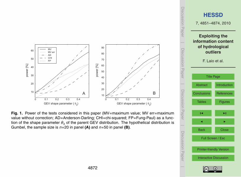
The results are reported in Fig. 1, by comparison with the FP, CHI and AD testperformances, at the 10% significance level. Also the case of the MV test applied withthe classical L-moments estimators (as in Eq. 7) is shown. Observe that the powerof the different tests converges to the significance level for null values of the shapeparameter, i.e., when the parent distribution collapses on a Gumbel. The left and right-25

hand side graphs are referred to the case of n=20 and n=50, respectively. One canobserve that, for rather small samples (e.g., n=20), which is a very common situation inhydrological applications, the MV test with censored parameters performs better than

4864





HESSD7, 4851–4874, 2010



F. Laio et al.

Title Page



Tables Figures

J I

J I

Back Close

Full Screen / Esc



Discussion

Paper

|D

iscussionP

aper|

Discussion

Paper

|D

iscussionP

aper|

the MV test with classical parameters estimates (which even fails to converge to thesignificance level when θ3=0). Also, the CHI test results to be by far less effective.By comparison to the FP test, the MV test turns out to be slightly more powerful. Asfor the AD test, the performances are comparable with a slight prevalence of the MVtest when the parent distribution is similar to the distribution considered in the null5

hypothesis (i.e., when θ3→0). The behavior is again similar, but more favorable to theAD test, for larger samples (as shown in the right panel of Fig. 1). The intersectionbetween the MV and AD curves, in fact, is shifted to the right, with smaller differencesbetween the test performances. This is due to the lesser influence of the maximumvalue in presence of larger samples, and is indicative of the MV test being more suited10

for application to small samples. Note that the comparison with the FP test is notpresent on the right-hand panel because Fung and Paul (1985) did not give the criticalvalues for n>20.

A possible explanation for the larger power of the MV test when θ3 is close to zero isprovided in Fig. 2. The design event xT is plotted as a function of return period T (i.e.,15

Eq. (5) is used with u=1−1/T ) for a GEV and a Gumbel distribution sharing the first twoL-moments. When θ3=0.15 (Fig. 2a) the two distributions are substantially overlappedup to a 20-year return period, and diverge only in the upper tail. In contrast, whenθ3=0.45 the two distributions are rather different also for low return periods (Fig. 2b).It is clear that the AD test, which is based on the comparison of the distributions in20

the whole probability range, will be favored in the latter situation, while the MV testwill perform better in situations like the one depicted in Fig. 2a, where the differencesconcentrate in the upper tail of the distributions. We note in passing that the abilityof the MV test to falsify the null hypothesis in these cases may be very important inpractical applications: for example, in the case of Fig. 2a, the wrong assumption of25

a Gumbel distribution would lead to a 30% underestimation of the 100-year designvalue.

4865





HESSD7, 4851–4874, 2010



F. Laio et al.

Title Page



Tables Figures

J I

J I

Back Close

Full Screen / Esc



Discussion

Paper

|D

iscussionP

aper|

Discussion

Paper

|D

iscussionP

aper|

3.2 Gumbel vs. TCEV

The MV test and AD test are compared also for the case when the parent distribution isa TCEV distribution (Rossi et al., 1984; Fiorentino et al., 1985) that is usually expressedin the form

GX (x)=exp[−exp

[−x−θ1

θ2

]−θ3 ·exp

[− 1θ4

x−θ1

θ2

]], (18)5

where θ1 is the position parameter, θ2 is the scale parameter, θ3 and θ4 are two shapeparameters. When θ3=0 the TCEV distribution reduces to a Gumbel distribution. A sig-nificance level α of 10% is again assumed for the tests. The CHI, FP, and non-modifiedMV tests are not considered in this example to facilitate the comparison between thetwo tests that performed better with a GEV parent distribution. The results are shown in10

Fig. 3, where the parameters of the “basic component” of a TCEV (to use the notationby Rossi et al., 1984 and Fiorentino et al., 1985) are kept constant (θ1=ln(10), θ2=1)while the parameters of the “outlying component” are allowed to vary. The three panelsrefer to different values of the parameter θ4, while the values of θ3 vary continuouslyon the x-axis. Only the case of n=20 is examined. In this case the MV test is found to15

be more powerful than the AD test for high θ4 values and low θ3 values; while the per-formances of both tests are poor for small θ4 values (panel C). Conversely, the AD testis more powerful for high θ3 values; in fact, the intersection of the two curves occursfor θ3'0.2 (panel A).

A similar behavior is therefore found with the two different parent distributions (GEV20

and TCEV): the MV test performs better than the AD test when the parent and hypo-thetical distributions are rather similar. A possible explanation of this behavior is thefollowing: when the discrepancies between the parent and hypothetical distribution arelarge, they significantly affect also the central part of the distribution, therefore increas-ing the discerning ability of standard testing techniques, as the AD test. In contrast,25

4866





HESSD7, 4851–4874, 2010



F. Laio et al.

Title Page



Tables Figures

J I

J I

Back Close

Full Screen / Esc



Discussion

Paper

|D

iscussionP

aper|

Discussion

Paper

|D

iscussionP

aper|

when the parent and hypothetical distribution are rather similar, one may spot the dif-ference only by looking at the tails of the distribution, i.e., for example, at the maximumobserved value.

4 Conclusions

Outliers in hydrological samples are often seen by the modelers as disturbing elements,5

because their very presence challenges well-established and convenient practices, bycontributing to raise doubts on the correctness of the hypothesized probability distri-bution model (for example, the adoption of the Gumbel distribution to represent floodor rainfall annual maxima). In this paper we follow the principle that, at least in somecases, it is exactly in the “outlying” data that resides very important information for10

the validation of the statistical model to be used in the frequency analysis of extremeevents. More in detail, we have described a procedure to perform a goodness-of-fittest based solely on the maximum recorded value in the sample. We have shown thatthe maximum value test represents a simple, analytically explicit, alternative to othercommonly used goodness-of-fit tests: this test performs consistently better than the15

Chi-squared test, and it proves to be more powerful than the Anderson-Darling test torecognize the lack of fit when the parent distribution is similar to the distribution beingtested. Since the test is based only on the maximum recorded value, it is particularlysuited when small samples (n≤20÷25) are available.

Acknowledgements. The work was funded by the Italian Ministry of Education (grants20

2007HBTS85 and 2008KXN4K8). We are grateful to D. Koutsoyiannis for providing the ref-erence to the works by Hershfield (1961, 1965) and for pointing us to his teaching material athttp://www.itia.ntua.gr/en/docinfo/116/.

4867





http://www.itia.ntua.gr/en/docinfo/116/

HESSD7, 4851–4874, 2010



F. Laio et al.

Title Page



Tables Figures

J I

J I

Back Close

Full Screen / Esc



Discussion

Paper

|D

iscussionP

aper|

Discussion

Paper

|D

iscussionP

aper|

References

Ahmad, M., Sinclair, C., and Spurr, B.: Assessment of flood frequency models using empiricaldistribution function statistics, Water Resour. Res., 24, 1323–1328, 1988. 4853

Barnett, V. and Lewis, T.: Outliers in Statistical Data, Springer Series in Statistics, John Wileyand Sons, 1994. 4853, 48645

Bayliss, A. and Reed, D.: The use of historical data in flood frequency estimation, Tech. rep.,Centre for Ecology and Hydrology, 2001. 4862

Bryson, M.: Heavy-tailed distributions: properties and tests, Technometrics, 16, 61–68, 1974.4853

Chowdhury, J., Stedinger, J., and Lu, L.: Goodness-of-fit tests for regional generalized extreme10

value flood distributions, Water Resour. Res., 27, 1765–1776, 1991. 4853D’Agostino, R. and Stephens, M.: Goodness-of-Fit Techniques, Marcel Dekker Inc, New York,

1986. 4858Di Baldassarre, G., Laio, F., and Montanari, A.: Design flood estimation using model selection

criteria, Phys. Chem. Earth, 34, 606–611, doi:10.1016/j.pce.2008.10.066, 2008. 485315

Fill, H. and Stedinger, J.: L-moment and probability plot correlation coefficient goodness-of-fit tests for the Gumbel distribution and impact of autocorrelation, Water Resour. Res., 31,225–229, 1995. 4853

Fiorentino, M., Versace, P., and Rossi, F.: Regional flood frequency estimation using the two-component extreme value distribution, Hydrolog. Sci. J., 30, 51–63, 1985. 486620

Fung, K. and Paul, S.: Comparison of outlier detection procedures in Weibull or Extreme-Valuedistribution, Commun. Stat. B.-Simul., 14, 895–917, 1985. 4863, 4864, 4865

Grubbs, F.: Procedures for detecting outlying observations in samples, Technometrics, 11, 1–21, 1969. 4852, 4854

Gumbel, E.: Discussion on rejection of outliers by Anscombe, F.J., Technometrics, 2, 165–166,25

1960. 4853Hershfield, D.: Estimating the probable maximum precipitation, J. Hydraul. Div., ASCE,

87(HY5), 99–106, 1961. 4862, 4867Hershfield, D.: Method for estimating probable maximum precipitation, J. Am. Water Works

Assoc., 57, 965–972, 1965. 4862, 486730

Hosking, J. and Wallis, J.: Regional Frequency Analysis: An Approach Based on L-Moments,Cambridge University Press, 1997. 4855, 4871

4868





HESSD7, 4851–4874, 2010



F. Laio et al.

Title Page



Tables Figures

J I

J I

Back Close

Full Screen / Esc



Discussion

Paper

|D

iscussionP

aper|

Discussion

Paper

|D

iscussionP

aper|

Kendall, M. and Stuart, A.: The Advanced Theory of Statistics, Charles Griffin and CompanyLimited, 1979. 4858, 4863

Kottegoda, N. and Rosso, R.: Statistics, Probability, and Reliability for Civil and EnvironmentalEngineers, McGraw-Hill, International Edition, 1998. 4858

Koutsoyiannis, D.: Probable maximum precipitation, available at: http://www.itia.ntua.gr/getfile/5

116/5/documents/2000HydrometPMP.pdf (last access: 16 July 2010), 2000 (in Greek). 4862Laio, F.: Cramer-von Mises and Anderson-Darling goodness of fit tests for extreme

value distributions with unknown parameters, Water Resour. Res., 40, W09308,doi:10.1029/2004WR003204, 2004. 4853, 4858, 4864

Laio, F., Di Baldassarre, G., and Montanari, A.: Model selection techniques for10

the frequency analysis of hydrological extremes, Water Resour. Res., 45, W07416,doi:10.1029/2007WR006666, 2009. 4853

Mitosek, H., Strupczewski, W., and Singh, V.: Three procedures for selection of annual floodpeak distribution, J. Hydrol., 323(1–4), 57–73, doi:10.1016/j.jhydrol.2005.08.016, 2006. 4853

Moore, D.: Tests of the chi-squared type, in: Goodness-of-Fit Techniques, Marcel Dekker, New15

York, 1986. 4863Rossi, F., Fiorentino, M., and Versace, P.: Two-component extreme value distribution for flood

frequency analysis, Water Resour. Res., 20, 847–856, 1984. 4854, 4863, 4866Strupczewski, W., Singh, V., and Weglarczyk, S.: Asymptotic bias estimation methods caused

by the assumption of false probability distributions, J. Hydrol., 258, 122–148, 2002. 485320

Vogel, R.: The probability plot correlation coefficient test for the normal, lognormal, and Gumbeldistributional hypotheses, Water Resour. Res., 22, 587–590, 1986. 4853

Vogel, R. and McMartin, D.: Probability plot goodness-of-fit and skewness estimation proce-dures for the Pearson type 3 distribution, Water Resour. Res., 27, 3149–3158, 1991. 4853

Wang, Q.: Unbiased estimation of probability weighted moments and partial probability25

weighted moments from systematic and historical flood information and their application toestimating the GEV distribution, J. Hydrol., 120, 115–124, 1990. 4862

Wang, Q.: Approximate goodness-of-fit tests of fitted generalized extreme value distributionsusing LH moments, Water Resour. Res., 34, 3497–3502, 1998. 4853

4869





http://www.itia.ntua.gr/getfile/116/5/documents/2000HydrometPMP.pdf



HESSD7, 4851–4874, 2010



F. Laio et al.

Title Page



Tables Figures

J I

J I

Back Close

Full Screen / Esc



Discussion

Paper

|D

iscussionP

aper|

Discussion

Paper

|D

iscussionP

aper|

Table 1. Probability models considered in this paper. Γ[·] is the gamma function.

Distribution Acronym CDF or PDF Range

Exponential EXP F (x,θ)=1−exp[−(x−θ1)/θ2

]θ1<x<∞

Gumbel or Extreme Value Type I EV1 F (x,θ)=exp[−exp

[−x−θ1

θ2

]]−∞<x<∞

Normal or Gaussian NORM f (x,θ)= 1√2πθ2

exp[− 1

2

(x−θ1

θ2

)2]

−∞<x<∞

Generalized Extreme Value GEV F (x,θ)=exp[−(

1+θ3(x−θ1)θ2

)−1/θ3]

θ3(θ1−x)θ2

<1

Gamma or Pearson Type 3 GAM f (x,θ)= 1|θ2 |Γ[θ3]

(x−θ1

θ2

)θ3−1exp[−x−θ1

θ2

]x−θ1

θ2>0

4870





HESSD7, 4851–4874, 2010



F. Laio et al.

Title Page



Tables Figures

J I

J I

Back Close

Full Screen / Esc



Discussion

Paper

|D

iscussionP

aper|

Discussion

Paper

|D

iscussionP

aper|

Table 2. Distribution dependent functions to be used for parameter estimation, as defined inEqs. (6) and (10). Γ[·] is the gamma function, Γ[·;·] is the incomplete gamma function, andNorminv is the inverse of the standardized Gaussian cumulative distribution function.

A(θ3) B(θ3) C(θ3) D(n,θ3)

EXP 1 0.5 – −ln[1−0.51/n]

EV1 γe ln[2] – −ln[ ln[2]n ]

NORM 0 1/√π – Norminv[0.51/n]

GEV Γ(1−θ3)−1θ3

(2θ3−1)Γ(1−θ3)θ3

(1+3θ3−2θ3 )Γ(1−θ3)θ3

(ln[2]n

)−θ3−1

θ3

GAM θ3Γ[θ3+1/2]

Γ[θ3]√π

Γ[θ3+1/2]

Γ[θ3]√π·τ3

∗ 0.51/n=Γ[θ3,D(n,θ3)]Γ[θ3]

∗∗

∗ τ3 is the L-coefficient of skewness of the distribution. It can be computed using Eqs. (A.86)and (A.88) in Hosking and Wallis (1997).∗∗ Equation to be solved numerically.

4871





HESSD7, 4851–4874, 2010



F. Laio et al.

Title Page



Tables Figures

J I

J I

Back Close

Full Screen / Esc



Discussion

Paper

|D

iscussionP

aper|

Discussion

Paper

|D

iscussionP

aper|

0 0.1 0.2 0.3 0.4

10

20

30

40

50

60

GEV shape parameter ( q3)

pow

er

[%]

0 0.1 0.2 0.3 0.4

10

20

30

40

50

60

70

80

90MV

MV err

AD

CHI

FP

GEV shape parameter ( q3)

pow

er

[%]

A B

Fig. 1. Power of the tests considered in this paper (MV=maximum value; MV err=maximum valuewithout correction; AD=Anderson-Darling; CHI=chi-squared; FP= Fung-Paul) as a function of the shapeparameter θ3 of the parent GEV distribution. The hypothetical distribution is Gumbel, the sample size isn = 20 in panel A and n = 50 in panel B.

20

Fig. 1. Power of the tests considered in this paper (MV=maximum value; MV err=maximumvalue without correction; AD=Anderson-Darling; CHI=chi-squared; FP=Fung-Paul) as a func-tion of the shape parameter θ3 of the parent GEV distribution. The hypothetical distribution isGumbel, the sample size is n=20 in panel (A) and n=50 in panel (B).

4872





HESSD7, 4851–4874, 2010



F. Laio et al.

Title Page



Tables Figures

J I

J I

Back Close

Full Screen / Esc



Discussion

Paper

|D

iscussionP

aper|

Discussion

Paper

|D

iscussionP

aper|

5 10 50 100 500

T @yearsD

0

2

4

6

8

10

12

xT

A

5 10 50 100 500

T @yearsD

0

2

4

6

8

10

12

xT

B

Fig. 2. Comparison of a GEV(dashed line) and a Gumbel (solid line) distribution function sharing thefirst two L-moments. The design event xT is plotted as a function of return period T (in logarithmicscale). The parameter values for the GEV are θ1 = 0, θ2 = 1, θ3 = 0.15 in panel A and θ1 = 0, θ2 = 1,θ3 = 0.45 in panel B. The parameters of the Gumbel distribution are found by matching the first twodistribution L-moments to those of the GEV distribution.

21

Fig. 2. Comparison of a GEV(dashed line) and a Gumbel (solid line) distribution functionsharing the first two L-moments. The design event xT is plotted as a function of return period T(in logarithmic scale). The parameter values for the GEV are θ1=0, θ2=1, θ3=0.15 in panel (A)and θ1=0, θ2=1, θ3=0.45 in panel (B). The parameters of the Gumbel distribution are found bymatching the first two distribution L-moments to those of the GEV distribution.

4873





HESSD7, 4851–4874, 2010



F. Laio et al.

Title Page



Tables Figures

J I

J I

Back Close

Full Screen / Esc



Discussion

Paper

|D

iscussionP

aper|

Discussion

Paper

|D

iscussionP

aper|

0.05 0.1 0.15 0.2 0.25 0.3

20

30

40

50

60

70

80

TCEV shape parameter ( )q

0.05 0.1 0.15 0.2 0.25

15

20

25

30

35

40

45

50

0.02 0.04 0.06 0.08 0.1 0.12

10

11

12

13

14

15

16

MVAD

A B

C

pow

er

[%]

3 TCEV shape parameter ( )q TCEV shape parameter ( )q3 3

Fig. 3. Power of the maximum value (MV) and Anderson-Darling (AD) test for a TCEV parent distribu-tion. In panel A θ4 = 10, in panel B θ4 = 5, and in panel C θ4 = 2. The sample size is n = 20.

22

Fig. 3. Power of the maximum value (MV) and Anderson-Darling (AD) test for a TCEV parentdistribution. In panel (A) θ4=10, in panel (B) θ4=5, and in panel (C) θ4=2. The sample size isn=20.

4874





Exploiting the information content of hydrological "outliers" for goodness-of-fit testing

Documents

Transcript of Exploiting the information content of hydrological "outliers" for goodness-of-fit testing