
Exploiting Functional Dependence in Query Optimization
334
Exploiting Functional Dependence in Query Optimization by Glenn Norman Paulley A thesis presented to the University of Waterloo in fulfilment of the thesis requirement for the degree of Doctor of Philosophy in Computer Science Waterloo, Ontario, Canada, 2000 c Glenn Norman Paulley 2000
-
Upload
khangminh22 -
Category
Documents
-
view
0 -
download
0
Transcript of Exploiting Functional Dependence in Query Optimization

Exploiting Functional Dependence
in Query Optimization
by
Glenn Norman Paulley
A thesis
presented to the University of Waterloo
in fulfilment of the
thesis requirement for the degree of
Doctor of Philosophy
in
Computer Science
Waterloo, Ontario, Canada, 2000
c© Glenn Norman Paulley 2000


I hereby declare that I am the sole author of this thesis.I authorize the University of Waterloo to lend this thesis to other institutions or in-
dividuals for the purpose of scholarly research.
I further authorize the University of Waterloo to reproduce this thesis by photocopy-ing or by other means, in total or in part, at the request of other institutions or individ-uals for the purpose of scholarly research.
iii


The University of Waterloo requires the signatures of all persons using or photocopy-ing this thesis. Please sign below, and give address and date.
v


Abstract
Functional dependency analysis can be applied to various problems in query optimiza-tion: selectivity estimation, estimation of (intermediate) result sizes, order optimization(in particular sort avoidance), cost estimation, and various problems in the area of se-mantic query optimization. Dependency analysis in an ansi sql relational model, how-ever, is made complex due to the existence of null values, three-valued logic, outer joins,and duplicate rows. In this thesis we define the notions of strict and lax functional depen-dencies, strict and lax equivalence constraints, and null constraints, which capture both alarge set of the constraints implied by ansi sql query expressions, including outer joins,and a useful set of declarative constraints for ansi sql base tables, including unique, ta-ble, and referential integrity constraints. We develop and prove a sound set of inferenceaxioms for this set of combined constraints, and formalize the set of constraints that holdin the result of each sql algebraic operator. We define an extended functional depen-dency graph model (fd-graph) to represent these constraints, and present and prove cor-rect a detailed polynomial-time algorithm to maintain this fd-graph for each algebraicoperator. We illustrate the utility of this analysis with examples and additional theoreti-cal results from two problem domains in query optimization: query rewrite optimizationsthat exploit uniqueness properties, and order optimization that exploits both functionaldependencies and attribute equivalence. We show that the theory behind these two ap-plications of dependency analysis is not only useful in relational database systems, butin non-relational database environments as well.
vii


Acknowledgements
For the last two weeks I have written scarcely anything. I have been idle. Ihave failed.
Katherine Mansfield, diary, 13 November 1921
Determination not to give in, and the sense of an impending shape keepone at it more than anything.
Virginia Woolf, diary, 11 May 1920
Thesis? What thesis?Motto of the uw Graduate House
Upon completing my Master’s degree in the spring of 1990, I applied to Waterloo topursue further study in information retrieval, hopefully with Frank Wm. Tompa. Andnow, nearly a decade later, I’ve completed a doctoral dissertation under Frank’s supervi-sion. However, as is clear from its title, this thesis has nothing to do with information re-trieval. Instead, Paul Larson took me on to study query optimization in an sql-to-imsgateway, which re-kindled my interest in database systems and provided the motivationfor much, if not all, of the work herein. After Paul left Waterloo for a career at MicrosoftResearch, I was paired with Frank. And good thing, too—I could not have hoped for twobetter mentors. I am indebted to both of them for their guidance, encouragement, andfriendship, and for giving me the tools with which to start a new career. I will greatly missthe regular opportunities we had to work together. I would also like to thank my exam-ining committee: Christoph Freytag, David Toman, Edward P. F. Chan, and Ajit Singh.Their comments on earlier drafts have been incorporated into the final text. My particu-lar thanks to Christoph, whose enthusiasm is as contagious as his advice is edifying.
During my tenure at Waterloo I had the privilege of working with several faculty, staff,and students who not only buoyed my spirits but inspired me to follow in their collec-tive footsteps. Ken Salem, Jo Atlee, Wm. Cowan, Darrell Raymond, Alfredo Viola, IgorBenko, Ian Bell, Gord Vreugdenhil, Dave Mason, Peter Buhr, Lauri Brown, David Clark,Andrej Brodnik, Naji Mouawad, Anne Pidduck, Gopi Krishna Attaluri, Martin Van Bom-mel, Weipeng Yan, Dexter Bradshaw, and Qiang Zhu all offered their friendship, encour-agement, ideas, and advice. I am grateful to them all, especially Darrell, who contributedmany useful comments to earlier drafts, and to Dave, who developed several of the com-plex LATEX macros used to typeset this thesis.
My colleagues and managers at Sybase, notably Dave Neudoerffer, Peter Bumbulis,Anil Goel, Mark Culp, Anisoara Nica, and Ivan Bowman, were a constant source of good
ix

ideas and encouragement. Dave never admonished me for taking too long. Without hissupport this thesis would have never been completed.
Funding for my studies came from several sources. Most important were scholar-ships awarded by the Information Technology Research Centre (now Communicationsand Information Technology Ontario, or cito), nserc, iode, and the Canadian Ad-vanced Technology Association (cata). Irene Mellick believed enough in me to arrangean unprecedented, private-sector three-year scholarship from the Great-West Life Assur-ance Company—with no strings attached. I sincerely thank all of these agencies for theirfinancial assistance.
I must also mention the contributions of two other individuals. Helen Tompa has beennothing short of a surrogate aunt to our twin boys, Andrew and Ryan, since they wereborn in April 1998. From trips to the doctor to swimming lessons, ‘Aunt’ Helen has al-ways been ready to lend a hand. Thank you, Helen!
Barb Stevens rn coached us through some difficult periods in the past five years. Ondifferent occasions Barb has played the roles of coach, counselor, and friend, and alwayswith a touch of laughter. Her contribution to the completion of this thesis is far fromsmall.
Finally, and most of all, I thank my wife Leslie for being there with me at every stepof this long adventure. Despite being displaced from her family, selling our home in Win-nipeg, changing employers, the drop (!) in income, the working vacations, and the all-too-numerous lonely evenings, she knew how important this was to me.
It wasn’t supposed to take nearly this long. But as our boys so often pronounce, withthe enthusiasm only a two-year-old can muster: “all done!”
gnp
14 April 2000
x

Dedication
for Leslie, Andrew, and Ryan
xi


Contents
1 Introduction 1
2 Preliminaries 7
2.1 Class of sql queries considered . . . . . . . . . . . . . . . . . . . . . . . . 72.2 Extended relational model . . . . . . . . . . . . . . . . . . . . . . . . . . . 92.3 An algebra for sql queries . . . . . . . . . . . . . . . . . . . . . . . . . . . 12
2.3.1 Query specifications . . . . . . . . . . . . . . . . . . . . . . . . . . 142.3.1.1 Select-project-join expressions . . . . . . . . . . . . . . . 142.3.1.2 Translation of complex predicates . . . . . . . . . . . . . 192.3.1.3 Outer joins . . . . . . . . . . . . . . . . . . . . . . . . . . 222.3.1.4 Grouping and aggregation . . . . . . . . . . . . . . . . . 24
2.3.2 Query expressions . . . . . . . . . . . . . . . . . . . . . . . . . . . 282.4 Functional dependencies as constraints . . . . . . . . . . . . . . . . . . . . 32
2.4.1 Constraints in ansi sql . . . . . . . . . . . . . . . . . . . . . . . . 322.5 sql and functional dependencies . . . . . . . . . . . . . . . . . . . . . . . 35
2.5.1 Lax functional dependencies . . . . . . . . . . . . . . . . . . . . . . 362.5.2 Axiom system for strict and lax dependencies . . . . . . . . . . . . 372.5.3 Previous work regarding weak dependencies . . . . . . . . . . . . . 39
2.5.3.1 Null values as unknown . . . . . . . . . . . . . . . . . . . 402.5.3.2 Null values as no information . . . . . . . . . . . . . . . . 42
2.6 Overview of query processing . . . . . . . . . . . . . . . . . . . . . . . . . 432.6.1 Internal representation . . . . . . . . . . . . . . . . . . . . . . . . . 442.6.2 Query rewrite optimization . . . . . . . . . . . . . . . . . . . . . . 47
2.6.2.1 Predicate inference and subsumption . . . . . . . . . . . 482.6.2.2 Algebraic transformations . . . . . . . . . . . . . . . . . . 51
2.6.3 Plan generation . . . . . . . . . . . . . . . . . . . . . . . . . . . . . 592.6.3.1 Physical properties of the storage model . . . . . . . . . . 61
2.6.4 Plan Selection . . . . . . . . . . . . . . . . . . . . . . . . . . . . . 622.6.5 Summary . . . . . . . . . . . . . . . . . . . . . . . . . . . . . . . . 63
xiii

3 Functional dependencies and query decomposition 65
3.1 Sources of dependency information . . . . . . . . . . . . . . . . . . . . . . 663.1.1 Axiom system for strict and lax dependencies . . . . . . . . . . . . 663.1.2 Primary keys and other table constraints . . . . . . . . . . . . . . 683.1.3 Equality conditions . . . . . . . . . . . . . . . . . . . . . . . . . . . 683.1.4 Scalar functions . . . . . . . . . . . . . . . . . . . . . . . . . . . . . 71
3.2 Dependencies implied by sql expressions . . . . . . . . . . . . . . . . . . 713.2.1 Base tables . . . . . . . . . . . . . . . . . . . . . . . . . . . . . . . 733.2.2 Projection . . . . . . . . . . . . . . . . . . . . . . . . . . . . . . . . 743.2.3 Cartesian product . . . . . . . . . . . . . . . . . . . . . . . . . . . 753.2.4 Restriction . . . . . . . . . . . . . . . . . . . . . . . . . . . . . . . 763.2.5 Intersection . . . . . . . . . . . . . . . . . . . . . . . . . . . . . . . 793.2.6 Union . . . . . . . . . . . . . . . . . . . . . . . . . . . . . . . . . . 813.2.7 Difference . . . . . . . . . . . . . . . . . . . . . . . . . . . . . . . . 823.2.8 Grouping and Aggregation . . . . . . . . . . . . . . . . . . . . . . 83
3.2.8.1 Partition . . . . . . . . . . . . . . . . . . . . . . . . . . . 833.2.8.2 Projection of a grouped table . . . . . . . . . . . . . . . . 84
3.2.9 Left outer join . . . . . . . . . . . . . . . . . . . . . . . . . . . . . 843.2.9.1 Input dependencies and left outer joins . . . . . . . . . . 853.2.9.2 Left outer join: On conditions . . . . . . . . . . . . . . . 89
3.2.10 Full outer join . . . . . . . . . . . . . . . . . . . . . . . . . . . . . 973.2.10.1 Input dependencies and full outer joins . . . . . . . . . . 993.2.10.2 Full outer join: On conditions . . . . . . . . . . . . . . . . 99
3.3 Graphical representation of functional dependencies . . . . . . . . . . . . 1023.3.1 Extensions to fd-graphs . . . . . . . . . . . . . . . . . . . . . . . . 104
3.3.1.1 Keys . . . . . . . . . . . . . . . . . . . . . . . . . . . . . 1053.3.1.2 Real and virtual attributes . . . . . . . . . . . . . . . . . 1063.3.1.3 Nullable attributes . . . . . . . . . . . . . . . . . . . . . . 1073.3.1.4 Equality conditions . . . . . . . . . . . . . . . . . . . . . 1073.3.1.5 Lax functional dependencies . . . . . . . . . . . . . . . . 1083.3.1.6 Lax equivalence constraints . . . . . . . . . . . . . . . . . 1093.3.1.7 Null constraints . . . . . . . . . . . . . . . . . . . . . . . 1103.3.1.8 Summary of fd-graph notation . . . . . . . . . . . . . . . 110
3.4 Modelling derived dependencies with fd-graphs . . . . . . . . . . . . . . . 1133.4.1 Base tables . . . . . . . . . . . . . . . . . . . . . . . . . . . . . . . 114
xiv

3.4.2 Handling derived attributes . . . . . . . . . . . . . . . . . . . . . . 116
3.4.3 Projection . . . . . . . . . . . . . . . . . . . . . . . . . . . . . . . . 118
3.4.4 Cartesian product . . . . . . . . . . . . . . . . . . . . . . . . . . . 121
3.4.5 Restriction . . . . . . . . . . . . . . . . . . . . . . . . . . . . . . . 123
3.4.6 Intersection . . . . . . . . . . . . . . . . . . . . . . . . . . . . . . . 128
3.4.7 Grouping and Aggregation . . . . . . . . . . . . . . . . . . . . . . 130
3.4.7.1 Partition . . . . . . . . . . . . . . . . . . . . . . . . . . . 131
3.4.7.2 Grouped table projection . . . . . . . . . . . . . . . . . . 133
3.4.8 Left outer join . . . . . . . . . . . . . . . . . . . . . . . . . . . . . 134
3.4.8.1 Algorithm . . . . . . . . . . . . . . . . . . . . . . . . . . 137
3.4.9 Full outer join . . . . . . . . . . . . . . . . . . . . . . . . . . . . . 141
3.4.10 Algorithm modifications to support outer joins . . . . . . . . . . . 142
3.5 Proof of correctness . . . . . . . . . . . . . . . . . . . . . . . . . . . . . . 143
3.5.1 Proof overview . . . . . . . . . . . . . . . . . . . . . . . . . . . . . 144
3.5.1.1 Assumptions for complexity analysis . . . . . . . . . . . . 147
3.5.1.2 Null constraints . . . . . . . . . . . . . . . . . . . . . . . 148
3.5.2 Basis . . . . . . . . . . . . . . . . . . . . . . . . . . . . . . . . . . . 149
3.5.3 Induction . . . . . . . . . . . . . . . . . . . . . . . . . . . . . . . . 151
3.5.3.1 Projection . . . . . . . . . . . . . . . . . . . . . . . . . . 152
3.5.3.2 Cartesian product . . . . . . . . . . . . . . . . . . . . . . 157
3.5.3.3 Restriction . . . . . . . . . . . . . . . . . . . . . . . . . . 159
3.5.3.4 Intersection . . . . . . . . . . . . . . . . . . . . . . . . . . 164
3.5.3.5 Partition . . . . . . . . . . . . . . . . . . . . . . . . . . . 167
3.5.3.6 Grouped table projection . . . . . . . . . . . . . . . . . . 168
3.5.3.7 Left outer join . . . . . . . . . . . . . . . . . . . . . . . . 168
3.6 Closure . . . . . . . . . . . . . . . . . . . . . . . . . . . . . . . . . . . . . 173
3.6.1 Chase procedure for strict and lax dependencies . . . . . . . . . . 175
3.6.2 Chase procedure for strict and lax equivalence constraints . . . . . 182
3.7 Related work . . . . . . . . . . . . . . . . . . . . . . . . . . . . . . . . . . 187
3.8 Concluding remarks . . . . . . . . . . . . . . . . . . . . . . . . . . . . . . 190
xv

4 Rewrite optimization with functional dependencies 193
4.1 Introduction . . . . . . . . . . . . . . . . . . . . . . . . . . . . . . . . . . . 1934.2 Formal analysis of duplicate elimination . . . . . . . . . . . . . . . . . . . 194
4.2.1 Main theorem . . . . . . . . . . . . . . . . . . . . . . . . . . . . . . 1954.3 Algorithm . . . . . . . . . . . . . . . . . . . . . . . . . . . . . . . . . . . . 199
4.3.1 Simplified algorithm . . . . . . . . . . . . . . . . . . . . . . . . . . 2004.3.2 Proof of correctness . . . . . . . . . . . . . . . . . . . . . . . . . . 205
4.4 Applications . . . . . . . . . . . . . . . . . . . . . . . . . . . . . . . . . . . 2054.4.1 Unnecessary duplicate elimination . . . . . . . . . . . . . . . . . . 2064.4.2 Subquery to join . . . . . . . . . . . . . . . . . . . . . . . . . . . . 2064.4.3 Distinct intersection to subquery . . . . . . . . . . . . . . . . . . . 2114.4.4 Set difference to subquery . . . . . . . . . . . . . . . . . . . . . . . 213
4.5 Related work . . . . . . . . . . . . . . . . . . . . . . . . . . . . . . . . . . 2154.6 Concluding remarks . . . . . . . . . . . . . . . . . . . . . . . . . . . . . . 216
5 Tuple sequences and functional dependencies 219
5.1 Possibilities for optimization . . . . . . . . . . . . . . . . . . . . . . . . . . 2195.2 Formalisms for order properties . . . . . . . . . . . . . . . . . . . . . . . . 223
5.2.1 Axioms . . . . . . . . . . . . . . . . . . . . . . . . . . . . . . . . . 2275.3 Implementing order optimization . . . . . . . . . . . . . . . . . . . . . . . 2275.4 Order properties and relational algebra . . . . . . . . . . . . . . . . . . . . 229
5.4.1 Projection . . . . . . . . . . . . . . . . . . . . . . . . . . . . . . . . 2295.4.2 Restriction . . . . . . . . . . . . . . . . . . . . . . . . . . . . . . . 2305.4.3 Inner join . . . . . . . . . . . . . . . . . . . . . . . . . . . . . . . . 231
5.4.3.1 Nested-loop inner join . . . . . . . . . . . . . . . . . . . . 2315.4.3.2 Sort-merge inner join . . . . . . . . . . . . . . . . . . . . 2355.4.3.3 Applications . . . . . . . . . . . . . . . . . . . . . . . . . 236
5.4.4 Left outer join . . . . . . . . . . . . . . . . . . . . . . . . . . . . . 2385.4.4.1 Nested-loop left outer join . . . . . . . . . . . . . . . . . 2385.4.4.2 Sort-merge left outer join . . . . . . . . . . . . . . . . . . 240
5.4.5 Full outer join . . . . . . . . . . . . . . . . . . . . . . . . . . . . . 2415.4.6 Partition and distinct projection . . . . . . . . . . . . . . . . . . . 242
5.4.6.1 Pipelining join with duplicate elimination . . . . . . . . . 2445.4.7 Union and distinct union . . . . . . . . . . . . . . . . . . . . . . . 2465.4.8 Intersection and difference . . . . . . . . . . . . . . . . . . . . . . . 247
xvi

5.5 Related work in order optimization . . . . . . . . . . . . . . . . . . . . . . 2475.6 Conclusions . . . . . . . . . . . . . . . . . . . . . . . . . . . . . . . . . . . 248
6 Conclusions 251
6.1 Developing additional derived dependencies . . . . . . . . . . . . . . . . . 2526.2 Exploiting uniqueness in nonrelational systems . . . . . . . . . . . . . . . 255
6.2.1 ims . . . . . . . . . . . . . . . . . . . . . . . . . . . . . . . . . . . . 2556.2.2 Object-oriented systems . . . . . . . . . . . . . . . . . . . . . . . . 257
6.3 Other applications and open problems . . . . . . . . . . . . . . . . . . . . 259
A Example schema 261
A.1 Relational schema . . . . . . . . . . . . . . . . . . . . . . . . . . . . . . . 261A.2 ims schema . . . . . . . . . . . . . . . . . . . . . . . . . . . . . . . . . . . 264
A.2.1 ims physical databases . . . . . . . . . . . . . . . . . . . . . . . . . 265A.2.2 Mapping segments to a relational view . . . . . . . . . . . . . . . . 266
B Trademarks 273
Bibliography 275
List of Notation 303
Index 305
xvii


Tables
2.1 Summary of symbolic notation. . . . . . . . . . . . . . . . . . . . . . . . . 132.2 Interpretation and Null comparison operator semantics . . . . . . . . . . 172.3 Axioms for the null interpretation operator . . . . . . . . . . . . . . . . . 20
3.1 Notation for an fd-graph, adopted from reference [19]. . . . . . . . . . . . 1033.2 Summary of constraint mappings in an fd-graph . . . . . . . . . . . . . . 1463.3 Notation for procedure analysis . . . . . . . . . . . . . . . . . . . . . . . . 148
A.1 dl/i calls. . . . . . . . . . . . . . . . . . . . . . . . . . . . . . . . . . . . . 265A.2 Logical relationships in the ims schema . . . . . . . . . . . . . . . . . . . . 267
xix


Figures
2.1 An instance of table Rα(R). . . . . . . . . . . . . . . . . . . . . . . . . . . 382.2 Phases of query processing. . . . . . . . . . . . . . . . . . . . . . . . . . . 452.3 Example relational algebra tree. . . . . . . . . . . . . . . . . . . . . . . . . 462.4 An expression tree containing views. . . . . . . . . . . . . . . . . . . . . . 522.5 An expression tree with expanded views. . . . . . . . . . . . . . . . . . . . 532.6 An expression tree with expanded and merged views. . . . . . . . . . . . . 54
3.1 Example of an fd-graph. . . . . . . . . . . . . . . . . . . . . . . . . . . . . 1033.2 Full and dotted fd-paths. . . . . . . . . . . . . . . . . . . . . . . . . . . . 1043.3 fd-graph for a base table. . . . . . . . . . . . . . . . . . . . . . . . . . . . 1143.4 Marking attributes projected out of an fd-graph. . . . . . . . . . . . . . . 1193.5 Projection with duplicate elimination. . . . . . . . . . . . . . . . . . . . . 1203.6 Development of an fd-graph for the Cartesian product operator. . . . . . 1223.7 Development of an fd-graph for the Intersection operator. . . . . . . . 1293.8 Summarized fd-graph for a nested outer join. . . . . . . . . . . . . . . . . 1353.9 fd-graph for a left outer join. . . . . . . . . . . . . . . . . . . . . . . . . . 1363.10 fd-graph proof overview. . . . . . . . . . . . . . . . . . . . . . . . . . . . 144
4.1 Development of a simplified fd-graph for the query in Example 26. . . . . 203
5.1 Some possible physical access plans for Example 33. . . . . . . . . . . . . 2215.2 Erroneous nested-loop strategy for Example 34. . . . . . . . . . . . . . . . 2325.3 Two potential nested-loop physical access plans for Example 37. . . . . . 245
6.1 omt diagram of the parts objects. . . . . . . . . . . . . . . . . . . . . . . 258
A.1 e/r diagram of the manufacturing schema. . . . . . . . . . . . . . . . . . 268A.2 Employee ims database. . . . . . . . . . . . . . . . . . . . . . . . . . . . . 269A.3 Parts and Vendor ims databases. . . . . . . . . . . . . . . . . . . . . . . . 270A.4 Two application views of the Vendor ims database. . . . . . . . . . . . . . 271
xxi


1 Introduction
Although much of the extensive literature on functional dependencies pertains to schemadesign (decomposition and normalization), functional dependency analysis has a decisiveimpact on query optimization. For example, during the past decade most, if not all, ofthe work related to semantic query optimization is based on functional dependency anal-ysis [33, 34, 53, 161, 181, 209, 210, 228, 230, 254, 258, 281, 295]. These techniques can oftenimprove overall query performance by at least an order of magnitude, depending on theparticular optimizations involved [230].
Functional dependency analysis also enables other query optimization possibilities.Darwen [70] offered several examples that have been discussed by other authors. His listincluded group-by column elimination (also studied by Yan [294]), redundant Distinctelimination (also studied by Pirahesh et al. [230] and Paulley and Larson [228]), andscalar subquery processing. Our original motivation for studying dependencies was to ex-ploit the ordering of tuples when retrieved through an index, which Selinger et al. termed‘interesting orders’ [247]. This very topic was the subject of a recent paper by Simmenet al. [261] that heavily references Darwen’s work, though the precise algorithms for per-forming the functional dependency analysis are unspecified. We will take a much moredetailed look at order optimization in Chapter 5, but to exemplify the possibilities we il-lustrate two ways of exploiting functional dependencies in query optimization.
Example 1
Our example schema represents a manufacturing application and contains informationabout employees, parts, part suppliers (vendors), and so on (see Appendix A). Supposewe wish to determine the average unit price quoted by all suppliers for each individualpart:
Select P.PartID, P.Description, Avg(Q.UnitPrice)
From Part P, Quote Q
Where Q.PartID = P.PartID
Group by P.PartID, P.Description
In this example the specification of P.Description in the Group by list is necessary, asotherwise most database systems will reject this query on the grounds that it containsa column in the Select list that is not also in the Group by list [70]. However, since
1

2 introduction
P.PartID is the key of the Part table there exists the functional dependency P.PartID
−→ P.Description. Consequently grouping the intermediate result by both columns isunnecessary—grouping the rows by P.PartID alone is sufficient1.
Example 2
Consider the nested query
Select P.PartID, V.Name
From Part P, Supply S, Vendor V
Where P.PartID = S.PartID and
S.VendorID = V.VendorID and
P.Price ≥ ( Select 1.20× Avg(Q.QtyPrice)
From Quote Q
Where Q.PartID = P.PartID and
Q.UnitPrice ≤ 0.9× P.Cost )
which gives the parts, and their suppliers, for those parts that can be acquired through atleast one supplier at a reasonable discount but whose markup is, on average, at least 20%.
A naive access plan for this query involves evaluating the subquery for each row inthe derived intermediate result formed by the outer query block, a procedure termed ‘tu-ple substitution’ in the literature [158]. Because such an execution strategy can result inmuch wasted recomputation, various researchers have proposed other semantically equiv-alent access strategies using query rewrite optimization techniques [158, 210, 253]. On theother hand, another possibility is to cache (or memoize [127, 202]) the subquery resultsduring query execution to avoid recomputation. That is, if we think of the subquery asa function whose range is Q.QtyPrice and whose domain is the set of correlation at-tributes { P.PartID, P.Cost }, then it is easy to see how one can cache subquery resultsas they are computed to avoid subsequent subquery computations on the same inputs.ibm’s db2/mvs2 and Sybase’s sql Anywhere and Adaptive Server Enterprise are exam-ples of commercial database systems that memoize the previously computed results ofsubqueries in this manner.
We can make several observations about this nested query with regard to the mem-oization of its results. First, it is clear that the only correlation attribute that mattersis P.PartID, since the functional dependency P.PartID −→ P.Cost holds in the outer
1 The (redundant) specification of columns in the Group-by clause is so common that the ansisql standards committee is to consider permitting functionally-determined columns to beomitted from the Group by clause. Hugh Darwen, personal communication, 17 October 1996.
2 Guy M. Lohman, ibm Almaden Laboratory, personal communication, 30 June 1996.

3
query block. Exploiting this fact can make memoization less costly, as there is one lessattribute to consider while caching the subquery’s result. Second, an elaborate cachingscheme for subquery results can only pay off if the subquery will be computed multi-ple times for the same input parameters. If, for example, the join strategy in the outerblock began with a sequential scan of the parts table, then the cache need only be ofsize one, since once a new part number is considered the subquery will never be invokedwith part numbers encountered previously. Third, suppose we modify the nested queryslightly to consider each vendor in the average price calculation, as follows:
Select P.PartID, V.Name
From Part P, Supply S, Vendor V
Where P.PartID = S.PartID and
S.VendorID = V.VendorID and
P.Price ≥ ( Select 1.20× Avg(Q.QtyPrice)
From Quote Q
Where Q.PartID = P.PartID and
Q.VendorID = V.VendorID
Q.UnitPrice ≤ 0.9× P.Cost ),
so that parts are considered on a vendor-price basis. In this case there are three corre-lation attributes (though once again P.Cost is functionally determined by P.PartID).What is interesting here is that the two attributes P.PartID and V.VendorID, togetherwith the join conditions in the outer block, form the key of the outer query block. Conse-quently memoization of the subquery results is unnecessary, as the subquery will be in-voked only once for each distinct set of correlation attributes.
In this thesis we present algorithms for determining which interesting functional de-pendencies hold in derived relations (we discuss what defines an interesting dependencyin Chapter 3). Our interests lie in not only determining the functional dependencies thathold in the final result, but in any intermediate results as well, so their analysis can leadto additional optimization opportunities. In two subsequent chapters we discuss applica-tions of this dependency analysis: semantic (rewrite) query optimization and order opti-mization. Our research contributions are:
1. a detailed algorithm to develop the set of interesting functional dependencies thathold in a final or intermediate result, and a description of how this framework canbe integrated into an existing query optimizer. The underlying data model sup-ported is based on the ansi sql standard [136, 137], which includes multiset seman-tics, null values, and three-valued logic. The query syntax we support encompassesa large subset of ansi sql and includes query expressions, query specifications in-volving grouping, and nested queries.

4 introduction
2. Theorems (with proofs of correctness) for exploiting functional dependencies in se-mantic query optimization, specifically illustrating the equivalence of nested querieswith a canonical form [158] consisting of only the projection, restriction, and joinoperations. Portions of this work have been previously published by Paulley andLarson in a conference paper [228].
3. A formal description, axioms, and theorems for describing order properties (whatSelinger et al. originally described as ‘interesting orders’) and how order propertiesinteract with functional dependencies. We explore how we can exploit functionaldependencies to simplify order properties and hence discover more opportunitiesfor eliminating unnecessary sorting during query processing.
The rest of the thesis is organized as follows. We begin with a description of the alge-bra used to represent sql queries and definitions of constraints and functional dependen-cies in an ansi relational data model. We follow this with an overview of query processingin a relational database system and present a brief survey of query optimization litera-ture, with a focus towards query rewrite optimization and access plan generation tech-niques that utilize functional dependencies.
Chapter 3 presents detailed algorithms for determining derived functional dependen-cies, using a customized graph [19] to represent a set of functional dependencies. Of par-ticular note is the development of algorithms to determine the set of functional depen-dencies that hold in the result of an outer join.
In Chapter 4 we describe semantic query optimization techniques that can exploit ourknowledge of derived functional dependencies. In particular we concentrate on determin-ing whether a (final or intermediate) result contains a key. If so, we can then determineif an unnecessary Distinct clause can be eliminated, which can significantly reduce theoverall cost of computing the result. While the hypergraph framework described in Chap-ter 3 would result in better optimization of complex queries (particularly those involv-ing grouped views), we present a simplified algorithm that can handle a large subclass ofqueries without the need for the complete hypergraph implementation. We go on to de-scribe other applications of duplicate analysis, including the transformation of subqueriesto joins and intersections (and vice-versa).
Chapter 5 describes the relationship between functional dependencies and order prop-erties. We define an order property as a form of dependency on a tuple sequence and de-velop axioms for order properties in combination with functional dependencies. Our fo-cus is on determining order properties that hold in a derived result, specifically one thatincludes joins, outer joins, or a mixture of the two. This work formalizes several con-

5
cepts presented in two earlier papers by Simmen et al. [261, 262] and extends it to con-sider queries over more than one table.
Finally, we conclude the thesis in Chapter 6 with an overview of the major contribu-tions of the thesis, present some possible extensions to the work given herein, and addsome ideas for future research. Appendix A outlines the example schema used through-out the thesis.


2 Preliminaries
2.1 Class of SQL queries considered
In this thesis, we consider a subset of ansi sql2 [136] queries for which the query op-timization techniques discussed in subsequent chapters may be beneficial. Following thesql2 standard, queries corresponding to query specifications consist of the algebraic op-erators selection, projection, inner join, left-, right-, and full- outer joins, Cartesian prod-uct, and grouping. The selection condition in a Where clause involving tables R and S
is expressed as CR ∧ CS ∧ CR,S where each condition is in conjunctive normal form. Forgrouped queries we denote the grouping attributes as AG and any aggregation columnsas AA. F (AA) denotes a series of arithmetic expressions F on aggregation columns AA.More precise definitions of these operators and attributes are given below.
Without loss of generality, for query specifications consisting of only inner joins andCartesian products we assume that the From clause consists of only two tables, R and S,since we can rewrite a query involving three or more tables in terms of two (we ignorehere the recently-added ansi syntax for inner joins, which in all cases can be rewrittenas a set of restriction conditions over a Cartesian product).
Because outer joins do not commute with other algebraic operators, outer joins requiremuch more detailed analysis, in particular with nested outer joins [30, 33, 98]. In the sim-ple case involving two (possibly derived) tables, the result of R Left Outer Join S On P
is a table where each row of R is guaranteed to be in the result (thus R is termed the pre-served relation). Tables R and S are joined over predicate P as for inner join, but witha major difference: if any row r0 of R fails to join with any row from S—that is, thereis no row s0 of S which, in combination with r0 satisfies P—then r0 appears in the re-sult with null values appended for each column of S (S is termed the null-supplying re-lation for this reason). Such a resulting tuple, projected over the columns of S, is termedthe all-null row of S.
ansi sql query specifications can contain scalar functions. We denote a scalar func-tion with input parameters X with the notation λ(X). Scalar functions are permitted ina Select list, and are also permitted in any condition C in a Where or Having clause, orin the On condition of an outer join.
7

8 preliminaries
Example 3 (Scalar functions)
Suppose we have the query
Select P.*, (P.Price - P.Cost) as Margin
From Part P
Where P.Status = ‘InStock’.
Then we interpret ‘margin’ as a scalar function λ with two input parameters P.Priceand P.Cost. In this thesis we assume that scalar functions (1) reference only constantsκ and input attributes; (2) are free of side-effects; (3) are idempotent—they return thesame result for the same input values in every case; and (4) for the purposes of functionaldependency analysis the function’s parameter list can be treated as a set, that is, theorder of the function’s parameters is unimportant.
Subqueries, involving existential or universal quantification, are permitted in most se-lection predicates, including θ-comparisons, but not in a Select list. Set containmentpredicates that utilize subqueries, such as In, Some, Any, or All, are converted to theirsemantically equivalent canonical form (see Section 2.3.1.2 below). Query specificationsmay contain a Group By or Having clause, involve aggregation operators, or contain arith-metic expressions3. Thus the sql query specifications we consider have the following fa-miliar syntax:
Select [Distinct/All] [AG] [, A] [, F (AA)]From R, S or
R [Left Right Full] Outer Join S On PR ∧ PS ∧ PR,S
Where CR ∧ CS ∧ CR,S
Group by AG
Having C
The semantics of ansi sql query specifications are roughly as follows. The derived ta-ble defined by the table expression in the From clause is constructed first; only those rowssatisfying the condition in the query’s Where clause are retained. If the query includes aGroup by clause, then the derived table is partitioned into distinct sets based on the val-ues of the columns and/or expressions in the Group by clause. A Having clause restrictsthe result of the partitioning to include only those groups that satisfy its condition. Fi-nally, the result is projected over the columns in the Select list, and in the case of SelectDistinct, duplicate rows in the final result are eliminated.
In addition to query specifications, we also consider a subset of sql2 query expressions.These expressions involve two query specifications related by one of the following algebraic
3 We alert the reader that each section in the sequel may restrict the set of allowed sql syntaxto focus the analysis on particular optimization techniques.

2.2 extended relational model 9
operators: Union, Union All, Intersect, Intersect All, Except, and Except All. Weassume the two query specifications produce derived tables that are union-compatible (seeDefinition 19 below). Similar to group-by expressions, we identify those attributes speci-fied in an Order by clause by AO, which can be specified for a single query specificationor for a query expression. In summary, we consider both query specifications—of the fa-miliar Select-From-Where variety—and query expressions that match the following basicsyntax:
Select [Distinct/All] [AG] [, A] [, F (AA)]From R, S or
R [Left Right Full] Outer Join S On PR ∧ PS ∧ PR,S
Where CR ∧ CS ∧ CR,S
Group by AG
Having C
Union or Union All or
Intersect or Intersect All or
Except or Except All
Select [Distinct/All] [AG] [, A] [, F (AA)]From R, S or
R [Left Right Full] Outer Join S On PR ∧ PS ∧ PR,S
Where CR ∧ CS ∧ CR,S
Group by AG
Having C
Order by AO
These query expressions will range over a multiset relational model described by theansi sql standard [136] that supports duplicate rows, null values, three-valued logic, andmultiset semantics for algebraic operators, as described below.
2.2 Extended relational model
To reason conveniently about derived functional dependencies in a multiset relational al-gebra such as ansi sql, we require extensions to the ansi sql relational model that dis-tinguishes between real and virtual attributes. Real attributes correspond to those avail-able for manipulation by sql statements—that is, those attributes that form the set ofschema attributes in the ‘traditional’ relational algebra. On the other hand, virtual at-tributes are used solely by the dbms; a typical use of a virtual attribute is to represent aunique tuple identifier [30, 74, 228, 230] that serves as a surrogate primary key.
Following an approach similar to that of Bhargava, Goel, and Iyer [30], we define anextended relational model that includes ‘virtual attributes’ to enable the analysis of func-tional dependencies and equivalence constraints that hold in the results of algebraic ex-

10 preliminaries
pressions. Furthermore, in Section 2.3, we define an algebra over this extended relationalmodel and show its equivalence to standard sql expressions as defined by ansi [136].
We note that in any dbms implementation it is unnecessary for any ‘virtual attribute’to actually exist; they serve only as a bookkeeping mechanism. In particular, the tupleidentifier of a derived table does not imply that the intermediate result must itself bematerialized.
Definition 1 (Tuple)
A tuple t is a mapping from a set of finite attributes α ∪ ι ∪ κ ∪ ρ to a set of atomic orset-valued values (see Definition 5 below) where α is a non-empty set of real attributes,ι is a solitary virtual attribute consisting of a unique tuple identifier, κ is a set, possiblyempty, of constant atomic values, and ρ is a set, possibly empty, of additional virtualattributes constrained such that the sets α, ι, κ, and ρ are mutually disjoint and t mapsι to a non-Null value.
Notation.We use the notation t[A] to represent the values of a nonempty set of attributesA = {a1, a2, . . . , an}, where A ⊆ α ∪ ι ∪ κ ∪ ρ, of tuple t.
Definition 2 (Tuple identifier)
The tuple identifier ι of an extended table R, written ι(R), is an attribute in the schemaof R whose values uniquely identify each tuple in any instance of R. Its values are takenfrom a boundless domain Dι whose values are atomic, definite, and comparable (see Defi-nitions 4 and 5 below); the domain of natural numbers N has the required characteristicsto substitute for tuple identifiers. We assume the existence of a generating function that,when required, produces a new tuple identifier that is unique over the entire schema.
Definition 3 (Extended Table)
An extended table R is a five-tuple 〈α, ι, κ, ρ, I〉 where α is a non-empty set of real at-tributes, ι represents a solitary virtual attribute representing a tuple identifier, κ is a set,possibly empty, of constants, ρ is a set, possibly empty, of virtual attributes, and I is theextension of R containing a set, possibly empty, of tuples over α ∪ ι ∪ κ ∪ ρ such that
∀ t1, t2 ∈ I : t1 �= t2 =⇒ t1[ι] �= t2[ι]. (2.1)
The combined set of attributes α ∪ ι ∪ κ ∪ ρ is termed the schema of R and abbreviatedsch(R).

2.2 extended relational model 11
Notation. We use the notation α(R) to represent the nonempty set of real attributes ofa table R, and similarly use the notation ι(R), κ(R), and ρ(R) to denote the respectivevirtual columns of table R. We follow convention by calling the extension I of table R aninstance of R, written I(R). In order to keep our algebraic notation more readable, weadopt the shorthand convention of simply writing S × T instead of I(S)× I(T ).
Definition 4 (Definite and nullable attributes)
Each attribute in a table has an associated domain of values. To simplify the expositionof the theorems in this thesis, we assume without loss of generality that all domain valuesare taken from the set of natural numbers, denoted N . Such a simplification is typical inthe research literature; cf. references [65, 163, 223].
Using Maier’s terminology [193, pp. 373] we define a definite attribute as one thatcannot be Null, that is, its domain is simply N . If a set of attributes X in table R areeach definite, then we say that R is X-definite4. A nullable attribute takes its domainfrom the set N = N ∪ Null.
We are, in almost all cases, concerned with nullability as defined by the schema ora query, independent of any particular database instance. As with base table attributes,derived attributes are also either definite or nullable. Nevertheless, we occasionally needto consider specific instances of tables, in which case we extend the notions of definiteand nullable to apply to instances I(R) of an extended table R and to specific tuples insuch an instance; for example, ‘X is nullable’ means ‘the value of attribute X of a tupler ∈ I(R) may be Null’.
Definition 5 (Atomic and set-valued attributes)
An attribute is atomic or single-valued if its domain is a subset of N . An attribute isset-valued if its domain is a subset of the power set of N .
Notation. A theta-comparison, or θ-comparison, is an atomic condition comparing twovalues using any of the operators {<,≤, >,≥,=, �=}. Following standard notational con-ventions, we represent the logical operators implication, equivalence, negation, conjunc-tion and disjunction with the standard notation =⇒, ⇐⇒, ¬, ∧, and ∨, respectively. Wewrite X instead of {X} when X is understood to be a set of attributes, and we writeXY to denote the set union of X and Y , X and Y not necessarily disjoint. ‖X‖ rep-resents the number of attributes in X; the logical operator \ denotes the set difference
4 Other researchers, for example Lien [184], use the term total instead of definite; the semanticsare equivalent.

12 preliminaries
of two sets X and Y , written X \ Y . We normally omit specifying the universe of at-tributes as it is usually obvious from the context. Table 2.1 summarizes additional nota-tion used throughout this thesis.
In sql2 the comparison of Null with any non-null value always evaluates to unknown.However, the result of the comparison between two null values depends on the context:within Where and Having clauses, the comparison evaluates to unknown; within Group
By, Order By, and particularly duplicate elimination via Select Distinct, the compari-son evaluates to true. To accommodate this latter interpretation, we adopt the null com-parison operator of Negri et al. [214, 216]:
Definition 6 (Null comparison operator)
The null comparison operator ω= evaluates to true if both its operands are Null or if bothoperands have the same value, and false otherwise.
Using the null comparison operator, we can formally state that two tuples t0 and t′0from instance I(R) of an extended table R are equivalent if
∀ t0, t′0 ∈ I(R) :∧
ui∈Ut0[ui]
ω= t′0[ui] (2.2)
where U = sch(R) \ ι(R).Note that Definition 3 does not preclude t1[α(R)]
ω= t2[α(R)]. Hence, when consider-ing real attributes only, our definition of table represents a multiset, and not a ‘classi-cal’ relation. In the remainder of this thesis we will use the term extended table to de-note a ‘relation’ as defined in Definition 3, use the term table to denote a multiset ‘rela-tion’ as defined in ansi sql [136], and use the term relation when we mean a relation inthe ‘classical’ relational model [65].
2.3 An algebra for SQL queries
Because our relational model includes both real and virtual attributes, we cannot sim-ply base our algebraic operators on their ‘equivalent’ sql statements alone. Instead, wedefine a set of algebraic operators that manipulate the tables in our extended relationalmodel, and subsequently we show the semantic equivalence between this algebra and sqlexpressions. For each operator, assume that R, S, and T denote extended tables and thesets α(R), ι(R), ρ(R), α(S), ι(S), ρ(S), α(T ), ι(T ), ρ(T ) are mutually disjoint.

2.3 an algebra for sql queries 13
Symbol Definition
sch(R) Real and virtual attributes of extended table R
α(R) Real attributes of extended table R
α(C) Attributes referenced in predicate C
α(e) Attributes in the result of a relational expression e
αR(C) Attributes of table R referenced in predicate C
κ(R) constant attributes of extended table R
κ(C) Constants, host variables, and outer references present in pred-icate C
Key(R) A key of table R
ι(R) Tuple identifier attribute of extended table R
ρ(R) Virtual attributes of extended table R
AR Attributes specifically from extended table R
ai ith attribute from the set AR (or its variations below)
AGR Grouping attributes on R
AOR Ordering attributes on R
AAR Set-valued aggregation columns of grouped table R
F (AAR) Set F = {f1, f2, . . . fn} of arithmetic aggregation expressions
over set-valued aggregation columns AA of grouped table R
CR Predicate on attributes of R in conjunctive normal form
CR,S Predicate over attributes of both R and S in conjunctive normalform
h Set {h1, h2, . . . , hn} of host variables in a query predicateI(R) An instance I of extended table R
TR Table constraints on table R in cnf
Ki(R) Attributes of candidate key i on table R (primary key or uniqueindex)
Ui(R) Attributes of unique constraint i (candidate key) on table R
Table 2.1: Summary of symbolic notation.

14 preliminaries
2.3.1 Query specifications
In this section, we define a relational algebra over extended tables that mirrors the defini-tion of a query specification in the ansi sql standard [136]. In sql, a query specificationincludes the algebraic operators projection, distinct projection, selection, Cartesian prod-uct, and inner and outer join, which we describe below. We describe our algebraic oper-ators that implement grouping and aggregation, which are also contained within queryspecifications, in Section 2.3.1.4.
2.3.1.1 Select-project-join expressions
Definition 7 (Projection)
The projection πAll [A](R) of an extended table R onto attributes A forms an extendedtable R′. The set A = AR ∪ Λ, where AR ⊆ α(R) and Λ represents a set of m scalarfunctions {λ1(X1), λ2(X2), . . . , λm(Xm)} with each Xk ⊆ α(R)∪κ. The scheme of R′ is:
• α(R′) = A;
• ι(R′) = ι(R);
• κ(R′) = κ(R) ∪ κ(Λ);
• ρ(R′) = ρ(R) ∪ {α(R) \A}.
The instance I(R′) is constructed as follows:
I(R′) = {r′ | ∃ r ∈ I(R) : r′[sch(R)] ω= r[sch(R)] ∧ (2.3)
(∀λ(X) ∈ Λ : r′[λ] ω= λ(r[X])) ∧ (∀κ ∈ κ(Λ) : r′[κ] ω= κ) }.
As a shorthand notation, we denote the ‘view’ of an extended table over which eachansi sql algebraic operator [136] is defined with a table constructor.
Definition 8 (Table constructor)
A row r in an ansi table is a mapping of real attributes α to a set of atomic values. Thetable construction operator Rα, applied to an extended table R having atomic attributesα(R), is written Rα(R) and produces an (ansi sql) table R′ with attributes α(R) andone row ri corresponding to each tuple ti ∈ R such that ri[α(R)]
ω= ti[α(R)].
Definition 8 permits us to show the equivalence of the semantics of our algebraic op-erators with the ansi-defined behaviour of the corresponding operators in ansi sql [136].

2.3 an algebra for sql queries 15
Claim 1
The expression
Q = Rα(πAll [A](R))
correctly models the ansi sql statement Select All A From Rα(R) where the set ofattributes A ⊆ α(R) ∪ Λ and Λ is a set of scalar functions as defined above.
In the rest of the thesis we reserve the term table to describe a base or derived tablein the ansi relational model, unless we are describing the semantics of operations overextended tables and there is no chance of ambiguity. Similarly, we use the term tuple todenote an element in the set I(R), where R is an extended table, and the term row todenote the corresponding object in an ansi sql table.
Definition 9 (Extended table constructor)
To define instances of extended tables that result from various operators, we will occa-sionally need to create a collection of tuples to which we attach new, unique tuple iden-tifiers. We will use the notation R to denote an extended table constructor, written
I(R) = R{t | P (R)}, (2.4)
as a shorthand for the following three-step construction:
1. Let T (R) = {t | P (R)} be a set of tuples defined over sch(R) \ ι(R).
2. Let | T (R) |= n and let I be a set of n newly generated, unique tuple identifiers.Form the ordered sets T and I by arbitrarily ordering T (R) and I respectively.
3. Let
R{t | P (R)} = { r′ | ∃ i : 1 ≤ i ≤ | T (R) | ∧ r′[ι(R′)] = Ii ∧ (2.5)
r′[sch(R′) \ ι(R′)] ω= Ti[sch(R′) \ ι(R′)] }
where Ii and Ti denote the ith members of I and T respectively.
Definition 10 (Distinct projection)
The distinct projection πDist [A](R) of an extended table R onto attributes A is the ex-tended table R′ where A ⊆ α(R) ∪ Λ and Λ represents a set of m scalar functions, asabove, such that:
• α(R′) = A;
• ι(R′) = a new tuple identifier attribute;

16 preliminaries
• κ(R′) = κ(R) ∪ κ(Λ);
• ρ(R′) = ρ(R) ∪ ι(R) ∪ {α(R) \A}.
Each tuple r′ ∈ I(R′) is constructed as follows. For each set of ‘duplicate’ tuples in I(R),nondeterministically select any tuple r and include all the values of r and any scalar func-tion results based on tuple r in the result. Hence, without loss of generality, we select thetuple with the smallest tuple identifier and define the instance as follows:
I(R′) = R{ r′ | ∃ r ∈ I(R) : (∀ rk ∈ I(R) : rk[A]ω= r′[A] =⇒ r[ι(R)] ≤ rk[ι(R)]) (2.6)
∧ r′[sch(R)] ω= r[sch(R)] ∧ (∀λ(X) ∈ Λ : r′[λ] ω= λ(r[X])) ∧(∀κ ∈ Λ : r′[κ] ω= κ)}.
Claim 2
The expression
Q = Rα(πDist [A](R))
correctly models the ansi sql statement Select Distinct A From Rα(R) where the setof attributes A ⊆ α(R) ∪ Λ and Λ is a set of scalar functions as defined above.
To handle the three-valued logic of ansi sql comparison conditions properly, we adoptthe null interpretation operator from Negri et al. [214, 216], which defines the interpreta-tion of an sql predicate when it evaluates to unknown. In two-valued predicate calculus,the expression
{x in R : P (x)} (2.7)
is well-defined. As a consequence of the use of three-valued logic, however, this expres-sion is undefined since it is not known whether a tuple x′, such that the predicate P (x′)evaluates to unknown, belongs to the result or not.
Definition 11 (Null interpretation operator)
The null interpretation operator is defined as follows: let P (x) be a three-valued predi-cate formula (with range true, false, and unknown) and Q(x) be a two-valued predicateformula. Then Q(x) is a true-interpreted two-valued equivalent of P (x) if
P (x) = T ⇒ Q(x) = T
P (x) = F ⇒ Q(x) = F
P (x) = U ⇒ Q(x) = T

2.3 an algebra for sql queries 17
Notation Interpretation of Null sql Semantics
P (x) undefined x Is Not Null =⇒ P (x)
�P (x)� true-interpreted P (x) Is Not False
�P (x)� false-interpreted P (x) Is True
Xω= Y equivalent (X Is Null And Y Is Null) Or X = Y
Table 2.2: Interpretation and Null comparison operator semantics. P (x) represents apredicate P on an attribute x.
for all x. In this case, we may write Q(x) ≡ ‖P (x) ‖T . Similarly, Q(x) is a false-interpretedtwo-valued equivalent of P (x), written Q(x) ≡ ‖P (x) ‖F if
P (x) = T ⇒ Q(x) = T
P (x) = F ⇒ Q(x) = F
P (x) = U ⇒ Q(x) = F
for all x. We use as a shorthand notation the form �P (x) � to represent ‖P (x) ‖T and�P (x) � to represent ‖P (x) ‖F . Table 2.2 summarizes the semantics of the null interpre-tation operators and the null comparison operator defined previously.
Definition 12 (Restriction)
The restriction σ[C](R) of an extended table R selects all tuples in I(R) that satisfycondition C where α(C) ⊆ α(R) ∪ Λ, and Λ represents a set of m scalar functions{λ1(X1), λ2(X2), . . . , λm(Xm)}. Atomic conditions in C may contain host variables orouter references whose values are available only at execution time, but for the purposesof evaluation of C are treated as constants. Condition C can also contain Exists sub-query predicates that evaluate to true or false (see Section 2.3.1.2 below). Selection con-ditions may be combined with other conditions using the logical binary operations and,or, and not. Selection does not eliminate duplicate tuples in R. By default, if conditionC evaluates to unknown, then we interpret C as false.
The restriction operator σ[C](R) constructs as its result an extended table R′ where
• α(R′) = α(R);
• ι(R′) = ι(R);
• κ(R′) = κ(R) ∪ κ(C) ∪ κ(Λ);

18 preliminaries
• ρ(R′) = ρ(R) ∪ Λ;
and
I(R′) = {r′ | ∃ r ∈ I(R) : �C(r) � ∧ r′[sch(R)] ω= r[sch(R)] ∧ (2.8)
(∀λ(X) ∈ Λ : r′[λ] ω= λ(r[X])) ∧ (∀κ ∈ κ(C) ∪ κ(Λ) : r′[κ] ω= κ) }.
Claim 3
The expression
Q = Rα(σ[C](R))
correctly models the ansi sql statement Select All * From Rα(R) Where C.
Definition 13 (Cartesian product)
The Cartesian product S × T of two extended tables S and T is a result R′ consisting ofall possible pairs of any tuple s0 ∈ S with any tuple t0 ∈ T . The schema of the result R′
is defined as follows:
• α(R′) = α(S) ∪ α(T );
• ι(R′) = a new tuple identifier attribute;
• κ(R′) = κ(S) ∪ κ(T );
• ρ(R′) = ρ(S) ∪ ρ(T ) ∪ ι(S) ∪ ι(T ).
The instance I(R′) is constructed as follows:
I(R′) = R{r′ | ∃ s ∈ I(S),∃ t ∈ I(T ) : r′[sch(S)] ω= s[sch(S)] ∧ (2.9)
r′[sch(T )] ω= t[sch(T )] }.
Claim 4
The expression
Q = Rα(S × T )
correctly models the ansi sql statement Select All * From Rα(S),Rα(T ).

2.3 an algebra for sql queries 19
2.3.1.2 Translation of complex predicates
In their syntax-directed translation of sql queries to Extended three-valued predicate cal-culus (e3vpc), Negri, Pelagatti, and Sbattella [214–216] constructed predicate calculusformulae for subqueries that directly correspond to a syntax-directed translation of ansisql in that syntactic constructs involving universal quantification were translated to pred-icate formulas also involving universal quantification. In contrast, our canonical form forsubquery evaluation uses only existential quantification, the reason being that most, ifnot all, implementations of sql do not support universal quantification directly [109]5.
In this thesis we assume that all complex predicates containing In, Some, Any, and Allquantifiers over nested subquery blocks have been converted into an equivalent canon-ical form that utilizes only Exists and Not Exists, hence transforming the originalnested query into a correlated nested query. The proper transformation of universally-quantified subquery predicates relies on careful consideration of how both the originalsubquery predicate and the newly-formed correlation predicate must be interpreted us-ing Negri’s null-interpretation operator (see Table 2.3). In particular, to produce the cor-rect result from an original universally-quantified subquery predicate, we must typicallytrue-interpret the generated correlation predicate so that it evaluates to true when itsoperands consist of one or more null values.
We illustrate several of these transformations using nested queries which correspondto Kim’s [158] Type n classification (no aggregation and the original subquery does notcontain a correlation predicate). The queries are over the example schema defined in Ap-pendix A.
Example 4 (Standardized In predicate)
For positive existentially quantified subqueries a straightforward standardization of anIn predicate to an Exists predicate is as follows. The original query
5 We are concerned here with specifying the formal semantics of complex predicates, and nottheir optimization. Under various circumstances it may be advantageous to convert univer-sally-quantified comparison predicates into Exists predicates so that evaluation of the sub-query can be halted immediately once a qualifying tuple has been found [188, pp. 413]. Fur-thermore, we can reduce the number of permutations of predicates to simplify optimization.However, in most cases non-correlated subqueries offer better possibilities for efficient accessplans.

20 preliminaries
1. � P (x) ∨Q(x) � ⇐⇒ � P (x) � ∨ � Q(x) �2. � P (x) ∨Q(x) � ⇐⇒ � P (x) � ∨ � Q(x) �3. � P (x) ∧Q(x) � ⇐⇒ � P (x) � ∧ � Q(x) �4. � P (x) ∧Q(x) � ⇐⇒ � P (x) � ∧ � Q(x) �5. � ¬P (x) � ⇐⇒ ¬� P (x) �6. � ¬P (x) � ⇐⇒ ¬� P (x) �7. � � P (x) � � ⇐⇒ � P (x) �8. � � P (x) � � ⇐⇒ � P (x) �
Table 2.3: Axioms for the null interpretation operator [216, pp. 528].
Select S.VendorID, S.SupplyCode, S.Lagtime
From Supply S
Where � S.PartID In ( Select P.PartID
From Part P
Where � Q(P ) � ) �may be standardized to:
Select S.VendorID, S.SupplyCode, S.Lagtime
From Supply S
Where Exists( Select *
From Part P
Where � Q(P ) � and
� S.PartID = P.PartID � ).
Example 5 (Standardized negated In predicate)
To standardize a negated, existentially quantified In subquery, it is necessary to considerthe outcome of the comparison of the correlated values, which may be unknown. With anegated In predicate we must interpret an unknown result as true, so that Not Exists
will evaluate to false and the current row in supply will not appear in the result:
Select S.VendorID, S.SupplyCode, S.Lagtime
From Supply S
Where � S.PartID Not In ( Select P.PartID
From Part P
Where �Q(P ) � ) �.The above nested query can be standardized to:

2.3 an algebra for sql queries 21
Select S.VendorID, S.SupplyCode, S.Lagtime
From Supply S
Where not Exists( Select *
From Part P
Where �Q(P ) � and
� S.PartID = P.PartID � ).
We make the following observations concerning the standardization of In predicates:
• An In predicate is equivalent to a quantified comparison predicate containing Any
or Some combined with the arithmetic comparison ‘=’.
• We have altered the originally non-correlated subquery by adding a correlation pred-icate to the subquery’s Where clause. This transformation can also be applied tocorrelated subqueries that already contain one or more correlation predicates, sincethe existence of additional correlation predicates does not affect the correctness ofthe transformation.
• A Not may be straightforwardly applied to both the In and Exists predicates.
Example 6 (Standardized All predicate)
Consider the following nested query containing an All predicate (where θ is one of thestandard sql arithmetic comparison operators):
Select S.VendorID, S.SupplyCode, S.Lagtime
From Supply S
Where � S.PartID θ All ( Select P.PartID
From Part P
Where �Q(P ) � ) �.To standardize this nested query to use Exists we must (1) invert the comparison oper-ator used in the All predicate, and (2) again account for the possible result of the com-parison to be unknown. The latter situation also requires the true interpretation of thecorrelation predicate, so that the Not Exists predicate returns false:
Select S.VendorID, S.SupplyCode, S.Lagtime
From Supply S
Where not Exists( Select *
From Part P
Where �Q(P ) � and
� ¬ S.PartID θ P.PartID �).

22 preliminaries
We claim, without proof, that all other forms of subquery predicates that occur in aWhere clause can be converted in the same manner, including those whose subqueries con-tain aggregation, Group by, Distinct, or consist of query expressions involving Union,Intersect, or Except.
2.3.1.3 Outer joins
Definition 14 (Left outer join)
The left outer join Sp−→ T of the extended table S (preserved) and the extended ta-
ble T (null-supplying) forms an extended table R′ whose result I(R′) consists of the unionof those tuples that result from the inner join of S and T , and those tuples in S, paddedwith null values, that fail to join with any tuples of T . The outer join predicate p is suchthat α(p) ⊆ α(S) ∪ α(T ) ∪ κ ∪ Λ and, like restriction conditions, may contain outer ref-erences to attributes of super queries and host variables (both treated as constant valuesin κ), or scalar functions Λ. The schema of the result R′ is as follows:
• α(R′) = α(S) ∪ α(T );
• ι(R′) = a new tuple identifier attribute;
• κ(R′) = κ(S) ∪ κ(T ) ∪ κ(p);
• ρ(R′) = ρ(S) ∪ ρ(T ) ∪ ι(S) ∪ ι(T ) ∪ Λ.
The instance I(R′) is constructed as follows. First, we construct a single tuple tNulldefined over sch(T ) where tNull[ι(T )] is a newly-generated, unique tuple identifier andtNull[sch(T ) \ ι(T )] = Null to represent the all-Null row of T . Then I(R′) is:
I(R′) = R{r′ | (∃ s ∈ I(S), ∃ t ∈ I(T ) : � p(s, t) � ∧ r′[sch(S)] ω= s[sch(S)] ∧ (2.10)
r′[sch(T )] ω= t[sch(T )])
∨ (∃ s ∈ I(S) : ( � ∃ t ∈ I(T ) : � p(s, t) � ) ∧ r′[sch(S)] ω= s[sch(S)] ∧r′[sch(T )] ω= tNull[sch(T )]) }.
Claim 5
The expression
Q = Rα(Sp−→ T )
correctly models the ansi sql statementSelect All * From Rα(S) Left Outer Join Rα(T ) On p.

2.3 an algebra for sql queries 23
Definition 15 (Right outer join)
The right outer join of extended tables S and T on a predicate p, written Sp←− T , is
semantically equivalent to the left outer join Tp−→ S.
Definition 16 (Full outer join)
The full outer join Sp←→ T of extended tables S and T forms an extended table R′
whose result I(R′) consists of the union of (1) those tuples that result from the inner joinof S and T , (2) those tuples in S that fail to join with any tuples of T , and (3) thosetuples in T that fail to join with any tuples of S. Hence S and T are both preservedand null-supplying. As with left outer join, the outer join predicate p is such that α(p) ⊆α(S) ∪ α(T ) ∪ κ ∪ Λ and may contain outer references to attributes of super queries andhost variables (both treated as constant values κ) or scalar functions Λ. The schema ofR′ is as follows:
• α(R′) = α(S) ∪ α(T );
• ι(R′) = a new tuple identifier;
• κ(R′) = κ(S) ∪ κ(T ) ∪ κ(p);
• ρ(R′) = ρ(S) ∪ ρ(T ) ∪ ι(S) ∪ ι(T ) ∪ Λ.
The instance I(R′) is constructed similarly to left outer joins. We first construct thetwo single tuples sNull and tNull defined over the schemes sch(S) and sch(T ), respec-tively, to represent the all-Null row from each, such that sNull[ι(S)] is a newly-generated,unique tuple identifier and sNull[sch(S) \ ι(S)] = Null and tNull[ι(T )] is a newly-gener-ated, unique tuple identifier and tNull[sch(T ) \ ι(T )] = Null. Then we construct the in-stance I(R′) as follows:
I(R′) = R{r′ | (∃ s ∈ I(S), ∃ t ∈ I(T ) : � p(s, t) � ∧ r′[sch(S)] ω= s[sch(S)] ∧ (2.11)
r′[sch(T )] ω= t[sch(T )])
∨ (∃ s ∈ I(S) : ( � ∃ t ∈ I(T ) : � p(s, t) � ) ∧ r′[sch(S)] ω= s[sch(S)] ∧r′[sch(T )] ω= tNull[sch(T )])
∨ (∃ t ∈ I(T ) : ( � ∃ s ∈ I(S) : � p(s, t) � ) ∧ r′[sch(T )] ω= t[sch(T )] ∧r′[sch(S)] ω= sNull[sch(S)]) }.
Claim 6
The expression
Q = Rα(Sp←→ T )

24 preliminaries
correctly models the ansi sql statementSelect All * From Rα(S) Full Outer Join Rα(T ) On p.
2.3.1.4 Grouping and aggregation
A grouped query in sql is a query that contains aggregate functions, the Group by clause,or both. The idea is to partition the input table(s) by the distinct values of the groupingcolumns, namely those columns specified in the Group by clause. Each partition formsa row of the result; the values of the aggregate functions are computed over the rows ineach partition. If there does not exist a Group by clause then each aggregation functiontreats the input relation(s) as a single ‘group’.
Precisely defining the semantics of grouped queries in terms of sql is problematic,since sql does not define an operator to create a grouped table in isolation of the com-putation of aggregate functions. Two approaches to the problem have appeared in theliterature. Yan and Larson [294, 296] chose to use the Order by clause to capture the se-mantics of ‘partitioning’ a table into groups. Darwen [70], on the other hand, defined agrouped table using nested relations, something yet to be supported in ansi sql. In fact,the expressive power of arbitrary nested relations is unnecessary; simply defining aggre-gate functions over set-valued attributes (see Definition 5), as in reference [223], is suf-ficient to capture the semantics required. We separate the definition of a grouped tablefrom aggregation using set-valued attributes as in Darwen’s approach. Our formalisms,however, are a simplified version of the formalisms defined by Yan [294]. That is, we sep-arate the concepts of grouping and aggregation by treating a Having clause as a restric-tion over a projection of a grouped extended table, as described below.
Example 7 (Conversion of Having predicates)
Suppose we are given the query
Select Q.PartID, Avg(MinOrder)
From Quote Q
Where Q.ExpiryDate > ‘10-10-1997’
Group by Q.PartID
Having Avg(UnitPrice) > 25.00
that computes the average minimum order for recent orders of each part, so long as thatpart’s average unit price exceeds $25.00. We can syntactically transform this query intoan equivalent query
Select QG.PartID, QG.AvgOrder
From QG
Where QG.AvgPrice > 25.00

2.3 an algebra for sql queries 25
over a materialized intermediate result QG whose definition is the query
Select Q.PartID as PartID, Avg(MinOrder) as AvgOrder, Avg(UnitPrice) as AvgPrice
From Quote Q
Where Q.ExpiryDate > ‘10-10-1997’
Group by Q.PartID.
Notice that the intermediate result contains the average unit price, since the Where clausein the query over QG must be able to restrict its result by using this value.
Definition 17 (Partition)
The partition of an extended table R, written G[AGR, A
AR](R), partitions R on n group-
ing columns AGR ≡ {aG1 , aG2 , . . . , aGn }, n possibly 0, and AG
R ⊆ α(R)∪κ∪Λ where Λ repre-sents a set of m scalar functions {λ1(X1), λ2(X2), . . . , λm(Xm)}. The result is a groupedextended table, which we denote as R′, that contains one tuple per partition. We note thatany of the grouping columns can be one of (a) a base table column, (b) a derived col-umn from an intermediate result, or (c) the result of a scalar function application λ inthe Group by clause. Each tuple in R′ contains as real attributes in α(R) the n group-ing columns AG
R and m set-valued columns, AAR ≡ {aA1 , aA2 , . . . , aAm}, where each aAk ∈ AA
R
contains the values of that column for each tuple in the partition. If n > 0 and I(R) isempty then I(R′) = ∅. If n = 0 then I(R′) consists of a single tuple where α(R) con-sists of only the set-valued attributes AA
R, which in turn contain all the values of that at-tribute in I(R). Note that if I(R) = ∅ and n = 0 then I(R′) still contains one tuple, buteach of the m set-valued attributes AA
R consists of the empty set.
More formally, the schema of R′ is as follows:
• α(R′) = AGR ∪AA
R;
• ι(R′) = a new tuple identifier attribute;
• κ(R′) = κ(R) ∪ κ(Λ);
• ρ(R′) = ρ(R) ∪ ι(R) ∪ Λ.
Note that, after partitioning, the only atomic attributes in sch(R′) are the groupingcolumns AG. Furthermore, if AG is empty—that is, there is no Group by clause—thenthe set Λ is also empty. The instance I(R′) is constructed as follows.
• Case (1), AG �= ∅. Each tuple r′0 ∈ I(R′) is constructed as follows. For each setof tuples in I(R) that form a partition with respect to AG, nondeterministicallyselect any tuple of that set, say tuple r, and include all the values of r and any

26 preliminaries
scalar function results based on tuple r, in the result as r′. Then extend r′ with thenecessary set-valued attributes derived from each tuple in the set. Hence
I(R′) = R{r′ | ∃ r ∈ I(R) : (2.12)
(∀ rk ∈ I(R) : r[AG] ω= rk[AG] =⇒ r[ι(R)] ≤ rk[ι(R)]) ∧r′[sch(R)] ω= r[sch(R)] ∧ (∀λ(X) ∈ Λ : r′[λ] ω= λ(r[X])) ∧(∀κ ∈ Λ : r′[κ] ω= κ) ∧ (∀ aAi ∈ AA :
r′[aAi ] = {t[aAi ∪ ι(R)] | t ∈ I(R) ∧ r[AG] ω= t[AG]} ) }.
• Case (2), AG = ∅: Construct a single tuple r′0 ∈ I(R′) such that:
– r′0[ι(R′)] is a newly-generated, unique tuple identifier;
– ∀ aAi ∈ AA : r′0[aAi ] = {r[aAi ∪ ι(R)] | r ∈ I(R)}; and– for r ∈ I(R) such that ∀ rk ∈ I(R) : r[ι(R)] ≤ rk[ι(R)], r′0[sch(R)]
ω= r[sch(R)].
Definition 18 (Grouped table projection)
The grouped table projection of a grouped extended table R, written P[AGR, F [A
AR] ](R),
where F ≡ {f1, f2, . . . , fk}, AGR ≡ {aG1 , aG2 , . . . , aGn }, AA
R ≡ {aA1 , aA2 , . . . , aAm}, and F [AAR] ≡
(f1(AAR), f2(AA
R), . . . , fk(AAR)), projects the grouped extended table R over the n group-
ing columns AGR in R and over the aggregation expressions contained in F , retaining du-
plicate tuples in the result. More formally, the schema of R′ is defined as:
• α(R′) = AGR ∪ F [AA
R];
• ι(R′) = ι(R);
• κ(R′) = κ(R);
• ρ(R′) = ρ(R) ∪ {α(R) \AGR}.
The result of the grouped table projection operator is an extended table R′ where
I(R′) = {r′ | ∃ r ∈ I(R) : r′[sch(R)] ω= r[sch(R)] ∧ (2.13)
(∀ f(AA) ∈ F : r′[f ] ω= f(r[AA]) ) }.
The input to P must be a grouped extended table R, partitioned by grouping columnsAG. Furthermore, P is the only operator defined over a grouped extended table, as we
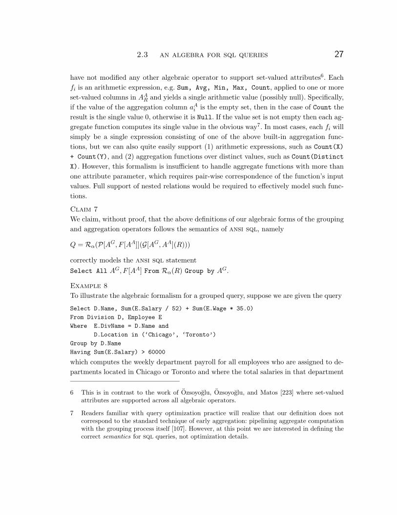
2.3 an algebra for sql queries 27
have not modified any other algebraic operator to support set-valued attributes6. Eachfi is an arithmetic expression, e.g. Sum, Avg, Min, Max, Count, applied to one or moreset-valued columns in AA
R and yields a single arithmetic value (possibly null). Specifically,if the value of the aggregation column aAi is the empty set, then in the case of Count theresult is the single value 0, otherwise it is Null. If the value set is not empty then each ag-gregate function computes its single value in the obvious way7. In most cases, each fi willsimply be a single expression consisting of one of the above built-in aggregation func-tions, but we can also quite easily support (1) arithmetic expressions, such as Count(X)+ Count(Y), and (2) aggregation functions over distinct values, such as Count(DistinctX). However, this formalism is insufficient to handle aggregate functions with more thanone attribute parameter, which requires pair-wise correspondence of the function’s inputvalues. Full support of nested relations would be required to effectively model such func-tions.
Claim 7
We claim, without proof, that the above definitions of our algebraic forms of the groupingand aggregation operators follows the semantics of ansi sql, namely
Q = Rα(P[AG, F [AA]](G[AG, AA](R)))
correctly models the ansi sql statementSelect All AG, F [AA] From Rα(R) Group by AG.
Example 8
To illustrate the algebraic formalism for a grouped query, suppose we are given the query
Select D.Name, Sum(E.Salary / 52) + Sum(E.Wage * 35.0)
From Division D, Employee E
Where E.DivName = D.Name and
D.Location in (‘Chicago’, ‘Toronto’)
Group by D.Name
Having Sum(E.Salary) > 60000
which computes the weekly department payroll for all employees who are assigned to de-partments located in Chicago or Toronto and where the total salaries in that department
6 This is in contrast to the work of Ozsoyoglu, Ozsoyoglu, and Matos [223] where set-valuedattributes are supported across all algebraic operators.
7 Readers familiar with query optimization practice will realize that our definition does notcorrespond to the standard technique of early aggregation: pipelining aggregate computationwith the grouping process itself [107]. However, at this point we are interested in defining thecorrect semantics for sql queries, not optimization details.

28 preliminaries
must be greater than $60,000. In terms of our formalisms for sql semantics we expressthis query as
πAll[aG1 , f1](σ[Ch](P[AG, F [AA] ](G[AG, AA](σ[C](E × D))))) (2.14)
where
• D and E are extended tables corresponding to the employee and division tablesrespectively.
• AG are the grouping attributes; specifically aG1 is the attribute D.Name.
• P is of degree 3 and consists of the grouping attribute D.Name and the two aggre-gation function expressions f1 and f2 in F . Expression f1 computes the sum of thesums defined over the aggregation columns E.Salary and E.Wage. Expression f2
computes the sum of E.Salary required for the evaluation of the Having clause.
• Ch represents the Having predicate which compares the result of applying the ag-gregation function f2 (the grouped sum of E.Salary) to the aggregation attributeE.Salary to the constant value 60,000.
• G represents the partitioning of the join of division and employee over the group-ing attribute D.Name and forming the three set-valued columns aA1 , a
A2 , and a
A3 from
the base attributes E.Salary (twice) and E.Wage, respectively;
• C = CD,E ∧CD represents the two predicates in the query’s Where clause, the firstbeing the join predicate and the second representing the restriction on division.
2.3.2 Query expressions
Definition 19 (Union-compatible tables)
Two tables T1 = 〈{a1, a2, . . . , an}, ι1, κ1, ρ1, E1〉 and T2 = 〈{b1, b2, . . . , bn}, ι2, κ2, ρ2, E2〉are said to be union-compatible if and only if the domains of their corresponding realattributes are identical, that is Domain(ai) = Domain(bi) for 1 ≤ i ≤ n. We representthis correspondence by the function bi = corr(ai).
Definition 20 (Union)
The union of two union-compatible extended tables S and T , written S ∪All T producesan extended table R′ as its result with schema attributes as follows:
• α(R′) = α(S);
• ι(R′) = a new tuple identifier attribute;

2.3 an algebra for sql queries 29
• κ(R′) = κ(S) ∪ κ(T );
• ρ(R′) = ρ(S) ∪ ρ(T ) ∪ ι(S) ∪ ι(T ) ∪ α(T ).
Note that we have arbitrarily chosen to model the real set of attributes in R′ using thosereal attributes from S.
The instance I(R′) is constructed as follows. Similarly to full outer join (see Defini-tion 16 above) we construct two tuples sNull and tNull as ‘placeholders’ for missing at-tribute values. Then I(R′) is:
I(R′) = R{r′ | (∃ s ∈ I(S) : r′[sch(S)] ω= s[α(S)] ∧ r′[sch(T )] ω= tNull[sch(T )]) (2.15)
∨ (∃ t ∈ I(T ) : (∀ a ∈ α(S) : r′[a] ω= t[corr(a)]) ∧r′[sch(T )] ω= t[sch(T )] ∧ r′[sch(S) \ α(S)] ω= sNull[sch(S) \ α(S)]) }.
Claim 8
The expression
Q = Rα(S ∪All T )
correctly models the ansi sql statement
Select * From Rα(S)Union All
Select * From Rα(T ).
Definition 21 (Distinct Union)
The distinct union of two union-compatible extended tables S and T , written S ∪Dist T
produces an extended table R′ equivalent to the expression πDist [α(S ∪All T )](S ∪All T ).
Claim 9
The expression
Q = Rα(S ∪Dist T )
correctly models the ansi sql statement
Select * From Rα(S)Union
Select * From Rα(T ).

30 preliminaries
Definition 22 (Difference)
The difference of two union-compatible extended tables S and T , written S −All T pro-duces an extended table R′ with sch(R′) = sch(S). The semantics of difference are as fol-lows. Let s0 denote a tuple in I(S) and t0 a tuple in I(T ) such that s0[α(S)]
ω= t0[α(T )].Let j ≥ 1 be the number of occurrences of tuples in I(S) such that s[α(S)] ω= s0[α(S)],and let k similarly be the number of occurrences (possibly 0) of t0 in I(T ). Then the num-ber of instances of s0 that occur in the result I(R′) is the maximum of j − k and zero; ifj > k ≥ 1 then we select j − k tuples of I(S) nondeterministically.
Claim 10
The expression
Q = Rα(S −All T )
correctly models the ansi sql statement
Select * From Rα(S)Except All
Select * From Rα(T ).
Definition 23 (Distinct difference)
The distinct difference, or difference with duplicate elimination, of two union-compatibleextended tables S and T , written S−Dist T , produces an extended table R′ equivalent tothe expression πDist [α(S −All T )](S −All T ).
Claim 11
The expression
Q = Rα(S −Dist T )
correctly models the ansi sql statement
Select * From Rα(S)Except
Select * From Rα(T ).
Definition 24 (Intersection)
The intersection of two union-compatible extended tables S and T , written S ∪All T pro-duces an extended table R′ with schema:
• α(R′) = α(S);

2.3 an algebra for sql queries 31
• ι(R′) = ι(S);
• κ(R′) = κ(S) ∪ κ(T );
• ρ(R′) = ρ(S) ∪ ρ(T ) ∪ ι(T ).
The semantics of intersection are as follows. Let s0 denote a tuple in I(S) and t0 a tuplein I(T ) such that s0[a]
ω= t0[corr(a)] for all a ∈ α(S). Let j ≥ 1 be the number of occur-rences of tuples in I(S) such that s[α(S)] ω= s0[α(S)], and let k ≥ 1 similarly be the num-ber of occurrences of t0[α(T )] in I(T ). Then the number of occurrences of s0 in the re-sult I(R′) of the intersection of these two subsets of tuples is the minimum of j and k. Letm be the absolute value of j − k. We construct the m tuples r′ ∈ I(R′) as follows. Non-deterministically select m tuples s1, s2, . . . , sm from the j occurrences matching s0[α(S)]in I(S). Similarly, nondeterministically select m tuples t1, t2, . . . , tm from the k occur-rences matching t0[α(T )] ∈ I(T ). Now construct the m tuples r′1, r′2, . . . , r′m such that
r′i[sch(S)]ω= si[sch(S)] ∧ r′i[ρ(T ) ∪ ι(T ) ∪ κ(T )] ω= ti[ρ(T ) ∪ ι(T ) ∪ κ(T )]
for 1 ≤ i ≤ m. Constructing I(R′) in this manner for each set of matching tuples in S
and T gives the entire result.
Claim 12
The expression
Q = Rα(S ∩All T )
correctly models the ansi sql statement
Select * From Rα(S)Intersect All
Select * From Rα(T ).
Definition 25 (Distinct intersection)
The distinct intersection of two union-compatible extended tables S and T , writtenS ∩Dist T , produces an extended table R′ consisting of the intersection of S and T withduplicates removed, and is equivalent to the expression πDist [α(S ∩All T )](S ∩All T ).
Claim 13
The expression
Q = Rα(S ∩Dist T )

32 preliminaries
correctly models the ansi sql statement
Select * From Rα(S)Intersect
Select * From Rα(T ).
2.4 Functional dependencies as constraints
Intensional data such as integrity constraints offer an important form of metadata thatcan be exploited during query optimization [50, 105, 114, 161, 205, 258, 260, 282, 283, 293].Ullman [277], Fagin [87], Casanova et al. [45], Sadri and Ullman [243], and Missaoui andGodin [204] offer surveys of various classes of integrity constraints. These constraints formtwo major classes: inclusion dependencies and functional dependencies.
Functional dependencies are a broad class of data dependencies that have been widelystudied in the relational database literature (cf. references [13, 14, 23, 45, 77, 83, 85, 86, 88,128, 185, 206, 281]). A ‘classical’ formal definition of a functional dependency is as follows[45]. Consider the relation scheme R(A) with attributes A = {a1, . . . , an}. Let A1 ⊆ A
and A2 ⊆ A denote two subsets of A (not necessarily disjoint). Then we call the depen-dency
R : A1 −→ A2 (2.16)
a functional dependency of A2 on A1 and say that R satisfies the functional dependencyif whenever tuples r1, r2 ∈ R and r1[A1] = r2[A1], then r1[A2] = r2[A2].
Exploiting inclusion and functional dependencies in query optimization relies upontheir discovery. ansi sql defines several mechanisms for declaring constraints, which wenow describe in some detail. The main difference between ‘classical’ constraint defini-tions, such as that for functional dependencies, and those permitted in ansi sql is thatthe classical definitions utilize two-valued logic, whereas the semantics of sql constraintshave to take into account the existence of null values.
2.4.1 Constraints in ANSI SQL
The schema definition mechanisms in ansi sql permit the specification of a wide vari-ety of constraints on database instances. For example, a Not Null constraint on a col-umn definition imposes the obvious restriction that no tuple can contain a null value forthat attribute. Integrity constraints in ansi sql consist of two major classes, column con-straint definitions and table constraint definitions.

2.4 functional dependencies as constraints 33
A column constraint may reference either a specific domain or a Check clause, whichdefines a search condition that cannot be false (thus the predicate is true-interpreted).For example, the check constraint definition for column EmpID in employee could beCheck (EmpID Between 1 and 100). A tuple in employee violates this constraint if itsEmpID value is not Null and lies outside this range. Check constraints on domains areidentical to Check constraints on columns and typically specify ranges of possible values.
There are several different forms of table constraints. A Check clause that is speci-fied as part of a table constraint in ansi sql can subsume any column or domain con-straint; furthermore the condition can specify conditions that must hold between multi-ple attributes. Other forms of table constraints include referential integrity constraints(primary key and foreign key definitions) and Unique constraint definitions that definecandidate keys. In each form of table constraint there is an implicit range variable refer-encing the table over which the constraint is defined. More general constraints, termedAssertions, relax this requirement and permit the specification of any sql expression(hence range variables are explicit).
In this thesis we consider Not Null column constraints and two forms of table con-straints. Check constraints on base tables in sql2 identify conditions for columns in a ta-ble that must always evaluate to true or unknown. For example, our division table isdefined as:
Create Table Division (
Name ..., Location ..., ManagerID ...
Primary Key (Name),
Check (Location in (‘Chicago’, ‘New York’, ‘Toronto’)))
which specifies a Check condition on Location. Since this condition cannot be false, thenthe query
Select * From Division
Where Location in
(‘Chicago’, ‘New York’, ‘Toronto’) or
Location is null
must return all tuples of division. What this means is that we can add any table con-straint to a query (suitably adjusted to account for null values) without changing the queryresult.
The second type of table constraint we consider is a unique specification that iden-tifies a primary or candidate key. Our interest in keys is because they explicitly definea functional dependency between the key columns and the other attributes in the ta-ble. There are three sources of unique specifications:
• primary key specifications,
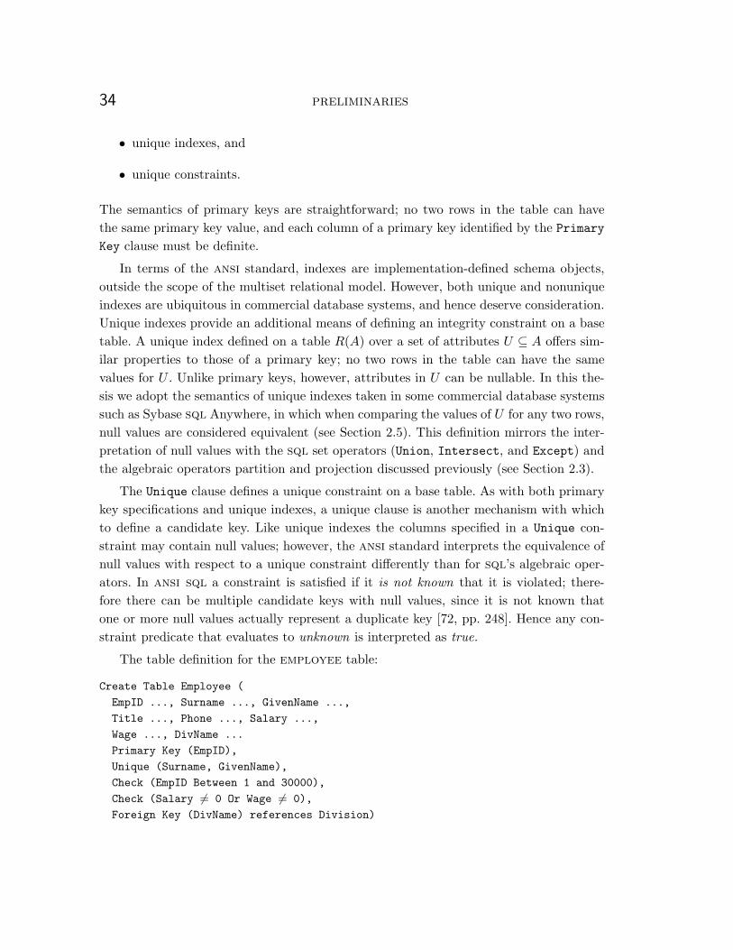
34 preliminaries
• unique indexes, and
• unique constraints.
The semantics of primary keys are straightforward; no two rows in the table can havethe same primary key value, and each column of a primary key identified by the PrimaryKey clause must be definite.
In terms of the ansi standard, indexes are implementation-defined schema objects,outside the scope of the multiset relational model. However, both unique and nonuniqueindexes are ubiquitous in commercial database systems, and hence deserve consideration.Unique indexes provide an additional means of defining an integrity constraint on a basetable. A unique index defined on a table R(A) over a set of attributes U ⊆ A offers sim-ilar properties to those of a primary key; no two rows in the table can have the samevalues for U . Unlike primary keys, however, attributes in U can be nullable. In this the-sis we adopt the semantics of unique indexes taken in some commercial database systemssuch as Sybase sql Anywhere, in which when comparing the values of U for any two rows,null values are considered equivalent (see Section 2.5). This definition mirrors the inter-pretation of null values with the sql set operators (Union, Intersect, and Except) andthe algebraic operators partition and projection discussed previously (see Section 2.3).
The Unique clause defines a unique constraint on a base table. As with both primarykey specifications and unique indexes, a unique clause is another mechanism with whichto define a candidate key. Like unique indexes the columns specified in a Unique con-straint may contain null values; however, the ansi standard interprets the equivalence ofnull values with respect to a unique constraint differently than for sql’s algebraic oper-ators. In ansi sql a constraint is satisfied if it is not known that it is violated; there-fore there can be multiple candidate keys with null values, since it is not known thatone or more null values actually represent a duplicate key [72, pp. 248]. Hence any con-straint predicate that evaluates to unknown is interpreted as true.
The table definition for the employee table:
Create Table Employee (
EmpID ..., Surname ..., GivenName ...,
Title ..., Phone ..., Salary ...,
Wage ..., DivName ...
Primary Key (EmpID),
Unique (Surname, GivenName),
Check (EmpID Between 1 and 30000),
Check (Salary �= 0 Or Wage �= 0),
Foreign Key (DivName) references Division)

2.5 sql and functional dependencies 35
defines a Check constraint on salary and hourly wage, along with the composite candi-date key (Surname, GivenName), in addition to the specified primary and foreign keyconstraints.
2.5 SQL and functional dependencies
Because the ansi sql standard permits a Unique constraint over nullable attributes, nullvalues may exist on both the left- and right-hand sides of a functional dependency in bothbase and derived tables. To show that such a functional dependency holds for any twotuples t0 and t1, we must be able to compare both the determinant and dependent valuesof the two tuples. Such comparisons involving null values must follow ansi sql semanticsfor three-valued logic. Using the null interpretation operator (Definition 11) and the nullcomparison operator ω= (Definition 6) we formally define functional dependencies in thepresence of nulls as follows:
Definition 26 (Functional dependency)
Consider an extended table R and sets of attributes A1 ⊆ sch(R) and A2 ⊆ sch(R) whereA1 and A2 are not necessarily distinct. Let I(R) denote a specific instance of R. Then A1
functionally determines A2 in I(R) (written A1I(R)−→ A2) if the following condition holds:
∀ t0, t′0 ∈ I(R) : t0[A1]ω= t′0[A1] =⇒ t0[A2]
ω= t′0[A2].
In other words, if the functional dependency holds and two tuples agree on the set ofattributes A1, then the two tuples must agree on the value of the attributes in A2. Notethe treatment of null values implicit in this definition: corresponding attributes in A1 andA2 must either agree in value, or both be Null.
Table definitions serve to define constraints (nullability, primary keys, table and col-umn constraints) that must hold for every instance of a table. Consequently we assumethat any constraint in an extended table definition automatically applies to every in-stance of that table. Hence we write A1 −→ A2 when I(R) is clear from the context.
From Definition 26 we can now formally define a key dependency.
Definition 27 (Key Dependency)
Consider an extended table R. Let I(R) denote an instance of R. Let K denote somesubset of sch(R). Then K is a key of R if and only if the following functional dependencyholds:
K −→ ι(R). (2.17)

36 preliminaries
This formalism merely states our intuitive notion of a key: no two distinct tuples mayhave the same key.
2.5.1 Lax functional dependencies
It is precisely our interpretation of null values as ‘special’ values in each domain—and cor-respondingly, our use of Negri’s null interpretation operator to test their satisfaction us-ing three-valued logic—that differentiates our approach to the handling of null valueswith respect to functional dependencies from other schemes that introduce the notion of‘weak dependency’ (cf. Section 2.5.3 below). Following convention, our definition of func-tional dependency, which we term strict, only permits strong satisfaction in the sense thatthe constraint defined by Definition 26 must evaluate to true. However, due to the ex-istence of (1) nullable attributes in Unique constraints, (2) true-interpreted predicatesformed from Check constraints or through the conversion of a nested query into a canon-ical form, and (3) the semantics of outer joins, we must also define a weaker form of func-tional dependency, which we term a lax functional dependency8.
Definition 28 (Lax functional dependency)
Consider an extended table R and sets of attributes A1 ⊆ sch(R) and A2 ⊆ sch(R) whereA1 and A2 are not necessarily distinct. Let I(R) denote a specific instance of R. Then A1
laxly determines A2 in I(R) (written A1I(R)&−→ A2) if the following condition holds:
∀ t0, t′0 ∈ I(R) : � t0[A1] = t′0[A1] � =⇒ � t0[A2] = t′0[A2] �.
Unlike strict dependencies, both the antecedent and consequent expressions must be equalonly for non-null determinant and dependent values, which corresponds to the classicaldefinition of functional dependency [13]. Again we write A1 &−→ A2 when I(R) is clearfrom the context. Henceforth when we use the term ‘dependency’ without qualificationwe mean either a strict or lax functional dependency.
By themselves, lax functional dependencies are not that interesting since they can-not guarantee anything about the relationship between their left- and right-hand sides ifeither side includes nullable attributes (the conditions in Definitions 26 and 28 are equiv-alent if every attribute in the determinant and dependent sets cannot be Null). However,they are worth capturing because there are circumstances in which we can convert lax de-pendencies into strict ones.
8 We use the term ‘lax’ to avoid any confusion with other definitions of ‘weak’ functional de-pendencies; see Section 2.5.3.

2.5 sql and functional dependencies 37
Example 9 (Lax dependency conversion)
Consider the following query over the supply and vendor tables:
Select Distinct V.Name, V.ContactName, V.Address, S.PartID, S.Rating
From Vendor V, Supply S
Where V.Name like :Pattern and V.VendorID = S.VendorID
where :Pattern is a host variable containing the pattern for desired vendor names. Fromthe Unique constraint declared in the definition of the vendor table, the attribute Nameconstitutes a candidate key, and thus laxly determines each of the other attributes in ven-dor. However, the false-interpreted, null-intolerant9 like predicate will eliminate fromthe result any rows from vendor which have unknown names, ensuring the uniquenessof V.Name attributes. Hence V.Name and S.PartID together form a derived key depen-dency in the result, and we can infer that duplicate elimination is not necessary.
2.5.2 Axiom system for strict and lax dependencies
Although Definition 26 extends the equivalence relationship between two attributes to in-clude null values, the inference rules, known as Armstrong’s axioms [13], used to inferadditional functional dependencies still hold: all that we have really done is to define anequivalence relationship between null values in each domain. However, we need to aug-ment these inference rules to support lax functional dependencies. In this section, we de-scribe a set of sound inference rules for a combined set of strict and lax dependencies cor-responding to Definitions 26 and 28 respectively.
Lemma 1
The following inference rules, defined over an instance I(R) of an extended table R withsubsets of attributes X,Y, Z,W ⊆ sch(R), are sound:
9 A null-intolerant predicate is one which cannot evaluate to true if any of the predicate’soperands are Null. In ansi sql, virtually all false-interpreted comparison predicates, Likepredicates, and similar search conditions are null-intolerant. A simple example of a null-tolerant predicate is p is null.

38 preliminaries
X Y Z
3 Null 53 Null 3
Figure 2.1: An instance of table Rα(R).
Reflexivity fd1 If Y ⊆ X then X −→ Y .Augmentation fd2a If X −→ Y and Z ⊆W then XW −→ Y Z.
fd2b If X &−→ Y and Z ⊆W then XW &−→ Y Z.Union fd3a If X −→ Y and X −→ Z then X −→ Y Z.
fd3b If X &−→ Y and X &−→ Z then X &−→ Y Z.Strict decomposition fd4a If X −→ Y Z then X −→ Y and X −→ Z.Weakening fd5 If X −→ Y then X &−→ Y .Strengthening fd6 If X &−→ Y and I(R) is XY -definite then X −→ Y .Strict transitivity fd7a If X −→ Y and Y −→ Z then X −→ Z.
Proof. Omitted. ✷
Note that, in general, transitivity does not hold for lax dependencies in the same waythat transitive relationships break down for other definitions of weak dependencies [17][16, pp. 243]. Consider the table instance shown in Figure 2.1. It is easy to see that thestrict functional dependency X −→ Y and the lax functional dependency Y &−→ Z bothhold. However, note that neither X −→ Z nor X &−→ Z hold; the problem, of course,is that the definition of a lax functional dependency means that Null attributes cannotlead to a dependency violation. However, transitivity of a lax dependency over definite at-tributes is sound since eliminating Null determinants and dependents yields a functionaldependency with the same semantics as one that is strict.
Lemma 2 (Transitivity of lax dependencies)
The inference rule:
Lax transitivity fd7b If X &−→ Y and Y &−→ Z and I(R) is Y -definite then X &−→ Z.
defined over an instance I(R) of an extended table R with subsets of attributes X,Y, Z ⊆sch(R), is sound.
Proof. Consider an instance I(R) of an extended table R where XY Z ⊆ sch(R) andI(R) is Y -definite. By contradiction, assume that I(R) |= X &−→ Y and Y &−→ Z but
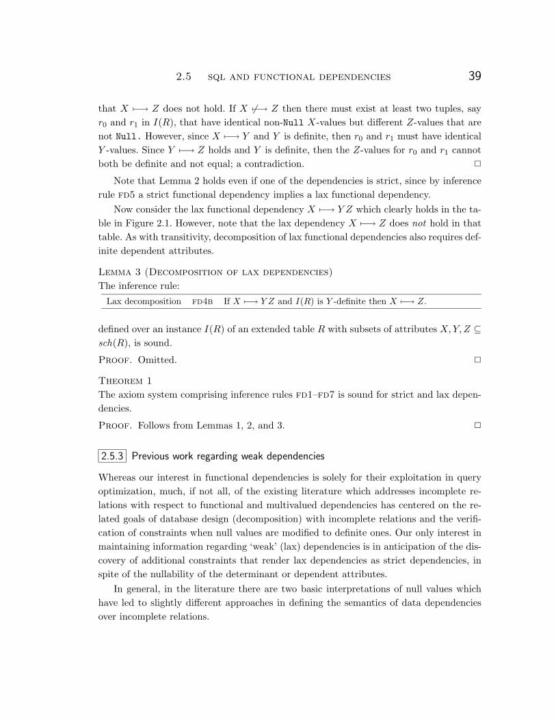
2.5 sql and functional dependencies 39
that X &−→ Z does not hold. If X �&−→ Z then there must exist at least two tuples, sayr0 and r1 in I(R), that have identical non-Null X-values but different Z-values that arenot Null. However, since X &−→ Y and Y is definite, then r0 and r1 must have identicalY -values. Since Y &−→ Z holds and Y is definite, then the Z-values for r0 and r1 cannotboth be definite and not equal; a contradiction. ✷
Note that Lemma 2 holds even if one of the dependencies is strict, since by inferencerule fd5 a strict functional dependency implies a lax functional dependency.
Now consider the lax functional dependency X &−→ Y Z which clearly holds in the ta-ble in Figure 2.1. However, note that the lax dependency X &−→ Z does not hold in thattable. As with transitivity, decomposition of lax functional dependencies also requires def-inite dependent attributes.
Lemma 3 (Decomposition of lax dependencies)
The inference rule:
Lax decomposition fd4b If X &−→ Y Z and I(R) is Y -definite then X &−→ Z.
defined over an instance I(R) of an extended table R with subsets of attributes X,Y, Z ⊆sch(R), is sound.
Proof. Omitted. ✷
Theorem 1
The axiom system comprising inference rules fd1–fd7 is sound for strict and lax depen-dencies.
Proof. Follows from Lemmas 1, 2, and 3. ✷
2.5.3 Previous work regarding weak dependencies
Whereas our interest in functional dependencies is solely for their exploitation in queryoptimization, much, if not all, of the existing literature which addresses incomplete re-lations with respect to functional and multivalued dependencies has centered on the re-lated goals of database design (decomposition) with incomplete relations and the verifi-cation of constraints when null values are modified to definite ones. Our only interest inmaintaining information regarding ‘weak’ (lax) dependencies is in anticipation of the dis-covery of additional constraints that render lax dependencies as strict dependencies, inspite of the nullability of the determinant or dependent attributes.
In general, in the literature there are two basic interpretations of null values whichhave led to slightly different approaches in defining the semantics of data dependenciesover incomplete relations.

40 preliminaries
2.5.3.1 Null values as unknown
The first approach to the problem of defining the semantics of data dependencies in in-complete relations involves the substitution, or possible substitution, of a null value witha definite one. This is usually referred to as the ‘value exists but is unknown’ interpreta-tion of Null, in that the null value represents some unknown quantity in the real world:i.e. if attribute X in tuple t is Null there exists a value for t[X], but this value is presentlyunknown. Implicit in this approach is an assumption that all null values are ‘indepen-dent’, in that each null value in the database can be substituted with some definite valuefrom that attribute’s domain (subject to other constraints in the database). This inter-pretation of Null has been previously studied by Codd [66], Biskup [35], Grant [115], andMaier [193]. In general, the satisfaction of a functional dependency in this approach de-pends on whether or not some definite value can be substituted for a null value such thatthe dependency holds [113].
Vassiliou [286, 287] pioneered the study of null values with respect to dependency the-ory. He defined a weak dependency as a constraint having the capacity to substitute nullvalues with some set of arbitrary non-null ones that would fail to render a given depen-dency patently false (the domains of all attributes are assumed known and finite). Be-low we reiterate Vassiliou’s Proposition 1 [287, pp. 263] that defines his satisfaction cri-teria for functional dependencies.
Proposition 1 (Vassiliou’s axioms for satisfaction of fds)
Let R(U) be a relation scheme with X∪Y = U such that X∩Y = ∅, and let f : X −→ Y
be a functional dependency in R. Let t denote a tuple in I(R). Assume that I(R) − t
is definite, or alternatively consider all completions of I(R)− t iteratively. Then f holdswith respect to t iff one of the following conditions holds:
1. t is XY -definite and there exists no tuple t′ ∈ I(R) such that t′[X] = t[X] andt′[Y ] �= t[Y ].
2. t is X-definite and X uniquely occurs in I(R).
3. t is Y -definite and either no completion of t[X] is in I(R), or if a completion of t[X]is in I(R), say t′[X], then t[Y ] = t′[Y ].
f fails to hold with respect to t ∈ I(R) iff one of the following conditions holds:
1. t is XY -definite and there exists a tuple t′ ∈ I(R) such that t′[X] = t[X] andt′[Y ] �= t[Y ], or
2. t is Y -definite and both

2.5 sql and functional dependencies 41
(a) all completions of t[X] appear in I(R), and
(b) t[Y ] is unique among all those completions.
Aside. Since Vassiliou deals with relations, not multisets, this last rule means thatany null substitution within t[X] either cannot be permitted due to a domain con-straint on X, or will result in a duplicate row in I(R). This rule can also lead toan inconsistency where f may not be false for each pair of tuples r0, r1 ∈ I(R) in-dependently, but f may be false in the whole relation. This problem is often re-ferred to as the additivity problem for functional dependencies in incomplete rela-tions [177, 179].
Otherwise, it is unknown if f holds with respect to t in I(R).
With these conditions, a functional dependency f strongly holds if f holds for each tuplet in I(R), and weakly holds if f does not fail to hold for any t. Vassiliou went on toshow that Armstrong’s axioms [13] form a sound and complete set of inference axiomsfor functional dependencies that strongly hold.
The above work considers a single set of dependencies over a database possibly con-taining null values, where each dependency can either strongly or weakly hold depend-ing on the particular instance. In a recent paper, Levene and Loizou [179] develop defini-tions of strong and weak functional dependencies and an axiomatization for a combinedset of the two distinct types. As with Vassiliou, dependency satisfaction relies on the sub-stitution of null values. They use the following definition, which we state here informally,to describe this substitution:
Definition 29 (Possible worlds of a relation R)
The set of all possible worlds relative to an instance I(R) of a relation R, which we denotePOSS(I(R)), is
POSS(I(R)) = {I(S) | I(S) is a relation over R and there exists a total andonto mapping f : I(R)→ I(S) such that ∀ t ∈ I(R),f(t) is complete (that is, each attribute in f(t) isdefinite).
(2.18)
With this definition of substitution, the satisfaction of a functional dependency is de-fined as follows:
• Strong satisfaction: the strong dependency f : X −→ Y holds in a relation I(R)over R if and only if there exists at least one possible world (POSS(I(R)) �= ∅)and for all such possible worlds s ∈ POSS(I(R)), ∀ t0, t1 ∈ s, if t0[X] = t1[X] thent0[Y ] = t1[Y ].

42 preliminaries
Loosely speaking, this definition is less restrictive than our definition of strict func-tional dependency (Definition 26) since our definition equates two null values, whichcorresponds to the null equality constraint defined by Vassiliou [287, Definition 1].
• Weak satisfaction: the weak dependency f : X &−→ Y holds if and only if thereexists at least one possible world s ∈ POSS(I(R)) such that ∀ t0, t1 ∈ s, if t0[X] =t1[X] then t0[Y ] = t1[Y ].
This definition is incomparable to our definition of lax dependency, simply becausewe do not rely on substitution but instead omit from consideration any tuple t ∈I(R) that is not XY -definite.
With these definitions, Levene and Loizou go on to describe a sound and complete ax-iom system for the combined set of strong and weak functional dependencies. Their defi-nitions permit the inference of strong dependencies from a mixed set of strong and weakdependencies (their inference rule FD9 ).
2.5.3.2 Null values as no information
The second approach, more simplistic than the first, is to interpret Null as represent-ing no information [300, 302]. In essence this means avoiding any attempt at value sub-stitution as the null value can represent ‘unknown’, ‘undefined’, ‘nonexistent’, or ‘inap-plicable’ values [183].
Independently from Vassiliou10, Lien [183][184, Section 4.1] considered multivalued de-pendencies with null values and functional dependencies with null values, which he ab-breviated nmvds and nfds respectively. An nfd f : X −→ Y is satisfied if
∀ r0, r1 ∈ I(R) : � r0[X] = r1[X] � =⇒ r0[Y ]ω= r1[Y ]. (2.19)
With this definition Lien showed that his inference rulesReflexivity f1 If Y ⊆ X then X −→ Y .Augmentation f2 If X −→ Y and Z ⊆W then XW −→ Y Z.Union f3 If X −→ Y and X −→ Z then X −→ Y Z.Decomposition f4 If X −→ Y Z then X −→ Y and X −→ Z.
were all sound with respect to nfds, but notably transitivity (or pseudotransitivity) wasnot (see Figure 2.1).
10 There are no corresponding references from Lien’s work [183, 184] to either of Vassiliou’s earlypapers [286, 287] on null values in relational databases, or vice-versa.

2.6 overview of query processing 43
Atzeni and Morfuni [17] also defined nfds on the basis of definite determinants (2.19)and the ‘no information’ interpretation of null values. In this short paper they introduceda modified version of Armstrong’s transitivity axiom, which they termed null-transitivity,that relied on definite dependent attributes. Atzeni and Morfuni go on to show that theirnull-transitivity axiom, which is quite similar to the lax-transitivity inference rules inLemma 2 above, and Lien’s inference rules f1 through f4 form a sound and complete setof inference rules for nfds; a more detailed version of the proof can be found in refer-ence [18].
Related work on functional dependencies over incomplete databases have been ad-dressed by Maier [193, pp. 377–86], Imielinski and Lipski [134], Abiteboul et al. [4, pp. 497–8], Zaniolo [300, 302], Libkin [182], Levene [176], Levene and Loizou [177, 178, 180], andAtzeni and De Antonellis [16, pp. 239–48]).
2.6 Overview of query processing
Several excellent references regarding the complete framework of query optimization existin the literature [51, 71, 107, 143, 193, 203, 278, 299]. We define centralized, as opposed todistributed, query optimization as the following sequence of steps:
1. Find an internal representation into which user queries11 can be cast. This repre-sentation must typically be richer than either classical relational calculus or alge-bra, due to language extensions such as scalar and aggregate functions, outer joins,duplicate rows, and null values. One example of an internal representation is theQuery Graph Model used in starburst [124].
2. Apply rewriting transformations to the query to standardize it by rewriting it intoa canonical form, simplify it by eliminating redundancy, and improve (ameliorate)it if possible. This process also combines the query with the view definitions of theschema [71, 186, 267]. The point is that the performance of a query should not de-pend on how the query was cast originally by the user [71, pp. 459]. Many query lan-guages, including sql, allow queries to be expressed in several equivalent, thoughsyntactically different, forms.
3. Generate access plans for each transformed query by mapping each of them into se-quences of lower-level operations, and augment these plans with information aboutthe physical characteristics of the database.
11 In this context, the term ‘query’ not only refers to retrieval operations, but also (and perhapsmore importantly) to database updates.

44 preliminaries
4. Choose the best access plan alternative, depending on the cost of each plan and theperformance goals of the optimizer (resource or response time minimization).
5. Generate a detailed query execution plan that captures all necessary informationto execute the plan.
6. At run time, execute the detailed plan.
2.6.1 Internal representation
The first stage of query processing is the conversion of the syntactic statement into an in-ternal representation that constitutes the statement’s canonical form—where extraneoussyntax has been eliminated and view definitions have been expanded—that is suitable foranalysis by an optimizer. A typical representation for an sql request, and the one usedherein, is an algebraic expression tree [193, pp. 296–314] [278]. One can think of this ex-pression tree as an annotated parse tree that models the semantics of the query usingunary (projection, restriction) and binary (inner join, outer join) operators with struc-tures representing base tables at the leaves.
Example 10
Consider the query
Select P.PartID, P.Description, S.SupplyCode, V.VendorID, V.Name
From Parts P Left Outer Join
(Supply S Join Vendor V On ( S.VendorID = V.VendorID )
On ( P.PartID = S.PartID and V.Address like ‘%Canada%’ )
Where Exists ( Select *
From Quote Q
Where Q.PartID = P.PartID and
Q.Date ≥ ‘1993-10-01’ )
which retrieves those parts that have received quotes at any time since 1 October 1993,along with the vendors of any of those parts that have Canadian addresses. Figure 2.3 il-lustrates a straightforward mapping of this query into a relational algebra tree. Note thatthe operators used for the nested subquery are distinct from the operators that repre-sent the main query block.
The algebraic expression tree is a restricted form of an acyclic12 directed graph. Ver-tices in the tree represent unary or binary algebraic operators and have one outgoing edge
12 We remind the reader that in this thesis we restrict the class of queries considered to nonre-cursive queries.

2.6 overview of query processing 45
Plan Storage
Query RewriteSyntactic and
semantictransformationsView integration
Plan GenerationJoin orderingJoin methods
Index selectionPredicate placementGrouping techniques
Parsing and Semantic Checking
Plan Selection
DetailedPlan Creation
Query
Semantic transformation rulesHeuristicsIntegrity constraintsExtensional informationPhysical storage organizationCatalog information
Physical algebra transformationsHeuristicsAccess path informationPhysical storage organizationIntegrity constraintsCatalog information
Performance goalsStatisticsEstimatesCost model
Catalog information
Inte
rnal
Qu
ery
Rep
rese
nta
tio
n
Plan Execution
Query Result
Catalog information
Figure 2.2: Phases of query processing. For simplicity, each phase is shown as a inde-pendent step; however, some processing overlap is inevitable, especially in limiting thenumber of alternative execution strategies generated in the query rewrite and plan gen-eration. Inputs to each phase are shown on the right.

46 preliminaries
Π
σ
σ
Project P.PartID, P.Description, S.SupplyCode, V.VendorID, V.Name
Restricton Q.PartID,Q.Date
Restrict onsubquery result
Left Outer Join onP.PartID = S.PartID andV.Address like '%Canada%'
Join on S.VendorID = V.VendorID
Part
Supply Vendor
Quote
Subquery Block
P.PartID
Figure 2.3: Example relational algebra tree for the query in Example 10.
and either one (for the unary operators projection and restriction) or two (for the binaryoperators join, outer join, set union, etc.) incoming edges. The directed edges in the graphrepresent data flowing up the tree from the leaves to the root; the outgoing edge at thetree’s root represents tuples returned as part of the query’s result. Note that a unary op-erator can appear anywhere in the tree. For example, an equivalent form of the expres-sion tree in Figure 2.3 is one where the Exists predicate is placed immediately above thenode representing the Part base table. Placing the subquery at that point corresponds toa naive predicate pushdown approach [263] and is possible because the range of the sub-query only consists of the single attribute PartID from the part table.
Each node in the tree is typically annotated in that the output edge of each node islabelled with the attributes that are returned as part of that tuple stream, along withtheir data types. View information is often retained, even if the views are completelymerged into the query (see Section 2.6.2.2), because subsequent operations—for exam-ple, an Update ... Where Current of Cursor statement—can (and must) refer to theoriginal objects specified in the query.

2.6 overview of query processing 47
Subqueries in a Where or Having clause are modelled by constructing a separate, in-dependent expression tree, but are connected through an alternate form of edge to a re-striction node in the subquery’s parent query block13. In Figure 2.3, the nested queryblock representing the Exists predicate in the example does not contain a projectionsince a projection is irrelevant in the context of an Exists predicate.
In several commercial systems, including db2, sybase sql Anywhere, and sybaseiq, algebraic expression trees form the basis for preliminary query optimization analy-sis and rewrite optimization [90, 187, 230] though their implementations may differ some-what from the expression trees described herein. For example, starburst [121, 187] mod-els queries using Logical Plan Operators (lolepops) that represent a richer set of alge-braic operators than that described here. Like starburst, Graefe’s Volcano executionmodel [108, 110, 112] also represents query plans using executable algebraic operators, butpermits the operators to be organized into any tree structure so long as it adheres to Vol-cano’s demand-driven data flow paradigm. Volcano’s extensible architecture permits oneto implement any algebraic operation that supports Volcano’s three standardized itera-tion operations, namely Open, Next, and Close. Hence specialized algebraic operationssuch as Dayal’s [74] Generalized Join or existence-semijoin can constitute portions of theexpression tree. We do not consider these types of executable algebraic operations in thisthesis, though the techniques presented here could be readily adapted to encompass thesespecialized operators.
In the following sections we provide a brief overview of the optimization phases ofquery rewrite, plan generation, and plan selection, beginning with query rewrite.
2.6.2 Query rewrite optimization
Query rewriting, often termed semantic query optimization, is the process of generat-ing semantically equivalent queries from the original to give the optimizer a wider rangeof access plans from which to choose. Often, but not always, the rewritten query will it-self be expressible in sql. More complex transformations, on the other hand, may in-volve the use of specialized algebraic operators, such as Dayal’s existence-semijoin men-tioned above, or they may involve system-generated elements, such as the generation ofrow-identifiers, necessary to retain semantic equivalence. In addition to algebraic manipu-lations and operator re-sequencing, semantic query optimization techniques often exploit
13 In this thesis we do not consider subqueries that occur in a projection list, supported in somecommercial systems such as sybase sql Anywhere.

48 preliminaries
any available metadata, such as domain and integrity constraints, to generate semanti-cally equivalent requests.
Equivalent queries may differ greatly in execution performance; a difficult problemis how to determine if a particular semantically equivalent query is ‘promising’. A bruteforce approach is to generate all possible semantically equivalent queries, and estimatethe performance of each using the optimizer’s cost model. Several authors [49, 50, 160, 258]claim that in many cases generating an exhaustive list of equivalent queries is warranted.Jarke and Koch [143] more realistically state that the success of semantic query opti-mization depends on the efficient selection of the many possible transformation that theoptimizer might generate. This is especially true for ad-hoc queries, where the cost of op-timization directly affects the database user [255].
The tradeoff in query rewrite optimization, then, is expanding the search space ofpossible execution strategies versus the additional optimization cost of finding equiva-lent expressions. Many query rewrite implementations rely on heuristics to ‘prune’ thelist of equivalent expressions to a reasonable number. For example, ibm’s db2 attemptsto rewrite nested queries as joins whenever possible, even though they may introduce anexpensive duplicate elimination step [230]. The idea is to simplify the query into a canon-ical form using joins, to rely on join strategy enumeration to select the most efficient ac-cess plan. With other transformations, such as lazy and eager aggregation [294, 296] orthe use of magic sets [209, 210] the set of tradeoffs is not so clear, and the rewritten querymay result in a much poorer execution strategy, sometimes by one or two orders of mag-nitude [294]. Hence cost-based selection of rewritten alternatives is necessary [253].
Semantic query optimization techniques can be classified into two general categories:simple transformations that deal primarily with the addition or removal of predicates,and more complex algebraic transformations that can result in a query significantly dif-ferent in overall structure from the original. We next briefly outline various approachesin both these categories.
2.6.2.1 Predicate inference and subsumption
Chakravarthy, Grant, and Minker [50] categorized five types of semantic transformationsthat employed various types of integrity constraints to generate semantically equivalentqueries. Their categorization, originally used to categorize transformations in nonrecur-sive deductive databases, is still useful as a classification for simple semantic query opti-mization techniques in relational databases. We have augmented their classification withadditional techniques from Jarke and Koch [142] and King [160, 161] to arrive at the fol-lowing seven types of simple rewrite transformations:
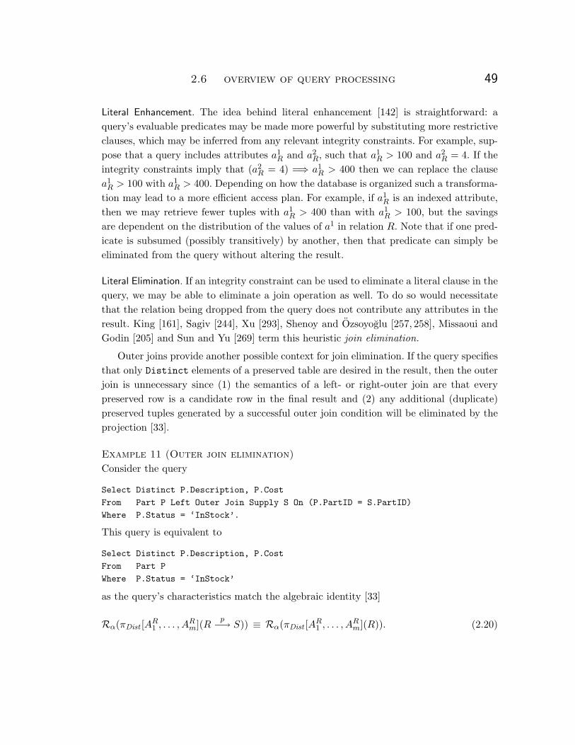
2.6 overview of query processing 49
Literal Enhancement. The idea behind literal enhancement [142] is straightforward: aquery’s evaluable predicates may be made more powerful by substituting more restrictiveclauses, which may be inferred from any relevant integrity constraints. For example, sup-pose that a query includes attributes a1
R and a2R, such that a
1R > 100 and a2
R = 4. If theintegrity constraints imply that (a2
R = 4) =⇒ a1R > 400 then we can replace the clause
a1R > 100 with a1
R > 400. Depending on how the database is organized such a transforma-tion may lead to a more efficient access plan. For example, if a1
R is an indexed attribute,then we may retrieve fewer tuples with a1
R > 400 than with a1R > 100, but the savings
are dependent on the distribution of the values of a1 in relation R. Note that if one pred-icate is subsumed (possibly transitively) by another, then that predicate can simply beeliminated from the query without altering the result.
Literal Elimination. If an integrity constraint can be used to eliminate a literal clause in thequery, we may be able to eliminate a join operation as well. To do so would necessitatethat the relation being dropped from the query does not contribute any attributes in theresult. King [161], Sagiv [244], Xu [293], Shenoy and Ozsoyoglu [257, 258], Missaoui andGodin [205] and Sun and Yu [269] term this heuristic join elimination.
Outer joins provide another possible context for join elimination. If the query specifiesthat only Distinct elements of a preserved table are desired in the result, then the outerjoin is unnecessary since (1) the semantics of a left- or right-outer join are that everypreserved row is a candidate row in the final result and (2) any additional (duplicate)preserved tuples generated by a successful outer join condition will be eliminated by theprojection [33].
Example 11 (Outer join elimination)
Consider the query
Select Distinct P.Description, P.Cost
From Part P Left Outer Join Supply S On (P.PartID = S.PartID)
Where P.Status = ‘InStock’.
This query is equivalent to
Select Distinct P.Description, P.Cost
From Part P
Where P.Status = ‘InStock’
as the query’s characteristics match the algebraic identity [33]
Rα(πDist [AR1 , . . . , A
Rm](R
p−→ S)) ≡ Rα(πDist [AR1 , . . . , A
Rm](R)). (2.20)

50 preliminaries
Restriction Introduction. The idea behind this heuristic is to reduce the number of tuplesthat require retrieval by introducing additional (conjunctive) predicates which the queryoptimizer can exploit as matching index predicates. This technique is also referred to asscan reduction by King [160] and Shenoy and Ozsoyoglu [258].
Generating the transitive closure of any equality conditions specified in the originalquery is one way of introducing additional predicates [165, 221]. Care must be taken to en-sure that the query optimizer takes into account the fact that the additional predicatesare not independent from the others and are redundant in the sense that they do not af-fect the query’s overall result. Hence the selectivities of these redundant predicates mustnot be ‘double counted’. Integrity constraints provide another source of additional pred-icates, though as mentioned previously Check constraints in ansi sql must be suitablymodified to take into account the existence of null values.
Restriction introduction also encompasses the technique of predicate move-around[181] which generalizes classical predicate pushdown [263] by utilizing functional depen-dencies to move predicates up, down, and ‘sideways’ in an expression tree.
Join Introduction. Here, the heuristic attempts to reduce the number of tuples involvedoverall by introducing another relation into the query that contributes no attributes tothe result. If the new relation’s relative size is substantially smaller than the other rela-tion(s) involved, executing the join may be less costly than proceeding with the originalquery. Chakravarthy, Grant, and Minker [50] call the technique literal introduction sincea predicate must be introduced into the query to represent the join.
Index Introduction. Index introduction [161] tries to use an integrity constraint that refersto both a query-restricted attribute, and another attribute in the same relation that is in-dexed. With this transformation the optimizer can reduce the query cost from a possi-ble sequential scan to a series of probes using the index. If the index is clustered then thefinal cost will be further reduced. Note the linking of this heuristic to the physical im-plementation of the supporting data structure: it is not clear that query transformationscan be made entirely independent from the choice of the underlying physical system.
Result by Transformations. This approach, by Chakravarthy et al. [50], is a hybrid of theheuristics discussed above. The idea is as follows. The set of integrity constraints for thedatabase may include implication constraints, such as ‘Chicago ships only red parts’. Aquery which asks ‘What color parts are shipped from Chicago?’ may then be answeredsolely on the knowledge contained within the constraints. In this case, no database accessis required.

2.6 overview of query processing 51
Another situation may involve referential integrity constraints. It may be possibleto determine that if the database contains a tuple, or set of tuples, meeting certain con-straints, then the answer to the query must correspond to the existence, or non-existence,of a particular tuple in the database. Although this result must be verified by a lookupto the actual database, such a lookup is probably much preferable to executing the orig-inal query.
Result by Contradiction. This method is not a heuristic per se. During the query transfor-mation stage we may arrive at a contradiction between the integrity constraints of thedatabase and the query predicates (though in general this problem is undecidable). Sucha contradiction implies an empty result, and therefore we require no database access toanswer the query.
2.6.2.2 Algebraic transformations
View expansion and merging. Typically, an initial phase of algebraic rewriting involvesview expansion and view merging. In view expansion, any views referenced in a Select
block are expanded from their definition stored in the database catalog. View merging at-tempts, where possible, to merge the view directly into the query so as to standardizethe query’s internal representation in a canonical form that minimizes any differences be-tween a query that references a view and one that directly references the view’s underly-ing base tables [71, 186].
Example 12
Consider the query
Select C.Name, C.Address
From Canadian-Suppliers C, Supplier-Summary S
Where C.VendorID = S.VendorID and
S.AverageCost > 50.0
which retrieves those Canadian vendors who, on average, supply relatively expensiveparts. Suppose that the view canadian-suppliers is defined as
Select V.VendorID, V.Name, V.Address
From Vendor V
Where V.Address like ‘%Canada%’
and the grouped view supplier-summary is defined as
Select S.VendorID, Count(*), Avg(P.Cost) as AverageCost
From Parts P Join Supply S On ( P.PartID = S.PartID)
Group by S.VendorID.

52 preliminaries
Π
σ
Project C.Name, C.Address
Restrict on AverageCost
CanadianSuppliers
SupplierSummary
Join on VendorID
Figure 2.4: An expression tree embodying a syntactic mapping for the query in Exam-ple 12.
Figure 2.4 illustrates a syntactic mapping of this query into a relational algebra expres-sion tree.
During the view expansion step, the view definitions stored in the system’s catalog re-place the view references in the original query (see Figure 2.5). For the query in Exam-ple 12, the expression tree now contains three projection nodes that correspond to thethree Select blocks present in the original query and the two referenced views. A crit-ical part of the view expansion process is keeping track of the aliases and correlationnames used in the query or any referenced view. For example, both the query and oneor more referenced views may refer to the same or different schema objects by the samename; during view expansion care must be taken not to confuse the different instances ofthe referenced objects.
Once the views have been expanded, a subsequent step is to merge (where possi-ble) the view definition with its referencing query block (see Figure 2.6). The goal of thisrewriting is to produce a tree in canonical form with superfluous projection operations

2.6 overview of query processing 53
Π
σRestrict onVendor address
Join on P.PartID = S.PartIDVendor
Part Supply
Π P
G
Project V.VendorID, V.Name, V.Address
σ
Group (partition) onS.VendorID
Group-by Project onS.VendorID, Count(*),Avg(P.Cost)
Restrict on AverageCost
Join on VendorID
Project V.Name, V.Address
Figure 2.5: An expression tree containing expanded view definitions for the query inExample 12.
removed. As mentioned previously, view reference information is often kept as ‘annota-tions’ to the expression tree in case subsequent cursor operations refer to a view.
In most commercial systems an initial rewriting is restricted to select-project-joinviews (often termed spj-expressions)14. Views that contain Distinct, Group by, or anyof the set operators Union, Intersect, or Except remain as is until other more com-plex rewritings are performed (see below). In general, spj views can be merged becausetheir algebraic operations (restriction, projection, join, and Cartesian product) both com-
14 Other rewritings of more complex expressions are possible; for example, several systems utilizemagic sets rewriting [209, 210, 253, 254, 278] of grouping, aggregation, and distinct projectionoperations. These other semantic optimizations usually take place after view expansion andmerging.

54 preliminaries
Π
σRestrict onVendor address
Join on P.PartID = S.PartID
Vendor
Part Supply
P
G
σ
Group (partition) onS.VendorID
Group-by Project onS.VendorID, Count(*),Avg(P.Cost)
Restrict on AverageCost
Join on VendorID
Project V.Name, V.Address
Figure 2.6: An expression tree containing expanded view definitions, with one mergedspj view, for the query in Example 12.
mute and associate with the expressions in the referencing query block (cf. Maier [193,pp. 302–4] and Ullman [278]). In particular, it is the following algebraic identity [278,pp. 665]
Rα(πAll [A1R, . . . , A
nR](σ[C](e))) (2.21)
is equivalent to
Rα(πAll [A1R . . . , A
nR](σ[C](πAll [A1
R, . . . , AnR](e)))),
where e is any algebraic expression, that enables the merging of spj views.

2.6 overview of query processing 55
Many systems include the various outer join operators as part of the class of opera-tions that constitute spj expressions. Well-known axioms for the associativity and com-mutativity of outer joins have been previously published (cf. Galindo-Legaria and Rosen-thal [98]). However, almost without exception these axioms fail to consider the impactof an outer join on the projection operator. Identity (2.21) above, originally defined forclassical relational algebra, fails to hold when e can contain any form of outer join. Theproblem lies with the semantics of outer join which generates an all-Null row for thenull-supplying side should the join condition not evaluate to True for at least one pre-served row.
Example 13 (Projection and outer join)
Consider the query
Select P.PartID, P.Description, V.Rating′
From Part P Left Outer Join
( Select S.PartID, f( S.Rating ) as Rating′ From Supply S ) as V
On ( P.PartID = V.PartID )
which will generate a Null value for Rating′ for a part that is not supplied by any sup-plier. This query is not equivalent to the rewritten query
Select P.PartID, P.Description, f( S.Rating )
From Part P Left Outer Join Supply S
On ( P.PartID = S.PartID )
if the scalar function f can evaluate to a definite value when its argument is Null. ansisql functions that have this property include Nullif, Case and Coalesce. More for-mally,
Rα(πAll [f(AmT )](R ✶ (πAll [f(Am
T )](SC1−→ T )))) (2.22)
is not equivalent to
Rα(πAll [f(AmT )](R ✶ (S C1−→ T )))
if f() can evaluate to a definite value when any of its arguments are Null.
More complex algebraic transformations, such as the rewriting of nested queries asjoins [157], involve detailed analysis of the query’s semantics, any integrity constraints im-posed by the schema, and the application of axioms that hold for the various algebraic op-erations. It is beyond the scope of this thesis to exhaustively document the rewrite trans-formations that have been proposed. Herein we present a sampling of semantic transfor-mations that have appeared in the literature, with a focus towards their exploitation offunctional dependencies (if any).

56 preliminaries
Elimination of unnecessary Distinct processing. Since duplicate elimination is typically im-plemented through either sorting or hashing the entire input, it pays to eliminate unnec-essary duplicate elimination whenever possible [228, 230, 281]. Because duplicate elimina-tion is unnecessary when the projection contains a key, the sufficient condition to avoid aredundant sort is to discover if the derived table given by the query contains a key. This isdone by exploiting schema constraints (e.g. primary key declarations) and utilizing func-tional dependencies implied by conjunctive conditions in the query’s Where clause.
Transformations that exploit associativity and commutativity of operators. Join order enu-meration relies on the associativity of Cartesian product and inner joins and the com-mutativity of restriction with both these operators to arrive at an optimal access plan.However, one can transform a query during query rewriting by exploiting axioms thathold for each specific operator. For example, it is common for an optimizer to rewrite anouter join as an inner join when there exists a conjunctive, null-intolerant predicate on anull-supplying table in a Where or Having clause [94, 98]. Galindo-Legaria [98] offers ad-ditional outer join transformations that can assist an optimizer by giving it more flexibil-ity in choosing the query’s join strategy. To this end, various researchers [31, 74, 235, 237]have proposed a generalized join operator that is ‘re-orderable’; input queries are then re-cast using this generalized join operator, whose semantics are fully understood by therest of the optimizer.
Subquery unnesting and magic sets. Kim [157, 158] originally suggested rewriting corre-lated, nested queries as joins to avoid nested-loop execution strategies; his desired ‘canon-ical form’ was n − 1 joins for a query over n relations. Subsequently, several researcherscorrected and extended Kim’s work, particularly in the aspects of grouping and aggre-gation [47, 74, 101, 155, 188, 212, 213, 228, 230, 288]. Pirahesh, Hellerstein, and Hasan [230]document the implementation of these transformations in starburst. As with unneces-sary duplicate elimination, several of the rewriting techniques for nested queries rely onthe discovery of derived key dependencies, exploiting any functional dependencies thatcan be inferred from query predicates.
starburst and its production version, db2 Common Server, implement these trans-formations using a rule-based implementation where the transformation is expressed asa condition-action pair [231]. Magic set optimization techniques [209, 210, 253, 254] aremore complex methods to unnest subqueries that contain grouping and aggregation byfirst materializing intermediate results that are subsequently joined with components ofthe original query to produce an equivalent result.
Common subexpression elimination. Hall [122] proposed simplifying common subexpres-sions in the prtv system to eliminate the unnecessary query processing cost of evaluating
2.6 overview of query processing 57
redundant expressions. Jarke [144] pursues this idea in the context of multiple query opti-mization; Aho et al. [7] and Sagiv [244] exploit simplification rules for conjunctive queriesto minimize the number of rows in tableaux, thereby minimizing the number of joins.
Eager and lazy aggregation. Yan and Larson [294–296], Chaudhuri and Shim [54, 55, 57],and Gupta et al. [117] have independently studied the problem of group-by pullup/push-down: that is, rewrite transformations that ‘pull’ a group-by operation past a join inan algebraic expression tree, or its converse, group-by pushdown. In both cases, the op-timization is based upon the discovery of derived key dependencies; this discovery uti-lizes declared key dependencies, functional dependencies inferred from predicates, andother schema constraints. This is similar to the situation in discovering unnecessary du-plicate elimination for spj queries, but made more complex due to the introduction ofthe group-by and aggregation operators.
A difficult problem with group-by pullup/pushdown is that it can exponentially in-crease the size of the optimization problem. Moreover, as Yan has shown [294], not all ofthe various possible rewritings for a given query may offer improved performance, whichChaudhuri and Shim [55] claim cannot be analyzed by comparing execution plan sub-trees in isolation. One reason for this is that the placement of a Group by node can affectthe plan’s interesting orders [247, 261] and can thus affect the optimization and perfor-mance of the other plan operators. These complexities have led to research on cost-basedcomparison of rewrite alternatives [55, 57, 253] and/or some gross restrictions on the strat-egy space considered [55, 57].
Materialized views. Adiba and Lindsay [5, 6] originally proposed the use of materializedviews to speed query processing by storing precomputed intermediate results redundantly.Semantic query optimization involving such views involves rewriting portions of the queryto reference a materialized view, rather than one or more base tables [52, 53, 174, 175, 297].Larson and Yang [175] separate the complexities of rewriting from optimization; that is,one should only consider rewritten queries that are semantically equivalent to the original.The main aspect of this semantic equivalence is query containment [8, 139, 145, 234, 245]which Larson and Yang specify as the conditions of tuple coverage, tuple selectability, andattribute coverage. Whether or not these conditions hold for one or more materializedviews is in general a pspace-complete problem, since it involves the analysis of quanti-fied Boolean expressions [102, pp. 171–2]. Hence the consideration of strategies that in-volve materialized views significantly increases the overall complexity of the optimizationproblem [1, 52, 53], which, as in the case of multiple query optimization (cf. references[9, 38, 248, 251, 252, 259]) requires common subexpression analysis [10, 59, 89, 144, 227].

58 preliminaries
Functional dependencies are critical to the optimization of queries over materializedviews [26]. For example, consider a materialized view definition consisting of the groupedquery given in Example 1:
Select P.PartID, P.Description, Avg(Q.UnitPrice)
From Part P, Quote Q
Where Q.PartID = P.PartID
Group by P.PartID, P.Description
Now suppose a query over the database is similar in structure to the above, but fails toreference the column P.Description. Such a query is answerable using the view alone,since (1) the view covers all the necessary attributes and (2) the functional dependencyP.PartID −→ P.Description holds. In the converse case—where the query refers to ad-ditional attributes of the part table that are not contained in the view—the existence ofthe functional dependency (in this case, a key dependency) enables a back join [175] tothe part table to retrieve any attributes missing in the view [26].
In a data warehouse environment, the existence of snapshots [6] that summarize mul-tiple base tables means that not all functional dependencies are derivable from schemaconstraints and query or view predicates alone. oracle 8i, which contains extensive ma-terialized view support [26], recognizes this situation and permits a dba to explicitly de-clare the existence of functional dependencies through the specification of Dimension ob-jects. ‘Dimensions’ were originally introduced to identify dependencies across time-seriesdata types (ie. date −→ month), but they can be used to declare dependencies between at-tributes that oracle’s optimizer can try to utilize when determining the attribute cover-age (in oracle terminology, data sufficiency) of a materialized view. No mechanism ex-ists in oracle to enforce these functional dependency constraints, although a class of de-clared inter-relational dependencies—specifically an inclusion dependency—could be en-forced through a referential integrity constraint.
In other contexts, materialized views have been implemented as ‘indexes’ whose exis-tence can be exploited to reduce the number of page accesses for a given access plan. Var-ious implementations of materialized views have been described as view indexes [239, 241,242], join indexes [190, 220, 238, 279, 280, 292], both in relational and object-oriented con-texts, view caches [240], index caches [249, 250], and access support relations [150–154].
An important related problem to the exploitation of materialized views in query op-timization is the problem of view maintenance—that is, strategies to keep the derivedresult and its base tables synchronized in the face of updates [37, 39, 40, 67, 68, 118–120, 123, 189, 240, 274]. In their survey paper from 1995, Gupta and Mumick [119] statethat comprehensive view maintenance techniques have yet be developed that fully ex-ploit functional dependencies and other forms of data constraints. The support for ex-

2.6 overview of query processing 59
plicit declaration of functional dependencies in oracle 8i [26], through its use of dimen-sions, is a step in this direction. oracle 8i also offers the dba both incremental and bulkmaintenance policies, along with specific controls so that the dba can specify whetheror not back-joins to a view’s underlying base tables are permitted in any resulting ac-cess plan. This feature is important as the database instances represented by the view andthe base table(s) may be different: the base tables may have been updated since the ma-terialized view was last refreshed.
2.6.3 Plan generation
The query’s original internal representation (the algebraic expression tree) generally re-flects the original input—that is, the expression tree is an arbitrary shape. Assumingthe query rewrite phase has converted each semantically equivalent query into an inter-mediate representation (see Figure 2.2), the next step is to generate an optimal execu-tion strategy for each of them. Plan generation involves both the sequencing of opera-tions and the choice of their physical implementation (e.g. sort-merge join, hybrid-hashjoin, nested-loop join, etc.). Hence it is typical for an optimizer to transform the alge-braic expression tree into one that represents the physical operations themselves. Concep-tually, the intermediate representation commonly used for execution strategies is an ex-ecutable algebraic expression [51, 226] where each leaf node is a relation in the database,and a nonleaf node is an intermediate relation produced by a physical algebraic opera-tion.
Moreover, a transformation from the original ‘bushy’ algebraic representation to onemore amenable to optimization is often necessary. It is typical for query optimizers—suchas system r [247]—to consider only left-deep processing trees as the solution space forjoin strategy enumeration. For spj queries a left-deep processing tree is one where theright child of any join can only be a base table. For more complex queries, a left-deep treemeans that the right child of any binary operator cannot be a join—though it could bethe (materialized) result of a view containing Union, Group by, or aggregation. Left-deeptrees are desirable because (1) such a tree reduces the need to materialize intermediateresults and (2) the space of ‘bushy’ plans is considerably larger, and hence more expen-sive to search [284]. Ono and Lohman [221] show that the complexity of optimizationalso depends on the number of feasible joins. For example, for a linear query consistingof n tables, a dynamic programming enumeration algorithm must consider (n− 1)2 feasi-ble joins when considering left-deep trees, and (n3 − n)/6 when considering bushy trees.However, for star queries or arbitrary queries containing Cartesian products, the com-plexity is O(3n) or O(4n), depending upon the implementation of the join enumerationalgorithm [229, 284].
60 preliminaries
The objective of plan generation, then, is to [143]:
• generate all reasonable logical access plans corresponding to the desired solutionspace for evaluating the query, and
• augment each access plan with optimization details, such as join methods, physicalaccess paths, and database statistics.
Once the plan generator creates this set of access plans, the plan selection phase willchoose one access plan as the ‘optimal’ plan, using the optimizer’s cost model. Excellentsurveys of join strategy optimization can be found in references [107, 203, 221, 229, 266,284].
Generating an optimal strategy is an np-hard problem [58, 64, 129, 221, 226, 266];to discover all possible strategies requires an exhaustive search. In the worst case, acompletely-connected join graph for a query with n relations has n! alternative strate-gies with left-deep trees, and (2n−2)!
(n−1)! alternatives when considering bushy processing trees[229]. Consequently, optimizers often use heuristics [221, 224, 225, 266] to reduce the num-ber of strategies that the plan selection phase must consider. A common heuristic usedin most commercial optimizers is to restrict the strategy space by performing unaryoperations (particularly restriction) first, thus reducing the size of intermediate results[263, 278]. Another common optimization heuristic, and one used by starburst, is to de-fer the evaluation of any Cartesian products [208] to as late in the strategy as possible[221].
There are several ways to perform join enumeration; a recent paper by Steinbrunn,Moerkotte, and Kemper [266] classifies them into four categories: randomized algorithms,genetic algorithms, deterministic algorithms, and hybrid algorithms. Randomized algo-rithms view solutions as points in a solution space, and the algorithms randomly ‘walk’through this solution space from one point to another using a pre-defined set of moves.Galindo-Legaria, Pellenkoft, and Kersten [96, 99] have recently proposed a probabilis-tic approach to optimization that randomly ‘probes’ the space of all valid join strategiesin an attempt to quickly find a ‘reasonable’ plan, whose cost can then be used to limita deterministic search of the entire strategy space. Other well-known examples of ran-domized approaches include iterative improvement [138, 270, 271] and simulated anneal-ing [140, 271]. Genetic algorithms for join enumeration, such as those described by Ben-nett et al. [27], are very experimental and are derived from algorithms used to analyzegenetic sequences. For example, a left-deep join strategy can be modelled as a chromo-some with an ordered set of genes that represent each table in the join. Join enumerationis performed through randomly ‘mutating’ the genes, swapping the order of two adjacent

2.6 overview of query processing 61
genes, and applying a ‘crossover’ operator, that interchanges two genes in one chromo-some with the corresponding genes in another, retaining their relative order (and, in thiscase, the join implementation method). The latter operator is often described as ‘breed-ing’ since it generates a new chromosome from its two ‘parents’.
Several deterministic join enumeration algorithms have appeared in the literature. in-gres uses a dynamic optimization algorithm [165, 291] that recursively breaks up a calcu-lus (quel) query into smaller pieces by decomposing queries over multiple relations intoa sequence of queries having one relation (tuple variable) in common, using as a basis theestimated cardinality of each. Each single-relation query is optimized by assessing the ac-cess paths and statistical information for that relation in isolation. Ibaraki and Kameda[129] showed that it is possible to compute the optimal join strategy in polynomial time,given certain restrictions on the query graph and properties of the cost model. Krishna-murthy et al. [166] proposed a polynomial-time algorithm that provides an optimal solu-tion, though it can handle only a simplified cost model and is restricted to nested-loopjoins. Swami and Iyer [272] subsequently extended their work in an attempt to removesome of its restrictions, and to also consider access plans containing sort-merge joins.
The best example of a deterministic algorithm is dynamic programming , the ‘classical’join enumeration algorithm used by system r and described by Selinger et al. in theirseminal paper [247]. It performs static query optimization based on exhaustive search ofthe solution space using a modified dynamic programming approach [186, 247]. Originallydeveloped to enumerate only join order, the algorithm has been adapted to handle otheroperators as well: aggregation [57], outer joins [30, 31, 106], and expensive predicates [56,125–127]. The optimizer assigns a cost to every candidate access plan, and retains theone with the lowest cost. In addition, the algorithm keeps track of the ‘sorted-ness’ ofeach intermediate result, which are termed interesting orders [247, 261]. Analysis of theseinteresting orders can lead to less expensive strategies through the avoidance of (usuallyexpensive) sorts on intermediate results.
2.6.3.1 Physical properties of the storage model
To augment equivalent access plans, the plan generator takes into account the physi-cal characteristics of the database. For a join, the optimizer can choose from several joinmethods, such as block nested loop [156], index nested loop, sort-merge, hashed-loop,hybrid-hash, and pid-partitioning [203, 256]. If a query’s selection predicate refers to anindexed attribute, the plan generator may choose to use an indexed retrieval of tuples in-stead of a table scan. It is possible that an index alone may cover the necessary attributesrequired, and hence access to the underlying base table can be avoided [275]. If multi-
62 preliminaries
ple indexes exist, then the generator may choose among them, or create a more sophisti-cated strategy utilizing index intersection and/or index union [207].
For grouped queries, the generator must decide how to best implement the groupingoperation. This is typically done either through sorting or hashing; precisely which tech-niques are used over a given query and data distribution can have a marked effect onquery performance [173]. However, a sort can be avoided if the ordering of tuples from aprevious operation is preserved, e.g. if a table was retrieved using an index [261].
2.6.4 Plan Selection
Selection of an access plan is usually based on a cost model of storage structures andaccess operations [143]. A survey of selectivity and cost estimation is beyond the scopeof this introduction; we refer interested readers to other literature surveys [116, 196, 203].
In centralized query optimizers, some combination of three measures are the basis ofthe cost function that the plan selection phase attempts to minimize:
• working storage requirements; for example, the size of intermediate relations [157,247];
• cpu costs [247]; and
• secondary storage accesses [298].
Most cost models in centralized query optimizers focus primarily on the cost of secondarystorage access, on the basis of estimates of the cardinalities of the operands in the alge-bra tree [73, 247] and a general assumption that tuples are randomly assigned pages insecondary storage [298].
Figure 2.2 illustrates plan selection as a separate phase from plan generation. Withthis approach, an estimated cost is computed for each access plan and the choice of strat-egy is based simply on the one with minimum cost [186, 247, 298]. There are, however,several alternative and complementary approaches. An optimizer can incrementally com-pute the cost of access plans in parallel to their generation. For example, Rosenthal andReiner [236] propose that an optimizer retain only the least expensive strategy to ob-tain an intermediate result, discarding any other approach as soon as its cost exceeds thecheapest one found so far. This technique is used by both oracle [26] and db2 [221] toquickly reduce the number of alternatives so as to minimize the overhead of optimization.Dynamic query optimization is the process of generating strategies only as needed dur-ing execution time, when the exact sizes of intermediate results are known [11, 12, 143].

2.6 overview of query processing 63
The tradeoff in this approach is the generation of a more optimal strategy on the ba-sis of real costs (not estimates) versus the optimization overhead, which now occurs atrun time.
Knowledge of functional dependencies can be useful in cost estimation, but exploit-ing them fully has yet to be studied in detail. For the most part, database systems treatattributes and predicates as independent variables to minimize the complexity of estima-tion [62, 63]. However, several examples of query rewrite optimization described above,such as literal enhancement, clearly can have an impact on the selectivity of a given setof predicates, and hence affect the cost of the overall query.
Several ways to exploit attribute correlations—possibly defined by the existence of oneor more functional dependencies—in cost or selectivity estimation exist in the literature.Bell, Ling, and McClean [25] study techniques to estimate join sizes where known corre-lations exist. Similarly, Vander Zanden et al. [285] explore estimation formulae for blockaccesses when attributes are highly correlated. Wang et al. [289] study several classes ofpredicates whose selectivity are largely affected by correlated attributes. Christodoulakis[60–63] provides additional background on the problems of cost estimation in the face ofattribute correlation.
2.6.5 Summary
Our brief overview of query processing in centralized relational environments is intendedto highlight areas where knowledge of functional dependencies can be exploited. As wehave seen, semantic query optimization, as exemplified by oracle’s support for rewriteoptimization over materialized views, offers significant potential for dramatic reductionsin query execution cost. Nonetheless, specific areas in the plan generation and plan se-lection phases also can benefit from the knowledge of dependencies. In the next chap-ter, we present an algorithm that computes the set of functional dependencies that holdfor a given algebraic expression tree. In Chapters 4 and 5 we look at two ways to ex-ploit these dependencies: techniques for query rewrite optimization, and the interactionof functional dependencies with interesting orders.


3 Functional dependencies and query decomposition
In this chapter we present algorithms for determining which interesting functional de-pendencies hold in derived relations (we discuss what defines an interesting dependencyin the first section). In particular, for each relational algebra operator (projection, selec-tion, etc.) we give an algorithm to compute the set of interesting dependencies that holdon output, given the set of dependencies that hold for its inputs. Our contributions are:
1. we analyze a wider set of algebraic operators (including left- and full outer join)than did Darwen [70] or Klug [162], and in addition consider the implications ofnull values and sql2 semantics;
2. the algorithm handles the specification of unique constraints, primary and candi-date keys, nullable columns, table and column constraints, and complex search con-ditions to support the computation of derived functional dependencies for a reason-ably large class of sql queries; and
3. we formally prove the correctness of our results.
Our representation of functional dependencies, described in Section 3.3, uses an extendedform of fd-graphs previously introduced by Ausiello, D’Atri , and Sacca [19]. fd-graphsare a specialized form of directed hypergraph. In an fd-graph, a vertex represents a single-ton attribute, and directed edges represent functional dependencies. A hypervertex rep-resents composite determinants which consist of more than one attribute. Ausiello et al.claim that fd-graphs offer a more natural basis for formal analysis of functional depen-dencies than other approaches, such as Bernstein’s [28] derivation trees. Our extensions tofd-graphs are required to represent derived dependencies in ansi sql expressions, whichcan include outer joins, null values and three-valued logic, and multiset semantics.
The rest of the chapter is organized as follows. After some preliminary discussion ofsources of dependency information inherent in relational expressions, in Section 3.2 weprovide the theoretical foundation for the determination of strict functional dependen-cies, lax functional dependencies, and strict and lax equivalence constraints for an arbi-trary relational expression e consisting of the relational algebra operators introduced in
65

66 functional dependencies and query decomposition
Section 2.3. We will utilize the virtual attributes of extended tables to enable the deriva-tion of transitive dependencies over attributes that have been projected out of an inter-mediate or final result. We reiterate that our definition of extended table provides onlya proof mechanism; their implementation is unnecessary. Section 3.4, which contains thischapter’s main contributions, presents algorithms to develop an fd-graph for an arbi-trary relational expression e that represents those derived functional dependencies thathold in e. Once constructed, the fd-graph can be analyzed for dependencies that can af-fect the outcomes of semantic query optimization algorithms, as described in Chapter 4,or can affect the outcome of sort avoidance analysis, as described in Chapter 5. In Sec-tion 3.5 we formally prove the correctness of the fd-graph construction algorithms. Sec-tion 3.6 describes and proves algorithms to compute dependency and equivalence closuresfrom an fd-graph. Section 3.7 briefly summarizes known work in exploiting functional de-pendencies in query optimization, and finally Section 3.8 concludes with some ideas forfurther research.
3.1 Sources of dependency information
As described in Chapter 2, relational database systems typically represent a query, orrelational expression e, as an algebraic expression tree. Derived functional dependenciesresult from the semantics of the various unary and binary relational algebra operatorssuch as projection, selection, and join that make up the expression (see Figure 2.3). InSection 3.2 below we will describe in detail the functional dependencies implied by each ofthe algebraic operators. But before we do so, we outline the broad categories of semanticinformation inherent in schema definitions and algebraic expressions that can be analyzedto infer derived functional dependencies.
3.1.1 Axiom system for strict and lax dependencies
Sources of additional dependencies include the axiom system for strict and lax dependen-cies defined in Section 2.5.2. A trivial example of a strict transitive dependency is the log-ical implication of A −→ C from the two strict functional dependencies A −→ B andB −→ C (through the application of inference rule fd7a, strict transitivity). More for-mally, a set of strict functional dependencies F implies a strict dependency f if f holdsin every extended table in which F holds.
Definition 30 (Strict dependency closure)
The strict closure of F , denoted−→F+, is the set of all strict functional dependencies logi-
cally implied by F through application of the axioms defined in Section 2.5.2. The strict

3.1 sources of dependency information 67
closure of a set of attributes X with respect to F , denoted−→X+
F , is the set of attributesfunctionally determined by X through direct or transitive strict dependencies defined by
the strict closure of F . That is,−→X+
F= {A | X −→ A ∈−→F+}.
It is easy to see that the number of dependencies in−→F+ is exponential in the size
of the universe of attributes and the given set F [24], due in part to the reflexivity ax-iom (e.g. if Y ⊆ X we have X −→ Y ). These dependencies are ‘uninteresting’ in the sensethat they convey no useful information about the constraints that hold in either a de-rived or a base table. We explicitly avoid the exponential explosion of representing suchtransitive dependencies by keeping F in a simplified form.
Definition 31 (Simplified form)
A set of dependencies F is in simplified form [79] if the following conditions hold:
1. for all dependencies f ∈ F , X −→ Y =⇒ (X ∩ Y ) = ∅.
2. F contains no duplicate dependencies with identical left- and right-hand sides.
Furthermore, we assume that all strict and lax functional dependencies in F have singleattribute dependents (right-hand sides)15.
Definition 32 (Lax dependency closure)
Similarly to strict closure, the lax closure of F , denoted�−→F+, is the set of all lax func-
tional dependencies logically implied by F through application of the axioms defined in
Section 2.5.2. The lax closure of a set of attributes X with respect to F , denoted�−→X+
F ,is the set of attributes functionally determined by X through direct or transitive lax de-
pendencies defined by the lax closure of F . That is,�−→X+
F= {A | X &−→ A ∈�−→F+}.
For convenience we denote the union of the closures of the set of strict and lax functionaldependencies in F with the notation F+ =
−→F+ ∪
�−→F+. We avoid the exponential explosion
of lax transitive dependencies by also maintaining the lax functional dependencies in Fin simplified form.
15 Note that lax decomposition only holds in the case of definite attributes (rule fd4b).

68 functional dependencies and query decomposition
3.1.2 Primary keys and other table constraints
Schema constraints, such as primary keys, unique indexes, and unique constraints formthe basis of a known set of strict or lax functional dependencies that are guaranteed tohold for every instance of the database. However, because we intend to maintain onlynon-trivial dependencies in simplified form, F will not contain any dependencies betweenan attribute and itself. Consider, however, an sql table T consisting of the single columnAT = {a1} that cannot contain duplicate rows—that is, a1 is a primary key of T . Thisuniqueness cannot be represented in F if we restrict dependencies to attributes in T .
To solve this problem we utilize the unique tuple identifier attribute ι(R) in the ex-tended table R (see Section 2.2 above). ι(R) is the dependent attribute of each key depen-dency, and is the determinant of a set of strict dependencies whose dependent attributesare in the set α(R)∪ρ(R). For sql base tables, this mechanism provides a source of func-tional dependencies even for those tables that have various forms of unique constraintsbut lack a primary key.
3.1.3 Equality conditions
Observe that if a particular attribute X ∈ sch(R) is guaranteed to have the same valuefor each tuple in I(R), then in F+ all attributes in sch(R) functionally determine X.This is typical for derived tables formed by restriction, when the query includes a Where
clause that contains an equality condition between a column and a constant. For queryoptimization purposes it would be a mistake to lose the circumstances behind the gener-ation of this new set of dependencies; knowing that an attribute is equated to a constantcan be exploited in a myriad of ways during query processing, in particular the satisfac-tion of order properties [261] (see Chapter 5).
Further observe that an equality condition in a false-interpreted Where clause predi-cate, e.g. A = B, will correspond to the two strict functional dependencies A −→ B andB −→ A in F . However, in this case, as in the one above, it is important to retain thefact that these dependencies stem from equalities, and that not only do the dependen-cies hold but that one attribute (or constant) can be substituted for the other becausetheir values are the same. Henceforth we denote the set of strict attribute equivalenceconstraints that exist in an expression e using the symbol E .

3.1 sources of dependency information 69
Definition 33 (Strict equivalence constraint)
Consider an extended table R and singleton attributes A1 ⊆ sch(R) and A2 ⊆ sch(R)where A1 �= A2. Let I(R) denote a specific instance of R. Then A1 is strictly equivalent
to A2 in I(R) (written A1
I(R)ω= A2) if the following condition holds:
∀ t0 ∈ I(R) : t0[A1]ω= t0[A2]. (3.1)
Claim 14 (Inference axioms for strict equivalence constraints)
The inference rules:
Identity eq1 Xω= X.
Strict commutativity eq2 If X ω= Y then Yω= X.
Strict transitivity eq3 If X ω= Y and Yω= Z then X
ω= Z.Strict implication eq4 If X ω= Y then X −→ Y and Y −→ X.
defined over an instance I(R) of an extended table R with singleton attributes X,Y, Z ⊆sch(R) are sound.
Conjunctive equality conditions between attribute pairs in an outer join’s On conditioncan, in some circumstances, produce a result where the attribute pair has identical val-ues except for a result row that contains an all-Null row generated for the null-supplyingside. We term this weak form of attribute equivalence a lax equivalence constraint.
Definition 34 (Lax equivalence constraint)
Consider an extended table R and singleton attributes A1 ⊆ sch(R) and A2 ⊆ sch(R)where A1 �= A2. Let I(R) denote a specific instance of R. Then A1 is laxly equivalent to
A2 in I(R) (written A1I(R)) A2) if the following condition holds:
∀ t0 ∈ I(R) : �t0[A1] = t0[A2]�. (3.2)
Again we write A1 ) A2 when I(R) is clear from the context. Henceforth when we use theterm ‘equivalence constraint’ without qualification we mean either a strict or lax equiv-alence constraint.
Lemma 4 (Inference axioms for lax equivalence constraints)
The inference rules:
Lax commutativity eq5 If X ) Y then Y ) X.Weakening eq6 If X ω= Y then X ) Y .Strengthening eq7 If X ) Y and I(R) is XY -definite then X
ω= Y .Lax implication eq8 If X ) Y then X &−→ Y and Y &−→ X.
defined over an instance I(R) of an extended table R with singleton attributes X,Y ⊆sch(R) are sound for a combined set of strict and lax equivalence constraints.

70 functional dependencies and query decomposition
Proof. Omitted. ✷
By Claim 14, strict equivalence constraints are transitive; if X ω= Y and Yω= Z then
Xω= Z, which corresponds to our definition of functional dependencies (Definition 26).
However, like lax functional dependencies (Definition 28 on page 36), lax equivalence con-straints are transitive only over definite attributes.
Lemma 5 (Transitivity of lax equivalence)
The inference rules
Lax transitivity eq9a If X ω= Y and Y ) Z then X ) Z.eq9b If X ) Y and Y ) Z and I(R) is Y -definite then X ) Z.
defined over an instance I(R) of an extended table R with singleton attributes X,Y, Z ⊆sch(R) are sound for a combined set of strict and lax equivalence constraints.
Proof (Rule EQ9a). We first consider rule eq9a. Consider an instance I(R) of ex-tended table R. By contradiction, assume that rule eq9a is not sound. Then we musthave X ω= Y and Y ) Z, but X �) Z. If X �) Z then there must exist at least one tu-ple, say r0 in I(R), that has different X- and Z-values that are each not Null. However,since X ω= Y , r0 must have identical definite X- and Y -values. Since Y ) Z holds and r0must have definite Y - and Z-values, then we must have r0[X] = r0[Y ] = r0[Z], a contra-diction. ✷
Proof (Rule EQ9b). Consider an instance I(R) of an extended table R where at-tribute Y ⊂ sch(R) is definite. By contradiction, assume that rule eq9b is not sound.Then we must have X ) Y and Y ) Z, but X �) Z. If X �) Z then there must ex-ist at least one tuple, say r0 in I(R), that has different X- and Z-values that are each notNull. However, since X ) Y and r0[Y ] is definite, then we must have r0[X] = r0[Y ]. Sim-ilarly, r0[Y ] = r0[Z], which implies that r0[X] = r0[Z]; a contradiction. Hence rule eq9bis sound. ✷
Theorem 2 (Inference rules for equivalence constraints)
The inference rules eq1 through eq9 are sound for a combined set of strict and lax equiv-alence constraints.
Proof. Follows from Claim 14, Lemma 4, and Lemma 5. ✷

3.2 dependencies implied by sql expressions 71
Definition 35 (Strict equivalence closure)
The strict equivalence closure of E , denoted E+, is the set of all equivalence constraintslogically implied by E through the application of the axioms defined in Claim 14. Thestrict equivalence closure of an attribute X with respect to E , denoted X+
E , is the equiv-alence class of X such that all elements in the set are guaranteed to have the same valuefor any tuple t in an instance I(R). That is, X+
E = {A | X ω= A ∈ E+}.
Definition 36 (Lax equivalence closure)
The lax equivalence closure of E , denoted E+, is the set of all equivalence constraintslogically implied by E through the application of the axioms defined in Claim 14 andLemmas 4 and 5. The lax equivalence closure of an attribute X with respect to E , denotedX+
E , is the equivalence class of X such that all elements in the set are guaranteed to havethe same value for any tuple t in an instance I(R), or may be Null. That is, X+
E = {A |X ) A ∈ E+}.
For convenience, we denote the union of the strict and lax equivalence closures of aset of equivalence constraints E with the notation E+ = E+ ∪ E+.
3.1.4 Scalar functions
A source of additional dependencies stems from the presence of scalar functions andarithmetic expressions (which we assume to be deterministic and free of side-effects) ina query’s Select list or one of its clauses. In Example 3 on page 8 we introduced scalarfunctions using the following example query:
Select P.*, (P.Price - P.Cost) as Margin
From Part P
Where P.Status = ‘InStock’.
One can consider Margin as the result of a function whose input parameters areP.Price and P.Cost. In this case the derived strict functional dependency { P.Price,
P.Cost } −→ Margin holds in the result. We arbitrarily assume that the result of anysuch computation is possibly Null.
3.2 Dependencies implied by SQL expressions
While determining the dependencies that hold in the final query result can be benefi-cial, clearly such information can be exploited during the query optimization process foreach subtree (including nested query blocks) of the complete algebraic expression tree.Below we describe a large class of strict and lax functional dependencies that are im-plied by each algebraic operator. To determine the set of dependencies that hold in an

72 functional dependencies and query decomposition
entire expression e, one can simply recursively traverse the expression tree in a postfixmanner and compute the dependencies that hold for a given operator once the dependen-cies of its inputs have been determined.
As most database systems directly implement existential quantification (and do notimplement relational division—see Graefe and Cole [109]) the algebraic expression treee that represents an ansi sql query expression also includes (possibly negated) Existspredicates that refer to correlated or non-correlated [188] subqueries. We use this combi-nation calculus-algebra expression tree as the basis for forming an internal representationof a query (or sub-query) and manipulate this internal representation during query opti-mization to derive a more efficient computation of the desired result [90, 110, 111, 247].
If we assume that all forms of nested query predicates in sql (Any, All, In, etc.)have been rewritten as Exists predicates (see Section 2.3.1.2) then a bottom-up analysisof the subqueries can treat any correlation attributes from super-queries as constant val-ues. As Exists predicates restrict the result set of a derived table, the handling of thesepredicates is explained as part of the restriction operator in Section 3.2.4 below.
Claim 15 (Dependencies and constraints in SQL tables)
The following statements regarding functional dependencies and equivalence constraintsthat hold for any extended table R over attributes Xyz ⊆ sch(R), where X denotes a setand y and z denote atomic attributes, are true for the corresponding sql table Rα(R):
• If f : X −→ y holds in I(R) and Xy ⊆ α(R) then f holds in the correspondinginstance of Rα(R).
• If f : X &−→ y holds in I(R) and Xy ⊆ α(R) then X &−→ y in the subset of thecorresponding instance of Rα(R) where each of the values of X and y are not Null.
• If f : X −→ y holds in I(R), X ⊆ α(R), and ι(R) = y then X forms a candidate su-perkey of Rα(R): there cannot be two rows in the corresponding instance of Rα(R)that have identical X-values.
• If f : X &−→ y holds in I(R), X ⊆ α(R), and ι(R) = y then there cannot be tworows in the corresponding instance ofRα(R) that have identical non-Null X-values.
• If f : X −→ y holds, y ∈ α(R), and X ⊆ κ(R), then each row of the correspondinginstance of Rα(R) has an identical Y -value (possibly Null).
• If f : X &−→ y holds, y ⊆ α(R), and X ⊆ κ(R), then in each row of the correspond-ing instance of Rα(R) either Y is Null or Y is the identical non-Null value.

3.2 dependencies implied by sql expressions 73
• If e : y ω= z holds in I(R) and yz ⊆ α(R) then each row in Rα(R) contains identical(possibly Null) values for y and z. If either y or z are constants in κ(R), then eachrow in Rα(R) will have a value identical to that of the constant.
• If e : y ) z holds in I(R) and yz ⊆ α(R) then each row in Rα(R) either containsidentical non-Null values for y and z, or at least one of y or z is Null. Similarly, ify is a constant in κ(R) then each row of Rα(R) either contains identical values ofz, equivalent to the value of the constant y, or z is Null.
3.2.1 Base tables
At the leaves of the expression tree are nodes representing quantified range variablesover base tables. The Create Table statement for these tables—see the examples in Ap-pendix A—include declarations of one or more keys (see Section 2.4.1). We do not at-tempt to determine a minimal key, if it exists, for each operator in the tree. In part wedo this because of the complexity of finding one or all of the minimal keys for any alge-braic expression e (cf. Fadous and Forsyth [82], Lucchesi and Osborn [191], and Saiedianand Spencer [246]). We also refrain from computing sets of minimal keys throughout thetree due to the realization that much of the computation will likely be wasted. Often it issufficient to determine the closure of a set of attributes—for example, finding if the clo-sure of a set of attributes includes a key of a base table (see Chapter 4).
Other arbitrary constraints on base tables can be handled as if they constitute a re-striction condition on R (see Section 3.2.4). Since table constraints are true-interpreted(if their value is unknown then the constraint still holds), then those Check constraintsover non-null attributes can imply strict dependencies and/or equivalence constraints ifthe Check constraint includes an equality condition that can be recognized during con-straint analysis (see Section 3.2.4). Otherwise, such constraints may infer a lax depen-dency or equivalence constraint that should still be captured in case the existence of anynull-intolerant restriction predicates can later be used to transform a lax dependency orequivalence constraint into a strict one.
Claim 16 (Dependencies and constraints in base tables)
The set of attributes Ki(R) of the primary key and each unique index on a base tableRα(R) imply strict functional dependencies of the form Ki −→ ι(R) hold in I(R). Simi-larly, the set of attributes Ui(R) of each unique constraint on a base table Rα(R) implylax functional dependencies of the form Ui &−→ ι(R) hold in I(R).

74 functional dependencies and query decomposition
3.2.2 Projection
The primary purpose of the projection operator πAll and the distinct projection oper-ator πDist is to project an extended table R over attributes A, thereby eliminating at-tributes from the result. In the case of πDist , the auxiliary purpose is to eliminate ‘dupli-cate’ tuples from the result with respect to A. Clearly any functional dependency that in-cludes an attribute not in A is rendered meaningless; however, we must be careful not tolose dependencies implied through transitivity. Unlike Darwen’s approach [70], which re-lies on the recomputation of the closure F+ at each step, we intend to compute F+ asseldom as possible. This means that we must maintain dependency information even fora table’s virtual columns (see Section 2.2).
The projection and distinct projection operators can both add and remove functionaldependencies to the set of dependencies that hold in the result. If projection includesthe application of scalar functions, then R is extended with the result of the scalar func-tion to form R′. Moreover, new strict functional dependencies now exist between thefunction result λ and its input(s) (see Section 3.1.4 above). If the projection operator re-moves an attribute, say C, then F+ consists of the closure of the dependencies that holdin the input, less any dependencies that directly include C as a determinant or a depen-dent. In other words, if we have the strict dependencies A −→ ι(R), ι(R) −→ ABCDE,and BC −→ F and attribute C is projected out, then the dependencies ι(R) −→ C andBC −→ F can no longer hold, since attribute C is no longer present. However, by the in-ference axioms presented in Section 2.5.2 the transitive dependency A −→ F still holdsin the extended table formed by e.
Claim 17 (Dependencies implied by projection)
Let R′ denote the result of the algebraic expression πAll [A](R) denoting the projection(retaining duplicates) of the extended table R over A. Suppose that I(R) satisfies a setof functional dependencies F and a set of equivalence constraints E . The set of functionaldependencies and equivalence constraints that hold in I(R′) are as follows:
• The functional dependencies and equivalence constraints that hold in I(R) continueto hold in I(R′).
• For each scalar function λ(X) ∈ A the strict functional dependencies X −→ λ(X)and ι(R′) −→ λ(X) hold in FR′ .
Proof. Omitted. ✷

3.2 dependencies implied by sql expressions 75
Claim 18 (Dependencies implied by distinct projection)
Let R′ denote the result of the algebraic expression πDist [A](R) denoting the distinct pro-jection of R over A. Suppose that I(R) satisfies a set of functional dependencies F and aset of equivalence constraints E . The set of functional dependencies and equivalence con-straints that hold in I(R′) are as follows:
• The functional dependencies and equivalence constraints that hold in I(R) continueto hold in I(R′).
• For each scalar function λ(X) ∈ A the strict functional dependency X −→ λ(X)holds in FR′ .
• The strict functional dependencies A −→ ι(R′) and ι(R′) −→ α(R′) hold in I(R′).
Proof. Recall that by the definition of distinct projection, we nondeterministically se-lect a representative tuple r for each set of tuples in I(R) with matching values of A.Simply removing a tuple from a set has no effect on the functional dependencies or equiv-alence constraints satisfied by that instance; hence if f holds in R then it must followthat f holds in R′. ✷
3.2.3 Cartesian product
The set of dependencies that hold in the result of a Cartesian product is the union ofthose dependencies that hold in the inputs. Klug [162, pp. 266] stated that the Cartesianproduct of two tables S and T does not add any additional dependencies. However, in ad-dition to dependencies involving attributes, we would like to retain knowledge of key de-pendencies that hold in either input, and if they exist derive a key dependency in theresult. The maintenance of key dependencies is critical to the success of the overall algo-rithm, since we are following both Darwen and Klug by modelling inner join as a restric-tion condition over a Cartesian product.
We observe that if we can guarantee that either of the inputs, say I(S), can haveat most one tuple then KT −→ sch(S) ∪ sch(T ). This optimization is omitted from thealgorithm for computing derived dependencies implied by a Cartesian product, which isdescribed in Section 3.4.4 below.
Claim 19 (Dependencies implied by Cartesian product)
Let R′ denote the result of the algebraic expression R′ = S × T denoting the Cartesianproduct of extended tables S and T . Suppose I(S) satisfies the set FS of functional de-pendencies and the set ES of equivalence constraints, and similarly I(T ) satisfies the setFT of functional dependencies and the set ET of equivalence constraints. The set of func-tional dependencies and equivalence constraints that hold in I(R′) are as follows:

76 functional dependencies and query decomposition
• The set of functional dependencies that hold in I(S), and those that hold in I(T ),continue to hold in I(R′).
• The set of equivalence constraints that hold in I(S), and those that hold in I(T ),continue to hold in I(R′).
• The strict functional dependency (ι(S) ∪ ι(T )) −→ ι(R′) holds in I(R′).
• The strict functional dependency ι(R′) −→ ι(S) ∪ ι(T ) holds in I(R′).
Proof. Omitted. ✷
3.2.4 Restriction
The algebraic restriction operator is used for both selection and having clauses; the se-mantics are identical since we model a Having clause as a restriction operator over the re-sult of a grouped table projection, possibly followed by another projection to remove ex-traneous results of aggregate functions (see Example 7). Restriction is one operator thatcan only add strict functional dependencies to F ; it cannot remove any existing strict de-pendencies.
Both Fagin [83] and Nicolas [218] showed that functional dependencies are equivalentto statements in propositional logic; thus if one can transform a Where or Having predi-cate into an implication, then one can derive an additional dependency that will hold inthe result. For example, the constraint “if A < 5 then B = 6 else B = 7” implies the func-tional dependency A −→ B even though no direct relationship between A and B is ex-pressed in the constraint. Consequently, the problem of inferring additional functional de-pendencies from predicates in a Where or Having clause depends entirely on the sophis-tication of the algorithm that translates predicates into their equivalent logic sentences.
A comprehensive study of this problem is beyond the scope of this thesis. Instead, weconsider a simplified set of conditions. In two earlier papers Klug [162, 164] consideredonly conjunctive atomic conditions with equivalence operators, that is conditions of theform (v = c) (which he terms selection) and conditions of the form (v1 = v2) (whichKlug terms restriction) where v, v1, and v2 are columns and c is a constant. For ease ofreference we term a condition of the form (v = c) a Type 1 condition, and a conditionof the form (v1 = v2) a Type 2 condition. Each false-interpreted equivalence conditionof Type 1 or 2 implies both an strict equivalence constraint and two symmetric strictfunctional dependencies.
Darwen [70] argued that one need consider only conjunctive θ-comparisons because ifa search condition is more complex it can be reformulated using the algebraic set oper-ations union, intersection, and difference. However, with ansi sql semantics such query

3.2 dependencies implied by sql expressions 77
reformulation will not work in general due to the possible existence of null values, com-plex predicates, and duplicate tuples. Consequently, for completeness one must considerdisjunctive conditions as an integral part of handling restriction. However, in this thesiswe do not exploit disjunctive conditions for inferring constraints and functional depen-dencies. We also assume that negated conditions have been transformed where possible(cf. Larson and Yang [175]); in particular, that inequalities (e.g. X �= 5) have been trans-formed to the semantically equivalent X < 5 or X > 5. We also assume that the restric-tion conditions can be simplified through their conversion into conjunctive normal form[264, 290] so as to recognize and eliminate redundant expressions and unnecessary dis-junctions. Once these transformations have been performed, we restrict our analysis ofatomic conditions in a Where clause to conjunctive conditions of Type 1 or Type 2.
We note, however, that the algorithms described can be easily extended to captureand maintain additional equivalence constraints and functional dependencies through amore complete analysis of ansi sql semantics. In addition to θ-comparisons between at-tributes and constants there are several additional atomic conditions that can be ex-pressed in ansi sql: is [not] null, like, and θ-comparisons between an attribute orconstant and a subquery. For the purposes of dependency analysis we could exploit theseother conditions as follows:
• is null predicates. We could interpret an is null predicate as equivalent to aType 1 equality condition with a null value which can either return true or false(and not unknown). Negated is null predicates, e.g. X is not null, could alsobe exploited—in this case X is guaranteed to be definite in the result.
• like predicates. In general Like predicates are useless for functional dependencyanalysis due to the presence of wildcards. However, if no wildcards are specified inthe pattern then the Like predicate is equivalent to an equality predicate with thepattern string.
• equality comparison with a subquery. If the subquery is non-correlated it can beevaluated independently of its outer query block; thus if attribute X is equated to asubquery result then X can be equated to a (yet unknown) constant value, possiblynull.
Extension. If we detect a scalar function λ(X) during the analysis of a Where clause, thenas with both projection and distinct projection we add the result of the function to theextended table produced by restriction as a virtual attribute, to retain the (strict) func-tional dependency X −→ λ(X) in F .

78 functional dependencies and query decomposition
Inferring lax equivalences and dependencies. As a result of the conversion of nested queriesto their canonical form, correlation predicates in a subquery’s Where clause may requiretrue-interpretation. Since true interpretation commutes over both disjunction and con-junction (axioms 1 and 3 in Table 2.3), we can infer lax equivalence constraints and laxfunctional dependencies from each Type 1 and Type 2 condition in these predicates.
Conversion of lax equivalences and dependencies. As per ansi sql semantics, by defaultwe assume that each conjunct of the restriction predicate is false-interpreted. Any null-intolerant predicate referencing an attribute X will automatically eliminate any tuplesfrom the result where X is the null value. Hence for any algebraic operator higher in theexpression tree, it can be guaranteed that X cannot be Null, and this can be extended toany other attribute Y that is (transitively) equated to X. Hence any lax equivalence con-straint involving X can be strengthened, using inference rule eq7, into a strict equiva-lence constraint if X is (transitively) equated to another non-Null attribute or constant.Similarly, we can convert any lax dependencies into strict dependencies once we can de-termine that neither the dependent attributes, nor any of its determinant attributes, canbe Null, satisfying inference axiom fd6 (strengthening). In the case of composite deter-minants, we must be able to show that each individual component cannot be Null.
Claim 20 (Dependencies implied by restriction)
Let R′ denote the result of the algebraic expression R′ = σ[C](R) denoting the restric-tion of R by false-interpreted predicate C. Suppose I(R) satisfies the set F of functionaldependencies and the set E of equivalence constraints. The set of functional dependen-cies and equivalence constraints that hold in I(R′) are as follows:
• The set of strict functional dependencies that hold in I(R) continue to hold in I(R′).Similarly, the set of strict equivalence constraints that hold in I(R) continue to holdin I(R′).
• For each lax functional dependency f : X &−→ Y that holds in I(R), if I(R′) is XY -definite then f holds as a strict dependency in I(R′); otherwise f continues to holdas a lax dependency in I(R′).
• For each lax equivalence constraint e : X ) Y that holds in I(R), if I(R′) is XY -definite then e holds as a strict equivalence constraint in I(R′); otherwise e contin-ues to hold as a lax equivalence constraint in I(R′).
• For each scalar function λ(X) ∈ α(C) the strict functional dependencies X −→λ(X) and ι(R′) −→ λ(X) hold in I(R′).
3.2 dependencies implied by sql expressions 79
• Each false-interpreted Type 1 or Type 2 condition of the form X = Y in C impliesthe strict equivalence constraint X ω= Y and the strict functional dependencies f :X −→ Y and g : Y −→ X hold in I(R′).
• Each true-interpreted Type 1 or Type 2 condition of the form X = Y in C im-plies the lax equivalence constraint X ) Y and the lax functional dependenciesf : X &−→ Y and g : Y &−→ X hold in I(R′).
Proof. Omitted. ✷
3.2.5 Intersection
The result R′ of the intersection of two inputs S and T contains either unique instancesof each tuple in I(R′) with respect to the real attributes in sch(R) (in the case of theIntersect operator) or some number of duplicate tuples corresponding to the definitionof Intersect All. In either case, by our definition of the intersection operators ∩Dist
and ∩All (see Section 2.3.2) a tuple q0 can only exist in the result of R′ = S ∩ T if acorresponding image of q0[α(R)] exists in both I(S) and I(T ). Hence I(R′) must satisfythe set of dependencies that hold with respect to the real attributes in both S and T .
Lemma 6 (Strict dependencies implied by intersection)
Consider a query Q consisting of the intersection of two tables S and T
Q = R ∩All S
where each attribute ASi ∈ α(S) is union-compatible with its corresponding attribute
ATi ∈ α(T ). Suppose I(S) satisfies the strict functional dependency f : AS
1 −→ AS2 ∈ FS ,
where AS1 ∪ AS
2 ⊆ α(S). Then the functional dependency f : AQ1 −→ AQ
2 holds in I(Q),where AQ
1 and AQ2 correspond to the input attributes AS
1 and AS2 .
Proof. By contradiction, assume the dependency f : AQ1 −→ AQ
2 does not hold in Q,but its corresponding dependency AS
1 −→ AS2 holds in S. This means that there exist
at least two tuples q0, q′0 in Q such that q0[AQi ]
ω= q′0[AQi ] but q0[A
Qj ] �ω= q′0[A
Qj ]. By the
definition of intersection, any tuple component q0[α(Q)] in Q must exist in both I(S) andI(T ) (the null comparison operator is used so that null value comparisons resulting inunknown are interpreted as true). Hence the result is both a subset of the tuples in I(S),and a subset of the tuples in I(T ). By our initial assumption, this means that there mustexist tuples in S where the strict functional dependency AS
1 −→ AS2 , where (A
S1 ∪AS
2 ) ⊆α(S), cannot hold in S; a contradiction. A similar situation occurs if the dependency isassumed to hold in T . Hence we conclude that if a dependency holds for real attributesin either S or T then it must also hold in Q. ✷

80 functional dependencies and query decomposition
Since the set of dependencies that hold in Rα(Q) is at least the union of those thathold in Rα(S) and Rα(T ) (with attributes appropriately renamed), then the superkeysthat hold in either S or T also hold in Q, as we formally state below.
Corollary 1 (Superkeys implied by intersection)
Consider a query Q consisting of the intersection of two tables S and T
Q = S ∩All T.
All members of the union of the sets of superkeys in α(S) and α(T ) that hold in S andT respectively hold as superkeys in Q.
Proof. Follows directly from Lemma 6 as the set of functional dependencies that holdin Rα(Q) is at least the union of those that hold in Rα(S) and Rα(T ). ✷
Conversion of lax equivalence constraints and lax functional dependencies. We observe that,similarly to strict functional dependencies, any lax functional dependencies, lax equiva-lence constraints, and strict equivalence constraints that hold in I(S) or I(T ) will con-tinue to hold in Q. However, lax dependencies (equivalence constraints) from one of thetwo inputs may be converted to strict dependencies (equivalence constraints) if, by be-ing ‘paired’ with the other extended table, it can now be guaranteed that both the deter-minant and dependent attributes cannot be Null in the result—exactly as was the casefor the restriction operator.
Example 14 (Lax dependencies and Intersection)
Consider the following query expression involving intersection:
Select S.VendorID, S.PartID, S.Lagtime, S.Rating
From Supplier S
Where S.Rating = ‘B’
Intersect All
Select S.VendorID, S.PartID, S.Lagtime, S.Rating
From Supplier S
Where S.Lagtime > :Lagtime
where :Lagtime denotes a host variable. In the result of the intersection, neither Lagtimenor Rating can be Null since the null-intolerant predicates in each query specification’sWhere clause will prevent null values in the result. Hence a hypothetical lax functionaldependency Lagtime &−→ Rating in either input will hold as a strict dependency in theresult.

3.2 dependencies implied by sql expressions 81
Claim 21 (Dependencies implied by intersection)
Let R′ denote the result of the algebraic expression R′ = S ∩All T denoting the inter-section of extended tables S and T . Suppose I(S) satisfies the set FS of functional de-pendencies and the set ES of equivalence constraints, and similarly I(T ) satisfies the setFT of functional dependencies and the set ET of equivalence constraints. The set of func-tional dependencies and equivalence constraints that hold in I(R′) are as follows:
• The set of strict functional dependencies that hold in I(S), and those that hold inI(T ), continue to hold in I(R′).
• The set of strict equivalence constraints that hold in I(S), and those that hold inI(T ), continue to hold in I(R′).
• For each lax functional dependency f : X &−→ Y in FS ∪FT , if I(R′) is XY -definitethen f holds as a strict dependency in I(R′); otherwise f continues to hold as a laxdependency in I(R′).
• For each lax equivalence constraint e : X ) Y in ES ∪ ET , if I(R′) is XY -definitethen e holds as a strict equivalence constraint in I(R′); otherwise e continues tohold as a lax equivalence constraint in I(R′).
• For each pair X and Y of corresponding union-compatible attributes, where X ⊆α(S) and Y ⊆ α(T ), the strict equivalence constraint X ω= Y and the strict func-tional dependencies X −→ Y and Y −→ X hold in I(R′).
• The strict functional dependencies ι(S) −→ ι(T ) and ι(T ) −→ ι(S) hold in I(R′).
Proof. Omitted. ✷
3.2.6 Union
If considering only dependencies, there is no way in general to determine the dependen-cies that hold in Q = S ∪All T [70]. Both Darwen and Klug offer one additional possibil-ity: if it can be determined that S and T are two distinct subsets of the same expression(typically a base table R) then the dependencies that hold in R also hold in Q. How-ever, determining if two subexpressions return distinct sets of tuples is undecidable [162].Consequently we take the conservative approach and assume that none of the dependen-cies that hold in the inputs also hold in the result.
However, by considering strict attribute equivalence constraints in either input, it ispossible to retain these constraints in the result, and the strict functional dependenciesthey imply.
82 functional dependencies and query decomposition
Example 15 (Derived dependencies with Union)
Consider the following query expression involving union over the supplier, vendor, andquote tables in the example schema:
Select S.VendorID, S.PartID, S.Lagtime, S.Rating, V.VendorID
From Supplier S, Vendor V, Quote Q
Where S.Rating = ‘B’ and S.VendorID = V.VendorID and
Q.VendorID = S.VendorID and Q.PartID = S.PartID and
Q.EffectiveDate Between ‘10-01-1999’ and ‘12-31-1999’ and
V.VendorID = :VendorID
Union All
Select S.VendorID, S.PartID, S.Lagtime, S.Rating, V.VendorID
From Supplier S, Vendor V
Where S.Rating = ‘A’ and S.VendorID = V.VendorID and
V.VendorID = :VendorID
where :VendorID denotes a host variable.
By analyzing the strict equivalence constraints in each query specification, we can seethat S.VendorID and V.VendorID must be equivalent in the result, since unlike depen-dencies, which imply a relationship amongst a set of tuples, equivalence constraints musthold for each tuple in the instance. Moreover, since the host variable :VendorID is usedin both query specifications, we can also determine that each tuple in the result has anidentical VendorID. This information can be exploited by other algebraic operators if theunion forms part or all of an intermediate result.
If the Union query expression eliminates duplicates then we convert the expressiontree into one with a distinct projection over a union. In this case, the application of dis-tinct projection can add one dependency: all of the (renamed) attributes in the result, bydefinition, now form a superkey of Q.
3.2.7 Difference
If Q = S − T then Q simply contains a subset of the tuples of S, regardless if the set dif-ference operator eliminates duplicate tuples or not. As with restriction and intersection,eliminating tuples from a result does not affect existing dependencies: in our extended re-lational model (and other relational models) tuples are independent and removing a tu-ple s0 from I(S) has no affect on any other tuple in I(S), including satisfaction of strictor lax functional dependencies. Hence it is easy to see that the same set of dependen-cies and equivalence constraints that hold in I(S) also hold in I(Q), and furthermore anysuperkey that holds in I(S) also holds in the result.

3.2 dependencies implied by sql expressions 83
3.2.8 Grouping and Aggregation
As described in Section 2.3 we model sql’s group-by operator with two algebraic opera-tors. The partition operator, denoted G, produces a grouped table as its result with onetuple per distinct set of group-by attributes. Each set of values required to compute anyaggregate function is modelled as a set-valued attribute. The grouped table projection op-erator projects a grouped table over a Select list. Projection of a grouped table differsfrom an ‘ordinary’ projection in that it must deal not only with atomic attributes (thosein the Group by list) but also the set-valued attributes used to compute aggregate func-tions.
3.2.8.1 Partition
We first describe our procedure for computing the derived functional dependencies thathold for partition, which is quite similar to that for distinct projection (see Section 3.2.2above). If the set of n grouping attributes AG is not empty then AG forms a superkeyof the grouped table R′ that constitutes the intermediate result. Hence AG −→ AA inR′. Other dependencies that hold in the input extended table R are maintained, as theremay exist transitive dependencies that relate attributes in AG, in which case they toohold in R′. Otherwise, if the set AG is empty, then the result (by definition) consists of asingle tuple. The result R′ contains as many set-valued attributes as required to computethe aggregate functions F , modelled by the grouped table projection operator P below,which range over the set-valued attributes in each tuple of R′.
Claim 22 (Dependencies implied by partition)
Let R′ denote the result of the algebraic expression G[AG, AA](R) denoting the parti-tion of R over n grouping attributes AG. Suppose I(R) satisfies the set F of functionaldependencies and the set E of equivalence constraints. The set of functional dependen-cies and equivalence constraints that hold in I(R′) are as follows:
• The functional dependencies and equivalence constraints that hold in I(R) continueto hold in I(R′).
• For each scalar function λ(X) ∈ AG the strict functional dependency X −→ λ(X)holds in I(R′).
• The strict functional dependency AG −→ ι(R′) holds in I(R′). Note that if AG isempty still holds, since I(R′) consists of a single tuple.
• The strict functional dependency ι(R′) −→ α(R′) holds in I(R′).

84 functional dependencies and query decomposition
3.2.8.2 Projection of a grouped table
The projection of a grouped table, denoted P, projects a grouped table R over the set ofgrouping columns and computes any aggregate functions F over one or more set-valued at-tributes AA. Recall from our definition of the partition operator (Definition 17 on page 25)that the projection of a grouped table retains duplicates in the result. Any further pro-jection over this intermediate result, either through (1) eliminating attributes from theinput, (2) extending the result by the use of scalar functions, or (3) eliminating dupli-cates through the specification of Select Distinct is modelled by an additional projec-tion or distinct projection operator that takes as its input the result of P.Claim 23 (Dependencies implied by grouped table projection)
LetR′ denote the result of the algebraic expression P[AG, F [AA]](R) denoting the groupedtable projection of the grouped extended table R over n grouping attributes AG and theaggregation expressions contained in F . Suppose I(R) satisfies the set F of strict and laxfunctional dependencies, and the set E of strict and lax equivalence constraints. The setof functional dependencies and equivalence constraints that hold in I(R′) are as follows:
• The functional dependencies and equivalence constraints that hold in I(R) continueto hold in I(R′).
• For each aggregate function fi(AAj ) ∈ F [AA] the strict functional dependencies
AAj −→ fi and ι(R′) −→ fi hold in I(R′).
3.2.9 Left outer join
In Section 2.3 we referred to the three types of outer joins we consider in this thesis:left, right, and full outer joins. As left and right outer joins can be made semanticallyequivalent by commuting their operands, without loss of generality we heretofore consideronly left and full outer joins. The bulk of the discussion below refers to left outer joins.We will qualify these remarks as necessary when addressing the issues that pertain to fullouter joins.
Outer joins introduce several problems in computing derived functional dependenciesbecause of the possibility of the generation of an all-Null row from the null-supplying sideof the outer join. The following example illustrates a typical case with left outer joins.
Example 16 (Left outer join)
Suppose we have the algebraic expression
Q = Rα(πAll [aP1 , aP2 , a
S1 , a
S3 , a
S4 ](P
p−→ S))

3.2 dependencies implied by sql expressions 85
that represents the query
Select P.PartID, P.Description, S.VendorID, S.Rating, S.SupplyCode
From Rα(Part) P Left Outer Join Rα(Supply) S
on ( P.PartID = S.PartID )
which lists all parts and their suppliers’ ratings and supply codes. If a part lacks a corre-sponding supplier then for that part the result contains Null for those attributes of thesupply table. In this case p represents the atomic equivalence predicate contained in theOn condition. Now suppose that we have a database instance where the part and sup-ply tables are as follows (for brevity only the relevant real attributes have been included):
part
Part id Description Price
100 ‘Bolt’ 0.09200 ‘Flange’ 0.37300 ‘Tapcon’ 0.23400 ‘Switch’ 3.49
supply
Vendor id Part id Rating SupplyCode
002 100 Null ‘03AC’011 200 ‘A’ Null
With this database instance the result Q consists of the four rows
Q
P.Part id Description Vendor id S.Part id Rating SupplyCode
100 ‘Bolt’ 002 100 Null ‘03AC’200 ‘Flange’ 011 200 ‘A’ Null
300 ‘Tapcon’ Null Null Null Null
400 ‘Switch’ Null Null Null Null.
3.2.9.1 Input dependencies and left outer joins
From Example 16 above we can make several observations about derived dependenciesthat hold in the result of left outer joins.
First, we note that the functional dependency PartID −→ Description holds in Q,as do any other dependencies that hold in the part table (which in this case is termed thepreserved table16). Clearly, lax functional dependencies from the null-supplying side of a
16 See Section 2.1 on page 7 for an explanation of the components of an outer join.

86 functional dependencies and query decomposition
left outer join will continue to hold in the result. If we project the result of a left outer joinover the null-supplying real attributes, we get either those null-supplying tuples or theall-Null row, which by definition cannot violate a lax functional dependency. In general,however, strict functional dependencies that hold in the null-supplying side of a left outerjoin do not hold in the result. For example, suppose the strict functional dependency f =Rating −→ SupplyCode is guaranteed to hold in supply. In the example above, we seethat f does not hold in Q (by our definition of functional dependency—see Definition 26).f does not hold due to the generation of at least one all-Null row in the result from thenull-supplying table supply.
Second, note that while strict dependencies from a null-supplying table may not holdin Q, these dependencies still hold for all tuples in the result that do not contain anall-Null row. We can model these dependencies as lax functional dependencies as theircharacteristics are identical to those implied by the existence of a Unique constraint.
Third, any strict dependencies that hold in the null-supplying table (supply in theexample) whose determinants contain at least one definite attribute will continue to holdin the result. In Example 16 the strict dependency { VendorID, S.PartID } −→ Supply-
Code continues to hold in Q because the only way in which either VendorID or PartIDcan be Null is if they are part of a generated all-Null row, in which case all of the otherattributes from supply will also be Null. Therefore, the generation of an all-Null rowin the result will not violate the dependency. This also means that any strict functionaldependency that is a result of a superkey with at least one definite attribute in the null-supplying table will continue to hold in the result.
Fourth, we may be able to exploit one or more conditions in the left outer join’s Oncondition to retain strict dependencies from the null-supplying table in the result, as thefollowing example illustrates.
Example 17 (Exploiting null-intolerant On conditions)
Consider a slightly modified version of the query in Example 16 that includes a conjunc-tive null-intolerant predicate on the supply attribute Rating:
Select P.PartID, P.Description, S.VendorID, S.Rating, S.SupplyCode
From Rα(Part) P Left Outer Join Rα(Supply) S
on ( P.PartID = S.PartID and S.Rating = ‘A’ ).
In this case, the On condition’s second conjunct will eliminate from the result any rowfrom supply that fails to join with part or contains a null value for Rating (or, for thatmatter, any value other than ‘A’). The result Q will now be

3.2 dependencies implied by sql expressions 87
Q
P.Part id Description Vendor id S.Part id Rating SupplyCode
100 ‘Bolt’ Null Null Null Null
200 ‘Flange’ 011 200 ‘A’ Null
300 ‘Tapcon’ Null Null Null Null
400 ‘Switch’ Null Null Null Null.
Earlier we presumed that the strict functional dependency f = Rating −→ SupplyCode
holds in supply. The left outer join’s On condition guarantees that the only way for aRating of Null to appear in the result is as part of a generated all-Null row, because p isnull-intolerant on Rating. This means that a null value for Rating in the result impliesthat the dependent attribute in f (SupplyCode) must also be Null. Hence f can remaina strict dependency in the result.
In summary, any strict dependency f that holds in the null-supplying side of a leftouter join will continue to hold in the result if either (a) any of the determinant attributesof f are definite, or (b) the On condition p cannot evaluate to true for at least one of f ’sdeterminant values which are nullable. These two conditions represent a generalization ofBhargava, Goel, and Iyer’s rule for removing attributes from the key of a derived tableformed by a left outer join[34, Lemma 1, pp. 445]. If neither case (a) nor (b) hold, astrict or lax dependency f that holds in the null-supplying side of a left outer join canonly be modelled as a lax dependency in the result. For brevity, we assume the existenceof a nullability function η(p,X) that determines if either case (a) or (b) holds for thedeterminant of any strict dependency f .
Definition 37 (Nullability function)
The function η(p,X) over attributes α(p)∪X evaluates to true if and only if at least oneattribute x ∈ X meets one of the following conditions:
1. x is guaranteed to be definite, or
2. x ∈ α(p) and p evaluates to false or unknown whenever x is Null.
Otherwise, η(p,X) evaluates to false.
We state the rule for the propagation of strict dependencies from a null-supplyingtable more formally as follows.
Lemma 7 (Strict dependencies from a null-supplying table)
Consider an outer join query Q over two extended tables R and S
Q = RCR,S∧CS−→ S

88 functional dependencies and query decomposition
where the On condition p = CR,S ∧CS consists of a conjunct of CS containing predicatessolely referencing real attributes in the null-supplying table S, and CR,S containing thosepredicates referencing real attributes from both the preserved and null-supplying sides ofthe left outer join. Then if the strict functional dependency f = aSi −→ aSj (aSi and aSmnot necessarily distinct, and aSi possibly composite) holds in S for every instance of thedatabase and η(p, aSi ) evaluates to true, then f also holds in I(Q).
Proof. By contradiction, assume that f holds in S and η(p, aSi ) evaluates to true, butf does not hold in Q. Then there must exist at least two tuples q0, q′0 in I(Q) such thatq0[aSi ]
ω= q′0[aSi ] but q0[aSj ] �ω= q′0[aSj ]. There are three possible ways in which the two tuplesq0 and q′0 could be formed:
• Case 1: both tuples q0[sch(S)] and q0[sch(S)] are projections of their correspondingtuples s0 and s′0 in S; hence the values of each corresponding attribute in q0 and q′0are identical. If the values of q0[aSj ] and q
′0[a
Sj ] are different, however, then f cannot
hold in I(S), a contradiction.
• Case 2: both tuples q0[sch(S)] and q′0[sch(S)] are formed using the all-Null rowsNull, that is there are no tuples in S that satisfy p for both tuples q0[α(R)] andq′0[α(R)]. However, this scenario is impossible, since the two tuples q0 and q′0 mustcontain different values for aSj if f does not hold, and hence at least one of thevalues of aSj cannot be Null.
• Case 3: One tuple, arbitrarily q0[sch(S)], is a projection of its corresponding tuplein S, and the other q′0[sch(S)] is formed from the all-Null row sNull. Since q0[aSi ]
ω=q′0[aSi ], then each of the determinant values for attributes aSi for both tuples q0 andq′0 must be Null. However, η(p, aSi ) evaluated to true, meaning that at least oneattribute in aSi cannot be Null, a contradiction. An identical situation which leadsto the same contradiction occurs if q0 and q′0 are interchanged.
Hence we conclude that f holds in I(Q) if f holds in I(S) and η(p, aSi ) evaluates to true.✷
Corollary 2 (Strict dependencies and equivalence constraints)
The condition in Lemma 7 stated above is sufficient but not necessary; we can utilizean existing strict equivalence constraint to draw the proper inferences. As in the aboveLemma, consider an outer join query Q over two extended tables R and S
Q = RCR,S∧CS−→ S

3.2 dependencies implied by sql expressions 89
with On condition p = CR,S ∧ CS . Assume the strict functional dependency f = aSi −→aSj holds in S for every instance of the database, and aSi and aSj are distinct singletonattributes in sch(S). Then if the strict equivalence constraint e : aSi
ω= aSj holds in S thenf also holds as a strict dependency in I(Q).
Proof. The strict equivalence constraint ensures that if the determinant aSi is Null thenthe dependent attribute aSj must also be Null. However, if this is true then the generationof any all-Null row cannot produce a dependency violation, since in that tuple q0 bothq0[aSi ] and q0[aSj ] will be Null. ✷
As well as preserving strict dependencies, we can also exploit null-intolerant predicatesin a left outer join’s On condition to transform lax dependencies from the null-supplyingside into strict dependencies. As the following Lemma illustrates, if the On condition p issuch that each null-supplying tuple containing a null value for an attribute X is elimi-nated from the join, then a lax dependency X &−→ Y can be strengthened (by inferencerule fd6), as the generation of any all-Null row cannot violate the dependency.
Lemma 8 (Lax dependencies from a null-supplying table)
Consider an outer join query Q over two extended tables R and S
Q = RCR,S∧CS−→ S
where the On condition p = CR,S ∧ CS consists of a conjunct CS containing predicatessolely referencing real attributes in the null-supplying table S, and CR,S containing thosepredicates referencing real attributes from both the preserved and null-supplying sidesof the left outer join. Then if the lax functional dependency g = aSi &−→ aSj (aSi and aSmnot necessarily distinct, and aSi possibly composite) holds in S for every instance of thedatabase and η(p, ak) evaluates to true for each ak ∈ (aSi ∪ aSj ) then g also holds in I(Q)as a strict functional dependency, that is g′ = aSi −→ aSj holds in I(Q).
Proof. The proof is similar to the proof of Lemma 7, in that the requirement thatη(p, ak) is true for each attribute in (aSi ∪ aSj ) guarantees that g holds as a strict de-pendency since any tuples of I(S) containing null values for any of (aSi ∪ aSj ) are elimi-nated from the result. Elimination of these tuples guarantees that the all-Null row gen-erated by the left outer join cannot violate g. ✷
3.2.9.2 Analysis of an On condition: left outer joins
In addition to the strict and lax functional dependencies from the left outer join’s in-puts that may hold in the result, additional dependencies that hold in the result can be

90 functional dependencies and query decomposition
deduced from an analysis of the predicates that constitute the On condition. From Exam-ple 16 above we can make several observations about derived dependencies formed froma left outer join’s On condition.
In Example 16 above, the equivalence predicate in the On condition p leads to thestrict dependency P.PartID −→ S.PartID and leads to the lax dependency S.PartID
&−→ P.PartID. The latter is a lax dependency because two or more rows from part maynot join with any rows of supply, resulting in two result rows with Null values for eachattribute of supply. Such a result would violate a strict functional dependency S.PartID−→ P.PartID according to Definition 26. Similarly, we cannot define a strict equivalenceconstraint between these two attributes. However, as with lax dependencies, we can de-fine a lax equivalence constraint between the two part identifiers.
Example 17 offers several additional insights into the generation of additional depen-dencies. First, note that the constant comparison S.Rating = ‘A’ can generate only alax dependency, since in the result Rating could be Null as part of an all-Null gener-ated row. Second, while this null-intolerant condition may fail to evaluate to true for anyrows of part and supply that match on PartID, that failure cannot lead to a viola-tion of the strict dependency P.PartID −→ S.PartID. This is because an all-Null rowis generated in a left outer join only when there are no tuples in the null-supplying ex-tended table that can pair with a given tuple from the preserved side. Hence no twonull-supplying rows of supply with different Rating values can join with the same rowfrom part, and the strict dependency holds. Third, note as well that the On condition im-plies that the strict dependency P.PartID −→ S.Rating also holds in I(Q). This is be-cause any row from supply which successfully joins with a row from part will have aRating of ‘A’; otherwise, a part row that fails to join with any row of supply will gen-erate an all-Null row. Furthermore, any null-intolerant comparison of two (or more) at-tributes from the null-supplying table also generate a strict equivalence constraint (andhence two strict functional dependencies) because for any tuple in the result either theirvalues are equivalent, or they are both Null. Constant comparisons or other equality con-ditions involving only preserved attributes fail to generate additional dependencies them-selves, since the semantics of a left outer join means that each tuple in the preserved ta-ble will appear in the result, regardless of the comparison’s success or failure.
Aside. Our definitions of left-, right-, and full outer join restrict the join condition p
such that sch(p) ⊆ α(S) ∪ α(T ) ∪ κ ∪ Λ. In the sql standard [137], however, outer joinconditions can also contain outer references to attributes from other tables in the tableexpression defined by the query’s From clause. We assume that in this situation the al-gebraic expression tree representing the query is modified so that the extended tables(or table expressions) that supply the outer reference attribute(s) are added to the pre-

3.2 dependencies implied by sql expressions 91
served side of the outer join without any change to the query semantics. Should this beimpossible—as it is for full outer join—then we assume that only the functional depen-dencies that hold in the preserved extended table hold in the result, and we avoid anyattempt to infer additional dependencies by analyzing the outer join’s On condition.
Both Galindo-Legaria and Rosenthal [94, 97, 98] and Bhargava et al. [33, 34] exploitnull-intolerant predicates to generate semantically equivalent representations of outer joinqueries. However, neither considered compound predicates in an outer join’s On condi-tion, and their effect on functional dependencies. In the following example, we similarlyillustrate that null-tolerant predicates affect the inference of derived functional depen-dencies.
Example 18 (Null-tolerant predicates in an On condition)
Consider a left outer join
Q = Rα(Tp−→ S)
over extended tables T and S with real attributes WXY Z ⊂ sch(T ) and ABCDE ⊂sch(S) respectively, and where predicate p consists of the null-tolerant, true-interpretedcondition �T.X = S.B � which corresponds to the sql statementSelect *
From Rα(T ) Left Outer Join Rα(S) On ( T.X = S.B is not false ).
Given the following instances of Rα(T ) and Rα(S) (for brevity only the real attributesof each extended table are shown):
Rα(S)A B C D E
a b1 c d e
a Null c d e
Rα(T )W X Y Z
w b1 y z
w b2 y z
The result Q of the outer join yields the three rows
Q
W X Y Z A B C D E
w b1 y z a b1 c d e
w b1 y z a Null c d e
w b2 y z a Null c d e.

92 functional dependencies and query decomposition
Notice that with this database instance the strict dependency T.X −→ S.B does not holdin the result.
Example 19
Consider a left outer join whose On condition involves more than one join predicate:
Select S.VendorID, S.PartID, Q.VendorID, Q.EffectiveDate, Q.QtyPrice
From Rα(Supply) S Left Outer Join Rα(Quote) Q
on ( S.PartID = Q.PartID and S.VendorID = Q.VendorID
and Q.EffectiveDate > ‘1999-06-01’ )
Where Exists( Select *
From Rα(Vendor) V
Where V.VendorID = S.VendorID and
V.Address like ‘%Regina%’ )
which lists the suppliers located in Regina, along with any quotes on parts suppliedby them that are effective after 1 June 1999. In this example, the strict dependencyS.VendorID−→ Q.VendorIDmay not hold in the result for every instance of the database.Consider the instances of tables supply and quote below (assume that both supply tu-ples refer to a supplier located in Regina):
supply
Vendor id Part id Rating SupplyCode
002 100 Null ‘03AC’002 200 ‘A’ Null
quoteVendor id Part id EffectiveDate QtyPrice
002 100 1999-08-08 34.56
The result Q of the outer join yields the two rows
Q
S.Vendor id S.Part id Q.Vendor id EffectiveDate QtyPrice
002 100 002 1999-08-08 34.56002 200 Null Null Null.
Notice that with this database instance the strict dependency S.VendorID−→ Q.VendorID
does not hold in the result.
Why does this example seemingly contradict the observations made in Examples 16and 17? The root of problem for dependencies implied by an On condition in a left outerjoin is that the failure of any conjunct in the On condition to evaluate to true for a pair oftuples from the preserved and null-supplying sides may lead to the generation of an all-Null row. To put it another way, it is each combination of preserved attributes that willeither successfully join with a null-supplying tuple, or cause the generation of an all-Nullrow.

3.2 dependencies implied by sql expressions 93
Lemma 9 (Dependencies implied by a left outer join’s On condition)
The set of dependencies formed from the On condition p of a left outer join Rp−→ S
can be derived as follows. First, determine the set of dependencies17 F that would beimplied if p was a restriction condition (see Section 3.2.4). For each such strict functionaldependency f : X −→ Y in F , proceed as follows:
• Case 1. If XY ⊆ α(R) ∪ κ(p), then eliminate f from F , as the condition may notnecessarily hold in the result since R is preserved18;
• Case 2. If XY ⊆ α(S) and η(p,X) is true then retain f as a strict dependency;
• Case 3. If X ⊆ αR(p) ∪ κ(p), αR(p) is not empty, Y ⊆ αS(p), and η(p, Y ) is truethen introduce the strict functional dependency g : αR(p) −→ Y and mark f as alax functional dependency X &−→ Y .
Note that each preserved attribute must be included as part of the determinant ofg; this would include, for example, any references to these attributes in a conjunc-tive or disjunctive condition, or an outer reference to one or more preserved at-tributes embedded in nested Exists predicates that are part of the On condition.
• Case 4. Otherwise, mark f as a lax dependency X &−→ Y . In practice, the bulk ofconjunctive On condition predicates, such as those in Examples 16 and 17, fall intothis category.
For each lax functional dependency f : X &−→ Y in F as defined above:
• Case 1. If XY ⊆ α(R) ∪ κ(p), then eliminate f from F .
• Case 2. Otherwise retain f as a lax dependency.
Proof. Omitted. ✷
17 Recall that both strict and lax functional dependencies in F have singleton right-hand sides.
18 In this context we are treating a correlation attribute from a parent query block in the caseof a nested query specification as a constant value, i.e. the correlation attribute is an outerreference. For further details, see references [72, 137, 200].

94 functional dependencies and query decomposition
Example 20
Consider a left outer join
Q = Rα(Tp−→ S)
over extended tables T and S with real attributes WXY Z ⊂ sch(T ) and ABCDE ⊂sch(S)), respectively, with the outer join predicate
p = �T.X = S.B ∧ T.Y = S.C ∧ T.Z = 5 ∧ S.A = S.B ∧ S.D = 2 �
which corresponds to the sql statement
Select *
From Rα(T ) Left Outer Join Rα(S)On ( T.X = S.B and T.Y = S.C and T.Z = 5 and
S.A = S.B and S.D = 2 )
If treating p as a restriction condition, each equality condition would generate two strictfunctional dependencies and a strict equivalence condition. By following the constructionabove for left outer joins, the set of dependencies F implied by p is:
1. T.X &−→ S.B
2. S.B &−→ T.X
3. T.Y &−→ S.C
4. S.C &−→ T.Y
5. S.A −→ S.B
6. S.B −→ S.A
7. 2 &−→ S.D
8. S.D &−→ 2
9. {T.X, T.Y, T.Z} −→ S.B
10. {T.X, T.Y, T.Z} −→ S.C, and
11. {T.X, T.Y, T.Z} −→ S.D.

3.2 dependencies implied by sql expressions 95
Lax functional dependencies, lax equivalence constraints, and the nullability of an at-tribute are all crucial in inferring additional dependencies that hold in the result of a leftouter join. Eliminating lax functional dependencies altogether from the analysis loses in-formation that may be pertinent to query optimization, a straightforward example be-ing the conversion of outer joins to inner joins19. In addition, a left outer join implies anull constraint among the definite attributes from the null-supplying extended table:
Definition 38 (Null constraint)
Consider an extended table R with instance I(R). A null constraint over R is a statementof the form X + Y for X ∪ Y ⊂ sch(R). An instance I(R) satisfies X + Y if for everytuple r0 ∈ I(R), if r0[X] is Null then r0[Y ] is Null.
Because of our interest in the all-Null row, we find the notion of null constraint prefer-able to its more traditional contrapositive form:
Definition 39 (Existence constraint)
Consider an extended table R and a specific instance I(R). An existence constraint [193,pp. 385] over R is a statement of the form X , Y (read ‘X’ requires ‘Y ’) for X ∪ Y ⊂sch(R). An instance I(R) satisfies X , Y if for every tuple r0 ∈ I(R), if r0[X] is definitethen r0[Y ] is definite.
Consider a left outer join Q = Rp−→ S over extended tables R and S with attributes
{a1, a2, . . . , an} ⊂ sch(R) and similarly {b1, b2, . . . , bn} ⊂ sch(S). Let I(R) and I(S) de-note specific instances of R and S. Now consider any two definite attributes bi and bj . Thenull constraint bi + bj holds in I(Q), since only an all-Null row of S can contain null val-ues for the corresponding attributes bi, bj ∈ sch(Q).
Null constraints provide an opportunity to convert nullable attributes to definite at-tributes when a nullable attribute is referenced as part of a conjunctive, null-intolerantrestriction predicate. If that attribute forms the head of a null constraint, then any at-tributes in the body which are definite but for the all-Null row can be similarly con-verted. This conversion may subsequently yield additional strict functional dependenciesand equivalence constraints through their strengthening from lax dependencies and laxequivalence constraints.
We summarize all the dependencies and constraints that result from a left outer joinin the following theorem:
19 Inner joins are typically preferred over outer joins by most query optimizers as they permit alarger space of possible access plans in which to find the ‘optimal’ join order [33].

96 functional dependencies and query decomposition
Theorem 3 (Summary of constraints in a left outer join)
Given a left outer join expression Q = Sp−→ T over extended tables S and T with On
condition p, the following functional dependencies, equivalence constraints, and null con-straints hold in Q:
• Strict functional dependencies:
1. Any strict functional dependency f : X −→ Y that held in S continues to holdin Q.
2. Any strict functional dependency f that held in T will continue to hold in Q ifeither η(p,X) evaluates to true or there exists a strict equivalence constrainte : X ω= Y that held in T . (Note that if X is a set, η(p,X) will evaluate to trueif any x ∈ X cannot be Null.)
3. If p would have produced the strict functional dependency f : X −→ Y whentreated as a restriction condition and XY ⊆ α(T ) and η(p,X) is true then thestrict functional dependency X −→ Y holds in Q.
4. If p would result in a strict functional dependency f : X −→ Y when treatedas a restriction condition, and X ⊆ αS(p) ∪ κ(p), αS(p) is not empty, Y ⊆αT (p), and η(p, Y ) is true then αS(p) −→ Y holds in Q.
5. The newly-constructed tuple identifier ι(Q) strictly determines both ι(S) andι(T ), and (ι(S) ∪ ι(T )) −→ ι(Q).
• Lax functional dependencies:
1. Any lax functional dependency f : X &−→ Y that held in S continues to holdin Q.
2. Any lax functional dependency f that held in T will continue to hold in Q.
3. Any strict functional dependency f : X −→ Y that held in T will hold as alax functional dependency X &−→ Y in Q if η(p,X) evaluates to false and, ifboth X and Y are singleton attributes, there does not exist a strict equivalenceconstraint e : X ω= Y that held in T .
4. If p would have produced either the functional dependency X −→ Y or X &−→Y when treated as a restriction condition and XY ∩ α(T ) is not empty thenX &−→ Y in Q.
• Strict equivalence constraints:
1. Any strict equivalence constraint e : X ω= Y that held in S continues to holdin Q.

3.2 dependencies implied by sql expressions 97
2. Any strict equivalence constraint e that held in T will continue to hold in Q.
3. If η(p,X) is true and η(p, Y ) is true for singleton attributes XY ⊆ sch(T )then a lax equivalence constraint e : X ) Y that held in T will hold as asstrict equivalence constraint in Q.
4. If p would have produced the strict equivalence constraint e : X ω= Y whentreated as a restriction condition and XY ⊆ α(T ) then X
ω= Y holds in Q.
• Lax equivalence constraints:
1. Any lax equivalence constraint e : X ) Y that held in S continues to hold inQ.
2. Any lax equivalence constraint e that held in T will continue to hold in Q.
3. If p would have produced either the equivalence constraint X ω= Y or X ) Y
when treated as a restriction condition and XY ∩α(T ) �= ∅ then X ) Y holdsin Q.
• Null constraints:
1. Any null constraint X + Y that held in S continues to hold in Q.
2. Any null constraint X + Y that held in T continues to hold in Q.
3. For each pair of definite attributes X and Y where XY ⊆ α(T ) the null con-straint X + Y holds in Q.
Proof. Follows from Lemmas 7, 8, and 9, and Corollary 2 (page 88). ✷
Null constraints with other algebraic operators. Much like equivalence constraints, it is easyto see that each algebraic operator maintains the null constraints that hold in their in-put(s), with two notable exceptions. Both restriction and intersection can mark an at-tribute X as definite. If the null constraint X + Y holds, then Y , along with any other at-tribute that directly or transitively is part of a null constraint with X, can similarly bemade definite.
3.2.10 Full outer join
With full outer joins, each side of the join is both preserved and null-supplying, hence anall-Null row can be generated for either input should the On condition fail to evaluate totrue for a row from either input. The following example illustrates the semantics of fullouter join.

98 functional dependencies and query decomposition
Example 21 (Full outer join)
Suppose we have the algebraic expression
Q = Rα(πAll [aP1 , aP2 , a
S1 , a
S3 , a
S4 ](P
p←→ S))
that represents the query
Select P.PartID, P.Description, S.VendorID, S.Rating, S.SupplyCode
From Rα(Part) P Full Outer Join Rα(Supply) S
on ( P.PartID = S.PartID )
which is a modified version of the query in Example 16. The query lists all parts and sup-plier information, joining the two when they agree on the part identifier, and otherwisegenerating an all-Null row for either input20. Given a database instance where the partand supply tables are as follows (for brevity only the relevant real attributes have beenincluded):
part
Part id Description Price
100 ‘Bolt’ 0.09200 ‘Flange’ 0.37300 ‘Tapcon’ 0.23
supply
Vendor id Part id Rating SupplyCode
002 100 Null ‘03AC’011 Null ‘A’ Null
011 401 ‘A’ Null
then the result Q consists of the five rows
Q
P.Part id Description Vendor id S.Part id Rating SupplyCode
100 ‘Bolt’ 002 100 Null ‘03AC’200 ‘Flange’ Null Null Null Null
300 ‘Tapcon’ Null Null Null Null
Null Null 011 Null ‘A’ Null
Null Null 011 401 ‘A’ Null
20 For this query to really make sense, we would require schema changes to remove the primarykey constraint on supply and to remove the referential integrity constraint between supplyand part. This would permit the insertion of a supply tuple with an invalid or Null partidentifier.
3.2 dependencies implied by sql expressions 99
3.2.10.1 Input dependencies and full outer joins
Because each input table to a full outer join is null-supplying, any strict functional de-pendency that holds in either input can remain strict only if its determinant cannot bewholly non-Null—that is, for any dependency f : X −→ Y that holds in either input ofan outer join S
p←→ T , η(p,X) must be true. Otherwise, it is possible that the genera-tion of an all-Null row will lead to a dependency violation, and f must be converted toits lax counterpart, X &−→ Y .
Similarly, a strict candidate superkey of the result can exist only if the generation ofany all-Null row cannot violate the key dependency of either input. Hence η(p,K) mustbe true for each candidate key K from either input, in order to combine the two keys toa candidate key of the result. Otherwise, a lax key dependency can hold in the result,which by Definition 28 is unaffected by the generation of an all-Null row.
3.2.10.2 Analysis of an On condition: full outer joins
In the case of dependencies implied by the full outer join’s On condition, the problem isthat both inputs are both preserved and null-supplying in the result—therefore an arbi-trary condition in p will fail to restrict either input21. Consequently almost any depen-dency between attributes of the two inputs, either strict or lax, derived from the clausesin the On condition will not necessarily hold for every instance of the database.
Lemma 10 (Dependencies implied by a full outer join)
The set of dependencies formed from the On condition p of a full outer join Rp←→ S
can be derived as follows. First, determine the set of dependencies F that would be im-plied if p was a restriction condition (see Section 3.2.4). For each such strict functionaldependency f : X −→ Y in F , proceed as follows:
• Case 1. If XY ⊆ α(R) ∪ κ(p), then eliminate f from F , as the condition may notnecessarily hold in the result since R is preserved.
• Case 2. Similarly, if XY ⊆ α(S) ∪ κ(p) then eliminate f from F .
21 This observation makes it clear that both Theorem 9 and Corollary 10 in a recent ansi stan-dard change proposal [303, pp. 24] are erroneous. Because both inputs to a full outer join arepreserved, any equality comparison in the outer join’s On condition that pertains only to ei-ther input will not necessarily imply a dependency since the equality condition will not re-strict either input.

100 functional dependencies and query decomposition
• Case 3. If X ⊆ αR(p) ∪ κ(p), αR(p) is not empty, Y ⊆ αS(p), η(p, Y ) is true, andη(p, αS(p)) is true then introduce the strict functional dependency g : αR(p) −→ Y
and mark f as a lax functional dependency X &−→ Y .
As with left outer joins, each attribute in αS(p) must be included as part of the de-terminant of g; this would include, for example, any references to these attributesin a conjunctive or disjunctive condition, or an outer reference to one or more pre-served attributes embedded in nested Exists predicates that are part of the On con-dition.
• Case 4. Otherwise, mark f as a lax dependency X &−→ Y .
For each lax functional dependency f : X &−→ Y in F as defined above:
• Case 1. If XY ⊆ α(R) ∪ κ(p), then eliminate f from F .
• Case 2. If XY ⊆ α(S) ∪ κ(p), then eliminate f from F .
• Case 3. Otherwise retain f as a lax dependency.
Proof. Omitted. ✷
Theorem 4 (Summary of constraints in a full outer join)
Given a full outer join expression Q = Rp←→ S over extended tables R and S with
On condition p, the following functional dependencies, equivalence constraints, and nullconstraints hold in Q:
• Strict functional dependencies:
1. Any strict functional dependency f : X −→ Y that held in R or S will con-tinue to hold in Q if either (1) both X and Y are singleton attributes and thereexists the strict equivalence constraint X ω= Y ∈ ER (or ES), or (2) η(p,X)evaluates to true. Once again, note that since X is a set, η(p,X) will evalu-ate to true if any x ∈ X cannot be Null.
2. If p would have produced the strict functional dependency f : X −→ Y whentreated as a restriction condition and X ⊆ αR(p) ∪ κ(p), αR(p) is not empty,Y ⊆ αS(p), η(p, Y ) is true, and η(p, αS(p)) is true then the strict functionaldependency αR(p) −→ Y holds in Q.
3. The newly-constructed tuple identifier ι(Q) strictly determines both ι(R) andι(S), and (ι(R) ∪ ι(S)) −→ ι(Q).

3.2 dependencies implied by sql expressions 101
• Lax functional dependencies:
1. Any lax functional dependency f : X &−→ Y that held in R continues to holdin Q.
2. Similarly, any lax functional dependency f that held in S will continue to holdin Q.
3. If p would have produced either the functional dependency X −→ Y or X &−→Y when treated as a restriction condition and X ∩α(R) is not empty and Y ∩α(S) is not empty then X &−→ Y in Q.
4. If p would have produced either the functional dependency X −→ Y or X &−→Y when treated as a restriction condition and X ∩α(S) is not empty and Y ∩α(R) is not empty then X &−→ Y in Q.
• Strict equivalence constraints:
1. Any strict equivalence constraint e : X ω= Y that held in R continues to holdin Q.
2. Similarly, any strict equivalence constraint e that held in S will continue tohold in Q.
• Lax equivalence constraints:
1. Any lax equivalence constraint e : X ) Y that held in R continues to hold inQ.
2. Any lax equivalence constraint e that held in S will continue to hold in Q.
3. If p would have produced either the equivalence constraint X ω= Y or X ) Y
when treated as a restriction condition and X ∈ α(R) and Y ∈ α(S) thenX ) Y holds in Q.
• Null constraints:
1. Any null constraint X + Y that held in R continues to hold in Q.
2. Any null constraint X + Y that held in S continues to hold in Q.
3. For each pair of definite attributes X and Y where XY ⊆ α(R) or XY ⊆ α(S)the null constraint X + Y holds in Q.
Proof. Omitted. ✷

102 functional dependencies and query decomposition
3.3 Graphical representation of functional dependencies
In order to determine what functional dependencies hold in a derived relation we needto represent a set of dependencies F . Ausiello, D’Atri, and Sacca [19, 20] define an fd-graph as a modified directed hypergraph that models a set of functional dependencies insimplified form (see Figure 3.1). Their definition is as follows. The fd-graph G = 〈V,E〉that represents a set of dependencies F in a relation R with scheme R(U) such that:
1. for every attribute A ∈ U there is a vertex in V 0[G] labeled A (termed a simplevertex);
2. for every dependency X −→ A ∈ F where X ⊆ U and ‖X‖ > 1 there is a vertex inV 1[G] labeled X (termed a compound vertex);
3. for every dependency X −→ Y where Y = {A1, A2, . . . , An} and X ∪ Y ⊆ U thereare edges in E[G] labeled with ‘0’, termed full arcs, from the vertex labeled X toeach vertex A1, A2, . . . , An (consequently compound vertices can exist only as de-terminants);
4. for every compound vertex X ∈ V [G] there are edges in E[G], labeled with‘1’ and termed dotted arcs, from X to each of its component (simple) verticesA1, A2, . . . , An.
The combination of compound vertices and dotted arcs provide the ‘hypergraph’ flavorof an fd-graph, as together they constitute a hypervertex. Edges in this hypergraph rep-resent only strict functional dependencies.
For clarity, henceforth we will use slightly different notation for attributes and strictdependencies in an fd-graph than described above. We relabel full arcs with ‘F’ (to de-note a functional dependency) and dotted arcs with ‘C’ (to denote an edge to a compo-nent vertex from its compound ‘parent’). Similarly, simple vertices are in the set V A andcompound vertices in the set V C . Table 3.1 contains the revised notation for fd-graphs.
With this construction of an fd-graph we can not only represent the dependencies inF , but we can also determine those transitive dependencies that hold in F+. Consideran fd-graph G that contains only simple vertices so that V C = EC = ∅. Starting atan arbitrary vertex X, by following directed edges through G one can easily determinethe closure of X (X+) with respect to the dependencies represented in G. Ausiello et al.term such a path through G an fd-path. Once we introduce compound vertices, however,the definition of what constitutes an fd-path becomes slightly more complex as we haveto take the existence of EC edges into account. For example, if F = {A −→ B,A −→C,BC −→ D} we need to be able to infer the transitive dependency A −→ D ∈ F+.

3.3 graphical representation of functional dependencies 103
C
D
A
B
E
BCEF
CE
H
Figure 3.1: An example of an fd-graph [19], representing the set of functional depen-dencies F = {A −→ BCD,D −→ E,BCE −→ F,CE −→ H}. It should be clear fromthe graph that A functionally determines each attribute in the graph, either directly ortransitively.
Symbol Definition
G an fd-graph, i.e. G = 〈V,E〉.V The set of vertices in G, where V = V A ∪ V C .
V A the set of vertices that represent a single attribute.
V C the set of vertices that represent a compound attribute.
E the set of edges in G, where E = EF ∪ EC .
EF the set of full (unbroken) edges in E that represent a strictfunctional dependency.
EC the set of dotted edges in E that relate compound verticesto their components (simple vertices).
Table 3.1: Notation for an fd-graph, adopted from reference [19].

104 functional dependencies and query decomposition
C
D
A
B
E
BCEF
(a) Full fd-path 〈A,F 〉.
C
E
BCE
CE
H
(b) Dotted fd-path 〈BCE,H〉.
Figure 3.2: Full and dotted fd-paths [19].
Definition 40 (Basic fd-path from Ausiello et al. [19])
Consider an fd-graph G and any two vertices i, j ∈ V A ∪ V C}. An fd-path from i to jis a minimal subgraph G′ = 〈V ′ ⊆ (V A ∪ V C), E′ ⊆ (EF ∪ EC)〉 of G such that i, j ∈ V ′
and either
1. there exists an edge directly linking i and j, i.e. ((i, j) ∈ E′), or
2. j is a simple vertex and there exists a vertex k such that the directed edge (k, j) ∈E′ and there is an fd-path 〈i, k〉 in G′, or
3. j is a compound vertex with components a1, a2, . . . , an and there are correspondingn dotted arcs (in the set E′C) for each, i.e. (j, a1), . . . , (j, an) ∈ E′, and n fd-paths〈i, a1〉, 〈i, a2〉, . . . , 〈i, an〉 in G′.
Ausiello et al. term an fd-path 〈i, j〉 a dotted fd-path if all of the outgoing edges of iare dotted, that is, i is a compound vertex and all of its outgoing arcs are in the set EC .Otherwise, the fd-path is termed full (see Figure 3.2).
In the next section we define a modified version of fd-graph for extended tables thatrepresents a set of functional dependencies and equivalence constraints in simplified formfor which we can infer additional dependencies as required.
3.3.1 Extensions to FD-graphs
Unfortunately, the basic form of fd-graph defined by Ausiello, D’Atri, and Sacca [19, 20]falls short of our requirements for representing derived functional dependencies that wecan exploit during the optimization of ansi sql expressions. Two such requirements were

3.3 graphical representation of functional dependencies 105
introduced in Chapter 2: key dependencies and lax dependencies. Other requirements,such as the need to maintain strict and lax equivalence constraints, were introduced inSection 3.1. In this section we briefly describe our extensions to fd-graphs to captureboth lax and strict dependencies and lax and strict equivalence constraints for a givenalgebraic expression over extended tables.
3.3.1.1 Keys
We add tuple identifiers to fd-graphs, mirroring our definition of an extended table (Def-inition 3) where we assume the existence of a unique tuple identifier for each tuple in a(base or derived) table. For each base table, we add a vertex representing a tuple identi-fier for that table (see Section 3.4.1 below). This vertex will belong to a new set of ver-tices denoted V R. To represent strict superkeys of an extended table, we add strict de-pendency edges between each single or compound vertex that represent its attributes andthe vertex representing the table’s tuple identifier.
For complex expressions involving multiple intermediate table subexpressions, the tu-ple identifier that denotes a tuple in the result of the combined expression will be repre-sented by a hypervertex vk ∈ V R, with edges (vei , vk) ∈ ER that relate each subexpres-sion’s tuple identifier to vk, in a manner similar to that of edges in EC for compoundvertices in V C . This construction essentially denotes the Cartesian product of the subex-pressions ei. One important difference between edges in EC and ER is that the target ofedges in EC must be simple vertices, but the targets of edges in ER can be either simpleor compound tuple identifier vertices. For tuple identifiers this means that the right-handside of a dependency need not be a ‘simple’ vertex (although it refers to a singleton tu-ple identifier attribute).
With the addition of tuple identifiers to the set of vertices maintained in an fd-graph,our definition of fd-path must be modified accordingly.
Definition 41 (Strict fd-path)
Consider an fd-graph G and any two vertices i, j ∈ V A∪V C ∪V R. A strict fd-path fromi to j is a minimal subgraph G′ = 〈V ′ ⊆ (V A ∪ V R ∪ V C), E′ ⊆ (EC ∪ EF ∪ ER)〉 of Gsuch that i, j ∈ V ′ and either
1. there exists an edge directly linking i and j, i.e. ((i, j) ∈ E′), or
2. j ∈ V A∪V R and there exists a vertex k ∈ V ′ such that the directed edge (k, j) ∈ E′
and there is a strict fd-path 〈i, k〉 in G′, or

106 functional dependencies and query decomposition
3. j is a compound vertex with components a1, a2, . . . , an and there are correspondingn dotted arcs (in the set EC′
) for each, i.e. (j, a1), . . . , (j, an) ∈ E′, and n strictfd-paths 〈i, a1〉, 〈i, a2〉, . . . , 〈i, an〉 in G′, or
4. j is a compound tuple identifier vertex in V R representing component subexpres-sions e1, e2, . . . , en such that there are corresponding n dotted arcs (in the set ER′
)for each component tuple identifier, i.e. (k, e1), (k, e2), . . . , (k, en) ∈ E′, and n strictfd-paths 〈i, e1〉, 〈i, e2〉, . . . , 〈i, en〉 in G′.
Claim 24
A strict fd-path embodies those inference rules that are applicable for strict functionaldependencies. In particular,
• Item (1) embodies the inference rule for reflexivity (fd1) on compound determi-nants, as well as encoding the given dependencies, including the uniqueness of tu-ple identifiers;
• Item (2) embodies the inference rules for strict transitivity (fd7a) and strict de-composition (fd4a);
• Items (3) and(4) embody rule fd3a (strict union).
By definition, a strict fd-path G′ = 〈X,Y 〉 is acyclic since G′ must be minimal; hencethe edges in G′ form a spanning tree.
3.3.1.2 Real and virtual attributes
To correctly represent the schema of an extended table R, simple vertices in V A that rep-resent real attributes in α(R) are coloured ‘white’. Virtual attributes—those in the setsι(R), κ(R), and ρ(R)—are coloured either ‘gray’ or ‘black’. The sole vertex in V R whichdenotes the tuple identifier of the algebraic expression (ι(R)) modelled by the fd-graphis coloured gray; vertices in V R that represent tuple identifiers of subexpressions whichare in the set ρ(R) are coloured ‘black’. Vertices in V A which represent constants, de-noted V A
κ , that appear in equality conditions of restriction predicates (see Section 3.3.1.4below) are coloured ‘gray’. Other virtual attributes in ρ(R), which typically result fromschema modifications for those algebraic operators (projection, distinct projection, par-tition, intersection, and difference) that remove attributes from a result, are representedby simple vertices in V A that are coloured black.

3.3 graphical representation of functional dependencies 107
3.3.1.3 Nullable attributes
Each vertex in V A is marked as either Definite or Nullable, corresponding to our def-initions of definite or nullable attributes. For base tables, we assume that we have ac-cess to the table’s definition to determine if a Not Null constraint exists on any attribute(see Section 3.4.1) . We maintain the ‘nullability’ property for each attribute as we con-struct the fd-graph for the algebraic expression representing the sql query. Our purposeis to eliminate the possibility of null values for as many determinants as possible, whichwill then lead to the conversion of lax dependencies into strict ones (see below).
3.3.1.4 Equality conditions
We augment fd-graphs for equality conditions as follows. First, instead of maintain-ing only real attributes in fd-graphs, we also include (simple) vertices of constant val-ues, which can functionally determine any other (simple) attribute. We denote the set ofconstants referenced in predicates included in e with the notation V A
κ . These constants,coloured gray, represent the virtual attributes κ(R) in an extended table. Second, we in-troduce a third type of (undirected) edge (the set of which we denote as EE), which weterm an equivalence edge, that represents a strict equivalence constraint between two sim-ple vertices. We will continue to maintain strict fd-paths consisting of the edges in EF
and EC in these cases as well to simplify the dependency maintenance algorithms. Wewill also require the ability to infer transitive equalities in an fd-graph, as we did for im-plied functional dependencies:
Definition 42 (Strict equivalence-path)
Consider an fd-graph G and any two vertices i, j ∈ V A. A strict equivalence-path from i
to j is a minimal subgraph G′ = 〈V ′ ⊆ V A, E′ ⊆ EE〉 of G such that i, j ∈ V ′ and either
1. there exists a strict equivalence edge directly linking i and j, i.e. ((i, j) ∈ E′), or
2. there exists a vertex k ∈ V ′ such that the directed edge (k, j) ∈ E′ and there is anequivalence-path 〈i, k〉 in G′.
Claim 25
A strict equivalence-path embodies those inference rules that are applicable for strictequivalence constraints. In particular, item (2) embodies inference rule eq3 (strict tran-sitivity).

108 functional dependencies and query decomposition
3.3.1.5 Lax functional dependencies
The original construction for fd-graphs handled only strict functional dependencies. Inour extended implementation of fd-graphs, lax dependencies are represented by edges inthe set Ef , which have similar characteristics to their strict counterparts in the set EF .Lax dependencies will appear in diagrams of fd-graphs similarly to their strict depen-dency edges, only they will be labelled with the letter ‘L’.
Definition 43 (Lax fd-path)
Consider an fd-graph G and any two vertices i, j ∈ V ′ ≡ (V A∪V C ∪V R). A lax fd-pathfrom i to j is a minimal subgraph G′ = 〈V ′ ⊆ (V A∪V C∪V R), E′ ⊆ (EF ∪Ef ∪EC∪ER)〉of G such that i, j ∈ V ′ and either
1. there exists an edge directly linking i and j, i.e. ((i, j) ∈ E′), or
2. j ∈ V A ∪ V R and there exists a strict fd-path 〈i, j〉 in G′, or
3. j ∈ V A ∪ V R and there exists a vertex k, such that either
(a) k ∈ V A and k is definite and the directed edge (k, j) ∈ EF ∪ Ef , or
(b) k ∈ V R such that the directed edge (k, j) ∈ EF , or
(c) k ∈ V C with definite components a1, a2, . . . , an and the directed edge (k, j) ∈EF ∪ Ef
and there is a lax fd-path 〈i, k〉 in G′, or
4. j is a compound vertex with definite components a1, a2, . . . , an and there are cor-responding n dotted arcs (in the set EC′
) for each, i.e. (j, a1), . . . , (j, an) ∈ E′, andn lax fd-paths 〈i, a1〉, 〈i, a2〉, . . . , 〈i, an〉 in G′, or
5. j is a compound tuple identifier vertex in V R representing component subexpres-sions e1, e2, . . . , en and there are corresponding n dotted arcs (in the set ER′
) foreach component tuple identifier, i.e. (k, e1), (k, e2), . . . , (k, en) ∈ E′, and n lax fd-paths 〈i, e1〉, 〈i, e2〉, . . . , 〈i, en〉 in G′.
As with strict fd-paths, we term a lax fd-path 〈i, j〉 a dotted lax fd-path if all of theoutgoing edges of i are dotted, that is, i is a compound vertex and all of its outgoing arcsare in the set EC . Otherwise, the lax fd-path is termed full.
Claim 26
A lax fd-path embodies those inference rules that are applicable for lax functional de-pendencies. In particular,

3.3 graphical representation of functional dependencies 109
• As with strict dependencies, item (1) in Definition 43 above embodies the inferencerule for reflexivity (fd1) on compound determinants, as well as encoding the givendependencies;
• Item (2) embodies inference rule fd5 (weakening);
• Each item in (3) embodies the inference rule for lax transitivity (fd7b), and inaddition Item (3c) embodies the rule for lax union (fd3b).
• Items (4) and (5) embody rule fd3b (lax union).
3.3.1.6 Lax equivalence constraints
In an fd-graph, lax equivalence constraints are represented by edges in the set Ee, whoseconstruction is similar to their strict counterparts in EE . Like lax functional dependen-cies, lax equivalence edges will appear in diagrams of fd-graphs similarly to their strictcounterparts, only they will be labelled with the letter ‘L’.
Definition 44 (Lax equivalence-path)
Consider an fd-graph G and any two vertices i, j ∈ V A. A lax equivalence-path from i
to j is a minimal subgraph G′ = 〈V ′ ≡ V A, E′ ≡ (EE ∪Ee)〉 of G such that i, j ∈ V ′ andeither
1. there exists an equivalence edge directly linking i and j, i.e. ((i, j) ∈ E′, or
2. there exists a vertex k ∈ V ′ such that the undirected edge (k, j) ∈ Ee and there isa strict equivalence-path 〈i, k〉 in G′, or
3. there exists a vertex k ∈ V ′ such that the undirected edge (k, j) ∈ EE and there isa lax equivalence-path 〈i, k〉 in G′, or
4. there exists a definite vertex k ∈ V ′ such that the undirected edge (k, j) ∈ Ee andthere is a lax equivalence-path 〈i, k〉 in G′.
Claim 27
A lax equivalence-path embodies those inference rules that are applicable for lax equiva-lence constraints. In particular,
• Item (1) embodies inference rule eq6 (weakening);
• Items (2), (3), and (4) embody the inference rule for lax transitivity (eq9a).

110 functional dependencies and query decomposition
3.3.1.7 Null constraints
To model outer joins we introduce an additional type of vertex (in the set V J) and anew set of edges (EJ) to track the origin of a lax functional dependency introduced byan outer join (see Section 3.4.8 below). These new fd-graph components are necessary toenable the discovery of additional strict or lax dependencies when, through query analy-sis, we can determine that an all-Null row from the outer join’s null-supplying side willbe eliminated from the query’s result.
To complete the mechanism for converting lax dependencies to strict ones, we in-troduce another value for the ‘nullability’ property of each null-supplying vertex in V A:‘Pseudo-definite’. This value will be used to mark the nullability of a vertex v when η(p, v)is true, meaning that it is only a generated all-Null row that can produce a null value forthis attribute; otherwise its values are guaranteed to be definite. Such null-supplying at-tributes form a null constraint with other pseudo-definite null-supplying attributes (seeDefinition 38).
Using the null-supplying vertices V J in an fd-graph, we can define a null-constraintpath whose existence models a null constraint between any two attribute vertices in anfd-graph implied by an outer join:
Definition 45 (Null-constraint path)
Consider an fd-graph G and any two vertices i, j ∈ V A. A null-constraint path from i toj is a minimal subgraph G′ = 〈V ′ ⊆ (V A, V J), E′ ⊆ EJ〉 of G such that i, j ∈ V A′
andthere exist vertices m,n ∈ V J and edges (m, i) and (n, j) in E′ and either
1. m and n denote the same vertex in V J , or
2. there is an edge directly linking m and n, such that the directed edge (m,n) ∈ E′,or
3. there exist vertices P ∈ V J ′and k ∈ V A such that the directed edges (P, n) and
(P, k) exist in E′ and there is a null-constraint path 〈i, k〉 in G′.
3.3.1.8 Summary of FD-graph notation
The information represented by an extended fd-graph G for an expression e is the 13-tuple
τ [G] = 〈V A, V C , V R, V J , EC , EF , Ef , EE , Ee, ER, EJ ,nullability(), colour()〉 (3.3)
where

3.3 graphical representation of functional dependencies 111
• a vertex in V A, labeled A and termed a simple vertex, represents an attribute Athat stems from a base or derived table expression in e;
• a vertex in V C , labeled X (termed a compound vertex), with indegree 0, representsthe determinant of a strict or lax functional dependency (f : X −→ A or g : X &−→A, respectively) in e where ‖X‖ > 1;
• a vertex vK ∈ V R represents the tuple identifier of the expression e (if colouredgray) or some subexpression e′ (if coloured black). Three invariants for tuple iden-tifier vertices are:
1. Every fd-graph must have one, and only one, tuple identifier vertex colouredgray.
2. Each gray tuple identifier vertex, which denotes a tuple of the result of theexpression e, functionally determines all white attribute vertices in V A.
3. No tuple identifier vertex v ∈ V R may be the source of a lax dependency edge,part of any equivalence edge in EE or Ee, or the source or target of an edgein EJ .
• each vertex in V J represents a set of attributes that stem from the null-supplyingside of an outer join in e;
• for every compound vertex X ∈ V C there are edges in EC , termed dotted arcs, fromX to each of its component (simple) vertices A1, A2, . . . , An representing the set ofstrict functional dependencies X −→ Ak, 1 ≤ k ≤ n in e.
• a directed edge in the set EF , termed a strict full arc, from a vertex with label Xto a vertex with label Y where X ∈ (V A∪V R∪V C) and Y ∈ (V A∪V R) representsthe strict functional dependency X −→ Y in e.
• a directed edge in Ef , termed a lax full arc, from the vertex labeled X to the vertexlabeled Y where X ∈ (V A ∪ V C) and Y ∈ (V A ∪ V R) represents the lax functionaldependency X &−→ Y . Note that tuple identifiers cannot form the determinant of alax functional dependency.
• an undirected edge in EE , termed a strict dashed arc, from the vertex labeled X tothe vertex labeled Y where X ∈ V A and Y ∈ V A represents the strict equivalenceconstraint X ω= Y in e.
• an undirected edge in Ee, termed a lax dashed arc, from the vertex labeled X tothe vertex labeled Y where X ∈ V A and Y ∈ V A represents the lax equivalenceconstraint X ) Y .

112 functional dependencies and query decomposition
• for every compound vertex K ∈ V R there are edges in ER, termed dotted rowidarcs, from K to each of its component tuple identifier vertices k1, k2, . . . , kn repre-senting the set of strict functional dependencies K −→ ki, 1 ≤ i ≤ n in e, as well asthe single strict dependency {k1, k2, . . . , kn} −→ K. Note that each vertex ki can,in turn, be a compound vertex with its own set of edges in ER.
• there is a directed edge in EJ , termed a mixed arc, from the vertex vi ∈ V J toeither:
1. the vertex labeled v ∈ V A for each attribute v ∈ V A that stems from the null-supplying side of an outer join, or
2. another vertex vj ∈ V J , where vj represents null-supplying attributes fromanother table referenced in a nested table expression containing a left- or full-outer join (see Figure 3.8).
Furthermore, any subgraph G′ of G consisting solely of vertices V J and edges EJ
forms a tree.
• the function nullability(v) has the range { definite, nullable, pseudo-definite } andthe domain V A such that:
1. the function returns nullable if v ∈ V A represents a nullable attribute, or
2. the function returns definite if v represents a definite attribute, or
3. the function returns pseudo-definite if v represents an attribute that is definitebut for the all-Null row of the null-supplying side of an outer join;
• the function colour(v) has the range { white, gray, black } and the domain V A∪V R.For vertices v ∈ V R the colour of a vertex is
– gray if the vertex v represents the tuple identifier of e;
– black if v represents a tuple identifier in a subexpression e′ of e.
For vertices v ∈ V A, their colour is
– white if v exists in the result of e, that is v represents a real attribute in theextended table that results from e;
– gray if v represents a constant value contained in some predicate or scalar func-tion within e; and
– black otherwise.

3.4 modelling derived dependencies with fd-graphs 113
Where convenient, we use V to represent the complete set of vertices in G[V ], whereV = V A ∪ V C ∪ V R ∪ V J , and we use E to represent the set of edges in G[E], whereE = EF ∪ EC ∪ ER ∪ EE ∪ Ef ∪ Ee ∪ EJ . We use the notation V A
κ to represent the setof vertices in V A that represent constants, which can stem from either κ(C) for somepredicate C or from κ(λ), denoting a constant argument to a scalar function λ.
When referring to individual properties of τ(G) in the text, we will use the notationτ(G)[component ] to represent a specific component of τ(G).
3.4 Modelling derived dependencies with FD-graphs
It may be helpful at this point to explain some of the assumptions we make with re-spect to the algorithms outlined below. First, we assume at the outset that the algebraicexpression tree that represents the original sql query is correctly built and is semanti-cally equivalent to the original expression. Second, we do not consider the naming (orrenaming) of attributes to be a problem; each attribute that appears in an algebraic ex-pression tree is qualified by its range variable (in sql terms the table name or correla-tion name). Derived columns—for example, Avg(A + B)—are given unique names. Weassume the existence of a 1:1 mapping function χ that when given a vertex v ∈ V A
will return that vertex’s (unique) label, corresponding to the name of that attribute ref-erenced in the query22 and, vice-versa, when given a name will return that attribute’scorresponding vertex v ∈ V A. Third, to minimize the maintenance of redundant infor-mation, we maintain fd-graphs in simplified form. Fourth, in the algorithms below thereader will note that we are neither retaining the closure of an attribute with respectto F , nor are we computing a minimal cover of F+. We consider either approach to betoo expensive. Maier [192] and Ausiello, D’Atri and Sacca [20] both offer proof that find-ing a minimal cover for F with less than k edges is np-complete (Maier references Bern-stein’s PhD. thesis). Maier also shows that finding a minimal cover with fewer than k
vertices is also np-complete.Perhaps most importantly, we cannot guarantee that the algorithms below determine
all possible dependencies in F+. Klug [162] showed that given an arbitrary relationalalgebra expression e it was impossible to determine all the dependencies that held in e.Particularly troublesome are the set operators difference and union, as is determiningderived dependencies from a join of a projection of a relation with itself (Klug creditsCodd with identifying the latter problem). We do claim, however, that the proceduresbelow will derive a useful set of dependencies for a large class of queries.
22 See Definition 46 in Section 3.5.

114 functional dependencies and query decomposition
C
D
A
B
TIDR
BC
E
L
Figure 3.3: fd-graph for a base table R(ABCDE) with primary key A and unique con-straint BC. Attribute B is nullable.
3.4.1 Base tables
‘Base tables’ is the only procedure that creates an fd-graph from scratch; the other pro-cedures analyze the fd-graphs of their inputs and generate a new fd-graph as output.Given an extended base table R, the basic idea is to construct an fd-graph GR withone vertex, coloured white, in the set V A for each of the attributes in α(R). For brevitywe assume that the sets of vertices and edges are initialized to the empty set (∅) be-fore fd-graph construction begins.
Once attribute vertices are established, we add additional vertices and edges for anykey dependencies in R. We first construct a vertex vr ∈ V R, coloured gray, to representthe tuple identifier of each tuple in I(R), and add strict dependency edges from vr to ev-ery attribute vertex in V A. For the primary key of R, if one exists, or for any unique in-dexes defined on R, we add strict dependency edges from the vertex representing the pri-mary key or the set of columns in the unique index to vr. Note that the determinantcould be from either of V A (if the candidate key is a singleton attribute) or V C (if com-pound). Similarly, we add dependency edges for Unique constraints, though if there is atleast one nullable attribute reference in the Unique constraint then we make the depen-dency lax instead of strict. Figure 3.3 depicts an fd-graph for a base table that has botha primary key and a unique constraint.

3.4 modelling derived dependencies with fd-graphs 115
Procedure: Base-table1
Purpose: Construct an FD-graph for table R(A).2
Inputs: schema for table R.3
Output: fd-graph GR.4
begin5
for each attribute ai ∈ AR do6
Construct vertex vi ∈ V A corresponding to χ(ai);7
Colour[vi] ← White;8
if ai ∈ A is defined as Not Null then9
Nullability[vi] ← Definite10
else11
Nullability[vi] ← Nullable12
fi13
od ;14
– –Construct tuple identifier vertex vr.15
V R ← vR;16
Colour[vR] ← Gray;17
for each vi ∈ V A do18
EF ← EF ∪ (vR, vi)19
od ;20
for each primary key constraint or unique index of R do21
– –Let K denote the attributes specified in the constraint or index.22
if K is compound then23
Construct a vertex K to represent the composite key;24
V C ← V C ∪K;25
for each vi ∈ K do26
– –Add a dotted edge from K to each of its components.27
EC ← EC ∪ (K, vi)28
od29
else30
Let K denote an existing vertex in V A31
fi ;32
– –Add a strict edge from K to the tuple identifier of R.33
EF ← EF ∪ (K, vR)34
od ;35
for each unique constraint defined for R do36
– –Let K denote the vertex representing the attributes in the unique constraint.37
if K is compound then38
Construct a vertex K to represent the composite candidate key;39
V C ← V C ∪K;40
for each vi ∈ K do41
– –Add a dotted edge from K to each of its components.42

116 functional dependencies and query decomposition
EC ← EC ∪ (K, vi)43
od44
else45
Let K denote an existing vertex in V A46
fi ;47
if ∃ vi ∈ K such that vi is not Definite then48
– –Add a lax edge from K to the tuple identifier of R.49
Ef ← Ef ∪ (K, vR)50
else51
– –Add a strict edge from K to the tuple identifier of R.52
EF ← EF ∪ (K, vR)53
fi54
od ;55
return GR56
end57
As mentioned previously, other arbitrary constraints on base tables can be handled asif they constitute a false- or true-interpreted restriction condition on R (see Section 3.2.1).
3.4.2 Handling derived attributes
In Section 3.1.4 we described the problem of dealing with derived attributes in an in-termediate or final result. To model these dependencies in an fd-graph, we add verticeswhich represent each derived attribute to the fd-graph as necessary while analyzing eachalgebraic operator.
Darwen [70, pp. 145] extended his set of relational algebra operators to include ex-tension, which extends a relation R with a derived attribute whose value for any row isthe result of a particular function. Our approach, on the other hand, is slightly differ-ent. We do not assume that scalar functions or complex arithmetic conditions are addeda priori to an intermediate result prior to dependency analysis. In contrast to Darwen wewill add derived attributes to an fd-graph as we process each individual algebraic oper-ator. A derived attribute can represent a scalar function in a query’s Select list, Groupby list, or within a query predicate, which could be part of a Where clause, Having clause,or On condition.
Consider an idempotent function λ(X) that produces a derived attribute Y and henceimplies that the strict functional dependency X −→ Y holds in the operator’s result R′.The following procedure can be used by any of the procedures of the other operators toadd the dependencies for a derived attribute to an fd-graph. Note that we assume in all

3.4 modelling derived dependencies with fd-graphs 117
cases that λ can return Null, regardless of the characteristics of its inputs. An optimiza-tion would be to make the setting of nullability dependent upon the precise characteris-tics of each function λ. The test for an exact match (line 63) ensures that two or moreinstances of any function λ are considered equivalent only if their parameters match ex-actly; otherwise they are considered unequal. Also note that we intentionally do not at-tach a attribute Y—doing so is the responsibility of the calling procedure, and can differdepending upon whether λ is a real attribute (in α(R′) and coloured white), or a vir-tual attribute (in ρ(R) and coloured black).
Procedure: Extension58
Purpose: Modify an FD-graph to consider X −→ λ(X).59
Inputs: fd-graph G; set of attributes X; new attribute Y ≡ λ(X); tuple id vK .60
Output: modified fd-graph G.61
begin62
if χ(λ(X)) ∈ V A then63
Let Y ← χ(λ(X))64
else65
Construct vertex Y ∈ V A to represent λ(X);66
V A ← V A ∪ Y ;67
EF ← EF ∪ (vK , Y );68
fi69
– –Assume the function λ(X) can return a null value.70
Nullability[Y ] ← Nullable;71
for each constant value κ ∈ X do72
Construct a vertex χ(κ) ∈ V Aκ ;73
V A ← V A ∪ χ(κ);74
Colour[χ(κ)] ← Gray;75
if κ is the null value then76
Nullability[χ(κ)] ← Nullable77
else78
Nullability[χ(κ)] ← Definite79
fi80
od ;81
if ‖X‖ > 1 then82
– –Construct the compound attribute P to represent the set of attributes X.83
Construct vertex P ∈ V C to represent the set {X};84
V C ← V C ∪ P ;85
for each v ∈ X86
– –Add the dotted edges for the new compound vertex.87
EC ← EC ∪ (P, χ(v))88
od89
EF ← EF ∪ (P, Y )90
118 functional dependencies and query decomposition
else91
EF ← EF ∪ (X,Y )92
fi ;93
return G94
end95
3.4.3 Projection
The projection operator can both add and remove functional dependencies to and fromthe set of dependencies that hold in its result. Figure 3.4 illustrates an fd-graph withstrict functional dependencies A −→ ι(R), ι(R) −→ ABCDE, and BC −→ F and withattribute C projected out. The simple attribute vertex representing C is simply colouredblack to denote its change from a real attribute to a virtual attribute, mirroring the se-mantics of both the projection and distinct projection operators.
If the projection includes the application of a scalar function λ, then the algorithmcalls the extension procedure described above to construct the vertex representing itsresult, and also to construct a compound vertex of its parameters if there is more thanone.
If the projection operator eliminates duplicates (i.e. the algebraic πDist or in sqlSelect Distinct) then we create a new tuple identifier vP ∈ V R to represent the dis-tinct rows in the result. In this case, the entire projection list can be treated as a can-didate superkey of e, generating a strict key dependency since in sql duplicate elimi-nation via projection treats null values as equivalent ‘special values’ in each domain. Ifthe number of attributes in the result exceeds one, we need to construct a new com-pound attribute P , made up of those simple vertices V A coloured white in G. Finally,we construct a strict dependency between P and vP to represent the superkey of this de-rived table. Note that even with the construction of these additional vertices, informationabout existing candidate keys that survive the projection operation is not lost. An exist-ing superkey in G will continue to transitively determine all the other attributes in G,and therefore will also functionally determine the new superkey of G′ (see Figure 3.5).
Procedure: Projection96
Purpose: Modify an FD-graph to consider Q = π[A](e).97
Inputs: fd-graph G for expression e; set of attributes A.98
Output: fd-graph GQ.99
begin100
copy G to GQ;101
vI ← v ∈ V R such that Colour[v] is Gray;102

3.4 modelling derived dependencies with fd-graphs 119
C
D
A
B
TIDR
BC
E
LF
Figure 3.4: Marking attributes projected out of an fd-graph.
for each attribute ai ∈ A in the projection do103
if ai is a function λ(X) then104
call Extension(GQ,X, ai, vI);105
Colour[χ(ai)] ← White106
fi107
od ;108
for each white vertex vi ∈ V A[GQ] do109
if χ(vi) is not in A then110
Colour[vi ∈ V A] ← Black111
fi112
od ;113
if duplicates are to be eliminated then114
Colour[vI ] ← Black;115
– –Add the new tuple id vertex to represent a tuple in the derived result.116
Construct vertex vP ∈ V R as a tuple identifier;117
V R ← V R ∪ vP ;118
Colour[vP ] ← Gray;119
for each vertex vi ∈ V A[GQ] do120
if Colour[vi] is White then121
EF ← EF ∪ (vP , vi)122
fi123
od ;124
if ‖A‖ > 1 then125
– –Add the candidate key consisting of all projection attributes to V C .126
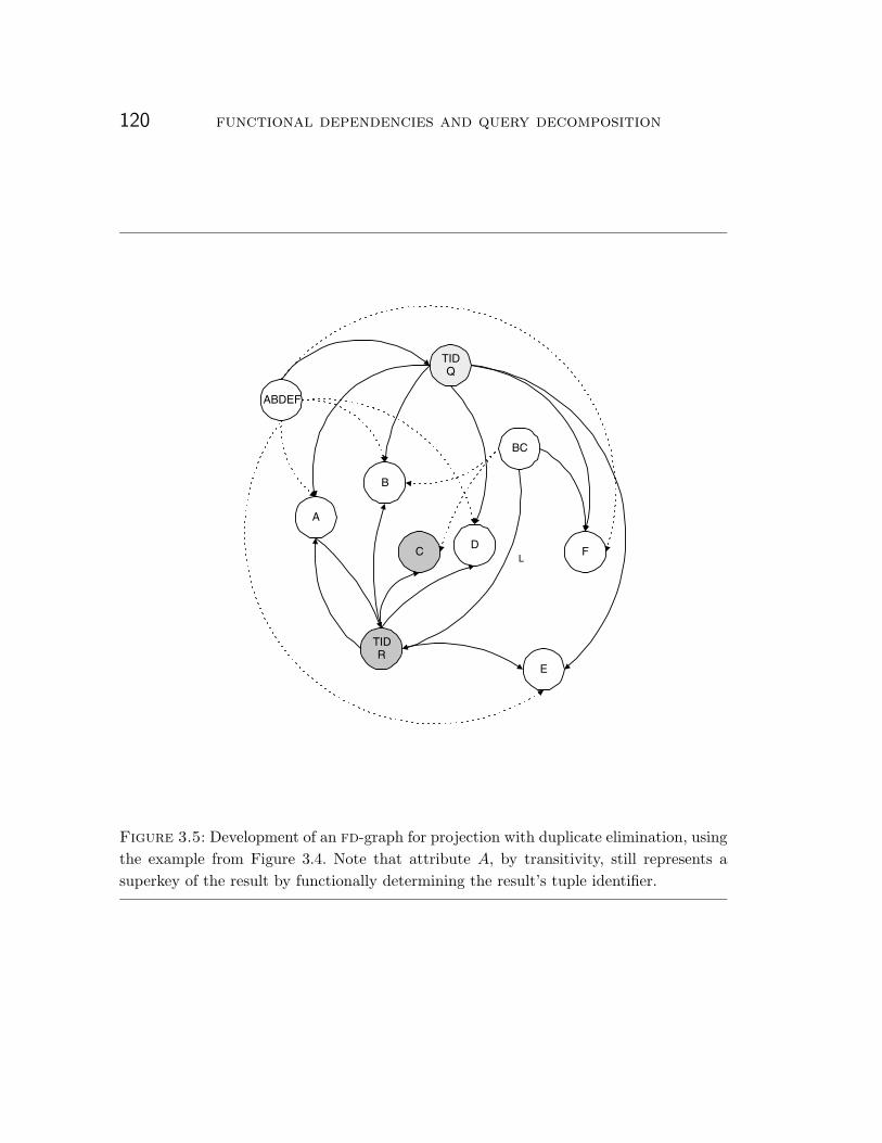
120 functional dependencies and query decomposition
CD
A
B
TIDR
BC
E
LF
TIDQ
ABDEF
Figure 3.5: Development of an fd-graph for projection with duplicate elimination, usingthe example from Figure 3.4. Note that attribute A, by transitivity, still represents asuperkey of the result by functionally determining the result’s tuple identifier.

3.4 modelling derived dependencies with fd-graphs 121
Construct vertex P ∈ V C ← {A};127
V C ← V C ∪ P ;128
– –Add the dotted edges for the new compound vertex.129
for each vi ∈ P130
EC ← EC ∪ (P, vi);131
od ;132
EF ← EF ∪ (P, vP )133
else134
EF ← EF ∪ (A, vP )135
fi136
fi ;137
return GQ138
end139
3.4.4 Cartesian product
Figure 3.6 illustrates the fd-graph formed to represent the Cartesian product of ex-tended table R with real attributes ABCDE, whose fd-graph appears in Figure 3.3, andextended table T with real attributes MNPQ and primary key MN . Note from the re-sulting fd-graph that two superkeys, namely {MNA} and {MNBC}, can be inferredfrom the fd-graph. The latter is a lax superkey because BC constitutes a unique con-straint in R. However, subsequent discovery of a null-intolerant predicate in a Where orHaving clause will trigger the conversion of lax dependencies to strict ones, and if so thenMNBC still has the possibility of forming a strict candidate key (see Section 3.4.5 be-low).
An optimization to this algorithm, though omitted in this thesis, is to recognize thatif we can guarantee that either of the inputs can have at most one tuple then constructinga combined tuple identifier vertex is unnecessary.
Procedure: Cartesian-product140
Purpose: Construct an FD-graph for Q = R× T .141
Inputs: fd-graphs GR and GT .142
Output: fd-graph GQ.143
begin144
Merge graphs GR and GT into GQ;145
– –Add a new tuple id vertex to represent a tuple in the derived result.146
Construct vertex vK ∈ V R as a tuple identifier;147
V R ← V R ∪ vK ;148
Colour[vK ] ← Gray;149
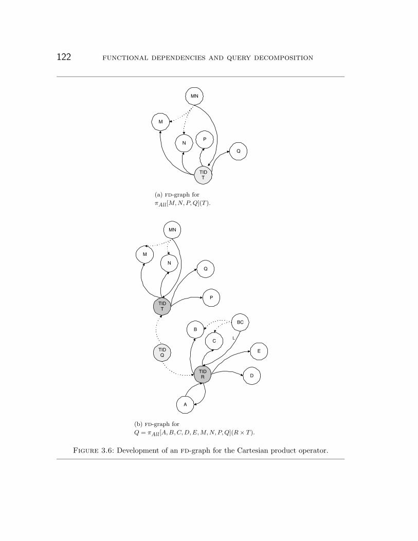
122 functional dependencies and query decomposition
NP
M
TIDT
MN
Q
(a) fd-graph for
πAll [M,N,P,Q](T ).
N
P
M
TIDT
MN
Q
C
D
A
B
TIDR
BC
E
L
TIDQ
(b) fd-graph for
Q = πAll [A,B,C,D,E,M,N, P,Q](R× T ).
Figure 3.6: Development of an fd-graph for the Cartesian product operator.

3.4 modelling derived dependencies with fd-graphs 123
vR ← v ∈ V R[GR] such that Colour[v] is Gray;150
ER ← ER ∪ (vK , vR);151
Colour[vR] ← Black;152
vT ← v ∈ V R[GT ] such that Colour[v] is Gray;153
ER ← ER ∪ (vK , vT );154
Colour[vT ] ← Black;155
return GQ156
end157
3.4.5 Restriction
The algebraic restriction operator R′ = σ[C](R) is used for both Where and Having
clauses (see Section 2.3.1.4). Restriction is one operator that can only add strict func-tional dependencies to F ; it cannot remove any existing strict dependencies.Extension. If we detect a scalar function λ(X) during the analysis of a Where clause, thenwe call the extension procedure to construct a vertex to represent λ(X) and the (strict)functional dependency X −→ λ(X) in the fd-graph. Since λ(X) is a virtual attribute inρ(R′), we colour its vertex black.
Conversion of lax dependencies. In the algorithm below we assume that each conjunct ofthe restriction predicate is false-interpreted. In this case, any Type 1 or Type 2 equalitycondition concerning an attribute v will automatically eliminate any tuples from the re-sult where v is the null value. Hence any algebraic operator higher in the expression treecan be guaranteed that v cannot be Null. Consequently we can mark v as definite in thefd-graph, and we can do so transitively for any other attribute equated to v. The follow-ing sub-procedure, set definite, appropriately marks vertices in the set V A as definite,and does so transitively using the temporary set S. The temporary vertex characteris-tic ‘Visited’ ensures that no attribute vertex is considered more than once.
Procedure: Set definite158
Purpose: Mark each vertex in the closure of equality conditions as definite.159
Inputs: fd-graph G.160
Output: Modified fd-graph G.161
begin162
S ← ∅;163
for each vi ∈ V A do164
Visited[vi] ← False;165
if Nullability[vi] is Definite then166
S ← S ∪ vi167

124 functional dependencies and query decomposition
fi168
od ;169
while S �= ∅ do170
select vertex vi from S;171
S ← S − vi;172
Visited[vi] ← True;173
D ← Mark Definite(vi);174
for each vj ∈ D do175
Nullability[vj ] ← Definite;176
if Visited[vj ] is False then177
S ← S ∪ vj178
fi179
od180
od ;181
return G182
end183
The mark definite procedure below returns a set D of related attributes that canbe treated as definite due to the existence of a strict equality constraint between eachattribute in D and the input parameter, vertex v. The test for vertex colour ensures thatwe do not attempt to mark a vertex in V A
κ representing a Null constant as definite.
Procedure: Mark definite184
Purpose: Construct a set of vertices that can be considered definite.185
Inputs: fd-graph G, vertex v.186
Output: A set D consisting of those vertices related to v that can be made definite.187
begin188
D ← ∅;189
for each vi ∈ V A such that (v, vi) ∈ EE do190
if Nullability[vi] is not Definite and Colour[vi] is not Gray then191
D ← D ∪ vi192
fi193
od ;194
return D195
end196

3.4 modelling derived dependencies with fd-graphs 125
We can convert any lax dependencies or equivalence constraints into strict ones oncewe can determine that both the left- and right-hand sides of the constraint cannot beNull. The following sub-procedure, convert dependencies, transforms lax dependen-cies or equivalence constraints between any two vertices that represent definite valuesinto strict ones. In the case of composite determinants, we check that each of the indi-vidual component vertices that constitute the determinant are marked definite.
Procedure: Convert dependencies197
Purpose: Convert lax dependencies and equivalence constraints into strict ones.198
Inputs: fd-graph G.199
Output: Modified fd-graph G.200
begin201
for each edge (vi, vj) ∈ Ef do202
– –Note that vertex vj can only exist in V A ∪ V R.203
if vi ∈ V A and Nullability[vi] is Definite then204
if vj ∈ V R then205
Ef ← Ef − (vi, vj);206
EF ← EF ∪ (vi, vj)207
else208
if vj ∈ V A and Nullability[vj ] is Definite then209
Ef ← Ef − (vi, vj);210
EF ← EF ∪ (vi, vj)211
if (vi, vj) ∈ Ee then212
Ee ← Ee − (vi, vj);213
EE ← EE ∪ (vi, vj)214
fi215
fi216
fi217
else218
if vi ∈ V C then219
if ∃ vk such that (vi, vk) ∈ EC and Nullability[vk] is not Definite then220
continue221
fi222
if vj ∈ V R then223
Ef ← Ef − (vi, vj);224
EF ← EF ∪ (vi, vj)225
else226
if vj ∈ V A and Nullability[vj ] is Definite then227
Ef ← Ef − (vi, vj);228
EF ← EF ∪ (vi, vj)229
fi230

126 functional dependencies and query decomposition
fi231
fi232
fi233
od ;234
return G235
end236
The restriction procedure assumes that the given restriction predicate is in con-junctive normal form, and immediately eliminates all disjunctive clauses. For each re-maining Type 1 or Type 2 condition, the procedure adds the necessary vertices if they donot already exist, marks the vertices as definite, and adds the appropriate (strict) depen-dency and equivalence edges. In the last two steps of the procedure, the sub-proceduresset definite and convert dependencies are called to first mark those vertices in V A
that are guaranteed to be definite through transitive strict equivalence constraints, andsecond to convert lax dependencies and equivalence constraints into strict ones if boththeir determinants and dependents cannot be Null.
Procedure: Restriction237
Purpose: Construct an FD-graph for Q = σ[C](R).238
Inputs: fd-graph G; restriction predicate C.239
Output: fd-graph GQ.240
begin241
copy G to GQ;242
separate C into conjuncts: C ′ ← P1 ∧ P2 ∧ . . . ∧ Pn;243
for each Pi ∈ C ′ do244
if Pi contains an atomic condition not of Type 1 or Type 2 then245
delete Pi from C ′246
else if Pi contains a disjunctive clause then247
delete Pi from C ′248
fi249
fi250
od251
if C ′ is simply True then return GQ fi ;252
– –C ′ now consists of entirely conjunctive components.253
vK ← v ∈ V R such that Colour[v] is Gray;254
for each conjunctive predicate Pi ∈ C ′ do255
if Pi is a Type 1 condition (v = c) then256
V A ← V A ∪ χ(c);257
if v is a function λ(X) then258
call Extension(GQ,X, v, vK);259

3.4 modelling derived dependencies with fd-graphs 127
Colour[χ(v)] ← Black260
fi ;261
– –This condition will eliminate all null values of v.262
Nullability[χ(c)] ← Definite;263
Nullability[χ(v)] ← Definite;264
Colour[χ(c)] ← Gray;265
EF ← EF ∪ (χ(v), χ(c)) ∪ (χ(c), χ(v));266
EE ← EE ∪ (χ(v), χ(c))267
else268
– –Component Pi is a Type 2 condition (v1 = v2).269
if v1 is a function λ(X) then270
call Extension(GQ,X, v1, vK);271
Colour[χ(v1)] ← Black272
fi ;273
if v2 is a function λ(X) then274
call Extension(GQ,X, v2, vK);275
Colour[χ(v2)] ← Black276
fi277
– –This condition will eliminate all null values of both v1 and v2.278
Nullability[χ(v1)] ← Definite;279
Nullability[χ(v2)] ← Definite;280
EF ← EF ∪ (χ(v1), χ(v2)) ∪ (χ(v2), χ(v1));281
EE ← EE ∪ (χ(v1), χ(v2))282
fi283
od ;284
Call SetDefinite(GQ);285
Call ConvertDependencies(GQ);286
return GQ287
end288
Handling true-interpreted predicates. In the algorithm above, we presented only the pseudo-code for analyzing false-interpreted predicates. In cases where the restriction conditioncontains one or more conjunctive true-interpreted Type 1 or Type 2 conditions, thepseudo-code would be nearly identical but for a modification to generate lax dependen-cies and equivalence constraints instead of strict ones. Essentially the main loop fromlines 255 through 284 would be repeated, with:
• the lines which set each vertex’s nullability characteristic to ‘definite’ removed(lines 263, 264, 279, and 280); and

128 functional dependencies and query decomposition
• lines which add strict functional dependencies (lines 266 and 281) and strict equiv-alence constraints (lines 267 and 282) changed to add lax functional dependenciesand equivalence constraints, respectively.
The existence of a true-interpreted predicate will not alter the validity of any strict de-pendency or equivalence constraint previously discovered, nor does it affect the logic ofthe procedures Set Definite or Convert Dependencies.
3.4.6 Intersection
The fd-graph GQ representing the intersection of extended tables S and T is constructedby performing a union of the fd-graphs for S and T and adding equivalence and strictdependency edges between the corresponding white vertices of their inputs, which corre-spond to the select list items of each query specification (see Figure 3.7). We assume thatthe merging of the two fd-graphs results in a graph where all attributes are uniquelynamed. We arbitrarily denote attributes from S to constitute the result of the intersec-tion, and colour black all white attributes from T to model their inclusion as virtual at-tributes in Q.
To represent a tuple in the instance I(Q), we arbitrarily choose the tuple identifierof S, and add strict dependency edges between the two tuple identifier vertices of theinputs. The tuple identifier of T is coloured black23. With this construction, if a completesimple or composite candidate superkey is present in either input, then that key becomesa superkey of the result (as per Corollary 1 on page 80).
Finally, we mark as pseudo-definite any vertex representing a real attribute of S if itor its corresponding attribute in T is pseudo-definite, since there exists a strict equiva-lence constraint between each attribute pair and by the semantics of intersection the cor-responding values of each attribute pair are identical. Moreover, the procedure Set Def-inite may now be able to exploit these strict equivalence constraints to mark either ofthese corresponding vertices as definite. Set Definite can also exploit the existence ofother strict equivalence constraints in either input to mark some subset of the attributesin sch(Q) as definite. Subsequently, we may be able to convert lax functional dependen-cies and lax equivalence constraints to strict ones in a manner identical to that for therestriction operator.
23 Recall the invariant that there must be one, and only one, tuple identifier vertex in V R
coloured gray in an fd-graph.

3.4 modelling derived dependencies with fd-graphs 129
C
DA
B E
BCE
F
TIDS
(a) fd-graph for πAll [A,B, F ](S).
Y
W
X
XY
Z
TIDT
(b) fd-graph for
πAll [X,W,Z](T ).
Y
W
X
XY
Z
TIDT
C
D
A
B
E
BCE
F
TIDS
(c) fd-graph for Q =
πAll [A,B, F ](S) ∩All πAll [X,W,Z](T ).
Figure 3.7: Development of an fd-graph for the Intersection operator. Note that thevertex representing A denotes a superkey of the result.

130 functional dependencies and query decomposition
Procedure: Intersection289
Purpose: Construct an FD-graph for Q = S ∩All T .290
Inputs: fd-graphs GS and GT .291
Output: fd-graph GQ.292
begin293
Merge graphs GS and GT into GQ;294
– –Choose the tuple id vertex of S to represent a tuple in I(Q).295
vS ← v ∈ V R[GS ] such that Colour[v] is Gray;296
vT ← v ∈ V R[GT ] such that Colour[v] is Gray;297
EF ← EF ∪ (vS , vT ) ∪ (vT , vS);298
Colour[vT ] ← Black;299
– –Establish equivalences between the white vertices in GT and GS.300
for each white vertex vk ∈ V A[GT ] do301
– –Let vi denote the corresponding white attribute from GT in GQ.302
– –Let vj denote the union-compatible white attribute from GS in GQ.303
EF [GQ]← EF [GQ] ∪ (vi, vj) ∪ (vj , vi);304
EE [GQ]← EE [GQ] ∪ (vi, vj);305
Colour[vi] ← Black;306
if Nullability[vi] is Pseudo-definite and Nullability[vj ] is Nullable then307
Nullability[vj ] ← Pseudo-definite308
fi ;309
if Nullability[vj ] is Pseudo-definite and Nullability[vi] is Nullable then310
Nullability[vi] ← Pseudo-definite311
fi312
od ;313
Call SetDefinite(GQ);314
Call ConvertDependencies(GQ);315
return GQ316
end317
3.4.7 Grouping and Aggregation
As described in Section 2.3 we model sql’s group-by operator with two algebraic opera-tors. The partition operator, denoted G, produces a grouped table as its result with onetuple per distinct set of group-by attributes. Each set of values required to compute anyaggregate function is modelled as a set-valued attribute. The grouped table projection op-erator, denoted P, projects a grouped table over a Select list composed of group-by at-tributes and aggregate function applications. Projection of a grouped table differs froman ‘ordinary’ projection in that it must deal not only with atomic attributes (those in

3.4 modelling derived dependencies with fd-graphs 131
the Group by list) but also the set-valued attributes used to compute the aggregate func-tions.
3.4.7.1 Partition
The algorithm begins with creating a new tuple identifier vK to represent each tuplein the partition; the tuple identifier of the original input vI , now a virtual attribute inρ(Q), is coloured black. Subsequently, the Extension procedure is called to create addi-tional vertices for any scalar functions λ(X) present in the group-by list. These new at-tributes are coloured white since they are real attributes in the extended table Q that re-sults from the partition. Thereafter the algorithm colours black any vertex that does notrepresent a real attribute—that is, a group-by attribute or a set-valued attribute requiredfor one or more aggregate functions—to denote its assignment to ρ(Q). Finally, we createa superkey K consisting of the entire group-by list (if one exists) which forms the deter-minant of the set of strict functional dependencies for each of the set-valued attributes. Ifthere already exists a superkey vertex X in the input—for example, the Group by clausecontains the primary key(s) of the input base table(s)—then it follows that X ⊆ K andconsequently we trivially have X −→ K and K −→ X. These other keys will then in-fer K, and consequently the fd-graph reflects all of the valid superkeys.
In Claim 22 (see page 83) we noted that a special case of partition is when the set AG
is empty, corresponding to a missing Group by clause in an aggregate ansi sql query. Inthis case, the result must consist of a single tuple containing one or more set-valued at-tributes containing the values required by each aggregation function f ∈ F . In this case,we model the key of the result by using a constant attribute. To ensure that we do not in-fer erroneous transitive dependencies or equivalence constraints from this constant, weassume that the value of the constant is definite and unique across the entire databaseinstance (and hence unequal to any other constant discovered during dependency analy-sis). We assume the existence of a generating function ℵ() that produces such a uniquevalue when required.
Procedure: Partition318
Purpose: Construct an FD-graph for Q = G[AG, AA](R).319
Inputs: fd-graph G; n grouping attributes AG;320
m set-valued attributes AA.321
Output: fd-graph GQ.322
begin323
copy G to GQ;324
– –Add a new tuple id vertex to represent a tuple in I(Q).325
vI ← v ∈ V R such that Colour[v] is Gray;326
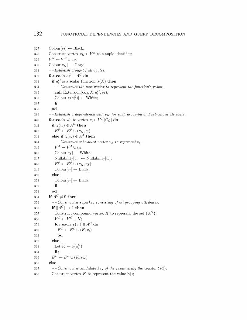
132 functional dependencies and query decomposition
Colour[vI ] ← Black;327
Construct vertex vK ∈ V R as a tuple identifier;328
V R ← V R ∪ vK ;329
Colour[vK ] ← Gray;330
– –Establish group-by attributes.331
for each aGi ∈ AG do332
if aGi is a scalar function λ(X) then333
– –Construct the new vertex to represent the function’s result.334
call Extension(GQ,X, aGi , vI);335
Colour[χ(aGi )] ← White;336
fi337
od ;338
– –Establish a dependency with vK for each group-by and set-valued attribute.339
for each white vertex vi ∈ V A[GQ] do340
if χ(vi) ∈ AG then341
EF ← EF ∪ (vK , vi)342
else if χ(vi) ∈ AA then343
– –Construct set-valued vertex vS to represent vi.344
V A ← V A ∪ vS ;345
Colour[vS ] ← White;346
Nullability[vS ] ← Nullability[vi];347
EF ← EF ∪ (vK , vS);348
Colour[vi] ← Black349
else350
Colour[vi] ← Black351
fi352
od ;353
if AG �= ∅ then354
– –Construct a superkey consisting of all grouping attributes.355
if ‖AG‖ > 1 then356
Construct compound vertex K to represent the set {AG};357
V C ← V C ∪K;358
for each χ(vi) ∈ AG do359
EC ← EC ∪ (K, vi)360
od361
else362
Let K ← χ(aG1 )363
fi ;364
EF ← EF ∪ (K, vK)365
else366
– –Construct a candidate key of the result using the constant ℵ().367
Construct vertex K to represent the value ℵ();368

3.4 modelling derived dependencies with fd-graphs 133
V A ← V A ∪K;369
Colour[K] ← Gray;370
Nullability[K] ← Definite;371
EF ← EF ∪ (K, vK)372
fi ;373
return GQ374
end375
3.4.7.2 Grouped table projection
The projection of a grouped table, denoted P, projects a grouped table over the set ofgrouping columns and represents the computation of any aggregate functions over oneor more set-valued attributes. The Grouped Table Projection algorithm below com-putes the derived dependencies that hold in the result of Q = P[AG, F [AA]](R). As de-scribed earlier, the number of tuples in Q is identical to the number of tuples in the ex-tended grouped table R, hence no tuple identifier modifications are necessary. Set-valuedattributes do not themselves appear in the projection; only grouping columns or the re-sult of an aggregate function fi can appear as real attributes in the result, and hencethese input attributes are coloured black. Each aggregate function in the result is cre-ated by extending Q through a call to the Extension procedure; the resulting vertex iscoloured white to represent its membership in α(Q).
Procedure: Grouped Table Projection376
Purpose: Construct an FD-graph for Q = P[AG, F [AA]](R).377
Inputs: fd-graph G; n grouping attributes AG;378
m set-valued attributes AA, k aggregate functions.379
Output: fd-graph GQ.380
begin381
copy G to GQ;382
vK ← v ∈ V R such that Colour[v] is Gray;383
– –Colour black all set-valued attributes that cannot exist in the projection.384
for each white vertex vi ∈ V A do385
if χ(vi) �∈ AG then386
– – vi is a set-valued aggregation attribute, which cannot be in the result.387
Colour[vi] ← Black388
fi389
od ;390
for each fi ∈ F | 1 ≤ i ≤ k do391
– –Construct a vertex Y to represent fi(AAj ) and392

134 functional dependencies and query decomposition
– –make its set-valued input parameters its determinant.393
call Extension(GQ, AAj , Y, vK);394
Colour[Y ] ← White;395
if fi = ‘Count’ or ‘Count Distinct’ then396
Nullability[Y ] ← Definite397
else398
Nullability[Y ] ← Nullable399
fi400
od ;401
return GQ402
end403
3.4.8 Left outer join
As mentioned previously in Section 3.3.1.7, for left outer joins we require a mechanismto group the attributes from the null-supplying side of an outer join so that once a null-intolerant Where clause predicate is discovered, all of the lax dependencies and lax equiv-alence constraints amongst the pseudo-definite attributes in the group—which form anull constraint—can be converted to strict dependencies and equivalence constraints. Togroup null-supplying attributes together, we utilize a hypervertex in V J with mixed edgesin EJ to each of its component vertices. In the case of nested outer joins, an edge in EJ
may connect two vertices in V J (see Figure 3.8). These edges form a tree of vertices inV J , which represent each level of nesting in much the same way Bhargava, Goel, and Iyer[34] use levels of binding to determine the candidate keys of the results of outer joins24.
Example 22
Consider the fd-graph pictured in Figure 3.9. The fd-graph illustrates the functionaldependencies that hold in the result of the expression
Q = Rα(πAll [W,X,A,B](Tp−→ S)) (3.4)
24 For full outer joins each side of the join will be represented by a separate instance of a vertexin V J ; see Section 3.4.9.

3.4 modelling derived dependencies with fd-graphs 135
FOJ4
T W
S
R
FOJ3
LOJ1
LOJ2
Figure 3.8: Summarized fd-graph for a nested outer join modelling the expression Q =R
p1−→ (Sp2−→ (T
p3←→W )). Each vertex that represents a null-supplying side groups null-supplying attributes together. Furthermore, there exists a directed edge in EJ from eachnested null-supplying vertex to a vertex representing its ‘parent’ table expression.
over extended tables T and S with real attributesWXY Z and ABCDE respectively andwhere predicate p consists of the conjunctive condition T.X = S.B ∧ T.Z = S.A, whichcorresponds to the sql statement
Select W, X, A, B
From Rα(T) Left Outer Join Rα(S) On (T.X = S.B and T.Z = S.A)
where XY is the primary key of T and A is the primary key of S. Note the existence ofthe lax functional dependency A −→ Z and its corresponding lax equivalence constraintA ) Z, due to the fact that S is the null-supplying table. Note also that A −→ BCDE re-mains reflected as four strict dependencies since A is a primary key and hence cannot beNull. The strict dependency B −→ D has been transformed from a lax dependency inthe input; the conjunctive predicate T.X = S.B in the On condition ensures that the gen-eration of an all-Null row cannot violate B −→ D even though B is nullable in extendedtable S.

136 functional dependencies and query decomposition
C
D
TIDS
B
E
LOJS
W
Y
TIDT
Z
X
L
L
XY
TIDQ
A
ZX
L
L
L
L
Figure 3.9: Resulting fd-graph for the left outer join in Example 22. Note the fourdifferent types of edges: solid edges denote functional dependencies, dotted edges linkcompound nodes to their components, dashed edges represent equivalence constraints,and mixed edges group attributes from a null-supplying side of an outer join. Note thatthe lax dependency B &−→ D, which stemmed from the nullable determinant B, has beenconverted to a strict dependency due to the null-intolerant predicate in the outer join’sOn condition.

3.4 modelling derived dependencies with fd-graphs 137
3.4.8.1 Algorithm
The algorithm below accepts three inputs: the two fd-graphs corresponding to the inputs(preserved table S, null-supplying table T ) of the left outer join, and the outer join’s Oncondition p. The algorithm’s logic can be divided into five distinct parts:
1. Graph merging and initialization (lines 410 to 430): the two input graphs are mergedinto a single graph GQ that represents the dependencies and equivalences that holdin the result. A new tuple identifier vertex vK is created to represent a derived tu-ple in the outer join’s result, and a null-supplying vertex J is created to link theattributes on the null-supplying side of the left outer join. The algorithm also as-sumes that attributes are appropriately renamed to prevent logic errors due to du-plicate names, and to simplify the exposition we assume that the On condition doesnot contain any scalar functions, although we could easily extend the algorithm todo so. The algorithm for right outer join is symmetric with the one for left, sim-ply by interchanging the two inputs.
2. Dependency and constraint analysis for the null-supplying table (lines 431 to 472):strict dependencies that hold in T are analyzed to determine if they can hold inI(Q), or if they must be ‘downgraded’ to a lax dependency because their determi-nant can be wholly Null, as per Lemma 7. As mentioned above, the algorithm re-lies on a function η, which is assumed to exist, to determine whether or not the leftouter join’s On condition can be satisfied if a given attribute can be Null. Lax de-pendencies that hold in T can also be converted to strict dependencies if the con-ditions specified in Lemma 8 hold. Moreover, lax equivalence constraints e : X ) Y
will continue to hold in Q. However, if the possibility of null values for X and Y
are eliminated but for the all-Null row—that is, both η(p,X) and η(p, Y ) returntrue—then e can be ‘upgraded’ to a strict equivalence constraint.
3. Generation of lax dependencies implied by the On condition (lines 473 to 516): fol-lowing the analysis outlined in Section 3.2.9.2, the algorithm generates a valid sub-set of the lax and strict dependencies implied by null-intolerant conjunctive equal-ity predicates in the On condition. The logic within this section is quite similarto that outlined in the Restriction algorithm. A strict dependency will only re-sult from a Type 2 condition involving two attributes from the null-supplying table;otherwise all of the generated dependencies constructed in this portion of the algo-rithm are lax dependencies.
4. Construction of strict dependencies implied by the On condition (lines 517 to 533):following the analysis outlined in Section 3.2.9.2, the algorithm generates the strict

138 functional dependencies and query decomposition
dependencies g : αS(p) −→ z between the set of preserved attributes referenced inp and each z ∈ Z, the set of null-supplying attributes included in null-intolerantconjunctive equality predicates in the On condition (see Theorem 3). The dependentset Z is constructed as a side-effect of the On condition analysis done in the previousstep.
5. Marking attributes nullable (lines 534 to 541): finally, all null-supplying attributesmust be marked as either nullable or pseudo-definite to correspond to the possiblegeneration of an all-Null row in the result.
We have simplified the algorithm below to ignore the existence of (1) is null pred-icates, (2) any other null-tolerant condition, or (3) scalar functions λ(X) in p. However,the algorithm can be easily extended to include such support, or to derive additional strictor lax dependencies depending upon the sophistication of the analysis on the On condi-tion predicate p.
Procedure: Left Outer Join404
Purpose: Construct an FD-graph for Q = Sp−→ T .405
Inputs: fd-graphs for GS , GT , predicate p.406
Output: fd-graph GQ.407
408
begin409
Merge graphs GS and GT into GQ;410
– –Add a new tuple id vertex to represent a tuple in the derived result.411
Construct vertex vK ∈ V R as a tuple identifier;412
V R ← V R ∪ vK ;413
Colour[vK ] ← Gray;414
vS ← v ∈ V R[GS ] such that Colour[v] is Gray;415
ER ← ER ∪ (vK , vS)416
Colour[vS ] ← Black;417
vT ← v ∈ V R[GT ] such that Colour[v] is Gray;418
ER ← ER ∪ (vK , vT )419
Colour[vT ] ← Black;420
– –Construct an outer join vertex J to represent null-supplying attributes in GT .421
V J [GQ]← V J [GQ] ∪ J ;422
for each vi ∈ V A[GT ] do423
if � ∃(vj , vi) ∈ EJ [GT ] for any vj ∈ V J [GT ] then424
EJ ← EJ ∪ (J, vi)425
fi426
od ;427
for each vj ∈ V J [GT ] such that � ∃ vk ∈ V J | (vj , vk) ∈ EJ do428
EJ ← EJ ∪ (vj , J)429

3.4 modelling derived dependencies with fd-graphs 139
od ;430
– –Determine those equivalences and dependencies from T that still hold in Q.431
for each strict dependency edge (vi, vj) ∈ EF do432
if vj �∈ V A[GT ] ∪ V R[GT ] then continue fi ;433
if vi ∈ V R[GT ] then continue fi ;434
if vi ∈ V A[GT ] then435
if η(p, χ(vi)) is False and (vi, vj) �∈ EE then436
EF ← EF − (vi, vj);437
Ef ← Ef ∪ (vi, vj)438
fi439
else if vi ∈ V C [GT ] then440
– –For a compound determinant, ensure it has at least one definite attribute.441
if � ∃ vk such that (vi, vk) ∈ EC and η(p, χ(vk)) is True then442
EF ← EF − (vi, vj);443
Ef ← Ef ∪ (vi, vj)444
fi445
fi446
od ;447
for each lax dependency edge (vi, vj) ∈ Ef do448
if vj �∈ V A[GT ] ∪ V R[GT ] then continue fi ;449
if vi ∈ V A[GT ] then450
if η(p, χ(vi)) is True and (vj ∈ V R or η(p, χ(vj)) is True) then451
EF ← EF ∪ (vi, vj);452
Ef ← Ef − (vi, vj);453
fi454
else if vi ∈ V C [GT ] then455
– –For a compound determinant, it must have all definite attributes.456
if ∃ vk such that (vi, vk) ∈ EC and η(p, χ(vk)) is False then457
continue458
fi459
if vj ∈ V R or η(p, χ(vj)) is True then460
EF ← EF ∪ (vi, vj);461
Ef ← Ef − (vi, vj)462
fi463
fi464
od ;465
for each lax equivalence edge (vi, vj) ∈ Ee do466
if {vi ∪ vj} �⊆ V A[GT ] then continue fi ;467
if η(p, χ(vi)) is True and η(p, χ(vj)) is True then468
EE ← EE ∪ (vi, vj);469
Ee ← Ee − (vi, vj)470
fi471
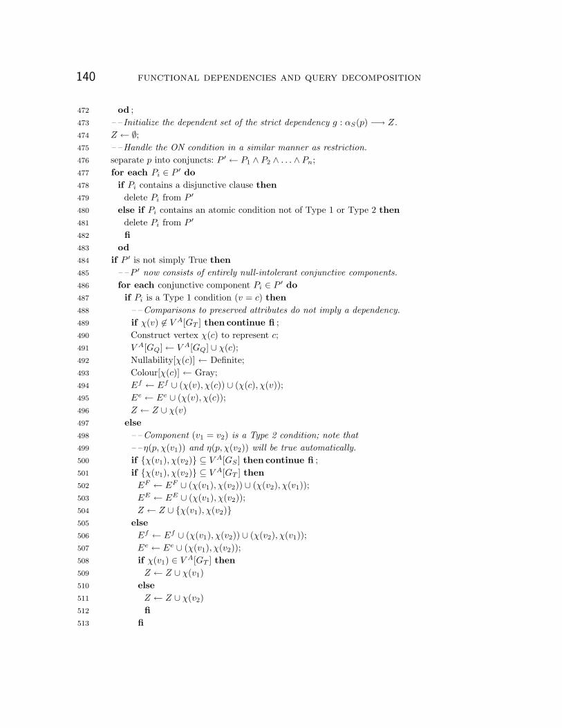
140 functional dependencies and query decomposition
od ;472
– – Initialize the dependent set of the strict dependency g : αS(p) −→ Z.473
Z ← ∅;474
– –Handle the ON condition in a similar manner as restriction.475
separate p into conjuncts: P ′ ← P1 ∧ P2 ∧ . . . ∧ Pn;476
for each Pi ∈ P ′ do477
if Pi contains a disjunctive clause then478
delete Pi from P ′479
else if Pi contains an atomic condition not of Type 1 or Type 2 then480
delete Pi from P ′481
fi482
od483
if P ′ is not simply True then484
– –P ′ now consists of entirely null-intolerant conjunctive components.485
for each conjunctive component Pi ∈ P ′ do486
if Pi is a Type 1 condition (v = c) then487
– –Comparisons to preserved attributes do not imply a dependency.488
if χ(v) �∈ V A[GT ] then continue fi ;489
Construct vertex χ(c) to represent c;490
V A[GQ]← V A[GQ] ∪ χ(c);491
Nullability[χ(c)] ← Definite;492
Colour[χ(c)] ← Gray;493
Ef ← Ef ∪ (χ(v), χ(c)) ∪ (χ(c), χ(v));494
Ee ← Ee ∪ (χ(v), χ(c));495
Z ← Z ∪ χ(v)496
else497
– –Component (v1 = v2) is a Type 2 condition; note that498
– – η(p, χ(v1)) and η(p, χ(v2)) will be true automatically.499
if {χ(v1), χ(v2)} ⊆ V A[GS ] then continue fi ;500
if {χ(v1), χ(v2)} ⊆ V A[GT ] then501
EF ← EF ∪ (χ(v1), χ(v2)) ∪ (χ(v2), χ(v1));502
EE ← EE ∪ (χ(v1), χ(v2));503
Z ← Z ∪ {χ(v1), χ(v2)}504
else505
Ef ← Ef ∪ (χ(v1), χ(v2)) ∪ (χ(v2), χ(v1));506
Ee ← Ee ∪ (χ(v1), χ(v2));507
if χ(v1) ∈ V A[GT ] then508
Z ← Z ∪ χ(v1)509
else510
Z ← Z ∪ χ(v2)511
fi512
fi513

3.4 modelling derived dependencies with fd-graphs 141
fi514
od515
fi516
– –Construct the strict dependency of preserved attributes to null-supplying ones.517
if ‖αS(p)‖ > 0 then518
if ‖αS(p)‖ > 1 then519
– –Create a compound determinant in V C for the dependency g.520
Construct vertex W ∈ V C to represent αS(p);521
V C ← V C ∪W ;522
– –Add the dotted edges for the new compound vertex.523
for each vi ∈W524
EC ← EC ∪ (W, vi);525
od ;526
else527
Let χ(W ) denote the single preserved vertex in αS(p);528
fi529
for each vk ∈ Z do530
EF ← EF ∪ (W, vk)531
od532
fi ;533
– –Finally, set the nullability characteristic of each attribute from the null-supplying side.534
for each vi ∈ V A[GT ] do535
if η(p, χ(vi)) is True then536
Nullability[vi[GQ]] ← Pseudo-definite537
fi538
od539
return GQ540
end541
3.4.9 Full outer join
Because full outer join only differs slightly in its semantics from left or right outer join, weomit the presentation of a detailed algorithm to construct an fd-graph representing thedependencies and equivalences that hold in the result of a full outer join. We claim thatwe can modify the left outer join algorithm in a straightforward manner, followingTheorem 4, to model the correct semantics for full outer join.

142 functional dependencies and query decomposition
3.4.10 Algorithm modifications to support outer joins
Galindo-Legaria and Rosenthal [97, 98] and Bhargava and Iyer [33] both describe queryrewrite optimizations to convert outer joins to inner joins, or full outer joins to left (orright) outer joins, via the analysis and exploitation of strong predicates specified in thequery. Such rewrite transformations are beyond the scope of this thesis. However, we dorecognize that the presence of null-intolerant predicates in a Where or Having clause con-verts lax dependencies and equivalence constraints into strict ones. This result followsfrom the following algebraic identities [98, pp. 50]:
σ[C1](RC2−→ S) ≡ σ[C1 ∧ C2](R× S) if C1 rejects null values
on α(S)(3.5)
σ[C1](RC2←→ S) ≡ σ[C1](R
C2←− S) if C1 rejects null valueson α(S)
(3.6)
Consequently we modify the restriction algorithm to determine when lax dependen-cies can be transformed to strict ones by recognizing the existence of any null constraints.To do so simply involves modifying the mark definite procedure to augment the set ofvertices in an fd-graph that can be treated as definite to include those marked as pseudo-definite. If the input parameter to mark definite() is part of the null-supplying side ofa left- or full outer join, then all other pseudo-definite attributes—those that are guaran-teed not to be Null except for the generated all-Null row—can also be marked as def-inite attributes by the calling set definite procedure. Attributes that are marked aspseudo-definite as the result of a nested outer join can also be treated as definite, sincethe restriction condition will eliminate the all-Null row for the entire null-supplying ta-ble expression. Subsequently, the convert dependencies procedure can convert lax de-pendencies and equivalence edges based on these attributes to strict ones.
Procedure: Mark definite542
Purpose: Construct a set of vertices that can be considered definite.543
Note: Replaces previous version of pseudo-code with lines numbered 184 through 196.544
Inputs: fd-graph G, vertex v.545
Output: A set D consisting of those vertices related to v that can be made definite.546
begin547
D ← ∅;548
for each vi ∈ V A such that (v, vi) ∈ EE do549
if Nullability[vi] is not Definite and Colour[vi] is not Gray then550
D ← D ∪ vi551
fi552
od ;553
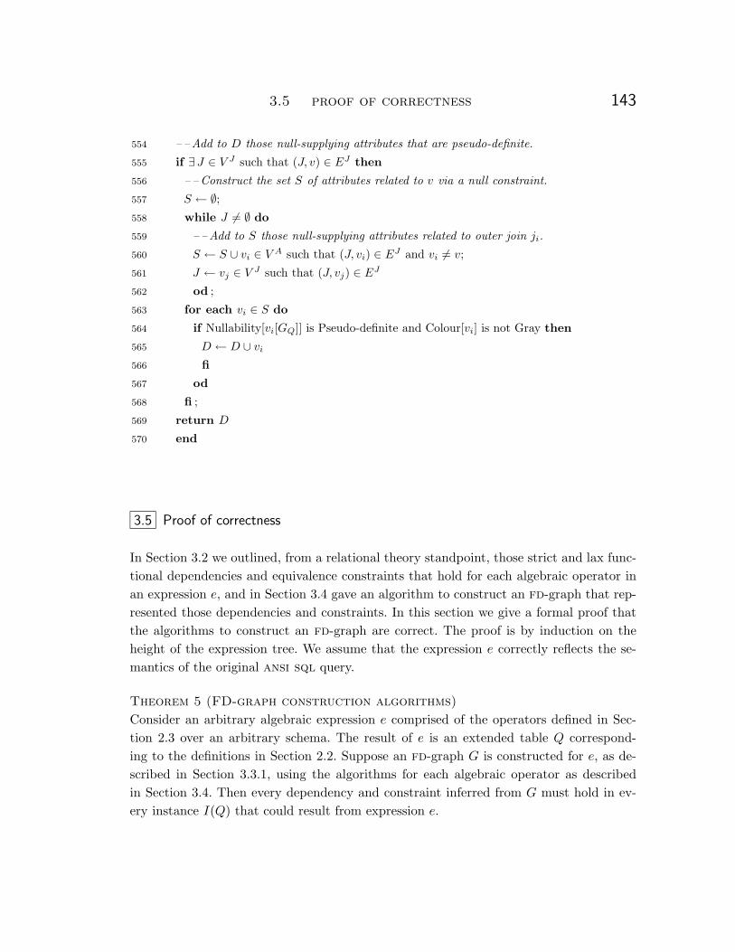
3.5 proof of correctness 143
– –Add to D those null-supplying attributes that are pseudo-definite.554
if ∃J ∈ V J such that (J, v) ∈ EJ then555
– –Construct the set S of attributes related to v via a null constraint.556
S ← ∅;557
while J �= ∅ do558
– –Add to S those null-supplying attributes related to outer join ji.559
S ← S ∪ vi ∈ V A such that (J, vi) ∈ EJ and vi �= v;560
J ← vj ∈ V J such that (J, vj) ∈ EJ561
od ;562
for each vi ∈ S do563
if Nullability[vi[GQ]] is Pseudo-definite and Colour[vi] is not Gray then564
D ← D ∪ vi565
fi566
od567
fi ;568
return D569
end570
3.5 Proof of correctness
In Section 3.2 we outlined, from a relational theory standpoint, those strict and lax func-tional dependencies and equivalence constraints that hold for each algebraic operator inan expression e, and in Section 3.4 gave an algorithm to construct an fd-graph that rep-resented those dependencies and constraints. In this section we give a formal proof thatthe algorithms to construct an fd-graph are correct. The proof is by induction on theheight of the expression tree. We assume that the expression e correctly reflects the se-mantics of the original ansi sql query.
Theorem 5 (FD-graph construction algorithms)
Consider an arbitrary algebraic expression e comprised of the operators defined in Sec-tion 2.3 over an arbitrary schema. The result of e is an extended table Q correspond-ing to the definitions in Section 2.2. Suppose an fd-graph G is constructed for e, as de-scribed in Section 3.3.1, using the algorithms for each algebraic operator as describedin Section 3.4. Then every dependency and constraint inferred from G must hold in ev-ery instance I(Q) that could result from expression e.

144 functional dependencies and query decomposition
Table Scan
Nested-loopexists join
Part
Supply
on P.PartID = S.PartID
Project
Sort by P.PartID
Index Scan Index Scan
Vendor
Nested-loopinner join
P.PartID
on V.VendorID = S.VendorID
S.VendorID
Restrict Restrict
on S.Rating and S.LagtimeOn V.Address
X
XY
Y
W
Z
V
F Γ
1 2
3
4Figure 3.10: fd-graph proof overview for strict functional dependencies.
3.5.1 Proof overview
As discussed earlier, our interest in maintaining fd-graphs is to exploit strict functionaldependencies, strict superkeys, and strict equivalences in optimizing algebraic expressiontrees. However, since we derive strict dependencies and equivalences from their lax equiv-alents when conditions warrant, we must also show that we correctly maintain fd-graphconstructs pertaining to lax functional dependencies, lax equivalence constraints, and nullconstraints. Figure 3.10 illustrates an overview of the proof procedure as applied to strictfunctional dependencies only. Previously, in Section 3.2, we described a subset of the setof strict functional dependencies F that are implied by the semantics of each algebraic op-erator and hold in its result Q (denoted as transformation (1) in Figure 3.10). The set ofstrict functional dependencies Γ represented in an fd-graph—transformation (2) in Fig-ure 3.10—is provided by an extended definition of the mapping function χ.

3.5 proof of correctness 145
Definition 46 (Dependencies and equivalence constraints in an fd-graph)
In Section 3.4 we introduced the function χ() that served to map attribute names tosimple vertices and vice-versa in an fd-graph. We now redefine χ() to be a polymorphicfunction that provides the following correspondences:
• for each vertex v ∈ V A the function χ(v) returns the unique name of attribute v(and vice-versa).
• for each vertex v ∈ V R the function χ(v) returns the unique name given to thetuple identifier ι(R) of its corresponding base or derived table R (and vice-versa).
• χ({v1, v2, . . . , vn}) = {χ(v1), χ(v2), . . . , χ(vn)}.
Furthermore, we extend χ to provide mappings from other features of an fd-graph tocharacteristics of its corresponding extended table as follows:
• χ(v ∈ V C) = {χ(b) | (v, b) ∈ EC}.
• χ(EC) = {χ(v) −→ χ(y) | v ∈ V C ∧ (v, y) ∈ EC}.
• χ(EF ) = {χ(x) −→ χ(y) | (x, y) ∈ EF }.
• χ(ER) = {χ(x) −→ χ(y) | (x, y) ∈ ER} ∪ {Y −→ χ(x) | x ∈ ER ∧ Y = {χ(y) |(x, y) ∈ ER} }.
• χ(Ef ) = {χ(x) &−→ χ(y) | (x, y) ∈ Ef}.
• χ(EE) = {χ(x) = χ(y) | (x, y) ∈ EE}.
• χ(Ee) = {χ(x) ) χ(y) | (x, y) ∈ Ee}.
These additional mappings define the set of functional dependencies and equivalence con-straints represented by an fd-graph. Note that χ cannot be used to map functional de-pendencies or equivalence constraints that may exist in an extended table to componentsin its corresponding fd-graph since not all such dependencies and constraints may be cap-tured by the fd-graph.
We denote the complete set of strict dependencies modelled by an fd-graph with Γ,which is equivalent to χ(EC)∪χ(EF )∪χ(ER). The combined set of strict and lax depen-dencies γ modelled by an fd-graph is equivalent to Γ∪χ(Ef ), since by inference rule fd5(weakening) any strict functional dependency is a lax dependency. Similarly, the com-plete set of strict equivalence constraints modelled by an fd-graph, which we denote as

146 functional dependencies and query decomposition
Type Mapping
strict functional dependencies Γ = χ(EC) ∪ χ(EF ) ∪ χ(ER)
lax functional dependencies γ = Γ ∪ χ(Ef )
strict equivalence constraints Ξ = χ(EE)
lax equivalence constraints ξ = Ξ ∪ χ(Ee)
Table 3.2: Summary of constraint mappings in an fd-graph
Ξ, and the complete combined set of strict and lax equivalence constraints, which we de-note as ξ, are equivalent to χ(EE) and χ(Ee)∪χ(EE) respectively. These definitions aresummarized in Table 3.2.
What remains to be proved is that the transformation (3) is well-defined and resultsin the subset relationship Γ ⊆ F represented by (4) in Figure 3.10. Proof of (3) showsthat each algorithm in Section 3.4 manipulates its input fd-graph(s) correctly, resultingin an fd-graph that correctly mirrors the schema of the extended table that constitutesthe result Q of the algebraic expression e:
(1) v ∈ V A ∧ colour[v] is white ⇐⇒ χ(v) ∈ α(Q)
(2) v ∈ V R ∧ colour[v] is gray ⇐⇒ χ(v) ∈ ι(Q)
(3) v ∈ V A ∧ colour[v] is gray ⇐⇒ χ(v) ∈ κ(Q)
(4) v ∈ V A ∪ V R ∧ colour[v] is black ⇐⇒ χ(v) ∈ ρ(Q)
(5) v ∈ V A ∧ Nullability[v] is definite =⇒ χ(v) is a definite attribute in I(Q).Proof of (4) requires that we show for each strict dependency f ∈ Γ that its counter-
part in F holds; that is, Γ ⊆ F . Similarly, we must also prove that any null constraints,strict equivalence constraints (the set Ξ), lax functional dependencies (the set γ), andlax equivalence constraints (the set ξ) derived from an fd-graph are guaranteed to holdin our extended relational model. More formally, for any sets of attributes X and Y andatomic attributes w and z such that XY zw ⊆ sch(Q):
(1) X −→ Y ∈ Γ =⇒ χ(X) −→ χ(Y ) ∈ FQ
(2) X &−→ Y ∈ γ =⇒ χ(X) &−→ χ(Y ) ∈ FQ
(3) wω= z ∈ Ξ =⇒ χ(w) ω= χ(z) ∈ EQ
(4) w ) z ∈ ξ =⇒ χ(w) ) χ(z) ∈ EQ(5) isNullConstraint(w, z) =⇒ w + z holds in I(Q).
where isNullConstraint is a procedure defined in Section 3.5.1.2 below that deter-mines whether or not a null constraint exists between two attributes in sch(Q).

3.5 proof of correctness 147
3.5.1.1 Assumptions for complexity analysis
Along with the proof of correctness for each algorithm, we will also present a brief worst-case complexity analysis of each. For this analysis we assume that an extended fd-graphis implemented as follows. Each set of vertices in V is represented using a hash table. Thehash key of attribute vertices is their unique name, which corresponds to our vertex map-ping function χ. The hash tables for the other vertex sets utilize the polymorphic ver-sion of χ. We further assume that fd-graph edges are represented using adjacency lists.Directed edges are linked as usual from their source vertex; we assume that undirectededges between attribute vertices vi and vj in V A which represent equivalence edges ap-pear in the adjacency lists for both vi and vj , thereby doubling their maintenance cost.With this construction, we assume that we can perform:
• constant-time (O(1)) vertex lookup and insertion, and
• constant-time edge lookup, insertion, and deletion.
We believe these assumptions are defensible with the availability of sophisticated, low-costhash-based data structures. For example, consider the dynamic hash tables recently pro-posed by Dietzfelbinger, Karlin, and Mehlhorn et al. [80], which use space proportional tothe size of the input. Their construction, which utilizes a perfect hashing algorithm, pro-vides O(1) worst-case time for lookups and O(1) amortized expected time for insertionsand deletions. Through the use of these hash table we can achieve O(1) lookup and in-sertion of vertices in V , and moreover achieve constant time lookup, insertion, and dele-tion of edges in an fd-graph by using them to implement fd-graph adjacency lists.
Finally, as with restriction conditions, we assume that an outer join’s On condition p
is specified in conjunctive normal form, and that the nullability function η(p,X) returnsa result in time proportional to the size of p, which we write as ‖P‖ (see Table 3.3).
Ordinarily, we will express the worst-case expected running time as a function of thesize of the input fd-graph(s). However, we will require a different yardstick for procedureBase-table, which constructs an fd-graph from scratch. We will use the notation in Ta-ble 3.3 to denote the sizes of various inputs to particular algorithms. For procedures likeCartesian product, which construct an fd-graph by combining the components of itstwo inputs, we will differentiate between individual fd-graph components by using sub-scripts, as in ‖VS‖. Note that since we are using maximal fd-graph sizes to state complex-ity bounds, it follows that ‖A‖ < ‖V ‖, and similarly ‖F‖ < ‖V ‖. Finally, we also notethat ‖E‖ is O(‖V ‖2) since the number of edges between any two vertices is bounded.

148 functional dependencies and query decomposition
‖A‖ Maximum cardinality of a set of attributes A
‖P‖ Maximum size of a cnf predicate P
‖K‖ Maximum number of primary key and unique indexes on a table R
‖U‖ Maximum number of uniqueness constraints on a table R
‖F‖ Maximum number of aggregate functions in a group-by projection
‖V ‖ Maximum number of vertices in an fd-graph G
‖E‖ Maximum number of edges in an fd-graph G
Table 3.3: Notation for procedure analysis.
3.5.1.2 Null constraints
Procedure isNullConstraint determines whether or not a null constraint (see Defini-tion 38 on page 95) exists between two attributes in sch(Q).
Procedure: isNullConstraint571
Purpose: Determine if a null constraint holds between attributes w and z.572
Inputs: fd-graph G, attributes w and z.573
Output: True if there is a null constraint path from χ(w) to χ(z), and false otherwise.574
begin575
if Nullability[χ(w)] is Pseudo-definite then576
if Nullability[χ(z)] is Pseudo-definite then577
if ∃M,N ∈ V J such that {(M,χ(w)), (N,χ(z))} ⊆ EJ then578
while M �= ∅ do579
if M = N return true fi ;580
M ← J such that J ∈ V J and (M,J) ∈ EJ581
od582
fi583
fi584
fi585
return false586
end587

3.5 proof of correctness 149
Procedure isNullConstraint determines if there exists a null constraint path (Def-inition 45) between two attributes χ(w), χ(z) ⊆ V A. The algorithm relies on the charac-teristics of vertices in V J [G], in particular that the edges in EJ are acyclic, and that atmost one outer join vertex can directly reference any vertex in V A. As an example, con-sider an expression e consisting of several left-deep nested outer joins. The fd-graph rep-resenting e will then contain one outer join vertex for each of the k outer joins in e, withk − 1 directed edges in EJ forming a path through the k vertices in V J . In the case ofnested outer joins consisting of table expressions containing multiple (unnested) outerjoins or full outer joins, a tree of edges in EJ will result.
Lemma 11 (Analysis)
Given as input two attributes w and z and an fd-graphG, procedure isNullConstraintexecutes time proportional to O(‖V ‖).Proof. If attributes w and z each participate in an outer join, then the main loop begin-ning on line 579 and ending on line 582 must terminate if the invariants in both τ(G)[V J ]and τ(G)[EJ ] hold. If either does not participate in an outer join, there is no loop. Sinceno vertex in V J is considered more than once, we conclude that isNullConstraint ex-ecutes in time proportional to O(‖V ‖). ✷
Lemma 12 (Correctness of IsNullConstraint)
Given as input two attributes w and z and an fd-graphG, procedure isNullConstraintreturns true if and only if there exists a null constraint path in G from χ(w) to χ(z).
Proof. Straightforward from Definition 45 and from the invariants for outer join ver-tices V J and outer join edges EJ that must hold in the result of e. ✷
3.5.2 Basis
Our proof that the procedures specified in Section 3.4 are correct is by induction on theheight of the expression tree e representing the query. The basis of the induction is toshow that we correctly construct an fd-graph for a base table R, since only base tablesare permitted as the leaves of an expression tree.
Claim 28 (Analysis)
Procedure Base-table executes in time proportional to O(‖V ‖).Proof (Sketch). It is immediate that each main loop in Procedure Base-table ex-ecutes over a finite set:

150 functional dependencies and query decomposition
• Lines 6 through 14 are executed once for each attribute ai in Rα(R), and hence intime proportional to O(‖A‖);
• Lines 21 through 35 execute once for each primary key or unique index on Rα(R),and hence in time proportional to O(‖K‖); and
• Lines 36 through 55 execute once for each unique constraint defined on Rα(R), andhence in time proportional to O(‖U‖).
Clearly Procedure Base-table terminates; hence our claim of overall execution timeproportional to O(‖A‖ + ‖K‖ + ‖U‖) follows. Since uniqueness constraints cannot betrivially redundant, for a given extended table R Base table must construct at least‖AR‖+ ‖KR‖+ ‖UR‖ vertices; hence the overall running time is bounded by O(‖V ‖).✷
Claim 29 (Schema of a base table)
Procedure Base-table constructs an fd-graph whose vertices correctly represent theschema of an extended base table R.
Proof (Sketch).
α(R) = Rα(R).
By a straightforward analysis of the Base-table procedure, it is easy to see that eachattribute in α(R) is represented by a white vertex in V A (line 7). Each of R’s attributevertices in V A are coloured white (line 8).
ι(R) = a new tuple identifier attribute.
Only one tuple identifier vertex in V R is constructed in G (line 16) and its colour is gray(line 17). Hence this vertex correctly represents ι(R). Note also that R’s tuple identifiervertex is the source of only strict full arcs (line 19).
ρ(R) = κ(R) = ∅.
Obvious.
Definite attributes. Each attribute in α(R) has a vertex in V A and the ‘Nullability’ at-tribute of each vertex is appropriately marked as ‘Definite’ or ‘Nullable’ depending onthe schema definition of Rα(R) (lines 10 and 12 respectively). ✷

3.5 proof of correctness 151
Claim 30 (Constraints and dependencies implied by a base table)
Procedure Base-table constructs an fd-graph whose vertices and edges correctly rep-resent the functional dependencies that hold in an extended base table R.
Proof (Strict functional dependencies). By a straightforward analysis of theBase-table procedure, it is easy to see that edges in EF are constructed only for (1)the tuple identifier vertex vK as the determinant of each attribute in R (line 19), (2)for primary keys or unique indexes whose target is vK (line 34), and (3) for unique con-straints whose attributes are defined as definite (line 53). Moreover, compound verticesin V C are only constructed for composite keys, either strict (line 25) or lax (line 40).There are no edges constructed in ER since GR will contain only a single tuple identi-fier vertex. Edges in EC are constructed only for composite strict candidate keys thatstem from a primary key constraint or unique index (line 25) and strict or lax candidatekeys that stem from a unique constraint (line 40); and no compound vertex is the tar-get of any edge in E[G]. Hence for any strict functional dependency f : X −→ Y ∈ Γ thestrict functional dependency χ(X) −→ χ(Y ) holds in I(R). ✷
Proof (Lax functional dependencies). Base-table constructs edges in Ef onlyfor unique constraints (line 50) containing at least one nullable attribute. Hence it is easyto see that any lax functional dependency f : X &−→ Y ∈ γ implies that the lax functionaldependency χ(X) &−→ χ(Y ) holds in I(R). ✷
Proof (Equivalence and null constraints). As there are no other edges con-structed by Base-table, EE = Ee = EJ = ∅, correctly mirroring the lack of any equiv-alence constraint or null constraint implied by the definition of table Rα(R). ✷
Theorem 6 (fd-graph construction for base tables)
The interpretation τ(G) of the fd-graph G constructed by the procedure Base Tablefor an arbitrary base table R correctly reflects the attributes in R, their characteristics,and both the strict and lax functional dependencies inherent in R.
Proof. Follows from Claims 28 through 30. ✷
3.5.3 Induction
The basis of the induction, proved above, shows that the procedure base table correctlyconstructs an fd-graph for base tables, which constitute the leaves of an expression tree.We now prove that the procedure used to construct an fd-graph for each algebraic op-erator is correct. More formally, we intend to show that given an operator . at the root

152 functional dependencies and query decomposition
of an expression tree e of height n, the procedure to construct an fd-graph that repre-sents the characteristics of the dependencies that hold for . produces a correct fd-graphassuming that its input fd-graph(s) for each subtree of height k | 0 ≤ k < n are correct.
3.5.3.1 Projection
Given an arbitrary expression tree e′ of height n > 0 rooted with a unary projection op-erator, we must show that τ(GQ) of the fd-graph GQ constructed by the procedure Pro-jection based on the input fd-graph GR for expression e of height n − 1 correctly re-flects the characteristics (attributes, equivalences, and dependencies) of the derived ex-tended table Q resulting from the projection of expression e which produced the inputextended table R. The Projection procedure modifies an fd-graph to:
1. model the projection (the algebraic operator π) of a set of tuples over a set of at-tributes A;
2. model duplicate elimination (the algebraic operator πDist) by constructing a newcandidate key for the fd-graph of e′ by creating an fd-path from χ(A) to the newtuple identifier representing a tuple in Q; and
3. model the dependencies implied by the use of scalar functions in the projection list.
To model these changes, the Projection procedure:
1. colours black all vertices in v ∈ V A such that χ(v) �∈ A; (line 111);
2. constructs a new tuple identifier vertex vP (line 118) to uniquely identify a tuple inQ when duplicate elimination is necessary, and:
(a) adds a strict dependency edge from vP to each attribute that exists in theSelect list and hence survives projection (line 122);
(b) if ‖A‖ > 1, Projection adds a compound vertex P to GQ (line 128) andconstructs the appropriate dotted edges to its components (line 131) and a fulledge to vP (line 133);
(c) otherwise, if ‖A‖ = 1 then Projection simply adds a full edge between χ(A)and vP (line 135).
3. for each scalar function λ in the Select list, Projection calls the Extension pro-cedure to add the strict dependencies from λ’s inputs to the vertex representing thefunction’s result (line 105). The Extension procedure constructs a single strict de-pendency between the function’s inputs and its result. The vertex corresponding to

3.5 proof of correctness 153
the result is constructed first (line 67), followed by the construction of the strictedge to λ from the given tuple identifier (line 68), followed by the construction ofthe strict edge denoting the dependency (line 90 or 92), possibly including the con-struction of a compound node if λ has more than one input parameter (line 85).
By the induction hypothesis, τ(GR), which represents the characteristics of the fd-graph GR that models the expression tree e of height n− 1, is correct. We proceed withthe proof of Projection by first stating that the procedure terminates.
Claim 31 (Analysis)
Procedure Projection completes in time proportional to O(‖V ‖2).Proof. The first step of the Projection procedure is to copy the input fd-graph(line 101), which will take time proportional to O(‖V ‖ + ‖E‖). The second step is tocreate vertices in V A that correspond to scalar functions in the Select list (lines 103through 108). By observation, it is clear that for a scalar function λ(X) the Exten-sion procedure executes in time proportional to ‖X‖. Since the set of arguments to anyscalar function may include each attribute in the fd-graph, this second phase executesin time proportional to O(‖A‖ × ‖V ‖). The third step (lines 109 through 113) coloursblack each attribute that does not survive projection, and hence executes in O(‖V ‖) time.The final two steps are necessary only if the projection involves duplicate elimination.First, lines 120 through 124 create strict dependency edges from the new tuple identi-fier vP to each white vertex in V A, and hence executes in O(‖A‖) time. Finally, lines 130through 132 create dotted edges for the compound vertex representing the superkey ofthe result, again in O(‖A‖) time. Since ‖A‖ < ‖V ‖ and ‖E‖ is O(‖V ‖2), the total exe-cution time is proportional to O(‖V ‖2). ✷
Lemma 13 (Schema of the result of projection)
Procedure Projection constructs an fd-graph GQ whose vertices correctly represent theschema of the extended table Q that results from the algebraic expression e′ = πAll [A](e)for an arbitrary expression e whose result is the extended table R.
Proof.
α(Q) = A.
We need to show that the white vertices in V A[GQ] correctly reflect that α(Q) is equal tothe set A. We first note that Projection does not colour any preexisting vertex white.Thus a white attribute vertex w ∈ V A can arise from one of two possible sources. Eitherw denotes the result of a scalar function λ, added by procedure Extension (line 67) and

154 functional dependencies and query decomposition
coloured white (line 106), or w was already a white vertex in GR. In both cases χ(w) ∈ A,since any white attribute vertex v ∈ V A[GR] is coloured black (line 111) if χ(v) �∈ A.
ι(Q) = ι(R).
Obvious.
κ(Q) = κ(R) ∪ κ(Λ).
Obvious.
ρ(Q) = ρ(R) ∪ {α(R) \A}.
Projection retains all vertices in the fd-graph GR and colours black those vertices rep-resenting real attributes of R that are not in A (line 111).
Definite attributes. By observation, Projection does not alter the nullability character-istic of any attribute vertex in GR. Hence if w ∈ V A[GR] is marked definite, then bythe induction hypothesis χ(w) is a definite attribute in R and consequently χ(w) is alsodefinite in Q. If w �∈ V A[GR] then w must represent a scalar function λ. However, at-tribute vertices constructed by Extension for scalar functions are nullable, since we as-sume that the result of λ() ∈ A is possibly Null (line 71). ✷
Lemma 14 (Dependencies and constraints in the result of projection)
Procedure Projection constructs an fd-graph GQ whose vertices and edges correctlyrepresent the functional dependencies, equivalence constraints, and null constraints of theextended table Q that results from the algebraic expression e′ = πAll [A](e) for an arbi-trary expression e whose result is the extended table R.
Proof (Strict functional dependencies). By contradiction, assume that thestrict functional dependency f : X −→ Y ∈ Γ but the corresponding strict functional de-pendency f ′ : χ(X) −→ χ(Y ) does not hold in I(Q).
Case (1). If f : X −→ Y ∈ Γ in GR, then by the induction hypothesis the depen-dency χ(X) −→ χ(Y ) held in R. If so, then χ(X) −→ χ(Y ) must also hold in I(Q),a contradiction. This is because χ(XY ) ⊆ sch(R), procedure Projection does not al-ter any existing edges in GR, and the projection operator πAll does not alter or removeany existing strict functional dependency from R.
Case (2). Otherwise, f �∈ Γ in GR. In the case of πAll the Projection proceduredoes not alter existing edges nor add additional edges to EF except in the case of scalarfunctions. However, the Extension procedure is only called by Projection to extend

3.5 proof of correctness 155
Q with a scalar function λ, and edges to EF are added in only two cases: to add the edge(vI , χ(λ)) (line 68) and the edge (P, χ(λ)) to denote the strict dependency between λ andits input arguments (lines 90 or 92). Hence f can only exist in GQ if χ(Y ) represents theresult of a scalar function, and by the definition of the projection operator f ′ must holdin I(Q), a contradiction.
Hence we conclude that if f ∈ Γ then χ(X) −→ χ(Y ) ∈ FQ. ✷
Proof (Lax dependencies and equivalence constraints). Since Projectiondoes not modify or create any edges in EE or Ee, and the semantics of πAll does notaffect equivalence constraints that hold in the input, then if e : w ω= z ∈ Ξ then e ∈ Ξ inGR and by the induction hypothesis the strict equivalence constraint χ(w) ω= χ(z) holdsin I(Q). An identical situation occurs with lax equivalence constraints. ✷
Proof (Null constraints). Procedure Projection does not mark any attributesas pseudo-definite, nor does it construct any vertices in V J or edges in EJ . Hence ifisNullConstraint(w, z) returns true in GR then by the induction hypothesis the nullconstraint w + z holds in e. isNullConstraint(w, z) must also return true in GQ sincew + z still holds in Q. ✷
Lemma 15 (Schema of the result of distinct projection)
Procedure Projection constructs an fd-graph GQ whose vertices correctly represent theschema of the extended table Q that results from the algebraic expression e′ = πDist [A](e)for an arbitrary expression e whose result is the extended table R.
Proof.
α(Q) = A.
The proof for this component of sch(Q) is identical to that for projection (Lemma 13above).
ι(Q) = a new tuple identifier attribute.
In the case of distinct projection, the Projection procedure add a new tuple identifiervertex vP to GQ (line 118), which is coloured gray to denote the new tuple identifierattribute ι(Q). The existing tuple identifier vI is coloured black (line 115) to denote itsaddition to ρ(Q).
κ(Q) = κ(R) ∪ κ(Λ).
156 functional dependencies and query decomposition
Obvious.
ρ(Q) = ρ(R) ∪ ι(R) ∪ {α(R) \A}.
By observation, Projection colours real attributes α(R) �∈ A black, denoting their ad-dition to ρ(Q), and colours the tuple identifier vertex vI black to denote its move to ρ(Q)as well.
Definite attributes. The proof of the correct modelling of definite attributes for distinctprojection is identical to that for projection. ✷
Lemma 16 (Constraints in the result of distinct projection)
Procedure Projection constructs an fd-graph GQ whose vertices and edges correctlyrepresent the functional dependencies, equivalence constraints, and null constraints of theextended table Q that results from the algebraic expression e′ = πDist [A](e) for an arbi-trary expression e whose result is the extended table R.
Proof (Strict functional dependencies). By contradiction, assume that thestrict functional dependency f : X −→ Y ∈ Γ but the corresponding strict functional de-pendency f ′ : χ(X) −→ χ(Y ) does not hold in I(Q).
There are four possible scenarios:
• Case (1). If Y ≡ vP , representing ι(Q), then χ(X) ≡ A, as by observation the onlyedge added to EF with vP as a dependent is to represent the dependency A −→ι(Q) (line 133 or 135).
• Case (2). If X ≡ vP then χ(Y ) ∈ A, because the only edge added to EF withvP as the determinant is to represent the strict dependency between the new tupleidentifier and an attribute in A (line 122).
• Case (3). If χ(XY ) ⊆ sch(R) and f : X −→ Y ∈ Γ in GR, then by the inductionhypothesis the dependency χ(X) −→ χ(Y ) held in R. If so, then χ(X) −→ χ(Y )must also hold in I(Q), a contradiction. This is because χ(XY ) ⊆ sch(R), proce-dure Projection does not alter any edges that existed in GR, and the projectionoperator πDist does not alter or remove any existing strict functional dependencyfrom its input.
• Case (4). Otherwise, f �∈ Γ in GR and neither χ(X) nor χ(Y ) represents the newtuple identifier ι(Q). There are two remaining possibilities: either (1) X ≡ {A},so that (X,Y ) ∈ EC (line 131) representing the reflexive dependency χ(X) −→χ(Y ), or (2) Y is a scalar function and X is its input parameters, denoting the strictfunctional dependency χ(X) −→ χ(Y ). Both these dependencies hold in I(Q).

3.5 proof of correctness 157
Since no other edges are added to GQ by the Projection procedure, we concludethat if f : X −→ Y ∈ Γ then χ(X) −→ χ(Y ) ∈ FQ. ✷
Proof (Lax dependencies and constraints). As with the projection operator, dis-tinct projection does not invalidate any functional dependency, equivalence constraint,or null constraint that held in its input. Projection does not introduce any new edgesinto Ef or Ee, and hence any such constraint that appears in χ(Ef ) or χ(Ee) repre-sents one that held in R and continues to hold in Q. ✷
Theorem 7 (Projection)
Procedure Projection correctly constructs an fd-graph GQ corresponding to the pro-jection π[A](e) for any algebraic expression e.
Proof. Follows from Claim 31 and Lemmas 13 through 16. ✷
3.5.3.2 Cartesian product
Given an arbitrary expression tree e′ of height n > 0 rooted with a binary Cartesianproduct operator, we must show that τ(GQ) of the fd-graph GQ constructed by the pro-cedure Cartesian product based on two input fd-graphs GR and GT for expressionseR and eT , one or both having a maximum height n− 1, correctly reflects the character-istics (attributes, equivalences, and dependencies) of the derived table Q resulting fromthe Cartesian product of expressions eR and eT .
Claim 32 (Analysis)
Procedure Cartesian-product completes in time proportional to O(‖V ‖+ ‖E‖).Proof. Obvious, since the two input fd-graphs must be copied into the fd-graph of theresult. ✷
Lemma 17 (Schema of the result of Cartesian product)
Procedure Cartesian product constructs an fd-graph GQ whose vertices correctlyrepresent the schema of the extended table Q that results from the algebraic expressione′ = eR × eT for arbitrary expressions eR and eT whose results are the extended table Rand T respectively.
Proof.
α(Q) = α(S) ∪ α(T ).
Obvious.
ι(Q) = a new tuple identifier attribute.

158 functional dependencies and query decomposition
Procedure Cartesian-product constructs a new tuple identifier vertex vK (line 148)and colours it gray (line 149) to represent ι(Q). The existing tuple identifiers for R andT are coloured black to denote their addition to ρ(Q) (lines 152 and 155).
κ(Q) = κ(R) ∪ κ(T ).
Obvious.
ρ(Q) = ρ(R) ∪ ρ(T ) ∪ ι(R) ∪ ι(T ).
Obvious.
Definite attributes. By observation, Cartesian-product does not alter the nullabilitycharacteristic of any attribute vertex in GQ. Hence any attribute vertex w ∈ V A markeddefinite in either input will remain marked definite in GQ, mirroring the semantics of theCartesian product operator. ✷
Lemma 18 (Constraints in the result of Cartesian product)
Procedure Cartesian-product constructs an fd-graph GQ whose vertices and edgescorrectly represent the functional dependencies, equivalence constraints, and null con-straints of the extended table Q that results from the algebraic expression e′ = eR × eTfor arbitrary expressions eR and eT whose results are the extended tables R and T re-spectively.
Proof (Strict functional dependencies). By contradiction, assume that thestrict functional dependency f : X −→ Y ∈ Γ but the strict functional dependencyf ′ : χ(X) −→ χ(Y ) does not hold in I(Q).
Case (1). First, consider the case where χ(XY ) ⊆ sch(R) and f ∈ Γ in GR. By theinduction hypothesis f ′ held in I(R). If so, then f ′ must also hold in I(Q), a contradic-tion. This is because χ(XY ) ⊆ sch(Q), procedure Cartesian-product does not alterany existing edges in GR, and the Cartesian product operator does not alter or elimi-nate any existing strict functional dependencies from either of its inputs. An identical ar-gument can be used if χ(XY ) ⊆ sch(T ).
Case (2). If f �∈ Γ in GR or GT , then there is only one possible instance of such anedge existing in Γ in GQ: that edge must include the newly-constructed row identifiervertex vK added to GQ (line 148), and that is the edge (X,Y ) ∈ ER which represents thestrict functional dependency between the new tuple identifier and the tuple identifiersfrom either R or T (and vice-versa). ✷

3.5 proof of correctness 159
Proof (Lax dependencies and constraints). As with the projection operator,Cartesian product does not invalidate any functional dependency, equivalence constraint,or null constraint that held in its input. Cartesian product does not introduce any newedges into Ef or Ee, and hence any such constraint that appears in χ(Ef ) or χ(Ee) rep-resents one that held in either R or T and continues to hold in Q. ✷
Theorem 8 (Cartesian product)
Procedure Cartesian product correctly constructs an fd-graph GQ corresponding toeR × eT for two arbitrary algebraic expressions eR and eT .
Proof. Follows from Claim 32 and Lemmas 17 and 18. ✷
3.5.3.3 Restriction
Given an arbitrary expression tree e′ of height n > 0 rooted with a unary restriction op-erator, we must show that τ(GQ) of the fd-graph GQ constructed by the procedure Re-striction based on the input fd-graph GR for expression e of height n − 1 correctlyreflects the characteristics (attributes, equivalences, and dependencies) of the derived ta-ble Q resulting from the restriction of expression e (with result R) by a predicate C.
By the induction hypothesis, τ(GR), which represents the characteristics of the fd-graph GR that models the expression tree e of height n− 1, is correct. We proceed withthe proof of Restriction by first proving that the procedure terminates.
Claim 33 (Analysis)
Procedure Restriction executes in time proportional to O(‖E‖2+‖V ‖2+(‖V ‖×‖P‖)).Proof. By observation, note that the cnf preprocessing loop beginning on line 244 andthe Restriction procedure’s main loop beginning on line 255 iterate once per conjunctin the combined predicate C ′. As each atomic condition Pi ∈ C ′ may contain one or twoscalar functions λ(X), the main loop will execute in time proportional to O(‖V ‖× ‖P‖),following from our previous analysis of the Extension procedure in Claim 31 on page 153.
Subsequent to these two loops, the SetDefinite procedure first loops over all at-tribute vertices in GQ (lines 164 through 169), and then processes each vertex added tothe set S at most once (lines 170 through 181). The inner loop (lines 175 through 180)processes those vertices returned byMark Definite, which in the worst case is O(‖V ‖).Procedure Mark Definite, as modified in Section 3.4.10, consists of two sections. Thefirst, from lines 549 through 553, executes in time proportional to O(‖E‖), for each callfrom procedure Set Definite. The second section consists of two loops that considernull constraints that stem from the existence of outer joins. The first loop (lines 558through 562) constructs the set S by ranging over all attribute vertices for each outer

160 functional dependencies and query decomposition
join in e. Since no attribute vertex can be directly connected to more than one outer joinvertex in V J , its execution time is proportional to O(‖V ‖). The second loop (lines 563through 567) ranges over the vertices in S, which can be at most O(‖V ‖). Hence the com-plete running time of Set Definite is O(‖V ‖ × (‖V ‖+ ‖E‖).
Finally, we observe that the main loop in procedure ConvertDependencies (lines202 through 234) iterates once for each edge in Ef . Since no edge is ever added to Ef
in the entire execution of Restriction, it is immediate that ConvertDependenciesmust terminate. The execution time of ConvertDependencies is, therefore, O(‖E‖2)due to the inner loop over all equivalence edges, implicit on line 220. Since ‖V ‖ × ‖E‖is O(‖V ‖2 + ‖E‖2), we therefore claim that procedure Restriction terminates in timeproportional to O(‖E‖2 + ‖V ‖2 + (‖V ‖ × ‖P‖)). ✷
Lemma 19 (Schema of the result of restriction)
Procedure Restriction constructs an fd-graph GQ whose vertices correctly repre-sent the schema of the extended table Q that results from the algebraic expressione′ = πAll [A](e) for an arbitrary expression e.
Proof. The proof of the correct construction of each vertex in GQ that mirrors sch(Q)is straightforward. We devote our attention to the correct modelling of definite attributes.By contradiction, assume that w ∈ V A[GQ] is marked definite but χ(w) is not guaranteedto be definite in I(Q).
Case (1). If w ∈ V A is coloured white in GQ, then w cannot be a vertex added by Re-striction, since all such vertices (representing constants or the result of a scalar functionλ) are coloured gray or black, respectively (lines 260, 265, 272, and 276). If w ∈ V A[GR] ismarked definite, then by the induction hypothesis χ(w) represents a definite attribute ine. Since Restriction does not mark any vertices as pseudo-definite or nullable, w mustremain a definite vertex in GQ; and if already definite, setting w to be definite through itsinclusion in a Type 1 or Type 2 condition in C has no effect. However, if χ(w) was guar-anteed to be definite in I(R), then by the semantics of the restriction operator it mustremain definite in I(Q); a contradiction.
Case (2). If w ∈ V A is coloured gray, then χ(w) is a constant in κ(Q). If w ∈ V A[GR]then by the induction hypothesis χ(w) ∈ κ(R). Otherwise, w was added to GQ a part ofthe processing of either (1) a Type 1 condition (line 257) and coloured gray (line 265), or(2) a constant argument to a scalar function added by the Extension procedure (line 74)and coloured gray (line 75). Once the nullability of these constants is established, theyare never changed; procedure Mark-definite ensures that constants in the fd-graphremain unaltered (lines 550 and 564). Hence we conclude that if w ∈ V A[GQ] and w iscoloured gray and marked definite then χ(w) represents a definite constant in κ(Q).

3.5 proof of correctness 161
Case (3). If w ∈ V A[GR] is coloured black and marked definite, then by the induc-tion hypothesis χ(w) ∈ ρ(R) and is definite in I(R). If so, w cannot be a vertex modi-fied by Restriction, since the main loop of the Restriction algorithm deals only withType 1 or Type 2 conditions which must refer only to attributes in α(R), and Restric-tion does not mark any vertices in GQ as pseudo-definite or nullable. Hence w must re-main a definite vertex in GQ. However, if w was guaranteed to be definite in I(R), thenby the semantics of the restriction operator it must remain definite in I(Q); a contradic-tion.
Case (4). If w �∈ V A[GR] and w is coloured black, then w is a vertex that correspondsto the result of a scalar function λ since these are the only vertices created by Restric-tion (lines 259, 271, and 275) that are coloured black (lines 260, 272, and 276 respec-tively). In each case, these vertices are marked definite (lines 264, 279, and 280) sincethey are created only when they participate in a false-interpreted, null-intolerant condi-tion of Type 1 or Type 2, and once marked definite remain definite. Hence if w is markeddefinite, the semantics of the restriction operator guarantees that χ(w) will be definite inI(Q).
Case (5). Otherwise, w ∈ V A represents a pseudo-definite or nullable attributeχ(w) ∈ α(R) ∪ ρ(R). There are three possible ways in which Restriction can markan existing vertex as definite:
• Case (A). The vertex w represents an attribute χ(w) ∈ α(R) that is equatedto a constant in a conjunctive, null-intolerant, false-interpreted predicate Pi ∈ C
(line 264). If this is the case, then clearly χ(w) cannot be Null in I(Q) by our def-inition of restriction; a contradiction.
• Case (B). The vertex w represents an attribute χ(w) ∈ α(R) that is equated toanother attribute χ(z) in a conjunctive, null-intolerant, false-interpreted predicatePi ∈ C (line 279 or 280). Again, it is obvious that both χ(z) and χ(w) cannot benull in I(Q); a contradiction.
• Case (C). The vertex w is marked definite by procedure Set Definite due to atransitive strict equivalence constraint to some other definite attribute vertex z ∈V A.
Consider the point in procedure Set Definite at which such a attribute vertex wis altered (line 176). If w is so marked, then procedure Mark Definite must havereturned w as one of a set of attribute vertices that are either (1) directly equatedto a definite vertex vi through a strict equivalence edge in EE or (2) related to adefinite vertex through a null constraint path (line 174). The vertex vi must be adefinite vertex since only definite vertices are added to S (lines 167 and 178).

162 functional dependencies and query decomposition
Now consider the correctness of procedure Mark Definite. There are two possi-bilities for a vertex vi to be added to the set D:
– Case i. There exists a strict equivalence edge e : (v, vi) ∈ EE . If e ∈ EE [GR]then by the induction hypothesis e represented a valid strict equivalence con-straint χ(v) ω= χ(vi) in R. By the definition of the restriction operator, thisequivalence constraint continues to hold in I(Q). Otherwise, if e �∈ EE [GR] thene must have been constructed by the Restriction procedure (note that weneed not consider the outcomes of procedure Convert Dependencies sinceit does not alter the nullability of an attribute vertex, and is executed only af-ter procedure Set Definite has completed). There are only two sources ofsuch edges: lines 267 and 282. However, these correspond to the existence ofconjunctive false-interpreted equivalence predicates of Type 1 or 2 in C. There-fore if v is definite (by one of Cases 1–4 above) then χ(vi) must be definite inI(Q).
– Case ii. Otherwise, vi is added to the set D as the result of the existence of anull constraint path between v and vi. Since Restriction does not alter anyvertex in V J nor any edge in EJ , then the only way for a null constraint path〈v, vi〉 to exist in GQ is if it existed in GR, and if so then the null constraintχ(v) + χ(vi) held in R.
Consider the pseudo-code in procedure Mark Definite that considers nullconstraint paths (lines 554 through 568). An attribute vertex vi is added to theset S (line 560) only if (1) vi is related to the identical outer join vertex J asv, meaning that χ(v) and χ(vi) are both null-supplying attributes of the sameouter join, or (2) vi is a null-supplying attribute in an outer join J ′ that in-cludes J as part of its null-supplying side (see Figure 3.8). Hence if χ(vi) ∈ S
then the null constraint path 〈v, vi〉 exists in GQ. However, vi is not addedto D unless vi is still marked as pseudo-definite (line 564). This is because ifvi has already been marked as definite due to some other processing by Re-striction then the null constraint cannot hold, since neither χ(v) nor χ(vi)can be Null.
Hence we conclude from the contradictions shown in Cases 1-5 above that if w ∈V A[GQ] is marked definite then χ(w) is guaranteed to be definite in I(Q). ✷
Lemma 20 (Constraints in the result of restriction)
Procedure Restriction constructs an fd-graph GQ whose vertices and edges correctlyrepresent the functional dependencies, equivalence constraints, and null constraints of the

3.5 proof of correctness 163
extended table Q that results from the algebraic expression e′ = σ[C](e) for an arbitraryexpressions e whose results is the extended table R.
Proof (Strict functional dependencies). By contradiction, assume that thestrict functional dependency f : X −→ Y ∈ Γ but the strict functional dependencyf ′ : χ(X) −→ χ(Y ) does not hold in I(Q).
Case (1). First, consider the case where χ(XY ) ⊆ sch(R) and f ∈ Γ in GR. By theinduction hypothesis f ′ held in I(R). If so, then f ′ must also hold in I(Q), a contradic-tion. This is because χ(XY ) ⊆ sch(Q), procedure Restriction does not alter any ex-isting strict dependencies that result from the sets of edges EF ∪ EC ∪ ER, and by defi-nition the restriction operator σ only adds strict functional dependencies to Q.
Case (2). If f �∈ Γ in GR, then f can be formed by the Restriction procedure underthe following circumstances:
• X and Y denote the vertices representing the input parameters to a scalar functionλ(X), added by Extension on lines 90 or 92; or
• χ(X) ⊂ χ(Y ) where Y ∈ V C and represents the set of inputs to a scalar functionλ(χ(Y )) (line 88); or
• X denotes the gray tuple identifier vertex vK and Y represents the scalar functionλ() (line 68); or
• X and Y are vertices that represent two attributes or function results χ(X) andχ(Y ) respectively that are operands in a Type 1 or Type 2 equality condition(lines 266 or 281); or
• f is a converted lax functional dependency transformed by the procedure ConvertDependencies once each definite vertex has been so marked by the Set Definiteprocedure. The four situations where this can occur involve (1) a lax key depen-dency with a single key attribute (line 207), (2) a lax dependency between two at-tributes (line 211), (3) a lax key dependency involving a wholly non-Null compos-ite key (line 225), and (4) a lax dependency with a wholly non-Null composite de-terminant (line 229).
In each case, these modifications to GQ correctly imply that the strict functional depen-dency f ′ : χ(X) −→ χ(Y ) must hold in I(Q); a contradiction. ✷

164 functional dependencies and query decomposition
Proof (Lax functional dependencies). By observation, procedure Restrictiondoes not add edges to Ef to denote any additional lax functional dependencies impliedby σ, nor are any edges in Ef deleted outright; they are only converted to strict de-pendency edges in EF when valid to do so: when both the dependent and determi-nant vertices are marked as definite, which has already been proven in Lemma 19 above.Since γ = χ(EF ) ∪ χ(EF ), and since inference axiom fd5 (weakening) implies that ev-ery strict dependency is also a lax dependency, then f : X &−→ Y ∈ γ must imply thatf ′ : χ(X) &−→ χ(Y ) holds in I(Q). ✷
Proof (Strict and lax equivalence constraints). The proof of these constraintsmirrors the above proofs for strict and lax functional dependencies. ✷
Proof (Null constraints). The sufficient conditions for proving that procedureisNullConstraint(X,Y ) returns true only if there exists a valid null constraint X + Ybetween attributes X and Y in e′ have already been stated in the proof for definite at-tributes. ✷
3.5.3.4 Intersection
Given an arbitrary expression tree e′ of height n > 0 rooted with a binary intersectionoperator, we must show that τ(GQ) of the fd-graph GQ constructed by the procedureIntersection based on two input fd-graphs GS and GT for expressions eS and eT , oneor both having a maximum height n− 1, correctly reflects the characteristics (attributes,equivalences, and dependencies) of the derived table Q resulting from the intersection ofexpressions eS and eT .
Claim 34 (Analysis)
Procedure Intersection terminates in time proportional to O(‖V ‖2 + ‖E‖2).
Proof. It is easy to see that the main loop in the Intersection procedure (lines 301through 313) completes in time proportional to O(‖VT ‖) since it is over a (finite) set ofwhite attributes in V A that corresponds to the set of union-compatible real attributes inthe result of eT . This loop adds O(‖VT ‖) edges to the combined fd-graph produced bythe Intersection procedure. Lemma 33 already showed that procedures Set Definiteand Convert Dependencies execute in time proportional to O(‖V ‖×(‖V ‖+‖E‖) andO(‖E‖2) respectively. Since ‖V ‖ × ‖E‖ is O(‖V ‖2 + ‖E‖2), we can simplify the analysisin a manner similar to that for the Restriction procedure above. Hence we claim thatprocedure Intersection executes in time proportional to O(‖V ‖2 + ‖E‖2). ✷

3.5 proof of correctness 165
Lemma 21 (Schema of the result of intersection)
Procedure Intersection constructs an fd-graph GQ whose vertices correctly repre-sent the schema of the extended table Q that results from the algebraic expressione′ = eS ∩All eT for arbitrary expressions eS and eT whose results are extended tablesS and T respectively.
Proof.
α(Q) = α(S)
Each white vertex v that represents a union-compatible attribute χ(v) ∈ α(T ) is colouredblack (line 306) denoting its move from α(T ) to ρ(Q). The only remaining white verticeswill be all the existing white attributes vertices in GS .
ι(Q) = ι(S)
Obvious.
κ(Q) = κ(S) ∪ κ(T )
Obvious.
ρ(Q) = ρ(S) ∪ ρ(T ) ∪ ι(T )
Obvious.
Definite attributes. By contradiction, assume that a vertex v ∈ V A is marked definite inGQ but the attribute χ(v) is not guaranteed to be definite in I(Q).
If v is marked definite in either GS or GT then by the induction hypothesis χ(v) wasdefinite in I(S) or I(T ), respectively. Since the semantics of intersection does not changeany values in either input, χ(v) must be definite in the result; a contradiction.
Otherwise, v is either nullable or pseudo-definite. Without loss of generality, assumethat v ∈ V A[GT ]. The nullability of v is altered by procedure Intersection in two pos-sible ways:
1. If its corresponding union-compatible attribute vertex vS is pseudo-definite in GS ,then v is marked pseudo-definite in GQ (line 311). In this case χ(v) must be pseudo-definite, since the semantics of the intersection operator requires that the real at-tributes of a tuple s0[α(S)] in S must match exactly (using the null equivalence op-erator ω=) with the corresponding real attributes of at least one tuple t0[α(T )] inorder to construct a corresponding tuple in the result. Hence the corresponding at-tributes must either match in value, or both be Null. Therefore if either input at-tribute is pseudo-definite, so must be the other in the result.
166 functional dependencies and query decomposition
2. Otherwise, v is marked definite due to either (1) the existence of a strict equiva-lence edge between v and some other constant or attribute vertex vQ ∈ V A[GQ], or(2) the existence of a null constraint between v and another attribute vertex vQ.The proof for the correct behaviour of the procedures Set Definite and MarkDefinite were already presented in Lemma 19 above.
Hence we conclude that if v is marked definite in GQ then χ(v) is guaranteed to be defi-nite in the result. ✷
Lemma 22 (Constraints in the result of intersection)
Procedure Intersection constructs an fd-graph GQ whose vertices and edges correctlyrepresent the functional dependencies, equivalence constraints, and null constraints of theextended table Q that results from the algebraic expression e′ = S ∩All T for arbitraryexpressions eS and eT whose results are the extended tables S and T respectively.
Proof (Strict functional dependencies). By contradiction, assume that thestrict functional dependency f : X −→ Y ∈ Γ but the strict functional dependencyf ′ : χ(X) −→ χ(Y ) does not hold in I(Q).
Case (1). Suppose f held in Γ in GS ; by the induction hypothesis f ′ held in I(S). Ob-serve that Intersection does not remove nor alter any existing strict dependency thatstemmed from S; hence f remains in GQ unchanged. By Claim 21 all strict dependen-cies in S now hold in Q; a contradiction.
Case (2). The identical situation exists if f held in Γ in GT .
Case (3). Otherwise, f is produced by the Intersection procedure. There are threepossible cases where f may be derived:
1. If X and Y refer to the two tuple identifier vertices ι(S) and ι(T ), then this depen-dency was produced on line 298. By Claim 21 this dependency holds in Q; contra-diction.
2. If X and Y refer to two paired, union-compatible attributes (one from each input)then f must have been constructed by Intersection on line 304. By the seman-tics of intersection, these two vertices represent attributes that must have identicalvalues in the result Q; hence both X −→ Y and Y −→ X hold in Q, a contradic-tion.
3. Otherwise, f must have been a lax dependency in eitherGS orGT that has now beenconverted to a strict dependency through the modification of one or more verticesto reflect that, by the semantics of the intersection operator their values are definite

3.5 proof of correctness 167
in the result. The proof of the operation of procedures Set Definite,Mark Def-inite, and Convert Dependencies has already been described in Lemmas 19and 20 above.
Hence we conclude that if f ∈ Γ in GQ then the strict functional dependency χ(X) −→χ(Y ) holds in Q. ✷
Proof (Lax dependencies and constraints). Proofs of lax functional dependen-cies, equivalence constraints, and null constraints are similarly proved. ✷
3.5.3.5 Partition
Given an arbitrary expression tree e′ of height n > 0 rooted with a unary partition oper-ator, we must show that τ(GQ) of the fd-graph GQ constructed by the procedure Par-tition based on the input fd-graph GR for expression e of height n− 1 correctly reflectsthe characteristics (attributes, equivalences, and dependencies) of the grouped extendedtable Q resulting from the partition of expression e by grouping columns AG.
Claim 35 (Analysis)
Procedure Partition executes in time proportional to O(‖V ‖2).Proof. The proof of this claim is straightforward; from observation it is clear that the al-gorithm terminates. Copying the input fd-graph takes time proportional toO(‖V ‖+‖E‖).Moreover, other than the loop over each Group-by attribute (lines 332 through 338), whichexecutes in time proportional to O(‖V ‖2) due to the possible existence of scalar func-tions, the remaining loops in the procedure execute in time linear to the number of ver-tices in the graph. ✷
Lemma 23 (Schema of the result of partition)
Procedure Partition constructs an fd-graph GQ whose vertices correctly represent theschema of the grouped extended table Q that results from the algebraic expression e′ =G[AG, AA](R) for an arbitrary expression e whose result is the extended table R.
Proof. This proof is similar to the proof for distinct projection (Lemma 15). ✷
Lemma 24 (Constraints in the result of partition)
Procedure Partition constructs an fd-graph GQ whose vertices and edges correctly rep-resent the functional dependencies, equivalence constraints, and null constraints of thegrouped extended table Q that results from the algebraic expression e′ = G[AG, AA](R)for an arbitrary expressions e whose result is the extended table R.
Proof. This proof is similar to that for distinct projection (Lemma 16). ✷

168 functional dependencies and query decomposition
3.5.3.6 Grouped table projection
Given an arbitrary expression tree e′ of height n > 0 rooted with a unary grouped ta-ble projection operator, we must show that τ(GQ) of the fd-graph GQ constructed bythe procedure Grouped Table Projection based on the input fd-graph GR for ex-pression e of height n− 1, which by definition must be rooted with a unary partition op-erator, correctly reflects the characteristics (attributes, equivalences, and dependencies)of the extended table Q resulting from the grouped table projection of expression e.
Claim 36 (Analysis)
Procedure Grouped Table Projection executes in time proportional to O(‖V ‖2).Proof. Straightforward. The main loop that constructs vertices corresponding to aggre-gate functions (lines 391 through 401) executes in time proportional to O(‖V ‖ × ‖F‖),since the Extension procedure executes in O(‖V ‖) time. Since copying the input fd-graph takes O(‖V ‖+ ‖E‖) time, ‖F‖ < ‖V ‖, and ‖E‖ is O(‖V ‖2), procedure GroupedTable Projection executes in time proportional to O(‖V ‖2). ✷
Lemma 25 (Schema of the result of partition)
ProcedureGrouped Table Projection constructs an fd-graph GQ whose vertices cor-rectly represent the schema of the extended table Q that results from the algebraic ex-pression e′ = P[AG, F [AA]](R) for an arbitrary expression e rooted with a partition op-erator whose result is the grouped extended table R.
Proof. This proof is similar to that for projection (Lemma 13). ✷
Lemma 26 (Constraints in the result of grouped table projection)
Procedure Grouped Table Projection constructs an fd-graph GQ whose verticesand edges correctly represent the functional dependencies, equivalence constraints, andnull constraints of the extended table Q that results from the algebraic expressione′ = P[AG, F [AA]](R) for an arbitrary expressions e rooted with a partition operatorwhose result is the grouped extended table R.
Proof. This proof is similar to that for projection (Lemma 14). ✷
3.5.3.7 Left outer join
Given an arbitrary expression tree e′ of height n > 0 rooted with a binary left outerjoin operator, we must show that τ(GQ) of the fd-graph GQ constructed by the proce-dure left outer join based on two input fd-graphs GS and GT for expressions eS and

3.5 proof of correctness 169
eT , one or both having a maximum height n− 1, correctly reflects the characteristics (at-tributes, equivalences, and dependencies) of the derived table Q resulting from the leftouter join e′ = eS
p−→ eT of expressions eS and eT with On condition p.
Claim 37 (Analysis)
Procedure Left Outer Join executes in time proportional to O(‖V ‖2 + ‖E‖ × ‖P‖ ×‖V ‖).Proof. We proceed by code section, following our explanation of the algorithm in Sec-tion 3.4.8.1 beginning on page 137.
1. Graph merging and initialization (lines 410 to 430). As with Cartesian product,graph merging consists of creating a combined fd-graph of the two inputs inO(‖V ‖+‖E‖). The first loop (lines 423 through 427), which establishes an edge be-tween each null-supplying attribute and the new outer join vertex as a prerequisitefor the testing of null constraints, executes in time proportional to O(‖V ‖2). Thesecond loop (lines 428 through 430) links this new outer join vertex with unnestedouter join vertices in GT in O(‖V ‖).
2. Dependency and constraint analysis for the null-supplying table (lines 431 to 472).There are three loops in this section, over strict dependency edges, lax dependencyedges, and lax equivalence edges respectively. It is immediate that their executiontime is proportional to O(‖V ‖ × ‖E‖ × ‖P‖), O(‖V ‖ × ‖E‖ × ‖P‖), and O(‖E‖ ×‖P‖) respectively.
3. Generation of lax dependencies implied by the On condition (lines 473 to 516). Thissection analyzes the On condition predicate p several times, first to break up p intoconjuncts, next to eliminate any conjunctive term containing disjuncts, and finallyto infer additional dependencies and equivalences from each conjunctive atomic con-dition that remains. However, since we are assuming constant time updates of thefd-graph, this code section executes in time proportional to O(‖P‖).
4. Construction of strict dependencies implied by the On condition (lines 517 to 533).It is immediate that in the worst case, this section of code executes in time propor-tional to O(‖V ‖).
5. Marking attributes nullable (lines 534 to 541). In this final section, each definiteattribute from the null-supplying side is marked pseudo-definite. Since we assumethat the nullability function η is O(‖P‖), this section of pseudocode executes inO(‖V ‖ × ‖P‖) time.

170 functional dependencies and query decomposition
We therefore claim that procedure Left Outer Join executes in time proportional toO(‖V ‖2 + ‖E‖ × ‖P‖+ ‖V ‖). ✷
Lemma 27 (Schema of the result of left outer join)
Procedure Left Outer Join constructs an fd-graph GQ whose vertices correctly rep-resent the schema of the extended table Q that results from the algebraic expressione′ = eS
p−→ eT for arbitrary expressions eS and eT whose results are extended tables Sand T respectively.
Proof. The proof of this Lemma is virtually identical to the corresponding proof forCartesian product. ✷
Lemma 28 (Constraints in the result of left outer join)
Procedure Left Outer Join constructs an fd-graph GQ whose vertices and edges cor-rectly represent the functional dependencies, equivalence constraints, and null constraintsof the extended table Q that results from the algebraic expression e′ = eS
p−→ eT forOn condition p and arbitrary expressions eS and eT whose results are the extended ta-bles S and T respectively.
Proof (Strict functional dependencies). By contradiction, assume that thestrict functional dependency f : X −→ Y ∈ Γ but the strict functional dependencyf ′ : χ(X) −→ χ(Y ) does not hold in I(Q).
Case (1). Suppose f held in Γ in GS (the fd-graph for the preserved table S). Ifso, then by the induction hypothesis f ′ held in S. By Theorem 3 f ′ holds in I(Q); acontradiction.
Case (2). Suppose f held in Γ in GT (the fd-graph for the null-supplying table T ).If so, then by the induction hypothesis f ′ held in T . There are two situations in which fcould be altered by Left Outer Join:
1. f denotes a dependency with a singleton attribute vertex X as its determinant, andχ(X) cannot be guaranteed to be definite in the result except for the all-Null row(line 436); or
2. f denotes a dependency with a compound vertex X as its determinant, and no sin-gle attribute χ(x) ∈ χ(X) can be guaranteed to be definite in the result but for theall-Null row (line 442).
Thus, if f is unaltered, either X represents a tuple identifier vertex in the set V R, XY ⊆V A and the strict equivalence constraint e : X ω= Y held in Ξ in GT , or η(p, χ(X)) is true.Under these conditions, by Theorem 3 f ′ must hold in I(Q), a contradiction.

3.5 proof of correctness 171
Case (3). Otherwise, f must be developed through the analysis of the On condition p.We consider each possible modification to the edges in EF ∪ ER ∪ EC in GQ that couldresult in the new dependency f :
1. If f ∈ Γ is represented by an edge (X,Y ) ∈ ER then f corresponds to one of thestrict functional dependencies between the tuple identifier of the result Q and thetuple identifiers of both inputs, or vice-versa (lines 416 and 419) which clearly holdin the result Q.
2. If f ∈ Γ is represented by an edge (X,Y ) ∈ EC then f must represent the strictreflexive dependency formed by the construction of the composite determinant W ,all of whose attributes are from the preserved table S; clearly this dependency alsoholds in Q.
3. Otherwise, f must stem from an edge (X,Y ) ∈ EF . There are four ways that LeftOuter Join constructs such an edge:
(a) Line 452: X &−→ Y was a lax dependency that held in T , η(p, χ(X)) is true,meaning that the singleton attribute X is either definite in T or p is such thatit cannot evaluate to true if χ(X) is Null (line 436), and either Y denotes atuple identifier in GT or η(p, χ(Y )) is true. These conditions match the corre-sponding case in Theorem 3, and hence f ′ must hold in I(Q), a contradiction.
(b) Line 461: similarly, if X &−→ Y is a lax dependency that held in T and X
is a compound determinant such that χ(X) ⊆ sch(T ) and η(p, χ(X)) is true(line 442) then f ′ must hold in I(Q).
(c) Line 502: f stems from an Type 2 equality condition between null-supplyingattributes χ(X) and χ(Y ). Since we falsely-interpret Type 1 and Type 2 con-ditions in p, the nullability function η will evaluate to true for both η(p, χ(X))and η(p, χ(Y )). This case is also explicit in Theorem 3 and hence it must fol-low that f ′ holds in I(Q), a contradiction.
(d) Line 531: in this case we add a set of strict dependency edges αS(p) −→ z
for all z ∈ Z between all of the preserved attributes referenced in the On con-dition p and each null-supplying vertex z referenced in each false-interpretedType 1 or Type 2 condition in p (lines 496, 504, 509, and 511). By their inclu-sion in such a condition η(p, χ(z)) for each χ(z) ∈ χ(Z) is automatically true.The tests on line 518 verifies that αS(p) is not empty. This combined set of con-ditions mirrors those conditions specified in Theorem 3 (Case 4), and there-fore f ′ must hold in Q, a contradiction.

172 functional dependencies and query decomposition
As we have shown that in each case an edge in Γ correctly represents a strict functionaldependency in F , we conclude that procedure Left Outer Join correctly constructsan fd-graph representing strict dependencies that hold in Q. ✷
Proof (Lax functional dependencies). By contradiction, assume that the laxfunctional dependency f : X &−→ Y ∈ γ but the lax functional dependency f ′ : χ(X) &−→χ(Y ) does not hold in I(Q).
Case (1). Suppose f held in Γ in GS (the fd-graph for the preserved table S). Ifso, then by the induction hypothesis f ′ held in S. By Theorem 3 f ′ holds in I(Q); acontradiction.
Case (2). Suppose f held in γ in GT (the fd-graph for the null-supplying table T ). Ifso, then by the induction hypothesis f ′ held in T . There are four situations in which f
could be altered or removed by Left Outer Join:
1. Line 438: X −→ Y denotes a strict dependency in EF with a singleton attributevertex X as its determinant, and X cannot be guaranteed to be definite in the re-sult except for the all-Null row (line 436). By Theorem 3 this dependency laxlyholds in the result since the generation of an all-Null row may produce a strict de-pendency violation.
2. Line 444: similarly, X −→ Y denotes a strict dependency with a compound deter-minant vertex X, and no single attribute χ(x) ∈ χ(X) can be guaranteed to be def-inite but for an all-Null row in the result (line 442).
3. Line 453: f represents the lax dependency f ′ that held in T , but both its determi-nant and dependent attributes cannot be Null except for the all-Null row. In thiscase, as argued above for strict dependencies in Q, the dependency can be madestrict. However, by inference axiom fd5 (weakening) f ′ still laxly holds in I(Q), asper Theorem 3.
4. Line 462: similarly, f denotes a lax dependency that held in T , where X is a com-pound determinant and at least one of the attributes χ(x) ∈ χ(X) is guaranteeddefinite in Q but for the all-Null row. Once again, by Theorem 3 f can be madestrict, hence f ′ still laxly holds in Q.
Hence, if none of the conditions in the cases above are met, f is retained unaltered in GQ.By Theorem 3, any lax dependency that held in I(T ) must hold in I(Q); a contradiction.
Case (3). Otherwise, f must be a new dependency produced via the analysis of the Oncondition p. f represents a lax dependency formed by an equality condition between anattribute from α(T ) and either a constant (line 494) or an attribute from α(S) (line 506).

3.6 closure 173
This situation is also explicitly mentioned in Theorem 3; hence f ′ holds in Q, again acontradiction. ✷
Proof (Strict equivalence constraints). By contradiction, assume that thestrict equivalence constraint e : X ω= Y ∈ Ξ but the corresponding strict equivalence con-straint e′ : χ(X) ω= χ(Y ) does not hold in I(Q).
• Case (1). Suppose e held in Ξ in GS ; by the induction hypothesis, e′ ∈ E in S. ByTheorem 3, therefore, e′ must hold in Q; a contradiction.
• Case (2). Suppose e held in Ξ in GT ; by the induction hypothesis, e′ ∈ E in T . ByTheorem 3, therefore, e′ must hold in Q; a contradiction.
• Case (3). Suppose e : X ) Y held as a lax equivalence constraint in ξ in GT ;by the induction hypothesis, χ(X) ) χ(Y ) in T . There is only one circumstancewhere e is made into a strict equivalence constraint (line 469), and that is whenboth η(p, χ(X)) and η(p, χ(Y )) evaluate to true. By Corollary 2, under these con-ditions e′ holds as a strict equivalence constraint in Q; a contradiction.
• Case (4). Otherwise, the only remaining possibility is that e was generated throughthe analysis of a Type 2 equality condition in p (line 503). In this case χ(XY ) ⊆sch(T ), and by Theorem 3 e′ must hold in Q; a contradiction.
As we have shown that e holds in each case, we have proved that if GQ contains a strictequivalence constraint e : X ω= Y then χ(X) ω= χ(Y ) holds in E . ✷
Proof (Lax equivalence and null constraints). The proof for lax equivalenceconstraints is similar to the proof for strict equivalence constraints above; the proof fornull constraints is straightforward, by construction. ✷
By similarly showing that the procedures for union, difference, and full outer join cor-rectly modify an fd-graph such that the dependencies and constraints modelled by thegraph are guaranteed to hold in its result, we will have proven the theorem. Moreover,we have also shown that the complete algorithm executes in time polynomial in the sizeof its inputs. Q.E.D.
3.6 Closure
The mapping function χ, as defined in Definition 46, straightforwardly converts edges inan fd-graph G into strict or lax functional dependencies and equivalence constraints thatare guaranteed to hold in the result of the algebraic expression e modelled by G. By the

174 functional dependencies and query decomposition
soundness of the inference axioms for strict and lax dependencies (Theorem 1) and strictand lax equivalence constraints (Theorem 2), any dependency or constraint in the closureof these dependencies and constraints must hold in I(e) as well.
One method to compute the closure of the strict functional dependencies modelled inG would be to:
1. use the mapping function χ to create the set of strict functional dependencies Γ;
2. develop the closure of the these dependencies in the standard manner, that is toapply the inference rules augmentation, union, and strict transitivity defined inLemma 1 to the set of dependencies in Γ; and, if desired,
3. eliminate from the closure any dependency whose determinant or dependent con-tained an attribute in ρ(e), retaining only those dependencies that involve real at-tributes, constants, and the tuple identifier of the result of e.
Instead, we shall use the data structures comprising the fd-graph G to compute the clo-sure of Γ directly. In this section, we present two algorithms, Dependency-closureand Equivalence-closure, that computes the closures of Γ, γ, Ξ, and ξ. Observe thatthe closures of these sets of dependencies and constraints correspond to the definitions offd-paths and equivalence-paths described earlier (Definitions 41 through 44):
Definition 47 (Strict dependency closure)
The strict dependency closure of a set of vertices X ⊆ V with respect to the strict fd-paths in an fd-graph G, denoted X+
Γ , is defined as follows:
X+Γ = X ∪ V A
κ ∪ {Y } (3.7)
such that for each vertex y ∈ Y the strict fd-path 〈X ∪ V Aκ , y〉 exists in G.
Definition 48 (Lax dependency closure)
The lax dependency closure of a set of vertices X ⊆ V with respect to the lax fd-pathsin an fd-graph G, denoted X+
γ , is defined as follows:
X+γ = X ∪ V A
κ ∪ {Y } (3.8)
such that for each vertex y ∈ Y the lax fd-path 〈X ∪ V Aκ , y〉 exists in G.
Definition 49 (Strict equivalence closure)
The strict equivalence closure of a single vertex x ∈ V A with respect to the strictequivalence-paths in an fd-graph G, denoted x+
Ξ , is defined as follows:
x+Ξ = x ∪ {Y } (3.9)

3.6 closure 175
such that for each vertex y ∈ Y ⊂ V A the strict equivalence-path 〈x, y〉 exists in G.
Definition 50 (Lax equivalence closure)
The lax equivalence closure of a single vertex x ∈ V A with respect to the lax equivalence-paths in an fd-graph G, denoted x+
ξ , is defined as follows:
x+ξ = x ∪ {Y } (3.10)
such that for each vertex y ∈ Y ⊂ V A the lax equivalence-path 〈x, y〉 exists in G.
3.6.1 Chase procedure for strict and lax dependencies
Procedure dependency-closure, which implements a chase procedure for dependen-cies represented in an fd-graph, is a modified version of Ausiello, D’Atri, and Sacca’salgorithm node-closure. Dependency-closure computes the set of all strict or laxfd-paths in G with head χ(X) ∪ V A
κ using the temporary set variables S+ and S. Aseach fd-path in G represents a functional dependency for an expression e, the formerrepresents that portion of the closure X+
Γ or X+γ derived from functional dependencies,
and the latter represents vertices on fd-paths, used to determine transitive dependen-cies. Lines 603 through 607 add constants to S so that in turn all attributes functionallydetermined by constants are added to S+. In addition, our version requires logic to en-sure that only attribute vertices coloured white, and tuple identifier vertices colouredgray, appear in the closure S+. This eliminates from S+ any vertex representing an at-tribute in ρ(e), and at the same time enables a calling procedure to easily determine ifany fd-path rooted with χ(X)∪V A
κ represents a key dependency. Note, however, that at-tributes of any colour can be placed in S since transitive dependencies through projected-out attributes in ρ(e) continue to hold. Lines 643 through 676 compute the closure of anylax dependencies, enforcing the condition that a lax fd-path is transitive only over defi-nite attributes. Dependency-closure also contains an invariant: a compound determi-nant is never added to the set S until each of its component vertices have been added toS and considered for inclusion in S+.
Procedure: Dependency-closure588
Purpose: Determine the closure of {X} with respect to Γ or γ.589
Inputs: fd-graph G, attributes X1,X2, · · · ,Xn, closure type590
Output: the set of vertices representing the closure of X, denoted S+.591
begin592
S+ ← S ← ∅;593
– –Create a temporary structure ‘Visited’ for vertices in G.594
for each vj ∈ {V C ∪ V R ∪ V A} do595

176 functional dependencies and query decomposition
Visited[vj ]← false596
od ;597
– – Initialize S and S+ with vertices representing those attributes in X.598
for each Xi ∈ {X} do599
S ← S ∪ χ(Xi)600
od ;601
– –Add to S any constant values in G.602
for each vi ∈ V A do603
if Colour[vi] is gray then604
S ← S ∪ vi605
fi606
od ;607
– –Construct the closure X+Γ .608
while S �= ∅ do609
select vi from S;610
S ← S − vi;611
Visited[vi]← true;612
if vi ∈ V A then613
– – vi is a simple node; determine if a compound node including vi614
– – is now transitively dependent on S.615
for each vj ∈ V C | (vj , vi) ∈ EC do616
if Visited[vj ] is false and ∀ vk | (vj , vk) ∈ EC : Visited[vk] is true then617
S ← S ∪ vj ;618
fi619
od ;620
if Colour[vi] is white then621
S+ ← S+ ∪ vi622
fi623
else if vi ∈ V R then624
– – vi is a tuple identifier; determine if we have found a key.625
if Colour[vi] is Gray then626
S+ ← S+ ∪ vi627
fi ;628
– –Determine if a compound tuple identifier including vi629
– – is now transitively dependent on S.630
for each vj ∈ V R | (vj , vi) ∈ ER do631
if Visited[vj ] is false and ∀ vk | (vj , vk) ∈ ER: Visited[vk] is true then632
S ← S ∪ vj ;633
fi634
od635
fi ;636
for each vk | (vi, vk) ∈ EF do637

3.6 closure 177
if Visited[vk] is false then638
S ← S ∪ vk;639
fi640
od641
– – Include lax dependencies if desired by the calling procedure.642
if closure type = ‘γ’ then643
if vi ∈ V A then644
if Nullability[vi] is Definite then645
for each vk | (vi, vk) ∈ Ef do646
if vk ∈ V A then647
if Colour[vk] is white then648
S+ ← S+ ∪ vk;649
fi ;650
if Nullability[vk] is Definite and Visited[vk] is false then651
S ← S ∪ vk652
fi653
else if vk ∈ V R and Visited[vk] is false then654
S ← S ∪ vk655
fi656
od657
fi658
else if vi ∈ V C then659
if � ∃ vj ∈ V A | (vi, vj) ∈ EC and Nullability[vj ] is not Definite then660
for each vk | (vi, vk) ∈ Ef do661
if vk ∈ V A then662
if Colour[vk] is white then663
S+ ← S+ ∪ vk;664
fi ;665
if Nullability[vk] is Definite and Visited[vk] is false then666
S ← S ∪ vk667
fi668
else if vk ∈ V R and Visited[vk] is false then669
S ← S ∪ vk670
fi671
od672
fi673
fi674
fi675
fi676
od ;677
return S+678
end679

178 functional dependencies and query decomposition
Observe that if S is implemented as a queue then dependency-closure correspondsto a breadth-first traversal of G. We could, if desired, optimize the algorithm to simplyreturn all white vertices in G once a gray tuple identifier vertex vK ∈ V R has been found.
Lemma 29 (Analysis)
Given as input an arbitrary set of valid attributes X and an fd-graph G < V,E >, pro-cedure Dependency-closure executes in time proportional to O(‖V ‖2).Proof. We can make the following straightforward observations:
1. Clearly the initialization loops execute in O(‖V ‖) time since they are over finitesets (lines 593 through 607).
2. Consider the main closure loop beginning on line 609. The loop terminates when Sis empty; the size of S can never exceed ‖V ‖ since no vertex is visited more thanonce. After initialization, when S contains the vertices of χ(X), there are only thefollowing ways in which a vertex may be added to S:
(a) a compound node may be added to S once all of its components have beenvisited, executing in time proportional to O(‖V ‖2) (line 618);
(b) a node vi ∈ V R may be added to S upon discovery of all of its componenttuple identifiers that together form vi, again in time proportional to O(‖V ‖2)(line 633);
(c) a node in V A or V R may be added to S upon discovery of a strict edge in EF ,taking time O(‖E‖) (line 639);
(d) a node in V A may be added to S upon discovery of a lax edge in Ef (lines 652and 667, executing in time proportional to O(‖E‖) and O(‖V ‖2) respectively);or
(e) a node in V R may be added to S upon discovery of a lax edge in Ef (lines 655and 670, executing in time proportional to O(‖E‖) and O(‖V ‖2) respectively).
In no case can the node be added to S if already visited (line 612); hence evenif cycles exist in EF or Ef each vertex in V [G] will be considered at most once.Moreover, it is impossible for the algorithm to traverse any single edge in E morethan once. Hence, we claim that the main loop beginning on line 609 executes intime proportional to O(‖V ‖2 + ‖E‖).
Since G contains a finite number of vertices and edges, and ‖E‖ is O(‖V ‖2), we concludethat Dependency-closure must terminate, and in the worst case executes in time pro-portional to O(‖V ‖2). ✷

3.6 closure 179
Lemma 30 (Strict closure)
Given inputs of an arbitrary set of valid attributes X, an fd-graph G representing thedependencies in e, and closure type of Γ, procedure Dependency-closure returns a setcontaining a vertex χ(Y ) if and only if Y ∈ ι(e) ∪ α(e) and χ(Y ) ∈ X+
Γ .
Proof (Sufficiency). For strict closures there are only two ways in which a vertex vican be added to S+. The first, on line 622, requires that vi ∈ V A was previously part ofthe set S. If χ(Y ) ∈ (χ(X)∪V A
κ ) then S+ will automatically contain χ(Y ), since lines 600
and 605 will add χ(Y ) to S, and if χ(Y ) is a white attribute vertex then it will be addedto S+ on line 622. The second, on line 627, adds the vertex vi to S+ if vi ∈ V R is colouredgray, indicating that χ(vi) ≡ ι(e).
Otherwise, since the elements of S correspond to vertices on strict fd-paths, it is clearthat the traversal of each strict fd-path component will result in a vertex added to S
to represent a vertex on that fd-path, and either (1) a white vertex added to S+ if itappears on the fd-path, or (2) a gray tuple-identifier vertex added to S+ if it appearson the fd-path. Hence we claim that if the strict fd-path 〈χ(X)∪ V A
κ , χ(Y )〉 exists in Gthen χ(Y ) will be returned in the result of Dependency-closure. Therefore, the resultof Dependency-closure will contain χ(Y ) if Y ∈ ι(e) ∪ α(e) and χ(Y ) ∈ X+
Γ . ✷
Proof (Necessity). To prove necessity, by contradiction assume that Dependency-closure returns a set which contains a vertex χ(Y ), but either χ(Y ) is not a white ver-tex in the set V A and χ(Y ) is not a gray tuple identifier vertex in V R, or G does not con-tain the strict fd-path 〈χ(X) ∪ V A
κ , χ(Y )〉. Then at some point during the traversal ofG Dependency-closure must add χ(Y ) to S+. There are only two possible ways thismay occur: at line 622 or line 627. χ(Y ) must also be either a white vertex in V A, due tothe test on line 621, or a gray vertex in V R, due to the tests on lines 624 and 626. Fur-thermore, χ(Y ) was previously an element of the set S. For χ(Y ) to exist in S one of thefollowing must have occurred:
1. χ(Y ) ∈ χ(X), added to S during initialization at line 600, contradicting our initialassumption.
2. χ(Y ) is a constant and is coloured gray (line 604), and is added to S on line 605. Inthis case the trivial fd-path 〈V A
κ , χ(Y )〉 exists in G, again contradicting our initialassumption.
3. In our last case we carry on the proof by induction on the number of strict edges tra-versed in G. If χ(Y ) ⊆ S+ then there must exist a directed edge with target χ(Y ).χ(Y ) can be added to S only at line 639, as a result of an edge in EF , or at line 633,

180 functional dependencies and query decomposition
as a result of a set of edges in ER. These are the sole remaining possibilities sincewe are not considering lax dependency edges at this point (lines 643 through 676).
Basis. The base case of the induction is that there exists a directed edge (vj , χ(Y )) ∈EF | vj ∈ (χ(X) ∪ V A
κ ), which represents the strict fd-path 〈vj , χ(Y )〉; hence thestrict fd-path 〈χ(X) ∪ V A
κ , χ(Y )〉 is also in G.
Induction. Otherwise, in our fd-graph implementation there are four possiblesources of an edge with target χ(Y ):
• Case (1). The source vertex vi is a tuple identifier vertex vi ∈ V R. If so, thenvi was also an element of S.
• Case (2). χ(Y ) is a tuple identifier vertex in the set V R with edges in ER toeach of its component tuple identifiers, all of which must already be in S.
• Case (3). The source is a compound vertex vi ∈ V C . If so, then vi must alsohave been added to S, and in addition all of its component vertices must havealready been visited during the traversal of G due to the test on line 617.
• Case (4). The source vertex is an ordinary vertex vi ∈ V A.
In each case, the vertex vi was added to S only through the direct or indirect traver-sal of strict edges in G, indicating the existence of a direct or transitive strict fd-path from χ(X) ∪ V A
κ to vi. Since there exists a strict fd-path 〈vi, χ(Y )〉 in G, wethen have a combined fd-path 〈χ(X) ∪ V A
κ , χ(Y )〉, a contradiction.
Hence we conclude that Dependency-closure will return χ(Y ) as part of the strictclosure of an attribute set X only if Y ∈ ι(e) ∪ α(e) and χ(Y ) ∈ X+
Γ . ✷
Lemma 31 (Lax closure)
Given inputs of an arbitrary set of valid attributes X, an fd-graph G, and closure typeof γ, procedure Dependency-closure returns a set containing an element χ(Y ) if andonly if Y ∈ ι(e) ∪ α(e) and χ(Y ) ∈ X+
γ .
Proof (Sufficiency). Observe that if Y ⊆ X then S+ will automatically contain Y ,since this situation corresponds to a strict fd-path from χ(X) to χ(Y ). Otherwise, forlax closures, the only way in which a vertex vi can be added to S+ is on lines 622, 627,649, or 664, each of which requires that vi is a target of some strict or lax edge in G.If vi represents a definite attribute or a tuple identifier then vi will also be added to S,corresponding to the definition of a lax fd-path. Hence it is clear that every lax fd-pathtraversed by Dependency-closure will result in (1) that path’s target vertex added toS+ if representing a real attribute in α(e) or a tuple identifier in ι(e) and (2) added to

3.6 closure 181
the set S if a definite attribute or tuple identifier for use as a determinant. Therefore weclaim that if there exists a lax fd-path 〈χ(X)∪V A
κ , χ(Y )〉 and Y ∈ ι(e)∪α(e) then χ(Y )will be returned in the result of Dependency-closure. ✷
Proof (Necessity). Clearly X+Γ ⊆ X+
γ since the strict closure of X is computedin both cases. Following an approach similar to that in Lemma 30, assume thatDependency-closure returned χ(Y ) in the result but either Y �∈ ι(e) ∪ α(e) orχ(Y ) �∈ X+
γ . We must have Y �⊆ (X+Γ ∪ V A
κ ) since we have already shown in Lemma 30that Dependency-closure correctly computes the strict closure of X+
Γ . Therefore χ(Y )must have been added to S+ only due to the existence of:
• Case (1). a strict dependency edge in EF whose target is χ(Y ) and whose sourceis already in S (line 622), or
• Case (2). a set of edges in ER whose source is a gray vertex in V R representingι(e) and each of the targets of such edges are tuple identifier vertices in V R thatare already in S, or
• Case (3). a lax dependency edge in Ef whose source is a simple vertex in S andwhose target is χ(Y ) (line 649), or
• Case (4). a lax dependency edge in Ef whose source is a compound vertex in S
and whose target is χ(Y ) (line 664).
Cases (1) and (2) were proven correct in Lemma 30; we now consider cases (3) and (4).In both cases the addition of a vertex to S+ is valid since they both represent instancesof a valid lax fd-path. We now argue inductively that the existence of the source vertexvi ∈ S is correct. If vi ∈ S then it must have been added to S either:
• during initialization, implying that either vi ∈ χ(X) or vi is a constant (basis);
• vi ∈ V C (line 618) and each component of vi has been transitively inferred bythe traversal of other edges in G, and furthermore each component of vi is defi-nite (line 660);
• vj ∈ V R (line 633), vj is a compound tuple identifier vertex, and vj has been tran-sitively inferred by its component tuple identifier vertices that are already in S;
• vi ∈ V A∪V R (line 639), vi has been transitively inferred by the traversal of a strictdependency edge in G, and either vi represents a definite attribute (lines 645 or 651)or vi ∈ V R;
182 functional dependencies and query decomposition
• vi ∈ V A (line 652), vi has been laxly inferred by a definite simple vertex (line 645),and vi itself represents a definite attribute (line 651);
• vi ∈ V R (line 655), transitively inferred by a definite simple vertex in V A (line 645);
• vi ∈ V A (line 667), transitively inferred by a definite compound vertex in V C
(line 660), and vi itself represents a definite vertex (line 666);
• vi ∈ V R (line 670), transitively inferred by a definite compound vertex in V C
(line 660).
We have shown that the only way in which a vertex χ(Y ) can be added to the resultcontained in S+ is either for Y ⊆ X or for χ(Y ) to be directly or transitively connected toone or more vertices in χ(X) through the existence of a lax fd-path. Hence we concludethat G must contain a lax fd-path 〈χ(X) ∪ V A
κ , χ(Y )〉. ✷
Theorem 9 (Dependency closure)
Procedure Dependency-closure is correct.
Proof. Follows from Lemmas 29, 30, and 31. ✷
3.6.2 Chase procedure for strict and lax equivalence constraints
For a given attributeX as input, the procedure Equivalence-closure given below com-putes that attribute’s equivalence class for real attributes in X+
Ξ or X+ξ . Included in the
closure are gray vertices representing constants; therefore if a vertex v ∈ V Aκ then the
calling procedure can conclude that X is strictly or laxly equivalent to a constant. Notethat the complete set of strictly equivalent attributes are also returned for a lax equiva-lence closure. In a similar fashion to Dependency-closure, the input parameter ‘clo-sure type’ is either ‘Ξ’ or ‘ξ’ to represent strict and lax equivalence closures respectively.The basic algorithm is a straightforward implementation of determining the connectedcomponents of an undirected graph; handling black or gray vertices and computing theset of laxly connected components are the two specializations of the basic algorithm.
Procedure: Equivalence-closure680
Purpose: Determine the equivalence class of an attribute X in an fd-graph G.681
Inputs: fd-graph G, attribute X, closure type682
Output: the set S+ = χ(X) ∪ {yi} for each path 〈X, yi〉 | χ(yi) ∈ α(e) ∪ κ(e).683
begin684
S+ ← ∅;685
– –Establish a ‘visited’ indicator for each vertex in V A.686

3.6 closure 183
for each vi ∈ V A do687
Visited[vi]← false688
od ;689
S ← X;690
– –Construct the equivalence class of the attributes in S.691
while S �= ∅ do692
select vi from S;693
S ← S − vi;694
Visited[vi]← true;695
if Colour[vi] is white or gray then696
S+ ← S+ ∪ vi697
fi ;698
– –Add to the closure those attributes transitively equivalent to vi.699
for each vk | (vi, vk) ∈ EE do700
if Visited[vk] is false then701
S ← S ∪ vk;702
fi703
od704
– – Include lax equivalence constraints if desired.705
if closure type = ‘ξ’ then706
for each vk | (vi, vk) ∈ Ee do707
if Visited[vk] is false then708
if Nullability[vi] is Definite or ∃ vj ∈ V A | (vk, vj) ∈ EE then709
S ← S ∪ vk;710
fi711
fi712
od713
fi714
od ;715
return S+716
end717

184 functional dependencies and query decomposition
Lemma 32 (Analysis)
Given as input an arbitrary attribute X and an fd-graph G, procedure Equivalence-closure executes in time proportional to O(‖V ‖+ ‖E‖).Proof. We proceed with our analysis of procedure Equivalence-closure by makingthe following observations:
1. Clearly the initialization loop executes in time O(‖V ‖) since it is over a finite set(lines 685 through 689).
2. Consider the main closure loop beginning on line 692. The loop terminates whenS is empty; again, ‖S‖ can never exceed ‖V ‖. After initialization, when S containsthe vertex χ(X) (line 690), there are only the following ways in which a vertex maybe added to S:
(a) a node in V A may be added to S upon discovery of a strict edge in EE
(line 702); or,
(b) a node in V A may be added to S upon discovery of a lax edge in Ee (line 710).
In neither case can the node be added to S if already visited; hence even if cyclesexist in EE or Ee each vertex in V [G] will be considered at most once. Moreover,no edge in EF ∪Ef will be considered more than once, hence bounding the overallexecution time to O(‖V ‖+ ‖E‖).
Since G contains a finite number of vertices and edges, we conclude that Equivalence-closure must terminate, and executes in time proportional to O(‖V ‖+ ‖E‖). ✷
We now show that for strict equivalence closures (that is, closures over edges in EE)Equivalence-closure returns a set containing Y if and only if Y ∈ X+
Ξ .
Lemma 33 (Strict closure)
Given inputs of an arbitrary attribute X, an fd-graph G representing the constraintsthat hold in the algebraic expression e, and closure type of Γ, procedure Equivalence-closure returns a set containing an element χ(Y ) if and only if Y ∈ α(e) ∪ κ(e) andχ(Y ) ∈ X+
Ξ .
Proof (Sufficiency). For strict equivalence closures, the only way in which a vertexvi can be added to S+ is on line 697, which requires that vi was previously part of theset S. Since the elements of S correspond to target attributes of strict equivalence-paths,it is clear that every strict equivalence edge traversed by Equivalence-closure will

3.6 closure 185
result in (1) that path’s target attribute vertex added to S+ if either representing a realattribute or a constant, and (2) it will be added to S to represent the head of anotherequivalence-path. Hence we claim that if the strict equivalence-path 〈χ(X), χ(Y )〉 existsin G and Y ∈ α(e) ∪ κ(e) then χ(Y ) will be returned in the result of Equivalence-closure. ✷
Proof (Necessity). To prove necessity, by contradiction assume that Equivalence-closure returns the equivalence class of χ(X) which contains χ(Y ), but χ(Y ) �= χ(X)and either Y �∈ α(e)∪ κ(e) or the strict equivalence-path 〈χ(X), χ(Y )〉 is not in G. Thenat some point during the traversal of G Equivalence-closure must add χ(Y ) to S+
at line 697. χ(Y ) must also be either representing a real attribute in α(e) or a constantin κ(e), due to the test on line 696. Furthermore, χ(Y ) was previously an element of theset S. For χ(Y ) to exist in S one of the following must have occurred:
1. Y is the input parameter X, so χ(Y ) is added to S during initialization (line 690),which contradicts our initial assumption that X and Y are not in the same equiv-alence class.
2. Otherwise, if X and Y are different attributes then we prove the remainder of thecases by induction on the number of strict equivalence edges traversed in G. Ifχ(Y ) ⊆ S+ then there must exist a strict undirected edge with target χ(Y ), sinceχ(Y ) can be added to S only at line 702; this is the sole remaining possibility sincewe are not considering lax equivalence edges at this point (lines 707 through 713).Therefore χ(Y ) ∈ S only as the result of the existence of a strict equivalence edgein EE with χ(Y ) as the target vertex.
Basis. The base case of the induction is that there exists an edge (χ(X), χ(Y )) ∈EE which represents the (direct) equivalence-path 〈χ(X), χ(Y )〉, contradicting ourinitial assumption.
Induction. Otherwise, in our fd-graph implementation there is only one other pos-sible source of a strict undirected edge with target χ(Y ), and that is another sin-gle vertex vi ∈ V A. The vertex vi was added to S only through the direct or in-direct traversal of strict equivalence edges in G, indicating the existence of a tran-sitive strict equivalence-path from χ(X) to vi. Such an equivalence-path, however,implies that there exists the strict equivalence path 〈χ(X), χ(Y )〉 in G, again con-tradicting our initial assumption.
Hence we conclude that Equivalence-closure will return χ(Y ) as part of the strictclosure of X only if Y ∈ α(e) ∪ κ(e) and χ(Y ) ∈ X+
Ξ . ✷

186 functional dependencies and query decomposition
Lemma 34 (Lax closure)
Given inputs of an arbitrary attribute X, an fd-graph G representing the constraintsthat hold in the algebraic expression e, and closure type of ξ, procedure Equivalence-closure returns a set containing an element χ(Y ) if and only if Y ∈ α(e) ∪ κ(e) andχ(Y ) ∈ X+
ξ .
Proof (Sufficiency). As was the case for strict equivalence closures, for lax equiv-alence closures the only way in which a vertex vi can be added to S+ is on line 697,which requires that vi was previously part of the set S. The elements of S correspondto either target attributes of strict equivalence-paths or definite target attributes of laxequivalence-paths. By observation, it is clear that every lax equivalence-path traversed byEquivalence-closure will result in (1) that path’s target attribute added to S+ if ei-ther representing a real attribute or a constant, and (2) it will be added to S, if guaran-teed to be definite, to represent the head of another lax equivalence-path. Hence we claimthat if the lax equivalence-path 〈χ(X), χ(Y )〉 exists in G and Y ∈ α(e) ∪ κ(e) then χ(Y )will be returned in the result of Equivalence-closure. ✷
Proof (Necessity). To prove that Equivalence-closure returns the correct laxequivalence closure of X, by contradiction assume that Equivalence-closure returnsthe equivalence class of X which contains χ(Y ), but Y �= X and either Y does not repre-sent a real attribute in e or a constant, or the lax equivalence-path 〈χ(X), χ(Y )〉 is not inG. Then at some point during the traversal of G Equivalence-closure must add χ(Y )to S+ at line 697. χ(Y ) must represent a real attribute or a constant, due to the teston line 696. Furthermore, χ(Y ) was previously an element of the set S. For χ(Y ) to ex-ist in S one of the following must have occurred:
1. Y is the input parameter X, so χ(Y ) is added to S during initialization (line 690),which contradicts our initial assumption that X and Y are not in the same equiv-alence class.
2. Otherwise, if X and Y are different then we again prove the remainder of thecases by induction on number of strict and lax equivalence edges traversed in G. Ifχ(Y ) ⊆ S+ then there must exist a strict or lax undirected edge with target χ(Y ),since χ(Y ) must first be added to S at either lines 702 or 710. Therefore χ(Y ) ∈ S
only as the result of the existence of a strict or lax edge in EE or Ee with χ(Y ) asthe target vertex.
Basis. The base case of the induction is that there exists an edge (χ(X), χ(Y )) ∈EE ∪Ee which represents a direct strict or lax equivalence-path 〈χ(X), χ(Y )〉, con-tradicting our initial assumption.

3.7 related work 187
Induction. Otherwise, in our fd-graph implementation there are two additionalsources of a strict undirected edge with target χ(Y ), and that is an edge linking an-other single vertex vi ∈ V A such that (vi, χ(Y )) ∈ EE or (vi, χ(Y )) ∈ Ee. In ei-ther case the vertex vi was added to S only through the direct or indirect traversalof strict (or lax) equivalence edges in G. By Lemma 33 we know that χ(Y ) ⊆ S+
if the strict equivalence path 〈vi, χ(Y )〉 is in G. For lax equivalence, χ(Y ) is addedto S only on line 710, and the prior tests (line 709) ensure that the lax equiva-lence path is transitive only over a definite attribute. Hence the addition of vi toS implies the existence of a transitive lax equivalence-path from X to vi. Such anequivalence-path, however, implies that the lax-equivalence path 〈χ(X), χ(Y )〉 ex-ists in G, again contradicting our initial assumption.
Hence we conclude that Equivalence-closure will return χ(Y ) as part of the lax clo-sure of X only if Y ∈ α(e) ∪ κ(e) and χ(Y ) ∈ X+
ξ . ✷
Theorem 10 (Equivalence closure)
Procedure Equivalence-closure is correct.
Proof. Follows from Lemmas 32, 33, and 34. ✷
3.7 Related work
Early work on functional dependencies concentrated on schema decomposition. In otherwords, at that time the goal of functional dependency analysis was to determine the ‘best’database design given a set of attributes and a set of functional (including key) depen-dencies. References [14, 22, 24, 28, 79, 87, 185, 191, 193, 201] are representative of this earlyresearch on dependency theory. In addition, several researchers have studied the inter-action of functional dependencies with other forms of constraints; noteworthy examplesinclude the work of Beeri et al. [23], Fagin [84], and Nicolas [218] who studied the inter-action of functional and multivalued dependencies, and Mitchell [206], Casanova, Fagin,and Papadimitriou [45, 46], and Johnson and Klug [145] who studied the interaction offunctional dependencies with inclusion dependencies.
Klug [162] developed a high-level procedure for determining those functional depen-dencies that hold in an arbitrary relational algebra expression consisting of the projec-tion, restriction, selection (a restriction predicate that references a literal), cross prod-uct, and union operators. Klug’s procedure relies on computing the transitive closure ofa set of dependencies, but he gave no details as to how this was to be done. Klug’s mo-tivation was to determine the validity of functional dependencies that hold in a view, in

188 functional dependencies and query decomposition
the context of an exported schema in an ansi-sparc multidatabase system. Klug later[164] studied derived dependencies in the context of tableaux, but again the applicationwas schema design. Darwen [70], on the other hand, considered the application of depen-dency analysis for query optimization. Darwen reiterated much of Klug’s earlier work, butalso considered additional algebraic operators such as intersection, natural join, group-ing, and aggregation. Both authors considered a ‘classical’ relational model where nullvalues and duplicate tuples are not permitted (as opposed to ansi sql semantics). Dar-wen’s early results were also incorporated into the draft sql3 standard [137], but thefailure to take into account duplicates and null values produced a series of flaws that sub-sequent work has tried to correct [303]. Nevertheless we are unaware of any study of de-rived functional dependencies that takes into account conjunctive atomic conditions inan outer join’s On condition.
Darwen’s [70] main contribution is a much more detailed explanation of how to de-termine the closure of a set of dependencies, though his algorithm is exponential as itcomputes a minimal cover of Γ. His paper, and its corresponding rules in the draft sql3standard, provide the motivation for the present work. In addition to Darwen, Abite-boul, Hull, and Vianu [4, pp. 177–80] also looked at exploiting functional dependenciesin the optimization of tableaux queries using the chase algorithm.
Determining the closure of a set of functional dependencies is a problem that has beenextensively studied over the past two decades, though once again this research was con-ducted in the context of database schema normalization. Bernstein [28] and, in a follow-uppaper, Beeri and Bernstein [22] use derivation trees [28] to represent functional dependen-cies and provide several algorithms for their analysis, including transitive closure. Maier,Mendelzon, and Sagiv [194] describe a chase algorithm for determining transitive depen-dencies in tableau queries; a forerunner of the chase can be found in reference [7]. Mannilaand Raiha [195] and Ausiello et al. [19] both describe algorithms to compute the closure ofa set of dependencies using a hypergraph representation. This latter work, which also pro-vided an algorithm to produce a minimal covering so as to synthesize a relational schemainto 3nf, provides the basis for the representation of functional dependencies in this the-sis. Diederich and Milton [78, 79] use a slightly modified definition of attribute closure,which they term r-closures, to enable more efficient elimination of extraneous attributesand redundant dependencies, which in turn permit the determination of a minimal cover-ing for F . Such a minimal covering leads to a decomposition of the fewest possible num-ber of relations. As mentioned earlier in Section 3.2.4, Yan [294, pp. 75–78] presents analgorithm which, given an input set of dependencies and an arbitrary predicate P , deter-mines the closure of a set of attributes S for simple spj queries. The goal of the algorithmis to determine if a query can be rewritten to commute Group-by and join, one of sev-
3.7 related work 189
eral semantic query optimization techniques Yan introduces for grouped queries. The al-gorithm is similar to the restriction procedure presented above, but Yan’s algorithmconsiders a smaller class of queries and exploits a smaller set of constraints.
Three independent, though quite similar problems, are closely related to determin-ing the set of functional dependencies that hold in a derived relation. The first relatedproblem is that of finding the candidate key(s) of a base or derived relation, which (obvi-ously) relies on the determination of transitive functional dependencies. Lucchesi and Os-born [191] were one of the first to study this problem. Their approach utilized Beeri andBernstein’s transitive closure algorithms (using derivation trees) for determining candi-date keys of a set of relations. A recent paper by Saiedian and Spencer [246] offers yetanother technique, using another form of directed graph called attribute graphs. By cat-egorizing attributes into three subsets—those which are determinants only, dependentsonly, or both—the authors claim to reduce the algorithm’s running time for a large sub-set of dependency families. Saiedian and Spencer also contrast other key-finding algo-rithms that have been proposed: references [82, 167, 273], [16, pp. 115], and [81, pp. 431]are five such algorithms. All these papers rely on duplicate-free relations: finding a deter-minant that determines all the attributes in a relation R does not necessarily imply a keywhen duplicate tuples are permitted. Consequently, Pirahesh et al. [230], Bhargava et al.[33, 34], Paulley and Larson [228], and Yan and Larson [295, 296] use similar but morestraightforward approaches to determine the key of a derived (multiset) table in the con-text of semantic query optimization. This is done through the (simple) exploitation ofequivalence comparisons in a query’s Where clause, and finds only keys; other dependen-cies that are discovered in the process are ignored.
The second related problem is query containment [139, 245], the fundamental com-ponent of common subexpression analysis [89] that play a large role in query optimiza-tion (e.g. reference [254]), utilization of materialized views [39, 174, 239, 274], and multiplequery optimization [10, 144, 227, 251]. Determining query containment relies on the anal-ysis of relational expressions, the same type of analysis required to determine which newfunctional dependencies are introduced in the derived relation as the result of an arbi-trary Where clause.
The third related problem is view updatability [75, 91, 93, 147–149, 169, 185, 198]. Theproblem of translating an update operation on a view into one or more update opera-tions on base tables requires knowledge of which underlying tuples make up the view,ordinarily determined through analysis of key dependencies. A typical requirement of up-dating through a view is that the underlying functional dependencies in the base tablesmust continue to hold [185] [169, pp. 55]; hence key attributes cannot be projected outof a view [147, 185]. Medeiros and Tompa [197–199] describe a validation algorithm that

190 functional dependencies and query decomposition
takes into account the existence of functional dependencies when deciding how to mapan update operation on a view into one or more base tables.
3.8 Concluding remarks
Our complexity analysis of the fd-graph construction algorithm given in Section 3.4demonstrated that its running time was proportional to the square of its input, thoughwe assumed O(1) vertex and edge lookup, insertion, and deletion. Similarly, the algo-rithms for computing an fd-graph’s dependency and equivalence closure were also poly-nomial in the size of the fd-graph. Clearly, our stated bounds are not tight; there are a va-riety of minor improvements we could make to reduce the running time of the more com-plex procedures. For example, we could quite easily reduce the running time of the De-pendency Closure algorithm from O(‖V ‖2) to O(‖V ‖+ ‖E‖), using Beeri and Bern-stein’s [22, pp. 44–5] ‘counter’ technique for computing the closure of dependencies rep-resented with derivation trees25.
However, it is not clear that the use of the hash tables described by Dietzfelbinger,Karlin, and Mehlhorn et al. [80] is indeed ‘optimal’ for the construction and maintenanceof fd-graphs in a typical relational database system. One set of tradeoffs is in terms ofboth the space required for the data structures themselves, and the additional softwarerequired to maintain them. In addition, our approach centered on deferring the computa-tion of any closure; but naıvely recomputing the strict or lax closure of a set of attributeson demand may, in the end, prove more expensive, depending on the number of times at-tribute closure is required during optimization. Hence it may be worthwhile to considerother techniques for representing an fd-graph.
Several authors have developed algorithms for on-line computation of the transitiveclosure of a directed graph, where the closure is automatically maintained in the face ofedge insertions and deletions [130, 141, 168]. In a recent paper, Ausiello, Nanni, and Ital-iano [21] modified their representation of fd-graphs so that they could be maintained ina dynamic fashion—that is, so that the transitive closure was maintained along with thegraph during both vertex and edge insertion and deletion. They introduced several addi-tional data structures to do this, in addition to the ‘base’ representation of an fd-graph,which is done using adjacency lists. The first is an n× n array A of pointers that repre-sents the closure of simple attributes. If the dependency X −→ Y exists in G then thearray value A[X,Y ] points to the last simple (or compound) vertex in G that is on an
25 Beeri and Bernstein’s technique is also utilized by Ausiello, D’Atri, and Sacca [19] for com-puting the closure of dependencies represented with their fd-graphs.

3.8 concluding remarks 191
fd-path from X to Y (but excluding Y itself). Secondly, they use n reachability vec-tors to quickly determine if a simple vertex Y is on an fd-path originating at each ver-tex X. Thirdly, they use an avl-tree to maintain the compound vertices in sorted or-der. This permits a faster search to determine whether or not a compound determinantto be introduced corresponds to a vertex already in the graph. With this construction,their approach requires O(n2) elements for the closure array, and a balanced tree imple-mentation for compound nodes. They also do not address the issue of deleting a depen-dency from the graph, which will likely be more complex with the extra structures.
Another set of tradeoffs lies in the complexity of the query being analyzed. Supposewe have a schema composed of tables that have large numbers of attributes but withsimple (non-compound) keys. Then the n× n closure array may be quite large, even forvery simple queries, but will be quite sparse. Maintaining the array will have little if anybenefit, since the length of any fd-path is likely to be limited to at most, say, 2 or 3.This ‘sparseness’ of directed edges is also a weakness of the hash-table based approach weassumed in Section 3.5. Additional research is needed to determine the ‘best’ techniquefor maintaining fd-graphs given a representative set of queries. Diederich and Milton [79]have done a similar analysis on closure algorithms, and their approach may be useful inthis context.
In the remainder of the thesis, we will utilize our extended relational model, and ex-ploit the knowledge of implied functional dependencies and constraints developed in thischapter, to improve the optimization of large classes of queries. We assume that the readerwill be able to make the necessary transformations between extended tables, and alge-braic expressions over them defined by our extended relational model, to ansi sql basetables and sql expressions over them. We also will use the more conventional notationRowID(R) to denote the tuple identifier of an extended table, instead of ι(R).


4 Rewrite optimization with functional dependencies
4.1 Introduction
sql26 queries that contain Distinct are common enough to warrant special considera-
tion by commercial query optimizers because duplicate elimination often requires an ex-pensive sort of the query result. It is worthwhile, then, for an optimizer to identify re-dundant Distinct clauses to avoid the sort operation altogether. Example 23 illustratesa situation where a Distinct clause is unnecessary.
Example 23
Consider the query
Select Distinct S.VendorID, P.PartID, P.Description
From Supply S, Part P
Where S.PartID = P.PartID AND P.Cost > 100
which lists all parts with cost greater than $100 and the identifiers of vendors that supplythem. The Distinct in the query’s Select clause is unnecessary because each tuple inthe result is uniquely identified by the combination of VendorID and PartID, the primarykey of supply. Conversely, Example 24 presents a case where duplicate elimination mustbe performed.
Example 24
Consider a query that lists expensive parts along with each distinct supply code:
Select Distinct S.SupplyCode, P.PartID, P.Description
From Supply S, Part P
Where S.PartID = P.PartID and P.Cost > 100.
In this case, duplicate elimination is required because two parts, supplied by different ven-dors, can have the same supply code. These two examples raise the following questions:
• Under what conditions is duplicate elimination unnecessary?
26 c© 1994 ieee. Portions of this chapter are reprinted, with permission, from the ieee Interna-tional Conference on Data Engineering, pp. 68–79; February 1994.
193

194 rewrite optimization with functional dependencies
• Are there other types of queries where duplicate analysis enables alternate execu-tion strategies?
• If so, when are these other execution strategies beneficial, in terms of query perfor-mance?
In this chapter we explore the first two questions. Our main theorem provides a neces-sary and sufficient condition for deciding when duplicate elimination is unnecessary. Test-ing the condition utilizes fd-graphs developed in the previous chapter, but in additionrequires minimality analysis of (super)keys, which cannot always be done efficiently. In-stead, we offer a practical algorithm that handles a large class of possible queries yet testsa simpler, sufficient condition. The rest of the chapter is organized as follows. Section 4.2formally defines the main result in terms of functional dependencies. Section 4.3 presentsour algorithm for detecting when duplicate elimination is redundant for a large subset ofpossible queries. Section 4.4 illustrates some applications of duplicate analysis; we con-sider transformations of sql queries using schema information such as constraints andcandidate keys. Section 4.5 summarizes related research, and Section 4.6 presents a sum-mary and lists some directions for future work.
4.2 Formal analysis of duplicate elimination
Section 2.4 detailed the sql2 mechanisms for declaring primary and candidate keys ofbase tables. A key declaration implies that all attributes of the table are functionallydependent on the key. For duplicate elimination, we are interested in which functionaldependencies hold in a derived table—a table defined by a query or view. We call suchdependencies derived functional dependencies. Similarly, a key dependency that holds ina derived table is a derived key dependency. The following example illustrates derivedfunctional dependencies.
Example 25
Consider the derived table defined by the query
Select All S.VendorID, S.SupplyCode, P.PartID, P.Description
From Supply S, Part P
Where P.PartID = S.PartID and S.VendorID = :Supplier-No
which lists the supplier ID and supply code, and part name and number, for all partssupplied by vendor :Supplier-No. We claim that PartID is a key of the derived ta-ble. PartID is certainly a key of the derived table D where D = σ[VendorID =:Supplier-No](Supply). In this case, :Supplier-No is a host variable in an applica-tion program, assumed to have the same domain as S.VendorID. Each tuple of D joins

4.2 formal analysis of duplicate elimination 195
with at most one tuple from part since PartID is part’s primary key. Therefore, PartIDremains the key of the derived table obtained after projection. Since the key dependencyVendorID −→ SupplyCode holds in the supply table, it should also hold in the derivedtable. In this case, a key dependency in a source table became a non-key functional de-pendency in the derived table.
4.2.1 Main theorem
Example 25 illustrates the usefulness of derived functional dependencies in determining ifduplicate elimination is required, because the existence of a primary key in each outputtuple—PartID in the example—means that duplicates cannot exist. In this section, weformally define the conditions necessary to determine if a key exists in a derived table,taking into account sql’s three-valued logic and multiset semantics.
Consider a simple sql query specification that involves only projection, restriction,and Cartesian product; for simplicity, we do not permit queries to contain arithmetic ex-pressions, outer joins, Group by clauses, or Having clauses. A query’s Where clause maycontain host variables—constants whose values are known only at query execution. We as-sume that each restriction predicate expression containing host variables compares themto other union-compatible arguments, for example, domains of particular columns. We de-fine a host variable’s domain as the intersection of the column domains with which thehost variable is compared.
We would like to determine if the result of the query
Select A
From R,S
Where CR ∧ CS ∧ CR,S
may contain duplicate rows. Intuitively, the uniqueness condition will be met if:
• both R and S have primary keys, so that the key of (R × S) is the concatenationof Key(R) with Key(S), denoted Key(R) ◦Key(S);
• if either R or S lack a key, then we can utilize the respective tuple identifiers ofeach tuple to act as a surrogate key;
• either all the columns of Key(R× S) are in the projection list, or
• a subset of the key columns is present in the projection list, and the values of theother key columns are equated to constants or can be inferred through the restric-tion predicate or table constraints.
This notion corresponds to the following theorem.
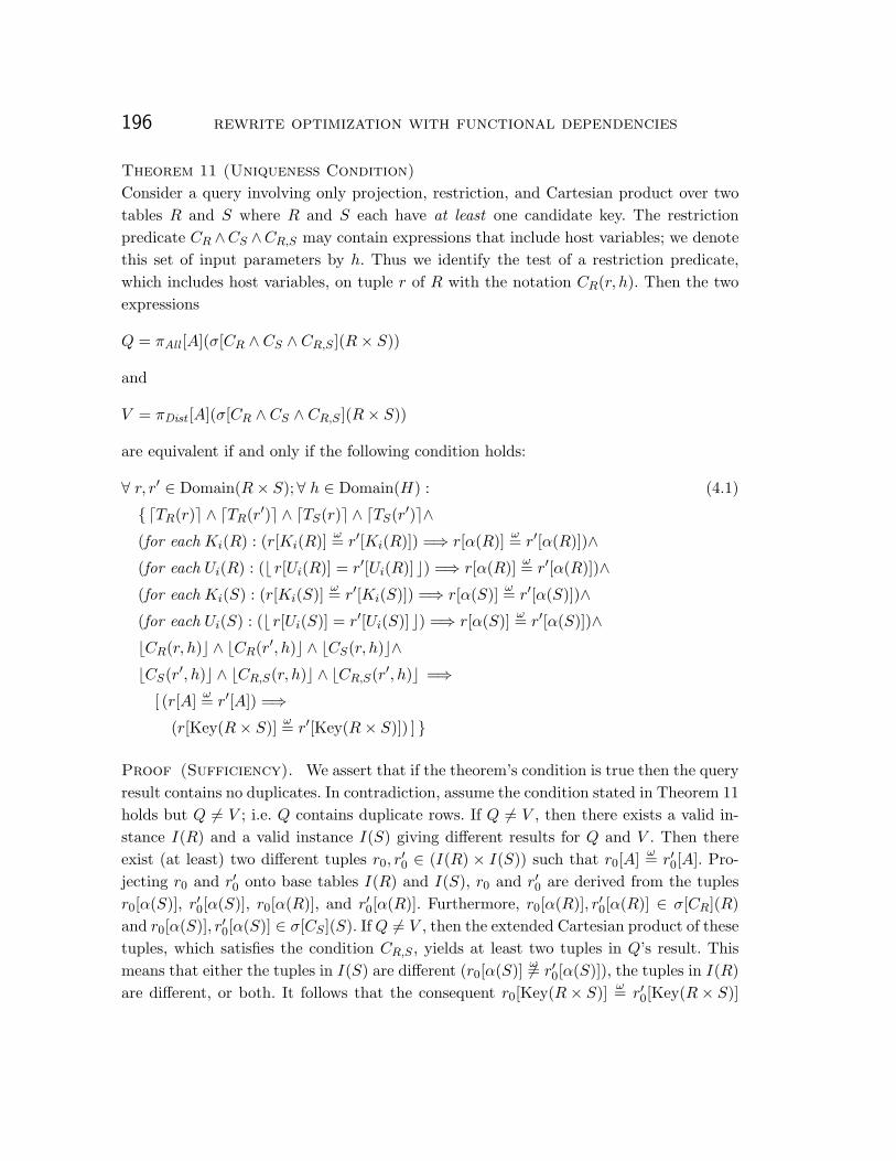
196 rewrite optimization with functional dependencies
Theorem 11 (Uniqueness Condition)
Consider a query involving only projection, restriction, and Cartesian product over twotables R and S where R and S each have at least one candidate key. The restrictionpredicate CR ∧CS ∧CR,S may contain expressions that include host variables; we denotethis set of input parameters by h. Thus we identify the test of a restriction predicate,which includes host variables, on tuple r of R with the notation CR(r, h). Then the twoexpressions
Q = πAll [A](σ[CR ∧ CS ∧ CR,S ](R× S))
and
V = πDist [A](σ[CR ∧ CS ∧ CR,S ](R× S))
are equivalent if and only if the following condition holds:
∀ r, r′ ∈ Domain(R× S);∀ h ∈ Domain(H) : (4.1)
{ �TR(r)� ∧ �TR(r′)� ∧ �TS(r)� ∧ �TS(r′)�∧(for each Ki(R) : (r[Ki(R)]
ω= r′[Ki(R)]) =⇒ r[α(R)] ω= r′[α(R)])∧(for each Ui(R) : (� r[Ui(R)] = r′[Ui(R)] �) =⇒ r[α(R)] ω= r′[α(R)])∧(for each Ki(S) : (r[Ki(S)]
ω= r′[Ki(S)]) =⇒ r[α(S)] ω= r′[α(S)])∧(for each Ui(S) : (� r[Ui(S)] = r′[Ui(S)] �) =⇒ r[α(S)] ω= r′[α(S)])∧�CR(r, h)� ∧ �CR(r′, h)� ∧ �CS(r, h)�∧�CS(r′, h)� ∧ �CR,S(r, h)� ∧ �CR,S(r′, h)� =⇒[ (r[A] ω= r′[A]) =⇒(r[Key(R× S)] ω= r′[Key(R× S)]) ] }
Proof (Sufficiency). We assert that if the theorem’s condition is true then the queryresult contains no duplicates. In contradiction, assume the condition stated in Theorem 11holds but Q �= V ; i.e. Q contains duplicate rows. If Q �= V , then there exists a valid in-stance I(R) and a valid instance I(S) giving different results for Q and V . Then thereexist (at least) two different tuples r0, r′0 ∈ (I(R) × I(S)) such that r0[A]
ω= r′0[A]. Pro-jecting r0 and r′0 onto base tables I(R) and I(S), r0 and r′0 are derived from the tuplesr0[α(S)], r′0[α(S)], r0[α(R)], and r′0[α(R)]. Furthermore, r0[α(R)], r′0[α(R)] ∈ σ[CR](R)and r0[α(S)], r′0[α(S)] ∈ σ[CS ](S). IfQ �= V , then the extended Cartesian product of thesetuples, which satisfies the condition CR,S , yields at least two tuples in Q’s result. Thismeans that either the tuples in I(S) are different (r0[α(S)] �ω= r′0[α(S)]), the tuples in I(R)are different, or both. It follows that the consequent r0[Key(R× S)] ω= r′0[Key(R× S)]

4.2 formal analysis of duplicate elimination 197
must be false, since if either r0[α(S)] �ω= r′0[α(S)], r0[α(R)] �ω= r′0[α(R)], or both, thenthe keys of the respective tuples must be different; a contradiction. Therefore, we con-clude that no duplicate rows can appear in the query result if the condition of Theo-rem 11 holds. ✷
Proof (Necessity). Assume that for every valid instance of the database, Q cannotgenerate any duplicate rows, but the condition stated in Theorem 11 does not hold. Toprove necessity, we must show that we can construct valid instances of R and S for whichQ results in duplicate rows.
If Theorem 11’s condition does not hold, then there must exist two tuples r0, r′0 ∈Domain(R× S) so that the consequent (r0[A]
ω= r′0[A]) =⇒ (r0[Key(R× S)]ω= r′0[Key(R× S)]) is false, but its antecedents (table constraints, key dependencies, andquery predicates) are true. If r0 and r′0 disagree on their key, then there must exist atleast one column ε ∈ Key(R) ◦Key(S) where r[ε] �ω= r′[ε]. Projecting r0 and r′0 onto basetables R and S, we get the database instance consisting solely of the tuples r0[α(S)],r′0[α(S)], r0[α(R)], and r′0[α(R)]. This instance is valid since the tuples satisfy the tableand uniqueness constraints for R and S. Furthermore r0[α(S)], r′0[α(S)] ∈ σ[CS ](S) andr0[α(R)], r′0[α(R)] ∈ σ[CR](R). Because all constraints are satisfied and r0[A]
ω= r′0[A],V contains a single tuple. Suppose ε ∈ Key(S). Then r0[α(S)] �ω= r′0[α(S)], and the ex-tended Cartesian product with r0[α(R)] and r′0[α(R)] satisfying CR,S yields at least twotuples. A similar result occurs if ε ∈ Key(R). In either case, Q contains at least two tu-ples, so Q �= V . Therefore, we conclude that the condition in Theorem 11 is both neces-sary and sufficient. ✷
Note that we can extend this result to involve more than two tables in the Cartesianproduct.
Example 26
Consider the query from Example 25, modified to eliminate duplicate rows:
Select Distinct S.VendorID, S.SupplyCode, P.PartID, P.Description
From Supply S, Part P
Where P.PartID = S.PartID and S.VendorID = :Supplier-No.
We can safely ignore the Distinct specification in the above query if the conditionof Theorem 11 holds:
∀ r, r′ ∈ Domain(S× P);
∀ :Supplier-No ∈ Domain(S.VendorID) :Tuple constraints (Check conditions)
{ �r[P.Price] ≥ r[P.Cost]�∧

198 rewrite optimization with functional dependencies
(�r[P.Qty] �= 0� ∨ �r[P.Status] = Inactive�)∧(�r[S.Rating] = ‘A’� ∨ �r[S.Rating] = ‘B’� ∨ �r[S.Rating] = ‘C’�)∧�r′[P.Price] ≥ r′[P.Cost]�∧(�r′[P.Qty] �= 0� ∨ �r′[P.Status] = Inactive�)∧(�r′[S.Rating] = ‘A’� ∨ �r′[S.Rating] = ‘B’� ∨ �r′[S.Rating] = ‘C’�)∧
Primary key dependency for Supply
(r[S.VendorID] ω= r′[S.VendorID]∧r[S.PartID] ω= r′[S.PartID]) =⇒(r[S.Rating] ω= r′[S.Rating] ∧ r[S.SupplyCode] ω=
r′[S.SupplyCode] ∧ r[S.Lagtime] ω= r′[S.Lagtime])∧Primary key dependency for Part
(r[P.PartID] ω= r′[P.PartID]) =⇒(r[P.Description] ω= r′[P.Description] ∧ r[P.Status] ω= r′[P.Status]∧r[P.Qty] ω= r′[P.Qty] ∧ r[P.Price] ω= r′[P.Price])∧r[P.Cost] ω= r′[P.Cost] ∧ r[P.Support] ω= r′[P.Support])∧r[P.ClassCode] ω= r′[P.ClassCode])∧
Query predicate conditions
�r[S.VendorID] = :Supplier-No� ∧ �r′[S.VendorID] =:Supplier-No� ∧ �r[P.PartID] = r[S.PartID]�∧�r′[P.PartID] = r′[S.PartID]� ] =⇒
Projection attributes
[(r[S.VendorID] ω= r′[S.VendorID] ∧ r[S.SupplyCode] ω=
r′[S.SupplyCode] ∧ r[P.PartID] ω= r′[P.PartID]∧r[P.Description] ω= r′[P.Description]) ] =⇒
Key of P ◦ Key of S
(r[P.PartID] ω= r′[P.PartID] ∧ r[S.PartID] ω= r′[S.PartID]∧r′[S.VendorID] ω= r[S.VendorID])]}
Although complex, this expression is satisfiable: ignoring the table constraints andkey dependencies, we can see from the consequent
(r[S.VendorID] ω= r′[S.VendorID] ∧ r[S.SupplyCode] ω=
r′[S.SupplyCode] ∧ r[P.PartID] ω= r′[P.PartID]∧
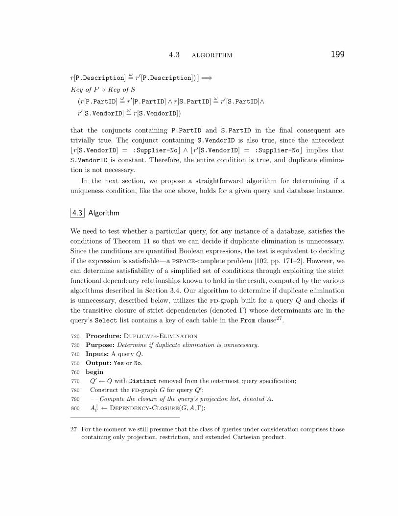
4.3 algorithm 199
r[P.Description] ω= r′[P.Description]) ] =⇒Key of P ◦ Key of S
(r[P.PartID] ω= r′[P.PartID] ∧ r[S.PartID] ω= r′[S.PartID]∧r′[S.VendorID] ω= r[S.VendorID])
that the conjuncts containing P.PartID and S.PartID in the final consequent aretrivially true. The conjunct containing S.VendorID is also true, since the antecedent�r[S.VendorID] = :Supplier-No� ∧ �r′[S.VendorID] = :Supplier-No� implies thatS.VendorID is constant. Therefore, the entire condition is true, and duplicate elimina-tion is not necessary.
In the next section, we propose a straightforward algorithm for determining if auniqueness condition, like the one above, holds for a given query and database instance.
4.3 Algorithm
We need to test whether a particular query, for any instance of a database, satisfies theconditions of Theorem 11 so that we can decide if duplicate elimination is unnecessary.Since the conditions are quantified Boolean expressions, the test is equivalent to decidingif the expression is satisfiable—a pspace-complete problem [102, pp. 171–2]. However, wecan determine satisfiability of a simplified set of conditions through exploiting the strictfunctional dependency relationships known to hold in the result, computed by the variousalgorithms described in Section 3.4. Our algorithm to determine if duplicate eliminationis unnecessary, described below, utilizes the fd-graph built for a query Q and checks ifthe transitive closure of strict dependencies (denoted Γ) whose determinants are in thequery’s Select list contains a key of each table in the From clause27.
Procedure: Duplicate-Elimination720
Purpose: Determine if duplicate elimination is unnecessary.730
Inputs: A query Q.740
Output: Yes or No.750
begin760
Q′ ← Q with Distinct removed from the outermost query specification;770
Construct the fd-graph G for query Q′;780
– –Compute the closure of the query’s projection list, denoted A.790
A+Γ ← Dependency-Closure(G,A,Γ);800
27 For the moment we still presume that the class of queries under consideration comprises thosecontaining only projection, restriction, and extended Cartesian product.

200 rewrite optimization with functional dependencies
if any element of A+Γ is a tuple identifier vertex then810
return Yes820
else830
return No840
fi850
end860
4.3.1 Simplified algorithm
While an fd-graph can be used to determine whether or not duplicate elimination is un-necessary, it is possible to optimize a slightly smaller class of queries by using a simpli-fied form of fd-graph than that presented earlier. Our proposed algorithm exploits infor-mation about primary keys, candidate keys, and equality conditions in a Where clause.As with the analysis of restriction predicates in Section 3.2.4, we classify equality condi-tions into two types: Type 1 of the form (v = c) and Type 2 of the form (v1 = v2) wherev, v1, v2 are columns and c is a constant.
Our simplified algorithm, Simplified-Duplicate-Elimination, uses a simplifiedform of fd-graph that does not require tuple identifiers, lax dependency edges, outer joinvertices and edges, or equivalence edges. The algorithm requires the infrastructure to sup-port only base tables, extended Cartesian product, and restriction. We first construct ahypergraph consisting of all of the base tables in the query’s From clause, using a simpli-fied version of the Base Table algorithm, which builds a hypergraph representing thefunctional dependencies that hold for a base table’s primary and definite candidate keys.
Procedure: Base-table (simplified)870
Purpose: Construct a simplified FD-graph for table R.880
Inputs: scheme of table R; query Q.890
Output: fd-graph G.900
begin910
for each attribute ai ∈ AR do920
Construct vertex vi ∈ V A;930
Colour[vi]← Black;940
if ai is nullable in R then950
Nullability[vi]← Nullable960
else970
Nullability[vi]← Definite980
fi990
od ;1000
for each primary or candidate key of R do1010

4.3 algorithm 201
if ∃ any key column that is nullable then continue fi ;1020
if Key(R) is composite then1030
Construct the composite vertex K;1040
V C ← V C ∪K;1050
for each v ∈ K do1060
EC ← EC ∪ (K, v)1070
od1080
else1090
Let K denote the singleton key vertex K ∈ V A1100
fi1110
for each v ∈ V A such that v �∈ K do1120
EF ← EF ∪ (K, v)1130
od1140
od ;1150
for each attribute ai ∈ AR referred to in the Select list of Q do1160
Colour[vi]← White1170
od1180
return G1190
end1200
Construction of the simplified fd-graph to determine if a uniqueness condition holdsconsists of three steps. First, we union the base-table fd-graphs together (as usual, we as-sume that all attributes can be uniquely identified by their correlation names). Second,we add strict functional dependency edges to G for each Type 1 and Type 2 equality con-dition in the query’s Where clause28. The algorithm supports only a simplified set of com-parison conditions: conjunctive, null-intolerant equality conditions of Type 1 or 2, withno support for scalar functions. Third, we utilize the Dependency-Closure algorithmto compute the transitive closure of the white attributes in G (the attributes in the pro-jection) and then determine if the closure covers a primary or candidate key from eachtable.
Algorithm: Simplified-Duplicate-Elimination1210
Purpose: Determine if duplicate elimination is unnecessary.1220
Inputs: predicates CR, CS , CR,S ; key constraints U(R), U(S),K(R),K(S); projection list A.1230
Output: Yes or No.1240
begin1250
– –Construct an FD-graph for the query’s extended Cartesian product.1260
28 As with the algorithms in Chapter 3, we assume a priori that each Where clause, if necessary,has been converted to conjunctive normal form.

202 rewrite optimization with functional dependencies
G← ∅;1270
for each table Ti in the From clause (the set {R,S}) do1280
G← G∪ simplified-base-table(Ti);1290
od1300
– –Construct strict edges for search conditions in the Where clause.1310
Separate CR ∧ CS ∧ CR,S ∧ T into conjuncts: C ′ = P1 ∧ P2 ∧ . . . ∧ Pn;1320
for each Pi ∈ C ′ do1330
if Pi contains an atomic condition not of Type 1 or Type 2 then delete Pi from C ′1340
else if Pi contains a disjunctive clause then delete Pi from C ′ fi fi1350
od1360
for each conjunctive predicate Pi ∈ C ′ do1370
– –Consider Type 1 conditions that equate an attribute to a constant.1380
if Pi is a Type 1 condition (v = c) then1390
Construct vertex χ(c) to represent the constant c;1400
V [G]← V [G] ∪ χ(c);1410
Colour[χ(c)] ← Gray;1420
Nullability[χ(c)]← Definite;1430
EF ← EF ∪ (χ(v), χ(c));1440
EF ← EF ∪ (χ(c), χ(v))1450
else1460
– –Consider Type 2 conditions in Pi.1470
if Pi is a Type 2 condition (v1 = v2) then1480
EF ← EF ∪ (χ(v1), χ(v2));1490
EF ← EF ∪ (χ(v2), χ(v1))1500
fi1510
fi1520
od1530
A+Γ ← dependency-closure(G,A,Γ);1540
for each table Ti ∈ Q do1550
if any candidate Key((Ti)) ∈ A+Γ then continue1560
else1570
return No1580
fi1590
od1600
return Yes1610
end1620

4.3 algorithm 203
S.PartID
VendorIDVendorIDS.PartID Supply
Code
(a) Simplified fd-graph for supply.
P.PartID
Description
(b) Simplified fd-
graph for part.
S.PartID
VendorIDVendorIDS.PartID Supply
Code
:Supplier-No
P.PartID
Description
(c) Simplified fd-graph for
Select Distinct S.VendorID, S.SupplyCode, P.PartID, P.Description
From Supply S, Part P
Where P.PartID = S.PartID and S.VendorID = :Supplier-No.
Figure 4.1: Development of a simplified fd-graph for the query in Example 26.

204 rewrite optimization with functional dependencies
Example 27
Suppose we are given the query of Example 26:
Select Distinct S.VendorID, S.SupplyCode, P.PartID, P.Description
From Supply S, Part P
Where P.PartID = S.PartID and S.VendorID = :Supplier-No.
Applying simplified-duplicate-elimination to this query we can trace the followingsteps:
Line 1290: The simplified fd-graphs for the base tables part and supply are shown inFigure 4.1. The strict functional dependencies in each graph correspond to the pri-mary keys of each table. The simplified fd-graph that represents the Cartesian prod-uct of these two tables is the union of the vertices and edges of these two graphs.
Line 1320: C ′ ⇐⇒ S.VendorID = :Supplier-No ∧ S.PartID = P.PartID ∧T .
Lines 1330–1360: C ′ is unchanged.
Line 1410: Here a vertex representing the unknown constant in the host variable:Supplier-No is added to the graph, as are two strict edges between it and thevertex representing S.VendorID.
Line 1480: At this point we add two other strict edges to the graph between the twoexisting vertices that represent S.PartID and P.PartID. At this point no furtheredges are to be added, and the resulting fd-graph is shown in Figure 4.1(c).
Line 1540: Executing the dependency-closure algorithm on the simplified fd-graphG, which embodies the set of strict functional dependencies Γ, yields A+
Γ = {S.VendorID, S.SupplyCode, P.PartID, P.Description, S.PartID }.
Line 1560: A+Γ contains both the primary key of part (P.PartID) and the primary key
of supply ({ S.VendorID, S.PartID } ); we proceed.
Line 1610: Return Yes and stop.
Since the algorithm returns Yes, we know that the Distinct clause in the query is un-necessary.

4.4 applications 205
4.3.2 Proof of correctness
Algorithm simplified-duplicate-elimination tests a simpler, sufficient condition thanthat stated in Theorem 11; it ignores table constraints TR and TS and considers onlyconjunctive, atomic equality conditions in the query’s Where clause. Any Pi deleted online 1340 weakens condition C, but C remains a sufficient condition for testing if dupli-cate elimination is unnecessary. Similarly, any Pi deleted on line 1350 removes conditionslike ‘X = 5 or X = 10’. Therefore, we need to show that the simplified condition
∀ r, r′ ∈ Domain(R× S);∀ h ∈ Domain(H) : (4.2)
(for each Ki(R) : (r[Ki(R)]ω= r′[Ki(R)]) =⇒ r[α(R)] ω= r′[α(R)])∧
(for each Ki(S) : (r[Ki(S)]ω= r′[Ki(S)]) =⇒ r[α(S)] ω= r′[α(S)])∧
�CR(r, h)� ∧ �CR(r′, h)� ∧ �CS(r, h)�∧�CS(r′, h)� ∧ �CR,S(r, h)� ∧ �CR,S(r′, h)� =⇒[ (r[A] ω= r′[A]) =⇒(r[Key(R× S)] ω= r′[Key(R× S)]) ] }
where C ′R, C
′S , and C ′
R,S contain only atomic conditions using ‘=’, is true when the al-gorithm returns Yes. Assuming simplified-duplicate-elimination returns Yes, con-sider one iteration of the main loop starting on line 1370. Since line 1560 yields True (theprimary keys of both R and S occur in Γ+), then we know that the Key(R) ◦ Key(S)is functionally determined from the result attributes; a derived functional dependency.This means that the consequent (r[A] ω= r′[A]) =⇒ (r[Key(R× S)] ω= r′[Key(R× S)])must be true. Since we assume that all key dependencies hold, and we considered onlyconjunctive components Pi ∈ C ′ then the simplified condition must hold for C sinceP1 ∧ P2 ∧ . . . ∧ Pm ⇐⇒ C ′
R ∧ C ′S ∧ C ′
R,S .
4.4 Applications
Our goal is to show how relational query optimizers can employ Theorem 11 to expandthe space of possible execution strategies for a variety of queries. Once the optimizer iden-tifies possible transformations, it can then choose the most appropriate strategy on thebasis of its cost model. In this section, we identify four important query transformations:detection of unnecessary duplicate elimination, conversion of a subquery to a join, conver-sion of set intersection to a subquery, and conversion of set difference to a subquery. Otherresearchers have described these query transformations elsewhere [74, 157, 212, 230] butwith relatively little formalism. Later, in Section 6.2, we show the applicability of thesetransformations in nonrelational environments.

206 rewrite optimization with functional dependencies
4.4.1 Unnecessary duplicate elimination
We believe that many queries contain unnecessary Distinct clauses, for two reasons.First, case tools often generate queries using ‘generic’ query templates. These templatesspecify Distinct as a conservative approach to handling duplicate rows. Second, somepractitioners [71] encourage users to always specify Distinct, again as a conservative ap-proach to simplify query semantics. We feel that recognizing redundant Distinct clausesis an important optimization, since it can avoid a costly sort.
Example 28
Consider the following query which lists the vendor id and part data for every part sup-plied by a vendor with the name :VendorName:
Select Distinct V.VendorID, P.PartID, P.Description, P.Qty
From Supply S, Vendor V, Part P
Where V.Name = :VendorName and V.VendorID = S.VendorID
and S.PartID = P.PartID.
This query satisfies the conditions in Theorem 11, and, consequently, Distinct in theSelect clause is unnecessary.
4.4.2 Subquery to join
A number of researchers over the years, including Kim [157], Ganski and Wong [101],Muralikrishna [211, 212], Dayal [74], Pirahesh, Hellerstein, and Hasan [230], and Steen-hagen, Apers, and Blanken [265] have studied the rewriting of correlated, positive exis-tential subqueries as joins. Their rationale is to avoid processing the query with a naivenested-loop strategy. Instead, they convert the query to a join so that the optimizer canconsider alternate join methods.
The class of queries we consider corresponds to Type j nested queries in Kim’s paper;however, we explicitly consider three-valued logic and duplicate rows. Pirahesh et al. con-sider merging existential subquery blocks in Rule 7 of their suite of rewrite rules in thestarburst query optimizer. We believe that it is worthwhile to analyze several subquery-to-join transformations, particularly when duplicate rows are permitted.
Example 29
Consider the correlated query

4.4 applications 207
Select All Q.QuoteID, Q.Date, Q.QtyPrice
From Quote Q
Where Q.MinOrder > :Minimum-Qty and
Exists (Select *
From Part P
Where Q.PartID = P.PartID and
P.PartID = :Part-No)
which lists all part quotations for a given part (from all the part’s suppliers) as long asthe minimum order quantity in the quote is greater than the parameter ‘Minimum-Qty’,which is a host variable. We claim that this query may be rewritten as
Select All Q.QuoteID, Q.Date, Q.QtyPrice
From Quote Q, Part P
Where Q.MinOrder > :Minimum-Qty and
Q.PartID = P.PartID and
P.PartID = :Part-No
since the conditions in the subquery block can, at most, identify a single tuple in thepart table for each candidate tuple in quote.
Theorem 12 (Subquery to Join)
Consider a nested query on tables R and S that contains a positive existential subqueryblock. Assume that R and S have at least one candidate key and the same preconditionsfor host variables, as described in Theorem 11, hold. Then the two expressions
Q = πAll [AR](σ[CR ∧ ∃(σ[CS ∧ CR,S ](S))](R))
and
V = πAll [AR](σ[CR ∧ CS ∧ CR,S ](R× S))
are equivalent if and only if the following condition holds:
∀ r ∈ Domain(R); ∀ h ∈ Domain(H) : (4.3)
{ [ �TR(r)� ∧ �CR(r, h)� ] =⇒[ [∀ s, s′ ∈ Domain(S) :�TS(s)� ∧ �TS(s′)�∧(for each Ki(S) : (s[Ki(S)]
ω= s′[Ki(S)]) =⇒ s[α(S)] ω= s′[α(S)])∧(for each Ui(S) : (� s[Ui(S)] = s′[Ui(S)] �) =⇒ s[α(S)] ω= s′[α(S)])∧�CS(s, r, h)� ∧ �CS(s′, r, h)� ∧ �CR,S(s, r, h)� ∧ �CR,S(s′, r, h)� ] =⇒(s[RowID(S)] ω= s′[RowID(S)]) ] }

208 rewrite optimization with functional dependencies
Proof (Sufficiency). We assert that at most one tuple from S can match the restric-tion predicate CS ∧ CR,S if the condition in Theorem 12 holds. We prove this claim bycontradiction; assume the condition in Theorem 12 holds, but the expressions Q and V
are not equivalent. Then there must exist instances I(R) and I(S), a tuple r0 ∈ I(R), and(at least) two different tuples s0, s
′0 ∈ I(S) such that CS(s0, h), CS(s′0, h), CR,S(r0, s0, h),
and CR,S(r0, s′0, h) are satisfied. Since all the antecedents in the condition hold, and thetable and key constraints hold for every tuple in Domain(R× S), then s0 and s′0 mustagree on their key. However, if the two tuples s0 and s′0 agree on their key, then they vi-olate the candidate key constraint for S, a contradiction.
We now argue that the semantics of Q and V are equivalent if at most one tuple fromS matches each tuple from R. If the predicate CS ∧ CR,S in Q is false or unknown, thenthe existential predicate ∃(σ[CS ∧CR,S ](S)) must return false, and the tuple representedby r0 cannot be part of the result. Otherwise, if CS ∧ CR,S is true then r0 appears inthe result. Similarly, for query V , any tuple r0 that satisfies CR will join with at mostone tuple s0 of S if the condition in Theorem 12 holds. If CS ∧ CR,S is false or unknownfor the two tuples r0 and s0 the restriction predicate is false; hence r0 will not appear inthe result. If CS ∧ CR,S is true then at most one tuple of S qualifies, and the extendedCartesian product produces only a single tuple from R. Therefore, if at most one tuplefrom S matches each tuple of R, then Q = V . ✷
Proof (Necessity). Assume that for every valid instance of the database, the sub-query block on S can match at most one tuple r of R but the condition in Theorem 12does not hold. To prove necessity, we must show we can construct valid instances I(R)and I(S) so that evaluating Q and V on those instances yields a different result.
If the condition in Theorem 12 is false there must exist two different tuples s0, s′0 ∈
Domain(S) and a tuple r0 ∈ Domain(R) such that the consequent (s0[Key(S)]ω=
s′0[Key(S)]) is false, but its antecedents are true. The instance of S formed by tuples s0
and s′0 is certainly valid, since it satisfies the table and uniqueness constraints for I(S).In turn, r0 is a valid instance of R because it satisfies the constraints on R. Since r0 satis-fies the condition CR and since both s0 and s′0 satisfy the restriction predicate CS ∧CR,S ,then Q yields one instance of r0 in the result, but V yields two, a contradiction. We con-clude that the condition in Theorem 12 is both necessary and sufficient. ✷
At this point, we can make several observations. Trivially, if the subquery in Q in-cludes more than one table so that the subquery involves an extended Cartesian productof, say, tables S and W , we can extend Theorem 12 to include the corresponding condi-tions of W (similar to Theorem 11). Moreover, we observe that the two expressions
Q = πDist [AR](σ[CR ∧ ∃(σ[CS ∧ CR,S ](S))](R))

4.4 applications 209
and
V = πDist [AR](σ[CR ∧ CS ∧ CR,S ](R× S))
are always equivalent, since duplicate elimination in the projection automatically ex-cludes duplicate tuples obtained from the Cartesian product if more than one tuple in Smatches the restriction predicate. This means that if we can alter the projection πAll [AR]to πDist [AR] without changing the query’s semantics, then we can always convert a nestedquery to a join, as illustrated by the following example.
Example 30
Consider the correlated query
Select All V.VendorID, V.Name, V.Address
From Vendor V
Where Exists (Select *
From Part P, Supply S, Quote Q
Where P.PartID = S.PartID and V.VendorID = S.VendorID
and Q.PartID = P.PartID and Q.VendorID = S.VendorID
and Q.MinOrder < 500 and P.Qty > 1000 )
which lists all suppliers who supply at least one part that is significantly overstocked,but whose minimum order quantity has been less than 500. Note that the uniquenesscondition does not hold on the subquery block since many quotes can exist for the samepart sold by the same vendor. However, this query may be rewritten as
Select Distinct V.VendorID, V.Name, V.Address
From Vendor V, Part P, Supply S, Quote Q
Where P.PartID = S.PartID and V.VendorID = S.VendorID
and Q.PartID = P.PartID and Q.VendorID = S.VendorID
and Q.MinOrder < 500 and P.Qty > 1000
since the uniqueness condition is satisfied for the outer query block (VendorID is the keyof vendor). The optimizer converts the query to a join, disregards any columns from theother tables in the From clause, and then applies duplicate elimination that outputs onlyone vendor tuple for each unique VendorID in the Cartesian product. This observationleads to the following corollary:
Corollary 3 (Subquery to Distinct Join)
Consider a nested query on tables R and S that contains a positive existential subqueryblock. Assume that R and S have at least one candidate key and the same preconditionsfor host variables, as described in Theorem 12, hold. Then the two expressions
Q = πAll [AR](σ[CR ∧ ∃(σ[CS ∧ CR,S ](S))](R))

210 rewrite optimization with functional dependencies
and
V = πDist [AR](σ[CR ∧ CS ∧ CR,S ](R× S))
are equivalent if πAll [AR](σ[CR](R)) contains no duplicate rows. Duplicate eliminationin the projection can be implemented through the use of tuple identifier(s) if suitableprimary keys are either missing or are absent from the projection list [AR].
Two additional, though perhaps straightforward, observations are noteworthy here.First, note that we can safely transform a Select Distinct to a Select All in anysubquery that is involved in a set-oriented search condition (e.g. In, Any, All, Some).This is because the select list of any Exists subquery is of no consequence to its result,and can be replaced by a simple literal29. We cannot, however, safely ignore Distinct ina subquery that is part of a scalar theta-comparison, since the rdbms must generate arun-time execution error if the subquery returns more than one row.
Second, note that once all set-oriented predicates involving nested subqueries (e.g.In, Any, All, Some) have been transformed to simple (correlated) Exists predicateswe can always flatten nested spj queries into joins without the need for duplicate elimi-nation as long as the query’s outermost block is not involved—that is, the subquery be-ing ‘flattened’ is itself contained within another subquery. This is (again) because the se-lect list of any Exists subquery is of no consequence to its result, so retaining duplicatetuples will not affect the result of any Exists predicate.
Thus far we have proved the equivalence of nested queries and joins in a variety of sit-uations. Commercial relational database systems exploit this equivalence to transformnested queries to joins whenever possible [230] so that their optimizers’ join enumerationalgorithms can try to construct a less expensive access plan. To our knowledge, no com-mercial rdbms performs the reverse transformation: rewriting a join as a subquery as asemantic transformation. Later, in Section 6.2, we consider this opposite case and show itspotential as a semantic optimization in different database environments, including hier-archical and object-oriented database systems. For now, we present examples where con-verting an sql query expression—specifically those involving Except or Intersect—intoa nested query specification could lead to a cheaper access plan.
29 In fact, the ansi standard defines Exists subqueries in precisely this manner.

4.4 applications 211
4.4.3 Distinct intersection to subquery
Typically, most relational query optimizers execute the Intersect operation by evaluat-ing each operand, sorting each intermediate result if necessary, and merging the inputs.Recall that the semantics of Intersect requires ignoring duplicates and, more trouble-some, equating two tuples if:
• all non-Null columns are equal and
• for each Null column, its counterpart in the other (derived) table is also Null.
A subtle difficulty with the transformation of query expressions to nested query specifi-cations arises because the equivalence of tuples, normally handled by a set operator thattreats null values as equivalent, is now moved into a Where clause. Pirahesh et al. [230]do not handle this situation adequately in their paper (Rule 8); they transform a querywithout considering possibly Null keys.
Theorem 13 (Distinct Intersection to Exists)
Consider a query expression that contains the set intersection operator on two tables Rand S where R and S each have at least one candidate key. Either restriction predicateCR(R) or CS(S) may contain host variables. Then the two expressions
Q = πAll [AR](σ[CR](R)) ∩Dist πAll [AS ](σ[CS ](S))
and
V = πAll [AR](σ[CR ∧ ∃(σ[CS ∧ CR,S ](S))](R)),
where CR,S =∧m
i=1 R[Ai]ω= S[Ai] are equivalent if the derived table πAll [AR](σ[CR](R))
does not contain duplicate rows.
Proof. Omitted. ✷
Recall that the semantics of R ∩Dist S are to include a tuple from R iff it exists inS, and eliminate any duplicates in the result. If each result tuple from R is unique, thena tuple from πAll [AR](σ[CR](R)) may appear in the final result if at least one matchingtuple is found in πAll [AS ](σ[CS ](S)).
Observe that the predicate CR,S =∧m
i=1 R[Ai]ω= S[Ai] can be expressed in sql as
(R.X Is Null and S.X Is Null) or R.X = S.X for each attribute X in the projectionlist (though a plain equijoin predicate will suffice for primary key columns, since a pri-mary key is guaranteed not to contain any Null values). Using a primary key makes thetransformation in Example 5 of reference [230] correct.
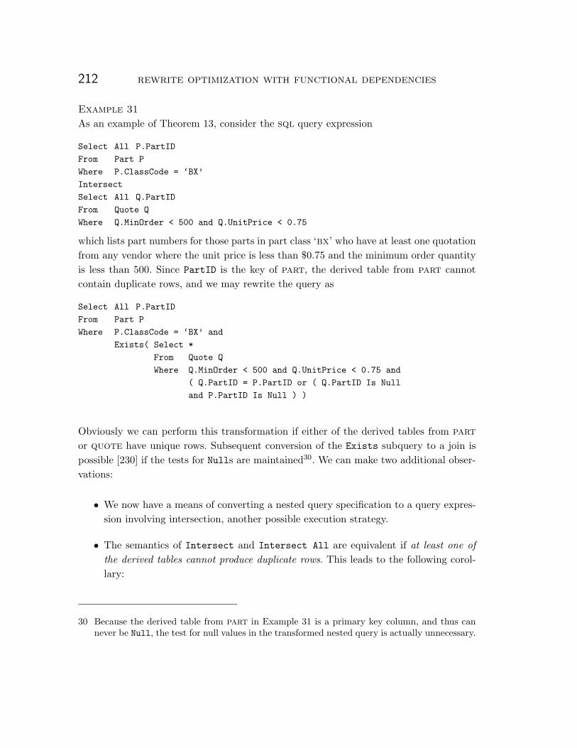
212 rewrite optimization with functional dependencies
Example 31
As an example of Theorem 13, consider the sql query expression
Select All P.PartID
From Part P
Where P.ClassCode = ‘BX’
Intersect
Select All Q.PartID
From Quote Q
Where Q.MinOrder < 500 and Q.UnitPrice < 0.75
which lists part numbers for those parts in part class ‘bx’ who have at least one quotationfrom any vendor where the unit price is less than $0.75 and the minimum order quantityis less than 500. Since PartID is the key of part, the derived table from part cannotcontain duplicate rows, and we may rewrite the query as
Select All P.PartID
From Part P
Where P.ClassCode = ‘BX’ and
Exists( Select *
From Quote Q
Where Q.MinOrder < 500 and Q.UnitPrice < 0.75 and
( Q.PartID = P.PartID or ( Q.PartID Is Null
and P.PartID Is Null ) )
Obviously we can perform this transformation if either of the derived tables from partor quote have unique rows. Subsequent conversion of the Exists subquery to a join ispossible [230] if the tests for Nulls are maintained30. We can make two additional obser-vations:
• We now have a means of converting a nested query specification to a query expres-sion involving intersection, another possible execution strategy.
• The semantics of Intersect and Intersect All are equivalent if at least one ofthe derived tables cannot produce duplicate rows. This leads to the following corol-lary:
30 Because the derived table from part in Example 31 is a primary key column, and thus cannever be Null, the test for null values in the transformed nested query is actually unnecessary.

4.4 applications 213
Corollary 4 (All Intersection to Exists)
Consider a query expression that contains the set operator Intersect All. Assume thatR and S have at least one candidate key, and the same preconditions for host variables,as described in Theorem 11, hold. Then the two expressions
Q = πAll [AR](σ[CR](R)) ∩All πAll [AS ](σ[CS ](S))
and
V = πAll [AR](σ[CR ∧ ∃(σ[CS ∧ CR,S ](S))](R)),
where CR,S is defined as in Theorem 13 are equivalent if the expression πAll [AR](σ[CR](R))does not contain duplicate rows. Similarly, Q and V (modified by interchanging R andS) are equivalent if the query specification on S does not contain duplicate rows.
4.4.4 Set difference to subquery
In a manner similar to the typical computation of set intersection, which sorts the two in-puts and performs a merge, sql’s two set difference operators are typically processedby sorting the two operands and subsequently computing the difference of the two tu-ple streams. However, the semantics of set difference offers a natural transformation toa nested query form containing a Not Exists predicate, which can offer additional op-timization opportunities. Once again, we have to be careful about the possible existenceof null values in order to ensure a correct result.
Example 32
Consider the sql query expression
Select Distinct P.PartID
From Part P
Where P.ClassCode = ‘BX’
Except All
Select Distinct S.PartID
From Supply S
which lists part numbers for those parts in part class ‘bx’ that are not supplied by anysupplier. Since PartID is the key of part, the derived table from part cannot containduplicate rows, and we may rewrite the query as

214 rewrite optimization with functional dependencies
Select All P.PartID
From Part P
Where P.ClassCode = ‘BX’ and
Not Exists( Select *
From Supply S
Where ( S.PartID = P.PartID or ( S.PartID Is Null
and S.PartID Is Null ) ).
Note that because PartID cannot be Null in either table, the disjunction that testsfor Null can be omitted. Note as well that we may hereafter utilize Dayal’s [74] tech-niques to convert this negated Exists predicate into an outer join—more precisely, to agrouped query over an outer join with a Having clause containing the aggregate func-tion Count(*)—which offers yet another syntactic form that could lead to a more effi-cient access plan.
Example 32 illustrates three separate transformations. The first is to rewrite the queryexpression involving Except All as a nested query. This is possible because the Distinctin the first query specification means that there cannot be any duplicate rows in the re-sult; hence in this case Except and Except all computes the identical result. To com-pute the result utilizing the nested query, we need only verify that each qualifying PartIDfrom part does not exist in any row of supply. Second, note that the Distinct in thesecond query specification is unnecessary since we are implementing the semantics ofExcept—duplicate tuples in the subquery do not affect the output. Third, we can elim-inate the Distinct from the outer block in the nested query since PartID is the key ofpart and hence there cannot be duplicate parts in the output.
More formally, we state the equivalence of these two queries as follows:
Lemma 35 (Except all to Except)
Consider a query expression that contains the set difference operator on two tables R andS where R and S each have at least one candidate key (an actual key or tuple identifier).Either restriction predicate CR(R) or CS(S) may contain host variables. Then the twoexpressions
Q = πAll [AR](σ[CR](R))−All πAll [AS ](σ[CS ](S))
and
V = πAll [AR](σ[CR](R))−Dist πAll [AS ](σ[CS ](S))
are equivalent iff the derived table πAll [AR](σ[CR](R)) does not contain duplicate rows.
Proof. Straightforward from the definition of Except all. ✷

4.5 related work 215
Theorem 14 (Distinct Difference to Not Exists)
Consider a query expression that contains the set difference operator on two tables Rand S where R and S each have at least one candidate key. Either restriction predicateCR(R) or CS(S) may contain host variables. Then the two expressions
Q = πAll [AR](σ[CR](R))−All πDist [AS ](σ[CS ](S))
and
V = πAll [AR](σ[CR ∧ � ∃(σ[CS ∧ CR,S ](S))](R)),
where CR,S =∧m
i=1 R[Ai]ω= S[Ai] are equivalent if the derived table πAll [AR](σ[CR](R))
does not contain duplicate rows.
Proof. Omitted. ✷
4.5 Related work
Semantic transformation of sql queries using our uniqueness condition is a form of seman-tic query optimization [161]. Kim [157] originally suggested rewriting correlated, nestedqueries as joins to avoid nested-loop execution strategies. Subsequently, several researcherscorrected and extended Kim’s work, particularly in the aspects of grouping and aggrega-tion [47, 74, 101, 155, 211, 212]. Much of the earlier work in semantic transformations ig-nored sql’s three-valued logic and the presence of Null values. To help better understandthese problems, Negri, Pelagatti, and Sbattella [216] and von Bultzingsloewen [288] de-fined formal semantics for sql using an extended relational calculus, although neither pa-per tackled the problems of duplicates. A significant contribution of Negri et al. is theirnotion of query equivalence classes for syntactically different, yet semantically equiva-lent, sql queries.
Several authors discuss the properties of derived functional dependencies in two-valuedlogic. Klug [162] studied the problem of derived strict dependencies in two-valued re-lational algebra expressions with the operators projection, selection, restriction, cross-product, union, and difference. His paper’s main contributions were (1) the problem ofdetermining the equivalence of two arbitrary relational expressions is undecidable, (2)the definition and proof of a transitive closure operator for strict functional dependen-cies, and (3) an algorithm to derive all strict functional dependencies for an arbitrary ex-pression, without set difference, and with a restricted order of algebraic operators. Maier[193] describes query modification techniques with respect to minimizing the number ofrows in tableaux, which is equivalent to minimizing the number of joins in relational al-gebra. Maier’s chase computation uses functional and join dependencies to transform

216 rewrite optimization with functional dependencies
tableaux. Darwen [70] reiterates Klug’s work, and gives an exponential algorithm for gen-erating derived strict functional dependencies. Darwen concentrates on deriving candi-date keys for arbitrary algebraic expressions and their applications, notably view updata-bility and join optimization. Ceri and Widom [48] discuss derived key dependencies withrespect to updating materialized views. They define these dependencies in terms of an al-gorithm for deducing bound columns, quite similar in purpose to our simplified-dupli-cate-elimination algorithm. In our approach, however, our formal proofs take into ac-count other static constraints and explicitly handle the existence of Null values; our al-gorithm is simply a sufficient condition for determining candidate keys.
Pirahesh, Hellerstein, and Hasan [230] draw parallels between optimization of sqlsubqueries in relational systems and the optimization of path queries in object-orientedsystems. Their work in starburst focuses on rewriting complex Select statements asselect-project-join queries. One of the query rewrite rules identifies when duplicate elim-ination is not required, through isolation of two conditions: uniqueness, termed the ‘one-tuple-condition’, and existence of a primary key in a projection list, termed the ‘quantifier-nodup-condition’. However, we feel that optimization opportunities may be lost upontheir insistence that the starburst rewrite engine convert all queries, whenever possi-ble, to joins. In contrast, we believe that converting joins to subqueries offers possibilitiesfor optimization in nonrelational systems. We explore that possibility in Chapter 6.
Bhargava, Goel and Iyer [32–34] extended the work described in this chapter and ap-plied it to the optimization of (a) outer joins and (b) the set operators Union, Inter-sect, and Except and their interaction with projections of query specifications that elim-inate duplicates. Their research into outer join optimization covered (1) join eliminationof an outer join in the presence of distinct projection, (2) simplifications of outer joinsto inner joins, (3) discovery of a uniqueness condition for a query block containing (pos-sibly nested) outer joins. Their approach to uniqueness conditions with respect to outerjoins was based on key sets, and influenced our approach to the maintenance of lax de-pendencies in fd-graphs. Some of their later work on set operations mirrors our own re-search, which due to space constraints was omitted from publication [228].
4.6 Concluding remarks
We have formally proved the validity of a number of semantic query rewrite optimiza-tions for a restricted set of sql queries, and shown that these transformations can poten-tially improve query performance in both relational and nonrelational database systems.Although testing the conditions for transformation is pspace-complete, our algorithm de-tects a large subclass of queries for which the transformations are valid. Our approach

4.6 concluding remarks 217
takes into account static constraints, as defined by the sql2 standard, and explicitly han-dles the ‘semantic reefs’ [155] referred to by Kiessling—duplicate rows and three-valuedlogic—which continue to complicate optimization strategies.


5 Tuple sequences and functional dependencies
An obvious benefit of using an ordered data structure like a b+-tree in the implementa-tion of a relational database system is that tuples may be retrieved in ascending or de-scending secondary key sequence, which quite often matches the ordering of the resulttuples desired by an application program. Indexes present one of the few opportunitiesfor exploiting ordering since tuples in base tables are not typically maintained in key se-quence (clustered indexes are one exception). In this chapter, we illustrate how we canexploit tuple sequences [2, 3] in optimizing queries over ansi sql relational databases. Inaddition to project-select-join queries we formally defined in Section 2.3, we will also lookat the possibility of exploiting tuple sequences to compute the result of sql query spec-ifications containing Group by, and query expressions containing Union or Union all,Intersect or Intersect all, and Except or Except all. Throughout this section, forsimplicity we assume that the domains of attributes involved in any query can be to-tally ordered [103].
5.1 Possibilities for optimization
Example 33
Consider the sql query
Select D.Name, E.Surname, E.GivenName, E.Phone
From Division D, Employee E
Where D.Name = E.DivName
Order by E.Surname
that lists information about each employee in the firm in ascending sequence by surname,using the manufacturing schema described in Appendix A.
There are several possible ways to process the above query (see Figure 5.1). One pos-sible access strategy, shown in Figure 5.1(a), is to perform a sort-merge join of the twotables over Name and Divname. Given the lack of any other restriction predicate, it maybe necessary to first sort both the division and employee tables in their entirety, per-form the merge join, and then sort the join’s output to satisfy the Order by clause. Sorts
219

220 tuple sequences and functional dependencies
of the input relations could be avoided if there exist the appropriate indexes on each ta-ble, though retrieving each tuple randomly through the index is likely to significantly in-crease the cost of retrieval.
A second possible strategy (b) is to perform an indexed nested-loop join with thedivision as the ‘outer’ table, and employee as the indexed ‘inner’, assuming an indexon the Divname attribute of employee. Conversely, strategy (c) reverses the join orderand scans employee as the ‘outer’ table. In either case, however, we will need to sortthe entire result to satisfy the query’s Order by clause. However, suppose there existsan ascending index on Surname. Then a fourth possible strategy (d) is to scan the outeremployee table by the index on Surname, and join each employee tuple with at mostone from division as before. In this case a final sort of the result would be unnecessary,assuming that the nested-loop join implementation is order-preserving.
The process of query optimization is responsible for analyzing these tradeoffs to de-termine the cheapest access plan. Because every employee tuple will be in the result,the most efficient way to retrieve them is to perform a sequential scan. However, this ac-cess strategy requires a final sort, so it may not be the cheapest overall. Furthermore, itis not possible to return any result tuples to the application until all the employee tu-ples have been retrieved.
Using strategy (d), though possibly more costly, avoids both of these problems. Thisstrategy may be particularly appropriate if only a subset of the tuples in the result willactually be retrieved by the application [42–44]. But this strategy will not always be con-sidered in a commercial database system. For example, the query optimizer in oracleVersion 7 rejects outright such a strategy as too expensive [69]. oracle will exploit an in-dex to satisfy an Order by clause only if there exists at least one restriction predicate onthe index’s secondary key (in this case, Surname).
In this chapter, we are interested in how we can exploit ‘interesting orders’ [247] oftuple sequences in a multiset relational model. Some opportunities are:
Sort avoidance. Avoiding an unnecessary sort can dramatically improve query executiontime. The sql language offers several possibilities where the analysis of a lexicographictuple sequence can avoid an unnecessary sort. First, it may be possible to avoid a redun-dant sort to satisfy a query’s Order by clause. Second, a redundant sort can be avoidedfor one or both of the inputs to a merge join, which can provide a significant reduc-tion in query execution time and buffer pool utilization [100, 261]. A third example is toeliminate the need to materialize intermediate results during query processing. For in-stance, we may be able to exploit the ordered nature of sequences for processing queriescontaining Distinct or Group by [92]. The elimination of a materialization step is im-portant not only because it may take fewer resources to compute the query’s result; it

5.1 possibilities for optimization 221
Table ScanTable Scan
SortSort
Sort
Sort-merge Inner join
Project
Employee Division
Sort on NameSort on Divname
on Divname = Name
On Surname
(a) Sort-merge join strategy.
Index ScanTable Scan
Sort
Nested-loopInner join
Project
EmployeeDivision
on Divname = Name
On Surname
Name
(b) Nested-loop join strategy.
Index ScanTable Scan
Sort
Nested-loopInner join
Project
Employee Division
on Divname = Name
On Surname
DivName
(c) Nested-loop strategy with Em-
ployee as ‘outer’ table.
Index ScanIndex Scan
Nested-loopInner join
Project
Employee Division
on Divname = Name
On SurnameDivName
(d) Nested-loop join strategy re-
quiring no explicit sorting.
Figure 5.1: Some possible physical access plans for Example 33.

222 tuple sequences and functional dependencies
also means that the database system can begin returning result tuples to the applica-tion program at once, rather than after the computation of the entire (intermediate) re-sult. This is a critical determination when a relational query optimizer attempts to opti-mize a query for response time, as opposed to most commercial query optimizers’ goal ofminimizing resource consumption.
A recent paper by Simmen, Shekita, and Malkemus [261] provides a framework forthe analysis of tuple sequences to avoid redundant sorts. However their framework, whichutilizes Darwen’s [70] analysis of derived functional dependencies, lacks a solid theoreticalfoundation and one piece of analysis is missing: how to determine the lexicographic orderof two or more relations involved in a nested-loop (or sort-merge) join.
Scan factor reduction. Consider a nested-loop join with an indexed inner relation. Withone or more suitable conditions in the query’s Where clause, we can exploit the fact thatthe inner tuples are retrieved in sequence so that we can ‘cut’ the search as soon as atuple is retrieved whose indexed attribute(s) is greater than the one desired. A similartechnique can be used to compute the aggregate functions Max() and Min(). If a queryspecifies Min(X) and attribute X is indexed in ascending sequence, then under certainconditions the database need only retrieve the first non-null value in the index to computeMin(X). The situation with Max(X) is analogous.
More accurate cost estimation. In any given strategy, it may be useful to know for pur-poses other than joins if an intermediate result is ordered. For example, consider ibm’sdb2/mvs that memoizes [202] the previously computed results of subqueries31. If it canbe determined that the correlation variables for the subquery are sorted (that is, they cor-respond to the order in which the tuples of the outer query block are retrieved), thenmemoizing the subquery’s result will not require more than a single row buffer: once arange of correlation values has been processed, the subquery will never again be exe-cuted with those values. As another example, Yu and Meng [299, pp. 142–3] give an algo-rithm for converting left-deep join strategies to bushy strategies in a multidatabase globalquery optimizer. Preserving the sortedness of each join means not only that the intro-duction of additional sort nodes can be avoided, but estimating the cost of the bushy ac-cess plan can be more efficient as the optimizer must re-estimate only a subset of thenodes in the transformed subtree.
Sort introduction. Consider an indexed nested-loop join strategy to compute the join oftwo tables R and S. If lookups on the indexed inner table (say S) are done using a sorted
31 Guy M. Lohman, ibm Almaden Laboratory, personal communication, 30 June 1996.

5.2 formalisms for order properties 223
list of values, then it is likely that the join’s cost will be decreased since each index leafpage for table S will be referenced only once. If the index is a clustering index, then it islikely that each base table page of S will also be referenced only once.
This examples illustrates the possibility of sort introduction to decrease the overallcost of an access plan. Moreover, it illustrates that there are more ways to exploit ‘in-teresting orders’ than simply for the optimization of joins, Distinct, and Group by—aquery optimizer can exploit the ordering of intermediate results in a myriad of ways. Forexample, an optimizer can:
• push an interesting order down the algebraic expression tree to cheapen the execu-tion cost of operators higher in the tree (also termed sort-ahead [261]);
• in addition, modify the ordering requirement to include additional attributes toeliminate the need for an additional sort operation higher in the tree;
• push down cardinality restrictions on the result (i.e. in the case of Select Top n
queries) through order-preserving operations to restrict the size of intermediate re-sults [44].
Such analysis, however, comes at a cost to the process of optimization [261]. Utilizing thesort order of a tuple stream means that an optimizer implemented with a classic dynamicprogramming algorithm [247] can no longer produce optimal access plans, since the choiceof join strategy for a sub-plan may differ depending on the sort order of the strategy foran outer query block [100]. Hence dynamic programming optimizers, such as db2’s, useheuristics to guide the pruning of access strategies when exploiting sort order [261].
The topics covered in this chapter are as follows. After introducing some formalismsto describe order properties and interesting orders, we describe the infrastructure neces-sary to exploit order properties in a query optimizer, with some ideas as to their imple-mentation. Thirdly, we look at how various implementations of relational algebra opera-tors affect the ordering of tuples, and how to exploit that order in query processing. Weconclude the chapter with a summary of related work and some thoughts on future re-search.
5.2 Formalisms for order properties
We begin by formally defining what we mean by an ordering of tuples in a multiset rela-tional model with duplicates, null values, and three-valued logic. We then restate some ofthe concepts developed by Simmen, Shekita, and Malkemus [261] and show how they cor-respond to facets of lexicographic indexes previously described by Abiteboul and Gins-burg [2, 3].

224 tuple sequences and functional dependencies
Definition 51 (Tuple sequence)
A sequence of m tuples r∗ = r1, r2, · · · rm defines an explicit ordering to the m tuples ofthe instance I(R), which can denote an instance of either a base or derived table. Whileit is possible to define a factorial number of sequences for any (finite) instance, the notionof a tuple sequence is concerned with physical access, i.e. tuple r1 is ‘retrieved’ prior totuple r2.
To consider ordering tuple sequences that can contain nullable attributes, we needto consider how to treat null values in terms of their lexicographic order. We do so byfollowing sql2’s treatment of null values, that is as a special value that we arbitrarilydefine as having a value less than any other value in its domain32.
Definition 52 (Ordering comparison of null values)
We define the binary comparison operatorω< as follows. For the expression a
ω< b:
• if neither a nor b are Null then the operator returns the same (two-valued) truthvalue as a < b;
• if a is Null and b is not, the result is true;
• otherwise the result is false.
Definition 53 (Order property)
An order property, which we abbreviate op, is an ordered list of n attributes, writtenop(a1, a2, · · · , an), taken from the set of attributes A ⊆ α(I(R)), where I(R) can denotean instance of a base or derived relation. A sequence of m tuples r∗ = r1, r2, · · · , rm wherer∗ ≡ I(R) satisfies op(a1, · · · , an) if for all ri, rj ∈ r∗ such that i < j, either
1. ri[ak]ω= rj [ak] for each k | 1 ≤ k ≤ n, or
2. there exists some k, where 0 ≤ k < n, such that ri[a1 · · · ak] ω= rj [a1 · · · ak] andri[ak+1]
ω< rj [ak+1].
32 In ansi sql the collating sequence of null values is implementation-defined. Sybase sql Any-where and Adaptive Server Enterprise follow the above convention (less than). ibm’s db2 2.1and oracle Versions 6 and 7 implement the opposite: null values are defined as greater thanevery other value in each data type’s domain.

5.2 formalisms for order properties 225
Ordinarily n ≥ 1; if n = 0 then any sequence of tuples trivially satisfies the order prop-erty. Hence an order property33 is simply a dependency defined over a tuple sequence,precisely the meaning of a ‘lexicographic index’ described by Abiteboul and Ginsburg [3].
It is clear from this definition that if a tuple sequence satisfies op(X,Y, Z) then italso satisfies op(X,Y ) and op(X), thus forming a partial order [233]. The coverage ofthis partial order is precisely what Simmen et al. mean by ‘covering’ two or more orderproperties—that is, when a particular order property ‘covers’ two or more interesting or-ders [261].
Our definition of order property is a generalization of Abiteboul and Ginsburg’s lex-icographic indexes [3]. Their formalism only considered total orders; each index was aunique index, and, consequently, also defined a candidate (possibly composite) key forits base relation. They also only considered key dependencies in their development of ax-ioms for order properties. While key dependencies are important, we also consider derivedfunctional dependencies to develop similar axioms for our definition of order properties.
Lemma 36 (Augmentation of order properties)
Suppose a sequence of tuples r∗ satisfies op(x1, x2, · · · , xk, xk+1, · · · , xn). If the functionaldependency {x1, . . . , xk} −→ A holds for some subset of attributes A ⊆ α(R) then r∗ alsosatisfies op(x1, x2, · · · , xk, A, xk+1, · · · , xn). We say that the order property is augmentedby attribute A.
Proof. We break x1 through xn into two subsets X ≡ {x1, x2, · · · , xk} and Y ≡{xk+1, xk+2, · · · , xn}. Therefore r∗ satisfies op(X,Y ). Consider any two tuples ri, rj ∈r∗ | i < j. If ri[X]
ω< rj [X] then ri[XA]
ω< rj [XA], so the two tuples are still in the cor-
rect sequence. Otherwise, if r∗ satisfies op(X,Y ) then ri[X]ω= rj [X]. However, if this
is true then ri[XA] ω= rj [XA] if the functional dependency X −→ A holds, so r∗ satis-fies both op(X,Y ) and op(X,A, Y ). ✷
Corollary 5 (Augmentation position)
Suppose the tuple sequence r∗ satisfies the order property op(X) where X is the or-dered list x1, x2, · · · , xk, xk+1, · · · , xn and the functional dependency X ′ −→ A holds inR, where X ′ denotes some subset of X with highest subscript k. Then r∗ also satisfiesany order property consisting of the concatenation of
1. the subsequence X ′′ = x1, x2, · · · , xk, and
33 For simplicity and without loss of generality we have only considered the case of ascendingorder properties.

226 tuple sequences and functional dependencies
2. any subsequence consisting of the set Y = {xk+1, xk+2, · · · , xn}∪A such that the rel-ative position of each xi ∈ Y is preserved—that is, A can appear anywhere withinthe subsequence xk+1, xk+2, · · · , xn .
Proof. If the dependency X ′ −→ A holds, by Armstrong’s axioms we can trivially addany attribute to its determinant; hence {X ′ ∪ xk+1} −→ A also holds. Therefore we canadd attribute A at any position in the order property after its determinant. Similarly, ifr∗ satisfies op(X,Y ) then r∗ also satisfies op(A,X, Y ) if and only if the ‘empty-headed’[70] functional dependency {} −→ A holds. In this case A can be added to the orderproperty at any position in the list. ✷
Corollary 6 (Reduced order properties)
Let r∗ denote a tuple sequence on a single table R. Then if r∗ satisfies op(X,A, Y ) thenr∗ also satisfies op(X,Y ) if the functional dependency X −→ A holds in R.
Corollary 7 (Duplicate attributes in an order property)
Let r∗ denote a tuple sequence on a single table R. Then if r∗ satisfies op(X,A, Y, Z)then r∗ also satisfies op(X,A, Y,A, Z), since R satisfies the trivial dependency A −→ A.
Finally, if it can be inferred that, for each tuple in the result, two attribute valuesare always equivalent—that is, X = Y so that we have X −→ Y ∧ X −→ Y (see Sec-tion 3.2.4)—then we can perform attribute substitution within an order property.
Lemma 37 (Attribute substitution)
Let r∗ represent a tuple sequence over a single table R. If r∗ satisfies op(W,X,Z) forevery valid instance of R, then r∗ also satisfies op(W,Y,Z) if and only if for any twotuples r, r′ ∈ r∗ we have (r[X] ω= r[Y ]) ∧ (r′[Y ] ω= r′[X]).
Proof (Sufficiency). If X and Y are ω=-equivalent for each tuple in r∗ then we cansubstitute each X-value with each Y -value, and vice versa. Therefore r∗ trivially satisfiesop(W,Y,Z) by substituting each X-value with its matching Y -value from the same tuple.
✷
Proof (Necessity). Assume that for every valid instance of the database r∗ satisfiesboth op(W,X,Z) and op(W,Y,Z) but the attributes X and Y are not equivalent. Wemust show that we can construct a valid instance of R so that r∗ satisfies op(W,X,Z)but not op(W,Y,Z).
Consider an instance I(R) of R consisting of two valid tuples r0, r′0 such that r0[X]ω=
r0[Y ], r0[X]ω= r′0[X] but r′0[X] �ω= r′0[Y ]. Let each attribute value W in each tuple be
a constant; thus the tuple sequence r∗ ≡ (r0, r′0) satisfies op(W,X). We can, however,select any value of Y for r′0 as long as r′0[X] �ω= r′0[Y ]. Let r′0[Y ]
ω< r′0[X]. Then r0 and r′0

5.3 implementing order optimization 227
constitute a valid instance of R, but r∗ does not satisfy op(W,Y ), which it must satisfy tosatisfy op(W,Y,Z). Hence we conclude that the equivalence of X and Y is both necessaryand sufficient. ✷
5.2.1 Axioms
In summarizing the proofs above, we have the following axioms to use in reasoning aboutthe interaction of order properties and functional dependencies:
op(X,Y ) =⇒ op(X,A, Y ) if X −→ A (augmentation), (5.1)
op(X,A, Y ) =⇒ op(X,Y ) if X −→ A (reduction), (5.2)
op(W,X,Z) =⇒ op(W,Y,Z) if X = Y (substitution). (5.3)
Abiteboul and Ginsburg [3] define yet another axiom that shows how a combinationof order properties can be satisfied by the same tuple sequence. This axiom, along withaxioms 5.1 and 5.2, form a sound and complete basis for inferencing with (unique) lexi-cographic indexes. While interesting from a theoretical standpoint, such a result does notassist in the problem of order optimization, since we cannot guarantee the satisfaction oftwo arbitrary order properties (other than satisfying prefixes of an order property) with-out a formal specification of the order dependencies that exist in the database [103]. Ofmuch greater interest is how order properties hold in the context of derived relations.
5.3 Implementing order optimization
As described in Chapter 3, an execution strategy for an sql query is made up of vari-ous relational algebra operators that form a tree. Each ‘node’ in the tree represents analgebraic operator that takes as input one or two tuple sequences and outputs another se-quence, which either constitutes the query’s final result or an intermediate result used asan input sequence for another operator placed higher in the tree. So it is important to de-termine how order properties are propagated through algebraic operator (sub)trees so asto determine the order property of each intermediate result in the strategy. Once the or-der property of a tuple sequence generated by an operator subtree is known, a separateproblem is to determine in what ways can this ordering be exploited during query pro-cessing.
Definition 54 (Interesting order)
Selinger et al. [247] coined the phrase interesting order to denote a desired order prop-erty that could lead to a more efficient access plan. Hence an interesting order is merely

228 tuple sequences and functional dependencies
a specification for a desired order property, and can be defined in the same way. An in-teresting order, abbreviated io, over an instance I(R) of relation R is an ordered list ofn attributes, written io(a1, a2, · · · , an), taken from the set of attributes A ⊆ α(R). Ordi-narily n ≥ 1; if n = 0 then there is no sort requirement to be satisfied.
Lemmas 36 and 37 provide the basic axioms to manipulate order properties so thatone can determine if the ‘interesting order’ desired is satisfied by a tuple sequence.
A critical aspect of order property analysis is the reduction of an order property intoits canonical form [261]. Reducing order properties and interesting orders serves two pur-poses: it expands the space of the number of other order properties that can cover it,and if a sort is required the reduced version of an interesting order gives the minimal setof sorting columns. Lemma 36 formally proves the basis for the algorithms ‘reduce or-der’, ‘test order’, and ‘cover order’ in reference [261].
In Chapter 3 we described a data structure (an fd-graph) and an algorithm tokeep track of derived functional dependencies and attribute equivalences that propa-gate through the query’s algebraic expression tree. With this information, we can applythe axioms previously described to manipulate order properties to determine the cover-age of any specific order property. To exploit the various possibilities of order optimiza-tion, a query optimizer must keep track of the following for each tuple sequence:
1. the order property satisfied by the sequence in its canonical (reduced) form. An or-der property’s canonical form is an order property stripped of any redundancies,either duplicate attributes or attributes whose order is implied by (derived) func-tional dependencies. This is the major distinction between Abiteboul and Gins-burg’s work [3] and that of Simmen et al. from ibm Almaden [261]: Abiteboul andGinsberg consider only functional dependencies that hold for every database in-stance, whereas Simmen et al. consider not only functional dependencies impliedby the database schema but derived dependencies as well.
2. a set of (derived) functional dependencies. By generating and maintaining a set offunctional dependencies that hold for a given relational operator, it is possible toaugment a canonical order property using these dependencies in order to determineif an interesting order is satisfied.
3. a set of attribute equivalences. As with functional dependencies, the optimizer canuse the equivalences of attributes to augment an order property or substitute oneattribute for another within an order property.

5.4 order properties and relational algebra 229
5.4 Order properties and relational algebra
In Section 5.1 we briefly described the situations in which we can exploit the order na-ture of sequences to speed query processing. Sort avoidance is an obvious application oforder properties; if a query’s Order by clause (an ‘interesting order’) coincides with theorder property satisfied by the tuple sequence constituting the result, then a sort of the fi-nal result is unnecessary. In query optimization we are interested in how properties of thedatabase, and even properties of the given database instance, can be exploited to speedquery execution. In particular, we can use query predicates to determine what functionaldependencies hold in any intermediate result, and then attempt to match the order prop-erty of the result with the interesting order required by the query itself, or subsequentphysical algebra operators higher in the expression tree.
A note of caution: while we describe the affects of relational algebra operators on or-der properties, it should be obvious that not all implementations of these operators prop-agate order properties in the same way. For example, most implementations of both hash-join [41] and block nested-loop join [156] do not preserve the sequence of their inputs.Consequently, we assume in what follows that the implementation of each relational alge-bra operator is ‘order preserving’. Where applicable, we give examples of order-preservingimplementations of these algorithms to illustrate that orderings can indeed be preserved.We note, however, that there are substantially more sophisticated implementations ofthese algebraic operators in commercial database systems that are beyond the scope ofthis thesis. We refer the interested reader to two surveys on the subject [107, 203].
5.4.1 Projection
From the definition of an order property (Definition 53) we know that if a given tuplesequence satisfies a composite order property, say op(X,Y, Z) then it trivially satisfiesany prefix of that property, say op(X,Y ).
Theorem 15 (Projection)
Suppose the order property op(x1, · · · , xn), which has been reduced to its canonicalform, is satisfied by an arbitrary tuple sequence. Then after a projection (with or with-out duplicate elimination) that preserves x1, x2, · · · , xj−1 but eliminates xj the prefixop(x1, · · · , xj−1) holds and cannot be extended to include any of xj , xj+1, · · · , xn. If j is1 then the order property becomes empty op(∅), that is, the tuple sequence cannot beguaranteed to satisfy any order property.
Proof. Obvious. ✷

230 tuple sequences and functional dependencies
Projection is an excellent example of the need to first reduce an order property to itscanonical form. For example, projecting away a given column from the result may in facthave no effect on the sequence’s order property if that column is functionally determinedby higher-order attributes. Projection may also permit the augmentation of the reducedorder property so that a larger (longer) order property can cover it [261].
As an aside, some relational systems such as Sybase sql Anywhere extend the sql2standard and permit an Order by clause to reference columns or derived columns thatdo not appear in the query’s Select list. The way in which this can be handled (with re-spect to projection) is to interpret the query’s Select list as the union of those attributesthat actually appear in the Select list with those attributes in the Order by clause. Theabove lemma can still be used to determine the order property of the result of a projec-tion in this case.
See Section 5.4.6 for a discussion on order properties and duplicate elimination.
5.4.2 Restriction
The algorithms used by Simmen, Shekita, and Malkemus [261] to determine the orderproperties of derived relations use the presence of equivalence conditions in the query’sWhere clause to infer functional dependencies for that database instance that can be usedto reduce an op to its ‘canonical’ (reduced) form. While equivalence operators do provideopportunities for reduction, we can also utilize table or column constraints, candidate orprimary keys, and any other query predicates to infer which op holds.
Theorem 16 (Restriction predicates and order properties)
Consider a query involving only restriction on a single table R consisting of at least 3attributes X,A, Y . The restriction predicate CR may contain expressions that includehost variables; we denote this set of input parameters by h. Thus we identify the test ofa restriction predicate, which includes host variables, on tuple r of R with the notationCR(r, h). Then if the expression
Q = σ[CR](R)
represents a sequence of tuples that satisfies op(X,Y ) then Q also satisfies op(X,A, Y )if the following condition holds:
∀ r, r′ ∈ Domain(R);∀ h ∈ Domain(H) : (5.4)
{ [ �TR(r)� ∧ �TR(r′)�∧(for each Ki(R) : (r[Ki(R)]
ω= r′[Ki(R)]) =⇒ r[α(R)] ω= r′[α(R)])∧(for each Ui(R) : (� r[Ui(R)] = r′[Ui(R)] �) =⇒ r[α(R)] ω= r′[α(R)])∧

5.4 order properties and relational algebra 231
�CR(r, h)� ∧ �CR(r′, h)�∧(r[X] ω= r′[X]) ] =⇒ (r[A] ω= r′[A])}
Proof. Follows directly from Lemma 36. ✷
The satisfaction of the condition in Theorem 16 permits an optimizer some ‘degrees offreedom’ in trying to determine if an order property satisfies an interesting order. An in-dependent but related problem is the analysis of the predicates in a query’s Where clauseto determine if indexed retrieval of a base or derived table is beneficial. Two such tech-niques are index union and intersection [207] that merge sets of row identifiers (rids) fromtwo or more indexes. The result of the merge is a sorted list of rids used to probe theunderlying table; hence the tuple sequence fails to satisfy any order property that corre-sponds to any syntactic component of the original sql statement. However, rids can actas surrogate data values (in fact, primary keys) in a variety of situations and many com-mercial system employ physical algebra operators that utilize sorted rids for efficient pro-cessing.
5.4.3 Inner join
Consider an inner join between two tables R and S. If we restrict the physical inner joinoperator to order-preserving implementations of either sort-merge or nested-loop join,then it is easy to see that if the tuple sequence r∗ of R satisfies op(X,Y, Z) then thederived table consisting of the inner join of R and S also satisfies op(X,Y, Z) regardlessof the characteristics of the tuple sequence s∗ of S [261]. Of more interest is when we canaugment the order property satisfied by R with that of S when joining R and S.
5.4.3.1 Nested-loop inner join
Example 34
Consider the following sql query:
Select D.Location, D.Name, E.EmpID, E.Surname, E.GivenName
From Division D, Employee E
Where D.Name = E.DivName
Order by D.Location, E.EmpID
that lists information about each employee in the firm in ascending sequence by employeeid within division location. The nested-loop strategy illustrated in Figure 5.2 will notreturn the correct order of results for every instance of the database. This is because theLocation attribute is not unique. It is possible that a database instance will have twodivisions with identical locations and with different (but overlapping) sets of employeeidentifiers—so the result of the join may not be in the desired ascending sequence. This

232 tuple sequences and functional dependencies
Index Scan
Table Scan
Nested-loopInner join
Project
Employee
Division
on Divname = Name
Sort byLocation
DivName
Figure 5.2: Erroneous nested-loop strategy for Example 34.
situation raises the following question: under what conditions can we guarantee that theresult is properly ordered without sorting?
Algorithm 1 describes a straightforward implementation of nested-loop join that isorder-preserving. It is easy to see that with this algorithm the output of the join satis-fies the order property of the ‘outer’ table R, since each tuple of R is accessed in orderonly once. We wish to show that we can augment the order property of the result with at-tributes of S if certain conditions hold. Without loss of generality, assume that R repre-sents the ‘outer’ table, and S the ‘inner’.
Theorem 17 (Nested loop inner join)
Consider a query involving the nested-loop inner join of two tables R and S. Assume thenested loop join is implemented using simple tuple-iteration semantics (e.g. the join doesnot perform bulk operations on groups of tuples) and is order preserving on the tuplesequences r∗ of R and s∗ of S (see Algorithm 1). Each of the restriction predicates in thequery CR, CS and CR,S may contain expressions that include host variables. If the tuplesequence r∗ of R satisfies op(X) and the tuple sequence s∗ of S satisfies op(Y ), then theexpression
Q = σ[CR ∧ CS ∧ CR,S ](R× S),

5.4 order properties and relational algebra 233
Algorithm: Order-preserving nested-loop inner join.1630
Inputs: join predicate CR,S ; tuple sequences r∗ and s∗.1631
Output: the ordered result σ[CR,S ](R× S).1632
begin1633
r ← r∗1 ;1634
while r �= EOF do1635
s← first tuple of s∗ such that �CR,S � is true;1636
while s �= EOF and �CR,S � is true do1637
output the tuple 〈r, s〉 to the result;1638
s← next tuple after s of s∗1639
od ;1640
r ← next tuple after r of r∗1641
od1642
end1643
Algorithm 1: Basic order-preserving nested-loop join algorithm.
which represents the sequence of tuples q∗ returned by the nested-loop join of R and S,satisfies op(X,Y ) if the following condition holds:
∀ q, q′ ∈ Domain(R× S);∀ h ∈ Domain(H) : (5.5)
{ [ �TR(q)� ∧ �TR(q′)� ∧ �TS(q)� ∧ �TS(q′)�∧(for each Ki(R) : (q[Ki(R)]
ω= q′[Ki(R)]) =⇒ q[α(R)] ω= q′[α(R)])∧(for each Ui(R) : (� q[Ui(R)] = q′[Ui(R)] �) =⇒ q[α(R)] ω= q′[α(R)])∧(for each Kj(S) : (q[Kj(S)]
ω= q′[Kj(S)]) =⇒ q[α(S)] ω= q′[α(S)])∧(for each Uj(S) : (� q[Uj(S)] = q′[Kj(S)] �) =⇒ q[α(S)] ω= q′[α(S)])∧�CR(q, h)� ∧ �CR(q′, h)� ∧ �CS(q, h)�∧�CS(q′, h)� ∧ �CR,S(q, h)� ∧ �CR,S(q′, h)� ] =⇒[ (q[X] ω= q′[X]) =⇒[ (q[Y ] ω= q′[Y ])∨(∀ r, r′ ∈ Domain(R) :q[X] ω= r[X] ∧ q′[X] ω= r′[X] ∧ r[X] ω= r′[X] =⇒r[RowID(R)] = r′[RowID(R)] ) ] ]}
Proof. If the condition holds then for any two tuples r, r′ in the result either the func-tional dependency X −→ Y holds, or the (possibly composite) attribute values of r[X]and r′[X] are unique in R. If the former case, then we have a simple case of augmentation,

234 tuple sequences and functional dependencies
so the theorem holds by Lemma 36. We now consider the latter case: where X uniquelyidentifies the two tuples of R. R is specified as the outer relation, hence we are guaran-teed that q∗ satisfies op(X). Since s∗ satisfies op(Y ), then any tuples from S that joinwith a single tuple from R will satisfy op(Y ). Since the X attributes are unique, thenfor tuples ri, rj ∈ r∗ | i < j we have ri[X]
ω< rj [X]. Therefore we conclude that q∗ satis-
fies op(X,Y ). ✷
The condition in Theorem 17 must hold for each pair of tuples in the sequence r∗,which can be difficult to test on a tuple-by-tuple basis for any instance of the database.Since the conditions are quantified Boolean expressions, the test is equivalent to decid-ing if the expression is satisfiable, which in general is pspace-complete [102, pp. 171–2].Instead, an easier test that constitutes a sufficient condition is to determine whether ornot the set of attributes X form a candidate key of R, or if the functional dependencyX −→ Y holds in the result for any instance of the database. As with the algorithms inChapter 4, assuming that we have an fd-graph G representing the constraints that holdin Q, testing the result of Dependency-closure(G,X,Γ) will provide the desired an-swer. Also note that the theorem holds for not only nested-loop equijoins, but for any ar-bitrary join condition on R and S.
Lemma 38 (Nested-loop inner join with covered join attributes)
The condition in Theorem 17 is necessary if the attributes from R involved in the joincondition are a subset of those attributes in X, that is αR(CR,S) ⊆ X.
Proof. Assume that q∗ satisfies op(X,Y ) but the condition in Theorem 17 does nothold—that is, the attribute set X is neither a candidate key of R nor does the functionaldependency X −→ Y hold for any two tuples in Q. If so, then there must exist at leasttwo tuples ri, rj in R such that ri[X]
ω= rj [X]. Let the subset of the attributes of X thatare referenced in the join condition be denoted as J ; hence J ⊆ X. Then ri[J ]
ω= rj [J ]. Itfollows that if tuple ri from R is present in Q then tuple rj will join with the same tuplesof S and will also be in the result. Furthermore, since the condition in Theorem 17 doesnot hold, we know that for those tuples in Q that stem from tuples ri and rj in R the Yvalues are unequal; hence these two tuples of R each joined with at least two tuples of S,and there exists at least four tuples in the result that stem from ri and rj .
Consider now the (at least) four tuples in Q that stem from ri and rj . There must bean even number of tuples since ri and rj joined with the identical tuples of S. Assumethat in r∗ tuple ri appears before rj . Then regardless as to which tuples of S are joined,there is no way for the order property op(X,Y ) to be satisfied since the X values areequal, but the Y values are not; a contradiction. Hence we conclude that the conditionin Theorem 17 is both necessary and sufficient if αR(CR,S) ⊆ X. ✷

5.4 order properties and relational algebra 235
Algorithm: Order-preserving sort-merge inner equijoin.1644
Inputs: equijoin predicate CR,S ; tuple sequences r∗ and s∗.1645
Output: the ordered result σ[CR,S ](R× S).1646
begin1647
r ← r∗1 ;1648
s← s∗1;1649
g ← s;1650
while r �= EOF and s �= EOF do1651
while r �= EOF and r[αR(CR,S)]ω< g[αS(CR,S)] do1652
r ← next tuple after r of r∗1653
od ;1654
while g �= EOF and g[αS(CR,S)]ω< r[αR(CR,S)] do1655
g ← next tuple after g of s∗1656
od ;1657
while r �= EOF and �r[αR(CR,S)] = g[αS(CR,S)]� do1658
s← g;1659
while s �= EOF and s[αS(CR,S)] = r[αR(CR,S)] do1660
output the tuple 〈r, s〉 to the result;1661
s← next tuple after s of s∗1662
od1663
r ← next tuple after r of r∗1664
od1665
g ← s1666
od1667
end1668
Algorithm 2: A straightforward implementation of sort-merge inner equijoin that pre-serves the ordering of both input sequences, taken from Ramakrishnan [232, pp. 292].
5.4.3.2 Sort-merge inner join
Sort-merge join relies on both inputs being sorted on the attribute(s) being joined (seeAlgorithm 2). Hence the attributes involved in the equijoin condition must constitute theprefix of the order properties of both inputs. However, each input sequence may satisfy alonger order property that covers the one necessary to perform the join.
Theorem 18 (Sort-merge inner equijoin)
Consider a query involving the sort-merge inner equijoin of two tables R and S. Assumethe sort-merge inner join implementation is order preserving on both tuple sequences r∗
of R and s∗ of S (see Algorithm 2). The join predicate CR,S may contain only equalityconditions; each of the other restriction predicates in the query (CR and CS) may contain

236 tuple sequences and functional dependencies
expressions that include host variables. If the tuple sequence r∗ of R satisfies op(JR, X)and the tuple sequence s∗ of S satisfies op(JS , Y ) such that CR,S constitutes equalityconditions between corresponding attributes in JR and JS , then the expression
Q = σ[CR ∧ CS ∧ CR,S ](R× S)
which represents the sequence of tuples q∗ returned by the sort-merge inner join of R andS, satisfies op(JR, X, Y ) and, via axiom 5.3, also op(JS , X, Y ), if and only if the followingcondition holds:
∀ q, q′ ∈ Domain(R× S);∀ h ∈ Domain(H) : (5.6)
{ [ �TR(q)� ∧ �TR(q′)� ∧ �TS(q)� ∧ �TS(q′)�∧(for each Ki(R) : (q[Ki(R)]
ω= q′[Ki(R)]) =⇒ q[α(R)] ω= q′[α(R)])∧(for each Ui(R) : (� q[Ui(R)] = q′[Ui(R)] �) =⇒ q[α(R)] ω= q′[α(R)])∧(for each Kj(S) : (q[Kj(S)]
ω= q′[Kj(S)]) =⇒ q[α(S)] ω= q′[α(S)])∧(for each Uj(S) : (� q[Uj(S)] = q′[Kj(S)] �) =⇒ q[α(S)] ω= q′[α(S)])∧�CR(q, h)� ∧ �CR(q′, h)� ∧ �CS(q, h)�∧�CS(q′, h)� ∧ �CR,S(q, h)� ∧ �CR,S(q′, h)� ] =⇒[ (q[JR, X]
ω= q′[JR, X]) =⇒[ (q[Y ] ω= q′[Y ])∨(∀ r, r′ ∈ Domain(R) :q[JR]
ω= r[JR] ∧ q′[JR] ω= r′[JR] ∧ r[JR] ω= r′[JR] =⇒r[RowID(R)] = r′[RowID(R)] ) ] ] }
Proof. The proof for sort-merge join is similar to the proofs of Theorem 17 and Corol-lary 38. If the condition does not hold, then it is possible that the existence of two ormore tuples in R with identical values for the set of join attributes JR will cause the al-gorithm to re-process the same tuples of S, and hence the ordered attributes of Y will re-peat, breaking the sequence. ✷
5.4.3.3 Applications
If the conditions in Theorems 17 and 18 hold then an optimizer can use this informationto choose an access plan for a class of spj queries that does not require an additional sortof the final result.

5.4 order properties and relational algebra 237
Example 35 (Sort avoidance and inner joins)
The sql query:
Select Q.PartID, Q.UnitPrice, Q.MinOrder, S.VendorID, S.SupplyCode
From Quote Q, Supply S
Where Q.PartID = S.PartID and Q.VendorID = S.VendorID
and S.Rating = ’A’
Order by Q.PartID, S.VendorID, S.SupplyCode
that lists part quotations for vendors with an ‘A’ supply rating for that part. The query’spredicates enable a query optimizer to substitute S.VendorID with Q.VendorID andS.PartID with Q.PartID. That, combined with the fact that the functional dependency{S.VendorID, S.PartID} −→ S.SupplyCode holds means that the optimizer can choosean access plan that does not require an explicit sort of the entire result. A possible strat-egy is to perform an index scan on the quote table by VendorID within PartID, andsubsequently perform a nested-loop index join or sort-merge join with the supply ta-ble on those two attributes. It is unnecessary to consider the SupplyCode attribute sinceit is functionally determined by the key of supply.
Even though such a strategy may involve an index scan of the outer relation, it maystill be cheaper than alternative strategies if the number of tuples fetched by the appli-cation is small. It also has the advantage of accessing the supply table in primary keysequence, which should reduce the amount of i/o to retrieve tuples from that table.
Another application of this analysis is in the optimization of disjunctive predicates inqueries which, in fact, do not necessarily contain a join at all.
Example 36 (Ordered index scan)
Consider the following sql query:
Select *
From Employee E
Where E.EmpID in ( 100, 115, ..., 1230 )
Order by E.EmpID
that lists employee information for each employee in the list. This type of In predicate isubiquitous in production applications. Moreover, in our experience it is not uncommon tosee sql statements containing In lists of hundreds, even thousands, of values, the resultof the widespread use of ad-hoc query tools that generate sql statements.
One possible way of rewriting this query is a join of employee with the single-columnrelation made up of the distinct elements of the list. If we denote this relation as tempwith column EmpID then the rewritten query is

238 tuple sequences and functional dependencies
Select E.*
From Employee E, Temp T
Where E.EmpID = T.EmpID
Order by E.EmpID.
Consider a nested-loop join strategy for this query. If employee is the outer table, thenwe can only satisfy the query’s Order by clause by either (1) sorting the entire result or(2) performing an index scan on employee by EmpID. However, if the EmpID attribute inthe employee table is indexed, then it may be preferable to do n probes into employeeto compute the result set, where n is the number of elements in the list. Note howeverthat duplicate elements in the In list must be removed to preserve the query’s semantics.If we chose to eliminate those duplicate elements through sorting, then a nested-loop joinwith temp as the outer table may be a cost-effective strategy, and furthermore satisfiesthe condition in Theorem 17, avoiding a sort of the final result.
5.4.4 Left outer join
In terms of order properties, order-preserving implementations of outer joins work inmuch the same way as inner joins. We first consider nested-loop implementations of left-outer joins. Note that the cases for right-outer joins are equivalent since the two opera-tions are symmetric.
5.4.4.1 Nested-loop left outer join
Consider the left outer join of table R and S, i.e. Rp−→ S on some On condition p, com-
puted by the nested-loop left outer join algorithm in Algorithm 3. If the tuple sequence r∗
of R satisfies some order property op(X,Y, Z) then it is easy to see that the derived ta-ble consisting of the left outer join of R and S also satisfies op(X,Y, Z) since each tupleof R (the preserved side of the outer join) is retrieved only once in sequence. As with in-ner join, we can augment the order property satisfied by r∗ with the order property sat-isfied by s∗ if certain conditions hold.
Theorem 19 (Nested loop left outer join)
Consider a query involving the nested-loop outer join of two tables R and S. Assume thenested loop outer join is implemented using simple tuple-iteration semantics (e.g. the joindoes not perform bulk operations on groups of tuples) and is order preserving on bothtuple sequences r∗ of R and s∗ of S. Each of the restriction predicates in the query CR, CS

5.4 order properties and relational algebra 239
and CR,S may contain expressions that include host variables. If the tuple sequence r∗ ofR satisfies op(X) and the tuple sequence s∗ of S satisfies op(Y ), then the expression34
Q = σ[CR](Rp−→ σ[CS ](S)) where p = CR,S ,
which represents the sequence of tuples q∗ returned by the nested-loop outer join of Rand S, satisfies op(X,Y ) if the following condition holds:
∀ h ∈ Domain(H) : (5.8)
∀ q, q′ ∈ Domain(R p−→ S) :
{ [ �TR(q)� ∧ �TR(q′)� ∧ �TS(q)� ∧ �TS(q′)�∧(for each Ki(R) : (q[Ki(R)]
ω= q′[Ki(R)]) =⇒ q[α(R)] ω= q′[α(R)])∧(for each Ui(R) : (� q[Ui(R)] = q′[Ui(R)] �) =⇒ q[α(R)] ω= q′[α(R)])∧(for each Kj(S) : (q[Kj(S)]
ω= q′[Kj(S)]) =⇒ q[α(S)] ω= q′[α(S)])∧(for each Uj(S) : (� q[Uj(S)] = q′[Kj(S)] �) =⇒ q[α(S)] ω= q′[α(S)])∧�CR(q, h)� ∧ �CR(q′, h)�∧(�q[α(S)]� ∨ �CS(q, h)�) ∧ (�q′[α(S)]� ∨ �CS(q′, h)�)∧(�q[α(S)]� ∨ �CR,S(q, h)�) ∧ (�q′[α(S)]� ∨ �CR,S(q′, h)�) ] =⇒[ (q[X] ω= q′[X]) =⇒[ (q[Y ] ω= q′[Y ])∨(∀ r, r′ ∈ Domain(R) :q[X] ω= r[X] ∧ q′[X] ω= r′[X] ∧ r[X] ω= r′[X]
=⇒ r[RowID(R)] = r′[RowID(R)] ) ] ] }Proof. If the condition holds then for any two tuples r, r′ in the result either the func-tional dependency X −→ Y holds, or the (possibly composite) attribute values of r[X]and r′[X] are unique in R. If the former case, then we have a simple case of augmentation,so the theorem holds by Lemma 36. We now consider the latter case: where X uniquelyidentifies the two tuples of R. R is specified as the outer relation, hence we are guaran-teed that q∗ satisfies op(X). Since s∗ satisfies op(Y ), then any tuples from S that join
34 To simplify the theorem, we assume that any portion of the On condition that solely refers toα(S) is pushed down the physical algebra expression tree by the identity [98, pp. 50]:
R1p1∧p2−→ R2 ≡ R1
p1−→ σ[p2](R2) if α(p2) ⊆ α(S). (5.7)This ensures that any two tuples from the preserved side of the join with the same values
of the join attribute(s) will join (or not) with the same set of tuples of S.

240 tuple sequences and functional dependencies
Algorithm: Order-preserving nested-loop left-outer join.1669
Inputs: outer join predicate CR,S ; tuple sequences r∗ and s∗.1670
Output: the ordered result Rp−→ S where p = CR,S .1671
begin1672
r ← r∗1 ;1673
while r �= EOF do1674
s← first tuple of s∗ such that �CR,S � is true;1675
if s = EOF then1676
output the tuple 〈r,NULL〉 to the result1677
else1678
while s �= EOF and �CR,S � is true do1679
output the tuple 〈r, s〉 to the result;1680
s← next tuple after s of s∗1681
od1682
fi ;1683
r ← next tuple after r of r∗1684
od1685
end1686
Algorithm 3: Basic order-preserving nested-loop left outer join.
with a single tuple from R will satisfy op(Y ). Since the X attributes are unique, thenfor tuples ri, rj ∈ r∗ | i < j we have ri[X]
ω< rj [X]. Therefore we conclude that q∗ satis-
fies op(X,Y ). ✷
In practice, the dependency X −→ Y will only hold when the left outer join’s On
condition contains the single equality condition X = Y , because the presence of any othercondition can affect whether or not a specific tuple from R ‘matches’ a tuple from S,and if not, the output contains that tuple of R combined with an all-Null row, violatingthe dependency (see Section 3.2.9). Hence for conjunctive On conditions the condition inTheorem 19 will hold only if the attributes in X constitute a candidate key of R.
5.4.4.2 Sort-merge left outer join
Theorem 20 (Sort-merge left outer join)
Consider a query involving the sort-merge outer join of two tables R and S. Assume thesort-merge outer join implementation is order preserving on both tuple sequences r∗ of Rand s∗ of S. Each of the restriction predicates in the query CR, CS and CR,S may containexpressions that include host variables. If the tuple sequence r∗ of R satisfies op(JR, X)

5.4 order properties and relational algebra 241
and the tuple sequence s∗ of S satisfies op(JS , Y ) such that CR,S constitutes equalityconditions between corresponding attributes in JR and JS , then the expression
Q = σ[CR](Rp−→ σ[CS ](S)) where p = CR,S ,
which represents the sequence of tuples q∗ returned by the sort-merge outer join of R andS, satisfies op(JR, X, Y ) if and only if the following condition holds:
∀ h ∈ Domain(H) : (5.9)
∀ q, q′ ∈ Domain(R p−→ S) :
{ [ �TR(q)� ∧ �TR(q′)� ∧ �TS(q)� ∧ �TS(q′)�∧(for each Ki(R) : (q[Ki(R)]
ω= q′[Ki(R)]) =⇒ q[α(R)] ω= q′[α(R)])∧(for each Ui(R) : (� q[Ui(R)] = q′[Ui(R)] �) =⇒ q[α(R)] ω= q′[α(R)])∧(for each Kj(S) : (q[Kj(S)]
ω= q′[Kj(S)]) =⇒ q[α(S)] ω= q′[α(S)])∧(for each Uj(S) : (� q[Uj(S)] = q′[Kj(S)] �) =⇒ q[α(S)] ω= q′[α(S)])∧�CR(q, h)� ∧ �CR(q′, h)�∧(�q[α(S)]� ∨ �CS(q, h)�) ∧ (�q′[α(S)]� ∨ �CS(q′, h)�)∧(�q[α(S)]� ∨ �CR,S(q, h)�) ∧ (�q′[α(S)]� ∨ �CR,S(q′, h)�) ] =⇒[ (q[JR, X]
ω= q′[JR, X]) =⇒[ (q[Y ] ω= q′[Y ])∨(∀ r, r′ ∈ Domain(R) :q[JR]
ω= r[JR] ∧ q′[JR] ω= r′[JR] ∧ r[JR] ω= r′[JR] =⇒r[RowID(R)] = r′[RowID(R)] ) ] ] }
Proof. Omitted. ✷
5.4.5 Full outer join
Straightforward implementations of nested loop join or its variants, such as block nestedloop join, cannot realistically be used for full outer joins, for example R
p←→ S. This isbecause of the need to scan both inputs twice: once to produce the left outer join re-sult R
p−→ S and the other to produce those tuples in S that do not join with any tu-ple in R. Consequently hash or sort-merge joins are used to compute full outer joins. Asmentioned previously, the former algorithm, by design, is not order-preserving on eitherinput. Sort-merge implementations of full outer joins are not usually order-preserving ei-ther, however, because Null values can be introduced at any point during the merge ofthe two sorted input sequences.

242 tuple sequences and functional dependencies
Algorithm: Order-preserving sort-merge left-outer equijoin.1687
Inputs: predicate CR,S ; tuple sequences r∗ and s∗.1688
Output: the ordered result (Rp−→ S) where p = CR,S .1689
begin1690
r ← r∗1 ;1691
s← s∗1;1692
g ← s;1693
while r �= EOF do1694
if g = EOF then1695
output the tuple 〈r,NULL〉 to the result1696
else1697
while r �= EOF and r[αR(CR,S)]ω< g[αS(CR,S)] do1698
output the tuple 〈r,NULL〉 to the result;1699
r ← next tuple after r of r∗1700
od ;1701
while g �= EOF and g[αS(CR,S)]ω< r[αR(CR,S)] do1702
g ← next tuple after g of s∗1703
od ;1704
while r �= EOF and �r[αR(CR,S)] = g[αS(CR,S)]� do1705
s← g;1706
while s �= EOF and �s[αS(CR,S)] = r[αR(CR,S)]� do1707
output the tuple 〈r, s〉 to the result;1708
s← next tuple after s of s∗1709
od1710
r ← next tuple after r of r∗1711
od1712
g ← s1713
fi1714
od1715
end1716
Algorithm 4: An implementation of sort-merge left-outer equijoin that preserves theordering of both input sequences.
5.4.6 Partition and distinct projection
It has long been realized that Group by processing can be simplified by processing an or-dered input stream [92, 107]. An implementation of the partition operator does not needto materialize its result if its input is a sequence of tuples ordered on the grouping at-tributes; if the query does not contain any Distinct aggregate functions, any aggrega-tion can be done trivially in memory. Consequently the database can return the first row

5.4 order properties and relational algebra 243
in the result set almost immediately to the application program.As pointed out by both Simmen et al. [261] and Furtado and Kerschberg [92] the
‘interesting order’ for both Group by and Select Distinct queries is any permutationof the grouping columns (for grouped queries) and any permutation of the columns in theselect list (for distinct queries). After the input is partitioned into groups, the candidatekey of the derived relation becomes the columns in the group-by list (see Section 3.2.8.1).For example, the query
Select D.Name, Avg(E.Salary)
From Division D, Employee E
Where D.Name = E.DivName
Group by D.Name
can be processed without materialization if there exists an index on Division.Name.With multiple grouping attributes, any permutation of the grouping columns in an in-dex will satisfy the query’s interesting order. In addition, we can exploit both ascendingand descending sequences of attributes since only their clustering, not rank order, is im-portant [261]. After simplification of an interesting order through the analysis of func-tional dependencies, for n grouping columns there are n!× 2n possible interesting ordersthat are applicable to computing the derived table—n! permutations of the attributes,with 2n combinations of ascending or descending order for each attribute.
Suppose we modify the above query slightly to eliminate duplicate salaries from thecomputation:
Select D.Name, Avg(Distinct E.Salary)
From Division D, Employee E
Where D.Name = E.DivName
Group by D.Name.
With this query we can still compute the result without a temporary table if the tuplesequence satisfies the order property (D.Name, E.Salary), which is equivalent to the op(E.DivName, E.Salary). In general, if there are multiple grouping columns with such aquery the interesting order we need to satisfy consists of
• the n! × 2n possible interesting orders for the grouping columns, augmented (suf-fixed) by
• the aggregation attribute (again, in ascending or descending lexicographical se-quence). Note that with sort-based aggregation we can compute at most one dis-tinct aggregate function in this way.
With grouped queries containing joins, the aggregation can be pipelined with the joinif the Group by columns constitute the primary key columns of each relation [74]. This

244 tuple sequences and functional dependencies
condition, however, can be relaxed: any primary or candidate key of the base relationswill do [294] and we can also utilize table constraints and restriction conditions to inferthe values of key attributes [228].
If there is no Group by clause then we have the situation mentioned earlier onpage 222: if the aggregation function is Min() or Max() we can simply retrieve the first(last) non-null value in the index [219, pp. 566–7]—we must ignore null values in the se-quence since both Min() and Max() cannot return Null if the query does not containa Group by clause. With Avg (Distinct) or Sum (Distinct) we retrieve all of the tu-ples satisfying the query’s Where clause but eliminate duplicate values from the input.
5.4.6.1 Pipelining join with duplicate elimination
Duplicate elimination also benefits from sorted input, as Select Distinct is semanti-cally equivalent to grouping over all of the attributes in the query’s Select list. However,if we consider duplicate elimination of spj queries, there are several additional ways to ex-ploit ordered tuple sequences. We illustrate some possible optimization techniques withthe following example.
Example 37
Consider the query
Select Distinct P.PartID, P.Description, P.ClassCode
From Part P, Supply S, Vendor V
Where P.PartID = S.PartID and V.VendorID = S.VendorID and
S.Rating in ( ‘A’, ‘B’ ) and S.Lagtime < 3 and
V.Address like ‘%Quebec%’
Order by D.Name
which lists the parts supplied by vendors located in Quebec that can be reliably deliveredin less than three business days.
Several potential execution strategies are possible35; two potential nested-loop strate-gies are shown in Figure 5.3. From Corollary 3 in Section 4.4.2 we know that we canrewrite this query as the nested query
35 These nested-loop strategies serve only to illustrate possible access plans. Which plan offersthe best performance will greatly depend on the relative sizes of the tables and the selectivityof each predicate.

5.4 order properties and relational algebra 245
Table Scan
Nested-loopexists join
Part
Supply
on P.PartID = S.PartID
Project
Sort by P.PartID
Index Scan Index Scan
Vendor
Nested-loopinner join
P.PartID
on V.VendorID = S.VendorID
S.VendorID
Restrict Restrict
on S.Rating and S.LagtimeOn V.Address
(a) Nested-loop strategy with Part as the
outer table, utilizing an exists join to the
rest of access plan.
Table Scan
Nested-loopsemi-join
Part
Supply
on P.PartID = S.PartID
Project
Sort
Table Scan Index Scan
Vendor
Nested-loopinner join on V.VendorID = S.VendorID
S.VendorID
Restrict Restrict
on S.Rating and S.Lagtime On V.Address
Project On S.PartID
S.PartID
(b) Nested-loop strategy with Part as the
inner table. The semijoin eliminates du-
plicate part identifiers to retain the cor-
rect semantics.
Figure 5.3: Two potential nested-loop physical access plans for Example 37.
Select P.PartID, P.Description, P.ClassCode
From Part P
Where Exists( Select *
From Vendor V, Supply S
Where V.VendorID = S.VendorID and
S.PartID = P.PartID and
S.Rating in ( ‘A’, ‘B’ ) and
S.Lagtime < 3 and
V.Address like ‘%Quebec%’)
Order by D.Name
which corresponds to a semi-join between the two tables [74]. The first potential strat-egy (a) embodies this approach; it sequentially scans the part table, and for each part
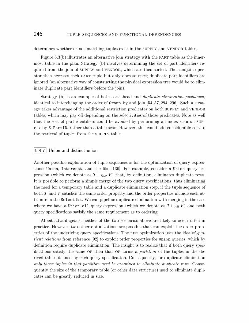
246 tuple sequences and functional dependencies
determines whether or not matching tuples exist in the supply and vendor tables.
Figure 5.3(b) illustrates an alternative join strategy with the part table as the inner-most table in the plan. Strategy (b) involves determining the set of part identifiers re-quired from the join of supply and vendor, which are then sorted. The semijoin oper-ator then accesses each part tuple but only does so once; duplicate part identifiers areignored (an alternative way of constructing the physical expression tree would be to elim-inate duplicate part identifiers before the join).
Strategy (b) is an example of both sort-ahead and duplicate elimination pushdown,identical to interchanging the order of Group by and join [54, 57, 294–296]. Such a strat-egy takes advantage of the additional restriction predicates on both supply and vendortables, which may pay off depending on the selectivities of those predicates. Note as wellthat the sort of part identifiers could be avoided by performing an index scan on sup-ply by S.PartID, rather than a table scan. However, this could add considerable cost tothe retrieval of tuples from the supply table.
5.4.7 Union and distinct union
Another possible exploitation of tuple sequences is for the optimization of query expres-sions: Union, Intersect, and the like [136]. For example, consider a Union query ex-pression (which we denote as T ∪Dist V ) that, by definition, eliminates duplicate rows.It is possible to perform a simple merge of the two query specifications, thus eliminatingthe need for a temporary table and a duplicate elimination step, if the tuple sequence ofboth T and V satisfies the same order property and the order properties include each at-tribute in the Select list. We can pipeline duplicate elimination with merging in the casewhere we have a Union all query expression (which we denote as T ∪All V ) and bothquery specifications satisfy the same requirement as to ordering.
Albeit advantageous, neither of the two scenarios above are likely to occur often inpractice. However, two other optimizations are possible that can exploit the order prop-erties of the underlying query specifications. The first optimization uses the idea of quo-tient relations from reference [92] to exploit order properties for Union queries, which bydefinition require duplicate elimination. The insight is to realize that if both query spec-ifications satisfy the same op then that op forms a partition of the tuples in the de-rived tables defined by each query specification. Consequently, for duplicate eliminationonly those tuples in that partition need be examined to eliminate duplicate rows. Conse-quently the size of the temporary table (or other data structure) used to eliminate dupli-cates can be greatly reduced in size.

5.5 related work in order optimization 247
The second optimization assists with the computation of Union all query expres-sions. Since duplicate tuples are not eliminated, the result can be computed simply as theconcatenation of the two inputs. However, consider a Union all query expression thatcontains an Order by clause. We can eliminate the subsequent sort step if the order prop-erty of both of its input query specifications can satisfy the interesting order specified inthe query—that is, we push down the Order by clause into the underlying query speci-fications, and then merely merge the inputs. Simmen et al. [261] consider the possibilityof sort-ahead only for spj queries, particularly for sort-merge joins.
5.4.8 Intersection and difference
Similar to Union expressions, we can exploit order properties in the computation of theset operations Intersect and Intersect all. As with Union, for Intersect query ex-pressions we can exploit the partitioning of the rows if each of the inputs to the distinctintersection operator satisfy the same op. For Intersect all, however, a simple mergeof the inputs is not sufficient to yield the correct result unless both query specificationssatisfy the same order property that contains each item in their respective Select lists.However, partitioning the tuples by their order property (in each input) can still yield astrategy that may be cheaper than sorting both inputs in their entirety. Similar process-ing can be performed for query expressions involving Except and Except all (the oper-ators distinct difference and difference, respectively).
5.5 Related work in order optimization
Commercial relational database systems, such as ibm’s db2 Universal Database, haveexploited sort order in indexed access methods for some time. To our knowledge, how-ever, Simmen, Shekita, and Malkemus [261, 262] appear to be the first researchers to dis-cuss the theory of order optimization in the literature. They also describe several aspectsof the implementation of this theory in db2. Much of the work presented in this chap-ter was developed independently of Simmen et al. One of our main contributions is toprove the sufficient and necessary conditions for propagating order properties through ajoin, a problem which Simmen et al. mention only in passing.
The basic theory of tuple sequences and several ideas about the relationship betweenfunctional dependencies and unique indexes is given by Abiteboul and Ginsburg [3]. Gins-berg and Hull [104] mention applications of sort set analysis (a class of order dependen-cies) to physical storage implementations in relational database systems, and allude to

248 tuple sequences and functional dependencies
the possibility of reducing the time spent on sorting during query processing by tak-ing advantage of the order of the tuples as they are stored on disk. They do not, how-ever, investigate the application of the theory to query processing and optimization. Sim-ilarly, some recent results by Ng [217] parallel both the work herein, and that of Simmenet al. Ng defines a sound and complete axiom system for ordered functional dependen-cies over an ordered relational model, using two similar but subtly different extensionsfor domains: pointwise orderings and lexicographical orderings. Ng’s model, however, isnot based on ansi sql and does not address the existence of null values, duplicate rows,or three-valued logic. Interestingly, the main application of his work appears to be nor-malized schema design for an ordered relational database; there is no mention of the use-fulness of order dependencies in query optimization. Dayal and Goodman [76] study treequery optimization in the context of the Multibase system but do not consider exploit-ing tuple sequences. In their timber system, Stonebraker and Kalash [268] consider se-quences of tuples as a possible storage mechanism to support text retrieval applicationsbut do not elaborate on optimization techniques that exploit timber’s storage model.
Another possible technique for combining order properties with the semantics of se-quences of tuples is to extend the notion of quotient relations [92], which offer a well-defined relational algebra that operates over partitions of relations that are equivalent forsome set of attributes X. In effect, these partitions are the ‘groups’ that result when per-forming a Group by over X on any arbitrary query. The extension required is to add anordering relationship between the groups of tuples.
5.6 Conclusions
In this chapter we formally described the necessary and sufficient conditions for aug-menting and reducing order properties, which included the specification of table and col-umn constraints and handled the three-valued logic of ansi sql. We also presented suf-ficient conditions for determining if the order properties satisfied by two tuple sequencescould be concatenated when performing inner or outer nested-loop and sort-merge joins.Part of this research brought together formalisms on tuple sequences [3] and prior workin query processing [92] that was absent in reference [261]. We also expanded the num-ber of types of ‘interesting orders’ that we can exploit in query processing: in addition tosort avoidance with joins, Distinct, and Group by, order properties are useful to:
• optimize query expressions with or without duplicate elimination,
• optimize simple queries containing Min() or Max() aggregate functions,
• optimize aggregate functions with duplicate elimination,

5.6 conclusions 249
• reduce the size of a cache for subquery memoization,
• cut the processing of an indexed search condition, and
• lower the cost of indexed retrieval by probing with a sorted set of secondary keys.
We believe there are several additional opportunities for exploiting order properties inquery optimization. One very promising area mentioned previously is in the optimizationof queries where the result set size is bounded, for example with the specification of Top nor Bottom n queries [42–44]. Exploiting this information is an active research area forvendors whose databases are used in olap applications. Sort order analysis is also usefulin environments where the user desires an access plan optimized for response time insteadof resource consumption.


6 Conclusions
Knowledge of functional dependencies, particularly key dependencies, is vital to the op-eration of a sophisticated query optimizer. All commercial database systems exploit func-tional dependencies in a variety of ways. However, we believe that most, if not all, of thequery optimizers in these implementations could be improved by expanding the set ofmaintained constraints to include lax functional dependencies, equivalence constraints,and null constraints. The fact that oracle8i [26] permits a database administrator toexplictly declare functional dependencies that hold in a given schema using oracle’sDimension objects is evidence that not only are dependencies useful for optimization—inthe case of reference [26], to permit the query optimizer to exploit the existence of materi-alized views—but that the existing tools and techniques for their analysis are insufficient.
Our primary goal in this thesis was to develop an algorithm to capture this arrayof dependency and constraint information for an arbitrary relational algebra expression.Our main contributions can be summarized as follows:
1. a formal definition of an extended relational model that includes real and virtualattributes, three-valued logic, and multiset semantics, and a set of algebraic oper-ators over that model that correspond to the major algebraic operators supportedby ansi sql, particularly outer joins;
2. definitions of lax functional dependencies and equivalence constraints that effec-tively model ansi sql’s unique constraints, true-interpreted predicates, and outerjoins;
3. a sound axiom system for a combined set of strict and lax functional dependenciesand equivalence constraints;
4. a formal characterization of the dependencies and constraints that hold in the resultof each algebraic operator, particularly the problematic operators left-, right-, andfull-outer join;
5. an extended fd-graph representation and an algorithm that correctly represents theset of valid dependencies and constraints that hold in the result of each operatorand that can be simply augmented to capture additional constraints;
251

252 conclusions
6. a suite of rewrite optimizations, formally proved, that exploit derived functionaldependencies to transform queries into semantically equivalent variants that mayoffer the opportunity to discover better access plans;
7. a set of theorems that describe the interaction of order properties and functionaldependencies, and examples of how exploiting these dependencies can lead to im-proved access plans, particularly by avoiding unnecessary sorts.
Our theoretical results provide a metaphorical channel through the ‘semantic reef’ ofthe optimization of outer joins. By characterizing the dependencies and equivalence con-straints that hold with outer joins, we permit a wider class of optimization techniquesto be applied to queries, views, or materialized views containing them. However, we be-lieve that additional work on outer join optimization is still necessary to ‘widen’ and‘deepen’ this channel. If we have learned anything through the development of this the-sis, it is that the optimization of outer join queries remains a considerable challenge, boththeoretically and in practice.
Some of the work contained herein has already been adopted into commercial databaseproducts, providing their optimizers with an expanded set of tools to optimize complexqueries. Two variants of the simplified fd-graph algorithms described in Chapter 4 havebeen implemented in Sybase sql Anywhere, where they are used to determine the correct-ness of subquery-to-join transformations, including those which require subsequent dupli-cate elimination, and Distinct elimination on spj queries, nested queries, and spj views.These algorithms have been extended to now support queries containing left outer joins,grouping, and aggregation, and now also utilize equivalence constraints derived from con-ditions in a Where clause. A significant result from their implementation is that a largerclass of join elimination optimizations are now possible, which usually has a direct af-fect on a query’s execution time. We believe that other commercial systems have utilizedthe results in Chapter 4 (actually the results published in our earlier paper [228]) to im-prove their query rewrite transformations. Moreover, Bhargava, Goel, and Iyer [34] basedtheir work on outer join optimization on the formalisms developed in that paper. In ad-dition, some of the work in Chapter 5, notably on the optimization of In-list predicates(see Example 36), has also been implemented in Sybase sql Anywhere.
6.1 Developing additional derived dependencies
While the dependency and constraint inference algorithms presented in Chapter 3 de-velop and maintain a comprehensive set of constraints, there are many ways in which thealgorithms can be improved to exploit additional information. For example:

6.1 developing additional derived dependencies 253
1. The current analysis ignores the possible existence of other forms of complex 3-valued logic predicates in ansi sql. For example, to simplify the algorithms andproofs, we intentionally ignored predicates of the form ‘P (x) is unknown’, whichoccur rarely in practice.
2. Note that only a limited set of lax dependencies are developed for the On conditionin a full outer join. Hence a subsequent null-intolerant restriction predicate thatcould convert the full outer join to a left- or right-outer join will be unable to exploitthe missing dependencies.
3. Corollary 2, which provides an alternative means to maintain an existing strict func-tional dependency f : X −→ Y from the null-supplying side of an outer join, is alsomerely a sufficient condition. One could utilize an existing null constraint X + Y
in the outer join’s null-supplying side to show that f continues to hold in the outerjoin’s result as a strict functional dependency.
4. Consider the left outer join Q = Sp−→ T where p contains the conjunctive, null-
intolerant condition S.X = T.Y. If X is a key of S then the strict functional depen-dency f : X −→ Y will always hold in the result, even though X �ω= Y (due to thepossible generation of an all-Null row) and, for the same reason, Y �−→ X.
5. Similarly, consider the left outer query Q as above, but where p consists of the sin-gle atomic condition S.X = 5. While this condition does not produce a lax or strictdependency, it does produce another form of constraint: for each tuple in the re-sult where S.X is not equal to 5, the value of each attribute in sch(T ) is Null. Infact, this is a generalization of a null constraint. Rather than a constraint betweentwo attributes X and Y , as per Definition 38 on page 95, we instead could writeP (X) + Y to reflect that if the predicate P on attribute(s) X evaluates to truethen attribute Y must be Null. This more generalized form of null constraint couldbe exploited during optimization in several ways. In the example above, such con-straints can used to determine the distribution of values for each result attributethat stems from sch(T ), which could lead to a more accurate cost estimate. A simi-lar situation exists with full outer joins. If Q = S
p←→ T and the On condition p con-tains the conjunct S.X = 5, then any tuple q0 in the result containing an S.X-valuethat is neither 5 nor Null contains the all-Null row of T .
6. As mentioned in Section 3.4.2, we could develop classes of scalar functions so thatif we have λ(X) in a Select list or predicate, and we can guarantee that the valuereturned from λ cannot be Null, then we can ‘push’ that restriction to make theinference that X also cannot be Null, forming the existence constraint x , λ(X)

254 conclusions
for each x ∈ X. There are likely other possible ways in which we can manufactureand exploit existence constraints with respect to inferring functional dependencies.
Moreover, improvements to the Restriction algorithm that would recognize strict orlax functional dependencies from a more varied Boolean expression could yield additionalopportunities for optimization improvements, as this predicate analysis could be utilizednot only for restriction but for the outer join operators as well36.
The changes required to extend the set of dependencies and/or constraints capturedin an fd-graph largely depend on whether or not the new information simply adds an-other instance of an existing constraint, or forms an altogether new class of constraint.For example, suppose that we wished to extend Cartesian product (Section 3.4.4) to ex-ploit the knowledge that one or both of its inputs consists of at most a single row. Con-sider the expression Q = S × T . Such a case would occur, for example, if either of theinput expressions, say eT , represented a grouped query that did not contain any group-ing attributes (AG = ∅). In this case, there is no need to construct a new tuple identifiervertex to represent the result of Q. Instead, we need only add strict functional dependen-cies from the vertex vk ∈ V R[GS ] that represents ι(S) to each of the vertices in V A[GT ].
On the other hand, capturing a new form of constraint will likely require additionalclasses of vertices and edges. Such an enhancement would involve:
1. proving that the new dependency or constraint would hold in the result of thatoperator over any instance of the database;
2. analyzing the other operators to determine if the new dependency would remainvalid in the result of each;
3. extending the data structures in the fd-graph to represent the constraint;
4. modifying the appropriate fd-graph algorithm(s) to capture the new constraint;
5. possibly modifying other algorithms in order to retain or remove this constraint asnecessary;
6. proving the correctness of each modified algorithm.
36 For example, David Toman has suggested modelling scalar functions and other complex pred-icates of n parameters by constructing a table with n + 1 columns of infinite domains, andrewriting the original query to include these ‘virtual’ tables by deriving the necessary joinpredicates from the set(s) of function parameters. In this manner the analysis of strict andlax dependencies due to functions can be reduced to the more straightforward analysis of con-junctive equality conditions.

6.2 exploiting uniqueness in nonrelational systems 255
6.2 Exploiting uniqueness in nonrelational systems
Our original motivation for determining how derived functional dependencies could beused in semantic query optimization was to find ways to expand the strategy space for op-timizing ansi sql queries—particularly nested queries and joins—against relational viewsof ims databases [131]. We believe these transformations are useful for any database modelthat uses pointers between objects. Pointer-based systems differ from traditional rela-tional systems in that the cost of processing a particular algebraic operator in a pointer-based database system can vary significantly from the cost of processing the same oper-ator in a ‘pure’ relational system.
As mentioned previously, several researchers [74, 101, 155, 157, 212, 230, 291] have stud-ied ways to rewrite nested queries as joins to avoid a nested-loops execution plan. Whenthe query is converted to a join, the optimizer is free to choose the most efficient joinstrategy while maintaining the semantics of the original query; the assumption is that anested-loops strategy is inefficient and seldom worth considering.
On the other hand, non-relational systems such as ims and various object-orienteddatabase systems are essentially navigational and queries against these data models in-herently use a nested-loops approach. In this section, we propose converting joins to sub-queries as a possible execution strategy in these systems. Our examples below illustratethat nested-loop processing remains an attractive execution strategy, under certain con-ditions, with a variety of database architectures.
6.2.1 IMS
Part of the cords multidatabase project at the University of Waterloo [15] aimed to findways to support ansi-standard sql queries against relational views of ims databases [170,171]. Essentially, the sql gateway optimizer attempted to translate an sql query into aniterative dl/i program consisting of nested loops of ims calls [133]. Queries that cannotbe directly translated by the data access layer—which executes the iterative program—require facilities of the post-processing layer that can perform more complex operationsnot directly supported by dl/i, such as sorting or aggregation, but at increased cost [170].Therefore, nested-loop strategies, which require only the gateway’s data access layer, mayoften be cheaper to execute.
Example 38
Consider the select-project-parent/child join query

256 conclusions
Select All V.*
From Vendor V, Supply S
Where S.VendorID = V.VendorID and S.PartID = :PARTNO
which lists all suppliers who have supplied a particular part, denoted by the host variable:PARTNO. This query can be handled exclusively by the data access layer by utilizing theapplication view in Figure A.4(a). A straightforward nested-loop join strategy is:
GU VENDOR;1717
while status = ‘ ’ do1718
GNP VSUPPLY (PartID = :PARTNO);1719
while status = ‘ ’ do1720
output VENDOR tuple;1721
GNP VSUPPLY (PartID = :PARTNO)1722
od ;1723
GN SUPPLIER1724
od1725
The subquery block satisfies conditions similar to those in Theorem 12, which in turndepends on being able to infer derived key dependencies, and therefore can exploit themechanisms detailed in Chapter 3. For this example, a necessary condition is that at mosta single instance (segment) of vsupply can join with each vendor. Therefore, we canrewrite this query as
Select All S.*
From Vendor V
Where Exists (Select *
From Supply S
Where V.VendorID = S.VendorID
and S.PartID = :PARTNO ).
This transformation simplifies the iterative method above, since the inner nested loopcan stop as soon as one qualifying vsupply segment is found:
GU VENDOR;1726
while status = ‘ ’ do1727
GNP VSUPPLY (PartID = :PARTNO);1728
if status = ‘ ’ then1729
output VENDOR tuple1730
fi ;1731
GN VENDOR1732
od1733

6.2 exploiting uniqueness in nonrelational systems 257
This version reduces the number of dl/i calls against the vsupply segment by half,since the second GNP call in the join strategy (line 1722) will always fail with a ‘GE’ (notfound) status code. A greater cost reduction may occur if the optimizer can convert ajoin that specifies non-key attributes in the join predicate to a nested query. For exam-ple, suppose the Supply table contained the attribute OEM-PartID, which in the ims im-plementation would likely be represented as a unique SRCH field in the vsupply segment.In the join strategy above, dl/i would have to scan all vsupply segments with the givenoem part number, instead of halting the search when the next segment’s key was greaterthan :PARTNO. The nested version halts the search immediately once dl/i finds a match.
6.2.2 Object-oriented systems
In some object-oriented database systems, physical object identifiers (oids) take the placeof foreign keys; both exodus and O2 take this approach [256]. However, oids differ frompointers in ims because each child object points to its parent (see Figure 6.1.) This pointerscheme does not effectively support select-project-join queries in which the selection pred-icate on the parent class (for example, vendor is more restrictive than the predicate ona subordinate class, because the most efficient way to process this type of join would re-quire pointers in the opposite direction [256, pp. 46].
Example 39
Consider the following join between vendor and supply in an object-oriented databasesystem (assume that the object-oriented system supports the use of path expressions, asin reference [301], in the sql variant used herein):
Select All V.*
From Supply S, Vendor V
Where V.VendorID Between ‘000AA000’ and ‘000AAB000’ and
V.S.SupplyCode = :SC
which lists all part vendors whose identifiers lie in the range ‘000AA000’ to ‘000AAB000’and whose supply code is equivalent to the input host variable :SC. A straightforwardnested-loop join strategy is:
retrieve SUPPLY;1734
while suppliers remaining do1735
if SUPPLY.SUPPLYCODE = :SC then1736
retrieve SUPPLY.VENDOR;1737
if SUPPLY.VENDOR.VendorID is between ‘000AA000’ and ‘000AAB000’ then1738
output VENDOR object1739
fi1740
fi ;1741

258 conclusions
PartIDDescriptionStatusQuantityPriceCostSupport
Part
VendorIDNameContactNameAddressBusPhoneResPhone
Vendor
Supplies
RatingSupplyCodeLagtime
Supply
ClassCodeDescriptionStatus
Part Class
EffectiveDateExpiryDateMinOrderUnitPriceQtyPrice
Quote
Contained in
offe
rs1+
Figure 6.1: Rumbaugh omt object-oriented data model for the parts-related classes. Weassume object identifiers (oids), implemented as physical pointers, replace foreign keysas the relationship mechanism between objects. Each class has a surrogate key attributeto aid in object identification.
retrieve next SUPPLY1742
od1743
This strategy may be inefficient because many vendor objects may be referenced, onlyto find that their identifier is not in the specified range—this would be the case, for in-stance, if many vendors supplied parts with a supply code of :SC. From Theorem 12,however, we can rewrite the query in Example 39 as the nested query
Select All V.*
From Vendor V
Where V.VendorID between‘000AA000’ and ‘000AAB000’ and
Exists (Select *
From Supply S
Where S.SupplyCode = :SC ).
Assuming we have an index on supply by supply code, and an index on vendor byvendor identifier, then a more efficient strategy may be as follows:
retrieve VENDOR (VendorID between‘000AA000’ and ‘000AAB000’);1744

6.3 other applications and open problems 259
while vendors remaining do1745
retrieve SUPPLY (SupplyCode = :SC and SUPPLY.VENDOR.OID = VENDOR.OID);1746
if found then1747
output VENDOR object1748
fi ;1749
retrieve next VENDOR (VendorID between‘000AA000’ and ‘000AAB000’);1750
od1751
depending on the objects’ selectivity. The idea is to restrict the search of the supply classto only those instances that correspond to a vendor instance whose vendor identifiermatches the range predicate.
6.3 Other applications and open problems
The formalisms we developed in Chapter 2, in particular our definitions of strict andlax functional dependencies, equivalence constraints, and null constraints, and the for-malisms for order properties and their interaction with these constraints, allow for thesystematic study of other, closely related optimization problems. For example, the set ofalgebraic operators described in this thesis are merely the ‘basic’ ones needed to mirror areasonably large class of query expressions in ansi sql. However, database systems im-plement a wider variety of executable algebraic operators: inner semijoin, left-outer semi-join, full-outer semijoin, exists join [29, 74, 146], variant forms of ‘generalized outer join’[30, 31, 34, 94, 95, 98], and so on; Graefe’s recent survey [107] provides a useful overview.Each of these operators requires careful analysis to determine the sets of dependenciesand constraints that hold in their result.
The theoretical results contained herein can be extended in a variety of ways. We lim-ited our modelling of constraints to those ansi sql column and table constraints thatcould be specified in a Check clause; we did not attempt to exploit other forms of con-straints, such as multivalued dependencies, referential integrity constraints (inclusion de-pendencies), and the more general form of sql table constraints termed assertions. Wemade no attempt to prove the completeness of the inference axioms for strict and lax de-pendencies, defined in Chapter 2, and strict and lax equivalence constraints, defined inChapter 3. We have also not analyzed the algorithms’ efficiency, nor have we constructeda prototype to experiment with various implementations to find an efficient one (see Sec-tion 3.8 for some additional remarks).
We believe these results have wide applicability to query processing and optimiza-tion. As a first example, consider the optimization of universally-quantified subqueries(see Section 2.3.1.2). Most query optimizers do not optimize these types of queries in a

260 conclusions
sophisticated fashion [109]; part of the reason is the existence of true-interpreted corre-lation predicates, which are difficult to exploit for index processing. However, modellinga query’s equivalence constraints with an fd-graph may permit such a predicate to betransformed into a semantically equivalent, false-interpreted one, permitting the correla-tion predicate to be used as a ‘standard’ matching predicate for indexed retrieval.
Other applications of our work on derived dependencies include:
1. exploiting derived dependencies during the optimization of queries over material-ized views [26, 52, 53, 57, 174, 297];
2. using dependencies, equivalence constraints, and null constraints for materializedview maintenance, particularly for those views containing one or more outer joins[118, 119];
3. extending the work of Medeiros and Tompa [198] on view update policies to supportthe update of views over ansi sql tables, not simply relations, and to verify thatthe constraints (unique indexes, unique constraints, Check constraints, assertions,and so on) defined on them cannot be violated.

A Example schema
Our example database scheme contains employee, part, and supplier information for ahypothetical mechanical parts distribution firm, with divisions located in Chicago, NewYork, and Toronto. The firm’s inventory consists of a wide variety of parts, from fastenersto widgets, manufactured by a variety of suppliers throughout North America. Figure A.1contains an entity-relationship diagram that models the schema.
A.1 Relational schema
Parts. The firm’s parts inventory is represented by several base tables which contain infor-mation about each part, its supplier(s), its status, and its cost. Parts are organized intoclasses, which serves to classify parts into groups for easier management and tracking.
Create Table Class (
ClassCode char(2) not null,
Description char(20) not null,
Status char(1)
Primary Key (ClassCode));
Create Table Part (
PartID char(8) not null,
Description char(30) not null,
Status char(8),
Qty numeric(7),
Price numeric(7,2) not null,
Cost numeric(7,2) not null,
Support char(2) not null,
ClassCode char(2) not null
Primary Key (PartID)
Foreign Key (ClassCode) references Class
Check (Qty �= 0 Or Status = ‘InStock’)
Check (Price ≥ Cost));
261

262 example schema
Vendors. Each part may be supplied by more than one supplier (termed a vendor), andthe supply table contains a row for each part-vendor relationship. Vendors are ‘ranked’for each part they supply.
Create Table Supply (
VendorID char(8) not null,
PartID char(8) not null,
Rating char(1),
SupplyCode char(4),
Lagtime numeric(7) not null
Primary Key (PartID, VendorID)
Foreign Key (PartID) references Part
Foreign Key (VendorID) references Vendor
Check (Rating in( ‘A’, ‘B’, ‘C’) ));
It is assumed that periodically a part vendor will respond to a quotation request andoffer a specific part for a certain price. The quote table represents this intersection datadetailing the quote of a part’s price by that particular vendor for a certain date range.
Create Table Quote (
QuoteID char(7) not null,
EffectiveDate date not null,
ExpiryDate date not null,
MinOrder numeric(5) not null,
UnitPrice numeric(7,2) not null,
QtyPrice numeric(7,2) not null,
PartID char(8) not null,
VendorID char(8) not null
Primary Key (PartID, VendorID, QuoteID)
Foreign Key (PartID, VendorID) references Supply);
Finally, part vendors and their contacts are defined by the vendor table. The datamodel assumes that vendor names are unique.
Create Table Vendor (
VendorID char(8) not null,
Name char(40),
ContactName char(30),
Address char(40),
BusPhone char(10),
ResPhone char(10)
Primary Key (VendorID)
Unique (Name));
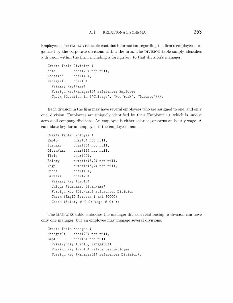
a.1 relational schema 263
Employees. The employee table contains information regarding the firm’s employees, or-ganized by the corporate divisions within the firm. The division table simply identifiesa division within the firm, including a foreign key to that division’s manager.
Create Table Division (
Name char(20) not null,
Location char(40),
ManagerID char(5)
Primary Key(Name)
Foreign Key(ManagerID) references Employee
Check (Location in (‘Chicago’, ‘New York’, ‘Toronto’)));
Each division in the firm may have several employees who are assigned to one, and onlyone, division. Employees are uniquely identified by their Employee id, which is uniqueacross all company divisions. An employee is either salaried, or earns an hourly wage. Acandidate key for an employee is the employee’s name.
Create Table Employee (
EmpID char(5) not null,
Surname char(20) not null,
GivenName char(15) not null,
Title char(20),
Salary numeric(6,2) not null,
Wage numeric(6,2) not null,
Phone char(10),
DivName char(20)
Primary Key (EmpID)
Unique (Surname, GivenName)
Foreign Key (DivName) references Division
Check (EmpID Between 1 and 30000)
Check (Salary �= 0 Or Wage �= 0) );
The manages table embodies the manager-division relationship; a division can haveonly one manager, but an employee may manage several divisions.
Create Table Manages (
ManagerOf char(20) not null,
EmpID char(5) not null
Primary Key (EmpID, ManagerOf)
Foreign Key (EmpID) references Employee
Foreign Key (ManagerOf) references Division);

264 example schema
Finally, each employee is responsible for the inventory of one or more parts, whichare identified by a unique part identifier. Each part may be managed by more than oneemployee.
Create Table ResponsibleFor (
PartID char(8) not null,
EmpID char(5) not null
Primary Key (PartID, EmpID)
Foreign Key (EmpID) references Employee
Foreign Key (PartID) references Part);
A.2 IMS schema
ims, jointly developed by ibm Corporation and Rockwell International for the Apollospace program in the 1960s, permits application programs to navigate through a set ofdatabase records stored as a hierarchy. The hierarchy defines one-to-many relationshipsbetween segments (or, more properly, segment types), with a root segment at the top ofeach ‘tree’. Each database record consists of a root segment occurrence and all occur-rences of its dependent segments. Each root segment type in a hidam, hdam, or hisamdatabase must have a sequence field that may either be unique or non-unique. The se-quence field is used by ims to locate a specific root segment occurrence: with hdam ahashing technique is used, while with hidam and hisam databases an index is used to re-trieve root segment occurrences by their sequence field. With dependent segments the se-quence field is optional. If one is defined, ims stores the dependent segment occurrencesin ascending order of the sequence field. If a dependent segment type lacks a sequencefield, then ims will insert new segment occurrences at an arbitrary point under that seg-ment type’s ancestor in the hierarchy, the precise position determined by the applicationprogram at execution.
If the sequence field of a particular segment type is unique, and each of its physi-cal ancestors in the database record also have unique sequence fields, then each segmentoccurrence can be uniquely identified by the concatenation its sequence field and the se-quence fields of each segment occurrence in its hierarchic path. In ims terminology thisis termed the segment’s fully concatenated key.
A physical ims database may have up to 15 levels (the parts database illustrated inFigure A.3 has four) and up to 255 segment types. The database administrator defines adatabase with a database description, commonly referred to as a dbd.
Application programs navigate through the database hierarchy, retrieving one seg-ment at a time, using the ims application program interface Data Language/One (dl/i).

a.2 ims schema 265
The application view of a physical or logical ims database is described in a Program Con-trol Block, or pcb (see Figure A.4). The segment hierarchy defined in a pcb may be com-posed of a physical hierarchy, meaning that all the segments in the view are from thesame physical ims database, or they may be composed of a logical hierarchy, which uti-lizes logical child/logical parent relationships to form a hierarchical view of segments fromdifferent physical databases. Note that a database level cannot be ‘missing’ from an ap-plication view described by an ims pcb.
Since dl/i is such a low-level api (see Table A.1) the application programmer is re-sponsible for optimizing how the application retrieves its required information, includ-ing the use of any indexes that may exist; hence index usage in ims is not transparentto the application. Furthermore, the programmer must be aware of the effects of differ-ent ims access methods. For example, an hdam and a hidam database with identicalschemas can return different results to an application program because of hdam’s hashedaccess to root segments.
dl/i Call Purpose
GU Get Unique: retrieve the first segment occurrence inthe database that satisfies the ssas
GN Get Next: retrieve the next segment from the currentposition in hierarchical order
GNP Get Next Within Parent: retrieve the next dependentsegment occurrence under the present ancestor
Table A.1: dl/i calls. Each retrieval call has a ‘hold’ option (GHU, GHN, and GHNP, respec-tively) that positions a program on a particular segment occurrence and locks it, prior toits replacement or deletion.
A complete description of ims databases and application programming are beyond thescope of this thesis. More details regarding the dl/i interface can be found in references[36, 133, 276].
A.2.1 IMS physical databases
Figures A.2 and A.3 depict the three example databases used to implement the ims ver-sion of the data model described in Figure A.1. In the employee physical database, em-ployees are modelled as dependent segments under the division that employs them. re-

266 example schema
spbfor and manages are logical child segments that respectively implement the many-to-many relationship employees and the parts they are responsible for, and the one-to-many relationship between divisions and managers. With many-to-many relationships,logical child segments are often paired, meaning that while two different segment typesare used to model the many-to-many relationship (one in each physical hierarchy) onlyone segment type is actually stored in the database. In this way, ims ensures a consis-tent database when an application program inserts, updates, deletes a relationship seg-ment. Table A.2 cross-references each logical child segment in the example schema withits pair. In contrast, manages is a one-to-many relationship, embodying the constraintthat each division can have only one manager. Hence manages is not logically pairedwith any other segment.
A.2.2 Mapping segments to a relational view
Background information regarding the mapping of an ims schema to a relational view canbe found in references [170] and [172], but we briefly state the essentials here; a compre-hensive discussion is beyond the scope of this thesis. Each ims segment type is mapped toa virtual table that contains corresponding attributes. Parent-child relationships are mod-eled as foreign keys; the fully concatenated key of each dependent segment type is used asthe key of its virtual table in the relational view. In this thesis we assume that each seg-ment type has a unique sequence field, which can serve as a key. In practice, most seg-ment types in ims databases have unique sequence fields, enabling faster retrieval andavoiding the situation where the position of a segment in the database has some intrin-sic meaning to application programs. Key attributes inherited from parent segment typesare termed virtual attributes. For example, DivName is a virtual column, derived fromthe division segment, in the relational view of the employee segment.
Logical relationships provide a particular challenge for query optimization. For exam-ple, the paired bi-directional logical child segments psupply and vsupply embody themany-to-many relationship between parts and vendors. There are two logical child seg-ment types to permit navigation in both directions, though the contents of a paired psup-ply and vsupply are identical but for their logical parent pointers. In the relational view,one table is created (supply) to represent this data; however, the gateway’s optimizermust choose the direction, and therefore the logical child segment, in which to traversethe relationship to retrieve a query’s result using the fewest resources.
As an aside, we note that there do exist several commercial products, notably In-gres’ gateway products [135] (now offered by Computer Associates), ibm’s DataJoiner,and Oracle’s sql Connect to ims [222] that all provide relational access, via sql queries,to ims databases. All of these commercial products fail to offer a comprehensive solution

a.2 ims schema 267
Segment Paired Pairing Logical
with method parent
respbfor emprespb virtual part
vsupply psupply physical part
emprespb respbfor virtual employee
manages n/a unidirectional division
psupply vsupply physical vendor
Table A.2: Logical relationships in the ims schema
to both the problem of mapping an ims database to a relational view, and to the prob-lem of transforming update operations done on the view to physical database operations.
In the parts physical ims database, the part segment is a child of the class seg-ment, which is the root segment (see Figure A.3). In turn, emprespb and psupply areboth dependent segments of part, and are thus termed siblings. Using analogous termi-nology, twin segments are multiple occurrences of a segment type under the same parentsegment occurrence.
Figure A.4 diagrams two application views of the Vendor database. Figure (a) illus-trates a straightforward view of the physical Vendor database consisting of the two phys-ical segments vendor and vsupply. The second pcb in Figure (b) illustrates the af-fect logical relationships has on the structure of the hierarchical view seen by the appli-cation program. In this example, the concatenated logical parent consisting of vsupplyand part permits the application to view a hierarchy combining the Vendor databasewith components of the Part database. Moreover, note how the class segment, the rootof the physical Parts database, is now described in the hierarchy as a child of the con-catenated logical parent segment vsupply/part.

268 example schema
Division
Employee
works in
Manages
M
1
1
M
Parts
Responsiblefor
Classcategory
M
N
M
1
QuoteVendor
Supply
M
M M
Figure A.1: e/r diagram of the manufacturing schema. Entities and relationships thatbegin with capital letters are represented by base tables.

a.2 ims schema 269
manages respbfor
employee
division
Figure A.2: Employee ims database. Solid boxes denote physical segments; dashedboxes denote logical, or pointer, segments. The database organization is hidam [132] withparent-child/twin pointers; root segments are key-sequenced through the database’s pri-mary index.
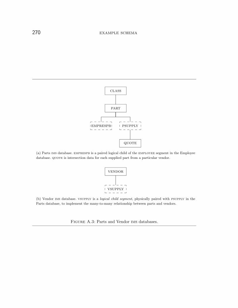
270 example schema
emprespb
quote
psupply
part
class
(a) Parts ims database. emprespb is a paired logical child of the employee segment in the Employee
database. quote is intersection data for each supplied part from a particular vendor.
vsupply
vendor
(b) Vendor ims database. vsupply is a logical child segment, physically paired with psupply in the
Parts database, to implement the many-to-many relationship between parts and vendors.
Figure A.3: Parts and Vendor ims databases.

a.2 ims schema 271
vsupply
vendor
(a) Application view (pcb) of the physical Vendor database.
class
vsupply part
vendor
(b) Application view (pcb) of a logical Vendor database using the concatenated logical child segment
consisting of vsupply and part.
Figure A.4: Two application views of the Vendor ims database.


B Trademarks
The following acronyms and abbreviations used in this thesis are trademarks or service-marks in Canada, the United States and/or other countries:
• ibm, db2, db2/mvs, ims/esa, ims/tm, dl/1, starburst, DataJoiner, System r,vsam, and mvs/esa are trademarks of International Business Machines Corpora-tion;
• ingres and quel are trademarks of Computer Associates;
• oracle, oracle8i, and sql*connect are trademarks of Oracle Corporation;
• sybase, sybase iq, sql Anywhere Studio, Adaptive Server Anywhere, and Adap-tive Server Enterprise are trademarks of Sybase, Inc.
Other product names contained herein may be trademarks or servicemarks of their re-spective companies.
273


Bibliography
[1] Serge Abiteboul and Oliver M. Duschka. Complexity of answering queries usingmaterialized views. In Proceedings, acm sigact-sigmod-sigart Symposium onPrinciples of Database Systems, pages 254–263, Seattle, Washington, June 1998.Association for Computing Machinery.
[2] Serge Abiteboul and Seymour Ginsburg. Tuple sequences and indexes. In Proceed-ings, 11th Colloquium on Automata, Languages, and Programming (icalp), pages41–50, Antwerp, Belgium, July 1984. Springer-Verlag.
[3] Serge Abiteboul and Seymour Ginsburg. Tuple sequences and lexicographic in-dexes. Journal of the acm, 33(3):409–422, July 1986.
[4] Serge Abiteboul, Richard Hull, and Victor Vianu. Foundations of Databases. Addi-son-Wesley, Reading, Massachusetts, 1995.
[5] M[ichel] Adiba. Derived relations: A unified mechanism for views, snapshots anddistributed data. In Proceedings of the 7th International Conference on Very LargeData Bases, pages 293–305, Cannes, France, September 1981. ieee Computer So-ciety Press.
[6] Michel E. Adiba and Bruce G. Lindsay. Database snapshots. In Proceedings of the6th International Conference on Very Large Data Bases, pages 86–91, Montreal,Quebec, October 1980. ieee Computer Society Press.
[7] A. V. Aho, C. Beeri, and J. D. Ullman. The theory of joins in relational databases.acm Transactions on Database Systems, 4(3):297–314, September 1979.
[8] A. V. Aho, Y. Sagiv, and J. D. Ullman. Equivalences among relational expressions.siam Journal on Computing, 8(2):218–246, May 1979.
[9] J[amal] R. Alsabbagh and V[ijay] V. Raghavan. A framework for multiple-queryoptimization. In Proceedings, Second International Workshop on Research Issuesin Data Engineering: Transaction and Query Processing, pages 157–162, Tempe,Arizona, February 1992. ieee Computer Society Press.
275

276 bibliography
[10] Jamal R. Alsabbagh and Vijay V. Raghavan. Analysis of common subexpressionexploitation models in multiple-query processing. In Proceedings, Tenth ieee Inter-national Conference on Data Engineering, pages 488–497, Houston, Texas, Febru-ary 1994. ieee Computer Society Press.
[11] Gennady Antoshenkov. Dynamic query optimization in rdb/vms. In Proceedings,Ninth ieee International Conference on Data Engineering, pages 538–547. ieeeComputer Society Press, April 1993.
[12] Gennady Antoshenkov. Dynamic optimization of index scans restricted by booleans.In Proceedings, Twelfth ieee International Conference on Data Engineering, pages430–440, New Orleans, Louisiana, February 1996. ieee Computer Society Press.
[13] W. W. Armstrong. Dependency structures of database relationships. In Proceedingsof the ifip Congress, pages 580–583, Stockholm, Sweden, August 1974. North-Hol-land.
[14] W. W. Armstrong and C[laude] Delobel. Decompositions and functional dependen-cies in relations. acm Transactions on Database Systems, 5(4):404–430, December1980.
[15] G[opi] K. Attaluri, D[exter] P. Bradshaw, N[eil] Coburn, P[er-Ake] Larson, P[atrick]Martin, A[vi] Silberschatz, J[acob] Slonim, and Q[iang] Zhu. The cords multi-database project. ibm Systems Journal, 34(1):39–62, 1995.
[16] Paolo Atzeni and Valeria De Antonellis. Relational Database Theory. Ben-jamin/Cummings, Redwood City, California, 1993.
[17] Paolo Atzeni and Nicola M. Morfuni. Functional dependencies in relations withnull values. Information Processing Letters, 18:233–238, 1984.
[18] Paolo Atzeni and Nicola M. Morfuni. Functional dependencies and constraints onnull values in database relations. Information and Control, 70(1):1–31, 1986.
[19] Giorgio Ausiello, Alessandro D’Atri, and Domenico Sacca. Graph algorithms forfunctional dependency manipulation. Journal of the acm, 30(4):752–766, October1983.
[20] G[iorgio] Ausiello, A[lessandro] D’Atri, and D[omenico] Sacca. Minimal represen-tation of directed hypergraphs. siam Journal on Computing, 15(2):418–431, May1986.

bibliography 277
[21] Giorgio Ausiello, Umberto Nanni, and Giuseppe F. Italiano. Dynamic maintenanceof directed hypergraphs. Theoretical Computer Science, 72(2–3):97–117, 1990.
[22] Catriel Beeri and Philip A. Bernstein. Computational problems related to the de-sign of normal form relation schemas. acm Transactions on Database Systems,4(1):30–59, March 1979.
[23] Catriel Beeri, Ronald Fagin, and John H. Howard. A complete axiomatization forfunctional and multivalued dependencies in database relations. In acm sigmodInternational Conference on Management of Data, pages 47–61, Toronto, Ontario,August 1977.
[24] Catriel Beeri and P[eter] Honeyman. Preserving functional dependencies. siamJournal on Computing, 10(3):647–656, August 1981.
[25] D. A. Bell, D. H. O. Ling, and S. I. McClean. Pragmatic estimation of join sizes andattribute correlations. In Proceedings, Fifth ieee International Conference on DataEngineering, pages 76–84, Los Angeles, California, February 1989. ieee ComputerSociety Press.
[26] Randall G. Bello, Karl Dias, Alan Downing, James Feenan, et al. Materialized viewsin oracle. In Proceedings of the 24th International Conference on Very Large DataBases, pages 659–664, New York, New York, August 1998. Morgan-Kaufmann.
[27] Kristin Bennet, Michael C. Ferris, and Yannis E. Ioannidis. A genetic algorithmfor database query optimization. In Proceedings of the 4th International Confer-ence on Genetic Algorithms, pages 400–407, San Diego, California, 1991. Morgan-Kaufmann.
[28] Philip A. Bernstein. Synthesizing third normal form relations from functional de-pendencies. acm Transactions on Database Systems, 1(4):277–298, December 1976.
[29] Philip A. Bernstein and Dah-Ming W. Chiu. Using semi-joins to solve relationalqueries. Journal of the acm, 28(1):25–40, January 1981.
[30] Gautam Bhargava, Piyush Goel, and Bala[krishna] Iyer. Reordering of complexqueries involving joins and outer joins. Research Report tr-03.567, ibm Corpora-tion, Santa Teresa Laboratory, San Jose, California, July 1994.
[31] Gautam Bhargava, Piyush Goel, and Bala[krishna] Iyer. Hypergraph based re-orderings of outer join queries with complex predicates. In acm sigmod Interna-tional Conference on Management of Data, pages 304–315, San Jose, California,May 1995.
278 bibliography
[32] Gautam Bhargava, Piyush Goel, and Bala[krishna] Iyer. No regression algorithmfor the enumeration of projections in sql queries with joins and outer joins. InProceedings of the 1995 cas Conference, pages 87–99, Toronto, Ontario, November1995. ibm Canada Laboratory Centre for Advanced Studies.
[33] Gautam Bhargava, Piyush Goel, and Bala[krishna] Iyer. Simplification of outerjoins. In Proceedings of the 1995 cas Conference, pages 63–75, Toronto, Ontario,November 1995. ibm Canada Laboratory Centre for Advanced Studies.
[34] Gautam Bhargava, Piyush Goel, and Bala[krishna] Iyer. Efficient processing of outerjoins and aggregate functions. In Proceedings, Twelfth ieee International Confer-ence on Data Engineering, pages 441–449, New Orleans, Louisiana, February 1996.ieee Computer Society Press.
[35] Joachim Biskup. A formal approach to null values in database relations. In HerveGallaire, Jack Minker, and Jean Nicolas, editors, Advances in Database Theory, vol-ume 1, pages 299–341. Plenum Press, New York, New York, 1981.
[36] Dines Bjørner and Hans Henrik Løvengreen. Formalization of database systems—and a formal definition of ims. In Proceedings of the 8th International Conferenceon Very Large Data Bases, pages 334–347, Mexico City, Mexico, September 1982.vldb Endowment.
[37] Jose A. Blakeley, Neil Coburn, and Per-Ake Larson. Updating derived relations:Detecting irrelevant and autonomously computable updates. acm Transactions onDatabase Systems, 14(3):369–400, September 1989.
[38] Jose A. Blakeley and Hector Hernandez. Multiple-query optimization for materi-alized view maintenance. Technical Report 267, Indiana University, Bloomington,Indiana, January 1989.
[39] Jose A. Blakeley, Per-Ake Larson, and F. W. Tompa. Efficiently updating materi-alized views. In acm sigmod International Conference on Management of Data,pages 61–71, Washington, D.C., May 1986.
[40] Jose A. Blakeley and Nancy L. Martin. Join index, materialized view, and hybrid-hash join: A performance analysis. In Proceedings, Sixth ieee International Confer-ence on Data Engineering, pages 256–263, Los Angeles, California, February 1990.
[41] Kjell Bratbergsengen. Hashing functions and relational algebra operations. In Pro-ceedings of the 10th International Conference on Very Large Data Bases, pages323–333, Singapore, August 1984. vldb Endowment.

bibliography 279
[42] Michael J. Carey and Donald Kossmann. On saying “Enough already!” in sql.In acm sigmod International Conference on Management of Data, pages 219–230,Tucson, Arizona, May 1997. Association for Computing Machinery.
[43] Michael J. Carey and Donald Kossmann. Processing top n and bottom n queries.ieee Data Engineering Bulletin, 20(3):12–19, September 1997.
[44] Michael J. Carey and Donald Kossmann. Reducing the braking distance of an sqlquery engine. In Proceedings of the 24th International Conference on Very LargeData Bases, pages 158–169, New York, New York, August 1998. Morgan-Kaufmann.
[45] Marco A. Casanova, Ronald Fagin, and Christos H. Papadimitriou. Inclusion de-pendencies and their interaction with functional dependencies. In Proceedings, acmsigact-sigmod-sigart Symposium on Principles of Database Systems, pages 29–59, Los Angeles, California, March 1982. Association for Computing Machinery.
[46] Marco A. Casanova, Ronald Fagin, and Christos H. Papadimitriou. Inclusion de-pendencies and their interaction with functional dependencies. Journal of Com-puter and System Sciences, 28(1):29–59, 1984.
[47] Stefano Ceri and Georg Gottlob. Translating sql into relational algebra: Optimiza-tion, semantics, and equivalence of sql queries. ieee Transactions on Software En-gineering, 11(4):324–345, April 1985.
[48] Stefano Ceri and Jennifer Widom. Deriving production rules for incremental viewmaintenance. In Proceedings of the 17th International Conference on Very LargeData Bases, pages 577–589, Barcelona, Spain, September 1991. Morgan Kaufmann.
[49] U[pen] S. Chakravarthy, John Grant, and Jack Minker. Foundations of semanticquery optimization for deductive databases. In Jack Minker, editor, Foundations ofDeductive Databases and Logic Programming, pages 243–273. Morgan Kaufmann,Los Altos, California, 1987.
[50] Upen S. Chakravarthy, John Grant, and Jack Minker. Logic-based approach to se-mantic query optimization. acm Transactions on Database Systems, 15(2):162–207,June 1990.
[51] Surajit Chaudhuri. An overview of query optimization in relational systems. In Pro-ceedings, acm sigact-sigmod-sigart Symposium on Principles of Database Sys-tems, pages 34–43, Seattle, Washington, June 1998. Association for Computing Ma-chinery.

280 bibliography
[52] Surajit Chaudhuri, Ravi Krishnamurthy, Spyros Potamianos, and Kyuseok Shim.Optimizing queries with materialized views. Technical Report hpl-dtd-94-16, hpResearch Laboratories, Palo Alto, California, February 1994. 25 pages.
[53] Surajit Chaudhuri, Ravi Krishnamurthy, Spyros Potamianos, and Kyuseok Shim.Optimizing queries with materialized views. In Proceedings, Eleventh ieee Inter-national Conference on Data Engineering, pages 190–200, Taipei, Taiwan, March1995. ieee Computer Society Press.
[54] Surajit Chaudhuri and Kyuseok Shim. Including group-by in query optimization. InProceedings of the 20th International Conference on Very Large Data Bases, pages354–366, Santiago, Chile, September 1994. Morgan Kaufmann.
[55] Surajit Chaudhuri and Kyuseok Shim. An overview of cost-based optimizationof queries with aggregates. ieee Data Engineering Bulletin, 18(3):3–9, September1995.
[56] Surajit Chaudhuri and Kyuseok Shim. Optimization of queries with user-definedpredicates. In Proceedings of the 22nd International Conference on Very Large DataBases, pages 87–98, Bombay, India, September 1996. Morgan Kaufmann.
[57] Surajit Chaudhuri and Kyuseok Shim. Optimizing queries with aggregate views. InP. Apers, M. Bouzeghoub, and G[eorges] Gardarin, editors, Advances in DatabaseTechnology—edbt’96 (Proceedings of the 5th International Conference on Extend-ing Database Technology), pages 167–182, Avignon, France, March 1996. Spring-er-Verlag.
[58] Surajit Chaudhuri and Moshe Y. Vardi. Optimization of real conjunctive queries.In Proceedings, acm sigact-sigmod-sigart Symposium on Principles of DatabaseSystems, pages 59–70, Washington, D. C., May 1993. Association for ComputingMachinery.
[59] Mitch Cherniack and Stan Zdonik. Inferring function semantics to optimize queries.In Proceedings of the 24th International Conference on Very Large Data Bases,pages 239–250, New York, New York, August 1998. Morgan-Kaufmann.
[60] Stavros Christodoulakis. Estimating record selectivities. Information Systems,8(2):105–115, 1983.
[61] Stavros Christodoulakis. Estimating block selectivities. Information Systems,9(1):69–79, 1984.

bibliography 281
[62] Stavros Christodoulakis. Implications of certain assumptions in database perfor-mance evaluation. acm Transactions on Database Systems, 9(2):163–186, 1984.
[63] Stavros Christodoulakis. On the estimation and use of selectivities in database per-formance evaluation. Technical Report cs–89–24, University of Waterloo, Water-loo, Ontario, Canada, June 1989.
[64] Sophie Cluet and Guido Moerkotte. On the complexity of generating optimal left-deep processing trees with cross products. In Proceedings of the Fifth InternationalConference on Database Theory—icdt’95, pages 54–67, Prague, Czech Republic,January 1995. Springer-Verlag.
[65] E. F. Codd. A relational model of data for large shared data banks. Communica-tions of the acm, 13(6):377–387, June 1970.
[66] E. F. Codd. Extending the database relational model to capture more meaning.acm Transactions on Database Systems, 4(4):397–434, December 1979.
[67] Latha S. Colby, Timothy Griffin, Leonid Libkin, Inderpal Singh Mumick, andHoward Trickey. Algorithms for deferred view maintenance. In acm sigmod In-ternational Conference on Management of Data, pages 469–480, Montreal, Quebec,June 1996. Association for Computing Machinery.
[68] Latha S. Colby, Akira Kawaguchi, Daniel F. Lieuwen, Inderpal Singh Mumick, andKenneth A. Ross. Supporting multiple view maintenance policies. In acm sig-mod International Conference on Management of Data, pages 405–416, Tucson,Arizona, May 1997. Association for Computing Machinery.
[69] Peter Corrigan and Mark Gurry. oracle Performance Tuning. O’Reilly & Asso-ciates, Sebastopol, California, 1993.
[70] Hugh Darwen. The role of functional dependence in query decomposition. In Rela-tional Database Writings 1989–1991, chapter 10, pages 133–154. Addison-Wesley,Reading, Massachusetts, 1992.
[71] C. J. Date. An Introduction to Database Systems, volume 1. Addison-Wesley, Read-ing, Massachusetts, fifth edition, 1990.
[72] C. J. Date and Hugh Darwen. A Guide to the sql Standard. Addison-Wesley, Read-ing, Massachusetts, fourth edition, 1997.
[73] Umeshwar Dayal. Query processing in a multidatabase system. In Kim et al. [159],pages 81–108.

282 bibliography
[74] Umeshwar Dayal. Of nests and trees: A unified approach to processing queries thatcontain nested subqueries, aggregates, and quantifiers. In Proceedings of the 13thInternational Conference on Very Large Data Bases, pages 197–208, Brighton, Eng-land, August 1987. Morgan Kaufmann.
[75] Umeshwar Dayal and Philip A. Bernstein. On the correct translation of updateoperations on relational views. acm Transactions on Database Systems, 8(3):381–416, September 1982.
[76] Umeshwar Dayal and Nathan Goodman. Query optimization for codasyl databasesystems. In acm sigmod International Conference on Management of Data, pages138–150, Orlando, Florida, June 1982.
[77] Janos Demetrovics, Leonid Libkin, and Ilya B. Muchnik. Functional dependenciesin relational databases: A lattice point of view. Discrete Applied Mathematices,40(2):155–185, December 1992.
[78] Jim Diederich. Minimal covers revisited: Correct and efficient algorithms. acm sig-mod Record, 20(1):12–13, March 1991.
[79] Jim Diederich and Jack Milton. New methods and algorithms for database normal-ization. acm Transactions on Database Systems, 13(3):339–365, September 1988.
[80] Martin Dietzfelbinger, Anna R. Karlin, Kurt Mehlhorn, Friedhelm Meyer auf derHeide, Hans Rohnert, and Robert E. Tarjan. Dynamic perfect hashing: Upper andlower bounds. siam Journal on Computing, 23(4):738–761, August 1994.
[81] Ramez Elmasri and Shamkant B. Navathe. Fundamentals of Database Systems.Benjamin/Cummings, Redwood City, California, 2nd edition, 1995.
[82] Raymond Fadous and John Forsyth. Finding candidate keys for relational databases. In acm sigmod International Conference on Management of Data, pages203–210, San Jose, California, May 1975.
[83] R[onald] Fagin. Functional dependencies in a relational database and propositionallogic. ibm Journal of Research and Development, 21(6):534–544, November 1977.
[84] Ronald Fagin. Multivalued dependencies and a new normal form for relationaldatabases. acm Transactions on Database Systems, 2(3):262–278, September 1977.
[85] Ronald Fagin. Normal forms and relational database operators. In acm sigmodInternational Conference on Management of Data, pages 153–160, Boston, Mas-sachusetts, May 1979.

bibliography 283
[86] Ronald Fagin. Horn clauses and database dependencies (extended abstract). InProceedings, Twelfth Annual acm Symposium on the Theory of Computing, pages123–134, Los Angeles, California, April 1980. Association for Computing Machin-ery.
[87] Ronald Fagin. A normal form for relational databases that is based on domainsand keys. acm Transactions on Database Systems, 6(3):387–415, September 1981.
[88] Ronald Fagin. Horn clauses and database dependencies. Journal of the acm,29(4):952–985, October 1982.
[89] Sheldon Finkelstein. Common expression analysis in database applications. Inacm sigmod International Conference on Management of Data, pages 235–245,Orlando, Florida, June 1982.
[90] Johann Christoph Freytag. A rule-based view of query optimization. In acm sig-mod International Conference on Management of Data, pages 173–180, San Fran-cisco, California, May 1987.
[91] Antonio L. Furtado and Marco A. Casanova. Updating relational views. In Kimet al. [159], pages 127–142.
[92] Antonio L. Furtado and Larry Kerschberg. An algebra of quotient relations. In acmsigmod International Conference on Management of Data, pages 1–8, Toronto, On-tario, August 1977.
[93] A[ntonio] L. Furtado, K. C. Sevcik, and C. S. dos Santos. Permitting updatesthrough views of data bases. Information Systems, 4(4):269–283, December 1979.
[94] Cesar Galindo-Legaria. Algebraic Optimization of Outer Join Queries. PhD thesis,University of Wisconsin, Madison, Wisconsin, June 1992.
[95] Cesar Galindo-Legaria. Outerjoins as disjunctions. In acm sigmod InternationalConference on Management of Data, pages 348–358, Minneapolis, Minnesota, May1994. Association for Computing Machinery.
[96] Cesar Galindo-Legaria, Arjan Pellenkoft, and Martin L. Kersten. Fast, random-ized join-order selection: Why use transformations? In Proceedings of the 20th In-ternational Conference on Very Large Data Bases, pages 85–95, Santiago, Chile,September 1994. Morgan-Kaufmann.

284 bibliography
[97] Cesar Galindo-Legaria and Arnon Rosenthal. How to extend a conventional queryoptimizer to handle one- and two-sided outerjoin. In Proceedings, Eighth ieee Inter-national Conference on Data Engineering, pages 402–409, Tempe, Arizona, Febru-ary 1992. ieee Computer Society Press.
[98] Cesar Galindo-Legaria and Arnon Rosenthal. Outerjoin simplification and reorder-ing for query optimization. acm Transactions on Database Systems, 22(1):43–74,March 1997.
[99] Cesar A. Galindo-Legaria, Arjan Pellenkoft, and Martin L. Kersten. Uniformly-distributed random generation of join orders. In Proceedings of the Fifth Inter-national Conference on Database Theory—icdt’95, pages 280–293, Prague, CzechRepublic, January 1995. Springer-Verlag.
[100] Sumit Ganguly, Waqar Hasan, and Ravi Krishnamurthy. Query optimization forparallel execution. In acm sigmod International Conference on Management ofData, pages 9–18, San Diego, California, June 1992. Association for Computing Ma-chinery.
[101] Richard A. Ganski and Harry K. T. Wong. Optimization of nested queries revis-ited. In acm sigmod International Conference on Management of Data, pages23–33, San Francisco, California, May 1987.
[102] Michael R. Garey and David S. Johnson. Computers and Intractability. W. H.Freeman and Company, New York, New York, 1979.
[103] Seymour Ginsburg and Richard Hull. Order dependency in the relational model.Theoretical Computer Science, 26(1):149–195, 1983.
[104] Seymour Ginsburg and Richard Hull. Sort sets in the relational model. Journal ofthe acm, 33(3):465–488, July 1986.
[105] Robert Godin and Rokia Missaoui. Semantic query optimization using inter-relational functional dependencies. In Jr. Jay F. Nunamaker, editor, Proceedings ofthe 24th Annual Hawaii International Conference on Systems Sciences, volume 3,pages 368–375. ieee Computer Society Press, January 1991.
[106] Piyush Goel and Bala[krishna] Iyer. sql query optimization: Reordering for a gen-eral class of queries. In acm sigmod International Conference on Management ofData, pages 47–56, Montreal, Quebec, June 1996. Association for Computing Ma-chinery.

bibliography 285
[107] Goetz Graefe. Query evaluation techniques for large databases. acm ComputingSurveys, 25(2):73–170, June 1993.
[108] Goetz Graefe. Volcano, an extensible and parallel query evaluation system. ieeeTransactions on Knowledge and Data Engineering, 6(1):120–135, January 1994.
[109] Goetz Graefe and Richard L. Cole. Fast algorithms for universal quantification inlarge databases. acm Transactions on Database Systems, 20(2):187–236, June 1995.
[110] G[oetz] Graefe, R[ichard] L. Cole, D[iane]. L. Davison, W. J. McKenna, and R. H.Wolniewicz. Extensible query optimization and parallel execution in volcano. InJohann Christoph Freytag, David Maier, and Gottfried Vossen, editors, Query Pro-cessing For Advanced Database Systems, pages 305–335. Morgan-Kaufmann, SanMateo, California, 1994.
[111] Goetz Graefe and David J. Dewitt. The exodus optimizer generator. In acm sig-mod International Conference on Management of Data, pages 160–172, San Fran-cisco, California, May 1987.
[112] Goetz Graefe and William J. McKenna. The volcano optimizer generator: Extensi-bility and efficient search. In Proceedings, Ninth ieee International Conference onData Engineering, pages 209–218. ieee Computer Society Press, April 1993.
[113] Gosta Grahne. Dependency satisfaction in databases with incomplete information.In Proceedings of the 10th International Conference on Very Large Data Bases,pages 37–45, Singapore, August 1984. vldb Endowment.
[114] J. Grant, J. Gryz, J. Minker, and L. Raschid. Semantic query optimization for ob-ject databases. In Proceedings, Thirteenth ieee International Conference on DataEngineering, pages 444–453, Birmingham, U. K., April 1997. ieee Computer Soci-ety Press.
[115] John Grant. Null values in a relational database. Information Processing Letters,6(5):156–157, October 1977.
[116] Jim Gray and Andreas Reuter. Transaction Processing: Concepts and Techniques.Morgan Kaufmann, San Mateo, California, 1993.
[117] Ashish Gupta, Venky Harinarayan, and Dallan Quass. Aggregate-query processingin data warehousing environments. In Proceedings of the 21st International Con-ference on Very Large Data Bases, pages 358–369, Zurich, Switzerland, September1995. Morgan Kaufmann.

286 bibliography
[118] Ashish Gupta, H. V. Jagadish, and Inderpal Singh Mumick. Data integration us-ing self-maintainable views. In P. Apers, M. Bouzeghoub, and G[eorges] Gardarin,editors, Advances in Database Technology—edbt’96 (Proceedings of the 5th Inter-national Conference on Extending Database Technology), pages 140–144, Avignon,France, March 1996. Springer-Verlag.
[119] Ashish Gupta and Inderpal Singh Mumick. Maintenance of materialized views:Problems, techniques, and applications. ieee Data Engineering Bulletin, 18(2):3–18, June 1995.
[120] Ashish Gupta, Inderpal Singh Mumick, and V. S. Subrahmanian. Maintaining viewsincrementally. In acm sigmod International Conference on Management of Data,pages 157–166, Washington, D.C., May 1993.
[121] Laura M. Haas, J[ohann] C[hristoph] Freytag, G[uy] M. Lohman, and H[amid] Pi-rahesh. Extensible query processing in starburst. In acm sigmod InternationalConference on Management of Data, pages 377–388, Portland, Oregon, June 1989.
[122] Patrick A. V. Hall. Optimization of single expressions in a relational data basesystem. ibm Journal of Research and Development, 20(3):244–257, May 1976.
[123] Eric N. Hanson. A performance analysis of view materialization strategies. Inacm sigmod International Conference on Management of Data, pages 440–452,San Francisco, California, May 1987.
[124] Waqar Hasan and Hamid Pirahesh. Query rewrite optimization in starburst. Re-search Report RJ6367, ibm Corporation, Research Division, San Jose, California,August 1988.
[125] Joseph M. Hellerstein. Practical predicate placement. In acm sigmod InternationalConference on Management of Data, pages 325–335, Minneapolis, Minnesota, May1994.
[126] Joseph M. Hellerstein. Optimization techniques for queries with expensive meth-ods. acm Transactions on Database Systems, 23(2):113–157, June 1998.
[127] Joseph M. Hellerstein and Jeffrey F. Naughton. Query execution techniques forcaching expensive methods. In acm sigmod International Conference on Manage-ment of Data, pages 423–434, Montreal, Quebec, June 1996. Association for Com-puting Machinery.

bibliography 287
[128] Peter Honeyman. Testing satisfaction of functional dependencies. Journal of theacm, 29(3):668–677, July 1982.
[129] Toshihide Ibaraki and Tiko Kameda. On the optimal nesting order for computingn-relational joins. acm Transactions on Database Systems, 9(3):482–502, Septem-ber 1984.
[130] T[oshihide] Ibaraki and N. Katoh. On-line computation of transitive closures ofgraphs. Information Processing Letters, 16:95–97, February 1983.
[131] ibm Corporation, San Jose, California. ims/esa Version 3 General Information,first edition, June 1989. ibm Order Number GC26–4275–0.
[132] ibm Corporation, San Jose, California. ims/esa Version 3 Database Administra-tion Guide, second edition, October 1990. ibm Order Number SC26–4281–1.
[133] ibm Corporation, San Jose, California. ims/esa Version 3 Application Program-ming: dl/i Calls, third edition, February 1993. ibm Order Number SC26–4274–2.
[134] Tomasz Imielinski and Witold Lipski, Jr. Incomplete information in relationaldatabases. Journal of the acm, 31(4):761–791, October 1984.
[135] Ingres Corporation, Alameda, California. ingres/gateway to ims User’s Guide,April 1993. Ingres document number 530–40–17804.
[136] International Standards Organization. Information Technology—Database Lan-guage sql 2 Draft Report, December 1990. iso Committee iso/iec jtc1/sc21.
[137] International Standards Organization. (ansi/iso) Working Draft, sql Foundation,April 1997. iso Committee iso/iec jtc1/sc21/wg3.
[138] Yannis E. Ioannidis and Younkyung Cha Kang. Randomized algorithms for opti-mizing large join queries. In acm sigmod International Conference on Manage-ment of Data, pages 312–321, Atlantic City, New Jersey, May 1990.
[139] Yannis E. Ioannidis and Raghu Ramakrishnan. Containment of conjunctive queries:Beyond relations as sets. acm Transactions on Database Systems, 20(3):288–324,December 1995.
[140] Yannis E. Ioannidis and Eugene Wong. Query optimization by simulated annealing.In acm sigmod International Conference on Management of Data, pages 9–22, SanFrancisco, California, May 1987.
288 bibliography
[141] G[iuseppe] F. Italiano. Amortized efficiency of a path retrieval structure. Theoret-ical Computer Science, 48(2–3):273–281, 1986.
[142] Matthias Jarke, Jim Clifford, and Yannis Vassiliou. An optimizing prolog front-end to a relational query system. In acm sigmod International Conference onManagement of Data, pages 296–306, Boston, Massachusetts, June 1984.
[143] Matthias Jarke and Jurgen Koch. Query optimization in database systems. acmComputing Surveys, 16(2):111–152, June 1984.
[144] Mattias Jarke. Common subexpression isolation in multiple query optimization. InKim et al. [159], pages 191–205.
[145] D. S. Johnson and A[nthony] Klug. Testing containment of conjunctive queries un-der functional and inclusion dependencies. In Proceedings, acm sigact-sigmod-sigart Symposium on Principles of Database Systems, pages 164–169, Los Ange-les, California, March 1982. Association for Computing Machinery.
[146] Yahiko Kambayashi, Masatoshi Yoshikawa, and Shuzo Yajima. Query processingfor distributed databases using generalized semi-joins. In acm sigmod Interna-tional Conference on Management of Data, pages 151–160, Orlando, Florida, June1982.
[147] Arthur M. Keller. Algorithms for translating view updates to database updates forviews involving selections, projections, and joins. In Proceedings, acm sigact-sig-mod-sigart Symposium on Principles of Database Systems, pages 154–163, Austin,Texas, May 1985.
[148] Arthur M. Keller. Updating relational databases through views. Technical Reportcs–85–1040, Stanford University, Palo Alto, California, February 1985.
[149] Arthur M. Keller. The role of semantics in translating view updates. ieee Com-puter, 19(1):63–73, January 1986.
[150] Alfons Kemper, Christoph Kilger, and G[uido] Moerkotte. Function materializa-tion in object bases. In acm sigmod International Conference on Management ofData, pages 258–267, Denver, Colorado, May 1991. Association for Computing Ma-chinery.
[151] Alfons Kemper, Christoph Kilger, and Guido Moerkotte. Function materializationin object bases: Design, realization, and evaluation. ieee Transactions on Knowl-edge and Data Engineering, 6(4):587–608, August 1994.

bibliography 289
[152] Alfons Kemper and Guido Moerkotte. Access support in object bases. In acm sig-mod International Conference on Management of Data, pages 364–374, AtlanticCity, New Jersey, May 1990. Association for Computing Machinery.
[153] Alfons Kemper and Guido Moerkotte. Advanced query processing in object basesusing access support relations. In Proceedings of the 16th International Conferenceon Very Large Data Bases, pages 290–301, Brisbane, Australia, August 1990. Mor-gan Kaufmann.
[154] Alfons Kemper and Guido Moerkotte. Access support relations: An indexingmethod for object bases. Information Systems, 17(2):117–145, 1992.
[155] Werner Kiessling. On semantic reefs and efficient processing of correlation querieswith aggregates. In Proceedings of the 11th International Conference on Very LargeData Bases, pages 241–249, Stockholm, Sweden, August 1985.
[156] Won Kim. A new way to compute the product and join of relations. In acm sig-mod International Conference on Management of Data, pages 179–187, Santa Mon-ica, California, May 1980. Association for Computing Machinery.
[157] Won Kim. On optimizing an sql-like nested query. Research Report RJ3083, ibmCorporation, Research Division, San Jose, California, February 1981. See also acmTransactions on Database Systems, 7(3), September 1982.
[158] Won Kim. On optimizing an sql-like nested query. acm Transactions on DatabaseSystems, 7(3), September 1982.
[159] Won Kim, David S. Reiner, and D. S. Batory, editors. Query Processing in DatabaseSystems. Springer-Verlag, Berlin, Germany, 1985.
[160] Jonathan J. King. quist–A system for semantic query optimization in relationaldatabases. In Proceedings of the 7th International Conference on Very Large DataBases, pages 510–517, Cannes, France, September 1981. ieee Computer SocietyPress.
[161] Jonathan J. King. Query Optimization by Semantic Reasoning. umi Research Press,Ann Arbor, Michigan, 1984.
[162] Anthony Klug. Calculating constraints on relational expressions. acm Transactionson Database Systems, 5(3):260–290, September 1980.
[163] Anthony Klug. Equivalence of relational algebra and relational calculus query lan-guages having aggregate functions. Journal of the acm, 29(3):699–717, July 1982.

290 bibliography
[164] Anthony Klug and Rod Price. Determining view dependencies using tableaux. acmTransactions on Database Systems, 7(3):361–380, September 1982.
[165] Robert Philip Kooi. The Optimization of Queries in Relational Databases. PhDthesis, Case Western Reserve University, Cleveland, Ohio, September 1980.
[166] Ravi Krishnamurthy, Haran Boral, and Carlo Zaniolo. Optimization of nonrecur-sive queries. In Proceedings of the 12th International Conference on Very LargeData Bases, pages 128–137, Kyoto, Japan, August 1986. Morgan Kaufmann.
[167] Sukhamay Kundu. An improved algorithm for finding a key of a relation. In Pro-ceedings, acm sigact-sigmod-sigart Symposium on Principles of Database Sys-tems, pages 189–192, Austin, Texas, May 1985.
[168] J. A. La Poutre and J. van Leeuwen. Maintenance of transitive closures and transi-tive reductions of graphs. In Proceedings of the International Workshop on Graph-Theoretic Concepts in Computer Science, pages 106–120, Kloster Banz/Staffelstein,Germany, June 1987. Springer-Verlag.
[169] Rom Langerak. View updates in relational databases with an independent scheme.acm Transactions on Database Systems, 15(1):40–66, March 1990.
[170] Per-Ake Larson. Relational Access to ims Databases: Gateway Structure and JoinProcessing. University of Waterloo, Waterloo, Ontario, Canada, December 1990.Unpublished manuscript, 70 pages.
[171] Per-Ake Larson. Query Optimization for ims Databases: General Approach. Uni-versity of Waterloo, Waterloo, Ontario, Canada, January 1991. Unpublishedmanuscript, 15 pages.
[172] Per-Ake Larson. sql Gateway for ims, Version 1.6: User’s Guide. Universityof Waterloo, Waterloo, Ontario, Canada, October 1991. Unpublished manuscript,36 pages.
[173] Per-Ake Larson. Grouping and duplicate elimination: Benefits of early aggregation.Technical report, Microsoft Corporation, Redmond, Washington, January 1998.
[174] Per-Ake Larson and H. Z. Yang. Computing queries from derived relations. InProceedings of the 11th International Conference on Very Large Data Bases, pages259–269, Stockholm, Sweden, August 1985.

bibliography 291
[175] Per-Ake Larson and H. Z. Yang. Computing queries from derived relations: Theo-retical foundation. Research Report 87–35, University of Waterloo, Waterloo, On-tario, Canada, August 1987.
[176] Mark Levene. A lattice view of functional dependencies in incomplete relations.Acta Cybernetica, 12:181–207, 1995.
[177] Mark Levene and George Loizou. The additivity problem for functional dependen-cies in incomplete relations. Acta Informatica, 34(2):135–149, 1997.
[178] Mark Levene and George Loizou. Null inclusion dependencies in relationaldatabases. Information and Computation, 136(2):67–108, 1997.
[179] Mark Levene and George Loizou. Axiomatisation of functional dependencies in in-complete relations. Theoretical Computer Science, 206(1–2):283–300, 1998.
[180] Mark Levene and George Loizou. Database design for incomplete relations. acmTransactions on Database Systems, 24(1):80–126, 1999.
[181] Alon Y. Levy, Inderpal Singh Mumick, and Yehoshua Sagiv. Query optimizationby predicate move-around. In Proceedings of the 20th International Conference onVery Large Data Bases, pages 96–107, Santiago, Chile, September 1994. MorganKaufmann.
[182] Leonid Libkin. Aspects of Partial Information in Databases. PhD thesis, Depart-ment of Computer and Information Science, University of Pennsylvania, Philadel-phia, Pennsylvania, 1994.
[183] Y. Edmund Lien. Multivalued dependencies with null values in relational databases.In Proceedings of the 5th International Conference on Very Large Data Bases, pages61–66, Rio de Janeiro, Brazil, October 1979. ieee Computer Society Press.
[184] Y. Edmund Lien. On the equivalence of database models. Journal of the acm,29(2):333–362, April 1982.
[185] Tok-Wang Ling. Improving Data Base Integrity Based on Functional Dependencies.PhD thesis, Department of Computer Science, University of Waterloo, Waterloo,Ontario, Canada, 1978.
[186] Guy Lohman, C. Mohan, Laura Haas, et al. Query processing in r*. In Kim et al.[159], pages 31–47. Also published as ibm Research Report RJ4272.

292 bibliography
[187] Guy M. Lohman. Grammar-like functional rules for representing query optimiza-tion alternatives. In acm sigmod International Conference on Management ofData, pages 18–27, Chicago, Illinois, June 1988.
[188] Guy M. Lohman, Dean Daniels, Laura M. Haas, et al. Optimization of nestedqueries in a distributed relational database. In Proceedings of the 10th Interna-tional Conference on Very Large Data Bases, pages 403–415, Singapore, August1984. vldb Endowment. Also published as ibm Research Report RJ4760.
[189] James J. Lu, Guido Moerkotte, Joachim Schue, and V. S. Subrahmanian. Efficientmaintenance of materialized mediated views. In acm sigmod International Con-ference on Management of Data, pages 340–351, San Jose, California, May 1995.
[190] Wei Lu and Jiawei Han. Distance-associated join indices for spatial range search.In Proceedings, Eighth ieee International Conference on Data Engineering, pages284–292, Tempe, Arizona, February 1992. ieee Computer Society Press.
[191] Claudio L. Lucchesi and Sylvia L. Osborn. Candidate keys for relations. Journalof Computer and System Sciences, 17(2):270–279, October 1978.
[192] David Maier. Minimum covers in the relational database model. Journal of theacm, 27(4):664–674, October 1980.
[193] David Maier. The Theory of Relational Databases. Computer Science Press,Rockville, Maryland, 1983.
[194] David Maier, Alberto O. Mendelzon, and Yehoshua Sagiv. Testing implications ofdata dependencies. acm Transactions on Database Systems, 4(4):455–469, Decem-ber 1979.
[195] Heikki Mannila and Kari-Jouko Raiha. Algorithms for inferring functional depen-dencies from relations. Data & Knowledge Engineering, 12(1):83–99, February 1994.
[196] Michael V. Mannino, Paicheng Chu, and Thomas Sager. Statistical profile estima-tion in database systems. acm Computing Surveys, 20(3):191–221, September 1988.
[197] Claudia Bauzer Medeiros and Frank Wm. Tompa. Understanding the implicationsof view update policies. In Proceedings of the 11th International Conference onVery Large Data Bases, pages 316–323, Stockholm, Sweden, August 1985.
[198] Claudia Bauzer Medeiros and Frank Wm. Tompa. Understanding the implicationsof view update policies. Algorithmica, 1(3):337–360, 1986.

bibliography 293
[199] Claudia Maria Bauzer Medeiros. A validation tool for designing database viewsthat permit updates. Technical Report cs–85–44, University of Waterloo, Water-loo, Ontario, Canada, November 1985.
[200] Jim Melton and Alan R. Simon. Understanding the New sql: A Complete Guide.Morgan-Kaufmann, San Mateo, California, 1993.
[201] Alberto O. Mendelzon and David Maier. Generalized mutual dependencies and thedecomposition of database relations. In Proceedings of the 5th International Con-ference on Very Large Data Bases, pages 75–82, Rio de Janeiro, Brazil, October1979. ieee Computer Society Press.
[202] Donald Michie. “Memo” functions and machine learning. Nature, 218:19–22, 1968.
[203] Priti Mishra and Margaret H. Eich. Join processing in relational databases. acmComputing Surveys, 24(1):63–113, March 1992.
[204] Roika Missaoui and Robert Godin. The implication problem for inclusion depen-dencies: A graph approach. acm sigmod Record, 19(1):36–40, March 1990.
[205] R[okia] Missaoui and R[obert] Godin. Semantic query optimization using general-ized functional dependencies. Rapport de Recherche 98, Universite du Quebec aMontreal, Montreal, Quebec, September 1989.
[206] John C. Mitchell. Inference rules for functional and inclusion dependencies. In Pro-ceedings, acm sigact-sigmod-sigart Symposium on Principles of Database Sys-tems, pages 58–69, Atlanta, Georgia, March 1983. Association for Computing Ma-chinery.
[207] C. Mohan, Don Haderle, Yun Wang, and Josephine Cheng. Single table access us-ing multiple indexes: Optimization, execution, and concurrency control techniques.In F. Bancilhon, C. Thanos, and D. Tsichritzis, editors, Advances in Database Tech-nology—edbt’90 (Proceedings of the 2nd International Conference on ExtendingDatabase Technology), pages 29–43. Springer-Verlag, Venice, Italy, March 1990.
[208] Shinichi Morishita. Avoiding Cartesian products for multiple joins. Journal of theacm, 44(1):57–85, January 1997.
[209] Inderpal Singh Mumick, Sheldon J. Finkelstein, Hamid Pirahesh, and Raghu Ra-makrishnan. Magic is relevant. In acm sigmod International Conference on Man-agement of Data, pages 247–258, Atlantic City, New Jersey, May 1990. Associationfor Computing Machinery.

294 bibliography
[210] Inderpal Singh Mumick, Hamid Pirahesh, and Raghu Ramakrishnan. The magic ofduplicates and aggregates. In Proceedings of the 16th International Conference onVery Large Data Bases, pages 264–277, Brisbane, Australia, August 1990. MorganKaufmann.
[211] M. Muralikrishna. Optimization and dataflow algorithms for nested tree queries. InProceedings of the 15th International Conference on Very Large Data Bases, pages77–85, Amsterdam, The Netherlands, August 1989. Morgan Kaufmann.
[212] M. Muralikrishna. Improved unnesting algorithms for join aggregate sql queries. InProceedings of the 18th International Conference on Very Large Data Bases, pages91–102, Vancouver, British Columbia, August 1992. Morgan Kaufmann.
[213] Ryohei Nakano. Translation with optimization from relational calculus to rela-tional algebra having aggregate functions. acm Transactions on Database Systems,15(4):518–557, December 1990.
[214] M. Negri, G. Pelagatti, and L. Sbattella. The effect of three-valued predicates onthe semantics and equivalence of sql queries. Rapporto Interno 85–27, Politecnicodi Milano, Milan, Italy, 1985.
[215] M. Negri, G. Pelagatti, and L. Sbattella. Formal semantics of sql queries. Rap-porto Interno 89–069, Politecnico di Milano, Milan, Italy, 1989.
[216] M. Negri, G. Pelagatti, and L. Sbattella. Formal semantics of sql queries. acmTransactions on Database Systems, 16(3):513–534, September 1991.
[217] Wilfred Ng. Ordered functional dependencies in relational databases. InformationSystems, 24(7):535–554, 1999.
[218] J. M. Nicolas. First-order logic formalization for functional, multivalued, and mu-tual dependencies. In acm sigmod International Conference on Management ofData, pages 40–46, Austin, Texas, May 1978.
[219] Patrick O’Neil. Database: Principles, Programming, Performance. Morgan-Kauf-mann, San Francisco, California, 1994.
[220] Patrick O’Neil and Goetz Graefe. Multi-table joins through bitmapped join indices.acm sigmod Record, 24(3):8–11, September 1995.
[221] K. Ono and Guy M. Lohman. Measuring the complexity of join enumeration inquery optimization. In Proceedings of the 16th International Conference on Very

bibliography 295
Large Data Bases, pages 314–325, Brisbane, Australia, August 1990. Morgan Kauf-mann.
[222] Oracle Corporation, Belmont, California. sql*connect to ims Installation andSystem Administration Guide, July 1991. Oracle part number 5324–v1.0.
[223] G[ultekin] Ozsoyoglu, Z. M[eral] Ozsoyoglu, and V. Matos. Extending relationalalgebra and relational calculus with set-valued attributes and aggregate functions.acm Transactions on Database Systems, 12(4):566–592, December 1987.
[224] M. Tamer Ozsu and David J. Meechan. Finding heuristics for processing selectionqueries in relational database systems. Information Systems, 15(3):359–373, 1990.
[225] M. Tamer Ozsu and David J. Meechan. Join processing heuristics in relationaldatabase systems. Information Systems, 15(4):429–444, 1990.
[226] M. Tamer Ozsu and Patrick Valduriez. Principles of Distributed Database Systems.Prentice-Hall, Englewood Cliffs, New Jersey, 1991.
[227] Jooseok Park and Arie Segev. Using common subexpressions to optimize multiplequeries. In Proceedings, Fourth ieee International Conference on Data Engineer-ing, pages 311–319, Los Angeles, California, 1988. ieee Computer Society Press.
[228] G. N. Paulley and Per-Ake Larson. Exploiting uniqueness in query optimization.In Proceedings, Tenth ieee International Conference on Data Engineering, pages68–79, Houston, Texas, February 1994. ieee Computer Society Press.
[229] Arjan Pellenkoft, Cesar A. Galindo-Legaria, and Martin Kersten. The complex-ity of transformation-based join enumeration. In Proceedings of the 23rd Interna-tional Conference on Very Large Data Bases, pages 306–315, Athens, Greece, Au-gust 1997. Morgan-Kaufmann.
[230] Hamid Pirahesh, Joseph M. Hellerstein, and Waqar Hasan. Extensible/rule basedquery rewrite optimization in starburst. In acm sigmod International Confer-ence on Management of Data, pages 39–48, San Diego, California, June 1992. As-sociation for Computing Machinery.
[231] Hamid Pirahesh, T. Y. Cliff Leung, and Waqar Hasan. A rule engine for querytransformation in starburst and ibm db2 c/s dbms. In Proceedings, Thirteenthieee International Conference on Data Engineering, pages 391–400, Birmingham,U. K., April 1997. ieee Computer Society Press.

296 bibliography
[232] Raghu Ramakrishnan. Database Management Systems. McGraw-Hill, Boston, Mas-sachusetts, 1998.
[233] Darrell R. Raymond. Partial order databases. Technical Report cs–96–02, Univer-sity of Waterloo, Waterloo, Ontario, Canada, February 1996.
[234] Daniel J. Rosenkrantz and Harry B. Hunt, III. Processing conjunctive predicatesand queries. In Proceedings of the 6th International Conference on Very Large DataBases, pages 64–72, Montreal, Quebec, October 1980. ieee Computer Society Press.
[235] Arnon Rosenthal and Cesar Galindo-Legaria. Query graphs, implementing trees,and freely-reorderable outerjoins. In acm sigmod International Conference onManagement of Data, pages 291–299, Atlantic City, New Jersey, May 1990. Asso-ciation for Computing Machinery.
[236] Arnon Rosenthal and David Reiner. An architecture for query optimization. Inacm sigmod International Conference on Management of Data, pages 246–255,Orlando, Florida, June 1982.
[237] Arnon Rosenthal and David S. Reiner. Extending the algebraic framework of queryprocessing to handle outerjoins. In Proceedings of the 10th International Confer-ence on Very Large Data Bases, pages 334–343, Singapore, August 1984. vldb En-dowment.
[238] Doron Rotem. Spatial join indices. In Proceedings, Seventh ieee International Con-ference on Data Engineering, pages 500–509, Kobe, Japan, April 1991. ieee Com-puter Society Press.
[239] Nicholas Roussopoulos. View indexing in relational databases. acm Transactionson Database Systems, 7(2):258–290, June 1982.
[240] Nicholas Roussopoulos. An incremental access method for ViewCache: Concept,algorithms, and cost analysis. acm Transactions on Database Systems, 16(3):535–563, September 1991.
[241] Nicholas Roussopoulos, Nikos Economou, and Antony Stamenas. adms: A testbedfor incremental access methods. ieee Transactions on Knowledge and Data Engi-neering, 5(5):762–774, October 1993.
[242] Nick Roussopoulos. Overview of adms: A high performance database managementsystem. In Proceedings, ieee Fall Joint Computer Conference, pages 452–460, Dal-las, Texas, 1987. ieee Computer Society Press.

bibliography 297
[243] Fereidoon Sadri and Jeffrey D. Ullman. A complete axiomatization for a large classof dependencies in relational databases. In Proceedings, Twelfth Annual acm Sym-posium on the Theory of Computing, pages 117–122, Los Angeles, California, April1980. Association for Computing Machinery.
[244] Y. Sagiv. Quadratic algorithms for minimizing joins in restricted relational expres-sions. siam Journal on Computing, 12(2):316–328, May 1983.
[245] Yehoshua Sagiv and Mihalis Yannakakis. Equivalences among relational expres-sions with the union and difference operators. Journal of the acm, 27(4):633–655,October 1980.
[246] Hossein Saiedian and Thomas Spencer. An efficient algorithm to compute the can-didate keys of a relational database schema. The Computer Journal, 39(2):124–132,April 1996.
[247] P[atricia] Griffiths Selinger, M. M. Astrahan, D[onald] D. Chamberlin, R. A. Lorie,and T. G. Price. Access path selection in a relational database management system.In acm sigmod International Conference on Management of Data, pages 23–34,Boston, Massachusetts, May 1979.
[248] Timos K. Sellis. Global query optimization. In acm sigmod International Confer-ence on Management of Data, pages 191–205, Washington, D.C., May 1986.
[249] Timos K. Sellis. Efficiently supporting procedures in relational database systems.In acm sigmod International Conference on Management of Data, pages 278–291,San Francisco, California, May 1987.
[250] Timos K. Sellis. Intelligent caching and indexing techniques for relational databasesystems. Information Systems, 13(2):175–185, 1988.
[251] Timos K. Sellis. Multiple-query optimization. acm Transactions on Database Sys-tems, 13(1):23–52, March 1988.
[252] Timos K. Sellis and Subrata Ghosh. On the multiple-query optimization problem.ieee Transactions on Knowledge and Data Engineering, 2(2):262–266, June 1990.
[253] Praveen Seshadri, Joseph M. Hellerstein, Hamid Pirahesh, T. Y. Cliff Leung, RaghuRamakrishnan, Divesh Srivastava, Peter J. Stuckey, and S. Sudarshan. Cost-basedoptimization for magic: Algebra and implementation. In acm sigmod InternationalConference on Management of Data, pages 435–446, Montreal, Quebec, June 1996.Association for Computing Machinery.

298 bibliography
[254] Praveen Seshadri, Hamid Pirahesh, and T. Y. Cliff Leung. Complex query decor-relation. In Proceedings, Twelfth ieee International Conference on Data Engineer-ing, pages 450–458, New Orleans, Louisiana, February 1996. ieee Computer Soci-ety Press.
[255] Shashi Shekhar, Jaideep Srivastava, and Soumitra Dutta. A formal model of trade-off between optimization and execution costs in semantic query optimization. InProceedings of the 14th International Conference on Very Large Data Bases, pages457–467, New York, New York, August 1988. Morgan Kaufmann.
[256] Eugene Shekita. High-performance implementation techniques for next-generationdatabase systems. Technical Report 1026, University of Wisconsin, Madison, Wis-consin, May 1991.
[257] Sreekumar T. Shenoy and Z. Meral Ozsoyoglu. A system for semantic query opti-mization. In acm sigmod International Conference on Management of Data, pages181–195, San Francisco, California, May 1987.
[258] Sreekumar T. Shenoy and Z. Meral Ozsoyoglu. Design and implementation of asemantic query optimizer. ieee Transactions on Knowledge and Data Engineering,1(3):344–361, September 1989.
[259] Kyuseok Shim, Timos Sellis, and Dana Nau. Improvements on a heuristic algorithmfor multiple-query optimization. Data & Knowledge Engineering, 12(2):197–222,March 1994.
[260] Michael Siegel, Edward Sciore, and Sharon Salveter. A method for automatic rulederivation to support semantic query optimization. acm Transactions on DatabaseSystems, 17(4):563–600, December 1992.
[261] David Simmen, Eugene Shekita, and Timothy Malkemus. Fundamental techniquesfor order optimization. In acm sigmod International Conference on Managementof Data, pages 57–67, Montreal, Quebec, June 1996. Association for Computing Ma-chinery.
[262] David Simmen, Eugene Shekita, and Timothy Malkemus. Fundamental techniquesfor order optimization. In P. Apers, M. Bouzeghoub, and G[eorges] Gardarin, ed-itors, Advances in Database Technology—edbt’96 (Proceedings of the 5th Inter-national Conference on Extending Database Technology), pages 625–628, Avignon,France, March 1996. Springer-Verlag.

bibliography 299
[263] John Miles Smith and Philip Yen-Tang Chang. Optimizing the performance of arelational algebra database interface. Communications of the acm, 18(10):568–579,October 1975.
[264] Rolf Socher. Optimizing the clausal normal form transformation. Journal of Auto-mated Reasoning, 7(3):325–336, September 1991.
[265] Hennie J. Steenhagen, Peter M. G. Apers, and Henk M. Blanken. Optimization ofnested queries in a complex object model. In Mattias Jarke, Janis Bubenko, andKeith Jeffery, editors, Advances in Database Technology—edbt’94 (Proceedings ofthe 4th International Conference on Extending Database Technology), pages 337–350. Springer-Verlag, Cambridge, United Kingdom, March 1994.
[266] Michael Steinbrunn, Guido Moerkotte, and Alfons Kemper. Heuristic and random-ized optimization for the join ordering problem. The vldb Journal, 6(3):191–208,August 1997.
[267] Michael Stonebraker. Implementation of integrity constraints and views by querymodification. In Proceedings of the 1st International Conference on Very Large DataBases, pages 65–78, San Jose, California, May 1975. ieee Computer Society Press.
[268] Michael Stonebraker and Joseph Kalash. timber: A sophisticated relation browser.In Proceedings of the 8th International Conference on Very Large Data Bases, pages1–10, Mexico City, Mexico, September 1982. vldb Endowment.
[269] Wei Sun and Clement T. Yu. Semantic query optimization for tree and chainqueries. ieee Transactions on Knowledge and Data Engineering, 6(1):136–151,February 1994.
[270] Arun Swami. Optimization of large join queries: Combining heuristics and combi-natorial techniques. In acm sigmod International Conference on Management ofData, Portland, Oregon, June 1989.
[271] Arun Swami and Anoop Gupta. Optimization of large join queries. In acm sigmodInternational Conference on Management of Data, pages 8–17, Chicago, Illinois,June 1988.
[272] Arun Swami and Bala[krishna] Iyer. A polynomial time algorithm for optimizingjoin queries. In Proceedings, Ninth ieee International Conference on Data Engi-neering, pages 345–354. ieee Computer Society Press, April 1993.

300 bibliography
[273] V[u] D[uc] Thi. Minimal keys and antikeys. Acta Cybernetica, 7(4):361–371, August1986.
[274] Frank Wm. Tompa and Jose A. Blakeley. Maintaining materialized views withoutaccessing base data. Information Systems, 13(4):393–406, 1988.
[275] Odysseas G. Tsatalos, Marvin H. Solomon, and Yannis E. Ioannidis. The gmap:A versatile tool for physical data independence. The vldb Journal, 5(2):101–118,April 1996.
[276] D. C. Tsichritzis and F. H. Lochovsky. Hierarchical data-base management: A sur-vey. acm Computing Surveys, 8(1):105–123, March 1976.
[277] Jeffrey D. Ullman. Principles of Database and Knowledge-Base Systems, Volume 1.Computer Science Press, Rockville, Maryland, 1988.
[278] Jeffrey D. Ullman. Principles of Database and Knowledge-Base Systems, Volume 2.Computer Science Press, Rockville, Maryland, 1989.
[279] Patrick Valduriez. Optimization of complex database queries using join indices.ieee Data Engineering Bulletin, 9(4):10–16, December 1986.
[280] Patrick Valduriez. Join indices. acm Transactions on Database Systems, 12(2):218–246, June 1987.
[281] M. F. van Bommel and G[rant] E. Weddell. Reasoning about equations and func-tional dependencies on complex objects. ieee Transactions on Knowledge and DataEngineering, 6(3):455–469, June 1994.
[282] H. J. A. van Kuijk. The application of constraints in query optimization. Memo-randa Informatica 88–55, Universiteit Twente, Enschede, The Netherlands, 1988.
[283] H. J. A. van Kuijk, F. H. E. Pijpers, and P. M. G. Apers. Semantic query opti-mization in distributed databases. In S. G. Akl, F. Fiala, and W. W. Koczkodaj,editors, International Conference Proceedings of Advances in Computing and Infor-mation—ICCI’90, pages 295–303, Niagara Falls, Ontario, 1990. Springer-Verlag.
[284] Bennet Vance and David Maier. Rapid bushy join-order optimization with Carte-sian products. In acm sigmod International Conference on Management of Data,pages 35–46, Montreal, Quebec, June 1996. Association for Computing Machinery.

bibliography 301
[285] Brad T. Vander Zanden, Howard M. Taylor, and Dina Bitton. Estimating blockaccesses when attributes are correlated. In Proceedings of the 12th InternationalConference on Very Large Data Bases, pages 119–127, Kyoto, Japan, August 1986.Morgan Kaufmann.
[286] Yannis Vassiliou. Null values in data base management–A denotational seman-tics approach. In acm sigmod International Conference on Management of Data,pages 162–169, Boston, Massachusetts, May 1979.
[287] Yannis Vassiliou. Functional dependencies and incomplete information. In Proceed-ings of the 6th International Conference on Very Large Data Bases, pages 260–269,Montreal, Quebec, October 1980.
[288] Gunter von Bultzingsloewen. Translating and optimizing sql queries having ag-gregates. In Proceedings of the 13th International Conference on Very Large DataBases, pages 235–243, Brighton, England, August 1987. Morgan Kaufmann.
[289] Min Wang, Jeffery Scott Vitter, and Bala[krishna] Iyer. Selectivity estimation inthe presence of alphanumeric correlations. In Proceedings, Thirteenth ieee Interna-tional Conference on Data Engineering, pages 169–180, Birmingham, U. K., April1997. ieee Computer Society Press.
[290] Yalin Wang. Transforming normalized Boolean expressions into minimal normalforms. Master’s thesis, Department of Computer Science, University of Waterloo,Waterloo, Ontario, Canada, 1992.
[291] Eugene Wong and Karel Youssefi. Decomposition—A strategy for query processing.acm Transactions on Database Systems, 1(3):223–241, September 1976.
[292] Zhaohui Xie and Jiawei Han. Join index hierarchies for supporting efficient naviga-tions in object-oriented databases. In Proceedings of the 20th International Confer-ence on Very Large Data Bases, pages 522–533, Santiago, Chile, September 1994.Morgan Kaufmann.
[293] G. Ding Xu. Search control in semantic query optimization. Research Report TR–83–09, University of Massachusetts, Amherst, Massachusetts, 1983.
[294] Weipeng P. Yan. Query Optimization Techniques for Aggregation Queries. PhDthesis, Department of Computer Science, University of Waterloo, Waterloo, On-tario, Canada, September 1995.
302 bibliography
[295] Weipeng P. Yan and Per-Ake Larson. Performing group by before join. In Pro-ceedings, Tenth ieee International Conference on Data Engineering, pages 89–100,Houston, Texas, February 1994. ieee Computer Society Press.
[296] Weipeng P. Yan and Per-Ake Larson. Eager aggregation and lazy aggregation. InProceedings of the 21st International Conference on Very Large Data Bases, pages345–357, Zurich, Switzerland, September 1995. Morgan Kaufmann.
[297] H. Z. Yang and Per-Ake Larson. Query transformation for psj-queries. In Proceed-ings of the 13th International Conference on Very Large Data Bases, pages 245–254,Brighton, England, August 1987. Morgan Kaufmann.
[298] S. B[ing] Yao. Approximating block accesses in database organizations. Communi-cations of the acm, 20(4):260–261, April 1977.
[299] Clement T. Yu and Weiyi Meng. Principles of Database Query Processing for Ad-vanced Applications. Morgan-Kaufmann, San Francisco, California, 1998.
[300] Carlo Zaniolo. Database relations with null values. In Proceedings, acm sigact-sigmod-sigart Symposium on Principles of Database Systems, pages 27–33, LosAngeles, California, March 1982. Association for Computing Machinery.
[301] Carlo Zaniolo. The database language gem. In acm sigmod International Confer-ence on Management of Data, pages 207–218, San Jose, California, May 1983. As-sociation for Computing Machinery.
[302] Carlo Zaniolo. Database relations with null values. Journal of Computer and Sys-tem Sciences, 28(1):142–166, February 1984.
[303] Fred Zemke. Cleanup of functional dependencies. Unpublished manuscript, 50pages. ansi iso/iec jtc1/sc32 wg3 change proposal fra-036r1., November 1998.

List of Notation
Italicized page numbers indicate the location of definitions.
A
Ki(R) (attributes of key i of R) . . . . . . . . . . . . . . . 13
Ui(R) (attributes of unique constraint i of R) . .13
C
× (Cartesian product operator) . . . . . . . . . . . . . . . 18
κ (constant attributes) . . . . . . . . . . . . . . . . . . . . . . . . 10
κ(R) (constant attributes of extended table R) 11
ℵ() (constant generating function) . . . . . . . . . . . .131
D
F+ (dependency closure) . . . . . . . . . . . . . . . . . . . . . . 67
−All (difference operator) . . . . . . . . . . . . . . . . . . . . . 30
−Dist (distinct difference operator) . . . . . . . . . . . .30
∩Dist (distinct intersection operator) . . . . . . . . . . 31
πDist (distinct projection operator) . . . . . . . . . . . .15
∪Dist (distinct union operator) . . . . . . . . . . . . . . . . 29
E
E+ (equivalence closure) . . . . . . . . . . . . . . . . . . . . . . .71
(existence constraint) . . . . . . . . . . . . . . . . . . . . . . . 95
R (extended table constructor) . . . . . . . . . . . . . . . . 15
F
fd-graph components
V A (attribute vertices) . . . . . . . . . . . . . . . . . . 103
τ(G) (characteristic of an fd-graph) 110–113
EC (compound dotted edges) . . . . . . . . . . . 103
V C (compound vertices) . . . . . . . . . . . . . . . . 103
V Aκ (constant vertices) . . . . . . . . . . . . . 106, 107
E (edge set) . . . . . . . . . . . . . . . . . . . . . . . . . . . . .103
Ef (lax dependency edges) . . . . . . . . . . . . . . 108
Ee (lax equivalence edges) . . . . . . . . . . . . . . 109
EJ (outer join edges) . . . . . . . . . . . . . . . 110, 134
V J (outer join vertices) . . . . . . . . . . . . . . . . . 110
EF (strict dependency edges) . . . . . . . . . . . 103
EE (strict equivalence edges) . . . . . . . . . . . .107
ER (tuple identifier edges) . . . . . . . . . . . . . . 105
V R (tuple identifier vertices) . . . . . . . . . . . . 105
V (vertex set) . . . . . . . . . . . . . . . . . . . . . . . . . . . 103p←→ (full outer join operator) . . . . . . . . . . . . . . . . . 23
G
P (grouped table projection operator) . . . . . . . . . 26
I
I(R) (instance of extended table R) . . . . . . . . . . . 11
∪All (intersection operator) . . . . . . . . . . . . . . . . . . . 30
L�−→F+ (lax dependency closure) . . . . . . . . . . . . . . . . . . 67
E+ (lax equivalence closure) . . . . . . . . . . . . . . . . . . . 71
� (lax equivalence constraint) . . . . . . . . . . . . . . . . . 69
ξ (lax equivalence constraints in an fd-graph) 146
γ (lax functional dependencies in an fd-graph) 145p−→ (left outer join operator) . . . . . . . . . . . . . . . . . . 22
ω< (less than operator) . . . . . . . . . . . . . . . . . . . . . . . .224
M
χ (mapping function) . . . . . . . . . . . . . . . 113, 144–146
Nω= (null comparison operator) . . . . . . . . . . . . . . . . . .12
� (null constraint) . . . . . . . . . . . . . . . . . . . . . . . . . . . . .95
� �; � � (null interpretation operators) . . . . . . . . . . 16
η(p,X) (nullability function) . . . . . . . . . . . . . . . . . . 87
P
G (partition operator) . . . . . . . . . . . . . . . . . . . . . . . . . 25
πAll (projection operator) . . . . . . . . . . . . . . . . . . . . . 14
R
α (real attributes) . . . . . . . . . . . . . . . . . . . . . . . . . . . . .10
α(R) (real attributes of extended table R) . . . . .11
σ[C] (restriction operator) . . . . . . . . . . . . . . . . . . . . .17
303

304 list of notation
p←− (right outer join operator) . . . . . . . . . . . . . . . . 23
S
λ(X) (scalar function) . . . . . . . . 7, 14–17, 22, 23, 25−→F+ (strict dependency closure) . . . . . . . . . . . . . . . . 66
E+ (strict equivalence closure) . . . . . . . . . . . . . . . . .71
Ξ (strict equivalence constraints in an fd-graph)
146
Γ (strict functional dependencies in an fd-graph)
145
T
TR (table constraint) . . . . . . . . . . . . . . . . . . . . . . . . . . 13
Rα (table constructor) . . . . . . . . . . . . . . . . . . . . . . . . 14
ι(R) (tuple identifier of extended table R) . . . . . 11
ι (tuple identifier attribute) . . . . . . . . . . . . . . . . . . . 10
U
∪All (union operator) . . . . . . . . . . . . . . . . . . . . . . . . . 28
V
ρ (virtual attributes) . . . . . . . . . . . . . . . . . . . . . . . . . . 10
ρ(R) (virtual attributes of extended table R) . . 11

Index
Italicized page numbers indicate the location of definitions.
A
Abiteboul, Serge . . 43, 188, 223, 225, 227, 228, 247
Adiba, Michel . . . . . . . . . . . . . . . . . . . . . . . . . . . . . . . . . 57
aggregation . . . . . . . . . . see grouped table projection
Aho, A. V. . . . . . . . . . . . . . . . . . . . . . . . . . . . . . . . . . . . . 57
algebraic expression tree . . . . . . . . . . . . . . . .44–47, 66
renaming of attributes . . . . . . . . . . . . . . 113, 201
all null row . . . .7, 22, 23, 55, 69, 86–89, 95, 97, 99,
110, 112, 135, 170, 172, see outer join
Apers, Peter M. G. . . . . . . . . . . . . . . . . . . . . . . . . . . . 206
Armstrong’s axioms . . . . . . . . . see inference axioms
Armstrong, W. W. . . . . . . . . . . . . . . . . . . . . . 37, 41, 43
atomic attribute . . . . . . . . . . . . . . . . . . . . . . . . . . . . . . .11
attribute graphs . . . . . . . . . . . . . . . . . . . . . . . . . . . . . . 189
Atzeni, Paolo . . . . . . . . . . . . . . . . . . . . . . . . . . . . . . . . . . 43
augmentation . . . . . . . . . . . . . . . . see inference axioms
Ausiello, Giorgio . 65, 102, 104, 113, 175, 188, 190,
190n
B
base table
implied dependencies of . . . . . . . . . . . . . . . . . . . 73
representation in fd-graph . . . . . . . . . . 114–116
Beeri, Catriel . . . . . . . . . . . . . . . . . . . . . . . . . . . . 187–189
Bell, D. A. . . . . . . . . . . . . . . . . . . . . . . . . . . . . . . . . . . . . .63
Bennett, Kristin . . . . . . . . . . . . . . . . . . . . . . . . . . . . . . . 60
Bernstein, Philip A. . . . . . . . . . . . . . 65, 113, 188, 189
Bhargava, Gautam 9, 87, 91, 134, 142, 189, 216, 252
Biskup, Joachim . . . . . . . . . . . . . . . . . . . . . . . . . . . . . . . 40
Blanken, Henk M. . . . . . . . . . . . . . . . . . . . . . . . . . . . . 206
von Bultzingsloewen, Gunter . . . . . . . . . . . . . . . . . 215
C
Cartesian product . . . . . . . . . . . . . . . . . . . . . . . . . . . . . 18
implied dependencies of . . . . . . . . . . . . . . . 75–76
representation in fd-graph . . . . . . . . . . 121–123
Casanova, Marco A. . . . . . . . . . . . . . . . . . . . . . . 32, 187
Ceri, Stefano . . . . . . . . . . . . . . . . . . . . . . . . . . . . . . . . . 216
Chakravarthy, Upen S. . . . . . . . . . . . . . . . . . . . . . 48, 50
Chaudhuri, Surajit . . . . . . . . . . . . . . . . . . . . . . . . . . . . 57
Christodoulakis, Stavros . . . . . . . . . . . . . . . . . . . . . . . 63
closure . . . . . . . . . . . . . . . . .see functional dependency
Codd, E. F. . . . . . . . . . . . . . . . . . . . . . . . . . . . . . . .40, 113
Cole, Richard L. . . . . . . . . . . . . . . . . . . . . . . . . . . . . . . . 72
common subexpression elimination . . . . . . . . . . . . .57
constant generating function ℵ() . . . . . . . . . . . . . 131
constraints . . . . . . . . . . . . . . . . . . . . . . . . . . . . . . . . . 32–35
as a source of dependencies . . . . . . . 50, 73, 259
as true-interpreted predicates . . . . . . . . . 33, 36
column constraints . . . . . . . . . . . . . . . . . . . . . . . .32
table constraints . . . . . . . . . . . . . . . . . . . . . . . . . . 32
unique specifications . . . . . . . . . . . . . . . . . . 33–34
cost estimation . . . . . . . . . . . . . . . . . . . . . . . . 62–63, 253
and interesting orders . . . . . . . . . . . . . . . . . . . 222
D
Darwen, Hugh . . 1, 2n, 24, 65, 74–76, 81, 116, 188,
216, 222
D’Atri, Alessandro . . . 65, 102, 104, 113, 175, 190n
Dayal, Umeshwar . . . . . . . . . . . . . . . 47, 206, 214, 248
db2 . . . . . . . . . . . . . . . . . . . . . . . . . . 2, 47, 62, 224n, 247
De Antonellis, Valeria . . . . . . . . . . . . . . . . . . . . . . . . . 43
decomposition
of algebraic expressions . . . . . . . . . . . . . . . 44–59
of dependencies . . . . . . . . . see inference axioms
definite attribute . . . . . . . . . . . . . . . . . . . . . . . . . . . . . . 11
representation in fd-graph . . . . . . . . . . . . . . . 107
derivation trees . . . . . . . . . . . . . . . . . . . . . . 65, 189, 190
Diederich, Jim . . . . . . . . . . . . . . . . . . . . . . . . . . . 188, 191
Dietzfelbinger, Martin . . . . . . . . . . . . . . . . . . . 147, 190
difference . . . . . . . . . . . . . . . 30, see distinct difference
and interesting orders . . . . . . . . . . . . . . . . . . . 247
conversion to nested query . . . . . . . . . . 213–215
305

306 index
implied dependencies of . . . . . . . . . . . . . . . . . . . 82
dimensions 58, 251, see functional dependency, ex-
plicit declaration
distinct difference . . . . . . . . . . . . . . . . . . . . . . . . . . . . . 30
and interesting orders . . . . . . . . . . . . . . . . . . . 247
conversion to nested query . . . . . . . . . . . . . . . 215
distinct intersection . . . . . . . . . . . . . . . . . . . . . . . . . . . 31
and interesting orders . . . . . . . . . . . . . . . . . . . 247
conversion to nested query . . . . . . . . . . 211–212
distinct join . . . . . .see semantic query optimization
distinct projection . . . . . . . . . . . . . . . . . . . . . . . . . . . . .15
and interesting orders . . . . . . . . . . . . . . . 243–246
conditions for avoidance . . . . . 37, 56, 193–194
duplicate elimination pushdown . . . . . . . . . .246
implied dependencies of . . . . . . . . . . . . . . . 74–75
over grouped table projection . . . . . . . . . . . . . 84
representation in fd-graph . . . . . . . . . . 118–121
distinct union . . . . . . . . . . . . . . . . . . . . . . . . . . . . . . . . . 29
and interesting orders . . . . . . . . . . . . . . . 246–247
utilizing distinct projection . . . . . . . . . . . . . . . 82
duplicate elimination . . . . . . see distinct projection
E
eager aggregation . . . . . . . . . . . . . . . . . . . . . . . . . . 48, 57
equivalence constraint
in sql tables . . . . . . . . . . . . . . . . . . . . . . . . . . 72–73
interaction with order properties . . . . . see or-
der property
lax equivalence constraint . . . . . . . . . . . . . . . . 69
closure . . . . . . . . . . . . . . . . . . . . . . . . . . . . 71, 175
conversion to strict . . . .78, 80, 97, 125–126,
128, 134, 137
implied by full outer join . . . . . . . . . . . . . . 101
implied by left outer join . . . . . . . . . . . . . . . 97
implied by restriction . . . . . . . . . . . . . . . . . . .78
representation in fd-graph . . . . . . . . . . . . 109
transitivity axioms . . . . . . . . . . . . . . . . . . . . . 70
strict equivalence constraint . . . . . . . . . . . . . . 68
closure . . . . . . . . . . . . . . . . . . . . . . . . . . . . 71, 174
implied by full outer join . . . . . . . . . . . . . . 101
implied by left outer join . . . . . . . . . . . .96–97
implied by restriction . . . . . . . . . . . . . . . . . . .76
implied by union . . . . . . . . . . . . . . . . . . . . . . . 82
representation in fd-graph . . . . . . . . . . . . 107
executable algebraic expression . . . . . . . . . . . 59, 259
order preserving implementations . . . . . . . . 229
existence constraint . . . . . . . . . . . . . . . . . . . . . . . 95, 254
extended fd-graph . . . . . . . . . . . . . . . . . . see fd-graph
extended table . . . . . . . . . . . . . . . . . . . . . . . . . . . . . . . . 10
ansi table constructor . . . . . . . . . . . . . . . . . . . . 14
difference from relation . . . . . . . . . . . . . . . . . . . 12
extended table constructor . . . . . . . . . . . . . . . 15
instance of . . . . . . . . . . . . . . . . . . . . . . . . . . . . . . . 11
schema of . . . . . . . . . . . . . . . . . . . . . . . . . . . . . . . . 10
union-compatible . . . . . . . . . . . . . . . .9, 28, 28–32
extension . . . . . . . . . . . . . . . . . . . . . . . . . . . . .74, 116–118
due to
grouped table projection . . . . . . . . . . . . . . 133
partition . . . . . . . . . . . . . . . . . . . . . . . . . . . . . . 131
projection . . . . . . . . . . . . . . . . . . . . . . . . . . . . . . 74
restriction . . . . . . . . . . . . . . . . . . . . . . . . . . . . . . 77
F
Fadous, Raymond . . . . . . . . . . . . . . . . . . . . . . . . . . . . . 73
Fagin, Ronald . . . . . . . . . . . . . . . . . . . . . . . . . 32, 76, 187
false-interpreted predicate . . . . . see null interpreta-
tion operator
fd-graph . . . . . . . . . . . . . . 65, 102–113, 194, 199, 251
algorithms
base table . . . . . . . . . . . . . . . . . . . . . . . . 114–116
Cartesian product . . . . . . . . . . . . . . . . 121–123
dependency closure . . . . . . . . . . . . . . . 175–182
duplicate elimination . . . . . . . . . . . . . 199–200
equivalence closure . . . . . . . . . . . . . . . 182–187
extension . . . . . . . . . . . . . . . . . . . . . . . . . 116–118
grouped table projection . . . . . . . . . . 133–134
intersection . . . . . . . . . . . . . . . . . . . . . . . 128–130
left outer join . . . . . . . . . . . . . . . . . . . . .134–141
null constraint . . . . . . . . . . . . . . . 146, 148–149
partition . . . . . . . . . . . . . . . . . . . . . . . . . 131–133
projection . . . . . . . . . . . . . . . . . . . . . . . . 118–121
restriction . . . . . . . . . . . . . . . 123–128, 142–143
simplified base table . . . . . . . . . . . . . . 200–201
simplified duplicate elimination . . . 201–205
dependency closure . . . . . . . . . . . . . . . . . 173–174
implementation tradeoffs . . . . . . . 147, 190–191
of Ausiello et al. . . . . . . . . . . . . . . . . . . .102, 190n
dynamic maintenance of . . . . . . . . . . 190–191
fd-path . . . . . . . . . . . . . . . . . . . . . . . . . . 102–104
simplified form . . . . . . . . . . . . . . . . . 200–205, 252
summary of notation . . . . . . . . . . . . . . . . 110–113
used for

index 307
order optimization . . . . . . . . . . . . . . . . . . . . 228
semantic query optimization . . . . . . 199–200
Forsyth, John . . . . . . . . . . . . . . . . . . . . . . . . . . . . . . . . . 73
full outer join . . . . . . . . . . . . . . . . . . . . . . see outer join
functional dependency . . . . . . . . . . . . . . . . . . . . . 35–37
augmentation . . . . . . . . . . . see inference axioms
decomposition . . . . . . . . . . see inference axioms
explicit declaration . . . . . . . . . . . . . . . . . . .58, 251
exploiting during cost estimation . . . . . . . . . .63
in sql tables . . . . . . . . . . . . . . . . . . . . . . . . . . 72–73
interaction with order properties . . . . . see or-
der property
key dependency . . . 35, 37, 56–58, 68, 75, 114,
118, 194, 225, 256
lax dependency see lax functional dependency
ordered functional dependency . . . . . . . . . . . 248
reflexivity . . . . . . . . . . . . . . see inference axioms
simplified form . . . . . . . . . . . . . . . . . .67, 93n, 102
strict dependency see strict functional depen-
dency
transitivity . . . . . . . . . . . . . see inference axioms
union . . . . . . . . . . . . . . . . . . . see inference axioms
with materialized views . . . . . . 57–58, 189, 260
Furtado, Antonio L. . . . . . . . . . . . . . . . . . . . . . . . . . . 243
G
Galindo-Legaria, Cesar . . . . . . . . .55, 56, 60, 91, 142
Ganski, Richard A. . . . . . . . . . . . . . . . . . . . . . . . . . . . 206
Ginsburg, Seymour . . . . . . . . 223, 225, 227, 228, 247
Godin, Robert . . . . . . . . . . . . . . . . . . . . . . . . . . . . . 32, 49
Goel, Piyush . . . . . . . . . . . . . . . . . .9, 87, 134, 216, 252
Goodman, Nathan . . . . . . . . . . . . . . . . . . . . . . . . . . . .248
Graefe, Goetz . . . . . . . . . . . . . . . . . . . . . . . . . 47, 72, 259
Grant, John . . . . . . . . . . . . . . . . . . . . . . . . . . . . 40, 48, 50
grouped table projection . . . . . . . . . . . . . . . . . . . 26–27
implied dependencies of . . . . . . . . . . . . . . . . . . . 84
representation in fd-graph . . . . . . . . . . 133–134
grouping . . . . . . . . . . . . . . . . . . . . . . . . . . . . see partition
Gupta, Ashish . . . . . . . . . . . . . . . . . . . . . . . . . . . . . . . . . 58
H
Hall, Patrick A. V. . . . . . . . . . . . . . . . . . . . . . . . . . . . . 56
Hasan, Waqar . . . . . . . . . . . . . . . . . . . . . . . .56, 206, 216
Hellerstein, Joseph M. . . . . . . . . . . . . . . . 56, 206, 216
host variables 13, 17, 22, 23, 37, 195–196, 232, 236,
239, 240
Hull, Richard . . . . . . . . . . . . . . . . . . . . . . . . . . . . 188, 247
I
Ibaraki, Toshihide . . . . . . . . . . . . . . . . . . . . . . . . . . . . . 61
Imielinski, Tomasz . . . . . . . . . . . . . . . . . . . . . . . . . . . . . 43
incomplete relations . . . . . . . . . . . . . . . . . . . . . . . . 39–43
index intersection . . . . . . . . . . . . . . . . . . . . . . . . . . . . .231
index introduction . . . . . . . . . . . . . . . . . . . . . . . . . . . . . 50
index union . . . . . . . . . . . . . . . . . . . . . . . . . . . . . . . . . . 231
inference axioms
lax equivalence . . . . . . . . . . . . . . . . . . . . . . . . 69–70
commutativity . . . . . . . . . . . . . . . . . . . . . . . . . 69
implication . . . . . . . . . . . . . . . . . . . . . . . . . . . . 69
strengthening . . . . . . . . . . . . . . . . . . . . . . .69, 78
transitivity . . . . . . . . . . . . . . . . . . . . . . . . 70, 109
weakening . . . . . . . . . . . . . . . . . . . . . . . . . 69, 109
lax functional dependency
augmentation . . . . . . . . . . . . . . . . . . . . . . . . . . 37
decomposition . . . . . . . . . . . . . . . . 39, 67n, 113
strengthening . . . . . . . . . . . . . . . . . . . 37, 78, 89
transitivity . . . . . . . . . . . . . . . . . 38, 38–39, 109
union . . . . . . . . . . . . . . . . . . . . . . . . . . . . . . . . . 109
weakening . . . . . . . . . . . . . . . . . . . . . . . . . . . . . 37
order property
augmentation . .225–226, 230–236, 238–241
reduction . . . . . . . . . . . . . . . . . . . . . . . . . . . . . 226
substitution . . . . . . . . . . . . . . . . . 226–227, 237
reflexivity . . . . . . . . . . . . . . . . . . . . . . . . . . .106, 109
strict equivalence . . . . . . . . . . . . . . . . . . . . . . 68–69
commutativity . . . . . . . . . . . . . . . . . . . . . . . . . 69
identity . . . . . . . . . . . . . . . . . . . . . . . . . . . . . . . . 69
implication . . . . . . . . . . . . . . . . . . . . . . . . . . . . 69
transitivity . . . . . . . . . . . . . . . . . . . . . . . . 69, 109
strict functional dependency
augmentation . . . . . . . . . . . . . . . . . . . . . . . . . . 37
decomposition . . . . . . . . . . . . . . . . 37, 106, 113
reflexivity . . . . . . . . . . . . . . . . . . . . . . . . . . . . . .37
transitivity . . . . . . . . . . . . . . . . . . . . 37, 66, 106
union . . . . . . . . . . . . . . . . . . . . . . . . . . . . . . . . . 106
weakening . . . . . . . . . . . . . . . . . . . 109, 137, 145
inner join . . . . . . . . . . . . . . . . . . . . . . . . . . . . . . . . see join
instance of an extended table . . . . . . . . . . . . . . . . . .11
interesting order . . . . . . . . . . . . . . . . 61, 220, 227–228
exploiting
examples of . . . .223, 229, 236–238, 246–247
internal query representation see algebraic expres-
sion tree

308 index
intersection . . . . . . . . . . . 30, see distinct intersection
and interesting orders . . . . . . . . . . . . . . . . . . . 247
conversion to nested query . . . . . . . . . . 212–213
implied dependencies of . . . . . . . . . . . . . . . 79–81
representation in fd-graph . . . . . . . . . . 128–130
semantics . . . . . . . . . . . . . . . . . . . . . . . . . . . . . . . .211
Italiano, G. F. . . . . . . . . . . . . . . . . . . . . . . . . . . . . . . . . 190
Iyer, Balakrishna . . . . . 9, 61, 87, 134, 142, 216, 252
J
Jarke, Matthias . . . . . . . . . . . . . . . . . . . . . . . . . . . . 48, 57
Johnson, D. S. . . . . . . . . . . . . . . . . . . . . . . . . . . . . . . . .187
join
conversion to nested query . . . . . . . . . . 255–257
elimination . . . . . . . . . . . . . . . . . . . . . . . . . . 49, 216
and outer joins . . . . . . . . . . . . . . . . . . . . . . . . . 49
enumeration . . . . . . . . . . . . . . . . . . . . . . . . . . .59–61
inner join
and interesting orders . . . . . . . . . . . . 219–220
and order properties . . . . . . . . . . . . . . 231–236
equivalence to restriction over Cartesian
product . . . . . . . . . . . . . . . . . . . . . . . . . . . . . . . 7
nested loop join . . . . . . . . . . . . . . . . . . 231–235
scan factor reduction . . . . . . . . . . . . . . . . . . 222
sort-merge join . . . . . . . . . . . . . . . . . . . 235–236
introduction . . . . . . . . . . . . . . . . . . . . . . . . . . . . . . 50
K
Kalash, Joseph . . . . . . . . . . . . . . . . . . . . . . . . . . . . . . . 248
Kameda, Tiko . . . . . . . . . . . . . . . . . . . . . . . . . . . . . . . . . 61
Karlin, Anna R. . . . . . . . . . . . . . . . . . . . . . . . . . 147, 190
Kemper, Alfons . . . . . . . . . . . . . . . . . . . . . . . . . . . . . . . .60
Kerschberg, Larry . . . . . . . . . . . . . . . . . . . . . . . . . . . . 243
Kersten, Martin L. . . . . . . . . . . . . . . . . . . . . . . . . . . . . 60
key
constraints . see constraints, unique specifica-
tions
dependency . . . . . . . . . . . . see functional depen-
dency, key dependency
key finding algorithms . . . . . . . . . . . . . . . . . . . 189
Kiessling, Werner . . . . . . . . . . . . . . . . . . . . . . . . . . . . .217
Kim, Won . . . . . . . . . . . . . . . . . . . . . . . . 19, 56, 206, 215
King, Roger . . . . . . . . . . . . . . . . . . . . . . . . . . . . . . . . 48–50
Klug, Anthony . . . . . . . 65, 75, 76, 81, 113, 187, 215
Koch, Jurgen . . . . . . . . . . . . . . . . . . . . . . . . . . . . . . . . . . 48
Krishnamurthy, Ravi . . . . . . . . . . . . . . . . . . . . . . . . . . 61
L
Larson, Per-Ake . . . . . . . . . . . . . . 1, 4, 24, 57, 77, 189
lax equivalence closure . see equivalence constraint
lax equivalence constraint . . . . see equivalence con-
straint
lax equivalence-path . . . . . . . . . . . . . . . . . . . . . . . . . 109
lax fd-path . . . . . . . . . . . . . . . . . . . . . . . . . . . . . 108–109
lax functional dependency . . 36, see functional de-
pendency
closure . . . . . . . . . . . . . . . . . . . . . . . . . . . . . . .67, 174
conversion to strict dependency 37, 73, 78, 80,
89, 95, 107, 121, 125–126, 128, 134, 137
implied by
full outer join . . . . . . . . . . . . . . . . . . . . .100–101
intersection . . . . . . . . . . . . . . . . . . . . . . . . . 80–81
left outer join . . . . . . . . . . . . 85–86, 93–94, 96
restriction . . . . . . . . . . . . . . . . . . . . . . . . . . 78–79
unique constraints . . . . . . . . . . . . . . . . . . . . . .73
in simplified form . . . . . . . . . . . . . . . . . . . . . . . . . 67
representation in fd-graph . . . . . . . . . . 108–109
strengthening . . . . . . . . . . . see inference axioms
lax transitivity . . . . . . . . . . . . . . see inference axioms
lazy aggregation . . . . . . . . . . . . . . . . . . . . . . . . . . . 48, 57
left outer join . . . . . . . . . . . . . . . . . . . . . . see outer join
Levene, Mark . . . . . . . . . . . . . . . . . . . . . . . . . . . . . . 41–43
lexicographic index . . . . . . . . . . . . . . . . . . . . . . 223, 225
lexicographic ordering . . . . . . . . . . . . . . . . . . . . . . . . 224
Libkin, Leonid . . . . . . . . . . . . . . . . . . . . . . . . . . . . . . . . . 43
Lien, Y. E. . . . . . . . . . . . . . . . . . . . . . . . . . . . .11n, 42, 43
Lindsay, Bruce . . . . . . . . . . . . . . . . . . . . . . . . . . . . . . . . .57
Ling, D. H. O. . . . . . . . . . . . . . . . . . . . . . . . . . . . . . . . . . 63
Lipski, Jr., Witold . . . . . . . . . . . . . . . . . . . . . . . . . . . . . 43
literal elimination . . . . . . . . . . . . . . . . . . . . . . . . . . . . . .49
literal enhancement . . . . . . . . . . . . . . . . . . . . . . . . . . . . 49
literal introduction . . . . . . . . . . . . . . . . . . . . . . . . . . . . 50
Lohman, Guy M. . . . . . . . . . . . . . . . . . . . . 2n, 59, 222n
Loizou, George . . . . . . . . . . . . . . . . . . . . . . . . . . . . . 41–43
Lucchesi, Claudio . . . . . . . . . . . . . . . . . . . . . . . . . 73, 189
M
Magic set optimizations . . . . . . . . . . . . . . . . . . . . 48, 53
Maier, David . . . . . . . . . 11, 40, 43, 54, 113, 188, 215
Malkemus, Timothy . . . . . . . . . . . . 222, 223, 230, 247
Mannila, Heikki . . . . . . . . . . . . . . . . . . . . . . . . . . . . . . 188
mapping function . . . . . . . . . . . . . . . . . . . 113, 144–146
materialized views . . . . . . . . . . . . . . . . . . . . . . . . . .57–59

index 309
and functional dependencies . . . . . . 57–58, 260
view maintenance . . . . . . . . . . . . . . . 58, 216, 260
Matos, V. . . . . . . . . . . . . . . . . . . . . . . . . . . . . . . . . . . . . 27n
McClean, S. I . . . . . . . . . . . . . . . . . . . . . . . . . . . . . . . . . .63
Medeiros, Claudia . . . . . . . . . . . . . . . . . . . . . . . 189, 260
Mehlhorn, Kurt . . . . . . . . . . . . . . . . . . . . . . . . . .147, 190
memoization . . . . . . . . . . . . . . . . . . . . . . . . . . . . . 2–3, 222
Mendolzon, Alberto O. . . . . . . . . . . . . . . . . . . . . . . . 188
Meng, Weiyi . . . . . . . . . . . . . . . . . . . . . . . . . . . . . . . . . .222
Milton, Jack . . . . . . . . . . . . . . . . . . . . . . . . . . . . . 188, 191
Minker, Jack . . . . . . . . . . . . . . . . . . . . . . . . . . . . . . . 48, 50
Missaoui, Rokia . . . . . . . . . . . . . . . . . . . . . . . . . . . . 32, 49
Mitchell, John . . . . . . . . . . . . . . . . . . . . . . . . . . . . . . . . 187
Moerkotte, Guido . . . . . . . . . . . . . . . . . . . . . . . . . . . . . .60
Morfuni, Nicola M. . . . . . . . . . . . . . . . . . . . . . . . . . . . . 43
Mumick, Inderpal Singh . . . . . . . . . . . . . . . . . . . . . . . 58
Muralikrishna, M. . . . . . . . . . . . . . . . . . . . . . . . . . . . . 206
N
Nanni, Umberto . . . . . . . . . . . . . . . . . . . . . . . . . . . . . . 190
Negri, M. . . . . . . . . . . . . . . . . . . . . . . 12, 16, 19, 36, 215
nested queries . . . see semantic query optimization
and universal quantification . . . . . . 19, 72, 259
canonical form . . . . . . . . . . . . . . . . . . 8, 17, 19, 36
conversion to
canonical form . . . . . . . . . . . . . . . . . . . . . . 19–22
difference . . . . . . . . . . . . . . . . . . . . . . . . . 213–215
distinct difference . . . . . . . . . . . . . . . . . . . . . 215
distinct intersection . . . . . . . . . . . . . . .211–212
distinct join . . . . . . . . . . . . . . . . . . . . . . 209–210
intersection . . . . . . . . . . . . . . . . . . . . . . . 212–213
join . . . . . . . . . . . . . . . . . 56, 206–209, 216, 255
Ng, William . . . . . . . . . . . . . . . . . . . . . . . . . . . . . . . . . . 248
Nicolas, J. M. . . . . . . . . . . . . . . . . . . . . . . . . . . . . .76, 187
null constraint . . . . . . . . . . . . . . . . . . . . . . . . . . . . 95, 159
generalized . . . . . . . . . . . . . . . . . . . . . . . . . . . . . . 253
implied by full outer join . . . . . . . . . . . .101, 253
implied by left outer join . . . . . . . . . . . . .97, 253
maintained by
algebraic operators . . . . . . . . . . . . . . . . . . . . . 97
intersection . . . . . . . . . . . . . . . . . . . . . . . . . . . 166
projection . . . . . . . . . . . . . . . . . . . . . . . . . . . . . 155
restriction . . . . . . . . . . . . . . . . . . . . . . . . . . . . .164
representation in fd-graph . . . . 110, 134, 142,
148–149, 161–162, 169
null constraint path . . . . . . . . . . . . 110, 149, 161–162
null interpretation operator . . . . . . . . . . . . . . . . . . . .16
inference axioms . . . . . . . . . . . . . . . . . . . . . . . . . .19
null-intolerant predicate . . . . . . . . . . . . . . . . . . 37n, 56
with full outer joins . . . . . . . . . . . . . . . . . . 99–100
with left outer joins . . . . . . . . . . . . . . . . . . . 86–94
null-supplying relation . . . . . . . . . . . . . . see outer join
nullability function . . . . . . 87, 88–89, 93–94, 96–97,
99–100, 110, 137, 147, 169
nullable attribute . . . . . . . . . . . . . . . . . . . . . . . . . . . . . .11
representation in fd-graph . . . . . . . . . . . . . . . 107
O
Ono, K. . . . . . . . . . . . . . . . . . . . . . . . . . . . . . . . . . . . . . . . 59
oracle . . . . . . . . . . . . . 58–59, 62, 63, 220, 224n, 251
order property . . . . . . . . . . . . . . . . . . . . . . . . . . .224–225
and equivalence constraints . . . . . . . . . 226–227
and functional dependencies 225–227, 230–231
and inner join . . . . . . . . . . . . . . . . . . . . . . . 231–236
and left outer join . . . . . . . . . . . . . . . . . . .238–241
and sort avoidance . . . . . . . . . . . . . . . . . . . . . . . . . 4
augmentation . . . . . . . . . . . see inference axioms
canonical form . . . . . . . . . . . . . . . . . . . . . . . . . . .228
covering . . . . . . . . . . . . . . . . . . . . . . . . . . . . . . . . . 225
reduction . . . . . . . . . . . . . . . see inference axioms
satisfaction of . . . . . . . . . . . . . . . . . . . . . . . . . . . 225
substitution . . . . . . . . . . . . see inference axioms
ordered functional dependency . see functional de-
pendency
Osborn, Sylvia L. . . . . . . . . . . . . . . . . . . . . . . . . . 73, 189
outer join
all null row . . . . . . . . . . . . . . . . . . see all null row
full outer join . . . . . . . . . . . . . . . . . . . . . . . . . 23–24
conversion to left outer join . . . . . . . . . . . 253
implied dependencies of . . . . . . . . . . . . 97–102
representation in fd-graph . . . . . . . . . . . . 141
left outer join . . . . . . . . . . . . . . . . . . . . . . . . . . . . 22
and order properties . . . . . . . . . . . . . . 238–241
conversion to inner join . . . . . . . . . . . . . . . 216
implied dependencies of . . . . . . . . . . . . . 84–97
nested loop implementation . . . . . . .238–240
representation in fd-graph . . . . . . . .134–141
sort-merge implementation . . . . . . . 240–241
null-supplying relation . . . . . . . . . . . . . . . . . . . . . 7
preserved relation . . . . . . . . . . . . . . . . . . . . . . . . . 7
semantics . . . . . . . . . . . . . . . . . . . . . . . . . . . . . . 7, 55
outer reference

310 index
in full outer join . . . . . . . . . . . . . . . . . . . . . . . . . . 23
in left outer join . . . . . . . . . . . . . . . . . . . . . . . . . . 22
in outer join condition . . . . . . . . . . . . . . . 90, 93n
in restriction . . . . . . . . . . . . . . . . . . . . . . . . . . . . . .17
Ozsoyoglu, Gultekin . . . . . . . . . . . . . . . . . . . . . . . . . . 27n
Ozsoyoglu, Z. Meral . . . . . . . . . . . . . . . . . . . 27n, 49, 50
P
Papadimitriou, C. H. . . . . . . . . . . . . . . . . . . . . . . . . . 187
partition . . . . . . . . . . . . . . . . . . . . . . . . . . . . . . . . . . .25–26
and interesting orders . . . . . . . . . . . . . . . . . . . 243
and order properties . . . . . . . . . . . . . . . . 242–244
group-by pullup/pushdown . . . . . . . . . . . . . . . 57
implied dependencies of . . . . . . . . . . . . . . . . . . . 83
representation in fd-graph . . . . . . . . . . 131–133
use of set-valued attributes . . . . . . . . . . . . . . . 24
Paulley, G. N. . . . . . . . . . . . . . . . . . . . . . . . . . . . 1, 4, 189
Pelagatti, G. . . . . . . . . . . . . . . . . . . . . . . . . . . . . . . 19, 215
Pellenkoft, Arjan . . . . . . . . . . . . . . . . . . . . . . . . . . . . . . 60
Pirahesh, Hamid . . . . . . . . . . . . . . 1, 56, 189, 206, 216
predicate inference . . . . . . . . . . . . . . . . . . . . . . . . . 48–51
preserved relation . . . . . . . . . . . . . . . . . . see outer join
projection . . . . . . . . . . . . . .14, see distinct projection
and order properties . . . . . . . . . . . . . . . . 229–230
and outer join . . . . . . . . . . . . . . . . . . . . . . . . . . . . 55
implied dependencies of . . . . . . . . . . . . . . . 74–75
over grouped table projection . . . . . . . . . . . . . 84
representation in fd-graph . . . . . . . . . . 118–121
pseudo-definite attribute . . . . . . . . . . . . 110, 134, 142
pseudo-transitivity . . . . . . . . . . . . . . . . see transitivity
Q
query containment . . . . . . . . . . . . . . . . . . . . . . . . 57, 189
query expression . . . . . . . . . . . . . . . . . . . . . . . . . . . . . . . .8
query rewrite optimization see semantic query op-
timization
query specification . . . . . . . . . . . . . . . . . . . . . . . . . . . . . .7
quotient relations . . . . . . . . . . . . . . . . . . . . . . . . 246, 248
R
Raiha, Kari-Jouko . . . . . . . . . . . . . . . . . . . . . . . . . . . . 188
real attribute . . . . . . . . . . . . . . . . . . . . . . . . . . . .9, 10, 12
representation in fd-graph . . . . . . . . . . . . . . . 106
reflexivity . . . . . . . . . . . . . . . . . . . see inference axioms
restriction . . . . . . . . . . . . . . . . . . . . . . . . . . . . . . . . . . . . . 17
and order properties . . . . . . . . . . . . . . . . 230–231
implied dependencies of . . . . . . . . . . . . . . . 76–79
representation in fd-graph . . . . . . . . . . 123–128
representing Having . . . . . . . . . . . . . . . . . . . 24, 76
restriction introduction . . . . . . . . . . . . . . . . . . . . . . . . 50
right outer join . . . . . . . . . . . . . . . . . 23, see outer join
Rosenthal, Arnon . . . . . . . . . . . . . . . . . . . . . 55, 91, 142
row . . . . . . . . . . . . . . . . . . . . . . . . . . . . . . . . . . . . . . . . . . . 15
row identifier . . . . . . . . . . . . . . . . . . see tuple identifier
S
Sacca, Domenico . . . . . 65, 102, 104, 113, 175, 190n
Sadri, Fereidoon . . . . . . . . . . . . . . . . . . . . . . . . . . . . . . . 32
Sagiv, Yehoshua . . . . . . . . . . . . . . . . . . . . . . .49, 57, 188
Saiedian, Hossein . . . . . . . . . . . . . . . . . . . . . . . . . 73, 189
Sbattella, L. . . . . . . . . . . . . . . . . . . . . . . . . . . . . . . 19, 215
scalar function . . . . . . . . . . . . . . . . . . . . . . . . . . . . . . 7, 71
classes of . . . . . . . . . . . . . . . . . . . . . . . . . . . 117, 253
in distinct projection . . . . . . . . . . . . . . . . . . 15, 75
in full outer join . . . . . . . . . . . . . . . . . . . . . . . . . . 23
in grouped table projection . . . . . . . . . . . . . . . 84
in left outer join . . . . . . . . . . . . . . . . . . . . . . . . . . 22
in partition . . . . . . . . . . . . . . . . . . . . . . 25, 83, 131
in projection . . . . . . . . . . . . . . . . . . . . . . . . . . 14, 74
in restriction . . . . . . . . . . . . . . . . . . . . . 17, 78, 123
representation in fd-graph . . . . . . . . . . 116–118
schema of an extended table . . . . . . . . . . . . . . 10, 106
Selinger, Pat . . . . . . . . . . . . . . . . . . . . . . . . . 1, 4, 61, 227
semantic query optimization . . . . . . . . . . . 1–4, 47–59
avoiding unnecessary distinct projection . . 56,
193–206, 216
group-by pullup/pushdown . . . . . . . . . . . . . . . 57
join elimination . . . . . . . . . . . . . . . . . . . . . . 49, 216
outer join conversions . . . . . . . . . . . 56, 142, 253
subquery-to-difference transformation . . .213–
215
subquery-to-distinct-difference transformation
215
subquery-to-distinct-intersection transforma-
tion . . . . . . . . . . . . . . . . . . . . . . . . . . . . 211–212
subquery-to-distinct-join transformation 209–
210
subquery-to-intersection transformation .212–
213
subquery-to-join transformation .56, 206–209,
255–257
set difference . . . . . . . . . . . . . . . . . . . . . . . see difference
set-valued attribute . . . . . . . . . . . . . . . .11, 24, 83, 133

index 311
representation in fd-graph . . . . . . . . . . . . . . . 131
Shekita, Eugene . . . . . . . . . . . . . . . . 222, 223, 230, 247
Shenoy, Sreekumar . . . . . . . . . . . . . . . . . . . . . . . . . 49, 50
Shim, Kyuseok . . . . . . . . . . . . . . . . . . . . . . . . . . . . . . . . 57
Simmen, David . 1, 5, 222, 223, 225, 228, 230, 243,
247
sort avoidance . . . . . . . . . . . . . . . . . . . . . . .220, 236–238
sort introduction . . . . . . . . . . . . . . . . . . . . . . . . . . . . . 223
sort-ahead . . . . . . . . . . . . . . . . . . . . . . . . . . 223, 246, 247
Spencer, Thomas . . . . . . . . . . . . . . . . . . . . . . . . . 73, 189
spj-expressions . . .53, 53–55, 57, 59, 210, 236, 244,
247, 252
Starburst . . . . . . . . . . . . . . . . . . . . . . 43, 47, 56, 60, 216
Steenhagen, Hennie J. . . . . . . . . . . . . . . . . . . . . . . . . 206
Steinbrunn, Michael . . . . . . . . . . . . . . . . . . . . . . . . . . . 60
Stonebraker, Michael . . . . . . . . . . . . . . . . . . . . . . . . . 248
strengthening . . . . . . . . . . . . . . . . see inference axioms
strict equivalence closure see equivalence constraint
strict equivalence-path . . . . . . . . . . . . . . . . . . . . . . . 107
strict fd-path . . . . . . . . . . . . . . . . . . . . . . . . . . . 105–106
strict functional dependency 35, see functional de-
pendency
closure . . . . . . . . . . . . . . . . . . . . . 66, 174, 188–189
conversion to weak dependency . . . . . . 96, 137
implied by
Cartesian product . . . . . . . . . . . . . . . . . . . . . . 75
distinct projection . . . . . . . . . . . . . . . . . . 75, 82
extension . . . . . . . . . . . . . . . . . . . .74, 77, 78, 83
full outer join . . . . . . . . . . . . . . . . . . . . . . 99–100
intersection . . . . . . . . . . . . . . . . . . . . . . . . . 79–81
left outer join . . . . . . . . . . . . . . 85–93, 96, 253
partition . . . . . . . . . . . . . . . . . . . . . . . . . . 83, 131
projection . . . . . . . . . . . . . . . . . . . . . . . . . . 74–75
restriction . . . . . . . . . . . . . . . . . . . . . . . 76, 78–79
scalar functions . . . . . . . . . . . . . . . . . . . . . . . . 71
union . . . . . . . . . . . . . . . . . . . . . . . . . . . . . . . . . . 82
unique constraints . . . . . . . . . . . . . . . . . . . . . .73
in simplified form . . . . . . . . . . . . . . . . . . . . . . . . . 68
representation in fd-graph . . . . . . . . . . 102–104
weakening . . . . . . . . . . . . . . see inference axioms
strict transitivity . . . . . . . . . . . . see inference axioms
subquery unnesting . . 56, see semantic query opti-
mization, nested queries
Sun, Wei . . . . . . . . . . . . . . . . . . . . . . . . . . . . . . . . . . . . . . 49
Swami, Arun . . . . . . . . . . . . . . . . . . . . . . . . . . . . . . . . . . 61
Sybase Adaptive Server Enterprise . . . . . . . .2, 224n
Sybase iq . . . . . . . . . . . . . . . . . . . . . . . . . . . . . . . . . . . . . .47
Sybase sql Anywhere . . 2, 34, 47n, 224n, 230, 252
system r . . . . . . . . . . . . . . . . . . . . . . . . . . . . . . . . . . 59, 61
T
Toman, David . . . . . . . . . . . . . . . . . . . . . . . . . . . . . . 254n
Tompa, Frank Wm. . . . . . . . . . . . . . . . . . . . . . .189, 260
transitivity . . . . . . . . . . . . . . . . . . see inference axioms
true-interpreted predicate . . . . . see null interpreta-
tion operator
example of . . . . . . . . . . . . . . . . 20–22, 33, 91, 260
in base tables . . . . . . . . . . . . . . . . . . . . . . . . . . . . . 73
in left outer join . . . . . . . . . . . . . . . . . . . . . . . . . . 91
in restriction . . . . . . . . . . . . . . . . . . . . . . . . 127–128
tuple . . . . . . . . . . . . . . . . . . . . . . . . . . . . . . . . . . . . . . . . . . 10
difference from row . . . . . . . . . . . . . . . . . . . . . . . 15
tuple identifier . . . . . . . . . . . . . . . . . . . . 9, 10, 105, 191
representation in fd-graph . . . . . . . . . . 105–106
tuple sequence . . . . . . . . . . . . . . . . . . . . . . . . . . 219, 224
Type 1 or 2 conditions . . .76, 77–79, 123, 126, 127,
137, 160–163, 171, 173, 200, 201
U
Ullman, Jeffrey D. . . . . . . . . . . . . . . . . . . . . . . . . . 32, 54
union . . . . . . . . . . . . . . . . . . . . . . .28, see distinct union
and interesting orders . . . . . . . . . . . . . . . 246–247
implied dependencies of . . . . . . . . . . . . . . . 81–82
union (of dependencies) . . . . . .see inference axioms
V
Vander Zanden, Brad T. . . . . . . . . . . . . . . . . . . . . . . . 63
Vassiliou, Yannis . . . . . . . . . . . . . . . . . . . . . . . . . . . 40–42
Vianu, Victor . . . . . . . . . . . . . . . . . . . . . . . . . . . . . . . . .188
view expansion . . . . . . . . . . . . . . . . . . . . . . . . . . . . . 51–52
view merging . . . . . . . . . . . . . . . . . . . . . . . . . . . . . . .51–55
view updatability . . . . . . . . . . . . . . . . . . . 189–190, 260
virtual attribute . . . . . . . . . . . . . . . . . . . . . 9, 10, 12, 66
representation in fd-graph . . . . . . . . . . . . . . . 106
Volcano execution model . . . . . . . . . . . . . . . . . . . . . . 47
W
Wang, Min . . . . . . . . . . . . . . . . . . . . . . . . . . . . . . . . . . . . 63
weak dependency . . . . . 40, see incomplete relations
weakening . . . . . . . . . . . . . . . . . . . see inference axioms
Widom, Jennifer . . . . . . . . . . . . . . . . . . . . . . . . . . . . . .216
Wong, Harry K. T. . . . . . . . . . . . . . . . . . . . . . . . . . . . 206

312 index
X
Xu, G. Ding . . . . . . . . . . . . . . . . . . . . . . . . . . . . . . . . . . . 49
Y
Yan, Weipeng Paul . . . . . . . . . . . . .1, 24, 57, 188–189
Yang, H. Z. . . . . . . . . . . . . . . . . . . . . . . . . . . . . . . . . 57, 77
Yu, Clement . . . . . . . . . . . . . . . . . . . . . . . . . . . . . . 49, 222
Z
Zaniolo, Carlo . . . . . . . . . . . . . . . . . . . . . . . . . . . . . . . . . 43