Exploiting Network Diversity - Archives-Ouvertes.fr

N° d’ordre : 2012telb0250

’’ UU éé

Télécom Bretagne

En habilitation conjointe avec l’Université de Rennes 1

Ecole Doctorale – MATISSE

Exploitation de la Diversité des Réseaux (Exploiting Network Diversity)

Thèse de Doctorat

Mention : « Informatique »

Présentée par German Castignani

Département : Réseaux, Sécurité et Multimédia (RSM)

Laboratoire : IRISA

Directeur de thèse : Xavier Lagrange

Soutenue le 7 novembre 2012

Jury : M. Cesar Viho - Professeur, Université de Rennes 1 (Président) M. Giuseppe Bianchi - Professeur, Université de Rome Tor Vergata (Rapporteur) M. Christian Bonnet - Professeur, Eurecom (Rapporteur) M. Raphaël Frank - Associé de Recherche, Université du Luxembourg (Examinateur) M. Sébastien Houcke - Maître de Conférences, Télécom Bretagne (Examinateur) M. Nicolas Montavont - Maître de Conférences, Télécom Bretagne (Examinateur) M. Xavier Lagrange - Professeur, Télécom Bretagne (Directeur de thèse)

To my parents, Mara and Antonio, for absolutely everything.To Ana, who is always close to me.

A C K N O W L E D G M E N T S

I am truly indebted and thankful to my supervisor, Dr. Nicolas Montavont,who has trusted me since the beginning and gave me the possibility to dis-cover research.

I would like to thank also my thesis director, Professor Xavier Lagrangeand the responsible of the RSM department, Professor Jean-Marie Bonnin,for their support during my thesis.

I wish to thank Professor Cesar Viho, Professor Giuseppe Bianchi, Pro-fessor Christian Bonnet, Dr. Raphael Frank, and Dr. Sébastien Houcke foraccepting to be part of this Ph.D jury.

I would like also to address a special thank to the students and interns Ihave co-supervised during my thesis, Alejandro Lampropulos, Renzo Navasand Maria Ciminieri, who gave me the possibility to extend my research inmany directions.

I wish to thank my colleagues at the RSM department and the Labo4Gteam at Télécom Bretagne, with whom I have worked on many projects.

I would like also to especially thank Dr. Andres Arcia-Moret and Dr. Al-berto Blanc, with whom I have collaborated a lot during my thesis, givingme many helpful advices.

I wish also to thank all my colleagues and professors from the Facultyof Engineering of the University of Buenos Aires, in particular to ProfessorAlberto Dams, for showing me the way to start my experience in France.

I wish to thank a lot to my family: my parents, my brothers, my aunts anduncles, my grandmother, my girlfriend and my in-laws, who have alwayssupported me.

v

A B S T R A C T

Nowadays, mobile users integrate multiple wireless network interfaces intheir devices, like IEEE 802.11, 2G/3G/4G cellular, WiMAX or Bluetoothsince these heterogeneous technologies can provide Internet access in urbanareas. In this context, there is a potential for mobile users to exploit the di-versity of the wireless interfaces in order to be always best connected to thenetworks at any given time and place. However, taking advantage of thisnetwork diversity requires an efficient mobility and multihoming manage-ment. Regarding mobility, mobile users need to discover wireless networksand perform seamless handovers between different points of attachment. Inorder to support multihoming and allow using multiple wireless networkssimultaneously, there is a need to define network selection mechanisms toassign the applications to the different wireless interfaces in the most opti-mal manner. In this thesis, we first provide a characterization of the networkdiversity by exploring and analyzing the performance of current wirelessdeployments in urban areas, especially considering cellular and IEEE 802.11

community networks. Then, we focus on IEEE 802.11 mobility, particularlyon the access point scanning process, by providing two adaptive algorithmsthat aim to set the most suitable scanning parameters for each scenario con-dition. We evaluate these algorithms by experimentation and compare theirperformance against common fixed-parameters scanning strategies. Finally,we study the network selection in such a multi-homed scenario and pro-vide a decision-making algorithm to find optimal flow-interface assignations,considering QoS and energy consumption criteria. This decision algorithmis modelled using a multi-objective optimization problem and genetic algo-rithms. We evaluate, by the means of simulations, the performance of ourapproach against preference-based decision-making algorithms.

vii

R É S U M É

Aujourd’hui, les utilisateurs mobiles intègrent plusieurs interfaces sans fildans leurs dispositifs mobiles, tels que IEEE 802.11, des technologies cellu-laires 2G/3G/4G, WiMAX ou Bluetooth, car ces technologies hétérogènespeuvent fournir un accès Internet dans les zones urbaines. Dans ce contexte,il existe un potentiel pour les utilisateurs mobiles d’exploiter la diversité desinterfaces sans fil, afin d’être connectés aux réseaux de la meilleure manièrepossible, à tout moment et partout. Cependant, afin de profiter de cette di-versité des réseaux il est nécessaire d’avoir une gestion efficace de la mobilitéet de la multi-domiciliation. En ce qui concerne la mobilité, les utilisateursmobiles ont besoin de découvrir les réseaux sans fil et basculer entre despoints d’accès d’une façon transparente et sans coupures. Afin de supporterla multi-domiciliation et de permettre l’utilisation de plusieurs réseaux sansfil simultanément, il est nécessaire de définir des mécanismes de sélectiondes réseaux visant à attribuer les flux d’applications aux différentes inter-faces sans fil d’une manière optimale. Dans cette thèse, nous avons d’abordcaractérisé la diversité des réseaux en explorant et en analysant les per-formances des déploiements sans fil actuelles dans les zones urbaines, enparticulier les réseaux cellulaires et les réseaux communautaires basés surIEEE 802.11. Ensuite, nous avons étudié la mobilité dans les réseaux IEEE802.11, particulièrement le processus de découverte des points d’accès, enfournissant deux algorithmes adaptatifs qui visent à utiliser les paramètresde découverte les plus appropriés dans chaque scénario. Nous évaluons cesalgorithmes par l’expérimentation et nous comparons leurs performancespar rapport aux stratégies utilisant des paramètres par défaut. Enfin, nousétudions la sélection des réseaux dans un scénario multi-domicilié et nousproposons un algorithme de prise de décision pour trouver l’attribution opti-male des flux aux différentes interfaces, en prenant en compte des critères dequalité de service et de consommation d’énergie. Cet algorithme de décisionest modélisé par un problème d’optimisation multi-objectif et est résolu avecdes algorithmes génétiques. Nous évaluons, par le biais de simulations, lesperformances de notre approche contre des algorithmes de décision baséssur des préférences.

ix

C O N T E N T S

1 introduction 1

1.1 Motivation and objectives 1

1.2 Thesis overview and contributions 2

1.3 Outline 4

2 wireless heterogeneous networks 5

2.1 Network Diversity 5

2.1.1 IEEE 802.11 6

2.1.2 Cellular Networks 11

2.1.3 Other Wireless Technologies 13

2.1.4 Energy Consumption of Wireless Interfaces 14

2.1.5 Discussion 18

2.2 Related work on Wireless Diversity Evaluation 19

2.2.1 Evaluation Studies 19

2.2.2 Existing War-driving Applications 23

2.3 The Wi2Me Platform 25

2.3.1 Introduction 25

2.3.2 Design and Implementation 25

2.4 Characterizing Wireless Networks with Wi2Me 30

2.4.1 Experimental Setup 30

2.4.2 Experimentation Results 31

2.4.3 End-User Experience in Community Networks 33

2.5 Mobility Issues in Community Networks 39

2.5.1 Handover impact 40

2.5.2 Predicting a handover 41

2.5.3 Mobility Support in upper layers 42

2.6 Possible Evolutions in Community Networks 43

2.6.1 Managing and Controlling Deployments 43

2.6.2 Using multiple network interfaces 44

2.7 Concluding Remarks 44

3 handover optimizations and access point discovery

in ieee 802 .11 47

3.1 Introduction 47

3.2 The IEEE 802.11 Discovery Process 48

3.3 Handover Impact on data communications 50

3.4 Handover Optimizations and Related Work 51

3.4.1 Selective Scanning 52

3.4.2 Reduced Scanning Timers 53

3.4.3 Handover Anticipation 54

3.4.4 Synchronized Passive Scanning 57

3.5 Motivation 58

xi

xii contents

3.5.1 Preliminary Considerations 58

3.5.2 The Probe Response Delay 59

3.5.3 Scanning Performance Metrics: A Trade-off 62

3.6 ADA: Adaptive Discovery Algorithm 63

3.6.1 Design and Implementation 64

3.6.2 Experimentation and Results 66

3.6.3 Discussion 70

3.7 Cross-Layer Scanning: A PHY-MAC Approach 71

3.7.1 Preliminary Considerations 72

3.7.2 Physical Layer Measurements 72

3.7.3 Algorithm Design and Implementation 75

3.7.4 Performance Evaluation 79

3.7.5 Discussion 83


4 an energy-efficient approach for network selection 85

4.1 Mobility and Multi-homing in a Wireless Context 85

4.2 Decision Making for Network Selection 86

4.2.1 Multi-Attribute Decision Making 87

4.2.2 Artificial Neural Networks 98

4.2.3 Combinatorial Optimization 99

4.2.4 Multi-Objective Optimization 100

4.2.5 Existing Energy-Aware Network Selection Mechanisms 104

4.2.6 Discussion 107

4.3 Energy-Efficient Network Selection using Genetic Algorithms 108

4.3.1 Introduction 108

4.3.2 Problem Statement 109

4.3.3 Solution Searching using Genetic Algorithms 110

4.3.4 Modelling Flows and Interfaces 114

4.3.5 Computing Objectives 118

4.4 Simulation Results 120

4.4.1 Simulation Environment 120

4.4.2 Simulation Results 123


5 conclusion and perspectives 141

5.1 Concluding remarks 141

5.2 Future work 143

5.3 Perspectives 146

bibliography 149

résumé 161

publications 171

acronyms 173

L I S T O F F I G U R E S

Figure 1 The current wireless ecosystem 6

Figure 2 IEEE 802.11b channel layout 7

Figure 3 IEEE 802.11 deployment modes 8

Figure 4 The Extended Service Set 9

Figure 5 A common CN deployment 10

Figure 6 Cellular network evolution 11

Figure 7 RNC state machines 15

Figure 8 3G state transitions for a Skype test-call 16

Figure 9 WLAN state machine 17

Figure 10 Wi2Me Architecture 26

Figure 11 Wi2Me-Research modules 27

Figure 12 Battery drain different scanning strategies 28

Figure 13 Wi2Me MVC model 28

Figure 14 Traces database schema 29

Figure 15 First measurement campaign 31

Figure 16 Topology discovery metrics 32

Figure 17 Channel overlap metrics 33

Figure 18 Smartphone activity during the first campaign 34

Figure 19 Signal strength distribution 35

Figure 20 Signal strength distributions at connection and dis-connection 35

Figure 21 Signal strength correlations 36

Figure 22 Connection and disconnection metrics 37

Figure 23 Duration-distance correlation 37

Figure 24 CWND and RWND metrics 39

Figure 25 Performance metrics for CN and SALSA 40

Figure 26 Signal strength, retries and RTT before a handover 42

Figure 27 IEEE 802.11 active scanning 49

Figure 28 Downloaded data for different OS 51

Figure 29 Communication disruption in active scanning 52

Figure 30 Experiment 2009 - First Probe Response Delay distri-bution 60



Figure 33 ADA implementation 65

Figure 34 Testbed configuration 66

Figure 35 Testbed results 71

xiii

Figure 36 Example with one frame and corresponding criterionbehaviour. 74

Figure 37 Proposed algorithm phases 75

Figure 38 Timer values for different σ and p 77

Figure 39 Measured power in scenario 2 79

Figure 40 Cross-layer adaptive algorithm 80

Figure 41 Experimentation results 82

Figure 42 Score function 82

Figure 43 Network selection process 86

Figure 44 MADM flow chart 88

Figure 45 The Analytic Hierarchy Process 92

Figure 46 Decision and objective space in MOO 101

Figure 47 Ideal versus preference-based algorithms 102

Figure 48 Impact of delay tolerance on energy consumption 106

Figure 49 Decision and objective space for the MOO networkselection 110

Figure 50 Genetic algorithm operations 112

Figure 51 A one-bit mutation example 112

Figure 52 A one-point crossover example 113

Figure 53 Non-dominated sets example 113

Figure 54 NGSA2 algorithm 114

Figure 55 Traffic model for non real-time traffic 116

Figure 56 Traffic model for real-time traffic 117

Figure 57 Application flow example 118

Figure 58 Bandwidth demand calculation example 119

Figure 59 Network selection simulator 123

Figure 60 Simulation scenario 125

Figure 61 Simulation results 127

Figure 62 Diversity: number of different solutions 130

Figure 63 Optimality comparison against SAW 133

Figure 64 Optimality comparison against MEW 134

Figure 65 Calculation time 136

Figure 66 Number of reallocations 137

L I S T O F TA B L E S

Table 1 IEEE 802.11 physical layers [1] 7

Table 2 State machine parameters 17

Table 3 Power consumption (mW) of WLAN states 18

Table 4 Power consumption (mW) of 3G states 18

Table 5 General results [2] 20

xiv

List of Tables xv



Table 8 Performance results for CN and cellular network con-nections 34

Table 9 Handover performance of different OS 50

Table 10 FRD experiments 61

Table 11 Bounds for MinCT and MaxCT 68

Table 12 Comparative results 69

Table 13 Precision values 78

Table 14 Traffic model 117

Table 15 PISA parameters 122

Table 16 Simulation parameters for application flows 124

Table 17 Simulation parameters for interfaces 125

Table 18 Simulation cases 128

1I N T R O D U C T I O N

1.1 motivation and objectives

In the current wireless environment users can find different types of ac-cess networks, like Wireless Personal Area Networks (WPAN), Wireless LocalArea Networks (WLAN) and Cellular Networks. Originally, these networkshave been designed to satisfy different needs in terms of capacity and cover-age, oriented to different markets and user characteristics. For example, theBluetooth technology (WPAN) has been designed for device-to-device com-munications and proximity data sharing, IEEE 802.11 (WLAN) to providehigh data-rate in very small coverage areas and cellular network technolo-gies to cover very large areas with a reliable and high data-rate wirelessaccess.

These wireless technologies are based on different technical specifications.They operate in different frequency bands, use diverse modulation and cod-ing schemes, manage the radio resources in different manners and consumedifferent amounts of energy. Moreover, in the most general case, the net-work deployments belonging to different technologies are loosely-coupled,i.e., there is not a common control or management layer allowing collabora-tion among them. Then, the heterogeneity of networks involves two aspects.From the mobile user point of view, the heterogeneity implies having mul-tiple accesses any time and any place. From a technological point of view,the heterogeneity implies different specifications and mechanisms for thephysical, medium access control and radio resource management for eachparticular technology.

All these network technologies have been intensively deployed in thelast years, especially in urban areas. At the same time, since none of thesetechnologies could lead the market, mobile device manufacturers have inte-grated multiple wireless technologies in any single device model. In this sce-nario, mobile users can now take advantage from multi-homing, having thepossibility of dynamically selecting different access networks, correspond-ing to different wireless interfaces in an alternative or simultaneous manner.Such an usage of the wireless networks is referred to as the Always BestConnected (ABC) paradigm. This concept has been first proposed by Gustafs-son and Jonsson [5], where the authors characterized the ABC scenario, inwhich a user always selects the best available wireless interface to transmitits flows. The different functional components that need to be implementedin order to completely achieve the ABC paradigm are listed below:

1

2 introduction

• Access Discovery: to find the available networks and evaluate theirexpected performance.

• Access Selection: to select the best network at any time consideringdifferent criteria.

• Authentication, Authorization and Accounting (AAA): to facilitate AAA

by unifying procedures among access network operators

• Mobility Management: to guarantee session continuity, session trans-fer and user reachability

• Profile Handling: to manage user subscriptions, credentials and ac-counting information

• Content Adaptation: to be capable of detecting changing network con-ditions and adapt applications demands to the new context

Far from being a fact, there are some limitations that restrict users from in-telligently exploiting this heterogeneous wireless scenario in an ABC manner.In this thesis, we propose contributions for the two first functional compo-nents of the ABC paradigm: Access Discovery and Access Selection. Regard-ing access discovery, a mobile user moving out from the boundaries of apoint of attachment needs to discover new point of attachments of differenttechnologies and connect to the best one while assuring a seamless transition(i.e., handover).

With regard to access selection, we currently observe, a lack of multi-homing management in mobile devices. Nowadays, mobile users get con-nected to a single wireless interface at a time, i.e., mobile devices do not useseveral network interfaces at the same time. Recently, different solutions andprotocols have been proposed to manage the usage of multiple interfaces.Shim6 [6] and HIP [7] are two examples of this kind of protocols, giving asingle identifier for the applications (i.e., a default address) and a set of in-termediate mechanisms that are able to transparently spread the applicationflows on the different interfaces. However, there is still a lack of mechanismto decide how the different flows have to be assigned to the different inter-faces. This decision-making process, i.e., the network selection process, canconsider multiple criteria, leading to a variable complexity to come out withoptimal flow-interface assignations.

1.2 thesis overview and contributions

In this thesis, we study the diversity of current wireless accesses in order tofacilitate the exploitation of multi-homing in such a mobile heterogeneousenvironment. In particular we focus on the two aforementioned limitationsrelated to handover support and decision-making for multihoming support.

1.2 thesis overview and contributions 3

First, since we have observed that WLAN, and particularly CommunityNetworks, are as dense as cellular networks in urban areas, we study thehandover process in IEEE 802.11, in order to reduce its duration and allow acontinuity of WLAN connectivity while moving. Second, since different wire-less technologies cohabit at any given place, we study the decision-makingprocess performed by multi-homed users aiming to simultaneously use sev-eral interfaces at a time. In such a process, the user aims at assigning dif-ferent application flows to multiple wireless interfaces in the most efficientmanner, considering different criteria.

We can divide the contribution of this thesis into four aspects:

design and implementation of a wireless sensing and analy-sis platform (wi2me) In order to characterize the diversity of wirelessnetworks, there was the necessity of analyzing the real deployments, whichrequired a mobile sensing platform. There are nowadays a number of sens-ing tools, but none of them provided a complete access to the collected tracesand, moreover, they did not allow automatic connection to existing networksin order to evaluate their performance. We have designed and developed anew sensing tool for the Android system, Wi2Me, providing fine-grainedstatistics for WLAN and cellular networks. This tool is open-source and weplan to distribute it to the general public.

evaluation study of current heterogeneous wireless deploy-ments Using the Wi2Me platform, we have performed a complete evalua-tion study of wireless deployments in the city of Rennes, France, particularlyfocusing on Community Networks (CN), a new WLAN-based communicationparadigm that uses existing residential Access Point (AP) to provide Inter-net connectivity for urban users. We show that CN provide a ubiquitouswireless access, with a coverage equivalent to cellular technologies in urbanareas. However, we point out some existing limitations for CN. Due to thehigh density of CN, a mobile user could seamlessly roam to a new AP, butin practice, all application flows are interrupted even if the mobile user canassociate to a new CN AP. Additionally, using Wi2Me, we analyze the impactof handover on the performance of on-going communications, showing thatthey are greatly degraded.

access point discovery optimizations in ieee 802 .11 We aimat minimizing the impact of handovers on on-going communications. Par-ticularly in IEEE 802.11, this impact is mostly related to the AP discoveryprocess, which is the most time-consuming phase during a handover. In thisthesis, we provide a set of mechanisms that reduce the duration of the discov-ery phase (i.e., the scanning latency) by efficiently configuring the scanningparameters. We define two parameter adaptation algorithms, the AdaptiveDiscovery Mechanism and the Cross-Layer Adaptive Scanning and evaluate

4 introduction

them using open-source IEEE 802.11 drivers. By the means of experimenta-tion, we show that an adaptation of the scanning parameters to the currentscenario can optimize the discovery process performance not only regardingits duration but the number of discovered AP as well.

a decision-making framework to assign applications to wire-less interfaces in multi-homed devices In order to exploit net-work diversity, a decision-making mechanism to efficiently assign the differ-ent application flows to the available interfaces needs to be defined. Severalnetwork selection mechanisms have been proposed in the last years, con-sidering a wide spectrum of parameters and criteria. These criteria includefor instance, Quality of Service (QoS) requirements for each application, userpreferences and monetary or energy costs of each interface. In all existingsolutions, these criteria are combined using preference values in the formof weights. Using a preference-based strategy to solve a decision-makingproblem simplifies its complexity and allows the decision-maker to rapidlyobtain a solution. However, the use of weights adds a high level of subjec-tivity to the decision making and prevents from finding the real trade-offbetween the different criteria. In order to overcome to this limitation, we de-sign and evaluate a multi-objective approach to support network selectionbased on two relevant criteria: the energy consumption and the bandwidth.In order to obtain a complete view of the trade-off, we solve the optimizationproblem using evolutionary algorithms.

1.3 outline

The thesis contribution is organized in three chapters. First, in order to char-acterize the current wireless environment we propose in Chapter 2 an eval-uation study of current wireless diversity including cellular networks andWLAN, giving special attention to wireless CN. We propose a set of metricsthat not only show the characteristics of the current deployments but alsohighlight the lack of mobility and multi-homing support. Then in Chapter 3,we focus on the handover limitation in current IEEE 802.11 networks. Wepropose a set of algorithms that aims at reducing the impact of the IEEE802.11 discovery process duration on the on-going communications. Thesealgorithms use optimized parameters settings for the discovery process. Fi-nally, in Chapter 4, we consider the decision-making support in multi-homeddevices, that aims at assigning applications flows to the the available wire-less interfaces in an optimal manner. For such a decision-making process, wepropose a multi-objective optimization approach that considers the mobiledevice’s energy consumption and the bandwidth demand of the differentapplications flows.

2W I R E L E S S H E T E R O G E N E O U S N E T W O R K S

2.1 network diversity

In the last twenty years, wireless communications have become a relevantpart of everyday life. Nowadays, mobile users need to permanently accessthe Internet not only for professional purposes but also for getting communi-cated with their entourage using different mobile applications and services.In the current ecosystem of mobile communications, there is not a singlewireless technology covering all user requirements. For that reason, differ-ent wireless technologies have been deployed and periodically enhanced,giving a fully heterogeneous environment. This ecosystem is illustrated inFigure 1, where it can be observed that different wireless technologies havebeen designed to provide different performance in terms of data-rate, cover-age area or mobility pattern. However, when considering real deployments,the performance of the different networks is unpredictable, depending onseveral parameters (e.g., the radio condition, the network load, the MobileStation (MS) characteristics). Moreover, there is not still a tight integrationamong the different network technologies, which prevents mobile users fromfully exploiting the diversity and the ubiquity of the deployment, i.e., toseamlessly transit among different access networks or to have the possibilityof simultaneously use more than one network without impacting on-goingflows.

Before proposing any mechanism to exploit the diversity of the networks,we need to identify which are the particular characteristics of currently de-ployed networks, i.e., if there is the real possibility that a given mobile usercould benefit of the presence of several networks at any given place, pro-viding dissimilar performance. To this end, we propose in this chapter aninventory of the current wireless Internet accesses in urban areas. This in-ventory consists in a complete measurement study to evaluate the presenceof the networks and their performance in a mobility scenario. We considerthe two most popular technologies embedded in current mobile devices,cellular-based and IEEE 802.11 networks, particularly focusing on a newcommunication paradigm based on IEEE 802.11: the Community Networks,which aims at offering an ubiquitous IEEE 802.11 coverage using residentialaccess points. To perform this measurement study, we have designed anddeveloped a set of Android applications that allow gathering and analyz-ing traces from existing wireless networks: the Wi2Me platform. We foundthat CN deployments are as dense as cellular networks, providing accept-able performance. However, we have also observed that there are a number

5

6 wireless heterogeneous networks

IEEE 802.11

0.01

0.1

1

10

100

1000

Dat

a R

ate

(Mbp

s)

UMTS

HSPA

LTE

WiMAX

LTE-Adv

Room Building Static Pedestrian Vehicle TrainMobility / Coverage

Bluetooth

IEEE 802.15.4 GPRS

HSPA+

EDGE

Figure 1: The current wireless ecosystem

of limitations related to a low received signal strength and a lack of mobil-ity support which prevents mobile users from having seamless connectivitywhile moving.

The chapter is organized as follows. In the following sections, the techni-cal details of each wireless technology in the ecosystem and their evolutionsare proposed, including the main concepts in energy consumption of themost popular broadband wireless technologies IEEE 802.11 and 3G cellu-lar networks. Then, in Section 2.2, we present the related work on wirelessnetworks evaluation studies tending to characterize heterogeneous deploy-ments. In Section 2.3, we present the Wi2Me platform, an Android tool togather traces from cellular networks and WLAN, having the ability to auto-matically test the performance of CN and open networks. A detailed eval-uation study of IEEE 802.11 CN and cellular networks is proposed in Sec-tion 2.4, which characterizes the different networks in terms of differentmetrics. Then, since we have observed a lack of mobility support in CN,we propose in Section 2.5 a comparative study between CN and a managedIEEE 802.11 deployment to evaluate the impact of mobility on the transportlayers. Finally, in Section 2.6 we discuss the possible evolutions in CN and inSection 2.7, we conclude the chapter.

2.1.1 IEEE 802.11

IEEE 802.11 [8] is a standard for WLAN that has been released in 1997 toprovide high data-rate wireless connectivity in the Industrial Scientific andMedical (ISM) frequency band. The medium access method is Carrier SenseMultiple Access with Collision Avoidance (CSMA/CA). IEEE 802.11 has been

2.1 network diversity 7

Standard PHY Layer Data- Frequency Channel

Technology Rate Band Width

802.11-1997 DSSS/FHSS 1 − 2 Mbps 2.4 GHz 22 MHz

802.11b-1999 DSSS/CCK 5.5 − 11 Mbps 2.4 GHz 22 MHz

802.11a-1999 OFDM 6 − 54 Mbps 5 GHz 20 MHz

802.11g-2003 DSSS/OFDM 1 − 54 Mbps 2.4 GHz 20 MHz

802.11n-2009 OFDM 6 − 600 Mbps 2.4 / 5 GHz 20 / 40 MHz

Table 1: IEEE 802.11 physical layers [1]

Figure 2: IEEE 802.11b channel layout

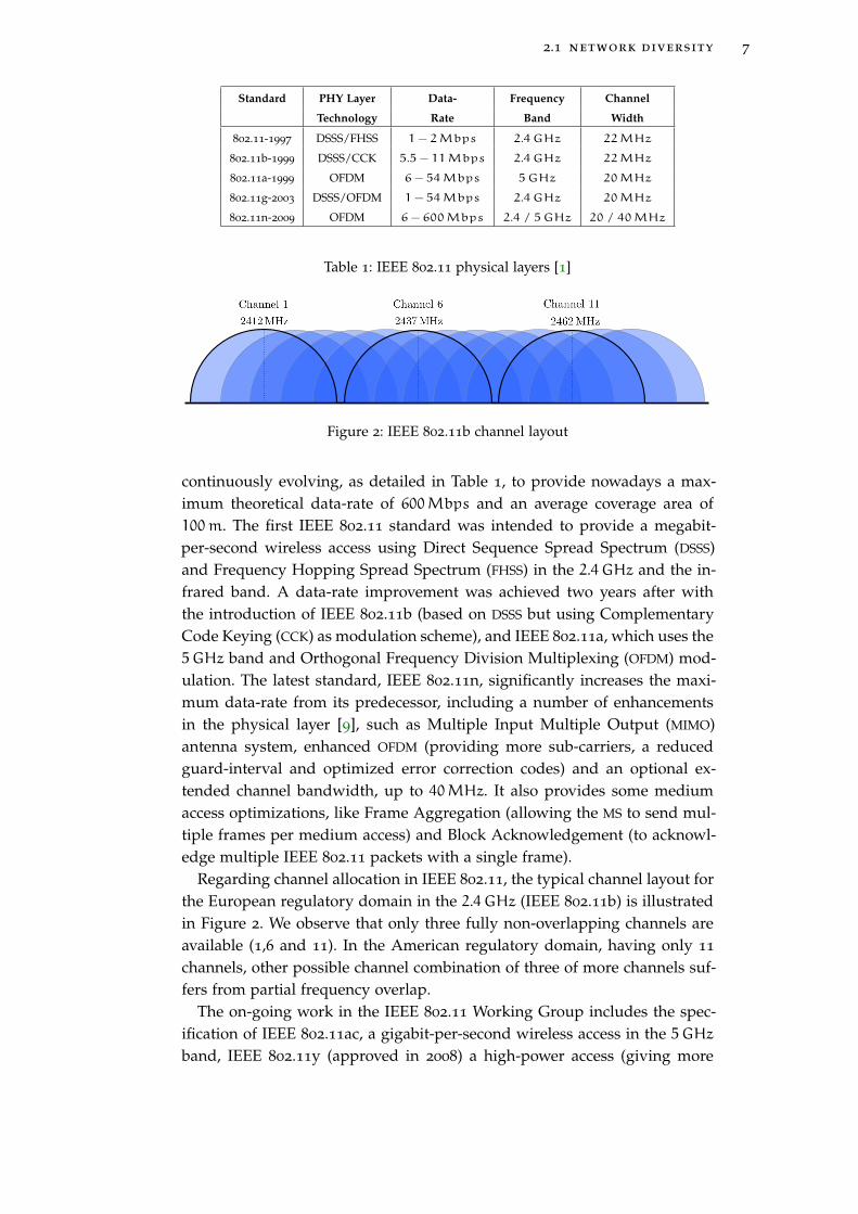
continuously evolving, as detailed in Table 1, to provide nowadays a max-imum theoretical data-rate of 600 Mbps and an average coverage area of100 m. The first IEEE 802.11 standard was intended to provide a megabit-per-second wireless access using Direct Sequence Spread Spectrum (DSSS)and Frequency Hopping Spread Spectrum (FHSS) in the 2.4 GHz and the in-frared band. A data-rate improvement was achieved two years after withthe introduction of IEEE 802.11b (based on DSSS but using ComplementaryCode Keying (CCK) as modulation scheme), and IEEE 802.11a, which uses the5 GHz band and Orthogonal Frequency Division Multiplexing (OFDM) mod-ulation. The latest standard, IEEE 802.11n, significantly increases the maxi-mum data-rate from its predecessor, including a number of enhancementsin the physical layer [9], such as Multiple Input Multiple Output (MIMO)antenna system, enhanced OFDM (providing more sub-carriers, a reducedguard-interval and optimized error correction codes) and an optional ex-tended channel bandwidth, up to 40 MHz. It also provides some mediumaccess optimizations, like Frame Aggregation (allowing the MS to send mul-tiple frames per medium access) and Block Acknowledgement (to acknowl-edge multiple IEEE 802.11 packets with a single frame).

Regarding channel allocation in IEEE 802.11, the typical channel layout forthe European regulatory domain in the 2.4 GHz (IEEE 802.11b) is illustratedin Figure 2. We observe that only three fully non-overlapping channels areavailable (1,6 and 11). In the American regulatory domain, having only 11

channels, other possible channel combination of three of more channels suf-fers from partial frequency overlap.

The on-going work in the IEEE 802.11 Working Group includes the spec-ification of IEEE 802.11ac, a gigabit-per-second wireless access in the 5 GHz

band, IEEE 802.11y (approved in 2008) a high-power access (giving more


MS

MS

MS IBSS

IBSS

IBSS

(a) IBSS Mode

AP<<SSID>>

MSMS

BSS

MSMS

(b) Infrastructure Mode

Figure 3: IEEE 802.11 deployment modes

than 5 km range) in the 3.7 GHz band and IEEE 802.11ad, a very-high data-rate access in the 60 GHz band, mainly intended for a multimedia homewireless access.

2.1.1.1 Deploying IEEE 802.11

The main building block of an IEEE 802.11 network is defined by the BasicService Set (BSS), consisting in a group of stations communicating together.The area where the communication takes place is identified as the BasicService Area, which is conditioned by the wireless medium characteristics(i.e., path-loss, fading, interferences). In order to communicate within a BSS,two different approaches exist (see Figure 3): the Independent Basic ServiceSet (IBSS) (or adhoc) mode and the Infrastructure Mode.

independent bss mode Stations communicate directly with each otherwhen they are within a common coverage range. The adhoc designation is re-lated to the fact that this kind of networks are designed for specific purposesand usually for a sporadic or opportunistic usage. Commonly, when usingan adhoc topology, one of the nodes has access to the Internet, so the othernodes in the network without an Internet connection may use the formernode as a relay to reach the public network.

infrastructure mode In this case, an AP bridges the MS connectedthrough the wireless medium with other hosts connected to a wired Ether-net link, called the Distribution System (DS). This kind of architecture pro-vides several advantages. First, it allows extending the coverage of a wirednetwork to a large number of MS connected to different AP. Differently fromIBSS, in the infrastructure mode the BSS is defined by the radio coverage ofthe AP, which is normally located in a fixed position, giving a stable coveragearea, allowing scalability. Additionally, the AP may buffer frames targeted to


AP<<SSID>>

MS

MS

AP<<SSID>>

AP<<SSID>>

Distribution System

MS

ESS ESS ESS

Internet

Figure 4: The Extended Service Set

an MS, allowing it to enter in Power Saving Mode (PSM) mode and save ev-ergy by switching-off the MS radio circuits (energy considerations for IEEE802.11 are given in Section 2.1.4). In order to achieve a larger coverage area,several BSSs may be chained together using a backbone network and con-ceiving an Extended Service Set (ESS). The main feature offered by an ESS

is that an MS can send/receive frames to/from any other MS, even thoughthey belong to different BSS. In an ESS all BSS are identified with a commonService Set Identifier (SSID). Figure 4 illustrates a typical ESS. In this case, theAP is responsible for locating the MS in the ESS and deliver frames to its finaldestination.

security in ieee 802 .11 In both modes, the standard provides a setof security mechanisms for authentication and encryption. Originally, theWired Equivalent Privacy (WEP) was based on using a common shared keyfor all MS in the network. Since WEP suffered from several weaknesses en-abling users to easily crack the network key, the IEEE has rapidly proposedIEEE 802.11i, including the Wi-Fi Protected Access (WPA) and WPA2 pro-tocols, providing stronger encryption techniques, evolved pre-shared keyauthentication and centralized authentication based on Remote Authentica-tion Dial-In User Service (RADIUS) servers and the Extensible AuthenticationProtocol (EAP).

2.1.1.2 Community Networks

The concept of CN has been developing in the last years in order to pro-vide ubiquitous WLAN coverage in urban areas. These networks differ fromwell-known WLAN hot-spot, metropolitan or municipal networks which onlycover a number of public places and point-of-interests around different cities(e.g., train stations, transportation hubs, bars, shopping malls) requiring for


Internet

CN SSID 1

Private SSID 1

CN SSID 1

Private SSID 2

ISP 1

ISP 2

ISP 3

CN SSID 2

Private SSID 5

CN SSID 3

Private SSID 4

CN SSID 3

Private SSID 3

CN SSID 2

Private SSID 6

Figure 5: A common CN deployment

special subscriptions to access the Internet. The CN concept is based on ex-tending the usage of existing IEEE 802.11 residential networks. In CN, theInternet Service Provider (ISP) gives to each customer a "box", which con-tains an Asymmetric Digital Subscriber Line (ADSL) modem, a router andan IEEE 802.11 AP. This box typically provides users with an Internet ac-cess through a Network Address Translation (NAT). These AP are capable ofbroadcasting multiple network identifiers, enabling users to share their ADSL

access with other customers of the same ISP using a common open-systemauthentication network identifier, the CN SSID. In a common use case, whena user is within the range of his own AP, the secured SSID, implementingWEP or WPA, is used. Whenever a user is out of range of his own AP, he canassociate to a shared CN AP that broadcasts the CN SSID. Then, in order toaccess the Internet, the user must provide his own identifiers through anHypertext Transfer Protocol Secure (HTTPS) captive portal. A common CN

deployment is depicted in Figure 5, where different ISP provide a CN accessto their subscribers, who also manually configure a private secured SSID.

This concept of sharing private broadband ADSL accesses was originallyproposed by FON1, who has been deploying its platform using a specialWLAN AP that users can plug to their routers at home. In France, wirelessCN have been increasingly deployed by the subscribers of four of the mostimportant ISP, counting around 13 millions AP: Free (claiming over 4 millionAP), SFR (claiming over 4 million AP), Bouygues Telecom (claiming over 700

thousand AP) and, very recently, Orange (claiming over 4 million AP).In those CN, there is a concern about the incentive scheme to encourage

users to share their IEEE 802.11 access. Several authors have designed com-plex incentives and credit-based schemes, like Manshaei et al. [10], who

1 http://www.fon.com

http://www.fon.com


RC20001986

GSM1992

GPRS1997

EDGE1998

UMTS2000

HSPA2002

HSPA+2007

LTE2008

LTE-Adv2011

1G 2G 3G 4G

Figure 6: Cellular network evolution

derived an incentive scheme using a game theoretical approach and Ai etal. [11], who proposed a credit-based scheme, where users earn credits forsharing bandwidth. In practice, the incentive scheme of the FON CN is basedon three user profiles that are chosen upon the first registration on the net-work. The Alien users are those who do not share their IEEE 802.11 accessbut still want to get connected to other AP without paying; the Bill users arethose that sell their access using a time-based pricing and share the earningswith FON; finally the Linus users are those that fully share their access with-out asking for money. Regarding the CN operators in France, there is notcomplex pricing and incentive scheme, since users willing to access the CN

can do so only if they share their own Internet access with other subscribers.In this case, the user can only access the CN belonging to his own ISP.

2.1.2 Cellular Networks

2.1.2.1 Technological Evolution

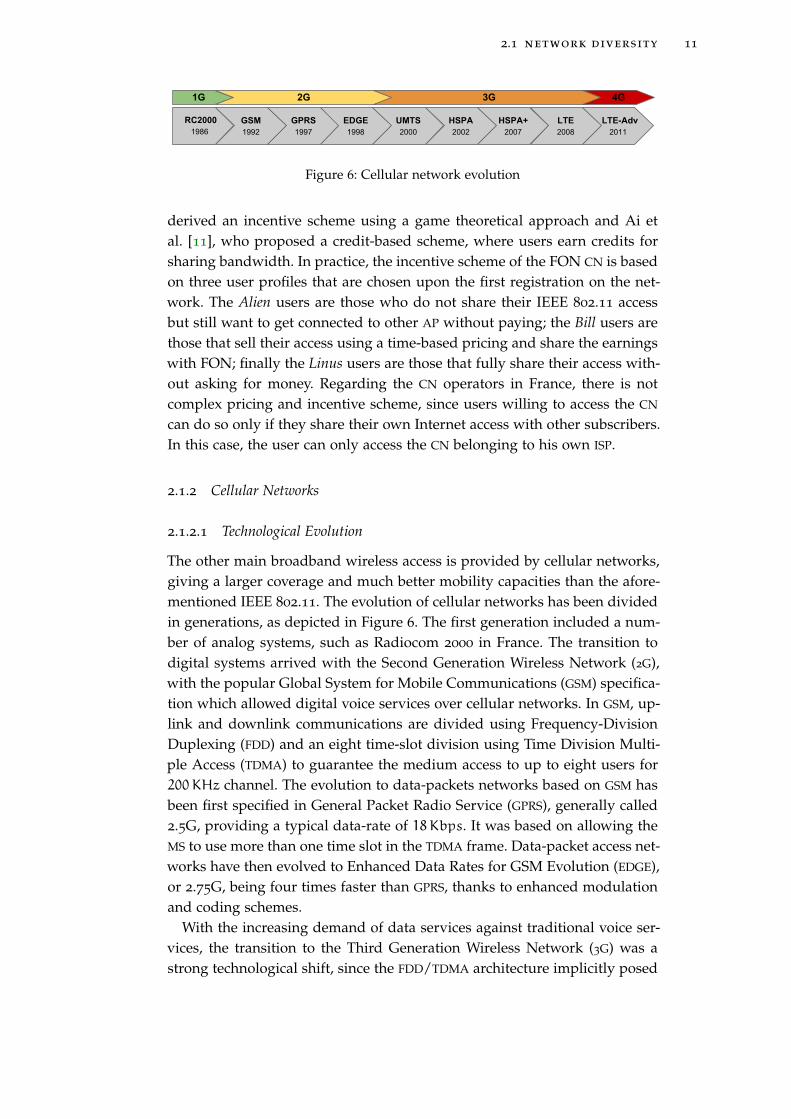
The other main broadband wireless access is provided by cellular networks,giving a larger coverage and much better mobility capacities than the afore-mentioned IEEE 802.11. The evolution of cellular networks has been dividedin generations, as depicted in Figure 6. The first generation included a num-ber of analog systems, such as Radiocom 2000 in France. The transition todigital systems arrived with the Second Generation Wireless Network (2G),with the popular Global System for Mobile Communications (GSM) specifica-tion which allowed digital voice services over cellular networks. In GSM, up-link and downlink communications are divided using Frequency-DivisionDuplexing (FDD) and an eight time-slot division using Time Division Multi-ple Access (TDMA) to guarantee the medium access to up to eight users for200 KHz channel. The evolution to data-packets networks based on GSM hasbeen first specified in General Packet Radio Service (GPRS), generally called2.5G, providing a typical data-rate of 18 Kbps. It was based on allowing theMS to use more than one time slot in the TDMA frame. Data-packet access net-works have then evolved to Enhanced Data Rates for GSM Evolution (EDGE),or 2.75G, being four times faster than GPRS, thanks to enhanced modulationand coding schemes.

With the increasing demand of data services against traditional voice ser-vices, the transition to the Third Generation Wireless Network (3G) was astrong technological shift, since the FDD/TDMA architecture implicitly posed


a performance limit. This technological shift, the Universal Mobile Telecom-munications System (UMTS), is based on Wideband Code Division MultipleAccess (WCDMA), an evolution of the Code Division Multiple Access (CDMA)technique, which required a completely new network deployment, i.e., newbase stations and frequency allocations. In WCDMA, instead of using narrowfrequency channels like in GPRS/EDGE, a larger channel of 5 MHz is used.Then, communications are based on spread spectrum, so each MS uses dif-ferent codes to allow multiple access. This new technique allows a theoreti-cal maximum data-rate of 384 Kbps, which enabled new online applicationsand a more fluid web-browsing. However, the increasing demand for band-width (mainly related to audio and video applications) pushed the evolu-tion of UMTS to High Speed Packet Access (HSPA), called the 3.5G, includingHigh Speed Downlink Packet Access (HSDPA) and High Speed Uplink PacketAccess (HSUPA). HSDPA allows a maximum downlink data-rate of 14 Mbps

by providing some enhancements from its predecessor, like a shared chan-nel transmissions, higher rate modulations and shorter transmission timeintervals. Regarding HSUPA, a new transport channel is defined, namely theEnhanced Dedicated Channel (E-DCH), giving a maximum uplink data-rateof 5.8 Mbps. A further evolution has been designed in the Evolved HighSpeed Packet Access (HSPA+), including MIMO and higher modulation rates,providing 84 Mbps and 10.8 Mbps in the downlink and uplink respectively.

Even if HSPA and HSPA+ were designed to provide very high data-rates,these technologies are limited in the distance in which data can be delivered,since the symbol duration decreases with the increasing data rate, becom-ing much smaller than the multipath distance, hindering the data retrieval.Additionally, another limitation is related to the architecture of the core net-work, which is not an all-IP architecture, forcing a co-existence with legacyvoice circuits and gateways.

The 3rd Generation Partnership Project (3GPP) started to define the require-ments for a new generation of mobile communications, the Fourth Genera-tion Wireless Network (4G), establishing a peak data-rate of 100 Mbps forhigh speed mobility and up to 1 Gbps for low speed mobility or static users.In this direction, the Long Term Evolution (LTE) standard has been releasedin 2008. However, it does not still satisfy the requirements imposed for a4G technology. For that reason, LTE is commonly referred to as 3.9G, evenif it is commercially referred as to 4G. LTE can provide up to 300 Mbps inthe downlink and 75 Mbps in the uplink, with a very low latency (5 ms inoptimal conditions) and supporting high mobility speeds, up to 500 km/h.It uses the Orthogonal Frequency-Division Multiple Access (OFDMA) mech-anism for multiple medium access, supporting both FDD and Time-DivisionDuplexing (TDD) with variable channel bandwidth, from 1.4 MHz to 20 MHz

(recall that a fixed 5 MHz channel was used in 3G systems).The first 4G standard has been finally defined in the LTE-Advanced speci-

fication, allowing gigabit-per-second data-rates by including carrier aggrega-


tion, enhanced MIMO and relay nodes, providing better performance at thecell edge.

2.1.2.2 Current Deployments

Mobile phones penetration rate has surpassed 85 % in 2011 [12], being morethan 100 % in some regions like Europe and the Americas, giving almost6 billion subscribers worldwide. Moreover, after the transition to HSPA thevolume of mobile data has considerably increased (surpassing the amount ofdata generated for voice-based services). Nowadays, more than 900 millionusers have access to broadband wireless accesses through a 3G technology. Inparallel, there has also been a great expansion of the mobile devices market,giving more than 3000 different mobile device models (supporting HSPA)that have been launched in the last years.

To respond to this demand, worldwide network operators have been de-ploying new networks. The current deployment of cellular networks is inpractice a mixture of technologies belonging to different generations. In mostcountries, voice-based services are still carried out using the GSM network,covering nowadays the 90 % of the world population [13]. Regarding the de-ployment of worldwide data-packet networks, we find that HSPA is the mostused technology, since all the 3G commercial deployments have launchedthe HSPA service. The mainstream on the deployment is marked by the im-plementation of HSPA+, giving a total of 234 commercial networks in 112

different countries (in July 2012 [13]). However, there is also a fast develop-ment of LTE in parallel with HSPA+. This is because networks operators havestill to amortize their 3G infrastructure and maximize benefit before shift-ing to LTE, that will require important investments. There are currently 89

commercial LTE deployments in 45 different countries, expecting up to 150

deployments for the end of 2012.

2.1.3 Other Wireless Technologies

Even if the current wireless heterogeneous environment is dominated by amixture of cellular technologies and IEEE 802.11, there are other wirelesstechnologies that are also embedded in most mobile devices. First, the Blue-tooth [14] technology, operating in the 2.4 GHz ISM band, has been originallydesigned to provide wireless connectivity for data sharing among devices(without any infrastructure) over short distances at relatively low data rates,forming a WPAN. Common usages of Bluetooth include file sharing and mes-saging between smartphones and computers, peripheral pairing (e.g., head-sets, input devices, remote controls) and and Internet connection sharingbetween smartphones and laptops (also called Bluetooth modem). Bluetoothhas been evolving over the last years and is able to provide, in its latest ver-sions (v3.0 and v4.0), up to 24 Mbps, which is comparable to the commondata-rates obtained in IEEE 802.11.


The IEEE 802.15.4 [15] standard has been conceived to provide low datarates (up to 250 Kbps), short range and low energy-consumption communica-tions. Its most popular applications are the Wireless Sensor Networks (WSN)and the Internet of Things (IoT). Even if this technology is not stronglypresent in current mobile devices (e.g., laptops, smartphones, tablets), ithas been recently reported2 the launch of a 802.15.4-enabled Android smart-phone, also providing an IEEE 802.11, a UMTS/HSPA and a Bluetooth inter-face.

Finally, the IEEE 802.16 family of protocols, known as Worldwide Inter-operability for Microwave Access (WiMAX) has been designed to offer bothfixed and mobile wireless communications at high data-rates, up to 40 Mbps

with a very large coverage range. Even if it is currently part of the 4G spec-ification, it did not meet the UMTS and HSPA success. However, there existsa large number of deployments worldwide, serving around 20 million usersin 20113.

2.1.4 Energy Consumption of Wireless Interfaces

Energy efficiency of mobile devices has become a major issue in the designof modern mobile communication devices, since the improvement of batterytechnologies has not followed the exponential growth of mobile devices andsystems performance [16]. As stated earlier in this chapter, mobile devices,and especially smartphones and tablets, are equipped with a great numberof wireless interfaces and have the ability to run several applications at thesame time, demanding a huge amount of energy. Moreover, the miniaturiza-tion of mobile devices still limits the size of batteries, which have not greatlyimproved their energy density (measured in Wh/l), commonly providing atotal energy of 1500 Wh for a typical smartphone battery, giving less thanone day of autonomy for a normal usage. If we consider a multi-interfacesmartphone (i.e., having at least IEEE 802.11, 2G/3G/4G and Bluetooth wire-less radio), in a common use case, the radio interfaces contribute, in aver-age, to the 58 % of the total energy consumption of the device [17]. Notethat this contribution may increase if multiple interfaces are simultaneouslyused (multi-homing). We detail in this section the differences, in terms of en-ergy consumption and operating modes of the two most popular broadbandwireless technologies: 3G cellular and IEEE 802.11 networks.

2.1.4.1 UMTS/HSPA

As explained in [18], an MS communicating through a UMTS/HSPA interfacetransits between three different operating states, as listed below:

2 http://www.taztag.com/

3 http://www.wimaxforum.org/news/2866

http://www.taztag.com/

http://www.wimaxforum.org/news/2866


DCH

Idle for

Idle for

Q > Threshold

FACHPCH

Tx/R

x any

dat

a

(a) Carrier 1

DCH

Idle for

Idle for

Tx/Rx any data

Q > Threshold

PCH FACH

(b) Carrier 2

Figure 7: RNC state machines

• Paging Channel (PCH): No radio resource is allocated to the MS sinceno Radio Resource Control (RRC) connection exists.

• Forward Access Channel (FACH): A RRC connection is established with-out dedicated channels, limiting the bandwidth up to a few kbps.

• Dedicated Channel (DCH): An RRC connection is established and a ded-icated channel has been allocated, giving a high data-rate access to theMS.

The power consumption at each state depends on the particular MS hard-ware, but in all cases the PCH is the less consuming state and DCH the mostconsuming state (see Table 4). However, the logic to transit among thesestates, i.e., the state machine, is not managed by the MS but by the RadioNetwork Controller (RNC) in the network side, which is responsible for con-trolling a set of base stations (or NodeB in the 3GPP nomenclature). Then,different network operators may implement different configurations for thestate machine, leading in a different energy consumption for the same usagefor a given MS.

Two example of state machines are given in [18] for two of the most popu-lar carriers in the USA. Figure 7 illustrates these state machines. In the caseof Carrier 1, each time an MS in the PCH state has to establish an RRC connec-tion to send or receive data, it switches to the DCH state to exchange packets.Then, it keeps staying in this state if the packet exchange continues or, inthe case it becomes idle for an inactivity timer of T1 seconds, it switches tothe FACH state, which consumes less power but provides lower bandwidththan DCH as well. The MS then continously monitors the uplink and down-link packet queue (Q) and if its length becomes larger than a threshold, itswitches again to the DCH state to exchange packets at a higher bandwidth.On the other hand, if the MS remains idle in FACH for an inactivity timer T2,it comes back to the idle state (PCH). A more conservative state machine isimplemented in the RNC of Carrier 2. In this case, an MS being in the PCH

state first switches to the FACH state for any RRC connection request. If a


Figure 8: 3G state transitions for a Skype test-call

high throughput is demanded, it then switches to the DCH state. The inac-tivity timers T1 and T2 follows in this case the same logic than for Carrier1.

We performed an experiment to analyze the transitions of a 3G state ma-chine, as illustrated in Figure 8 [19]. We have obtained this trace by perform-ing a Skype test call in an HTC Dream smartphone using the SFR 3G networkand logging the activity of the MS using PowerTutor [20]. We can observe inthis trace that once the call ends at time 75 s, the MS remains in the DCH stateand switches to the FACH state at time 95 s. Then, 10 s after the transition tothe FACH, the MS becomes idle (transition to PCH).

The state machine is set by the network because it is the network oper-ator who has to efficiently manage its limited wireless resources, i.e., thededicated channels. The network operator can set the logic of the state ma-chine, values for T1 and T2 and the queue threshold. In the state machinespresented in [18], these parameters are set as detailed in Table 8. Note thatthere is a trade-off while assigning dedicated channels. In order to negoti-ate a transition to a DCH, several signalling packets have to be exchangedbetween the MS and the network, which roughly takes 2 s. An MS willingto consume a low amount of energy may request a DCH transition everytime there is some data to exchange and go immediately to the FACH orPCH state (i.e., release the DCH channel) without waiting for an inactivitytimer. However, in this situation the user performance is strongly degradedsince there is a signalling overhead caused by multiple negotiations of a DCH

channel. On the other hand, if the MS wants to maximize the performance,it should always remains in the DCH state, but in this case the negative im-pact is twofold. First, a high energy consumption may be observed and sothe MS battery autonomy is reduced. Second, the network operator may runout of wireless resources and so a great number of users may not be able toperform RRC connections.


Parameter Carrier 1 Carrier 2

T1 (s) 5 6

T2 (s) 12 4

Queue Threshold (bytes) 475 119

Table 2: State machine parameters

SLEEP

TX

IDLE

RX

Figure 9: WLAN state machine

2.1.4.2 IEEE 802.11

Differently from UMTS/HSPA cellular interfaces, in IEEE 802.11 the operationmode is much simpler and the state transitions are exclusively managed bythe MS, i.e., there is not a centralized entity (like the RNC in cellular networks)affecting the energy consumption of the device. Figure 9 illustrates the dif-ferent states and transitions for a WLAN interface [21]. During an active com-munication, the interface enters in the transmit (TX) and receive (RX) modeintermittently. If no transmission is active, the MS remains IDLE. Addition-ally, if the interface supports the PSM it can enter in the SLEEP mode, thatconsumes very low energy (see Table 3). When being in such state, the MS

switches its circuits off and requests the AP to buffer its incoming packets.Then, the MS will periodically wake up to receive AP beacons and will lookfor a Traffic Indication Map (TIM) that announces buffered packets for theMS. The transition to the SLEEP mode is usually performed after a timeout(an analysis of different PSM strategies can be found in [22]).

2.1.4.3 Empirical studies and preliminary observations

Several studies exist in the literature trying to characterize how the differ-ent wireless interfaces impact on the global energy consumption of an MS.Petander [23] proposes an overview of energy consumption in terms of thebattery drain (measured in percentage) while using the IEEE 802.11 (WLAN)and the 3G (UMTS) interfaces in an HTC Dream smartphone. Some exper-iments are carried out by varying the traffic load and the signal strengthbetween the MS and the AP or cellular base station. Results show that even if


WLAN State Nokia N810[21] HTC G1[21] Nokia N95[21] Nokia N90[26]

SLEEP 42 68 88 40

IDLE 884 650 1038 800

TRANSMIT 1258 1097 1687 2000

RECEIVE 1181 900 1585 900

Table 3: Power consumption (mW) of WLAN states

3G State N/A[17] N/A[26] Nokia N95[24] HTC TyTN II[18]

PCH < 18.5 19 282 0

FACH 370-740 555 549 400-460

DCH 740-1480 1100 742 600-600

Table 4: Power consumption (mW) of 3G states

UMTS consumes more energy per unit of data (between 0.2 % and 2.8 % perMB), both interfaces slightly consumes the same amount of energy per unitof time (around 0.01 % per second). Xiao et al. [24] proposed a measurementanalysis of YouTube video streaming using both UMTS and WLAN interfacesand different scenarios (e.g., progressive download and view, download firstplay next, local playback). The authors observe that in the case of UMTS,even if the video download is finished and the MS only plays the video, thepower consumption does not immediately decrease, leading to a higher to-tal energy consumption compared to WLAN. This is caused by the effect ofcellular networks inactivity timers (see Section 2.1.4.1). We proposed in [19]an evaluation study of energy consumption of different mobile applicationsusing 3G (UMTS/HSPA) and WLAN interfaces in an Android MS. In particular,these measurements have been performed using PowerTutor [20], a real-timepower estimation tool that allows tracing the instantaneous energy consump-tion of the different components of the MS (e.g., procesor, screen, WLAN, 3G,Bluetooth, GPS). As in [24], we have also observed the effects of inactivitytimers in 3G, especially when doing web-browsing, since during the idle timebetween two web page requests (i.e., the reading time) the MS is not capableof reducing the 3G power consumption. More particularly in [25], Haveri-nen et al. study the energy consumption of always-on applications (basedon keep-alive message exchanges) using UMTS. They show the impact of in-activity timers and keep-alive frequency, proposing some configurations toboth parameters to mitigate this negative impact on energy efficiency.

2.1.5 Discussion

This panoply of wireless technologies are commonly present in urban areas,giving multiple access possibilities to mobile users. In particular for Internetaccess, IEEE 802.11 and 3G networks appear as the most convenient wireless

2.2 related work on wireless diversity evaluation 19

accesses in urban areas. In order to analyze their coexistence and the possi-bility of simultaneously using both interfaces, there has been in the last yearsthe necessity of exploring and evaluating the wireless deployments. Theseevaluation studies were usually taken as an input to design and evaluatenew protocols aiming at optimizing the user experience while using thosenetworks.

In the context of this thesis, a fine-grained knowledge of the wireless envi-ronment and the collaboration between different technologies help to betterunderstand the drawbacks and limitations of current deployments and alsoto identify the opportunities and challenges for optimizing those networks.We particularly focus on optimizing IEEE 802.11 AP discovery in Chapter 3

and the decision-making processes for network selection in Chapter 4.In the following, we present past evaluation studies of wireless diversity

so as to motivate the development of the Wi2Me platform, a new wirelesssensing tool that allow characterizing not only the presence and performanceof wireless networks but also their limitations for mobile users.

2.2 related work on wireless diversity evaluation

In this section, we present the related work on measurement and evaluationstudies aiming to characterize wireless networks in urban environments, in-cluding the existing tools and applications to perform such studies. Regard-ing WLAN deployments, we focus not only on measurement studies for openAP deployments in urban areas but also for research dedicated networks, thathave been specifically deployed to analyze the performance of IEEE 802.11

under different usage conditions. However, in the study that we present inSection 2.4, we focus on open urban WLAN deployments, particularly in CN

and their coexistence with operator-based cellular networks.

2.2.1 Evaluation Studies

In [2], Bychkovsky et al. propose an evaluation study of IEEE 802.11 AP de-ployments in urban areas to provide network connectivity for moving vehi-cles. This study consisted in 290 hours of evaluation of existing urban WLAN

deployments using Linux-based computers with an IEEE 802.11 card and a5.5 dBi antenna and a Global Positioning System (GPS) device installed in sev-eral vehicles. These computers were responsible for discovering the availablenetworks, associating to a (good) candidate AP, obtain an IP address, ping aremote server and finally attempt to upload data through TCP connections.During one year, nine vehicles have been moving around some urban areasof Boston and Seattle (USA), discovering more than 32.000 AP and associat-ing to more than 5.000 AP. However, since their system was only capable tojoin open WLAN, i.e., without any authentication mechanism at the MediumAccess Control (MAC) layer, they could only successfully ping their remote


Median time between AP association and IP address acquisition 3 s

Median time between AP association and first AP ping 8 s

Minimum / Average / Maximum Scan delay 120/750/7030 ms

Minimum / Average / Maximum Association delay 50/560/8970 ms

Average time between two successful associations 75 s

Average time between two successful end-to-end connections 260 s

Median connectivity duration to an AP 13 s

Median AP coverage 96 m

Average packet delivery rate 78 %

Median per-connection throughput 30 KB/s

Median per-connection uploaded data 216 KB

Table 5: General results [2]

server in only 20 % of the connections, i.e., the 3 % of the discovered APs. Us-ing the traces collected during these connections, the authors evaluated thenetworks using different performance metrics as given in Table 5. For mov-ing vehicles, they have observed very short connection durations (in median13 s) allowing to upload 216 KB in median.

Since this study focused on wireless connectivity for vehicles, the authorsprovided a set of metrics to analyze the impact of speed on the connectionperformance. They find that the number of successful associations to an AP

is uniform up to 60 km/h. Above this speed, they observe a very few numberof connections. The connection duration linearly decreases with an increas-ing speed, up to 60 km/h. For greater speeds the connection duration behavesomehow random. However, they observe no correlation between the vehi-cle’s speed and the packet delivery ratio.

With the same aim, Balasubramanian et al. [27] study the potential forexisting WLAN to provide connectivity to moving vehicles. Instead of inven-torying existing wireless networks like in [2], they focus their attention ontwo particular deployments, VanLAN [28] and DieselNet [29], that have beenspecially conceived to analyze vehicular mobility under IEEE 802.11 deploy-ments. In this case, they perform several measurement studies to collect bea-cons from different AP in both networks so as to analyze, by the means oftrace-driven simulations, the performance of different handover algorithmsseeking to minimize the disruption in IEEE 802.11 connectivity.

In a more recent work, Balasubramanian et al. [3] perform a measurementstudy to analyze the feasibility of offloading users’ connections from cellularto WLAN networks. They conducted measurements in three different testbedin the urban areas of Amherst, Seattle and San Francisco (USA), sensing both3G cellular and IEEE 802.11 networks. They installed a computer carrying anIEEE 802.11b and a 3G modem (HSDPA) in several vehicles. This computerhas a software that is able to scan for networks and transfer fixed amounts


Average 3G availability over the time 87 %

Average WLAN availability over the time 11 %

Average Unavailability using 3G/WLAN simultaneously 5 %

Median 3G TCP throughput uplink/downlink 500/600 Kbps

Median WLAN TCP throughput uplink/downlink 280/200 Kbps

Median 3G UDP throughput uplink/downlink 850/1000 Kbps

Median WLAN UDP throughput uplink/downlink 400/500 Kbps

Average packet loss 3G/WLAN 7/22 %


of data. In Amherst, these computers have been deployed on public buses,performing fixed routes, while in Seattle and San Francisco the mobility pat-tern was random. The results of this measurement study is presented inTable 6. They observed a much higher TCP throughput than in [2]. Thiscould be due to more reduced speeds and because in some cases they con-nect not only to open AP but to other AP they have deployed along the path.The authors analyze, using trace-driven simulations, the offloading capacityof 3G data over WLAN. They estimate that in the 53 % of the locations, at least20 % of the 3G data could be sent/received over WLAN. Moreover, in 9 % ofthe locations all 3G data could be sent over WLAN. The total amount of datathat a user may offload to WLAN not only depends on the availability of AP

but also on the tolerance of users to delay the transmission of some flowsuntil a WLAN becomes available.

A most recent evaluation study analyzing the offloading capacity of mo-bile devices in urban heterogeneous networks is proposed by Lee et al.in [30]. In this study, the authors distributed 100 iPhones to different usersmoving around some metropolitan areas in Seoul (South Korea) during 20

days. These devices ran a especial application, DTap, that records the statis-tics of available WLAN every three minutes and perform connections to openAP to estimate throughput and Round Trip Time (RTT) using the ping com-mand. The analysis of the statistics gives that the average temporal WLAN

coverage for a user is around 70 % while spatially, the area covered is be-tween 10 % and 20 %. Users get connected through a WLAN in average 120

minutes per day with a time between connections of around 41 minutes.They model the connection duration and the interconnection time using theWeibull distribution and evaluate the performance of different offloadingstrategies using trace-driven simulations. The authors estimate that up to65 % of the traffic can be offloaded from 3G to WLAN, giving a maximumenergy saving of 55 %.

A measurement study of WLAN deployments in the city of Chicago (USA)is presented in [4], aiming at collecting a large number of traces to evalu-ate best AP selection algorithms using trace-driven simulations. This study


Downtown Residential Suburban

AP found 797 464 256

Open AP found 78 81 43

AP per scan 2.4 2.0 1.8

Usable AP 53.9 % 100 % 97.7 %

Estimated Bandwidth (KB/s) 60 80 200

Estimated RTT (ms) 22 29 20


is performed in three different urban areas (i.e., downtown, residential, sub-urban), walking around a grid of 1.3 km2. Traces have been collected usingan iPaq handheld with an IEEE 802.11b card. In addition to discover AP,the device estimated the RTT and ran a set of scripts to determine whichport numbers (e.g., HTTP, SMTP, Samba) were open. A summary of the re-sults encountered in this measurement study is presented in Table 7. Theyobserved different performance for different urban areas, achieving the high-est throughput in suburban areas, where the lowest density of AP (i.e., thelowest interference) is found.

Another interesting case of study for urban WLAN deployments is theGoogle Muni WiFi Network4. This is a public accessible IEEE 802.11 meshnetwork in Mountain View, California (USA), covering a 31 km2 urban areawith more than 500 Tropos5 AP, serving up to 2.500 (in 2008 [31]) and most re-cently 19.000 (in 2009 [32]) simultaneous users and daily transporting morethan 600 GB of data at a maximum downlink data-rate of 3 Mbps. Contraryto CN, in which public indoor AP are shared to the public, the Google MuniWiFi Network enters in the category of metropolitan or municipal WiFi Net-works, which commonly consists in a dedicated deployment using outdoorAP deployments which are managed by a governmental institution or a third-party operator. Several municipal deployments exist nowadays all over theworld, specially in Europe and North America. In the case of the GoogleMuni WiFi Network, different authors have performed measurement studiesto analyze its performance under urban mobility patterns. A very completeevaluation of the usage patterns of this network is provided by Afanasyevet al. [31]. Even if this evaluation study does not focus on the radio andwireless aspects, it provides a number of metrics to analyze what users canexpect from the usage of this kind of networks. They distinguish three typesof users. The smartphone users (those holding a handheld or similar device),the hotspot users (those users connecting with a laptop) and the modem users(those users that deploy a high-transmit power equipment at home that con-nects to the Google Muni WiFi Network and converts the wireless signal

4 http://wifi.google.com/

5 http://tropos.com

http://wifi.google.com/

http://tropos.com


into a wired signal that users can access at home using an Ethernet inter-face). Regarding the session duration, in 65 % of the cases modem users getconnected for less than one day, while for hotpot and smartphone users themedian session duration is 30 and 10 minutes respectively. Smartphone usersmainly generate HTTP and TCP traffic while modem and hotspot users gen-erate additional traffic, like Peer-to-Peer, Virtual Private Network (VPN) andinteractive traffic (e.g., streaming, VoIP). The authors however find that thereis an order of magnitude more hotspot users than modem users but even inthis scenario, modem users generate a similar amount of traffic than hotspotusers. Regarding users’ mobility, in a one hour period a smartphone con-nects to six different AP in median. The 10 % most moving smartphones getconnected to 32 different AP. They also observe some oscillations in fixedmodem users who change AP at least once. This could be due to the longrange of the Tropos AP, up to 500 m, which impacts the radio signal andforces a handover on the modem side.

A second measurement study over the Google Muni WiFi Network is pro-posed by Arjona et al. [33]. In this case, the authors analyze the capacity ofthis network to support Voice over Internet Protocol (VoIP) for mobile users.An experimentation campaign was carried out in sub-urban, urban and cor-porative areas around the city using Skype-to-Skype and Skype-to-cellularphone calls. Results show a poor performance of VoIP calls using the GoogleMuni WiFi Network, measured with the Mean Opinion Score (MoS), espe-cially for Skype-to-cellular phone calls. The authors estimate that, in orderto achieve a similar MoS than for cellular network phone calls, the GoogleMuni WiFi network should increase its AP density from 30 to 81 AP/km2,which they estimate as costly as a cellular network deployment.

All these studies show that, in urban environments, users have the pos-sibility to intermittently connect to WLAN while moving. Note that in thesestudies, open AP networks have been generally considered, which at thattime represented a considerable part of the deployment. These deploymentsrepresent now a very low number of AP (only 3.12 % of the AP, excludingCN AP, in our measurement study [34]). This motivated us to perform a com-pletely new measurement study for 3G and WLAN using a new wireless sens-ing tool that allows connecting to multiple CN. In the following, we presentthe existing wireless sensing tools and we propose a new platform Wi2Me,for Android mobiles.

2.2.2 Existing War-driving Applications

Even if the measurement studies introduced in 2.2.1 used ad hoc softwareand hardware platforms to gather the traces from wireless networks, thereare nowadays several publicly available tools to do so, running on different


mobile platforms. These tools are usually referred to as war-driving applica-tions in the literature. In this section, we summarize some of them, mainlythose operating under the Android system, like the Wi2Me platform.

openbmap OpenBMap6 is a free and open source wireless sensing toolfor WLAN AP, cellular base stations (GSM, UMTS, HSPA and LTE) and Blue-tooth devices that aims to build a free accessible data base. It is availablefor Android, Windows Phone and openmoko mobile platforms, providingin a website a limited view of the global traces, including coverage mapsof cellular networks and WLAN AP and a full view for self collected traces(containing location information). In July 2012, the database contained cellu-lar traces from 171 countries and more than 780.000 cells from 604 differentoperators. Regarding WLAN traces, more than 650.000 AP from 57 differentcountries have been inventoried.

sensorly The Sensorly7 project is an Android participatory sensing plat-form that aims at creating a very precise wireless network cartography, show-ing the network coverage for 2G, 3G and LTE technologies for more than 120

network operators in different countries. The application allows mobile usersto manually test the data-rate of different networks, which is then uploadedto the remote Sensorly database, in order to feed the network maps. Regard-ing CN in France, Sensorly allows obtaining an estimation of the positionof individual AP for the four main ISP in France: Free, Orange, BouyguesTelecom and SFR, without providing any information about the overall per-formance of those networks.

wigle Very similar to OpenBMap, the Wigle platform8 is a multi-platformparticipatory sensing tool for WLAN and cellular networks that has been ac-tively gathering traces since 2001. It actually runs on Android mobiles andLinux, Mac and Windows computers, counting more than 125.000 users. InJuly 2012 it counted more than 68 million WLAN AP and 1.5 millions cellularbase stations all around the world, mainly in Europe and North America.They also propose a partial view of the traces and some interesting statis-tics (e.g., evolution of the number of discovered networks and encryptionprotocols over the time).

opensignalmaps OpenSignalMaps9 is an Android application provid-ing similar functionalities than the Sensorly platform but particularly for 3G

networks. The traces are also represented in a dynamic heat-map while giv-ing some metrics to compare two or more network operators in terms of av-erage signal strength, uplink and downlink data-rate and round-trip latency.

6 http://openbmap.org/

7 http://www.sensorly.com/

8 http://wigle.net/

9 http://opensignalmaps.com/

http://openbmap.org/

http://www.sensorly.com/

http://wigle.net/

http://opensignalmaps.com/

2.3 the wi2me platform 25

It also compares, for some cities in USA, United Kingdom, Italy, Germanyand Spain, the network performance compared to the average country orworldwide performance. The OpenSignalMaps database contains coverageand performance information from a large number of countries. The appli-cation also discovers WLAN AP, but these traces are not available online.

2.3 the wi2me platform

2.3.1 Introduction

As it has been previously presented in Section 2.2, existing evaluation studiesof wireless heterogeneous networks provide a characterization of current de-ployments by using ad hoc platforms, i.e., specific software installed in somespecific hardware to discover the networks and evaluate their performance.On the other hand, public available war-driving applications are availablefor different platforms, but, in all cases, even if they can successfully dis-cover wireless networks and locate them in a map, they lack of automaticmechanisms to trigger connections and evaluate the performance of the net-works by downloading and uploading data packets in the background, with-out requiring the intervention of the user. Moreover, the access to the tracesis very limited for the users, since only some predefined metrics are avail-able. Unfortunately, the user has not the possibility to manipulate raw traces(e.g., databases, files) and calculate their own metrics. Moreover, as we haveshown in a first measurement study [35] in Rennes (France), the high den-sity of AP and especially of CN, required for a new sensing tool, capable toanalyze CN in an automated manner.

To reach our goal of analyzing the wireless diversity, we have designedand implemented a new war-driving platform, called Wi2Me. The main goalof this platform is to allow continuous AP and base station scanning andautomatic connection to cellular networks and CN, while gathering all thecollected traces into an internal database. In practice, this platform is com-posed of a common Android core, containing the main functionality and twofront-ends, conforming two application versions: a user version, Wi2Me-User

and a research version, Wi2Me-Research. Both applications are detailed in thenext section.

2.3.2 Design and Implementation

2.3.2.1 Wi2Me-User

The Wi2Me-User version acts as a network manager for common smart-phone users, aiming to automatically connect and authenticate to CN whilemoving. With Wi2Me-User, a mobile user first sets his/her CN accounts (user-name and password) that the application will use to attempt automatic con-


Internet

Server

AggregatedDatabase

TrafficGenerator

Wi2Me Research

Wi2Me User

Post-processing and Analysis

Mobile Station Network Side

Figure 10: Wi2Me Architecture

nection and authentication. Then, he/she simply pushes the "Start" buttonto run the network manager, that will perform scanning, connection andHTTPS authentication. After tracing the scanning, authentication and associ-ation process, once the MS gets connected, it will start tracing the activityof the mobile in a SQLite database. As illustrated in Figure 10, Wi2Me-Userlogs information about the usage of the running applications. For instance,it logs the number of bytes and packets transmitted and received (per appli-cation and for all applications together) over the WLAN interface. It can alsolog the evolution of the TCP connections by registering the state transitionsfor each single connection.

2.3.2.2 Wi2Me-Research

functionalities Wi2Me-Research [36] is intended for participatory sens-ing, i.e., to set up measurement campaigns to discover and deeply analyzethe performance of existing cellular networks and WLAN deployments bytaking in consideration not only CN but any captive portal based network.Differently from Wi2Me-User, Wi2Me-Research allows a very fine-grainedtrace collection, at a higher sampling rate, giving to the application the fullcontrol of the wireless interfaces (i.e., it prevents other applications frommaking use of the interfaces) by using a firewall.

This application performs geo-location, network scanning, automatic con-nection and data traffic generation using the IEEE 802.11 and the cellularinterfaces. It differs from other war-driving applications, since for the bestof our knowledge, it is the first war-driving application that performs auto-matic connection and authentication to existent CN, supporting different CN

providers and captive portal based networks. Wi2Me-Research also allowseasily adding to the application captive-portal authentication algorithms (inJavaScript) for any existing network. The application runs in backgroundmode and logs different events and information in a local SQLite database.

Three main modules define the application’s operation, as shown in Fig-ure 11. A first module obtains the MS position by using the GPS or networklocation services (based on GSM and WLAN positioning). A second module is


Figure 11: Wi2Me-Research modules

responsible for managing scanning, connection and traffic generation over3G, while logging base station information. The third module is respon-sible for managing scanning, connection and traffic generation for WLAN.After a WLAN scanning, the application logs the list of discovered AP, in-cluding for each AP the Basic Service Set Identifier (BSSID), the SSID, the sig-nal strength, the channel number and the supported security capabilities. Ifthe user configures at least one CN account (i.e., username and password),Wi2Me-Research can select and connect to an AP and generate data trafficin order to evaluate the application level performance of the CN. Each timethe application finds a known CN SSID having a signal strength greater thana threshold (by default, −85 dBm), it tries to associate with the AP and auto-matically performs HTTPS authentication using JavaScripts plugins we havedeveloped to this end. Then the application may download and/or uploadfiles of different sizes (50, 100, 250 and 500 KB) from a web server located atTelecom Bretagne. The WLAN connection lasts until the MS finishes transfer-ring all the files or there is a disconnection due to poor radio link quality.If no CN SSID is available, the application attempts a cellular connection andperforms the same file uploads and downloads. During each connection, theapplication logs the current signal strength, the data rate and the number oftransmitted or received bytes.

As one of the goals in developing the Wi2Me application was to havea complete picture as possible of the network state and its performance,we have also monitored the network traffic on the server side. We use aCommon Gateway Interface (CGI) script on the web-server that triggers theTCP connection tracing using the ss command (a socket statistics tool) tomeasure the TCP Congestion Window (CWND), the RTT and the throughput.Additionally, for each connection, all the packets are captured on the serverside using tcpdump. After a measurement campaign the user can upload thetraces (in SQLite) to a remote server via the application. Then, traces fromdifferent users and measurement campaigns are merged in a single SQLdatabase. Finally we use Perl scripts to analyze the traces and compute rele-vant performance metrics. We have also used tcptrace to analyze individualTCP connections.

We have observed that for Wi2Me-Research, the intensive usage of thewireless interfaces and the GPS has a strong impact on the battery autonomy,


Figure 12: Battery drain different scanning strategies

Configuration

Services

ScanningConnection

AuthenticationPinging

Data Transfer

ModelController

View

Core

Wi2Me-ResearchWi2Me-User

Log

Figure 13: Wi2Me MVC model

especially due to WLAN scanning. For that reason, in order to prolong thebattery lifetime, the application is paused if the MS stops moving duringa certain time (by default, 60 s). In order to detect movement, we use theinternal accelerometer, since it consumes much less energy. We illustratethe energy consumption of different scanning strategies in Figure 12, wherethe grey curves (sensor-aided scan) represent the battery drain (in %) fordifferent runs of the application using the accelerometer-based movementdetection. We observe that the usage of the accelerometer allows improvingthe battery duration between 3 h and 10 h (depending on user’s mobility)compared to continuous scanning (green and blue curves).

core implementation Wi2Me-Research was designed to be used byany contributor having an Android smartphone with GPS, WLAN and 3G inter-


Figure 14: Traces database schema

faces. To guarantee scalability, we have used a Model View Controller (MVC)architectural pattern, as shown in Figure 13, that isolates the applicationlogic (the core) and the user interfaces. The View can be a complete client ora simple experimental view. The application’s Controller and Model, belong-ing to the Core module, contain the classes that collect and store the tracesand run in background mode, allowing the user to continue using the smart-phone as long as the other applications do not interact with the networkinterfaces. The Controller contains the configuration classes that allow select-ing different parameters and options for the application. It also contains theServices package which includes all the classes running the main flows andproviding interfaces to the device hardware, e.g., network interfaces, GPS,battery, sensors. The Model contains all the classes that are responsible forapplying the control logic and policies, deciding when and how to performa certain action, e.g., trigger a scanning or a connection, transfer data, logevents. The model classes interact with the Controller services to transformpolicies in specific actions. This allows extending the application functional-ity by just implementing a new Model class or inheriting from the existingone without modifying the Controller services.

The application is completely parametrizable. Some of the possible con-figuration variables are: the time between successive WLAN scans (scanninginterval), the signal strength threshold for attempting a connection, the de-lay to attempt a cellular connection after finding a new cell or the amount ofdata to transfer during a connection.

traces organization When running Wi2Me-Research, the device startscollecting information and organizes it in a database (see Figure 14). Everyinformation collected represents a Trace, e.g., a scanning result, an associa-tion or connection event, an authentication event, a ping result or a connec-tion information. A Trace is composed of a timestamp and the MS location in-formation (altitude, latitude, longitude and speed). Location information canbe provided by either the GPS module or by network interfaces, which givea low-precision location that is used when the GPS is unavailable. For eachconnection information (WiFiConnectionData), scan result (WiFiScanResult)


or ping command (WiFiPing), the application stores AP information in aWiFiAP trace, which contains the BSSID (layer-2 address of the AP), SSID, chan-nel number, signal level (in dBm), the supported security protocols and linkdata-rate (in Mbps). For cellular-related information, the Cell trace storesthe Cell Identifier (CID), the Location Area Code (LAC), the operator nameand code, the signal level (in dBm) and the network type (GSM, GPRS, EDGE,UMTS or HSPA). Regarding the connection information, the application logsthe connection type (download or upload), the IP address and the amount oftransferred data for both WLAN and 3G connections. During a connection, aConnectionData trace is logged every 50 ms. Additionally for WLAN connec-tions, the WiFiConnectionData trace logs the number of received and trans-mitted layer-2 packets and the number of layer-2 retransmissions. All thesetraces are gathered and locally stored in a SQLite database on the smart-phone. Unlike other war-driving applications that store the information inplain text files, we decided to organize traces in a database for scalabilityreasons and to simplify the post-processing phase. Once the application isstopped, it is possible to send the collected traces to our remote server viaan FTP client integrated in the application. This feature allows aggregatingtraces from multiple devices in a central server for off-line processing.

2.4 characterizing wireless networks with wi2me

2.4.1 Experimental Setup

The results presented in this section are based on the data obtained duringtwo measurement campaigns using Wi2Me-Research on Samsung Galaxy S(GT-I9000) smartphones running Android 2.2.1. The first campaign [34], il-lustrated in Figure 15, consisted in a single user walking in the city centerof Rennes, France10 carrying two smartphones. One of the smartphones per-formed WLAN scanning and connected to CN to exchange data while the sec-ond smartphone was scanning every 2 seconds for IEEE 802.11 networks andreceiving cellular beacons, while also performing cellular connections. Theaggregated path length was 34 km and the total experimentation time was10h19. We have gathered traces from 6761 unique APs and 61 unique cellu-lar base stations. The Wi2Me-Research application was configured to alternatebetween downloading and uploading files of increasing size, between 50 KB

and 500 KB.We have also performed a second measurement campaign where we fo-

cused on the performance of TCP connections observed by a mobile user. Inthis case we performed multiple runs in urban areas by connecting to twoCN (FreeWiFi and SFR), as well as several connections to a campus WLAN

network at Telecom Bretagne, called SALSA, an open-system HTTPS captive-portal based indoor network covering the campus. We used Wi2Me-Research

10 A map with the estimated AP locations: http://labo4g.enstb.fr/wi2me

http://labo4g.enstb.fr/wi2me

2.4 characterizing wireless networks with wi2me 31

500m

Figure 15: First measurement campaign

over the SALSA network in order to analyze the impact of handovers on TCPconnections since, in CN, layer 3 mobility is not currently supported and soflows are interrupted after a handover. We performed 291 connections andwe obtained traces from the MS and the server side. In both campaigns, anexternal 7 dBi antenna has been added to the smartphone to maximize AP

discovery and CN connection success rate.

2.4.2 Experimentation Results

2.4.2.1 Topology Discovery

density During the first measurement campaign, we have measured theCN deployment density in terms of the number of discovered AP per scan.A scan is triggered every second while the MS is moving. In Figure 16a, alldiscovered WLAN AP are considered, resulting in a median density of 15 AP

per scan, which indicates a very dense environment. The CN AP use differentIEEE 802.11 physical layers. We observe in Figure 16d that in the case ofFreeWiFi, the MS can reach data rates higher than 54 Mbps, indicating anIEEE 802.11n network. In the case of SFR, we can infer from the traces thatthe MS is connected to the AP in IEEE 802.11b/g mode. Figure 16b showsthat FreeWiFi has a denser deployment compared to SFR and Bouygues. AFreeWiFi user may find more than one AP in 70 % of the scans. In the caseof SFR, this value falls to 40 % and only 25 % for Bouygues. The number ofAP discovered per scan by a user having access to all the CN has a median of3.3, denoting fairly dense community networks.


0

0.01

0.02

0.03

0.04

0.05

0.06

0.07

0.08

0 5 10 15 20 25 30 35 40 45 0

0.1

0.2

0.3

0.4

0.5

0.6

0.7

0.8

0.9

1

Rela

tive F

requency H

isto

gra

m

CD

F

Number of APs per scan

Histogram CDF

(a) Global AP density

0

0.1

0.2

0.3

0.4

0.5

0.6

0.7

0.8

0.9

1

0 1 2 3 4 5 6 7 8 9 10 11 12 13 14 15

CD

F

Number of APs per scan

FreeWiFiNeufWiFi/SFR

BouyguesAll CN

(b) CN AP density

0

5

10

15

20

25

30

35

40

1 2 3 4 5 6 7 8 9 10 11 12 13

Channel D

istr

ibution (

%)

Channel Number

18.7

0.82.7

0.8 0.8

36.1

1.2 1.0

5.7 5.5

25.6

0.2 0.9

(c) AP channel distribution

0

0.1

0.2

0.3

0.4

0.5

0.6

0.7

0.8

0.9

1

0 10 20 30 40 50 60 70 80

CD

F

Data Rate / Mbps

NeufWiFi/SFRFreeWiFi

(d) AP data-rates

Figure 16: Topology discovery metrics

channel overlap We study the AP distribution on the different chan-nels. This is a critical issue, since in IEEE 802.11 adjacent channels partiallyoverlap, causing high levels of interference and frame loss [37]. In currentWLAN deployments, there is a coexistence of different IEEE 802.11 physi-cal layers that use various modulation schemes and channel bandwidth (aspreviously shown in Section 2.1.1). In all the cases, the channel separationis 5 MHz, but in IEEE 802.11b channels are 22 MHz wide while in IEEE802.11g/n, channels typically are 20 MHz wide.

Figure 16c shows the distribution of the AP on different channels. Around80 % of the total number of AP are deployed in the IEEE 802.11b non-over-lapping channels (1, 6 and 11). This result confirms the channel distributionpreviously found in [38] and in our previous evaluation study [35]. To evalu-ate the level of overlapping, two metrics are proposed. Figure 17a shows theCumulative Distribution Function (CDF) of the distance between the chan-nels of all the AP observed in a single scan, called the inter-channel overlap.We found that 45 % of the times the APs overlap with other neighboring APsin the (up to four) adjacent channels, which may produce link degradationand packet loss due to partial overlap (the corresponding cases are shown inred). A four channel separation is needed, since we consider that there areIEEE 802.11b users, that require a 22 MHz wide channel. We observe in Fig-ure 17a that the most likely separation is five channels, which is the case of


0

0.05

0.1

0.15

0.2

0.25

1 2 3 4 5 6 7 8 9 10 11 12 0

0.1

0.2

0.3

0.4

0.5

0.6

0.7

0.8

0.9

1

Rela

tive F

requency H

isto

gra

m

CD

F

Separation between channels

Hist (Ov) Hist (Non-ov) CDF

(a) Inter-channel overlap

0

0.1

0.2

0.3

0.4

0.5

1 2 3 4 5 6 7 8 9 10 11 12 13 14 0

0.1

0.2

0.3

0.4

0.5

0.6

0.7

0.8

0.9

1

Rela

tive F

requency H

isto

gra

m

CD

F

Number of APs in the same channel

Histogram CDF

(b) Intra-channel overlap

Figure 17: Channel overlap metrics

the classical non-overlapping deployment 1-6-11. Then, we define the intra-

channel overlap as the number of APs operating in the same channel. Figure17b shows that in the 55.3 % of the cases a given channel is shared by two ormore APs. Even if most recent AP models implement an intelligent channelselection mechanism to find the most convenient channel, the high AP den-sity, the uncontrolled deployment and the limited spectrum in the 2.4 GHz

band generate an inevitable intra-channel overlapping. These interferencesnotwithstanding, CN are capable of supporting user communications at rea-sonable data rates, as illustrated in the following sections.

2.4.3 End-User Experience in Community Networks

2.4.3.1 General Results

Table 8 summarizes the results obtained in the first campaign, during whichwe have performed 661 connections to two CN (FreeWiFi and SFR) and 17

connections to cellular base stations belonging to a single operator (SFR).Such a difference between the number of connections to CN and cellular basestations is due to the Wi2Me-Research connectivity policy, which attempts aconnection to a CN every time a CN AP having a signal strength greater thana threshold (by default, −85 dBm) is available. Given the high density of CN

AP and the fact that the MS cannot simultaneously connect to both WLAN

and cellular networks, the MS was connected to a CN AP most of the time.We downloaded 158 MB (in 1136 files) and uploaded 125 MB (in 900 files)using CN. We observe different connection success rates among CN operators.In the case of FreeWiFi, a connection attempt succeeds in almost 60 % ofthe cases (510 CN connections over 858 attempts) while a SFR connectionsucceeds only in 30 % of the attempts (151 CN connections over 504 attempts).However, SFR shows a slightly higher average throughput than FreeWiFi. Asshown in Table 8, we have observed higher average and peak throughput incellular than in CN connections. This may be due the low signal strength


Network APs / Connection L2/L3/CN Number of Files Tx/Rx MB Average Throughput Peak Throughput

Cells Attempts Connections (Down/Up) (Down/Up) (Down/Up) (KB/s) (Down/Up) (KB/s)

FreeWiFi 720 858 802/626/510 846 / 675 114.5 / 90.2 51.2 / 61.2 162.9 / 172.4

SFR 908 504 626/410 /151 290 / 225 43.5 / 35.1 65.5 / 41.2 367.9 / 126.5

Cellular 61 17 - 57 / 54 11.9 / 11.6 92.7 / 73.7 381.7 / 225.3

Table 8: Performance results for CN and cellular network connections

received from CN AP, as detailed in Section 2.4.3.3, and CN rate limitationsimposed by ISP as discussed in Section 2.4.3.5.

2.4.3.2 Complementarity between CN and 3G

The MS activity during the first experiment campaign is shown in Figure 18.A cellular base station was available 99.2 % of the time, 45.5 % of the timethe service offered was HSDPA (supporting downlink speeds between 3.6and 14.4 Mbps) and a UMTS access (up to 384 Kbps on the downlink) for therest of the time. Regarding WLAN, a CN AP with a signal level greater than−85 dBm was available 98.9 % of the time. This dense deployment allowedthe MS to have a link layer connection to a CN for 93.9 % of the time.

0 1 2 3 4 5 6 7 8 9 10

Experimentation Time / h

42.4%

47.4%

53.8%

60.5%

83.1%

93.9%

98.9%

99.2%

50KB Upload50KB Download

Internet AccessCN Connection

L3 ConnectionL2 Connection

CN availability3G availability

Figure 18: Smartphone activity during the first campaign

On the other hand, the MS has been successfully connected to the Internetthrough a CN (i.e., at least one packet was successfully received) only for53.8 % of the time. This is mainly due to packet loss during Dynamic HostConfiguration Protocol (DHCP) exchanges or to captive portal authenticationproblems due to poor signal strength.

2.4.3.3 Signal Strength

Figure 20 shows the signal strength distribution for the different CN opera-tors. FreeWiFi and SFR have an equivalent signal strength distribution (inmedian, −80 dBm) while Bouygues has a weaker signal strength probablydue to a smaller gain of the embedded AP antenna or lower transmit power.The low signal strength in CNs is related to the fact that residential APs arecommonly deployed indoor, as their main goal is to cover an apartment or ahouse, reducing the power of the signals received outdoor. This issue is alsoraised in [39], where the authors analyze the impact of verticality of indoorAP in an outdoor usage. However, considering that a 7 dBi gain antenna has


0

0.1

0.2

0.3

0.4

0.5

0.6

0.7

0.8

0.9

1

-90 -85 -80 -75 -70 -65 -60 -55 -50 -45 -40C

DF

Signal Strength / dBm

FreeWiFiNeufWiFi/SFR

Bouygues

Figure 19: Signal strength distribution

been attached to the MS, a larger gain might be needed in both the MS and theAP in order to guarantee a good user experience when connecting to CN ina urban mobility use case. We have also investigated the distribution of thesignal strength during connection and disconnection events. In Figure 20a,we can observe that the median signal strength during a connection attemptis around −76 dBm for both FreeWiFi and SFR. However, successful connec-tions (i.e., those with a successful CN authentication) require a higher signalstrength, giving a median value of −71 dBm for FreeWiFi and −73 dBm forSFR. At disconnection, we obtained a median signal strength of −78 dBm forFreeWiFi and −80 dBm for SFR (see Figure 20b).

0

0.1

0.2

0.3

0.4

0.5

0.6

0.7

0.8

0.9

1

-90 -85 -80 -75 -70 -65 -60 -55 -50 -45 -40

CD

F

Signal Strength / -dBm

FreeWiFi (all)NeufWiFi/SFR (all)

FreeWiFi (successful)NeufWiFi/SFR (successful)

(a) Signal strength at connection

0

0.1

0.2

0.3

0.4

0.5

0.6

0.7

0.8

0.9

1

-90 -85 -80 -75 -70 -65 -60 -55 -50 -45 -40

CD

F

Signal Strength / -dBm

FreeWifiNeufWiFi/SFR

(b) Signal strength at disconnection

Figure 20: Signal strength distributions at connection and disconnection

In order to evaluate the signal strength impact on the download perfor-mance, we have calculated the average throughput and the average numberof link layer retransmissions for different signal strength levels observedin all connections to FreeWiFi during the second measurement campaign.Figure 21a shows the average number of retransmissions per second for dif-ferent signal strength levels. We observe that there is no retransmission forsignal strength levels greater than −60 dBm; for lower levels, the link qualitydegrades, forcing the MS to retransmit packets. Figure 21b shows the relation


between the signal strength and the average throughput. We observe that forstronger signal strengths, the MS reaches the maximum average throughputprovided by the CN (around 100 KB/s). We can also observe that for lowsignal strength levels, between −65 dBm and −80 dBm the throughput is ex-tremely variable, resulting in unstable performance. Observe in Figure 21bthat the maximum achievable throughput is reached for signal strength val-ues greater than −60 dBm. However, such a level of signal strength has beenobserved during less than 2 % of the time, leading to fairly low average datarates in our experimentation.

-5

0

5

10

15

20

25

30

-90 -80 -70 -60 -50 -40 -30

Retr

ies


Retries Std. Dev. Retries Average

(a) Retries vs Signal Strength

-20

0

20

40

60

80

100

120

-90 -80 -70 -60 -50 -40 -30

Thro

ughput / K

B/s


Throughput Std. Dev. Throughput Average

(b) Throughput vs Signal Strength

Figure 21: Signal strength correlations

2.4.3.4 Connection and Disconnection Periods

We analyzed the connection duration and the distance covered by the userwhile being connected to a CN AP. In our campaigns, the MS moves at awalking speed (roughly 1 m/s). In Figure 23 we plot the relation betweenthe distance covered and the connection duration. Most of the points clusteraround the dashed reference line which corresponds to 1 m/s. Figures 22aand 22b show the distribution of the covered distance and the duration of aconnection respectively. We observe a median connection duration of 27.5 s

corresponding to a displacement of 26 m. This result doubles the connectiontime observed in [2]. We observe that the IP disconnection time, i.e., the timebetween a disconnection and a new connection to a CN, has a median of5 s. More precisely, the time needed to establish a layer-2 connection has amedian of 2 s and the time to have a functioning Internet connection after asuccessful layer-2 connection has a median of 3 s. Even if these disconnectiontimes dramatically perturb real-time and interactive applications, they maynot greatly affect applications like email, micro-blogging or browsing, thatmay tolerate a higher latency. Compared to results presented in [2], thanksto the high density of CN, permanent connectivity could be feasible becausemost of the time a CN AP is available. So instead of having the 23 s betweentwo connections calculated in [2], we observe a disconnection time of 5 s

that is only due to protocol latencies and not to the network deployment.


0

10

20

30

40

50

0 20 40 60 80 100 120 140 0

0.1

0.2

0.3

0.4

0.5

0.6

0.7

0.8

0.9

1

Fre

quency H

isto

gra

m

CD

F

Connection Duration / s

Histogram CDF

(a) Connection duration

0

5

10

15

20

25

0 20 40 60 80 100 120 0

0.1

0.2

0.3

0.4

0.5

0.6

0.7

0.8

0.9

1

Fre

quency H

isto

gra

m

CD

F

Distance / m

Histogram CDF

(b) Connection distance

Figure 22: Connection and disconnection metrics

0

20

40

60

80

100

0 20 40 60 80 100

Dis

tance / m

Connection Duration / s

Number of connections 1 m/s Moving

Figure 23: Duration-distance correlation

Note that these 5 s could be significantly reduced by carefully tuning theparameters used in the protocol implementations (e.g., better triggering thelink going down event).

Regarding session continuity, we observed in all CN that the connectionsare interrupted when the MS handovers to a new AP. In the case of FreeWiFi,once associated to an AP, the MS obtains a public IP address which is leasedfor 130 s, but even if the same IP address is used in the new AP, no com-munication is possible. This could be caused by a missing routing updatecausing IP packets to be routed to the wrong AP (recall that in CN, AP arerouters as well). In the SFR CN, the MS is behind a NAT and acquires a privateIP address using DHCP. Then, after a handover, the IP address is no longervalid in the new AP and a complete reconfiguration is needed. In the case ofthe university campus network, called SALSA, all the AP belong to the samesubnet, thus an MS is able to pursue its communication after a transition be-tween two AP. In this case, we observe an uninterrupted download, even ifthe bandwidth is highly degraded when a handover occurs.

2.4.3.5 Transport Layer Aspects

Thanks to the traces collected on the server side, which used TCP Reno, wecan reconstruct individual connections with a good level of detail. We use the


tcptrace utility which can compute, among other parameters, an estimateof the CWND, the value of the TCP Receiver Window (RWND), an estimateof the RTT and of the TCP throughput. Figures 24a and 24b illustrate theevolution of CWND and RWND for one SALSA and one FreeWiFi connectionrespectively, where the MS was downloading the file and it was, therefore,the TCP receiver. Note that in the case of the FreeWiFi connection, RWND isnever a limiting factor as it is always much larger than CWND. Instead, inthe case of the SALSA network (Figure 24a), at times the two windows areidentical, meaning that the application layer throughput is being limited bythe receiver. As we have observed this in multiple connections, we computedthe distribution of the ratio CWND/RWND for FreeWiFi, SFR and SALSA (Fig-ure 24c). As CWND is always lower than RWND the ratio falls in the interval(0, 1]. We observe that in CN, in almost all the cases, the ratio between thetwo windows is lower than 0.2, meaning that RWND is at least five timesCWND. For the SALSA connections, instead, RWND is at most 1.25× CWNDin the 40 % of the cases. This confirms the fact that Figures 24a and 24b arerepresentative of our sample.

As far as handovers are concerned, we have observed that no TCP con-nection was able to continue after a handover in CN. Even in the case ofFreeWiFi, which (at least in some cases) uses the same public IP addressbefore and after a handover, there is no traffic on the server side after thehandover. As one can observe in Figure 25c the same is true on the MS side,even though the received signal strength (Figure 25a) is high. One possibleexplanation is that the IP packets are still routed to the previous AP, pre-venting the TCP connection from working after the handover. In the SALSAnetwork, instead, TCP connections do keep working after a handover but, inmost cases, the TCP sender (i.e., the server in our case) experiences a time-out after a handover, leading to an important reduction in the congestionwindow. Figure 24a shows a typical evolution of the congestion window fora TCP connection of a mobile user in the SALSA network. To quantify thisbehavior, we have calculated the relative delay between the handover andthe reduction of the CWND to at least half its maximum value before thehandover (see Figure 24d). In some cases (less than 20%) the dynamics ofthe TCP connection were such that the congestion window was cut shortlybefore or about the same time as the handover but in 70% of the cases thewindow was reduced during the 4 s following a handover. Given the smallRTT of the TCP connections in the SALSA data set, these timeouts and win-dow reductions do not affect significantly the TCP throughput but such abehavior could decrease the performance in the case of a wide area networkwhere RTT, and competing traffic can be significantly larger. Finally, it isalso interesting to observe that, as shown in Figure 24a, the aforementionedproblems with the RWND limiting the CWND at times, happen right after ahandover. One possible explanation is that the algorithm used by the MS tocompute the RWND is confused by the timeout and the corresponding in-

2.5 mobility issues in community networks 39

0

0.02

0.04

0.06

0.08

0.1

0 10 20 30 40 50 60 70 80 90

MB

yte

s

Time / s

CWND RWND Handover

(a) CWND and RWND (SALSA)

0

0.05

0.1

0.15

0.2

0.25

0.3

0 5 10 15 20 25

MB

yte

s

Time / s

CWND RWND Handover

(b) CWND and RWND (FreeWiFi)

0

0.1

0.2

0.3

0.4

0.5

0.6

0.7

0.8

0.9

1

0 0.2 0.4 0.6 0.8 1

CD

F

CWND / RWND

SALSA

NeufWiFi/SFR

FreeWifi

(c) CWND/RWND Distribution

0

0.1

0.2

0.3

0.4

0.5

0.6

0.7

0.8

0.9

1

-6 -4 -2 0 2 4 6 8 10

CD

F

Relative time to handover / s

(d) CWND reduction delay

Figure 24: CWND and RWND metrics

crease in the RTT, leading to a much smaller RWND. All this shows how, evenif the application-level performance is acceptable in the case of the SALSAnetwork, this could not be the case for a wide area network.

2.5 mobility issues in community networks

During our measurement campaigns, we found a high density of WLAN AP

along our itinerary. One could deduce that there is a potential for a lowcost and high data rate Internet access in urban areas. However, we haveobserved a low received signal strength most of the time (even if an externalantenna has been used); 90 % of the measured signal strength samples arelower than −70 dBm, and 50 % are lower than −80 dBm. This results in shortconnection times, between 10 and 40 seconds, when a user is moving at1 m/s (see Figure 23). This high density also makes the disconnection time(with a median of 5 s) to be only dependent on the protocol latencies sincewhen a handover occurs there is always a candidate CN AP. Thus, while CN

are currently used mainly by static users, they have the potential to offer areliable Internet connectivity to mobile users, provided optimized mobilityprotocols are deployed to support handover between AP. In this way, oncethe current connection with an AP is lost, the MS can switch to another AP

while maintaining its communication. In the following sections, we study


-85

-80

-75

-70

-65

-60

-55

-50

-45

-40

0 5 10 15 20 25 0

5

10

15

20

25

Sig

na

l S

tre

ng

th /

dB

m

Da

ta R

ate

/ M

bp

s

Time / s

Signal StrengthData Rate

Handover

(a) FreeWifi: Power and data-rate

-85

-80

-75

-70

-65

-60

-55

-50

-45

-40

0 10 20 30 40 50 60 70 80 90 5

10

15

20

25

30

35

40

45

50

55

Sig

na

l S

tre

ng

th /

dB

m

Da

ta R

ate

/ M

bp

s

Time / s

Signal StrengthData Rate

Handover

(b) SALSA: Power and data-rate

0

100

200

300

400

500

600

700

0 5 10 15 20 25

0

20

40

60

80

100

120

140

160

180

Pa

cke

ts

Re

trie

s

Time / s

TX Packets

RX Packets

Retries

Handover

(c) FreeWifi: Packets and retries

0

2000

4000

6000

8000

10000

12000

14000

16000

0 10 20 30 40 50 60 70 80 90

0

20

40

60

80

100

120

140

160

180

Pa

cke

ts

Re

trie

s

Time / s

TX Packets

RX Packets

Retries

Handover

(d) SALSA: Packets and retries

0

0.5

1

1.5

2

2.5

3

3.5

4

0 5 10 15 20 25

Ba

nd

wid

th /

Mb

ps

Time / s

Bandwidth Handover

(e) FreeWifi: Throughput

0

5

10

15

20

25

0 10 20 30 40 50 60 70 80 90

Ba

nd

wid

th /

Mb

ps

Time / s

Bandwidth Handover

(f) SALSA: Throughput

Figure 25: Performance metrics for CN and SALSA

the impact of handover on the applications and explain what could be doneto provide mobility support in CN.

2.5.1 Handover impact

A handover, which is deeply studied in Chapter 3, is the process performedby an MS to change AP. It may be triggered by a low signal strength from thecurrent AP or bad link layer performance. A handover consists in discoveringpotential APs operating in the MS radio range and then authenticating andassociating with one of them. Then, IP layer operations may be needed if thenew AP requires that the MS acquires a new IP address.

2.5 mobility issues in community networks 41

Authentication after a handover is one of the critical aspects in CN. Insome cases, when an MS disconnects from a CN AP and re-associates to anew AP of the same CN, HTTPS authentication through a captive portal hasto be carried out again. It means that a user typically enters his login andpassword at each connection with an AP. In our application, no interaction isneeded with the user, scripts perform the authentication on the user behalf.However, it still takes between 1 and 2 seconds, which is unacceptable forseveral applications.

In order to further analyze the handover, we propose to study the impactof handover on a data transfer by making a comparative analysis betweenCN and the SALSA network, where only a layer 2 handover is needed (allAP are on the same subnet). Figure 25 shows the signal strength, the totalnumber of packets transmitted (TX) and received (RX) as well as the linklayer retransmissions (retries) and the bandwidth (on the server side) fortwo individual connections to FreeWiFi and SALSA. We have observed that,in the case of CN, when the MS reaches the limit of its AP coverage area, theMS automatically switches to a new AP. However, in all the cases, we haveobserved that the download is interrupted as shown in Figure 25c. After ahandover (marked with a blue cross), even if a good signal strength is re-ceived from the new AP (see Figure 25a), the RX packets curve from Figure25c stops increasing. On the other hand, we observe exactly the contraryin SALSA, where the MS can always continue the download after a han-dover. Figure 25b shows the data rate and power after handovers (indicatedby a blue cross) while Figure 25d shows that the MS continuously receivesand sends traffic. Figures 25d and 25f also show the number of retries andthroughput. We can see that before each handover, the number of retries in-creases and the throughput decreases. We also observed that, in some cases,the throughput is low for some time after the handover, before the MS canfully exploit the capacity of its new connection. This is the time needed bythe transport layer to adjust its transmission rate to the new capacity of thenetwork.

2.5.2 Predicting a handover

Two optimizations can be set up to reduce the handover impact on appli-cations. First, the handover process can be enhanced, by proposing mecha-nisms at different layers to either better manage the handover or limit theimpact on transport protocols. Second, it might be possible, at least in somecases, to use a (short-term) prediction mechanism to forecast impending dis-connections in order to execute a handover before the link conditions are sig-nificantly degraded. We have observed that, in most cases, shortly before anMS is disconnected from the current AP, the signal strength and the through-put are both decreasing, while the number of link-layer retransmissions in-


0.5

0.55

0.6

0.65

0.7

0.75

0.8

0 1 2 3 4 5 6 7 8 9 10

Pro

b[S

lope <

0]

Time before handover / s

(a) Power Slope Probability

0

0.05

0.1

0.15

0.2

0.25

0.3

0.35

0.4

0.45

0 5 10 15 20

Pro

b[R

etr

ies >

5]


(b) Retries Probability

400

500

600

700

800

900

1000

0 2 4 6 8 10

Ave

rag

e R

TT

/ m

s


(c) Average RTT

Figure 26: Signal strength, retries and RTT before a handover

creases significantly as shown in both FreeWiFi and SALSA connections inFigure 25.

In order to better characterize and therefore better detect an impendinghandover, we have computed three parameters. First, in Figure 26a, we showthe percentage of cases where the short-term trend of the signal strength(slope) is negative as a function of the time before the handover. When thehandover approaches, around 80 % of the times there is a degradation of thesignal strength. Figure 26b the percentage of cases where there are more than5 retries per second. We observe that 5 s before the handover occurs, a highlevel of retries becomes more probable. Finally, in Figure 26c we considerthe average RTT measured on the server before the handover. We observe alinear increase of the RTT when a handover approaches, reaching almost 1 s.

In order to anticipate handover decisions, we could monitor the signalstrength and the number of retransmissions. While link-layer retransmis-sions can be measured only when the MS is sending data, this is exactlythe case where handover anticipation is most important.

2.5.3 Mobility Support in upper layers

If CN operators want to offer seamless connectivity, they need to deploymechanisms to quickly and efficiently handle frequent handovers at layers

2.6 possible evolutions in community networks 43

2, 3 and 4. First, in order to improve the radio link quality and so reducethe handover frequency, CN AP may replace common internal antennas, thathave become popular due the miniaturization of devices, with high-gain ex-ternal antennas. This could reduce the handover frequency and give moretime to the MS to anticipate and prepare the handover. Second, layer 3 mech-anisms are needed to allow users to keep continuous IP-layer connectivitywhile moving. Operators may configure CN AP in a single IP subnet or in aset of geographically distributed subnets (e.g., one for each neighborhood).However, this solution may not scale to the large number of current AP (i.e.,several millions). Another approach is to introduce Mobile IP [40] in the net-work architecture. In this case, each operator may deploy a Home Agent,which allows the MS to continue receiving flows while moving from one net-work to another. Moreover, a single Home Agent for several CN operatorshaving a roaming agreement could allow mobile users to roam between APsbelonging to different communities. Nevertheless, a negative handover im-pact at the transport layer (i.e., layer 4) is observed for both CN and SALSA.In the case of CN, the CWND can never recover due to a network disconnec-tion. In the SALSA network, we observed that the throughput is drasticallyreduced just after and before the handover due to the combination of poorsignal strength and the reduction and later recovery of the CWND. To over-come the impact of handover at layer 4, some solutions already exists, likeFreezeTCP [41], which can prevent the CWND from dropping when a han-dover occurs, provided the appropriate control message can be sent at leastone RTT before the handover takes place.

2.6 possible evolutions in community networks

2.6.1 Managing and Controlling Deployments

The fact that ADSL subscribers can easily share their WLAN access allows, onthe one hand, proposing a simple model to set up a dense network, but,on the other hand, the AP coverage and capacity planning are uncontrolled.Users can place AP and manually set the operating frequency (channel) andthe modulation scheme (IEEE 802.11b/ g/n and different data-rates). Userscan also turn-off and on the AP whenever they want, resulting in a com-pletely dynamic topology. This uncontrolled deployment leads to high levelof interference, limited per AP coverage and relative low network perfor-mance as also studied in [39].

A potential solution would be for CN operators to take control of the radioconfiguration on behalf of their subscribers. First, they could automaticallyselect the AP channel depending on the environment (i.e., neighboring APsand other devices operating in the ISM bands). This is currently implementedin several AP, but since it is not mandatory, users may manually set the chan-nel without having any knowledge of surrounding sources of interference.


Second, operators could dynamically modify the CN AP deployment by re-motely regulating the AP output power (or directly turning them off). This issimilar to cell-breathing techniques in cellular networks. Some cell breathingalgorithms for WLAN have been proposed in [42]. Using such a mechanism,operators may adapt the deployment to the current users needs, possiblyleading to a more energy efficient network as a positive side effect.

2.6.2 Using multiple network interfaces

We have observed in Figure 18 that in urban areas, the density of wirelesscommunity deployments is such that at least one CN AP having a signalstrength greater than −85 dBm is available 98.9 % of the time, which is equiv-alent to the availability of cellular base stations (99.2 %). This should allow auser to use both interfaces at the same time instead of alternating betweenthem. Existing mobile devices use a pre-established connectivity policy (em-bedded in the OS) dictating the use of a single interface at a time for allflows. On the contrary, if using multiple interfaces simultaneously were en-abled, users could implement smart decision-making schemes. In Chapter 4,we survey the decision-making in network selection and propose a multi-objective decision-making problem that we solve using genetic algorithms.

Recent studies try to optimize this deterministic interface selection in or-der to offload cellular data to WLAN networks [30]. Offloading strategiesfocus on reducing the cellular overload by delaying data transmissions untilthe user enters in a WLAN covered zone. As we have shown in the proposedmeasurement study, in a urban environment, WLAN deployments appear tobe highly ubiquitous, therefore a user may have the opportunity to offload asignificant amount of traffic using CN or even to enhance his experience bysimultaneously using both access technologies.

2.7 concluding remarks

In this chapter, we have characterized CN using the Wi2Me-Research appli-cation. This application was designed to periodically scan the radio envi-ronment, connect to IEEE 802.11 AP and cellular base stations and evaluatethe application layer performance. CN are created by millions of users shar-ing their residential AP with other subscribers. Particularly in urban areas,CN have a high AP density, albeit coupled with an uncontrolled deployment.During a CN connection, that we have measured to last between 10 and 40

seconds, we observed different values of throughput for the same signalstrength and vice versa. So that signal strength alone can hardly determinethe application performance. We have also shown that handovers are notsupported in CN, because after changing AP, the application flows are notredirected to the new AP. In a controlled IEEE 802.11 deployment, such asa campus network, a user may change AP without interrupting its commu-

2.7 concluding remarks 45

nication, if handovers are supported at layer 2 and 3. But even in this case,the handover is not transparent for TCP as, in most cases, the congestionwindow is significantly reduced for up to 6 seconds after a handover. Fur-thermore we observed that sometimes after a handover, the TCP receiver isstill limiting the sender window size by announcing a low RWND.

We have shown that mobility support is required in CN because, due to thelimited connection time, handovers are frequent. We also observed that theused protocols to manage handovers are not optimized: the time needed toreconnect a new CN AP has a median of 5 s. To reduce the contribution of theauthentication process on the handover delay, some operators have started todeploy Extensible Authentication Protocol Method for GSM Subscriber Iden-tity Module (EAP-SIM) [43], aiming at automatically authenticating WLAN-enabled smartphones using the GSM Subscriber Identity Modules (SIM) in-stead of using captive portal based authentication. However, in order to stillreduce the handover delay, the MS may reduce the AP discovery latency byoptimizing the scanning algorithm. We address in Chapter 3 the handovermanagement, particularly the AP discovery process in IEEE 802.11.

3H A N D O V E R O P T I M I Z AT I O N S A N D A C C E S S P O I N TD I S C O V E RY I N I E E E 8 0 2 . 1 1

3.1 introduction

The usage of wireless networks has incredibly evolved during the last years.Current mobile users have the possibility to connect to different networktechnologies using multi-interface devices. In a typical use case, mobile usersaccess the Internet through a 2G/3G/4G cellular network or through an IEEE802.11 AP. Particularly for IEEE 802.11, there has been a proliferation of hot-spots and community networks, providing a high throughput Internet ac-cess in urban environments. However, a single AP covers very short ranges,limiting the users’ mobility.

In Chapter 2, we have shown that community networks appear to behighly dense in urban areas, generally providing several access points (15

in median) per location. Under these conditions, a mobile user may be ableto connect to community networks and compensate the low AP coverage areaby transiting across AP. Such AP transition is called a handover. However, asstated in the previous chapter, two main issues currently limit users frommoving across urban IEEE 802.11 and performing seamless handovers. First,in current hot-spots and CN deployments there is a lack of mobility supportat the IP layer that guarantees session continuity of users’ applications. Toovercome to this drawback, the network operators may deploy existing IPmobility support protocols, like MobileIP [40]. However, even if a handoveris managed at the IP layer, the MS has still to manage the disconnection fromthe current AP and the transition to a new one at the MAC layer, i.e., the layer-2 handover. Nowadays, existing mechanisms to support layer-2 handoverslead to long handover delays, which strongly impacts the mobile users expe-rience. In current MS, when a handover occurs, a degradation of the on-goingflows is observed, corresponding to a dramatic reduction of the TCP CWND

and the throughput.In this chapter, the handover process at the layer-2 and, in particular, the

AP discovery are investigated. We analyze the AP discovery process and iden-tify the main trade-offs while designing a scanning algorithm. We highlightthe importance of adapting the scanning parameters in order to providelow latency scanning phases while discovering the maximum number of AP.In this context, we propose two adaptive scanning algorithms, Adaptive Dis-covery Algorithm (ADA) [44] and Cross-Layer Adaptive Scanning [45], whichaim at dynamically setting the scanning parameters for each particular sce-nario in order to better manage the performance trade-off.

47

48 handover optimizations and access point discovery in ieee 802 .11

The chapter is organized as follows. In Section 3.2, we describe the han-dover process in IEEE 802.11 and provide, in Section 3.3, a set of preliminaryresults that illustrate the impact of scanning on on-going communications.Then, in Section 3.4, a description of the related work on handover optimiza-tion is presented. In Section 3.5, we expose the limitations of current scan-ning optimizations and present the motivations for an adaptive approachwhile performing scanning. The contribution of this chapter is divided intwo parts. First, in Section 3.6, ADA is proposed with the goal of optimiz-ing the AP scanning performance in terms of its latency and its success rate.Then, a second adaptation algorithm for IEEE 802.11 scanning is proposedin Section 3.7, based on cross-layer communication between the physical andthe MAC layer. Both adaptation algorithms are implemented in open-sourcedrivers and evaluated under experimentation. Finally in Section 3.8 we con-clude the chapter.

3.2 the ieee 802 .11 discovery process

The IEEE 802.11 standard [8] has been designed to provide a high bandwidthwireless access for short coverage areas, limited to some tenths of meters. Inorder to provide mobility over IEEE 802.11, the standard has defined a set ofmechanisms to manage handovers, i.e., the MS transition across different AP

in the topology.When defining handovers, a distinction has to be done depending on the

impact of handover on the communication layers. A layer-2 handover impliesthe modification of the point of attachment in the network, while in a layer-3 handover, the mobile user also get connected to a new access network(i.e., packets needs to be transmitted over a different access router after thehandover). That is, for AP deployed in the same IP network, the MS performsa layer-2 handover. For AP deployed in different networks, such as the caseof different CN AP in a urban environment, the MS has to perform first alayer-2 handover and then a layer-3 handover in order to redirect the flowsthrough the new network.

Particularly in layer-2 handovers, the process can be divided in differentphases:

1. Triggering: The MS monitors the current connection and decides whento declare the link going down and start the handover.

2. Scanning: In this phase the MS discovers candidate AP in its wirelessrange.

3. Best AP Selection: A single AP is chosen to attempt connection

4. Authentication: The MS identity is verified by using one authentica-tion method: Open System authentication, Shared Key authentication,

3.2 the ieee 802 .11 discovery process 49

Fast Transition (FT) authentication or Simultaneous Authentication ofEquals (SAE)

5. Association: The association procedure grants the MS with a full accessto the DS through the AP the MS selected in order to communicate withother devices in the wireless and wired network.

Regarding the scanning process, the standard proposes two different scan-ning algorithms namely passive and active scanning. In passive scanning, theMS simply tunes its radio on each channel and listens for periodic beaconssent by different AP. In active scanning, the MS proactively sends requestson each channel as illustrated in Figure 27. In a given channel, the MS sendsa Probe Request management frame and waits for Probe Responses fromthe AP. Since Probe Request frames are not acknowledged at layer-2, the MS

needs to wait for a pre-established amount of time to get responses fromAP. If at least one Probe Response is received before the expiration of a firsttimer, called MinChannelTime (MinCT ), the MS waits until the expiration ofa longer timer, called MaxChannelTime (MaxCT ), in order to gather ProbeResponses from additional AP on the same channel. If no Probe Responsehas been received when MinCT expires, the MS declares the channel empty,switches to another channel and starts over the process. Once candidate APshave been found, the MS selects the best AP and attempts the authenticationand association processes.

To completely scan all channels using passive scanning, the MS may switchto every channel and remain listening for beacons for at least one beaconperiod (by default, 100 ms), giving a scanning latency of around one second.Using active scanning, the MS can look for AP in a proactive manner, reducingthe time spent on each channel to just the time required to receive ProbeResponses. For active scanning, the standard does not provide any valuesfor MinCT and MaxCT but it only imposes the condition that MinCT 6

MaxCT . Existing IEEE 802.11 drivers implement scanning algorithms whichusually last between 100 ms and 800 ms.

AP 1

MS

AP 2

Prob

e R

eque

st

Prob

e R

eque

st

Probe Response

Probe Response

...

Prob

e R

eque

st

...

AP n

Prob

e R

eque

st

Probe Response

MinCT MinCT MinCT

MaxCT MaxCT

CH1 CH2 CH3 CH13

...

time

Figure 27: IEEE 802.11 active scanning

In the following, we present a set of experimentations aiming to identifythe impact of the layer-2 handover process on the on-going data communi-cations.


Device OS Version Chipset Avg. Thr Avg. Thr Num. of Avg. RTT σRTT

Static Mobile hdv. (ms) (ms)

(MB/s) (MB/s)

Asus N10J Win XP SP2 AR5006 5.19 0.878 4 103 43

Asus N10J Ubuntu 10.04 AR5006 4.88 0.601 2 161 360

Nexus S Android 4.0.3 BCM4329 3.80 0.568 5 129 114

MacBook MAC OS 10.7.4 BCM4322 8.44 0.613 3 167 276

Table 9: Handover performance of different OS

3.3 handover impact on data communications

During a layer-2 handover, the MS is not able to send or receive applicationflows. This is because, usually, when an MS triggers a handover, the linkquality does not allow exchanging frames anymore, and because the MS isoften switching channel to discover APs. In this section, the handover and,in particular, the scanning impact on applications flows is evaluated.

operating systems benchmark To illustrate how the handover im-pacts data flows, a set of experiments to evaluate the degradation of TCPperformance for different devices and Operative Systems (OS) has been per-formed. To this end, we have generated TCP connections between a serverand the different devices and we have gathered all the packets on the serverside using tcpdump. Then, the performance of the TCP connections has beenanalyzed using tcptrace. Table 9 shows the number of handovers and theaverage TCP throughput that has been observed for the same path and samespeed using different devices and OS. As a baseline, the maximum achievedthroughput is showed for each device remaining static and connected to asingle AP. The best result is observed using Windows, since the MS performsup to four handovers, reaching an average throughput of 0.878 MB/s. Ad-ditionally for Windows, the time in which no data is downloaded (i.e., thedisconnected time) is relatively short compared to the other OS. The Asusnetbook running Ubuntu reacts slowly to variations on the channel condi-tions. In this case the MS remains disconnected for more than 20 s and exe-cutes only two handovers. This indicates that the MS waits until the qualityof the radio link is significantly degraded to perform handover. Figure28

shows the evolution of the downloaded data for each case. Additionally, ithas been observed that for the Windows device, the average RTT is the low-est one (103 ms) having also a low standard deviation. This differs from theother devices which reach higher and more unstableRTT.

scanning impact Several studies in the literature [46] [47] has shownthat, during a handover, scanning is the most time-consuming phase, whichmay represent up to 90 % of the handover duration, depending on the au-thentication method. During a scanning, the MS switches to different chan-nels and so is not able to send or receive packets. An MS may use the PSM

defined in IEEE 802.11 to request its current AP to buffer incoming packets

3.4 handover optimizations and related work 51

Figure 28: Downloaded data for different OS

during the scanning. This way, instead of loosing packets during the scan-ning phase, an MS can receive the packets after the scanning phase, albeitwith an extra delay

An illustration of the scanning impact can be observed in Figure 29, whichshows the evolution of the amount of downloaded data for a TCP flow thatwe have monitored using tcpdump. The MS is an Android smartphone (Sam-sung GT I9023) and the TCP flow was generated using iperf. We have con-figured the MS to periodically perform active scanning on the 13 availablechannels with MinCT = 50 ms (and MaxCT = MinCT ). We observe thatat time 0.6 s the throughput slows down since the MS requests to enter inPSM. Then, no packets are received between time 0.8 s and 1.5 s. Once thescanning is finished, the MS comes back to its current AP, and starts receiv-ing TCP packets again. Finally, the complete interruption of the flow (i.e.,just before the MS request to enter in PSM and the recover of the receptionof new TCP packets) lasts for around 0.9 s. Note that in this case, the sta-tion comes back to the original channel, so no additional authentication orassociation delays have to be considered. This level of latency greatly affectsthe user experience, specially in applications like VoIP, online gaming or livestreaming.

3.4 handover optimizations and related work

Most of the related work done for the IEEE 802.11 handover process concernsthe optimization of the layer-2 handover, when an MS roams from one AP toanother. In this section, we present the main strategies to reduce the scanninglatency. The objective of any handover optimization focusing on scanning isto reduce the latency, i.e., the time spent to discover new candidate AP, whilemaximizing the number of discovered AP. In the following, we list the mostrelevant scanning optimization techniques, that mainly focus on providingfast handovers.


0 1 2 3 4

0

2

4

6

Time /s

Dow

nloa

ded

Dat

a /M

Byt

es

Figure 29: Communication disruption in active scanning

3.4.1 Selective Scanning

The most common manner to perform scanning in IEEE 802.11, as depictedin Figure 27, involves probing all the available channels. We refer to this asa full scanning. Evidently, the scanning latency is directly proportional tothe number of channels to scan. As stated in Chapter 2, in IEEE 802.11, thenumber of available channels depends on the particular physical layer andthe regulatory domain. In the most common IEEE 802.11b and IEEE 802.11gdeployments, 11 (in USA), 13 (in Europe) and 14 (in Japan) channels areavailable in the 2.4 GHz ISM band.

One simple way to reduce the full scanning latency is to only scan a sub-set of channels from the complete list of available channels. Shin et al. [48]suggest the utilization of a channel binary mask to select which channels toscan. This mask is updated after each handover. During the first handover,the mask is initialized with 1 for all channels, meaning that all channelsare scanned. Then, for the next handover, the MS builds a new mask con-taining a value of 1 for the non overlapping channels (1, 6 and 11) and forthose channels where a Probe Response has been received in the previousscanning. The mask contains 0 for channels where no Probe Response hasbeen received. The channel in which the MS’s AP was previously operatingis turned to 0 in the mask, since authors consider that a neighboring AP op-erating on the same channel is not probable. This consideration contradictsthe statement presented in [49], where a neighboring AP in the same channelis considered highly probable. Moreover, we have shown in the evaluationstudy in Chapter 2 that in 55.3% of the cases a single channel is shared by twoor more AP. When a new scanning has to be performed, channels markedas 1 in the binary mask are scanned, if no Probe Responses is received onthose channels, the mask values are logically inverted and the MS continuesprobing these new channels. If the scanning process is still unsuccessful, astandard full scanning process is executed all over again (i.e., to scan thecomplete list of channels). In addition, the authors propose to use a Caching


method where neighbor AP information is stored in a table during the MS

operation. This table will allow the MS to directly probe (using a Probe Re-quest) a neighbor AP when the MS returns to an AP that has already beenvisited. Selective Scanning reduces the full scanning latency in average 43 %.Applying the caching mechanism, the layer-2 handover latency is reducedto reauthentication and reassociation delays, which are negligible comparedto the scanning latency in open system authentication networks. Regardlessof these results, even if selective scanning may be easily implemented in anMS without introducing modifications in the AP side, the neighbor AP tablehas to be carefully maintained. Erroneous information in the caching table,such as unavailable AP that have been previously discovered, would leadsto handover failure (i.e., the impossibility to reassociate to the candidate AP).On the other hand, as both the cache and the binary mask are incrementallybuilt (i.e., as the MS moves across AP), the first handovers will use the stan-dard technique, i.e., scanning the whole list of available channels, resultingin higher latencies.

3.4.2 Reduced Scanning Timers

A simple method to reduce the scanning latency is to reduce the value ofthe scanning timers. As previously stated in this Chapter, the IEEE 802.11

standard does not propose any specific values for the scanning timers, i.e.,MinCT and MaxCT . Then, every firmware or driver implementation setsspecific values, giving different scanning performance.

MinCT is, by definition, the minimum time to wait for Probe Responsesin a channel. At the same time, it is the maximum time an AP has to success-fully answer a Probe Request. On the other hand, MaxCT is the maximumtime to wait for Probe Responses on a channel that allows collecting thelargest number of Probe Responses from different AP. Using a low valuefor MinCT may prevent receiving the first Probe Response on the channeland so erroneously declaring the channel empty. Also, setting a low valuefor MaxCT may prevent discovering all the APs in the channel but only asubset.

Velayos and Karlsson [50] try to infer the best values for both timers pre-senting theoretical considerations and simulation results. For MinCT , theauthors base on the maximum time an AP needs to answer a Probe Request,considering that both the AP and the channel being probed are idle. If prop-agation delay and Probe Response generation time are neglected, then theIEEE 802.11 MAC Distributed Coordination Function (DCF) establishes thatthe maximum response time has the form of Equation 1. MinCT shouldallow the station to wait for DCF Interframe Space (DIFS) and the backoff(considering the maximum value for the contention window during the firsttransmission attempt, aCWmin), reaching 670 µs. The authors decide thento set MinCT to 1 Time Unit (TU), which is equal to 1024 µs.


MinCT = DIFS + (aCWmin · aSlotTime)

= 50µs + (31slot · 20µs

slot)

= 670µs

∼= 1 TU

(1)

For MaxCT , the authors analyze the Probe Response delay depending ontraffic load and the number of stations on each channel. They conclude thatMaxCT is not bounded as long as the number of stations increases. Theyrecommend to set MaxCT to 10 TU to avoid responses from overloaded AP.This is based on the hypothesis that ten MS associated with the same AP isan adequate number in order to achieve good throughput in a channel.

However, as it will be detailed in the following sections, using fixed timersmay not allow maximizing the number of discovered AP while giving a re-duced latency in all possible scenarios. Authors introduced several consider-ations regarding the number of MS operating on each channel and data traf-fic conditions. The experimental results presented in this chapter will provethat the proposed fixed value for MinCT , 1 TU, is not long enough to receivethe first Probe Response in a channel in the most typical AP deployments.In this case, if no AP is found due to a short MinCT , a scanning failure oc-curs, giving a link layer disconnection if no AP is found after scanning all thechannels.

3.4.3 Handover Anticipation

Other handover optimizations in the literature aim to reduce the impact ofhandover on data communication by intelligently deciding the most suitablemoment to trigger the scanning, authentication and association. These op-timizations differ from previously presented works since in those cases theauthors aim at providing optimal parameters and heuristics for the scanningprocess itself. In this section, we first present a set of solutions that considerdifferent mechanisms to trigger the handover process. Then, we present theperiodic scanning and the synchronized passive scanning mechanisms.

handover triggers The simplest mechanism to trigger a handover isto monitor the Received Signal Strength Indication (RSSI) as an estimation ofthe link quality and start the handover process if the current RSSI is lowerthan a pre-established threshold. This is commonly referred to as a Link

Going Down indicator in the context of IEEE 802.21 Media Independent Han-dover [51]. When declaring a Link Going Down, there is a trade-off betweenthe number of times a handover is triggered and the link quality. If the MS

declares the link going down when the MS has still and acceptable link layer


connection with an AP, handovers will be more frequently executed, gen-erating additional delays for the user. On the other hand, if the MS waitsuntil a very weak link situation, the data communications start degradingbefore the handover occurs. The main goal is to anticipate the handover andtrigger the transition to a new AP under optimal conditions. Mhatre andPapagiannaki [49] propose a set of handover algorithms based on continu-ously monitoring the wireless link, i.e., listening to beacons from the currentand neighboring channels. The authors propose a taxonomy of triggeringalgorithms to anticipate handover based on different criteria. In particular,they propose five different algorithms. First, the Beacon approach triggers ahandover based on the number of consecutive lost Beacon frames from thecurrent AP without analyzing the condition of neighboring AP. The Threshold

algorithm uses the current RSSI to trigger a handover, i.e., it waits until a verylow RSSI value and does not consider neighbor AP information neither. Then,three algorithms are defined by considering and comparing neighboring AP

information in the current and the neighboring channels. These algorithmsaim to avoid triggering a handover if no better AP is deployed in those chan-nels. The Hysteresis(∆) algorithm considers RSSI values from the current andneighboring AP deployed in the overlapping channels. it triggers a handoverif the RSSI of one of the AP in the overlapping channels exceeds the currentAP RSSI by a value of ∆. Then, the Trend algorithm uses the RSSI measure-ment of neighboring AP and calculate, for each one of them, the trend ofthe smoothed RSSI during a time window. The handover is triggered if thenew candidate AP has a positive trend ∆ while the current AP has a nega-tive trend having the same absolute value, −∆. Finally, the LSE uses a LeastSquare Estimator to predict the RSSI value in the next time interval. Then,a handover is triggered only if the least square estimator of the candidateAP RSSI plus the associated error of the estimation is greater than the leastsquare estimator of the current AP RSSI plus the error. The authors evaluatethese approaches in a real testbed. The Beacon and Threshold algorithms giveaverage handover latencies between 530 and 860 ms since they always relyon scanning all the channels after deciding to trigger the handover. On theother hand Hysteresis, Trend and LSE succeed in avoiding to scan all the chan-nels by using information from AP in the current and overlapping channelsand so average handover latencies are between 140 and 450 ms. However,since these approaches need to listen to beacons from neighboring channels,it is necessary to modify the firmware of the wireless card, which may notalways be possible.

Similarly to the approaches presented in [49], Yoo et al. [52] propose anumber of handover triggering mechanisms based on predicting RSSI sam-ples at a given future time using Least Mean Square (LMS) filters. In this algo-rithm, the device continuously monitors the RSSI and computes the LMS pre-diction if the RSSI is below a certain threshold (PPred). Then, if the predictedRSSI value is lower than a second threshold (PMin) the MS starts a handover.


The authors propose simulation results showing that the difference betweenthe simulated RSSI samples and the LMS 500 ms ahead predictions is lowerthan 0.35 dB for a MS speed lower than 4 m/s. However, the simulation re-sults only consider a single value for PMin, without providing an analysis ofthe trade-off between the handover frequency and the link quality.

periodic scanning and smooth handover The periodic scanningconcept is based on decoupling AP scanning (i.e., the most time-consuminghandover phase) from the actual AP transition (i.e., AP selection, authentica-tion and association). Wu et al. [53] propose Proactive Scanning, which con-sists in two phases. First, when the MS is connected to its current AP, it alter-nates short scanning phases with data communication. Each short scanningphase is approximately 10 ms long, so the effect on data traffic is minimized.To achieve this, the scanning interval (i.e., the time between two scanningphases) and the channel sequence (i.e., the list of channels to scan in eachshort phase) are dynamically adapted. The scanning interval is adapted de-pending on the current signal level and varies between 100 and 300 ms. Thechannel sequence is selected based on a priority list that is built based onhistorical information. To build the priority list, the MS stores the channelwhere AP have been discovered during long scanning phases (i.e., where allpossible channels are probed). The authors also propose an analysis of thescanning timers to allow receiving Probe Responses from AP. After perform-ing some experiments introducing some traffic load on the AP, they concludethat using MinCT = MaxCT = 5 ms allows the MS to successfully receiveProbe Responses even in highly loaded situations. Experimental results areproposed showing that service interruption is reduced using proactive scancompared to standard handoff procedures of existing wireless cards. More-over, the overhead of proactive scan, measured as the degradation of theTCP throughput, strongly depends on the scanning interval and the linkrate, varying between 1 % and 36 %.

The Smooth Handover [54] and the Periodic Scanning [55] methods are alsobased on splitting the discovery phase into multiple sub-phases to allowan MS to alternate between data packet exchange and the scanning pro-cess. Liao et al. [54] propose to scan a group of channels in each sub-phase,while in [55] only one channel is scanned during MinCT . Each sub-phase istriggered depending on the current RSSI. The Smooth Handover [54] perfor-mance was evaluated in a real testbed and showed that the data packet lossis strongly reduced (up to 93 %) compared to a full scanning based handover.In Periodic Scanning [55], network simulations on six different scenarios areproposed. The handover delay and the packet loss rate result lower than infull scanning and selective scanning [48] techniques. However, they observethat for Periodic Scanning, the MS generates a larger number of packets perhandover, contributing to a high energy consumption.


The main limitation of periodic scanning techniques is that, after collectingProbe Responses or Beacons from different AP before the actual handover istriggered, those AP may no longer be available or may have a lower signalstrength due to the MS mobility. In this case, the MS has no option but to per-form a full scanning that may greatly impact the on-going communicationflows.

3.4.4 Synchronized Passive Scanning

Unlike common handover optimizations focusing on active scanning, theSyncScan [56] method is based on the standard passive scanning, where anMS simply waits for periodic beacons on a given channel. The passive scan-ning latency is related to the number of channels and the Beacon Period timer,commonly set to 100 ms. Therefore, passive scanning latencies usually ex-ceed one second when listening for beacons in all the channels. SyncScansynchronizes short listening periods at the MS with periodic Beacons recep-tion from the AP. Then, the MS switches to a given channel when a beacon isabout to arrive. Using SyncScan the MS has up-to-date information about AP

without probing the channels. Once the MS decides to execute a handover, itonly needs to authenticate and associate to the selected AP.

Like in [54] and [55], the scanning latency is spread during data com-munication, but some limitations should be analyzed. The fact that the MS

must switch to a channel when a beacon is about to arrive adds a complextime synchronization management between the MS and all deployed APs.Clock accuracy becomes critical in this approach because even a minor de-viation in time synchronization becomes non-negligible, preventing an MS

from discovering neighbor AP. Authors propose the usage of Network TimeProtocol (NTP) that maintains time within 10 ms accuracy over the Internet,achieving precisions of 200 µs or better in local area networks, under idealconditions. Under these considerations, SyncScan implementation appearsas a solution limited to very specific deployments (e.g. enterprise or campusdeployments), where a central administrator can manage the channel alloca-tion and synchronization between beacons from all AP. Synchronizing AP ina fully heterogeneous environment like the one presented in Chapter 2 (e.g.hotspots or community deployments from multiple operators around a city)for the implementation of SyncScan seems impractical. In all the cases, theSyncScan procedure is performed regularly, resulting in several unavailableperiods for data packets transmissions, so packet loss may be observed whileexploring other channels, just as in periodic scanning.


3.5 motivation

3.5.1 Preliminary Considerations

The previously presented handover optimizations aim at reducing the han-dover delay by proposing low-latency scanning mechanisms. For every fasthandover approach, an MS still needs to scan channels one after the other todiscover AP and this requires an appropriate configuration of the scanningprocess. In smooth handover [54] or in periodic scanning [55], the discoveryphase is split into several independent sub-phases that are separated by acertain time period (during which the MS may still exchange data packets).During each of these sub-phases, the MS scans the channels one by one, justas in a continuous scanning phase. In the selective scanning [48], the orderin which channels are scanned is determined by a binary mask built fromprevious scanning phases. For each channel, the different AP also need tobe probed and thus the time to spend on each channel (i.e., the value of thetimers) needs to be defined. In the synchronized passive scanning [56], chan-nels are not actively probed but still the MS needs to define a time to wait oneach channel. Moreover, the optimization proposed in [56] cannot be appliedin an heterogeneous scenario, since synchronisation between possible neigh-bours is not achievable. We observe that in those mechanisms there is stilla lack of work in the determination of the most adequate values definingthe specific parameters to use while doing scanning. In Section 3.5.1.1, wedescribe the configuration of the scanning parameters that can be currentlyfound in the literature.

3.5.1.1 Configuring the scanning parameters

In every scanning mechanism, the MS needs to define appropriate parame-ters in order to assure a low scanning latency while discovering the maxi-mum number of AP in the environment. We differentiate between two differ-ent parameters for a scanning mechanism: the timer values and the channel

sequence.

The timer values define the amount of time that an MS waits for Probe Re-sponses on a channel after sending a Probe Request. Since these values arenot defined in the standard, several studies in the literature [50] [47] [53] sug-gest using fixed values for MinCT and MaxCT . Velayos et al. [50] derivesMinCT = 1 ms and MacCT = 10 ms using some theoretical considerations.Wu et al. [53] proposes using MinCT = MaxCT = 5 ms. On the other hand,Mishra et al. [47] provide an experimental study to deduce the values ofMinCT and MaxCT for three different IEEE 802.11b wireless cards (Cisco,Lucent and ZoomAir). They show that for Cisco cards MinCT equals 13 ms

and MaxCT equals 38 ms. In the case of Lucent and ZoomAir cards, severalProbe Requests are send on different channels and the time to wait for re-sponses (the authors do not find a correlation that indicates the usage of two

3.5 motivation 59

timers MinCT/MaxCT ) varies between 10 and 75 ms. We have investigatedthe values used by two popular open-source drivers: ath5k1 and MadWiFi2.Their timer values vary between 20 ms and 200 ms, resulting in a scanninglatency that can be greater than one second.

Regarding the channel sequence, the MS has to decide which channels toscan and their ordering. The channel sequence and its order are relevantsince a scanning strategy can decide to stop the scanning once an AP hasbeen discovered (or if another condition is satisfied). Common implementa-tions in open-source drivers switch channels sequentially. Mishra et al. [47]showed that Cisco cards probe all the channels sequentially, while Lucentand ZoomAir cards only probe channels 1, 6 and 11 and take profit from thechannel overlap to gather Probe Responses from neighboring channels witha lower probability (like in [49]). We have observed that in Android mobiledevices, for example, the MS implements a channel switching technique simi-lar than the mechanism proposed in [53], interleaving short scanning phasesto data communication.

3.5.2 The Probe Response Delay

In all the previously cited strategies, different values for the timers and thechannel sequence are proposed. These values are fixed on each particularfirmware or driver implementation and used each time an MS needs to scan.

However, in the case of the timers, using fixed values cannot assure thatProbe Responses will be received before their expiration in all possible sce-narios. Probe Responses may be delayed because of channel congestion, caus-ing packet collisions and retransmissions, or due to a high traffic load on theAP, adding extra delays to treat a Probe Request and generate Probe Re-sponses. To evaluate this, we have performed different measurements of theProbe Response delay under different deployment conditions.

In 2009 [44], we have set an MS that performed scanning using the Mad-WiFi driver over a DLink DWL-AG660 card. The network deployment wascomposed of Linksys and DLink AP that have been set in a three non-over-lapping channel deployment (i.e., one AP in channel 1, 6 and 11) and loggedthe First Probe Response Delay (FRD), i.e., the time elapsed between sendingthe Probe Request and receiving the first Probe Response on each channel.Figure 30 shows the distribution of the FRD. We observe that the introductionof traffic in the network (using D-ITG [57]) delays Probe Responses signif-icantly. For instance, waiting 6 ms after sending the Probe Request allowsreceiving the 87 % of the Probe Responses without traffic while it allowsreceiving only the 43 % of the responses with traffic.

Later in 2010 [45], we have evaluated the FRD by performing scanningwith a Netgear WG511T card using the ath5h open source driver. We have

1 http://linuxwireless.org/

2 http://madwifi-project.org/

http://linuxwireless.org/

http://madwifi-project.org/


0

20

40

60

80

100

1 2 4 8 16 32

Cum

mula

tive (

%)

First Response Time (ms)

87 % before 6 ms

43 % before 6 ms

Without TrafficWith Traffic

Figure 30: Experiment 2009 - First Probe Response Delay distribution

performed this test in a different laboratory deployment than in the previousexperiment, using Linksys WRT54GL AP. In this case, we have introduceddifferent levels of traffic using iperf3. The distribution of the first FRD is illus-trated in Figure 31 and the variation of the FRD with different levels of trafficis shown in Table 10. In Figure 31, the FRD distribution has been calculated inan environment with a single AP deployed (i.e., no interferences from neigh-boring AP). In the case of the FRD with traffic, it corresponds to the highesttraffic level, i.e., 12.5 Mbps. In this experiment, we have observed shorterFRD than in the previous experiment (2009), possibly due to the differentwireless cards and AP that have been used.

0!

0.1!

0.2!

0.3!

0.4!

0.5!

0.6!

0.7!

0.8!

0.9!

1!

1 2 4 8 16 32 64

P[F

RD

<t]!

t (ms)!

Exponential ("=18)!

Exponential ("=0.85)!

Experimental without traffic!

Experimental with traffic!


Finally, we aimed at gathering a large number of Probe Responses in anheterogeneous deployment [35]. In 2011, we have performed a measurementstudy using an the internal wireless card of an Asus N10J laptop carrying anexternal 7 dBi antenna. This MS has continuously performed scanning alongan 8 km path in the city center of Rennes, gathering more than 51, 000 first

3 iperf available at: http://sourceforge.net/projects/iperf/

http://sourceforge.net/projects/iperf/

3.5 motivation 61

Table 10: FRD experiments

Flow (Mbps) Load (%) E[FRD] (ms) σ(FRD) (ms)

Bkg 1.52 1.83 2.12

1 5.62 1.79 1.19

2 9.68 1.84 1.03

4 20.05 1.81 0.58

10 51.97 2.07 0.62

11.5 73.11 3.9 5.7

12.5 74.49 3.58 4.87

Probe Responses from different AP. The distribution in Figure 32 shows amedian FRD of 3 ms.

Along these experiments, we can observe that the delay of Probe Re-sponses varies depending on multiple parameters, e.g., the AP deployment,the specific hardware and drivers. Then, the specification of the timer valuesis not straightforward, since unique fixed values for MinCT and MaxCT

may be appropriate only for some scenarios. For example, if we considerthe MinCT specified by Velayos et al. [50] (MinCT = 1 ms), it does notallow an MS to successfully discover the first Probe Response in a givenchannel with a high probability. Particularly in our experiments carried outin 2009 and 2010, we have observed that no Probe Response arrived beforeMinCT = 1 ms while in the 2011 experiment only the 3.7 % of the first ProbeResponses arrived before 1 ms.

!"

!"#$

!"#%

!"#&

!"#'

!(

!( !$ !% !' !(& !)$

*+,-./01

0!2345

,-.!2345


Then, we can assume that in order to reduce the latency and maximizethe number of discovered AP, the values of the timers have to be dynam-ically adapted to the different scenario conditions rather than using fixedvalues. In the following, we define the trade-off between the different perfor-mance metrics when doing scanning. Then, in Sections 3.6 and 3.7, we define,implement and evaluate two adaptive strategies for IEEE 802.11 scanning.


3.5.3 Scanning Performance Metrics: A Trade-off

In every active scanning process, the MS has to configure a set of parameters(i.e., the timer values and the channel sequence) to discover for AP on thedifferent channels. The main objective is to minimize the disruption of on-going communications while discovering a large number of AP. In order tomeasure the performance of the scanning process, a set of metrics is defined:

1. Scanning Latency: The time spent for the discovery process, i.e., toscan all the channels in the channel sequence. The scanning latency ismeasured as the difference between the time of the Probe Request inthe first channel in the sequence after the expiration of the last timerin the last channel in the sequence (i.e., MinCT if no Probe Responseis received or MaxCT if at least one Probe Response is received).

2. Scanning Failure: A Scanning Failure corresponds to the case whereno AP is discovered after scanning all channels in the channel sequence.A scanning failure occurs if no AP is deployed in the scenario or ifthe scanning parameters do not allow to discover at least one of theexisting AP.

3. Discovery Rate: The number of discovered AP over the total existingnumber of AP. This metric provides a measure of the proportion of thedeployment that has been discovered.

4. First Discovery Time: The time elapsed between the beginning of thescan (i.e., the sending of the first Probe Response) and the reception ofthe first Probe Response. This metric is useful to analyze the effect ofdifferent channel sequences and timers in a scanning algorithm aimingat discovering a single AP as soon as possible.

The purpose of adapting the timers and the channel sequence is not todetermine the best values that fit a particular scenario, since we assume un-known and unpredictable deployments and so the topology on every discov-ery process is rather unknown. Thus, an adaptive scanning algorithm aims atfinding a trade-off between a minimum scanning latency, a minimum scan-ning failure, a maximum discovery rate and a minimum first discovery time.Recall that when decreasing the latency we increase the failure and decreasethe discovery rate.

In the following, two adaptive algorithms for IEEE 802.11 scanning are de-fined and evaluated by the means of experimental testbeds. The first adap-tive algorithm, ADA, is based on dynamically varying MinCT and MaxCT

while scanning, depending on the previously discovered AP (i.e., in the pre-vious channels) and using a random channel sequence giving priority tothe non-overlapping channels. The second adaptive approach uses physicallayer information, i.e., the channel load and the power, to dynamically setthe timers values and the channel sequence.

3.6 ada : adaptive discovery algorithm 63

3.6 ada : adaptive discovery algorithm

The ADA consist in dynamically changing the values for MinCT and MaxCT

during the scanning process based on the previously discovered AP. Thisapproach allows an MS to spend less time on some channels once candidateAPs have been already found whereas a fixed timers scanning would spendthe same time on each channel. The main goal is to reduce the timers channelby channel while APs are discovered. This is because the MS can assumethe risk of missing further APs (by using lower timers) if other APs havebeen discovered before. On the contrary, timers may be increased if no AP

has been found, in order to increase the chances of finding an AP on thenext channel(s). In this section, we analyze the behavior of such an adaptivescanning algorithm against a fixed timers scanning approach. A particularadaptation function is presented, but other adaptation function could alsobe implemented.

The selection of the channel sequence becomes important if we considertimers adaptation, because timers are adapted according to the activity oneach channel. The sooner an AP is found, the faster the timers will be de-creased, and thus, it is important to scan first channels in which APs may beoperating. In IEEE 802.11 networks, only three non-overlapping channels ex-ist. As stated in [58] and [59], a proper deployment typically uses only thesechannels. Results found in Eriksson et al. [60], Giordano et al. [38], Castig-nani et al. [35] and our own measurement study in Chapter 2, confirms thatthe non-overlapping channels are the most likely used in real deployments.In [60], the authors propose an optimal scanning strategy that gives morepriority to channels 1, 6 and 11, since they found that 83 % of AP are as-signed to those channels. On the other hand, experimenting over a differentdeployment, the authors of [38] states that 77.98 % of AP are deployed inthe non-overlapping channels. Our own experiments on a city-wide WiFi de-ployment [35] results in 78.21 % of occupancy in non-overlapped AP. Then,it could be assumed that prioritizing those channels, as stated in [48] and[60], the MS has more chances to find an AP in the first scanned channels andso reduce the timer values for the following channels. In ADA, the channelsequence is built using two different random sub-sequences. In the first sub-sequence, the MS randomly switches between the non-overlapping channels(1, 6 and 11). Then, the rest of the channels are also randomly considered. Ifan AP with relative good signal level is discovered in channels 1, 6 and/or 11,the adaptive system will set lower timers for the next channels to scan. In allcases, timers are adapted between pre-established bounds (defined by exper-imentation in Section 3.6.2.2). A different strategy to compute the channelsequence is proposed in [60], where the ordering of the channels is propor-tional to the channel occupancy, e.g., if 20 % of the AP have been observedto be deployed on channel 6, then channel 6 is scanned with a probability of0.2. ADA considers to scan all the channels in the sequence, but giving more


priority to the non-overlapping channels, i.e., increasing the probability thata high timer will be used on those channels. However, a different adapta-tion function may consider to use shorter channel sequences, and so stopscanning at any given time.

3.6.1 Design and Implementation

In this Section, the logic of the proposed ADA is detailed. Given the highvariability of the Probe Response delay, we propose to adapt MinCT andMaxCT between pre-established bounds (defined in Section 3.6.2.2). Themain goal is to allow the MS to use low timers once APs have been previ-ously discovered. As illustrated in Figure 33, the MS starts scanning usinghalf the maximum bounds for both timers. This strategy aims at balancingthe trade-off between the scanning latency, the scanning failure and the dis-covery rate. In this first adaptation algorithm we do not consider the firstdiscovery time performance metric, since we consider scanning all the chan-nels in ADA. Observe that, if an MS started scanning using the maximumbounds of the timers, it would end up with a higher scanning latency. Oth-erwise, if an MS started scanning with the lower bounds, it could fall in ahigh scanning failure. For a channel in which at least one AP has been dis-covered, the MS calculates the greatest quality of all discovered AP on thatchannel (Q) and the number of APs that have replied on that channel (N).N is obtained by simply counting the number of Probe Responses receivedfrom different APs. Regarding Q, the RSSI of each Probe Response is consid-ered. Both Q and N are combined in order to establish the criteria that willbe used to rank discovered AP, and decide whether the timers for the nextchannel (Tn+1) can be reduced or increased. In Figure 33, Tn+1 representsthe tuple (MinCT , MaxCT), since both timers are simultaneously adapted(i.e., MinCT and MaxCT are equally increased or decreased). Then, Tn+1 iscalculated considering a decision making parameter (R, in Equation 2) calcu-lated for each channel by using Q and N.

R =Q

N(2)

This simple relation allows adapting timers differently, depending on thequality of the APs that have been discovered on the previous channels. Twodifferent APs having the same RSSI and operating in different channels areconsidered in different ways, since populated channels (having a high N)will not be prioritized as well as those with a lower N. This choice comesfrom the observation that in a wireless environment, weak signal and collisions

are considered as the factors limiting link performance. A packet transmit-ted through an IEEE 802.11 link may be lost because of a weak signal or acollision, but discerning the real cause is quite difficult. We consider the re-


Figure 33: ADA implementation

sults obtained in [61], in which a set of testbeds were implemented so as toindependently analyze the effect of a weak signal (due to a low RSSI betweenthe MS and the AP) and collision (due to several MSs and APs operating onthe same channel). The authors have empirically showed that for 98 % of thepackets with errors, they observed a Bit Error Rate (BER) lower than 12 % in aweak signal scenario (low RSSI, without collisions) against a BER of 50 % in acollision scenario (without weak signal effects). We can infer that the fact ofhaving a high N, i.e., multiple AP sharing the channel, which produce colli-sions, is less desirable than a low RSSI scenario since it causes a much higherBER. Then, using N as the divisor in Equation 2 prevents from drasticallyreducing the timer if a high congested channel has been previously found,giving a higher chance to discover a better AP in the next channels.

Then the MS takes into account the value of R calculated on the channeland adapts both MinCT and MaxCT using the same proportional factor(f(R)). f(R) is implemented in a way that for higher values of R, timers aremore strongly reduced. In contrast, as shown in Figure 33, if no AP is discov-ered, no R is calculated on the correspondent channel and then timers areincreased to half the difference between the last successful timers (those fromwhom at least one response has been received from an AP) and the timersused on the previous channel (those from whom no response was receivedfrom any AP). Increasing timers using this approach avoids overshooting,since timers are smoothly augmented.


Figure 34: Testbed configuration

3.6.2 Experimentation and Results

3.6.2.1 Testbed setup

A real testbed was implemented using up to thirteen AP from different man-ufacturers and seven MS for traffic generation on the different channels (seeFigure 34). All the devices in the testbed implemented 802.11b as physicallayer. The MS performing scanning uses an Atheros based D-LINK DWL-AG660. The ADA algorithm and a set of fixed-timers strategies have beenimplemented in the MadWiFi driver (Version 0.9.4). Up to 64 different net-work scenarios were evaluated using eight different channel allocations, twodifferent traffic conditions and four configurations for MinCT and MaxCT

timers. Traffic was generated using D-ITG (Distributed Internet Traffic Gen-erator) [57], injecting, in all configurations, a UDP traffic load of 8 Mbit/s

between one sender and one receiver, which leads to overloaded cells in IEEE802.11b. With regard to the channel allocation, the following configurationswere evaluated.

• Configuration 1: Thirteen APs allocated on channels 1 to 13 (one AP

per channel).

• Configuration 2: Thirteen APs all allocated on channel 11 (13 AP onthe same channel).

• Configuration 3: Three APs allocated on channels 1-6 -11 (one AP perchannel).

• Configuration 4: Twelve APs allocated on channels 1-6-11 (4 AP perchannel).

Note that the performance of ADA depends on each particular scenario.However, these configurations have been chosen from all the possible casessince they are a valid representation of real deployments (as shown in [38]and [60]) and include favourable cases (for the discovery process) as well aschallenging environments. In each of our experiments, the scanning processis measured a hundred times in every configuration. For each scanning, all


channels are probed by the MS one by one, i.e., the MS do not prematurelystop the scanning process.

3.6.2.2 Bounds Determination for MinCT and MaxCT

In order to set up ADA, the bounds for MinCT and MaxCT need to bedefined, i.e., the intervals in which MinCT and MaxCT will vary. We de-fine MinLower and MinUpper as the lower and upper bounds for MinCT

and MaxLower and MaxUpper as the lower and upper bounds for MaxCT .For this purpose, we measured the delay of the first and further receivedProbe Responses on each channel for each particular AP deployment con-figuration, with and without traffic. We define Further Probe Responses asthose that arrive after the first Probe Response. We configured the MS with(50 ms, 200 ms) for (MinCT , MaxCT) in order to allocate enough time forthe discovery of all operating AP (we were not interested in the scanninglatency, but in collecting the delay of each Probe Response). Note that, asillustrated in Figure 30, a MinCT equal to 50 ms allows the MS to gather allthe first Probe Responses in a channel.

Table 11 gives the main conclusion for bounds determination. Optimisticand pessimistic scenarios have been considered to define the upper andlower bounds. We also considered different percentages of received ProbeResponses for each bound (e.g., we considered a high percentage of receivedProbe Responses for MinUpper because this bound will be used when no AP

has been found). As presented before, Figure 30 shows the FRD in a three non-overlapping channel configuration with and without traffic (configuration 3).This scenario is considered as an ideal AP configuration where interferencesare minimized and thus helps to determine the minimum limits for MinCT .If we observe the FRD received over all the trials without traffic, it can beobserved that 87 % of the first Probe Responses were received before 6 ms.Thus MinLower is set to 6 ms as stated in Table 11. We allowed such a lowpercentage (8ms could have been taken where 96 % of the Probe Responseswere received) because it can be afforded to risk few unsuccessful discov-eries in our adaptive strategy when this minimum value is used. Note thatin the considered adaptive strategy, this minimum value is only used whenAP(s) have been previously discovered (See Section 3.6.1).

With the same aim and considering configuration 4, without traffic, MaxLower

is set at 8ms where 50 % of further Probe Responses from other AP were al-ready received. Then, MaxCT can be adapted up to a low limit that coversless cases than MinCT (only 50 %), since the situation of not discoveringmore AP is not as risky as not discovering the first AP, in which the channelwill be declared empty.

On the other hand, the upper bounds MinUpper and MaxUpper are deter-mined using the results obtained in the other scenarios (which are highlyaffected by interference and congestion), like configuration 1 and 2, includ-ing traffic. MinUpper has been set to 34 ms (96 % of further Probe Responses


Table 11: Bounds for MinCT and MaxCT

Bound Value % of Probe Conf. Traf.

Resp. received

MinLower 6 ms 87% 3 No

MinUpper 34 ms 96% 1 Yes

MaxLower 8 ms 50% 4 No

MaxUpper 48 ms 87% 2 Yes

received in configuration 1) and MaxUpper has been set to 48 ms (87 % offurther Probe Responses received in configuration 2). These upper boundsare meant to be used when no AP has been previously discovered, in orderto have a higher probability of getting Probe Responses.

3.6.2.3 General Results

ADA was tested using bounds defined in Table 11 and the fixed timersstrategy was evaluated considering three different values for the timers,(10 ms, 20 ms), (25 ms, 50 ms) and (50 ms, 200 ms) for (MinCT , MaxCT) re-spectively. Table 12 shows the results organized by configuration scenario,where the full-discovery rate indicates in how many scanning processes allavailable AP were discovered. The failed scanning values describe the scan-ning failure as a percentage from the total cases. Finally the average scan-ning latency, including the standard deviation (σ) for the adaptive strategy,shows a low dispersion of the obtained latencies.

The main observation of these experiments is that the discovery processperformance highly depends on the deployment scenarios and a high scan-ning failure may be observed for the fixed timers strategy in some commonnetwork scenarios. Considering all the scenarios, ADA only shows 2 % ofscanning failure in a single scenario (configuration 2 and loaded cells) andkeeps a low scanning latency. A detailed analysis of results of Table 12 ispresented in the following paragraphs.

impact of traffic load Figure 30 illustrates configuration 3, whereProbe Responses are notably delayed when traffic is injected. While before6 ms the 87 % of the Probe Responses are received in non loaded scenarios,only 43 % is received when there is traffic. As shown in Table 12, in thecase of configuration 3 with traffic, for several scanning attempts a ProbeResponse is not received before 25ms, causing 20 % of scanning failure. Evenwhen using a MinCT equal to 50 ms the scanning failure reaches 13 %. Theeffect of traffic also produces a decrease in the percentage of discovered AP

in all evaluated scenarios. ADA helps to reduce the effects of traffic, sinceno scanning process fails except in configuration 2 (with traffic), where weobserve only 2 % of scanning failure.

3.6a

da

:a

da

pt

ive

dis

co

ve

ry

al

go

rit

hm

69

Table 12: Comparative results

Scenario Discovery Rate Scanning Failure Scanning Latency

(%) (%) (ms)

AP Channels Number Traffic Fixed Timers ADA Fixed Timers ADA Fixed Timers ADA

conf. of APs 10-20 25-50 50-200 10-20 25-50 50-200 10-20 25-50 50-200 σ

1 1 to 13 13 No 65% 87% 93% 49% 0 0 0 0 275 708 2567 256 11%

lightgray 1 1 to 13 13 Yes 24% 69% 82% 40% 2% 0 0 0 317 636 2378 248 13%

2 11 13 No 75% 92% 94% 96% 2% 2% 0 0 152 360 807 423 3%

lightgray 2 11 13 Yes 54% 88% 98% 83% 29% 3% 0 2% 159 363 814 434 5%

3 1-6-11 3 No 92% 94% 99% 94% 0 0 0 0 117 414 1119 190 11%

lightgray 3 1-6-11 3 Yes 38% 51% 61% 81% 52% 20% 13% 0 227 403 1025 210 18%

4 1-6-11 12 No 98% 98% 100% 95% 0 0 0 0 179 419 1121 390 3%

lightgray 4 1-6-11 12 Yes 39% 60% 87% 84% 13% 1% 0 0 239 450 1110 378 13%


theory vs . experimentation Our experimental results do not matchtheoretical considerations and simulations presented in [50]. In this work, avalue of 1 ms for MinCT is considered enough to wait for the first ProbeResponse before switching to the next channel in the sequence. On the otherhand, our experience shows that MinCT needs to be greater than 10 ms toreceive the 97 % of first Probe Responses in an ideal three non-overlappingchannel scenario without traffic. Moreover, as shown in Figure 30, the earli-est first Probe Responses only appear after 2ms in the same configuration.Regarding MaxCT , authors of [50] state that it is unbounded and claimsfor a MaxCT equal to 10 ms to be enough. It has been shown during thebound determination that this value could not be sufficient for some sce-narios. This gap between results proposed in [50] and our experimentation(that are close to those presented in Mishra et al.[47]) may be explained byadditional delays neglected in the literature, such as channel switching, con-gestion condition and processing time for management frames.

impact of the number of aps In configurations 3 and 4 where onlynon-overlapping channels were used, a reduced scanning failure is observedwhen there are four AP operating on the same channel (configuration 4).When there is a single AP per channel (configuration 3), a higher scanningfailure is attained for the fixed timers strategy. This may be due to the back-off timer of the MAC protocol, since there are more chances to pick a smallrandom number when there are more active AP.

scanning latency The scanning latency depends on the values ofMinCT and MaxCT during the discovery process. In ADA, MinCT is ini-tially set to half the value of MinUpper and it gradually decreases untilMinLower if APs are discovered. Figure 35 shows scanning latency valuesfor all configurations with traffic including the scanning failure (in percent-age) for each case. Even if fixed timers strategies may give good results insome scenarios, the adaptive strategy provides lower or equivalent scanninglatency from 190 ms to 434 ms. The fixed timers strategy configured with(10 ms, 20 ms) gives better latencies in AP configuration 2, around 150 ms,against 420 ms for ADA. But in this case the scanning failure reaches 29 %,while the adaptive strategy only gives 2 % of failure. Moreover, in configu-ration 3 with traffic, the adaptive strategy gives the best scanning latencywithout any failure, while all other evaluated strategies reach high levels offailure, up to 52 %.

3.6.3 Discussion

ADA has been proposed to better manage the trade-off between the differ-ent scanning performance metrics, i.e., to achieve a low-latency discoverywhile discovering the maximum number of AP and reduce failed scanning

3.7 cross-layer scanning : a phy-mac approach 71

0

500

1000

1500

2000

2500

1 2 3 4

Late

ncy (

ms)

Configuration (with traffic)

2%

29%52% 13%

0%

3% 20% 1%

0%

0%

13%0%

0%

2%

0%

0%

13AP1 on each CH

13APAll on the same CH

3AP1 on each CH 1−6−11

12AP4 on each CH 1−6−11

FT <10ms,20ms>FT <25ms,50ms>

FT <50ms,200ms>ADA

Figure 35: Testbed results

attempts. However, other adaptation strategies can be studied in order toavoid using fixed timers for the discovery process. In Section 3.7, we definea different adaptive strategy that uses physical layer information in order touse the most adequate timers for each specific channel condition.

3.7 cross-layer scanning : a phy-mac approach

As proposed in Section 3.6, ADA is based on dynamically adapting the scan-ning timers, i.e., the value of the timers to use in the current channel is basedon the discovered resource on the previous channels. This allows reducingthe scanning latency while having a controlled scanning failure. However,a different adaptation strategy could find the most suitable timers for eachchannel based on reliable information characterizing the particular condi-tion of each channel. In order to have a knowledge of the channel activitybefore performing scanning at the MAC layer, an MS has different options.First, an MS may rely on IEEE 802.11k [62], a recent amendment for RadioResource Management in IEEE 802.11. Using IEEE 802.11k, an MS is able torequest for channel measurement information to its current AP and to otherMS in the cell. Some of the information that can be requested are the BSSID

and operating channel of neighboring AP, the radio condition of the differ-ent channels or the load and the error rate of different AP. Athanasiou etal. [63] propose a cooperative handover mechanism based on IEEE 802.11k.However, since IEEE 802.11k only defines the protocol for message exchangeto perform the radio measurements but not any particular algorithm to cal-culate those parameters (i.e., channel load estimation, access delay), thereis still a lack of real IEEE 802.11k implementations. In [63], the cooperativehandover approach is only evaluated by the means of simulations.


Another approach to assist the scanning mechanism is based on the co-operation between the MAC layer and the physical layer in every single MS.In such a cross-layer approach, the MS may request the physical layer forsome link-related parameters that characterize the current situation on thedifferent channels. In the following sections, we propose an adaptive cross-layer scanning algorithm that uses physical layer information such as thechannel load and the power measured on each channel in order to improvethe scanning performance. This information provides the MAC layer with apreliminary knowledge of wireless deployment, so as to accurately select thechannels to scan and the timer values. An implementation of two adaptiveapproaches in the ath5k IEEE 802.11 open-source driver is evaluated in differ-ent scenarios. The evaluation of the proposed cross-layer adaptive scanningconsiders the performance metrics described in Section 3.5.3. Note that inthe case of the first discovery time metric, that has not been considered forthe ADA approach, it becomes now important since, using the cross-layer in-formation, the MS may stop the scanning process as soon as an AP is found.The trade-off between these performance metrics is identified and evaluated.

3.7.1 Preliminary Considerations

In Section 3.5.2, we have presented a set of experiments to analyze the de-lay of the first probe response (FRD). In particular, for the design and eval-uation of the cross-layer adaptive scanning, we consider the experimentalFRD distribution of Figure 31 and the results of Table 10, showing the meanand standard deviation of FRD for different levels of traffic that has beeninjected to the network. It can be appreciated that both the empirical mean(E[FRD]) and standard deviation (σ(FRD)) tends to increase as the traffic loadincreases. One relevant observation is illustrated in Figure 31, which showsthe empirical cumulative distribution function of FRD (P[FRD < t]). The ef-fect of loading the cell produces a great dispersion of the FRD. In the caseof background traffic (i.e., only management frames circulate on the chan-nel), almost no FRD dispersion is observed. However, when a high trafficload is injected (12.5 Mbps in Figure 31), the FRD tends to follow a displacedexponential distribution.

3.7.2 Physical Layer Measurements

In the proposed cross-layer approach, two physical parameters are consid-ered: the channel load and the measured power on each channel. An MS canmeasure the power on the channel and the load in order to determine thepresence of AP on the channels and to estimate the most suitable time towait for Probe Responses while doing scanning. Regarding the power oneach channel, it is simply measured from the captured signal during a giventime window. On the other hand, the channel load is estimated by calculat-


ing the ratio between the signal-plus-noise and the noise-only samples. Theestimation mechanism is presented below. This physical-layer informationcould be estimated by a wireless network card just before scanning. How-ever, in the particular case of this experimentation, as it will be explained inSection 3.7.4, this physical-layer information is obtained using a dedicateddevice, a Universal Software Radio Peripheral (USRP2)4, that allows sensingand processing IEEE 802.11-based physical signals.

3.7.2.1 Estimation Mechanism

For the channel load, we use the estimation mechanism that has been de-fined by Oularbi et al. [64]. The medium access control in IEEE 802.11 definesdifferent Interframe-Spacing (IFS) intervals between two consecutive framesthat guarantee different priorities to access the channel. At the receiver side,the observed signal is a succession of signal plus noise samples correspond-ing to data frames or noise samples corresponding to the IFS intervals or toidle periods.

We assume that there is only one data frame in the observation window.Let y = [y(1), . . . , y(Ns)] be a set of Ns observations on a given channel, suchthat

y(m) = w(m) 1 6 m 6 m1 − 1

yi(m) =∑L−1

l=0 h(l)x(m − m1 − l) + w(m) m1 6 m 6 m2

y(m) = w(m) m2 + 1 6 m 6 Ns

(3)

where the x for j = 1, . . . , M is the data transmitted signal, h(l) is the chan-nel response from source signal to the receiver’s antenna, L is the order ofthe channel h. w(m) is a complex additive white Gaussian noise with zeromean and variance σ2

w. The variance σ2w is assumed to be known or at least

estimated. In practice, the noise power is captured by the USRP2 device. Achannel with no traffic and no active AP is first observed. In this case, nodata signal is present and the only signal observed is due to thermal noiseand background noise. Thus the noise power is equal to the variance of theobserved samples.

The vector y can be divided into three parts : noise , signal plus noiseand noise. Starting from the set of observation y, the goal is to find whichsamples correspond to noise and which ones correspond to signal plus noise.The used approach relies on the following : since the samples are supposedto be independent in the noise areas and correlated in the signal plus noisearea due to the channel effect and their OFDM structure, a likelihood functionis used to provide information about the independence of the processedsample.

Let Y(u) in Equation 4 denote the following set of observations :

Y(u) = [y(u), . . . , y(Ns)] 1 6 u < Ns (4)

4 http://www.ettus.com/

http://www.ettus.com/


And let us define fY (see Equation 5) the joint probability density functionof Y(u). If Y(u) is composed of only noise samples

fY(Y(u)) =

Ns∏

m=u

fw(y(m)), (5)

where fw (see Equation 6) is the probability density function of a complexNormal law centered and variance σ2

w, given by

fw(x) =1

πσ2w

e−|x|2/σ2w , (6)

The log-likelihood that the vector Y(u) is formed of (Ns − u) noise inde-pendent samples is expressed as in Equation 7.

J(u) = log

[Ns∏

m=u

fw(y(m))

]

= −(Ns − u) log(πσ2w) −

1

σ2w

Ns∑

m=u

|y(m)|2 (7)

As u varies in the interval [1, m1), the number of noise samples composingY(u) decreases and so does J(u) until it reaches a minimum bound at m1

(see Fig 36).

! "!! #!! $!! %!! &!!! &"!!!

!'!"

!'!#

!'!$

!'!%

Sample index

|yi(u

)|

! "!! #!! $!! %!! &!!! &"!!

−&!!!

−(!!

!

(!!

&!!!

&(!!

Sample index

J(u

)

m1

m2

Figure 36: Example with one frame and corresponding criterion behaviour.

However, for u varying from m1 to m2 the number of signal plus noisesamples decreases, therefore the ratio between noise samples and signal plusnoise samples increases and by the way J(u) increases. It reaches its maxi-mum value if and only if Y(u) contains only noise samples, i.e when u = m2.


Sense Ns signal sampleson the treated channel

Compute the criterionJ(u) values using (7)

Compute the functionsΦ(u) values using (8)

Deduce the Loadthanks to (9)

Figure 37: Estimation algorithm phases

Finally for m2 < u < Ns, J(u) decreases again for the same reason thanthe one explained for 1 < u < m1.

Based on the behavior of J(u), it can be clearly seen in Fig 36 that the slopeof J(u) is positive when u corresponds to the index of a signal plus noisesample and negative when u corresponds to the index of a noise sample.Therefore, the gradient of J(u) can be used to distinguish the nature of theobserved samples. The function Φ(u) is introduced in Equation 8.

Φ(u) =1

2[sign{∇(J(u))} + 1] (8)

Here ∇ denotes the gradient of J(u) and sign{.} denotes the sign operator.According to this, Φ(u) equals 1 when signal plus noise samples are presentand zero when it is only noise, and the channel load (or occupancy rate) isestimated by Cor, as shown in Equation 9.

Cor =1

Ns

Ns∑

u=1

Φ(u) (9)

The whole algorithm is summarized in Figure 37.

3.7.3 Algorithm Design and Implementation

3.7.3.1 Theoretical Analysis

The proposed cross-layer scanning algorithm aims to obtain an expressionto generate the waiting time on each channel. In Figure 31 the empiricalFRD distribution is approximated using a random variable that follows adisplaced exponential distribution. For the cross-layer adaptive scanning al-gorithm, a single-timer approach is considered (i.e., only tmin is used), thatdiffers from the standard two-timers approach, (i.e., MinCT and MaxCT ). Asingle-timer approach is also used in common wireless devices, like Androidsmartphones.


Let T be the FRD, then T is modelled as a displaced exponential distribu-tion, i.e., T ∼ a + exp(λ). Remark that for each traffic load, an exponentiallaw with a different parameter λ is obtained. The value of a is defined asthe minimal observed time for a Probe Response to arrive. The goal is tofind an expression that represents the amount of waiting time on each chan-nel (tmin) that allows receiving a Probe Response with a given probability(P[T 6 tmin] > p). Then, the probability density function (see Equation 10) ofthe displaced exponential variable T is used to calculate probabilities. ThenP[T 6 tmin] can be expressed as shown in Equation 11.

f(t, λ) =

λe−λ(t−a) t > a

0 t < a(10)

Focusing on the side t > a, then we aim to find T = tmin that satisfiesP[T > tmin] > p. This yields to Equation 11.

P[T 6 tmin] =

∫tmin

a

λe−λ(t−a)dt

= λ

∫tmin

a

e−λ(t−a)dt

= −λeλ(a−t)

λ

]tmin

a

= 1 − eλ(a−tmin)

(11)

Then, tmin can be expressed in terms of λ and p.

P[T > tmin] > p

1 − eλ(a−tmin) > p

eλ(a−tmin) < 1 − p

λ(a − tmin) < ln(1 − p)

tmin > a −ln(1 − p)

λ(12)

Note that Equation 12 is an expression for tmin that depends on the pa-rameter of the distribution (λ, which varies with the traffic load), the mini-mum observed FRD and the probability p, which represents the confidenceinterval (a grade of precision for the calculated tmin). Then, giving thatthe variance of an exponential random variable is well known (σ2 = 1/λ2),the parameter of the distribution (λ) can be estimated by using the empiri-cal standard deviation (σ) obtained in the preliminary experimentation (seeTable 10). Finally, in Equation 13, an estimator for tmin is expressed consid-ering λ = 1/σ.


Figure 38: Timer values for different σ and p

tmin > a − σln(1 − p) (13)

This two-variable function gives values for tmin that are used on eachchannel depending on the standard deviation (σ) and the precision (p). Fig-ure 38 illustrates the behavior of this function, the x-axis represents the stan-dard deviation, the y-axis represents the precision and the z-axis gives thetimer value (tmin). If the value of σ increases (i.e., the traffic load increases)the value of tmin linearly increases for a same value of p. Then, when in-creasing the confidence interval p, for a fixed value of σ, the value of tmin

increases exponentially.In summary, we propose a simple mechanism that gives the waiting time

on a channel using two variables, p and σ. The value of σ is varied depend-ing on the channel load. Then the value of p is set by considering otherparameters, like the channel power or the priority of the channel.

3.7.3.2 Implementation

Based on Equation 13, the timer setting strategy is implemented in the ath5kopen-source driver as follows:

Timer = FRD_min + Deviation * Precision

Where the FRD_min component is the absolute minimum observed FRD,Deviation is the empirical standard deviation of the FRD (Table 10) andPrecision is the calculation of the term −ln(1 − p) for different values ofp. Using different Precision values, the timer for each channel can be in-creased or decreased. Precision values are indicated in Table 13 and havebeen set after several experimental trials, in order to find the best ones interms of the scanning performance. In general, higher values of p are used,i.e., higher Precision for the first channels to scan, since, as it has been ob-served in Figure 39, the power level generally indicates the presence of AP

in the channel. For that reason, a higher precision value (i.e., a longer timer)


is given to channels with relative high power in order to avoid missing aresponse due to a scarce timer. Channels with relative low power will useshorter timers (due to a smaller Precision value), since an AP is less likelyto be found. Two algorithms have been envisaged, the main difference be-tween them is related to how they consider the measured channel power tocalculate the channel sequence.

simple precision algorithm The Simple Precision Algorithm (SPA)was implemented using the timer calculation mechanism of Equation 13

with a FRD_min equal to 1.69 ms, since it has been the minimum FRD wehave observed in the preliminary experiments. Then, the Deviation termwas implemented considering an extrapolation of the empirical relation be-tween the channel load and the standard deviation of the FRD (Table 10). Inthis case, the channel load values are used as an input, separated in steps of5 %. The channel sequence was calculated by simply ordering the channelsby power (decreasingly), i.e., different values of p (i.e., different Precisionvalues) are used for different position in the channel sequence (the first chan-nels have greater p).

local maximum precision algorithm The Local Maximum Preci-sion Algorithm (LMPA), takes into account the problem of channel overlap.As shown in Figure 39, even if only channels 1, 6 and 11 have an AP de-ployed, the power measured in the neighboring channels is still high due tochannel overlap. As it has been previously explained in Section 2.1.1, thisis due to the channel allocation in IEEE 802.11, where channels are 20 MHz

or 22 MHz wide, with a separation of 5 MHz. In order to prevent from con-sidering high power channels that do not have any AP deployed, instead ofsimply ordering the channels by decreasing power, we propose to use a highPrecision value for the local maximums in terms of measured power. In theexample of Figure 39, the sequence will first consider channels 1, 6 and 11,which are the local maximums. Note also that the power levels of channels1, 6 and 11 are quite different among them. This can be explained by thefact that different AP brands and models have been used, which may yieldin different radio modules, antennas, etc.

Table 13: Precision values

p Precision (−ln(1 − p)) No of Channels to scan

0.95 2.996 3 (or all local maximum)

0.85 1.897 3

0.80 1.609 3

0.75 1.386 4

Figure 40 illustrates the cross-layer adaptive algorithms logic. The MS firstcomputes the channel sequence depending on the approach (SPA or LMPA)


Figure 39: Measured power in scenario 2

by considering the power measured on the channels (Ch_Power_List). Foreach channel to scan, the MS calculates a timer (T[i]) based on the channelload (Ch_Load[i]) and the precision (obtained after computing the chan-nel sequence using Ch_Power_List). The scanning process finishes when thenumber of scanned channels reaches MAX_CH (whose value depends on thenumber of channels in the sequence).

3.7.4 Performance Evaluation

3.7.4.1 Testbed

To evaluate the performance of SPA and LMPA, a testbed using real IEEE802.11b/g devices has been deployed. An MS implementing a Netgear WG511Tcard based on an Atheros chipset is used for scanning. We used a modifiedversion of the ath5k driver that allows controlling all the parameters of theactive scanning function. Up to five Linksys WRT54GL AP were deployed indifferent channels (see Section 3.7.4.2) in an isolated environment withoutinterferences from any other wireless device. Traffic load was generated us-ing iperf on a set of DELL Latitude laptops and ASUS netbooks. Since theAtheros card using ath5k driver does not allow physical-layer measurementsin the MAC layer, a dedicated USRP2 device has been used. This device allowssensing and processing IEEE 802.11-based signals. The performance of thescanning algorithms are evaluated in two steps. First, after deploying the sce-nario (AP and MS for traffic generation) the channel load and the power areestimated as explained in Section 3.7.2 over signal samples gathered by theUSRP2 device. Second, both parameters are statically set on the ath5k driverbefore scanning a particular scenario using SPA, LMPA and a set of fixed-timerscanning algorithms. The scenario’s conditions remain constant during themeasurement and the scanning phase. Note that these measurements could


Figure 40: Cross-layer adaptive algorithm

also be performed before triggering the handover, in periodic sub-phases.Moreover, physical-layer information could be directly requested by the MAC

layer using IEEE 802.11k to an AP or an MS by simply using Channel LoadRequest/Report and Link Measurement Request/Report messages.

We consider the metrics introduced in Section 3.5.3 to compare the per-formance of the different evaluated scanning algorithms. As stated before,these metrics define a trade-off, since using a fixed timer for scanning allchannels cannot simultaneously keep a reduced latency, provide a high dis-covery rate, reduce the failure rate and spend a low time to discover the firstAP.

3.7.4.2 Scenarios

Like for the ADA evaluation, we consider a set of scenarios aiming to repre-sent real deployments. Five different scenarios have been considered, usingdifferent channel allocations and traffic load. The scenarios are as follows:

• Scenario 1: Three AP deployed in channels 1 − 6 − 11 (one on eachchannel). This could be an example of an enterprise or campus non-overlapping deployment. Uplink and downlink traffic from 5 to 15 Mbps

is injected in all channels.

• Scenario 2: Five AP deployed in channels 1 − 6 − 11. One AP in channel1, and 2 AP in channels 6 and 11. This is another non-overlappingscenario. Uplink and downlink traffic from 5 to 15 Mbps is injectedin all channels.


• Scenario 3: Five AP deployed in channels 3 − 4 − 8 − 9 − 13. This couldbe an example of an heterogeneous city-wide deployment. Uplink anddownlink traffic from 1 to 15 Mbps is injected in all channels.

• Scenario 4: Two AP deployed in channels 1 − 11. This is another non-overlapping scenario (separation of 9 channels). Uplink and downlinktraffic from 5 to 10 Mbps is injected in both channels.

• Scenario 5: One AP deployed in channel 6. This is a common non pop-ulated scenario. Downlink traffic of 20 Mbps is injected in the channel.

3.7.4.3 Results

general results Five scanning approaches have been considered, threefixed strategies using a single fixed timer (FX 2 ms, FX 5 ms and FX 10 ms)and two cross-layer adaptive approaches (SPA and LMPA), in the five differentscenarios described above.

For the fixed timers approaches (FX), we consider that there is not a a-priori information to build the channel sequence. Then, the channel sequenceis always randomly calculated on each scanning trial. This is to avoid thata pre-established channel sequence penalizes or benefits a scenario. Regard-ing the timers, note that they are lower than the timers used in the ADA

evaluation, which used different devices for the testbed.For the two adaptive approaches, the tmin timer, calculated using Equa-

tion 13, varies between 2 ms to 18 ms, depending on the traffic load esti-mation and the measured power on each channel. Also in this case, thestandard deviation for all the performance metrics is always comparable tofixed timers strategies. Focusing on the scanning latency, Figure 41a showsthat the cross-layer adaptive approaches give a latency lower than or equalto the FX 10 ms strategy, being always between 85 ms and 176 ms. Moreover,LMPA can reduce the latency in non-overlapping scenarios 1, 2 and 4, sinceit prevents from setting a high timer in the neighboring channels due to ahigh power. Regarding the failure (see Figure 41b), the adaptive strategiesalways give reduced rates, between 0.2 % and 16 %. Only in scenario 5 LMPA

failure is slightly higher than the FX 10 ms approach. Figure 41c shows thatthe adaptive approaches keep a high discovery rate (up to 84 %) even forscenarios where the latency is lower than the fixed timers strategies. Finally,focusing on the first discovery time, Figure 41d shows that both SPA andLMPA always discover the first AP sooner than all of the fixed timer approach.The first discovery time for the adaptive approaches varies between 6.35 ms

and 26.87 ms, but for fixed timer approaches it can reach up to 86.14 ms inaverage.

comparative results In order to provide a comparative view for themetric results, we define a simple score function (see Equation 14), where D


(a) Latency (b) Failure

(c) Discovery Rate (d) First Discovery Time

Figure 41: Experimentation results

is the discovery rate, L is the latency, F is the failure and T defines the firstdiscovery time. All metrics are equally considered.

Si = 1 −Di

max(Di)+

Li

max(Li)+

Fi

max(Fi)+

Ti

max(Ti)(14)

Figure 42: Score function


For each approach (i) a score is assigned. The approach managing betterthe trade-off between the performance metrics is the one that tends to min-imize the score function (Si). Figure 42, illustrates the score functions foreach scenario. This figure gives a global view of each approach and also il-lustrates how a particular scenario influences the scanning performance. Theadaptive cross-layer approaches minimize the score in every scenario, sinceboth SPA and LMPA curves are closer to the origin. Moreover, LMPA givesbetter scores than SPA in scenarios 2 and 4, since it allows setting longertimers only on channels where an AP is deployed. Regarding fixed timersapproaches, FX 5ms behaves better than the rest of the fixed strategies. Theadaptive approaches are capable to behave differently for each particularscenario, by taking into account its specific constraints in terms of interfer-ence and traffic load. They help to keep a reduced latency and failure ratewhile also importantly reducing the time to discover the first AP, and givinghigh discovery rates. Remind that only one timer (tmin) is used in the fiveevaluated approaches. Although this is not the case of the standard spec-ification, we focus on the most critical timer and we expect that a secondtimer (MaxCT ) may only improve the discovery rate in a fixed or adaptiveapproach, by increasing the latency in both cases.

3.7.5 Discussion

We proposed and evaluated a cross-layer mechanism to improve the IEEE802.11 scanning process in layer-2 handovers. We have shown that scanningtimers can be adapted using samples of signal power and congestion levels.Like in ADA, we have evaluated the scanning process in terms of a trade-off between different performance metrics. Since an optimal timer value forscanning (i.e., the one to wait for Probe Responses) depends on each par-ticular AP deployment, we proposed and evaluated two different adaptivealgorithms, SPA and LMPA, that consider the same physical layer information.These cross-layer adaptive approaches ensure that each timer matches thecharacteristics of each channel.

The main limitation of a cross-layer scanning approach is how the physi-cal layer information is shared with the management functions at the MAC

layer. In our evaluation, we gather physical layer information with a differ-ent device than the one that is performing scanning. In our experiments, theload and the power are estimated in a separate phase by gathering signalsamples for each individual channel during 1 to 10 ms using the USRP2 de-vice. In order to reduce this phase in the case of a real implementation ofthe estimation mechanism in a wireless card, we are actually studying a newmechanism that takes advantage from the channel overlap to infer the loadand the power of neighboring channels by only considering physical layermeasurement of a limited number of channels that partially overlap (e.g.,channels 3, 5, 7 and 9). We have used the USRP2 device since in existing IEEE


802.11 wireless cards signal samples are not available at the driver level andso the power and load estimation cannot be assured. This limitation could beovercome by using the IEEE 802.11k amendment, providing radio resourcemanagement for WLAN or by implementing the estimation mechanism atthe firmware level. Such a protocol allows requesting physical layer mea-surements to other nodes in the network.


In this chapter, the handover process in IEEE 802.11 has been presented to-gether with existing optimizations focusing on reducing the impact of han-dover on the user experience. Handovers in IEEE 802.11 have become anessential issue, since, as shown in Chapter 2, the number of IEEE 802.11

networks have dramatically increased, giving high dense deployments in ur-ban deployments. The challenge for IEEE 802.11 networks is to evolve fromproviding static wireless connections to provide seamless mobility, and inthis context, a fast and reliable handover support arises as one of the mostimportant issue.

A special attention has been given to the AP discovery process, the mosttime consuming process while performing a handover. As a result, a perfor-mance trade-off for scanning has been defined and analyzed: while scanning,the MS aims to discover the largest number of candidate AP by spending alow delay to discover them and avoiding the case in which no candidateis found due to misconfiguration of the scanning parameters. We have pro-posed two different approaches to manage the performance trade-off whilescanning. First, ADA is a simple adaptation function for scanning timers thatis based only on local information, i.e., it decides to use longer or shortertimers for scanning the different channels depending on previously foundAP. The second approach, is based on a tight collaboration between the phys-ical and the MAC layers in IEEE 802.11. It has been demonstrated that theaverage time to receive the first Probe Response in a channel while scan-ning and its dispersion increase with the AP load. The proposed cross-layerapproach is capable to adaptively select the channels to scan and the timeto spend on a channel in order to better manage the performance trade-off.Both approaches have been evaluated under experimental testbeds, usingdifferent type of devices and open-source wireless drivers.

4A N E N E R G Y- E F F I C I E N T A P P R O A C H F O R N E T W O R KS E L E C T I O N

4.1 mobility and multi-homing in a wireless context

Nowadays, users run different kind of applications over the Internet: instantmessaging, mailing, voice-over-IP, video-on-demand , web-browsing or so-cial networking. These applications generate an important number of flowsand gather a high variety and amount of information. Moreover, users wantto be always best connected [5] when running their applications, receivingthe best possible performance at any time while moving. Different types ofportable devices have been introduced in the market in the last years, andvery frequently, they embed different wireless access technologies, like IEEE802.11 (WiFi), 2G/3G/4G cellular, WiMAX or Bluetooth interfaces. In general,these access technologies have been designed to support different use-cases,e.g., cellular networks for large coverage and high speed mobility communi-cations, IEEE 802.11 networks for local area communications or Bluetooth forproximity services. As previously shown in Chapter 2, due to the increasingnumber of deployments of these networks and because no wireless technol-ogy could cover all market needs, every single MS is able to access one orseveral networks in any given place. Then, it is usual that users associatewith more than one network, increasing the number of IP addresses allo-cated by user and opening the way to multi-homing, which gives users thepossibility to exploit the diversity of their networks by gaining in reliabilityand performance. In particular, the IPv6 protocol allows flow distribution fora very high number of connected nodes implementing different link-layertechnologies. However, in a mobile and multi-homed environment (i.e., inwhich multiple wireless interfaces are available on a single mobile device),the definition of the policies establishing how the different flows are mappedto the different available interfaces/paths is still an open research topic. Wegenerally refer to this issue as the network selection process. In the literature,solutions for network selection follows two different directions. First, thereare solutions aiming to manage vertical handovers, i.e., the decision-makingprocess to establish when to switch all the on-going flows to a differentinterface. A typical example for vertical handover is an MS connected to a3G network aiming to switch all the flows when entering in a WLAN cov-ered zone. A second group of solutions for network selection consider thedecision-making problem aiming to assign the different flows to the avail-able interfaces, enabling load spreading and a simultaneous usage of thewireless interfaces.

85

86 an energy-efficient approach for network selection

As it will be exposed in this chapter, we present solutions for vertical han-dover and load spreading but we particularly focus on the decision-makingprocess for the flow-interface assignation. Note that the flow-interface assig-nation strategy in the network selection process can highly impact the userexperience. The lack of an intelligent decision-making process can lead, forexample, to situations where some wireless interfaces become overloadedwhile other wireless interfaces having an acceptable available capacity arenot even used. Also, it may produce that high bandwidth demanding appli-cation flows are assigned to high energy consuming interfaces, which dras-tically drain the MS battery.

In this chapter, a decision-making framework for network selection isdefined and evaluated. This framework allows searching an optimal flow-interface assignation in a multi-homed MS. The optimality of this assigna-tion is measured in terms of the bandwidth satisfaction of a flow using aparticular interface and its energy efficiency. The flow-interface assignationis modelled as a multi-objective optimization problem, and we propose us-ing evolutionary algorithms to search for optimal solutions.

The chapter is organized as follows. The related work on decision-makingmechanisms for network selection is introduced in Section 4.2, includingMulti-Attribute Decision Making, Neural Networks, Combinatorial and Multi-Objective optimization. Then in Section 4.3, an energy-efficient network se-lection mechanism is defined and modelled as a multi-objective optimizationproblem. We propose a set of simulation results in Section 4.4. The proposedsimulator generates random scenarios and solves the multi-objective prob-lems using the PISA [65] framework for evolutionary computation. We com-pare the results obtained for such a multi-objective approach against existingpreference-based techniques. Finally, the chapter is concluded in Section 4.5.

4.2 decision making for network selection

Monitor Decision Making Enforcement

Criteria Search Algorithm

TriggerOptimal Solution

Figure 43: Network selection process

The network selection in wireless multi-homed devices implies differentprocesses, as illustrated in Figure. 43. As stated before, the final goal whileperforming network selection in a load spreading approach is to find theassignation of the on-going application flows to the different available inter-faces that optimizes a given criteria. First, in order to identify when the MS

4.2 decision making for network selection 87

needs to look for a new assignation one may suppose that the MS needs tomonitor the current status of the flows and the interfaces, while also doingnetwork discovery to find the available points of attachment. Then, undercertain conditions, the MS may decide that the current assignation is no moreoptimal and so a decision-making process has to be triggered in order to find anew optimal assignation. The conditions to trigger the decision-making pro-cess may be related, for instance, to some interfaces or networks becomingactive or inactive, to the initialization or termination of a new applicationflow or some QoS variations on the available networks or the applicationflow requirements. The decision-making process itself has to consider a setof criteria to evaluate the optimality of the assignation. Finally, an enforcement

process is carried out to set up the new assignations on the device. Duringthis enforcement process, the MS connects to new interfaces or turns-off otherinterfaces that will no longer be used in the new flow-interface assignation.It also considers the seamless switching of some flows to different interfacesbased on some existing multi-homing support protocols like shim6 [6] orHost Identity Protocol (HIP) [7].

The decision-making process itself is the core mechanism that will pro-vide the most optimal assignation as an output. To achieve this, at least thefollowing issues have to be considered:

1. Which criteria has to be considered to measure the optimality of acertain flow to be transmitted over a certain interface ?

2. How to combine the different criteria in a way to represent a realisticdecision-making ?

3. How to manage the combination of contradictory criteria ?

4. Once the criteria has been combined, how to search for optimal solu-tions ?

5. How to select a single optimal solution if different optimal solutionsexist ?

Different works in the literature propose a set of frameworks, models andmechanisms to give response to one or more of the aforementioned ques-tions. In the following sections, a number of mechanisms are described.

4.2.1 Multi-Attribute Decision Making

Multi-Attribute Decision Making (MADM) [66] is a technique used for decision-making based on preference decisions over an available set of possible alter-natives. These alternatives are usually characterized by multiple discordantattributes, that are measured in different units or, in some cases, some at-tributes may have incommensurable units. As an example, in the context of


network selection, one may consider that an alternative is a particular flow-interface assignation (i.e., in the case of load spreading) or the interface touse by default for all the flows in the MS (i.e., in the case of vertical han-dover). Each assignation may have attributes, e.g., QoS satisfaction, interfaceand flow characteristics, security issues, associated cost.

Alternatives (A)

Attributes (C)

Decision Matrix (X)

Weighting Vector (W)

Normalization

Ranking Best Alternative

Figure 44: MADM flow chart

A generic flow chart for MADM is illustrated in Figure 44, describingthe different phases to find the best alternative. More formally, an MADM

problem may be modelled as a set of m alternatives, A, as shown in Equa-tion 15 [66]:

A = {a1, a2, a3, · · · , am−1, am} (15)

And a set of n attributes C in Equation 16

C = {c1, c2, c3, · · · , cn−1, cn} (16)

In every MADM mechanism, a weight vector W is defined (see Equation 17)in order to express the relative importance of each attribute in the problem,satisfying the following condition:

∑ni=1 wi = 1.

W = w1, w2, w3, · · · , wn−1, wn (17)

Additionally, a decision matrix X, in Equation 18, contains the elementsxij representing the performance of each alternative ai for each attribute cj

where i ∈ [1, m] and j ∈ [1, n].

Xm,n =

x1,1 x1,2 · · · x1,n

x2,1 x2,2 · · · x2,n...

.... . .

...

xm,1 xm,2 · · · xm,n

(18)

Then, after defining the weight vector W and the decision matrix X, thegoal is to combine them to come out with a single optimal alternative. This


process is composed of two different phases. First, since the different at-tributes are certainly measured in different units, a normalization phase isrequired. Then, an aggregation process is performed in order to combine nor-malized attributes with the weight vector W, and so rank the different alter-natives to come out with a decision.

Regarding normalization, different methods may be applied [67], mainlybased on linear-scale transformation. Let rij be the normalized performancexij forming the normalized matrix R. In the following, we describe the dif-ferent methods to obtain rij.

The Vector Normalization given in Equation 19, also referred to as EuclideanNormalization, is based on dividing each performance value xij by its norm(i.e., the square root of the sum of squared performances for the n alterna-tives).

rij =xij√

∑mi=1 x2

ij

(19)

In the Max Method, each performance value is divided by the maximumperformance value among all possible alternatives. Equation 20 shows thenormalization formula for benefit attributes (i.e., attributes that should bemaximized), while Equation 21 shows the formula for cost attributes (i.e.,attributes that should be minimized).

rij =xij

max(xj)(for benefit attributes) (20)

rij = 1 −xij

max(xj)(for cost attributes) (21)

The Max-Min Method (see Equations 22 and 23), has the advantage ofproducing normalized performance values in the range [0, 1], which facil-itates comparisons. It is obtained by dividing the difference between theperformance xij and the minimum for all the alternatives (for the benefitattributes) or the difference between the maximum performance and xij (forcost attributes) by the difference between the maximum and minimum per-formance for all the alternatives.

rij =xij − min(xj)

max(xj) − min(xj)(for benefit attributes) (22)

rij =max(xj) − xij

max(xj) − min(xj)(for cost attributes) (23)

Finally, the Sum Method (see Equation 24) divides the performance valueby the sum of the performance values among all the alternatives.


rij =xij

∑nj=1 xij

(24)

Once the MADM problem is defined, i.e., the decision matrix (X) has beendefined and normalized, different aggregation techniques exist to combinethe normalized decision matrix (R) and the weight vector (W) to outcomewith the most feasible alternative. In the context of network selection, thefinal goal is to select one of the interfaces (in a vertical handover context)or flow-interface assignations (in a load spreading context) among all theavailable alternatives. Different works in the literature have modelled thenetwork selection problem using MADM considering different attributes (C),weight vectors (W) and aggregation methods. In the following sections, thedifferent aggregation methods are described. Then, existing network selec-tion methods based on MADM are discussed.

4.2.1.1 Simple Additive Weighting

In the Simple Additive Weighting (SAW) aggregation method, each alterna-tive is rated by calculating the weighted sum of its attributes. More formally,let aSAW

i be the rating of the alternative ai using SAW. Then, aSAWi is calcu-

lated as shown in Equation 25.

aSAWi =

n∑

j=1

rij ·wj (25)

Then, the optimal alternative sSAW , is the one that maximizes the weightedsum: sSAW = max∀i(a

SAWi ).

4.2.1.2 Multiplicative Exponential Weighting

In the Multiplicative Exponential Weighting (MEW), the rating of each al-ternative aMEW

i is calculated as the exponentially weighted product of theattributes (as in Equation 26). In this case, as weights are exponentially con-sidered, they are positive for benefit values (xwj

ij ) and negatives for cost at-

tributes (x−wj

ij ). Note that, in the case of MEW, normalization is not requiredsince attributes are combined in a product rather than a sum.

aMEWi =

n∏

j=1

xwj

ij (26)

In contrast to SAW, aMEWi values have not an upper bound when us-

ing exponential weights [66]. Then, to come out with the optimal alter-native (sMEW), it is necessary to compare each alternative with an idealperformance vector a∗ = (x∗1, x∗2, · · · , x∗m) representing an ideal alternative,


that is defined as an imaginary alternative composed of the best valuesfor each individual attribute, i.e., a∗

j = max∀i xij for benefit attributes anda∗

j = min∀i xij for cost attributes. Finally, the optimal alternative sMEW iscalculated in Equation 27, with ρi defined in Equation 28 as the ratio be-tween the MEW rating of the evaluated solution ai and the ideal solutiona∗.

sMEW = max∀i

ρi (27)

ρi =

∏nj=1 x

wj

ij∏n

j=1(x∗ij)wj

(28)

4.2.1.3 Technique for Order Preference by Similarity to Ideal Solution

The Technique for Order Preference by Similarity to Ideal Solution (TOPSIS)is an MADM method proposed by Yoon and Hwang [66]. Optimal solutionscalculated by TOPSIS are those having the shortest distance to the positiveideal solution and, at the same time, the farthest from the negative idealsolution.

In order to solve an MADM problem using TOPSIS, once having defined thedecision matrix X, Euclidean normalization is applied to obtain the normal-ized R matrix. Then, a new matrix V is calculated by computing the productV = WT × R (see 29).

V = WT × R =

w1r1,1 w2r1,2 · · · wmr1,n

w1r2,1 w2r2,2 · · · wmr2,n...

.... . .

...

w1rm,1 w2rm,2 · · · wmrm,n

(29)

Each element vij of matrix V represents the weighted normalized perfor-mance of the alternative ai with regard to the attribute cj. Then, in order todetermine the ideal positive V+ and negative V− solutions, consider J the setof benefit attributes and J ′ the set of cost attributes. Then, the positive idealalternative V+ is defined in Equation 30 and the negative ideal alternativeV− is defined in Equation 31.

V+ = {v+1 , · · · , v+

m} where v+j = {max

∀i(vij) if j ∈ J; min

∀i(vij) if j ∈ J ′} (30)

V− = {v−1 , · · · , v−

m} where v−j = {min

∀i(vij) if j ∈ J; max

∀i(vij) if j ∈ J ′} (31)

Then, for each alternative, the distance from the positive ideal alternative(S+

i , in Equation 32) and the negative ideal alternative (S−i , in Equation 33)


are calculated to finally compute the relative closeness to the ideal solutionγi (Equation 34). TOPSIS finally selects the optimal alternative as the one withγi closest to 1.

S+i =

√√√√m∑

j=1

(vij − v+j )2 (32)

S−i =

√√√√m∑

j=1

(vij − v−j )2 (33)

γi =S−

i

S+i + S−

i

(34)

4.2.1.4 Analytic Hierarchy Process

The Analytic Hierarchy Process (AHP) [68], proposed by Thomas Saaty, is anMADM method to solve complex decision problems, having a large numberof alternatives and attributes. The versatility of AHP allowed its applicationin different fields, like in economics, management and education, among oth-ers. In general, AHP allows prioritizing the different attributes (i.e., findingthe weights vector W) in a pairwise comparison manner. AHP is based on de-composing a complex problem in a hierarchy of simpler sub-problems (i.e.,the decision factors). This hierarchy is modelled as illustrated in Figure 45.

Best Alternative

Attribute 1 Attribute 2 Attribute n

Sub-attribute

Sub-attribute

Sub-attribute

Alternative 1 Alternative 2 Alternative m

...

...

Goa

lD

ecis

ion

Fact

ors

Alte

rnat

ives

...

Figure 45: The Analytic Hierarchy Process

The final goal, i.e., choosing the best alternative, is placed at the top ofthe hierarchy. Then, in the middle of the hierarchy, the decision factors areplaced and finally, at the bottom, the different alternatives are placed. After


decomposing the problem, the different decision factors within the sameparents are being compared among them using pairwise comparison. Thatis, for two given factors, it has to be decided which one of them is moreimportant than the other and by how much (using a 1 to 9 numeric scale).After completing the pairwise comparison, a reciprocal symmetric matrix M

(n×n) is obtained (see Equation 35). Each element of M has been calculatedusing pairwise comparison, representing a ratio between weights of differentfactors with respect to their parents.

M =

x1,1 x1,2 · · · x1,n

x2,1 x2,2 · · · x2,n...

.... . .

...

xn,1 xn,2 · · · xn,n

=

1 w1/w2 · · · w1/wn

w2/w1 1 · · · w2/wn

......

. . ....

wn/w1 wn/w2 · · · 1

(35)

As demonstrated in [69], for a reciprocal matrix, Equation 36 is satisfied.Where the eigenvector V is a non-zero vector and λ is the eigenvalue.

MV = λV (36)

In the case of the matrix M, the weights of the decision factors wi i ∈ [1, n],that are the elements of vector W, can be calculated by considering V = W

and λ = n [69]. The obtained weight vector can suffer from inconsistenciesoriginated by pairwise comparisons misjudgements. To address this issue, aconsistency ratio is defined so that the weighting vector is consistent if thisratio does not exceed 10 % (details on the consistency ratio calculation canbe found in [68]).

4.2.1.5 Grey Relational Analysis

The Grey Relational Analysis (GRA) [70], similarly to the TOPSIS algorithm, an-alyzes the level of similarity and variability of the different alternatives. Theproblem is modelled as any MADM approach, having a set of n alternativesA and a set of m attributes C. To perform the best alternative selection, threephases are required in GRA: normalization, definition of the ideal alternativeand calculation of the Grey Relational Coefficient (GRC). The normalizationprocedure follows the rules of the Max-Min method (see the normalizationmethods in Section 4.2.1), giving normalized performance values rij. Then,the ideal alternative S∗ = {r∗0, · · · , r∗m} is calculated as the alternative con-taining the best values for each attribute. Finally, the GRC index for eachalternative, GRCi is calculated as shown in Equation 37.

GRCi =1

m

m∑

1

min∀i(δi) + max∀i(δi)

δi + max∀i(δi)where δi = |r∗j − rij| (37)

The best alternative is simply chosen by maximizing the coefficient, i.e.,max∀i(GRCi).


4.2.1.6 Existing MADM Mechanisms for Network Selection

After introducing the most popular MADM techniques, we aim now to presentthe application of MADM particularly for the network selection process. Mostpart of existing MADM-based mechanisms in the literature have been pro-posed to support vertical handover in multi-homed mobile devices.

topsis-based network selection In [71] and [72] two different net-work selection mechanisms are defined based on TOPSIS. Savitha and Chan-drasekar [71] propose a network selection scheme to support vertical han-dovers, i.e., the transition between two access networks belonging to differ-ent technologies. In such a mechanism, they consider as the alternatives thedifferent available access networks at a given time. They consider jitter, cost,bandwidth and delay as attributes for the alternatives and a set of weights,that unfortunately are not clearly specified. The best network is then ob-tained using TOPSIS. On the other hand, Bari et al. [72] proposed to usea variation of TOPSIS, namely Iterative-TOPSIS, to tackle the ranking abnor-malities observed when using traditional TOPSIS. A ranking abnormality [73]occurs when the best selected alternative changes if an alternative (differ-ent to the best one) is replaced by a worse alternative without changing theweights. Ranking abnormality in the context of a network selection problemis also identified in [74], where the authors show that SAW and MEW pro-vide more stable solutions when removing an alternative different from thebest one. Moreover, Triantaphyllou and Shu [75] have shown that in TOPSIS,these abnormalities increase with the number of alternatives and attributes.To avoid this problem, the authors propose an MADM problem similar thanin [71] but using the monetary cost per byte, the total bandwidth of thenetwork, the allowed bandwidth for the MS using a network, the networkload, the packet delay and jitter as the set of attributes to characterize eachalternative. Regarding the definition of weights, they consider the user QoS

subscription. For example, a "Bronze" subscription indicates that more pri-ority (i.e., higher weights) is given to cost rather than QoS attributes. UsingIterative-TOPSIS, once the best alternative has been selected (i.e., a problemiteration), the worst alternatives are removed from the set. Simulation re-sults show that even if Iterative-TOPSIS can manage ranking inconsistencies,for the first iterations, there are still some ranking abnormalities that cannotbe eliminated.

combined madm network selection A different MADM approachis proposed by Puttonen et al. [76], as a part of the VERHO vertical han-dover framework. In this case, the network selection is also modelled as anMADM problem considering a set of alternatives corresponding to the avail-able interfaces, a set of attributes and a dynamic weighting scheme. Withregard to attributes, the signal strength, the bit-rate, the power consumptionof the interface, the cost of using the network, the coverage range and the


security level are considered. However, differently from the previous mech-anisms, attributes are considered in a fuzzy manner. In such a Fuzzy Logicapproach [77], attributes are no longer considered as absolute values but aslinguistic variables (e.g., low, medium, high) that can be easily transformedto a 0 to 1 range through a membership function obtaining a fuzzy set. Then,instead of dealing with values, units and normalization, decisions can bedirectly taken combining the fuzzy sets with logic operators. In [76], powerconsumption, cost , coverage range and security are fuzzified in a scale oflength 5 (very low, low, medium, high, very high). The authors propose acomparative study of SAW, MEW and TOPSIS aggregation mechanisms againstsome fixed policies for network selection, such as best bit-rate, best signalstrength and a fixed priority list (i.e., in this order: Ethernet, WLAN, Blue-tooth, Cellular). They also consider three weighting vectors (referred to as"profiles") that are dynamically chosen depending on the user’s and applica-tions’ requirements; one of them prioritizing signal strength and bit-rate, thesecond one prioritizing mobility-related attributes and the third one beingneutral (i.e., equal distribution of weights). A set of simulations is presentedand authors conclude that due to the large difference observed in the se-lected network using different MADM methods, a combined mechanism maybe used. This combined algorithm performs the decision-making using SAW,MEW and TOPSIS and selects the network using the MADM mechanism thatminimizes the distance to a potential ideal solution. A limited implementa-tion of the VERHO framework is proposed in [78] for the Maemo platform(formerly supporting some Nokia Internet Tables) based on Mobile IPv6 [79].In this implementation, the authors only consider SAW for network selection,and no evaluation for the other MADM methods is given.

ahp-gra network selection As introduced in Section 4.2.1.4, AHP

provides a mechanism to define attribute preferences (i.e., the weights) with-out asking the decision-maker to directly define the W vector but to performpairwise comparisons and obtain the W vector after doing some algebra. Thenetwork selection mechanism proposed in [80] takes advantage from the AHP

weight definition and uses it as input in a GRA problem to rank the alterna-tives and find the best network. In such an approach, an AHP hierarchy isdefined considering user-based parameters, including QoS parameters (e.g.,availability, throughput, timeliness, reliability, security and cost) at the topof the hierarchy. Then, the availability, timeliness and reliability elementsare decomposed in sub-attributes. Regarding availability attributes, signalstrength and coverage area are considered. Then, delay, response time andjitter are considered for the timeliness attribute and BER, packet loss, bursterror and retransmissions for the reliability attribute. Two different alterna-tives are considered at the bottom of the hierarchy, UMTS and WLAN. TheGRA problem is modelled using network parameters as attributes for eachinterface. Simulation results are proposed for a single scenario with only


four alternatives, one UMTS base station and three available WLAN, and nocomparative study with other solutions is proposed. The simulation resultsconsider a single set of AHP weights, but the authors also show the variabilityof the selected networks for variations in the weights.

A similar approach is presented by Zhang et al. in [81], using AHP forweighting and a modified GRA for ranking. The problem modelling corre-sponds exactly to the model presented in [80], using the same set of at-tributes and alternatives. However, the authors propose a slight modifica-tion in the raking mechanism using GRA. This modification implies not onlycomparing the alternatives against the (positive) ideal solution but also tothe worst solution, i.e., the negative ideal solution. Finally, the proposedmodified GRA is very similar than the TOPSIS algorithm, which reduces thecontribution of such a modified GRA.

Balasubramaniam et al. [82], proposed a different AHP-based approach. Inthis work, a network selection framework for vertical handover is presented,considering context information of user devices, location, network perfor-mance and application’s requested QoS. The authors consider a system inwhich there is a preliminary knowledge of the available networks at eachgeographical location and their provided QoS. In this environment, an MS

can request for the most suitable network to handover (called ImpendingNetwork Profile, INP) based on its location. The authors define two typesof network selection, the locality-based and the QoS-based network selec-tion. Every time the selection process has to be triggered, the MS performs alocality-based network selection, in which the MS asks for the set of networksthat it could connect to. Then, it selects a subset of them in which there areusers or devices in the proximity of the MS. A QoS-based selection is per-formed among this last networks sub-set. This QoS-based selection is mod-elled as an AHP problem, in which the final goal is to maximize the user’spreferences and the application bandwidth and minimize jitter, delay, lossand bandwidth fluctuations. The framework is evaluated with simulationsby focusing on the evolution of the MS received QoS over the time. However,since this framework relies on a centralized entity that is capable to providevery detailed information about all the available networks at every singlelocation, it appears to be unrealistic for the current wireless environment,which is mainly characterized by a diversity of technologies and networkoperators.

4.2.1.7 MADM Limitations: Attributes and Weighting Subjectivity

As it has been previously described in Section 4.2.1.6, different MADM-basedmechanisms have been proposed for network selection. However, two mainproblems can be highlighted. First, since MADM algorithms have been de-signed to support a very large number of attributes, the proposed networkselection mechanisms consider a large number of attributes, including verydetailed network performance parameters, user preferences or constraints


and application QoS requirements. In all cases, the authors do not considerhow to gather those parameters in a real environment, i.e., how to actu-ally feed the MADM algorithm with those attributes and if it is useful togather such an amount of attributes for the decision-making. Additionally,the monetary cost is frequently considered as an attribute, but, since wire-less accesses have been evolving to flat-rate pricing schemes, there may beno longer the interest to consider the cost as an attribute. The second prob-lem is related to the logic to define priorities among attributes. In SAW, MEW,TOPSIS and GRA, it is the decision-maker who manually set the weights. AHP

introduces a more complex logic to define weights, defining the relative im-portance of an attribute over the others. Even if the latter avoids manuallysetting the weights, which leads to subjectivity by nature, AHP may still in-troduce subjectivity and, even worst, inconsistency.

Several studies propose comparative analysis for different MADM algo-rithms (e.g., SAW, MEW, TOPSIS, GRA) mainly pointing out the limitationsrelated to weights definitions due to subjectivity. Stevens-Navarro et al. [83]modelled the network selection with MADM using the following attributes:the available bandwidth, the end-to-end delay, the jitter and the BER. As inthe previous models, the alternative set contains the different available inter-faces. The authors propose a comparative study that focuses in two differentaspects. First, the observed performance (in terms of average bandwidthand average delay) is analyzed for different MADM methods. Second, a sen-sibility study is proposed to show how the decision-making is affected byweight variations for different MADM methods. In those studies, four dif-ferent traffic classes are considered (i.e., conversational, streaming, interac-tive, background), assigning different weights to the attributes dependingon the traffic class. Regarding weights, they are defined as described in Sec-tion 4.2.1.4, using AHP pairwise comparisons. Simulation results show that,depending on the traffic class, MADM methods have different performancein terms of average bandwidth and delay. To analyze the effect of weightvariation, a simulation is carried out by modifying the weights (from 0 to1) of the jitter attribute (for conversational and streaming traffic classes) andthe BER attribute (for background and interactive traffic). Two main resultshave been observed. First, for the same weight, there are up to 30 % of thecases in which the different MADM mechanisms select different interfaces.Second, the authors have observed that the decision-making is highly vari-able for slight weight variations, which highlights the importance of weightsdefinition in MADM.

More deeply in [84] weight subjectivity is analyzed for different MADM

algorithms. Differently from previous studies and frameworks, in [84], twotypes of network selection are being considered: a single-homed (SH) net-work selection, in which all application flows are assigned to the best se-lected network (i.e., vertical handover), and multi-homed (MH) network se-lection, in which different applications may be assigned to different inter-


faces (i.e., load spreading), enabling the simultaneous usage of multiple wire-less interfaces. By the means of simulations, the authors conclude that, evenif MADM algorithms provide dissimilar selection results for the same prob-lem, these results are generally reasonable. However, regarding the weight-ing method, it is inconvenient to manually evaluate weights based on AHP

pairwise comparison matrices. To partially solve this issue, the authors pro-pose to classify weights in two different types: objective weights (such as net-work attributes or provided QoS) and subjective weights (such as MS proper-ties, user preferences or application QoS requirements). As the authors state,it is more important to evaluate the relationship between changes in sub-jective attributes and changes in subjective weights than to define concretevalues for subjective weights each time using AHP. Then, a trigger-basedscheme is proposed, in which a mapping pot is used to store the effects ofchanges of the subjective attribute on the subjective weights. In a secondphase, subjective and objective weights are combined to perform the bestalternative selection.

In any case, trying to avoid subjectivity in the weight definition adds arelatively high level of complexity to the decision-making which preventsthe decision maker to easily set up and solve network selection problems.

4.2.2 Artificial Neural Networks

Artificial Neural Networks (ANN) [85] have been proposed to model systemsthat behave as a biological nervous system, i.e., they have a number of inter-connected elements (neurons) that work in parallel to solve a specific prob-lem. An ANN has the capacity to learn using examples in what it is called atraining phase. These systems can solve different types of problems, includ-ing pattern recognition, event predictions or complex optimization problems.When modelling an optimization problem with ANN (such as a network se-lection problem), the ANN is defined and iteratively operates to converge toan optimal solution.

Some applications of ANN to network selection can be found in [86] and [87].Espi et al. [86] model the network selection using a Hopfield ANN [88], whichis commonly used to solve optimization problems [89]. A cost function is de-fined and the ANN will iteratively converge to a solution that minimizes thecost of assigning a particular application flow to one of the available inter-faces. The cost function is defined in a way that guarantees that the sameapplication flow is not spread among different networks, that only one net-work is selected for each particular interface, that the MS does not demandmore than the maximum available capacity of each interface and, finally, thatthe total available bandwidth utilization is maximized. The authors proposea simulation study, comparing the Hopfield ANN approach against a round-robin network selection (i.e., resources are cyclically assigned to applications)and an optimum bit-rate approach (i.e., it assigns the application to the inter-


face whose available bandwidth is the closest to the application demands).These approaches are compared in terms of blocking probability, bufferingtime and latency for a 1 MB file download. The Hopfield ANN approach of-fers a zero bloking probability and lower buffering time and latency thanthe other selection mechanisms.

A combined Fuzzy-Logic ANN approach, called Adaptive Multi-CriteriaVertical Handover (AMVHO) is proposed by Guo et al. [87] to support verti-cal handover decisions in a UMTS/WLAN environment. The decision-makingfor vertical handovers are modelled in a Fuzzy Inference System (FIS) [77].The required bandwidth, the MS velocity and a prediction of the number ofusers attached to each available access network are used as the input for theFIS. The authors state that the number of users connected to the network isan important input because it has a strong impact on UMTS (CDMA-based)and WLAN (ALOHA-based) networks, since their capacity depends on thenumber of users. However, since the number of attached users is not com-monly provided by the networks, its value has to be predicted. In this case,the authors use a Modified Elman Neural Network, an extension of the ba-sic Elman ANN [90] consisting in four layers (i.e., input, hidden, context andoutput layers). Then, the three inputs of the FIS are fuzzified using three levelmembership functions (low, medium and high) and the vertical handover de-cision is taken by looking to the fuzzy inference rules table, that combines therequired bandwidth, MS velocity and predicted number of users fuzzy datato decide if a UMTS to WLAN or WLAN to UMTS handover is necessary. Theauthors propose a simulation evaluation of AMVHO (without deeply detail-ing the simulation environment and parameters) against a common verticalhandover algorithm, which only considers signal strength as a trigger. Theyshow that AMVHO can reduce the bit-error rate, the delay and the number ofretransmissions, while also improving the received signal strength at the MS.

4.2.3 Combinatorial Optimization

Combinatorial Optimization [91] mechanisms allow looking for an optimalalternative from a large set of alternatives that are typically represented ina graph. The most common example for a combinatorial optimisation prob-lem is the Travelling Salesman problem [92], aiming to find, for a knownnumber of cities and distances between each pair of cities, the shortest routetraversing all cities only once.

Ben Rayana [93] models the decision-making for network selection usinga combinatorial optimization approach. In this case, the author considersnetwork selection in a load spreading manner, aiming to assign flows to thedifferent interfaces. The problem is modelled by considering m flows havingup to k different QoS levels (i.e., each flow could be transported in differ-ent modes, consuming a different amount of bandwidth ti and providing aprofit pi) and n different networks. For each assignation of a flow mode j


and a network i, a score Sij is calculated mainly considering QoS constraints,power consumption and security. The problem is then modelled with a di-rected graph, in which each node corresponds to an assignation of a flowmode to a network (aij). Each edge has an assigned weight correspondingto the cost (in terms of energy for example) of activating a particular inter-face. In order to find the optimal assignation for all flows, authors proposeto use the Ant Colony Optimization (ACO) [94] heuristic to assign each flow(in a particular mode) to an available network while maximizing an utilityfunction, calculated by the difference of the total score (i.e., the sum of thescore for each node) and the total cost (i.e., the sum of the cost of each edge).

As in previously presented MADM-based frameworks for network selec-tion, in this case the calculation of scores still requires manual weights defi-nition for the different criteria. Moreover, the cost of activating a particularinterface while assigning flows are manually fixed. In this case, activatingthe UMTS interface is three times more expensive than the WLAN interface.However, as it will be further discussed in the following sections, such asituation is unrealistic, since the energy cost of assigning a set of flows to agiven interface is not constant.

4.2.4 Multi-Objective Optimization

Multi-Objective Optimization (MOO) [95] allows modelling problems wherea defined number of conflicting objectives have to be simultaneously mini-mized/maximized subject to a number of constraints. The main differencebetween MOO and MADM is that in MADM, the set of alternatives (or solutions)is discrete and finite, while in MOO the solutions set can be continuous andinfinite. Moreover, in MOO, the objectives are explicitly defined as mathemat-ical functions, while in MADM, attributes are aggregated in a pre-establishedmanner (e.g., SAW, MEW, TOPSIS). More formally, an MOO problem has theform given in Equation 38.

Minimize/Maximize fm(X), m ∈ [1, M] (38)

subject to gj(X) > 0, j ∈ [1, J]

hk(X) = 0, k ∈ [1, K]

xLi > xi > xu

i , i ∈ [1, ν]

The decision variables X = {x1, x2, · · · , xn} are bounded within lower (xLi )

and upper (xUi ) limits, delimiting what is called a decision space Λ. The prob-

lem may also be constrained by equality (hk(X)) or inequality (gj(X)) con-straints. Constraints are useful to limit the set of feasible solutions to par-ticular regions in the space. The objective space Θ is defined by M objectivefunctions f(X) = {f1(X), f2(X), · · · , fM(X)}, that can be maximized or mini-mized. However, due the duality principle [96], the whole problem can beconverted to a minimization problem by multiplying by −1 the objective


functions to be maximized. Then, for each point X (i.e., a solution) in Λ,there is a corresponding point in Z, denoted by f(X) = Z = {z1, z2, · · · , zM}.Figure 46 illustrates an MOO problem example with n = M = 2.

Figure 46: Decision and objective space in MOO

4.2.4.1 Pareto Optimality

In the minimization example of Figure 46, depending on the constraints, it ispossible that not every X in Λ corresponds to a feasible decision vector. Then,a point in the feasible region of Λ can be mapped to a feasible solution in thefeasible region of Θ. Two individual feasible solutions in Θ can be comparedto decide which of them is more optimal than the other. In the proposedexample, consider the solutions Z, Z ′ and Z ′′. The solutions Z ′ and Z ′′ lieon the grey dashed curve, representing the closest boundary to the originof the feasible objective region. The feasible solutions in this curve minimizef(X) and are called the Pareto-optimal front (P). Observe in our example thatthe solution Z is worse than Z ′ or Z ′′ in at least one of the objectives and thatZ ′ is only better than Z ′′ in one of the objectives (f1(X)). These comparisonbetween solutions can be defined in terms of the domination of one solutionover the other. A solution Z ′ is said to dominate Z (Z ′

⊳ Z) if Z ′ is not worse

than Z in all of the objectives (in our case, f1(Z ′) 6 f1(Z) and f2(Z ′) 6 f2(Z))and if Z ′ is strictly better than Z in at least one objective (in our example,f1(Z ′) < f1(Z) or f2(Z ′) < f2(Z) ). Note that, Z ′

⊳ Z ≡ Z ⊲ Z ′. For P to be avalid Pareto-optimal front, the following conditions must be satisfied:

• There is not a domination relationship between any pair of solutionsbelonging to P (in our example, Z ′ ⋪⋫ Z ′′).

• Any solution that does not belong to P is dominated by at least onesolution of P.

4.2.4.2 Solving Algorithms

In a multi-objective optimization problem, all solutions belonging to P areequally important. Then, any algorithm searching for optimal solutions may


find as many solutions in P as possible. While looking for these solutions,one may consider the following goals:

• Closeness to P: to find solutions as close as possible to the real Pareto-optimal front.

• Diversity of solutions: to find solutions barely spaced in the Pareto-optimal front, giving the most complete set of solutions.

MOO Problem

Multi-objective Optimizer

Pareto-Optimal Front

High-Level Information

One Solution

High-Level Information

Weights

Single-objective Optimizer

SOO Problem

or any other combination of weights and functions

Ideal

Preference-

based

Figure 47: Ideal versus preference-based algorithms

Several searching algorithms exist, giving optimal solution sets with a dif-ferent closeness to P and level of diversity. For these algorithms, a classifica-tion may be considered as illustrated in Figure 47, differencing between idealand preference-based algorithms. In an ideal algorithm, multiple trade-offsolutions are found to converge to the Pareto-optimal front. Then, from thisfront, one individual solution may be chosen using high level informationprovided by the decision maker. In a preference-based approach, objectivesare first combined using high level information in the form of weights (asin MADM problems), reducing the complexity of the problem to a single ob-jective optimization problem (i.e., a weighted sum in the example of Fig 47).Observe that even if in both cases high level information is used, in an idealapproach, this information is not used to generate and evaluate new solu-tions but to simple pick a single solution from an existing optimal trade-off.The most popular preference-based algorithm is the weighted sum, whichis defined as an MADM SAW. We observe that for a preference-based algo-rithm, there is the same limitation observed in MADM approaches, i.e., thesubjectivity of defining weights (see Section 4.2.1.7). The main concern in apreference-based approach is that the decision maker has not informationabout the existing trade-off among objectives, i.e., which is the relation be-tween objectives in a given problem. In the case the user has a knowledge of


this trade-off, then it is possible to use a preference-based approach. How-ever, as it will be shown in the simulation results (see Section 4.4), one cannotassume a previous knowledge of the trade-off in the network selection prob-lem. An explanation and classification of some of the existing multi-objectivealgorithms following the ideal optimization process, including EvolutionaryAlgorithms, is presented in Section 4.3.

4.2.4.3 Existing MOO-based Frameworks for Network Selection

Suciu [97] proposed a multi-objective based framework for network/inter-face selection. In particular, two maximization objectives are defined, Si thescore of the interface i and Ui the utility of assigning a set of flows to theinterface i.

Regarding Si, the objective function of Equation 39 is considered. In thiscase, for interface i, Bi is the mean bit-rate, Ei the monitored packet error,Di the average delay and Ci the cost of utilization. The parameter γ (γ ∈

[0, 1]) indicates the relative preference (i.e., the weight) of QoS. Then, 1 − γ isthe preference given to the cost attribute. Reference values indicated in theequation are fixed by the author. The natural logarithm function is used asa sort of normalization, even if a well-defined normalization could be used(see Section 4.2.1).

Si =

γ(

ln Bi

Bref+ ln Eref

Ei+ ln Dref

Di

)+ (1 − γ) ln Cref

Ciif Bi > 0

0 if Bi 6 0(39)

For the second objective, the utility of a flow j being assigned to interface i,Uij is first calculated as shown in Equation 40. Here, the difference betweenthe interface offer (Bi, Ei, Di and Ti) and the application demand (bj, ej, dj

and tj) for each QoS parameter is considered. In this case, Ti is a measureof the security offered by interface i and tj the required level of security.The parameter α indicates (if α = 1) that the interface satisfies all the QoS

parameters (i.e., the offer of QoS and security is greater than the demand).Finally, to calculate the objective Ui, a weighted sum of assigning J flows tothe interface i is calculated as Ui =

∑Jj=1 wjUij, where wj is the importance

of flow j in the set (i.e., the weight).

Uij =

ln Bi−bj

Bref+ ln ej−Ei

Eref+ ln dj−Di

Dref+ ln Ti−tj

Trefif α = 1

0 if α = 0(40)

Two preference-based approaches are proposed in this work. A weightingsum using equal weights for Si and Ui is first proposed. Then, a second ap-proach is based on a metric that minimizes the distance to an ideal solution(as in TOPSIS). This network selection approach suffers from the same limita-tions observed in the previously presented approaches, mostly related to the


important amount of weights that have to be defined. In this particular case,not only the preference values of the weighted sum approach are needed(to ponder Si and Ui) but the parameter γ and the importance of each ap-plication flow on the set as well. Additionally, the author does not presenta sensibility study for the weight definition and the difference between thetwo solving algorithms for the multi-objective model.

4.2.5 Existing Energy-Aware Network Selection Mechanisms

The network selection mechanism that will be proposed in Section 4.3 con-siders the energy consumption as a criteria for the decision-making. In thissection, we summarize the related work on energy-aware vertical handoverand network selection mechanisms.

4.2.5.1 Energy-Efficient Vertical Handovers

A number of energy-aware network selection mechanisms exist in the lit-erature. Petander [23] proposes a decision-making rule to support verticalhandover (i.e., switching from UMTS to a WLAN when it becomes available)based on minimizing the energy cost. This decision-rule is formalized inEquation 41, and establishes that a vertical handover from UMTS to WLAN

is energetically advantageous by comparing the amount of energy spent toexchange N bytes of data through the UMTS (NEU) with two different caseswhile using WLAN. In the first case, if the vertical handover succeeds (thisoccurs with probability PVHO), the energy consumed when using WLAN isequal to the energy needed for a vertical handover (EVHO) and the energyconsumed to transmit the data over WLAN (NEW). The second case considersan unsuccessful vertical handover, in which case a WLAN scanning has beenperformed and finally data is transmitted using UMTS.

NEU = PVHO (EVHO + NEW) + (1 − PVHO) (Escan + NEU) (41)

Finally, the MS attempts a vertical handover to WLAN if the amount of datato exchange is greater than the threshold NT (see Equation 42), obtained bysolving the Equation 41 for N.

NT =PVHOEVHO + (1 − PVHO) Escan

PVHO (EU − EW)(42)

The authors provide empirical values for the different parameters in theprevious equation, obtained in a measurement study using a Nokia N95.They observed that the energy needed for a vertical handover (EVHO) wasin average between 0.127% and 0.212% of the battery capacity and the energyof a scan (Escan), 0.122%. Then, depending on the conditions (e.g., load andsignal strength) of the UMTS and the WLAN connections, NT may oscillatebetween 0.1 and 0.9 MB of data.


A similar energy-aware network-selection mechanism, called WISE, is pro-posed by Nam et al. [98]. In this case a tightly coupled 3G-WLAN system isconsidered, in which the same network operator provides 3G and WLAN net-works in a centralized manner. The authors propose a new entity in the3G core network, the Virtual Domain Controller (VDC), that manages thevertical handover decisions in such a tightly-coupled system, i.e., it man-ages vertical handover requests from MS and executes them by transferringthe context of the MS to guarantee session continuity of the on-going ap-plications. In WISE, the MS is able to dynamically request to switch the net-work interface in order to consume less energy while being aware of possiblethroughput degradation caused by the selection of a new interface. The MS

permanently monitors its uplink and downlink traffic and decides which in-terface consumes less energy under the current traffic situation. Particularlyfor the decision-making, the authors propose a fixed rule based on the factthat 3G interfaces consume more energy than WLAN while transmitting andless energy while receiving or being idle. This assumption is based on twomeasurements using a CDMA modem and an external WLAN card. When anMS decides to perform a handover, it transmits a vertical handover request tothe VDC, which evaluates the impact of this decision on the overall networkperformance. The VDC can then reject the request if the overall networkperformance is degraded.

4.2.5.2 Delay-Tolerance and Energy Efficiency

The network selection mechanisms proposed by Balasubramanian et al. [99]and Ra et al. [100] are based on delaying the use of some network interfacesdepending on the reduction of energy consumption that an MS may observeif it delays the transmission of some application flows for a certain periodof time, that varies according to a degree of tolerance for each application.An example of a delay-tolerant mechanism for network selection [100] isillustrated in Figure 48, where an MS has access to three different wirelessnetworks (EDGE, 3G and WLAN), having variable bandwidth and availability(as shown in the highest part of Figure 48) and consuming different levels ofpower. In this example, the user triggers two application flows (Flow 1 andFlow 2) and the network selection mechanism reacts differently dependingon the delay tolerance (e.g., Minimum Delay, WLAN Only, Optimal Energy).If the user desires a minimum delay, the flows are immediately sent over thebest available wireless interface (in Figure 48, it first uses EDGE then 3G andfinally WLAN for Flow 1). Then, both flows are successfully transmitted after246 s consuming 246 J. However, if the user can support longer delays totransmit these flows by waiting for a WLAN to become available for example,it will spend a longer time to successfully transmit the flows but also muchless energy (up to 50 J) will be consumed, since the usage of high energy-consuming interfaces is minimized.


Flow

1

Flow

2

Minimum Delay

320 s0 s 160 s

WLAN Only

Optimal Energy

EDGE3GWLAN

Figure 48: Impact of delay tolerance on energy consumption

Ra et al. [100] particularly focus on the analysis of the energy-delay trade-off to design a network selection algorithm that decides whether to use oneof the available interfaces or to defer the transmission of a set of flows sincea more energy-efficient network will become available later. Such an algo-rithm is modelled using a single objective optimization problem with oneconstraint. This is to minimize the total energy consumption subject to keep-ing the flow queue length finite (i.e., to avoid deferring the flow indefinitely).

In the same perspective, the TailEnder mechanism [99] takes advantagefrom the operating logic of 2G/3G cellular networks, in which the MS remainsin a high consuming energy state after completing a flow transmission (asexplained in Section 2.1.4.1). Thanks to a measurement study, the authorshave determined that nearly 60 % of the total energy corresponds to tail en-ergy, i.e., caused by the MS remaining in the high energy consuming stateduring an inactivity timer (as explained in Section 2.1.4). Then, if applica-tion flows are delayed, the MS could amortize this tail energy by schedulingseveral flows one after the other, separated by a time interval lower thanthe inactivity timer. For example, when writing e-mails, the users normallysend each one of them just after completing the edition. However, the usercan tolerate a short delay and cumulate several e-mails to perform a singleaccess and send them altogether. TailEnder is also modelled as a single ob-jective optimization problem, that aims at minimizing the total time spendin high power states by satisfying that each flow is transmitted before a pre-define deadline (i.e., the delay tolerance). Regarding the WLAN interface, theauthors state that it is still more energy efficient than the 3G interface and,additionally, the energy consumed is independent from the time betweentwo transmissions, so there is no necessity to use TailEnder over WLAN. Then,WLAN can be used each time it becomes available.


4.2.6 Discussion

In the precious sections, a number of decision-making models and tech-niques together with existing frameworks for network selection have beenpresented. Most part of the existing frameworks are based on MADM or,most commonly, on a combination of methods. As stated in Section 4.2.1.7,the main limitation of these approaches is the high level of subjectivity thatinfluences the decision-making. This subjectivity usually takes the form ofweights, i.e., a measure of the relative preference between different attributesor criteria. When dealing with a high number of attributes and alternatives,weighting techniques are very convenient, since they reduce the complexityof the optimization problem to a single function to be optimized. However,a reasonable weighting is very hard to obtain. Several authors propose touse AHP to facilitate the weight definition to decision makers, but as shownin 4.2.1.7, AHP may introduce inconsistencies due to pair-wise comparisons.

Another approach is to use MOO, which is a more general method thanMADM since instead of merging attributes and alternatives in a decision ma-trix, in MOO, the goal is to optimize a set of discrete or continuous mathemat-ical functions that may model more evolved metrics than a single attribute(like a QoS parameter). In this case, depending on how the decision makermodels the optimization problem (i.e., which decision variables and whichobjectives), solving the problem may give a trade-off of optimal solutions in-stead of a single optimal solution (like in MADM, a single-objective optimiza-tion or a preference-based MOO). However, when using a preference-basedalgorithm to solve the problem (like the weighted sum or SAW approach),a single optimal solution is obtained for each weight combination. Then,in order to approximate the Pareto-optimal front (i.e., the trade-off of solu-tions) several runs using different weight combinations must be performed.However, using a weighted sum algorithm and different weight combina-tions over a non-convex problem may not give a good approximation of thePareto-optimal front [95].

These issues may be addressed using an optimization algorithm that al-lows obtaining the complete Pareto-optimal front without using preferencevalues or weights. In the following sections, a multi-objective optimizationmodel for network selection is proposed and solved using evolutionary al-gorithms. These algorithms can provide a very good approximation of thePareto-optimal front without using a priori high layer information (e.g.,weights, priorities or preferences). Moreover, we have observed that the pre-vious proposed frameworks for network selection commonly try to quantifyuser demands in terms of several QoS parameters, monetary cost or secu-rity metrics, which imposes very complex monitor and estimation processesto gather all this information. In the proposed approach, the number of at-tributes is reduced in order to provide a more realistic network selectionframework, mostly focusing on energy consumption, since it has become


one of the most critical issues on today’s mobile devices. As differently asthe energy-aware network selection mechanisms presented before, we con-sider the energy consumption in fine-grained manner. Considering the dif-ferent operating modes of IEEE 802.11 and 3G cellular networks and theirpower consumptions, as introduced in Section 2.1.4, in our proposed net-work selection mechanism in Section 4.3, we use traffic models to estimatethe energy consumption of each interface by determining the amount of timethe interfaces remain on each operating state. As in the solutions introducedin Section 4.2.5, we highlight the importance of inactivity timers in 3G net-works and PSM in WLAN networks, and we consider these issues to modelour network selection mechanism.

4.3 energy-efficient network selection using genetic algo-rithms

4.3.1 Introduction

As illustrated in the previous sections, the most part of current networkselection mechanisms suffer from the following shortcomings:

• They are commonly based on MADM decision-making, which impliesthe definition of preference values (in the form of weights) for the dif-ferent criteria. This imposes a high user involvement, adding an impor-tant level of subjectivity to the decision-making process.

• They are particularly designed to support vertical handovers, i.e., thetransfer of all on-going flows to a new selected interface. In those cases,the advantages of wireless multi-homing is not fully exploited, since auser is not able to simultaneously use different wireless interfaces.

• They consider energy consumption of wireless interfaces as a constantcriteria, in which the interfaces are ranked using a constant energycost. As it has be presented in Section 4.2.5, depending on how the ap-plication flows are arranged, the interfaces can be more or less energy-efficient.

• There are several solutions considering different QoS parameters andenergy as criteria, giving an important number of criteria to be simul-taneously optimized, which increases the complexity of the problem.

To overcome these drawbacks, we propose a network selection mecha-nism that does not consider subjective criteria but only objective criteria ina multi-objective optimization approach: the total energy consumption andthe bandwidth satisfaction of flows assigned to the different interfaces. Sucha mechanism does not require the definition of weights or preference valuesto solve the optimization problem. We consider network selection as a load

4.3 energy-efficient network selection using genetic algorithms 109

spreading problem in a per-flow granularity, i.e., each flow is individuallyassigned to a single interface.

Moreover, in order to consider energy consumption, we use energy mod-els (as those detailed in Section 2.1.4) to estimate the average power con-sumed by each group of flows over a particular interface. In such a model,we consider the power consumption of the different operating states of thetwo most common wireless technologies, UMTS/HSPA and WLAN. This differsfrom previous network selection mechanisms, where the effects of inactivitytimers (in 3G) and PSM (in WLAN) are not taken into consideration while as-signing flows. As it has been introduced in Section 4.2.5.2, the flow-interfaceassignation strategy greatly affects the energy consumption. This is mainlydue to the tail energy observed in UMTS/HSPA cellular networks, in whichthe MS is not able to come back to low energy consuming states just afterthe end of a transmission, since it has to wait for inactivity timers to expire.In the case of IEEE 802.11 interfaces, even if the MS comes back to the IDLEstate just after a transmission terminates, it has the possibility to enter in theSLEEP state (PSM) after a timeout in order to consume much less energy.

Additionally, instead of modelling the decision-making problem usingMADM, we propose to model the flow-interface assignation problem usingMulti-Objective Optimization. It is solved following an ideal approach (seeSection 4.2.4.2), which differs from a preference-based solving algorithm(like the weighted sum algorithm), since it provides a set of optimal solutionsinstead of a single solution. Using an ideal approach, the decision-maker canhave a complete view of the energy-bandwidth trade-off to select the mostsuitable flow-interface assignation for each particular scenario. As it will bepresented in Section 4.4, we search for solutions using a genetic algorithm,which gives a good approximation to the energy-bandwidth trade-off andcan reduce the solving time for problems with a large number of applica-tions and interfaces.

4.3.2 Problem Statement

We model the network selection as a flow-interface assignation problem inan MOO approach. In such a problem, there are n application flows A =

{a1, a2, · · · , an} and m available interfaces I = {i1, i2, · · · , im}. We aim atfinding the optimal decision vectors in the discrete decision-space Λ, X =

{x1, x2, · · · , xn}, in which each element xk with k ∈ [1, n] corresponds to theinterface to use for the application flow ak, i.e., xk ∈ I. In the objective spaceΘ, the objective function is defined in Equation 43, where E(X) is the inter-face energy consumption and B(X) is the overall bandwidth dissatisfactionrelated to the decision vector X.

Minimize F(X) = {E(X), B(X)} (43)


Figure 49: Decision and objective space for the MOO network selection

An illustration of the optimization problem, including the decision spaceΛ and the objective space Θ is presented in Figure 49. In this example, adecision vector X = {2, 3, 3, 4, · · · , m} is evaluated in terms of E(X) and B(X)

giving a solution Z that belongs to the Pareto-optimal front in Θ.

4.3.3 Solution Searching using Genetic Algorithms

4.3.3.1 Introduction

In order to search for optimal solutions in a single-objective or a multi-objective optimization problem, a search algorithm is used to explore thedecision space. Some of the classical search algorithms [96], like the Simplexmethod, the Newton method or the Gradient descent method use a set ofheuristics that iteratively approach optimal solutions. On each iteration, theclassical algorithms suggest a search direction and calculate a new decisionvector that is closer to the optimal solution. The process is repeated for apre-established number of times or until a convergence criterion is satisfied.However, as stated in [95], in general these algorithms present a number oflimitations:

1. The convergence to an optimal solution strongly depends on the initial(random) solution provided to the search algorithm.

2. These algorithms could get stuck to suboptimal solutions, which pre-vents finding the real optimal solution, or, in a multi-objective problem,a good approximation of the Pareto-optimal front.

3. If the problem definition changes (e.g., objective and constraints def-inition, decision-space modelling) a classic search algorithm may nolonger be suitable to search for solutions in the new problem.

4. Classical algorithms are not efficient in solving discrete decision spaceproblems


The latter two drawbacks especially limit the use of classical algorithmsin the proposed network selection problem. Each time the MS triggers adecision-making problem to solve the flow-interface assignation, it will set-up a new problem, that may have different number of interfaces (m) andapplications (n). Moreover, as it has been defined in Section 4.3.2, the bi-dimensional decision-space is made of a combination of two discrete vari-ables (I and A).

For that reason, we have decided to use genetic algorithms to search foroptimal solutions. Genetic algorithms have been first proposed by Jhon Hol-land [101] and have the ability to explore a decision space inspired on theprinciples of genetics and natural selection. To achieve this, the decision-space is modelled in a binary representation, that allows applying geneticoperations between different decision vectors.

4.3.3.2 Binary-Coding

In a binary-coded problem, the decision vectors X are represented using bit-strings (also called chromosomes or individuals). In our problem, we firstassign a bit-string bl (l ∈ [1, m]) to each available interface by converting theinteger interface index to binary. The length of bl is exactly ⌈log2 m⌉, whichguarantees that we use the necessary number of bits for the total numberof interfaces in the problem. Then, the binary representation of X consistsin joining, for each application flow, the binary value bl for the interface towhich it has been assigned. For example, for a n = 4 and m = 6 problem(six applications to be assigned to four different interfaces), the interfaces arecoded as follows: b1 = 00, b2 = 01, b3 = 10 and b4 = 11. Consider as anexample the decision vector X = {1, 1, 2, 1, 1, 4}, then, its binary representationis:

X =000001000011

4.3.3.3 Genetic Algorithm Working Principles

Figure 50 illustrates a generic genetic algorithm, which can be divided infour main processes: generation of an initial population, fitness evaluation,selection and variation (mutation and crossover).

After defining the problem and representing the decision space in a binary-coded manner, the genetic algorithm first creates an initial random population

of solutions (we refer to solution or decision vector indistinctly). In our case,this is simply to assign each application flow in A to a random interface inI and represent them in a bit-string. Then, for each solution, the algorithmevaluates its fitness. The fitness is a way of combining the objective valuesand the constraints violations. In our problem, since it is unconstrained, thefitness of a solution X is simple calculated as F(X) = {E(X), B(X)}. At thispoint, all initial random solutions have an assigned fitness. Then, the selec-

tion process identifies good solutions in the population, makes several copies


Start

End

Initial Random Population

Evaluate Fitness Mutation

Crossover

SelectionEnough

Generations ?N

Y

Figure 50: Genetic algorithm operations

Figure 51: A one-bit mutation example

of them (referred as to reproduction in the literature) and eliminates badsolutions. In order to differentiate between good and bad solutions, the fit-ness metric is considered in different manners, depending on the particulargenetic algorithm. After the selection process is performed, the different so-lutions (and copies of solutions) remaining in the population form what itis called a mating-pool. This mating-pool is taken as the input of the variation

process, which generally performs two operations over the existing solutions:Mutation and Crossover. These operators are responsible for combining so-lution chromosomes to create new (and hopefully better) solutions and keepdiversity on the population, which is one of the goals of the searching pro-cess.

Regarding mutation, there are several mutation operators. The one-bit mu-

tation randomly selects a single bit in the solution and inverses it (from 0 to1 or vice-versa), as illustrated in Figure 51. Another common mutation op-eration is the independent-bit mutation, which inverts each bit of the solutionwith probability p.

Unlike mutation, the crossover operator requires two solutions from thematting pool as an input. As illustrated in Figure 52, in a one-point crossover, arandom position inside the bit-string is calculated. Then, two new solutionsare created by taking the leftmost part of each original string in the new so-lution and switching the rightmost part of the strings. A different crossoveroperator is the uniform crossover, in which two new solutions are created byswitching the bits of the original solutions with a probability p.


Figure 52: A one-point crossover example

4

3

65

2

1

Figure 53: Non-dominated sets example

Finally, the process is repeated for a pre-established number of generations.The population remaining after the last iteration is the approximation to thePareto-optimal front.

4.3.3.4 The NSGA2 Genetic Algorithm

The genetic algorithm description in Section 4.3.3.3 represents the operationof a basic genetic algorithm. However, there are a number of genetic algo-rithms introducing optimizations to reduce their computational complexity.These optimizations are mainly introduced in the selection procedure, i.e.,the process that compare individuals and decide which are the individualsthat remain for the next generation. In a single-objective approach, the com-parisons between individuals are based on their fitness. However, as statedin Section 4.2.4, in MOO these comparisons are based on the dominance cri-teria since there is not a single value to compare individuals. Then, the selec-tion procedure needs to rank individuals depending on its dominance level.This ranking procedure is called non-dominated sorting. To explain the non-dominated sorting, consider the example in Figure 53, an MOO minimizationproblem with a population P of size six. At a given time, the six individualsin the population are P = {1, 2, 3, 4, 5, 6} and their fitness in terms of the objec-tives f1 and f2 are as shown in Figure 53. Then, the different individuals canbe assigned to three different non-dominated sets: F1 = {6, 4, 3}, F2 = {5, 2}

and F3 = {1}. Observe that a non-dominated set is composed of individualsthat do not dominate each other and, moreover, each individual in Fn (n > 1)is dominated by at least one individual in Fn−1.


Discarded

Non-dominated Sorting

Crowding-distance Sorting

Figure 54: NGSA2 algorithm

The non-dominated sorting is used in several MOO selection algorithms,including Non-dominated Sorting Genetic Algorithm 2 (NSGA2) [102] whichis used in our network selection mechanism to search for solutions in the de-cision space. NSGA2 is an elitist and low complexity selection algorithm thatprovides close convergence to the Pareto Optimal front. It has an O(MN2)

computational complexity, where M is the number of objectives and N thepopulation size, improving the O(MN3) complexity of its predecessor Non-dominated Sorting Genetic Algorithm (NSGA). Regarding elitism [95], it is atechnique that allows using previously found good solutions in the next gen-erations to avoid degrading the overall fitness of the population. Elitism canbe introduced for instance by copying to the next generation a fixed num-ber of best individuals from the previous generation. Particularly in NSGA2,elitism is achieved by combining the previous population P and the offspring

Q (i.e., the population after crossover and mutation) in a new set R. This isillustrated in Figure 54 , where Rt = Pt ∪Qt is ranked using non-dominatedsorting and finally the new population Pt+1 is composed of the first and thesecond non-dominated sets F1 and F2 and by some individuals of F3, ob-tained by crowding distance sorting [95] (which prefers solutions in a lessercrowded region so as to improve diversity), in order to have exactly N el-ements in the new population. Then, Qt+1 is obtained after crossover andmutation.

4.3.4 Modelling Flows and Interfaces

Up to this point, we have defined an MOO problem, including the decisionspace, the objective space and the genetic algorithm basics that allow explor-ing the decision space for optimal solutions. In this section, details are givenon the variables modelling the decision space (i.e., the application flows A

and the interfaces I) in order to evaluate the proposed network selectionapproach.


4.3.4.1 Interface Model

A multi-homed MS can get connected to the network through different in-terfaces, either alternatively or simultaneously. We consider the case of be-ing simultaneously connected through multiple interfaces as a common sce-nario, since the density of wireless networks of different technologies hasimportantly increased (as detailed in our measurement study in Chapter 2).Note that when referring to a multi-homed MS, one may consider not onlycommon user devices (e.g., smartphones, tablets, laptops) but also mobilerouters, which may be connected to different wireless access networks andprovide a local wireless access to a multiplicity of users moving together.

For the network selection mechanism, we consider that an interface ij,j ∈ [1, m] is characterized by three parameters. First, we assume that an in-terface has, at any time, an associated available bandwidth bwj. Second, asstated in Section 2.1.4, each interface consumes different levels of power ineach operating state. Thus, we define an energy vector ej (see Equation 44)depending on the interface technology (i.e., WLAN or UMTS/HSPA, as intro-duced in Section 2.1.4).

ej =

{pDCHj , pFACH

j , pPCHj } if ij is a UMTS/HSPA interface

{pTxRxj , pIDLE

j , pSLEEPj } if ij is a WLAN interface

(44)

For simplicity, we consider the WLAN interface having the same level ofpower in the transmission than in the reception mode. Finally, we considerthat each interface has a vector of timeouts, tj. In the case of UMTS/HSPA, weconsider the inactivity timers T1 and T2 and in the case of WLAN, the PSM

timeout TT .

tj =

{Tj1, T j

2} if ij is a UMTS/HSPA interface

TjT if ij is a WLAN interface

(45)

Each time the a flow-interface assignation optimization problem has to besolved, bwj, ej and tj for j ∈ [1, m] are provided as an input to the system.

4.3.4.2 Traffic Model

existing traffic and energy models A special effort has been givento model the energy consumption of wireless interfaces depending on theamount and type of application flows that are being transmitted. Basically,combining a traffic model with the state transition of the different wirelessinterfaces allows the MS to estimate how much time an interface spends oneach different operating state (ti, where i ∈ [0, n] is an operating state) whiletransmitting/receiving an application flow. Then, assuming that each inter-face has an associated energy vector ej (that gives the power consumption


R

...A

...A

...AR R

Packet Call Packet Call Packet Call

Reading Time

Reading Time

Session Inter-session Time

Figure 55: Traffic model for non real-time traffic

of each operating state), the energy consumption (measured in Joules) is cal-culated as the sum, for each state, of the product between the time spent onthe state and its associated power. The power consumption may be easilyestimated for each particular MS and can be considered as constant for eachoperating state. In Section 2.1.4, we listed the different power values foundin the literature, showing very dissimilar values for different MS. Then, thetraffic model has to be capable of giving an estimation of the time spent oneach state, depending on the particular application flow.

Different models exist in the literature trying to estimate the energy con-sumed for different types of flows. Yeh et al. [103] proposed an analyticaltraffic and energy model for UMTS/HSPA considering two different types ofapplication flows, non real-time and real-time. The non-real-time traffic ismodelled as the web-browsing traffic model suggested by the 3GPP [104],as illustrated in Figure 55. It considers several browsing sessions, each ses-sion includes one or more packet calls (i.e., a sequence of packets after aweb-request). Between two consecutive packet calls there is an idle time (i.e.,reading time). These model variables follow different random distributions.The time between two sessions is modelled as a geometrically distributedrandom variable with a mean of 600 s; the number of packet calls per ses-sion, the number of packets per packet call and the reading time are alsomodelled as geometric random variables of mean 5 calls, 25 packets per calland 412 s respectively. On the other hand, real-time traffic is modelled asvideo streaming flows in an ON/OFF approach (see Figure 56), in whichthe duration of the different requests for videos (ON periods) follows an ex-ponential random variable of mean 30 s and the time between requests (theOFF periods) are also exponential of mean 120 s. To estimate the energy con-sumed by each flow, they model the operation of the UMTS/HSPA interfaceusing a Discrete Markov chain, and the average time spent on each opera-tional state (DCH, FACH, PCH) is estimated using the steady-state probabilityof the chain.

A different traffic and energy model is also proposed in [21] for burstytraffic. The authors model bursty traffic, where SB is the burst size, TI is thetime between two burst (both depends on the application flow) and TB is theburst duration (that depends on the hardware data-rate). Then, the rate (r)of the bursty traffic is calculated as shown in Equation 46.


R

...

Video Frames Idle Time

R

Figure 56: Traffic model for real-time traffic

Flow Type Model Variable Distribution

Non Real-Time Number of requests Geometric

Number of packets per request Geometric

Packet size Pareto

Time between requests Geometric

Real-Time Number of sessions Geometric

On-Time Geometric

Off-Time Geometric

Media type Uniform

Table 14: Traffic model

r =SB

T=

SB

TB + TI(46)

To model the energy consumption two scenarios are considered. In thefirst scenario, the MS does not enter into PSM (because it is not enabled orbecause the PSM timeout, TT , in greater than TI). In the second scenario, theMS has PSM enabled and TT < TI. In a download use case, the Energy (E, inJoules) is calculated as in Equation 47, where PR, PI and PS are the powerconsumption in the RX, IDLE and SLEEP state respectively.

E =

PRTB + PITI for Scenario 1

PRTB + PITT + PS(TI − TT ) for Scenario 2(47)

application flows modelling Like in [103], we consider two dif-ferent types of application flows: real-time and non-real-time. For real-timeflows, we consider up to four different types of flows, demanding differentlevels of bandwidth. Table 14 summarizes the random distribution chosenfor each parameter modelling each flow type. The specific parameter valuesare then given in Section 4.4, since they will be used for the evaluation of thenetwork selection algorithm.

We assume that a real-time or non real-time application flow ak withk ∈ [1, n] is a sequence of data of a given size s, separated by a given timeinterval t, as exemplified in Figure 57. Then, each application can be formal-


Figure 57: Application flow example

ized as follows, ak = {(s1, t1) , (s2, t2) , · · · , (sr, tr)} where r is the number ofsequences of data (i.e., packet calls) to transmit/receive.

4.3.5 Computing Objectives

Having defined application flows and interfaces for the decision-space, thecalculation of the objectives for a particular flow-interface assignation (i.e.,energy consumption and bandwidth dissatisfaction) is detailed in this sec-tion.

4.3.5.1 Bandwidth Dissatisfaction

We define the bandwidth dissatisfaction on each interface, Bj with j ∈ [1, m],as in Equation 48.

Bj =

Dj − bwj if Dj > bwj

0 if Dj 6 bwj

(48)

Then, the overall bandwidth dissatisfaction is B =∑m

j=1 Bj. As seen inEquation 48, the bandwidth dissatisfaction on each interface is calculated asthe difference between the applications’ bandwidth demand and the avail-able bandwidth of the interface. The bandwidth demand on each interface(Dj) is equal to the sum of the bandwidth of each application assigned tothat particular interface. Then, to calculate the bandwidth demand of eachapplication, we average the bandwidth of the most recent (s, t) pairs of eachapplication. To this end, consider the example of Figure 58, where three ap-plications, a1, a2 and a3 are assigned to the same interface ij at time Tn

(just when a new flow starts). If the last two transmitted/received (s, t) pairsare considered, then the bandwidth demand of the different applications areas in Equation 49. Note that for the new application (a3 in the example),we consider the pair (s1, t1), since no past information is available. Finally,Dj is calculated as the bandwidth of all the applications assigned to inter-face j, which exclusively depends on the decision vector. For this example,Dj = ba1

+ ba2+ ba3

.


Figure 58: Bandwidth demand calculation example

ba1=

sa1

3 + sa1

4

ta1

3 + ta1

4

(49)

ba2=

sa2

1 + sa2

2

ta2

1 + ta2

2

ba3=

sa3

1

ta3

1

4.3.5.2 Energy Consumption

The energy objective, E, is calculated as the sum of the average power con-sumption (in Watts) of all the interfaces, i.e., E =

∑mj=1 pj. This is to avoid

using the absolute energy values, in Joules, since this hinders the compari-son if the flows last different amounts of times. To calculate pj, we estimatethe time the interface will remain in each operating state (as described in theenergy and traffic models in Section 4.3.4.2). To achieve this, we first need toestablish a time window (T j

W) during which the average power consumptionwill be calculated. To calculate T

jW we consider, as for the bandwidth, the two

last sent/received (s, t) pairs. Then, we calculate the difference between thecurrent time (Tn, in Figure 58) and the first considered (s, t) pair of eachapplication (T0 in Figure 58). Finally, we chose the minimum difference asthe value for T

jW , in our example TW = Tn − T

a1

0 . Since we aim at calculatingduring how long the interface is being used/busy (T j

B) or being idle (T jI ), we

consider the previous value for TjW since it is the most restrictive interval to

send/receive all flows.In order to calculate T

jB and T

jI we first consider the ratio rT in Equation 50

between the total application demand and the available bandwidth of theinterface

rT =

∑

bai

bwj∀i assigned to j (50)


Then, if rT > 1, the applications’ demand is equal to or exceeds the avail-able bandwidth and so the interface will be used all the time, which meansT

jB = T

jW and T

jI = 0. On the other hand, if rT < 1, there will be a time inter-

val in which the interface will be idle, then TjB = rTT

jW and T

jI = (1 − rT )T

jW .

Finally, using TjB, T

jI , the power vector ej and the timeouts tj, we calcu-

late the average power consumption like in the model proposed by Xiao etal. [21], introduced in Section 4.3.4.2. Algorithm 1 illustrates the calculationof E for UMTS/HSPA and WLAN interfaces. Observe that for UMTS/HSPA weconsider a RRC state machine like in Figure 7a, in which the MS access to aDCH channel each time it has any data to transmit or receive.

Algorithm 1 Algorithm to calculate E

1: for j = 1 → m do

2: if j ∈ UMTS/HSPA then

3: if TjI 6 T

j1 then

4: aux = (TjB + T

jI)pDCH

j

5: else if TjI 6 (T

j1 + T

j2) then

6: aux = (TjB + T

j1)pDCH

j + (TjI − T

j1)pFACH

j

7: else

8: aux = (TjB + T

j1)pDCH

j + Tj2pFACH

j + (TjI − T

j1 − T

j2)pPCH

j

9: end if

10: else

11: if TjI 6 T

jT then

12: aux = TjBpTxRx

j + TjIpIDLE

j

13: else

14: aux = TjBpTxRx

j + TjT pIDLE

j + (TjI − T

jT )pSLEEP

j

15: end if

16: end if

17: pj = aux/TjW

18: E+=pj

19: end for

4.4 simulation results

In this section we aim at evaluating the proposed network selection mecha-nism. We have developed a simulator implementing the PISA Framework [65]for MOO. We first introduce the simulator environment and then we proposethe simulator results.

4.4.1 Simulation Environment

4.4.1.1 The PISA Framework

The PISA framework [65] is an open source interface that allows modellingoptimization problems, including MOO. It has the ability to split the opti-mization problem in two independent modules, the optimization problemdefinition itself (in our case, the network selection) and the algorithms to

4.4 simulation results 121

search for solutions. In the context of genetic algorithms, the PISA frame-work allows defining an MOO problem, called the Variator, (i.e., decision andobjective space definition, fitness evaluation, variation of solutions) indepen-dently from the Selector logic (i.e., the genetic algorithm). Then, differentSelectors can be used to solve a particular Variator and analyze their per-formance when searching for optimal solutions. The interface between theVariator and the Selector in PISA is handled using plain text files. In a gen-eral case, the Variator, containing the problem, initializes a random popu-lation, calculates the fitness of each individual of the population and per-forms reproduction. Then, the Variator sets a value in a text file indicatingthe Selector the end of the reproduction process and the necessity to per-form selection over the current population. This process loops for a fixednumber of generations and the optimal solutions are given in an outputfile. PISA provides open source implementations for a number of Selectors(e.g., NSGA2 [102], Strength Pareto Evolutionary Algorithm 2 (SPEA2) [105],Fair Evolutionary Multiobjective Optimizer (FEMO) [106]) and some Variatorexamples from typical optimization problems (e.g., Leading Ones TrailingZeros (LOTZ), Bi-objective Binary Value (BBV), Knapsack Problem).

For the purpose of our work, we developed a new Variator and usedNSGA2 (Section 4.3.3.4) as a Selector which has shown better performancethan other implemented Selectors. A comparison study of the two most pop-ular elitism-based Selectors, NSGA2 and SPEA2 is proposed by Bui et al. [107].In this study, the authors conclude that even if SPEA2 gives better resultsthan NSGA2 in the early generations, NSGA2 outperforms SPEA2 in the lastgenerations independently from the problem considered.

When solving a problem with PISA, some input parameters are required,as described in Table 15. Some of these parameters are common for the Vari-ator and the Selector. On each run of the MOO problem, µ parent individualsare selected from the population of size α. After variation (i.e, crossover andmutation), λ individuals are generated in the offspring. Specifically for theVariator, the number of generations g indicates how many iterations haveto be performed after outputting the solution trade-off. On each iteration,crossovers of type ct and mutations of type mt are performed using theprobabilities indicated in Table 15.

4.4.1.2 Network Selection Simulator

We have developed a network selection simulator using the Practical Ex-traction and Report Language (PERL), as illustrated in Figure 59, that is re-sponsible for the generation of random scenarios and the computation ofnetwork selection using different algorithms. In our simulator, we considerthat a network selection process is triggered each time a new applicationhas to be assigned (i.e., a simulation event). However, other triggers couldbe used, like the interface bandwidth variations or when application flowsterminates.


Common Parameters

α Size of the initial population

µ Number of parents

λ Number of individuals after variation (offspring)

d Problem dimension (number of objectives)

Variator Parameters

g Number of generations

ct Crossover Type (uniform or one-point)

pc Probability that a given pair of individuals undergoes crossover

mt Type of mutation (one-bit, independent-bit)

pm Probability that a given pair of individuals undergoes mutation

pb Probability that a bit is turned

Table 15: PISA parameters

random scenarios In order to evaluate network selection by simula-tion, a scenario has to be defined in a first phase. In our context, as shownin Figure 59, a scenario includes an application flow arrival process (i.e., theprocess defining at what time each application needs to receive/send dataover the network) and an interface availability process (i.e., indicating thetime and bandwidth availability of each interface). We consider the appli-cation flow arrival process as a Poisson process of parameter λa. On eacharrival an application flow is a non real-time flow with probability pnrt anda real-time flow with probability prt (note that pnrt + prt = 1). Each ap-plication flow is modelled as described in Section 4.3.4.2. In particular, forreal-time flows, we consider four different types, consuming different levelsof bandwidth (e.g., 0.5, 0.9, 2 and 3 Mbps). These values correspond to themost typical YouTube quality profiles [108]. Regarding the interfaces, theiravailability is calculated by interleaving exponentially distributed connectedand disconnected periods of parameters λ3G

c and λ3Gd for UMTS/HSPA inter-

faces and λWLANc and λWLAN

d for WLAN respectively. In both interface types,the available bandwidth is uniformly distributed.

decision-making algorithms In a second phase, for each applica-tion arrival (i.e., an event in the simulation), a decision-making process istriggered. Each event considers the subset of applications (A) correspondingto the active applications (i.e., those transmitting/receiving data) and thecurrent available interfaces (I). For each event, we run an instance of ourimplementation of the PISA Variator and the NSGA2 Selector. A trade-off ofsolutions is obtained after g generations. Then, for comparison purposes, wecalculate the set of solutions obtained using two preference-based algorithmsexplained in Section 4.2.1, SAW and MEW, with different weight combinationsfor each parameter. Since for preference-based algorithms only one solutionis obtained on each run, we use different weight combinations to obtain a setof optimal solutions. In our particular case we consider 41 different weight


Scen

ario

G

ener

atio

nEv

ents

Flow Arrival Process

Interface Availability Process

...

MOO SAW MEW

Pareto Optimal

FrontW

W

W

0

1

40

WW

W

0

1

40

t 0 t 1 t n

Figure 59: Network selection simulator

vectors W = [wE, wB] for E and B from W0 = [0, 1] to W40 = [1, 0] with stepsof ±0.025 (i.e., [0, 1], [0.025, 0.975], [0.05, 0.95], ..., [0.975, 0.025], [1, 0]).

4.4.2 Simulation Results

In this section, we present a set of simulations results aiming to evaluatethe network selection mechanism. First, we provide a detail on the scenariosgeneration and the parameters chosen for the random variables modellingapplication flows an interfaces. Then, simulations results for a particularscenario are presented. Finally, a comparative study of the performance ofthe proposed multi-objective approach using genetic algorithms versus twoof the most used preference-based algorithms (SAW and MEW) is presented.

4.4.2.1 Scenarios and Simulation Parameters

For each simulation run (that corresponds to a single set of parameters ofTable 15), we consider one hundred different random scenarios. For each sce-nario, an arrival process of 20 application flows is considered. Additionally, arandom interface availability process is considered for each scenario. Regard-ing application flows, they follow the parameters in Table 16. The interfaceavailability process is also calculated using the parameters in Table 17.

Following a Poisson process, the application inter-arrival time is exponen-tial (λ = 1/30). We have decided that each application is non real-time with


Variable Distribution Parameter

General Arrival Process Poisson Process λ = 1/30

Type of flow Bernoulli p = 0.6 (Non Real-Time)

Non Real-Time Number of requests Geometric p = 1/5 [103]

Number of packets per request Geometric p = 1/25 [103]

Packet size (B) Pareto scale = 81.5, shape = 1.1 [103]

Time between requests (s) Geometric p = 1/12 [109]

Real-Time Number of sessions Geometric p = 1/10

On-Time (s) Geometric p = 1/30 [103]

Off-Time (s) Geometric p = 1/120 [103]

Media type Discrete Uniform a = 1, b = 4

Table 16: Simulation parameters for application flows

a probability of 0.6 and real-time with a probability of 0.4. For non real-timeapplications, the number of sessions is geometric of mean 10 sessions andthe bit-rate is uniform between four different bit-rates, depending on thequality. The ON-Time and the OFF-Time follows the distribution and param-eters proposed by Yeh et al. [103]. Regarding non-real time flows, they arealso modelled as proposed in [103] but considering a more realistic time be-tween request (i.e., the reading time) as proposed in [109] which is geometricof average 12 seconds.

For the interface availability process, we define different parameters forthe connected and disconnected time exponential distributions for WLAN

and 3G. We consider that an MS remains connected longer to a 3G networkand connects intermittently to a WLAN, having a longer disconnected time.We set then the power consumption of each state and the inactivity timersfollowing uniform distributions between common ranges we have found inprevious energy measurements (see Tables 3 and 4)

4.4.2.2 A simulation case

We consider in this section a set of simulation results for a representativescenario in order to illustrate the performance of the genetic algorithm ap-proach for different number of generations and problem size (i.e., the chro-mosome size). The proposed scenario corresponds to the flow arrival pro-cess illustrated in Figure 60a and to the interface availability process de-picted in Figure 60b. In Figure 60a, we illustrate for each application ak =

{(s1, t1) , (s2, t2) , · · · , (sr, tr)} (k ∈ [1, 20])the size (si, in KB, in the y-axis) andthe arrival time (ti, in seconds, in the x-axis) of each sequence of data (si, ti).Each application ak corresponds to a different color in the scale. In this casethe MS launches up to twenty application flows, the first at time 3 s and thelast at time 576 s. On each event, we consider a flow ak as active (and so tobe assigned to an interface) if the event time (te) is in between t1 and tr, i.e.,t1 6 te 6 tr. The arrival of new flows, i.e., the time of the first pair (s1, t1)


Variable Distribution Parameter

3G Connected time (λ3Gc ) Exponential λ = 1/1800

Disconnected time (λ3Gd ) Exponential λ = 1/2

Available bandwidth (KB/s) Uniform a = 1, b = 125

DCH Power pDCH (W) Uniform a = 0.6, b = 1.2

FACH Power pFACH (W) Uniform a = 0.2, b = 0.5

PCH Power pPCH (W) Uniform a = 0.01, b = 0.08

Inactivity Timer T1 (s) Uniform a = 5, b = 6

Inactivity Timer T2 (s) Uniform a = 4, b = 12

WLAN Connected time (λWLANc ) Exponential λ = 1/300

Disconnected time (λWLANd ) Exponential λ = 1/10

Available bandwidth (KB/s) Uniform a = 10, b = 250

TX/RX Power pTxRx (W) Uniform a = 0.6, b = 1.2

IDLE Power pIDLE (W) Uniform a = 0.2, b = 0.5

SLEEP Power pSLEEP (W) Uniform a = 0.01, b = 0.08

PSM Timeout TT (s) Uniform a = 5, b = 6

Table 17: Simulation parameters for interfaces

0.001

0.01

0.1

1

10

100

1000

10000

100000

1 10 100 1000 10000

Siz

e (K

B)

Time (s)

Data Size (KB) Arrival Event

0

2

4

6

8

10

12

14

16

18

20

(a) Flow arrival process

1

10

100

1000

0 5000 10000 15000 20000 25000

Bandw

idth

(K

Bps)

Time (s)

Interface 0 (00)Interface 1 (01)Interface 2 (10)Interface 3 (11)

(b) Interface availability process

Figure 60: Simulation scenario

for each application ak, are indicated with blue crosses, which correspondalso to the time of the events for the decision-making. Regarding the inter-faces in Figure 60b, we consider up to four interfaces (from 0 to 3) havingdifferent connection and disconnection times (in the x-axis) and bandwidthavailabilities (in the y-axis).

We present six different events of a single scenario. As said before, eachevent is treated as a unique optimization problem, which corresponds toa given chromosome size (related to the number of applications and inter-faces) and has been solved using the NSGA2 genetic algorithm (called GAin Figure 61) using different generation values. We also provide the set ofsolutions found using SAW and MEW with different weight combinations. Weconsider, for NSGA, a population size (α) equal to 100 individuals, a numberof parents (µ) equal to 50 and an offspring size (λ) equal to 50 individuals.


The Event 1 in Figure 61a is triggered at time 45 s and corresponds to anassignation of 4 applications to 4 interfaces, which gives a chromosome sizeof 8. The red crosses represent the value of the objectives (E and B) for allthe possible flow-interface assignations (exactly 28 in this case). Then GA-10, GA-25 and GA-500 represent the solutions for NSGA2 solutions for 10,25 and 500 generations. We observe that all the possible assignations haveB = 0, which means that the bandwidth demand is always lower than theoffer. The GA-25 approach gives a good approximation to the least energyconsuming solution.

For a later event (Event 2), at time 164 (see Figure 61b), there are a numberof solutions that have B > 0, meaning that the bandwidth demand is greaterthan the offer for some assignations. Using a low number of generations(e.g., GA-10) the NSGA2 approach is not capable to find the most optimalsolutions, since it provides some dominated solutions on the last generation(e.g., the green crosses with B between 5 and 35). However, for GA-50 andGA-500 the algorithm only provide solutions with B = 0.

The problem becomes more complex at time 400 s, where 7 flows haveto be assigned to 4 interfaces, giving a chromosome size of 14 and up to214 possible solutions. We observe that GA-500 gives a good approximationof the Pareto-optimal front. For lower number of generations, NSGA2 findsnon-dominated sets that are relatively far from the real front. Particularly forthe non-dominated set found by GA-25, it does not provide any solution be-longing to the front. The same behavior is observed for later events, havinglonger chromosome size. Note that for greater chromosome size, in order tohave a better approximation of the Pareto-optimal front, the Genetic Algo-rithm needs to iterate for a longer number of generations. This is the case ofEvent 6 at time 537 s, which requires between 1000 and 2000 generations toprovide a good approximation of the trade-off.

Regarding the solutions found using preference-based algorithms SAW

and MEW, in both cases the solutions belong to the Pareto-optimal front,since a full search (i.e., all solutions are evaluated) is performed on the deci-sion space. This gives perfect closeness to the Pareto-optimal front. However,we observe that there is a larger separation between solutions than for theNSGA2 obtained solutions, affecting the diversity of the set, which is one ofthe main concerns while approximating the optimal set. In the followingsection, we focus on the comparison of the genetic approach against thepreference-based algorithms.

4.4.2.3 Comparative Analysis: Genetic vs. Preference-based Algorithms

In this section we aim at studying the differences between solving the op-timization problem using a genetic approach and a preference-based algo-rithm, focusing on different performance metrics. To this end, we have per-formed a set of simulations using different configurations for the geneticalgorithm (NSGA2), i.e., the number of individuals in the initial population


(a) Event 1 - Time 45 s - Size 8 (b) Event 2 - Time 164 s - Size 10

(c) Event 3 - Time 400 s - Size 14 (d) Event 4 - Time 466 s - Size 16

(e) Event 5 - Time 477 s - Size 20 (f) Event 6 - Time 537 s - Size 22

Figure 61: Simulation results


Parameter Case 1 Case 2 Case 3 Case 4 Case 5 Case 6

α 20 60 100 20 60 100

µ 10 30 50 10 30 50

λ 10 30 50 10 30 50

ct One-point One-point One-point Uniform Uniform Uniform

pc 1 1 1 1 1 1

mt Indep-bit Indep-bit Indep-bit One-bit One-bit One-bit

pm 1 1 1 1 1 1

pb 0.5 0.5 0.5 0.9 0.9 0.9

Table 18: Simulation cases

(α), the number of parents (µ), the offspring size (λ) and the different param-eters for mutation and cross-over. The different parameters and their valuesare listed in Table 18. On each simulation case, we have simulated 100 scenar-ios of 20 event each, in order to obtain good averaged values. As observed inTable 18, for NSGA2, we consider three population sizes (20, 60 and 100) andtwo sets of parameters for mutation and crossover. One of the configurationsconsiders One-Point cross-over and Independent-Bit mutation. In this case,for each pair of solutions selected from the matting pool crossover is alwaysperformed (pc = 1). Regarding mutation, it is performed to all the solutions(pm = 1) and in this case all the bits are turned with a probability pb = 0.5.The second set of parameters for NSGA2 considers a less aggressive mutation(only one bit is mutated with a probability pb = 0.9) and uniform crossover.For uniform crossover, the bits of two solutions from the matting pool areswitched with a probability p = 0.5.

We perform a set of simulations in order to compare both the genetic andthe preference-based algorithms using four metrics:

• Diversity of solutions: the number of different solutions found on eachapproach

• Optimality of the solutions: a measure to the closeness to the Pareto-optimal front

• Calculation time: the delay to come out with a set of optimal solutions

• Number of reallocations: the number of flows that have to be real-located to a different interface than its previous one after a decision-making

diversity of solutions We measure the diversity of the solutions ofthe different approaches as the number of different solutions in the obtainednon-dominated set. In Figure 62, we show the number of different solutionsobtained using SAW, MEW and the genetic algorithms for different chromo-some size. For the genetic algorithms, we consider eight different number ofgenerations, i.e., 10, 25, 50, 100, 250, 500, 1000 and 2000.


In the case of preference-based SAW/MEW solution sets, providing a singlesolution per weight vector, we observe in all simulation cases in Figure 62

that even if 41 different weight vectors are considered for each event, theycannot provide a large number of different solutions. For SAW and MEW,each weight combination gives a single solution. However, different weightvectors can give exactly the same solution, reducing the total number ofsolutions found and so the diversity. This limitation of preference-based al-gorithms is also raised by Deb in [95]. The author suggests that a decision-maker may pick up a single solution (using weights or other high level infor-mation) from the Pareto-optimal front (calculated after solving the problemusing Genetic Algorithms) instead of using preference-based algorithms toobtain the front. In the latter case, it is not always possible to obtain a goodapproximation of the Pareto-optimal front using different weight combina-tions. In our simulations (see Figure 61) even if all the solutions providedin SAW/MEW belongs to the Pareto-optimal front, we observe a low numberof solutions, giving a reduced diversity. Additionally, we observe that in allsimulation cases, MEW is able to provide a greater number of solutions thanSAW.

Regarding the genetic algorithm, we observe that the diversity increaseswith the chromosome size. This is because an increasing chromosome size in-dicates a large number of applications, which gives more possible solutionsand then a larger range for E and B. Observe also that using the second setof parameters for NSGA2 (i.e., simulation cases 4, 5 and 6) we obtain almostthe same number of solutions for every generation value (except for g = 10).However, since for the second set of parameters we use one-bit mutation(which leads to a less aggressive variation), the number of solutions as afunction of the chromosome size seems to increase more slowly than for thefirst set of parameters.

optimality of solutions In order to measure the optimality of the so-lutions provided by the different optimization algorithms, we use a reference-point based quality indicator as proposed in [110]. We consider the set ofsolutions Z∗ = {z∗1, z∗2, · · · , z∗l } (l = 2c, where c is the chromosome size andz∗i = {Ei, Bi}) representing all the possible flow-interface assignations in thescenario. We choose two reference-points: the ideal solution Z∗

min (see Equa-tion 51), that is composed of the minimum values for E and B in the problemand the worst solution Z∗

max (see Equation 52) that considers the maximumvalues for both E and B.

Z∗

min = {min∀iEi, min∀iBi} i ∈ [1, l] (51)

Z∗

max = {max∀iEi, max∀iBi} i ∈ [1, l] (52)


0

2

4

6

8

10

12

14

16

18

20

0 5 10 15 20 25

Num

ber

of S

olu

tions

Chromosome Size

g=10g=25

g=50g=100

g=250g=500

g=1000g=2000

SAWMEW

(a) Simulation Case 1

0

2

4

6

8

10

12

14

16

18

20

0 5 10 15 20 25

Num

ber

of S

olu

tions

Chromosome Size

g=10g=25

g=50g=100

g=250g=500

g=1000g=2000

SAWMEW

(b) Simulation Case 4

0

10

20

30

40

50

60

0 5 10 15 20 25

Num

ber

of S

olu

tions

Chromosome Size

g=10g=25

g=50g=100

g=250g=500

g=1000g=2000

SAWMEW

(c) Simulation Case 2

0

10

20

30

40

50

60

0 5 10 15 20 25

Num

ber

of S

olu

tions

Chromosome Size

g=10g=25

g=50g=100

g=250g=500

g=1000g=2000

SAWMEW

(d) Simulation Case 5

0

10

20

30

40

50

60

70

80

90

100

0 5 10 15 20 25

Num

ber

of S

olu

tions

Chromosome Size

g=10g=25

g=50g=100

g=250g=500

g=1000g=2000

SAWMEW

(e) Simulation Case 3

0

10

20

30

40

50

60

70

80

90

100

0 5 10 15 20 25

Num

ber

of S

olu

tions

Chromosome Size

g=10g=25

g=50g=100

g=250g=500

g=1000g=2000

SAWMEW

(f) Simulation Case 6

Figure 62: Diversity: number of different solutions


Then, consider the non-dominated sets obtained after solving the problemusing the genetic algorithm (ZGA), SAW (ZSAW) and MEW (ZMEW). We canapply Max-Min normalization (see Section 4.2.1) using Z∗

min and Z∗max over

these sets, giving the normalized sets Z ′

GA, Z ′

SAW and Z ′

MEW . These nor-malized sets contain normalized values for the objectives in the range [0, 1],which facilitates comparisons.

Since the goal is to compare the optimality of the solutions provided bythe different solving algorithms, we propose to use the minimum distanceto the ideal solution Z∗

min. The distance to the ideal solution is computed asthe Euclidean distance (operator d) between the solutions in the normalizedsets and Z∗

min. For each solving algorithm (GA, SAW and MEW) we findthe solution having the closest distance to the ideal solution as shown inEquation 53.

dSAW = min∀i

d(z ′

SAW , Z∗

min) (53)

dMEW = min∀i

d(z ′

MEW , Z∗

min)

dGA = min∀i

d(z ′

GA, Z∗

min)

Finally, we calculate the differences D(GA, SAW) and D(GA, MEW) be-tween dGA and dSAW and dMEW respectively (see Equation 54). Using thisdifference, we can see which approach provides solutions closer to the idealsolution. Then, if DA(GA, SAW) is positive, it means that SAW found so-lutions closer to the ideal than the genetic algorithm. If DA(GA, SAW) orDA(GA, MEW) equal zero, it means that the genetic algorithms and thepreference-based approaches provide solutions with the same distance tothe ideal solution.

D(GA, SAW) = dGA − dSAW (54)

D(GA, MEW) = dGA − dMEW

In Figures 63 and 64 we illustrate D(GA, SAW) and D(GA, MEW) respec-tively, for different chromosome sizes. We observe that for an increasingchromosome size, the genetic approach gives increasing positive values forD(GA, SAW) and D(GA, MEW), meaning that the the closest distance to theideal solution in genetic algorithms is greater than for SAW and MEW. How-ever, for increasing α, µ and λ, the genetic algorithms can provide closestdistance to the ideal solution. This is an indication of a better approxima-tion to the Pareto-optimal front for the genetic algorithms. Regarding thenumber of generations, the closest distance to the ideal solution provided bygenetic algorithms decreases for an increasing number of generations. Notethat when using the second set of parameters for the genetic algorithm weobtain much lower values for D(GA, SAW) and D(GA, MEW), showing that,for our problem, uniform mutation and one-bit mutation can better explorethe decision space.


We have observed that in addition to providing a greater number of dif-ferent solutions than SAW, MEW is also capable to give closer solutions to theideal solution. This is observed in Figure 64, where it is most common tofind negative values for D(GA, SAW) than for D(GA, MEW) for the the twoset of parameters

calculation time The calculation time, i.e., the time to obtain an ap-proximation to the Pareto-optimal front, is a main concern in network selec-tion. In this context, mobile devices are usually on the move and need totake decisions as fast as possible in order to prevent impacting the on-goingapplications. We compute in our simulations the calculation time for thegenetic algorithms (with different numbers of generations) and preference-based approaches (SAW and MEW).

Regarding genetic algorithms we compute the time spent between the ini-tialization of the random population and the last iteration (i.e., the last gen-eration of solutions). However, as we have stated before in Section 4.4.1.1,the PISA implementation uses two independent processes, the Variator (i.e.,the optimization problem) and the Selector (i.e., the solving algorithm or op-timizer, in our case NSGA2) that communicate through text files to indicatethe start and the end of the variation and selection processes. Each time theVariator does mutation and crossover over the current population, it waitsuntil the Selector performs non-dominated sorting and selection. This addsa time overhead that may not exists if the Variator and the Selector wereimplemented as a single process. For our simulations, we have reduced to1 ms the frequency used by the Variator to check for the termination of theSelector, and vice-versa. Then, for the genetic algorithms, we can considerthe calculation time shown in Figure 65 as an upper bound.

We observe in Figure 65 that, for the genetic algorithms, the calculationtime does not depend on the chromosome size of the problem but on thenumber of generations, meaning how many times the algorithm will iteratebefore providing an approximation to the Pareto-optimal front.

In the case of SAW/MEW, there is an exponential relation between the cal-culation time and the chromosome size (note that the y-axis has log scale).Recall that for SAW and MEW, a full search is performed on the decisionspace. In this case, the algorithm first iterates to perform normalization (inthe case of SAW) and determines the minimum and maximum bounds for E

and B, since they are required for the computation of the normalization andthe multiplicative weighting (see Section 4.2.1.2).

We observe that the genetic algorithms calculation time slightly increases,in all the considered generations, for greater α, µ and λ (i.e., the differentsimulation cases). Computing solutions using preference-based algorithmsperforming a full search on the decision space becomes as time consumingas genetic algorithms for chromosome sizes greater than 8 or 10 (i.e., 4 or 5

applications among 3 or 4 interfaces). For a chromosome size greater than 18


-0.05

0

0.05

0.1

0.15

0.2

0 5 10 15 20 25

D(G

A,S

AW

)

Chromosome Size

g=10g=25

g=50g=100

g=250g=500

g=1000g=2000


-0.02

0

0.02

0.04

0.06

0.08

0.1

0.12

0.14

0 5 10 15 20 25

D(G

A,S

AW

)

Chromosome Size

g=10g=25

g=50g=100

g=250g=500

g=1000g=2000


-0.02

0

0.02

0.04

0.06

0.08

0.1

0.12

0.14

0.16

0 5 10 15 20 25

D(G

A,S

AW

)

Chromosome Size

g=10g=25

g=50g=100

g=250g=500

g=1000g=2000


-0.02

-0.01

0

0.01

0.02

0.03

0.04

0.05

0.06

0 5 10 15 20 25

D(G

A,S

AW

)

Chromosome Size

g=10g=25

g=50g=100

g=250g=500

g=1000g=2000


-0.02

-0.01

0

0.01

0.02

0.03

0.04

0.05

0.06

0.07

0.08

0.09

0 5 10 15 20 25

D(G

A,S

AW

)

Chromosome Size

g=10g=25

g=50g=100

g=250g=500

g=1000g=2000


-0.03

-0.02

-0.01

0

0.01

0.02

0.03

0.04

0 5 10 15 20 25

D(G

A,S

AW

)

Chromosome Size

g=10g=25

g=50g=100

g=250g=500

g=1000g=2000


Figure 63: Optimality comparison against SAW


-0.05

0

0.05

0.1

0.15

0.2

0.25

0 5 10 15 20 25

D(G

A,M

EW

)

Chromosome Size

g=10 MEWg=25 MEW

g=50 MEWg=100 MEW

g=250 MEWg=500 MEW

g=1000 MEWg=2000 MEW


0

0.02

0.04

0.06

0.08

0.1

0.12

0.14

0 5 10 15 20 25

D(G

A,M

EW

)

Chromosome Size

g=10 MEWg=25 MEW

g=50 MEWg=100 MEW

g=250 MEWg=500 MEW



-0.02

0

0.02

0.04

0.06

0.08

0.1

0.12

0.14

0.16

0 5 10 15 20 25

D(G

A,M

EW

)

Chromosome Size

g=10 MEWg=25 MEW

g=50 MEWg=100 MEW

g=250 MEWg=500 MEW



-0.01

0

0.01

0.02

0.03

0.04

0.05

0.06

0.07

0 5 10 15 20 25

D(G

A,M

EW

)

Chromosome Size

g=10 MEWg=25 MEW

g=50 MEWg=100 MEW

g=250 MEWg=500 MEW



-0.01

0

0.01

0.02

0.03

0.04

0.05

0.06

0.07

0.08

0.09

0.1

0 5 10 15 20 25

D(G

A,M

EW

)

Chromosome Size

g=10 MEWg=25 MEW

g=50 MEWg=100 MEW

g=250 MEWg=500 MEW



-0.01

0

0.01

0.02

0.03

0.04

0.05

0 5 10 15 20 25

D(G

A,M

EW

)

Chromosome Size

g=10 MEWg=25 MEW

g=50 MEWg=100 MEW

g=250 MEWg=500 MEW



Figure 64: Optimality comparison against MEW


or 20 (depending on the simulation case), the preference-based algorithmsbecomes high time consuming, spending more up to 200 s for a 24 chromo-some size.

number of reallocations When performing flow-interface assigna-tion, it is not desirable for a given flow to be assigned to different inter-faces each time a decision-making is performed, since it may affect its per-formance. The set of solutions obtained after solving the decision-makingproblem should provide optimal solutions that minimize the number of real-locations, i.e., the number of flows that have to be assigned to a new interfacedifferent than the previous one.

To measure the number of reallocations for each decision-making algo-rithm we first obtain, for each event in the scenario, the solution from the setgiving the lowest number of reallocations from the previous event. We con-sider that, for the previous event, the closest to the ideal solution is chosenfor each decision algorithm (NSGA2, SAW and MEW). Finally, for each simula-tion case, we calculate the average number of reallocations observed on eachevent. This is illustrated in Figure 66. We observe that the genetic algorithmsusing a reduced population size (α = 20, µ = 10 and λ = 10) are not ableto provide solutions with lower number of reallocations than SAW and MEW.For higher α, µ and λ, the genetic algorithms can provide a lower numberof reallocations. Comparing the two sets of parameters for the genetic al-gorithms, we observe a lower number of reallocations using the second set,regardless to the number of generations. This is observed in Figures 66b, 66dand 66f.

4.4.2.4 Discussion

The simulation results show that using genetic algorithms to solve the net-work selection problem allows obtaining a set of optimal flow-interface assig-nations, representing the best trade-off between the two objectives: the en-ergy consumption and the bandwidth dissatisfaction. For problems havinga low number of applications to be assigned to a low number of interfaces,we observe that the calculation time for the genetic algorithms is higher thandoing a full search using preference-based algorithms, since for the geneticalgorithms, it only depends on the number of generations. Note that, inthe results presented for the genetic algorithms, there are additional calcula-tion delays caused by the inter-process communication between the Variatorand Selector in PISA, which is based on state variables that are written inplain text files. In a real implementation of the genetic algorithm in a device,the Variator and Selector could be implemented in a single process, reduc-ing the time overhead observed in PISA. However, for problems concerningmore than 4 or 5 applications (e.g., a chromosome size of 8 or 10) the NSGA2

with low number of generations have equivalent calculation delays. We havealso observed that the genetic algorithms, compared to the preference-based


0.001

0.01

0.1

1

10

100

1000

0 5 10 15 20 25

Avera

ge D

ela

y (

s)

Chromosome size

g=10g=25

g=50g=75

g=100g=250

g=500g=1000

g=2000SAW/MEW


0.001

0.01

0.1

1

10

100

1000

0 5 10 15 20 25

Avera

ge D

ela

y (

s)

Chromosome size

g=10g=25

g=50g=75

g=100g=250

g=500g=1000

g=2000SAW/MEW


0.001

0.01

0.1

1

10

100

1000

0 5 10 15 20 25

Avera

ge D

ela

y (

s)

Chromosome size

g=10g=25

g=50g=75

g=100g=250

g=500g=1000

g=2000SAW/MEW


0.001

0.01

0.1

1

10

100

1000

0 5 10 15 20 25

Avera

ge D

ela

y (

s)

Chromosome size

g=10g=25

g=50g=75

g=100g=250

g=500g=1000

g=2000SAW/MEW


0.001

0.01

0.1

1

10

100

1000

0 5 10 15 20 25

Avera

ge D

ela

y (

s)

Chromosome size

g=10g=25

g=50g=75

g=100g=250

g=500g=1000

g=2000SAW/MEW


0.001

0.01

0.1

1

10

100

1000

0 5 10 15 20 25

Avera

ge D

ela

y (

s)

Chromosome size

g=10g=25

g=50g=75

g=100g=250

g=500g=1000

g=2000SAW/MEW


Figure 65: Calculation time


0

5

10

15

20

25

0 2 4 6 8 10 12 14 16 18 20

Cum

ula

tive a

vera

ge n

um

ber

of re

allo

cations

Event

g=10g=25

g=50g=75

g=100g=250

g=500g=1000

g=2000SAW

MEW


0

5

10

15

20

25

30

0 2 4 6 8 10 12 14 16 18 20

Cum

ula

tive a

vera

ge n

um

ber

of re

allo

cations

Event

g=10g=25

g=50g=75

g=100g=250

g=500g=1000

g=2000SAW

MEW


0

2

4

6

8

10

12

14

16

0 2 4 6 8 10 12 14 16 18 20

Cum

ula

tive a

vera

ge n

um

ber

of re

allo

cations

Event

g=10g=25

g=50g=75

g=100g=250

g=500g=1000

g=2000SAW

MEW


0

2

4

6

8

10

12

14

16

0 2 4 6 8 10 12 14 16 18 20

Cum

ula

tive a

vera

ge n

um

ber

of re

allo

cations

Event

g=10g=25

g=50g=75

g=100g=250

g=500g=1000

g=2000SAW

MEW


0

2

4

6

8

10

12

14

16

0 2 4 6 8 10 12 14 16 18 20

Cum

ula

tive a

vera

ge n

um

ber

of re

allo

cations

Event

g=10g=25

g=50g=75

g=100g=250

g=500g=1000

g=2000SAW

MEW


0

2

4

6

8

10

12

14

0 2 4 6 8 10 12 14 16 18 20

Cum

ula

tive a

vera

ge n

um

ber

of re

allo

cations

Event

g=10g=25

g=50g=75

g=100g=250

g=500g=1000

g=2000SAW

MEW


Figure 66: Number of reallocations


approaches always provide a greater diversity of solutions, giving a goodapproximation to the real Pareto-optimal front.

After performing decision-making and obtaining a set of optimal solu-tions, an MS must select one particular solution from the optimal set andperform flow-interface assignation. At this point, the decision-maker (i.e.,the mobile user) can use high level information to take the final decision.Some possible alternatives to select the most suitable solution from the opti-mal set are as follows:

• A posteriori preference-based: The decision-maker may set up a singleobjective optimization using weights to combine E and B (like in SAW

or MEW) but only considering the solutions obtained in the previouslycalculated optimal set using the genetic algorithm. This problem iseasy and fast to solve since it only concerns a very limited number ofdecision vectors (depending on the population size used for the geneticalgorithm). In this case, the mobile user can dynamically set a weightvector (giving more or less preference to E and B) depending on thecurrent condition, e.g., if the mobile is running out of battery, one maygive more preference to E.

• Proximity to the ideal solution: The decision-maker can select, as themost optimal solution, the solution with the closest distance to theideal solution composed of the best values of E and B in the previouslyobtained set.

• Similarity to the current assignation: In order to minimize the impactof switching the application flows between the different interfaces, themobile user can select the most similar optimal solution to the currentassignation (i.e., the solution of the previous event). Then, it can con-sider the solution that minimizes the number of reallocations. Notethat in this case the decision does not consider the objectives values.


In this chapter, we have introduced the network selection problem in multi-homed mobile devices. First, we have surveyed the existing mechanisms fornetwork selection, that mainly focused on vertical handover between WLAN

and 3G, where the problem modelling is based on deciding when to switchall the flows to a different interface. These mechanisms consider differentcriteria, including the QoS required by the applications and provided by theinterfaces, the security level, the monetary and energy cost. Regarding en-ergy, in existing frameworks, the energy consumption is usually measuredas a constant cost or penalty produced by the event of turning an interfaceon.

In order to model the network selection problem, MADM, MOO, NeuralNetworks and combinatorial optimization frameworks have been proposed

4.5 concluding remarks 139

so far. However, in the existing frameworks, we identified some limitations.First, they are based on multiple criteria to be optimized, but in most ofthe cases, the authors do not consider the corresponding monitoring mech-anisms that provide all these criteria to the decision-making engine (i.e.,the input of the network selection problem). Then, regarding the decision-making engine itself, it usually considers a combination of the different cri-teria using some weighting schemes, in order to simplify the problem. Thisis referred to as a preference-based decision-making. As it has been notedin [95], solving the decision-making problem using a preference-based ap-proach may prevent the decision-maker from finding the complete trade-offof optimal solutions among different criteria.

Based on this, we propose to model the network selection based problemusing MOO. We consider the model as a flow-interface assignation, which un-like traditional vertical handover decision-making, is capable to individuallyassign flows to different interfaces, enabling load spreading in multi-homingdevices. In this mechanism, we consider two criteria that do not require com-plex monitoring. First, we consider the overall bandwidth dissatisfaction ofthe mobile device by computing the difference between the overall band-width demand (of the applications) and the available bandwidth of eachinterface. Second, we consider the overall energy consumption of the mobiledevice as an estimation of the average power consumed by each interface. Inthe latter case, for a given flow-interface assignation, we estimate the amountof time each interface spends on each operating state (e.g., idle, transmit,sleep). Then we use the power consumption for each state to estimate theaverage power.

To solve this optimization problem, we propose and evaluate the usageof genetic algorithms. For the evaluation, we provide a set of simulation re-sults that consider different scenarios (i.e., different application flows andinterface availability) and solve the optimization problem with traditionalpreference-based algorithm and different configurations for a particular ge-netic algorithm, NSGA2. The simulation results show that genetic algorithmsprovide a good approximation to the Pareto-optimal front and more reducedcalculation delays than preference-based algorithms for problems aiming toassign more than 4 or 5 applications to 3 or 4 different interfaces. Observethat even if our proposed algorithm can enhance the decision-making in asingle MS, in the case of a mobile network (i.e., composed of several nodesconnected to a mobile router), the problem size scales and so our multi-objective approach can provide optimal assignations in a relatively shortdelay. For less applications, preference based algorithms seem to providesome optimal solutions faster than genetic algorithm, even if in the lattercase some time overhead may be added by the simulator framework (i.e.,PISA) architecture.

5C O N C L U S I O N A N D P E R S P E C T I V E S


The current wireless environment is characterized by a diversity of technolo-gies providing broadband Internet accesses, including WPAN, WLAN, and cel-lular networks (2G, 3G and 4G). Particularly in the last years, there has beena proliferation of community networks based on IEEE 802.11 that have beendeployed by residential ADSL subscribers, providing ubiquitous WLAN cov-erage in urban environments. To access those networks, mobile users arenow multi-homed, i.e., they can have access to different networks at anyplace and any time, using different wireless interfaces. In this context, mo-bile users may exploit the network diversity in an Always Best Connectedmanner, i.e., to obtain the best connection performance while being simul-taneously connected to multiple wireless networks. Such an exploitation ofthe network diversity poses a number of questions that we tried to addressin this thesis, e.g., how to optimize the handover process between differentpoints of attachment or how to perform an optimal network selection whileusing multiple wireless networks.

In order to analyze the potential for an Always Best Connected scenario incurrent wireless networks, we provided in Chapter 2 an evaluation study ofIEEE 802.11 and cellular networks, particularly focusing on the performanceof CN deployments. This evaluation study has been performed using a newparticipatory sensing platform we have designed and implemented for theAndroid mobile system, called Wi2Me. We have gathered traces from morethan 6000 AP and 60 cellular base stations and generated almost 700 connec-tions to CN and cellular networks. We proposed a set of metrics to charac-terize the different networks. We have observed that CN provide the samelevel of coverage than cellular networks in urban areas, albeit with a lowaverage received power from the IEEE 802.11 APs, limiting the connectionperformance and duration, which was in median 27.5 s at pedestrian speed.Regarding the deployment condition in IEEE 802.11, the uncontrolled AP lo-cation and channel settings may produce a high level of interference that isgenerated by several APs allocated on the same or in an overlapping chan-nel. In this case, we have observed that around 80 % of the APs are deployedin the non-overlapping channels (1, 6 and 11), giving that in around 50 % ofthe cases a single channel is shared by two or more APs. We have also an-alyzed the impact of handovers on on-going communications. In manageddeployments (like a corporate or campus deployment), even if handoversare supported and the on-going communications do not break after an AP

141

142 conclusion and perspectives

transition, we have shown that the TCP connections are highly degradeddue to a reduction of the CWND. Particularly in existing CN deployments, wehave found that even if the high density of CN AP could provide the MS acontinuous connection through CN, there is still a lack of handover supportproviding seamless transitions between APs and a continuity of the on-goingapplications flows.

Regarding the optimization of the handover process, we have focused onthe IEEE 802.11 AP discovery process in Chapter 3, since it is the most time-consuming process during a handover. The discovery process during anIEEE 802.11 handover consists in performing active scanning in the availablechannels. On each channel, the MS sends Probe Request frames and waits forProbe Responses from different AP during a certain waiting time. This wait-ing time is managed by two timers: MinChannelTime and MaxChannelTime,whose values are not defined in the IEEE 802.11 standard. The values of thetimers on each channel strongly depend on the delay of the Probe Responses,which appears to have a high variability, depending on the channel condition(e.g., congestion, interferences). Then, there is a a trade-off when setting thetimers, since fixing low values for the timers to reduce the scanning latencymay also reduce the number of discovered APs or, even worst, avoid discov-ering any AP in the channels. Unlike most of the current state of the art, thatmainly focused on reducing the latency of the discovery process to mitigatethe impact of handovers on on-going communications, we considered thetrade-off between the duration of the process and the amount and qualityof the AP discovered during a scanning. To manage this trade-off, we haveproposed a set of adaptive scanning algorithms aiming at setting the mostsuitable scanning parameters for each particular channel. In this context,we first defined the Adaptive Discovery Algorithm (ADA), which dynami-cally sets the waiting time on each channel depending on the previouslydiscovered APs. Then, we defined and evaluated the Cross-Layer AdaptiveScanning Algorithm, which uses physical layer information (i.e., the chan-nel load and the power measured on each channel) to set the most suitablechannel sequence and the waiting time for each channel. We implementedboth adaptive functions in open-source IEEE 802.11 drivers and performedan experimental evaluation in two different testbeds, in order to comparethe adaptive algorithms against typical fixed-timers approaches (using dif-ferent values for the timers). We have found that using an adaptive strategywhile scanning allows managing the trade-off between the scanning latencyand the topology discovery, i.e., for a given latency, an adaptive algorithmis able to discover a larger number of access points. In the case of ADA wehave observed that at most in 2 % of the cases the MS is not able to discoverany AP after scanning all channels. However, this percentage increased upto 52 % when using low fixed timers. Using Cross-Layer adaptive scanning,since the MS uses longer timers in the channels where APs are more likelyto be deployed, we have found that the algorithm provides a low scanning

5.2 future work 143

latency and a high number of discovered APs, while also reducing the timeto discover the first AP. The latter metric becomes important in the case thatthe MS needs to find a single AP as soon as possible.

In Chapter 4, we have focused on the decision-making process for networkselection in multi-homing devices. Two different approaches exist when per-forming decision-making for network selection. The first approach focuseson the network selection during a vertical handover, i.e., when to decide toswitch all the on-going application flows to a new available wireless inter-face. The second network selection approach consists in finding the mostoptimal flow-interface assignation in the case the MS wants to simultane-ously use several interfaces. In both cases, existing works on network selec-tion have modelled the problem using different optimization tools, consid-ering various criteria (e.g., QoS, cost, security, energy). In our approach, wehave modelled the network selection as a decision-making problem for flow-interface assignation using multi-objective optimization and genetic algo-rithms to search for feasible solutions. We have considered two minimizationobjectives for the multi-objective approach: the energy consumption and thebandwidth dissatisfaction. Regarding the energy consumption, differentlyfrom existing network selection mechanisms, where the energy is consideredas a fixed cost associated to each interface, we have taken into account the en-ergy consumption in a fine-grained way. To this end, we use traffic models toestimate the amount of energy consumed by a given flow-interface assigna-tion. For the second objective, we consider the bandwidth dissatisfaction asthe difference between the bandwidth demand of the application flows andthe available bandwidth provided by the interfaces. We have evaluated ourmechanism by simulation, considering different scenarios corresponding toa mobile user running different types and number of applications over dif-ferent interfaces. We have found that solving the decision-making problemusing genetic algorithms can provide a complete view of the trade-off be-tween the objectives (energy consumption and bandwidth dissatisfaction).Moreover, when the number of applications to assign scales, the geneticalgorithms provide a lower calculation delay to obtain the Pareto-optimalfront than performing full search with preference-based algorithms. Finally,depending on the user’s policies or other high level information, one singlesolution may be chosen from the optimal set.

5.2 future work

In order to extend the contributions of this thesis, the following issues maybe considered for the future work. Regarding the Wi2Me platform, we haverecently published and distributed the source code of the Wi2Me-User andWi2Me-Research applications and applied to several project calls in orderto extend the possibilities for further collaboration with research groups,network operators and other industrial partners. In current community net-


works, the network operators have no return on their deployment charac-teristics and performance (e.g., channel allocation, density of APs, averagebandwidth and QoS). In addition, the usage pattern of community networksby the mobile users remains unknown. Both limitations could be solved byperforming very large evaluation studies using Wi2Me-User and Wi2Me-Research. Using Wi2Me-Research, we are able to analyze the deployment ofwireless networks (IEEE 802.11, 2G, 3G or LTE). It is thus possible to character-ize the environment, the coverage area and the complementarity of differentaccess networks in different locations. At this time, there is no other toolto perform these studies with a high level detail. Concerning the use ofcommunity networks, the Wi2Me-User application is able to trace the user’sactivity. Thus it would be possible for the network operators to determinewhich applications are being used over their networks and derive the traf-fic model (i.e., the type of flows, the amount of data to transmit/receive,the arrival process of the flows, the place and time of the connections). Anetwork operator providing access to different technologies could benefitfrom such a study by better knowing the possible connectivity options foreach user at any place. For any geographic point, an operator could have apreliminary knowledge of the available technologies and their performance.Thus, these data may allow better sizing and planning the networks or de-ploying offloading techniques (e.g., transferring some 3G users to an IEEE802.11 community network under certain conditions). In a second step, theWi2Me-User application could be massively distributed through the GooglePlay platform, providing a community network connection manager that isable to trace the usage of the networks and the deployment characteristics.The distribution of this application would create a large scale automatedtracing system that could be very beneficial not only to operators but tothe research community in order to better understand the network diversity.In addition, it will allow the mobile users to take advantage of automaticconnection tools for community networks that improve connectivity acrossheterogeneous networks.

Regarding the contributions presented in Chapter 3, the future work mayfocus not only on the definition of the most feasible parameters for the scan-ning algorithm but also on the handover triggering. We have found thatcurrent mobile devices lack efficient mechanisms to trigger the handoverprocess. In most cases, they base their handover decision on the current linkcondition, i.e., they wait until the instantaneous value of the received signalstrength from the AP reaches a fairly low level to trigger a handover. Then,new triggering mechanisms need to be designed in order to allow the MS

to rapidly react to link degradations and so start the handover process assoon as better APs become available. The main goal of better triggering thehandover is to enhance the mobile user experience by keeping a high sig-nal strength, a low number of packet retransmissions and a high connectionthroughput while being on the move and traversing several APs. In such

5.2 future work 145

a mechanism, the MS continuously monitors the received signal strengthfrom the current AP and instead of considering its absolute value, it mayuse some filtering/smoothing technique (such as Kalman filters) to predictthe short term evolution of the signal strength and so decide when to triggerthe adaptive scanning. This adaptive scanning, as proposed in this thesis,may integrate physical layer information to set the most suitable param-eters. This information could be based on some message exchange usingthe IEEE 802.11k amendment, like channel load reports or noise histograms.Moreover, the scanning configuration may also consider the effect of chan-nel overlapping when receiving Beacons or Probe Responses. It has beenpreviously observed [49] that when probing a channel, the MS may receiveresponses from APs in the neighboring channels, albeit with a lower RSSI.The adaptive scanning algorithm may consider this issue by intelligently se-lecting a channel sequence that takes profit from the overlapping nature ofthe channels. For instance, a channel may not be probed if a response froman AP deployed on this channel has been received when probing a neigh-boring channel. This allows the MS to reduce the latency of the scanning pro-cess. Another possible adaptation strategy for the scanning process may usetriggers from the higher layers (like the transport or the application layers)and set the scanning parameters depending on some specific QoS profiles.Then, an MS may use low timers and a reduced channel sequence to achievea low latency scanning if the QoS profile of current flows/applications re-quire a new AP as soon as possible (e.g., if the user runs VoIP or streamingflows). On the other hand, the MS may set longer timers and larger channelsequences to discover a high number of APs if the QoS profile is more elas-tic (e.g., web-browsing, messaging or microblogging applications) and cantolerate a longer connectivity disruption during a handover.

With regards to the decision-making framework for network selection thatwe have proposed in Chapter 4, we have evaluated its performance by themeans of simulation. For the future work, an implementation and evalua-tion of this mechanism may be carried out using real multi-interface mo-bile devices moving in a heterogeneous wireless deployment. Moreover, asstated before, we should consider an hybrid approach for network selec-tion, that uses preference-based algorithms (or MADM) doing a full searchon the decision space for small problems (i.e., a few number of applicationsto be assigned to the available interfaces) and uses a genetic algorithm tosearch for solutions when the problem size scales (i.e., a high number ofapplications and interfaces). In addition, other existing solution searchingalgorithms/heuristics may be evaluated and compared against the geneticapproach, since in this thesis we have only compared the performance ofour proposed mechanism against a full-search in the decision space. Addi-tionally, the decision-making process needs to be integrated to the mobilityand multi-homing support architecture. In this case, as stated before, multi-homing protocols like shim6 or HIP may be implemented in the mobile de-


vices to allow enforcing the output generated by the decision-making mecha-nism. Regarding the input of the decision-making mechanism itself, in orderto select an optimal solution from the computed trade-off, high-level infor-mation or policies still may be required. These policies may be provided notonly by the mobile user but by an external entity as well (e.g., the networkoperator). Then, there may be a need for a new component in the network tostore and maintain those policies and a set of messages to request or modifythem.

5.3 perspectives

From a more general perspective, we consider that tomorrow’s networks willnot be composed of a single wireless access covering all the user needs butof several technologies, networks operators and deployments competing inthe market. Then, in order to achieve the Always Best Connected paradigmin such an scenario, a high level of cooperation among the different actorswill be required. This will allow the mobile users to fully exploit the networkdiversity by connecting to different access networks belonging to differenttechnologies and operators, performing handovers and dynamically adapt-ing the usage of the networks depending on the particular scenario. Sucha cooperation will take place not only between network operators but be-tween the users as well. Network operators will need to establish roamingagreements, allowing the subscribers from different operators to use their de-ployments belonging to different technologies. They will also need to deploycommon mobility and multi-homing support protocols, which may guaran-tee the mobile user the continuity of the on-going communications evenwhen a handover to a network managed by a different operator occurs. Re-garding the collaboration among users, they may be able to exchange infor-mation about the best available networks at any given place, which can beused as an input for handover and flow-interface assignation decisions.

Second, from the mobile device point of view, even if network operatorscould provide a full mobility and multihoming support in future networksand if the mobile devices can assure a low latency discovery process and anoptimal flow-interface assignation, the mobile devices currently lack of reac-tivity to rapidly detect changes in the topology (e.g., new networks, a linkgoing down or a degrading QoS) and take smart decisions. However, be-ing reactive requires monitoring different performance parameters and po-tentially exchange information among users, which may contribute to moreoverhead and, especially, an increasing energy consumption. Then, new algo-rithms and mechanisms should be designed to provide smart triggers to de-tect changes in the environment. Particularly for WLAN, these smart triggersmay use physical and link layer information provided by a radio resourcemanagement layer based on IEEE 802.11k, that needs still to be deployed incurrent networks.

5.3 perspectives 147

Finally, we have observed that CN has been increasingly deployed (atleast in France) by the most important network operators. In Chapter 2, weshowed that there is a very high density of APs in urban areas, giving in me-dian more than 3 CN APs in any given place. Moreover, if all the deployedAPs are considered, we observed in median 15 APs at one single point ofmeasure. This yields a high level of interference since users can manuallyconfigure their APs in a particular channel and may also add external an-tennas to extend the coverage area of a single AP. Moreover, this high AP

density clearly shows the potential for energy saving by turning off mostof these access points when there are only few mobile users to serve. Wemay consider drastically reducing the number of APs given the current de-ployment density. The Internet boxes provided by ISP to ADSL subscriberswhich embed IEEE 802.11 APs and TV decoders, globally consumed around1.6 TWh per year in 2008, and since then, the number of deployed boxes hasincreased (and will increase in the future, as the penetration rate is 70 % ofthe population today), as well as their energy consumption. Today, one boxconsumes around 35 W, between 10 W and 18 W for the Internet access andaround 20 W for the TV decoder. With advanced standby and efficient wake-up techniques, we could reduce by half the total boxes energy consumption.In a sense, this could be viewed as a generalization of the concept of commu-nity networks to private network. A given ISP could allocate a unique SSID

to all its boxes. This would lead users to always connect to the unique SSID

(whether they are at home or not) and the network operator could simplychoose which AP needs to be turned on, and which ones could be turn off,depending on the deployment conditions and the users’ demand for band-width. The network operator can then mitigate the interferences and reducethe energy consumption, enhancing the overall user experience.

B I B L I O G R A P H Y

[1] E. Perahia and R. Stacey, Next Generation Wireless LANs: Throughput,

Robustness, and Reliability in 802.11n. Next Generation Wireless LANs:Throughput, Robustness, and Reliability in 802.11n, Cambridge Uni-versity Press, 2008.

[2] V. Bychkovsky, B. Hull, A. Miu, H. Balakrishnan, and S. Madden, “Ameasurement study of vehicular internet access using in situ wi-fi net-works,” in Proceedings of the 12th annual international conference on Mo-

bile computing and networking, MobiCom ’06, (New York, NY, USA),pp. 50–61, ACM, 2006.

[3] A. Balasubramanian, R. Mahajan, and A. Venkataramani, “Augment-ing mobile 3g using wifi,” in Proceedings of the 8th international con-

ference on Mobile systems, applications, and services, MobiSys ’10, (NewYork, NY, USA), pp. 209–222, ACM, 2010.

[4] A. J. Nicholson, Y. Chawathe, M. Y. Chen, B. D. Noble, and D. Wether-all, “Improved access point selection,” in Proceedings of the 4th interna-

tional conference on Mobile systems, applications and services, MobiSys ’06,(New York, NY, USA), pp. 233–245, ACM, 2006.

[5] E. Gustafsson and A. Jonsson, “Always best connected,” Wireless Com-

munications, IEEE, vol. 10, pp. 49 – 55, feb. 2003.

[6] S. Barré, A. Dhraief, N. Montavont, and O. Bonaventure, “MipShim6:une approche combinée pour la mobilité et la multi-domiciliation,” inActes du 14ème Colloque Francophone sur l’Ingénierie des Protocoles (CFIP

09), Strasbourg, pp. 113–124, October 2009.

[7] R. Moskowitz and P. Nikander, “Host Identity Protocol (HIP) Architec-ture,” RFC 4423, IETF, may 2006.

[8] “IEEE Standard for Information technology–Telecommunications andinformation exchange between systems Local and metropolitan areanetworks–Specific requirements Part 11: Wireless LAN Medium Ac-cess Control (MAC) and Physical Layer (PHY) Specifications,” IEEE

Std 802.11-2012 (Revision of IEEE Std 802.11-2007), pp. 1 –2793, 29 2012.

[9] H. Chaouchi and G. Pujolle, Réseaux sans fil émergents: standards IEEE.IC2: Série Réseaux et télécoms, Hermes science, 2008.

[10] M. Manshaei, J. Freudiger, M. Felegyhazi, P. Marbach, and J.-P.Hubaux, “On wireless social community networks,” in INFOCOM

149

150 bibliography

2008. The 27th Conference on Computer Communications. IEEE, pp. 1552

–1560, april 2008.

[11] X. Ai, V. Srinivasan, and C.-K. Tham, “Wi-sh: A simple, robust creditbased wi-fi community network,” in INFOCOM 2009, IEEE, pp. 1638

–1646, april 2009.

[12] International Telecommunication Union (ITU), “ICT Data and Statis-tics (IDS).” http://www.itu.int/ITU-D/ict/statistics/, July 2012.

[13] “GSM/3G Stats.” http://www.gsacom.com/news/statistics.php4,July 2012.

[14] Bluetooth SIG, “Specification of the Bluetooth System.” SpecificationVolume 0 - Covered Core Package Version 4.0, June 2010.

[15] “IEEE Standard for Local and metropolitan area networks–Part 15.4:Low-Rate Wireless Personal Area Networks (LR-WPANs),” IEEE Std

802.15.4-2011 (Revision of IEEE Std 802.15.4-2006), pp. 1 –314, 5 2011.

[16] R. N. Mayo and P. Ranganathan, “Energy consumption in mobiledevices: why future systems need requirements–aware energyscale-down,” in Proceedings of the Third international conference on Power

- Aware Computer Systems, PACS’03, (Berlin, Heidelberg), pp. 26–40,Springer-Verlag, 2004.

[17] H. Holma and A. Toskala, Wcdma for Umts: Hspa Evolution and Lte.Wiley, 2007.

[18] F. Qian, Z. Wang, A. Gerber, Z. M. Mao, S. Sen, and O. Spatscheck,“Characterizing radio resource allocation for 3G networks,” in Proceed-

ings of the 10th annual conference on Internet measurement, IMC ’10, (NewYork, NY, USA), pp. 137–150, ACM, 2010.

[19] G. Castignani, N. Montavont, and A. Lampropulos, “Energy consid-erations for a wireless multi-homed environment,” in Energy-Aware

Communications (R. Lehnert, ed.), vol. 6955 of Lecture Notes in Computer

Science, pp. 181–192, Springer Berlin Heidelberg, 2011.

[20] L. Zhang, B. Tiwana, Z. Qian, Z. Wang, R. P. Dick, Z. M. Mao, andL. Yang, “Accurate online power estimation and automatic battery be-havior based power model generation for smartphones,” in Proceedings

of the eighth IEEE/ACM/IFIP international conference on Hardware/software

codesign and system synthesis, CODES/ISSS ’10, (New York, NY, USA),pp. 105–114, ACM, 2010.

[21] Y. Xiao, P. Savolainen, A. Karppanen, M. Siekkinen, and A. Ylä-Jääski,“Practical power modeling of data transmission over 802.11g for wire-less applications,” in Proceedings of the 1st International Conference on

bibliography 151

Energy-Efficient Computing and Networking, e-Energy ’10, (New York,NY, USA), pp. 75–84, ACM, 2010.

[22] G. Anastasi, M. Conti, E. Gregori, and A. Passarella, “802.11 power-saving mode for mobile computing in wi-fi hotspots: limitations, en-hancements and open issues,” Wirel. Netw., vol. 14, pp. 745–768, Dec.2008.

[23] H. Petander, “Energy-aware network selection using traffic estima-tion,” in Proceedings of the 1st ACM workshop on Mobile internet through

cellular networks, MICNET ’09, (New York, NY, USA), pp. 55–60, ACM,2009.

[24] Y. Xiao, R. Kalyanaraman, and A. Yla-Jaaski, “Energy consumptionof mobile youtube: Quantitative measurement and analysis,” in Next

Generation Mobile Applications, Services and Technologies, 2008. NGMAST

’08. The Second International Conference on, pp. 61 –69, sept. 2008.

[25] H. Haverinen, J. Siren, and P. Eronen, “Energy consumption of always-on applications in wcdma networks,” in Vehicular Technology Conference,

2007. VTC2007-Spring. IEEE 65th, pp. 964 –968, april 2007.

[26] G. Lampropoulos, A. Kaloxylos, N. Passas, and L. Merakos, “A powerconsumption analysis of tight-coupled wlan/umts networks,” in Per-

sonal, Indoor and Mobile Radio Communications, 2007. PIMRC 2007. IEEE

18th International Symposium on, pp. 1 –5, sept. 2007.

[27] A. Balasubramanian, R. Mahajan, A. Venkataramani, B. N. Levine, andJ. Zahorjan, “Interactive wifi connectivity for moving vehicles,” SIG-

COMM Comput. Commun. Rev., vol. 38, pp. 427–438, Aug. 2008.

[28] R. Mahajan, J. Zahorjan, and B. Zill, “Understanding wifi-based con-nectivity from moving vehicles,” in Proceedings of the 7th ACM SIG-

COMM conference on Internet measurement, IMC ’07, (New York, NY,USA), pp. 321–326, ACM, 2007.

[29] J. Burgess, B. Gallagher, D. Jensen, and B. N. Levine, “Maxprop: Rout-ing for vehicle-based disruption-tolerant networks,” in INFOCOM

2006. 25th IEEE International Conference on Computer Communications.

Proceedings, pp. 1 –11, april 2006.

[30] K. Lee, I. Rhee, J. Lee, S. Chong, and Y. Yi, “Mobile data offloading:how much can WiFi deliver?,” in Co-NEXT ’10.

[31] M. Afanasyev, T. Chen, G. Voelker, and A. Snoeren, “Usage patterns inan urban WiFi network,” IEEE/ACM Transactions on Networking, vol. 18,pp. 1359 –1372, Oct. 2010.

152 bibliography

[32] Tropos Networks INC., “Google WiFi Continues to be one of the mostsuccessful Wireless Broadband Networks in the world as it celebratesits third anniversary.” Press Release, August 2009.

[33] A. Arjona and S. Takala, “The Google Muni Wifi Network. Can it Com-pete with Cellular Voice?,” in Telecommunications, 2007. AICT 2007. The

Third Advanced International Conference on, 2007.

[34] G. Castignani, A. Blanc, A. Lampropulos, and N. Montavont, “Ur-ban 802.11 community networks for mobile users: Current deploy-ments and prospectives,” Mobile Networks and Applications, pp. 1–12.10.1007/s11036-012-0402-2.

[35] G. Castignani, L. Loiseau, and N. Montavont, “An evaluation of IEEE802.11 community networks deployments,” in Information Networking

(ICOIN), 2011 International Conference on, pp. 498 –503, jan. 2011.

[36] G. Castignani, A. Lampropulos, A. Blanc, and N. Montavont, “Wi2Me:A Mobile Sensing Platform for Wireless Heterogeneous Networks,” inDistributed Computing Systems Workshops (ICDCSW), 2012 32nd Interna-

tional Conference on, pp. 108 –113, june 2012.

[37] A. Subramanian, H. Gupta, S. Das, and J. Cao, “Minimum InterferenceChannel Assignment in Multiradio Wireless Mesh Networks,” Mobile

Computing, IEEE Trans. on, dec. 2008.

[38] E. Giordano, R. Frank, G. Pau, and M. Gerla, “Corner: a realistic urbanpropagation model for vanet,” in Wireless On-demand Network Systems

and Services (WONS), 2010 Seventh International Conference on, pp. 57

–60, feb. 2010.

[39] M. Solarski, P. Vidales, O. Schneider, P. Zerfos, and J. Singh, “An exper-imental evaluation of urban networking using ieee 802.11 technology,”in Operator-Assisted (Wireless Mesh) Community Networks, 2006 1st Work-

shop on, pp. 1 –10, sept. 2006.

[40] C. Perkins, “IP Mobility Support for IPv4,” RFC 3220, IETF, february2002.

[41] T. Goff, J. Moronski, D. Phatak, and V. Gupta, “Freeze-tcp: a true end-to-end tcp enhancement mechanism for mobile environments,” in Pro-

ceedings of INFOCOM 2000. IEEE, vol. 3, pp. 1537 –1545 vol.3, mar 2000.

[42] P. Bahl, M. Hajiaghayi, K. Jain, S. Mirrokni, L. Qiu, and A. Saberi,“Cell breathing in wireless lans: Algorithms and evaluation,” Mobile

Computing, IEEE Transactions on, vol. 6, pp. 164 –178, feb. 2007.

[43] H. Haverinen and J. Salowey, “ Extensible Authentication ProtocolMethod for Global System for Mobile Communications (GSM) Sub-scriber Identity Modules (EAP-SIM),” RFC 4186, IETF, Jan 2006.

bibliography 153

[44] G. Castignani, A. Arcia, and N. Montavont, “A study of the discoveryprocess in 802.11 networks,” SIGMOBILE Mob. Comput. Commun. Rev.,vol. 15, pp. 25–36, Mar. 2011.

[45] G. Castignani, N. Montavont, A. Arcia-Moret, M. Oularbi, andS. Houcke, “Cross-layer adaptive scanning algorithms for ieee 802.11

networks,” in Wireless Communications and Networking Conference

(WCNC), 2011 IEEE, pp. 327 –332, march 2011.

[46] V. H. Z. Francisco A. González, Jesús A. Pérez, “HAMS: Layer 2 Accu-rate Measurement Strategy in WLANs 802.11,” in Proceedings of the 1st

IEEE International Work- shop on Wireless Network Measurements (WiN-

Mee), 2005.

[47] A. Mishra, M. Shin, and W. Arbaugh, “An empirical analysis of theIEEE 802.11 MAC layer handoff process,” SIGCOMM Comput. Com-

mun. Rev., vol. 33, pp. 93–102, Apr. 2003.

[48] S. Shin, A. G. Forte, A. S. Rawat, and H. Schulzrinne, “Reducing MAClayer handoff latency in IEEE 802.11 wireless LANs,” in Proceedings

of the second international workshop on Mobility management and wireless

access protocols, MobiWac ’04, (New York, NY, USA), pp. 19–26, ACM,2004.

[49] V. Mhatre and K. Papagiannaki, “Using smart triggers for improveduser performance in 802.11 wireless networks,” in Proceedings of the

4th international conference on Mobile systems, applications and services,MobiSys ’06, (New York, NY, USA), pp. 246–259, ACM, 2006.

[50] H. Velayos and G. Karlsson, “Techniques to reduce the IEEE 802.11bhandoff time,” in IEEE International Conference on Communications,vol. 7, pp. 3844 – 3848 Vol.7, june 2004.

[51] “IEEE Standard for Local and Metropolitan Area Networks- Part 21:Media Independent Handover,” IEEE Std 802.21-2008, pp. c1 –301, 21

2009.

[52] S. Yoo, D. Cypher, and N. Golmie, “LMS predictive link triggeringfor seamless handovers in heterogeneous wireless networks,” in IEEE

Military Communications Conference, 2007. MILCOM 2007, pp. 1–7, IEEE,Oct. 2007.

[53] H. Wu, K. Tan, Y. Zhang, and Q. Zhang, “Proactive scan: Fast hand-off with smart triggers for 802.11 wireless LAN,” in INFOCOM 2007.

26th IEEE International Conference on Computer Communications. IEEE,pp. 749–757, May 2007.

[54] Y. Liao and L. Gao, “Practical Schemes for Smooth MAC Layer Hand-off in 802.11 Wireless Networks,” in Proceedings of the 2006 International

154 bibliography

Symposium on on World of Wireless, Mobile and Multimedia Networks,WOWMOM ’06, (Washington, DC, USA), pp. 181–190, IEEE ComputerSociety, 2006.

[55] J. Montavont, N. Montavont, and T. Noel, “Enhanced schemes for L2

handover in IEEE 802.11 networks and their evaluations,” in Personal,

Indoor and Mobile Radio Communications, 2005. PIMRC 2005. IEEE 16th

International Symposium on, vol. 3, pp. 1429 –1434, sept. 2005.

[56] I. Ramani and S. Savage, “SyncScan: practical fast handoff for 802.11

infrastructure networks,” in INFOCOM 2005. 24th Annual Joint Confer-

ence of the IEEE Computer and Communications Societies. Proceedings IEEE,vol. 1, pp. 675 – 684 vol. 1, march 2005.

[57] A. Botta, A. Dainotti, and A. Pescapé, “A tool for the generation of real-istic network workload for emerging networking scenarios,” Computer

Networks, no. 0, pp. –, 2012.

[58] “Channel Deployment Issues for 2.4-GHz 802.11 WLANs,” tech. rep.,Cisco Systems, Inc, 2004.

[59] M. Burton, “Channel Overlap Calculations for 802.11b Networks,”tech. rep., Cirond Technologies, Inc, 2002.

[60] J. Eriksson, H. Balakrishnan, and S. Madden, “Cabernet: vehicular con-tent delivery using wifi,” in Proceedings of the 14th ACM international

conference on Mobile computing and networking, MobiCom ’08, (NewYork, NY, USA), pp. 199–210, ACM, 2008.

[61] S. Rayanchu, A. Mishra, D. Agrawal, S. Saha, and S. Banerjee, “Di-agnosing Wireless Packet Losses in 802.11: Separating Collision fromWeak Signal,” in INFOCOM 2008. The 27th Conference on Computer Com-

munications. IEEE, pp. 735 –743, april 2008.

[62] “IEEE Standard for Information technology– Local and metropoli-tan area networks– Specific requirements– Part 11: Wireless LANMedium Access Control (MAC)and Physical Layer (PHY) Specifica-tions Amendment 1: Radio Resource Measurement of Wireless LANs,”IEEE Std 802.11k-2008 (Amendment to IEEE Std 802.11-2007), pp. 1 –244,12 2008.

[63] G. Athanasiou, T. Korakis, and L. Tassiulas, “An 802.11k CompliantFramework for Cooperative Handoff in Wireless Networks,” EURASIP

Journal on Wireless Communications and Networking, vol. 2009, p. 350643,Sept. 2009.

[64] M. Oularbi, A. Aissa-El-Bey, and S. Houcke, “Physical layer ieee 802.11

channel occupancy rate estimation,” in I/V Communications and Mobile

Network (ISVC), 2010 5th International Symposium on, pp. 1 –4, 30 2010-oct. 2 2010.

bibliography 155

[65] S. Bleuler, M. Laumanns, L. Thiele, and E. Zitzler, “PISA — a plat-form and programming language independent interface for searchalgorithms,” in Evolutionary Multi-Criterion Optimization (EMO 2003)

(C. M. Fonseca, P. J. Fleming, E. Zitzler, K. Deb, and L. Thiele, eds.),Lecture Notes in Computer Science, (Berlin), pp. 494 – 508, Springer,2003.

[66] K. P. Yoon and C.-L. Hwang, Multiple Attribute Decision Making: An

Introduction. Quantitative Applications in the Social Sciences, SAGEPublications, Inc, 1995.

[67] S. Chakraborty and C.-H. Yeh, “A simulation based comparative studyof normalization procedures in multiattribute decision making,” inProceedings of the 6th Conference on 6th WSEAS Int. Conf. on Artificial

Intelligence, Knowledge Engineering and Data Bases - Volume 6, AIKED’07,(Stevens Point, Wisconsin, USA), pp. 102–109, World Scientific and En-gineering Academy and Society (WSEAS), 2007.

[68] T. Saaty, Fundamentals of Decision Making and Prority Theory with the

Analytic Hierarchy Process. Analytic hierarchy process series, Rws Pub-lications, 1994.

[69] “Properties of a Positive Reciprocal Matrix and their Application toAHP,” Journal of the Operations Research, vol. 41, no. 3, pp. 404 – 414,1998.

[70] J. L. Deng, “Introduction to grey system theory,” J. Grey Syst., vol. 1,pp. 1–24, Nov. 1989.

[71] K. Savitha and D. C. Chandrasekar, “Network Selection Using TOPSISin Vertical Handover Decision Schemes for Heterogeneous WirelessNetworks,” International Journal of Computer Science Issues, June 2011.

[72] F. Bari and V. Leung, “Multi-Attribute Network Selection by IterativeTOPSIS for Heterogeneous Wireless Access,” in Consumer Communica-

tions and Networking Conference, 2007. CCNC 2007. 4th IEEE, pp. 808

–812, jan. 2007.

[73] E. Triantaphyllou, Multi-Criteria Decision Making Methods: A Compara-

tive Study. Applied Optimization, Kluwer Academic Publishers, 2000.

[74] P. Tran and N. Boukhatem, “Comparison of MADM decision algo-rithms for interface selection in heterogeneous wireless networks,”in Software, Telecommunications and Computer Networks, 2008. SoftCOM

2008. 16th International Conference on, pp. 119 –124, sept. 2008.

[75] E. Triantaphyllou and B. Shu, “On the maximum number of feasibleranking sequences in multi-criteria decision making problems,” Euro-

pean Journal of Operational Research, vol. 130, no. 3, pp. 665 – 678, 2001.

156 bibliography

[76] J. Puttonen and G. Fekete, “Interface Selection for Multihomed MobileHosts,” in Personal, Indoor and Mobile Radio Communications, 2006 IEEE

17th International Symposium on, pp. 1–6, 2006.

[77] C. Leondes, Fuzzy Logic and Expert Systems Applications. Neural Net-work Systems Techniques and Applications, Academic Press, 1997.

[78] J. Puttonen, G. Fekete, T. Vaaramaki, and T. Hamalainen, “Multipleinterface management of multihomed mobile hosts in heterogeneouswireless environments,” pp. 324–331, IEEE, 2009.

[79] D. Johnson and C. Perkins, “Mobility Support in IPv6,” RFC 3775,IETF, June 2004.

[80] Q. Song and A. Jamalipour, “A network selection mechanism for nextgeneration networks,” in 2005 IEEE International Conference on Commu-

nications, 2005. ICC 2005, vol. 2, pp. 1418– 1422 Vol. 2, IEEE, May 2005.

[81] P. Zhang, W. Zhou, B. Xie, and J. Song, “A novel network selectionmechanism in an integrated WLAN and UMTS environment usingAHP and modified GRA,” in 2010 2nd IEEE International Conference

on Network Infrastructure and Digital Content, pp. 104–109, IEEE, Sept.2010.

[82] S. Balasubramaniam and J. Indulska, “Vertical handover supportingpervasive computing in future wireless networks,” Comput. Commun.,vol. 27, pp. 708–719, May 2004.

[83] E. Stevens-Navarro and V. Wong, “Comparison between vertical hand-off decision algorithms for heterogeneous wireless networks,” in Ve-

hicular technology conference, 2006. VTC 2006-Spring. IEEE 63rd, vol. 2,pp. 947–951, 2006.

[84] L. Wang and D. Binet, “MADM-based network selection in heteroge-neous wireless networks: A simulation study,” in 1st International Con-

ference on Wireless Communication, Vehicular Technology, Information The-

ory and Aerospace & Electronic Systems Technology, 2009. Wireless VITAE

2009, pp. 559–564, IEEE, May 2009.

[85] R. Rojas, Neural Networks: A Systematic Introduction. Springer-Verlag,1996.

[86] J. Espi, R. Atkinson, D. Harle, and I. Andonovic, “An optimum net-work selection solution for multihomed hosts using hopfield net-works,” in Proceedings of the 2010 Ninth International Conference on Net-

works, ICN ’10, (Washington, DC, USA), pp. 249–254, IEEE ComputerSociety, 2010.

bibliography 157

[87] Q. Guo, J. Zhu, and X. Xu, “An adaptive multi-criteria vertical hand-off decision algorithm for radio heterogeneous network,” in Commu-

nications, 2005. ICC 2005. 2005 IEEE International Conference on, vol. 4,pp. 2769 – 2773 Vol. 4, may 2005.

[88] J. J. Hopfield, “Neurocomputing: foundations of research,” ch. Neu-ral networks and physical systems with emergent collective computa-tional abilities, pp. 457–464, Cambridge, MA, USA: MIT Press, 1988.

[89] N. Kasabov, Foundations of Neural Networks, Fuzzy Systems, and Knowl-

edge Engineering. Computational Intelligence, Mit Press, 1996.

[90] J. L. Elman, “Finding structure in time,” Cognitive Science, vol. 14, no. 2,pp. 179–211, 1990.

[91] A. Schrijver, Combinatorial Optimization. Algorithms and combinatorics,Springer, 2003.

[92] A. Schrijver, On the History of Combinatorial Optimization (till 1960),pp. 1–68. 2005.

[93] R. Ben Rayana, A Smart Management Framework for Multihomed Mobile

Nodes and Mobile Routers. PhD thesis, TELECOM Bretagne, UniversitéEuropéenne de Bretagne, 2009.

[94] A. Colorni, M. Dorigo, and V. Maniezzo, “Distributed Optimizationby Ant Colonies,” in European Conference on Artificial Life, pp. 134–142,1991.

[95] K. Deb, Multi-Objective Optimization Using Evolutionary Algorithms.Wiley-Interscience series in systems and optimization, John Wiley &Sons, 2009.

[96] K. Deb, Optimization for Engineering Design: Algorithms and Examples.Prentice-Hall of India, 2004.

[97] L. G. Suciu, Profile Management and Automatic Selection mechanisms for

Multi-Interface Mobile Terminals. PhD thesis, TELECOM Bretagne, Uni-versité Européenne de Bretagne, 2005.

[98] M. Nam, N. Choi, Y. Seok, and Y. Choi, “Wise: energy-efficient inter-face selection on vertical handoff between 3g networks and wlans,”in Personal, Indoor and Mobile Radio Communications, 2004. PIMRC 2004.

15th IEEE International Symposium on, vol. 1, pp. 692 – 698 Vol.1, sept.2004.

[99] N. Balasubramanian, A. Balasubramanian, and A. Venkataramani, “En-ergy consumption in mobile phones: a measurement study and impli-cations for network applications,” in Proceedings of the 9th ACM SIG-

COMM conference on Internet measurement conference, IMC ’09, (NewYork, NY, USA), pp. 280–293, ACM, 2009.

158 bibliography

[100] M.-R. Ra, J. Paek, A. B. Sharma, R. Govindan, M. H. Krieger, and M. J.Neely, “Energy-delay tradeoffs in smartphone applications,” in Pro-

ceedings of the 8th international conference on Mobile systems, applications,

and services, MobiSys ’10, (New York, NY, USA), pp. 255–270, ACM,2010.

[101] J. H. Holland, Adaptation in natural and artificial systems: an introduc-

tory analysis with applications to biology, control, and artificial intelligence.Bradford Books, MIT Press, 1992.

[102] K. Deb, S. Agrawal, A. Pratap, and T. Meyarivan, “A fast elitist non-dominated sorting genetic algorithm for multi-objective optimisation:Nsga-ii,” in Proceedings of the 6th International Conference on Parallel Prob-

lem Solving from Nature, PPSN VI, (London, UK, UK), pp. 849–858,Springer-Verlag, 2000.

[103] J.-H. Yeh, J.-C. Chen, and C.-C. Lee, “Comparative analysis of energy-saving techniques in 3gpp and 3gpp2 systems,” Vehicular Technology,

IEEE Transactions on, vol. 58, pp. 432 –448, jan. 2009.

[104] “Selection Procedures for the Choice of Radio Transmission Technolo-gies of the UMTS.” ETSI, TR UMTS 30.03 ver. 3.2.0, Apr. 1998.

[105] E. Zitzler, M. Laumanns, and L. Thiele, “SPEA2: Improving thestrength pareto evolutionary algorithm for multiobjective optimiza-tion,” in Evolutionary Methods for Design Optimization and Control with

Applications to Industrial Problems (K. C. Giannakoglou, D. T. Tsahalis,J. Périaux, K. D. Papailiou, and T. Fogarty, eds.), (Athens, Greece),pp. 95–100, International Center for Numerical Methods in Engineer-ing, 2001.

[106] M. Laumanns, L. Thiele, E. Zitzler, E. Welzl, and K. Deb, “Runningtime analysis of multi-objective evolutionary algorithms on a simplediscrete optimization problem,” in Proceedings of the 7th International

Conference on Parallel Problem Solving from Nature, PPSN VII, (London,UK, UK), pp. 44–53, Springer-Verlag, 2002.

[107] L. Bui, H. Abbass, D. Essam, and D. Green, “Performance analysisof evolutionary multi-objective optimization methods in noisy envi-ronments,” in 8th Asia Pacific Symposium on Intelligent and Evolutionary

Systems, pp. 29–39, 2004.

[108] Wikipedia, “Youtube — Wikipedia, the free encyclopedia,” 2012. [On-line; accessed 26-July-2012].

[109] European Telecommunications Standards Institute, “Universal Mo-bile Telecommunications System (UMTS); Selection procedures for thechoice of radio transmission technologies of the UMTS (UMTS 30.03

bibliography 159

version 3.1.0),” Tech. Rep. TR 101 112 V3.1.0, ETSI, Sophia Antipolis,Valbonne, FRANCE, November 1997.

[110] J. Knowles, L. Thiele, and E. Zitzler, “A Tutorial on the PerformanceAssessment of Stochastic Multiobjective Optimizers,” TIK Report 214,Computer Engineering and Networks Laboratory (TIK), ETH Zurich,2006.

R É S U M É

introduction

Dans l’environnement sans fil actuel, les utilisateurs peuvent trouver des dif-férents types de réseaux d’accès, tels que les réseaux locaux sans fil (WLAN),les réseaux personnels (WPAN) ou les réseaux cellulaires. Ces réseaux ontété conçus pour répondre aux différents besoins en termes de performanceet de couverture, orientés vers des différents marchés et des caractéristiquesdes utilisateurs. Par exemple, la technologie Bluetooth (WPAN) a été conçupour les communications entre dispositifs mobiles à proximité pour le partagede données, la norme IEEE 802.11 (WLAN) pour fournir un accès à hautdébit dans des petites zones de couverture et les technologies cellulairespour couvrir des zones très larges avec un accès haut débit mobile.

Toutes ces technologies réseaux ont été intensivement déployées dans lesdernières années, en particulier dans les zones urbaines. Au même temps,puisque aucune de ces technologies ne s’est imposée sur le marché, desdispositifs mobiles intègrent plusieurs technologies sans fil. Dans ce scé-nario, les utilisateurs pourraient désormais profiter d’une utilisation mobile,en traversant des différents points d’accès de façon transparente, et de lamulti-domiciliation, en ayant la possibilité de sélectionner dynamiquementdifférents réseaux d’accès sur des différentes interfaces sans fil de manièrealternative ou simultanée. Une telle utilisation des réseaux sans fil est décritpar le paradigme « Always Best Connected », proposé par Gustafsson etJonsson [5].

Cependant, dans le contexte actuel ils existent plusieurs limitations quiempêchent l’exploitation de la diversité des réseaux d’une manière « AlwaysBest Connected ». Par rapport à la gestion de la mobilité, les utilisateurs mo-biles doivent découvrir des points d’accès aux réseaux dans leur voisinage etassurer une transition transparente vers un nouveau point d’accès lors d’unedégradation de la connexion avec le point d’accès courant. Concernant la ges-tion de la multi-domiciliation, les utilisateurs mobiles actuels se connectenttypiquement à un seul réseau à tout moment, sans profiter des différentsréseaux sans fils disponibles dans un même endroit. Afin de rendre possiblel’utilisation de plusieurs interfaces réseaux au même temps, des protocolesde gestion de la multi-domiciliation, tels que shim6 ou Host Identity Proto-col (HIP), permettent de donner un identificateur unique aux applicationset des mécanismes intermédiaires pour assurer qu’un flux puise changerd’interface sans être interrompu. Cependant, même si ces protocoles peu-vent assurer une continuité des flux, l’utilisateur doit décider à tout moment

161

162 résumé

quelle est l’attribution des flux aux interfaces qui s’adapte le mieux à sesbesoins.

Objectifs

Dans cette thèse, nous étudions la diversité des réseaux d’accès sans fil dansle but d’exploiter l’utilisation simultanée de plusieurs interfaces dans le con-texte des utilisateurs mobiles. En particulier, nous nous concentrons sur lesdeux limitations cités précédemment: le support de la mobilité et la prisede décision pour le support de la multi-domiciliation. Les objectifs de cettethèse sont énoncés dans la liste suivante:

• Comprendre, grâce à des études sur le terrain, la diversité des dé-ploiements sans fils actuels et identifier le potentiel et les limitationspour une exploitation intelligente des différents réseaux, particulière-ment aux problèmes liés à la gestion de la mobilité et de la multi-domiciliation.

• Analyser les problématiques liées à la mobilité dans les réseaux IEEE802.11 en étudiant les processus de découverte des points d’accès. Ceprocessus, étant le processus le plus couteaux en temps, l’objectif prin-cipal est de réduire sa durée afin d’affaiblir l’impact sur les applicationsen cours.

• Définir des mécanismes d’adaptation des paramètres du processus descanning des points d’accès pour garantir une découverte la plus com-plète possible des déploiements au même temps qu’un délai réduitpour ce processus.

• Etudier la problématique de la multi-domiciliation dans les terminauxmobiles, en particulier aux limitations liés à l’utilisation simultanée deplusieurs interfaces réseaux.

• Proposer un mécanisme d’attribution des flux aux différentes inter-faces sans fils (i.e., répartition de la charge) afin de trouver le meilleurcompromis entre la qualité de service et l’énergie consommée par lesinterfaces.

contributions

Etude d’évaluation de la diversité des réseaux

Afin de caractériser la diversité des réseaux sans fil, il y avait la nécessitéd’analyser les déploiements réels. Dans un contexte urbain, nous retrou-vons des déploiements cellulaires (2G, 3G et 4G), ainsi que des réseaux IEEE

résumé 163

802.11 (WLAN) déployés d’une façon typiquement incontrôlé. Dans ces dé-ploiements WLAN, nous retrouvons depuis quelques années les réseaux com-

munautaires, composés par des bornes IEEE 802.11 des abonnées Internetrésidentiels qui acceptent de partager une partie de leur bande passante enutilisant un identifiant réseaux commun. Particulièrement en France, ils ex-istent aujourd’hui plus de 13 millions de points d’accès communautairesdéployés dans des centaines de villes, appartenant à plusieurs opérateurs,tels que Free, SFR, Bouygues Telecom et Orange.

Pour explorer ces réseaux et analyser un tel déploiement hétérogène, nousavions besoin d’une plate-forme mobile pour la capture de traces et le cal-cul de statistiques. Ils existent aujourd’hui un certain nombre d’outils pourcollecter des traces des réseaux cellulaires et WLAN. Nous retrouvons en-tre autres OpenBMap, Sensorly, Wigle et OpenSignalMaps, qui fonctionnentsur des différents plateformes (e.g., Linux, Android, iOS). Cependant, au-cun de ces outils n’est capable de fournir tous les mécanismes essentielspour analyser la performance de ces réseaux, en particulier, ils ne permettentpas la connexion automatique aux réseaux communautaires et la générationde trafic pour estimer la qualité de service de ces réseaux. Pour cela, nousavons conçu et développé un nouvel outil de sondage des réseaux cellulaireset WLAN (y compris les réseaux communautaires) pour le système Android,Wi2Me, capable de collecter des traces pour le calcul de statistiques. Deux ap-plications sont proposées: Wi2Me-User et Wi2Me-Research. Wi2Me-User agitcomme un gestionnaire des réseaux WLAN communautaires, en fournissantun mécanisme automatique pour la connexion et l’authentification aux réseauxcommunautaires. Il permet de collecter des traces d’utilisation de l’interfaceIEEE 802.11, tels que le volume des donnés échangés par les applications oul’évolution des connexions TCP dans le temps. D’autre part, Wi2Me-Research

est une application de war-driving qui a été conçu pour le sondage détaillédes réseaux sans fils pour des buts spécifiques de recherche. Elle est ca-pable de collecter des traces avec un échantillonnage plus fin que Wi2Me-User et de contrôler d’une façon précise la génération de flux de donnéspour évaluer la performance des réseaux. Dans un cas typique d’usage deWi2Me-Research, le dispositif mobile recherche périodiquement des pointsd’accès IEEE 802.11 et des stations de base 2G/3G ainsi qu’il obtient desinformations de géolocalisation. Dans le cas qu’un point d’accès communau-taire avec une puissance raisonnable (e.g., −80 dBm) est trouvé, le mobileessaie de se connecter et s’authentifier à ce réseau. Puis, il envoie et reçoitdes fichiers sur des différentes connexions TCP. Dans le cas où aucun pointd’accès n’est disponible, le mobile essaie de se connecter au réseau cellulaireet d’envoyer et recevoir ces mêmes fichiers. Toutes les traces collectées lorsde l’utilisation de Wi2Me-Recherche sont enregistrées dans une base de don-nées SQLite en local et sont ensuite envoyées vers un serveur distant qui estresponsable de ressembler les traces des différents dispositifs et de calculerdes statistiques.

164 résumé

Dans cette thèse, nous proposons des différentes expérimentations menéesavec Wi2Me-Research pour caractériser la diversité des réseaux dans un mi-lieu urbain. Dans une première étude, nous avons fixé un parcours de mobil-ité dans la ville de Rennes qui a duré plus de 10 heures. Cela nous a permisde découvrir 6761 points d’accès IEEE 802.11 et 61 stations de base et dese connecter à plus de 660 points d’accès communautaires et 17 stations debase d’un seul opérateur cellulaire (SFR). Nous avons observé que dans leparcours considéré, la disponibilité des réseaux communautaires des deuxopérateurs les plus importants (Free et SFR) est équivalente à celle fourniepar le réseau cellulaire (i.e., 98.9 % du temps contre 99.2 % du temps respec-tivement) avec une densité de 15 points d’accès par scanning (dont 3.3 pointsd’accès communautaires). Cependant, nous avons trouvé que la puissancereçue des réseaux communautaires lors d’une connexion est en médiane−80 dBm. Nous avons aussi observé des potentiels interférences causées parle déploiement de points d’accès dans des canaux qui chevauchent, ce quilimite potentiellement le débit du lien. La durée médiane des connections estde 27.5 s, ce qui nous a permis dans notre expérimentation de se déplaceren médiane 26 à une vitesse d’environ 1 m/s. Nous avons enregistré aussidans ces expérimentations les paquets échangés entre le serveur TCP et lemobile, ce qui nous a permis d’étudier l’évolution des connexions TCP dansle temps, particulièrement des paramètres pour le contrôle de la congestion.Nous avons identifié dans ce cas que pour les réseaux communautaires ilexiste une limitation de bande passante (d’environ 1 Mbps) car la fenêtre decongestion TCP (CWND) est toujours beaucoup plus réduite que la fenêtredu récepteur (RWND).

Nous avons analysé, grâce à la recollection de traces dans le serveur defichiers, l’évolution des connexions TCP lors d’un handover, i.e., une tran-sition entre deux points d’accès IEEE 802.11. Dans ce cas, nous observonsune des limitations les plus importantes pour les réseaux communautaires,car lors d’une déconnexion d’un point d’accès, même si un nouveau pointd’accès du même opérateur communautaire est disponible, la continuité desflux d’applications n’est pas garantie. Cela démontre un manque de gestionde la mobilité au niveau réseau (i.e., niveau 3) pour les réseaux commu-nautaires. Contrairement, dans un réseau contrôlé (tel qu’un déploiementde points d’accès au sein d’une entreprise ou d’un campus) la mobilité auniveau 3 est suivant gérée, mais avec des forts impacts du handover dansla performance de la connexion courante. Nous proposons un ensembled’expérimentations au sein du réseau WLAN de notre campus (SALSA)pour montrer que le nombre de retransmissions et le délai augmentent defaçon considérable à partir de 10 s avant le handover, résultant en une ré-duction de la fenêtre de congestion TCP, qui se produit en médiane unesecondes après le handover.

Nous remarquons l’importance pour les opérateurs communautaires d’op-timiser les réseaux en faisant un contrôle plus important des aspects sans

résumé 165

fils, qui généralement sont gérés directement par les abonnés. Par exemple,pour éviter des interférences causées par des chevauchements des canaux,les opérateurs pourraient gérer l’allocation des canaux pour chaque pointd’accès de façon centralisée, ou même éteindre des points d’accès dans deszones à très forte couverture (où plusieurs points d’accès sont disponiblesdas un même endroit). Aussi, une solution de contrôle de puissance pourles points d’accès pourrait être envisageable. L’impact du handover dansles communications en cours nous pousse à étudier le processus de décou-verte dans IEEE 802.11 à fin de réduire son délai. De plus, vu la forte den-sité de points d’accès que nous avons trouvé, une utilisation simultanée dedifférents réseaux d’accès semble possible. Nous étudions donc des mécan-ismes de attribution des flux aux différentes interfaces dans le contexte desmobiles multi-interfaces et multi-domiciliés.

Algorithmes adaptatifs pour la découverte des points d’accès IEEE 802.11

Lors d’un handover entre des points d’accès IEEE 802.11 plusieurs processusson concernés. D’abord, un dispositif mobile doit être capable de détecter lesdégradations du lien avec son point d’accès courant et décider quand est-cequ’une transition vers un nouveau point d’accès est nécessaire. Dans cettetransition, le dispositif doit d’abord faire une recherche des points d’accèscandidats pour le handover, sélectionner le meilleur d’entre eux et finale-ment s’authentifier et s’associer. Aussi, si le nouveau point d’accès sélec-tionné appartient à un réseau différent, une configuration de la couche IPest nécessaire pour garantir aux applications d’accéder au réseau. Nousfaisons référence dans ce dernier cas à un handover de niveau 3, qui sedéroule jusqu’à après le handover de niveau 2 (qui finit par l’associationavec le nouveau point d’accès). Des solutions existent (e.g., MobileIP [40])pour gérer le handover au niveau 3 et garantir une continuité des applica-tions sans couper les connexions au niveau transport. Cependant, le déroule-ment de ces phases dans le processus de handover implique que le dispositifne puisse pas communiquer avec le réseau pendant un certain temps. Enparticulier pour le handover de niveau 2, il a été démontré dans plusieurstravaux [46] [47] que la durée du processus de découverte des points d’accès(i.e., scanning) implique le 90 % du temps total du handover de niveau 2.

Ce processus de scanning est défini par le standard [8] avec deux modal-ités: le scanning passif et le scanning actif. Dans le scanning passif, le dis-positif mobile découvre son environnement en écoutant les balises diffuséespar les points d’accès voisins qui sont envoyés tous les 100 ms. Dans le scan-ning actif, le dispositif mobile demande des informations aux points d’accèsen envoyant des Probe Requests et en attendant des Probe Responses. Celapermet de réduire le délai du processus de scanning, car dans chaque canalle dispositif mobile doit seulement attendre les réponses à sa requête, ce quiest plus rapide que la fréquence des balises dans le scanning passif. Dans

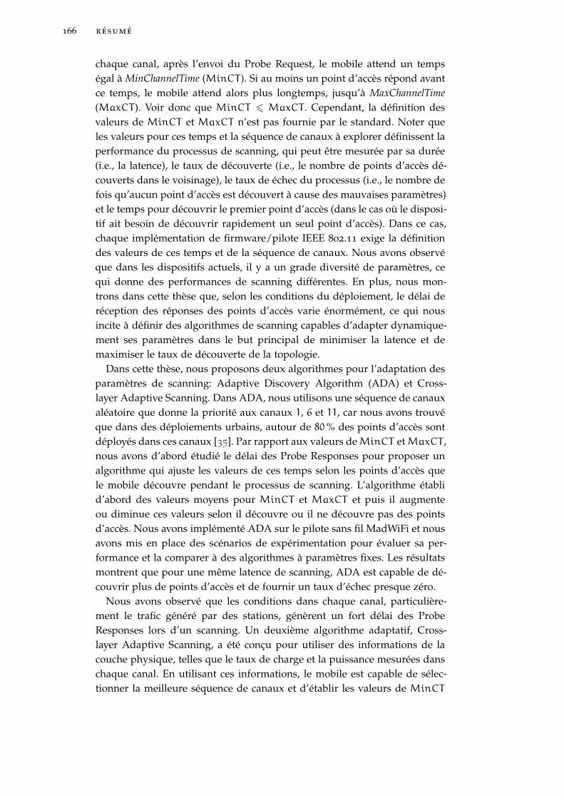
166 résumé

chaque canal, après l’envoi du Probe Request, le mobile attend un tempségal à MinChannelTime (MinCT ). Si au moins un point d’accès répond avantce temps, le mobile attend alors plus longtemps, jusqu’à MaxChannelTime

(MaxCT ). Voir donc que MinCT 6 MaxCT . Cependant, la définition desvaleurs de MinCT et MaxCT n’est pas fournie par le standard. Noter queles valeurs pour ces temps et la séquence de canaux à explorer définissent laperformance du processus de scanning, qui peut être mesurée par sa durée(i.e., la latence), le taux de découverte (i.e., le nombre de points d’accès dé-couverts dans le voisinage), le taux de échec du processus (i.e., le nombre defois qu’aucun point d’accès est découvert à cause des mauvaises paramètres)et le temps pour découvrir le premier point d’accès (dans le cas où le disposi-tif ait besoin de découvrir rapidement un seul point d’accès). Dans ce cas,chaque implémentation de firmware/pilote IEEE 802.11 exige la définitiondes valeurs de ces temps et de la séquence de canaux. Nous avons observéque dans les dispositifs actuels, il y a un grade diversité de paramètres, cequi donne des performances de scanning différentes. En plus, nous mon-trons dans cette thèse que, selon les conditions du déploiement, le délai deréception des réponses des points d’accès varie énormément, ce qui nousincite à définir des algorithmes de scanning capables d’adapter dynamique-ment ses paramètres dans le but principal de minimiser la latence et demaximiser le taux de découverte de la topologie.

Dans cette thèse, nous proposons deux algorithmes pour l’adaptation desparamètres de scanning: Adaptive Discovery Algorithm (ADA) et Cross-layer Adaptive Scanning. Dans ADA, nous utilisons une séquence de canauxaléatoire que donne la priorité aux canaux 1, 6 et 11, car nous avons trouvéque dans des déploiements urbains, autour de 80 % des points d’accès sontdéployés dans ces canaux [35]. Par rapport aux valeurs de MinCT et MaxCT ,nous avons d’abord étudié le délai des Probe Responses pour proposer unalgorithme qui ajuste les valeurs de ces temps selon les points d’accès quele mobile découvre pendant le processus de scanning. L’algorithme établid’abord des valeurs moyens pour MinCT et MaxCT et puis il augmenteou diminue ces valeurs selon il découvre ou il ne découvre pas des pointsd’accès. Nous avons implémenté ADA sur le pilote sans fil MadWiFi et nousavons mis en place des scénarios de expérimentation pour évaluer sa per-formance et la comparer à des algorithmes à paramètres fixes. Les résultatsmontrent que pour une même latence de scanning, ADA est capable de dé-couvrir plus de points d’accès et de fournir un taux d’échec presque zéro.

Nous avons observé que les conditions dans chaque canal, particulière-ment le trafic généré par des stations, génèrent un fort délai des ProbeResponses lors d’un scanning. Un deuxième algorithme adaptatif, Cross-layer Adaptive Scanning, a été conçu pour utiliser des informations de lacouche physique, telles que le taux de charge et la puissance mesurées danschaque canal. En utilisant ces informations, le mobile est capable de sélec-tionner la meilleure séquence de canaux et d’établir les valeurs de MinCT

résumé 167

et MaXCT les plus appropriées pour recevoir les réponses dans chaque scé-nario. Dans ce cas, nous implémentons l’algorithme dans le driver ath5kpour Linux et nous expérimentons dans cinq scénarios de déploiement dif-férents, pour comparer la performance de l’algorithme adaptatif face à desstratégies de paramètres fixes. Nous observons dans ce cas qu’en utilisantdes informations de la couche physique, l’algorithme adaptatif peut iden-tifier des canaux qui ont très probablement des points d’accès déployés etutiliser des temps d’attente plus longues dans ces cas pour augmenter laprobabilité de recevoir des réponses.

Mécanisme de prise de décision pour les terminaux multi-domiciliés

Tel que nous avons montré dans l’étude d’évaluation de la diversité des dé-ploiements sans fil, il existe actuellement un potentiel pour une utilisationsimultanée des interfaces réseaux. Pour cela, l’utilisateur doit définir desmécanismes de sélection des réseaux visant à exploiter la diversité des inter-faces. Typiquement, ils existent deux types de mécanismes pour la sélectiondes réseaux, ceux orientés à déterminer le meilleur réseau pour basculertous les flux d’application (i.e., le cas du handover vertical) et ceux orientéstrouver la répartition des flux la plus optimal entre les différentes interfacesréseaux (i.e., le cas de la multi-domiciliation). Des différentes solutions ontété proposées dans la littérature qui définissent des mécanismes de décisionpour le handover vertical. Ces solutions peuvent être basés sur des algo-rithmes de prise de décision multicritères (MADM) en utilisant des critèrestrès divers (e.g., QoS, profil des utilisateurs, état des interfaces) ou sur desmécanismes de décisions modelés comme des problèmes d’optimisation multi-objectifs. Cependant, dans ces solutions, les problèmes sont suivant sim-plifiés en utilisant des informations de haut niveau visant à établir despréférences des différents critères/objectifs lors de la prise de décision. Cesinformations de haut niveau sont traduites par des poids, qui indiquent unemesure subjective de la préférence. L’utilisation des poids réduit la complex-ité du problème à une seule dimension et empêche à l’utilisateur d’évaluerle compromis qui existe entre des différents critères/objectifs contradictoires.Nous observons aussi que dans les solutions existantes, un nombre très im-portant de critères est utilisé pour la prise de décision, ce qui augmentela complexité du mécanisme car dans ce cas, le dispositif doit surveillerplusieurs paramètres au même temps.

En particulier, la consommation énergétique est parfois considérée commeun critère pour la prise de décision. Typiquement un coût énergétique con-stant est attribué à chaque interface réseaux. Cependant, la consommationd’une interface dépend fortement de la façon dans laquelle elle est utilisée,i.e., des caractéristiques des flux applicatifs transportés par chaque interface.

Nous proposons un mécanisme de sélection des réseaux visant à attribuerles différents flux sur des interfaces disponibles. Nous modélisons ce mé-

168 résumé

canisme comme un problème d’optimisation multi-objectifs qui considèredeux aspects: l’énergie consommée par les interfaces et l’écart entre la de-mande de bande passante des applications et la capacité disponible des inter-faces. D’autre part, pour éviter la subjectivité dans la prise de décision, nousn’utilisons aucun poids pour les objectifs mais des algorithmes génétiquescapables d’obtenir des solutions optimales en évaluant chaque solution surplusieurs objectifs au même temps grâce au critère de non-dominance.

Nous évaluons notre approche par simulation (en utilisant le frameworkpour optimisation multi-objectifs PISA [65]) et nous faisons des compara-isons face à des mécanismes de combinaison de poids type MADM (telsque Simple Additive Weighting ou Multiplicative Exponential Weighting).Nous observons qu’en utilisant des algorithmes génétiques, il est possibled’obtenir plusieurs solutions optimales qui mettent en évidence le compro-mis existant entre les deux objectifs proposés. Nous observons aussi dansnos résultats de simulation que pour les problèmes qui concernent plusieursapplications à attribuer, notre approche permet d’obtenir des solutions plusrapidement qu’en faisant une recherche complète avec des algorithmes baséssur des poids, avec une bonne approximation aux solutions optimales.

conclusion

L’environnement sans fil actuel se caractérise par une diversité de technolo-gies. Ces technologies ont été déployées dans les dernières années visant àfournir un accès Internet sans fil à haut débit pour les utilisateurs mobiles.En particulier dans ces dernières années, les réseaux communautaires baséssur IEEE 802.11 ont été déployés par des abonnes résidentielles ADSL, encréant des réseaux omniprésentes en milieu urbain. Cela ouvre la possibilitéaux utilisateurs multi-domiciliés d’exploiter la diversité des réseaux d’unefaçon « Always Best Connected ».

Toutefois, dans un tel environnement hétérogène sans fil, il y a encorequelques limitations qui empêchent les utilisateurs mobiles d’exploiter pleine-ment la diversité des réseaux. Tout d’abord, comme nous l’avons montrédans l’étude d’évaluation de la diversité des réseaux réalisé avec la plate-forme Wi2Me, même s’il y a une forte densité des réseaux sans fil (IEEE802.11 et les réseaux cellulaires) dans les zones urbaines, la faible intégra-tion des déploiements des différentes technologies empêche les opérateursde fournir une mobilité transparente à travers les différentes technologiesréseau, et plus particulièrement entre les différents points d’accès IEEE 802.11

des différents opérateurs. D’autre part, nous avons également montré dansnotre étude d’évaluation qu’il existe une grande complémentarité des réseauxIEEE 802.11 et les réseaux cellulaires dans le milieu urbain, permettant àl’utilisateur mobile de communiquer avec plusieurs interfaces sans fil à toutmoment. Cependant, il existe actuellement un manque de mécanisme desélection des réseaux pour permettre l’utilisation simultanée de plusieurs in-

résumé 169

terfaces (généralement WLAN et les réseaux cellulaires), afin de maximiserl’exploitation de la diversité sans fil.

Dans cette thèse, nous nous sommes concentrés sur les deux limitationsmentionnées ci-dessus. Après avoir fourni une étude d’évaluation des réseauxsans fil actuels dans les zons urbaines nous avons d’abord analysé les lim-itations de la mobilité et, en particulier, le processus de découverte dansla norme IEEE 802.11. Nous avons montré que les optimisations actuellesde l’algorithme de scanning actif dans IEEE 802.11 ne considèrent pas lecompromis entre la latence du processus et les points d’accès découvertsdans la topologie. Nous gérons ce compromis en proposant un ensembled’algorithmes de scanning adaptatifs, qui visent à définir les paramètresles plus appropriés pour chaque canal. Nous avons implémenté deux algo-rithmes adaptatifs sur des pilotes open-source IEEE 802.11 et nous avons pro-posé une évaluation expérimentale dans deux bancs d’essai différents, afinde comparer les algorithmes adaptatifs contre des algorithmes à paramètresfixes. Les résultats montrent que l’utilisation d’une stratégie d’adaptationpermet de mieux gérer le compromis entre la latence et la découverte detopologie, c’est à dire, pour une latence donnée, un algorithme adaptatif estcapable de découvrir un plus grand nombre de points d’accès.

La deuxième contribution de cette thèse a porté sur le processus de prisede décision pour la sélection des réseaux dans un contexte multi-domicilié.Dans ce cas, nous considérons qu’un utilisateur mobile doit décider com-ment attribuer les flux applicatifs différents pour les interfaces disponibles.Cela diffère des mécanismes existants de sélection des réseaux, qui se con-centrent principalement sur le soutien à la prise de décision pour handoververtical, afin d’optimiser un ensemble de critères (par exemple, la qualitéde service, le coût, la sécurité, l’énergie). Nous considérons particulièrementla consommation d’énergie des interfaces sans fil comme un critère pourla prise de décision. A différence des mécanismes de sélection des réseauxexistants, dans lesquels l’énergie est considérée comme un coût fixe asso-cié à chaque interface, nous prenons en compte la consommation d’énergied’une manière fine. Dans ce cas, nous utilisons des modèles de trafic pourestimer la quantité d’énergie consommée par l’assignation d’un flux surune interface. Nous modélisons le problème d’assignation des flux commeun problème d’optimisation multi-objectif et nous cherchons des solutionsen utilisant des algorithmes génétiques. En tant qu’objectifs, nous consid-érons la minimisation de la consommation d’énergie des interfaces et del’insatisfaction de bande passante qui est généré lorsque la bande passantedemandée par les applications dépasse la bande passante disponible desinterfaces. Nous évaluons notre mécanisme par simulation, en prenant encompte des différents scénarios qui correspondent à des différents typesd’applications et de caractéristiques des interfaces. Les résultats des simu-lations montrent que la résolution du problème avec des algorithmes géné-

170 résumé

tiques fournissent une vue complète du compromis entre les différents ob-jectifs.

Il y a encore un certain nombre de questions ouvertes dans le contexte dela mobilité et de la gestion de la multi-domiciliation dans les réseaux sans filhétérogènes. Même si nous pouvons assurer une latence de handover faibleet une assignation optimale des applications, nous avons observé que dansles dispositifs actuels, il y a encore des limitations qui dégradent l’expériencedes utilisateurs. Tout d’abord, les dispositifs mobiles utilisent généralementune seule interface réseaux à la fois. Toutefois, cette limitation peut être sim-plement remédié en modifiant les politiques implémentés dans le systèmed’exploitation et en mettant en œuvre un protocole de multi-domiciliation(shim6, HIP). Deuxièmement, nous avons constaté que les dispositifs actuelsne sont pas réactifs aux changements dans l’environnement sans fil, c’està dire qu’il n’y a pas des algorithmes de déclenchement intelligents afinde déterminer si la situation actuelle se dégrade et que le dispositif a doncbesoin de s’adapter à cette nouvelle situation. Dans ce cas, le mobile doitdécouvrir des nouveaux réseaux et calculer l’attribution des flux las plusoptimal. Nous travaillons actuellement dans un algorithme d’anticipationsur Android qui surveille l’évolution à court terme du signal avec le pointd’accès pour déclencher le processus adaptatif de découverte (comme ceuxque nous avons proposé dans cette thèse). En ce qui concerne la sélectiondes réseaux, nous avons évalué les processus de décision déclenchés parl’utilisateur (par exemple, lorsque des nouvelles applications sont exécutées).Dans ce cas, nous n’avons pas considéré ce processus étant déclenchée parune modification de l’environnement sans fil. Dans le futur, cette situationpourrait être considérée afin de concevoir des déclencheurs plus efficacespour le processus de prise de décision.

P U B L I C AT I O N S

peer-reviewed journals

1. German Castignani, Alberto Blanc, Alejandro Lampropulos and Nico-las Montavont, Urban 802.11 community networks for mobile users: Cur-

rent deployments and prospectives, Mobile Networks and Applications(MONET), Special Issue on Mobility and Social Networks Confluence,ISSN 1383-469X, pp. 1-12, ACM/Springer, 2012.

2. German Castignani, Andrés Arcia, and Nicolas Montavont, A study

of the discovery process in 802.11 networks. SIGMOBILE Mob. Comput.Commun. Rev. 15, 1, pp. 25-36, March 2011.

peer-reviewed conferences and workshops

3. Yves Josse, Bruno Fracasso, German Castignani and Nicolas Montavont,Energy Efficient Distributed Antenna Systems Deployments using Radio-

over-Fiber, Online Conference on Green Communications (GreenCom),IEEE, 2012

4. German Castignani, Pablo Negri and Nicolas Montavont, Relevamiento

de despliegues de redes IEEE 802.11: Hacia redes inalambricas comunitarias,41◦ Jornadas Argentinas de Informática (JAIIO), Argentina, 2012

5. Laudin Molina, Andrés Arcia-Moret, German Castignani and NicolasMontavont, Caracterización de Topologías Espontáneas IEEE 802.11: Hacia

un Sistema de Redes Comunitarias, 5◦ Congreso Ibero-americano de Estu-diantes de Ingeniería Eléctrica (CIBELEC), Venezuela, 2012

6. German Castignani, Alejandro Lampropulos, Alberto Blanc and Nico-las Montavont, Wi2Me: A Mobile Sensing Platform for Wireless Heteroge-

neous Networks, 32th International Conference on Distributed Comput-ing Systems Workshops (ICDCSW), 2012

7. German Castignani, Nicolas Montavont and Alejandro Lampropulos,Energy considerations for a wireless multi-homed environment, in Energy-Aware Communications (R. Lehnert, ed.), vol. 6955 of Lecture Notesin Computer Science, 17th Eunice Open European Summer School, pp.181-192, Springer Berlin, 2011

8. German Castignani, Nicolas Montavont, Andrés Arcia-Moret, MohamedOularbi and Sebastien Houcke, Cross-layer adaptive scanning algorithms

171

172 publications

for IEEE 802.11 networks, Wireless Communications and NetworkingConference (WCNC), IEEE, pp. 327-332, March 2011

9. German Castignani, Lucien Loiseau and Nicolas Montavont, An evalu-

ation of IEEE 802.11 community networks deployments, Information Net-working (ICOIN), 2011 International Conference on, pp.498-503, 2011

10. German Castignani, Andrés Arcia-Moret and Nicolas Montavont, An

evaluation of the resource discovery process in IEEE 802.11 networks, In Pro-ceedings of the Second International Workshop on Mobile Opportunis-tic Networking (MobiOpp ’10), ACM, 2010

11. German Castignani, Andrés Arcia-Moret and Nicolas Montavont, Anal-

ysis and Evaluation of WiFi Scanning Strategies, 4◦ Congreso Iberoamer-icano de Estudiantes de Ingeniería Eléctrica (CIBELEC), Venezuela,2010

12. German Castignani and Nicolas Montavont, Adaptive System for 802.11

Scanning, INFOCOM Workshops 2009, IEEE, pp. 1-2, April 2009

13. German Castignani and Nicolas Montavont, Adaptive discovery mech-

anism for wireless environments, 14th Eunice Open European SummerSchool, 2008

internal research reports

14. German Castignani, Nicolas Montavont, Andrés Arcia-Moret, MohamedOularbi and Sebastien Houcke, IEEE 802.11 scanning algorithms: cross-

layer experiments, Collection des rapports de re-cherche de TELECOMBretagne, RR-2011-05-RSM, ISSN 1255-2275, 2011

A C R O N Y M S

2G Second Generation Wireless Network

3GPP 3rd Generation Partnership Project

3G Third Generation Wireless Network

4G Fourth Generation Wireless Network

AAA Authentication, Authorization and Accounting

ABC Always Best Connected

ACO Ant Colony Optimization

ADA Adaptive Discovery Algorithm

ADSL Asymmetric Digital Subscriber Line

AHP Analytic Hierarchy Process

AMVHO Adaptive Multi-Criteria Vertical Handover

ANN Artificial Neural Networks

AP Access Point

BBV Bi-objective Binary Value

BER Bit Error Rate

BSSID Basic Service Set Identifier

BSS Basic Service Set

CCK Complementary Code Keying

CDF Cumulative Distribution Function

CDMA Code Division Multiple Access

CGI Common Gateway Interface

CID Cell Identifier

CN Community Networks

CSMA/CA Carrier Sense Multiple Access with Collision Avoidance

CWND TCP Congestion Window

DCF Distributed Coordination Function

173

174 acronyms

DCH Dedicated Channel

DHCP Dynamic Host Configuration Protocol

DIFS DCF Interframe Space

DSSS Direct Sequence Spread Spectrum

DS Distribution System

E-DCH Enhanced Dedicated Channel

EAP Extensible Authentication Protocol

EAP-SIM Extensible Authentication Protocol Method for GSM SubscriberIdentity Module

EDGE Enhanced Data Rates for GSM Evolution

ESS Extended Service Set

FACH Forward Access Channel

FDD Frequency-Division Duplexing

FEMO Fair Evolutionary Multiobjective Optimizer

FHSS Frequency Hopping Spread Spectrum

FIS Fuzzy Inference System

FRD First Probe Response Delay

GPRS General Packet Radio Service

GPS Global Positioning System

GRA Grey Relational Analysis

GRC Grey Relational Coefficient

GSM Global System for Mobile Communications

HIP Host Identity Protocol

HSDPA High Speed Downlink Packet Access

HSPA+ Evolved High Speed Packet Access

HSPA High Speed Packet Access

HSUPA High Speed Uplink Packet Access

HTTPS Hypertext Transfer Protocol Secure

IBSS Independent Basic Service Set

acronyms 175

IFS Interframe-Spacing

ISM Industrial Scientific and Medical

ISP Internet Service Provider

IoT Internet of Things

LAC Location Area Code

LMS Least Mean Square

LMPA Local Maximum Precision Algorithm

LOTZ Leading Ones Trailing Zeros

LTE Long Term Evolution

MAC Medium Access Control

MADM Multi-Attribute Decision Making

MEW Multiplicative Exponential Weighting

MIMO Multiple Input Multiple Output

MOO Multi-Objective Optimization

MS Mobile Station

MVC Model View Controller

MoS Mean Opinion Score

NAT Network Address Translation

NSGA2 Non-dominated Sorting Genetic Algorithm 2

NSGA Non-dominated Sorting Genetic Algorithm

OFDMA Orthogonal Frequency-Division Multiple Access

OFDM Orthogonal Frequency Division Multiplexing

OS Operative Systems

PCH Paging Channel

PERL Practical Extraction and Report Language

PSM Power Saving Mode

QoS Quality of Service

RADIUS Remote Authentication Dial-In User Service

RNC Radio Network Controller

176 acronyms

RRC Radio Resource Control

RSSI Received Signal Strength Indication

RTT Round Trip Time

RWND TCP Receiver Window

SAW Simple Additive Weighting

SIM Subscriber Identity Modules

SPA Simple Precision Algorithm

SPEA2 Strength Pareto Evolutionary Algorithm 2

SSID Service Set Identifier

TDD Time-Division Duplexing

TDMA Time Division Multiple Access

TIM Traffic Indication Map

TOPSIS Technique for Order Preference by Similarity to Ideal Solution

TU Time Unit

UMTS Universal Mobile Telecommunications System

USRP2 Universal Software Radio Peripheral

VoIP Voice over Internet Protocol

VPN Virtual Private Network

WCDMA Wideband Code Division Multiple Access

WEP Wired Equivalent Privacy

WLAN Wireless Local Area Networks

WPAN Wireless Personal Area Networks

WPA Wi-Fi Protected Access

WSN Wireless Sensor Networks

WiMAX Worldwide Interoperability for Microwave Access

Exploiting Network Diversity - Archives-Ouvertes.fr

Documents

Transcript of Exploiting Network Diversity - Archives-Ouvertes.fr