STATISTICS IN MEDICINEStatist. Med. 2003; 22:2503–2513 (DOI: 10.1002/sim.1464)

Assessment of diagnostic markers by goodness-of-�t tests

Christos Nakas1, Constantin T. Yiannoutsos2;∗, Ronald J. Bosch3 andChronis Moyssiadis1

1Department of Mathematics; Statistics and OR Unit; Aristotle University; 54006 Thessaloniki; Greece2 Indiana University Cancer Center; 535 Barnhill Drive; RT 380H; Indianapolis; IN 46202; U.S.A.

3Department of Biostatistics; Harvard University; 651 Huntington Avenue; Boston; MA 02115; U.S.A.

SUMMARY

Receiver operating characteristic (ROC) curves are useful statistical tools used to assess the precisionof diagnostic markers or to compare new diagnostic markers with old ones. The most common indexemployed for these purposes is the area under the ROC curve (�) and several statistical tests existthat test the null hypotheses H0 : �=0:5 or H0 : �1 = �2, in the case of two-marker comparisons, againstalternatives of interest. In this paper we show that goodness-of-�t of uniformity of the distribution ofthe false positive (true positive) rates can be used instead of tests based on the area index. A semi-parametric approach is based on a completely speci�ed distribution of marker measurements for eitherthe healthy (F) or diseased (G) subjects, and this is extended to the two-marker case. We then extendto the one- and two-marker case when neither distribution is speci�ed (the non-parametric case). Ingeneral, ROC-based tests are more powerful than goodness-of-�t tests for location di�erences betweenthe distributions of healthy and diseased subjects. However ROC-based tests are less powerful whenlocation-scale di�erences exist (producing ROC curves that cross the diagonal) and are incapable ofdiscriminating between healthy and diseased samples when �=0:5 but F �=G. In these cases, goodness-of-�t tests have a distinct advantage over ROC-based tests. In conclusion, ROC methodology shouldbe used with recognition of its potential limitations and should be replaced by goodness-of-�t testswhen appropriate. The latter are a viable alternative and can be used as a ‘black box’ or as an ex-ploratory �rst step in the evaluation of novel diagnostic markers. Copyright ? 2003 John Wiley &Sons, Ltd.

KEY WORDS: receiver operating characteristic; ROC; area under the curve; goodness-of-�t

1. INTRODUCTION

In medical research, assessment of a diagnostic marker’s ability to discriminate betweenhealthy and diseased subjects is routinely performed by use of receiver operating

∗Correspondence to: Constantin T. Yiannoutsos, Indiana University Cancer Center, 535 Barnhill Drive, RT 380H,Indianapolis, IN 46202, U.S.A.

Contract=grant sponsor: NIH; contract=grant number: MH-60565.

Received March 2002Copyright ? 2003 John Wiley & Sons, Ltd. Accepted October 2002

2504 C. NAKAS ET AL.

characteristic (ROC) curves. The ROC curve is a plot of the true positive rates (TP) againstfalse positive rates (FP), (or equivalently of the sensitivity against 1-speci�city rate), as acut-o� point is varied along the axis of real numbers.Let X1; X2; : : : ; Xn i.i.d. with continuous distribution function F , be n measurements on

healthy subjects and Y1; Y2; : : : ; Ym i.i.d. with continuous distribution function G, be m measure-ments on diseased subjects. For application of the ROC methodology suppose that diseasedsubjects tend to have higher measurements than healthy subjects. The ROC curve is de�nedas 1−G(F−1(1− p)), 06p61. The area under the curve, denoted here by �, is commonlyused as an overall performance index of a single diagnostic marker, or for the comparisonof two or more diagnostic markers. The idea is that the marker with larger true-positive thanfalse-positive rates at each cutpoint (and thus higher �) better discriminates between diseasedand healthy subjects. In this respect, � is an index of the overlap of F and G. It varies from0.5, when the marker measurement distributions of healthy and diseased subjects completelyoverlap, to 1, when there is no overlap at all.It has been shown [1] that �=Pr(X¡Y ) when the measurements are made on a continuous

scale. Formal statistical tests [2–11] have been proposed to test the null hypothesis H0 : �=0:5.Using Fn and Gm, the empirical distribution function (EDF) estimates of F and G, respectively,the ROC curve is constructed by connecting points (1 − Fn(ci); 1 − Gm(ci)), for a choice ofk cut-o� values, c1; c2; : : : ; ck over the line of real numbers. In that case, � calculated bythe trapezoidal rule is equivalent to the Mann–Whitney statistic [1] and the signi�cance ofthe diagnostic marker is commonly tested based on this proposition. In the semi-parametriccase, that is, when one of the distributions is known, ROC curves have been studied byLi et al. [7].When the marker distribution among healthy (or diseased) subjects is completely speci-

�ed, if the ROC curve is constructed using the marker measurements on diseased (healthy)subjects as cutpoints, a well-known statistical property reveals the intimate relationship be-tween ROC curves and of goodness-of-�t tests in assessing the performance of a diagnosticmarker. In the next section, we show that in the single-marker case, testing that the sampleof FP (or of TP) follows a uniform distribution over (0; 1) is in turn equivalent to testingH0 :F =G when the distribution of healthy (diseased) subjects is known. This null hypothe-sis implies H0 : �=0:5. We extend the goodness-of-�t approach to comparing two diagnosticmarkers.In the more practically relevant situation when neither distribution is speci�ed (‘non-

parametric’ situation), we extend the goodness-of-�t methodology along similar lines as inthe semi-parametric case. The same ideas apply, but appeal to asymptotic distributions of thesingle-sample goodness-of-�t test statistics is inappropriate so Monte Carlo methods must beused to determine critical values for their distribution for the samples that usually arise inpractice.This paper is organized as follows. In Section 2 the use of goodness-of-�t tests for the val-

idation of diagnostic procedures is motivated and the relevant theory is outlined. In Section 3,a series of simulations has been carried out to compare the statistical power of goodness-of-�t tests versus tests based on the area under the ROC curve. Both the semi-parametric andnon-parametric cases are considered in single- and two-marker comparisons. In case, the mostcommon ROC-based test is used as the benchmark. In Section 4 these procedures are appliedto data concerning T-lymphocyte subsets as diagnostic markers of brucellosis. The paper iscompleted by a discussion in Section 5.

Copyright ? 2003 John Wiley & Sons, Ltd. Statist. Med. 2003; 22:2503–2513

GOODNESS-OF-FIT TESTING OF DIAGNOSTIC MARKERS 2505

2. METHODS

2.1. Semi-parametric assessment of diagnostic markers

To develop the goodness-of-�t approach suppose that the distribution of healthy subjects isfully speci�ed for a diagnostic marker and measurements Y1; Y2; : : : ; Ym on diseased subjectsare available. An ROC curve can be constructed by connecting the TP versus FP pointsfor a choice of cut-o� points c1; c2; : : : ; ck . For the ith cut-o� point, FPi=1 − F(ci) andTPi=

(#(Yj)¿ ci)m =1 − Gm(ci), for j=1; : : : ; k. Assessment of a single diagnostic marker can

be based either on asymptotic normality of � [7], or by constructing Monte Carlo con�denceintervals for � [7, 12].A possible choice of cut-o� points, in the case when F is completely speci�ed, are the

measurements on the diseased subjects Y1; Y2; : : : ; Ym (the measurements of the healthy subjectswould be considered if G were speci�ed and F were not). To construct this version of theROC curve, we calculate the FP and TP rates by considering ci=Yi, i=1; : : : ; m:

FPi=1− F(Yi) and TPi=1−Gm(Yi); i=1; : : : ; m

It is well known that by the probability integral transformation (for example, reference [13])

U1 =G(Y1); U2 =G(Y2); : : : ; Um=G(Ym) are i:i:d: U(0; 1)

and thus so are 1 − Ui; i=1; : : : ; m. Thus if F =G (the area under the ROC curve de�nedby F;G equals 0:5 [3]), then

V1 =F(Y1); V2 =F(Y2); : : : ; Vm=F(Ym) are i:i:d: U(0; 1)

and thus so will 1− Vi; i=1; : : : ; m (that is, the FPi).It is easily seen that testing the hypothesis H0 :F =G is equivalent to testing that the

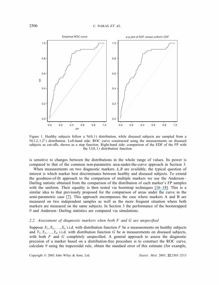
distribution H (x)=G◦F−1(x) is equal to a uniform distribution on (0; 1). The null hypothesisof equality of F and G (and thus of the equality of H to a uniform) implies the null hypothesisH0 : �=0:5 (the reverse is not always true). The uniformity of H can be tested by a p−p plotof the FPi ; i=1; : : : ; m (that is, 1 − Vi above) versus the quantiles of a uniform distributionon (0; 1). The ROC curve constructed by using the observations of the diseased subjects ascut-o� points is the same as the p−p plot of the empirical distribution function of FP againstthe uniform distribution on (0; 1).Figure 1 shows the ROC curve comparing 50 random measurements from N(0; 1) versus

50 measurements from N(1:2; 1:22) (plot on the left). This is the same as the p − p plot ofthe empirical distribution function of FP against the uniform on (0; 1) (plot on the right).This duality of p− p plots and ROC curves has been well documented [7, 14]. It re�ects

the nature of the diagnostic-testing problem as one of measuring the degree of di�erentiationbetween the distributions of diagnostic-marker measurements obtained on healthy and diseasedindividuals. Useful diagnostic markers are those that result in a ‘signi�cant’ di�erentiationbetween the distributions of the marker measurements among healthy and diseased subjectsaccording to some criterion. The equality of these two distributions can be tested by goodness-of-�t tests. The equivalency between the hypotheses H0 :F =G and H0 :H =U also suggeststhat the latter can be tested instead of the former. We proceed to test the equality of H with auniform distribution. Our choice of test procedure is the Anderson–Darling test [13, 15] which

Copyright ? 2003 John Wiley & Sons, Ltd. Statist. Med. 2003; 22:2503–2513

2506 C. NAKAS ET AL.

0.0 0.2 0.4 0.6 0.8 1.0

FP

1.0

0.8

0.6

0.4

0.2

0.0

1.0

0.8

0.6

0.4

0.2

0.0

TP

Empirical ROC curve

0.0 0.2 0.4 0.6 0.8 1.0

p-p plot of EDF versus uniform CDF

Figure 1. Healthy subjects follow a N(0; 1) distribution, while diseased subjects are sampled from aN(1:2; 1:22) distribution. Left-hand side: ROC curve constructed using the measurements on diseasedsubjects as cut-o�s, shown as a step function. Right-hand side: comparison of the EDF of the FP with

the U(0; 1) distribution function.

is sensitive to changes between the distributions in the whole range of values. Its power iscompared to that of the common non-parametric area-under-the-curve approach in Section 3.When measurements on two diagnostic markers A; B are available, the typical question of

interest is which marker best discriminates between healthy and diseased subjects. To extendthe goodness-of-�t approach to the comparison of multiple markers we use the Anderson–Darling statistic obtained from the comparison of the distribution of each marker’s FP sampleswith the uniform. Their equality is then tested via bootstrap techniques [16–18]. This is asimilar idea to that previously proposed for the comparison of areas under the curve in thesemi-parametric case [7]. This approach encompasses the case where markers A and B aremeasured on two independent samples as well as the more frequent situation where bothmarkers are measured on the same subjects. In Section 3 the performance of the bootstrapped� and Anderson–Darling statistics are compared via simulations.

2.2. Assessment of diagnostic markers when both F and G are unspeci�ed

Suppose X1; X2; : : : ; Xn i.i.d. with distribution function F be n measurements on healthy subjectsand Y1; Y2; : : : ; Ym i.i.d. with distribution function G be m measurements on diseased subjects,with both F and G completely unspeci�ed. A general approach to assess the diagnosticprecision of a marker based on a distribution-free procedure is to construct the ROC curve,calculate � using the trapezoidal rule, obtain the standard error of this estimate (for example,

Copyright ? 2003 John Wiley & Sons, Ltd. Statist. Med. 2003; 22:2503–2513

GOODNESS-OF-FIT TESTING OF DIAGNOSTIC MARKERS 2507

Table I. Quantiles of the Anderson–Darling statistic in the non-parametric case.

Sample size

n=m=30 n=m=50 n=m=100

q0:90 3.395 3.570 3.728q0:95 4.429 4.526 4.784q0:99 7.074 7.497 7.713

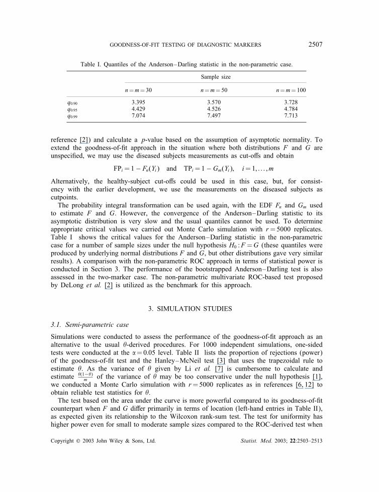
reference [2]) and calculate a p-value based on the assumption of asymptotic normality. Toextend the goodness-of-�t approach in the situation where both distributions F and G areunspeci�ed, we may use the diseased subjects measurements as cut-o�s and obtain

FPi=1− Fn(Yi) and TPi=1−Gm(Yi); i=1; : : : ; m

Alternatively, the healthy-subject cut-o�s could be used in this case, but, for consist-ency with the earlier development, we use the measurements on the diseased subjects ascutpoints.The probability integral transformation can be used again, with the EDF Fn and Gm used

to estimate F and G. However, the convergence of the Anderson–Darling statistic to itsasymptotic distribution is very slow and the usual quantiles cannot be used. To determineappropriate critical values we carried out Monte Carlo simulation with r=5000 replicates.Table I shows the critical values for the Anderson–Darling statistic in the non-parametriccase for a number of sample sizes under the null hypothesis H0 :F =G (these quantiles wereproduced by underlying normal distributions F and G, but other distributions gave very similarresults). A comparison with the non-parametric ROC approach in terms of statistical power isconducted in Section 3. The performance of the bootstrapped Anderson–Darling test is alsoassessed in the two-marker case. The non-parametric multivariate ROC-based test proposedby DeLong et al. [2] is utilized as the benchmark for this approach.

3. SIMULATION STUDIES

3.1. Semi-parametric case

Simulations were conducted to assess the performance of the goodness-of-�t approach as analternative to the usual �-derived procedures. For 1000 independent simulations, one-sidedtests were conducted at the �=0:05 level. Table II lists the proportion of rejections (power)of the goodness-of-�t test and the Hanley–McNeil test [3] that uses the trapezoidal rule toestimate �. As the variance of � given by Li et al. [7] is cumbersome to calculate andestimate �(1−�)

m of the variance of � may be too conservative under the null hypothesis [1],we conducted a Monte Carlo simulation with r=5000 replicates as in references [6, 12] toobtain reliable test statistics for �.The test based on the area under the curve is more powerful compared to its goodness-of-�t

counterpart when F and G di�er primarily in terms of location (left-hand entries in Table II),as expected given its relationship to the Wilcoxon rank-sum test. The test for uniformity hashigher power even for small to moderate sample sizes compared to the ROC-derived test when

Copyright ? 2003 John Wiley & Sons, Ltd. Statist. Med. 2003; 22:2503–2513

2508 C. NAKAS ET AL.

Table II. Power based on 1000 independent simulations in the semi-parametric case∗.

Tests Sample size

m=30 m=50 m=100

� 0.601 0.501 0.853 0.724 0.507 0.939 0.905 0.751 1.000Anderson–Darling 0.361 0.655 0.747 0.550 0.810 0.920 0.823 0.987 0.998

∗ Left-hand entry: F ∼ N(0; 1), Gm ∼ N(0:3; 1), middle entry: F ∼ N(0; 1), Gm ∼ N(0:3; 1:42),right-hand entry: F ∼ Beta(2; 3), Gm ∼ Beta(2; 2).

FP

TP

0.0 0.2 0.4 0.6 0.8 1.0

0.0

0.2

0.4

0.6

0.8

1.0

FP

TP

0.0 0.2 0.4 0.6 0.8 1.0

0.0

0.2

0.4

0.6

0.8

1.0

FP

TP

0.0 0.2 0.4 0.6 0.8 1.0

0.0

0.2

0.4

0.6

0.8

1.0

0.0 0.2 0.4 0.6 0.8 1.0

0.0

0.01

0.02

-5.0 0.0 5.0-2.5 2.5

0.0

0.1

0.2

0.3

0.4

0.0

0.1

0.2

0.3

0.4

-5.0 0.0 5.0-2.5 2.5

Figure 2. Probability distribution functions and their corresponding ROC curves (m= n=100) forthe cases described in Table II N(0; 1) versus N(0:3; 1) (left), N(0; 1) versus N(0:3; 1:42) (centre),

Beta(2; 2) versus Beta(2; 3) (right).

F and G are di�erent primarily in terms of location and shape (middle entries in Table II).This is the case of ROC curves that cross the reference diagonal, which have been consideredin previous studies [19]. The situation is shown graphically in Figure 2.

3.2. Non-parametric case

When the distributions of marker measurements F and G are unspeci�ed, quantiles similarto those of Table I can be used for the comparison of the Anderson–Darling statistic to theordinary non-parametric ROC test at level �=0:05. Results are shown in Table III. Similarlyto the semi-parametric case, the ROC-based test is more powerful than the goodness-of-�t testwhen location di�erences are primarily involved. However, when scale di�erences between

Copyright ? 2003 John Wiley & Sons, Ltd. Statist. Med. 2003; 22:2503–2513

GOODNESS-OF-FIT TESTING OF DIAGNOSTIC MARKERS 2509

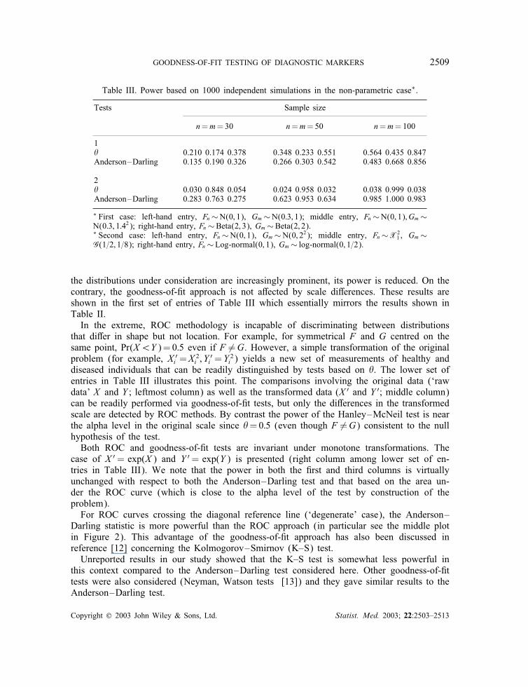
Table III. Power based on 1000 independent simulations in the non-parametric case∗.

Tests Sample size

n=m=30 n=m=50 n=m=100

1� 0.210 0.174 0.378 0.348 0.233 0.551 0.564 0.435 0.847Anderson–Darling 0.135 0.190 0.326 0.266 0.303 0.542 0.483 0.668 0.856

2� 0.030 0.848 0.054 0.024 0.958 0.032 0.038 0.999 0.038Anderson–Darling 0.283 0.763 0.275 0.623 0.953 0.634 0.985 1.000 0.983

∗ First case: left-hand entry, Fn∼N(0; 1), Gm∼N(0:3; 1); middle entry, Fn∼N(0; 1); Gm∼N(0:3; 1:42); right-hand entry, Fn∼Beta(2; 3), Gm∼Beta(2; 2).∗ Second case: left-hand entry, Fn∼N(0; 1), Gm∼N(0; 22); middle entry, Fn∼X2

1 , Gm∼G(1=2; 1=8); right-hand entry, Fn∼Log-normal(0; 1), Gm∼ log-normal(0; 1=2).

the distributions under consideration are increasingly prominent, its power is reduced. On thecontrary, the goodness-of-�t approach is not a�ected by scale di�erences. These results areshown in the �rst set of entries of Table III which essentially mirrors the results shown inTable II.In the extreme, ROC methodology is incapable of discriminating between distributions

that di�er in shape but not location. For example, for symmetrical F and G centred on thesame point, Pr(X¡Y )=0:5 even if F �=G. However, a simple transformation of the originalproblem (for example, X ′

i =X2i ; Y

′i =Y

2i ) yields a new set of measurements of healthy and

diseased individuals that can be readily distinguished by tests based on �. The lower set ofentries in Table III illustrates this point. The comparisons involving the original data (‘rawdata’ X and Y ; leftmost column) as well as the transformed data (X ′ and Y ′; middle column)can be readily performed via goodness-of-�t tests, but only the di�erences in the transformedscale are detected by ROC methods. By contrast the power of the Hanley–McNeil test is nearthe alpha level in the original scale since �=0:5 (even though F �=G) consistent to the nullhypothesis of the test.Both ROC and goodness-of-�t tests are invariant under monotone transformations. The

case of X ′= exp(X ) and Y ′= exp(Y ) is presented (right column among lower set of en-tries in Table III). We note that the power in both the �rst and third columns is virtuallyunchanged with respect to both the Anderson–Darling test and that based on the area un-der the ROC curve (which is close to the alpha level of the test by construction of theproblem).For ROC curves crossing the diagonal reference line (‘degenerate’ case), the Anderson–

Darling statistic is more powerful than the ROC approach (in particular see the middle plotin Figure 2). This advantage of the goodness-of-�t approach has also been discussed inreference [12] concerning the Kolmogorov–Smirnov (K–S) test.Unreported results in our study showed that the K–S test is somewhat less powerful in

this context compared to the Anderson–Darling test considered here. Other goodness-of-�ttests were also considered (Neyman, Watson tests [13]) and they gave similar results to theAnderson–Darling test.

Copyright ? 2003 John Wiley & Sons, Ltd. Statist. Med. 2003; 22:2503–2513

2510 C. NAKAS ET AL.

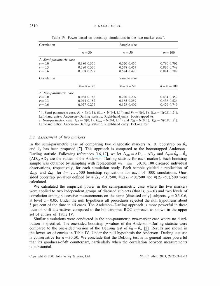
Table IV. Power based on bootstrap simulations in the two-marker case∗.

Correlation Sample size

m=30 m=50 m=100

1. Semi-parametric caser=0:0 0.380 0.350 0.520 0.456 0.790 0.702r=0:3 0.380 0.330 0.538 0.457 0.826 0.748r=0:6 0.308 0.278 0.524 0.420 0.884 0.788

Correlation Sample size

n=m=30 n=m=50 n=m=100

2. Non-parametric caser=0:0 0.088 0.162 0.220 0.207 0.434 0.352r=0:3 0.044 0.182 0.185 0.259 0.438 0.524r=0:6 0.027 0.277 0.128 0.409 0.429 0.749

∗ 1. Semi-parametric case: FA ∼N(0; 1), GmA ∼N(0:4; 1:12) and FB∼N(0; 1), GmB∼N(0:8; 1:22).Left-hand entry: Anderson–Darling statistic. Right-hand entry: bootstrapped �s.2. Non-parametric case: FnA ∼N(0; 1), GmA ∼N(0:4; 1:12) and FnB∼N(0; 1), YmB∼N(0:8; 1:22).Left-hand entry: Anderson–Darling statistic. Right-hand entry: DeLong test.

3.3. Assessment of two markers

In the semi-parametric case of comparing two diagnostic markers A, B, bootstrap on �Aand �B has been proposed [7]. This approach is compared to the bootstrapped Anderson–Darling statistic. Following references [16, 17], we let �AD =ADB − ADA and ��= �̂B − �̂A(ADA;ADB are the values of the Anderson–Darling statistic for each marker). Each bootstrapsample was obtained by sampling with replacement mA =mB =30; 50; 100 diseased individualobservations, respectively, for each simulation study. Each sample yielded a replication of�ADi and ��i , for i=1; : : : ; 500 bootstrap replications for each of 1000 simulations. One-sided bootstrap p-values de�ned by #(�N¡0)=500, #(�AD¡0)=500 and #(��¡0)=500 werecalculated.We calculated the empirical power in the semi-parametric case where the two markers

were applied to two independent groups of diseased subjects (that is, �=0) and two levels ofcorrelation among successive measurements on the same (diseased only) subjects, �=0:3; 0:6,at level �=0:05. Under the null hypothesis all procedures rejected the null hypothesis about5 per cent of the time in all cases. The Anderson–Darling approach is more powerful in theselocation-shift alternatives compared to the bootstrapped ROC approach as shown in the upperset of entries of Table IV.Similar simulations were conducted in the non-parametric two-marker case where no distri-

bution is speci�ed. The one-sided bootstrap p-values of the Anderson–Darling statistic werecompared to the one-sided version of the DeLong test of �B − �A [2]. Results are shown inthe lower set of entries in Table IV. Under the null hypothesis the Anderson–Darling statisticis conservative for n=30; 50. We conclude that the DeLong test is in general more powerfulthan its goodness-of-�t counterpart, particularly when the correlation between measurementsis substantial.

Copyright ? 2003 John Wiley & Sons, Ltd. Statist. Med. 2003; 22:2503–2513

GOODNESS-OF-FIT TESTING OF DIAGNOSTIC MARKERS 2511

4. AN APPLICATION

Brucellosis is an intra-cellular bacterial disease transmitted to humans primarily by contactwith infected animals or by ingestion of unpasteurized dairy products. Defects of the cellularimmunity and T-lymphocytes have been described in brucellosis patients [20]. The aim of ourstudy was to investigate di�erences on the proliferation and the stimulation of T-lymphocytesbetween groups of 35 brucellosis patients and 15 controls. T-lymphocyte subsets (CD3, CD4)were studied from phytohemagglutinin (PHA) cultured peripheral blood.Figure 3 shows the ROC curves obtained for the CD3 and CD4 markers. The areas under

the ROC curves associated with these markers are 0.811 and 0.918, respectively (p¡0:001in both cases). Based on the Anderson–Darling statistic, CD3 and CD4 are both signi�cantindividual predictors of brucellosis (p=0:005, p=0:001, respectively). Both procedures agreeon the signi�cance of the markers in distinguishing individuals infected with brucellosis fromuninfected controls.To determine whether CD3 or CD4 is the most signi�cant marker for the detection of bru-

cellosis, we used the test proposed by DeLong et al. [2] and obtained p=0:109. According tothis test neither marker is signi�cantly superior to the other in terms of detecting brucellosis atthe �=0:05 level. The bootstrap procedure based on the Anderson–Darling statistic producedp=0:492. Since our measurements are highly correlated (�=0:635), reliance on the DeLongtest is advisable in this case. Stimulation of CD4-positive lymphocytes is not signi�cantlysuperior to CD3-positive lymphocytes as a marker for the detection of brucellosis accordingto these tests.

FP

1.00.75.50.250.00

TP

1.00

.75

.50

.25

0.00

Reference Line

CD4 PHA

CD3 PHA

Figure 3. Comparison of the ROC curves of markers CD3 and CD4 for the detection of brucellosis.

Copyright ? 2003 John Wiley & Sons, Ltd. Statist. Med. 2003; 22:2503–2513

2512 C. NAKAS ET AL.

5. DISCUSSION

Various choices of cutpoints have been proposed in the analysis of ROC curves arising inthe assessment of a diagnostic marker or test. The area under the curve can vary signi�-cantly with the choice of the cut-o� points. Algorithms estimating the ROC curve based onthe binormality assumption converge to cut-o�s that maximize the area under the curve [5].An alternative is the use of goodness-of-�t tests assessing the equality of the marker mea-surements among healthy and diseased individuals. The hypothesis of equality F =G can bereduced to the comparison of H =G◦F−1 with a uniform distribution on (0; 1). When the dis-tribution of healthy (diseased) subject measurements is known, this goodness-of-�t approachcorresponds to specifying an ROC curve with the diseased-subject (healthy-subject) observa-tions as cut-o�s. We chose the Anderson–Darling test as representative of the goodness-of-�tapproach. Other methods, such as the Kolmogorov–Smirnov Neyman and Watson tests werealso considered (results not shown) but they generally produced slightly lower power thanthe Anderson–Darling test.Assessing the di�erences of the distributions F and G by goodness-of-�t methods produces

consistently high power even in cases where ROC-based tests fail. A case in point concernsshape di�erences between F and G. Tests of H0 :F =G by the ROC approach are useful forlocation alternatives but are less capable of discriminating between distributions that di�er interms of shape and location. In the extreme case of symmetric F and G that di�er only interms of scale, � will be close to 0.5. This eliminates a number of potentially useful testsfrom consideration by ROC methodology even in cases where F is much di�erent from G.One could argue that only location di�erences are diagnostic in practice. However a simpletransformation of the data (for example, a square or absolute-value transformation) will yielda new marker that is diagnostic in the traditional sense. Such markers could otherwise bemissed by solely relying on criteria based on the area under the ROC curve. By contrast,goodness-of-�t tests have adequate power to discriminate between distributions of diseasedand healthy subjects in both the original and the transformed scale. An example of this waspresented in Table III for the case of the square transformation (last-column entry).An attractive property of ROC curves is their invariance under monotone transformations.

This is shared by goodness-of-�t tests as shown in Table III for the exponential transforma-tion. The simulated powers are virtually identical across the �rst and second columns (un-transformed and transformed scale, respectively) for all tests, although, by the construction ofthe problem, the power of the ROC-derived test is near the alpha level. By comparison, thegoodness-of-�t tests exhibit much higher power in discriminating between the two distribu-tions and are thus an attractive alternative to ROC-based methodology and indeed constitutein many cases an improvement over these methods.The Kolmogorov–Smirnov and Anderson–Darling statistics are closely connected to max-

imally selected chi-square statistics. Their relationship with diagnostic testing has long beenrecognized [21, 22]. The Anderson–Darling statistic is also related to the Neyman test [23].The Neyman and Anderson–Darling tests can thus be interpreted as adjusted measures ofmaximum separation of diagnostic marker distributions of healthy and diseased subjects, withthe adjustment made over all quantiles 0¡p¡1.Bloch [16] extends the utility of a similar statistic as that investigated by Gail and Green [21]

in the case of the comparison of two diagnostic markers against the same ‘gold standard’ in asingle sample. His methods are similar to ours in terms of implementing a bootstrap approach

Copyright ? 2003 John Wiley & Sons, Ltd. Statist. Med. 2003; 22:2503–2513

GOODNESS-OF-FIT TESTING OF DIAGNOSTIC MARKERS 2513

for derivation of the distribution of the di�erence of the individual statistics associated with thetwo diagnostic markers. In our case, using bootstrap methods to combine two goodness-of-�tstatistics produced comparable results compared with the non-parametric test of DeLong et al.[2], suggesting that the goodness-of-�t approach can be viably utilized in comparisons of twodiagnostic markers as well.

ACKNOWLEDGEMENTS

The authors extend their gratitude to Dr Evaggelia Zacharioudaki for supplying the brucellosis data.Dr Yiannoutsos’ research was partially supported by NIH grant MH-60565.

REFERENCES

1. Bamber D. The area above the ordinal dominance graph and the area below the receiver operating characteristicgraph. Journal of Mathematical Psychology 1975; 12:387–415.

2. DeLong ER, DeLong DM, Clarke-Pearson DL. Comparing the areas under two or more correlated receiveroperating characteristic curves: a non-parametric approach. Biometrics 1988; 44:837–845.

3. Hanley JA, McNeil BJ. The meaning and use of the area under a receiver operating characteristic (ROC) curve.Radiology 1982; 143:29–36.

4. Hanley JA, McNeil BJ. A method for comparing the areas under receiver operating characteristic curves derivedfrom the same cases. Radiology 1983; 148:839–843.

5. Hsieh F, Turnbull BW. Non-parametric and semi-parametric estimation of the receiver operating characteristiccurve. Annals of Statistics 1996; 24:25–40.

6. Jensen K, M�uller HH, Sch�a�er H. Regional con�dence bands for ROC curves. Statistics in Medicine 2000;19:493–509.

7. Li G, Tiwari RC, Wells MT. Semi-parametric inference for a quantile comparison function with applications toreceiver operating characteristic curves. Biometrika 1999; 86:487–502.

8. Ma G, Hall WJ. Con�dence bands for receiver operating characteristic curves. Medical Decision Making 1993;13:191–197.

9. Metz CE, Kronman HB. Statistical signi�cance tests for binormal ROC curves. Journal of MathematicalPsychology 1980; 22:218–243.

10. Venkatraman ES, Begg CB. A distribution-free procedure for comparing receiver operating characteristic curvesfrom a paired experiment. Biometrika 1996; 83:835–848.

11. Wieand S, Gail MH, James, BR, James KL. A family of non-parametric statistics for comparing diagnosticmarkers with paired or unpaired data. Biometrika 1989; 76:585–592.

12. Campbell G. Advances in statistical methodology for the evaluation of diagnostic and laboratory tests. Statisticsin Medicine 1994; 13:499–508.

13. D’Agostino RB, Stephens PA. Goodness-of-�t Techniques. Marcel Dekker: 1986.14. Girling AJ. Rank statistics expressible as integrals under P-P-plots and receiver operating characteristic curves.

Journal of the Royal Statistical Society, Series B 2000; 62:367–382.15. Anderson TW, Darling DA. A test of goodness of �t. Journal of the American Statistical Association 1954;

49:765–769.16. Bloch DA. Comparing two diagnostic tests against the same ‘gold standard’ in the same sample. Biometrics

1997; 53:73–85.17. Davison AC, Hinkley DV. Bootstrap Methods and their Application. Cambridge University Press: 1997.18. Efron B, Gong G. A leisurely look at the bootstrap, the jackknife, and cross-validation. American Statistician

1983; 37:36–48.19. Moise A, Clement B, Raissis M, Nanopoulos P. A test for crossing receiver operating characteristic (ROC)

curves. Communications in Statistics – Theory and Methods 1988; 17:1985–2003.20. Zhan Y. Di�erential activation of brucella-reactive CD4+T cells by brucella infection or immunization with

antigenic extracts. Infection Immunology 1995; 63:969–975.21. Gail MH, Green SB. A generalization of the one-sided two-sample Kolmogorov–Smirnov statistic for evaluating

diagnostic tests. Biometrics 1976; 32:561–570.22. Miller R, Siegmund D. Maximally selected chi square statistics. Biometrics 1982; 38:1011–1016.23. Durbin J, Knott M. Components of Cram�er–von Mises Statistics. I. Journal of the Royal Statistical Society,

Series B 1972; 34:290–307.

Copyright ? 2003 John Wiley & Sons, Ltd. Statist. Med. 2003; 22:2503–2513