Assessing the Goodness of Fit of Phylogenetic Comparative Methods: A Meta-Analysis and Simulation...

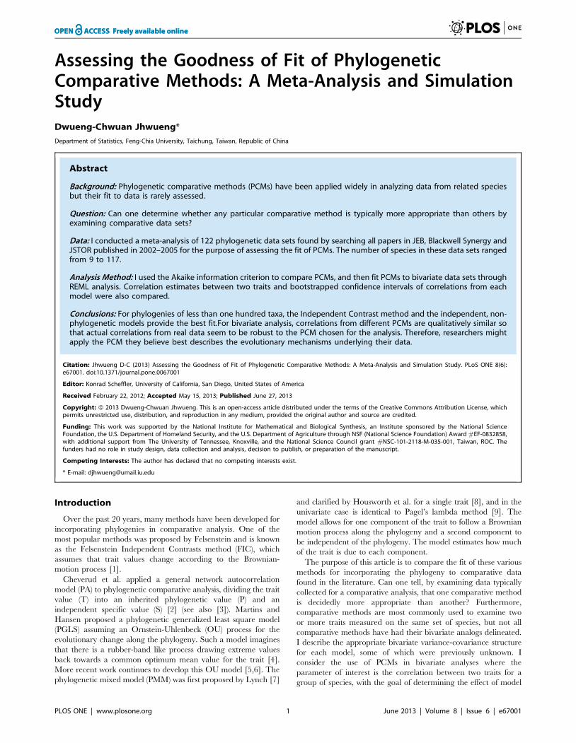
Assessing the Goodness of Fit of PhylogeneticComparative Methods: A Meta-Analysis and SimulationStudyDwueng-Chwuan Jhwueng*

Department of Statistics, Feng-Chia University, Taichung, Taiwan, Republic of China

Abstract

Background: Phylogenetic comparative methods (PCMs) have been applied widely in analyzing data from related speciesbut their fit to data is rarely assessed.

Question: Can one determine whether any particular comparative method is typically more appropriate than others byexamining comparative data sets?

Data: I conducted a meta-analysis of 122 phylogenetic data sets found by searching all papers in JEB, Blackwell Synergy andJSTOR published in 2002–2005 for the purpose of assessing the fit of PCMs. The number of species in these data sets rangedfrom 9 to 117.

Analysis Method: I used the Akaike information criterion to compare PCMs, and then fit PCMs to bivariate data sets throughREML analysis. Correlation estimates between two traits and bootstrapped confidence intervals of correlations from eachmodel were also compared.

Conclusions: For phylogenies of less than one hundred taxa, the Independent Contrast method and the independent, non-phylogenetic models provide the best fit.For bivariate analysis, correlations from different PCMs are qualitatively similar sothat actual correlations from real data seem to be robust to the PCM chosen for the analysis. Therefore, researchers mightapply the PCM they believe best describes the evolutionary mechanisms underlying their data.

Citation: Jhwueng D-C (2013) Assessing the Goodness of Fit of Phylogenetic Comparative Methods: A Meta-Analysis and Simulation Study. PLoS ONE 8(6):e67001. doi:10.1371/journal.pone.0067001

Editor: Konrad Scheffler, University of California, San Diego, United States of America

Received February 22, 2012; Accepted May 15, 2013; Published June 27, 2013

Copyright: � 2013 Dwueng-Chwuan Jhwueng. This is an open-access article distributed under the terms of the Creative Commons Attribution License, whichpermits unrestricted use, distribution, and reproduction in any medium, provided the original author and source are credited.

Funding: This work was supported by the National Institute for Mathematical and Biological Synthesis, an Institute sponsored by the National ScienceFoundation, the U.S. Department of Homeland Security, and the U.S. Department of Agriculture through NSF (National Science Foundation) Award #EF-0832858,with additional support from The University of Tennessee, Knoxville, and the National Science Council grant #NSC-101-2118-M-035-001, Taiwan, ROC. Thefunders had no role in study design, data collection and analysis, decision to publish, or preparation of the manuscript.

Competing Interests: The author has declared that no competing interests exist.

* E-mail: [email protected]

Introduction

Over the past 20 years, many methods have been developed for

incorporating phylogenies in comparative analysis. One of the

most popular methods was proposed by Felsenstein and is known

as the Felsenstein Independent Contrasts method (FIC), which

assumes that trait values change according to the Brownian-

motion process [1].

Cheverud et al. applied a general network autocorrelation

model (PA) to phylogenetic comparative analysis, dividing the trait

value (T) into an inherited phylogenetic value (P) and an

independent specific value (S) [2] (see also [3]). Martins and

Hansen proposed a phylogenetic generalized least square model

(PGLS) assuming an Ornstein-Uhlenbeck (OU) process for the

evolutionary change along the phylogeny. Such a model imagines

that there is a rubber-band like process drawing extreme values

back towards a common optimum mean value for the trait [4].

More recent work continues to develop this OU model [5,6]. The

phylogenetic mixed model (PMM) was first proposed by Lynch [7]

and clarified by Housworth et al. for a single trait [8], and in the

univariate case is identical to Pagel’s lambda method [9]. The

model allows for one component of the trait to follow a Brownian

motion process along the phylogeny and a second component to

be independent of the phylogeny. The model estimates how much

of the trait is due to each component.

The purpose of this article is to compare the fit of these various

methods for incorporating the phylogeny to comparative data

found in the literature. Can one tell, by examining data typically

collected for a comparative analysis, that one comparative method

is decidedly more appropriate than another? Furthermore,

comparative methods are most commonly used to examine two

or more traits measured on the same set of species, but not all

comparative methods have had their bivariate analogs delineated.

I describe the appropriate bivariate variance-covariance structure

for each model, some of which were previously unknown. I

consider the use of PCMs in bivariate analyses where the

parameter of interest is the correlation between two traits for a

group of species, with the goal of determining the effect of model

PLOS ONE | www.plosone.org 1 June 2013 | Volume 8 | Issue 6 | e67001

choice on the estimates of correlations. Are the correlation

estimates qualitatively concordant (having the same sign) or do the

methods give wildly different correlation estimates for given real

data sets?

Modifications are required to three of these methods in order

for the AIC comparisons to be valid [10]. I make a trivial

modification to FIC to get maximum likelihood rather than

restricted maximum likelihood estimates. I make a more

substantial modification to the autocorrelation model by not

normalizing the data in advance of determining its error structure.

As the OU process should recover the Brownian motion process

when the constraint parameter tends to zero, I make a

modification to the PGLS as given in [4] so that this property is

preserved. This same modification was used in [5].

Methods and Materials

Data SelectionI searched for published phylogenetic data sets in JEB, Blackwell

Synergy and JSTOR using the keywords: ((Comparative methods

OR Comparative analysis) AND independent contrasts) for 2002–

2005. I included only articles that contained a phylogeny and the

raw data for continuously distributed traits. All data sets contained

averaged trait values; some also provided sample sizes and

standard deviations or standard errors. These criteria yielded 43

articles, which were pruned further by eliminating studies where

the species were from more than one order (so as to increase the

chance that the species experienced a single model of evolution).

Note that the choice of order as the cut-off is arbitrary; other

authors have used other cutoffs such as families [11] and genera

[5]. The final assemblage of data sets included 122 traits (some

papers had multiple traits) and 47 phylogenetic trees. Data set size

ranged from 9 to 117 species. The flow of information through the

different phases of a systematic review is reported in Figure S1 in

supporting information section. The references for the data sets

are listed in Table [11–34].

The Phylogenetic Similarity Matrix GPCM approaches typically require a phylogeny with branch

lengths. To recover this, I used a ruler to measure the branch

lengths. Some of the phylogenies were chronograms, where

branch length is proportional to time, and others were cladograms;

the former would be expected to have better branch lengths for

PCM. I converted each phylogeny into a similarity matrix G. The

diagonal elements of G, gii,i~1,2, � � � ,n, represent the correlation

of a species with itself and so equal 1.0. The off-diagonal elements

gij ,i=j, represent the relative evolutionary time shared by two

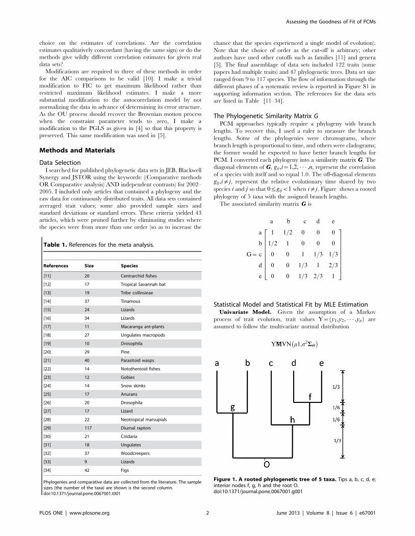
species i and j so that 0ƒgijv1 when i=j. Figure shows a rooted

phylogeny of 5 taxa with the assigned branch lengths.

The associated similarity matrix G is

a b c d e

G~

a

b

c

d

e

1 1=2 0 0 0

1=2 1 0 0 0

0 0 1 1=3 1=3

0 0 1=3 1 2=3

0 0 1=3 2=3 1

2666666664

3777777775

Statistical Model and Statistical Fit by MLE EstimationUnivariate Model. Given the assumption of a Markov

process of trait evolution, trait values Y~ y1,y2, � � � ,ynð Þ are

assumed to follow the multivariate normal distribution

Y ~MMVN m1,s2SH

� �

Figure 1. A rooted phylogenetic tree of 5 taxa. Tips a, b, c, d, e;interior nodes f, g, h and the root O.doi:10.1371/journal.pone.0067001.g001

Table 1. References for the meta analysis.

References Size Species

[11] 20 Centrarchid fishes

[12] 17 Tropical Savannah bat

[13] 19 Tribe collinsieae

[14] 37 Tinamous

[15] 24 Lizards

[16] 34 Lizards

[17] 11 Macaranga ant-plants

[18] 27 Ungulates macropods

[19] 10 Drosophila

[20] 29 Pine

[21] 40 Parasitoid wasps

[22] 14 Notothenioid fishes

[23] 12 Gobies

[24] 14 Snow skinks

[25] 17 Anurans

[26] 20 Drosophila

[27] 17 Lizard

[28] 22 Neotropical marsupials

[29] 117 Diurnal raptors

[30] 21 Cnidaria

[31] 18 Ungulates

[32] 37 Woodcreepers

[33] 9 Lizards

[34] 42 Figs

Phylogenies and comparative data are collected from the literature. The samplesizes (the number of the taxa) are shown is the second column.doi:10.1371/journal.pone.0067001.t001

Assessing the Goodness of Fit of PCMs


with the overall mean mand variance s2. 1~ 1,1, � � � ,1ð Þt is the

vector of ones.

Each PCM results in a different variance-covariance structure

Sh, for the data:

ID Sh~I , the identity matrix.

FIC Sh~G :

PMM Sh~Sh2~h2Gz 1{h2� �

I ,0ƒhƒ1.

PA Sh~Sr~ I{rWð Þ{1 I{rWð Þ{t,0ƒrƒ1.

OU Sh~Sa~e{2a 1{gijð Þ 1{e{2agij

2a,aw0,i,j~1,2, � � � ,n.

Several of the PCMs have a free parameter (h2 for PMM, r for

PA, a for OU); for simplicity, I refer to this parameter as h. Note

that for FIC, I make a trivial modification to get maximum

likelihood rather than restricted maximum likelihood estimates.

For PA, W is the connectivity matrix [2]. For OU, Sa is identical

to the covariance structure in [5].

The negative log likelihood function is

{ log L m,s2,hDY� �

~n

2log 2pz

n

2log s2z

1

2log DShDz

1

2s2Y{m1ð ÞtS{1

h Y{m1ð Þ

where jShj is the determinant of Sh.

The MLEs for the mean and variance are the function of

hwhere

mm~1tS{1

h Y

1tS{1h 1

,ss2~Y{mm1ð ÞtS{1

h Y{mm1ð Þn

, respectively.

The MLE estimator hh is obtained by optimizing the negative log

likelihood function { log L hjYð Þ on the domains: h[½0,1� for

PMM, r[½{1,1� for PA, and aw0 for OU, respectively.

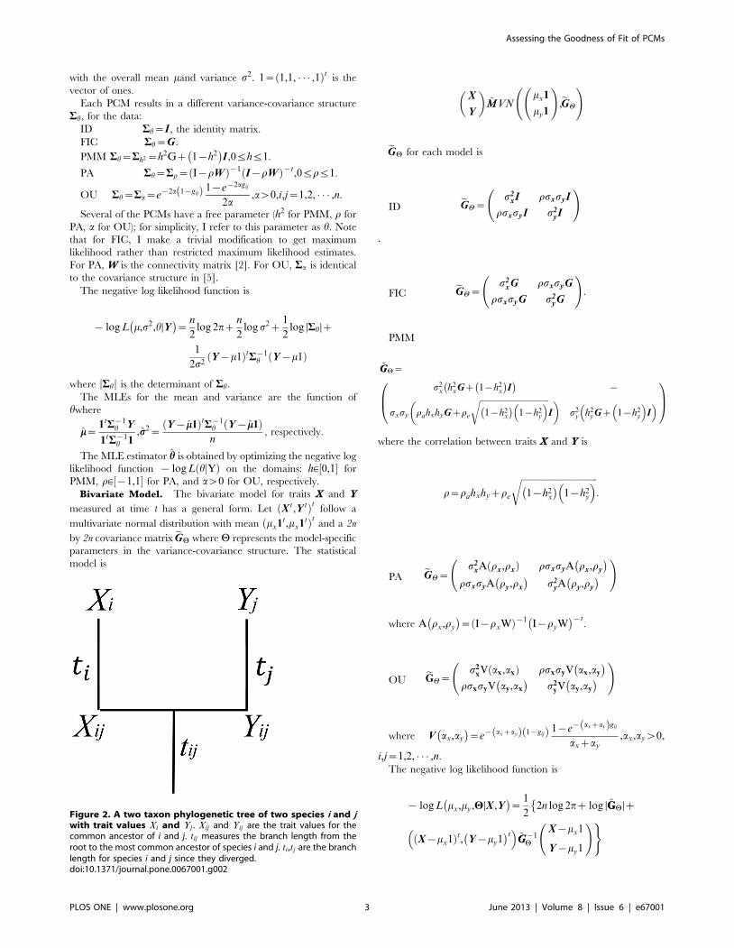
Bivariate Model. The bivariate model for traits X and Y

measured at time t has a general form. Let X t,Y tð Þt follow a

multivariate normal distribution with mean mx1t,mx1tð Þt and a 2n

by 2n covariance matrix eGH where H represents the model-specific

parameters in the variance-covariance structure. The statistical

model is

X

Y

� �~MMVN

mx1

my1

!,eGH

!

eGH for each model is

ID eGH~s2

xI rsxsyI

rsxsyI s2yI

!

.

FIC eGH~s2

xG rsxsyG

rsxsyG s2yG

!:

PMM

~GGH~

s2x h2

xGz 1{h2x

� �I

� �{

sxsy rahxhyGzre

ffiffiffiffiffiffiffiffiffiffiffiffiffiffiffiffiffiffiffiffiffiffiffiffiffiffiffiffiffiffiffiffiffiffi1{h2

x

� �1{h2

y

� �rI

� �s2

y h2yGz 1{h2

y

� �I

� �0B@

1CAwhere the correlation between traits X and Y is

r~rahxhyzre

ffiffiffiffiffiffiffiffiffiffiffiffiffiffiffiffiffiffiffiffiffiffiffiffiffiffiffiffiffiffiffiffiffiffi1{h2

x

� �1{h2

y

� �r:

PA eGH~s2

xA rx,rxð Þ rsxsyA rx,ry

� �rsxsyA ry,rx

� �s2

yA ry,ry

� � !

where A rx,ry

� �~ I{rxWð Þ{1

I{ryW� �{t

.

OU eGH~s2

xV ax,axð Þ rsxsyV ax,ay

� �rsxsyV ay,ax

� �s2

yV ay,ay

� � !

where V ax,ay

� �~e{ axzayð Þ 1{gijð Þ 1{e{ axzayð Þgij

axzay

,ax,ayw0,

i,j~1,2, � � � ,n.

The negative log likelihood function is

{ log L mx,my,HDX ,Y� �

~1

22n log 2pz log D~GGHDz

X{mx1ð Þt, Y{my1� �t

� �~GG{1H

X{mx1

Y{my1

!)Figure 2. A two taxon phylogenetic tree of two species i and jwith trait values Xi and Yj . Xij and Yij are the trait values for thecommon ancestor of i and j. tij measures the branch length from theroot to the most common ancestor of species i and j. ti ,tj are the branchlength for species i and j since they diverged.doi:10.1371/journal.pone.0067001.g002



where jeGHj is the determinant of eGH. I use restricted maximum

likelihood methods (REML) to estimate the correlation between

two traits, as adjusted by the effect of the phylogeny. REML

eliminates the need to estimate means and often produces less bias

in the variances and correlation estimators. I used Powell’s method

to optimize the maximum likelihood estimators (after reducing the

dimension of the search by solving for some parameters in terms of

others; details available upon request). This method uses one-

dimensional line searches in increasingly independent best

directions, while periodically resetting the directions to be

orthogonal. It is fast and efficient when the function is quadratic

or close to quadratic, as likelihood functions often are close to their

maximum [35–36]. There is no published maximum likelihood

method for bivariate PA and OU. To create one, I propose the

appropriate variance-covariance structure for these two methods:

PA:

The univariate phylogenetic autoregressive model proposed by

Cheverud et al. [2] adapted the spatial autocorrelation model in

[37]. The modified model I propose for univariate data analysis is

X{mx1~rxW X{mx1ð Þ

where ex~MMVN 0,s2

xI� �

and W is the phylogenetic connectivity

matrix with zeros on the diagonal and rows that sum to one. The

autocorrelation coefficient, rx, measures the impact of the

phylogenetic effect on the traits. The residual ex is independent

of rxW X{mx1ð Þ and can be regarded as the value gained or loss

due to non-phylogenetic component.

Transforming the equation, we have

X~mx1z I{rxWð Þ{1ex~MMVN mxr1,s2

x I{rxWð Þ{1I{rxWð Þ{t

� �

For bivariate analysis, let ex and ey be the residuals for the traits

X and Y, respectively. As in the univariate case, the residuals ex

and ey are independent of the phylogenetic components

rxW X{mx1ð Þ and ryW Y{my1� �

. I now assume the correlation

between the two residuals exists and let the correlation equal

tocov ex,ey

�~rI .

Then, the covariance between the pair of traits is

cov X ,Y½ �~cov mx1z I{rxWð Þ{1ex,my1z I{ryW� �{1

ey

h i~sxsy I{rxWð Þ{1

cov ex,ey

�I{ryW� �{t

~rsxsy I{rxWð Þ{1 I{ryW� �{t

:

The statistical model for the bivariate phylogenetic autoregres-

sive model is therefore,

X

Y

� �~MMVN

mx1

my1

!,

s2xA rx,rxð Þ rsxsyA rx,ry

� �rsxsyA ry,rx

� �s2

yA ry,ry

� � ! !

where A rx,ry

� �~ I{rxWð Þ{1 I{ryW

� �{t.

OU:

Martins and Hansen considered species evolving under the OU

process where a selection force pulls the trait back to an optimum.

Thus, the OU process can be used to model stabilizing selection

[4]. The univariate OU model assumes that the trait at time t, Xt,

satisfies

dXt~a m{Xtð ÞdtzsdBt

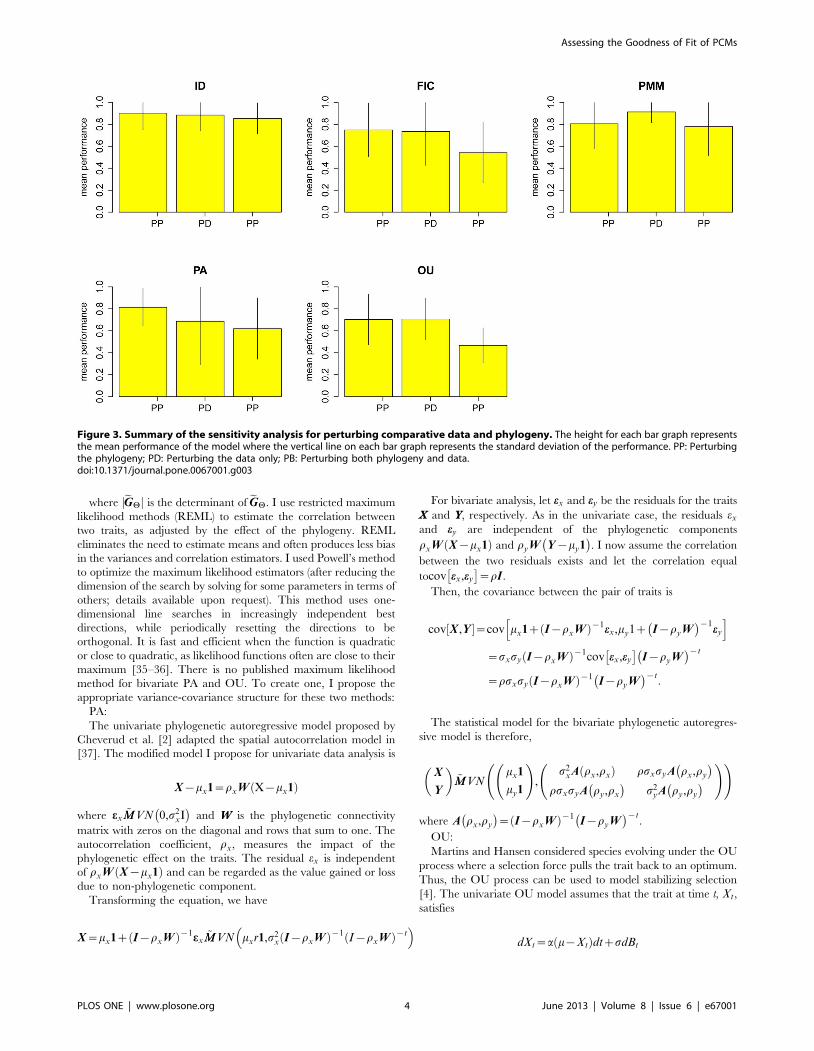
Figure 3. Summary of the sensitivity analysis for perturbing comparative data and phylogeny. The height for each bar graph representsthe mean performance of the model where the vertical line on each bar graph represents the standard deviation of the performance. PP: Perturbingthe phylogeny; PD: Perturbing the data only; PB: Perturbing both phylogeny and data.doi:10.1371/journal.pone.0067001.g003



Where a measures the magnitude selection force, m is the optimum

of the trait, and Bt is Brownian motion. The selection force acts

strongly towards the optimum when the trait is far from the

optimum and weakly if the trait is close to the optimum. For the

bivariate analog, there are two constraining force parameters, ax

for trait X and ay for trait Y.

Assuming that the constraining force parameters ax and ay are

constants during the evolutionary process, I propose the bivariate

statistical model

X

Y

� �~MMVN

mx1

my1

!,

s2xV ax,axð Þ rsxsyV ax,ay

� �rsxsyV ay,ax

� �s2

yV ay,ay

� � ! !

where V ax,ay

� �~e{ axzayð Þ 1{gij

� �1{e

{ axzayð Þgij

axzay

,ax,ayw0,

i,j~1,2, � � � ,n.

The covariance structure is developed by the following

mathematical property:

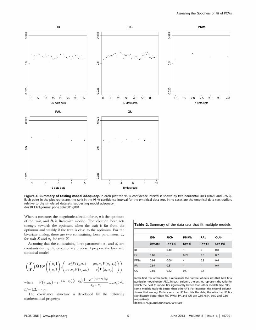
Figure 4. Summary of testing model adequacy. In each plot the 95 % confidence interval is shown by two horizontal lines (0.025 and 0.975).Each point in the plot represents the rank in the 95 % confidence interval for the empirical data sets. In no cases are the empirical data sets outliersrelative to the simulated datasets, suggesting model adequacy.doi:10.1371/journal.pone.0067001.g004

Table 2. Summary of the data sets that fit multiple models.

IDb FICb PMMb PAb OUb

(n = 36) (n = 67) (n = 4) (n = 5) (n = 10)

ID - 0.48 1 0 0.8

FIC 0.86 - 0.75 0.8 0.7

PMM 0.94 0.06 - 0.8 0.4

PA 0.89 0.81 1 - 0.9

OU 0.86 0.12 0.5 0.8 -

In the first row of the table, n represents the number of data sets that best fit aparticular model under AICc. In each column, the entries represent the ratio forwhich the best fit model fits significantly better than other models (see ‘‘Dosome models really fit better than others?’’). For instance, the second columnshows that among 36 data sets that ID best fits the data, the ratio that ID fitssignificantly better than FIC, PMM, PA and OU are 0.86, 0.94, 0.89 and 0.86,respectively.doi:10.1371/journal.pone.0067001.t002



Theorem 1. Let Xt and Yt,tw0 be two OU process random

variables. Given a rooted phylogeny for trait evolution, assuming

that the constraining force parameters ax and ay are constants

during the evolutionary process, the covariance between the trait

X of species i and the trait Y of species j is

cov Xi,Yj

�~rsxsye{axti e{aytj 1{e

{ axzayð Þtijaxzay

,i,j~1,2, � � � ,n

where tij measures the branch length from the root to the most

common ancestor of species i and j; ti, tj are the branch lengths for

species i and j since they diverged

(Figure 2). Proof of Theorem 1 is provided in appendix S1.

Model Selection for Univariate DataFor univariate data analysis, the fitted models were compared

using the Akaike Information Criteria (AIC), in order to measure

fit to data of a model [10].

AIC~2k{2 log L hhjY� �

where k is the number of parameters, L is the likelihood function,

and hh is the MLE estimator(s) in that model.

Hurvich and Tsai found AIC could over-fit models and be

biased if there are too many parameters in comparison to the

sample size. They proposed a modification of AIC when the ratio

of sample size to the number of parameter does not exceed 40

(n=kv40), AICc [38]:

AICc~AICz2k kz1ð Þn{k{1

Since n=k in this study is always less than 40, I used AICc for

model selection.

Another popular model selection method, Bayesian Information

criterion (BIC) where BIC~2 log n{2 log L hhjY� �

, is based on

an asymptotic result derived under the assumptions that the data

distribution is in the exponential family [39]. BIC is not

appropriate in model selection for biological phenotypic data sets

because, when sample size is small, BIC tends to select unfitted

models with large bias, which results in difficulty in inference [40].

SimulationDo Some Models really fit better than others? For a

given dataset, one can get a ranked list of models, including the

best model, by getting point estimates of AICc differences.

However, it is also useful to get the confidence intervals for these

differences. Thus, after determining which model fits a given data

set best, I proceeded to test whether it fits significantly better than

the other models by simulating the distribution of AICc

differences, using a procedure suggested in [40]. Given a set of

models indexed by i, define Di~AICci{AICcbest where

i~1,2, � � � ,M is the model index and the term best is the index

of the best model. In this study, i represents ID, FIC, PMM, PA, or

OU. I treated Di as a random variable and suggested the following

bootstrap technique for determining a confidence interval for Di. If

FIC is the best model for the data Y, generate new bootstrap

samples Y�b from FIC using the MLE from the original data. For

each sample, Y�b, determine the AICc values for each model. Let

min be the index of the model with smallest AICc value for the

bootstrapped data. Define the random variable D�b~AICcbest{AICcmin. I then order the Db in increasing order for

the B bootstrapping samples. Re-using the index b~1,2, � � � ,B but

for the ordered values, the 1{að Þ% confidence set for Di is CI =

½0,D 1{að ÞB�. If Di (the original difference for model i versus the best

model) falls outside this confidence interval, the null hypothesis

that the two models fit the data equally well is rejected and I

conclude that the best selected model under AICc is significantly

better than model i. I set B~1000 to get a reliable result on the

upper tail of D�b.

Robustness. The comparative data sets usually consist of

mean trait values derived from measuring a finite number of

samples, which are subject to both measurement and sampling

error. The phylogeny, even when given as a rooted molecular

clock tree, also has uncertainty in branch lengths and topology

because phylogenies are often obtained by a sample of DNA

sequences from the species involved. Accordingly, I consider the

robustness of my model selection results to perturbations of the

trait values and the phylogeny. Both procedures are described

below.

Perturbation of Comparative Data. Consider collecting m

samples from a particular species yielding trait values

y1,y2, � � � ,ym. Let se be the standard error and let �yy be the sample

mean. All of m, se, and �yy are typically reported in the studies used

in this analysis. I perturbed the species mean value by using the

formula �yy�~�yyzse:rtm{1�yy�where rt is a random sample from the t

distribution with m{1 degrees of freedom. This is a reasonable

approach because the sample mean will be approximately t-

distributed in most cases. However, biological data often follow a

log normal distribution with a natural bound of zero and with no

specific upper bound. On occasion, when the sample size is not

large and the underlying data are log normal, using

�yy�~�yyzse:rtm{1 to generate �yy�can give impossible (negative)

values with a substantial probability. Under such circumstances, I

apply an alternative resampling technique aimed at reproducing

the log normal data. Note that if y is a log normal random

variable, then x~ log y is a normal random variable. The second

order Taylor series approximation for the function x~ log y at the

point my is

x~ log y& log myz1

my

y{my

� �{

1

2m2y

y{my

� �2:

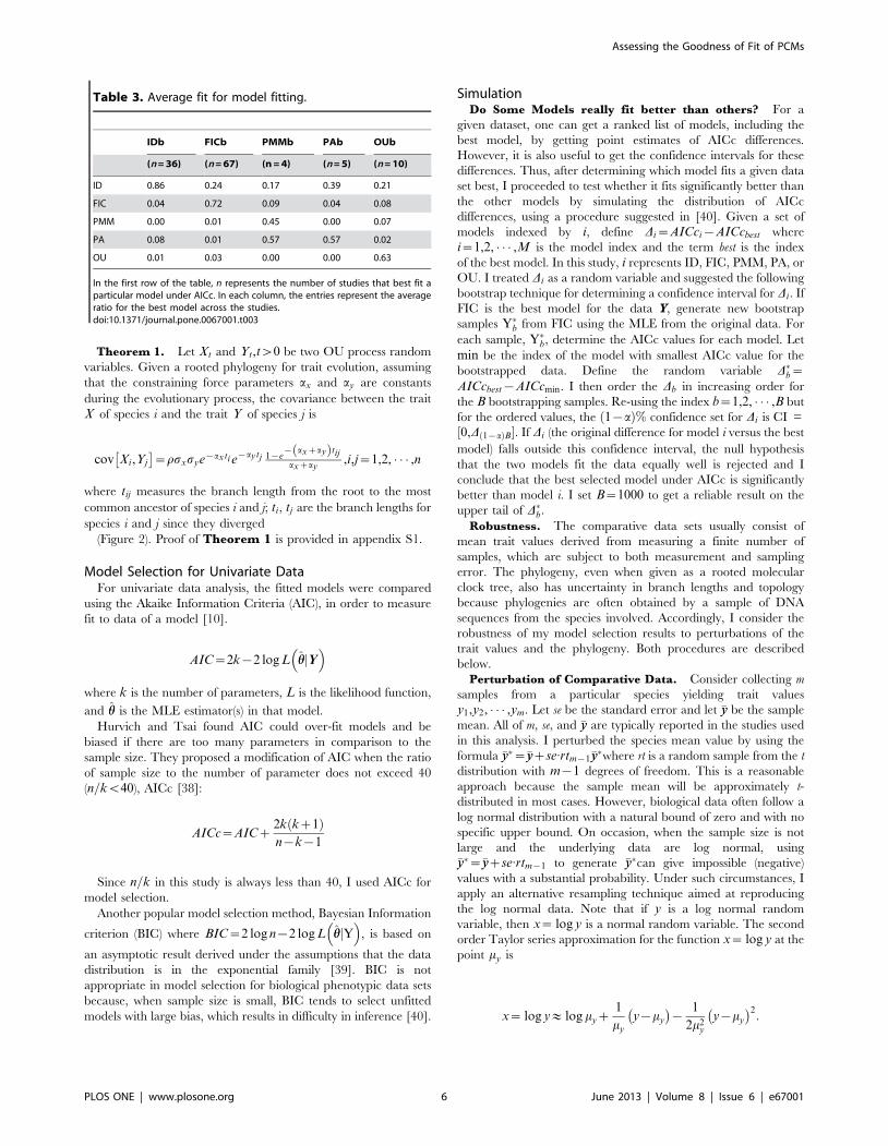
Table 3. Average fit for model fitting.

IDb FICb PMMb PAb OUb

(n = 36) (n = 67) (n = 4) (n = 5) (n = 10)

ID 0.86 0.24 0.17 0.39 0.21

FIC 0.04 0.72 0.09 0.04 0.08

PMM 0.00 0.01 0.45 0.00 0.07

PA 0.08 0.01 0.57 0.57 0.02

OU 0.01 0.03 0.00 0.00 0.63

In the first row of the table, n represents the number of studies that best fit aparticular model under AICc. In each column, the entries represent the averageratio for the best model across the studies.doi:10.1371/journal.pone.0067001.t003



Given the sample mean �yy and sample variance s2y for a log

normal variabley, the distribution of the normal variable x (with

mean mxand variance s2x) is approximately

mx~E log yð Þ& log my{1

2m2y

E y{my

� �2& log �yy{

1

2�yy2s2

y:

Using the linear part,

x~ log y& log myz1

my

y{my

� �;

the variance of x can be approximated as

s2x~var log yð Þ&

s2y

m2y

&s2

y

�yy2:

I sampled from the normal distribution with appropriate mean

and variance and exponentiated to get a sample from the log

normal distribution. For a sample of size m, I simulate

x�1,x�2, � � � ,x�m from normal distribution with mean log �yy{1

2�yy2

and variances2

y

�yy2. Then the perturbed data �yy� can be obtained as

�yy�~ 1m

Pmk~1

ex�

k :

Perturbation of Phylogeny. Stone considered the effect of

local phylogenetic perturbations on the regression fit. He studied

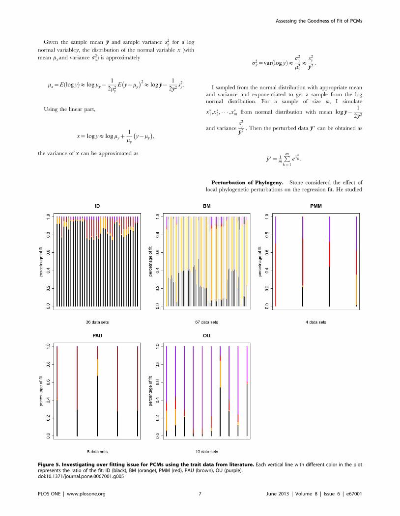
Figure 5. Investigating over fitting issue for PCMs using the trait data from literature. Each vertical line with different color in the plotrepresents the ratio of the fit: ID (black), BM (orange), PMM (red), PAU (brown), OU (purple).doi:10.1371/journal.pone.0067001.g005



how tree misspecification could influence the phylogenetic

regression given a Brownian motion model of evolution. He

found that branch length misspecification can be easily explained

in terms of the reweighting of contrast scores between subtrees

[41]. I used a likelihood-based approach rather than regression to

investigate how branch length misspecification could influence the

model selection. To do this, I first perturbed the phylogenetic tree

by randomly varying the branch lengths without changing the

topology. Recall that the phylogenetic tree is scaled so that the

length from the root to each tip is one. The unit length is

decomposed into d segments with lengths t1,t2, � � � ,tdð Þ by

identifying each ti as the time difference between two adjacent

nodes in the phylogenetic tree. Thus, ti,i~1,2, � � � ,d{1 are times

between the ithand the (iz1)th speciation events and td is the time

between the tip and the most recent node in the phylogenetic tree.

In terms of the entries of the relationship matrix G, let

1~gdwgd{1w � � �wg1~0 be the ranking of the distinct entries

in G, then we have ti~giz1{gi. To perturb the branch lengths

t1,t2, � � � ,tdð Þ but retain the topology of the original phylogeny,

the procedure is described in the following. I first treated

t1,t2, � � � ,tdð Þ as a d-dimensional random variable from a

Dirichlet distribution generated by drawing d independent

random samples, Ti,i~1,2, � � � ,d, each from a Gamma distribu-

tion with rate parameter kti,i~1,2, � � � ,d where k is an arbitrary

but positive constant. The desired d- tuple sample t�1,t�2, � � � ,t�d� �

from the Dirichlet distribution with parameter ktt1,ktt2, � � � ,kttdð Þis determined by

t�1,t�2, � � � ,t�d� �

~1Pd

i~1 Ti

T1,T2, � � � ,Tdð Þ:

Note that k is an arbitrary scaling variable that always preserves

the correct mean. That is,

E(t�i )~kti

kPd

i~1 ti

~kti

k~ti:

The Dirichlet distribution has a mode given by

Mt�i~

kti{1

k{d, where ktiw1,i~1,2, � � � ,d:

The choice of k is thus determined by min1ƒiƒd ktiw1.

I chose a positive integerk,

k~1

min1ƒiƒd ti

� where [a] returns the integer closest but less than a.

Because the mode Mt�i

of t�i is not equal to the expectation of t�i ,

such choice of k does not guarantee that the distribution of t�i is

centered or symmetric around its mean ti. The mode converges to

the expected mean when k approach to infinity (i.e.kti{1

k{d?ti as

k??). However, although choosing larger k helps to center the

distribution around ti, picking k too large will cause the samples t�ito be tightly centered around the given estimate tt. My choice of kis designed to be the minimal needed to prevent the phylogenetic

tree from varying too wildly from the given one while still

adequately testing robustness.

PCMs Comparison by Confidence Intervals for theCorrelation

For bivariate data analysis, I generated the confidence interval

by creating bivariate samples X�,Y� using the MLE estimators of

all the model parameters and re-estimating the correlation. I

created 1000 pairs of samples (X�i ,Y�i ),i~1,2, � � � ,1000 and

performed the REML analysis to obtain the

MLEsHHi,i~1,2, � � � ,1000. The 95 % confidence interval (CI) for

the correlation under the hypothesis testing is constructed from the

ordered MLEs for the correlation r�1vr�2v � � �vr�1000 with the

cut off CI = ½r�25,r�975�. The correlation is significantly positive at

the 5% level if r�25w0, significantly negative at the 5% level if

r�975v0 and otherwise not significantly different from zero at the

5% level.

Results

Model Selection under AICcI report the summary of the results from the simulation study in

Table 2. By the first row of Table 2, most of the data sets are best

described by either of the simplest models: the independent model

(ID) or by Brownian motion (FIC). The entire table shows the

performance of model-fitting of each model when competing with

other models. If the best fit model is independent (no phylogenetic

effect), then that model usually fits significantly better than other

models. However, if the model that best fits the data is Brownian

motion (FIC), then other models, except phylogenetic autocorre-

lation (PA), have a substantial probability of fitting the data as well.

For other parameter-rich models, PMM and OU usually fit

significantly better than other models; however, they do not fit

statistically significant better than each other. PA fits significantly

better than other models except for the independent (no

phylogenetic model).

Robustness for Models under Perturbing Data andPhylogeny

There were 64 traits for which standard error and sample size

were reported. For each trait, I simulate one thousand perturbed

data sets and phylogenies. The performance of the best model for

a trait is evaluated by proportion of simulated data sets on which

that model achieves the best fit. The mean performance is the

average value of the performances across studies. The results of the

perturbation analyses are shown in Figure 3. Data sets that best fit

by the independent model are the most robust to perturbations

while those whose best fit is a Brownian motion model (FIC) are

less robust. Data sets that are best fit by the Brownian motion

model (FIC), PMM, and OU seem to be more sensitive to

perturbations in the phylogeny than to perturbations in the

comparative data themselves.

Model Adequacy for PCMsI also evaluated model adequacy for PCMs. The purpose is to

investigate how well the model describes the underlying process

that generated the trait data. Essentially, if a model simulates

datasets that are indistinguishable from the observed datasets, the

model adequately describes the data. I first simulated a thousand

datasets by parametric bootstrapping using the MLE obtained

from the empirical data under each model and then re-evaluated

the likelihood from the simulated data for each model. The model

is considered inadequate if the log likelihood for the empirical data

falls out of the 95% confidence interval from the simulated data.

Figure 4 summarizes the result where scatter plots are shown to

examine the adequacy of the AIC best model. The likelihood for



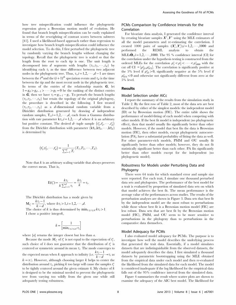
the empirical datasets falls well within the 95% confidence interval

for the simulated data from each model. Expressed as a percentile

of the simulated scores, the empirical data averaged in the 61st

percentile for ID, 62nd percentile for BM, 61st percentile for PMM,

66th percentile for PAU, and 63rd percentile for OU.

Figure 6. The confidence intervals of correlation for PCMs. Each line represents a confidence interval for a data set. Red lines include zerocorrelation in the confidence intervals.doi:10.1371/journal.pone.0067001.g006



Assessing Goodness of Fit for PCMsIt might be the model for fitting data is over fitted. To

investigate this, I simulate data using the true MLE under the best

model. Then the fit of other models is then evaluated.

The result is shown in Table 3 and Figure 5. The diagonal

entries in Table 3 show the average ratio of fit for the best model.

Datasets simulated under ID have ID as the best fitting model

86% of the time, FIC has the best fit 72% of time. For more

complicated models, datasets simulated under PMM have PMM

as the best fitting model 45% of the time, PA has the best fit 57 %

of time and OU has the best fit of 63 % of time which encounter

over fitting issue. For PMM, as the combination model of ID and

FIC, could be over fitted while the heritability parameter close to 0

or 1. In this case, ID and FIC would be the better fit. Similarly PA

is an extended model for ID where the zero autocorrelation is

detected.

Comparing Correlation Estimates from the PCMsI analyzed 225 bivariate data sets with 23 phylogenies. Figure 6

gives the comparison of the confidence intervals for correlations.

Correlations tend to be either positive or include zero in their

confidence intervals.

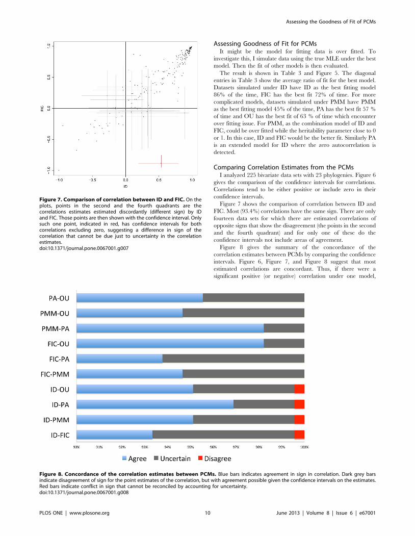
Figure 7 shows the comparison of correlation between ID and

FIC. Most (93.4%) correlations have the same sign. There are only

fourteen data sets for which there are estimated correlations of

opposite signs that show the disagreement (the points in the second

and the fourth quadrant) and for only one of these do the

confidence intervals not include areas of agreement.

Figure 8 gives the summary of the concordance of the

correlation estimates between PCMs by comparing the confidence

intervals. Figure 6, Figure 7, and Figure 8 suggest that most

estimated correlations are concordant. Thus, if there were a

significant positive (or negative) correlation under one model,

Figure 7. Comparison of correlation between ID and FIC. On theplots, points in the second and the fourth quadrants are thecorrelations estimates estimated discordantly (different sign) by IDand FIC. Those points are then shown with the confidence interval. Onlysuch one point, indicated in red, has confidence intervals for bothcorrelations excluding zero, suggesting a difference in sign of thecorrelation that cannot be due just to uncertainty in the correlationestimates.doi:10.1371/journal.pone.0067001.g007

Figure 8. Concordance of the correlation estimates between PCMs. Blue bars indicates agreement in sign in correlation. Dark grey barsindicate disagreement of sign for the point estimates of the correlation, but with agreement possible given the confidence intervals on the estimates.Red bars indicate conflict in sign that cannot be reconciled by accounting for uncertainty.doi:10.1371/journal.pone.0067001.g008



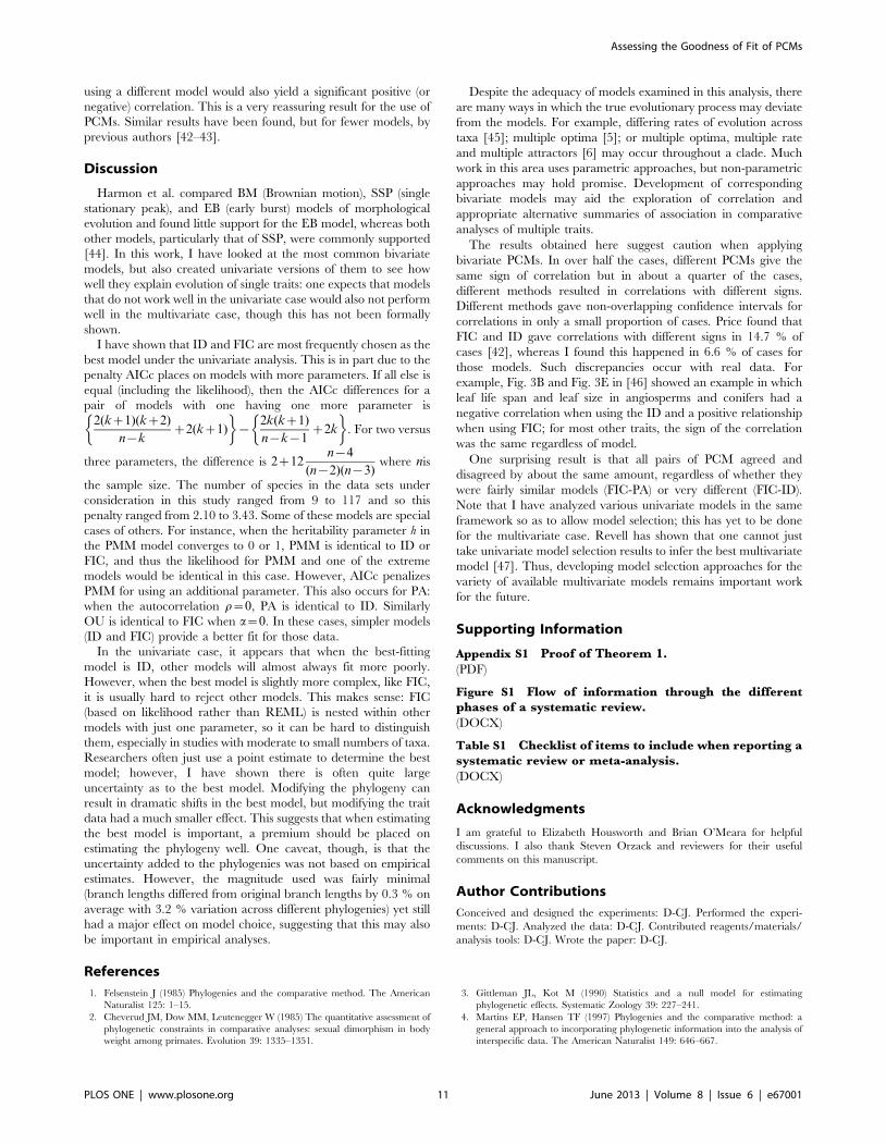
using a different model would also yield a significant positive (or

negative) correlation. This is a very reassuring result for the use of

PCMs. Similar results have been found, but for fewer models, by

previous authors [42–43].

Discussion

Harmon et al. compared BM (Brownian motion), SSP (single

stationary peak), and EB (early burst) models of morphological

evolution and found little support for the EB model, whereas both

other models, particularly that of SSP, were commonly supported

[44]. In this work, I have looked at the most common bivariate

models, but also created univariate versions of them to see how

well they explain evolution of single traits: one expects that models

that do not work well in the univariate case would also not perform

well in the multivariate case, though this has not been formally

shown.

I have shown that ID and FIC are most frequently chosen as the

best model under the univariate analysis. This is in part due to the

penalty AICc places on models with more parameters. If all else is

equal (including the likelihood), then the AICc differences for a

pair of models with one having one more parameter is

2(kz1)(kz2)

n{kz2(kz1)

� �{

2k(kz1)

n{k{1z2k

� �. For two versus

three parameters, the difference is 2z12n{4

(n{2)(n{3)where nis

the sample size. The number of species in the data sets under

consideration in this study ranged from 9 to 117 and so this

penalty ranged from 2.10 to 3.43. Some of these models are special

cases of others. For instance, when the heritability parameter h in

the PMM model converges to 0 or 1, PMM is identical to ID or

FIC, and thus the likelihood for PMM and one of the extreme

models would be identical in this case. However, AICc penalizes

PMM for using an additional parameter. This also occurs for PA:

when the autocorrelation r~0, PA is identical to ID. Similarly

OU is identical to FIC when a~0. In these cases, simpler models

(ID and FIC) provide a better fit for those data.

In the univariate case, it appears that when the best-fitting

model is ID, other models will almost always fit more poorly.

However, when the best model is slightly more complex, like FIC,

it is usually hard to reject other models. This makes sense: FIC

(based on likelihood rather than REML) is nested within other

models with just one parameter, so it can be hard to distinguish

them, especially in studies with moderate to small numbers of taxa.

Researchers often just use a point estimate to determine the best

model; however, I have shown there is often quite large

uncertainty as to the best model. Modifying the phylogeny can

result in dramatic shifts in the best model, but modifying the trait

data had a much smaller effect. This suggests that when estimating

the best model is important, a premium should be placed on

estimating the phylogeny well. One caveat, though, is that the

uncertainty added to the phylogenies was not based on empirical

estimates. However, the magnitude used was fairly minimal

(branch lengths differed from original branch lengths by 0.3 % on

average with 3.2 % variation across different phylogenies) yet still

had a major effect on model choice, suggesting that this may also

be important in empirical analyses.

Despite the adequacy of models examined in this analysis, there

are many ways in which the true evolutionary process may deviate

from the models. For example, differing rates of evolution across

taxa [45]; multiple optima [5]; or multiple optima, multiple rate

and multiple attractors [6] may occur throughout a clade. Much

work in this area uses parametric approaches, but non-parametric

approaches may hold promise. Development of corresponding

bivariate models may aid the exploration of correlation and

appropriate alternative summaries of association in comparative

analyses of multiple traits.

The results obtained here suggest caution when applying

bivariate PCMs. In over half the cases, different PCMs give the

same sign of correlation but in about a quarter of the cases,

different methods resulted in correlations with different signs.

Different methods gave non-overlapping confidence intervals for

correlations in only a small proportion of cases. Price found that

FIC and ID gave correlations with different signs in 14.7 % of

cases [42], whereas I found this happened in 6.6 % of cases for

those models. Such discrepancies occur with real data. For

example, Fig. 3B and Fig. 3E in [46] showed an example in which

leaf life span and leaf size in angiosperms and conifers had a

negative correlation when using the ID and a positive relationship

when using FIC; for most other traits, the sign of the correlation

was the same regardless of model.

One surprising result is that all pairs of PCM agreed and

disagreed by about the same amount, regardless of whether they

were fairly similar models (FIC-PA) or very different (FIC-ID).

Note that I have analyzed various univariate models in the same

framework so as to allow model selection; this has yet to be done

for the multivariate case. Revell has shown that one cannot just

take univariate model selection results to infer the best multivariate

model [47]. Thus, developing model selection approaches for the

variety of available multivariate models remains important work

for the future.

Supporting Information

Appendix S1 Proof of Theorem 1.

(PDF)

Figure S1 Flow of information through the differentphases of a systematic review.

(DOCX)

Table S1 Checklist of items to include when reporting asystematic review or meta-analysis.

(DOCX)

Acknowledgments

I am grateful to Elizabeth Housworth and Brian O’Meara for helpful

discussions. I also thank Steven Orzack and reviewers for their useful

comments on this manuscript.

Author Contributions

Conceived and designed the experiments: D-CJ. Performed the experi-

ments: D-CJ. Analyzed the data: D-CJ. Contributed reagents/materials/

analysis tools: D-CJ. Wrote the paper: D-CJ.

References

1. Felsenstein J (1985) Phylogenies and the comparative method. The American

Naturalist 125: 1–15.

2. Cheverud JM, Dow MM, Leutenegger W (1985) The quantitative assessment of

phylogenetic constraints in comparative analyses: sexual dimorphism in body

weight among primates. Evolution 39: 1335–1351.

3. Gittleman JL, Kot M (1990) Statistics and a null model for estimating

phylogenetic effects. Systematic Zoology 39: 227–241.

4. Martins EP, Hansen TF (1997) Phylogenies and the comparative method: a

general approach to incorporating phylogenetic information into the analysis of

interspecific data. The American Naturalist 149: 646–667.



5. Butler MA, King AA (2004) Phylogenetic comparative analysis: a modeling

approach for adaptive evolution. American Naturalist 164: 683–695.6. Beaulieu JM, Jhwueng DC, Boettiger C, O’Meara BC (2012) Modeling

stabilizing selection: expanding the Ornstein-Uhlenbeck model of adaptive

evolution. Evolution 66: 2369–2383.7. Lynch M (1991) Methods for the analyses of comparative data in evolutionary

biology. Evolution 45: 1065–1080.8. Housworth EA, Martins EP, Lynch M (2004) The phylogenetic mixed model.

The American Naturalist 163: 84–96.

9. Freckleton RP, Harvey PH, Pagel M (2002) Phylogenetic analysis andcomparative data. The American Naturalist 160: 712–726.

10. Akaike H (1974) A new look at the statistical identification model. IEEETransactions on Automatic Control 19: 716–723.

11. Collar DC, Near TJ, Wainwright PC (2005) Comparative analysis ofmorphological diversity: does disparity accumulate at the same rate in two

lineages of centrarchid fishes? Evolution 59: 1783–1794.

12. Aguirre L, Herrel A, Damme RV, Matthysen E (2002) Ecomorphologicalanalysis of trophic niche partitioning in a tropical savannah bat community.

Proceedings of the Royal Society B 269: 1271–1278.13. Armbruster WS, Mulder CPH, Baldwin BG, Kalisz S, Wessa B, et al. (2002)

Comparative analysis of late floral development and mating-system evolution in

tribe Collinsieae (Scrophulariaceae s.l.). American Journal of Botany 89: 37–49.14. Bertelli S, Tubaro PL (2002) Body mass and habitat correlates of song structure

in a primitive group of birds. Biological Journal of the Linnean Society 77: 423–430.

15. Bonnie KE, Gleeson TT, Garland T Jr (2005) Muscle fiber-type variation inlizards (Squamata) and phylogenetic reconstruction of hypothesized ancestral

states. The Journal of Experimental Biology 208: 4529–4547.

16. Cruz FB, Fitzgrald LA, Esponoza RE, Schulte JA (2005) The importance ofphylogenetic scale in tests of Bergmann’s and Rapoport’s rules: lessons from a

clade of South American lizards. Journal of Evolutionary Biology 18: 1559–1574.

17. Federle W, Rheindt FE (2005) Macaranga ant-plants hide food from intruders:

correlation of food pre-sentation and presence of wax barriers analysed usingphylogenetically independent contrasts. Biological Journal of the Linnean

Society 84: 177–193.18. Fisher DO, Blomberg SP, Owens IPF (2002) Convergent maternal care

strategies in ungulates and macropods. Evolution 56: 167–176.19. Gibbs AG, Fukuzato F, Matzkin LM (2003) Evolution of water conservation

mechanisms in Drosophila. The Journal of Experimental Biology 206: 1183–

1192.20. Grotkopp E, Rejmanek M, Rost TL (2002) Toward a causal explanation of plant

invasiveness: seedling growth and life-history strategies of 29 pine (Pinus) species.The American Naturalist 159: 396–419.

21. Jervis MA, Ferns PN, Heimpel GE (2003) Body size and the timing of egg

production in parasitoid wasps: a comparative analysis. Functional Ecology 17:375–383.

22. Johnston IA, Fernadez DA, Calvo J, Vieira VLA, North AW, et al. (2003)Reduction in muscle fibre number during the adaptive radiation of notothenioid

fishes: a phylogenetic perspective. The Journal of Experimental Biology 206:2595–2609.

23. Mazzoldi C, Petersen CW, Rasotto MB (2005) The influence of mating system

on seminal vesicle variability among gobies (Teleostei, Gobiidae). Journal ofZoological Systematics and Evolutionary Research 43: 307–314.

24. Melville J, Swain R (2003) Evolutionary correlations between escape behaviourand performance ability in eight species of snow skinks (Niveoscincus: Lygosominae)

from Tasmania. Journal of Zoology, London. 261: 79–89.

25. Monnet J M, Cherry MI (2002) Sexual size dimorphism in anurans. Proceedings

of the Royal Society B 269: 2301–2307.26. Moreteau1 B, Gibert P, Petavy G, Moreteau, GC, Huey RB, et al. (2003)

Morphometrical evolution in a Drosophila clade: the Drosophila obscura group.

Journal of Zoological Systematics and Evolutionary Research 41: 64–71.27. Niewiarowski PH, Angilletta MJ Jr, Leache AD (2004) Phylogenetic comparative

analysis of life-history variation among populations of the lizard Sceloporus

undulates: an example and prognosis. Evolution 58: 619–633.

28. Olifiers N, Vieira MV, Grelle CEV (2004) Geographic range and body size in

neotropical marsupials. Global Ecology and Biogeography 13: 439–444.29. Roulin A, Wink M (2004) Predator-prey relationships and the evolution of

colour polymorphism: a comparative analysis in diurnal raptors. BiologicalJournal of the Linnean Society 81: 565–578.

30. Sanchez JA, Lasker HR (2003) Patterns of morphological integration in marinemodular organisms: supra-module organization in branching octocoral colonies.

Proceedings of the Royal Society B 270: 2039–2044.

31. Toıgo C, Maillard JM (2003) Causes of sex-biased adult survival in ungulates:sexual size dimorphism, mating tactic or environment harshness? Oikos 101:

376–384.32. Tubaro PL, Lijtmaer DA, Palacios MG, Kopuchian C (2002) Adaptive

modification of tail structure in relation to body mass and buckling in

woodcreepers. The Condor 104: 281–296.33. Vanhooydonck B, Damme RV, Aert P (2002) Variation in speed, gait

characteristics and microhabitat use in lacertid lizards. The Journal ofExperimental Biology 205: 1037–1046.

34. Weiblen GD (2004) Correlated evolution in fig pollination. Systematic Biology53: 128–139.

35. Powell MJD (1964) An efficient method for finding the minimum of a function of

several variables without calculating derivatives, Computer Journal, 7: 155–162.36. Press WH, Teukolsky SA, Vetterling WT, Flannery BP (2007) ‘‘Section 10.7.

Direction Set (Powell’s) Methods in Multidimensions’’. Numerical Recipes: TheArt of Scientific Computing (3rd ed.). New York: Cambridge University Press.

ISBN 978-0-521-88068-8.

37. Ord JK (1975) Estimation Methods for Models of Spatial Interaction, Journal ofthe American Statistical Association 70: 120–126.

38. Hurvich CM, Tsai C-L (1989) Regression and time series model selection insmall samples. Biometrika 76: 297–307.

39. Schwarz G (1978) Estimating the dimension of a model. The Annals of Statistics6: 461–464.

40. Burham KP, Anderson DR (2002) Model selection and multimodel inference.

Springer-Verlag New York.41. Stone EA (2011) Why the phylogenetic regression appears robust to tree

misspecification Systematic Biology 2011, 60: 245–260.42. Price T (1997) Correlated evolution and independent contrasts. Philosophical

Transactions of the Royal Society B: Biological Sciences. 352: 519–529.

43. Martins EP, Hansen TF (1996) Phylogenies, spatial autoregression, and thecomparative method: a computer simulation test. Evolution 50: 1750–1765.

44. Harmon LJ, Losos JB, Davies TJ, Gillespie RG, Gittleman JL, et al. (2010) Earlybursts of body size and shape evolution are rare in comparative data. Evolution

64: 2385–2396.45. O’Meara BC, Ane C, Sanderson MJ, Wainwright PC (2006) Testing for

different rates of continuous trait evolution. Evolution 60: 922–933.

46. Ackerly DD, Reich P (1999) Convergence and correlations among leaf size andfunction in seed plants: a comparative test using independent contrasts.

American Journal of Botany 86: 1272–1281.47. Revell LJ (2010) Phylogenetic signal and linear regression on species data.

Methods in Ecology and Evolution 1: 319–329.



Assessing the Goodness of Fit of Phylogenetic Comparative Methods: A Meta-Analysis and Simulation...

Documents

Transcript of Assessing the Goodness of Fit of Phylogenetic Comparative Methods: A Meta-Analysis and Simulation...