GOODNESS OF FIT USING SPSS

WHAT IS GOODNESS OF FIT ?A goodness-of-fit is a statistical technique . It is

Applied to measure “how well the actual(observed) data pointsFit into a Machine Learning model ” . It summarizes the divergence between actual observed data points and expected data points in context to a statistical or machine learning model.

Assessment of divergence between the observed data points and model predicted data points is critical to understand , a decision made o poorly fitting models might be badly misleading. A seasoned practitioner must examine the fitment of actual and model predicted data points.

2

WHY DO WE TEST GOODNESS OF FIT ?Goodness-of-fit tests are statistical tests to

determine values match those predicted by the model . Goodness-of-fit tests are frequently applied in business decision making .

WHAT ARE THE MOST COMMMON GOODNESS OF FIT TEST ?FIT TEST ?

There are multiple methods for determining goodness-of-fit. Some of the most popular methods used in statistics include the chi-square, the Kolmogorov - Smirnov test, the Anderson-Darling test and the Shipiro - Wilk test.

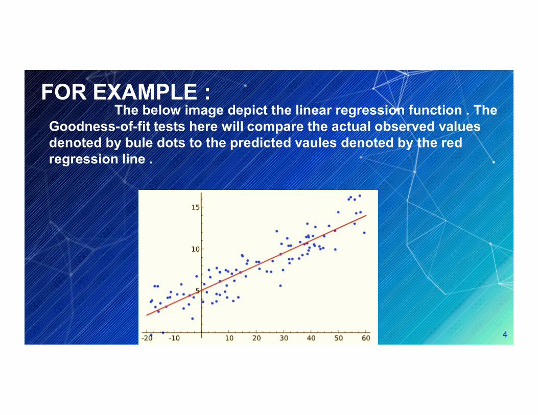
FOR EXAMPLE :The below image depict the linear regression function . The Goodness-of-fit tests here will compare the actual observed values denoted by bule dots to the predicted vaules denoted by the red regression line .

4

EXPLAIN TWO TEST ONLY1 . CHI – SQUARE TEST GOODNESS OF FIT USING SPSS

5

SPSS2 . NORMAL DISTRIBUTION FIT USING SPSS

1. CHI – SQUARE TEST FOR GOODNESS OF FIT USING SPSS

Chi-Square goodness of fit test is a non-parametric test that is used to find out how the observed value of a given phenomena is significantly different from the expected value. In Chi-Square goodness of fit test, the term goodness of fit is used to compare the observed sample distribution with the expected probability distribution. Chi-Square distribution with the expected probability distribution. Chi-Square goodness of fit test determines how well theoretical distribution (such as normal, binomial, or Poisson) fits the empirical distribution. In Chi-Square goodness of fit test, sample data is divided into intervals. Then the numbers of points that fall into the interval are compared, with the expected numbers of points in each interval.

6

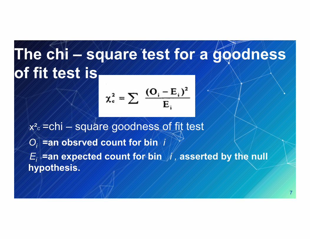
The chi – square test for a goodness of fit test is

x²C =chi – square goodness of fit test Oi =an obsrved count for bin iEi =an expected count for bin i , asserted by the null hypothesis.

7

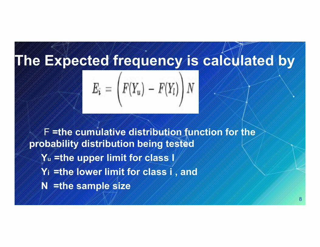
The Expected frequency is calculated by

F =the cumulative distribution function for the probability distribution being tested

Yu =the upper limit for class IYi =the lower limit for class i , and N =the sample size

8

Application of Chi-square as thegoodness of fit

The Chi-square is applied to establish or refute that a relationship exists between actual observed values and predicted values. The chi-squared test is a very useful tool predicted values. The chi-squared test is a very useful tool for predictive analytics professionals. It is used very commonly in Clinical research, Social sciences, and Business research .

It is also right tail test.9

Procedure for Chi-Square Goodness of Fit Test:HYPOTHESIS :Null Hypothesis : H0 There is no diference between observed and expected hypothesisAlternative Hypothesis : H1 There is a significant difference between observed and expected hypothesis

Example of chi – square goodness of fit test in SPSSA shop owner claims that an epual numbers of customers come into his shop each weekday. To test his Hypothesis , a researcher records the number of customers that come into the shop on a given week and Find the following.

Monday-50 customersMonday-50 customersTuesday-60 customersWednesday-40 customersThursday-47 customersFriday-53 customers

Use the following steps to perform a Chi-Square goodness of fit test in SPSS to Determine if the data is consistent with the shop owner’s claims.

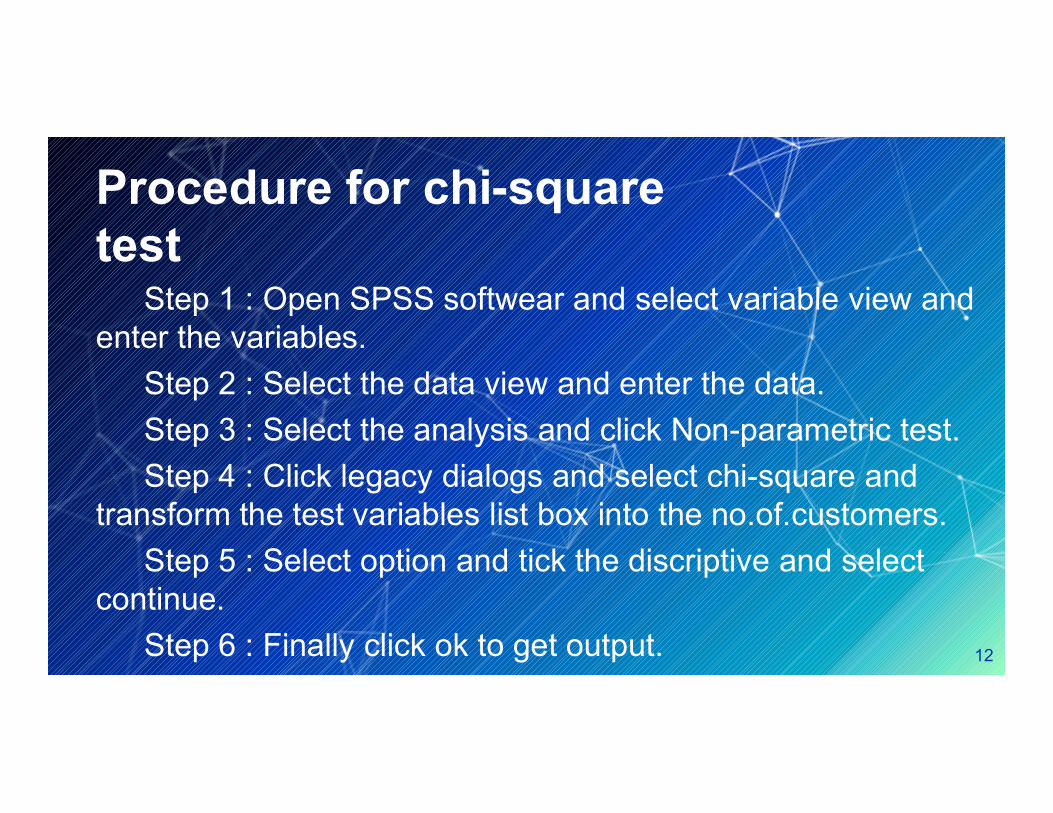
Procedure for chi-square test

Step 1 : Open SPSS softwear and select variable view and enter the variables.

Step 2 : Select the data view and enter the data. Step 3 : Select the analysis and click Non-parametric test.Step 4 : Click legacy dialogs and select chi-square and

transform the test variables list box into the no.of.customers.Step 5 : Select option and tick the discriptive and select

continue.Step 6 : Finally click ok to get output. 12

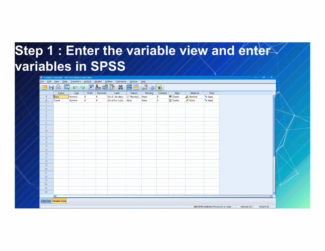
Step 1 : Enter the variable view and enter variables in SPSS

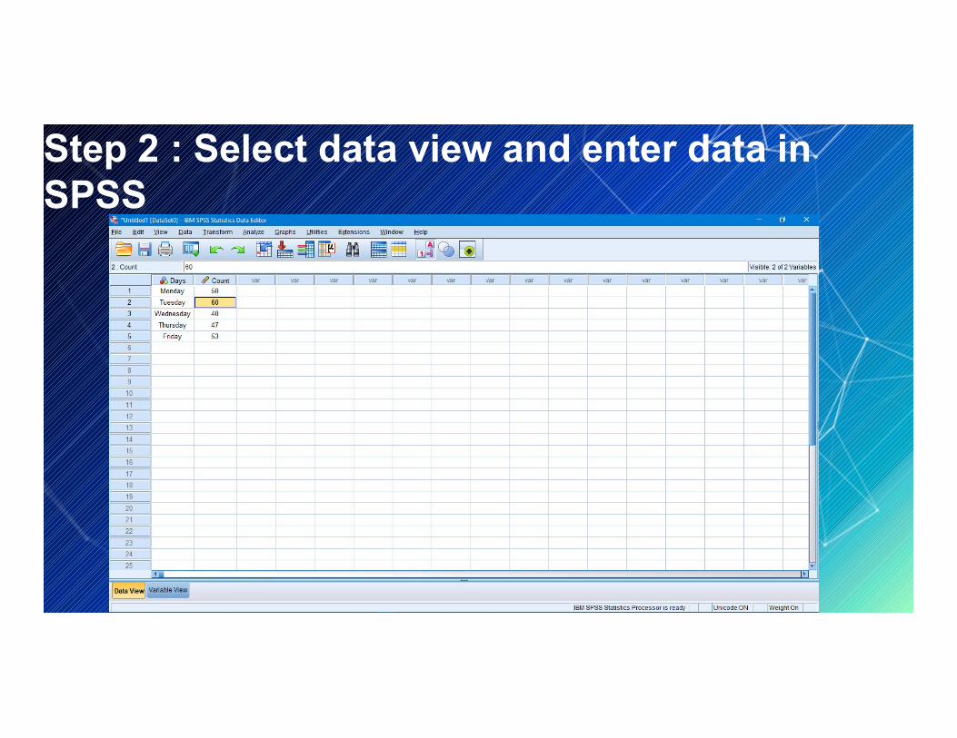
Step 2 : Select data view and enter data in SPSS

Step 3 : Select the analysis and click Non-parametric test and Click legacy dialogs and select chi-square.

Step 4 : transform the test variables list box into the no . Of . customers

Step 5 : Select option and tick the discriptiveand select continue and click ok.

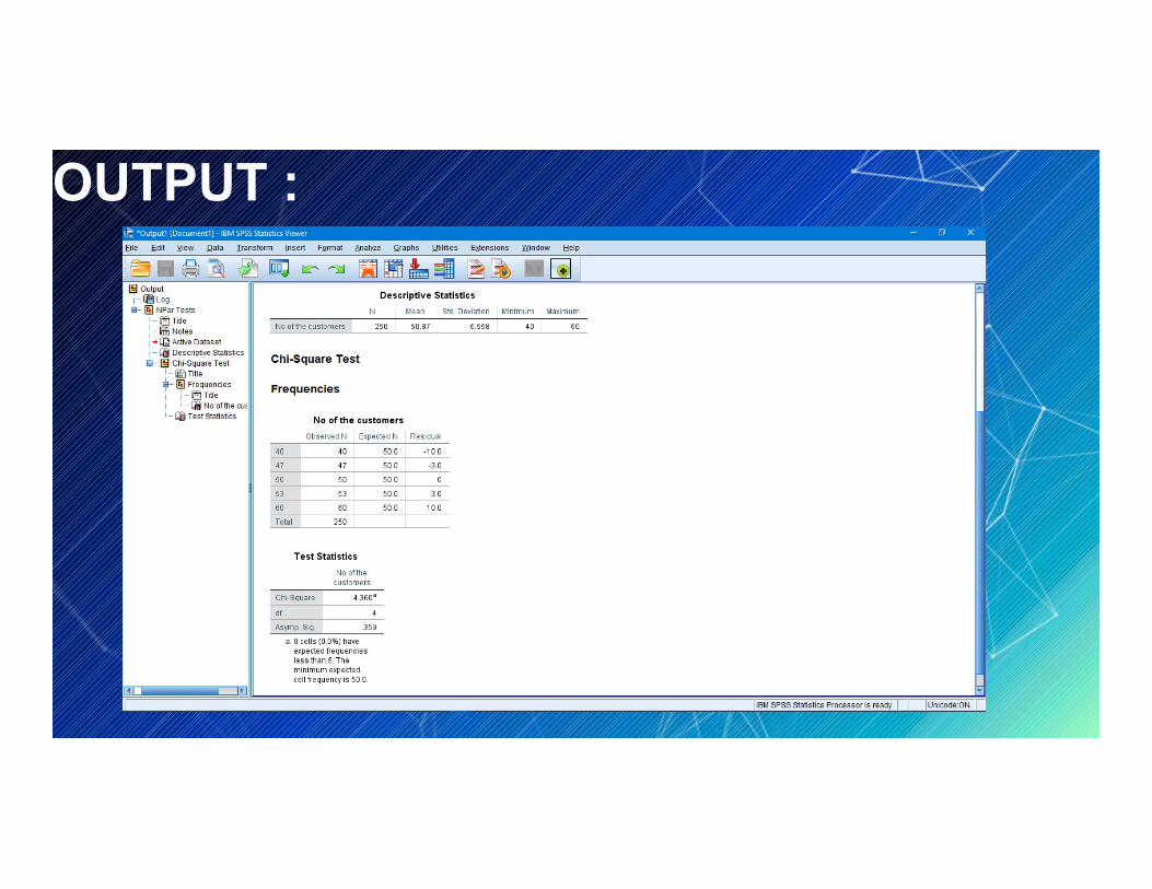
OUTPUT :

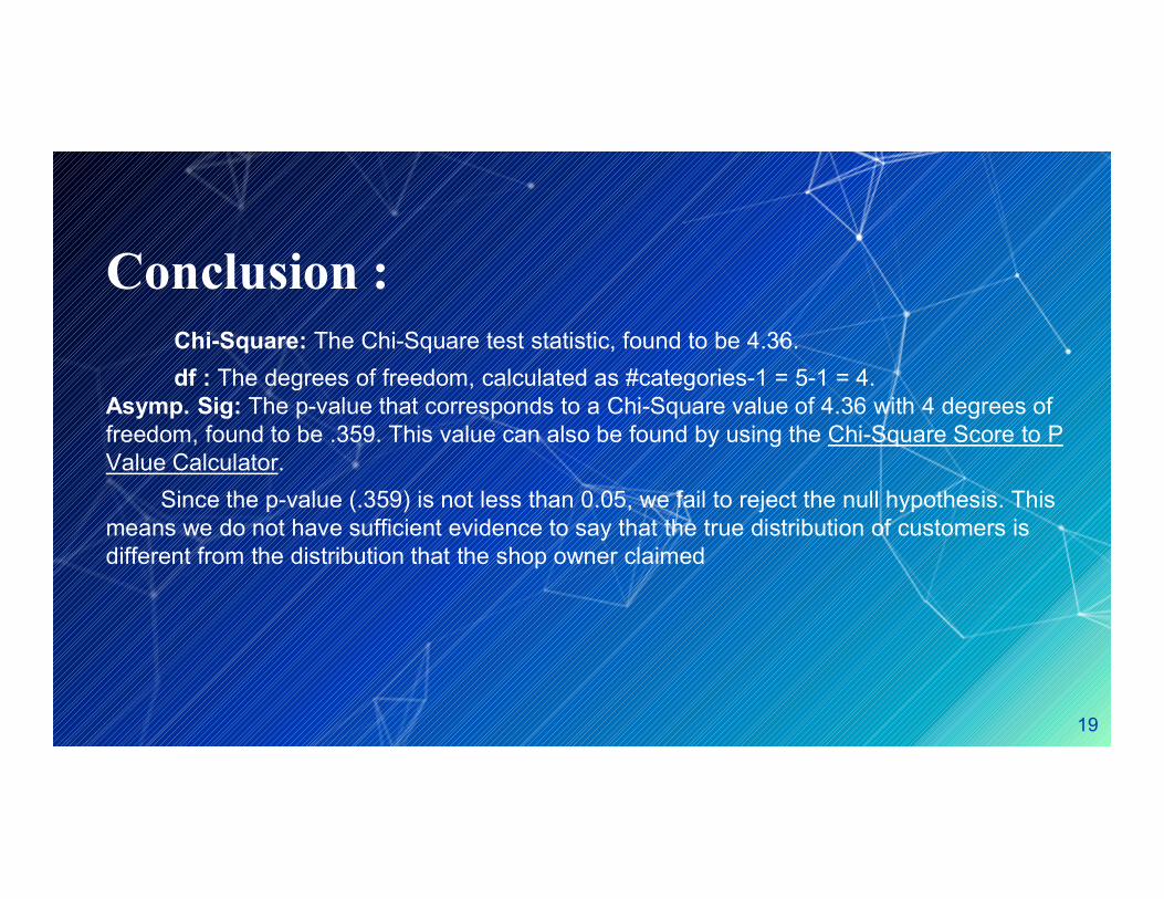
Conclusion :Chi-Square: The Chi-Square test statistic, found to be 4.36.df : The degrees of freedom, calculated as #categories-1 = 5-1 = 4.

Asymp. Sig: The p-value that corresponds to a Chi-Square value of 4.36 with 4 degrees of freedom, found to be .359. This value can also be found by using the Chi-Square Score to P Value Calculator.

Since the p-value (.359) is not less than 0.05, we fail to reject the null hypothesis. This means we do not have sufficient evidence to say that the true distribution of customers is different from the distribution that the shop owner claimed

19

2 . NORMAL DISTRIBUTION FIT USING IN SPSSNormality test using SPSS :

An normality test is used to determine whether sample data has been drawn from a normal distribute population.

What is Normal distribution ?The normal distribution is always symmetrical about the

mean which look like a “bell curve”.When testing for normality:• Probabilities > 0.05 indicate that the data are normal.• Probabilities < 0.05 indicate that the data are NOT normal.

20

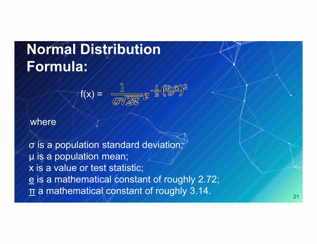
Normal Distribution Formula:

f(x) =

wherewhereσ is a population standard deviation;μ is a population mean;x is a value or test statistic;e is a mathematical constant of roughly 2.72;π a mathematical constant of roughly 3.14. 21

The following numerical and visual output must be investigated :

- Skewness and kurtosis z-values(should be somewhere in the span of -1.96 to +1.96)

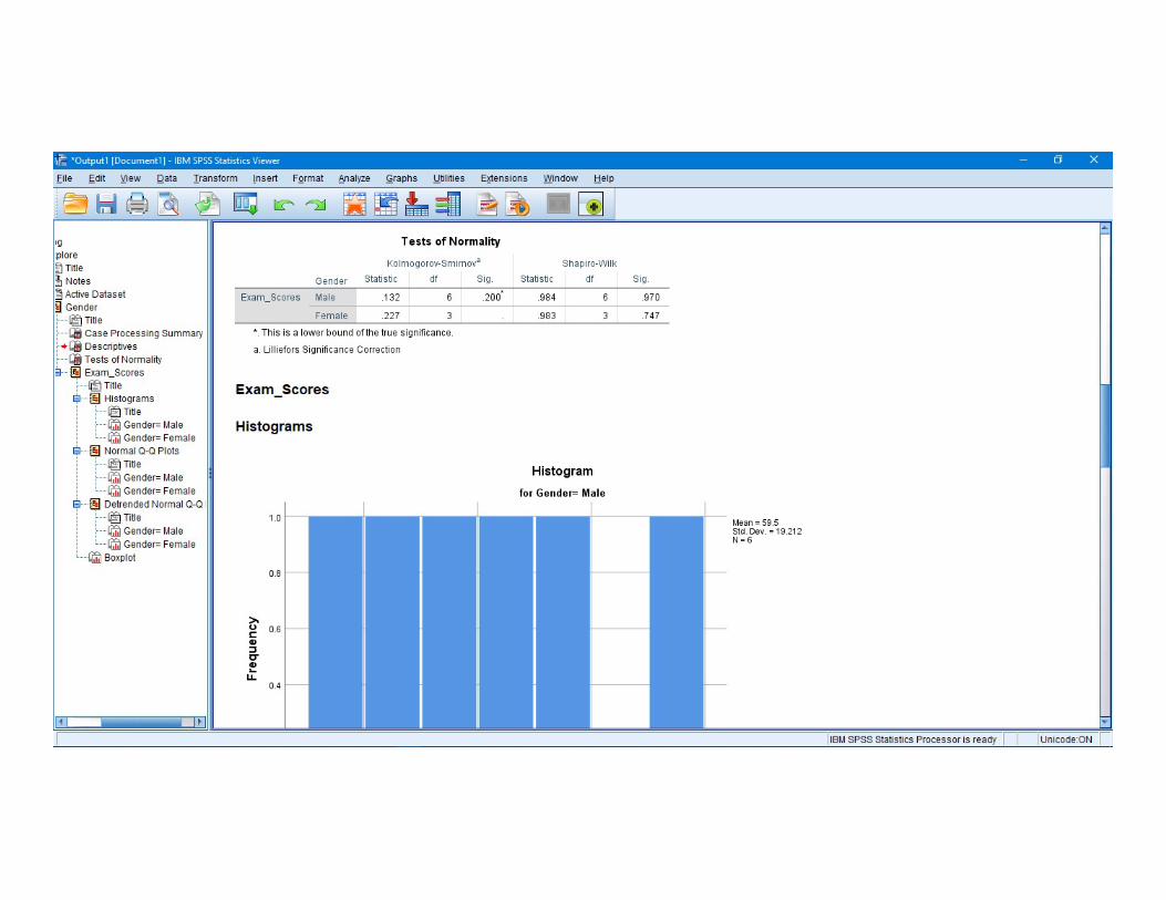
- The shapiro-wilk test p-value(should be above 0.05)

- Histograms , normal Q-Q plots and Box plots- Histograms , normal Q-Q plots and Box plots(should be indicated that our data are approximately normal

Distributed).

22

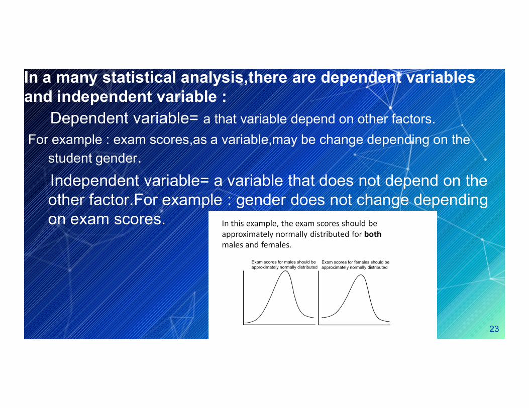
In a many statistical analysis,there are dependent variables and independent variable :

Dependent variable= a that variable depend on other factors.For example : exam scores,as a variable,may be change depending on the

student gender.Independent variable= a variable that does not depend on the other factor.For example : gender does not change depending other factor.For example : gender does not change depending on exam scores.

23

Example:The studentsGender = male and femaleExam scores = 47,53,60,90,70,45,35,62,84,Exam scores = 47,53,60,90,70,45,35,62,84,

24

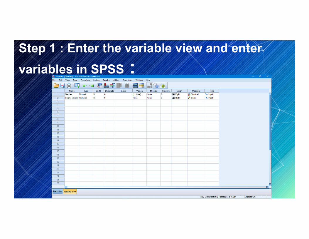
Step 1 : Enter the variable view and enter variables in SPSS :

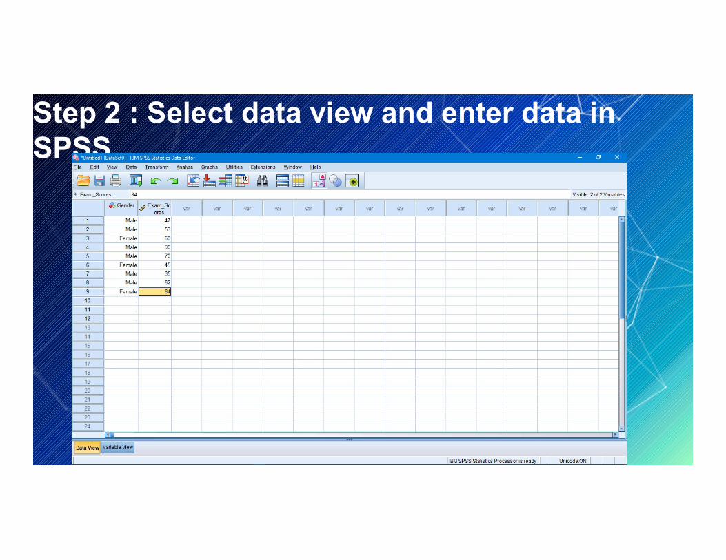
Step 2 : Select data view and enter data in SPSS

Step 3 : Select the analysis and click discriptivestatistics and select explore :

Step 4 : transform the Dependent list box into the Exam_scores and transform the Factor list box into the Gender

Step 5 : Open polts and ticks histogram and normality plots with test and continue then click ok .

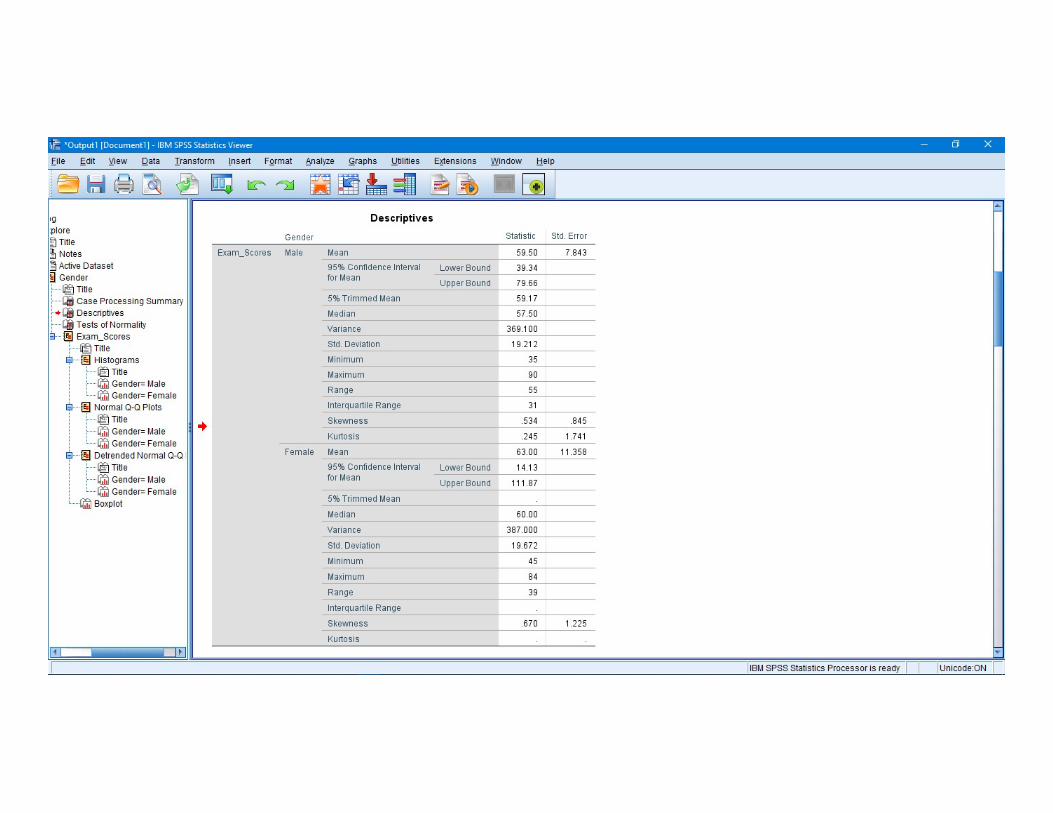
OUTPUT :

31

32

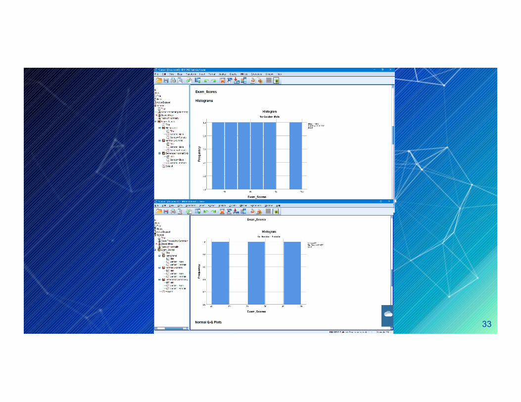
33

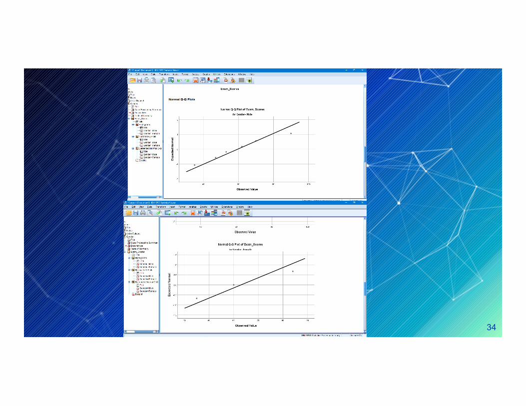
34

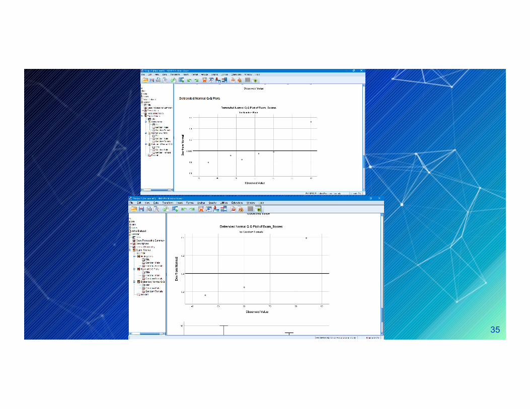
35

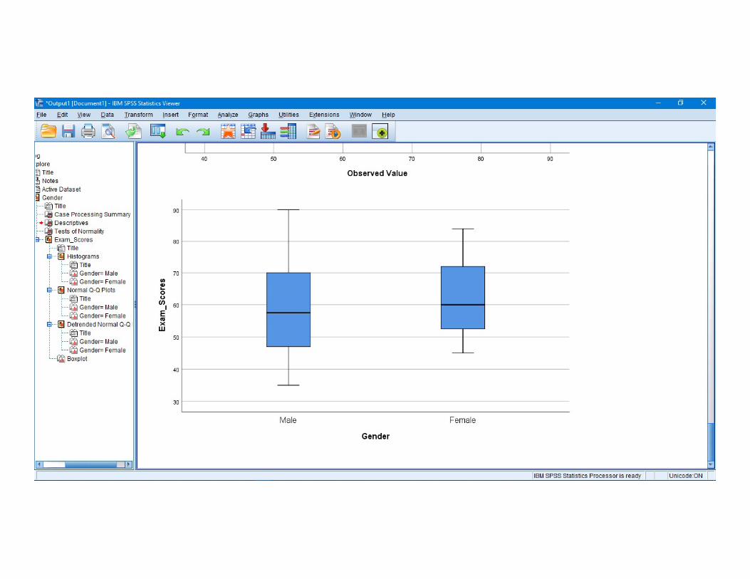
36

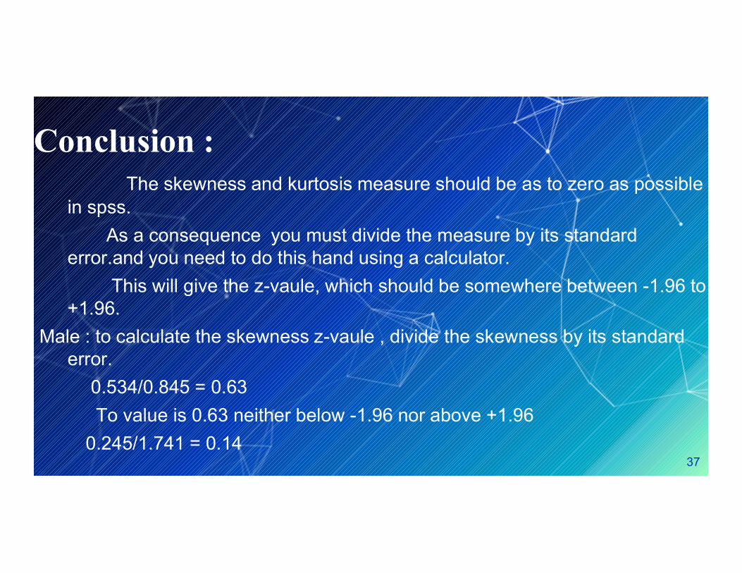
Conclusion :The skewness and kurtosis measure should be as to zero as possible

in spss.As a consequence you must divide the measure by its standard

error.and you need to do this hand using a calculator.This will give the z-vaule, which should be somewhere between -1.96 to This will give the z-vaule, which should be somewhere between -1.96 to

+1.96.Male : to calculate the skewness z-vaule , divide the skewness by its standard

error.0.534/0.845 = 0.63To value is 0.63 neither below -1.96 nor above +1.96

0.245/1.741 = 0.1437

Female: 0.670/1.225 = 0.54All the z-values are within +/- 1.96.

Conclusion : Regarding skewness and kurtosis .our example data are little skewed and kurtotic, for both males and females, but it does not differ significantly from normality.

The null hypothesis for the test of normality is that the data are normally distributed.data are normally distributed.

In spss p-value is labeled by “sig”.Both p-values are above 0.05.we keep null hypothesis.

38