A new class of binning free, multivariate goodness-of-fit tests: the energy tests
17
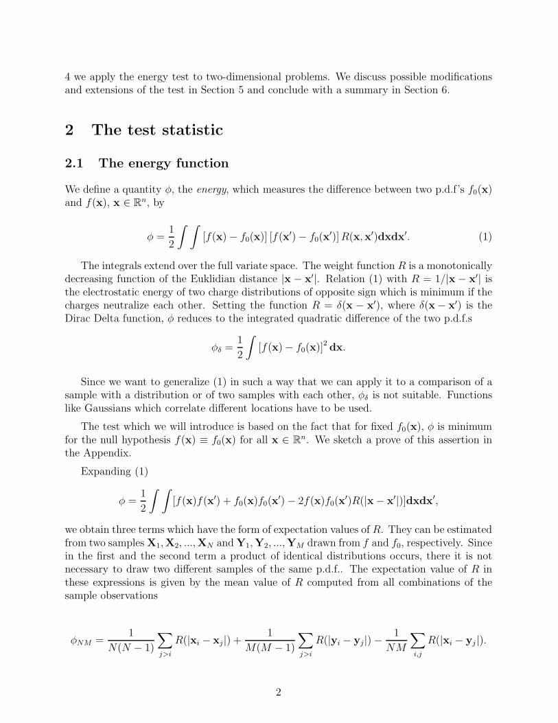
arXiv:hep-ex/0203010v5 29 Apr 2003 A new class of binning-free, multivariate goodness-of-fit tests: the energy tests ∗ B. Aslan and G. Zech † Universit¨at Siegen, D-57068 Siegen February 7, 2008 Abstract We present a new class of multivariate binning-free and nonparametric goodness- of-fit tests. The test quantity energy is a function of the distances of observed and simulated observations in the variate space. The simulation follows the probability distribution function f 0 of the null hypothesis. The distances are weighted with a weighting function which can be adjusted to the variations of f 0 . We have investigated the power of the test for a uniform and a Gaussian distribution of one or two variates, respectively and compared it to that of conventional tests. The energy test with a Gaussian weighting function is closely related to the Pearson χ 2 test but is more pow- erful in most applications and avoids arbitrary bin boundaries. The test is especially powerful in the multivariate case. 1 Introduction There exist a large number of binning-free goodness-of-fit tests for univariate distributions. The extension to the multivariate case is difficult, because there a natural ordering system is missing. The popular χ 2 test on the other hand suffers from the arbitrariness of the binning and from lack of power for small samples. The test proposed in this article avoids both, ordering and binning. It is especially powerful in the multivariate case. It is called energy test, because the definition of the test statistic is closely related to the energy of electric charge distributions. To facilitate the computation of the test statistic, we approximate the probability distribution function (p.d.f.) f 0 of the null hypothesis by simulated observations. The statistic “energy” can also be used to test whether two samples belong to the same parent distribution. In Section 2 we define the test and study its properties. Section 3 contains a comparison of the power of the energy test with that of other popular tests in one dimension. In Section * Supperted by Bunderministerium f¨ ur Bildung und Forschung, Deutschland † Corresponding author, email: [email protected] 1
-
Upload
independent -
Category
Documents
-
view
3 -
download
0
Transcript of A new class of binning free, multivariate goodness-of-fit tests: the energy tests
arX
iv:h
ep-e
x/02
0301
0v5
29
Apr
200
3
A new class of binning-free, multivariate goodness-of-fit
tests: the energy tests∗
B. Aslan and G. Zech†
Universitat Siegen, D-57068 Siegen
February 7, 2008
Abstract
We present a new class of multivariate binning-free and nonparametric goodness-of-fit tests. The test quantity energy is a function of the distances of observed andsimulated observations in the variate space. The simulation follows the probabilitydistribution function f0 of the null hypothesis. The distances are weighted with aweighting function which can be adjusted to the variations of f0. We have investigatedthe power of the test for a uniform and a Gaussian distribution of one or two variates,respectively and compared it to that of conventional tests. The energy test with aGaussian weighting function is closely related to the Pearson χ2 test but is more pow-erful in most applications and avoids arbitrary bin boundaries. The test is especiallypowerful in the multivariate case.
1 Introduction
There exist a large number of binning-free goodness-of-fit tests for univariate distributions.The extension to the multivariate case is difficult, because there a natural ordering system ismissing. The popular χ2 test on the other hand suffers from the arbitrariness of the binningand from lack of power for small samples.
The test proposed in this article avoids both, ordering and binning. It is especiallypowerful in the multivariate case. It is called energy test, because the definition of thetest statistic is closely related to the energy of electric charge distributions. To facilitatethe computation of the test statistic, we approximate the probability distribution function(p.d.f.) f0 of the null hypothesis by simulated observations. The statistic “energy” can alsobe used to test whether two samples belong to the same parent distribution.
In Section 2 we define the test and study its properties. Section 3 contains a comparisonof the power of the energy test with that of other popular tests in one dimension. In Section
∗Supperted by Bunderministerium fur Bildung und Forschung, Deutschland†Corresponding author, email: [email protected]
1
4 we apply the energy test to two-dimensional problems. We discuss possible modificationsand extensions of the test in Section 5 and conclude with a summary in Section 6.
2 The test statistic
2.1 The energy function
We define a quantity φ, the energy, which measures the difference between two p.d.f’s f0(x)and f(x), x ∈ R
n, by
φ =1
2
∫ ∫
[f(x) − f0(x)] [f(x′) − f0(x′)]R(x,x′)dxdx′. (1)
The integrals extend over the full variate space. The weight function R is a monotonicallydecreasing function of the Euklidian distance |x − x′|. Relation (1) with R = 1/|x − x′| isthe electrostatic energy of two charge distributions of opposite sign which is minimum if thecharges neutralize each other. Setting the function R = δ(x − x′), where δ(x − x′) is theDirac Delta function, φ reduces to the integrated quadratic difference of the two p.d.f.s
φδ =1
2
∫
[f(x) − f0(x)]2 dx.
Since we want to generalize (1) in such a way that we can apply it to a comparison of asample with a distribution or of two samples with each other, φδ is not suitable. Functionslike Gaussians which correlate different locations have to be used.
The test which we will introduce is based on the fact that for fixed f0(x), φ is minimumfor the null hypothesis f(x) ≡ f0(x) for all x ∈ R
n. We sketch a prove of this assertion inthe Appendix.
Expanding (1)
φ =1
2
∫ ∫
[f(x)f(x′) + f0(x)f0(x′) − 2f(x)f0(x
′)R(|x − x′|)]dxdx′,
we obtain three terms which have the form of expectation values of R. They can be estimatedfrom two samples X1,X2, ...,XN and Y1,Y2, ...,YM drawn from f and f0, respectively. Sincein the first and the second term a product of identical distributions occurs, there it is notnecessary to draw two different samples of the same p.d.f.. The expectation value of R inthese expressions is given by the mean value of R computed from all combinations of thesample observations
φNM =1
N(N − 1)
∑
j>i
R(|xi − xj |) +1
M(M − 1)
∑
j>i
R(|yi − yj|) −1
NM
∑
i,j
R(|xi − yj |).
2
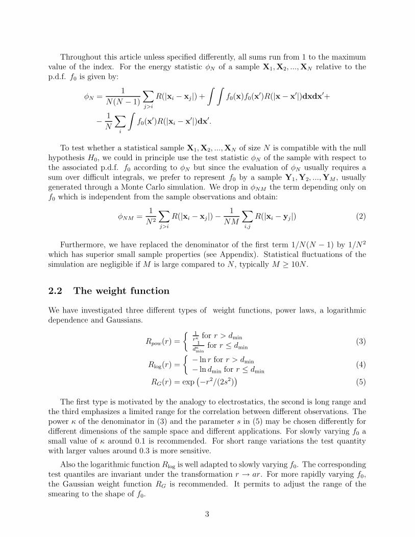
Throughout this article unless specified differently, all sums run from 1 to the maximumvalue of the index. For the energy statistic φN of a sample X1,X2, ...,XN relative to thep.d.f. f0 is given by:
φN =1
N(N − 1)
∑
j>i
R(|xi − xj |) +
∫ ∫
f0(x)f0(x′)R(|x − x′|)dxdx′+
−1
N
∑
i
∫
f0(x′)R(|xi − x′|)dx′.
To test whether a statistical sample X1,X2, ...,XN of size N is compatible with the nullhypothesis H0, we could in principle use the test statistic φN of the sample with respect tothe associated p.d.f. f0 according to φN but since the evaluation of φN usually requires asum over difficult integrals, we prefer to represent f0 by a sample Y1,Y2, ...,YM , usuallygenerated through a Monte Carlo simulation. We drop in φNM the term depending only onf0 which is independent from the sample observations and obtain:
φNM =1
N2
∑
j>i
R(|xi − xj |) −1
NM
∑
i,j
R(|xi − yj|) (2)
Furthermore, we have replaced the denominator of the first term 1/N(N − 1) by 1/N2
which has superior small sample properties (see Appendix). Statistical fluctuations of thesimulation are negligible if M is large compared to N , typically M ≥ 10N .
2.2 The weight function
We have investigated three different types of weight functions, power laws, a logarithmicdependence and Gaussians.
Rpow(r) =
{
1rκ
for r > dmin1
dκ
min
for r ≤ dmin(3)
Rlog(r) =
{
− ln r for r > dmin
− ln dmin for r ≤ dmin
(4)
RG(r) = exp(
−r2/(2s2))
(5)
The first type is motivated by the analogy to electrostatics, the second is long range andthe third emphasizes a limited range for the correlation between different observations. Thepower κ of the denominator in (3) and the parameter s in (5) may be chosen differently fordifferent dimensions of the sample space and different applications. For slowly varying f0 asmall value of κ around 0.1 is recommended. For short range variations the test quantitywith larger values around 0.3 is more sensitive.
Also the logarithmic function Rlog is well adapted to slowly varying f0. The correspondingtest quantiles are invariant under the transformation r → ar. For more rapidly varying f0,the Gaussian weight function RG is recommended. It permits to adjust the range of thesmearing to the shape of f0.
3
The inverse power law and the logarithm exhibit a pole at r equal to zero which couldproduce infinities in the double discrete version of the energy function φNM . Very smalldistances, however, should not be weighted too strongly since deviations from f0 with sharppeaks are not expected and usually inhibited by the finite experimental resolution. Weeliminate the poles by introducing a lower cutoff dmin for the distances r. Distances less thandmin are replaced by dmin. The value of this parameter is not critical at all, it should be of theorder of the average distance of the simulation points in the region where f0 is maximum.
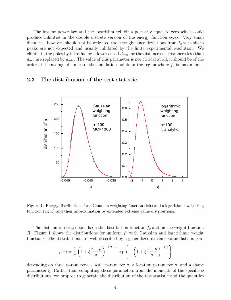
2.3 The distribution of the test statistic
-0.045 -0.040 -0.0350
50
100
150
200
250 Gaussianweightingfunction
n=100MC=1000
dist
ribut
ion
of f
f
-2 -1 0 1 2 30.0
0.1
0.2
0.3
0.4
0.5
0.6 logarithmicweightingfunction
n=100f0 analytic
f
Figure 1: Energy distributions for a Gaussian weighting function (left) and a logarithmic weighting
function (right) and their approximation by extended extreme value distributions.
The distribution of φ depends on the distribution function f0 and on the weight functionR. Figure 1 shows the distributions for uniform f0 with Gaussian and logarithmic weightfunctions. The distributions are well described by a generalized extreme value distribution
f(x) =1
σ
(
1 + ξx− µ
σ
)
−1/ξ−1
exp
{
−
(
1 + ξx− µ
σ
)
−1/ξ}
depending on three parameters, a scale parameter σ, a location parameter µ, and a shapeparameter ξ. Rather than computing these parameters from the moments of the specific φdistributions, we propose to generate the distribution of the test statistic and the quantiles
4

by a Monte Carlo simulation. As a consequence of the dramatic increase of computingpower during the last decade, it has become possible to perform the calculations on a simplePC within minutes. There is no need to publish tables of percentage points, to distinguishbetween simple and composite hypotheses and also censoring can be incorporated into thesimulation.
2.4 Relation to the Pearson χ2 test
Let us assume that we have in a certain χ2-bin ni experimental observations and mi MonteCarlo observations and β = M/N ≫ 1. Then the χ2 contribution of that bin is
χ2i =
(ni −mi/β)2
mi/β
=n2
i − 2nimi/β +m2i /β
2
mi/β
For a goodness-of-fit test, an additive constant is irrelevant. Thus we can drop m2i in the
last relation. If in addition the theoretical distribution is uniform and the bins have constantsize, we can also ignore the denominator.
χ2′i =
n2i
2−nimi
β
Up to a constant factor this last relation corresponds nearly to the energy defined in (2) fora weight function which is constant inside the bin and zero outside:
φNM =ni(ni − 1)
2N2−nimi
NM≈
1
N2χ2′
i
The χ2 test applied to a uniform distribution f0 is equivalent to an energy test with abox shaped weight function and fixed box locations.
Replacing the box function by the Gaussian weight function, the sharp cut at the binboundaries and the arbitrary location of the boundary for fixed binning are avoided but theidea underlying the χ2 test is retained.
2.5 Optimization of the test parameters in a simple case
To study the dependence of the power of the test on the choice of the weight function andits parameters, we have chosen for H0 a uniform, univariate p.d.f. f0 restricted to the unitinterval [0, 1]. We determined the rejection power with respect to contaminations of f0 witha linear and two different Gaussian distributions which represent a wide and a more localdistortion.
f0 = 1
f1(X) = 2X (6)
f2(X) = c2 exp(
−64(X − 0.5)2)
(7)
f3(X) = c3 exp(
−256(X − 0.5)2)
(8)
5
We required 5% significance level and computed the rejection power which is equal to oneminus the probability for an error of the second kind.
As a reference, we also computed the power of a χ2 test with bins of fixed width. Thenumber of bins B ≈ 2N2/5 was chosen according to the prescription proposed in [5].
The cut-off parameter dmin for Rκ (power law) and Rl (logarithmic) was set equal to1/(4N).
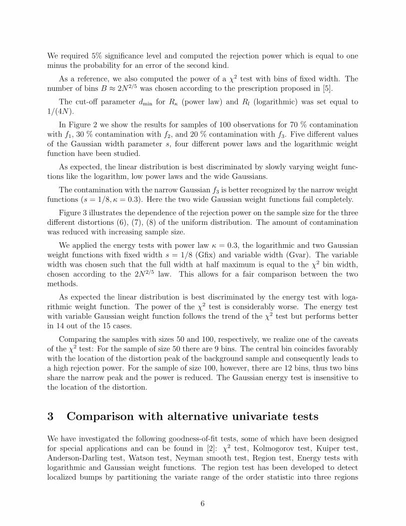
In Figure 2 we show the results for samples of 100 observations for 70 % contaminationwith f1, 30 % contamination with f2, and 20 % contamination with f3. Five different valuesof the Gaussian width parameter s, four different power laws and the logarithmic weightfunction have been studied.
As expected, the linear distribution is best discriminated by slowly varying weight func-tions like the logarithm, low power laws and the wide Gaussians.
The contamination with the narrow Gaussian f3 is better recognized by the narrow weightfunctions (s = 1/8, κ = 0.3). Here the two wide Gaussian weight functions fail completely.
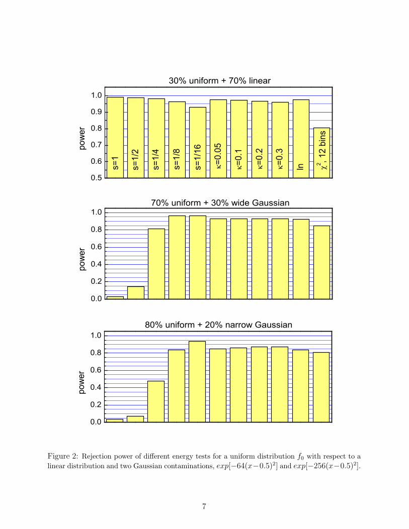
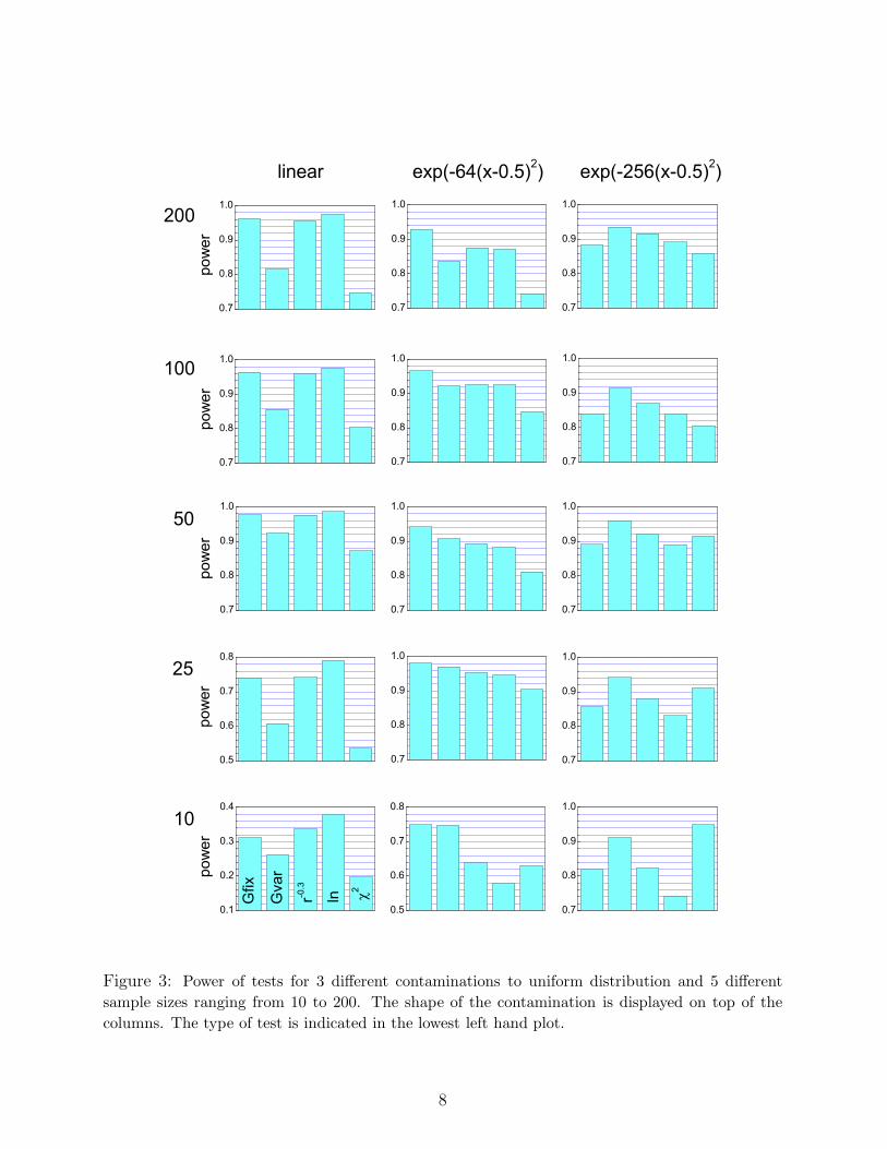
Figure 3 illustrates the dependence of the rejection power on the sample size for the threedifferent distortions (6), (7), (8) of the uniform distribution. The amount of contaminationwas reduced with increasing sample size.
We applied the energy tests with power law κ = 0.3, the logarithmic and two Gaussianweight functions with fixed width s = 1/8 (Gfix) and variable width (Gvar). The variablewidth was chosen such that the full width at half maximum is equal to the χ2 bin width,chosen according to the 2N2/5 law. This allows for a fair comparison between the twomethods.
As expected the linear distribution is best discriminated by the energy test with loga-rithmic weight function. The power of the χ2 test is considerably worse. The energy testwith variable Gaussian weight function follows the trend of the χ2 test but performs betterin 14 out of the 15 cases.
Comparing the samples with sizes 50 and 100, respectively, we realize one of the caveatsof the χ2 test: For the sample of size 50 there are 9 bins. The central bin coincides favorablywith the location of the distortion peak of the background sample and consequently leads toa high rejection power. For the sample of size 100, however, there are 12 bins, thus two binsshare the narrow peak and the power is reduced. The Gaussian energy test is insensitive tothe location of the distortion.
3 Comparison with alternative univariate tests
We have investigated the following goodness-of-fit tests, some of which have been designedfor special applications and can be found in [2]: χ2 test, Kolmogorov test, Kuiper test,Anderson-Darling test, Watson test, Neyman smooth test, Region test, Energy tests withlogarithmic and Gaussian weight functions. The region test has been developed to detectlocalized bumps by partitioning the variate range of the order statistic into three regions
6
0.0
0.2
0.4
0.6
0.8
1.0
powe
r
0.5
0.6
0.7
0.8
0.9
1.0
k=0.
05
80% uniform + 20% narrow Gaussian
70% uniform + 30% wide Gaussian
30% uniform + 70% linear
c2 , 12
bins
lnk=0.
3
k=0.
2
k=0.
1
s=1/
16
s=1/
8
s=1/
4
s=1/
2
s=1
po
wer
0.0
0.2
0.4
0.6
0.8
1.0
powe
r
Figure 2: Rejection power of different energy tests for a uniform distribution f0 with respect to a
linear distribution and two Gaussian contaminations, exp[−64(x−0.5)2] and exp[−256(x−0.5)2].
7
0.7
0.8
0.9
1.0
pow
er
0.7
0.8
0.9
1.0
0.7
0.8
0.9
1.0
0.7
0.8
0.9
1.0
pow
er
0.7
0.8
0.9
1.0
linear exp(-64(x-0.5)2) exp(-256(x-0.5)2)
0.7
0.8
0.9
1.0
0.7
0.8
0.9
1.0
pow
er
0.7
0.8
0.9
1.0
0.7
0.8
0.9
1.0
0.1
0.2
0.3
0.4
c2
lnr-0.3
Gva
r
Gfix
pow
er
0.5
0.6
0.7
0.8
0.7
0.8
0.9
1.010
25
50
100
200
0.5
0.6
0.7
0.8
pow
er
0.7
0.8
0.9
1.0
0.7
0.8
0.9
1.0
Figure 3: Power of tests for 3 different contaminations to uniform distribution and 5 different
sample sizes ranging from 10 to 200. The shape of the contamination is displayed on top of the
columns. The type of test is indicated in the lowest left hand plot.
8
B
C
A
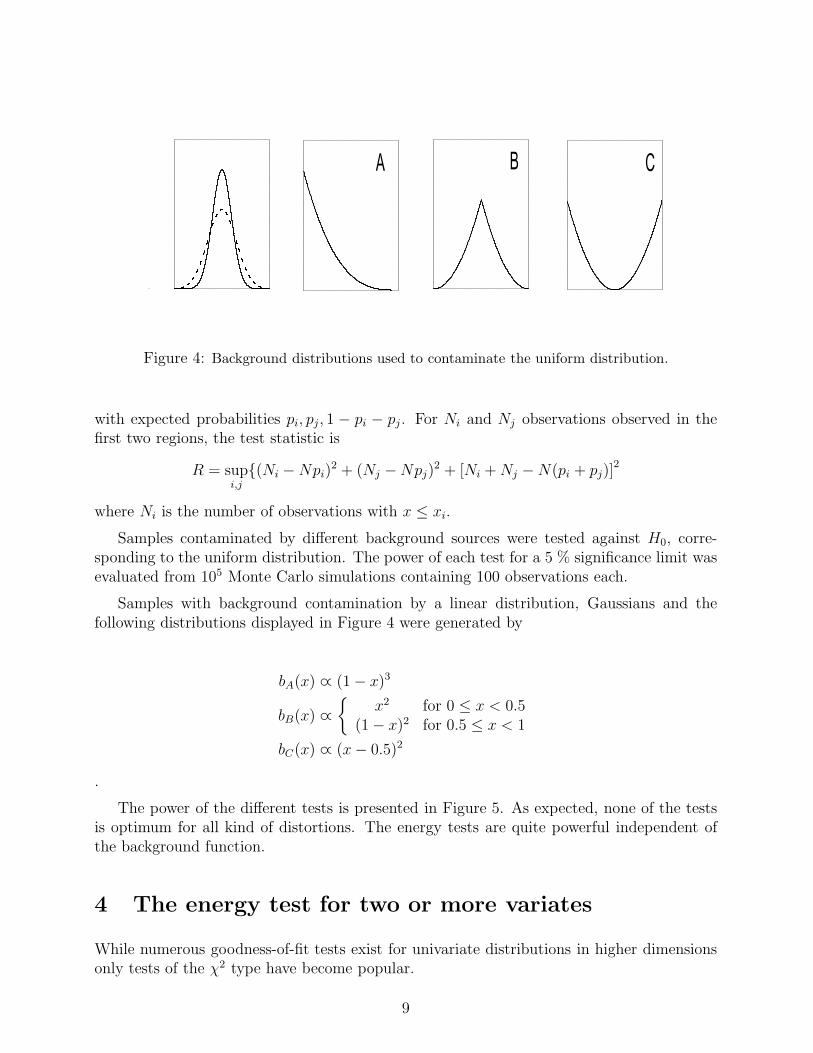
Figure 4: Background distributions used to contaminate the uniform distribution.
with expected probabilities pi, pj, 1 − pi − pj . For Ni and Nj observations observed in thefirst two regions, the test statistic is
R = supi,j
{(Ni −Npi)2 + (Nj −Npj)
2 + [Ni +Nj −N(pi + pj)]2
where Ni is the number of observations with x ≤ xi.
Samples contaminated by different background sources were tested against H0, corre-sponding to the uniform distribution. The power of each test for a 5 % significance limit wasevaluated from 105 Monte Carlo simulations containing 100 observations each.
Samples with background contamination by a linear distribution, Gaussians and thefollowing distributions displayed in Figure 4 were generated by
bA(x) ∝ (1 − x)3
bB(x) ∝
{
x2
(1 − x)2
for 0 ≤ x < 0.5for 0.5 ≤ x < 1
bC(x) ∝ (x− 0.5)2
.
The power of the different tests is presented in Figure 5. As expected, none of the testsis optimum for all kind of distortions. The energy tests are quite powerful independent ofthe background function.
4 The energy test for two or more variates
While numerous goodness-of-fit tests exist for univariate distributions in higher dimensionsonly tests of the χ2 type have become popular.
9

50% linear 30% A 30% C 0.0
0.5
1.0
pow
er
Anderson Kolmogorov Kuiper Neyman Watson Region Energy(log) Energy1(Gaussian) Chi
30% B 20% N(0.5,1/24) 20% N(0.5,1/32)0.0
0.5
1.0
pow
er
Figure 5: Rejection power of tests with respect to different contaminations to the uniform distri-
bution. The contaminations correspond to the distributions shown in the previous figure.
10
The extension of binning-free tests based on linear rank statistics to the multivariatecase [3] is difficult because no obvious ordering scheme of the observations exist. Sequentialordering in the different variates depends on the sequence in which the variates are chosen.In addition to this logical difficulty there is a more fundamental problem: The re-shufflingof the observations destroys the natural metric used to display the data. The situation ingoodness-of-fit problems is very similar to that in pattern recognition. The possibility todetect distortions of the expected distribution by background or resolution effects dependson an appropriate selection of the random variables. The natural choice is usually givenby the experiment. By mapping a multivariate space onto a space defined by the orderingrecipe much of the information contained in the original distribution may be lost.
4.1 Test for bivariate Gaussian distribution
It is rather common to deal with samples of observations which are drawn from a multivariatenormality. Multivariate goodness-of-fit tests have been developed mostly for multinormality.An overview can be found in [1]. An extension of the moment tests introduced by K.Pearson to two variates is Mardia’s test [4]. Skewness β1 and kurtosis β2 are compared tothe nominal values for the normal distribution, β1 = 0 and β2 = 3 respectively. We comparedthe logarithmic and the Gaussian energy tests to Mardia’s tests and to the two-dimensionalNeyman smooth test [7].
We chose a standard Gaussian
f0 =1
2πexp
(
−(x2 + y2)/2)
to represent the null hypothesis.
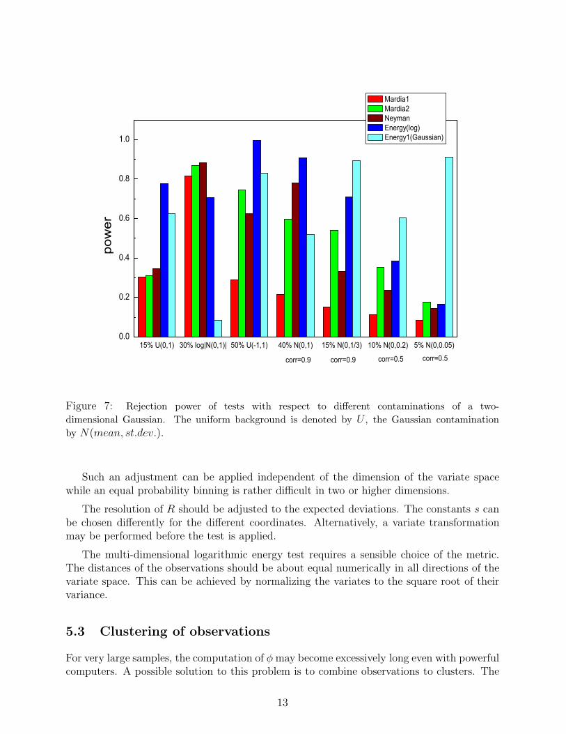
Background samples added to f0 are shown in Figure 6. In addition, a uniform back-ground in the region (0 < X, Y < 1) and variations of the Gaussian background wereinvestigated. All Gaussians have the same width in both coordinates X and Y , but differ inthe value of the width and the correlation coefficient.
Figure 7 displays the results. We were astonished how well the energy test competes withalternatives especially designed to test normality. We attribute the excellent performance ofthe energy test to the fact that it is sensitive to all deviations of two distributions whereasthe Mardia tests are based only on two specific moments.
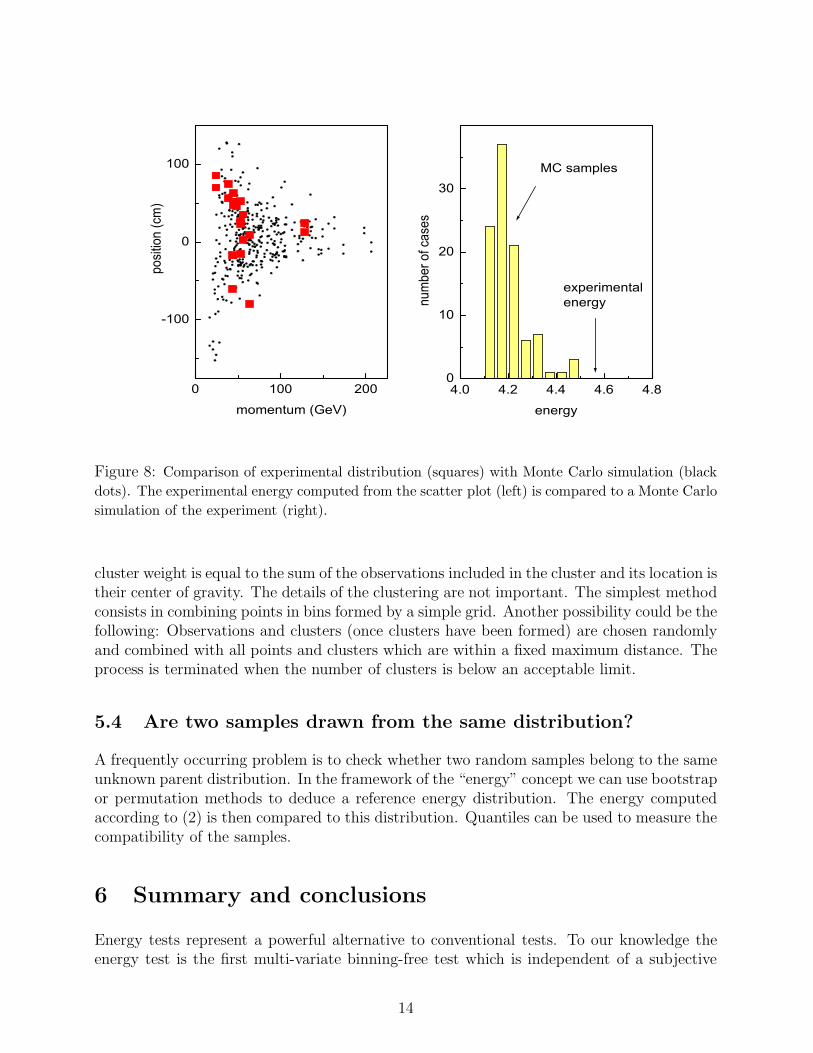
4.2 Example from particle physics
Figure 8 is a scatter plot of data obtained in the particle physics experiment HERA-B atDESY. The positions of tracks from ψ decays are plotted against the momentum of the ψmeson. The 20 square entries represent the experimental data, the black dots correspond toa Monte Carlo simulation.
We have computed the energy statistic φ with the logarithmic weighting function forthe experimental data relative to the Monte Carlo prediction. Separately, the energy wasdetermined for 100 independent Monte Carlo samples of 20 events each to estimate the
11

-3 0 3
-3
0
3
-6 -4 -2 0 2-6
-4
-2
0
2
y
x
N(0,1)corr=0.9
y
x
log|N(0,1)|
Figure 6: Background distributions used to contaminate a two-dimensional Gaussian.
distribution of φ under H0. The experimental value is larger than all Monte Carlo values(see Figure 8), indicating that the data do not follow the prediction.
5 Extensions and variations of the energy test
5.1 Normalization to probability density
The Gaussian energy test has proven to be similar but superior to the χ2 test for the uniformdistribution. For non-uniform p.d.f.s the similarity can be retained by effectively dividingthe elements of the sums in (2) by the p.d.f. f0.
R(|xi − xj |) → R′(|xi − xj |) =R(|xi − xj|)√
f0(xi)f0(xj)
If the density is only given by a Monte Carlo simulation, the density can be estimated fromthe volume of a multidimensional sphere in the variate space containing a fixed number ofMonte Carlo observations. In the example of Figure 8 the density at x could be estimatedfrom the area A(x) of the smallest circle centered at x containing 10 Monte Carlo points:f0(x) ≈ 10/A(x).
5.2 Width of the weighting function R and metric
Some statisticians recommend to use equal probability bins for the χ2 test in one dimension.An equivalent procedure for the Gaussian energy test would be to adjust the width of theGaussian weighting function to the p.d.f.
Rs(rij) → R′
s(rij) = exp(
−r2/(2sisj))
si ∝ 1/f0(xi)
12
15% U(0,1) 30% log|N(0,1)| 50% U(-1,1) 40% N(0,1) 15% N(0,1/3) 10% N(0,0.2) 5% N(0,0.05)0.0
0.2
0.4
0.6
0.8
1.0
p
ower
corr=0.5corr=0.5corr=0.9corr=0.9
Mardia1 Mardia2 Neyman Energy(log) Energy1(Gaussian)
Figure 7: Rejection power of tests with respect to different contaminations of a two-
dimensional Gaussian. The uniform background is denoted by U , the Gaussian contamination
by N(mean, st.dev.).
Such an adjustment can be applied independent of the dimension of the variate spacewhile an equal probability binning is rather difficult in two or higher dimensions.
The resolution of R should be adjusted to the expected deviations. The constants s canbe chosen differently for the different coordinates. Alternatively, a variate transformationmay be performed before the test is applied.
The multi-dimensional logarithmic energy test requires a sensible choice of the metric.The distances of the observations should be about equal numerically in all directions of thevariate space. This can be achieved by normalizing the variates to the square root of theirvariance.
5.3 Clustering of observations
For very large samples, the computation of φmay become excessively long even with powerfulcomputers. A possible solution to this problem is to combine observations to clusters. The
13
0 100 200
-100
0
100
4.0 4.2 4.4 4.6 4.80
10
20
30MC samples
experimentalenergy
num
ber o
f cas
esenergy
posit
ion
(cm
)
momentum (GeV)
Figure 8: Comparison of experimental distribution (squares) with Monte Carlo simulation (black
dots). The experimental energy computed from the scatter plot (left) is compared to a Monte Carlo
simulation of the experiment (right).
cluster weight is equal to the sum of the observations included in the cluster and its location istheir center of gravity. The details of the clustering are not important. The simplest methodconsists in combining points in bins formed by a simple grid. Another possibility could be thefollowing: Observations and clusters (once clusters have been formed) are chosen randomlyand combined with all points and clusters which are within a fixed maximum distance. Theprocess is terminated when the number of clusters is below an acceptable limit.
5.4 Are two samples drawn from the same distribution?
A frequently occurring problem is to check whether two random samples belong to the sameunknown parent distribution. In the framework of the “energy” concept we can use bootstrapor permutation methods to deduce a reference energy distribution. The energy computedaccording to (2) is then compared to this distribution. Quantiles can be used to measure thecompatibility of the samples.
6 Summary and conclusions
Energy tests represent a powerful alternative to conventional tests. To our knowledge theenergy test is the first multi-variate binning-free test which is independent of a subjective
14
ordering system. With a logarithmic weighting function it is very sensitive to long range dis-tortions of the distribution to be tested, a situation which is frequent in physics applications.With a Gaussian weighting function the energy test has similar properties as tests of the χ2
type, but avoids arbitrary bin boundaries. It is more powerful than the χ2 test in almostall cases which we have considered. It can cope with arbitrarily small sample sizes. It isastonishing how well the energy test can compete with the Mardia test for testing normalityin two dimensions.
The necessity to determine the distribution function of the test statistic for the specificapplication is not a serious restriction with today’s computing power.
The energy statistic can be used to test whether different samples belong to the sameparent distribution. A corresponding study will be presented in a forthcoming article.
7 Appendix
7.1 Continuous case
We conjecture that f(x) ≡ f0(x) corresponds to a minimum of φ in (1). Substitutingg(x) = f(x) − f0(x) we obtain
φ =1
2
∫ ∫
g(x)g(x′)R(|x − x′|)dxdx′ ≥ 0 (9)
where g fulfils the condition∫
g(x)dx = 0. We conjecture that φ is minimum for g(x) ≡ 0for weight functions R which decrease continuously with |x − x′|.
In the following, we sketch a prove of this conjecture without full mathematical rigor andgenerality.
The property (9) is invariant under a linear transformation
R → R′ = αR+ const
where α is a positive scaling factor. Assuming that R is finite, we can restrict its values tothe range −1 ≤ R ≤ 1 with R(0) = 1. We approximate the function g by a histogram withfunction value gi in bin i. The size of each bin is ∆n.
φh = ∆2n∑
i,j
gigjRij
with self-explaining notation. The weights can be substituted by cosines, cos θij = Rij withcos θii = 1 in our approximation. The sum then can be written as a sum of vectors gi in R
n:
φh = ∆2n∑
i,j
gigj cos θij
φh = ∆2n
(
∑
i
gi
)2
≥ 0
The minimum of φh is realized only if all gi are equal to zero.
15
7.2 Discrete case
When we approximate both densities f and f0 by distributions ofN points each, with weightsequal 1/N , we require that the energy be minimum if the two samples coincide, xj = yj ∀j.To fulfil this condition, we have to replace the factors 1/(N − 1) and 1/(M − 1) by 1/N inφNM .
φNN =1
N2
∑
j>i
R(|xi − xj |) +1
N2
∑
j>i
R(|yi − yj |)+
−1
N2
∑
i,j
R(|xi − yj|)
To demonstrate the minimum condition which leads to φNN = 0, we apply an infinitesimalshift to one observation. For xj = yj for j 6= k and xk − yk = δxk, only the pair xk,yk
contributes to the energy, all other terms cancel.
φNN = −1
N2[R(|δxk| − R(0)]
Since R decreases with its argument, R(0) − R(|δxk|) > 0, we have found a local minimum
of the energy.
For the special choice where R is the distance function, i. e. increasing with the distance,it has been demonstrated by [6] that φ
φ =1
N2
∑
j>i
[|xi − xj| + |yi − yj |] −1
N2
∑
i
∑
j
|xi − yj| ≤ 0
is maximum for xj = yj for all j. Since φ is constant for constant R, it is plausible that fordiscrete distributions φ is minimum for xj = yj for all decreasing functions of the distance,and maximum for all increasing functions of the distance, however, we did not succeed infinding a general prove of this conjecture.
Acknowledgments. The authors wish to express their gratitude to Prof. R.-D. Reissfor his constructive comments on earlier drafts of this paper, which led to improvements inthe presentation.
References
[1] D’Agostino, R.B. (1986), “Tests for the Normal Distribution,” In Goodness-of-Fit Tech-
niques (eds D’Agostino, R.B. and Stephens, M.A.), pp. 367-419, New York: Dekker.
[2] D’Agostino, R.B., and Stephens, M.A. (1986), Goodness-of-Fit Techniques, New York:Dekker.
[3] Justel, A., Pena, D., and Zamar, R. (1997), “A multivariate Kolmogorov-Smirnov testof goodness of fit,” Statistics & Probability Letters, 35, 251-259.
16
[4] Mardia, V.K. (1970), “Measures of multivariate skewness and kurtosis with applica-tions,” Biometrica, 57, 519-530.
[5] Moore, D.S. (1986), “Tests of Chi Squared Type,” In Goodness-of-Fit Techniques (edsD’Agostino, R.B. and Stephens, M.A.), pp. 63-95, New York: Dekker.
[6] Morgenstern, D. (2002), “Proof of a conjecture by Walter Deuber concerning the dis-tance between points of two types in R
d,” Discrete Mathematics, 226, 347-.
[7] Rayner, J.C.W., and Best, D.J. (1986), Smooth Tests of Goodness of Fit, Oxford: OxfordUniversity Press.
17