Binning sequences using very sparse labels within a metagenome

BioMed CentralBMC Bioinformatics

ss
Open AcceMethodology articleBinning sequences using very sparse labels within a metagenomeChon-Kit Kenneth Chan1, Arthur L Hsu1, Saman K Halgamuge1 and Sen-Lin Tang*2
Address: 1Dynamic Systems & Control Group, Department of Mechanical Engineering, The University of Melbourne, Australia and 2Research Centre for Biodiversity, Academia Sinica, Taipei, Taiwan

Email: Chon-Kit Kenneth Chan - [email protected]; Arthur L Hsu - [email protected]; Saman K Halgamuge - [email protected]; Sen-Lin Tang* - [email protected]

* Corresponding author

AbstractBackground: In metagenomic studies, a process called binning is necessary to assign contigs that belongto multiple species to their respective phylogenetic groups. Most of the current methods of binning, suchas BLAST, k-mer and PhyloPythia, involve assigning sequence fragments by comparing sequence similarityor sequence composition with already-sequenced genomes that are still far from comprehensive. Wepropose a semi-supervised seeding method for binning that does not depend on knowledge of completedgenomes. Instead, it extracts the flanking sequences of highly conserved 16S rRNA from the metagenomeand uses them as seeds (labels) to assign other reads based on their compositional similarity.

Results: The proposed seeding method is implemented on an unsupervised Growing Self-Organising Map(GSOM), and called Seeded GSOM (S-GSOM). We compared it with four well-known semi-supervisedlearning methods in a preliminary test, separating random-length prokaryotic sequence fragments sampledfrom the NCBI genome database. We identified the flanking sequences of the highly conserved 16S rRNAas suitable seeds that could be used to group the sequence fragments according to their species. S-GSOMshowed superior performance compared to the semi-supervised methods tested. Additionally, S-GSOMmay also be used to visually identify some species that do not have seeds.

The proposed method was then applied to simulated metagenomic datasets using two different confidencethreshold settings and compared with PhyloPythia, k-mer and BLAST. At the reference taxonomic levelOrder, S-GSOM outperformed all k-mer and BLAST results and showed comparable results withPhyloPythia for each of the corresponding confidence settings, where S-GSOM performed better thanPhyloPythia in the ≥ 10 reads datasets and comparable in the ≥ 8 kb benchmark tests.

Conclusion: In the task of binning using semi-supervised learning methods, results indicate S-GSOM tobe the best of the methods tested. Most importantly, the proposed method does not require knowledgefrom known genomes and uses only very few labels (one per species is sufficient in most cases), which areextracted from the metagenome itself. These advantages make it a very attractive binning method. S-GSOM outperformed the binning methods that depend on already-sequenced genomes, and compareswell to the current most advanced binning method, PhyloPythia.

Published: 28 April 2008

BMC Bioinformatics 2008, 9:215 doi:10.1186/1471-2105-9-215

Received: 23 October 2007Accepted: 28 April 2008

This article is available from: http://www.biomedcentral.com/1471-2105/9/215

© 2008 Chan et al; licensee BioMed Central Ltd. This is an Open Access article distributed under the terms of the Creative Commons Attribution License (http://creativecommons.org/licenses/by/2.0), which permits unrestricted use, distribution, and reproduction in any medium, provided the original work is properly cited.

of 17(page number not for citation purposes)

http://www.ncbi.nlm.nih.gov/entrez/query.fcgi?cmd=Retrieve&db=PubMed&dopt=Abstract&list_uids=18442374

http://www.biomedcentral.com/1471-2105/9/215

http://creativecommons.org/licenses/by/2.0

http://www.biomedcentral.com/

http://www.biomedcentral.com/info/about/charter/

BMC Bioinformatics 2008, 9:215 http://www.biomedcentral.com/1471-2105/9/215

BackgroundWith the advancement of technology, genome sequencingprojects are moving from the study of single genomes tothe examination of genomes in a community. This newstudy, metagenomics, allows culture-independent andsequence-based studies of microbial communities. Ametagenomic project generally starts by using WholeGenome Shotgun (WGS) sequencing [1-6] on environ-mental samples to acquire sequence reads, followed byassembling sequence reads, gene prediction, functionalannotation and metabolic pathway construction. A neces-sary step in metagenomics, which is not required in singlegenome sequencing, is called binning. The binning proc-ess sorts contigs and scaffolds of multiple species,obtained from WGS sequencing, into phylogeneticallyrelated groups (bins). The resolution of phylogeneticgrouping can vary from high levels such as domain, downto low levels such as strain of a given microorganism,depending on a number of factors such as the binningmethod used, community structure and sequencing qual-ity and depth [7]. As the community structure is inherentin the nature of the environmental sample collected, andsequencing quality and depth rely heavily on the sequenc-ing technology and sample size, the major focus of com-putational techniques is on the method of binning.

A number of binning methods are currently available thatfall into two broad categories: sequence similarity-basedand sequence composition-based. Sequence similarity-based binning methods, for example BLAST, classifysequences based on the distribution of BLAST hits of pre-dicted genes to taxonomic classes. Composition-basedmethods discriminate genomes by analysing the intrinsicfeatures of sequence encoding preferences, such as GCcontent [8], codon usage [9] or oligonucleotide frequen-cies [10-12], for different genomes. Different approachesto extracting sequence features have been proposed. Somecomposition-based binning methods include k-mer [11],oligonucleotide-frequency-based clustering with Self-Organising Maps (SOM) [13,14], PhyloPythia [15] andTETRA [16,17], all of which have yielded promisingresults. The k-mer method calculates the oligonucleotidefrequencies of all sequence fragments and compares themto a reference set of completed genomes. Clustering of oli-gonucleotide frequencies with SOM can be used in twodifferent ways: directly clustering the metagenomic sam-ple sequences using different oligonucleotide frequenciesas features [13], or building an SOM classifier usingsequences in existing databases and then assigningmetagenomic samples to the closest matching node in theclassifier [14]. PhyloPythia follows a similar approach tothe SOM classifier method, building a classificationmodel from the sequenced genomes and assigning sam-ple sequences to phylogenetic clades according to the sim-ilarity of metagenomic sequence patterns. Two types of

PhyloPythia models can be built, a generic model and asample-specific model. The generic model is constructedusing the sequence patterns of a reference set of isolatedgenomes and the sample-specific model includes addi-tional marker-gene labelled sequence fragments (around100 kb length) from each of the dominant population ofthe sample. In contrast, TETRA follows the SOM clusteringapproach that does not require reference genomes. It binsthe species-specific sequences by comparing the pairwisetetranucleotide-derived z-score correlations of everysequence.

The above named binning methods can be divided, froma machine learning perspective, into supervised and unsu-pervised learning methods. Methods that build a classifierusing the knowledge of completed genomes belong to theclass of supervised learning methods, such as BLAST, k-mer and the SOM classifier approach. However, consider-ing the current amount of known genomes, which isinsufficient to represent the almost limitless microbialgenomes [18], the resultant under-representation of train-ing samples can be detrimental to these supervised-learn-ing methods. PhyloPythia, being the latest of the binningmethods addressed here, has been shown to be able toclassify sequence reads with great accuracy when trainingdata is highly relevant to the species being assigned, whichcan either be from a set of reference genomes or using 100kb length marker-gene labelled sequences, which may notalways exist to build a sample-specific model. Unsuper-vised-learning methods do not have this dependence ontraining data. TETRA falls into this category, but it focuseson the long fosmid-sized 40 kb fragments and its all-verse-all pairwise comparison matrix can quickly becomeintractable for a large number of sequences. The directclustering approach with SOM was tested to separate 1 kband 10 kb sequence fragments derived from 65 bacteriaand 6 eukaryotes, but only the 10 kb tests showed clearspecies-specific separations [13]. Nevertheless, withoutthe reference sequences, the results lack identifiable labelsto resolve for the clusters of sequence reads produced.

To circumvent dependence on the knowledge of com-pleted genomes and provide meaningful clusteringresults, we propose a semi-supervised seeding algorithmthat uses very small amounts of labelled samples,extracted from metagenomes, for binning metagenomicsequences. The seeding method is a post-processingmethod that can be applied to an unsupervised clusteringalgorithm of choice, for example, SOM, Growing Self-Organising Maps (GSOM) [19], or the Incremental GridGrowing Neural Network [20], which also provide dimen-sionality reduction for data visualisation. Comparing theclustering qualities of SOM and GSOM indicated thatGSOM has a better clustering quality and faster computa-



tional speed, as confirmed by experiments conducted onother datasets [21,22].

Therefore, in this paper, we implemented the proposedseeding method on GSOM, henceforth abbreviated as S-GSOM. The performance of S-GSOM for binning metage-nomic sequences is demonstrated by applying it to simu-lated metagenomic datasets. Preliminary tests were firstconducted to compare S-GSOM with the following well-known semi-supervised learning methods: Constraint-Partitioning K-Means (COP K-Means), Constrained K-Means, Seeded K-Means and the Transductive SupportVector Machine (TSVM) on the task of separatingsequence fragments created from 10, 20 and 40 prokaryo-tic species randomly sampled from the NCBI genomedatabase. For a comparison with current binning meth-ods, further tests of S-GSOM were performed using therecently published simulated metagenomic datasets thatwere created to evaluate the fidelity of metagenomicprocessing methods [7].

MethodsDatasets preparation and data pre-processing for separation of prokaryotic DNA sequencesGeneration of independent simulated metagenomic dataThe most updated NCBI database contains 488 completedArchaea/Bacteria genomes [23]. Genome sequences of 10,20 and 40 species were randomly selected from the NCBIdatabase. In total, seven random sets were independentlydrawn from the database, replacing them each time. Threesets were drawn for each of the 10 and 20 species datasetsand only one set for the 40 species dataset, considering thelimitations imposed by the available computingresources. (For computational time estimation withoutthe seeding procedure, please refer to our previous publi-cation [22]). For convenience, we abbreviated the datasetscreated in the form of 'XSp-SetY' where 'X' denotesnumber of species and 'Y' represents the number in thedraw. For example, the first dataset containing 10 randomspecies is denoted by the abbreviation '10Sp-Set1' and the

other datasets are named in the same manner. The lists ofspecies in all datasets can be found in supplementarymaterial [see Additional file 1].

The first step in pre-processing involves the extraction offragments from the collected datasets. Since rRNA andtRNA sequences are very similar among different species[24], they are likely to interfere with the clustering processwhen nucleotide frequencies are used as training features.Therefore, we take the precaution to reduce noise byavoiding the inclusion of these RNA sequences. This noisereduction is also valid in practical situations because allthese RNA sequences can be easily identified based onsequence similarity against public databases, e.g. RDP[25] or GenBank [23], and are excluded from the cluster-ing process. Figure 1 contains an example for preparingunlabelled input vectors and seeds for clustering algo-rithms, and a typical extraction process is as follows:

1. Identify all rRNA and tRNA sequences in the genome.

2. Obtain 8–13 kb length seeding sequences that flank the16S rRNA sequence (see later for more details on seedingsequences). Ensure that a seeding sequence does not over-lap other rRNA and tRNA sequences.

3. Remove all rRNA, tRNA and seeding sequences fromthe genome to obtain initial sequence fragments.

4. Divide initial sequence fragments into non-overlapping8–13 kb (determined randomly) length fragments. Frag-ments shorter than 8 kb are discarded.

5. Nucleotide frequencies of each sequence fragments arecomputed using a sliding window of the size of 4 bases(tetranucleotide frequencies). A total of 256 (44) combi-nations of nucleotide usages are represented in the vectorform of 256 dimensions.

An example for preparing unlabelled input vectors and seedsFigure 1An example for preparing unlabelled input vectors and seeds. Unlabelled input vectors and seeds are prepared by avoiding the RNA sequences.



6. Since the sequences were cut into random lengthsbetween 8 kb and 13 kb fragments, the tetranucleotide fre-quencies also need to be normalised relative to the lengthof the fragments (i.e. frequency per base).

The choice to use 8 kb as the minimum sequence length isbecause the number of chimeric sequences becomes sig-nificant for sequence length < 8 kb using the currentlyavailable assemblers [7], and the chimeric sequences willreduce the binning accuracy leading to meaninglessresults. The same reason explains the use of ≥ 8 kbsequence length for the simulated metagenomic datasetscreated in Mavromatis et al. [7]. The restriction of havingseed length between 8 kb and 13 kb is applied to providea standardised rule for all sequences, whether seedsequence or not, in the generation of the artificial datasets.The choice to use tetranucleotide frequency follows thatof the work of Abe et al. [13,14], who tested di-, tri- andtetranucleotide frequencies as training features and foundthat tetranucleotide frequencies have a better species sep-aration among the three oligonucleotide frequencies. Inaddition, Sandberg et al. [11] showed that a longer nucle-otide sequence represents the genome more specificallyand Teeling et al. [16] mentioned that the correlations oftetranucleotide usage patterns is high between intragen-omic fragments and low between intergenomic frag-ments. Therefore, the tetranucleotide frequency was usedas the training feature for the clustering algorithms.

Justification and identification of seedsPrior to applying the semi-supervised learning methodsfor binning of metagenomic sequences, small amounts oflabelled data or seeds are to be identified from the data-sets of sequence fragments for training the classifiers.However, exact taxons are only known for experimentallyidentified species, which are still few in number, makingthem impractical for metagenomic applications. Addi-tionally, the labelled data should not depend on the exist-ing completed genomes and should be informativeenough to describe the species. In this work, we employedthe flanking sequences of conserved 16S rRNA as seeds forthe semi-supervised clustering algorithm. The flankingsequences of highly conserved 16S rRNA sequences can beeasily obtained from sequencing results or by Southernblot hybridisation in the WGS genomic DNA library andsequencing the positive clones. These flanking sequencesare often similar within, and only within, the closelyrelated species in terms of nucleotide frequency. Thisproperty allows the discrimination of species at a mediumresolution level, although it is insufficient for binningstrains of the same species.

It is well known that 16S rRNA sequences are highly con-served over the evolution of organisms, such that the dif-ference between various species can be identified from the

small number of base changes in the 16S rRNA sequences.Some papers have exploited these small base changes toestimate the number of species in their environmentalsequencing samples [2,26,27]. Due to the highly con-served nature of 16S rRNA sequences, that have highlysimilar nucleotide frequencies even across different spe-cies, they cannot be directly used to distinguish species byclustering that uses nucleotide frequency as the trainingfeature. We verified this by clustering sequence fragmentswith the inclusion of 16S rRNA fragments, and all 16SrRNA sequences tended to group together to form a sepa-rate cluster (data not shown). However, the flankingsequences of the 16S rRNA sequences, which can be gen-erated by sequencing with universal primers, do possessenough variations in nucleotide frequency to be used toidentify different species, even for new species. Hence, theflanking sequences of the 16S rRNA sequences are excel-lent candidates for seeds. Nevertheless, due to the natureof pre-processing for obtaining sequence fragments, ifthere are other rRNA and tRNA sequences in a genomewithin the length of the sequence fragment on either endof a 16S rRNA sequence, the seeding sequences will be dis-carded and the genome becomes unseeded. Figure 1shows one case where the right hand-side seed is dis-carded because the length of that flanking sequence isshorter than the pre-determined length (randomly chosenbetween 8 and 13 kb). The 9 kb length of the left-hand-side seed was also determined by a random generator. Onthe other hand, all seeds in the benchmark datasets weregenerated using a length of 10 kb.

Self-organising maps and growing self-organising mapsThe Self-Organising Map (SOM) [28,29] was originallydeveloped to model the cortexes of more developed ani-mal brains. Subsequently, it became a very popular tech-nique in the field of data mining. It is an unsupervisedclustering algorithm which can visualise unlabelled highdimensional feature vectors into groups on a lattice gridmap. This is achieved by projecting high dimensional dataonto a one-, two- or three-dimensional feature map thathas a pre-defined regular lattice structure. In the map,every lattice point represents a node whose weight vectorhas the same dimension as the input vectors. The map-ping preserves the data topology, so that similar samplescan be found close to each other in the grid map. Thegrouping of samples can be visualised by comparing thedistance between nodes or simply the inputs that havebeen projected onto the same node. SOM uses a static lat-tice structure where the size and shape of the lattice isdefined before training and remains unchanged through-out training. The SOM algorithm separates training intothree phases: initialisation of the map, ordering and finetuning. The initialisation method of node weight vectorsand choice of number of nodes in the map can be crucialto achieve a good quality clustering result for SOM. Gen-



erally, the principle components analysis (PCA) is usedfor initialising the SOM [30] by positioning a fullyunfolded map on the plane formed by the first two prin-ciple vectors in the input space. The number of nodes,which represents the resolution of the map, needs to bedetermined by the user. In the ordering and fine tuningphases, each input is presented to the map and a 'winning'node, which has the smallest Euclidean distance to thepresented input, is identified. The weight vector of thewinning node and its neighbouring nodes are updated by

w(t +1) = w(t) + α × h × [x(k) - w(t)]. (1)

where w is the weight vector of the node, x is the input vec-tor (w, x ∈ ℜD where D is the dimension), k is the index ofthe current input vector, α is the learning rate and h is theneighbourhood kernel function.

The Growing Self-Organising Map (GSOM) [19,31] is anextension of SOM. It is a dynamic SOM, which overcomesSOM's weakness of a static map structure. As with SOM,GSOM is used for clustering high dimensional data andemploys the same weight adaptation and neighbourhoodkernel learning as SOM, but has a global parameter ofgrowth named Growth Threshold (GT) that controls thesize of the map.

The Growth Threshold is defined as

GT = - D × ln(SF). (2)

where D is the dimensionality of data and SF is the user-defined Spread Factor that takes values [0,1], with 0 repre-senting minimum and 1 representing maximum growth.

There are four phases of GSOM training: initialisation ofthe map, a growing phase and two smoothing phases. Inthe initialisation phase, the GSOM is initialised with aminimum single 'lattice grid', depending on whether therectangular or hexagonal network topology is used. ForGSOM that uses a rectangular topology, the minimumsingle lattice grid consists of four nodes that are connectedas a rectangle; when using the hexagonal topology initial-isation, there are seven nodes that form a hexagon with anadditional node in the centre that is linked to all six othernodes. More details of initial lattice are described in[19,30]. During the growing phase, every node keeps anaccumulated error counter and the counter of the winningnode (Ewinner) is updated by

Ewinner (t +1) = Ewinner (t) + ||x(k) - wwinner (t)|| (3)

If the winning node is at the boundary of the current mapand Ewinner exceeds GT, new nodes will be added to the sur-rounding vacant slots of the winning node. Weight vectors

of the new nodes are created by interpolating or extrapo-lating the weight vectors of existing nodes around the win-ning node. In the case when Ewinner exceeds GT and thewinning node is not a boundary node, Ewinner is evenly dis-tributed outwards to its neighbouring nodes. The twosmoothing phases are for finetuning the weights of nodesand no new node will be added to the map. In this paper,the 2-D hexagonal lattice was used for GSOM, since thehexagonal lattice yields better data topology preservation[32].

Seeded growing self-organising map algorithmIt is sometimes difficult to visually identify clusters in atrained GSOM. Previously, we developed a region identi-fication algorithm to automatically identify the clustersbased on the distance map which visualises the distance ofthe weight of node to each of its neighbour nodes [33].However, in binning, sequence fragments of closelyrelated species will most likely have homologoussequences present in between the clusters that occlude thecluster boundaries in the distance map and cause theregion identification algorithm to fail to identify the cor-rect clusters. Therefore, a method is needed to identifyclusters in GSOM to make the clustering approach ofGSOM practical for binning.

The core concept of Seeded GSOM (S-GSOM) is to auto-matically identify clusters in the feature map using thealready-available labelled samples (seeds). The algorithmconsists of three core procedures. Firstly, the very smallamounts of available or selected seeds (labelled input vec-tors) are combined with other unlabelled samples (unla-belled input vectors). Secondly, the combined samples(input vectors) are presented to GSOM for training inwhich the seeds are treated the same as the unlabelleddata. Finally, after the normal phases of GSOM training,S-GSOM performs an extra phase, the cluster identifica-tion phase, as post-processing. This phase identifies clus-ters based on the locations of seeds in the trained GSOMand the specified amount of nodes to be clustered. Theflowchart of the overall S-GSOM algorithm is given in Fig-ure 2a.

In the cluster identification phase, the seeded nodes,which are nodes that contain the seeds, are identified inthe GSOM. An assigning process will then assign the un-clustered nodes (nodes that have not been assigned to acluster) to clusters. Figure 2b provides the pseudo-code ofthis assigning process. The number of nodes that will beassigned to a cluster is specified by the Clustering Percent-age (CP), which is the percentage of the number of clusterednodes to the total number of nodes. The assigning process firstcreates the initial set of clusters with only the seedednodes (steps 1 and 2 of pseudo code). The process theniteratively assigns the un-clustered nodes, one by one, to



clusters. In each iteration, a set of un-clustered nodes thatis adjacent to the clustered nodes is identified. The nodewithin the set that is the shortest Euclidean distance fromits neighbouring clustered node will be assigned to thecluster of that clustered node (steps 3 to 13 of pseudocode). However, nodes that do not contain any samplecan exist, and these empty nodes most likely represent theboundary of clusters. Therefore, a penalty factor greaterthan one is multiplied to the actual distance when calcu-lating the distance from an empty node to clustered nodes(step 9 of pseudo code). This will force the algorithm toavoid clustering empty nodes, thus favourably completingthe assignment of its own cluster before jumping intoother clusters. It is empirically observed that clusteringresults are not very sensitive to the penalty factor betweenvalues of 2 and 5, and a penalty factor value of 2 was usedin all our experiments.

To illustrate the role of S-GSOM in binning, Figure 3shows the schematic diagram that explains how S-GSOM

fits into the whole binning process. In the binning proc-ess, a bin is created for all seeds that are obtained fromone 16S rRNA that is the phylogenetic marker of a taxon.A bin may contain multiple seeded nodes that contain theseed sequences. In the process of assigning labels to unla-belled nodes, the taxon label of the seeded node needs tobe determined. It is straightforward when there are onlyseeds that come from the same taxon. However, whenseeds in a node come from different taxa, the node willhave the label of the taxa which the majority of seedsbelong. And if the numbers of seeds for all taxa are thesame, e.g. 2 seeds are in the same node, one belongs totaxon A but the other one belongs to taxon B, all seeds arediscarded.

Another semi-supervised version of GSOM was also devel-oped by two of the co-authors, focusing on the creation ofa GSOM classifier from data with up to 40% of missinglabels and 25% of missing attribute values [34]. Two othermethods are also conceptually related to S-GSOM. Seeded

The S-GSOM algorithmFigure 2The S-GSOM algorithm. (a) Schematic diagram of the clustering process of S-GSOM; (b) The pseudo code for node assign-ing process in S-GSOM.



Region Growing (SRG) is a concept known in ComputerVision in which an image was grown from the knownseeds (pixels or regions). For example, in Adams andBischof [35], segmentation of images was achieved byincrementally assigning pixels to the seeds. Although thefundamental concept in SRG is similar to S-GSOM, thereare the following major differences:

• The locations of the seeds in nodes are determined bythe base clustering algorithm in S-GSOM, in contrast toSRG where the pixels are selected on the image as seeds.Therefore, seeds with the same label will all be connectedin SRG whereas in S-GSOM they, and the resulting clus-ters, may scatter.

• S-GSOM compares the Euclidean distance between theborder nodes of the clustered sets with its adjacent nodesof the un-clustered sets. SRG compares the mean greyvalue of the clustered sets with the surrounding pixels inthe un-clustered sets.

• S-GSOM provides CP as the stop condition but SRGstops when all pixels have been allocated to clustered sets(equivalent to CP = 100% only).

The other related method is a semi-supervised SOM algo-rithm based on label propagation in a trained high reso-

lution SOM [36]. It assigns a label vector, which containsthe probabilistic memberships of the node in the availa-ble clusters, to each node. Batch training is performed byupdating label vectors of all nodes through a probabilistictransition matrix, derived from distances between nodes.The algorithm stops when there is no change to any labelsof unclassified nodes and all unlabelled nodes are classi-fied to one of the clusters. This algorithm is similar to S-GSOM in that it also determines the unlabelled samplesby propagating the label information from small amountsof labelled samples. However, the objectives of the twoalgorithms are different, leading to the following addi-tional differences between the algorithms:

• The intention of S-GSOM is to stop the assignmentbefore reaching the cluster boundaries, which is poten-tially the mixing region of classes in the application ofbinning. Alternatively, S-GSOM can be considered as a fil-tering algorithm to filter out the noisy sequences whichwere clustered by the normal GSOM. The label propaga-tion of SOM stops when all nodes are clustered and thealgorithm converges.

• The partial assignment feature of S-GSOM assists usersto identify clusters without seeds (this will be discussed inthe Results section), whereas the label propagation ofSOM will form the clusters only with the given labelled

An overview of binning process using S-GSOMFigure 3An overview of binning process using S-GSOM.



samples, and thus cannot be used to identify sequences ofunknown organisms.

• S-GSOM requires less computational power because itonly operates on the surrounding nodes of clusterednodes in each step, whereas the label propagation of SOMupdates all nodes in each iteration.

ResultsSemi-supervised learning methods for binningIn order to provide an independent evaluation from thedatasets used in Mavromatis et al. [7], we generated data-sets that have different sizes, species and equal abundanceto mimic multi-class datasets for testing other semi-super-vised clustering algorithms on species separation.Genomic sequences were randomly sampled from the488 completed microbial genomes available in the NCBIgenome database (as of May 2007), which include bothArchaea/Bacteria genomes [23]. The sampled prokaryoticsequences were cut into random fragments between 8 kband 13 kb in length, and the tetranucleotide frequency ofeach fragment was computed (as outlined in the Methodssection). A total of 7 datasets were created, three of whichcontain 10 species, another three contain 20 species andone contains 40 species [see Additional file 1].

Four other well-known semi-supervised clustering algo-rithms, COP K-means [37], constrained K-means [38],seeded K-means [38] and the Transductive Support VectorMachine (TSVM) [39,40] [see Additional file 1], were usedhere alongside S-GSOM as a feasibility study of semi-supervised methods for binning metagenomic sequences.Some features of the proposed S-GSOM are explainedhere. Other semi-supervised algorithms are described inthe literature. The choice of the user-defined parametercalled Clustering Percentage (CP), used to specify the per-centage of nodes that will be assigned to the seeded clus-ters relative to the total number of nodes in the featuremap, was determined through experimental studies. As inour previous investigation [22] and in Abe et al. [13], itwas identified that ambiguity of sequence fragments forclosely related species occurred mostly at the cluster bor-ders. An appropriate level of CP is necessary in order toavoid assigning too many sequence fragments and conse-quently incorrectly assigning fragments that are highlyambiguous. Preventing the algorithm from assigningambiguous fragments is desirable, since it is very unlikely,even in a highly sophisticated procedure, to gatherenough information to confidently distinguish the speciesof these highly ambiguous fragments. It was noted in ourbinning experiments that the clustering performance of S-GSOM declined when the CP was higher than 55% (Fig-ure 4). While more than 80% of sequence fragments wereassigned in most cases at CP = 55%, there was little reasonfor increasing the CP further to assign the remaining small

amounts of fragments and taking the high risk of frag-ments being assigned inaccurately. Therefore, CP = 55%was used throughout the experiments in this paper. Itshould be noted that it is the intrinsic nature of GSOMthat not all nodes have the same number of clusteredsequence fragments. Furthermore, in the node assignmentprocess of S-GSOM, nodes that clustered the highest den-sity of sequence fragments tend to be assigned first. There-fore the amount of clustered sequences is not linearlyproportional to the clustering percentage CP. A graph inSection 8 of the supplementary materials is provided toillustrate this [see Additional file 1]. One can also considerCP as a confidence threshold, analogous to the p-value inPhyloPythia, and opt to use a higher CP value to assignmore contigs to bins with lower confidence, where a highCP value is equivalent to a low p-value in PhyloPythia.

The clustering performance of the semi-supervised algo-rithms were measured by two popular methods of evalu-ating multi-class clustering quality to ensure the validityof the results: Adjusted Rand Index [41] and Weighted F-measure [42] [see Additional file 1]. These methods com-pare the clustering performance of algorithms by the cal-culated indices. A higher index indicates a betterclustering accuracy, and a larger difference betweenindexes means more significant results. The implementa-tion and settings for semi-supervised algorithms were asbelow (source codes and programs for all in-house imple-mented algorithms are available by contacting the corre-sponding author):

1. COP K-means, Constrained K-means and Seeded K-means, which were implemented as described in litera-ture, were trained with k-centres where k equals to thenumber of species in the dataset.

2. TSVM used the processing methods laid out for multi-class problems [40] and SVM-Light package [39,43].

3. S-GSOM was implemented as described in this paper.All results in this paper were obtained using the GSOMsettings as specified in Section 7 of the supplementarymaterials [see Additional file 1].

In the above methods, different runs of random initialisa-tion of the COP K-means and S-GSOM can lead to variedresults. As Constrained K-means and Seeded K-means usethe labelled sample for initialisation, there is no suchissue with these methods. The results for COP K-meansare the best results in 100 runs, with different random ini-tialisation of the k cluster centres. Different initialisationsfor GSOM can result in different maps. However, the ini-tialisation effect on GSOM is much less than on SOM, asGSOM starts with a minimum node structure in the begin-ning of training to allow for fast unfolding of the map;



twisted maps are less common in GSOM [21]. Further-more, different initialisation in GSOM will only have aminor effect on the final cluster formation for a well-ordered map. In all experiments reported in this paper,initialisation for all normalised dimensions was fixed atthe mid value 0.5 to ensure repeatability.

The results of binning artificially generated fragmentsusing different semi-supervised learning methods are tab-ulated in Table 1; the algorithm with the highest values ofthe two measures is shown in bold. The S-GSOM visuali-sation of binning sequences of 10Sp_Set1, 20Sp_Set1 and40Sp_Set1 are provided in Figure 5.

S-GSOM showed consistently superior performance onboth measures of clustering quality in all datasets tested,with the exception of Constrained K-means on the ARImeasure for the 10Sp_Set3 dataset. TSVM has shown con-siderably worse performance among the algorithms.Although proposed as a semi-supervised method, TSVM isderived from the fully supervised algorithm SVM. There-fore, we suspect that insufficient labelled data signifi-

cantly reduces its capability to classify correctly. Thesuperior performance of S-GSOM is also attributed to theuse of the variable CP, offering the flexibility of not assign-ing highly ambiguous fragments that are likely to overlapwith other species. At CP = 55% between 75% and 90% ofsequence fragments were assigned, whereas when all frag-ments were assigned (CP = 100%) the performance wassimilar to other algorithms. This shows S-GSOM's abilityto filter out the noisy fragments to achieve better cluster-ing performance.

We have also considered the 20-species datasets as anexample to analyse the resolution of binning with S-GSOM. In the 20-species results, an average of 82% offragments were assigned at CP = 55% and of these an aver-age of 92% were correctly assigned to their seeds (species).The distribution of sequence fragments according to spe-cies is shown in Figure 5b. Nodes that contain fragmentsfrom more than one species are coloured grey and num-bered with the number of species it represents. The factthat fragments that belong to different species were beingclustered to the same node is attributed to the high simi-

Identification of an appropriate Clustering Percentage (CP)Figure 4Identification of an appropriate Clustering Percentage (CP). Five datasets for each of 5, 10 and 20 species are ran-domly sampled. The averages of S-GSOM's clustering performance for the datasets are plotted against Clustering Percentage (CP) values. A trend of decreasing in clustering performance with increasing CP can be noted. A compromised value of CP = 55% is marked where both the number of assigned nodes and clustering performance are high.




Resulted GSOM maps of randomly sampled speciesFigure 5Resulted GSOM maps of randomly sampled species. The figure illustrates the GSOM results of clustering sequence fragments according to species: (a) 10Sp_Set1, (b) 20Sp_Set1 and (c) 40Sp_Set1. Each hexagon represents a single node. If it only contains a single species, it is displayed in a colour that uniquely identifies the species. A node without a letter means that there is no sample located in it. The grey node represents two or more species in the node and the number of species is dis-played on the node.


larity of nucleotide frequencies between very closelyrelated species. For example, species NC_007146 (Haemo-philus influenzae 86-028NP) and NC_008309 (Haemo-philus somnus 129PT) are represented by nodes with labels'C6' and 'C7' respectively. There was a significantly highernumber of grey nodes at the boundary of these two spe-cies than of others. Further taxonomical examination ofthese two species revealed that they are phylogeneticallyclose and are in the same family, Pasteurellaceae. It is alsoidentified that all seeds of these species are located nearthe boundaries of clusters. This further highlights theimportance of obtaining seeds in non-boundary regions.

A prominent advantage of the proposed seeding methodcompared with other semi-supervised clustering algo-rithms is the ability to identify a small number of speciesthat do not have any fragment that qualifies as a seed. Inorder to demonstrate this advantage, an iso-CP (constantCP contours) plot is shown in Figure 6a, generated withsequence fragments from 5 species (for clarity of presenta-tion) in which there is one unseeded species and the seedsof other species are represented by unique colours. Nodesin charcoal colour represent nodes that will be assignedwhen CP = 27% and dark grey nodes at the recommendedvalue of CP = 55%, light grey at CP = 77%, and white atCP = 100%, respectively. Figure 6b shows the allocation ofnodes to seeds at CP = 55%, where it can be seen together

Table 1: Clustering performance of semi-supervised algorithms. Performance is measured by the Adjusted Rand Index (ARI) and Weighted F-measure (WF). Results for COP K-means are the best results in 100 runs with different initial k cluster centres.

COP K Constrained K Seeded K TSVM S-GSOM-55

ARI WF ARI WF ARI WF ARI WF ARI WF

10Sp Set 1 0.84 0.94 0.84 0.94 0.84 0.93 0.25 0.59 0.85 0.9510Sp Set 2 0.89 0.96 0.79 0.90 0.78 0.90 0.41 0.69 0.93 0.9710Sp Set 3 0.58 0.83 0.85 0.93 0.84 0.93 0.27 0.62 0.83 0.9320Sp Set 1 0.91 0.90 0.77 0.82 0.76 0.82 0.45 0.65 0.97 0.9620Sp Set 2 0.76 0.82 0.70 0.79 0.67 0.79 0.43 0.62 0.83 0.8920Sp Set 3 0.81 0.89 0.75 0.86 0.75 0.86 0.46 0.67 0.97 0.9840Sp 0.58 0.76 0.71 0.85 0.68 0.84 0.24 0.56 0.83 0.91

Illustration of exploring an unseeded clusterFigure 6Illustration of exploring an unseeded cluster. (a) The 5-species S-GSOM map. The seeded nodes are shown with unique colours and labels. Nodes in charcoal colour represent nodes that will be assigned when CP = 27% and dark grey nodes at CP = 55%, light grey at CP = 77%, and white at CP = 100%. (b) Inter-node distance map with nodes assigned at CP = 55%.



with Figure 6a that there is a largely unassigned region atthis point, and increasing the CP to 77% will result in arapid assignment of many nodes. This situation is mostlikely when a species is relatively abundant, but does nothave a seed to allocate nodes to. However, incorrectassignment of nodes can sometimes occur at a low CP. Forinstance, Figure 6b shows a protrusion of species '1' intothe unassigned region, which actually belongs to species'5' that does not have any seed.

Binning of sequence fragments in simulated metagenomic datasetsThree simulated metagenomic datasets, which vary in rel-ative abundance and number of species, were created byMavromatis et al. [7] and placed in the FAMeS database[44] to facilitate benchmarking of metagenomic dataprocessing methods, which include, but are not limitedto, binning methods. The sequence fragments in the sim-ulated datasets were assembled using three commonlyused sequence assembling programs, Arachne [45], Phrap[46] and JAZZ [47] at the U.S. Department of Energy, JointGenome Institute. In this section of the experiment, wetest the performance of S-GSOM in binning against threebinning methods: BLAST, k-mer and PhyloPythia,reported on the datasets [see Additional file 1].

The three simulated datasets can be designated as beingLow Complexity, Medium Complexity or High Complex-ity. The Low Complexity (simLC) dataset is dominated byone near-clonal species together with a few low-abun-dance ones, which simulates a microbial community inan environment such as a bioreactor [48,49]. The MediumComplexity (simMC) dataset mimics a community struc-ture similar to an acid mine drainage biofilm [1], whichconsists of more than one dominant species flanked bylow-abundance ones. The High Complexity (simHC)dataset, on the other hand, does not include any domi-nant populations.

Two considerations were taken into account when com-paring the reported binning results with S-GSOM. Firstly,the results in [7] showed that sequence reads assembledby JAZZ produce a very small number of binned contigscompared to the other two assemblers Arachne andPhrap, which greatly diminishes the purpose of binning.Therefore, fragments assembled by JAZZ are excludedfrom our analysis. Secondly, the simHC dataset resemblesa complex community structure that can be common inreality and a well-performing binning method is thereforehighly desirable. However, a complex community that hasno dominant populations has insufficient DNA sequencesof the same species to form longer contigs. As reported inliterature [7,16], composition-based analysis requires asufficiently long sequence length to ensure the accuracy of

binning. Therefore, the simHC dataset is also excludedfrom our analysis.

Like other binning methods, S-GSOM can form bins atdifferent taxonomic levels. Bins that have different labelsin a lower taxonomic level may belong to the same highertaxonomic level and can be combined to form higher tax-onomic bins, thus accuracy is higher but at the cost oflower taxonomic resolution. For the purpose of fair com-parison, all methods need to be compared at the same tax-onomic level of binning. Binning at a very high levelclearly has no significance, therefore the results are com-pared at the order level here and results for comparing atother taxonomic levels are included in the supplementarymaterials [see Additional file 1].

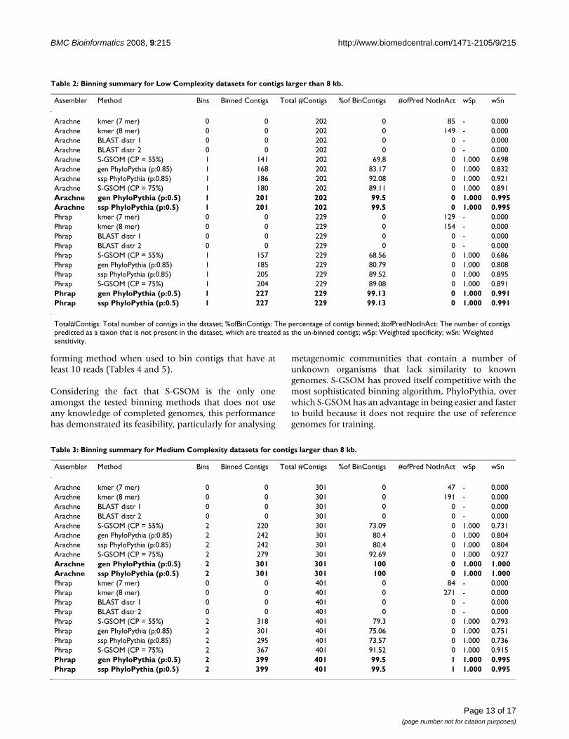
Two confidence settings of S-GSOM (high confidence –CP = 55% and low confidence – CP = 75%) were tested onthe simulated metagenomic data, which correspond totwo different settings of PhyloPythia. The S-GSOMs weretrained using parameters specified in Section 7 of the sup-plementary materials and the final feature maps are alsoprovided there. The binning results of S-GSOM, PhyloPy-thia, k-mer and BLAST on the simLC (Tables 2 and 4) andthe simMC (Tables 3 and 5) datasets are reported here. Atthe order level, the results for a different complexity data-set are shown in two separate tables, one for binning con-tigs greater and equal to 8 kb length and one for binningcontigs with at least 10 reads. Details of the datasets at dif-ferent taxonomic levels are also provided in Section 1 ofthe supplementary materials. Performance evaluationresults at class level and family level are included in Sec-tion 6 of the supplementary materials and all contigassignments can be downloaded from S-GSOMhomepage [50]. Note that the published results in Mavro-matis et al. used simple averages of all bins regardless oftheir sizes (number of contigs in a bin). Here we use aweighted average that gives higher weighting to larger binsto better reflect the amount of correctly binned contigs.The exact step of performance evaluation is provided inSection 5 of the supplementary materials.

The results in Table 2 and 3 showed that S-GSOM per-formed reasonably for binning contigs longer than 8 kb,where it is more accurate than all settings of k-mer andBLAST binning methods, but was outperformed by Phy-loPythia in both confidence settings (CP = 75% vs p = 0.5and CP = 55% vs p = 0.85) regardless of data complexityand the assembler used. Nevertheless, S-GSOM still per-formed better than PhyloPythia for the simMC, particu-larly in terms of sensitivity, i.e. having a higher truepositive rate, when the reference taxonomic level was atthe family level (see Section 6(ii) of the supplementarymaterials). While PhyloPythia performed best for all ≥ 8kb tests, the S-GSOM binning method was the best-per-



forming method when used to bin contigs that have atleast 10 reads (Tables 4 and 5).

Considering the fact that S-GSOM is the only oneamongst the tested binning methods that does not useany knowledge of completed genomes, this performancehas demonstrated its feasibility, particularly for analysing

metagenomic communities that contain a number ofunknown organisms that lack similarity to knowngenomes. S-GSOM has proved itself competitive with themost sophisticated binning algorithm, PhyloPythia, overwhich S-GSOM has an advantage in being easier and fasterto build because it does not require the use of referencegenomes for training.

Table 2: Binning summary for Low Complexity datasets for contigs larger than 8 kb.

Assembler Method Bins Binned Contigs Total #Contigs %of BinContigs #ofPred NotInAct wSp wSn

Arachne kmer (7 mer) 0 0 202 0 85 - 0.000Arachne kmer (8 mer) 0 0 202 0 149 - 0.000Arachne BLAST distr 1 0 0 202 0 0 - 0.000Arachne BLAST distr 2 0 0 202 0 0 - 0.000Arachne S-GSOM (CP = 55%) 1 141 202 69.8 0 1.000 0.698Arachne gen PhyloPythia (p:0.85) 1 168 202 83.17 0 1.000 0.832Arachne ssp PhyloPythia (p:0.85) 1 186 202 92.08 0 1.000 0.921Arachne S-GSOM (CP = 75%) 1 180 202 89.11 0 1.000 0.891Arachne gen PhyloPythia (p:0.5) 1 201 202 99.5 0 1.000 0.995Arachne ssp PhyloPythia (p:0.5) 1 201 202 99.5 0 1.000 0.995Phrap kmer (7 mer) 0 0 229 0 129 - 0.000Phrap kmer (8 mer) 0 0 229 0 154 - 0.000Phrap BLAST distr 1 0 0 229 0 0 - 0.000Phrap BLAST distr 2 0 0 229 0 0 - 0.000Phrap S-GSOM (CP = 55%) 1 157 229 68.56 0 1.000 0.686Phrap gen PhyloPythia (p:0.85) 1 185 229 80.79 0 1.000 0.808Phrap ssp PhyloPythia (p:0.85) 1 205 229 89.52 0 1.000 0.895Phrap S-GSOM (CP = 75%) 1 204 229 89.08 0 1.000 0.891Phrap gen PhyloPythia (p:0.5) 1 227 229 99.13 0 1.000 0.991Phrap ssp PhyloPythia (p:0.5) 1 227 229 99.13 0 1.000 0.991

Total#Contigs: Total number of contigs in the dataset; %ofBinContigs: The percentage of contigs binned; #ofPredNotInAct: The number of contigs predicted as a taxon that is not present in the dataset, which are treated as the un-binned contigs; wSp: Weighted specificity; wSn: Weighted sensitivity.

Table 3: Binning summary for Medium Complexity datasets for contigs larger than 8 kb.


Arachne kmer (7 mer) 0 0 301 0 47 - 0.000Arachne kmer (8 mer) 0 0 301 0 191 - 0.000Arachne BLAST distr 1 0 0 301 0 0 - 0.000Arachne BLAST distr 2 0 0 301 0 0 - 0.000Arachne S-GSOM (CP = 55%) 2 220 301 73.09 0 1.000 0.731Arachne gen PhyloPythia (p:0.85) 2 242 301 80.4 0 1.000 0.804Arachne ssp PhyloPythia (p:0.85) 2 242 301 80.4 0 1.000 0.804Arachne S-GSOM (CP = 75%) 2 279 301 92.69 0 1.000 0.927Arachne gen PhyloPythia (p:0.5) 2 301 301 100 0 1.000 1.000Arachne ssp PhyloPythia (p:0.5) 2 301 301 100 0 1.000 1.000Phrap kmer (7 mer) 0 0 401 0 84 - 0.000Phrap kmer (8 mer) 0 0 401 0 271 - 0.000Phrap BLAST distr 1 0 0 401 0 0 - 0.000Phrap BLAST distr 2 0 0 401 0 0 - 0.000Phrap S-GSOM (CP = 55%) 2 318 401 79.3 0 1.000 0.793Phrap gen PhyloPythia (p:0.85) 2 301 401 75.06 0 1.000 0.751Phrap ssp PhyloPythia (p:0.85) 2 295 401 73.57 0 1.000 0.736Phrap S-GSOM (CP = 75%) 2 367 401 91.52 0 1.000 0.915Phrap gen PhyloPythia (p:0.5) 2 399 401 99.5 1 1.000 0.995Phrap ssp PhyloPythia (p:0.5) 2 399 401 99.5 1 1.000 0.995



Discussion and conclusionRecently, the importance of environmental genomics hasbeen recognised [51,52] and more environmentalsequencing projects are being undertaken [1-3,18]. Mostof the current methods of binning compare a sequencefragment to a reference set of genomes. Such methodstend to have high assignment accuracy particularly whena strong similarity exists between the reference and envi-ronmental genomes, either at the compositional or

sequence level. However, the performance declines drasti-cally if the best match found is still quite different fromthe one being queried. On the contrary, extracting refer-ence sequences from within the metagenome, as in S-GSOM, will ensure better matching. It also facilitates ameans of exploring species that have not yet been identi-fied. In fact, such reference information from longerassembled contigs was used in the binning process of two

Table 4: Binning summary for Low Complexity datasets for contigs with at least 10 reads.


Arachne kmer (7 mer) 0 0 367 0 168 - 0.000Arachne kmer (8 mer) 0 0 367 0 312 - 0.000Arachne BLAST distr 1 0 0 367 0 0 - 0.000Arachne BLAST distr 2 0 0 367 0 0 - 0.000Arachne S-GSOM (CP = 55%) 3 295 367 80.38 0 1.000 0.798Arachne gen PhyloPythia (p:0.85) 2 214 367 58.31 0 1.000 0.583Arachne ssp PhyloPythia (p:0.85) 2 236 367 64.31 0 1.000 0.638Arachne S-GSOM (CP = 75%) 3 343 367 93.46 0 0.950 0.926Arachne gen PhyloPythia (p:0.5) 2 292 367 79.56 0 1.000 0.796Arachne ssp PhyloPythia (p:0.5) 2 296 367 80.65 0 1.000 0.798Phrap kmer (7 mer) 2 3 482 0.62 159 1.000 0.000Phrap kmer (8 mer) 3 17 482 3.53 281 1.000 0.000Phrap BLAST distr 1 0 0 482 0 0 - 0.000Phrap BLAST distr 2 0 0 482 0 1 - 0.000Phrap S-GSOM (CP = 55%) 8 381 482 79.05 9 1.000 0.728Phrap gen PhyloPythia (p:0.85) 3 236 482 48.96 0 1.000 0.488Phrap ssp PhyloPythia (p:0.85) 3 272 482 56.43 0 1.000 0.560Phrap S-GSOM (CP = 75%) 8 443 482 91.91 9 1.000 0.840Phrap gen PhyloPythia (p:0.5) 4 368 482 76.35 1 1.000 0.759Phrap ssp PhyloPythia (p:0.5) 5 387 482 80.29 1 1.000 0.797

Table 5: Binning summary for Medium Complexity datasets for contigs with at least 10 reads.


Arachne kmer (7 mer) 1 2 1372 0.15 133 1.000 0.000Arachne kmer (8 mer) 0 0 1372 0 1241 - 0.000Arachne BLAST distr 1 0 0 1372 0 0 - 0.000Arachne BLAST distr 2 0 0 1372 0 1 - 0.000Arachne S-GSOM (CP = 55%) 5 1061 1372 77.33 0 0.998 0.768Arachne gen PhyloPythia (p:0.85) 3 562 1372 40.96 0 1.000 0.409Arachne ssp PhyloPythia (p:0.85) 3 657 1372 47.89 0 1.000 0.478Arachne S-GSOM (CP = 75%) 5 1253 1372 91.33 0 0.983 0.897Arachne gen PhyloPythia (p:0.5) 4 1036 1372 75.51 6 1.000 0.753Arachne ssp PhyloPythia (p:0.5) 4 1102 1372 80.32 4 1.000 0.802Phrap kmer (7 mer) 1 1 1980 0.05 163 1.000 0.000Phrap kmer (8 mer) 2 391 1980 19.75 1457 1.000 0.000Phrap BLAST distr 1 0 0 1980 0 2 - 0.000Phrap BLAST distr 2 0 0 1980 0 3 - 0.000Phrap S-GSOM (CP = 55%) 8 1409 1980 71.16 9 0.995 0.686Phrap gen PhyloPythia (p:0.85) 3 799 1980 40.35 1 1.000 0.404Phrap ssp PhyloPythia (p:0.85) 3 844 1980 42.63 1 1.000 0.426Phrap S-GSOM (CP = 75%) 8 1708 1980 86.26 9 0.991 0.816Phrap gen PhyloPythia (p:0.5) 5 1484 1980 74.95 6 1.000 0.745Phrap ssp PhyloPythia (p:0.5) 5 1524 1980 76.97 4 1.000 0.767



prominent metagenomic projects for low-diversity micro-bial communities [1,4].

S-GSOM enables the clustering of sequence fragments,with phylogenetical meaning, by using very smallamounts of sequence fragments around the highly con-served genes as seeds. It has several advantages over otherunsupervised and semi-supervised clustering algorithms.First and most importantly, due to its visualisation prop-erty, S-GSOM allows the user to visually identify one ortwo relatively abundant species that do not have any seed,as demonstrated earlier, by using CP contour displaytogether with inter-node distances. However, to identifyunseeded clusters, it is necessary to have a larger numberof fragments in the unseeded cluster, at least as many asthe seeded clusters, i.e. the species is relatively abundant.If the unseeded clusters have far less samples than theseeded clusters, the unseeded cluster may be assigned tothe other clusters at low CP values, or be considered aspart of the border of neighbouring clusters and thusbecome hardly detectable. On the other hand, if theunseeded clusters have far more samples than the seededclusters, the clustering percentage needs to be set to alower value, as otherwise there will be more incorrectlyassigned samples.

The other advantages of S-GSOM include: 1) sequencescan easily be reassigned without retraining by varying theCP that is directly related to confident assignation, 2) theability to function as a fully automated clustering process,3) the potential use as a visualisation aid for identifyingunseeded clusters with iso-CP contours and inter-nodedistances, and 4) this technique can easily be applied toother applications when the labelled data is very limitedbut a lot of unlabelled data is available.

For the discovery of sequences of unknown microorgan-isms using S-GSOM, it should be expected that seeds mayor may not be available. When seeds are available, S-GSOM allows the identification of relationships betweenthe seed-associated clusters based on phylogenetic analy-sis of 16S rRNA sequences. If the phylogenetic analysisdetects any unknown microorganism, we will be able todiscover the sequences associated with this organism fromits 16S rRNA sequences using S-GSOM. This function willbe of great assistance in sorting sequences in metagen-omic datasets according to phylogenetic relationships.However, if no seed is available, it means that there is no16S rRNA sequence in the datasets for assessing the phyl-ogenetic relationships of this cluster. In such circum-stances, we can still obtain the sequences in the possiblebins, which were identified by using the iso-CP contourmap, then compare the sequences with existing databasesby BLAST searching. If any marker gene is detected, suchas elongation factors and/or cytochrome oxidase, then we

may assess whether these sequences are from unknown orknown microorganisms by phylogenetic analysis.

In the results section, we noted a major requirement forthe optimal performance of S-GSOM. As the proposedalgorithm uses seeds to assign more unknown fragments,poor seeds that are at the boundary of clusters, which areambiguous in themselves, can greatly affect the resultingassignment. This problem can possibly be solved byobserving the data distribution density around the seeds.For instance, if a seed occupies a single node and its sur-rounding nodes also contain fewer samples, the seed hasa high chance of being a poor seed. While a choice of CP= 55% yielded accurate sequence assignment in the twoseparate tests, a user can opt to use a lower clustering per-centage (e.g. CP = 35%) for more confident assignment atthe cost of fewer sequences being assigned. Conversely,using a higher CP value (e.g. CP = 75%) will assign morefragments but risk incorrect assignments. This feature isalso evident in the tests that use simulated metagenomicdata, where S-GSOM traded specificity for an increase insensitivity.

Although these composition-based binning methodshave shown good results, currently they are hindered bythe requirement of long sequence length. This limitationof length is partially due to the occurrence of chimericsequences from cloning procedures of experiments andfrom the incorrect assembly of sequences. The formersource of chimeric sequences can be reduced by improv-ing the sequence strategy, such as using a Roche 454genome sequencer FLX, which excludes sequence cloningand hence generates less chimeric sequences. The lattersource of chimeric sequences is caused by the incompati-ble design of the currently available assemblers. Theseassemblers are commonly designed to assemble all readsinto one single genome. However, this application doesnot satisfy the requirement of metagenomic datasetswhich are of poor coverage depth and contain multiplegenomes. As a result, it leads to the occurrence of chimericsequences when highly conserved stretches of sequences,e.g. transposases, are shared by multiple species or strains.Mavromatis et al. [7] tested the simulated metagenomicdatasets and showed that the numbers of chimericsequence became significant for the assembled shortsequences, e.g. < 8 kb, and led to the low quality of bin-ning. Therefore, if the number of chimeric sequences isreduced, the required sequence length can also bereduced. To help the reduction of chimeric sequences, wesuggest including the compositional information in theassembling level.

Authors' contributionsCKKC designed the overall study, implemented the algo-rithm and performed analysis. ALH contributed to the



design of the experiments and interpretation and analysisof results. SLT designed the algorithm with CKKC and bio-logical aspects of the study. All authors contributed to thepreparation of the manuscript, also read and approved thefinal manuscript.

Additional material

AcknowledgementsWe thank K. Mavromatis of DOE Joint Genome Institute for evaluating the results for S-GSOM on their simulated metagenome data and for discussing and clarifying their results.

References1. Tyson GW, Chapman J, Hugenholtz P, Allen EE, Ram RJ, Richardson

PM, Solovyev VV, Rubin EM, Rokhsar DS, Banfield JFB: Communitystructure and metabolism through reconstruction of micro-bial genomes from the environment. Nature 2004,428(6978):37-43.

2. Venter JC, Remington K, Heidelberg JF, Halpern AL, Rusch D, EisenJA, Wu D, Paulsen I, Nelson KE, Nelson W, Fouts DE, Levy S, KnapAH, Lomas MW, Nealson K, White O, Peterson J, Hoffman J, ParsonsR, Baden-Tillson H, Pfannkoch C, Rogers Y-H, Smith HOB: Environ-mental Genome Shotgun Sequencing of the Sargasso Sea.Science 2004, 304(5667):66-74.

3. Tringe SG, von Mering C, Kobayashi A, Salamov AA, Chen K, ChangHW, Podar M, Short JM, Mathur EJ, Detter JC, Bork P, Hugenholtz P,Rubin EMB: Comparative Metagenomics of Microbial Com-munities. Science 2005, 308(5721):554-557.

4. Woyke T, Teeling H, Ivanova NN, Huntemann M, Richter M, Gloeck-ner FO, Boffelli D, Anderson IJ, Barry KW, Shapiro HJ, Szeto E, Kyrpi-des NC, Mussmann M, Amann R, Bergin C, Ruehland C, Rubin EM,Dubilier N: Symbiosis insights through metagenomic analysisof a microbial consortium. Nature 2006, 443(7114):950-955.

5. Rusch DB, Halpern AL, Sutton G, Heidelberg KB, Williamson S,Yooseph S, Wu D, Eisen JA, Hoffman JM, Remington K, Beeson K,Tran B, Smith H, Baden-Tillson H, Stewart C, Thorpe J, Freeman J,Andrews-Pfannkoch C, Venter JE, Li K, Kravitz S, Heidelberg JF,Utterback T, Rogers Y-H, Falcón LI, Souza V, Bonilla-Rosso G,Eguiarte LE, Karl DM, Sathyendranath S, et al.: The Sorcerer II Glo-bal Ocean Sampling Expedition: Northwest Atlantic throughEastern Tropical Pacific. PLoS Biology 2007, 5(3):e77.

6. Yooseph S, Sutton G, Rusch DB, Halpern AL, Williamson SJ, Reming-ton K, Eisen JA, Heidelberg KB, Manning G, Li W, Jaroszewski L, Cie-plak P, Miller CS, Li H, Mashiyama ST, Joachimiak MP, van Belle C,Chandonia J-M, Soergel DA, Zhai Y, Natarajan K, Lee S, Raphael BJ,Bafna V, Friedman R, Brenner SE, Godzik A, Eisenberg D, Dixon JE,Taylor SS, et al.: The Sorcerer II Global Ocean Sampling Expe-dition: Expanding the Universe of Protein Families. PLoS Biol-ogy 2007, 5(3):e16.

7. Mavromatis K, Ivanova N, Barry K, Shapiro H, Goltsman E, McHardyAC, Rigoutsos I, Salamov A, Korzeniewski F, Land M, Lapidus A, Grig-oriev I, Richardson P, Hugenholtz P, Kyrpides NC: Use of simulateddata sets to evaluate the fidelity of metagenomic processingmethods. Nature Method 2007, 4(6):495-500.

8. Bentley SD, Parkhill J: Comparative genomic structure ofprokaryotes. Annual Review of Genetics 2004, 38:771-792.

9. Bailly-Bechet M, Danchin A, Iqbal M, Marsili M, Vergassola M: CodonUsage Domains over Bacterial Chromosomes. PLoS Computa-tional Biology 2006, 2(4):e37.

10. Karlin S, Mrazek J, AM C: Compositional biases of bacterialgenomes and evolutionary implications. Journal of Bacteriology1997, 179(12):3899-3913.

11. Sandberg R, Winberg G, Branden C-I, Kaske A, Ernberg I, Coster J:Capturing Whole-Genome Characteristics in ShortSequences Using a Naive Bayesian Classifier. Genome Res2001, 11(8):1404-1409.

12. Deschavanne P, Giron A, Vilain J, Fagot G, Fertil B: Genomic signa-ture: characterization and classification of species assessedby chaos game representation of sequences. Mol Biol Evol 1999,16(10):1391-1399.

13. Abe T, Kanaya S, Kinouchi M, Ichiba Y, Kozuki T, Ikemura TB: Infor-matics for Unveiling Hidden Genome Signatures. Genome Res2003, 13(4):693-702.

14. Abe T, Sugawara H, Kinouchi M, Kanaya S, Ikemura T: Novel Phyl-ogenetic Studies of Genomic Sequence Fragments Derivedfrom Uncultured Microbe Mixtures in Environmental andClinical Samples. DNA Res 2005, 12(5):281-290.

15. McHardy AC, Martin HG, Tsirigos A, Hugenholtz P, Rigoutsos I:Accurate phylogenetic classification of variable-length DNAfragments. Nature Methods 2007, 4(1):63-72.

16. Teeling H, Meyerdierks A, Bauer M, Amann R, Glockner FOB: Appli-cation of tetranucleotide frequencies for the assignment ofgenomic fragments. Environmental Microbiology 2004,6(9):938-947.

17. Teeling H, Waldmann J, Lombardot T, Bauer M, Glockner FB:TETRA: a web-service and a stand-alone program for theanalysis and comparison of tetranucleotide usage patterns inDNA sequences. BMC Bioinformatics 2004, 5(1):163.

18. Chen K, Pachter LB: Bioinformatics for Whole-Genome Shot-gun Sequencing of Microbial Communities. PLoS ComputationalBiology 2005, 1(2):e24.

19. Alahakoon LD, Halgamuge SK, Srinivasan B: Dynamic self-organiz-ing maps with controlled growth for knowledge discovery.IEEE Transactions on Neural Networks 2000, 11(3):601-614.

20. Blackmore J, Miikkulainen R: Visualizing High-DimensionalStructure with the Incremental Grid Growing Neural Net-work. Machine Learning: Proceedings of the 12th International Confer-ence 1995:55-63.

21. Alahakoon LD: Controlling the spread of dynamic self-organis-ing maps. Neural Computing & Applications 2004, 13(2):168-174.

22. Chan C-KK, Hsu AL, Tang S-L, Halgamuge SK: Using Growing Self-Organising Maps to Improve the Binning Process in Environ-mental Whole-Genome Shotgun Sequencing. Journal of Bio-medicine and Biotechnology 2008, 2008:Article ID 513701:10.doi:10.1155/2008/513701.

23. NCBI Database [http://www.ncbi.nlm.nih.gov]24. Kudo Y, Kanaya S: Consensus Genic Sequences in Bacterial

rRNA-tRNA Gene Clusters. In Proceedings of Genome InformaticsWorkshop 1995: Dec 11–12 1995; Pacific Convention Plaza, Yokohama,Japan Universal Academy Press, Tokyo; 1995.

25. RDP database [http://rdp.cme.msu.edu]26. Ward DM, Weller R, Bateson MM: 16S rRNA sequences reveal

numerous uncultured microorganisms in a natural commu-nity. Letters To Nature 1990, 345:63-65.

27. Thompson JR, Pacocha S, Pharino C, Klepac-Ceraj V, Hunt DE, BenoitJ, Sarma-Rupavtarm R, Distel DL, Polz MFB: Genotypic Diversity

Additional File 1Supplementary materials. This file is in pdf format. Section 1 provides details of all datasets used in this article. Section 2 gives descriptions of the semi-supervised algorithms, COP K-Means, Constrained K-Means, Seeded K-Means and Transductive SVM, used in the comparison with S-GSOM. Section 3 describes two popular clustering quality measures, the Adjusted Rand Index and Weighted F-Measure, in detail. Sections 4–7 provide more information on the experiments with simulated metagen-omic datasets. Section 4 briefly describes the three binning algorithms, BLAST, k-mer and PhyloPythia. Section 5 describes the steps used to eval-uate binning results of methods. Section 6 shows the detailed results of S-GSOM for all individual bins at different taxonomic levels for the simu-lated metagenomic dataset tests. Section 7 provides the training parame-ters used for S-GSOM and the resultant trained GSOM maps. Section 8 shows an example graph to demonstrate the relationship between CP value and the percentage of assigned samples. Finally, Section 9 lists the refer-ences used in the supplementary material.Click here for file[http://www.biomedcentral.com/content/supplementary/1471-2105-9-215-S1.pdf]


http://www.biomedcentral.com/content/supplementary/1471-2105-9-215-S1.pdf














































http://www.ncbi.nlm.nih.gov

http://rdp.cme.msu.edu






Publish with BioMed Central and every scientist can read your work free of charge

"BioMed Central will be the most significant development for disseminating the results of biomedical research in our lifetime."

Sir Paul Nurse, Cancer Research UK

Your research papers will be:

available free of charge to the entire biomedical community

peer reviewed and published immediately upon acceptance

cited in PubMed and archived on PubMed Central

yours — you keep the copyright

Submit your manuscript here:http://www.biomedcentral.com/info/publishing_adv.asp

BioMedcentral

Within a Natural Coastal Bacterioplankton Population. Sci-ence 2005, 307(5713):1311-1313.

28. Kohonen T: The self-organizing map. Proceedings of the IEEE1990, 78(9):1464-1480.

29. Kohonen T: Self-Organizing Maps. Volume 30. Third edition. Ber-lin, Heidelberg, New York: Springer; 2001.

30. Kohonen T: Analysis of processes and large data sets by a self-organizing method. Intelligent Processing and Manufacturing of Mate-rials 1999:27-36.

31. Hsu AL, Halgamuge SK: Enhancement of topology preservationand hierarchical dynamic self-organising maps for data visu-alisation. International Journal of Approximate Reasoning 2003, 32(2–3):259-279.

32. Hsu AL, Tang S-L, Halgamuge SK: An unsupervised hierarchicaldynamic self-organizing approach to cancer class discoveryand marker gene identification in microarray data. Bioinfor-matics 2003, 19(16):2131-2140.

33. Reinhard J, Chan C-KK, Halgamuge SK, Tang S-L, Kruse R: RegionIdentification on a Trained Growing Self-Organizing Map forSequence Separation between Different PhylogeneticGenomes. In BIOINFO 2005: 22–24 Sep 2005; Busan Korea: KAISTPRESS; 2005:124-129.

34. Hsu A, Halgamuge S: Semi-supervised learning of dynamic self-organising maps. Lecture Notes in Computer Science 2006,4232:915-924.

35. Adams R, Bischof L: Seeded region growing. Pattern Analysis andMachine Intelligence, IEEE Transactions on 1994, 16(6):641-647.

36. Herrmann L, Ultsch A: Label propagation for semi-supervisedlearning in self-organizing maps. In The 6th International Work-shop on Self-Organizing Maps (WSOM 2007): 3–6 Sep 2007; BielefeldGermany: Neuroinformatics Group; 2007.

37. Wagstaff K, Cardie C, Rogers S, Schroedl S: Constrained K-meansClustering with Background Knowledge. Proceedings of 18thInternational Conference on Machine Learning (ICML-01) 2001:577-584.

38. Basu S, Banerjee A, Mooney RJ: Semi-supervised Clustering bySeeding. Proceedings of the Nineteenth International Conference onMachine Learning (ICML-2002): July 2002; Sydney, Australia 2002:19-26.

39. Joachims T: Transductive inference for text classification usingsupport vector machines. In Proceedings of ICML-99, 16th Interna-tional Conference on Machine Learning Morgan Kaufmann Publishers,San Francisco, US; 1999:200-209.

40. Bruzzone L, Chi M, Marconcini M: A Novel Transductive SVM forSemisupervised Classification of Remote-Sensing Images.Geoscience and Remote Sensing, IEEE Transactions on 2006,44(11):3363-3373.

41. Hubert L: Comparing Partitions. Journal of Classification 1985,2:193-218.

42. van Rijsbergen CJ: Information Retrieval. 2nd edition. London:Butterworths; 1979.

43. SVMlight homepage [http://svmlight.joachims.org]44. FAMeS database [http://fames.jgi-psf.org]45. Batzoglou S, Butler J, Berger B, Gnerre S, Jaffe DB, Stanley K, Lander

ES, Mauceli E, Mesirov JP: ARACHNE: a whole-genome shotgunassembler. Genome Res 2002, 12(1):177-189.

46. Phrap Assembler [http://www.phrap.org]47. Aparicio S, Chia J-M, Hoon S, Putnam N, Christoffels A, Chapman J,

Stupka E, Dehal P, Rash S: Whole-genome shotgun assemblyand analysis of the genome of Fugu rubripes. Science 2002,297(Aug):1301-1310.

48. Strous M, Pelletier E, Mangenot S, Rattei T, Lehner A, Taylor M, HornM, Daims H, Bartol-Mavel D, Wincker P, Barbe V, Fonknechten N,Vallenet D, Segurens B, Schenowitz-Truong C, Médigue C, CollingroA, Snel B, Dutilh B, Op den Camp H, Drift C van der, Cirpus I, Pas-Schoonen K van de, Harhangi H, van Niftrik L, Schmid M, Keltjens J,Vossenberg J van de, Kartal B, Meier H, et al.: Deciphering the evo-lution and metabolism of an anammox bacterium from acommunity genome. Nature 2006, 440(7085):790-794.

49. Martin HG, Ivanova N, Kunin V, Warnecke F, Barry KW, McHardyAC, Yeates C, He S, Salamov AA, Szeto E, Dalin E, Putnam NH, Sha-piro HJ, Pangilinan JL, Rigoutsos I, Kyrpides NC, Blackall LL, McMahonKD, Hugenholtz P: Metagenomic analysis of two enhanced bio-logical phosphorus removal (EBPR) sludge communities.Nature Biotechnology 2006, 24(10):1263-1269.

50. S-GSOM homepage [http://www.mame.mu.oz.au/~ckkc/S-GSOM]

51. Foerstner KU, Mering Cv, Bork P: Comparative analysis of envi-ronmental sequences: potential and challenges. PhilosophicalTransactions of the Royal Society B: Biological Sciences 2006,361(1467):519-523.

52. Deutschbauer AM, Chivian D, Arkin AP: Genomics for environ-mental microbiology. Current Opinion in Biotechnology – Environ-mental biotechnology/Energy biotechnology 2006, 17(3):229-235.






http://svmlight.joachims.org

http://fames.jgi-psf.org



http://www.phrap.org








http://www.mame.mu.oz.au/~ckkc/S-GSOM

http://www.mame.mu.oz.au/~ckkc/S-GSOM


http://www.biomedcentral.com/info/publishing_adv.asp


Binning sequences using very sparse labels within a metagenome

Documents

Transcript of Binning sequences using very sparse labels within a metagenome