IEEE/ASME TRANSACTIONS ON MECHATRONICS, VOL. 15, NO. 4, AUGUST 2010 527

Performance Analysis of the CCD Pixel BinningOption in Particle-Image Velocimetry Measurements

Humbat Nasibov, Alisher Kholmatov, Basak Akselli, Adalat Nasibov, and Sakir Baytaroglu

Abstract—This paper proposes convenient methods to increasethe dynamic speed range in particle-image velocimetry (PIV) mea-surements, which employ a charge-coupled device (CCD) camerabinning option. Although the binning procedure decreases spatialresolution along specified dimensions, its ability to increase thecamera frame rate and preserve the field-of-view are importantadvantages, which need to be thoroughly investigated. In orderto demonstrate the advantages of the CCD binning option, wehave carried out experiments both on static images of in-planeparticle displacements and on dynamic images of real-fluid flows.In the first experiment, we have analyzed static images of 0.5, 1,and 1.9 µm size fluorescent polystyrene microparticles placed onthick quartz glass plate and illuminated by high-power LED. Thein-plane images were captured at various CCD binning options,the distance between particles was then calculated using cross-correlation analysis and a subpixel interpolation scheme based ona Gaussian filter. In the second experiment, the fluid flow in a 30 ×300 × 50 000 µm microchannel was recorded at various CCDbinning modes, and then, evaluated using ensemble-averaged nor-malized cross-correlation analysis with Gaussian subpixel interpo-lation. Velocity profiles obtained at various CCD binning modeswere compared with those obtained at the normal mode. Erroranalysis has shown that despite the loss of the spatial resolution,the advantages of pixel binning, specifically increased sensitivityand a total full-frame rate, can be useful in PIV measurements,especially in laminar-fluid flows.

Index Terms—Binning, charge-coupled device (CCD), correla-tion, fluid flow measurement, particle-image velocimetry (PIV),particle tracking.

I. INTRODUCTION

DUE TO THE noncontact and nondestructive nature of mea-surements conducted in optical imaging metrology, the

field continues to draw interest from various fields of science andindustry. The role of the optical imaging metrology grows every-day, especially in performing various quantitative and qualitativeanalyses and for measurements of moving objects and mediumsdown to the micrometer size scale. Generally, the progress inthis field runs parallel with developments and improvements in

Manuscript received March 9, 2010; accepted May 12, 2010. Date of publi-cation June 28, 2010; date of current version July 28, 2010. Recommended byGuest Editor T. Fukuda.

H. Nasibov, A. Kholmatov, and A. Nasibov are with the National ResearchInstitute of Electronics and Cryptology, Scientific and Technical Research Coun-cil of Turkey, Gebze 41470, Turkey (e-mail: humbat@uekae.tubitak.gov.tr;alisher@uekae.tubitak.gov.tr; adalat@uekae.tubitak.gov.tr).

B. Akselli and S. Baytaroglu are with the National Metrology Institute, Scien-tific and Technical Research Council of Turkey, Gebze 41470, Turkey (e-mail:basak.akselli@ume.tubitak.gov.tr; sakir.baytaroglu@ume.tubitak.gov.tr).

Color versions of one or more of the figures in this paper are available onlineat http://ieeexplore.ieee.org.

Digital Object Identifier 10.1109/TMECH.2010.2051678

both visualization methods and digital image sensor technology.With the advent of epifluorescent microscopy and digital cam-eras, a variety of visualization methods have been developed.For example, in recent years, significant progress has been madein the applications of optical imaging methods in fluid and gasflow visualization [1]. One of the major logical extensions offlow visualization is the particle-image velocimetry (PIV). PIVis a noninvasive, full-field optical measuring technique, whichhas become the dominant tool for obtaining velocity informationin fluid motion [2]–[7]. In PIV experiments, the fluid of interestis seeded with fluorescent dyed micrometer or submicrometerscale sized free-floating probe particles. The full field-of-view(FOV) of epifluorescent imaging optics is used to observe a partof the channel illuminated by a sheet of bright light (high-powerpulse lasers with a wavelength corresponding to the fluorescenceexcitation of tracer particles). The position of these particles ata minimum of two instances of time is recorded by employinga high-speed camera. Then, by measuring the particle displace-ments, the motion of the fluid can be ascertained. Generally, PIVrequires the accurate, quantitative measurement of fluid velocityvectors at a large number of points simultaneously.

The other approach, particle-tracking velocimetry (PTV) dif-fers from PIV by the image processing methods used for extract-ing the underlying velocity fields. While PIV methods operateon gray-level images, utilizing cross correlation between in-terrogation volumes; in PTV, individual particles are identifiedand tracked from image to image. Generally, PTV methods areeither based on the nearest neighbor search with geometricalconstraints (using four or more consecutive frames) [8], or onbinary-image cross correlation (two frames) [9], which com-putes the cross correlation between regions around particles inthe first and the second frame [10]. To allow the unambiguous lo-cation of nearest neighbors, PTV required low-density particleimages. However, the introduction of “superresolution” algo-rithms [11] has allowed the extension of PTV to higher imagedensities. “Superresolution” algorithms use cross correlation toobtain a PIV vector field, and then, use this field to guide thesearch for particle matches in a subsequent PTV step [12].

Micron-resolution PIV (micro-PIV) [13]–[15] is a modifica-tion of PIV in order to access the small scales of microfluidicdevices. In a typical PIV experiment, a light sheet formed by alaser is used to illuminate only a section of the flow, where thethickness of the light sheet is smaller than the depth of focusof the image recording system. In most cases, this approachis impractical for micro-PIV, and instead so-called volume il-lumination is applied. Here, the whole volume of the flow isilluminated, where the FOV and depth of focus of the micro-scope objective defines the measurement volume.

1083-4435/$26.00 © 2010 IEEE

528 IEEE/ASME TRANSACTIONS ON MECHATRONICS, VOL. 15, NO. 4, AUGUST 2010

Nowadays, industrial and research applications of PIV/PTV/micro-PIV have extended from measuring the velocity of sandand dusts in tunnels to micro/nanofluid flows in microscale lab-on-a-chip devices. Various modifications of PIV are widely usedfor detection and control of chemical reactions, sample prepa-ration, variety of flow investigations, characterization of pres-sure and chemical sensors, microscale systems for biologicaldiagnostics, such as DNA analysis by means of polymerasechain reaction (PCR), pumping systems, miniaturized underwa-ter propulsion systems, etc. [16], [17].

Generally, PIV systems were designed by laboratory re-searchers for a better understanding of flow physics. In mostPIV experimental setups, illumination is provided using dualcavity lasers, whose output reaches several millijoule at pulselengths in the range of tens of nanoseconds. These systems arevery expensive and bulky. Currently, there is a trend toward de-signing cost-effective and transportable PIV systems. In [18],the possibility and versatility of using LED in micro-PIV se-tups for illumination was investigated. In [19], a cost-effectiveand miniature PIV system with LED illumination, which can beused as an industrial velocity sensor, is reported.

The maximum assessable velocity measurement of a flow isbounded by the frame rate (also referred as the speed) of theparticular camera being used. Obviously, the higher the framerate a camera can achieve, the more it costs; the cost growssignificantly with respect to the frame rate. In this paper, we in-vestigated the possibility of increasing the performance of LEDilluminated PIV systems by means of charge-coupled device(CCD) camera binning, which increases the frame rate (i.e.,dynamic velocity range) at the bearable cost of losing spatialresolution.

A. Digital PIV

The main issue in PIV experiments is the derivation of localdisplacement vectors from a sequence of particle-seeded flowimages, each with a known temporal separation.

There are two common methods of displacement recordingin PIV experiments.

1) Single frame/multiexposure, when two or more exposuresof the tracer particles are made on a single frame,

2) Multiframe/single exposure, when two or more exposuresof the particles are made, each on a separate frame.

The first method was widely used in early PIV measurements,when the tracer particle images were recorded by wet-film pho-tography. Due to the long winding time of the film betweenexposures, single frame/multiexposure was the most commonlypreferred recording method. The process of preparing and an-alyzing the negatives, printing and digitizing images, and per-forming displacements estimation required several hours of hardwork. Taking into account that a single-PIV experiment may in-volve hundreds of images, the complete process was very timeconsuming.

The second method became popular with the advent of digitalimaging technologies, which made PIV one of the fastest andmost accurate techniques for fluid flow velocity measurements.Digital cameras and computer systems make it possible to obtain

digitized images of separate frames for each exposure during ashort time and to transfer the digitized signal immediately to acomputer for automated analysis.

In order to carry out the calculation of a flow field, at least twoconsecutive frames, each containing corresponding displacedtracer particles (i.e., there must be some overlap between twoframes), must be captured. Then, these corresponding frames areparceled into interrogation spots, where within each spot overallparticle-displacement vectors are calculated using particle track-ing or correlation-based methods [20]. While there are a numberof factors affecting the accuracy and calculation capability of aPIV system, in the context of this study, we consider only the dy-namic velocity range and dynamic spatial range characteristicsas these are directly related to a capturing device used [21].

The dynamic velocity range is equal to the ratio betweenthe maximum and minimum assessable velocity measurementsa PIV system can attain under fixed instrumental parameters.This metric defines the upper limit on the resolvable velocityvariation within the flow. For instance, the system will be un-able to fully ascertain flow field if the dynamic velocity rangeis less than the magnitude of the velocity variation within theflow. The analogy can be made to the dynamic range of imagingand display devices, where when capturing a scene containinga dynamic range that exceeds that of the camera, there will bea loss of details on either low-light areas or high-light areas, orboth. High-dynamic velocity range is essential for characteri-zation of turbulent flows, where the velocity drastically variesacross the FOV. Contemporary PIV systems achieve dynamicvelocity ranges of an order of several hundred, but still this doesnot suffice for certain types of flows.

Similarly, the dynamic spatial range is defined by the ratio ofthe FOV in the object space to the smallest resolvable spatialvariation. This range corresponds to the number of nonoverlap-ping displacement vector measurements that can be done acrossthe FOV. Higher dynamic spatial range implies better capabilityto assess small-scale variation within the large-scale fluid mo-tion. Similarly, the analogy can be made to the spatial resolutionof imaging devices, where higher resolution implies acquisitionof finer details in the captured scene.

In the next section, we will investigate the CCD binningoption, which increases the dynamic velocity range of the PIVsystem at the expense of the dynamic spatial range, and analyzeits performance in PIV experiments.

B. CCD Binning

The heart of a digital imaging camera is a solid-state arraydetector (electronic imaging sensor), generally named CCD,which acts as a transducer of emanating light to a measurableelectrical signal. The CCD’s output signal represents the spa-tial distribution of light intensity (formed by means of imagingoptics) falling onto the imaging sensor.

An electronic imaging sensor is comprised of photon-sensitive regions called pixels. Each pixel converts photons intoelectrons according to its spectral sensitivity and incident lightintensity, accumulates electrons according to its well capac-ity during the exposure time (charge collection), and transfers

NASIBOV et al.: PERFORMANCE ANALYSIS OF THE CCD PIXEL BINNING OPTION IN PARTICLE-IMAGE VELOCIMETRY MEASUREMENTS 529

electrons via a charge-to-voltage converter according to its bitdepth and readout mechanism. Each of these processes, chargegeneration, collection, and transfer is accompanied with varioustypes of noise, which affects the quality of output image. Forinstance, a dark current noise is caused by thermal effects duringthe exposure time and generates nonphotonic charges in wells.The readout noise is added to total charges at all instants, whiletransferring charge from pixel to the on-chip amplifier, wherecharge is converted into an analog voltage.

Depending on a readout mechanism, there are two commontypes of CCD devices: full-frame transfer and interline trans-fer. Full-frame devices contain two identical arrays, namely, thephotosensitive and storage, where the later is shielded from light.The photosensitive array, during exposure time collects charge,and then, quickly transfers them to the storage area. While trans-ferring charges from the photoactive array to the storage array,an electromechanical shutter closes the photosensitive area andblocks the light. After completing the charge transfer, an elec-tromechanical shutter opens and the photosensitive array beginsexposing new image, while simultaneously the previous imageis being moved from the storage array to the charge-to-voltageconverter and output amplifier.

In the interline transfer CCD, a light-shielded storage area(vertical lines) is located within the active area of the CCD, be-tween columns of photoactive pixels. In these sensors, the read-out process is performed in two steps: the first being the parallelreadout step, which takes place at the end of exposure time. Thecharge from every pixel is simultaneously shifted directly totheir corresponding wells in the storage section (charge transferchannel). In the second, serial readout step, charge from the stor-age section is shifted row-by-row to output, charge-to-voltageconverter, and amplifier units. Detailed information about thesetwo CCD readout techniques and the working principles of CCDcan be found in [17] and [18].

In our paper, we will refer to the interline frame transfer CCD.The sum of exposure and readout times (including various inter-nal clocking pulse times) define the full-frame rate of a certaincamera in the given imaging conditions. Generally, the timeconsumed by the parallel readout is less than a millisecond andis negligible compared to the time required for serial readout,which depends on the CCD pixel resolution, more precisely,on the number of rows in the sensor array. Reduction of rownumber in the sensor array leads to a decrease in the readouttime, i.e., it increases the frame rate of the CCD, and however,this will also decrease the spatial resolution.

In recent years, CCD manufacturers have been supplyingtheir devices with very versatile options, such as the abilityto manipulate the CCD readout pattern, adjustable selectionof a region of interest (ROI), and flexible binning options.In ROI mode, often referred as “subwindowing,” it is pos-sible to select a specific portion (commonly rectangular) ofthe image by reading charges just from corresponding pixels.Since the number of pixels decreases, the frame rate increases.However, this mode reduces the FOV of the imaging system,whereas in PIV measurements, the tradeoff between reducedFOV and increased frame rate must be balanced. On the con-trary to ROI, the binning option, which is the other mode of han-

Fig. 1. Schematic representation of n × m binning mode.

dling the CCD output pattern, preserves the FOV of the camerasystem.

Binning is the process of combining multiple pixel chargesin horizontal, vertical, or in both directions into a single largercharge called “binned pixel” or “super pixel.” The binning pro-cess is performed after exposure time by a specialized controlof the serial and parallel registers in a CCD chip, prior to dig-itization in the on-chip circuitry. The charge of “super pixel”represents the sum of charges of all individual pixels beingbinned together. The CCD binning process affects spatial reso-lution, sensitivity, SNR, and frame rate of the imaging sensor.Let n and m be the numbers of pixels forming a super pixel invertical and horizontal directions, respectively. The value, in-crement, and relation between binning orders (i.e., n and m),depends on the particular sensor type. There are three types ofbinning mode: 1) n = m >1—“quadratic binning;” 2) n > m andn > 1—“vertical binning;” and 3) n < m and m >1—“horizontalbinning.”

In n × m binning mode, each super pixel represents the rect-angular area with n vertical and m horizontal pixels, as depictedin Fig. 1. Accordingly, the spatial resolution of the whole sen-sor (i.e., of the output image) diminishes by n times in verticaland by m times in horizontal directions. Any binning modepreserves the full FOV of the imaging optics. In the case ofquadratic binning n = m > 1, the spatial resolution of the im-age decreased n times in both directions and the dimensions ofthe output image is reduced by n2 times, keeping the inherentscale of the image. Any asymmetrical binning mode n �= m,n ≥ 1, and m ≥ 1 introduces scale distortion into the outputimage.

The electrons created by light during the exposure time arecollected in wells. The full-well capacity (evaluated in units ofnumbers of electrons) defines the maximum number of electronsthat a pixel can hold, and plays a dominant role in characteriz-ing the CCD’s dynamic range. If during the exposure time thenumber of photogenerated charges exceeds full-well capacity ofa pixel, charges will flow to the neighbor cells, if these wells aresaturated the charges will flow to the next adjacent pixels, etc.

This process is called “smearing” or “blooming,” whichcauses fully saturated streaks on the image destroying pixel in-formation. For most CCD, (except some special scientific CCD,where the capacity of storage wells is greater than the pixelwells, for on-chip averaging), the full-well capacity of activepixels and maximum charge transfer capacity of correspondingstorage registers are the same. Since the pixel well capacityis a physical property of the sensor, the binning process doesnot affect the well capacity. Therefore, at any binned mode, the

530 IEEE/ASME TRANSACTIONS ON MECHATRONICS, VOL. 15, NO. 4, AUGUST 2010

full-well capacity of “the super pixel” will be the same and equalto the full-well capacity of the single pixel.

However, in the binning mode due to the expansion of thephotosensitive area by n × m times, the sensitivity of the “su-per pixel” to the light increases. Accordingly, the number ofphotogenerated charges (over the super pixel) within a certaintime increases and the well filling process is faster. So, in orderto avoid saturation (blooming) effects, it is necessary to decrease(by n × m times) the exposure time.

The binning process positively influences SNR, such that itreduces the noise and improves the signal. Without the lossof generality, we separate noise sources into two groups: in-tegration time dependent noises (dark-current shot noise, pho-ton shot noise, photoresponse nonuniformity, and offset fixed-pattern noise) and readout noise (supporting integrated circuitthermal noise, reset noise, preamplifier, and converter noises).Each of the pixels forming the “super pixel” will contribute theirsignal and noise to the signal and noise of the “super pixel” in-dependently. According to the “propagation of uncertainties”calculation, which assumes that the noise inherent in a pixel isindependent of the noise present in any other pixel, for a set ofn × m pixels, where each constituent pixel has the same chargeand noise levels, the overall amount of the noise in the “superpixel” will be

√n × m times larger than the noise of each con-

stituent pixel. However, since exposure time must be decreasedby n × m times due to the averaging mechanism the overallnoise in the super pixels will be decreased to

√n × m/n × m,

i.e., 1/√

n × m.Readout noise is a fundamental trait of CCD’s, which is a

combination of the system noise components inherent to theoverall process—from charge transferring to converting theminto a voltage signal. The significant contribution to readoutnoise usually originates from the on-chip preamplifier, whichultimately limits a camera’s SNR. As readout noise is addeduniformly to every pixel value of the output image, reducing(by binning) pixel numbers n × m time will reduce readoutnoise contribution in the output image by n × m times. Theother primary feature of the binning option is a decreasing ofthe readout time, which leads to increase of the frame rate ofthe imaging sensor. This property is one of the most valuablebenefits of the binning option, which can be utilized in PIVmeasurements. The increase of the frame rate depends on theparticular binning type, which will be described in the follow-ing. For the sake of brevity, we will describe and analyze onlythe two-by-two (2 × 2, 2 × 1, 1 × 2) binning modes, whilethe higher order n × m binning modes (allowable by specifica-tion of certain CCD architecture numbers of n and m) can beinterpreted in the same way.

Fig. 2(a) shows a schematic representation (a part of the arraywith a 4 × 4 spatial resolution) of normal CCD pixel arrange-ment. Fig. 2(b) shows an image of four fluorescent particles,located on a glass plate and illuminated by two LEDs (the firstone for fluorescence excitation and the second, in peak wave-length at 800 nm, just in this case, for illumination of the wholescene) captured in normal mode of CCD (single-pixel readout).

Fig. 3(a) shows an example of quadratic 2 × 2 binning mech-anism, where “super pixel P’1” is formed by combining charges

Fig. 2. (a) Schematic representation of normal CCD pixel arrangement and(b) corresponding output image.

Fig. 3. (a) Schematic representation of quadratic—2 × 2 CCD pixel binningarrangement and (b) corresponding output image.

from four P1, P2, P5, P6 neighbor pixels, etc. Fig. 3(b) showsthe 2 × 2 binned image of the particles from Fig. 2(b). In com-parison with the single-pixel mode, in 2 × 2 binning mode, theparticle size on the image decreased two times in both direc-tions. In this mode, the spatial resolution of the image decreasesfour times. We will not discuss effects related to the fill fac-tor (the ratio of photosensitive area to the full area of imagingsensor), as most CCDs (including those utilized in this paper)are supplied with microlenses in front of active pixels, and willassume that the fill factor is about 100%.

Fig. 4(a) depicts the horizontal 1 × 2 binning mode, wherethe image spatial resolution in horizontal direction decreasestwo times. In this mode, the number of columns is halved,while keeping the number of rows is unchanged. As mentionedearlier, in interline CCD, the readout time is determined by thenumber of rows, so vertical binning does not affect the framerate. Fig. 4(b) shows the 1 × 2 binned image of the particlesfrom Fig. 2(b).

Fig. 5(a) depicts the vertical 2 × 1 binning mode, wherethe image spatial resolution in vertical direction decreases twotimes. Fig. 5(b) shows the 2 × 1 binned image of the parti-cles from Fig. 2(b). In vertical binning mode, the number ofthe columns remains unchanged, while the number of the rowsdecreases two times, which leads to a decrease in readout time,and increase in the frame rate. On the whole, the followingproperties of the vertical binning mode: improved SNR, pre-served FOV, and an unchanged remaining spatial resolution in

NASIBOV et al.: PERFORMANCE ANALYSIS OF THE CCD PIXEL BINNING OPTION IN PARTICLE-IMAGE VELOCIMETRY MEASUREMENTS 531

Fig. 4. (a) Schematic representation of horizontal—1×2 CCD pixel binningarrangement and (b) corresponding output image.

Fig. 5. (a) Schematic representation of vertical—2 × 1 CCD pixel binningarrangement and (b) corresponding output image.

horizontal direction, and an increased frame rate can be usedfor improvement of PIV measurement systems, especially, inmeasurements of laminar flows.

In the next sections, we will analyze the application of CCDbinning in PIV experiments.

II. EXPERIMENTAL SETUP

In this paper, we have performed two different experiments toanalyze the influence of the CCD binning options on PIV/PTVresults. The first experiment was aimed at assessing the effectsof particle-image deformation solely caused by the CCD bin-ning option. For this reason, displacement calculations wereperformed using only static images, which largely avoids allother errors inherently caused by the PIV method. In the secondexperiment, real-laminar flows were analyzed at each binningmode and compared to the results obtained in the normal mode.

A. Static-Image Experimental Setup

Fig. 6 shows a schematic representation of the experimentalsetup, where static images of particle in-plane displacements

Fig. 6. Schematic representation of the experimental setup.

were obtained using the inset denoted as (a). In this experi-ment, we fixed a glass plate with seeded particles onto a 2-D,computer-controlled linear translation stage. The samples wereprepared by laying an aqueous solution of 0.5, 1, and 1.9 µmsize green fluorescent polystyrene microspheres onto a high-quality quartz glass plates (thickness 0.8 mm). The glass plateswere then placed into a furnace in order to evaporate the watermolecules. The samples obtained were analyzed under micro-scope and the plate exhibiting the most homogenous distributionof particles was selected and used in the experiments. The FOVof the microscope was illuminated using a backlit illuminationconfiguration. The LED illumination (Lumileds, Luxeon) with470 nm peak wavelengths was focused on the backside of theglass plate. Imaging was realized by utilizing a Hirox variablezoom lens (1–10×) conjugated with a OL-700II objective. Inorder to image only the fluorescence excitation of particles andeliminate the LED illumination, a long pass filter was placed be-tween the objective and the CCD camera. Images were recordedwith a monochrome digital camera (Pixelfly) with an imageresolution of 1392 × 1024, a pixel size of 4.65 × 4.65 µm,and a full-resolution frame rate of 12 f/s. The camera supportsquadratic—2 × 2, horizontal—1 × 2, and vertical—2 × 1 bin-ning modes. In quadratic and vertical binning modes, the framerate of the camera increased up to 23 f/s, and in the verticalmode, the frame rate remained unchanged. In the experiments,the images were captured with full resolution (normal mode),and the 2 × 2, 1 × 2, and 2 × 1 binning modes. The soft-ware performed random movements of the glass plate in twodirections. Maximum displacement did not exceed 50% of themicroscope FOV. For every position, images were captured atnormal (full frame) and 2 × 2, 2 × 1, 1 × 2 binning modes.For each particle size, more then 100 frames were captured andused for distance calculations.

B. Real-Flow Experimental Setup

Dynamic flow experiments were conducted using the samesetup (see Fig. 6) with the only difference being that, in thiscase, the inset (b) was utilized. A programmable syringe pump

532 IEEE/ASME TRANSACTIONS ON MECHATRONICS, VOL. 15, NO. 4, AUGUST 2010

(NE-1000, New Era Pump Systems, Inc.) was used to pump thefluid through the microchannel. In the experiments, double dis-tilled water was seeded with spherical polystyrene fluorescentparticles (Duke Scientific, Palo Alto, CA). The density of par-ticles is approximately ρp = 1.05 g/cm3 , so they are expectedto be able to tag the flow streamlines without excessive slip.Real-flow measurements were performed using 1-µm-diameterparticles. According to the manufacturer certificate, the particle-size distribution’s standard deviation is about 0.011 µm. In theexperiments, the volumetric particle concentration was about0.2%.

We investigated steady-state laminar flows in 30 × 300 ×50000 µm microchannels. The microchannel holder wasmounted onto the precise alignment stage in a way that madeit possible adjusting the microscope focus onto different depthlevels inside the channel. The flow of particles was recorded at adepth of ∼15 µm. The flow velocity was regulated by adjustingthe pump’s output rate to the desired value.

We performed flow recording about 10 min after startingthe pump, so the flow measured inside the microchannel canbe considered as a pressure-driven steady-state uncompressedflow. The measurements were performed at three different bin-ning modes: with full resolution (single-pixel mode), the 2 × 2binning mode, and the 2 × 1 vertical binning mode. The home-made image recording software was able to record a cycle of PIVimages in the following way: it set the camera to the normal (nobinning) mode and captured 300 consecutive full-frame PIV im-age frames onto the computer RAM, then immediately switchedthe camera to the desired binning mode and captured 300 framesof binned image (see Section IV, Fig. 14). Just after finishing thiscycle, the captured frames were stored in an uncompressed TIFFformat to the hard disc storage, thereby avoiding any delay re-sulting from computer systems. Image analysis was carried outusing an in-house software written in MATLAB. Measurementswere carried out at room temperature, i.e., 23.0 ± 0.5 ◦C.

III. SUBPIXEL INTERPOLATION

Due to the discrete nature of digital imaging sensors, the directapplication of normalized cross-correlation procedure for thedisplacement estimation returns integer-based results. In otherwords, an error of ±0.5 pixels is present in the location of thecorrelation peak. In order to increase the accuracy of distanceestimation in PIV (i.e., to locate the correlation peak withinsubpixel accuracy), a variety of subpixel interpolation methods,such as parabolic curve fitting, center-of-mass, and Gaussiancurve fitting have been proposed [23]–[26]. In [27], a subpixelinterpolation method, which accounts for nonaxially orientated,elliptically shaped particle images, or correlation peaks is pro-posed. In this section, we first analyze the particle-image shapedistortions in each of the proposed binning mode, and then,derive the corresponding subpixel interpolation equations.

A. Study of Particle-Image Distorsions Introduced by theBinning Option by Means of the Autocorrelation Method

In PIV/PTV experiments, the exact center positions of theidentified particles at known instants of time are more important

than having a good picture ’’portrait” of the seeding particles.Any distortion caused by the image acquisition step, which doesnot affect the particle location information, can be eluded by de-termining the nature of this distortion and applying appropriatecorrections. In this section, we will analyze the shape distortionintroduced by the binning mode to the “portrait” of particles byemploying the autocorrelation function (ACF) [28], which canbe represented in a discrete form as follows [29]:

ACF(u, v) =[

1MN

] M −1∑u=0

N −1∑v=0

I(x, y)I(x + u, y + v) (1)

where M and N are the width and height of the image, I(x, y) isthe gray level of intensity at the (x, y) point, and u and v are theindependent parameters of summation. In this interpretation, theACF is considered as a two-point statistics method, which canbe viewed as a result of self cross-matching examination of theimage that quantifies the relationship between different pixels onthe image. Although the ACF and input image are 2-D functionsand their dimensions are exactly the same, this self-crossingprocess sums all point–point similarities of the image separatedwith a distance

√u2 + v2 , u ∈ [0,M − 1] and v ∈ [0, N − 1].

As a result, this summing process accumulates and reorganizesintrinsic similarities hidden in a given image. In our particularcase, when the image of only one particle is considered, ACFallows to determine shape and dimensions of the particle (inpixels). Among the major advantages of using a spatial ACF areits unbiased character (because no segmentation of the imageprior to analysis is necessary) and its capability to suppress thenoise [30]. ACF takes its maximum value at zero shifts (u = v =0), which represents the covariance of the image, which reflectsthe excitation intensity of the particle under consideration, aswell as the shot noise of the imaging system. Therefore, bycalculating the ACF of the particle image, we can estimate theshape and area of the particle fluorescence excitation even withthe presence of background noise.

For small shifts of u and v, the ACF values descend accord-ing to the expectation of finding pixels with either the same orneighboring gray-level intensity separated by the distance u orv. As for small shifts of u and v, the ACF renders the similar-ities of the optical density in the vicinity of individual pictureelements, which is a useful measure for shape description of theparticles. Besides the particle characteristics, the ACF peak con-tains the transfer functions of the imaging system. So, in equalimaging conditions (equal defocus and illumination), ACF canprovide information about image distortions, caused by the bin-ning option. We have captured fluorescent particle images atdifferent CCD binning modes, and then, analyzed their ACFresults. Fig. 7 shows the ACF of the same single-particle im-age, captured at: (a) normal mode, (b) –2 × 1, (c) –1 × 2, and(d) –2 × 2 binning modes. The analysis of the 2-D cross sec-tion at full-width at half-maximum (FWHM) of obtained 3-DACF surfaces shows that: 1) in the normal capturing mode, theshape of single particle is a circle with the radius R; 2) in 1 ×2 binning mode, the shape is transformed into vertical ellipsewith θ = π/2, and σx/σy = 0.5; 3) in 2 × 1 binning mode,the shape is transformed into horizontal ellipse with θ = 0, and

NASIBOV et al.: PERFORMANCE ANALYSIS OF THE CCD PIXEL BINNING OPTION IN PARTICLE-IMAGE VELOCIMETRY MEASUREMENTS 533

Fig. 7. Single-particle image and its ACF at different binning modes,(a) Without binning. (b) 2 × 1 vertical binning. (c) 1 × 2 horizontal binning.(d) 2 × 2 binning. (Images are scaled with preserving aspect ratio).

σx/σy = 2; and 4) in 2 × 2 binning mode, the shape is remainsthe circle with σx = σy = R/2, where θ is the angle between Xcoordinate line (in our case, motion direction) and major semi-axis, and σx, σy are the major and minor semiaxes of ellipse,respectively.

B. Subpixel Interpolation for Circular Image Case

In this paper, we have used 2-D Gaussian interpolation [2]in the cases of normal and 2 × 2 binning image acquisition

modes, as it best fits to the circular image shapes obtained by thecorresponding modes. Fig. 7(a) and (d) depict particle imagesobtained in the normal and 2 × 2 binning modes, respectively.In order to estimate subpixel displacement, a Gaussian surfaceis fitted to the local neighborhood around the peak of the cor-relation function. The maximum of the interpolated Gaussiansurface is located at ∆x, ∆y with respect to the index x0 , y0of the correlation peak. Assuming the correlation peak has aGaussian-distribution shape, the accurate location of the corre-lation peak is as follows:

x = x0 + ∆x and y = y0 + ∆y (2)

where

∆x =(ln C(x0 − 1, y0) − ln C(x0 + 1, y0))

(ln C(x0 − 1, y0) + lnC(x0 + 1, y0) − 2 ln C(x0 , y0))(3)

and

∆y =(ln C(x0 , y0 − 1) − ln C(x0 , y0 + 1))

(ln C(x0 , y0 − 1) + lnC(x0 , y0 + 1) − 2 ln C(x0 , y0)).

(4)In the 2 × 2 binning mode, when the pixel size is increased

twice, we have for the subpixel location of peak maximum

x = x0 + ∆x/2 and y = y0 + ∆y/2 (5)

where ∆x and ∆y are defined as in (3) and (4),respectively.

C. Subpixel Interpolation for Elliptical Image Case

In [27], a general elliptical Gaussian function for the subpixelinterpolation for the cases of elliptically shaped, nonaxially ori-ented particle images, or correlation peaks is proposed, wherethe coordinates of the maximum peak location were derivedusing a compact form of elliptical Gaussian intensity function

z(x, y)= exp[−(c00 + c10x+ c20x2 + c01y + c11xy + c02y

2)](6)

and the 2-D regression analysis.In the cases of vertical and horizontal binning modes, obtained

particle images and their corresponding correlation peaks are de-formed into elliptical shapes, but still are axially oriented (alongthe Y- and X-axes, respectively). Considering these factors, (6)can be constrained to the axially oriented particle images orcorrelation peaks by setting c11 coefficient to 0 in the (6)

z(x, y) = exp[−(c00 + c10x + c20x2 + c01y + c02y

2)]. (7)

At the horizontal—1 × 2 binning mode, the particle im-ages and corresponding correlation peaks are oriented along theX-axis and are deformed according to the 1:2 ratio. Then, byapplying the 2-D regression, it can be shown that the peak’ssubpixel location is reformulated as follows:

x = x0 + ∆x and y = y0 + ∆y/2 (8)

where ∆x and ∆y are defined as in (3) and (4), respectively.In a similar way, for the vertical—2 × 1 binning mode, where

particle images and corresponding correlation peaks are orientedalong the Y -axis and are deformed according to the 2:1, the

534 IEEE/ASME TRANSACTIONS ON MECHATRONICS, VOL. 15, NO. 4, AUGUST 2010

peak’s subpixel location is reformulated as follows:

x = x0 + ∆x/2 and y = y0 + ∆y (9)

where ∆x and ∆y are defined as in (3) and (4), respectively.

IV. RESULTS AND DISCUSSION

The image plane intensity distribution I(x, y), caused by alight emitted from an individual spherical fluorescent particleat the location (x0 , y0) can be approximated by a 2-D Gaussianfunction [31]

I(x, y) =W

2πσ2 exp(− (x − x0)2 + (y − y0)2

2σ2

)(10)

where W is the particle’s total light energy reaching imagingoptics, and σ is the effective blur circle diameter caused byparticle’s finite size and the diffraction-limited spot of the imag-ing optics. In digital PIV, the image field I(x, y) is commonlydigitized using an electronic imaging sensor, where each pixelon the sensor “integrates” a light intensity over its area. Therelation between the discrete image I(i, j) and the continuousimage I(x, y) is defined by a convolution of the continuousimage intensity field with the pixel sensitivity

I(i, j) =∫ ∫

p(x − ia, y − ja)I(x, y)dxdy (11)

where

p(x, y) =

{1/a2 , for |x|, |y| ≤ a/2

0, elsewhere.

This relation is established with the assumption that each pixelhas a square shape, where a is its side length, and has a linearresponse to the incident light intensity. Besides, the definitionof the sampling function p(x, y) assumes that a sensor has afull-fill factor. Under these particular assumptions, the sensor’spixel size defines the sampling rate, i.e., the spatial-frequencyresponse of the imaging camera. The discrete image samplingis not shift-invariant [32], which implies that continuous sub-pixel shifts in the particle’s position can produce significantdiscrete changes in the sampled image. On the other hand, thedetection of the subpixel displacements also depends on the re-solving power of the imaging optics, which is known to be bandlimited [33]. The important aspect of the band-limited signaldigitization is the proper choice of the sampling rate. Accordingto the Nyquist sampling theorem, a band-limited signal can bereconstructed from its discrete samples if the sampling rate isat least twice the signal bandwidth (Nyquist rate) [34]. This im-plies that the image can be properly sampled, if the sampling rate(reciprocal of the pixel’s area) is at least twice the bandwidth(cutoff frequency) of the optical imaging system. The cutofffrequency u0 of a thin spherical lens having a focal length f , anaperture D, and a magnification M for a coherent light with awavelength λ is equal to [33]

u0 =D

λf (M + 1). (12)

Thus, for the imaging system used in our experiments, thisyields to the Nyquist rate of about 250 mm−1 . In other words,

a 1 × 1 mm2 interrogation area in the image plain must bedigitized with approximately 256 × 256 pixels. The total imageplain area, which can be digitized, is defined by the overallphotoactive area of the sensor. For our particular camera with1024 × 1360 active pixels, this area is 4.8 × 6.3 mm2 , whichsatisfies the Nyquist theorem when operated in the normal mode(i.e., without binning).

At any binning mode, the geometrical size of the super pixelis increased and the number of pixels—digitizers per area (i.e.,the sampling rate) is decreased, which leads to the degradationof the reconstructed PIV image. However, the Nyquist samplingrate must be satisfied when the exact reconstruction of the imageis required, which is not essential for the PIV as the cross-covariance analysis can be successfully performed even usingdownsampled images [35].

The detailed analytical investigation of the effect of pixel ge-ometry to the cross-covariance calculation in the context of PIVmethodology has been presented in [35]. It was demonstrated,that “the interrogation analysis with a resolution that is substan-tially lower (by a factor of 42) than the resolution that wouldmatch the optical bandwidth of the PIV image, does not implya loss of information with respect to the estimation of the dis-crete image cross covariance.” In particular, it was shown thata reduction of the resolution from 256 × 256 to 32 × 32 pixelshas only a minor effect on the estimation accuracy.

In 2 × 2 binning mode, the pixel resolution decreases by afactor of 22 , meaning the number of digitizers (pixels) is beingreduced from 256 × 256 to 128 × 128 pixels/mm2 . For thevertical (2 × 1) and horizontal (1 × 2) binning modes, theresolution degrades by a factor 21 and the number of digitizersper 1 mm2 becomes 128 × 256 and 256 × 128 pixels/mm2 ,respectively. It should be noted that, in all binning modes, theaccuracy of the estimated image covariance will not suffer fromthe resolution reduction and any binning mode can be applied tothe PIV measurements. However, the reduction of the resolutiondue to the binning will affect the accuracy of particle’s locationestimation on the subpixel scale.

A digitized PIV image can be considered a random field,where each particle is randomly located with respect to its near-est pixel. Consequently, there is a wide variety of relative parti-cle to pixel positions. A number of factors, such as the discretesampling, size and shape of particles in the image plane, and therelative positioning of particles with respect to pixels all maylead to an error in the subpixel-particle-location estimation. Inthe following sections, we experimentally investigated the effectof the binning option on subpixel-particle-location estimation,while making an effort to minimize all other sources causingerror.

A. Results of Static Images

In order to better assess the effect of the binning option on theaccuracy of particle-location estimation and reduce the influenceof acquisition noise, and other types of distortions induced byonline flow monitoring and static particle images of differentsizes were analyzed. Fig. 8. depicts typical static particle images

NASIBOV et al.: PERFORMANCE ANALYSIS OF THE CCD PIXEL BINNING OPTION IN PARTICLE-IMAGE VELOCIMETRY MEASUREMENTS 535

Fig. 8. Typical static images of 1 µm particles, at different binning options.(a) Full frame. (b) 1 × 2 binning. (c) 2 × 1 binning. (d) 2 × 2 binning.

of the same FOV captured using different binning options (asdescribed in Section IV).

In order to simulate particle displacements and assess esti-mation errors introduced by binning, we decided to calculatedistances between all particle pairs located on the full-frameimage (normal mode) and compare these distances to those cal-culated for the corresponding binned image. In other words, weused pairwise distances calculated within full-frame image asa reference for binned images. In our experiments, a sequenceof more than 200 captures of particle images for normal andeach binning mode was used, where for each sequence a total ofmore than 100 000 pairwise distances were calculated. It mustbe noted that each calculated distance, in normal mode, is prop-erly indexed to its counterpart distances in the correspondingbinning mode such that quantitative comparisons between thesecan be performed. Using image-processing techniques, each im-age was divided into subwindows (interrogation regions), suchthat each subwindow is centered on a single particle centered.All subwindows with two or more joined particles were removedfrom its corresponding image. Also, special attention was givento particle-image saturation. By adjusting the integration timeof the CCD in binning modes, less than 10% variation betweenparticle images in frames was achieved. We did not use anyintensity correction filter for real images. Finally, pairwise dis-tances between remaining particles were calculated using realimages in all binning modes. The distance between two particleswas estimated by means of Euclidean distance in pixel space

d = [(xi − xj )2 + (yi − yj )2 ]1/2 (13)

where (xi, yi) and (xj , yj ) are the subpixel location coordinatesof the particle pairs. For the images, obtained in the normaland 2 × 2 binning modes, the subpixel locations of particleswere calculated using (2) and (5), while for the 1 × 2 and2 × 1 binning modes (8) and (9) were used, respectively. Thedefinition and analysis of errors in PIV is a broad subject. Here,we constrained our analyses to the rms and the bias errors [36].The bias error db is defined as the difference between the actual(true) and the measured displacements. In our case, the distancebetween particles in the normal mode (dref ,i) is considered tobe the actual distance, whereas the distance obtained in thecorresponding binned mode (dbin,i) is taken to be the measured

distance

db = dref ,i − dbin,i . (14)

The rms error is defined as follows:

σ =

([N∑

i=1

(dbin,i − dref ,m )2

] /N

)1/2

. (15)

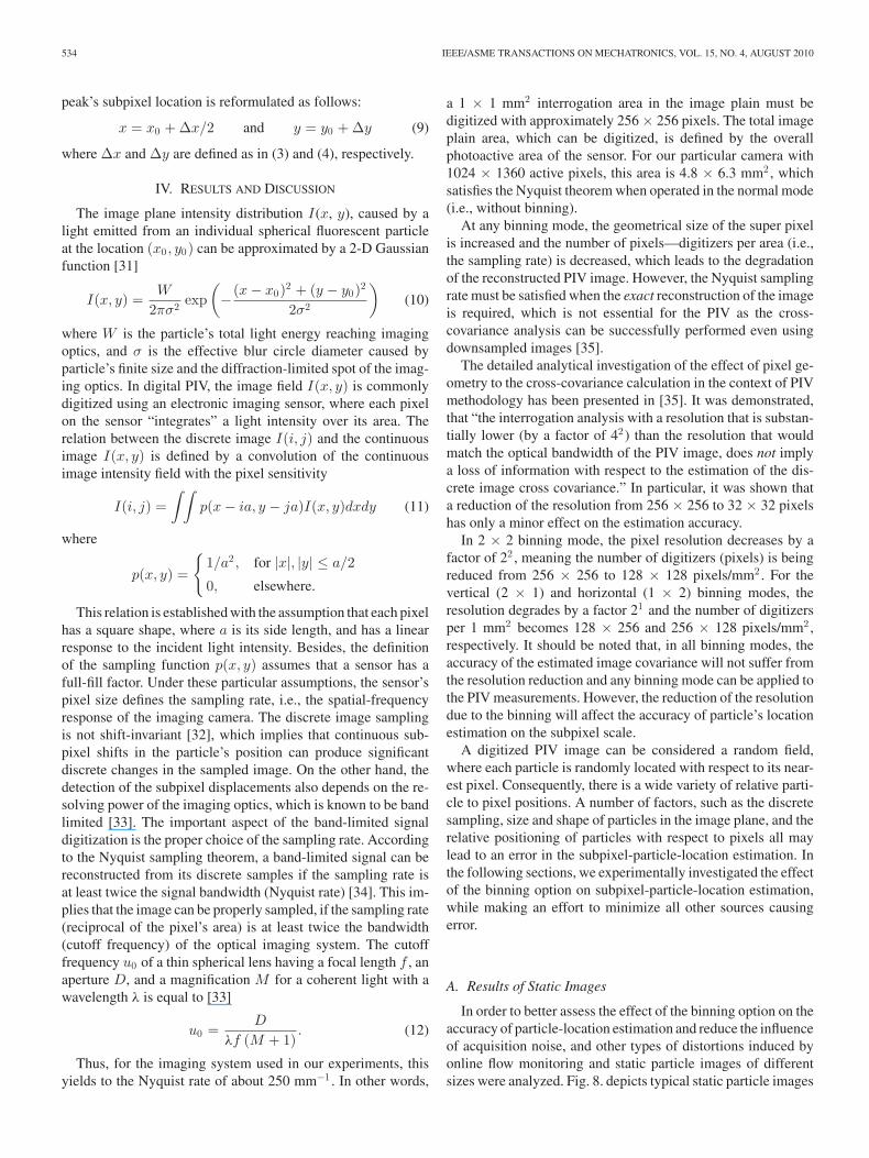
In order to study the effects of the particle’s size on the accu-racy of the particle location estimation in the context of binning,we have analyzed images with particle diameters of 0.5, 1, and1.9 µm. Additionally, to shed light upon the errors introducedby CCD binning, we analyzed errors along each axis separately,as binning may differently effect displacement estimation alongeach axis. Fig. 9 depicts the probability density functions (pdf)of bias error in x- and y-axes, and Euclidian distances for 0.5,1, and 1.9 µm diameter particles. Each pdf is estimated by nor-malizing its corresponding bias error distribution to the samplenumber. The shape of a bias error’s pdf significantly depends onthe corresponding particle size analyzed, which is as expected.

The effective diameter de of the particle projected onto theCCD imaging plane, which is the convolution of the particle’sgeometric image and the diffraction spot of imaging optics [31],can be calculated using

de =√

M 2d2p + d2

s (16)

where ds = 2.44(M + 1)λf/D is the diameter of thediffraction-limited spot (Airy function), and dp is the particle’sdiameter in the object plane. In general, PIV measurement re-sults strongly depend on the ratio of the effective particle diam-eter to the pixel size r = de/a. For the Gaussian peak fit, thebias error exhibits an inverse proportionality to the r if r < 2,and its dependency on r practically vanishes if r ≥ 2 [37].

In our experiments, for the 0.5 µm particles, we have r ≈ 1in the 2 × 2 binning mode and r ≈ 2 in the normal mode. Fol-lowing [37], we can say that the discretization of the particleimage in the 2 × 2 binning mode suffers from “serious under-sampling,” while in normal mode, the particle-image samplingis satisfactory for the subpixel peak estimation. Thus, due to theserious undersampling in the 2 × 2 binning mode, the probabil-ity of the appearance of random correlation peaks even in theinteger pixel scale will be pronounced, which is apparent in thecorresponding Fig. 9(a).

Fig. 10(a) shows a schematic representation of a “seriousundersampling” case for 2 × 2 binning, where the large solidsquares depict the 2 × 2 binned super pixels, small dashedsquares show normal pixels, and circles with their centersmarked by crosses represent particles. Depending on the fillfactor, the SNR, etc., both particles can be locked to any of thesuper pixels surrounding them. In the “worst” case, the first par-ticle could be locked to the lowest and leftmost super pixel andthe second particle to the upper rightmost super pixel. Then, thepossible maximum difference in distance between two particlescalculated in the binning and normal modes can reach about fivenormal pixels (taking into account the possible subpixel errorsas well). As can be seen from Fig. 9(a), the bias error distribution

536 IEEE/ASME TRANSACTIONS ON MECHATRONICS, VOL. 15, NO. 4, AUGUST 2010

Fig. 9. PDF of bias errors of the 2 × 2 binning mode for the particles with diameters of: (a) 0.5 µm, (b) 1 µm, (c) 1.9 µm, where x-axis (blue circles), y-axis(green crosses), and Euclidian displacement (red points).

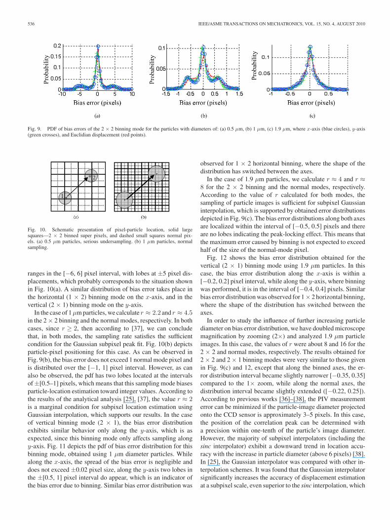
Fig. 10. Schematic presentation of pixel-particle location, solid largesquares—2 × 2 binned super pixels, and dashed small squares normal pix-els. (a) 0.5 µm particles, serious undersampling. (b) 1 µm particles, normalsampling.

ranges in the [−6, 6] pixel interval, with lobes at ±5 pixel dis-placements, which probably corresponds to the situation shownin Fig. 10(a). A similar distribution of bias error takes place inthe horizontal (1 × 2) binning mode on the x-axis, and in thevertical (2 × 1) binning mode on the y-axis.

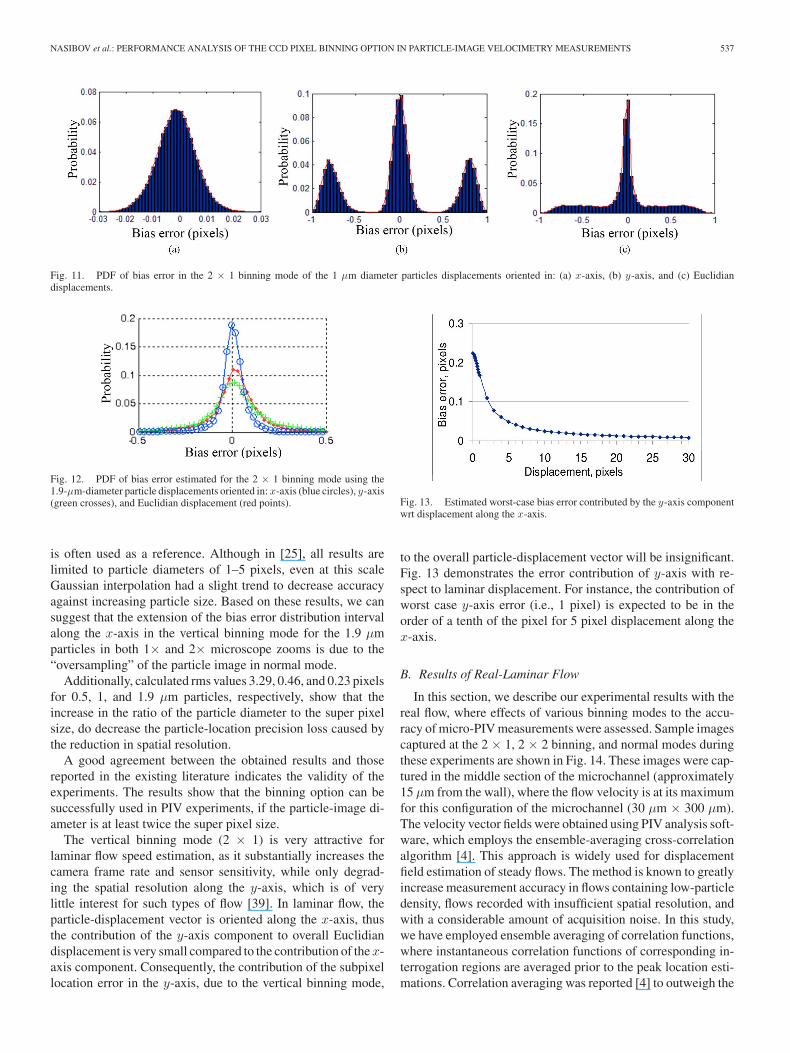
In the case of 1 µm particles, we calculate r ≈ 2.2 and r ≈ 4.5in the 2 × 2 binning and the normal modes, respectively. In bothcases, since r ≥ 2, then according to [37], we can concludethat, in both modes, the sampling rate satisfies the sufficientcondition for the Gaussian subpixel peak fit. Fig. 10(b) depictsparticle-pixel positioning for this case. As can be observed inFig. 9(b), the bias error does not exceed 1 normal mode pixel andis distributed over the [−1, 1] pixel interval. However, as canalso be observed, the pdf has two lobes located at the intervalsof ±[0.5–1] pixels, which means that this sampling mode biasesparticle-location estimation toward integer values. According tothe results of the analytical analysis [25], [37], the value r ≈ 2is a marginal condition for subpixel location estimation usingGaussian interpolation, which supports our results. In the caseof vertical binning mode (2 × 1), the bias error distributionexhibits similar behavior only along the y-axis, which is asexpected, since this binning mode only affects sampling alongy-axis. Fig. 11 depicts the pdf of bias error distribution for thisbinning mode, obtained using 1 µm diameter particles. Whilealong the x-axis, the spread of the bias error is negligible anddoes not exceed ±0.02 pixel size, along the y-axis two lobes inthe ±[0.5, 1] pixel interval do appear, which is an indicator ofthe bias error due to binning. Similar bias error distribution was

observed for 1 × 2 horizontal binning, where the shape of thedistribution has switched between the axes.

In the case of 1.9 µm particles, we calculate r ≈ 4 and r ≈8 for the 2 × 2 binning and the normal modes, respectively.According to the value of r calculated for both modes, thesampling of particle images is sufficient for subpixel Gaussianinterpolation, which is supported by obtained error distributionsdepicted in Fig. 9(c). The bias error distributions along both axesare localized within the interval of [−0.5, 0.5] pixels and thereare no lobes indicating the peak-locking effect. This means thatthe maximum error caused by binning is not expected to exceedhalf of the size of the normal-mode pixel.

Fig. 12 shows the bias error distribution obtained for thevertical (2 × 1) binning mode using 1.9 µm particles. In thiscase, the bias error distribution along the x-axis is within a[−0.2, 0.2] pixel interval, while along the y-axis, where binningwas performed, it is in the interval of [−0.4, 0.4] pixels. Similarbias error distribution was observed for 1× 2 horizontal binning,where the shape of the distribution has switched between theaxes.

In order to study the influence of further increasing particlediameter on bias error distribution, we have doubled microscopemagnification by zooming (2×) and analyzed 1.9 µm particleimages. In this case, the values of r were about 8 and 16 for the2 × 2 and normal modes, respectively. The results obtained for2 × 2 and 2 × 1 binning modes were very similar to those givenin Fig. 9(c) and 12, except that along the binned axes, the er-ror distribution interval became slightly narrower [−0.35, 0.35]compared to the 1× zoom, while along the normal axes, thedistribution interval became slightly extended ([−0.22, 0.25]).According to previous works [36]–[38], the PIV measurementerror can be minimized if the particle-image diameter projectedonto the CCD sensor is approximately 3–5 pixels. In this case,the position of the correlation peak can be determined witha precision within one-tenth of the particle’s image diameter.However, the majority of subpixel interpolators (including thesinc interpolator) exhibit a downward trend in location accu-racy with the increase in particle diameter (above 6 pixels) [38].In [25], the Gaussian interpolator was compared with other in-terpolation schemes. It was found that the Gaussian interpolatorsignificantly increases the accuracy of displacement estimationat a subpixel scale, even superior to the sinc interpolation, which

NASIBOV et al.: PERFORMANCE ANALYSIS OF THE CCD PIXEL BINNING OPTION IN PARTICLE-IMAGE VELOCIMETRY MEASUREMENTS 537

Fig. 11. PDF of bias error in the 2 × 1 binning mode of the 1 µm diameter particles displacements oriented in: (a) x-axis, (b) y-axis, and (c) Euclidiandisplacements.

Fig. 12. PDF of bias error estimated for the 2 × 1 binning mode using the1.9-µm-diameter particle displacements oriented in: x-axis (blue circles), y-axis(green crosses), and Euclidian displacement (red points).

is often used as a reference. Although in [25], all results arelimited to particle diameters of 1–5 pixels, even at this scaleGaussian interpolation had a slight trend to decrease accuracyagainst increasing particle size. Based on these results, we cansuggest that the extension of the bias error distribution intervalalong the x-axis in the vertical binning mode for the 1.9 µmparticles in both 1× and 2× microscope zooms is due to the“oversampling” of the particle image in normal mode.

Additionally, calculated rms values 3.29, 0.46, and 0.23 pixelsfor 0.5, 1, and 1.9 µm particles, respectively, show that theincrease in the ratio of the particle diameter to the super pixelsize, do decrease the particle-location precision loss caused bythe reduction in spatial resolution.

A good agreement between the obtained results and thosereported in the existing literature indicates the validity of theexperiments. The results show that the binning option can besuccessfully used in PIV experiments, if the particle-image di-ameter is at least twice the super pixel size.

The vertical binning mode (2 × 1) is very attractive forlaminar flow speed estimation, as it substantially increases thecamera frame rate and sensor sensitivity, while only degrad-ing the spatial resolution along the y-axis, which is of verylittle interest for such types of flow [39]. In laminar flow, theparticle-displacement vector is oriented along the x-axis, thusthe contribution of the y-axis component to overall Euclidiandisplacement is very small compared to the contribution of the x-axis component. Consequently, the contribution of the subpixellocation error in the y-axis, due to the vertical binning mode,

Fig. 13. Estimated worst-case bias error contributed by the y-axis componentwrt displacement along the x-axis.

to the overall particle-displacement vector will be insignificant.Fig. 13 demonstrates the error contribution of y-axis with re-spect to laminar displacement. For instance, the contribution ofworst case y-axis error (i.e., 1 pixel) is expected to be in theorder of a tenth of the pixel for 5 pixel displacement along thex-axis.

B. Results of Real-Laminar Flow

In this section, we describe our experimental results with thereal flow, where effects of various binning modes to the accu-racy of micro-PIV measurements were assessed. Sample imagescaptured at the 2 × 1, 2 × 2 binning, and normal modes duringthese experiments are shown in Fig. 14. These images were cap-tured in the middle section of the microchannel (approximately15 µm from the wall), where the flow velocity is at its maximumfor this configuration of the microchannel (30 µm × 300 µm).The velocity vector fields were obtained using PIV analysis soft-ware, which employs the ensemble-averaging cross-correlationalgorithm [4]. This approach is widely used for displacementfield estimation of steady flows. The method is known to greatlyincrease measurement accuracy in flows containing low-particledensity, flows recorded with insufficient spatial resolution, andwith a considerable amount of acquisition noise. In this study,we have employed ensemble averaging of correlation functions,where instantaneous correlation functions of corresponding in-terrogation regions are averaged prior to the peak location esti-mations. Correlation averaging was reported [4] to outweigh the

538 IEEE/ASME TRANSACTIONS ON MECHATRONICS, VOL. 15, NO. 4, AUGUST 2010

Fig. 14. Real-flow images captured at: (a) 2 × 1 vertical binning mode,(b) 2 × 2 binning mode, (c) normal mode, and (d) part of the ensemble-averagedvelocity vector field at 2 × 1 binning mode.

performance of other proposed averaging methods and is lesssensitive to erroneous flow measurements.

In general, the measurement uncertainties of PIV and micro-PIV are the same, except for those arising from the differencein illumination techniques, namely sheet and volume illumina-tions. The major source of error in micro-PIV is the definition ofthe depth of field. In the micro-PIV literature, there are discrep-ancies between definitions for the depth of field of an imagingmicrospore. In our calculations, we have used the equation de-scribed in [40]

δzm =3nλ

NA2 +2.16dp

tan θ+ dp (17)

where n is the refractive index of the medium and NA is thenumerical aperture of the objective lens. The depth of field cal-culated according to (17) is equal to 2.7 µm. This value indicatesthat the intensity contributed by particles out of this focus depthhas a negligible influence on the correlation function. The sizeof the interrogation windows were 80 × 20, 40 × 10, and 80 ×10 pixels for normal, 2 × 2, and 2 × 1 vertical binning modes,respectively. Consequently, interrogation volumes in the flowcoordinates were the same for all binning modes and equal to23.25 µm × 5.8 µm × 2.7 µm. The interrogation spots wereoverlapped by 50% to satisfy the Nyquist sampling criteria,which corresponds to 2.4 µm vector-to-vectors spacing in thestreamwise normal direction.

In the normal mode, a 1 µm particle was resolved by ap-proximately 4 pixels, which is in accord with the minimumrequirement (3–4 pixels) essential to obtain the location of aparticle-image correlation peak within one tenth of the parti-cle’s image diameter [14]. Accordingly, the measurement un-certainty can be determined using dx ≈ de/10M , which yields0.14 µm for our experiments. For a velocity of 0.7 mm/s and atime between two frames of 0.05 s, the error was evaluated tobe approximately 0.7%.

The errors due to particle diffusion caused by Brownian mo-tion along the x-direction is given by [13], εB =

√2D/(u2∆t),

where D is the Brownian diffusion coefficient. For the cur-rent experiments, with the characteristic flow velocity of

Fig. 15. Ensemble-averaged and streamwise-averaged velocity profiles at dif-ferent binning modes of two flows with 0.7 mm/s (bottom) and 1.2 mm/s (top)velocities. The bottom inset depicts the standard deviation between normal,2 × 2, and 2 × 1 binning modes.

u ≈ 0.7 mm/s and ∆t = 0.05 s, this approximately yields a0.5% relative error due to the Brownian motion.

The stability of the system, including the syringe drive pump,was estimated using the standard deviation of mean veloci-ties, calculated using the central part of the velocity profilesof different PIV measurement cycles. The stability was foundto be within 2% of the maximum mean velocity of the normalmode.

Real-flow PIV experiments were divided into cycles, whereeach cycle was performed in three stages: 1) beginning stage,where the flow images are captured using normal camera mode;2) middle stage, where the camera is immediately turned into thedesired binning mode for capturing binning images; and 3) stop-ping stage in which the camera is again returned to the normalmode, where flow images again are captured. The flow velocityfield in each stage was evaluated using ensemble averaging of20 instantaneous measurements. Fig. 14(d)) depicts ensemble-averaged mean velocity vector fields at 1.2 mm/s flow rate, cal-culated using 2 × 1 binning mode. Regions in the instantaneousfields, where valid vectors could not be obtained were excludedfrom the averaging calculation. In the same way, if the varia-tion of the mean velocities between the beginning and stoppingstages was more than 2%, the whole cycle was excluded fromfurther calculations. Finally, the streamwise velocity profileswere estimated by line averaging in the streamwise direction ofthe measured velocity data of each stage in the cycle. Fig. 15depicts the averaged velocity profiles, obtained at normal, 2 ×1, and 2 × 2 binning modes of the dataset with the maximumvelocities of 0.7 and 1.2 mm/s. Since the microscope’s FOVcould not cover the whole channel width, the velocity profilesare presented in parts.

The bottom inset in Fig. 15 shows the standard deviationbetween three mean velocities obtained at normal, 2 × 1, and2 × 2 binning modes. The variation between mean velocitiesof the three binning modes does not exceed 1.5% at 0.7 mm/sand 2% at 1.2 mm/s. These results show that the errors resultingfrom the reduction of spatial resolution in the binning option donot exceed the overall inherent error of PIV measurements.

NASIBOV et al.: PERFORMANCE ANALYSIS OF THE CCD PIXEL BINNING OPTION IN PARTICLE-IMAGE VELOCIMETRY MEASUREMENTS 539

In particular experimental conditions, the maximum measur-able velocity in the normal mode was about 1.2 mm/s, whereasin the 2 × 1 and 2 × 2 binning modes, this was raised up to avelocity of 1.9 mm/s.

Finally, in the context of PIV experiments, the CCD readouttime constitutes the overall delay between frames and limits thedynamic velocity range of measurements. In recent years, toovercome this limitation, double-frame (frame-straddled) cam-eras have been widely used [41], [42], where two frames arecaptured with a delay of a few microseconds. After exposure,the first frame is immediately shifted to the camera’s internalmemory, leaving the sensor to capture the second frame, so theexposure time of the second frame is defined by the readout timeof the first frame. Finally, the second frame is transferred to theoutput. While this technology allows minimizing the delay be-tween two straddled frames down to microseconds, the overalltime between two pairs of consecutive straddled-frames is abouttwice the sensor’s readout time. If applied, the binning optionwill reduce the readout time of each straddled frames by a factorof two, consequently, the double-frame rate will increase by afactor of four.

Additionally, the measurement techniques described in thispaper can be applied to CMOS-based imagers, where the bin-ning option is also available. However, further research is re-quired to thoroughly assess its benefits in the presence of addi-tional noise, which is caused by the binning process of CMOSimagers [43]. A wide investigation into the influence of theCCD binning option on the overall performance of CMOS anddouble-frame CCD cameras will be published elsewhere.

V. SUMMARY AND CONCLUSION

We have proposed a convenient method to increase the dy-namic velocity range in PIV measurements, which employs aCCD camera binning option. Although the binning proceduredecreases spatial resolution along specified dimensions, its abil-ity to considerably increase the camera frame rate and preservethe FOV are important features, which can be used for boostingthe dynamic velocity range. CCD binning increases the SNR andsensor sensitivity, which is very attractive in low-illuminationPIV measurements. Besides, the particle motion blur, which de-pends on the exposure time, will be reduced compared to thenormal mode, as binning mode requires less exposure time. Thesize of output image files is reduced, due to the decrease inthe number of pixels caused by binning, which allows 1) theallocation of more image files in the computer memory duringmeasurements and 2) a decrease in the amount of correlationcalculations.

Experimental and analytical results were performed on static-and real-flow images in order to demonstrate the soundness andapplicability of the proposed technique. The accuracy of themethod was demonstrated using static images of 0.5, 1, and1.9 µm diameter particles captured at various binning modes,where obtained results were in accord with results reported inthe up-to-date literature. We have shown that when the particle-image size is at least twice the size of the super pixel, thedifference between the distances estimated in normal and corre-

sponding binning modes are in the order of a tenth of a pixel’ssize.

Likewise, results obtained for micro-PIV measurements ofthe real-laminar flow inside a rectangular microchannel with1 µm diameter particles showed that the errors due to the bin-ning mode do not exceed the overall inherent errors of PIV. Inparticular experimental conditions, the maximum measurablevelocity in the normal mode was about 1.2 mm/s, whereas inthe 2 × 1 and 2 × 2 binning modes, this was raised up to avelocity of about 1.9 mm/s.

Finally, it was shown that the 2 × 1 binning mode is the mostappropriate method to increase dynamic velocity range in lam-inar flow measurements, as it increases camera frame rate andsensor sensitivity at the expense of loosing spatial resolutiononly along the vertical direction, which is of very subtle interestin such measurements. Besides, 2 × 2 binning mode, which in-creases sensor sensitivity even more, is also of great interest forflow measurements, especially in low-light illumination condi-tions; however, in this case, particles of adequate size must beused to assure measurement accuracy.

ACKNOWLEDGMENT

The authors would like to thank the three anonymous refereesfor useful comments and constructive suggestions.

REFERENCES

[1] R. J. Adrian, “Twenty years of particle image velocimetry,” Exp. Fluids,vol. 39, pp. 159–169, 2005.

[2] E. Willert and M. Gharib, “Digital particle image velocimetry,” Exp.Fluids, vol. 10, pp. 181–193, 1991.

[3] K. Prasad, R. J. Adrian, C. C. Landreth, and P. W. Offutt, “Effect ofresolution on the speed and accuracy of particle image velocimetry inter-rogation,” Exp. Fluids, vol. 13, pp. 105–116, 1992.

[4] C. D. Meinhart, S. T. Wereley, and J. G. Santiago, “A PIV algorithm forestimating time-averaged velocity fields,” Trans. ASME, J. Fluids Eng.,vol. 122, pp. 285–289, 2000.

[5] F. Scarano, “Iterative image deformation methods in PIV,” Meas. Sci.Technol., vol. 13, pp. R1–R19, 2002.

[6] H. Nasibov and S. Baytaroglu, “Recent advances in digital particle imagevelocimetry methods for flow motion analysis,” Int. J. Metrol. QualityEng., vol. 1, pp. 21–29, 2010.

[7] A. K. Prasad, “Particle image velocimetry,” Current Sci., vol. 79, no. 1,pp. 51–60, 2000.

[8] Y. Hassan and R. Canaan, “Full-field bubbly flow velocity measurementsusing a multiframe particle tracking technique,” Exp. Fluids, vol. 12,pp. 49–60, 1991.

[9] T. Uemura, F. Yamamoto, and K. Ohmi, “A high speed algorithm ofimage analysis for real time measurement of two-dimensional velocitydistribution,” in Flow Visualization, B. Khalighi, M. Braun, and C. Freitas,Eds. New York: ASME, 1989, pp. 129–133.

[10] P. Ruhnau, C. Guetter, T. Putze, and C. Schnorr, “A variational approachfor particle tracking velocimetry,” Meas. Sci. Technol., vol. 16, pp. 1449–1458, 2005.

[11] R. D. Keane, R. J. Adrian, and Y. Zhang, “Super resolution particle imagevelocimetry,” Meas. Sci. Technol., vol. 6, pp. 754–768, 1995.

[12] M. R. Bown, J. M. MacInnes, R. W. K. Allen, and W. B. J.Zimmerman, “Three-dimensional, three-component velocity measure-ments using stereoscopic micro-PIV and PTV,” Meas. Sci. Technol.,vol. 17, pp. 2175–2185, 2006.

[13] J. G. Santiago, S. T. Wereley, C. D. Meinhart, D. J. Beebe, and R. J. Adrian,“A particle image velocimetry system for microfluidics,” Exp. Fluids,vol. 25, pp. 316–319, 1998.

[14] C. D. Meinhart, S. T. Wereley, and J. G. Santiago, “PIV measurements ofa microchannel flow,” Exp. Fluids, vol. 27, pp. 414–419, 1999.

540 IEEE/ASME TRANSACTIONS ON MECHATRONICS, VOL. 15, NO. 4, AUGUST 2010

[15] S. Devasenathipathy, J. G. Santiago, S. T. Wereley, C. D. Meinhart, andK. Takehara, “Particle imaging techniques for microfabricated fluidic sys-tems,” Exp. Fluids, vol. 34, pp. 504–514, 2003.

[16] D. Erickson and D. Li, “Integrated microfluidic devices,” Anal. ChimicaActa, vol. 507, pp. 11–26, 2004.

[17] S. D. Peterson, M. Porfiri, and A. Rovardi, “A particle image velocimetrystudy of vibrating ionic polymer metal composites in aqueous environ-ments,” IEEE/ASME Trans. Mechatronics, vol. 14, no. 4, pp. 474–483,Aug. 2009.

[18] M. Hagsater, C. H. Westergaard, H. Bruus, and J. P. Kutter, “Investigationson LED illumination for micro-PIV including a novel front-lit configura-tions,” Exp. Fluids, vol. 44, pp. 211–219, 2008.

[19] O. Chetelat and K. C. Kim, “Miniature particle image velocimetry systemwith LED in-line illumination,” Meas. Sci. Technol., vol. 13, pp. 1006–1013, 2002.

[20] R. D. Keane and R. J. Adrian, “Theory of cross-correlation analysis ofPIV images,” Appl. Sci. Res., vol. 49, pp. 191–215, 1992.

[21] R. J. Adrian, “Dynamic ranges of velocity and spatial resolution of particleimage velocimetry,” Meas. Sci. Technol, vol. 8, pp. 1393–1398, 1997.

[22] J. R. Janesick, Scientific Charge-Coupled Devices. Washington, DC:SPIE Optical Engineering Press, 2001.

[23] B. F. Alexander and K. C. Ng, “Elimination of systematic error in subpixelaccuracy centroid estimation,” Opt. Eng., vol. 30, no. 9, pp. 1320–1331,1991.

[24] M. R. Cholemari, “Modeling and correction of peak-locking in digitalPIV,” Exp. Fluids, vol. 42, pp. 913–922, 2007.

[25] H. Nobach, N. Damaschke, and C. Tropea, “High-precision sub-pixel in-terpolation in particle image velocimetry image processing,” Exp. Fluids,vol. 39, pp. 299–304, 2005.

[26] T. Roesgen, “Optimal subpixel interpolation in particle image velocime-try,” Exp. Fluids, vol. 35, pp. 252–256, 2003.

[27] H. Nobach and M. Honkanen, “Two-dimensional gaussian regression forsub-pixel displacement estimation in particle image velocimetry or particleposition estimation in particle tracking velocimetry,” Exp. Fluids, vol. 38,pp. 511–515, 2005.

[28] M. Raffel, C. E. Willert, S. T. Wereley, and J. Kompenhans, Particle ImageVelocimetry: A Practical Guide, 2nd ed. Berlin: Springer-Verlag, 2007.

[29] R. P. Heilbronner, “The autocorrelation function: An image processingtoolfor fabric analysis,” Tectonophysics, vol. 212, pp. 351–370, 1992.

[30] N. Lins, “Textural image processing on granular structures of metal shad-owing replicas,” Ultramicroscopy, vol. 12, pp. 185–200, 1984.

[31] R. J. Adrian and C. S. Yao, “Development of pulsed laser velocimetry formeasurement of fluid flow,” in Proc. Eighth Biennial Symp. Turbulence,G. Patterson and J. L. Zakin, Eds. Rolla, MO: Univ. Missouri, 1983.

[32] S. K. Park, R. Schowengerdt, and M. Kaczynski, “Modulation-transfer-function analysis for sampled image systems,” Appl. Opt., vol. 23,pp. 2572–2582, 1984.

[33] J. W. Goodman, Introduction lo Fourier Optics. New York: McGraw-Hill, 1968.

[34] A. V. Oppenheim, A. S. Willsky, and I. T. Young, Signals and Systems.Englewood Cliffs, NJ: Prentice-Hall, 1983.

[35] J. Westerweel, “Analysis of PIV interrogation with low pixel resolution,”in Proc. SPIE-2005, Optical Diagnostics in Fluid and Thermal Flow,S. S. Cha and J. D. Trolinger, Eds. San Diego, CA, Jul. 14–16, 1993,pp. 624–635.

[36] H. Huang, D. Dabiri, and M. Gharib, “On errors of digital particle imagevelocimetry,” Meas. Sci. Technol., vol. 8, pp. 1427–1440, 1997.

[37] J. Westerweel, “Effect of sensor geometry on the performance of PIV in-terrogation,” in Laser Techniques Applied to Fluid Mechanics, R. J. Adrianet al., Ed. Berlin, Germany: Springer-Verlag, 2000, pp. 37–55.

[38] T. Astarita and G. Cardone, “Analysis of interpolation schemes for imagedeformation methods in PIV,” Exp. Fluids, vol. 38, pp. 233–243, 2005.

[39] B. Akselli, A. Kholmatov, and H. Nasibov, “The use of CCD pixel binningin PIV measurements,” in Proc. Optomechatronic Technol., 2009, Int.Symp. Optomechantronic Technol., pp. 223–228.

[40] C. D. Meinhart, S. T. Wereley, and M. H. B. Gray, “Volume illuminationfor two-dimensional particle image velocimetry,” Meas. Sci. Technol.,vol. 11, pp. 809–814, 2000.

[41] M. Honkanen and H. Nobach, “Background extraction from double-framePIV images,” Exp. Fluids, vol. 38, pp. 348–362, 2005.

[42] R. Hain and C. J. Kahler, “Fundamentals of multiframe particle imagevelocimetry (PIV),” Exp. Fluids, vol. 42, pp. 575–587, 2007.

[43] Z. Zhou, B. Pain, and E. R. Fossum, “Frame-transfer CMOS active pixelsensor with pixel binning,” IEEE Trans. Electron. Devices, vol. 44, no. 10,pp. 1764–1768, Oct. 1997.

Humbat Nasibov received the B.S. and M.Sc. de-grees from Baku State University, Baku, Azerbaijan,in 1990 and 1992, respectively, both in physics, andthe Ph.D. degree in experimental physics from theInstitute of Photoelectronics, Academy of Sciencesof Azerbaijan, Baku, in 2000.

From 1992 to 2001, he was an Optical Engineerat the Institute of Photoelectronics. From 2001 to2004, he was a Senior Researcher in the TemperatureStandards Laboratory, National Metrology Institute,Gebze, Turkey. In 2004, he joined the National Re-

search Institute of Electronics and Cryptology, Gebze, Turkey, where he iscurrently a Chief Senior Researcher in the Optoelectronics Department. His re-search interests include laser physics and optical spectroscopy, optoelectronics,and optical imaging metrology.

Alisher Kholmatov was born in Dushanbe,Tajikistan. He received the B.S. degree in computerengineering from Middle East Technical University,Ankara, Turkey, in 1997, and the M.Sc. and Ph.D.degrees in electronics engineering and computer sci-ence from Sabanci University, Istanbul, Turkey, in2003 and 2008, respectively.

Since 2008, he has been a Senior Researcher in theOptoelectronics Department, National Research In-stitute of Electronics and Cryptology, Gebze, Turkey.His research interests include image processing, pat-

tern recognition, and machine learning.

Basak Akselli received the B.S. and M.Sc. degreesin chemical engineering from Istanbul TechnicalUniversity, Istanbul, Turkey, in 1993 and 1997, re-spectively. She is currently working toward the Ph.D.degree in the Department of Mechanical Engineer-ing, Yildiz Technical University, Istanbul.

She is also a Researcher in the Fluid Mechan-ics Laboratory, National Metrology Institute, Gebze,Turkey. Her research interests include flow measure-ment techniques and metrology.

Adalat Nasibov received the B.S. and M.Sc. de-grees from the Moscow Engineering Physics Insti-tute, Moscow, Russia, in 1992 and 1994, respectively.

He is currently a Software Engineer at the Na-tional Research Institute of Electronics and Cryptol-ogy, Gebze, Turkey. His research interests includesignal and image processing, and control theory andapplications.

Sakir Baytaroglu received the M.Sc. degree infine mechanics and metrology engineering fromBucharest Polytechnic Institute, Bucharest, Romania,in 1985, and the Ph.D. degree from Yildiz TechnicalUniversity, Istanbul, Turkey, in 1995.

In 1985, he joined as an Assistant Researcherthe National Metrology Institute (TUBITAK UME),Gebze, Turkey. From 1988 to 1995, he was a Visit-ing Researcher at the French Metrological InstituteCNAM-INM, LNE, German Metrological InstitutePTB, and BIPM. In 1995, he joined as a Senior Re-

searcher the Turkish Aerospace Industry, Ankara, Turkey. From September 1996to 2004, he was a Technical Adviser and Responsible for R&D at Nurol Machin-ery, Ankara, Turkey. His research interests include fundamental and mechanicalmetrology.

Dr. Baytaroglu was nominated as the Deputy Director of TUBITAK UME,responsible for technical affairs in 2005.