RESEARCH ARTICLE

Zherui Zhang Æ Ronald J. Hugo

Stereo particle image velocimetry applied to a vortex pipe flow

Received: 30 September 2004 / Revised: 9 October 2005 / Accepted: 12 October 2005 / Published online: 18 November 2005� Springer-Verlag 2005

Abstract Stereo particle image velocimetry (PIV) hasbeen employed to study a vortex generated via tangen-tial injection of water in a 2.25 inch (57 mm) diameterpipe for Reynolds numbers ranging from 1,118 to63,367. Methods of decreasing pipe-induced opticaldistortion and the PIV calibration technique are ad-dressed. The mean velocity field analyses have shownspatial similarity and revealed four distinct flow regionsstarting from the central axis of rotation to the pipe wallin the vortex flows. Turbulence statistical data andvortex core location data suggest that velocity fluctua-tions are due to the axis of the in-line vortex distorting inthe shape of a spiral.

1 Introduction

Confined vortex flows, also referred to as in-line vortexflows, exist in many different industrial applications, e.g.,flow passages in turbo-machinery, cyclone separators,and large-scale pipelines. Confined vortex flows have alsofound application in industrial processes such as com-bustion stabilization (Syred et al. 1982; Anacleto et al.2003), flow regulation (Lisk 1988; Riivet et al. 1998), heatand mass transfer enhancement (Chang and Dhir 1994,1995; Wu et al. 2000), blockage prevention in pneumaticconveying systems (Li and Tomita 1994, 2000, 2001) andbeam tube protection in nuclear fusion reactors(Pemberton et al. 2003). Consequently, understanding themechanisms of the in-line vortex flow could help in thebetter design of these devices and systems by eitheraugmenting or neutralizing the effects that the vortex has

on the flowfield. The motivation behind the researchpresented in this article is to further understand thephysics of the vortex pipe flow from the fluid dynamicperspective.

A large body of previous studies in vortex pipe flowshas been experimental in nature. Generally speaking,there are three methods used to generate a vortex pipeflow (Pruvost et al. 2000): (1) rotational methodsinvolving rotation of the test section (Taylor 1921;Talbot 1954; Grosjean et al. 1997) or rotating the endcap(s) of a cylindrical test section (Spohn et al. 1998;Stokes et al. 2001); (2) injection methods where fluid iscircumferentially fed into a cylindrical cavity from oneinlet or two opposite inlets (Vonnegut 1954; Nissan andBresan 1961; Chanaud 1963; Sato and Watanabe 2000);and (3) vane methods where an adjustable swirl plate orguide vanes are used to generate the vortex (Parchen andSteenbergen 1998; Mattner et al. 2002). The secondtangential injection mechanism was used to generate thevortex in the current investigation, which was adaptedfrom vortex whistle experiments initially conducted byVonnegut (1954). This mechanism of vortex generationis characterized by the swirl intensity (vortex strength)being directly related to the volumetric flow rate.

Velocity distributions are important while attemptingto elucidate the characteristics of vortex flows. Parchenand Steenbergen (1998) comment that common trendsare not always obvious in the velocity distributionscollected using different vortex generators. The lack ofagreement in the measured velocity distributions revealsthe complexity of vortex pipe flows, and implies thatseveral different flow regimes that are dependent on theswirling intensity and the initial and downstream con-ditions may exist for such flows. Therefore, furtherinvestigation of the velocity distributions of vortex pipeflows using new measurement techniques is desirablewhile trying to understand the physical characteristics ofthese flows.

Vortex pipe flows, especially those with strong swirlintensity, possess features including strong three dimen-sionality and flow reversal that make conventional

Z. Zhang Æ R. J. Hugo (&)Department of Mechanical and Manufacturing Engineering,The University of Calgary, 2500 University Dr. N.W.,T2N 1N4 Calgary, AB, CanadaE-mail: hugo@ucalgary.caTel.: +1-403-2202283Fax: +1-403-2828406

Experiments in Fluids (2006) 40: 333–346DOI 10.1007/s00348-005-0071-z

pressure-probe or hot-wire based velocity measurementtechniques unsuitable. This results as the aforementionedtechniques are sensitive to the direction of fluid motion,and the intrusive nature of the probes themselves inter-feres with the measured flow field, especially when usedon small-scale laboratory equipment. Particle image ve-locimetry (PIV) is a well-established nonintrusive andwhole-field measurement method (Adrian 1991; Prasadand Adrian 1993), which can obtain the velocity fieldover a relatively large plane using a quantitative flowvisualization approach. The method quantifies thevelocities of fluid elements indirectly by measuring thevelocity of tiny tracer particles suspended in the investi-gated fluid. Numerous examples describing the principlesand limitations of PIV can be found in the literature(Keane and Adrian 1990, 1991; Prasad and Adrian 1993;Adrian 1997; Huang et al. 1997; Soloff et al. 1997;Stanislas and Monnier 1997; Westerweel 1997; Raffelet al. 2000; Reuss et al. 2002). In recent years, a numberof investigators have applied two-dimensional PIV toconfined vortex flows (Grosjean et al. 1997; Lozano et al.1999; Pruvost et al. 2000; Graftieaux et al. 2001). All ofthese investigations, with the exception of the experi-ments by Pruvost et al. (2000), used a rotation mecha-nism to induce a vortex flow within a closed cylindricalcontainer without net fluid flow. This method produceswhat is referred to as a vortex container flow in which theprimary flow is produced in the azimuthal direction anda secondary flow in the radial and axial directions.Grosjean et al. (1997) employed a combination of laser-Doppler anemometry (LDA) and digital PIV to investi-gate an unsteady vortex flow in a rotating pipe (rota-tional speed of 300 rpm), combining the high spatial andtemporal resolution of LDA with the whole-field mea-surement capability of PIV. PIV was used to measure thevelocity field and capture the precessing vortex core(PVC), a periodic movement of the swirl center awayfrom the geometric center of the pipe. The resultingprobability density function of the vortex core movementwas used to correct LDA-derived turbulence statistics,enabling a more detailed and accurate decomposition ofvelocity fluctuations. Pruvost et al. (2000) applied PIV toa vortex flow generated through the tangential injectionof fluid into a 1.5-m-long annulus between two concen-tric pipes. All of the experiments were conducted at awater flow rate of Q=2.14 m3/h or Re=5,400. Theresearchers measured the three components of velocityusing a two-step acquisition process. The first acquisitionstep was made in a horizontal plane through the hori-zontally aligned centerline of the pipe, and this gave thesimultaneous axial and radial velocities in the entireannular gap width. The second acquisition step wasmade in a horizontal plane off of the center of the pipewhere the azimuthal velocity was tangent to the lasersheet at the center of the acquisition area, and this gavethe azimuthal velocity at one radial location and differ-ent axial positions. By moving the laser sheet vertically, itwas possible to investigate the azimuthal velocity atseveral radial locations.

In the current investigation, stereo digital PIV wasused to measure the three components of velocity in avortex pipe flow generated using tangential injection forReynolds number ranging from 1,118 to 63,367. Theexperimental apparatus and PIV calibration technique isdescribed in Sect. 2. Measurement results are presentedin Sect. 3, with the main conclusions presented in Sect. 4.

2 Experimental apparatus and PIV calibration

The experimental apparatus consisted of two main parts,the vortex generator assembly with associated flowpiping and the stereo PIV system with traversing hard-ware. These two main parts will be described in detail inthe following two subsections.

2.1 Vortex generator assembly

The vortex generator assembly was designed for modu-larity, enabling the assembly to be dismantled and re-placed with another design easily and quickly. A sectionview of the vortex generator assembly is depicted inFig. 1. The vortical flow was generated by feeding watertangentially into a cylindrical cavity (P8) from a tan-gential inlet tube (P9), strengthening vortex strength viacontraction into the smaller diameter test section (P6)where the velocity field measurements were performed.The vortex flow then entered a larger diameter down-stream tube, the expansion tube (P2), where pressurefluctuations of the PVC were examined in a separateinvestigation (Veer 2004). The flow discharged from theexpansion tube into a collection tank and was recircu-lated by a water pump (not shown in Fig. 1). A gatevalve was installed at the end of the expansion tube andused to adjust the discharge rate and to purge trappedair out from the bleeding hole (P11). The tubes (P6 andP2) were immersed in a 451·445·559 mm (L·W·H)water tank (P1) to minimize optical distortion caused bythe curved pipe wall and to facilitate the calibration ofthe PIV system in conjunction with a calibration plat-form (P5), which is described further in Sect. 2.3. Thewater tank was built from 0.5¢¢(13 mm) transparentPlexiglas plates. The test section (P6) and the expansiontube (P2) were made from 2.25·0.125¢¢(57·3 mm) and3.25·0.125¢¢(83·3 mm) transparent cast Plexiglas pipes,respectively. Cast pipes were used instead of extrudedpipes for improved optical quality.

2.2 Stereo PIV and its arrangement

A LaVision FlowMaster3 stereo digital PIV system wasused to perform the three-component velocity mea-surements. The system included a New Wave ResearchNd:YAG pulsed laser, Solo III-15, with 50 mJ maxi-mum energy output at 532 nm and 15 Hz repetitionrate. The CCD cameras used SONY ICX 085 arrays

334

with 12-bit dynamic range, 1280·1024 pixels resolution,and 6.7 lm·6.7 lm pixel size. The CCD cameras wereused in the double-frame/double-exposure mode with amaximum acquisition frequency of 4 Hz during theexperiments described here. The double-frame/double-exposure mode allows two recorded images, illuminatedby two sequential laser flashes, to be stored in two sep-arate frames, and the temporal order of the images wastherefore inherently registered to eliminate velocitydirection ambiguity. The seeding material consisted ofDantec polyamide seeding particles (PSP) with a meandiameter of 5 lm and density of 1.03 g/cm3. Using themethods listed in (Raffel et al. 2000), this seedingmaterial had very good fluid and imaging properties forthe current experiments, with the theoretically computed

velocity lag less than 1 lm/s and the frequency responselarger than 2.5 MHz. The particle image size was about2.5 pixels given the cameras’ working distance of about60 cm, which was within the 2–3 pixel optimal size forthe PIV evaluation algorithm, as specified by the sys-tem’s manufacturer.

The arrangement of the two cameras and the laserwas determined by the limited optical access to the testsection. In preliminary experiments, a vertically alignedlaser light sheet was used to illuminate the test sectionthrough the side of the water tank in the radial direction.This configuration resulted in bright glares off of thefront and rear pipe walls. These glares had sufficientintensity in that they caused the CCD sensors to satu-rate, jeopardizing their safety should the laser energy be

Fig. 1 Section view of thevortex generator assembly

335

increased to the required level for sufficient signalintensity from the tracer particles. The glares also de-creased the effective measurement area in the investiga-tion plane. In order to avoid these problems, the laserwas arranged to fire down through the Top Cap (P10) ofthe vortex generator through the central plane of the testsection, as illustrated in Fig. 2. The light sensed by bothcameras had almost identical intensity in this arrange-ment.

2.3 Distortion compensation and empirical calibration

According to Soloff et al. (1997), the accuracy of theparticle’s displacement measurement depends on twotypes of optical aberrations, focusing aberrations andimage distortion. In the PIV system used in the currentinvestigation, the focusing aberrations were decreasedusing the manufacturer-supplied Scheimpflug adapters,which could reduce the out-of-focus area created by thecameras’ oblique viewing directions (Prasad and Jensen1995). The image distortion, caused by the magnificationvariation in the field of the image, was inevitable withthe apparatus and required a calibration procedure tocompensate for the effects (Prasad and Adrian 1993).The main source of magnification variation was refrac-tion caused by the curved pipe wall and the water heldwithin the pipe. To help minimize refraction, a rectan-

gular Plexiglas tank (P1 in Fig. 1) was filled with waterand placed around the test section (Water Tank inFig. 2). Additionally, the test section (P6) was fabricatedusing thin-walled pipe (3 mm) in order to help minimizeerrors induced while imaging through the curved pipewall (Reuss et al. 2002).

The PIV system required a full empirical calibrationusing a standard 3-D calibration plate featuring twouniform grids, one recessed further into the plate thanthe other. The calibration plate was placed behind a halfsection of Plexiglas pipe (Fig. 3) cut from the same pipeused to build the test section (P6). The half section ofpipe was accurately positioned in a grooved slot ma-chined into the calibration platform, as illustrated inFig. 3. The slot in the calibration plate ensured that thehalf section of pipe was positioned at the same distancefrom the front wall of the Plexiglas tank as the actualtest section (P6). Once the tank was filled with water, theplane of the calibration plate simulated the opticalconditions at the central plane of the test section. Thiswas required, as it was not possible to place the cali-bration plate directly into the test section. The CCDcameras were coupled together through a rigidconnecting bar and were first placed in the calibrationposition as shown in Fig. 3, taking the calibration ima-ges. After the calibration was complete, the cameraswere translated 5.5¢¢(140 mm) laterally on a translationstage to the measurement position, as shown in Fig. 3.Care was taken to ensure that the axis of the translationstage was parallel to the front wall of the Plexiglas tank,ensuring that the distance between the cameras and thecalibration half section was the same as the distancebetween the cameras and the actual test section.

The validity of the empirical calibration was evalu-ated by computing the standard deviation of the markson the calibration plate, indicating how well the com-puted positions of crosses using the mapping functionagreed with the measured positions of crosses on the

CCD Cameras

WaterTank

Laser

Fig. 2 Arrangement of the PIV

A-A

5.5”

(140mm)

Calibration Position

Measurement Position

CalibrationPlatform

Half TestSection

Fig. 3 Calibration platform as viewed from CCD cameras

336

calibration plate. The standard deviation of marks in thecurrent experimental apparatus was about 0.5 pixels, anumber well below the maximum tolerance level ofone pixel specified by the PIV system’s manufacturer.This demonstrated that the calibration strategy used fordecreasing the optical distortion was acceptable. Furtherdetails on the calibration method can be found in Zhang(2004), and the accuracy of the calibration will be dis-cussed more in a later subsection.

3 PIV measurements and results

At each traversing station, 500 particle image data setswere collected in order to achieve a statistically con-verged mean velocity field. Measured flow rates rangedfrom 0.1 to 0.78 l/s in increments of approximately 0.2 l/s. The time separation between the two laser firingsvaried from 1,000 to 16 ls for the different flow rates, astabulated in Table 1.

A standard cross-correlation method was used toprocess the particle images for PIV evaluation, using anadaptive multi-pass algorithm with decreasing interro-gation window size from 64·64 pixels to 32·32 pixelswith 40% overlap. The spatial resolution achieved bythis algorithm was 1 mm.

The CCD cameras were only able to image 62 mm ofvertical height of the test section. In order to collect PIVdata along the entire 9¢¢(229 mm) of visible test section,it was necessary to collect data at four discrete flowpositions. This was accomplished using a verticaltranslation rail, enabling both CCD cameras to bemoved vertically in a manner that maintained their rel-ative position with respect to the test section. During thisprocess, overlapping regions were sampled betweenconsecutive flow positions in order to ensure completeflow sampling.

3.1 Mean velocity field data

Figure 4 shows a vector plot of the resulting meanvelocity field in the test section at a flow rate ofQ=2.11 l/s or Re=47,159. A scaling aspect ratio of 1:2was chosen for presentation purposes, noting that thischoice of scaling distorts the shape of the vortex core.This velocity map shows the velocity in the central planeof the test section, revealing the spatial locations of themean field flow structures.

From Fig. 4, it can be seen that axial flow reversal isconfined to the middle of the tube, enclosed by the

annular nonreversing mainstream flow that extends outto the tube wall. Two large-scale vortices with oppositerotational direction are observed residing upstream ofthe expansion at axial locations 1.5R and 7R. It isspeculated that these two vortices are connected; form-ing part of the same curved vortex line that crosses themeasurement plane twice. The curvature in the vortexline is believed to be the result of the axis of the vortextwisting in a corkscrew-shaped spiral (Leibovich 1978).If one were to perform a three-dimensional Biot–Savartintegration (Kuethe and Chow 1986) along a vortex,computing the centerline velocity induced by the helicalvortex structure, an upstream component of velocitywould be observed (Cheung 1997). It is believed that thisis the cause of the observed flow reversal in the vortexpipe flow. Inspection of all of the velocity maps collectedduring the investigation found a similar flow structure atall measured flow rates.

Figure 5 shows the mean azimuthal and axialvelocity profiles at flow rates Q=0.12 l/s (Re=2,682)and Q=1.02 l/s (Re=22,797) as a function ofstreamwise position. The thick vertical line at both

Table 1 Laser time separations at selected flow rates

Flow rate(l/s)

0.12 0.25 0.51 1.02 1.51 1.81 2.11 2.41 2.78

Time separation(ls)

600 300 160 80 40 30 25 20 16

–1 –0.5 0 0.5 10

1

2

3

4

5

6

7

8

r/R

h/R

Q=2.11L/s2.0m/s

–28.5 –14.3 0 14.3 28.5

0

28.5

57

85.5

114

142.5

171

199.5

228

Radius ( mm )

Dis

tanc

e fr

om E

xpan

sion

( m

m )

Fig. 4 Mean velocity field at Re=47,159

337

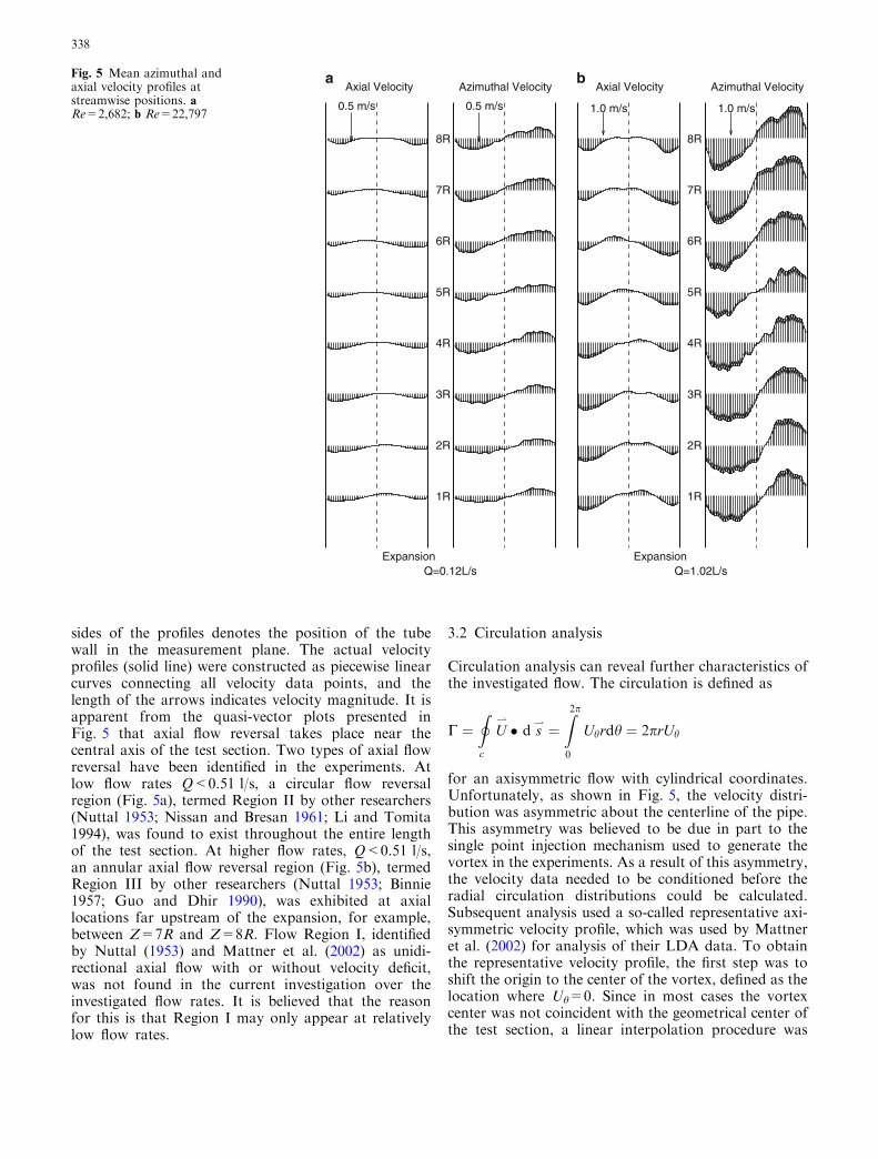
sides of the profiles denotes the position of the tubewall in the measurement plane. The actual velocityprofiles (solid line) were constructed as piecewise linearcurves connecting all velocity data points, and thelength of the arrows indicates velocity magnitude. It isapparent from the quasi-vector plots presented inFig. 5 that axial flow reversal takes place near thecentral axis of the test section. Two types of axial flowreversal have been identified in the experiments. Atlow flow rates Q<0.51 l/s, a circular flow reversalregion (Fig. 5a), termed Region II by other researchers(Nuttal 1953; Nissan and Bresan 1961; Li and Tomita1994), was found to exist throughout the entire lengthof the test section. At higher flow rates, Q<0.51 l/s,an annular axial flow reversal region (Fig. 5b), termedRegion III by other researchers (Nuttal 1953; Binnie1957; Guo and Dhir 1990), was exhibited at axiallocations far upstream of the expansion, for example,between Z=7R and Z=8R. Flow Region I, identifiedby Nuttal (1953) and Mattner et al. (2002) as unidi-rectional axial flow with or without velocity deficit,was not found in the current investigation over theinvestigated flow rates. It is believed that the reasonfor this is that Region I may only appear at relativelylow flow rates.

3.2 Circulation analysis

Circulation analysis can reveal further characteristics ofthe investigated flow. The circulation is defined as

C ¼I

c

U*� d s

* ¼Z2p

0

Uhrdh ¼ 2prUh

for an axisymmetric flow with cylindrical coordinates.Unfortunately, as shown in Fig. 5, the velocity distri-bution was asymmetric about the centerline of the pipe.This asymmetry was believed to be due in part to thesingle point injection mechanism used to generate thevortex in the experiments. As a result of this asymmetry,the velocity data needed to be conditioned before theradial circulation distributions could be calculated.Subsequent analysis used a so-called representative axi-symmetric velocity profile, which was used by Mattneret al. (2002) for analysis of their LDA data. To obtainthe representative velocity profile, the first step was toshift the origin to the center of the vortex, defined as thelocation where Uh=0. Since in most cases the vortexcenter was not coincident with the geometrical center ofthe test section, a linear interpolation procedure was

0.5 m/s 0.5 m/s

1R

2R

3R

4R

5R

6R

7R

8R

Q=0.12L/s

Axial Velocity Azimuthal Velocity

Expansion

1.0 m/s 1.0 m/s

1R

2R

3R

4R

5R

6R

7R

8R

Q=1.02L/s

Axial Velocity Azimuthal Velocity

Expansion

a bFig. 5 Mean azimuthal andaxial velocity profiles atstreamwise positions. aRe=2,682; b Re=22,797

338

used to compute an equal number of grid points (35) oneither side of the vortex center. In cases where the vortexcenter was different from the geometric center, the gridspacing was different on either side of the vortex center.In order to resolve this problem, the grid spacing wastransformed to be equal on either side of the center. Therepresentative axisymmetric velocity profile was thenobtained by calculating its azimuthal average using

�X rið Þ ¼Xh¼0 rið Þ þ Xh¼p rið Þ

2;

where �X denotes the representative axisymmetricquantities, and ri the transformed radius of the ith datapoint.

The influence of swirl on the structure of the flow canbe best illustrated by the radial circulation distribution.Figures 6, 7 and 8 show the nondimensional radial cir-culation distribution [C/(UbR)] (where Ub is the meanaxial velocity in the test section and R is the radius oftest section) at different axial locations with varyingReynolds number. In all three figures, the symbolsdenote data points and the solid lines denote the fittedcurves.

The radial circulation distribution has certain evidentcharacteristics. There are four distinguished regionsstarting from the axis of rotation to the pipe wall, withfitted curves:

Forced vortex region: �C ¼ c1�r2

Mixed vortex region: �C ¼ c2 þ c3�r2

Free vortex region: �C ¼ c4Wall region: �C ¼ c5 þ c6 log�r

where �C is the nondimensional circulation normalizedby UbR, �r the nondimensional radial location

normalized by the tube radius R, and c1, c2, c3, c4, c5 andc6 constants.

Referring to station z=4R in Fig. 6, the flow exhibitssolid body rotation for r<0.4R, forming what is referredto as the forced vortex region. The mixed vortex zoneis seen to occupy the annular region between0.4R<r<0.7R, and is so-called because it is the regionwhere the forced vortex transitions to a free vortex. Aplateau region is observed between the mixed vortexregion and the wall region within the range0.7R<r<0.9R where the circulation remains almostunchanged. This indicates an irrotational flow region,and is referred to as the free vortex region. The wallregion resides in the area close to the wall and is char-acterized by a sharp drop in circulation. The free vortexregion was observed to narrow and eventually vanishwith increasing Reynolds number. This can be found bycomparing the free vortex region at similar streamwisepositions in all three circulation distribution plots(Figs. 6, 7, 8). For Re £ 11,399, all four circulation re-gions exist throughout the entire length of the test sec-tion, as evidenced in Fig. 6. With increased Reynoldsnumbers the free vortex zone is seen to become rathernarrow or no longer exist at station z=8R for 11,399<Re £ 33,749 in Fig. 7, nor at stations z=8R and 4R for33,749< Re £ 62,134 in Fig. 8.

It is known that for the method of vortex generationused in the current experiments the swirl intensity in-creases with increased Reynolds number, as does theangular momentum. The solid body rotation or forcedvortex region was seen to gradually expand towards thepipe wall with increased Reynolds number. At the sametime, the free vortex region was seen to vanish, and athree-region profile eventually replaced the four-regionprofile along the entire test section length for sufficiently

0 0.2 0.4 0.6 0.8 10

2

4

6

8

10

12

14

16

r = r/R

Q=0.25L/s

Nor

mal

ized

Circ

ulat

ion

Γ =

Γ /(

UbR

)

Γ = 49.88r 2→

→ Γ = 36.12r 2

Γ = 1.26+28.61r 2 → →Γ = 3.02+16.14r 2

→Γ = 3.14+12.38r 2

Γ = 15.15 →

↓Γ = 11.63

↑Γ = 8

→Γ = 1.43–89.33logr

→

→Γ = 4.97–18.58logr

8R4R1R

Γ = 5.05–53.16logr

Fig. 6 Normalized radialcirculation distributions atRe=5,588

339

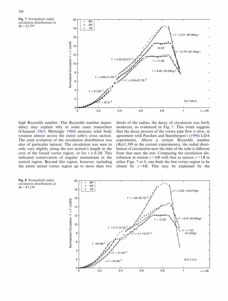
high Reynolds number. This Reynolds number depen-dency may explain why in some cases researchers(Chanaud 1963; Mattingly 1988) measure solid bodyrotation almost across the entire tube’s cross section.The axial evolution of the circulation distribution wasalso of particular interest. The circulation was seen toonly vary slightly along the test section’s length in thecore of the forced vortex region, or for r £ 0.2R. Thisindicated conservation of angular momentum in thecentral region. Beyond this region, however, includingthe entire mixed vortex region up to more than two

thirds of the radius, the decay of circulation was fairlymoderate, as evidenced in Fig. 7. This trend suggeststhat the decay process of the vortex pipe flow is slow, inagreement with Parchen and Steenbergen’s (1998) LDAexperiments. Above a certain Reynolds number(Re‡1,399 in the current experiments), the radial distri-bution of circulation near the inlet of the tube is differentfrom that near the exit. Comparing the circulation dis-tribution at station z=8R with that at station z=1R ineither Figs. 7 or 8, one finds the free vortex region to beabsent by z=8R. This may be explained by the

0 0.2 0.4 0.6 0.8 10

2

4

6

8

10

12

14

16

18

20

r = r/R

Q=1.02L/s

Nor

mal

ized

Circ

ulat

ion

Γ =

Γ /(

UbR

)

Γ = 51.93r 2→

→ Γ = 42.2r 2

Γ = 4.33+22.01r 2→

Γ = 3.66+21.04r 2 →→ Γ = 2.54+22.79r 2

↑14.59

↑Γ = 11.66

→ Γ = 5.01–90.06log r

→ Γ = 6.79–63.16log r

Γ = 6.85–35.09log r →

8R4R1R

Fig. 7 Normalized radialcirculation distributions atRe=22,797

0 0.2 0.4 0.6 0.8 10

2

4

6

8

10

12

14

16

18

20

r = r/R

Q=2.11L/s

Nor

mal

ized

Circ

ulat

ion

Γ =

Γ /(

UbR

)

Γ =65.88r 2 →

→ Γ = 54.95r 2

→ Γ = 41.43r 2

Γ = 1.49+30.72r 2→

Γ = 5.7+13.74r 2 →

→ Γ = 4.1+16.27r 2

↑Γ = 12.09

→ Γ = 0.26–134.27logr

→ Γ = 6.91–60.69logr

→ Γ = 7.33–31.52logr

8R4R1R

Fig. 8 Normalized radialcirculation distributions atRe=47,159

340

streamwise decay of angular momentum in this regionwhere the decay in circulation was pronounced. Anotherinteresting pattern in the circulation distribution was thesharp drop near the wall zone. The peak circulation inthis zone was noted to decrease in the flow direction.This suggested that friction and viscous dissipation in-duced by the presence of the pipe wall decreased theangular momentum of the fluid significantly.

3.3 Turbulence statistics

The fluctuation of velocity, uj, provides a method bywhich the magnitude of turbulence can be quantified.The intensity of velocity fluctuations can be measured bythe standard deviation (root-mean-square) of thevelocity component u

0i ¼ ui � uið Þ1=2; where i denotes the

three velocity components, c, h and z.Turbulent kinetic energy is defined as an average over

the three squared components of turbulenceintensity, that is u

02 ¼ 13 ui � ui ¼ 1

3 u02r þ u

02h þ u

02z

� �:

Figures 9 and 10 plot the three components of turbu-lence intensity and the turbulent kinetic energy at vari-ous streamwise positions for cases of both weak andstrong swirl, respectively. All of these quantities havebeen normalized by the corresponding bulk axialvelocity. The choice to normalize by the bulk axialvelocity was a difficult one as the flow is characterized bydisparate velocity scales. As an example, at a flow rate of2.11 l/s the respective mean peak-to-peak azimuthal,axial, and radial velocities divided by the bulk axialvelocity are 7.3, 3.1, and 1.9. Normalization by thesmaller bulk axial velocity leads to very high turbulence

intensities, as indicated by azimuthal values as high as500% in Fig. 10a. Normalizing the same data by meanpeak-to-peak azimuthal velocity, on the other hand,results in a maximum turbulence intensity of 68%. In theend, it was decided to normalize all three velocity com-ponents using only a single velocity value, the bulk axialvelocity.

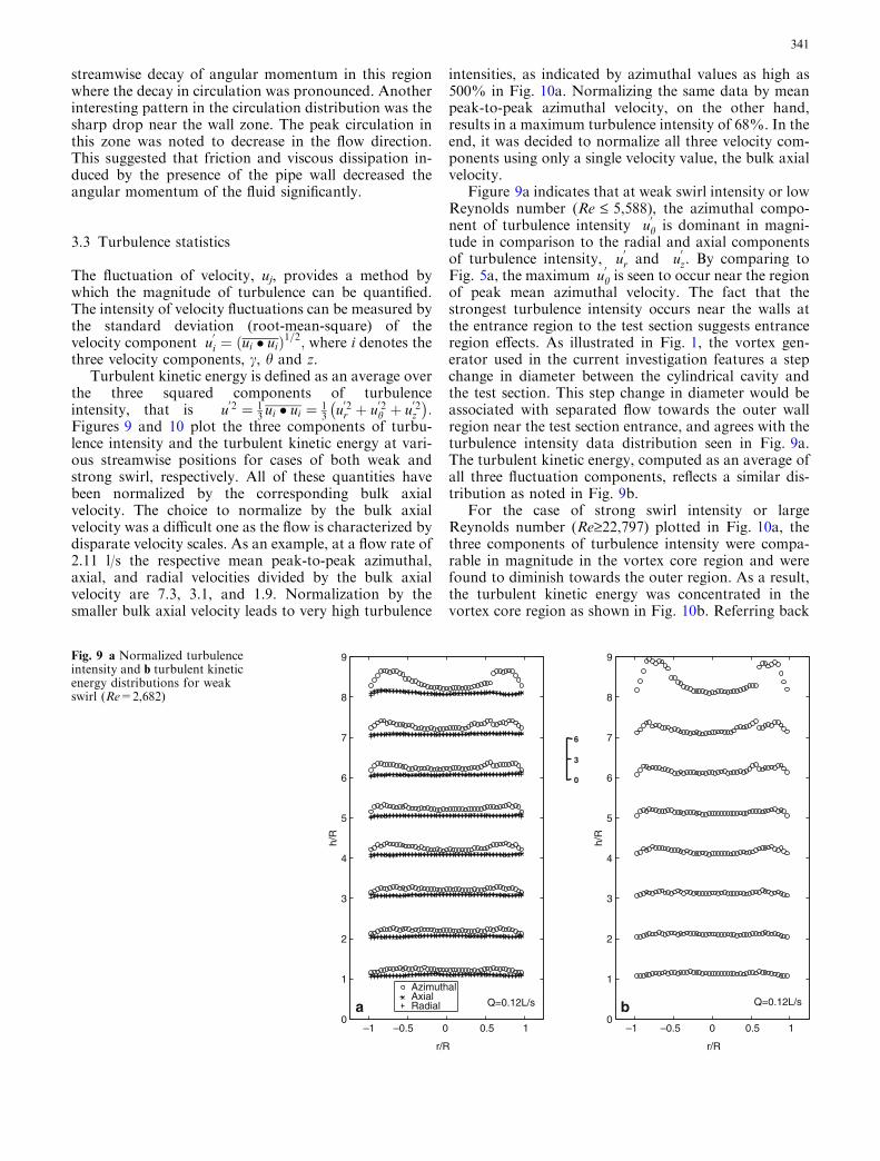
Figure 9a indicates that at weak swirl intensity or lowReynolds number (Re £ 5,588), the azimuthal compo-nent of turbulence intensity u

0

h is dominant in magni-tude in comparison to the radial and axial componentsof turbulence intensity, u

0r and u

0z. By comparing to

Fig. 5a, the maximum u0

h is seen to occur near the regionof peak mean azimuthal velocity. The fact that thestrongest turbulence intensity occurs near the walls atthe entrance region to the test section suggests entranceregion effects. As illustrated in Fig. 1, the vortex gen-erator used in the current investigation features a stepchange in diameter between the cylindrical cavity andthe test section. This step change in diameter would beassociated with separated flow towards the outer wallregion near the test section entrance, and agrees with theturbulence intensity data distribution seen in Fig. 9a.The turbulent kinetic energy, computed as an average ofall three fluctuation components, reflects a similar dis-tribution as noted in Fig. 9b.

For the case of strong swirl intensity or largeReynolds number (Re‡22,797) plotted in Fig. 10a, thethree components of turbulence intensity were compa-rable in magnitude in the vortex core region and werefound to diminish towards the outer region. As a result,the turbulent kinetic energy was concentrated in thevortex core region as shown in Fig. 10b. Referring back

–1 –0.5 0 0.5 10

1

2

3

4

5

6

7

8

9

r/R

h/R

Q=0.12L/s

AzimuthalAxialRadial

–1 –0.5 0 0.5 10

1

2

3

4

5

6

7

8

9

r/R

h/R

Q=0.12L/s

0

6

3

a b

Fig. 9 a Normalized turbulenceintensity and b turbulent kineticenergy distributions for weakswirl (Re=2,682)

341

to Fig. 4, high turbulence intensity towards the center-line can be explained by the vortex core spiraling aboutthe pipe centerline in the form of a helix. AlthoughFig. 4 was a time average, it indicates that the vortexcore is off axis most of the time. This would tend toinduce large velocity fluctuations near the centerline ofthe pipe, as observed in both Figs. 10a and b.

Relatively flat regions near the centerline of the pipein Fig. 9a and away from the centerline in Fig. 10a showthe out-of-plane azimuthal turbulence intensity to beseveral times greater than both the in-plane axial andradial components. The larger azimuthal turbulenceintensity is partially attributed to larger statistical errorsin the out-of-plane azimuthal component, shown byothers (Prasad and Adrian 1993) to be up to four timeslarger than the in-plane components, and due to the factthat the azimuthal velocity component is larger thanboth the radial and axial components, resulting in largerintensities when all three components are normalized bythe same bulk axial velocity.

An explanation for the redistribution of turbulentenergy from the outer wall region (Fig. 9) to the cen-terline of the pipe (Fig. 10) with increasing Reynoldsnumber is not obvious. It is speculated that this trendmay be attributed to the presence of a stronger vortexleading to the development of a more fully developedrecirculation zone in the upstream step region of thecylindrical cavity. Such a recirculation zone would en-able a smoother transition in the flow from the cylin-drical cavity to the test section. However, in order tofully understand this effect, an investigation of the flowinside the cylindrical cavity would be required, some-thing that was not performed during the investigation.

3.4 Vortex core locations

Turbulence statistics presented in Figs. 9 and 10 havenot been conditioned to remove the large-scale fluctua-tions induced by the motion of the vortex core from oneimage to the next, as described by Grosjean et al. (1997)in their analysis of a periodically precessing vortex core.In order to further investigate the turbulence statistics,the motion of the vortex core at each flow location wascollected by visually inspecting each set of 500 velocityfields and manually recording the position of the vortexcore in each velocity field plot. The resulting vortexposition data is shown in Fig. 11 for the case of weakswirl (Re=2,682) and in Fig. 12 for the case of strongswirl (Re=47,159) where both clockwise (CW) andcounterclockwise (CCW) vortex locations have beenindicated. The vortex location data has been separatedinto what are referred to as two distinct states, States 1and 2. In performing this separation, it was noted thatwhen all of the vortex location data was overlaid, bothCW and CCW vortices were co-located in the same re-gion of the flow. Given that the vortex is distorted in theform of a helix, it would not be possible to have twovortices of different sign in the same region of the flow atthe same time, and consequently the vortex location datawas filtered by combining CW vortex locations above150 mm with CCW vortex locations below 150 mm(State 1), and CCW vortex locations above 150 mm withCW vortex locations below 150 mm (State 2).

State 1 is characterized by vortex locations clus-tered close to the pipe centerline while State 2 showsvortex locations at a larger radial distance from thepipe centerline. State 1 was found to occur more often

–1 –0.5 0 0.5 10

1

2

3

4

5

6

7

8

9

r/R

–1 –0.5 0 0.5 1

r/R

h/R

Q=2.11L/sAzimuthalAxialRadial

0

1

2

3

4

5

6

7

8

9

h/R

Q=2.11L/s

0

10

5

a b

Fig. 10 a Normalizedturbulence intensity and bturbulent kinetic energydistributions for strong swirl(Re=47,159)

342

with an appearance frequency of 70% for weak swirland 85% for strong swirl. For all states and swirlconditions, the vortex locations were found to varymore in axial position than in radial position. Theupstream vortex location for State 1 with strong swirl(Fig. 12a) was found to have the lowest locationscatter. It was difficult to extract further information

from the vortex location data due to the fact that only62 mm of the test section’s total 229 mm verticallength could be imaged in each velocity plot. Conse-quently, it was not possible to determine informationsuch as the separation distance between a CW andCCW vortex pair, which would have further assistedin understanding the dynamics of the vortex.

–1 –0.5 0 0.5 10

1

2

3

4

5

6

7

8

r/R

h/R

Q=0.12L/s

CWCCW

–28.5 –14.3 0 14.3 28.5

0

28.5

57

85.5

114

142.5

171

199.5

228

Radius ( mm )

Dis

tanc

e fr

om E

xpan

sion

( m

m )

–1 –0.5 0 0.5 10

1

2

3

4

5

6

7

8

r/R

h/R

Q=0.12L/s

CWCCW

–28.5 –14.3 0 14.3 28.5

0

28.5

57

85.5

114

142.5

171

199.5

228

Radius ( mm )

Dis

tanc

e fr

om E

xpan

sion

( m

m )

a b

Fig. 11 Clockwise (CW) andcounterclockwise (CCW) vortexlocations for weak swirl(Re=2,682): a State 1 (70%occurrence); b State 2 (30%occurrence)

–1 –0.5 0 0.5 10

1

2

3

4

5

6

7

8

r/R

h/R

Q=2.11L/s

CWCCW

–28.5 –14.3 0 14.3 28.5

0

28.5

57

85.5

114

142.5

171

199.5

228

Radius ( mm )

Dis

tanc

e fr

om E

xpan

sion

( m

m )

–1 –0.5 0 0.5 10

1

2

3

4

5

6

7

8

r/R

h/R

Q=2.11L/s

CWCCW

–28.5 –14.3 0 14.3 28.5

0

28.5

57

85.5

114

142.5

171

199.5

228

Radius ( mm )

Dis

tanc

e fr

om E

xpan

sion

( m

m )

a b

Fig. 12 CW and CCW vortexlocations for strong swirl(Re=47,159): a State 1 (85%occurrence); b State 2 (15%occurrence)

343

A comparison of turbulence intensity in Fig. 10a andturbulent kinetic energy in Fig. 10b with vortex loca-tions in Fig. 12 reveals that flow regions with the highestturbulence intensity and energy correspond to regionswhere the vortex core often resides. This is an expectedresult as velocities in near proximity to a vortex coreshould be large. The fact that this trend does not appearfor the case of weak swirl (Figs. 9a, 11) can be explainedby the turbulence generated by entrance region effectsbeing larger than the turbulence due to the vortex.

Comparison of Fig. 10a with Fig. 12 at location 7Rreveals that the largest turbulence intensity is locatedbetween the CW and the CCW vortex cores. Closerexamination of the magnitudes in Fig. 10a shows theazimuthal component to be the largest, followed by theradial component and then the axial component. Thefact that the axial component is the smallest indicatesthat the vortex axis intersects the PIV system’s laser lightsheet at a small angle, producing the strong azimuthalcomponent.

3.5 Measurement accuracy

Two different methods were used to assess the accuracyof the PIV measurements. The first involved a compar-ison of volumetric flow rates, one measured directlyusing the flow meter installed as part of the experimentalapparatus and the second computed using the PIV-measured mean axial velocity profile. This enabled theaccuracy of the axial velocity profile to be assessed. Thesecond method used to assess the accuracy of the PIVinvolved computing the rms error between overlappingvelocity profiles collected at different vertical flow posi-tions. This enabled the repeatability of all three velocitycomponents to be assessed due to both statistical noisein the PIV-processing algorithms and post-calibrationcamera translations. Again, as with the turbulenceintensity data, the rms difference data were normalizedby the corresponding bulk axial velocity.

A comparison between measured volumetric flow rateand profile-integrated volumetric flow rate (assumingthe profile to be axisymmetric) for all tested flow rateswas performed at locations 1R, 3R, 4R, 5R, 6R, and 7Rand the respective rms errors were computed to be 16.0,11.5, 3.9, 8.8, 21.3, and 11.1%. While integrating thevelocity profiles, the two axial velocities at a commonradial distance from the origin of the pipe were averagedand used according to the axisymmetry assumption. Therms error is seen to vary significantly with flow position,with the smallest errors occurring near the middle of thetest section and the highest errors at the test section’sinlet and exit.

An explanation for the variability in flow rate errorsbegins with the vortex location data in Figs. 11 and 12,from which it becomes evident that the best agreement isattained in regions where the vortex core does not reside(4R, 5R), while the poorest agreement corresponds toregions where the vortex core often resides (1R–3R and

6R–8R). This can be explained by comparing to themean axial velocity profiles in Fig. 5 and noting that thelocations where the vortex core resides are often asso-ciated with profiles that lack symmetry, and conse-quently do not represent good choices for the methodused to compute volumetric flow rate which assumed theprofiles to be axisymmetric. Considering only the profileat location 4R, the error between integrated and mea-sured volumetric flow rate indicates that the PIV systemwas able to measure the axial velocity profile with arelatively high degree of accuracy.

Integration of nonsymmetric axial velocity profiles tocompute volumetric flow rate results in the variability ofthe observed errors. Even with a full velocity profilemeasurement, the presence of an in-line vortex core cancause the integrated flow rate to be in error by as muchas 21%. This result is important for flow meteringapplications where in-line vortices are known to bepresent, such as the flow downstream of two out-of-plane elbows (Mattingly and Yeh 1991; Wendt et al.1996).

A second method used to assess the accuracy of thePIV data involved overlapping mean velocity profileinformation collected by the CCD cameras in differentvertical flow positions. Overlapping profiles were used toassess the magnitude of statistical processing errors andout-of-plane errors introduced by post-calibrationcamera translations. The rms velocity difference betweenoverlapping mean velocity profiles nondimensionalizedby the corresponding bulk axial velocity at respectiveflow rates of 0.12 and 2.11 l/s revealed rms differences of27.4 and 12.6% for the axial component, 17.1 and15.3% for the radial velocity component, and 156.6 and76.1% for the azimuthal velocity component. Thesenumbers are in agreement with the analysis and experi-ments performed by Prasad and Adrian (1993), wherethe statistical error in the out-of-plane component(azimuthal) was shown to be four times the in-planecomponent (axial or radial). Also, as with the turbulenceintensities presented in Figs. 9a and 10a, the azimuthalvalues are artificially inflated due to normalization bythe smaller bulk axial velocity. Had normalization beenperformed using the mean peak-to-peak velocity instead,the azimuthal velocity component rms difference at flowrates of 0.12 and 2.11 l/s would have been reduced to18.3 and 10.4%, respectively.

These results indicate that out-of-plane errors wereintroduced by the post-calibration camera translation,with the largest error occurring in the azimuthal velocitycomponent. Ideally, an in situ calibration would havebeen performed; however, insertion and removal of thecalibration plate into the test section (P6) would haverequired disassembly and reassembly of the vortex gen-erator at each of the four discrete flow positions, intro-ducing the possibility for other sources of error. Giventhe alternatives, it was decided that the non-in situ cal-ibration method offered the least complicated solution atthe expense of measurement accuracy. A second factorthat assisted in the measurement was the fact that the

344

magnitude of the azimuthal or out-of-plane velocitycomponent was several times larger than both the radialand axial velocity components, which would tend toassist in balancing the errors in each velocity componentas mentioned by Prasad and Adrian (1993).

4 Conclusions

In this paper, a stereo PIV measurement system hasbeen used to investigate a vortex pipe flow with com-plex flow structures and strong three-dimensionalbehavior. An experimental apparatus has been designedto decrease optical distortion, eliminate stray light, andto facilitate stereo PIV calibration. The mean velocityvector field revealed two large-scale vortices withopposite rotational direction at axial locations 1.5Rand 7R. The vortices were found to persist for theentire range of Reynolds number investigated (1,118–63,367), suggesting spatial similarity in the flow. Axialflow reversal occurred in the middle of the tube forRe>2,682, and two types of axial flow reversal werefound in this apparatus: circular flow reversal andannulus of axial flow reversal. These results were inagreement with the results of previous investigators.The mean velocity vector field indicated that the in-linevortex takes on the shape of a helix. Using Biot–Savartintegration arguments (Kuethe and Chow 1986;Cheung 1997), it has been hypothesized that the off-axis spiral vortex line was responsible for the observedflow reversal.

The radial circulation distribution revealed fourdistinct flow regions existing from the central axis ofrotation out to the pipe wall: (1) forced vortex regionwhere the fluid rotates like a solid body; (2) mixedvortex region where the forced vortex transitions to afree vortex; (3) free vortex region where the flow isnearly irrotational; and, (4) wall region where thefriction and viscous dissipation effects of the wallcause a sharp drop in the flow’s momentum. Both theradial and axial evolution of the radial circulationshow an interesting pattern where the free vortex re-gion narrows and is eventually replaced by the mixedvortex region with increased Reynolds number andaxial location.

Turbulence statistical data and vortex location datasuggests that the turbulent energy was mainly concen-trated within the azimuthal component, especially forthe case of weak swirl. The strongest turbulence inten-sities were found to move from the outer wall region forlow Reynolds number to the pipe centerline for highReynolds number. It was speculated that a separationzone induced by a step change in diameter from thecylindrical cavity to the test section created high turbu-lence intensity in the outer wall region at low Reynoldsnumber, while the vortex taking on the shape of a helixresulted in high turbulence intensity along the centerlineof the pipe at high Reynolds number.

Acknowledgements This research has been sponsored by the sup-port of the Alberta Energy Research Institute under COURSEGrant No. 1385 and through the support of NSERC Canada.

References

Adrian RJ (1991) Particle-imaging techniques for experimentalfluid-mechanics. Annu Rev Fluid Mech 23:261–304

Adrian RJ (1997) Dynamic ranges of velocity and spatial resolutionof particle image velocimetry. Meas Sci Technol 8(12):1393–1398

Anacleto PM, Fernandes EC, Heitor MV, Shtork SI (2003) Swirlflow structure and flame characteristics in a model lean pre-mixed combustor. Combust Sci Technol 175(8):1369–1388

Binnie AM (1957) Experiments on the slow swirling flow of a vis-cous liquid through a tube. Q J Mech Appl Math 3:276–290

Chanaud RC (1963) Experiments concerning the vortex whistle.J Acoust Soc Am 35:953–960

Chang F, Dhir VK (1994) Turbulent-flow field in tangentially in-jected swirl flows in tubes. Int J Heat Fluid Flow 15(5):346–356

Chang F, Dhir VK (1995) Mechanisms of heat transfer enhance-ment and slow decay of swirl in tubes using tangential injection.Int J Heat Fluid Flow 16(2):78–87

Cheung KCK (1997) Kenematics of spiral vortex breakdown. PhDthesis, Department of Aerospace Mechanical Engineering,University of Notre Dame

Graftieaux L, Michard M, Grosjean N (2001) Combining PIV, podand vortex identification algorithms for the study of unsteadyturbulent swirling flows. Meas Sci Technol 12(9):1422–1429

Grosjean N, Graftieaux L, Michard M (1997) Combining LDAand PIV for turbulence measurements in unsteady swirlingflows. Meas Sci Technol 8(Dec):1523–1532

Grosjean N, Graftieaux L, Michard M, Hubner W, Tropea C,Volkert J (1997) Combining LDA and PIV for turbulencemeasurements in unsteady swirling flows. Meas Sci Technol8(12):1523–1532

Guo Z, Dhir VK (1990) Flow reversal in injection induced swirlflow. Single Multiphase Convective Heat Transf 145:23–30

Huang H, Dabiri D, Gharib M (1997) On errors of digital particleimage velocimetry. Meas Sci Technol 8(12):1427–1440

Keane RD, Adrian RJ (1990) Optimization of particle imagevelocimeters 1 double pulsed systems. Meas Sci Technol1(11):1202–1215

Keane RD, Adrian RJ (1991) Optimization of particle imagevelocimeters 2 multiple pulsed systems. Meas Sci Technol2(10):963–974

Kuethe AM, Chow C-Y (1986) Foundations of aerodynamics.Wiley, London

Leibovich S (1978) The structure of vortex breakdown. Annu RevFluid Mech 10:221–246

Li H, Tomita Y (1994) Characteristics of swirling flow in a circularpipe. Trans ASME-I-J Fluids Eng 116(2):370–373

Li H, Tomita Y (2000) A numerical simulation of swirling flowpneumatic conveying in a horizontal pipeline. Particul SciTechnol 18(4):275

Li H, Tomita Y (2001) Characterization of pressure fluctuation inswirling gas-solid two-phase flow in a horizontal pipe. AdvPowder Technol 12(2):169–187

Lisk I (1988) Interceptor gets facelift, new flow regulators. WaterEng Manage 135(4):26–29

Lozano A, Kostas J, Soria J (1999) Use of holography in particleimage velocimetry measurements of a swirling flow. Exp Fluids27(3):251–261

Mattingly GE (1988) ‘Nbs’ Industry-Government ConsortiumResearch Program on flowmeter installation effects. NationalBureau of Standards, Gaithersburg

Mattingly GE, Yeh TT (1991) Effects of pipe elbows and tubebundles on selected types of flowmeters. Flow Meas Instrum2:4–13

345

Mattner TW, Joubert PN, Chong MS (2002) Vortical flow part 1flow through a constant-diameter pipe. J Fluid Mech463(July):259–291

Nissan AH, Bresan VP (1961) Swirling flow in cylinders. J Am InstChem Eng 7(4):543–547

Nuttal J (1953) Axial flow in a vortex. Nature 172:582Parchen RR, Steenbergen W (1998) An experimental and numeri-

cal study of turbulent swirling pipe flows. J Fluids Eng120(1):54–61

Pemberton SJ, Abbott RP, Peterson PF (2003) Chambers andchamber wall protection methods—annular vortex generationfor inertial fusion energy beam-line protection. Fusion SciTechnol 43(3):378–384

Prasad AK, Adrian RJ (1993) Stereoscopic particle image veloci-metry applied to liquid flows. Exp Fluids 15:49–60

Prasad AK, Jensen K (1995) Scheimpflug stereocamera for particleimage velocimetry in liquid flows. Appl Opt 34(30):7092–7099

Pruvost J, Legrand J, Legentilhomme P, Doubliez L (2000) Particleimage velocimetry investigation of the flow-field of a 3d tur-bulent annular swirling decaying flow induced by means of atangential inlet. Exp Fluids 29(3):291–301

Raffel M, Willert CE, Kompenhans J (2000) Particle image veloc-imetry—a practical guide. Springer, Berlin Heidelberg NewYork

Reuss DL, Megerle M, Sick V (2002) Particle-image velocimetrymeasurement errors when imaging through a transparentengine cylinder. Meas Sci Technol 13(7):1029–1035

Riivet R, Ciigana J, Couture M (1998) Vortex valves for storm-water regulation: a classic solution to a recent dilemma. Envi-ron Sci Eng Mag (Nov)

Sato H, Watanabe K (2000) Experimental study on the use of avortex whistle as a flowmeter. IEEE Trans Instrum Meas49(1):200–205

Soloff SM, Adrian RJ, Liu ZC (1997) Distortion compensation forgeneralized stereoscopic particle image velocimetry. Meas SciTechnol 8(12):1441–1454

Spohn A, Mory M, Hopfinger EJ (1998) Experiments on vortexbreakdown in a confined flow generated by a rotating disc.J Fluid Mech 370(Sept):73–99

Stanislas M, Monnier JC (1997) Practical aspects of imagerecording in particle image velocimetry. Meas Sci Technol8(12):1417–1426

Stokes JR, Graham LJW, Lawson NJ, Boger DV (2001) Swirlingflow of viscoelastic fluids part 1 interaction between inertia andelasticity. J Fluid Mech 429:67–115

Syred N, Claypole TC, Styles AC (1982) The role of centrifugalforce-fields in the stabilization of swirling flames. J Energy6(5):344–345

Talbot L (1954) Laminar swirling pipe flow. J Appl Mech21(March):1–7

Taylor GI (1921) Experiments with rotating fluids. Proc R SocLond A 100(703):114–121

Veer C (2004) An experimental investigation of the vortex break-down process in a multiphase pipe flow. MS thesis, TheDepartment of Mechanical & Manufacturing Engineering, TheUniversity of Calgary, Calgary

Vonnegut B (1954) A vortex whistle. J Acoust Soc Am 26(1):18–20Wendt G, Mickan B, Kramer R, Dopheide D (1996) Systematic

investigation of pipe flows and installation effects using laserDoppler anemometry—Part I profile measurements down-stream of several pipe configurations and flow conditioners.Flow Meas Instrum 7(3/4):141–149

Westerweel J (1997) Fundamentals of digital particle image veloc-imetry. Meas Sci Technol 8(12):1379–1392

Wu HY, Cheng HE, Shuai RJ (2000) An analytical model fordecaying swirl flow and heat transfer inside a tube. J HeatTransf 122(1):204–208

Zhang ZR (2004) Particle image velocimetry (PIV) measurementsof an in-line pipe vortex. MS thesis, The Department ofMechanical and Manufacturing Engineering, The University ofCalgary, Calgary

346