CURRENT ADVANCEMENTS IN STEREO VISION
234
CURRENT ADVANCEMENTS IN STEREO VISION Edited by Asim Bhatti
-
Upload
khangminh22 -
Category
Documents
-
view
5 -
download
0
Transcript of CURRENT ADVANCEMENTS IN STEREO VISION

CURRENT ADVANCEMENTS IN STEREO VISION
Edited by Asim Bhatti

CURRENT ADVANCEMENTS IN STEREO VISION
Edited by Asim Bhatti

Current Advancements in Stereo Vision http://dx.doi.org/10.5772/2611 Edited by Asim Bhatti Contributors M. Domínguez-Morales, A. Jiménez-Fernández, R. Paz-Vicente, A. Linares-Barranco, G. Jiménez-Moreno, Carlo Dal Mutto, Fabio Dominio, Pietro Zanuttigh, Stefano Mattoccia, Lorenzo J. Tardón, Isabel Barbancho, Carlos Alberola-López, Atsushi Nomura, Koichi Okada, Hidetoshi Miike, Yoshiki Mizukami, Makoto Ichikawa, Tatsunari Sakurai, Pablo Revuelta Sanz, Belén Ruiz Mezcua, José M. Sánchez Pena, Lourena Rocha, Luiz Gonçalves, Matthew Watson, Asim Bhatti, Hamid Abdi, Saeid Nahavandi, Safaa Moqqaddem, Y. Ruichek, R. Touahni, A. Sbihi, Anderson A. S. Souza, Rosiery Maia, Luiz M. G. Gonçalves, Francesco Diotalevi, Amir Fijany, Giulio Sandini Published by InTech Janeza Trdine 9, 51000 Rijeka, Croatia Copyright © 2012 InTech All chapters are Open Access distributed under the Creative Commons Attribution 3.0 license, which allows users to download, copy and build upon published articles even for commercial purposes, as long as the author and publisher are properly credited, which ensures maximum dissemination and a wider impact of our publications. After this work has been published by InTech, authors have the right to republish it, in whole or part, in any publication of which they are the author, and to make other personal use of the work. Any republication, referencing or personal use of the work must explicitly identify the original source. Notice Statements and opinions expressed in the chapters are these of the individual contributors and not necessarily those of the editors or publisher. No responsibility is accepted for the accuracy of information contained in the published chapters. The publisher assumes no responsibility for any damage or injury to persons or property arising out of the use of any materials, instructions, methods or ideas contained in the book. Publishing Process Manager Tanja Skorupan Typesetting InTech Prepress, Novi Sad Cover InTech Design Team First published June, 2012 Printed in Croatia A free online edition of this book is available at www.intechopen.com Additional hard copies can be obtained from [email protected] Current Advancements in Stereo Vision, Edited by Asim Bhatti p. cm. ISBN 978-953-51-0660-9


Contents
Preface IX
Chapter 1 Stereo Matching: From the Basis to Neuromorphic Engineering 1 M. Domínguez-Morales, A. Jiménez-Fernández, R. Paz-Vicente, A. Linares-Barranco and G. Jiménez-Moreno
Chapter 2 Stereo Vision and Scene Segmentation 23 Carlo Dal Mutto, Fabio Dominio, Pietro Zanuttigh and Stefano Mattoccia
Chapter 3 Probabilistic Analysis of Projected Features in Binocular Stereo 41 Lorenzo J. Tardón, Isabel Barbancho and Carlos Alberola-López
Chapter 4 Stereo Algorithm with Anisotropic Reaction-Diffusion Systems 61 Atsushi Nomura, Koichi Okada, Hidetoshi Miike, Yoshiki Mizukami, Makoto Ichikawa and Tatsunari Sakurai
Chapter 5 Depth Estimation – An Introduction 93 Pablo Revuelta Sanz, Belén Ruiz Mezcua and José M. Sánchez Pena
Chapter 6 An Overview of Three-Dimensional Videos: 3D Content Creation, 3D Representation and Visualization 119 Lourena Rocha and Luiz Gonçalves
Chapter 7 Generation of 3D Sparse Feature Models Using Multiple Stereo Views 143 Matthew Watson, Asim Bhatti, Hamid Abdi and Saeid Nahavandi
Chapter 8 Objects Detection and Tracking Using Points Cloud Reconstructed from Linear Stereo Vision 161 Safaa Moqqaddem, Y. Ruichek, R. Touahni and A. Sbihi

VI Contents
Chapter 9 3D Probabilistic Occupancy Grid to Robotic Mapping with Stereo Vision 181 Anderson A. S. Souza, Rosiery Maia and Luiz M. G. Gonçalves
Chapter 10 Wavefront/Systolic Algorithms for Implementation of Stereo Vision and Obstacle Avoidance Computations on a Very Low Power MIMD Many-Core Parallel Architecture: Applications for Mobile Systems and Wearable Visual Guidance 199 Francesco Diotalevi, Amir Fijany and Giulio Sandini


Preface
Computer vision is one of the most studied subjects of recent times with paramount focus on stereo vision. Lot of activities in the context of stereo vision are getting reported spanning over vast research spectrum including novel mathematical ideas, new theoretical aspects, state of the art techniques and diverse range of applications.
The book is a new edition of stereo vision book series of INTECH Open Access Publisher and it presents diverse range of ideas and applications highlighting current research/technology trends and advances in the field of stereo vision. The topics covered in this book include fundamental theoretical aspects of robust stereo correspondence estimation, novel and robust algorithms, hardware implementation for fast execution and applications in wide range of disciplines.
The book consists of 10 chapters addressing different aspects of stereo vision. Research work presented in these chapters either tries to establish the correspondence problem from a unique perspective or establish new constraints to keep the estimation process robust. First four chapters discuss correspondence estimation problem from theoretical perspective. Particularly interesting approaches include neuromorphic engineering, probabilistic analysis and anisotropic reaction diffusion to address the problem of stereo correspondence problem. Stereo algorithm with anisotropic reaction-diffusion systems utilizing biologically motivated reaction-diffusion systems with anisotropic diffusion coefficients makes it an interesting addition to the book. Chapters 5 to 7 present techniques to estimate depth from single and multiple stereo views as well as current commercial trends in adopting this technology for enhanced visualisation throughout audio-visual communications.
Chapters 8 to 10 present the applications of stereo vision for mobile robotics and terrain mapping for autonomous navigation. This section also presents novel wavefront/systolic algorithms for very low power parallel implementation of Sum of Squared Differences (SSD) and Sum of Absolute Differences (SAD) for obstacle avoidance computations on an innovative MIMD parallel architecture.
In summary this book comprehensively covers almost all aspects of stereo vision and highlights the current trends. Diverse range of topics covered in this book, from fundamental theoretical aspects to novel algorithms and diverse range of applications, makes it equally essential for establishing researchers as well as experts in the field.

X Preface
Finally, I would like to extend my gratitude and appreciation to all the authors who contributed their invaluable research into this book to make it a valuable piece of work. Finally, from all research community, I would like to extend my admiration to INTECH Publisher for creating this open access platform to promote research and innovation and for making it available to community freely.
Dr. Asim Bhatti
Centre for Intelligent Systems Research Deakin University
Australia


Chapter 1
Stereo Matching: From the Basis to Neuromorphic Engineering
M. Domínguez-Morales, A. Jiménez-Fernández, R. Paz-Vicente, A. Linares-Barranco and G. Jiménez-Moreno
Additional information is available at the end of the chapter
http://dx.doi.org/10.5772/45901
1. Introduction
Image processing in digital computer systems usually considers the visual information as a sequence of frames. These frames are from cameras that capture reality for a short period of time. They are renewed and transmitted at a rate between 25 and 30 frames per second (typical real-time scenario).
Digital video processing has to process each frame in order to obtain a filter result or detect a feature on the input. Classical machine vision started using a single camera (A. Rosenfeld, 1969) as a system sensor in order to perform a treatment for each of the frames obtained by that camera. This method provided a controlled environment but it lacks certain aspects from human vision, such as 3D vision, distance calculation, trajectories, etc.
Nowadays, humankind has experienced a breakthrough in the field of computer vision. This advancement is related to the introduction of a greater number of cameras in the scene (C. Dyer, 2001). Trying to mimic human vision, researchers usually work with a two-camera system, called stereo vision system. In stereo vision, existing algorithms use frames from two digital cameras and process them. Video processing in stereo vision covers many stages during its journey: from the pre-calibration of the cameras (J. Weng et al, 1992; Q. Memon & S. Khan, 2001) to the final outcome, such as distance measurements or 3D reconstruction (R. Tsai, 1987; J. Douret & R. Benosman, 2004). Each step works with frames, processing them pixel by pixel until the pattern that it is looked for is found, or until the treatment that the system if focused on is done. It is important in these systems to calibrate the camera timing to obtain synchronized frames from both cameras. Stereo vision has a wide range of potential application areas including three dimensional map building, data visualisation and robot pick and place.

Current Advancements in Stereo Vision 2
This chapter will focus on the most difficult step in stereo vision if it is taken into account the computational cost. This step is the stereo vision matching. Throughout this section, a basic knowledge of the common approaches used by stereo matching algorithms is assumed. Also all the steps in the stereovision process will be shown to a lesser extent to see the interaction of each one with the matching process. The purpose of this chapter is to analyse the significant pieces of work produced in the area of stereo vision. In order to do this, a categorisation will be introduced before a global introduction to the stereo vision.
After this introduction to a classical stereo vision system and all the steps that are part of the stereo vision process, this work will focus on a relatively new approach to a digital system implementation: this work will introduce the reader to the world of Neuromorphic Engineering as a new paradigm for codifying, process and transmit data.
Finally, the aim of this work is to show a first approach of a stereo vision system using the principles of Neuromorphic Engineering and applying them to solve one important problem in a stereo vision system: the matching process.
2. Classic machine vision
The goal of Computer vision is to process images acquired with cameras in order to produce a representation of objects in the world (A. Roselfeld et al, 1982). There already exists a number of working systems that perform parts of this task in specialized domains. For example, a map of a city or a mountain range can be produced semi-automatically from a set of aerial images. A robot can use the several image frames per second produced by one or two video cameras to produce a map of its surroundings for path planning and obstacle avoidance. A printed circuit inspection system may take one picture per board on a conveyer belt and produce a binary image flagging possible faulty soldering points on the board.
However, the generic "Vision Problem" is far from being solved. No existing system can come close to emulate the capabilities of a human. Systems such as the ones described above are fundamentally brittle: As soon as the input deviates ever so slightly from the intended format, the output becomes almost invariably meaningless.
There are different models to work with in machine vision. At first, researches looked for industrial applications using a single-view system with only one camera. These systems have lots of limitations due to have only one point of view of the scene. An important breakthrough was to implement systems with multiple points of view: it can be used multiple cameras or a camera in movement. With this modification, the industrial applications experienced a huge improvement in its efficiency: with multiple cameras a three-dimension scenario can be reconstructed and the previous errors produced by using a single camera (no depth knowledge) can be solved. However, researchers top goal in this area are trying to mimic human vision behaviour and functionality. That is why in the area of computer vision there is a big amount of researchers working with stereo vision systems, where a two-camera model is used (S. T. Barnard & M. A. Fischler, 1982).

Stereo Matching: From the Basis to Neuromorphic Engineering 3
In machine vision, the two-camera model draws on the biological model of stereovision itself (R. Benosman & J. Devars, 1998), where thanks to the distance between the eyes, the depth can be estimated. This corresponds to the third dimension. The fact of the distance between the two eyes produce a disparity between the visions obtained from each eye (see Figure 1): there is an offset between the information of each eye. In short, the two eyes see the scene in a similar way but with some displacement and, this displacement is inversely proportional to the distance between the eyes and the object itself.
Figure 1. Stereo vision disparity.
Another inherent aspect of stereoscopic vision systems is their geometry. It can be chosen depending on the optical axes geometry: parallel or converging. The human visual system works with converging axes, so the eyes are focused on the objects of interest. When the object is next there is an axes convergence over that object. On the other case, if the object is situated at a certain distance there is almost no eyes convergence. In this case it is common to suppose that the optical axes are in parallel way.
As the reader has probably guessed from the previous introduction, when a stereoscopic vision system is used, two of the common steps in the video process are the image acquisition and the camera system modelling. A greater detailed decomposition of the stereoscopic vision process can be seen in Figure 2.
Figure 2. Steps in a stereo vision process.
These six steps are performed in a sequenced order. From all these stages, the most complex known of all, and which determinates the final results obtained, is the fourth one: image matching process. Next, all these steps will be shown quickly before getting into the matching process itself.
2.1. Image acquisition
This step can be done in many different ways. The images, of frames, can be taken simultaneously in time or using a fixed time interval between images. The most important

Current Advancements in Stereo Vision 4
factor in the image acquisition is the kind of application they are going to be used to. It is not the same to consider a cartographic application or a self-controlled vehicle application because there are different needs in each case.
2.2. System geometry
The camera model is a representation of the most important physical and geometrical attributes of the camera. This model has a relative component because it relates the coordinate system of one camera from the other one. In this work, it has been used a geometric model where both cameras are separated a certain distance from each other, but their optical axes are not in a parallel way, so they collide at a determinate distance. More detail of the geometric model will be explained when the full system is presented.
2.3. Feature extraction
In this step, the identification elements of the image are extracted. From those elements, in a second pass of this step, high-level attributes will be extracted. They will be used in the matching step. So this process is closely linked to the next one and, in many aspects, the election of a matching method or another depends on the feature extraction method (or in the absence of it).
2.4. Matching
The correspondence problem consists of finding a unique mapping between the points belonging to two images of the same scene. If the camera geometry is known, the images can be rectified, and the problem reduces to the stereo correspondence problem, where points in one image can correspond only to points along the same scanline in the other image. This step, because of its complexity and its repercussions on the final results, is the most important in the stereo vision process; and that is why the correspondence problem will be deepened in the next epigraph.
2.5. Depth calculation
After the matching process, the system has the correspondences between the elements that appear in one of the projection with the elements of the other one. With this problem solved, depth calculation is a relative easy problem, which consists only in a simple triangulation. However, in some occasions, the execution of this process reveals some non-correlations obtained from the previous step results. These mistakes are due to a lack of precision or to unreliability results.
Thanks to the epipolar restrictions (that would be presented in epigraph 3.1) the projections of a third-dimensional object into both cameras are well-known if the system geometry has been defined properly in the second step. Considering a geometric relation with triangles similarities, if two concrete projections reflected in each camera are related to the same

Stereo Matching: From the Basis to Neuromorphic Engineering 5
third-dimensional point (solved in the matching process), the coordinates of this object in the space can be calculated and, with them, the third coordinate (Z) is know so the depth too. After this process, it is obtained a depth map of the scene (see Figure 3).
2.6. Interpolation
This step is not always applied, it depends on the mechanisms used in the rest of the steps and the application problem that the system is trying to solve, because in some cases the results obtained at the end of depth calculation process are enough (dense depth map). In other cases, the results show a big amount of three-dimensional points with its correspondence in both cameras but to do an interpolation process these points are not enough.
One of the easiest methods used to solve the interpolation problem is the interpretation of the disparity map obtained from previous steps (see Figure 3). After that the system would obtain a continuous function to obtain the depth of any point in the space given for the projections on both cameras.
Figure 3. Disparity map and Depth map for a concrete stereo scene.
At this point, all the steps in the stereo vision process have been detailed. Next, the stereo matching process will be exposed in depth.
3. Stereo matching problem
The image matching process has the duty of determinate, for a concrete three-dimensional point, which is its projection on each of the two-dimensional space of both cameras. At the beginning of this step, the results from the other steps are available and can be used to facilitate the matching. First, a local matching has to be done and, to check the results consistency, has to be done a global matching process, which obtain the final results of the whole process (M. Dominguez-Morales et al, 2011). Both matching process use properties
Current Advancements in Stereo Vision 6
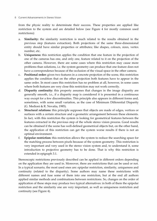
from the physic reality to determinate their success. These properties are applied like restriction to the system and are detailed below (see Figure 4 for mostly common used restrictions):
a. Similarity: the similarity restriction is much related to the results obtained in the previous step (features extraction). Both projections of the same three-dimensional entity should have similar properties or attributes; like shapes, colours, sizes, vertex number, etc.
b. Uniqueness: this restriction applies the condition that one feature in the projection of one of the cameras has one, and only one, feature related to it on the projection of the other camera. However, there are some cases where this restriction may cause more problems than solutions, i.e. the system geometry can produce that one feature does not have a correspondence because of the occlusion of the visual space in the other camera.
c. Positional order: given two features in a concrete projection of the scene, this restriction applies the condition that on the other projection both features have to appear in the same order. In most cases this restriction has no problem at all, however, in some cases where both features are very close this restriction may not work correctly.
d. Disparity continuity: this property assumes that changes in the image disparity are generally smooth, i.e., if a disparity map is considered it is presented in a continuous way except for a few discontinuities. This principle also appears in different forms and, sometimes, with some small variation, as the case of Minimum Differential Disparity (G. Medioni & R. Nevatia, 1985).
e. Structural relations: this principle supposes that objects are made of edges, vertices or surfaces with a certain structure and a geometric arrangement between these elements. In fact, with this restriction the system is looking for geometrical features between the features extracted in the previous step of the whole stereo vision process. Good results can be obtained if the scene has well-defined geometrical objects but, on the other hand, the application of this restriction can get the system worse results if there is not an optimal environment.
f. Epipolar restriction: this restriction allows the system to reduce the searching space for the matching process between pixels because of the system geometry. This restriction is very important and very used in the stereo vision system and, to understand it, some introduction to projective geometry has to be done. That is why this restriction is extended in epigraph 3.1.
Stereoscopic restrictions previously described can be applied in different orders depending on the application they are used in. Moreover, there are restrictions that can be used or not. In a typical scenario, the most used ones are: epipolar restriction, similarity, uniqueness and continuity (related to the disparity). Some authors may name these restrictions with different names and fuse some of them into one restriction, but at the end all authors applied similar methods and combinations between restrictions. So, changes on the order of application of these steps may produce two typical alternatives: in both of them the epipolar restriction and the similarity one are very important, as well as uniqueness restriction and continuity (see Figure 4).

Stereo Matching: From the Basis to Neuromorphic Engineering 7
Figure 4. Restrictions application order in the matching process.
3.1. Epipolar restriction
The epipolar geometry is the intrinsic projective geometry between two views. The application of projective geometry techniques in computer vision is most notable in the Stereo Vision problem which is very closely related to Structure-from-Motion. Unlike general motion, stereo vision assumes that there are only two shots of the scene. In principle, then, one could apply stereo vision algorithms to a structure from motion task.
Applying projective geometry to stereo vision is not new and can be traced back from 19th century photogrammetry to work in the late sixties by Thompson (E. Thompson, 1968). However, interest in the subject was recently rekindled in the computer vision community thanks to important works in projective invariants and reconstruction by Faugeras (O. Faugeras, 1992) and Hartley (R. Hartley, R. Gupta, & T. Chang, 1992).
Epipolar restriction is independent of scene structure, and only depends on the cameras' internal parameters and relative pose. The epipolar geometry between two views is essentially the geometry of the intersection of the image planes with the pencil of planes having the baseline as axis (the baseline is the line joining the camera centres). This geometry is usually motivated by considering the search for corresponding points in stereo matching, and this explanation will start from that objective here.
Figure 5. Epipolar restriction.

Current Advancements in Stereo Vision 8
Suppose that a point X in a third-dimensional space is imaged in two views (see Figure 5), at x in the first, and x’ in the second one. The relation between both points is inherent to the scene and can be seen in Figure 5. As shown in the image: points x and x’, space point X, and camera centres are coplanar (denote this plane as ). Clearly, the rays back-projected from x and x’ intersect at X, and the rays are coplanar, lying in . This latter property is the one that is of most significance in searching for a correspondence.
Suppose now that x is the only known point, it can be determined how the corresponding point x’ is constrained. The plane is determined by the baseline and the ray determined by x. From above it is known that the ray corresponding to the (unknown) point x’ lies in , hence the point x’ lies on the line of intersection l’ of with the second image plane. This line l’ is the image in the second view of the ray back-projected from x. In terms of a stereo correspondence algorithm the benefit is that the search for the point corresponding to x need not cover the entire image plane but can be restricted to the line l’. These lines are known as epipolar lines. So the matching problem is reduced to seek for the corresponding point; not in the whole image, but only in those points lying on the epipolar line of the other camera.
The linear epipolar geometry formulation also exhibits sensitivity to noise (i.e. in the 2D image measurements) when compared to nonlinear modelling approaches. One reason is that each point can be corresponded to any point along the epipolar line in the other image. Thus, the noise properties in the image are not isotropic with noise along the epipolar line remaining completely unpenalized. Thus, solutions tend to produce high residual errors along the epipolar lines and poor reconstruction. Experimental verification of this can be found in the references (A.J. Azarbayejani, 1997).
After the epipolar restriction has been detailed, this work will continue with the general matching problem. Next, before the discussion of the matching process problems and the application to Neuromorphic Engineering, a global classification of the matching algorithms will be shown.
3.2. Matching algorithms classification
From the previous explanations about matching process, it can be resumed that the projection for a three-dimensional-space point is determined for each image of the stereo pair during the image matching. The solution for the matching problem demands to impose some restrictions on the geometric model of the cameras and the photometric model of the scene objects. Of course, this solution implies a high computational cost.
A common practice is trying to relate the pixel of an image with its counterpart on the other one. Some authors divide the matching methods depending on the restrictions that exploits. According to this, a high-level division could be as follows:
a. Local methods: Methods that applies restrictions on a small number of pixels around the pixel under study. They are usually very efficient but sensitive to local ambiguities of the regions (i.e. regions of occlusion or regions with uniform texture). Within this

Stereo Matching: From the Basis to Neuromorphic Engineering 9
group are: the area-based method, features-based method, as well as those based on gradient optimization (S.B. Pollard, 1985).
b. Global methods: Methods that applies restrictions on the entire image itself. They are usually less sensitive to local peculiarities and they add support to some regions that are difficult to study in a local way. However, they tend to be computationally expensive. Within this group are the dynamic programming methods and nearest neighbour methods (M. Bleyer & M. Gelautz, 2004).
Each technique has its advantages and disadvantages and these ones depends on the system restrictions and the cameras geometry (G. Pajares et al, 2006), as said before. The best matching method would be one that applies the advantages of each of the methods explained before; this is a method that processes the given information using local and global methods and, after it, compares both results and combines them to obtain better results than both of them separately. This fact is very difficult to obtain because the system would need huge computational resources and would not work in a real time system.
Local methods will be discussed later in more detail because they are the most used ones. This work won’t go further into global methods because they are rarely used due to their high computational cost.
3.2.1. Area-based matching algorithms
Area-based techniques to solve matching problems in a typical stereo vision system use intensity patterns in the neighbourhood of a concrete pixel to determinate its correlation. It is calculated the correlation between the distribution of disparity for each pixel in an image using a window centred at this pixel, and a window of the same size centred on the pixel to be analysed in the other image (see Figure 6). The problem is to find the point to be adjusted properly at first.
The effectiveness of these methods depends largely on the width of the taken window. Thus, it can be assumed that the larger the window, the better the outcome. However, the computing power requirements increase in these methods as the window becomes bigger. The biggest problem in these methods is to find a window size large enough to ensure finding a correspondence (S.B. Pollard, 1985) between two images in most of the cases, but the window width should not be overwhelmed as it would cause a huge latency in our system. Also, if the window size is close to the total size, it would be deriving to the global methods, which were not taken into account because of their computational inefficiency.
The main advantage of these correlation mechanisms has been previously named in multiple times and it is very easy to deduce it: the computational efficiency (T. Tuytelaars et al., 2000). This characteristic is crucial if the resulting system is wanted to be performed fairly well in real time. On the other hand, the main drawbacks in digital systems primarily focus on results:
Working directly with each pixel: it can be observed a high sensitivity to distortions due to the change of point of view, as well as contrast and illumination changes.

Current Advancements in Stereo Vision 10
The presence of edges in the windows of correlation leads to false matches, since the surfaces are intermittent or in a hidden image has an edge over another.
Are closely tied to the epipolar constraints (D. Papadimitriou & T. Dennis, 1996).
Figure 6. Window correlation.
Therefore, area-based stereo vision techniques look for cross correlation intensity patterns in the local vicinity or neighbourhood of a pixel in an image (L. Tang, C. Wu & Z. Chen, 2002; B. McKinnon & J. Baltes, 2004), with intensity patterns in the same neighbourhood for a pixel of another image. Thus, area-based techniques use the intensity of the pixels as an essential characteristic.
3.2.2. Features-based matching algorithms
As opposed to area-based techniques, the features-based techniques need an image pre-processing before the image matching process (see Figure 7). This pre-processing consists of a feature extraction stage from both images, resulting in the identification of features of each image. In turn, some attributes have to be extracted to be used in the matching process. Thus, this step is closely linked to the matching stage in those matching algorithms based on features because, without this step, the algorithm would not be able to have enough information to make inferences and obtain the image correlation.
Figure 7. Area-based and features-based algorithms

Stereo Matching: From the Basis to Neuromorphic Engineering 11
For features-based stereo vision, symbolic representations are taken from the intensity images instead of directly using the intensities. The most widely used features are: breakpoints isolated chains of edge points or regions defined by borders. The three above features make use of the edge points. It follows that the end points used as primitives are very important in any stereo-vision process and, consequently, it is common to extract the edge points of images. Once the relevant points of edge have been extracted (see Figure 8), some methods use arrays of edge points to represent straight segments, not straight segments, closed geometric structures which form geometric structures defined or unknown.
Figure 8. Edge detections in a features-based algorithm.
Aside from the edges, the regions are another primitive that can be used in the stereo-vision process. A region is an image area that is typically associated with a given surface in the 3D scene and is bounded by edges.
With the amount of features and depending on the matching method that will be used, an additional segmentation step may be necessary. In this step, additional information would be extracted from the known features. This information is calculated based on inferences from the known characteristics. Thus, the matching algorithm that receives the inferred data possesses much more information than the algorithm that works directly on the pixel intensity.
Once the algorithm has both vectors with the inferred features from the two images, it searches in the vectors looking for similar features. The matching algorithm is limited to a search algorithm on two features sets. So, it is understandable to say that the bulk of computation corresponds to the feature extraction algorithm and the inference process. This fact will affect to the system it is going to be located in (in a real-time system with a low power consumption it is difficult to use this kind of algorithm). The main advantages of these techniques are:
Better stability in contrast and illumination changes. Allow comparisons between attributes or properties of the features. Faster than area-based methods since there are fewer points (features) to consider,
although require pre-processing time. More accurate correspondence since the edges can be located with greater accuracy.

Current Advancements in Stereo Vision 12
Less sensitive to photometric variations as they represent geometric properties of the scene.
Focus their interest on the scene that has most of the information.
Despite these advantages, features-based techniques have two main drawbacks, which are easily deduced from the characteristics described above. The first drawback is the high degree of dependence on the chosen primitives of these techniques. This can lead to low quality or unreliable results if the chosen primitives are not successful or are not appropriate for these types of images. For example, in a scene with few and poorly-defined edges, delimiters would not be advisable to select regions as primitive.
Another drawback is derived from the characteristics of the pre-processing stage. Previously, this step was described as a feature extraction mechanism of the two images and the inference or properties of the highest level in each of them. As stated above, there is a high computational cost associated to this pre-processing stage, to the point that using digital cameras with existing high-level algorithms running on powerful machines cannot match the real time processing.
However, in general purpose equipment, this technique is the most commonly used because of its results. In classic machine vision, this research branch has been the most deepened in (P. J. Herrera et al, 2009; D. Scaramuzza et al, 2008, P. Premaratne & F. Safaei, 2008).
With these explanations, a global perspective to matching algorithms has been presented as well as classified in different types. All of them have been exposed and evaluated with their advantages and drawbacks. Next, this work introduce the reader to the concept of Neuromorphic Engineering and, after that, a stereo matching approximation to a neuromorphic system is shown.
4. Neuromorphic engineering
Throughout history, many times engineers have achieved solutions to very difficult problems inspired by nature behavior to solve them. This has been applied in many diverse fields, so it is very common to find these bio-inspired systems in the near environment. This is the origin of Neuromorphic Engineering.
However, there are too much unsolved problems in nature that, maybe, could be solved using this kind of mechanisms applied directly to the problems themselves. In neuromorphic engineering, researchers look for the human being “controller” or, what is the same, the nervous system; trying to mimic it, using inverse engineering (V. Chan et al, 2007; Shih-Chii Liu et al, 2010). These systems obtained after looking for answers in the nervous system are called neuro-inspired systems (M. Domínguez-Morales et al, 2011). They are a subset of the bio-inspired systems that try to solve common engineer problems using systems based on the manner that nervous system codifies and processes the information. This is a continuous evolving research branch thanks to the work of many neuromorphic engineers.
Stereo Matching: From the Basis to Neuromorphic Engineering 13
Focusing on the vision problems, digital vision systems process sequences of frames from conventional frame-based video sources, like cameras (as was shown in previous epigraphs). For performing complex object recognition algorithms, sequences of computational operations must be performed for each frame (this is like the processing chain in stereo vision that was shown previously). The required computational power and speed required make it difficult to develop a real-time autonomous system. However brains perform powerful and fast vision processing using millions of small and slow cells working in parallel in a totally different way. Primate brains are structured in layers of neurons, in which the neurons in a layer connect to a very large number (~104) of neurons in the following layer (G. M. Shepherd, 1990). Many times the connectivity includes paths between non-consecutive layers, and even feedback connections are present.
Vision sensing and object recognition in brains are not processed frame by frame; they are processed in a continuous way, spike by spike (a spike is like an electronic pulse produced in the brain by neurons), in the brain-cortex. The visual cortex is composed by a set of layers (G. M. Shepherd, 1990), starting from the retina. The processing starts when the retina captures the information. In recent years significant progress has been made in the study of the processing by the visual cortex. Many artificial systems that implement bio-inspired software models use biological-like processing that outperform more conventionally engineered machines (J. Lee, 1981; T. Crimmins, 1985; A. Linares-Barranco, 2010). However, these systems generally run at extremely low speeds because the models are implemented as software programs. For real-time solutions direct hardware implementations of these models are required. A growing number of research groups around the world are implementing these computational principles onto real-time spiking hardware through the development and exploitation of the so-called AER (Address Event Representation) technology.
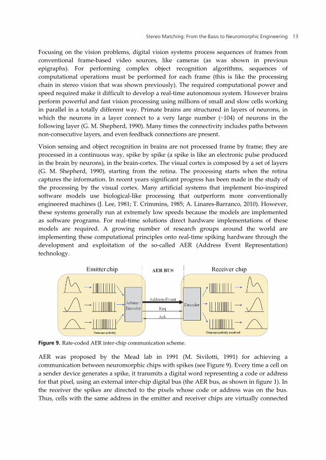
Figure 9. Rate-coded AER inter-chip communication scheme.
AER was proposed by the Mead lab in 1991 (M. Sivilotti, 1991) for achieving a communication between neuromorphic chips with spikes (see Figure 9). Every time a cell on a sender device generates a spike, it transmits a digital word representing a code or address for that pixel, using an external inter-chip digital bus (the AER bus, as shown in figure 1). In the receiver the spikes are directed to the pixels whose code or address was on the bus. Thus, cells with the same address in the emitter and receiver chips are virtually connected

Current Advancements in Stereo Vision 14
by streams of spikes. Arbitration circuits ensure that cells do not access the bus simultaneously. Usually, AER circuits are built with self-timed asynchronous logic.
Several works are already present in the literature regarding spike-based visual processing filters. Serrano et al. presented a chip-processor able to implement image convolution filters based on spikes that work at very high performance parameters (~3GOPS for 32x32 kernel size) compared to traditional digital frame-based convolution processors (B. Cope, 2006; B. Cope, 2005; A. Linares-Barranco, 2010).
There is a community of AER protocol users for bio-inspired applications in vision and audition systems, as evidenced by the success in the last years of the AER group at the Neuromorphic Engineering Workshop series. One of the goals of this community is to build large multi-chip and multi-layer hierarchically structured systems capable of performing complicated array data processing in real time. The power of these systems can be used in computer based systems under co-processing.
5. Stereo matching in AER system
Hitherto, the reader has had the possibility of getting into the state of the art in stereo vision systems, as well as learning about bio-inspired systems. In this epigraph, a stereo matching algorithm for an AER system will be explained.
First, it is very important to know what type of bio-inspired camera (retina) is going to be used. In this work, and many others done in the same research group, a couple of DVS128 retinas are used (P. Lichtsteiner, C. Posh & T. Delbruck, 2008). This kind of retina has a resolution of 128 rows plus 128 columns, so it has 16384 pixels. The importance of this retina is not the resolution itself, but the work behaviour. These retinas implement the brightness derivative in time, so they only see changes in luminosity or, after a simplification, objects in movement. The mechanism of transmitting the information is centred on a couple of arbitrators (one for the row and the other for the column) and sent via a parallel bus using seven lines for the row (27 = 128) and another seven for the column.
However, there is no transmission about intensity of the pixel itself. This information is codified in time using the pulses frequency: this is the pulse frequency modulation (PFM). So there are two different possibilities when trying to emulate classical machine vision algorithms behaviour using these retinas: first one is implementing some kind of spiking algebra (A. Jimenez-Fernandez, 2010; A. Jimenez-Fernandez et al, 2012) to attach the problem and solve it in a different way, this option is an important branch of research currently in development and some excellent results have been obtained using it; the second one is trying to adapt classical algorithms to the new paradigm in some way. The final step of this work evaluates similarities between classical stereo vision matching algorithms and AER retinas obtained data, to obtain a first-approach matching algorithm in an AER stereo vision system, full-working on programmable hardware (VHDL over a FPGA).
As a first approximation, it could be considered making an adaptation of the features-based algorithms to obtain a consistent algorithm with good results (see epigraph 3.2.2). However,

Stereo Matching: From the Basis to Neuromorphic Engineering 15
in this case there is lots of efficiency problems mainly derived from the early stages of pre-processing and inference used to obtain the full set of features from each frame and the second-level features obtained by inference. In order to define an algorithm that is feasible in an AER stereo vision system it has to be taken into account its properties and the goals that the system is wanted to achieve.
At epigraph four it was mentioned an introduction about neuromorphic engineering and, deeper, a first look to AER systems, its motivations, current development and research lines related to them. The main goal in this work and in everyone related to bio-inspired systems is to design and build an autonomous and independent system that works in a real-time ambit, with no need to use a computer to run high-level algorithms. The efficiency of the system does not have to be as important as real-time processing; due to the nature of AER systems, it is not important to make some error in calculations, because its processing is applied in a continuous way and it will be automatically self-corrected over time. Although quality is sacrificed in the results, it cannot be afforded to perform a pre-processing and inference stages, which slow down the full system making impossible to obtain a real-time processing. Moreover, due to the independence requirement derived from the AER system, sending information to a computer via a typical serial port can alter timing constraints of these systems and make it difficult to correlate pixels from both retinas, unless some kind of timestamp is transmitted with each spike. This fact will increase the bandwidth used and can make the computer to lose information. Another major setback to consider in this case is that information transmitted by AER system is closely linked to time and to the number of spikes received and, in serial communication, information is sent in packets and it may have a large time span without receiving any spike.
Resuming, the information in an AER system is a continuous flow that cannot be stopped: the information can only be processed or discarded; each spike is transmitted by a number of communication lines, and contains information from a single pixel. Moreover, the intensity of a pixel dimension is encoded in the spike frequency received from that particular pixel. The AER retinas used by research groups are up to a 128x128 resolution (nowadays some groups work with a 320x240 resolution retina), which means that measure brightness changes over time. Thus, taking a load of 10% in the intensity of the pixels, it would be in the range of more than four hundred thousand pulses to describe the current state of the scene with a single retina. This is too much information to be pre-processed. Furthermore, the stereo system has two retinas (double data rate), so the information transmission is a critical point to be taken into account.
This system is required to be independent and based on an FPGA connected to the outputs of two AER retinas (see Figure 10). The FPGA will process the information using the concrete algorithm and transmits the resulting information using a parallel AER bus to an USBAERmini2 PCB (R. Berner et al, 2007), which is used like a monitor between the output of the system and the computer. This is responsible for monitoring AER traffic received and transmitted by USB from and to a computer. Should be noted that the computer is only used to verify that the concrete algorithm running on the FPGA works as required; the computer itself is not used to process any information.

Current Advancements in Stereo Vision 16
Taking into account the digital algorithms, the second option is to use a variant of the area-based matching algorithms (T. Tuytelaars, 2000). In this case, the topic to consider would be the results because, as discussed above, these algorithms do not require pre-processing but not ensure result reliability.
Among the problems related to the area-based matching algorithms, AER retinas include failures caused by variations in the brightness and contrast. This involved the properties of AER retinas used, which do not show all the visual information it covers, but the information they send is the spatial derivative in time. This means that it is only appreciated the information of moving objects, while the rest of non-mobile environment is not "seen". In addition, these retinas have very peculiar characteristics related to information processing. These characteristics make them immune to variations in brightness and contrast (lightness and darkness does not interfere with transmitted information). With this retina property managed to avoid the major drawback of area-based algorithms. The next proposed algorithm is linked to the information received from the AER bus. It also inherits similar properties from area-based algorithms, but adapted to the received information. It is proposed an algorithm able to run in a standalone environment in a FPGA, which receives traffic from two AER retinas through a parallel bus.
The algorithm itself work as this: at a first step, it counts the received spikes for each pixel of the image and store this information in a table. So that, this table has pixel intensity measures derived from the moving objects detected by each retina at every moment. The algorithm will mainly find correspondences between the two tables of spike counters. If the reader has paid attention to what explained in the rest of the chapter, it may be noticed that in practice what is being done is a process of digitalization of the bio-inspired system. In fact, at this point the algorithm is performing integration over time of the information received from each retina. So, the stored tables are really two frames, each one corresponding to one different retina. Given that, there are two problems involving the algorithm and the properties of AER retinas.
A major issue about the retinas is their unique properties (AER output frequency, firing intensity threshold of the pixels, etc) of each retina and its pre-configuration setting. Thus, the information of the same pixel in both retinas does not have to be sent at the same time and there could be a frequency variation between both of them; furthermore, both retinas are not presented in a parallel way, so they are put in a concrete angle. To prevent this, it is proposed a fuzzy matching algorithm based on spikes frequency. First, the hardware system will be shown.
Figure 10. Complete system with all the elements used

Stereo Matching: From the Basis to Neuromorphic Engineering 17
All the elements that compose the system are these (from left to right, see Figure 10): two DVS128 retinas (P. Lichtsteiner, C. Posh & T. Delbruck, 2008), two USB-AER, a Virtex-5 FPGA board (AVNET reference), an USBAERmini2 (R. Berner et al, 2007) and a computer to watch the results with jAER software (jAER reference). Next, the non-explained components in this system will be talked about them.
USB-AER (see Figure 11, left) board was developed in the Robotic and Computer Technology Lab during the CAVIAR project (R. Serrano-Gotarredona et al, 2009), and it is based on a Spartan II FPGA with two megabytes of external RAM and a cygnal 8051 microcontroller. To communicate with the external world, it has two parallel AER ports (IDE connector). One of them is used as input, and the other is the output of this board. In the whole system two USB-AER boards have been used, one for each retina. In these boards it has been synthetized in VHDL a filter called Background-Activity-Filter, which allows the system to eliminate noise from the stream of spikes produced by each retina. This noise (or spurious) is due to the nature of analog chips and since anything can be done to avoid it in the retina, it has been filtered in some way. So, at the output of the USB-AER boards, there is the same information given by the retinas but filtered (better quality information).
The other board used is a Xilinx Virtex-5 board, developed by AVNET (AVNET reference). This board is based on a Virtex-5 FPGA and mainly has a big port composed of more than eighty GPIOs (General Purpose Inputs/Outputs ports). Using this port, it has been connected an expansion/testing board, which has standard pins, and it has been used to connect two AER inputs and one output to it.
Figure 11. Left, USB-AER board; right, Virtex-5 FPGA board.
The Virtex-5 (see Figure 11, right) implements the whole processing program, which works with the spikes coming from each retina, processes them and obtains the final results. The system behaviour and its functionality are shown in the following sections.
The fuzzy algorithm proposed works as explained next. It will not seek exactly the same levels of intensity in both virtual frames, but would admit an error in the range of 5 and 8% of these levels (in the proposed case, with 256 intensity levels, that means that it is admitted a range of 12-20 levels error). The exact parameters used for the final results depend on the environment where the matching process is applied: if it is an open space it needs a bigger

Current Advancements in Stereo Vision 18
error range, but if it is used a laboratory environment, there is no need for a big error range. This parameter can be adjusted modifying the VHDL code.
The first problem is solved, but it is almost very inefficient algorithm if a pixel by pixel correlation is used. To solve it, the principles of area-based matching algorithms are used in this algorithm. The system is not limited to one pixel correspondence search, neither a global search of the pixel; each correspondence is looked for over a window of a concrete width in the other virtual frame. This window is centred in the position given by the original pixel of the first retina. The size of the window used by the algorithm depends on the environment too, but also in the system calibration. In the system proposed, both retinas are allocated at a distance of 13’5 centimetres between them and in an angle of 86’14 degrees to obtain a focal collision of one meter. To emphasize, the correspondence between each pair of pixels from both retinas will be done separately using the fuzzy matching algorithm explained above (G.Pajares, 2006). In fact, the system divides the correspondence map into regions and each process looks for a correspondence over its region alone. This full process can only be done because of the VHDL implementation over an FPGA, which allows a massive parallel multiprocessing execution (depending on the number of logic cells allocated in the FPGA) (A. Jimenez-Fernandez et al, 2010-2).
The system functionality has been presented, but there is an important element that has not been talk about yet. This element is in charge of controlling the virtual frames timing. In fact, in a classical machine vision system is easy to understand that a video is sent using frames and, each frame, contains the information of the entire scene in a concrete instant. Furthermore, these frames are transmitted using a concrete period (called fps or frames per second). Returning to the system described in this work (see Figure 12), artificial frames have been created but the information stored in them in the integration of the information during all the time, there is no timestamp that divides one virtual frame from the next. That is why the system needs a daemon that preserves this harmony. This daemon will be considered a process in charge of reset all the spikes counters time to time to avoid counters overflow.
Figure 12. Virtex-5 with AER retinas and USBAERmini2.

Stereo Matching: From the Basis to Neuromorphic Engineering 19
There are many adjustable parameters on this system depending on the environment where the stereo vision matching is applied and on the area it is going to be used. The whole system is under testing stages: first it was submitted to simulation tests over Matlab software and, at the present, the system is under testing directly on the FPGA.
6. Conclusions
Humanity has experienced great changes in the field of vision, but they have always been aimed to get the results of the vision system of a human being.
In this work, an introduction to stereo vision systems has been shown, as well as an explanation about all the typical steps used in a common stereo vision system. It has entered deeply into the most important stage: the matching process, which has been theoretically analysed in depth, showing and explaining most typical algorithms that solve this problem in classic machine vision.
Next, a relatively new processing and encoding paradigm has been explained with its advantages and drawbacks. It has been discussed the existing relations between classical stereo matching process and the stereo matching process related to this new paradigm (AER stereo matching process).
Finally, an Address-Event-Representation stereo matching algorithm has been detailed using classical stereo vision concepts and adapting them to the bio-inspired system. As well, the AER stereo system has been shown and all the elements that compose it have been exposed.
Author details
M. Domínguez-Morales, A. Jiménez-Fernández, R. Paz-Vicente, A. Linares-Barranco and G. Jiménez-Moreno Robotic and Computer Technology Group - University of Seville, Spain
Acknowledgement
This work has been supported by the Spanish Science and Education Ministry Research Projects TEC2009-10639-C04-02 (VULCANO).
7. References
A. Rosenfeld (1969). First Textbook in Computer Vision: Picture Processing by Computer, Academic Press, New York.
C. Dyer. (2001). Volumetric scene reconstruction from multiple views, In L.S. Davis, editor, Foundations of image analysis. Kluwer, Boston.
J.Weng, P. Cohen, & M. Herniou (1992). Camera Calibration with Distortion Models and Accuracy Evaluation, IEEE Trans. Patt. Anal. Machine Intell., vol. 14, no. 10, pp. 965–980.

Current Advancements in Stereo Vision 20
Qurban Memon & Sohaib Khan (2001). Camera Calibration and Three-Dimensional World Reconstruction of Stereo-Vision Using Neural Networks, International Journal of Systems Science.
R. Tsai (1987). A versatile camera calibration technique for high-accuracy 3D machine vision metrology using off-the-shelf TV cameras and lenses, IEEE Transactions on Robotics and Automation.
J. Douret & R. Benosman (2004). A multi-cameras 3D volumetric method for outdoor scenes: a road traffic monitoring application, International Conference on Pattern Recognition (ICPR).
A. Rosenfeld & А. С. Как (1982). Digital Picture Processing, Academic Press, New York, 1976; 2nd ed. (2 vols.).
S. T. Barnard & M. A. Fischler (1982). Computational Stereo, Journal ACM Computing Surveys (CSUR), vol. 14 Issue 4.
R. Benosman & J. Devars (1998). Panoramic stereo vision sensor, International Conference on Pattern Recognition.
M. Dominguez-Morales et al (2011). Image Matching Algorithms using Address-Event-Representation, International Conference on Signal Processing and Multimedia Applications (SIGMAP).
G. Medioni & R. Nevatia (1985). Segment Based Stereo Matching, Computer Vision, Graphics and Image Processing, 31, 2-18.
E. Thompson (1968). The projective theory of relative orientation, Photogrammetria, no. 23(1): 67-75.
O. Faugeras (1992). What can be seen in three dimensions from an uncalibrated stereo rig?, Proceedings of the 2nd European Conference on Computer Vision, pages 563-578, Santa Margherita Ligure, Springer-Verlag.
R. Hartley, R. Gupta, & T. Chang (1992). Stereo from uncalibrated cameras, Proceedings of the Conference on Computer Vision and Pattern Recognition, pages 761-764, Urbana-Champaign.
A. J. Azarbayejani (1997). Nonlinear Probabilistic Estimation of 3-D Geometry from Images, PhD thesis, Massachusetts Institute of Technology.
S. B. Pollard et al (1985). PMF: A stereo correspondence algorithm using a disparity gradient limit, Perception, 14:449-470.
M. Bleyer & M. Gelautz (2004). A Layered Stereo Algorithm Using Image Segmentation and Global Visibility Constraints, ICIP, pp. 2997-3000.
G. Pajares et al (2006). Fuzzy Cognitive Maps for stereovision matching, Pattern Recognition, 39, 2101-2114.
T. Tuytelaars et al (2000). Wide baseline stereo matching based on local, affinely invariant regions, British Machine Vision Conference (BMVC).
D. Papadimitriou & T. Dennis (1996). Epipolar line estimation and rectification for stereo image pairs, IEEE Transactions on Image Processing, 5(4):672-676.
L. Tang, C. Wu & Z. Chen (2002). Image dense matching based on region growth with adaptive window, Pattern Recognition Letters, 23, 1169–1178.

Stereo Matching: From the Basis to Neuromorphic Engineering 21
B. McKinnon & J. Baltes (2004). Practical region-based matching for stereo vision, proceedings of 10th International Workshop on Combinatinal Image Analysis (IWCIA), Springer, pp. 726–738, LNCS 3322.
P. J. Herrera et al. (2009). A Featured-Based Strategy for Stereovision Matching in Sensors with Fish-Eye Lenses for Forest Environments, Sensors, 9, 9468-9492
D. Scaramuzza, N. Criblez, A. Martinelli, R. Siegwart (2008). Robust feature extraction and matching for omnidirectional images, Field and Service Robotics, Springer, vol. 42, pp. 71–81.
P. Premaratne & F. Safaei (2008). Feature based Stereo correspondence using Moment Invariant, proceedings of the 4th International Conference on Information and Automation for Sustainability (ICIAFS), pp. 104–108.
G. M. Shepherd (1990). The Synaptic Organization of the Brain, Oxford University Press, 3rd Edition.
Vincent Chan, Shih-Chii Liu & A. van Shaik (2007). AER EAR : A Matched Silicon Cochlea Pair with Address Event Representation Interface, IEEE Transactions on Circuits and Systems, 54, 48-59.
Shih-Chii Liu et al (2010). Event-based 64-channel binaural silicon cochlea with Q enhancement mechanisms, proceedings of IEEE International Symposium on Circuits and Systems (ISCAS), pp. 2027-2030.
M. Dominguez-Morales et al. (2011). An approach to distance estimation with stereo vision using Address-Event-Representation, International Conference on Neural Information Processing (ICONIP).
J. Lee (1981). A Simple Speckle Smoothing Algorithm for Synthetic Aperture Radar Images, Man and Cybernetics, vol. 13.
T. Crimmins (1985). Geometric Filter for Speckle Reduction, Applied Optics, vol. 24, pp. 1438-1443.
A. Linares-Barranco et al. (2010). AER Convolution Processors for FPGA, International Symposium of Circuits And Systems (ISCAS).
M. Sivilotti (1991). Wiring Considerations in analog VLSI Systems with Application to Field-Programmable Networks, Ph.D. Thesis, Caltech.
B. Cope et al. (2005). Have GPUs made FPGAs redundant in the field of video processing?, International Conference on Field-Programmable Technology (FPT).
B. Cope et al (2006). Implementation of 2D Convolution on FPGA, GPU and CPU, Imperial College Report.
P. Lichtsteiner, C. Posh & T. Delbruck (2008). A 128×128 120dB 15 us Asynchronous Temporal Contrast Vision Sensor, IEEE Journal on Solid-State Circuits, vol. 43, no 2, pp. 566-576.
A. Jiménez-Fernandez (2010). Diseño y evaluación de sistemas de control y procesamiento de señales basados en modelos neuronales pulsantes, Ph.D. Thesis, University of Seville (Spain).
A. Jiménez-Fernandez et al. (2012). A Neuro-Inspired Spike-Based PID Motor Controller for Multi-Motor Robot with Low Cost FPGA, Sensors, vol. 12, no 4, pp. 3831-3856.
R. Berner, T. Delbruck, A. Civit-Balcells & A. Linares-Barranco (2007). A 5 Meps $100 USB2.0 Address-Event Monitor-Sequencer Interface, International Symposium of Circuits And Systems (ISCAS).

Current Advancements in Stereo Vision 22
R. Serrano-Gotarredona et al (2009). CAVIAR: A 45k-Neuron, 5M-Synapse, 12G-connects/sec AER Hardware Sensory-Processing-Learning-Actuating System for High Speed Visual Object Recognition and Tracking, IEEE Transactions on Neural Networks, vol. 20, no. 9, pp. 1417-1438.
T. Tuytelaars et al. (2000). Wide baseline stereo matching based on local, affinely invariant regions, British Machine Vision Conference (BMVC).
A. Jiménez-Fernandez et al (2010-2). Building Blocks for Spike-based Signal Processing, IEEE International Joint Conference on Neural Networks (IJCNN).
AVNET Virtex-5 FPGA board: http://www.em.avnet.com/drc jAER software: http://sourceforge.net/apps/trac/jaer/wiki

Chapter 0
Stereo Vision and Scene Segmentation
Carlo Dal Mutto, Fabio Dominio, Pietro Zanuttighand Stefano Mattoccia
Additional information is available at the end of the chapter
http://dx.doi.org/10.5772/45903
1. Introduction
Scene segmentation is the well-known task of identifying the image regions correspondingto the different scene elements or segments Sk, k = 1, 2..., N belonging to a predefined set Spartitioning the scene in N subsets, each one corresponding to a scene object or to a regionof interest. Beside being an important problem by itself, segmentation is also employed asa preliminary step in many other computer vision tasks, e.g. object recognition or stereovision. A closely related problem, very relevant for the television and movie industries, isvideo-matting which consists in separating the background from the foreground.
Classical segmentation techniques are based on different insights but all of them face theproblem starting from the color information extracted from a single image of the framed scene.Despite the huge efforts put in research, scene segmentation from a single image is an ill-posedproblem still lacking of robust solutions. The intrinsic limit of the classical approaches is thatthe color information contained in an image does not always suffice to completely understandthe scene composition. An example of this limit is depicted in Figure 1(b). Note how the babyand part of the world map on background were associated to the same segment by a classicalsegmentation algorithm based on color only information, due to the very similar colors of thebaby’s skin and of some map regions.
Depth information can also be used for segmentation purposes. In this way some limits ofcolor information based segmentation can be overcome but with side-effect of introducingother problems in regions that have similar depth but different colors. Figure 1(c) reports anexample of this, as the book and the baby’s feet were associated to the same segment dueto their similar depth. The usage of geometry only allows good segmentation performancebut is not always effective. For example it can not solve situations where there are objectsof different colors placed close one to the other, such as two people wearing different clothesbut very close each other, or slanted surfaces crossing multiple depths. At the same timecolor information only can not distinguish objects with similar colors regardless their relativedistance.
Chapter 2

2 Will-be-set-by-IN-TECH
(a) Color image (b) Segmentation on the basis ofcolor data
(c) Segmentation on the basis ofgeometry data
Figure 1. Results of a classical scene segmentation method applied to color or geometry informationonly. Occlusions or pixels discarded by segmentation algorithm are reported in black.
Clearly from Figures 1(b) and 1(c), segmentation based on either color or geometryinformation is likely to fail, since most of the framed scenes contain objects sharing similarcolors or neighbors in the 3D space.
By considering both color and geometry cues in segmentation it is possible to avoid theambiguities described above, as pixels with similar color but distant in 3D space or vice-versaare no longer likely to be mapped to neighboring feature vectors in feature space. It is alsotrue that often the joint usage of color and geometry information as segmentation clues maybe enough for this task. For example, if the algorithm of Figures 1(b) and 1(c) exploited bothcolor and geometry, it would have “realized” that the baby’s feet belong to the “baby segment”since they have the same baby’s skin color though they share the same depth with the book,and that the map regions do not belong to the baby’s segment as well though they share thesame skin color, since they belong to the background and a have a different depth.
Many different approaches exist for the estimation of the 3D scene geometry. They can beroughly divided into active methods, that project some form of light over the scene, likelaser scanners, structured light systems (including the recently released Microsoft’s Kinect)or Time-Of-Flight cameras. Passive methods instead do not use any form of projection andusually rely only on a set of pictures framing the scene. In this class binocular stereo visionsystems are the most common approach due to the simplicity of the setup and to the low cost.The choice of the best suitable system depends upon the trade-off among the system cost,speed and required accuracy.
Stereo vision systems provide estimates of the 3D geometry of a framed scene given two viewsof it, often referred as left and right view respectively. A considerable amount of researchhas been devoted for many years to scene geometry reconstruction by mean of stereo visionmethods, now able to give dense and reliable depth information estimates.
Current literature [15] provides different algorithms to perform this task, each onewith different trade-offs between reconstruction accuracy and efficiency (computational
24 Current Advancements in Stereo Vision

Stereo Vision and Scene Segmentation 3
requirements). Simpler and faster stereo algorithms usually have poor accuracy, especiallyin presence of non-textured regions where the search for the correspondent points in the twoimages is likely to fail. More sophisticated algorithms (e.g. global algorithms), instead, allowin most cases better accuracy at the expense of higher computational costs.
This chapter focuses on how segmentation robustness can be improved by 3D scene geometryprovided by stereo vision systems, as they are simpler and relatively cheaper than mostof current range cameras. In fact, two inexpensive cameras arranged in a rig are oftenenough to obtain good results. Another noteworthy characteristic motivating the choice ofstereo systems is that they both provide 3D geometry and color information of the framedscene without requiring further hardware. Indeed, as it will be seen in following sections,3D geometry extraction from a framed scene by a stereo system, also known as stereoreconstruction, may be eased and improved by scene segmentation since the correspondenceresearch can be restricted within the same segment in the left and right images.
The chapter is organized as follows: Section 2 presents an overall synthesis of the stereovision and clustering methods considered for the proposed scene segmentation framework.The framework is instead illustrated in Section 3. Section 4 provides a comprehensive setof experimental results for scene segmentation of different datasets exploiting the differentcombinations of stereo reconstruction and segmentation algorithms. Section 5 finally drawsthe conclusions.
2. Related works
Current section shortly resumes the state-of-the-art stereo vision and segmentation methodsconsidered in next sections, highlighting their qualities and flaws. Exhaustive surveys ofstereo vision algorithms can be found in [2], [13] and [15]. Recent segmentation techniques arebased on graph theory (e.g. [5]), clustering techniques (e.g. [3, 14]) and many other techniques(e.g. region merging, level sets, watershed transforms and many others). A complete reviewcan be found in [15].
2.1. Stereo vision algorithms
The stereo vision algorithms that have been used inside the proposed framework are herebriefly described.
Fixed Window
The Fixed Window (FW) algorithm is the basic local approach. It aggregates matching costsover a fixed square window and uses, as most local algorithms, a simple winner-takes-all(WTA) strategy for disparity optimization. Similarly to most local approaches, the aggregationof costs within a frontal-parallel support window implicitly assumes that all the points withinthe support have the same disparity. Therefore, FW does not perform well across depthdiscontinuities. Moreover, as most local algorithms, FW performs poorly in texturelessregions. Nevertheless, thanks to incremental calculation schemes [4, 10], FW is very fast.For this reason, despite its notable limitations, this algorithm is widely used in practicalapplications. In the implementation proposed in this chapter, the cost function is the Sumof Absolute Differences (SAD).
25Stereo Vision and Scene Segmentation

4 Will-be-set-by-IN-TECH
Adaptive Weights
The AdaptiveWeights (AW) algorithm [17] is a very accurate local algorithm that uses a fixedsquared window but weights each cost within the support window according to the imagecontent. The weights are first computed, on the left and right image, similarly to a bilateralfilter (i.e. deploying a spatial and a color constraint) and then multiplied to obtain a symmetricweight assigned to each cost within the support window. This method uses the WTA strategyfor disparity optimization and the sum of Truncated Absolute Differences metric for the costs.AW provides very accurate disparity maps and preserves depth discontinuities. However, asfor other local approaches, this method performs poorly in textureless regions. Moreover, thesupport windows shrinks to a few points (or equivalently, AW sets very small weights forseveral points) in presence of highly textured regions making this method error prone. TheAW algorithm is computationally expensive: it requires minutes to process a typical stereopair (the authors report 1 minute for small size images).
Segment Support
The Segment Support (SS) algorithm [16] is a local algorithm that aims at improving theAW approach by explicitly deploying segmentation. Similarly to AW, it aggregates weightedcosts within a square support window of fixed size. Starting from the stereo pairs and thecorresponding segmented stereo pairs, SS computes the weights on each image according tothe following strategy: the weights of the points belonging to the same segment in whichthe central points lies is set to 1. The weight of the points outside such a segment are setaccording to color proximity constraint only and discarding the spatial proximity constraint.The overall weight assigned to each point is computed similarly to AW. In [16] it was shownthat this strategy allows SS to improve the effectiveness of AW near depth discontinuitiesand in presence of repetitive patterns and highly textured regions. However, similarly toother local approaches, this method performs poorly in textureless regions. Although thesegmentation of the stereo pairs can be quickly performed, SS has an execution time higherthan AW. However, in [8] was proposed a block-based strategy referred to as FSD (FastSegmentation-driven), inspired by [9], that enables to obtain equivalent results in a fractionof the time required by SS. It is very interesting to apply SS or FSD in the segmentationframework of Figure 2, because there is a segmentation step both before computing disparityand after the stereo matching calculation. In this work experimental results are reported onlywith SS.
Fast Bilateral
The Fast Bilateral Stereo (FBS) approach [9] combines the effectiveness of the AW approachwith the efficiency of the traditional FW approach enabling results comparable to AW muchmore quickly. In this algorithm the weights are computed on each image and on a blockbasis with respect to the central point according to a strategy similar to AW. The weightassigned to each block is related to the difference between the color intensity of the centralpoint and the average color intensity of the block. The costs within each block are computed,very efficiently, on a point basis by means of incremental calculation schemes. Therefore, ateach point within a block, this method assigns the same weight and its point-wise matchingcost. Disparity optimization is based on the WTA strategy. With block of size 3 × 3, FBSobtain results comparable to AW, well preserving depth discontinuities, in a fraction of the
26 Current Advancements in Stereo Vision

Stereo Vision and Scene Segmentation 5
time required by AW. Increasing the block size decreases the accuracy of the disparity mapsbut reduces the execution time further. Moreover, in [9] it was shown that computing weightson block basis makes this method more robust to noise compared to AW. Similarly to otherlocal algorithms described so far, FBS performs poorly in textureless regions.
Semi-Global Matching
The Semi Global Matching (SGM) algorithm [7] explicitly models the 3D structure of thescene by means of a point-wise matching cost and a smoothness term. However, thismethod is not a traditional global approach since the minimization of the energy functionis computed, similarly to Dynamic Programming or Scanline Optimization approaches, ina 1D domain [13]. That is, several 1D energy functions computed along different pathsare independently and efficiently minimized and their costs summed up. For each point,the disparity corresponding to the minimum aggregated cost is selected. In [7] the authorproposes to use 8 or 16 different independent paths. The SGM approach works well neardepth discontinuities, however, due to its (multiple) 1D disparity optimization strategy,produces less accurate results than more complex 2D disparity optimization approaches.Despite its memory footprint, this method is very fast (it is the fastest among the consideredalgorithms) and potentially capable to deal with poorly textured regions.
Stereo Graph Cut
The Graph Cut stereo vision algorithm (GC) introduced in [1] is a global stereo visionmethod. It explicitly accounts for depth discontinuities by minimizing an energy functionthat combines a point-wise matching cost and a smoothness term. The GC algorithm modelsthe 3D scene geometry with a Markov random field in a Bayesian framework and determinesthe stereo correspondence solving a labeling problem. The energy function is representedas a graph and its minimization is done by means of Graph Cut, an efficient algorithm thatrelies on the Min-Cut/Max-Flow theorem. As most global methods, GC is computationallyexpensive and has a large memory footprint. However, as most global algorithms, it can dealwith depth discontinuities and textureless regions.
2.2. Segmentation methods
Three different clustering schemes have been considered:
Segmentation by k-means clustering
K-means is a classical central grouping clustering algorithm. It is very simple to implementand it is pretty fast. It is not very precise when applied to scene segmentation, because itassumes that the distribution of the considered feature vectors pi representing the pointspi, i = 1, ..., N is a mixture of Gaussians. This assumption is not generally verified in thescene segmentation context and for this reason this clustering method applied to the set Vmay give poor results.
Segmentation by mean-shift
The mean-shift algorithm [3] is a standard non-parametric feature-space analysis techniqueexploitable as a clustering algorithm. It aims at locating the maxima of a density function,
27Stereo Vision and Scene Segmentation

6 Will-be-set-by-IN-TECH
given some samples drawn from the density function itself. It is useful for detecting the modesof a density, and therefore for clustering the feature vectors in a very efficient way. Mean-shiftclustering is very fast, but prone to return outliers. However it is worth considering thisclustering technique since it is very fast, quite reliable and widely used in computer visionand image analysis.
Segmentation by spectral clustering with Nyström method
This method, proposed in [14], is a state-of-the-art clustering algorithm based upon pairwiseaffinity measures computed between all possible couples of points in S . It does not imposeany model or distribution on the points pi, i = 1, ..., N, and therefore its results in practicalsituations are more accurate and robust than those of k-means and mean-shift. Spectralclustering alone is very expensive for both CPU and memory resources. This characteristicis intrinsic to the nature of the algorithm, because the computation of a pairwise affinitymeasure between all the points pi ∈ S requires to build a graph that has a node for eachpoint and an edge between each couple of points. Such graph is usually very large. However,one may obtain an approximated version of such a graph by imposing that not all the pointsare connected. The Nyström method, proposed in [6], is a way to approximate the graph,based on the integral eigenvalue problem. Spectral clustering with Nyström method providesa nice framework to incorporate the fact that S has to be partitioned into subsets where colorand 3D geometry are homogeneous. The resulting speed of spectral clustering with Nyströmmethod is comparable with the ones of k-means and mean-shift.
Table 1 roughly represents the differences in accuracy (final segments) and efficiency (executiontime) among the considered segmentation methods.
Method Accuracy Execution time
K-means Low Fast
Mean-Shift Good Fast
Spectral Clustering High Slow
Spectral clust. with Nyström method High Fast
Table 1. Accuracy vs. efficiency of the considered segmentation methods.
3. Proposed framework
The goal of the proposed scene segmentation framework, as already stated in the introduction,is to perform scene segmentation by exploiting both 3D geometry and color informationacquired by a stereo vision system. The proposed segmentation scheme encompasses threemain steps:
a) a stereo vision reconstruction algorithm in order to compute the 3D geometry of the framedscene;
b) a way of jointly representing 3D geometry and color information;
c) a suitable clustering technique.
28 Current Advancements in Stereo Vision

Stereo Vision and Scene Segmentation 7
The segmentation pipeline may be subdivided into four main steps, listed below, and startswith acquisition of two views of the same scene acquired by a standard stereo setup. A moredetailed description of each step is reported in the following paragraphs.
1) Estimation of the 3D scene geometry by a stereo vision algorithm;
2) construction of a new scene representation that jointly considers both geometry and colorinformation;
3) application of a clustering algorithm on the combined color and geometry data;
4) final refinement stage in order to remove artefacts due to noise or errors in the geometryextraction.
The scheme in Figure 2 shows a detailed overview of the architecture of the proposedscene segmentation framework. Note how the scheme is a general framework inside whichdifferent stereo vision and segmentation algorithms can be fitted. The proposed schemerefers to the segmentation of the left image since the left camera is usually chosen as referencefor the stereo system; the segmentation of the right image can be computed by just swappingthe role of the two images in the proposed scheme.
σ
λσ
Figure 2. Architecture of the proposed scene segmentation method.
3.1. Estimation of the 3D geometry
In this first step the couple of images acquired by the calibrated and rectified stereo visionsetup is given as input to a stereo vision algorithm in order to obtain the depth informationassociated to the framed scene points. It is possible to use any of the algorithms of Section 2or any other available stereo vision algorithm.
Different stereo vision algorithms produce different depth maps (in terms of estimationaccuracy) of the scene for the same input, and such differences may have a strong impact onthe segmentation. Some examples of generated depth maps from different scenes (datasets)by the selected stereo vision algorithms are comparable in Figures 3, 5 and 7.
With the exception of GC, in the proposed implementations of all the considered algorithmsthere is a standard sub-pixel refinement step based on the fitting of a parabola in proximity ofthe best disparity.
29Stereo Vision and Scene Segmentation

8 Will-be-set-by-IN-TECH
3D geometry reconstruction, namely the computation of the coordinates (x, y, z) of the framedscene points, is performed by back-projecting the 2D undistorted coordinates p2D,i = (ui, vi, 1)of image lattice on the 3D space XYZ through Equation (1). Note how this process exploits thedepth map produced by the chosen stereo algorithm and the stereo vision system parameters(intrinsic and extrinsic parameters of the two cameras forming the stereo pair).
⎡⎢⎢⎣
x(pi)
y(pi)
z(pi)
⎤⎥⎥⎦ = z(pi)K−1
S p2D,i (1)
where KS contains the intrinsic parameters matrix of the rectified stereo vision system (usuallythe intrinsic parameters of left camera).
Note how the occlusions are explicitly computed by cross-checking the disparity mapscomputed according to the reference and target images and the occluded points are discardedin the segmentation step.
3.2. Construction of the feature vectors
The geometrical description of the scene obtained in the previous step is now combined withcolor information in order to obtain better results than using geometry or color informationonly for the further segmentation, as stated before.
In order to exploit both types of information at the same time it is first of all necessary to builda unified representation that includes both color and 3D geometry data. Given a scene S , afterapplying one of the stereo algorithms both 3D geometry and color information are availablefor all the scene points pi ∈ S , i = 1, ..., n visible in both images (non occluded points in thestereo vision system field of view).
All such points can be represented by 6-dimensional vectors
Vi = [L(pi), a(pi), b(pi), x(pi), y(pi), z(pi)]T
where the first three components of Vi represent color information and the other threecomponents represent geometry. The color information vector is built as follows: first of allthe available color values are converted from the RGB to the CIELab uniform color space. Auniform color space, in fact, ensures that the Euclidean distance between points is close to theperceptual difference between the various colors and allows to compare the distances in thethree color channels.
The 3D geometry information of each scene point pi is represented, instead, by the 3D vector
[x(pi), y(pi), z(pi)]T
containing the point position in the three dimensional space.
Note how feature vectors Vi are not “clusterable” yet, since they are made by data ofdifferent nature (color and geometry) and magnitude, and segmentation methods require
30 Current Advancements in Stereo Vision

Stereo Vision and Scene Segmentation 9
homogeneous feature vectors, that is vector components do have to belong to the samedomain. Moreover, most of the mentioned methods require feature values to belong to [0, 1]range for a better operation.
For these reasons, after representing each point pi by its 3D coordinates x(pi), y(pi) andz(pi) and color values L(pi), a(pi), b(pi), the proposed method applies a normalization tothe resulting feature vectors. More precisely, Euclidean coordinates are normalized by thestandard deviation σz of the z coordinate1 and color information is normalized by the standarddeviation σL of the L component.
Finally, the trade-off between the relevance of color and depth information is controlled bya factor λ. The final representation of each non-occluded point pi, i = 1, ..., N is then the6-dimensional vector pi, i = 1, ..., N, defined as in Equation 2.
Vi
⎡⎢⎢⎢⎢⎢⎢⎢⎢⎢⎢⎢⎢⎣
L(pi)
a(pi)
b(pi)
λx(pi)
λy(pi)
λz(pi)
⎤⎥⎥⎥⎥⎥⎥⎥⎥⎥⎥⎥⎥⎦
=
⎡⎢⎢⎢⎢⎢⎢⎢⎢⎢⎢⎢⎢⎣
L(pi)/σL
a(pi)/σL
b(pi)/σL
λx(pi)/σz
λy(pi)/σz
λz(pi)/σz
⎤⎥⎥⎥⎥⎥⎥⎥⎥⎥⎥⎥⎥⎦
, i = 1, ..., N (2)
It is evident from (2) that high values of λ raise geometry importance, while low values favorcolor information.
3.3. Segmentation
The result of the previous step is the set V of the 6D normalized vectors pi, i = 1, ..., Ndescribing the framed scene S taking into accounts for both geometry and color information.Assuming the scene S made by different meaningful parts Sk, k = 1, ..., K, such as differentobjects or regions of interest, and recalling that segmentation is the task of finding the differentgroups of points representing the different objects, in the proposed framework segmentationcan be formulated as the problem of clustering the vectors pi, i = 1, ..., N ∈ V into the clustersVi, i = 1, ..., K representing the various objects. Each segment is so associated to a singlecluster by using any of the clustering techniques described in Section 2.1. Note how theestimated depth maps can contain artifacts due to the limitations of the employed stereo visionalgorithms and different combinations of stereo vision algorithms and clustering techniquescan lead to different results.
Finally a refinement stage can be introduced in order to reduce the artifacts in the computedsegmentations. A common post-processing step consist in looking for connected componentsand remove the ones with a size below a pre-defined thresholds. This allows to remove smallartifacts typically due to noise in the images or samples with a wrongly estimated depth value.The samples in the removed regions are usually associated to the closest segment.
1 The z axis is assumed to be parallel to the optical axis in order to make z(pi) correspond to the depth of the point pi
31Stereo Vision and Scene Segmentation

10 Will-be-set-by-IN-TECH
4. Experimental results
In order to assess the feasibility of the approach some sample scenes have been segmentedwith different combinations of stereo vision and clustering techniques. This section shows theresults of the performed tests.
In particular all the combinations of stereo vision and clustering algorithms of Section 3have been tested on various scenes from the standard Middlebury dataset [11] and onscenes acquired in the Multimedia Technology and Telecommunications Laboratory (LTTM) of theUniversity of Padova. Experimental results reported below are referred to the executionof Matlab implementations of clustering techniques. For what concerns the stereo visionalgorithms we used our own C implementations except for Graph Cut and Semi-globalMatching for which the implementations provided by the OpenCV library [12] have beenused. The camera parameters of the Middlebury dataset are not available, hence they havebeen estimated in order to obtain a realistic 3D reconstruction from the ground truth. All thestereo vision system parameters for the LTTM dataset are instead known.
Figure 3 shows the depth maps obtained by applying the different stereo vision techniques onthe Baby2 scene from the Middlebury dataset along with the ground truth disparity providedby the website. The different techniques have different performance, but note how all ofthem introduce artifacts that will inevitably affect the final segmentation. Through thischapter, occluded points recognized by the stereo vision algorithms and not considered inthe clustering and are reported in black in the pictures. Visible points (feature vectors) are,instead, reported with the color (different from black) of the cluster they belong to. Thatis, each cluster is associated to a color and pixels corresponding to points assigned by thesegmentation algorithm to the same cluster share the same cluster color.
Figure 4 shows the results on the Baby 2 image. The different rows correspond to thedifferent segmentation algorithms while the columns correspond to the various stereo visionalgorithms. All the proposed stereo vision and clustering algorithms work quite well on thisscene and there is a sensible improvement from the usage of color or depth information alone(e.g., in the identification of the baby’s feet). However the FW and GC algorithms producesome artifacts (especially close to the arm), that are then visible also in the segmentations.Also the number of points without a valid depth value is different for the various algorithms(FW and AW have larger missing areas). Probably on this scene the best performing algorithmis SGM. For what concerns the clustering techniques, differences are limited to some minordetails.
Figures 6 refers instead to the Aloe image segmentation. All the employed algorithms areable to correctly recognize the plant and the vase by exploiting the joint usage of color anddepth information. However FBS and SS provide slightly better performance while theFW algorithms has some problems in estimating the depth of this scene. Note also howthe spectral clustering technique allows to avoid some artifacts that are present when usingsimpler clustering algorithms (specially with K-means).
Finally Figures 7 and 8 show an example of the proposed method outcome with data acquiredby the LTTM laboratory setup as input. This scene has been used to evaluate the performanceon a more realistic scene that has not been built for the purpose of stereo vision evaluation
32 Current Advancements in Stereo Vision

Stereo Vision and Scene Segmentation 11
only. This scene present challenging regions for stereo vision algorithms. The structure of thescene is quite simple but the complex texture of the background can represent an issue forcolor-based segmentation methods. The performance is quite good, in most of the cases thebasic structure of the scene is recognized and the shape of the person is correctly identified.However the artifacts of some of the stereo algorithms affect the boundary of the person shape.Furthermore while mean-shift and spectral clustering properly recognize the main objects byusing k-means clustering the person is split into two clusters with a quite arbitrary boundarybetween them.
The superiority of the results based on both color and geometry versus the ones obtainable byjust color or geometry is evident. The current section ends by evaluating the most effectivestereo vision and clustering algorithms pair. Such an evaluation was performed on the basis of
(a) View 1 image (b) View 5 image (c) Ground-truthdisparity map
(d) Disparity mapobtained by FW
(e) Disparity mapobtained by AW
(f) Disparity mapobtained by SS
(g) Disparity mapobtained by FBS
(h) Disparity mapobtained by SGM
(i) Disparity mapobtained by GC
Figure 3. Middlebury “Baby 2” dataset stereo reconstruction results varying stereo algorithm.
33Stereo Vision and Scene Segmentation

12 Will-be-set-by-IN-TECH
K-m
eans
(a) FW (b) AW (c) SS (d) FBS (e) SGM (f) GC
Mea
n-sh
ift
(g) FW (h) AW (i) SS (j) FBS (k) SGM (l) GC
Spec
tral
cl.
(m) FW (n) AW (o) SS (p) FBS (q) SGM (r) GC
Figure 4. Middlebury “Baby 2” dataset segmentation results varying stereo reconstruction algorithm.
a supervised metric computing the percentage of misclassified pixels with respect to a groundtruth segmentation, obtained from the ground truth depth map provided for each scene of theMiddlebury data-set. Occluded pixels were not taken into account during the computation.The percentages of misclassified pixels for all the eighteen combinations of stereo visionalgorithms and clustering methods are reported in Table 2, together with the execution timeof the stereo algorithms. Almost all the scene segmentations, with the exception of the onesobtained by applying k-means on the person scene are robust and effective, far way betterthan what is delivered by classical scene segmentation algorithms based on color informationonly. According to the considered metric, the most effective combination is given by SS stereovision and spectral clustering with Nyström method. Unfortunately the SS algorithm is veryslow. However, it is worth to note that the FSD algorithm [8] could be used in place of SSto obtain equivalent results much more quickly. It is also interesting to notice that the usageof global or semi-global stereo algorithms compared to the usage of local stereo algorithmsdoes not lead to significant performance improvements. For example GC-based segmentation,especially combined with mean-shift clustering, on the person image (Figure 8) leads to moreartifacts than local stereo vision algorithm. FBS appears to be a very good trade off betweencomputational efficiency and segmentation precision and robustness, even if sometimes itmay introduce false occlusions, as shown in Figure 4. K-means clustering does not workproperly in the person scene (Figure 8). The more reliable clustering algorithm is spectralclustering with Nyström method, because it works robustly in all the scenes and with all the
34 Current Advancements in Stereo Vision

Stereo Vision and Scene Segmentation 13
(a) View 1 image (b) View 5 image (c) Ground-truth disparitymap
(d) Disparity map obtainedwith FW
(e) Disparity map obtainedwith AW
(f) Disparity map obtainedwith SS
(g) Disparity map obtainedwith FBS
(h) Disparity map obtainedwith SGS
(i) Disparity map obtainedwith GC
Figure 5. Middlebury “Aloe” dataset: disparity maps computed with different stereo vision algorithms.
35Stereo Vision and Scene Segmentation

14 Will-be-set-by-IN-TECH
K-m
eans
(a) FW (b) AW (c) SS (d) FBS (e) SGM (f) GC
Mea
n-sh
ift
(g) FW (h) AW (i) SS (j) FBS (k) SGM (l) GC
Spec
tral
cl.
(m) FW (n) AW (o) SS (p) FBS (q) SGM (r) GC
Figure 6. Middlebury “Aloe” dataset segmentation results with different stereo vision and clusteringtechniques.
stereo vision algorithms. In terms of speed, mean-shift clustering is slightly faster than theother two algorithms (that are comparable). All the Matlab implementations of the clusteringalgorithms take less than 7 seconds, allowing further real time applications with optimizedimplementations.
FW AW SS FBS SGM GCk-means 2.21 0.87 0.92 0.92 1.60 0.97
Mean-shift 2.31 1.33 1.02 0.98 1.62 1.02Spectral Clusteting 2.03 0.84 0.81 0.93 1.45 0.97
Table 2. Comparison with the segmentation performed on the Middlebury baby 2 ground truth:percentage of incorrectly assigned pixels. The execution time (in [s]) is relative to the stereo algorithmsonly executed on a single core 2.53 GHz machine. GC and SGM are highly optimized algorithms, GCdoes not have subpixel refinement.
Finally note the importance of a correct setting of the λ parameter for the sake of an effectivesegmentation. Figure 9 depicts segmentation outcomes for the Segment Support algorithm byvarying λ. Note how low and high values of λ lead to the undesired artifacts described inthe chapter introduction and exemplified in Figures 1(b) and 1(c) respectively. In particular,the high values of λ give more importance to the estimated geometry, while lower values of λ
give more importance to the color.
36 Current Advancements in Stereo Vision

Stereo Vision and Scene Segmentation 15
(a) Left view image (b) Right view image
(c) Disparity mapobtained with FW
(d) Disparity mapobtained with AW
(e) Disparity mapobtained with SS
(f) Disparity mapobtained with FBS
(g) Disparity mapobtained with SGM
(h) Disparity mapobtained with GC
Figure 7. “LTTM Person" dataset stereo reconstruction results with different stereo vision algorithms.
37Stereo Vision and Scene Segmentation

16 Will-be-set-by-IN-TECH
K-m
eans
(a) FW (b) AW (c) SS (d) FBS (e) SGM (f) GC
Mea
n-sh
ift
(g) FW (h) AW (i) SS (j) FBS (k) SGM (l) GC
Sp.c
lust
erin
g
(m) FW (n) AW (o) SS (p) FBS (q) SGM (r) GC
Figure 8. “LTTM Person” dataset segmentation results with different stereo vision and clusteringtechniques.
1.0 2.0 3.0 4.0 5.0 6.0 7.0 8.0 9.0
Figure 9. Segmentation results on the Middlebury Baby 2 scene corresponding to different values of theparameter λ (SS stereo vision algorithm).
5. Conclusions
This chapter shows how it is possible to synergically combine geometry and color informationin order to obtain high quality scene segmentation. The geometry information, in particular,is obtained from stereo vision. Stereo vision techniques, historically employed to just extract3D geometry from a pair of views of the framed scene, are therefore considered as a startingstep for a segmentation pipeline where segmentation is eased and its efficiency improved by
38 Current Advancements in Stereo Vision

Stereo Vision and Scene Segmentation 17
an enriched scene information that allows to solve most ambiguities that classical methodsexploiting just color or geometry information are not able to solve.
Moreover, the experimental results show that the proposed approach can provide a bettersegmentation than the methods based on just color or just geometry. Since the mainingredients of the proposed approach are specific stereo vision and clustering algorithms,this chapter examines the results of the proposed approach with the different combinationsof six different stereo vision and three different clustering algorithms. Among the varioussolutions the SS stereo vision algorithm combined with spectral clustering with Nyströmmethod provides the best performance. Although this configuration is quite expensive interms of execution time, the SS algorithm could be replaced by the much faster FSD algorithmto obtain equivalent results in a fraction of the time required by SS. The acquisition systemneeded for the proposed scene segmentation approach is a regular stereo vision system,essentially requiring two cameras instead of a single camera, as the standard color basedsegmentation methods. It is certainly true that two cameras form a more complex set-upthan a single camera, but new applications are making increasingly common 3D acquisitionsystems, among which stereo vision ones are the most inexpensive and popular. The overallquality of the obtained results is good enough to justify such a modest complication of theacquisition system.
Future research may be devoted to the exploitation of the proposed scheme into stereo visionmethods based on segmentation in order to improve both the segmentation and the quality ofthe extracted depth data, thus introducing an interesting coupling between the two problems.
Optimization of stereo vision algorithms for the segmentation task is an open field worthyto be explored. Newly developed depth cameras, like Time-Of-Flight cameras and structuredlight cameras (e.g., Microsoft Kinect) are a valid alternative for scene geometry estimation andthe usage of different acquisition methods for 3D geometry in place of stereo reconstructionby color cameras will be taken into account.
Author details
Carlo Dal Mutto, Fabio Dominio and Pietro ZanuttighUniversity of Padova, Italy
Stefano MattocciaUniversity of Bologna, Italy
6. References
[1] Boykov, Y. & Kolmogorov, V. [2001]. An experimental comparison of min-cut/max-flowalgorithms for energy minimization in vision, IEEE Trans. on Pattern Analysis and MachineIntelligence 26: 359–374.
[2] Brown, M. Z., Burschka, D. & Hager, G. D. [2003]. Advances in computational stereo,IEEE Trans. on Pattern Analysis and Machine Intelligence 25: 993–1008.
[3] Comaniciu, D. & Meer, P. [2002]. Mean shift: a robust approach toward feature spaceanalysis, Pattern Analysis and Machine Intelligence, IEEE Trans. on 24(5): 603 –619.
39Stereo Vision and Scene Segmentation

18 Will-be-set-by-IN-TECH
[4] Crow, F. C. [1984]. Summed-area tables for texture mapping, SIGGRAPH Comput. Graph.[5] Felzenszwalb, P. & Huttenlocher, D. [2004]. Efficient graph-based image segmentation,
Int. J. Comput. Vision 59(2): 167–181.[6] Fowlkes, C., Belongie, S., Chung, F. & Malik, J. [2004]. Spectral grouping using the
nystrm method, IEEE Trans. on Pattern Analysis and Machine Intelligence 26: 2004.[7] Hirschmuller, H. [2006]. Stereo vision in structured environments by consistent
semi-global matching, Proc. of CVPR 2: 2386–2393.[8] Mattoccia, S. & De-Maeztu, L. [2011]. A fast segmentation-driven algorithm for stereo
correspondence, International Conference on 3D (IC3D 2011), Liege, Belgium.[9] Mattoccia, S., Giardino, S. & Gambini, A. [2009]. Accurate and efficient cost aggregation
strategy for stereo correspondence based on approximated joint bilateral filtering, ACCV.[10] McDonald, M. [1981]. Box-filtering techniques, Computer Graphics and Image Processing
17(1): 65–70.[11] Middlebury [2012]. Middlebury stereo vision website,
http://vision.middlebury.edu/stereo/.[12] OpenCV [2012]. Opencv, http://opencv.willowgarage.com/wiki/.[13] Scharstein, D. & Szeliski, R. [2001]. A taxonomy and evaluation of dense two-frame
stereo correspondence algorithms, International Journal of Computer Vision 47: 7–42.[14] Shi, J. & Malik, J. [2000]. Normalized cuts and image segmentation, IEEE Trans. on Pattern
Analysis and Machine Intelligence .[15] Szeliski, R. [2010]. Computer Vision: Algorithms and Applications, Springer, New York.[16] Tombari, F., S. Mattoccia, S. & Di Stefano, L. [2007]. Segmentation-based adaptive
support for accurate stereo correspondence, Proc. of IEEE Pacific-Rim Symp. on Image andVideo Tech. 2007, Springer.
[17] Yoon, K.-J. & Kweon, I. S. [2006]. Adaptive support-weight approach for correspondencesearch, IEEE Transactions on Pattern Analysis and Machine Intelligence 28: 650–656.
40 Current Advancements in Stereo Vision

Chapter 0
Probabilistic Analysis of ProjectedFeatures in Binocular Stereo
Lorenzo J. Tardón, Isabel Barbancho and Carlos Alberola-López
Additional information is available at the end of the chapter
http://dx.doi.org/10.5772/46027
1. Introduction
Some geometrical relationships between projected primitives in binocular stereo systemswill be analysed in the next sections with the aim of providing a characterization from aprobabilistic point of view. To this end, we will consider the parallel stereo system modeland the well known pinhole camera model [7].
The characterizations that will be derived will be readily usable as valuable sources ofinformation to solve the correspondence problem in stereo systems [24] and their nature willbe that of a priori information sources in Bayesian models.
To begin with, we will introduce the stereo system model that will be used for the analysistogether with the notation that will be employed and the parameters that will be necessaryfor the calculations. Afterwards, we will use this model to derive the joint probability densityfunction (pdf) of the orientation of the projections on the image planes of arbitrary small edges.In this case, we will find a cumbersome expression so, then, we will focus on the derivation ofa tractable pdf of a convenient function of the orientation of the projections.
Later, we will turn our attention to the so called disparity gradient, which defines importantrelationships between projections in stereo systems. We will find three different usable pdfs ofthe disparity gradient that can be used to solve the correspondence problem in parallel stereosystems. Finally, a brief summary will be drawn.
2. Geometric relationships in the parallel stereo system model
In order to perform our analysis, we consider a common model for stereo image acquisitionsystems. The two cameras of the stereo system are considered to be identical. These camerasare modelled using the well known pinhole camera model with focal length f , parallel opticalaxes and image planes defined on the same geometric plane [3], [7]. This description defines
Chapter 3

2 Stereo Vision
the so called parallel stereo system model. An illustration of the geometry and the projectionprocess with this model is represented in Fig. 1.
For simplicity, the centre of the real world coordinate system is considered to be equidistantto the optical centres of the two cameras of the system (Cl and Cr). The optical centers of thecameras are separated a distance b: the baseline. As shown in Fig. 1, the X axis is parallel tothe linebase b and the Z axis is perpendicular to the image planes.
b
θl θr
lA
Br
rA
Blδ l δ r
rClC
X
Y
αβA
B
Z
δ
Figure 1. Parallel stereo system model.
In Fig. 1, A and B represent the edges of a straight segment AB of length δ. A is located at(X, Y, Z) in the world coordinate system. The segment has an arbitrary orientation describedby the angles α and β defined with respect to the XY and XZ planes, respectively.
The edge points and the segment are projected onto the left and right image planes of ourparallel stereo system. Thus, we find the projected points Al and Bl on the left image and theprojected segment δl on the same image. Also, the angle between δl and the horizontal on theleft image is denoted θl . Similarly, on the right image plane we find Ar, Br, δr and the angle θr .
Recall that the optical axes of the two cameras are parallel in our stereo model. Also, weconsider that equally numbered horizontal lines on the two image planes comply with theepipolar constraint [26].
The segments on the image planes that correspond to the projection of the same segment inthe real world are partially characterized and related by their respective orientations on theleft and right images. This orientation can be analysed to be used to solve the correspondenceproblem in stereo systems.
42 Current Advancements in Stereo Vision

Probabilistic Analysis of Projected Features in Binocular Stereo 3
Using the model selected, we will focus in the next sections on the orientation of the projectionof small straight edges (δl and δr). Then, we will also consider a well known feature: thedisparity gradient [17], and we will show how to develop probability characterizations of thisfeature under different conditions [21].
3. Joint probability density function of the orientation of projected edges
Making use of the geometrical relationships established in the previous section and in Fig. 1,we will derive a relationship between the location and orientation of the edgel δ [13] in thereal world, and the orientations of its projections described by the angles θl and θr (Fig. 1)in the corresponding image planes. Then, under appropriate hypotheses, we will find thedescription of the joint probabilistic behaviour of the projected angles.
Consider the definitions and the geometry shown in Fig. 1 where the length of the segmentδ is arbitrarily small. We can write the location of the projected points in the left and rightimages using their coordinates on the corresponding image planes [7]. Let Bl = (Blx, Bly),then, using the geometry involved and using B and its projections as starting reference, wecan write Al = (Alx, Aly) = (Blx + δl cos θl , Bly + δl sin θl).
Now, let’s look at the right (r) image. Under the hypotheses described previously, and usingthe length of the projected edgel on the right image, δr, making use of the fact that the ycoordinates must be the same in the two images, it is simple to observe that δl sin θl = δr sin θr
and, so, δr =δl sin θlsin θr
.
After these observations, the coordinates of the projections of A and B can be written asfollows:
Ar = (Arx, Ary) = (Brx +δl sin θlsin θr
cos θr, Bry + δl sin θl) (1)
Br = (Brx, Bry) (2)
But our objective must be to find the relation between the projections and the orientation of theedgel in the real world, such orientation is described by the angles α and β in Fig. 1. Workingin this direction, the following relations can be observed:
⎧⎨⎩
α = arctan Bz−AzBx−Ax
β = arctan By−Ay√(Bx−Ax)2+(Bz−Az)2
= arcsin By−Ay√(Bx−Ax)2+(By−Ay)2+(Bz−Az)2
(3)
On the other hand, using the projection equations of the pinhole camera model [7], thefollowing relations can be found:
X = − xlbxr − xl
− b2
(4)
Y = − ylbxr − xl
(5)
Z =f b
xr − xl(6)
43Probabilistic Analysis of Projected Features in Binocular Stereo

4 Stereo Vision
where (X, Y, Z) correspond to the coordinates of a generic point in the real world and (xl , yl),(xr , yr) correspond to its projections on the left and right images, respectively.
Now, using eqs. (4) to (6) together with eqs. (1) and (2), it is possible to find the expressions ofthe following terms involved in the calculation of the projected angles:
Bx − Ax (7)
By − Ay (8)
Bz − Az (9)
Then, using these expressions in eq. (3) and writing all the terms as functions of the real worldcoordinates of A, the coordinates of Br, the camera parameters f and b and the orientation ofthe projections of the edgel (θl and θr), we find the equations that lead us from (α, β) to (θl , θr):
⎧⎪⎪⎨⎪⎪⎩
α = arctan[
Z sin(θr−θl)
X sin(θr−θl)− b2 sin(θr+θl)
]
β = arctan[
b sin θl sin θr−Y sin(θr−θl)√[X sin(θr−θl)−b sin(θr+θl)]2+[Z sin(θr−θl)]2
] (10)
After these operations, we are ready to derive the joint pdf of the orientation of the projectionsof the segment: fθl,θr(θl , θr). To this end, only the pdf of (α, β) is required at this stage.
Since there is no reason to think differently, we will assume that these two parametersare independent uniform random variables (rv’s) ranging from 0 to π [10]. Under thesehypotheses, it is evident that the joint pdf of (α, β) is fαβ(α, β) = 1
π2 . So, in order toderive the desired expression, we only need to calculate the modulus of the Jacobian of thetransformation [15]:
|Jd| =∣∣∣∣∣∣
∂α∂θl
∂α∂θr
∂β∂θl
∂β∂θr
∣∣∣∣∣∣(11)
Thus, we must find the partial derivatives of α and β with respect to θl y θr. These are notsimple expressions because of the functions involved. As an example, observe the resultobtained for the last element of Jd:
∂β
∂θr=
[b sin θl cos θr−Ycos(θr−θl)][Xsin(θr−θl)−b sin(θr+θl)]2+Z2 sin2(θr−θl)−. . .
[X sin(θr − θl)− b sin(θr + θl)]2 + . . .· · ·
· · · . . . [b sin θl sin θr − Y sin(θr − θl)][X sin(θr − θl)− b sin(θr + θl)] . . .. . . Z2 sin2(θr − θl) + [b sin θl sin θr − Y sin(θr − θl)]2 . . .
· · ·
· · · . . . [X cos(θr − θl)− b cos(θr + θl)] + Z2 sin(θr − θl) cos(θr − θl). . .√[X sin(θr − θl)− b sin(θr + θl)]2 + Z2 sin2(θr − θl)
(12)
44 Current Advancements in Stereo Vision

Probabilistic Analysis of Projected Features in Binocular Stereo 5
Since analytical expressions for all the required terms can be found by direct calculations, it ispossible to obtain the desired pdf operating in the usual way [15]:
fθl,θr(θl , θr) =1
π2 |Jd| (13)
Unfortunately, this expression far from being simple because of the complexity of the termsinvolved. This fact should encourage us to search for a more usable expression capable ofstatistically describing a certain relation between the orientation of the projected segments. Inthe next section, we find such expression by using a function of cot θl and cot θr .
4. Probability density function of the difference of the cot of theorientation of projected segments
A tractable expression to relate the orientation of projected segments can be found by defininga suitable function of the projected angles shown in Fig. 1. Let fK(k), with k a function ofθl , θr denote such function.
More specifically, the pdf of the modulus of the difference of the cot of the projected angles inthe selected binocular stereo system will be derived.
Taking into account the scene depicted in Fig. 1, let AB define, again, a straight segment witharbitrary length δ. The orientation of this segment is described by the angles α y β as shownin the figure.
Now, the location of the edges of the segment in the real world coordinate system will bewritten as follows:
A : (Ax, Ay, Az) = (X, Y, Z) (14)
B : (Bx , By, Bz) = (X + δ cos β cos α, Y − δ sin β, Z − δ cos β sin α) (15)
And taking into account the geometry selected, the coordinates of the projections of the edgesof the segment can be written as:
Arx = − fAz
(Ax − b2) Alx = − f
Az(Ax +
b2) (16)
Ary = − fAz
Ay Aly = − fAz
Ay (17)
Brx = − fBz
(Bx − b2) Blx = − f
Bz(Bx +
b2) (18)
Bry = − fBz
By Bly = − fBz
By (19)
Now, letk = | cot(θl)− cot(θr)| (20)
Substituting the cot functions by the corresponding expressions in terms of the projections ofthe edges of the segment, using the projection equations (16) to (19), multiplying by AzBz,
45Probabilistic Analysis of Projected Features in Binocular Stereo

6 Stereo Vision
substituting Bi as a function of the coordinates of A and dividing by cos β, the followingexpression is found:
k =
∣∣∣∣−b sin α
Z tan β − Y sin α
∣∣∣∣ (21)
This expression will be used to derive the pdf of k.
To begin with, the joint pdf of k and α will be derived. To this end, the followingtransformation equations will be used:
⎧⎨⎩
k =∣∣∣ −b sin α
Z tan β−Y sin α
∣∣∣α = α
(22)
The modulus of the Jacobian of the transformation can be easily determined:
|J| =∣∣∣∣∣∣
∂k∂α
∂k∂β
∂α∂α
∂α∂β
∣∣∣∣∣∣=
b sin αZ sec2 β
(Z tan β − Y sin α)2 (23)
With all this, the joint pdf of k and α can be readily obtained [16], [15]:
fk,α(k, α) = ∑r
f (α(kr , αr), β(kr, αr))1|Jr| (24)
where r represents the set of roots of the transformation of (α, β) as a function of (k, α). Twodifferent solutions can be found for this transformation because of the modulus operation inequation (22):
⎧⎪⎪⎨⎪⎪⎩
⎧⎨⎩
β = arctan[sin α
(kY+b
kZ
)], with k = b sin α
Z tan β−Y sin alpha
β = arctan[sin α
(kY−b
kZ
)], with k = −b sin α
Z tan β−Y sin alpha
α = α
(25)
Assuming, that the orientation angles α and β behave as uniform random variables [10] withrange (0, π) and assuming independence, it is clear that f (α, β) = 1
π2 [15]. Then, equation (24)can be written, after substitution of the terms involved as:
fk,α(k, α) =1
π2(Z tan β − Y sin α)2
b sin αZ sec2 β
∣∣∣∣β=arctan[sin α kY+b
kZ ]+
1π2
(Z tan β − Y sin α)2
b sin αZ sec2 β
∣∣∣∣β=arctan[sin α kY−b
kZ ](26)
Now, α and β can be expressed in terms of α and k, making use of the following identity:sec[arctan a] =
√1 + a2. Thus, the following expression is found after some simplifications:
fk,α(k, α) =1
π2b sin α
k2Z[
1 + sin2 α(
kY+bkZ
)2] +
1π2
b sin α
k2Z[
1 + sin2 α(
kY−bkZ
)2] (27)
46 Current Advancements in Stereo Vision

Probabilistic Analysis of Projected Features in Binocular Stereo 7
Now, the last step to reach our objective is to integrate with respect to α. The two terms of theprevious fdp can be integrated similarly. It will be shown how the first one is handled:
I1 =∫ π
α=0
bπ2k2Z
sin α[1 + sin2 α
(kY+b
kZ
)2] dα =
cos α = x
− sin αdα = dx
⇒
bπ2k2Z
∫ x(α=π)
x(α=0)
−dx
1 + (1 − x2)(
kY+bkZ
)2 =
b
π2k2Z[
1 +(
kY+bkZ
)2]∫ x(α=π)
x(α=0)
−dx
1 − x2 ( kY+bkZ )
2
1+( kY+bkZ )
2
=
⎧⎪⎪⎨⎪⎪⎩
xkY+b
kZ√1+( kY+b
kZ )2= y
dx =
√1+( kY+b
kZ )2
kY+bkZ
dy
⎫⎪⎪⎬⎪⎪⎭
⇒
b
π2k2Z
√1 +(
kY+bkZ
)2 kY+bkZ
∫ y(x(α=π))
y(x(α=0))
−dy1 − y2 =
2b
π2k
√1 +(
kY+bkZ
)2(kY + b)
arctanh
(kY + b√
k2Z2 + (kY + b)2
)(28)
The second term can be integrated likewise.
Finally, the target pdf, fk(k), can be written:
fk(k) =2b
π2k
√1 +(
kY+bkZ
)2(kY + b)
arctanh
(kY + b√
k2Z2 + (kY + b)2
)+
2b
π2k
√1 +(
kY−bkZ
)2(kY − b)
arctanh
(kY − b√
k2Z2 + (kY − b)2
), k > 0 (29)
This is the expression we were looking for. The behaviour of this function is represented inFig. 2.
5. The disparity gradient
The disparity gradient has been successfully used in the process of establishment of thecorrespondence relationships in stereo vision systems. Although the probabilistic behaviourof this feature has been used previously [9], [23], the process to derive some of the pdfsrelated to the disparity gradient has not been detailed. In this section, we will focus onthe specific procedure to find different approximations of the probabilistic characterization
47Probabilistic Analysis of Projected Features in Binocular Stereo

8 Stereo Vision
0 0.02 0.04 0.06 0.08 0.1 0.12 0.14 0.160
5
10
15
20
25
30
35
40
45
50
b = 1Z = 100
b = 1Z = 50
b = 1Z = 10
f (k)K
k
Figure 2. Probability density function of the modulus of the difference of the cot of the orientation ofprojected segments (Y = 0).
of the disparity gradient. Thus, we will derive several expressions of the pdf of the disparitygradient1:
fDG(dg) (30)
We will pay attention to the assumptions required to derive the pdfs and to theapproximations used in the different cases considered.
5.1. Comments on the disparity gradient
The disparity gradient has been successfully used as a source of information to solve thecorrespondence problem in stereo systems [8], [18], [17], [6], [12], [11], [23].
Generally speaking, the disparity gradient provides a priori information regarding how thereal world scene is projected onto the image planes of a stereo system and, consequently, howdifferent matching points in the projected images must be related in terms of geometrical(disparity related) relationships
The disparity refers to the difference between the coordinates of the projections of a certainpoint of the 3D world onto the image planes of a stereo system. Obviously, the disparitygradient refers to the rate of change of the disparity between nearby or related points [17].
Furthermore, it has been confirmed that the human visual system shows certain limitationsrelated to the disparity gradient when matching stereo images [4]. More specifically, it wasproved that 1 represents the limit of the disparity gradient for most of the subjects evaluated.On the other hand, other experiments were performed by other authors that showed that,
1 DG represents the random variable whereas dg represents a realization of DG.
48 Current Advancements in Stereo Vision

Probabilistic Analysis of Projected Features in Binocular Stereo 9
under certain conditions, the disparity gradient can be over that threshold but with lowprobability. In fact, Pollard [19] derived a probability function for the disparity gradient ina stereo system with fixation point.
Additionally, the disparity gradient is able to consider other important constraints oftenemployed for the analysis of three dimensional scenes such as figural continuity, orderingof projected features or continuity of the disparity gradient itself [11], [17].
5.2. Stereo system for the probabilistic analysis of the disparity gradient
In the following sections devoted to the probabilistic analysis of the disparity gradient in aparallel binocular stereo system, the specific geometry that will be considered is shown in Fig.3. According to this figure, the locations in the real world of the points A and B, that definea straight segment with its mid-point at (X0, Y0, Z0) and length 2δ, are given by the followingexpressions:
A = (X0 + δ cos β cos α, Y0 + δ cos β sin α, Z0 − δ sin β) (31)
B = (X0 − δ cos β cos α, Y0 − δ cos β sin α, Z0 + δ sin β) (32)
Then, the projections of the edge points of the segment onto the right and left image planes
2
Cl Cr
δ
X
Z
Aβ
α(X , Y , Z )0 0 0
A rA
B rBl
l
Y
B
Figure 3. Parallel binocular stereo system for the analysis of the disparity gradient.
49Probabilistic Analysis of Projected Features in Binocular Stereo

10 Stereo Vision
are given by:
Ar =
(− f
Az(Ax − b
2),− f
AzAy
)(33)
Br =
(− f
Bz(Bx − b
2),− f
BzBy
)(34)
Al =
(− f
Az(Ax +
b2),− f
AzAy
)(35)
Bl =
(− f
Bz(Bx +
b2),− f
BzBy
)(36)
In this scenario, the disparity gradient is defined as the quotient between the difference ofdisparity between the two points observed and their Cyclopean separation [19]:
dg =Difference of disparityCyclopean separation
(37)
Taking into account that the Cyclopean projections of A and B are given by the followingequation:
Ar + Al2
andBr + Bl
2(38)
and using the disparity vectors associated to the points A and B given by
(Al − Ar) and (Bl − Br) (39)
respectively. Then the disparity gradient can be written as follows:
dg = 2||(Ar − Br)− (Al − Bl)||||(Ar − Br) + (Al − Bl)||
(40)
Now, by substitution of the expressions of Al , Bl , Ar and Br, multiplying by AzBz, substitutingby their expressions in terms of δ, β and Z0, after some simplifications and reordering all theterms, the following expression is found:
dg =|b sin β|
|| (−X0 sin β − Z0 cos β cos α,−Y0 sin β − Z0 cos β sin α) || (41)
This is the main equation that will be used to derive different expressions of the disparitygradient in different scenarios.
The following sections describe the scenarios and the procedures issued to derive the differentprobability density functions.
5.3. Primitives centred in the world reference system
In our first scenario, we will be able to derive an exact analytical expression of the pdf ofthe disparity gradient This expression can be considered to be illustrative of the behaviour of
50 Current Advancements in Stereo Vision

Probabilistic Analysis of Projected Features in Binocular Stereo 11
dg. Moreover, in the next subsection, we will show how the same expression is found underdifferent conditions and assumptions.
In this first scenario, we will assume that X0 = 0, Y0 = 0 and α = 0 (see Fig. 3). Then, theexpression of the disparity gradient (eq. (41)) is readily simplified to give:
dg =b
Z0| tan β| (42)
We will assume that the angle of orientation β behaves as a uniform random variable in therange (0, π).
Paying attention to the symmetry of dg, it is possible to pose the problem in a more convenientway. Without loss of generality, the modulus of tan β in eq. (42) can be removed by simplyallowing the random variable β to be defined as a uniform random variable in (0, π
2 ). Theapplication of this and other symmetry conditions that will be considered later will allow usto avoid some expressions that involve the calculation of the modulus of certain functions andthus the analysis and some of the expressions involved will remain conveniently more simple.
According to equation (42), it is quite simple to obtain the derivative of the disparity gradientwith respect to β. Let g(β) = dg, then g′(β) = b
Z0 cos2 β. On the other hand, it is possible to
obtain β as g−1(dg) = arctan(
Z0b dg
). Thus, finally, the pdf of DG is directly obtained:
fDG(dg) =π2
bZ0
∣∣∣ 1cos2 β
∣∣∣
∣∣∣∣∣∣β=g−1(dg)
=2Z0πb
1 + tan2 β
∣∣∣∣∣β=g−1(dg)
=2Z0πb[
tan(
arctan(
Z0b dg
))]2+ 1
=
fDG(dg) =2π
bZ0
dg2 +(
bZ0
)2 , dg ∈ (0, ∞) (43)
In this expression (eq. (43) and Fig. 4), a unilateral Cauchy probability density functionshould be identified. In our scenario, this Cauchy function is tuned by the parameters 0 andb
Z0[20]. The distribution function can be easily found (See Fig. 5):
FDG(dg) =2π
arctan(
Z0
bdg)
, dg ∈ (0, ∞) (44)
5.4. Narrow field of view cameras
In this section, another step in the analysis of the behaviour of the disparity gradient willbe done. We will consider a binocular stereo system with cameras of narrow field of viewsatisfying the epipolar constraint. This is a scenario that can be applied in numerous cases.Moreover, we can consider this scenario as a basic model for the analysis of stereo systemsand suitable for practical applications.
51Probabilistic Analysis of Projected Features in Binocular Stereo

12 Stereo Vision
0 0.1 0.2 0.3 0.4 0.5 0.6 0.7 0.8 0.9
2
4
6
8
10
12
14
dg
f DG
(dg)
Z = 30.0b = 1.0
Z = 20.0b = 1.0
Z = 10.0b = 1.0
Figure 4. Probability density function of the disparity gradient when the primitives projected arecentred in the world reference system.
In this scenario, the disparity gradient is given by:
dg = 2||(
f bAz
, 0)−(
f bBz
, 0)||
||(− 2 f
Az(X0 + δ cos β cos α),− 2 f
Az(Y0 + δ cos β sin α)
). . .
· · ·
· · ·. . . −
(− 2 f
Bz(X0 − δ cos β cos α),− 2 f
Bz(Y0 − δ cos β sin α)
)||
(45)
After the substitution of Az and Bz by their respective expressions in terms of X0, Y0, Z0, α, β
and δ and reordering all the terms the following expression can be found:
dg =
√b2 sin2 β√
(X20 + Y2
0 ) sin2 β + Z20 cos2 β + 2Z0 sin β cos β(X0 cos α + Y0 sin α)
(46)
We will derive the desired pdf making use of this equation.
The fact that the cameras of the stereo system have a narrow field of view implies that thecoordinates in the real world of the projected objects should satisfy the following condition:Z0 X0, Y0. On the other hand, the angle β should not be equal to π
2 (as a matter of fact, beingβ a continuous random variable, this conditions represents and event with zero probability).
52 Current Advancements in Stereo Vision

Probabilistic Analysis of Projected Features in Binocular Stereo 13
0 0.1 0.2 0.3 0.4 0.5 0.6 0.7 0.8 0.9 1
0.1
0.2
0.3
0.4
0.5
0.6
0.7
0.8
0.9
1
dg
FD
G(d
g)Z = 30.0b = 1.0
Z = 20.0b = 1.0
Z = 10.0b = 1.0
Figure 5. Distribution function of the disparity gradient when the primitives projected are centred in theworld reference system.
Under the hypotheses described, removing X0 and Y0 from the expression of the disparitygradient, because of the narrow field approximation, and assuming that Z0 Z2
0, thefollowing simplified expression is found:
dg ≈√
b2 sin2 β√Z2
0 cos2 β=
b sin β
Z0| cos β| (47)
In this scenario, the symmetry of the geometry and the behaviour of the random variables α
and β allows us to consider the following range for the uniform random variables α and β:(− π
2 , π2 ) and (0, π
2 ), respectively. And then, the expression of the disparity gradient can bewritten as:
dg =b sin β
Z0 cos β(48)
Now, in order to derive the behaviour of the disparity gradient, we will observe the region inwhich the random variable DG is smaller than a certain value dg. Then, ProbDG < dg isgiven by the probability that the random variables α and β are such that DG < dg. Let Cdgdenote the region in the α-β plane that complies with this condition:
ProbDG < dg = Prob(α, β) ∈ Cdg (49)
53Probabilistic Analysis of Projected Features in Binocular Stereo

14 Stereo Vision
This probability can be easily found by integrating the joint pdf of α and β in the region Cdg:
FDG(dg) =∫ ∫
Cdg
fα,β(α, β)dαdβ (50)
where, according to the selected hypotheses, the joint pdf required is given by fα,β(α, β) = 2π2 .
In order to define the region Cdg, eq. (48) must be used in order to obtain the solutions of β:
β = arctan(
dgZ0
b
)(51)
So, the region in the α-β plane that defines Cdg is given by the following relations:
⎧⎨⎩
α ∈ (− π2 , π
2)
β ∈(
0, arctan(
dgZ0b
)) (52)
Thus, it is possible to derive the probability distribution function of the disparity gradientsolving the following integral:
FDG(dg) =∫ α= π
2
α=− π2
∫ β=arctan(
dgZ0b
)
β=0
2π2 dβdα (53)
which is given by:
FDG(dg) =2π
arctan(
Z0
bdg)
(54)
Then, the probability density function can be readily obtained:
fDG(dg) =2π
bZ0
dg2 +(
bZ0
)2 (55)
Observe that, under different conditions and hypotheses, the same expressions for thebehaviour of the disparity gradient as in the case of primitives centred in the world coordinatesystem (Sec. 5.3 ) have been obtained. Of course, this fact comes from the assumption thatZ0 X0, Y0 which asymptotically leads to the more specific case in which X0 = 0 andY0 = 0.
5.5. General case. Approximate expression
Under general conditions, a close analytic solution for the probability density function or theprobability distribution function of the disparity gradient has not been found. So, we will facethe derivation of an approximate solution.
To this end, consider the following approximate expression of the disparity gradient in ourstereo system (Fig. 3):
54 Current Advancements in Stereo Vision

Probabilistic Analysis of Projected Features in Binocular Stereo 15
dg =b√
X20 + Y2
0 + Z20 cot2 β + 2Z0 cot βK(X0 + Y0)
(56)
In this expression, obtained after eq. (46), the terms (X0 cos α+Y0 sin α) have been substitutedby K(X0 + Y0). Note that K should not modify the region in which the disparity gradient isproperly defined: DG ∈ [0, ∞). Using this idea, it is possible to arrive at the desired goal.Now the procedure is described.
We know that if β → 0, then dg → 0. So, we can find a condition to impose on K so thatmax DG → ∞. To this end, the minimum of the denominator in eq. (56) can be found in theusual way, deriving the expression in the square root with respect to β and finding the roots:
∂
∂β
[X2
0 + Y20 + Z2
0 cot2 β + 2Z0 cot βK(X0 + Y0)]= 0 (57)
− 2Z20 cot β csc2 β − 2Z0 csc2 βK(X0 + Y0) = 0 (58)
Now, since csc β = 0 ∀ β, the following must be fulfilled:
Z0 cot β + K(X0 + Y0) = 0 (59)
Thus, the following relation is found:
cot β = −K(X0 + Y0)
Z0(60)
Recall that in the minimum the denominator in eq. (56) must be zero. Substituting cot β
according to the previous expression in the denominator of eq. (56), the following must befulfilled:
X20 + Y2
0 + Z20
[−K(X0 + Y0)
Z0
]2+ 2Z0
[−K(X0 + Y0)
Z0
]K(X0 + Y0) = 0 (61)
which leads to the following expression:
K =
√X2
0 + Y20
(X0 + Y0)2 (62)
Thus, the approximation of the disparity gradient that will be used is given by:
dg ≈ b√X2
0 + Y20 + Z2
0 cot2 β + 2Z0
√X2
0 + Y20 cot β
(63)
Now, the probability distribution function will be found. Consider Cdg as the region in whichDG < dg and let Cdg(α, β) denote the region in the α-β plane such that DG < dg. Then, again:
FDG(dg) =∫ ∫
Cdg(α,β)fα,β(α, β)dαdβ (64)
Since DG does not depend on α (eq. (63)), the region Cdg(α, β) can be defined as a function ofβ, exclusively:
55Probabilistic Analysis of Projected Features in Binocular Stereo

16 Stereo Vision
FDG(dg) =∫
Cdg(β)
∫
αfα,β(α, β)dαdβ =
∫
Cdg(β)
1π
dβ (65)
In order to define Cdg(β), dg must also be written as a function of β; the following result ifeasily obtained:
cot β = −√
X20 + Y2
0
Z0± b
dgZ0(66)
Let β1 and β2 represent the two solutions of this equation, then the region Cdg(β) is definedby the following intervals:
Cdg(β) =
⎧⎨⎩
(− π2 , min(β1, β2))⋃
(max(β1, β2), π2 )
(67)
With all this, the desired solution, the probability distribution function of the disparitygradient, is given by (Figs. 6 and 7):
0 0.5 1 1.5 2 2.5 30
0.1
0.2
0.3
0.4
0.5
0.6
0.7
0.8
0.9
1
dg
F DG
(dg)
Y = 0.0X = 0.0
Z = 5.0b = 1.0
0 0.5 1 1.5 2 2.5 30
0.1
0.2
0.3
0.4
0.5
0.6
0.7
0.8
0.9
1
dg
F DG
(dg)
Y = 0.0Z = 15.0
X = 0.0
b = 1.0
a) b)
0 0.5 1 1.5 2 2.5 30
0.1
0.2
0.3
0.4
0.5
0.6
0.7
0.8
0.9
1
dg
F DG
(dg)
X = 10.0Y = 2.0Z = 10.0b = 1.0
0 0.5 1 1.5 2 2.5 30
0.1
0.2
0.3
0.4
0.5
0.6
0.7
0.8
0.9
1
dg
F DG
(dg)
X = 1.0Y = 2.0Z = 10.0b = 1.0
c) d)
Figure 6. Probability distribution function of the disparity gradient 1. General case: simulation results(solid line) and analytic approximation (dashed line).
56 Current Advancements in Stereo Vision

Probabilistic Analysis of Projected Features in Binocular Stereo 17
0 0.5 1 1.5 2 2.5 30
0.1
0.2
0.3
0.4
0.5
0.6
0.7
0.8
0.9
1
dg
F DG
(dg)
X = 10.0Y = 10.0Z = 10.0b = 1.0
0 0.5 1 1.5 2 2.5 30
0.1
0.2
0.3
0.4
0.5
0.6
0.7
0.8
0.9
1
dg
F DG
(dg)
X = −10.0Y = 0.0Z = 10.0b = 1.0
e) f)
0 0.50.25 10.75 1.51.250.5
0.55
0.6
0.65
0.7
0.75
0.8
0.85
0.9
0.95
1
dg
F DG
(dg) b = 1.0
Y = 10.0Z = 100.0
X = 10.0
0 0.5 0.750.25 1 1.51.25
0.55
0.6
0.65
0.7
0.75
0.8
0.85
0.9
0.95
1
dg
F DG
(dg)
Z = 100.0
X = 10.0Y = 0.0
b = 1.0
g) h)
Figure 7. Probability distribution function of the disparity gradient 2. General case: simulation results(solid line) and analytic approximation (dashed line).
FDG(dg)=1− 1π
⎡⎣arccot
⎛⎝−√
X20 + Y2
0
Z0− b
dgZ0
⎞⎠−arccot
⎛⎝−√
X20 + Y2
0
Z0+
bdgZ0
⎞⎠⎤⎦ (68)
Note that this solution is mathematically correct, however some considerations must be takeninto account so that FDG(dg) behaves as a proper probability distribution function [16, sec.2.2]. Specifically, the function arccot returns an angular value which, ultimately, can be seenas a periodic function with period π. This means that there is an infinite number of solutionsof arccot, although the main solution is often considered to be in the interval (− π
2 , π2 ). In our
specific development, the function derived behaves properly if the solutions of the functionarccot are selected in the range (−π, 0).
57Probabilistic Analysis of Projected Features in Binocular Stereo

18 Stereo Vision
After the probability distribution function (eq. (68)), the probability density function (pdf) ofthe disparity gradient is readily found [15]:
fDG(dg) =1π
2bZ[dg2Z2
0 + b2 + dg2(X20 + Y2
0 )]
dg4Z40 + b4 + dg4(X2
0 + Y20 )
2 + 2dg2Z20b2 . . .
· · ·
· · ·. . . + 2dg4Z2
0(X20 + Y2
0 )− 2b2dg2(X20 + Y2
0 )(69)
which is a usable expression of the pdf of the disparity gradient that completes the analysis ofthe probabilistic behaviour of this parameter under the conditions and hypotheses selected.
6. Concluding summary
In this chapter, we have dealt with the probabilistic behaviour of certain relations establishedbetween the projection of features onto the image planes of a parallel stereo system.Specifically, we have considered relations between the orientation of projected edgels andthe disparity gradient.
The projected edgels are simple features that can be considered in a matching stage [13]. Therelation between their orientations constitutes an a priori source of information that, usingthe models proposed, can be used in the matching processes [14] of stereo systems. Theformulae of the relation between the orientation of the projections derived are perfectly suitedfor application in Bayesian models for stereo matching [5].
The disparity gradient is an important parameter for stereo matching systems [18]. In thischapter, it has been analysed under different conditions to find proper probability densityfunctions usable in a probabilistic context.
The functions derived can be used alone to match random dot stereo pairs [1], [2], [11],[22]. Also, these functions can contribute and collaborate with other matching models in thesolution of the correspondence problem in stereo systems. Specifically, Bayesian approachescan be employed to solve the correspondence problem [25] using the proposed models of thedisparity gradient [23].
Acknowledgements
This work was supported by the Ministerio de Economía y Competitividad of the SpanishGovernment under Project No. TIN2010-21089-C03-02 and Project No. IPT-2011-0885-430000.
Author details
Lorenzo J. Tardón and Isabel BarbanchoDept. Ingeniería de Comunicaciones, ETSI Telecomunicación. University of Málaga, Málaga, Spain
Carlos Alberola-LópezDept. Teoría de la Señal y Comunicaciones e Ingeniería Telemática, ETSI Telecomunicación-Universityof Valladolid, Valladolid, Spain
58 Current Advancements in Stereo Vision

Probabilistic Analysis of Projected Features in Binocular Stereo 19
7. References
[1] Barlow, H. B. [1978]. The efficiency of detecting changes of density in random dotpatterns, Vision Research 18: 637–650.
[2] Barlow, H. B. & Reeves, B. C. [1979]. The versality and absolute efficiency of detectingmirror symmetry in random dot displays, Vision Research 19: 793–793.
[3] Bensrhair, A., Miché, P. & Debrie, R. [1992]. Binocular stereo matching algorithmusing prediction and verification of hypotheses, Proc. ISSPA 92, Signal Processing and ItsApplications, pp. 167 – 170.
[4] Burt, P. & Julesz, B. [1980]. Modifications of the classical notion of Panum’s fusional area,Perception 9: 671 – 682.
[5] Cheng, L. & Caelli, T. [2004]. Bayesian stereo matching, Proc. Conf. Computer Vision andPattern Recognition Workshop, pp. 1–8.
[6] Dhond, U. R. & Aggarwal, J. K. [1989]. Structure from stereo - A review, IEEE Transactionson Systems, Man and Cybernetics 19(6): 1489 – 1510.
[7] Faugeras, O. [1993]. Three-Dimensional Computer Vision. A Geometric Viewpoint, The MITPress, Cambridge.
[8] Grimson, W. E. L. [1985]. Computational experiments with a feature based stereoalgorithm, IEEE Transactions on Pattern Analysis and Machine Intelligence PAMI-7(1): 17– 34.
[9] Kanade, T. & Okutomi, M. [1994]. A stereo matching algorithm with an adaptivewindow: Theory and experiment, IEEE Transactions on Pattern Analysis and MachineIntelligence 16(9): 920 – 932.
[10] Law, A. M. & Kelton, W. D. [1991]. Simulation Modeling & Analysis, second edn,McGraw-Hill International Editions.
[11] Li, Z.-N. & Hu, G. [1996]. Analysis of disparity gradient based cooperative stereo, IEEETransactions on Image Processing 5(11): 1493 – 1506.
[12] Marapane, S. B. & Trivedi, M. M. [1989]. Region-based stereo analysis for roboticapplications, IEEE Transactions on Systems, Man and Cybernetics 19: 1447–1464. Specialissue on computer vision.
[13] Marapane, S. B. & Trivedi, M. M. [1994]. Multi-Primitive Hierarchical (MPH) stereoanalysis, IEEE Transactions on Pattern Analysis and Machine Intelligence 16(3): 227 – 240.
[14] Mohan, R., Medioni, G. & Nevatia, R. [1989]. Stereo error detection, correction andevaluation, IEEE Transactions on Pattern Analysis and Machine Intelligence 11(2): 113 – 120.
[15] Papoulis, A. [1984]. Probability, Random Variables and Stochstic Processes, second edn,McGraw-Hill.
[16] Peebles, P. Z. [1987]. Probability, Random Variables and Random Signal Principles, ElectricalEngineering Series, second edn, McGraw-Hill International Editions.
[17] Pollard, S. B., Mayhew, J. E. W. & Frisby, J. P. [1985]. PMF: A stereo correspondencealgorithm using a disparity gradient limit, Perception 14: 449 – 470.
[18] Pollard, S. B., Mayhew, J. E. W. & Frisby, J. P. [1991]. Implementation details of the PMFalgorithm, in J. E. W. Mayhew & J. P. Frisby (eds), 3d Model Recognition from StereoscopicCues, The MIT Press, Cambridge, Massachusetts, pp. 33 – 39.
[19] Pollard, S. B., Porrill, J., Mayhew, J. E. W. & Frisby, J. P. [1986]. Disparity gradient,Lipschitz continuity and computing binocular correspondences, Robotics Research: TheThird International Symposium pp. 19 – 26.
59Probabilistic Analysis of Projected Features in Binocular Stereo

20 Stereo Vision
[20] Stark, H. & Woods, J. W. [1994]. Probability, Random Processes and Estimation Theory forEngineers, Prentice-Hall Inc.
[21] Tardón, L. J. [1999]. A robust method of 3D scene reconstruction using binocular information,PhD thesis, E.T.S.I. Telecomunicación, Univ. Politécnica de Madrid. In spanish.
[22] Tardón, L. J., Portillo, J. & Alberola, C. [1999]. Markov Random Fields and the disparitygradient applied to stereo correspondence, Proc. of the IEEE International Conference onImage Processing, ICIP-99, Vol. III, pp. 901 – 905.
[23] Tardón, L. J., Portillo, J. & Alberola, C. [2004]. A novel markovian formulation ofthe correspondence problem in stereo vision, IEEE Transactions on Systems, Man andCybernetics, Part A: Systems and Humans 34(6): 779 – 788.
[24] Trucco, E. & Verri, A. [1998]. Introductory Techniques for 3-D Computer Vision,Prentice-Hall.
[25] Zhang, L. & Seitz, S. M. [2007]. Estimating optimal parameters for MRF stereofrom a single image pair, IEEE Transactions on Pattern Analysis and Machine Intelligence29(2): 331–342.
[26] Zhang, Z. [1998]. Determining the epipolar geometry and its uncertainty: A review,International Journal of Computer Vision 27(2): 161–198.
60 Current Advancements in Stereo Vision

Chapter 0
Stereo Algorithm with AnisotropicReaction-Diffusion Systems
Atsushi Nomura, Koichi Okada, Hidetoshi Miike, Yoshiki Mizukami,Makoto Ichikawa and Tatsunari Sakurai
Additional information is available at the end of the chapter
http://dx.doi.org/10.5772/46025
1. Introduction
The computer vision research aims at a better understanding of the human visual systemand building artificial visual systems. Vision researchers in psychology and physiologyhave explored biological visual systems including the human vision, and obtained muchknowledge on nature and architecture of their visual information processing. For example,some of previous results in experimental psychology suggested integration of severalvisual cues [1–3], and others of them showed evidence of anisotropy in the stereo depthperception [4, 5]. Mathematical models and computer algorithms developed according toprevious experimental results help us to understand the human visual system and to buildartificial visual systems.
The human visual system has two eyes aligned on a horizontal line. When the system capturesan object located in a three-dimensional space, it perceives depth of the object. The visualsystem projects the object onto both of left and right retinae and the projected intensitydistributions are referred to as retinal images. Since the eyes see the object from slightlydifferent three-dimensional positions, the object is projected at slightly different positions ofboth retinal images. The positional difference which is referred to as stereo disparity givesthe depth of the object according to the concept of triangulation [6]. Detection of the stereodisparity requires a task of finding a reliable one-to-one correspondence between the leftand right images. It is difficult to deal with this task, because there are ambiguities suchas repeated texture and uniform color. The human visual system seems to have some robustmechanism for finding stereo disparity.
Motivated by the human visual system, Marr and Poggio presented a computer algorithmof stereo disparity detection [7–9]. Their algorithm named “cooperative algorithm” solvesthe stereo correspondence problem with a biologically inspired grid system, in which theyplaced cells at grid points and connected neighboring cells. In order to solve the stereo
Chapter 4

2 Stereo Vision
correspondence problem and to obtain a dense stereo disparity map, they proposed imposingtwo constraints: uniqueness and continuity on the disparity map. The uniqueness constraintstates that a point on the stereo disparity map has a unique disparity level except fortransparent surfaces and object boundaries having multiple disparity levels. The continuityconstraint states that neighboring grid points share the same or similar disparity levels exceptobject boundaries. Marr and Poggio designed the grid system so as to satisfy the twoconstraints, by connecting neighboring cells cooperatively for the continuity constraint, andby connecting multi-layered grid systems exclusively for the uniqueness constraint.
Psychological and biophysical research results have affected the computer vision researchincluding the cooperative algorithm. According to the Gestalt psychology [10, 11], whenthe human visual system captures an image consisting of small figures such as short linesand small crosses, it perceives a group of neighboring elements sharing the same or similarvisual properties [12]. The Gestalt psychologists originally found this phenomenon andclearly stated the laws of closure, similarity, proximity, symmetry, continuity and commonfate. In addition, previous biophysical research results showed that biological cells respondto external stimuli and exhibit a nonlinear excitation-inhibition process. Therefore, weunderstand that these previous results have affected the cooperative algorithm by Marrand Poggio. We can find similarities between the continuity constraint and the perceptualgrouping exhibiting the laws of similarity, proximity and continuity, and between behavior ofartificial cells in the cooperative algorithm and the cell responses in the excitation-inhibitionprocess.
We previously presented several reaction-diffusion algorithms for segmentation andstereo disparity detection under the concept of reaction-diffusion systems [13, 14]. Areaction-diffusion system refers to the system of diffusively coupled elements exhibiting anexcitation-inhibition process [15]. The reaction-diffusion system is mathematically describedwith a set of time-evolving partial differential equations consisting of diffusion terms andreaction ones. By numerically computing the reaction-diffusion system, we can simulatespatio-temporal phenomena such as pulse propagation observed in natural and biologicalsystems, for example, in biological information transmission processes. We can expect thatthe pulse propagation phenomenon in a reaction-diffusion system serves as the continuityconstraint in the stereo correspondence problem, and thus we proposed a stereo algorithmconsisting of exclusively connected multi-layered reaction-diffusion systems [14]. In addition,inspired by the strong inhibitory diffusion causing Turing patterns [16], and suggested by alateral inhibition mechanism in a biological visual system [17], we have imposed the stronginhibitory diffusion on the reaction-diffusion stereo algorithm.
This chapter presents recent advances in the reaction-diffusion stereo algorithm introducinganisotropy in diffusion processes. After quickly reviewing previous related work achieved inseveral different areas of psychology, stereo algorithms, reaction-diffusion and physiologyin Section 2, we describe elementary stereo geometry, the cooperative algorithm and areaction-diffusion system as preliminaries in Section 3. Then, we proceed to the originalreaction-diffusion stereo algorithm with isotropic diffusion processes and its recent advancesintroducing anisotropic diffusion processes in Section 4. The section also presents thecooperative algorithm revised with a reaction-diffusion system. Then, we demonstratecomparison among the reaction-diffusion stereo algorithms including the original and
62 Current Advancements in Stereo Vision

Stereo Algorithm with Anisotropic Reaction-Diffusion Systems 3
anisotropic ones for several stereo image pairs provided on the Middlebury stereo visionpage [18, 19]. We discuss the experimental results and consider future research topics for thereaction-diffusion stereo algorithms. Finally, we conclude this chapter by summarizing thereaction-diffusion stereo algorithms, the experimental results and the future research topics.
2. Background
2.1. Human stereo depth perception
When the human visual system captures a three-dimensional scene with two eyes, it perceivesdepth structure of the scene. Even if the system is exposed to a pair of random-dotstereo images having only randomly dotted pattern (random-dot stereogram), it can perceivedepth structure of objects embedded into the stereo images. Julesz generated random-dotstereograms by utilizing computers [20, 21]. Thimbleby et al. later proposed a computeralgorithm generating a single image named “autostereogram”, in which they embedded apair of stereo images; the autostereograms successfully caused stable depth perception for thehuman visual system [22]. These previous findings suggested that structural image patternor higher knowledge on objects is unnecessary for the human stereo depth perception. Inaddition, the findings suggested that the human visual system has a function or a module ofdetecting disparity in its early vision. With the technique artificially generating random-dotstereograms many researchers have explored the nature of the human visual system. Forexample, it was shown that there exists the analogy between stereo depth perception andbrightness perception [23, 24]. It was strongly suggested that a common mechanism underliesboth the stereo depth perception and the brightness one.
In the depth perception, the human visual system integrates several visual cues such asstereo disparity, motion parallax and monocular configuration, each of which brings depthinformation. Landy et al. presented a weak fusion model that linearly integrates the visualcues with weighted averaging [1]. In contrast to the weak fusion model, Bradshaw andRogers presented a strong fusion model that integrates the cues of stereo disparity and motionparallax with a nonlinear manner [2]. The strong fusion model states that each of the twomodules processing stereo disparity and motion parallax takes an output of the other moduleas feedback, and thus the two modules are depending each other. Ichikawa et al. examinedthe depth perception and presented an integration model of the three visual cues: stereodisparity, motion parallax and monocular configuration [3]. Their model states that the cues ofdisparity and motion parallax are integrated with the strong fusion model at particular spatialfrequency-tuned channels, and then outputs obtained at all the channels are furthermoreintegrated linearly with the cue of monocular configuration with the weak fusion model.
There is anisotropy in the human stereo depth perception; the human visual system perceivesdifferently a horizontally slanted surface and a vertically slanted one. Rogers and Grahammeasured depth effect for an object having a one-dimensionally curved surface with theCornsweet type depth profile [4]. When the surface of the object slants horizontally, thehuman visual system perceives a part of the surface to be nearer than the true depth. However,when the surface slants vertically, the system perceives depth of the surface correctly. Fromthese experimental results, they presented a hypothesis. There exist two different processesfor perceiving vertical and horizontal slant surfaces; this brings anisotropy in the human
63Stereo Algorithm with Anisotropic Reaction-Diff usion Systems

4 Stereo Vision
stereo depth perception. Ichikawa more carefully examined the anisotropy with respect tolatency and adaptation of the stereo depth perception for three different depth profiles and fora wide range of orientation [5]. His results also showed the similar anisotropy and presentedevidence to support the hypothesis presented by Rogers and Graham.
These previous experimental results inspired us to develop the reaction-diffusion stereoalgorithm. The former evidence showing the integration of several visual cues doesnot straightforwardly indicate the integration of image edge information into stereodisparity detection. However, it motivated us to study the integration of the image edgeinformation, which is obtained with another algorithm having a mechanism similar toreaction-diffusion [25]. The latter evidence showing anisotropy encouraged us to divide adiffusion process into two diffusion processes, that is, horizontally and vertically orientedones, with different diffusion coefficients.
2.2. Previous stereo algorithms
Dev proposed a feature segmentation model and its application to the stereo disparitydetection [26]. The segmentation model employed a multi-layered network of which eachgrid point is described with a neural process having excited and resting states. When a pointon the network enters an excited state, it becomes a member of the group of the associatedfeature. For achieving the segmentation, she imposed two interactions on the multi-layerednetwork; in one of the interactions a point on a network layer should have excitatory linksto neighboring points, and in the other one of the interactions the point in an excited stateshould inhibit excitation of neighboring points on other network layers. She applied thesegmentation model to stereo disparity detection, in which each layer of the network isassociated with each layer of a possible disparity level. The former interaction is similar to thecontinuity constraint, and the latter one is similar to the uniqueness constraint imposed on thecooperative algorithm [7–9]. Although the model by Dev [26] and the cooperative algorithmimpose the similar interactions or constraints, the algorithm by Dev has an additional inhibitornetwork, which controls the inhibitory interaction; this is the main difference between thealgorithm by Dev and the cooperative algorithm by Marr and Poggio.
Following the earlier work of the cooperative algorithm, many stereo algorithms havebeen proposed [27]. There are three main categories of the cooperative algorithm, thematching algorithm [28] and the regularization algorithm [29, 30]. The matching algorithmdeals with the stereo correspondence problem by utilizing a similarity measure such as across-correlation coefficient computed between left and right images; in the case of the blockmatching algorithm, a rectangular area is utilized for the similarity measure. If images arerectified, an object in the left image should exist at the same vertical position in the rightimage; thus, a search area for the matching algorithm is usually restricted on a horizontal line(the epipolar constraint). Since a larger value of the cross-correlation coefficient indicates ahigher probability of a correspondence between left and right images, the disparity with themaximum coefficient among possible disparities is employed as the detected disparity. Theregularization algorithm formulates a functional consisting of a data term and a smoothnessterm. The data term denotes difference between left and right images at a disparity level,and the smoothness term denotes the continuity constraint. By minimizing the functional, theregularization algorithm provides a disparity map. Thus, the regularization algorithm avoids
64 Current Advancements in Stereo Vision

Stereo Algorithm with Anisotropic Reaction-Diffusion Systems 5
explicitly dealing with the stereo correspondence problem by replacing the problem with akind of the optimization problem.
In order to obtain a reliable stereo disparity map, we need to solve several problems suchas the aperture problem, the occlusion problem and the problem arising from transparentsurfaces. The following describes what the three problems refer to, and how classical stereoalgorithms have approached the problems.
The matching algorithm needs to estimate an optimal window size for measuring thesimilarity. Real images usually contain untextured or featureless areas, which do not provideinformation to find a stereo correspondence. If we extend a window size so as to coverneighbor textured or feature-rich areas, we may obtain the drawback of a highly blurreddisparity map, in which we can not expect detailed depth structure around object boundaries,resulting in lack of information necessary for later stages of the visual system. On theother hands, a smaller window size results in an unreliable disparity map. The apertureproblem refers to the trade-off problem in estimating the window size. Kanade and Okutomiproposed a block matching stereo algorithm with an adaptive correlation window [28]; thealgorithm controls the size and the shape of the window area for reducing uncertainty andsimultaneously for keeping detailed depth structure.
Let us consider a situation in which there are two objects in a three-dimensional scene andone of the two objects partly occludes the other one on captured stereo images. Since two eyescapture the scene from slightly different positions, a part of the occluded object appears in oneof the images and remains to be occluded in the other one. There is no corresponding pointsfor the part of the occluded object in the other image, and thus stereo algorithms tend to findfalse correspondences for the part. This is the occlusion problem. A bi-directional matchingtechnique provides a cue for detecting occluded areas [31–33], as follows. In the case where aninterest point pl in the left image is not occluded in the right image, the corresponding pointin the right image, pr , can be detected by searching for a point with the maximum similarity,and then a point p′l in the left image, which corresponds to the detected point pr, will besearched. Now the coordinate of p′l is expected to be same with that of pl . On the other hand,in the case where an interest point ql in the left image does not have its corresponding pointin the right image due to the occlusion, the point qr with maximum similarity in the rightimage have the corresponding point q′l on the left image, whose coordinate is different fromthat of ql . It means that by detecting a two-step corresponding point and comparing it withthe interest point, it is possible to judge if the interest point is occluded in the other imageor not. As another approach, Zitnick and Kanade proposed a modern cooperative algorithmthat can detect the occlusion areas [34]. As similar to the classical cooperative algorithm,their algorithm iteratively updates states of network. In contrast to the classical algorithm,the modern algorithm multiplies similarity distributions and states of the network at everyiteration. This simple modification for the classical cooperative algorithm effectively detectedocclusion areas.
Most stereo algorithms assume that objects are opaque and a point on a disparity map hasonly one disparity level; that is, they impose the uniqueness constraint on a disparity map.However, when we see an object through a window of glass material or wire fences, we
65Stereo Algorithm with Anisotropic Reaction-Diff usion Systems

6 Stereo Vision
perceive two different surfaces [35]. The human visual system can perceive multiple disparitylevels from a single pair of stereo images. According to the result of Tsirlin et al. [35],the human visual system can perceive up to six overlaid surfaces; Akerstrom and Toddexamined the performance of the human visual system for random-dot stereograms includingtransparent surfaces [36]. Later, Shizawa presented a mathematical model describing thetransparency upon the principle of superposition [37]. Szeliski and Golland proposed astereo algorithm for transparent objects [38]. The occlusion problem can be also consideredas the stereo transparency problem. Since an object occludes another object at an occludingboundary, there exist two disparity levels at the boundary. Assumption of two disparity levelsbrought another approach to solve the occlusion problem [39].
Since there have been proposed many stereo algorithms, Scharstein and Szeliski built awebsite named “Middlebury Stereo Vision Page” [18, 19] for quantitative evaluations of thealgorithms. The website provides several stereo images, an evaluation system for stereodisparity maps and tables ranking stereo algorithms submitted to the website. There aretwo state-of-the-art algorithms in addition to the above mentioned three algorithms. Oneof the two state-of-the-art algorithms is the belief propagation algorithm and the otherone is the graph-cuts algorithm. The belief propagation algorithm, which was originallyproposed by Sun et al. [40], has grid points on a disparity map, and propagates the beliefinto their neighboring points. The belief denotes a kind of probability showing existence ornon-existence of its associated disparity level at a grid point. By updating the state of a gridpoint with messages of belief received from its neighboring points, the algorithm builds adisparity map iteratively. The graph cuts algorithm was originally proposed by Kolmogorovand Zabih [41]. In the algorithm, we consider a graph network so as to express a functionalshown in the regularization algorithm. By minimizing the number of points cutting the graphnetwork, the algorithm provides a disparity map.
2.3. Reaction-diffusion systems related to image processing and vision research
Reaction-diffusion systems are common in nature, in particular, in chemical and biologicalsystems [15]. Let us focus on a photo-sensitive chemical reaction-diffusion system. Busse andHess firstly reported that the two-dimensional chemical reaction system senses illuminationand generates a circular pattern of a chemical concentration wave at an illuminated point [42].Kuhnert et al. reported that the photo-sensitive system has the functions of image memory,edge enhancement and segment detection for image pattern projected onto a surface ofthe two-dimensionally extended chemical solution [43, 44]. They also mentioned that thereaction-diffusion system is applicable to image processing and becomes a candidate of anew computer architecture with parallel processing. After their findings, many researchersexamined experiments and proposed mathematical models on the photo-sensitive system. Inparticular, Sakurai et al. experimentally demonstrated a traveling path of a chemical reactionwave guided by a feedback control system having an illumination light [45]. These precedingresearch results suggested that reaction-diffusion systems provide new research topics inimage processing and vision research.
An example of a biological reaction-diffusion system exists in an active pulse transmissionprocess along a nerve axon. A mathematical model of the system is formulated with a set
66 Current Advancements in Stereo Vision

Stereo Algorithm with Anisotropic Reaction-Diffusion Systems 7
of two reaction-diffusion equations consisting of diffusion terms and the FitzHugh-Nagumotype reaction terms [46, 47]. If we stimulate a point on the reaction-diffusion system, wecan observe pulses traveling from the point on the system. Stereo algorithms presentedin this chapter utilize the FitzHugh-Nagumo type reaction-diffusion system; the nature oftraveling pulses helps to realize the continuity constraint. Later, Section 3.3 describes how thereaction-diffusion system works for the stereo correspondence problem.
With a reaction-diffusion system Turing proposed a mechanism for explaining a stationarypattern formation process observed in a biological system [16]. He considered a set of tworeaction-diffusion equations having two variables: activator and inhibitor. In general, adiffusion process brings a spatial uniform distribution. For example, when a chemical speciesdistributes non-uniformly in a space, it diffuses according to a gradient of the distribution andfinally distributes uniformly. However, by considering two diffusion processes on activatorand inhibitor and by assuming that the inhibitor diffuses more rapidly than the activatordoes, Turing found that those diffusion processes bring a non-uniform stationary pattern.According to the mechanism proposed by Turing [16], Gierer and Meinhardt [48] proposedmore biologically plausible models explaining how biological systems self-organize spatialpatterns. More recently, several researchers reported evidence showing that the Turingmechanism causes pattern formation observed on a fish skin [49], and other researchersidentified two proteins as an activator and its inhibitor for a hair follicle spacing pattern of amouse [50]. As the results of these researches, biologists have accepted the Turing mechanismas a possible mechanism explaining biological pattern formation.
Mach found an edge enhancement phenomenon for a step-wise illumination change in thehuman brightness perception; it is now known as the Mach-bands pattern [51]. Hartline andRatliff found that there are excitatory and inhibitory interactions among outputs of individualeye units in compound eyes of Limulus, and proposed a linear model of equations describingthe interactions [52]. Later, Barlow and Quarles proposed a nonlinear model for explaining theMach-bands pattern observed in the visual system of Limulus [17]; they derived the nonlinearmodel by modifying the original model proposed by Hartline and Ratliff [52]. By comparinglaboratory experiments with numerical results of the two models of equations, they indicatedthe importance of the long-range inhibition and the nonlinearity in the modified model forexplaining the Mach-bands pattern. Gierer and Meinhardt pointed out that the long-rangeinhibition is analogous to the rapid inhibitory diffusion of the Turing condition imposed inmodeling biological pattern formation processes [48]. These results suggested that the longrange inhibition or the rapid inhibitory diffusion may play an important role in biologicalpattern formation and vision.
As pointed out by Gierer and Meinhardt [48], we have been interested in some commonmechanism organizing visual functions, or underlying biological visual systems and patternformation processes. We believe that the common mechanism is reaction-diffusion withthe rapid inhibitory diffusion proposed by Turing [16], or the long-range inhibition foundin eyes of Limulus. In order to show this, we have built the visual functions of edgedetection [53–55], segmentation (grouping) [13] and stereo disparity detection [14], exploredhow the mechanism works, and confirmed how much the mechanism is effective in the visualfunctions.
67Stereo Algorithm with Anisotropic Reaction-Diff usion Systems

8 Stereo Vision
3. Preliminaries
3.1. Stereo geometry
A stereo vision system consists of two cameras, which independently project an object locatedin a three-dimensional space onto the image planes of the cameras. Let us consider a simplestereo vision system, in which optical axes of the two cameras are parallel and a horizontal linepassing through the origin of the left image plane also passes through the origin of the rightimage plane, as shown in Fig. 1. In this situation, an epipolar line refers to each of horizontallines shared by the two image planes. If we utilize a pin-hole camera model, we can simplyobtain depth of the object from stereo disparity d (pixel) [6]. Let f be a focal length of thecameras and be distance between the two optical axes. The stereo vision system projectsthe object at the position xL on the left image IL and at the position xR on the right image IR.Then, the depth D becomes D = f ( − d)/d with d = xL − xR. Thus, if we can solve thestereo correspondence problem at particular points from the stereo images, we can obtain afull disparity map M(x, y) and reconstruct its depth structure.
3.2. Cooperative algorithm for stereo disparity detection
A simple way of solving the stereo correspondence problem is to utilize a similarity measuresuch as a cross-correlation coefficient computed for local areas between stereo images. Let Bbe a local area for computation of the similarity measure; for example, the area is definedas a 3 × 3 pixels square area consisting of a target discrete position (i, j) and its relativepositions B3×3 = (i′, j′)| − 1 ≤ i′ ≤ 1, −1 ≤ j′ ≤ 1 in a discretized coordinate system,or a cross-like local area consisting of the target position and its nearest neighboring fourrelative positions B5 = (0, 0), (−1, 0), (1, 0), (0,−1), (0, 1). If we utilize a cross-correlation
Left Image
Right ImageStereo Correspondence
xR
xL
Disparityd
(c)
Left Image Plane Right Image Plane
Optical Axis Optical Axis
Object
(a) (b)
LeftImage Plane
RightImage Plane
ObjectOptical Axis Optical Axis
xL xR
IL IR
f fFocalLength
FocalLength
D
Figure 1. Stereo vision system. Figure (a) shows the stereo cameras having left and right image planes;their optical axes are parallel and perpendicular to the image planes. An object in a three-dimensionalspace is projected onto the image planes. Figure (b) shows a top view of the vision system. The camerashave the same focal length f . The object is located at the distance D from the image planes, and isprojected to the position xL on the left image plane IL and at the position xR on the right one IR. Figure (c)shows that the stereo disparity d (pixel) refers to the difference between the two corresponding positionsxL and xR.
68 Current Advancements in Stereo Vision

Stereo Algorithm with Anisotropic Reaction-Diffusion Systems 9
coefficient as the similarity measure and the local area B as its local correlation area, we cancompute a similarity measure Cd,i,j between IL,i,j and IR,i−d,j as follows:
Cd,i,j =1
sL,i,j × sR,i−d,j∑
(i′,j′)∈B
[IL,i+i′,j+j′ − IL,i,j
]×
[IR,i+i′−d,j+j′ − IR,i−d,j
], (1)
in which d (pixel) is a discrete disparity level; sL,i,j is the standard deviation of IL,i+i′,j+j′ andsR,i−d,j is that of IR,i+i′−d,j+j′ for (i′, j′) ∈ B; IL,i,j is the average of IL,i+i′,j+j′ and IR,i−d,j is thatof IR,i+i′−d,j+j′ for (i′, j′) ∈ B. The similarity measure of Eq. (1) provides 1.0 for a pair ofcompletely matched local areas of the left and right images. If the similarity measure providesa high value such as Cd,i,j 1.0 for the disparity level d and provides low values for otherdisparity levels, the position (i − d, j) on the right image IR becomes a candidate for thecorresponding point of the position (i, j) on the reference left image IL. Let D be a set ofpossible discrete disparity levels; D = d0, d1, · · · , d(N−1). Thus, detection of the maximumof Cd,i,j for d ∈ D at a position (i, j) provides a stereo disparity map Mi,j, as follows:
Mi,j = argmaxd∈D
Cd,i,j. (2)
As stated in Section 2.2, there are several typical problems in the stereo correspondenceproblem. The aperture problem results from situations in which the local area defined by Bdoes not have enough intensity information such as distinguishable patterns from other areasand thus the area is matchable to each of the most areas on its epipolar line. In the occlusionproblem, since a position on one of the stereo images is occluded on the other image, searchingthe maximum of the similarity measure may bring a false position as its corresponding point.For stereo images containing transparent objects, there are multiple maximum values at aposition; it is difficult to detect multiple disparity levels without information of its multiplicityor under noisy situations.
Marr and Poggio proposed a classical cooperative algorithm by focusing on a random-dotstereogram [7–9]. They imposed two constraints: continuity and uniqueness on a stereodisparity map Mi,j. They considered a cell network in which cells enter an excited stateor a resting state and a state of a cell propagates into its neighboring cells, and utilized amulti-layered cell network, in which each network layer is associated with a disparity leveld ∈ D. The cooperative algorithm iteratively computes states of cells on the network. Let Sk
d,i,jbe a state of the cell located at a position (i, j) on a network layer associated with a disparitylevel d; a large value of Sk
d,i,j 1.0 denotes that the cell at (i, j) on the network layer is in an
excited state, and a small value of Skd,i,j 0.0 denotes that the cell is in a resting state. Then,
the state Sk+1d,i,j at the (k + 1)-th iteration is updated, as follows:
Sk+1d,i,j = σ
⎛⎝ ∑
(i′,j′,d′)∈Ω(i,j,d)Sk
d′,i′,j′ − ξ ∑(i′,j′,d′)∈Θ(i,j,d)
Skd′,i′,j′ + Cd,i,j, T
⎞⎠ , (3)
in which σ(S, T) is a step function which returns 1 for S > T and returns 0 for S ≤ T withthe threshold level T; ξ is a constant for inhibition; Ω denotes an excitatory domain for the
69Stereo Algorithm with Anisotropic Reaction-Diff usion Systems

10 Stereo Vision
continuity constraint and Θ denotes an inhibitory domain with D \ d for the uniquenessconstraint (for more detail, see Fig. 1 in Ref. [34]). Finally, as similar to Eq. (2), the cooperativealgorithm provides a disparity map Mk
i,j with
Mki,j = argmax
d∈DSk
d,i,j. (4)
In Eq. (3) the term ∑Ω Skd′,i′,j′ works for the continuity constraint and the term ∑Θ Sk
d′,i′,j′ worksfor the uniqueness constraint, as follows. If most of neighboring cells in Ω are in excited stateswith Sk
d′,i′,j′ 1.0, ∑Ω Skd′,i′,j′ also becomes large. Then, according to Eq. (3), if ∑Ω Sk
d′,i′,j′
becomes larger than the threshold level T, the next state of Sk+1d,i,j also enters an excited state.
Thus, all cells in the local area denoted by B are in excited states, and the area becomes to be inthe disparity level d. This is what the continuity constraint indicates. If there is a situation inwhich ∑Θ Sk
d′,i′,j′ is large, that is, if cells on other network layers associated with other disparitylevels are already in excited states, the threshold level T becomes relatively large. Thus, thecell on the network layer of d tends to remain in a resting state, even if its surrounding cells onthe same network layer are in excited states. This is what the uniqueness constraint indicates.
3.3. Reaction-diffusion system and coupled nonlinear elements
A reaction-diffusion system is described with a set of reaction-diffusion equations consistingof diffusion terms and reaction ones. Let us consider a two dimensional space Lx × Ly,in which a process governed by the reaction-diffusion system proceeds with time t and theprocess has two distributions of activator u(x, y, t) and inhibitor v(x, y, t) defined at a position(x, y) ∈ Lx × Ly and t ≥ 0. The reaction-diffusion system has a general form of tworeaction-diffusion equations with their reaction terms f (u, v) and g(u, v), as follows:
∂tu = Du∇2u + f (u, v), (5)
∂tv = Dv∇2v + g(u, v), (6)
in which ∂t = ∂/∂t and ∇ is a two-dimensional gradient operator; Du and Dv are diffusioncoefficients. For example, the FitzHugh-Nagumo type reaction-diffusion equations have thefollowing reaction terms [46, 47]:
f (u, v) = [u(u − a)(1 − u)− v]/ε, (7)
g(u, v) = u − bv, (8)
in which a and b are constants and ε is a small constant (0 < ε 1).
In order to understand temporal behavior of the FitzHugh-Nagumo type reaction terms, letus consider a single element governed by the following ordinary differential equations:
dudt
= f (u, v) = [u(u − a)(1 − u)− v]/ε, (9)
dvdt
= g(u, v) = u − bv. (10)
70 Current Advancements in Stereo Vision

Stereo Algorithm with Anisotropic Reaction-Diffusion Systems 11
A
(c-1)
0.0
0.1
0.2
-0.5 0.0 0.5 1.0dv/dt=g(u,v)=0 du/dt=f(u,v)=0
u
v
aP0
(b-1)
dv/dt=g(u,v)=0 du/dt=f(u,v)=0
u
v
a
B
C
P0
P2
0.0
0.1
0.2
-0.5 0.0 0.5 1.0
AP1
dv/dt=g(u,v)=0
v
ua
du/dt=f(u,v)=0
(a-1)
P00.0
0.1
0.2
-0.5 0.0 0.5 1.0
AP1
0.0
1.0
0.0 2.0 4.0 6.0
(a-2)u,v
tuv
1.0
0.0
0.0 2.0 4.0 6.0
(a-3)u,v
tuv
u,v
2.0 4.0 6.00.0
0.0
1.0(b-3)
tuv
u,v
0.0
1.0
2.0 4.0 6.0t
0.0
uv
(b-2)
u,v
2.0 4.0 6.00.0
0.0
1.0(b-4)
tuv
u,v
0.0
1.0
2.0 4.0 6.0t
0.0
u
v
(c-2)
(II)
(I)
(III)
(IV)
(II)
(I)
(III)
(IV)(II)
(II)
(I)
(III)
(IV)
(IV)
(a)
(b)
(c)
Figure 2. Phase-portraits, solution trajectories and temporal changes of solutions in theFitzHugh-Nagumo type ordinary differential equations. Figure (a) shows those of a mono-stableelement with the parameter settings of a = 0.15, b = 1.0; Fig. (b) shows those of a bi-stable element witha = 0.15, b = 10; Fig. (c) shows those of an oscillatory element with a = −0.05, b = 1.0; the parameter εwas fixed at ε = 1.0 × 10⁻². Figures (a-1), (b-1) and (c-1) show the phase-portraits and the solutiontrajectories; Figs. (a-2), (b-2) and (c-2) show the temporal changes of solutions starting from a point P0;Figs. (a-3) and (b-3) show those from a point P1; Fig. (b-4) shows that from a point P2. The null-clinesdu/dt = f (u, v) = 0 and dv/dt = g(u, v) = 0 divide each of the phase-portraits into four areas (I), (II),(III) and (IV). A set of solutions (u, v) traces a trajectory, depending on the signs of du/dt and dv/dt ineach area denoted by (I), (II), (III) and (IV). For example, the combination of du/dt > 0 and dv/dt > 0 inthe area (I) increases the both solutions u and v as time proceeds.
71Stereo Algorithm with Anisotropic Reaction-Diff usion Systems

12 Stereo Vision
Equations (9) and (10) describe temporal changes of u(t) and v(t). Figure 2 shows thetemporal changes as well as phase-portraits of Eqs. (9) and (10). Depending on the parametersettings of a and b, the element of Eqs. (9) and (10) exhibits three different types of behavior,such as a mono-stable element shown in Fig. 2(a), a bi-stable element shown in Fig. 2(b), andan oscillatory element shown in Fig. 2(c). The mono-stable element has one stable steadystate, to which all solutions converge; the bi-stable element has two stable steady states andsolutions converge to either of the two states. When a solution of an element is in areas havinglarge values of u > 0.5, we denote that the element is in an excited state; when a solution is inareas having small values of |u| 0, we denote that the element is in a resting state. In contrastto the mono-stable and bi-stable elements having stable steady states, an oscillatory elementdoes not have any stable steady state, and autonomously alternates between an excited stateand a resting one as time proceeds.
In addition to the reaction-diffusion system of diffusively coupled elements such as theFitzHugh-Nagumo type, there is also an interesting system consisting of discretely coupledelements; the former system is a continuous system and the latter one is a discrete system. Forexample, the following equations describe a discrete system with reaction terms of f (·, ·) andg(·, ·) in a two-dimensional grid system (i, j) on Lx ×Ly, as follows:
dui,j(t)
dt= Cu
⎡⎣ ∑(i′,j′)∈B5\(0,0)
ui+i′,j+j′ − 4ui,j
⎤⎦+ f (ui,j, vi,j), (11)
dvi,j(t)
dt= Cv
⎡⎣ ∑(i′,j′)∈B5\(0,0)
vi+i′,j+j′ − 4vi,j
⎤⎦+ g(ui,j, vi,j), (12)
in which Cu and Cv are positive coupling strength; B5 defines a local area consisting ofa target position and its nearest neighboring four positions, as introduced in Section 3.2.Equations (11) and (12) are similar to a spatially discretized version of the reaction-diffusionsystem of Eqs. (5) and (6); thus, both of the reaction-diffusion system and the systemof discretely coupled elements have common mechanisms such as the nonlinear reactiondenoted by f (·, ·) and g(·, ·) and spatial coupling of the nonlinear elements.
Let us confirm spatio-temporal patterns generated by the continuous system and the discreteone; both the systems consist of the FitzHugh-Nagumo type reaction terms of Eqs. (7) and(8). Figure 3 shows spatio-temporal representations of u and v and their one-dimensionalsnapshots obtained in one-dimensional continuous or discrete space. The continuousmono-stable system generates a traveling pulse as shown in Fig. 3(a), and the continuousbi-stable system generates a propagating wave as shown in Fig. 3(c); velocity of the pulseand the wave is almost constant, depending on the parameter settings of the system. Thecontinuous oscillatory system generates multiple pulses that also travel in the space as shownin Fig. 3(e). In contrast to these, the discrete system with strong-inhibitory coupling (Cu Cv)generates stationary pulse(s) and a wave, as shown in Figs. 3(b), 3(d) and 3(f). For example,the discrete mono-stable system generates a pulse fixed at the edge position of a step-wiseinitial distribution ui(t = 0). This result indicates that the discrete system is applicable toedge detection for its initial condition.
72 Current Advancements in Stereo Vision

Stereo Algorithm with Anisotropic Reaction-Diffusion Systems 13
0 200i0
1
t
0 200i0
1
t
ui(t) vi(t)u,v
i
ui(t=1.0)
vi(t=1.0)
ui(t=0.0)
-0.4
0.0
0.4
0.8
1.2
0 50 100 150 200
0 200i0
1
t
0 200i0
1
t
ui(t) vi(t)u,v
i
ui(t=1.0)
vi(t=1.0)
ui(t=0.0)
-0.4
0.0
0.4
0.8
1.2
0 50 100 150 200
Stationary pattern (discrete system)Propagation pattern (continuous system)
Bi-s
tabl
e sy
stem
Mon
o-st
able
syst
em
(a) (b)
(d)
0 40x0
1
t
0 40x0
1
t
u(x,t) v(x,t)u,v
x
u(x,t=1.0)
v(x,t=1.0)u(x,t=0.0) Propagation
-0.4
0.0
0.4
0.8
1.2
0 10 20 30 40
0 40x0
1
t
0 40x0
1
t
u(x,t) v(x,t)u,v
xu(x,t=1.0)
v(x,t=1.0)
u(x,t=0.0)Propagation
-0.4
0.0
0.4
0.8
1.2
0 10 20 30 40
0 40x0
2
t
0 40x0
2
t
u(x,t) v(x,t)
u(x,t=2.0)
v(x,t=2.0)
u(x,t=0.0)
Propagation
u,v
x-0.4
0.0
0.4
0.8
1.2
0 10 20 30 40
Osc
illat
ory
syst
em
(e) (f)
0 200i0
2
t
0 200i0
2
t
ui(t) vi(t)
ui(t=0.0)u,v
i
ui(t=2.0)
vi(t=2.0)
-0.4
0.0
0.4
0.8
1.2
0 50 100 150 200
(c)
Figure 3. Spatio-temporal representations of solutions and their one-dimensional snap shots obtainedby numerical computations for a reaction-diffusion system (continuous system) and a system ofdiscretely coupled elements (discrete system). See Eqs. (5) and (6) for the continuous system, andEqs. (11) and (12) for the discrete system; both the systems have the FitzHugh-Nagumo type reactionterms of Eqs. (7) and (8). Figures (a) and (b) show the results of mono-stable systems with the parametersettings of a = 0.05, b = 1.0, Figs. (c) and (d) show the results of bi-stable systems with the parametersettings of a = 0.05, b = 10, and Figs. (e) and (f) show the results of oscillatory systems with theparameter settings of a = −0.05, b = 1.0; the parameter setting of ε was fixed at ε = 1.0 × 10⁻³ across(a)∼(f). Figures (a), (c) and (e) show the results of propagation pattern obtained by the continuoussystem with the parameter settings of Du = 1.0, Dv = 0.0, and Figs. (b), (d) and (f) show the results ofstationary pattern obtained by the discrete system with the parameter settings of Cu = 4.0, Cv = 12. Thespatio-temporal representations of u(x, t) and ui(t) visualize the range of −0.3 ≤ u ≤ 1.0 and those ofv(x, t) and vi(t) visualize the range of 0.0 ≤ v ≤ 0.15. The numerical computations were done with aspatial finite difference δh = 0.2 and a temporal one δt = 1.0 × 10⁻⁵.
73Stereo Algorithm with Anisotropic Reaction-Diff usion Systems

14 Stereo Vision
In the neural network approach, Wang and his coworkers proposed a segmentation algorithm(eg [56]). The algorithm consists of FitzHugh-Nagumo type oscillatory elements with complexspatial coupling rules and a global inhibitor that controls the oscillatory elements. In thealgorithm, an oscillation period is automatically divided into the number of segments to bedetected. During one oscillation period, one segment emerges in a part of the period andanother segment emerges in another part of the period. The idea of utilizing the globalinhibitor is similar to the inhibitory array of the algorithm proposed by Dev [26]. However,in contrast to the inhibitory array in the algorithm of Dev, the algorithm by Wang and hiscoworkers has the global inhibitor represented by one variable. The approach by Wang andhis coworkers is also similar to our approach of reaction-diffusion algorithms. Althoughboth approaches utilize FitzHugh-Nagumo type elements, our approach imposes the stronginhibitory coupling on the algorithms without any global inhibitor nor any complex spatialcoupling rules. We would like to emphasize this point as the main difference between the twoapproaches.
4. Reaction-diffusion stereo algorithm
4.1. Original reaction-diffusion stereo algorithm
This section presents a stereo algorithm solving the stereo correspondence problem, byutilizing bi-stable reaction-diffusion systems. Let us recall that the bi-stable system withthe FitzHugh-Nagumo type reaction terms generates a traveling wave as shown in Fig. 3(c).Areas in excited states extend outward, as their interface facing an excited state and a restingstate propagates into areas in resting states. We apply the nature of the traveling wave to thecontinuity constraint imposed on the stereo algorithm. According to the original cooperativealgorithm mentioned in Section 3.2, we consider multiple reaction-diffusion systems andassociate each of the systems with a possible disparity level. Each system governs areashaving the associated disparity level; if a point of the system enters an excited state andall of the other systems are in resting states at that point, the algorithm judges the point tohave the associated disparity level. We consider a state of each reaction-diffusion systemas a kind of possibility and thus the traveling wave works as the continuity constraint. Ifthe reaction-diffusion systems are independent, the traveling wave fills in everywhere of thespace Lx × Ly. In order to partition a disparity map into segments having correct disparitylevels, we need to link the multiple reaction-diffusion systems exclusively for the uniquenessconstraint. This can be done via the parameter a; however a is a constant in the originalFitzHugh-Nagumo type reaction term of Eq. (7), we consider a as a threshold level dependingon states of other reaction-diffusion systems; the role of a is similar to that of the thresholdlevel T of the cooperative algorithm described with Eq. (3).
The above consideration brings a set of reaction-diffusion equations associated with adisparity level d ∈ D, as follows:
∂tud = Du∇2ud + [ud(ud − ad)(1 − ud)− vd] /ε + μCd(x, y), (13)
∂tvd = Dv∇2vd + (ud − bvd), (14)
ad = α + [1 + tanh (da − β)]× maxd′∈Θ
ud′/2, da =
∣∣∣∣∣d − argmaxd′∈Θ
ud′
∣∣∣∣∣ , (15)
74 Current Advancements in Stereo Vision

Stereo Algorithm with Anisotropic Reaction-Diffusion Systems 15
Algorithm 1 Original reaction-diffusion stereo algorithm.
1: for all d ∈ D do2: for all (i, j) ∈ Lx ×Ly do3: Compute Cd,i,j from IL and IR. with Eq. (1).4: Set initial conditions of uk=0
d,i,j = vk=0d,i,j = 0.
5: end for6: end for7: k ← 08: while k < Lt/δt do9: for all d ∈ D do
10: for all (i, j) ∈ Lx ×Ly do11: Compute da and an with Eq. (15)12: Compute uk+1
d,i,j and vk+1d,i,j with Eqs. (17) and (18)
13: end for14: end for15: for all (i, j) ∈ Lx ×Ly do16: Compute Mk
i,j. with Eq. (16)17: end for18: k ← k + 119: end while
in which Cd(x, y) denotes an external stimulus and μ is its coefficient; the reaction-diffusionstereo algorithm utilizes a cross-correlation coefficient of Eq. (1) as Cd(x, y); α and β areconstants.
After sufficient duration of time Lt, a disparity map is obtained by
M(x, y, Lt) = argmaxd∈D
ud(x, y, Lt). (16)
Numerical implementation of the reaction-diffusion stereo algorithm requires discretization ofEqs. (13) and (14). Spatially and temporally discretized coordinate systems of i = x/δh, j =y/δh and k = t/δt, in which · is the floor function, derive the following set of equationsapproximately describing Eqs. (13) and (14), as follows:
uk+1d,i,j − Cu
⎡⎣ ∑(i′,j′)∈B5\(0,0)
uk+1d,i+i′,j+j′ − 4uk+1
d,i,j
⎤⎦ = uk
d,i,j + δt f (ukd,i,j, vk
d,i,j) + δtμCd,i,j, (17)
vk+1d,i,j − Cv
⎡⎣ ∑(i′,j′)∈B5\(0,0)
vk+1d,i+i′,j+j′ − 4vk+1
d,i,j
⎤⎦ = vk
d,i,j + δtg(ukd,i,j, vk
d,i,j), (18)
in which Cu = δtDu/δh2 and Cv = δtDv/δh2. For example, the Gauss-Seidel method providessolution for a set of linear equations such as each of Eqs. (17) and (18). Algorithm 1 describes apseudo-code designed for the reaction-diffusion stereo algorithm originally proposed in [14].Later, Section 5.1 shows a simple demonstration of how reaction-diffusion systems work forthe continuity constraint and the uniqueness one.
75Stereo Algorithm with Anisotropic Reaction-Diff usion Systems

16 Stereo Vision
Left image
(Reference)
Right image
d0 dn dN -1
Disparity detection module
Disparity map
M(x,y,t)
Cd0(x,y) Cdn(x,y) CdN -1(x,y)
v0(x,y,t)v0(x(( ,y,, ,
u0(x,y,t)
vn(x,y,t)vn(x(( ,y,, ,t)
un(x,y,t)
vN -1(x,y,t)vNv -1(x(( ,y,, ,t)
uN -1(x,y,t)
IL(x,y) IR(x,y)
IL(x,y)ILII (x(( ,y,, )
IR
IL(x,y)L(x(( ,y,, )
IR
Discrete systems
Continuous systems
IL(x,y)x,y,, )
IR
Similarity measure
,t)Mutual inhibition
unnnn((x((Self-inhibitionmsDiscrete system
Edge detection module
Edge mapMe
Figure 4. Processing diagram of the reaction-diffusion stereo algorithm integrating image intensity edgeinformation. Firstly, the algorithm computes similarity measures Cd between left and right imagesdenoted by IL and IR for possible disparity levels d ∈ D. Secondly, the similarity measures are providedfor reaction-diffusion systems having ud and vd as their external stimuli. Each of the reaction-diffusionsystems has the self-inhibition mechanism and has exclusive links to the other systems via the mutualinhibition mechanism. A reaction-diffusion stereo algorithm presented in Section 4.2 integrates an edgemap obtained from the left image into inhibitory diffusion coefficients; another edge detectionalgorithm [25] provides the edge map Me. Finally, the algorithm provides a stereo disparity mapM(x, y, t) by gathering the results of the reaction-diffusion systems. The diagram without integrating theedge map becomes that of the original reaction-diffusion stereo algorithm [14].
4.2. Integration of intensity edge information into the reaction-diffusion stereoalgorithm
As mentioned above, the continuity constraint states that disparity distribution variessmoothly or neighboring points share the same disparity level on a disparity map. However,object boundaries causing depth discontinuity violate the continuity constraint. Thus, it isimportant to identify depth discontinuity areas from other areas satisfying the continuityconstraint. If the depth discontinuity areas are preliminary known, the stereo correspondenceproblem becomes much easier. In general, the object boundaries or the depth discontinuity
76 Current Advancements in Stereo Vision

Stereo Algorithm with Anisotropic Reaction-Diffusion Systems 17
areas are unknown in advance of solving the stereo correspondence problem. Althoughintensity edge areas do not always correspond to depth discontinuity areas, some of themcoincide with object boundaries. A practical idea to overcome the problem caused bythe depth discontinuity is to utilize other visual cues such as image intensity. Previouspsychological results show that the human visual system integrates several other cues into thedepth perception [1–3]. Sun et al. also showed that the integration of image edge informationinto their belief propagation algorithm improves its performance [40]. Martin et al. proposeda contour detection algorithm [57], that can be applied to the stereo correspondence problem.
In order to prevent the continuity constraint from working across object boundaries,we consider integrating another cue of image intensity edge information into thereaction-diffusion stereo algorithm. The diffusion terms Du∇2ud and Dv∇2vd in the stereoalgorithm mainly control the continuity constraint. There are several choices of integratingthe edge information into the algorithm; one of them is to weaken the excitatory diffusioncoefficient Du in image intensity edge areas, and another one is to strengthen the inhibitorydiffusion coefficient Dv in the areas. This is because a larger value of Du drives wavepropagation and increases its velocity, and a larger value of Dv makes strong diffusion ofan inhibitor distribution, and thus inhibits the propagation of the wave. Between the twochoices, we take the latter one of modulating the inhibitory diffusion coefficient Dv withintensity edge information. Thus, we obtain another algorithm by replacing Eq. (14) of theoriginal reaction-diffusion algorithm with the following equation
∂tvd = ∇ · [Dv(x, y)∇vd] + (ud − bvd), (19)
in which the spatial distribution of Dv(x, y) is obtained from combination of the intensity edgemap denoted by Me and an initial guess of a stereo disparity map M(x, y, 0). If an intensityedge exists at the point (x, y), and simultaneously if the initial guess is almost uniform in aneighboring area around the point (x, y), Dvmax is given for Dv(x, y), otherwise Dvmin is givenfor Dv(x, y), as follows:
Dv(x, y) =
Dvmax if (x, y) ∈ Me and |∇M(x, y, 0)| < 2Dvmin otherwise
, (20)
in which Dvmax > Dvmin . In addition, Dv(x, y) is diffused during a short period of time Ldt
for its smoothness. The discrete system of spatially coupled FitzHugh-Nagumo elementsprovides the intensity edge map Me [25] (recall that the discrete system can detect edgesas shown in Section 3.3). Figure 4 shows a processing diagram of the stereo algorithm.
4.3. Anisotropic inhibitory diffusion processes depending on pre-specifiedorientation
Inspired by the anisotropy observed in the human stereo depth perception, we try tointroduce anisotropy into an inhibitory diffusion coefficient of the reaction-diffusion stereoalgorithm. We pre-specify horizontal or vertical orientation (φ = 0, π/2 radian) as theanisotropy. According to the formulation proposed by Shoji et al. for modeling strip patternsself-organized on fish skins [58], the coefficient is spatially modulated with difference betweenφ and θ = arctan(∂yvd/∂xvd), in which ∂x = ∂/∂x and ∂y = ∂/∂y; θ denotes a gradient
77Stereo Algorithm with Anisotropic Reaction-Diff usion Systems

18 Stereo Vision
direction of the inhibitor distribution. If θ coincides with φ, the diffusion is strengthened atthe direction; as the difference between θ and φ becomes larger, the diffusion is weakened.Thus, we obtain the anisotropic reaction-diffusion stereo algorithm by replacing Eq. (14) ofthe original algorithm with the following equation:
∂tvd = Dv∇ · [A(θ)∇vd] + (ud − bvd), (21)
A(θ) = 1/√
1 − ρ cos(2θ − 2φ), (22)
in which ρ indicates strength of the anisotropy (0 ≤ ρ < 1); if ρ = 0, Eq. (22) becomesA(θ) = 1.0, and thus Eq. (21) returns to the original isotropic Eq. (14). Expansion of the firstterm in the right side of Eq. (21) derives
∇ · [A(θ)∇vd] = ∂x A(θ) · ∂xvd︸ ︷︷ ︸Horizontal
+ ∂y A(θ) · ∂yvd︸ ︷︷ ︸Vertical
+ A(θ)∇2vd︸ ︷︷ ︸Isotropic
, (23)
which consists of the horizontal and vertical advection terms, of which the velocity is−∇A(θ), in addition to the isotropic diffusion term. Thus, in accordance with thepsychological hypothesis proposed by Rogers and Graham [4] and its evidence shownby Ichikawa [5], the anisotropic reaction-diffusion stereo algorithm has two processes ofhorizontal and vertical advection terms that propagate information of existence of itsassociated disparity level.
4.4. Cooperative algorithm revised with a reaction-diffusion equation
As described in Section 4.1, the original reaction-diffusion stereo algorithm satisfies thecontinuity constraint and the uniqueness one presented in the original cooperative algorithm.Let us focus on the FitzHugh-Nagumo type ordinary differential equations of Eqs. (7) and (8).Under the condition of a fixed v = 0, the ordinary differential equation du/dt = f (u, 0) =[u(u − a)(1 − u)]/ε behaves as a switching element having a threshold level a. This is becausethe solution u(t) increases as time proceeds and finally converges to u = 1 for the initialcondition u(0) > a, and decreases and finally converges to u = 0 for u(0) < a. Thus, thereaction term f (u, 0) = [u(u − a)(1 − v)]/ε can qualitatively replace the step function σ(S, T)of Eq. (3), in which S corresponds to u and T does to a. These correspondences betweenthe step function σ(S, T) and the behavior of the FitzHugh-Nagumo equations with the fixedv = 0 bring a revised version of the cooperative algorithm proposed by Marr and Poggio, asfollows:
∂tud = Du∇2ud + ud(ud − ad)(1 − ud)/ε + μCd(x, y), (24)
in which ad is obtained by Eq. (15), other parameters Du, ε, μ are constants, and Cd(x, y)denotes a similarity measure. The diffusive coupling Du∇2 in Eq. (24) works for thecontinuity constraint described with the term ∑Ω sk
d′,i′,j′ in Eq. (3); the threshold level ad
in Eq. (24) works for the uniqueness constraint described with ξ ∑Θ skd′,i′,j′ and the fixed
threshold level T in Eq. (3). By comparing the revised cooperative algorithm of Eq. (24)and the reaction-diffusion stereo algorithm of Eqs. (13) and (14), we can also understandthat the original reaction-diffusion stereo algorithm is an extended version of the cooperative
78 Current Advancements in Stereo Vision

Stereo Algorithm with Anisotropic Reaction-Diffusion Systems 19
0.0
0.5
1.0
0 50 100 150 200
u0
i
(a-2)
0.0
0.5
1.0
0 50 100 150 200
u0,u1
j
u0 u1
(a-4)
(a-1)
i
j
j=77
i=33
i=141
(a-3)
i
j
i=141
i=33
0.0
0.5
1.0
0 50 100 150 200
u0
i
(b-2)
0.0
0.5
1.0
0 50 100 150 200
u0,u1
j
u0 u1
(b-4)
(b-1)
i
j
j=77
i=33
i=141
(b-3)
i
j
i=33
i=141
(a) (b)
Figure 5. Simple situation having two disparity levels d = 0, 1 pixel (N = 2) for the originalreaction-diffusion stereo algorithm. Figures (a) and (b) show snap shots of u0 and u1 obtained at t = 1.0and t = 4.0. (a-1) u0,i,j(t = 1.0); (a-2) u0,i,j=77(t = 1.0) observed along the white broken line at j = 77indicated in (a-1); (a-3) u1,i,j(t = 1.0); (a-4) u0,i,j(t = 1.0) and u1,i,j(t = 1.0) observed along the whitebroken lines indicated in (a-1) and (a-3). (b-1) u0,i,j(t = 4.0); (b-2) u0,i,j=77(t = 4.0) observed along thewhite broken line at j = 77 indicated in (b-1); (b-3) u1,i,j(t = 4.0); (b-4) u0,i,j(t = 4.0) and u1,i,j(t = 4.0)observed along the white broken lines indicated in (b-1) and (b-3). See Table 1 for the parameter settingsof the algorithm RDSA(org).
algorithm, and the main difference between the two algorithms is the existence of theinhibitory distribution vd described with Eq. (14). Section 5.2 demonstrates the effect of theinhibitory distribution.
5. Experimental results and discussion
5.1. Demonstration for a simple stereo image pair
This section presents how the original reaction-diffusion stereo algorithm works for a simplesituation, in which there are two possible disparity levels d = 0, 1 pixel. Let us suppose that adistribution Cd,i,j obtained by a similarity measure has high values at three points and zero atother points; the two of the three points have the high values of Cd at the disparity level d =0 pixel, and the reminder has the high value in the disparity level d = 1 pixel; the three pointslocated at different positions. Figure 5 shows snap shots of u0 and u1 obtained by the stereoalgorithm at two different time instances t = 1.0, 4.0. During the early period of the algorithm,for example, at the time instance t = 1.0, waves originated from the three points began toextend outward as shown in Figs. 5(a-1)∼5(a-4). After that, on the distribution of u0 the twocircular waves collided and became one, which occupied a large continuous area as shown inFigs. 5(b-1) and 5(b-2). In contrast to this, on the distribution of u1 the wave originated fromthe point in u1 exclusively collided with the waves originated from the two points on u0. Asthe result, the wave on u1 did not extend beyond the collision boundary. The former resultshown in Figs. 5(b-1) and 5(b-2) denotes that the continuity constraint indeed works, and thelatter result shown in Figs. 5(b-3) and 5(b-4) denotes that the uniqueness constraint does.
79Stereo Algorithm with Anisotropic Reaction-Diff usion Systems

20 Stereo Vision
Algorithm Equations Parameter settings
COR5 Eqs. (1), (2) –M&P Eqs. (24), (15) –RDSA(org) Eqs. (13), (14), (15), (16) Dv = 3.0RDSA(edge) Eqs. (13), (19), (20), (15), (16) Dvmax = 15.0, Dvmin = 0.5, Ldt
= 10.0RDSA(aniso-H)
Eqs. (13), (21), (22), (15), (16)Dv = 2.0, φ = 0, ρ = 0.9
RDSA(aniso-V) Dv = 2.0, φ = π/2, ρ = 0.9
Table 1. Summary of the stereo algorithms presented in this chapter and their parameter settingsutilized in experiments. RDSA(org) denotes the original reaction-diffusion stereo algorithm,RDSA(edge) denotes the algorithm integrating intensity edge information, RDSA(aniso-H) denotes thealgorithm with anisotropic diffusion process depending on pre-specified horizontal orientation,RDSA(aniso-V) denotes that depending on pre-specified vertical orientation, and M&P denotes thecooperative algorithm originally proposed by Marr and Poggio and revised with a reaction-diffusionequation. These algorithms shared the same parameter settings ofDu = 1.0, ε = 1.0 × 10⁻², α = 0.13, β = 1.5, b = 10.0, μ = 3.0, Lt = 100, and the same finite differences ofδh = 1/5, δt = 1/100 for numerical computation, and utilized the same similarity measure of Eq. (1)with the correlation window B5. The algorithm COR5 provided a stereo disparity map from the onlysimilarity measure.
5.2. Results for Middlebury stereo image pairs
The Middlebury stereo vision page [18, 19] provides four stereo image pairs namedTSUKUBA, VENUS, TEDDY and CONES as well as their ground truth data of stereo disparitymaps, and definitions of performance evaluation areas such as nonocclusion areas (nonocc.),all areas (all) and depth discontinuity areas (disc.). The page also provides ranking tablesof stereo algorithms with respect to bad-match-percentage error measure, in addition to anevaluation system for submitted stereo disparity maps. The bad-match-percentage errormeasure BMPT evaluates an obtained stereo disparity map Mi,j with the ground truthdisparity map Gi,j, as follows:
BMPT =1|E | ∑
(i,j)∈Eσ(|Mi,j − Gi,j|, T
)× 100 (%), (25)
in which E ∈ nonocc., all, disc. and |E | denotes the number of pixels in the area E ; σ(·, T)denotes the step function and T (pixel) denotes a threshold level for judgment of a bad-matchpixel or a correct one; we chose T = 0.5, 1.0 pixel in this section. In addition to the errormeasure, this section also utilized the root-mean-square error measure denoted by RMS anddefined by
RMS =
√√√√ 1|E | ∑
(i,j)∈E
(Mi,j − Gi,j
)2(pixel). (26)
We applied the algorithms presented in this chapter to the four stereo image pairs andevaluated obtained disparity maps with the error measures of BMP1.0, BMP0.5 and RMS.Table 1 summarizes the algorithms utilized here; COR5 provides a stereo disparity mapwith the only similarity measure, M&P is the cooperative algorithm revised with areaction-diffusion equation, RDSAs are the reaction-diffusion stereo algorithms, in whichRDSA(org) is the original algorithm, RDSA(edge) is the algorithm integrating intensity edge
80 Current Advancements in Stereo Vision

Stereo Algorithm with Anisotropic Reaction-Diffusion Systems 21
TSUKUBA VENUSAlgorithm Measure nonocc. all disc. nonocc. all disc.
COR5 BMP1.0 (%) 51.31 52.22 47.02 60.65 61.24 55.62BMP0.5 (%) 68.74 69.41 64.52 69.21 69.68 63.80RMS (pixel) 4.36 4.39 4.13 6.14 6.17 5.46
M&P BMP1.0 (%) 5.50 7.10 21.94 5.45 6.58 27.89BMP0.5 (%) 39.84 40.99 45.10 29.14 30.01 40.93RMS (pixel) 1.29 1.46 2.53 0.84 0.97 2.37
RDSA BMP1.0 (%) 7.01 8.81 19.82 2.81 3.97 21.64(org) BMP0.5 (%) 22.82 24.24 27.58 10.93 12.04 25.70
RMS (pixel) 1.43 1.62 2.50 0.75 0.92 2.01RDSA BMP1.0 (%) 6.46 7.99 18.54 1.14 2.36 7.48(edge) BMP0.5 (%) 23.71 24.92 27.11 10.70 11.87 16.53
RMS (pixel) 1.43 1.61 2.60 0.57 0.79 1.48RDSA BMP1.0 (%) 6.78 8.57 20.47 1.99 3.44 18.69
(aniso-H) BMP0.5 (%) 19.84 21.34 28.38 9.61 10.97 23.57RMS (pixel) 1.41 1.61 2.54 0.71 0.91 1.95
RDSA BMP1.0 (%) 6.33 8.12 20.20 2.46 3.90 19.69(aniso-V) BMP0.5 (%) 21.02 22.48 27.52 9.40 10.76 24.82
RMS (pixel) 1.36 1.56 2.52 0.75 0.95 1.94TEDDY CONES Average
Algorithm Measure nonocc. all disc. nonocc. all disc. RankCOR5 BMP1.0 (%) 70.93 73.83 69.72 58.55 63.17 62.44 122.0
BMP0.5 (%) 76.16 78.55 76.35 64.31 68.34 68.60 122.0RMS (pixel) 17.03 18.09 15.25 15.39 17.24 15.22 –
M&P BMP1.0 (%) 12.99 20.48 29.68 6.98 13.98 17.83 108.0BMP0.5 (%) 28.08 35.02 43.80 20.00 26.95 30.28 115.3RMS (pixel) 2.30 4.70 3.48 2.20 3.15 3.76 –
RDSA BMP1.0 (%) 14.00 20.03 29.42 5.03 12.12 14.09 102.7(org) BMP0.5 (%) 22.48 29.29 39.03 10.29 17.45 22.15 88.4
RMS (pixel) 2.16 3.21 3.35 1.94 3.08 3.35 –RDSA BMP1.0 (%) 14.53 20.59 27.85 5.41 13.59 14.56 98.3(edge) BMP0.5 (%) 23.93 30.54 38.60 12.07 19.96 23.11 90.3
RMS (pixel) 2.29 3.32 3.45 1.90 3.15 3.20 –RDSA BMP1.0 (%) 13.52 19.56 29.36 5.21 13.68 14.38 103.3
(aniso-H) BMP0.5 (%) 22.58 29.28 39.30 10.80 19.13 22.60 86.6RMS (pixel) 2.14 3.33 3.32 1.97 3.18 3.39 –
RDSA BMP1.0 (%) 13.87 19.83 29.19 5.64 13.77 15.76 104.8(aniso-V) BMP0.5 (%) 22.81 29.52 39.46 11.03 19.07 23.94 87.6
RMS (pixel) 2.09 3.25 3.33 2.07 3.05 3.56 –
Table 2. Evaluation of the stereo algorithms summarized in Table 1 with BMP1.0, BMP0.5 and RMS [seeEqs. (25) and (26)]. Figures 6 and 7 show obtained stereo disparity maps; the Middlebury stereo visionpage [18] provides the stereo image pairs of TSUKUBA, VENUS, TEDDY and CONES, their groundtruth disparity maps and definition of evaluation areas: non occlusion areas (nonocc.), all areas (all) anddepth discontinuity areas (disc.). We computed average ranks for the algorithms according to theranking tables of the page on March 15, 2012.
81Stereo Algorithm with Anisotropic Reaction-Diff usion Systems

22 Stereo Vision
(a-1) (a-2)
M&P
RDSA(org)
RDSA(edge)
RDSA(aniso-H)
RDSA(aniso-V)
(b-1) (b-2)(a) (b)
Figure 6. Results of stereo disparity maps obtained for (a) TSUKUBA and (b) VENUS. From top tobottom in Figs. (a-1) and (b-1), the left reference image and the disparity maps obtained by M&P,RDSA(org), RDSA(edge), RDSA(aniso-H) and RDSA(aniso-V) are shown. From top to bottom inFigs. (a-2) and (b-2), the disparity map obtained by COR5 and absolute error distribution mapsevaluated for the disparity maps shown in Figs. (a-1) and (b-1) are shown; gray levels indicate absoluteerror and a brighter level indicates larger error. See Table 1 for the algorithms and their parametersettings and Table 2 for their quantitative performance evaluation results.
82 Current Advancements in Stereo Vision

Stereo Algorithm with Anisotropic Reaction-Diffusion Systems 23
(a-1) (a-2)
M&P
RDSA(org)
RDSA(edge)
RDSA(aniso-H)
RDSA(aniso-V)
(b-1) (b-2)(a) (b)
Figure 7. Results of stereo disparity maps obtained for (a) TEDDY and (b) CONES. From top to bottomin Figs. (a-1) and (b-1), the left reference image and the disparity maps obtained by M&P, RDSA(org),RDSA(edge), RDSA(aniso-H) and RDSA(aniso-V) are shown. From top to bottom in Figs. (a-2) and (b-2),the disparity map obtained by COR5 and absolute error distribution maps evaluated for the disparitymaps shown in Figs. (a-1) and (b-1) are shown; gray levels indicate absolute error and a brighter levelindicates larger error. See Table 1 for the algorithms and their parameter settings and Table 2 for theirquantitative performance evaluation results.
83Stereo Algorithm with Anisotropic Reaction-Diff usion Systems

24 Stereo Vision
(a) (b) (c) (d)
Figure 8. Enlarged stereo disparity map obtained by COR5 for TEDDY; (a) the groundtruth disparitymap Gi,j, (b) the obtained disparity map Mi,j, (c) the absolute error distribution |Mi,j − Gi,j| and (d) thedefinition of depth discontinuity areas (disc.). See Fig. 7(a) for the obtained full disparity map and thefull absolute error distribution.
information, and RDSA(aniso-H) and RDSA(aniso-V) are the algorithms with anisotropicdiffusion processes depending on the pre-specified orientation. We fixed their parametersettings across the four stereo image pairs except for the image size of Lx ×Ly and the possibledisparity levels D, which were provided as the Middlebury stereo vision page indicates.
Table 2 shows evaluation results and average ranks of the algorithms, and Figs. 6 and 7show stereo disparity maps and their absolute error distributions. From these results, wecan state the following. On each of the algorithms: RDSAs, average ranks evaluated withBMP0.5 were better than those with BMP1.0. The algorithms RDSAs were better than M&P inmost cases excluding for TSUKUBA and including average ranks. Among RDSAs, averageranks were almost similar; although there was no distinguishable difference on performanceamong RDSAs, RDSA(edge) was slightly better than RDSA(org) and RDSA(aniso-V), andRDSA(edge) indicated similar error measures with RDSA(aniso-H) according to the sum ofaverage ranks obtained with BMP1.0 and BMP0.5. When focusing on the results for VENUS, inparticular, the results for the depth discontinuity areas (disc.), RDSA(edge) was quite effectivein comparison with other RDSAs. This can be also easily confirmed with the disparity mapsand their error distributions shown in Fig. 6(b). In most cases, the results with COR5 denotedthat the error measures evaluated in the areas of disc. were less than those evaluated in theareas of nonocc. and all, except for the results of CONES with BMP1.0 and BMP0.5. Thisimplies that the depth discontinuity areas bring rather reliable disparity information thanother nonocclusion areas do in COR5; Fig. 8 supports this implication. We consider thatthis is because there is rather rich information of image intensity distribution around depthdiscontinuity areas. In contrast to this, the results for M&P and RDSAs indicated the worsterror measures for the depth discontinuity areas.
Figure 9 shows dependence of error measures on the inhibitory diffusion coefficient Dv inRDSA(org). Let us focus on the dependence confirmed for the depth discontinuity areas(disc.). For all of the four image pairs TSUKUBA, VENUS, TEDDY and CONES, the errormeasures achieved the least values at certain positive values Dv > 0; for example, for theimage pair TSUKUBA, the error measure decreased as Dv increased and achieved the leastvalue at Dv = 3.0; for other image pairs, they indicated similar trends.
Figure 10 shows a representative example in which RDSA(edge) works in comparison toother algorithms. The example shows a small rectangular area capturing a coffee cup andchopsticks in the left image of CONES, and stereo disparity maps obtained in the area. Anedge detection result shown in Fig. 10(a-4) has almost completely detected object boundaries
84 Current Advancements in Stereo Vision

Stereo Algorithm with Anisotropic Reaction-Diffusion Systems 25
0
10
20
30
40
50
0 1 2 3 4 5(a)Dv
BMP0.5(%)
nonocc.
all
disc.
10
20
30
(b)00 1 2 3 4 5
Dv
BMP0.5(%)
nonocc.
all
disc.
(c)0
10
20
30
40
50
0 1 2 3 4 5Dv
BMP0.5(%)
nonocc.
all
disc.
0
10
20
30
40
(d)0 1 2 3 4 5Dv
BMP0.5(%)
nonocc.
all
disc.
Figure 9. Dependence of error measures BMP0.5 on Dv in the original reaction-diffusion stereo algorithmRDSA(org) applied to the stereo image pairs (a) TSUKUBA, (b) VENUS, (c) TEDDY and (d) CONES. SeeTable 1 for the other parameter settings; see Figs. 6 and 7 for disparity maps obtained with Dv = 3.0.
(b-1) (b-2) (c-1) (c-2) (d-1) (d-2) (e-1) (e-2) (f-1) (f-2)(a-1) (a-2) (a-3) (a-4)(a) (b) (c) (d) (e) (f)
Figure 10. Enlarged results of disparity maps obtained for the rectangular area capturing a coffee cupand chopsticks in CONES. Figure (a) shows the left image in (a-1), the initial disparity map M0
i,j in (a-2),the ground truth disparity map Gi,j in (a-3) and an edge map Me obtained by another edge detectionalgorithm [25] in (a-4). Figure (b) shows results by M&P. Figure (c) shows results by RDSA(org).Figure (d) shows results by RDSA(edge) integrating the edge information (a-4). Figure (e) shows resultsby RDSA(aniso-H). Figure (f) shows results by RDSA(aniso-V). In each figure of (b)∼(f), (b-1), (c-1), (d-1),(e-1) and (f-1) are disparity maps Mi,j in the rectangular area, and (b-2), (c-2), (d-2), (e-2) and (f-2) aretheir absolute error distributions |Mi,j − Gi,j|. See Fig. 7(b) for their full stereo disparity maps.
of the chopsticks. Although the result by RDSA(edge) was not perfect as shown in Fig. 10(d),it was better than the results by the other algorithms of RDSA(org) and RDSA(aniso-V). Sincethere exists depth discontinuity along the chopsticks standing almost vertically, the algorithm
85Stereo Algorithm with Anisotropic Reaction-Diff usion Systems

26 Stereo Vision
RDSA(aniso-H) causing strong inhibitory diffusion in horizontal orientation worked betterthan RDSA(aniso-V) and provided a result similar to that of RDSA(edge).
Figure 11 shows temporal changes of error measures evaluated during processes of stereodisparity detection in the stereo algorithms RDSA(org), RDSA(aniso-H) and RDSA(aniso-V).In the early period less than t = 10, the error measures dynamically changed; after that, theychanged slowly and achieved almost constant at t = 100. From these results, we can roughlystate that the algorithms converged.
5.3. Discussion
Each of the reaction-diffusion systems utilized in the original reaction-diffusion stereoalgorithm has diffusion terms Du∇2ud and Dv∇2vd on excitation and inhibition. Thedependence of the inhibitory diffusion coefficient Dv on performance shows that the stronginhibitory diffusion compared with the weak excitatory one improves performance in depthdiscontinuity areas. In addition, the reaction-diffusion stereo algorithm having the inhibitorydistribution works better than the cooperative one revised with a single reaction-diffusionequation having only excitatory distribution. These results indicate the importance of thestrong inhibitory diffusion, that is, the long-range inhibition. If turning our attention to anedge detection algorithm proposed by Marr and Hildreth [59], we can find that the algorithmhas a long-range inhibition and a short-range excitation. Thus, we hypothesize that thelong-range inhibition is an important factor and underlies visual functions including edgedetection and stereo disparity detection.
In low curvature areas found along straight lines of depth discontinuity areas (see Fig. 10), wecan not expect the effect of the strong-inhibitory diffusion. In addition, previous psychologicalresults implied that the human depth perception integrates several visual cues [1–3]. Fromthese two reasons, we designed the reaction-diffusion stereo algorithm integrating intensityedge information so as to work in the depth discontinuity areas, if the intensity edge areascoincide with the depth discontinuity areas. Figure 10 showed an example of a successfulsituation, in which the integration of intensity edge information compensated for difficultiesin the depth discontinuity areas. For more performance improvement, it is necessary tointegrate not an edge map, but a contour map defining object boundaries into the algorithm.The study by Martin et al. [57] should be helpful for obtaining a contour map.
Image processing and computer vision algorithms utilizing diffusion equations requireestimating stopping time [60]; this is called the termination problem [56]. Reaction-diffusionalgorithms with a nonlinear reaction such as the FitzHugh-Nagumo type do not requiresolving the termination problem, if they can spend sufficient duration of time for theirprocessing, as shown in Figs. 11(a)∼(d).
Between the two algorithms RDSA(aniso-H) and RDSA(aniso-V) of which diffusioncoefficients depend on pre-specified orientation, we could not confirm distinguishabledifference on their convergence trends, as shown in Figs. 11(e)∼(h). According to previousresults of psychological experiments [4, 5], the human stereo depth perception indicatesanisotropy on latency. In order to confirm the correctness of the idea introducing anisotropicdiffusion processes, we need to apply the algorithms to random-dot stereograms utilized
86 Current Advancements in Stereo Vision

Stereo Algorithm with Anisotropic Reaction-Diffusion Systems 27
15
20
25
30
35
1 10 100(e)
nonocc. (aniso-H)
all (aniso-V)
disc. (aniso-H)
t
BMP0.5(%)
disc. (aniso-V)all (aniso-H)
nonocc. (aniso-V)5
10
15
20
25
30
35
1 10 100nonocc. (aniso-H)
all (aniso-V)
disc. (aniso-H)
disc. (aniso-V)all (aniso-H)
nonocc. (aniso-V)(f) t
BMP0.5(%)
20
25
30
35
40
45
1 10 100(g) t
nonocc. (aniso-H)all (aniso-V)
disc. (aniso-H)
disc. (aniso-V)
all (aniso-H)
nonocc. (aniso-V)
BMP0.5(%)
10
15
20
25
30
1 10 100(h) t
nonocc. (aniso-H)
all (aniso-V)
disc. (aniso-H)
disc. (aniso-V)
all (aniso-H)
nonocc. (aniso-V)
BMP0.5(%)
10
15
20
25
30
1 10 100
nonocc.
all
disc.
t
BMP0.5(%)
(d)
20
25
30
35
1 10 100nonocc.
all
disc.
t
BMP0.5(%)
(a)
20
25
30
35
40
45
1 10 100(c)
nonocc.
all
disc.
t
BMP0.5(%)
10
15
20
25
30
35
1 10 100nonocc.
all
disc.
t
BMP0.5(%)
(b)
Figure 11. Temporal changes of the error measures BMP0.5 on the algorithms: RDSA(org),RDSA(aniso-H) and RDSA(aniso-V). Figures (a)∼(d) show the results on RDSA(org) and Figs. (e)∼(h)show those on RDSA(aniso-H) and RDSA(aniso-V); Figs. (a) and (e) show those for the image pairTSUKUBA, Figs. (b) and (f) show those for VENUS, Figs. (c) and (g) show those for TEDDY, and Figs. (d)and (h) show those for CONES; each of Figs. (a)∼(h) include the results in the areas: nonocc., all anddisc. See Figs. 6 and 7 for disparity maps at t = 100, Table 1 for their parameter settings, and Table 2 forquantitative error measures at t = 100.
87Stereo Algorithm with Anisotropic Reaction-Diff usion Systems

28 Stereo Vision
in the psychological experiments and confirm their convergence. At this moment, ourexperimental results are insufficient to mention the correctness of the idea.
There are two main future research topics. One of them is intended for the occlusionproblem. As shown in Fig. 7, the results obtained for TEDDY and CONES indicate thatoccluded areas have much error or large deviation from the true disparity level. In orderto solve the occlusion problem, we believe that the idea of bi-directional matching ishelpful also in the reaction-diffusion stereo algorithm. That is, by feeding the result of thebi-directional matching to the iteration process of the reaction-diffusion systems, we builda dynamical system with feedback and try to solve the occlusion problem. This feedbacksystem may furthermore bring a hint for building a strong fusion model proposed as thehuman depth perception integrating several visual cues. The other future research topicis accuracy improvement for slanted surfaces. The reaction-diffusion stereo algorithmspresented here imposed the continuity constraint on each reaction-diffusion system associatedwith a disparity level; the continuity constraint does not work across more than two disparitylevels. Thus, for slanted surfaces, we need to impose the continuity constraint on the surfaces.We believe that the imposition of the constraint on the slanted surfaces is possible. In additionto the accuracy improvement, the imposition may bring a hint for our understanding theanisotropy of the human stereo depth perception.
6. Conclusion
This chapter presented a reaction-diffusion stereo algorithm [14] solving the stereocorrespondence problem with multiple reaction-diffusion systems. The algorithm convertsthe stereo correspondence problem into a segmentation problem with respect to stereodisparity levels. Each of the reaction-diffusion systems is associated with a particular disparitylevel. A set of FitzHugh-Nagumo type reaction-diffusion equations describes each of thereaction-diffusion systems. Depending on the parameter settings of the set, it behaves as amono-stable system, a bi-stable system and an oscillatory system. In order to govern existenceor non-existence of a stereo disparity level associated with a reaction-diffusion system, thealgorithm utilizes bi-stable reaction-diffusion systems. The bi-stable systems have two stablesteady states, of which the excited state denotes the existence, and of which the restingstate denotes the non-existence. Since the bi-stable systems have the nature of driving wavepropagation, they extend their associated areas with the nature and fill-in undefined areas ofstereo disparity. This filling-in process works as the continuity constraint presented by Marrand Poggio. For the uniqueness constraint assuming only one disparity level at a particularpoint, the algorithm exclusively linked the multiple reaction-diffusion systems with mutualinhibition mechanism. In addition to these constraints, the reaction-diffusion algorithmhas the self-inhibition mechanism caused by rapid inhibitory diffusion. The mechanismcontributes to preserving detailed depth structure or high curvature areas such as areas ofcorner points in a disparity map.
Besides the original reaction-diffusion stereo algorithm, this chapter presented two additionalstereo algorithms with anisotropic diffusion processes. One of the algorithms integrated theintensity edge information, which is provided by another edge detection algorithm designedwith discretely coupled nonlinear elements [25]; the stereo algorithm was inspired by thehuman depth perception integrating several visual cues. The other algorithm introduced
88 Current Advancements in Stereo Vision

Stereo Algorithm with Anisotropic Reaction-Diffusion Systems 29
anisotropic diffusion processes depending on pre-specified horizontal or vertical orientation.The human visual system differently perceives a horizontally slanted surface and a verticallyslanted one; this anisotropy inspired the stereo algorithm with anisotropic diffusion processesdepending on pre-specified orientation.
The experimental section demonstrated performance of the reaction-diffusion stereoalgorithms as well as a cooperative algorithm revised with a reaction-diffusion equation.Experimental results showed that the reaction-diffusion stereo algorithms perform betterthan the cooperative algorithm, and the original reaction-diffusion stereo algorithm worksbetter with larger inhibitory diffusion coefficients especially in depth discontinuity areas.Thus, we reached the conclusion that the strong inhibitory diffusion or the strong inhibitorycoupling is an important condition for the algorithms, and the strong inhibitory couplingunderlies visual functions; a previous edge detection algorithm [59] and biological evidencein vision [52] also support the conclusion. Integrating image intensity edge information iseffective, if intensity edge areas coincide with depth discontinuity areas. This also implies thatthe algorithm achieves better, if object contour information is available; a future research topicexists in how to obtain the reliable contour information. For the algorithms with anisotropicdiffusion processes depending on horizontal or vertical orientation, experimental resultsdemonstrated convergence of the algorithms for four stereo image pairs. However, therewas no distinguishable difference on the convergence between the two algorithms. We needto confirm the convergence by applying the algorithms to random-dot stereograms utilizedin psychological experiments. In addition to these future topics, development of the depthperception model integrating several visual cues is also an interesting topic, for which theprevious strong and weak fusion models may provide hints.
Acknowledgment
The present study was supported in part by the Grant-in-Aid for Scientific Research from theJapan Society for the Promotion of Science (No. 20500206, No. 23500278).
Author details
Atsushi Nomura, Koichi Okada, Hidetoshi Miike and Yoshiki MizukamiYamaguchi University, Japan
Makoto Ichikawa and Tatsunari SakuraiChiba University, Japan
7. References
[1] Landy M S, Maloney L T, Johnston E B, Young M (1995) Measurement and modeling ofdepth cue combination: in defense of weak fusion. Vision Research 35:389–412.
[2] Bradshaw M F, Rogers B J (1996) The interaction of binocular disparity and motionparallax in the computation of depth. Vision Research 36:3457–3468.
[3] Ichikawa M, Saida S, Osa A, Munechika K (2003) Integration of binocular disparity andmonocular cues at near threshold level. Vision Research 43:2439–2449.
89Stereo Algorithm with Anisotropic Reaction-Diff usion Systems

30 Stereo Vision
[4] Rogers B J, Graham M E (1983) Anisotropies in the perception of three-dimensionalsurfaces. Science 221:1409–1411.
[5] Ichikawa M (1992) Effects of the slant orientation in depth on binocular stereopsis. TheJapanese Journal of Psychonomic Science 11:9–17 [in Japanese].
[6] Gonzalez R C, Woods R E (1992) Digital Image Processing. New York:Addison-Wesley.[7] Marr D, Poggio T (1976) Cooperative computation of stereo disparity. Science
194:283–287.[8] Marr D, Palm G, Poggio T (1978) Analysis of a cooperative stereo algorithm. Biological
Cybernetics 28:223–239.[9] Marr D, Poggio T (1979) A computational theory of human stereo vision. Proceedings of
the Royal Society of London. Series B, Biological Sciences 204:301–328.[10] Koffka K (1955) Principles of Gestalt Psychology. London:Routledge and Kegan Paul
Ltd.[11] Köhler W (1969) The Task of Gestalt Psychology. New Jersey:Princeton University Press.[12] Beck J (1966) Effect of orientation and of shape similarity on perceptual grouping.
Perception & Psychophysics 1:300–302.[13] Nomura A, Ichikawa M, Miike H (2004) Realizing the grouping process with the
reaction-diffusion model. IPSJ Transactions on Computer Vision and Image Media45(SIG8/CVIM-9):26–39 [in Japanese].
[14] Nomura A, Ichikawa M, Miike H (2009) Reaction-diffusion algorithm for stereodisparity detection. Machine Vision and Applications 20:175–187.
[15] Murray J D (1989) Mathematical Biology. Berlin:Springer-Verlag.[16] Turing A M (1952) The chemical basis of morphogenesis. Philosophical Transactions of
the Royal Society of London. Series B, Biological Sciences 237:37–72.[17] Barlow Jr R B, Quarles Jr D A (1975) Mach bands in the lateral eye of Limulus. Journal of
General Physiology 65:709–730.[18] Scharstein D, Szeliski R. The Middlebury stereo vision page. Available:
http://vision.middlebury.edu/stereo/. Accessed 2012 March 15.[19] Scharstein D, Szeliski R (2002) A taxonomy and evaluation of dense two-frame stereo
correspondence algorithms. International Journal of Computer Vision 47:7–42.[20] Julesz B (1960) Binocular depth perception of computer-generated patterns. Bell System
Technical Journal 39:1125–1162.[21] Julesz B (1964) Binocular depth perception without familiarity cues. Science 145:356–362.[22] Thimbleby H W, Inglis S, Witten I H (1994) Displaying 3d images: algorithms for
single-image random-dot stereograms. IEEE Computer 27:38–48.[23] Brookes A, Stevens K A (1989) The analogy between stereo depth and brightness.
Perception 18:601–614.[24] Lunn P D, Morgan M J (1995) The analogy between stereo depth and brightness: a
reexamination. Perception 24:901–904.[25] Nomura A, Ichikawa M, Sianipar R H, Miike H (2008) Edge detection with
reaction-diffusion equations having a local average threshold. Pattern Recognition andImage Analysis 18:289–299.
[26] Dev P (1975) Perception of depth surfaces in random-dot stereograms: a neural model.International Journal of Man-Machine Studies 7:511–528.
90 Current Advancements in Stereo Vision

Stereo Algorithm with Anisotropic Reaction-Diffusion Systems 31
[27] Brown M Z, Burschka D, Hager G D (2003) Advances in Computational Stereo. IEEETransactions on Pattern Analysis and Machine Intelligence 25:993–1008.
[28] Kanade T, Okutomi M (1994) A stereo matching algorithm with an adaptive window:theory and experiment. IEEE Transactions on Pattern Analysis and Machine Intelligence16:920–932.
[29] March R (1988) Computation of stereo disparity using regularization. PatternRecognition Letters 8:181–187.
[30] Marroquin J, Mitter S, Poggio T (1987) Probabilistic solution of ill-posed problems incomputational vision. Journal of the American Statistical Association 82:76–89.
[31] Fua P (1993) A parallel stereo algorithm that produces dense depth maps and preservesimage features. Machine Vision and Applications 6:35–49.
[32] Luo A, Burkhardt H (1995) An intensity-based cooperative bidirectional stereo matchingwith simultaneous detection of discontinuities and occlusions. International Journal ofComputer Vision 15:171–188.
[33] Pan H, Magarey J (1998) Multiresolution phase-based bidirectional stereo matching withprovision for discontinuity and occlusion. Digital Signal Processing 8:255–266.
[34] Zitnick C L, Kanade T (2000) A cooperative algorithm for stereo matching and occlusiondetection. IEEE Transactions on Pattern Analysis and Machine Intelligence 22:675–684.
[35] Tsirlin I, Allison R S, Wilcox L M (2008) Stereoscopic transparency: constraints on theperception of multiple surfaces. Journal of Vision 8:1–10.
[36] Akerstrom R A, Todd J T (1988) The perception of stereoscopic transparency. Perception& Psychophysics 44:421–432.
[37] Shizawa M (1992) On visual ambiguities due to transparency in motion and stereo.Proceedings of European Conference on Computer Vision 411–419.
[38] Szeliski R, Golland P (1999) Stereo matching with transparency and matting.International Journal of Computer Vision 32:45–61.
[39] Shizawa M (1994) Computational theory of binocular stereo transparency anda single-shot model for computing two-fold disparities. IEICE Transactions onInformation and Systems J77-D-II:1245–1254 [in Japanese].
[40] Sun J, Zheng N-N, Shum H-Y (2003) Stereo matching using belief propagation. IEEETransactions on Pattern Analysis and Machine Intelligence 25:787–800.
[41] Kolmogorov V, Zabih R (2004) What energy functions can be minimized via graph cuts?IEEE Transactions on Pattern Analysis and Machine Intelligence 26:147–159.
[42] Busse H, Hess B (1973) Information transmission in a diffusion-coupled oscillatorychemical system. Nature 244:203–205.
[43] Kuhnert L (1986) A new optical photochemical memory device in a light sensitivechemical active medium. Nature 319:393–394.
[44] Kuhnert L, Agladze K I, Krinsky V I (1989) Image processing using light-sensitivechemical waves. Nature 337:244–247.
[45] Sakurai T, Mihaliuk E, Chirila F, Showalter K (2002) Design and control of wavepropagation patterns in excitable media. Science 296:2009–2012.
[46] FitzHugh R (1961) Impulses and physiological states in theoretical models of nervemembrane. Biophysical Journal 1:445–466.
[47] Nagumo J, Arimoto S, Yoshizawa S (1962) An active pulse transmission line simulatingnerve axon. Proceedings of the IRE 50:2061–2070.
91Stereo Algorithm with Anisotropic Reaction-Diff usion Systems

32 Stereo Vision
[48] Gierer A, Meinhardt H (1972) A theory of biological pattern formation. Kybernetik12:30–39.
[49] Kondo S (2002) The reaction-diffusion system: a mechanism for autonomous patternformation in the animal skin. Genes to Cells 7:535–541.
[50] Sick S, Reinker S, Timmer J, Schlake T (2006) WNT and DKK determine hair folliclespacing through a reaction-diffusion mechanism. Science, 314:1447–1450.
[51] Wade N J (2007) Image, eye, and retina. Journal of Optical Society of America, A24:1229–1249.
[52] Hartline H K, Ratliff F (1958) Spatial summation of inhibitory influences in the eye ofLimulus, and the mutual interaction of receptor units. Journal of General Physiology41:1049–1066.
[53] Nomura A, Ichikawa M, Miike H, Ebihara M, Mahara H, Sakurai T (2003) Realizingvisual functions with the reaction-diffusion mechanism. Journal of the Physical Societyof Japan 72:2385–2395.
[54] Ebihara M, Mahara H, Sakurai T, Nomura A, Osa A, Miike H (2003) Segmentation andedge detection of noisy image and low contrast image based on a reaction-diffusionmodel. The Journal of the Institute of Image Electronics Engineers of Japan 32:378–385[in Japanese].
[55] Kurata N, Kitahata H, Mahara H, Nomura A, Miike H, Sakurai T (2009) Stationarypattern formation in a discrete excitable system with strong inhibitory coupling.Physical Review E 79:056203.
[56] Chen K, Wang D (2002) A dynamically coupled neural oscillator network for imagesegmentation. Neural Networks 15:423–439.
[57] Martin D R, Fowlkes C C, Malik J (2004) Learning to detect natural image boundariesusing local brightness, color, and texture cues. IEEE Transactions on Pattern Analysisand Machine Intelligence 26:530–549.
[58] Shoji H, Iwasa Y, Mochizuki A, Kondo S (2002) Directionality of stripes formed byanisotropic reaction-diffusion models. Journal of Theoretical Biology 214:549–561.
[59] Marr D, Hildreth E (1980) Theory of edge detection. Proceedings of the Royal Society ofLondon. Series B, Biological Sciences 207:187–217.
[60] Mrázek P, Navara M (2003) Selection of optimal stopping time for nonlinear diffusionfiltering. International Journal of Computer Vision 52:189–203.
92 Current Advancements in Stereo Vision

Chapter 5
Depth Estimation – An Introduction
Pablo Revuelta Sanz, Belén Ruiz Mezcua and José M. Sánchez Pena
Additional information is available at the end of the chapter
http://dx.doi.org/10.5772/45904
1. Introduction
Depth estimation or extraction refers to the set of techniques and algorithms aiming to obtain a representation of the spatial structure of a scene. In other terms, to obtain a measure of the distance of, ideally, each point of the seen scene. We will talk, as well, about 3D vision.
In this chapter we will review the main topics, problems and proposals about depth estimation, as an introduction to the Stereo Vision research field. This review will deal with some essential and structural aspects of the image processing field, as well as with the depth perception capabilities and conditions of both computer and human based systems.
This chapter is organized as follows:
This introduction section will present some basic concepts and problems of the depth estimation.
The depth estimation strategies section will detail, analyze and present results of the main families of algorithms which solve the depth estimation problem, among them, the stereo vision based approaches.
Finally, a conclusions section will summarize the pros and contras of the main paradigms seen in the chapter.
1.1. The 3D scene. Elements and transformations
We will call “3D scene” to the set of objects placed in a three dimensional space. A scene, however, is always seen from a specific point. The distorted image that is perceived in that point is the so-called projection of the scene. This projection is formed by the set of rays crossing a limited aperture arriving to the so-called projection plane (see figure 1).

Current Advancements in Stereo Vision 94
Figure 1. The 3D scene projected into a plane.
This projection presents some relevant characteristics:
The most evident consequence of a projection is the loose of one dimension. Since in each pixel only one point of the real scene is projected, the depth information is mathematically erased during the projection process into the image plane. However, some algorithms can retrieve this information from the 2D image, as we will see.
On the contrary, the projection of a scene presents important advantages, such a simple sampling by already well developed devices (the so-called image sensors). Moreover, dealing with 2D images is, by obvious reasons, much simpler than managing 3D sets of data, reducing computational load.
Thus, the scene is transformed into a 2D set of points, which can be described in a Cartesian plane:
Figure 2. A 2D projection of a scene. “Teddy” image (Scharstein, 2010).
The 3D vision processes have as goal the reconstruction of this lost information, and, thus, the distances from each projected point to the image plane. An example of such reconstruction is shown in figure 3.

Depth Estimation – An Introduction 95
Figure 3. A 3D reconstruction of the previous image (Bleyer & Gelautz, 2005).
The reconstruction, also called depth map estimation, has to face some fundamental problems.
On the one hand, some extra information has to be obtained, for an absolute depth estimation. This aspect will be discussed in section 1.3.12.
On the other hand, there are, geometrically, infinite points in the scene that are not projected and, then, must be, in some cases, interpolated. This is the case of occluded points, shown in figure 4.
Figure 4. Occluded points, marked with squares.
1.2. Paradigms for 3D images representation over a plane
As we saw in the previous section, the projection onto a plane forces the loose of the depth dimension of the scene. However, the depth information should be able to be represented in a plane, for printing purposes, for example.
There are three widely used modes for depth representation:
Gray scale 2.5D representation. This paradigm uses the gray scale intensity to represent the depth of each pixel in the image. Thus, the colour, texture and luminosity of the original image are lost in this representation. The name “2.5D” refers to the fact that this

Current Advancements in Stereo Vision 96
kind of images has the depth information directly in each pixel, while it is represented over a 2D space. In this paradigm, the gray level represents the inverse of the distance. Thus, more a pixel is bright, closer is the point represented. Vice versa, the darker is a pixel, further is the represented point. This is the most commonly used way for depth representation. Figure 5 shows an original image and its gray scale 2.5D representation.
(a) (b)
Figure 5. (a) The “Sawtooth” image and (b) its gray scale 2.5D representation (Scharstein, 2010).
Colour 2.5D representation. This representation is similar to the previous one. The difference is the use of colours to represent the depth. In the following image, red-black colours represent closer points, and blue-dark colours the further points. However, other colour representations are available in the literature (see, for example, (Saxena, Chung, & Ng, 2008)). Figure 6 shows an example of the same image, represented in colour 2.5D.
Figure 6. Colour based representation of the depth map (Kostková & Sára, 2006). In gray occluded parts.
Pseudo-3D representation. This representation provides different points of view of the reconstructed scene. Figure 3 showed an example of this.
The main advantage of the first two methods is the possibility of implementing objective comparison among algorithms, as it is done in the Middlebury data base and test system (Scharstein, 2010).
We can appreciate a difference in the definition between the image of the figure 5.b and that of the figure 6. The image shown in figure 5.b is the so-called ground truth, i.e. the exact representation of the distances (obtained by laser, projections, or directly from 3D design

Depth Estimation – An Introduction 97
environments), while the image of figure 6 is a computed depth map and, hence, is not exact. The ground truth is used for quantitative comparisons in distances between the extracted image and the real ones.
1.3. Important terms and issues in depth estimation
The depth estimation world is a quite complex research field, where many techniques and setups have been proposed. The set of algorithms which solve the depth map estimation problem deals with many different mathematical concepts which should be briefly explained for a minimum overall comprehension of the matter.
In this section we will review some important points about image processing applied to depth estimation.
1.3.1. Standard Test beds
The availability of common tests and comparable results is a mandatory constraint in active and widely explored fields. Likewise, the possibility of objective comparisons make easier to classify the different proposals.
In depth estimation, and more specifically in stereo vision, one of the most important test bed is the Middlebury database and test bed (Scharstein, 2010).
The test beds provide both eyes images of a 3D scene, as well as the ground truth map.
Figure 7 shows the “Cones” test set with its ground truth.
(a) (b) (c) Figure 7. (a) Left eye, (b) right eye and (c) ground truth representation of the “Cones” scene (Scharstein & Szeliski, 2003).
The same test allow, as said, algorithms classification. An example of such a classification can be found in the URL http://vision.middlebury.edu/stereo/eval/
1.3.2. Colour or gray scale images?
The first point when we want to process an image, whichever is the goal, is to decide what to process. In this case colour or gray scale images.
As it can be seen in the following figure, colour images have much more information that gray scale images:

Current Advancements in Stereo Vision 98
Figure 8. Advantages of colour vision (Nathans, 1999).
Colour images should, hence, be more appropriated for data extraction, among them, depth information.
However, the colour images have an important disadvantage: For a 256 level definition, they are represented by 3 bytes (24-bit representation), while gray scale images with the same level only require one single byte.
The consequence is obvious: colour image processing requires much more time and operations.
An example of the improvement of the depth estimation of colour images can be seen in the following table, where the same algorithm is run over gray scale images and a pseudo-color gray scale version of the same images sets, from (Scharstein, 2010):
Images set Mode Error (%) Time
Tsukuba Gray 55 50ms (20fps)
Colour 46.9 77.4ms (12fps)
Teddy Gray 79 78.9ms (12.7fps)
Colour 60 114.2ms (8fps)
Venus Gray 73.9 76.6ms (13fps)
Colour 77 11.8ms (8fps)
Table 1. Comparison the colour based and gray scale processing of the same algorithm (Revuelta Sanz, Ruiz Mezcua, & Sánchez Pena, 2011).
1.3.3. The epipolar geometry
When dealing with stereo vision setups, we have to face the epipolar geometry problem.
Let Cl and Cr be the focal centres of the left and right sensors (or eyes), and L and R the left and right image planes. Finally, P will be a physical point of the scene and pl and pr the projections of P over L and R, respectively:

Depth Estimation – An Introduction 99
Figure 9. Epipolar geometry of a stereo vision system (Bleyer, 2006).
In this figure, we can also see both “epipoles”, i.e., the points where the line connecting both focal centres intersects the image planes. They are noted as el and er.
The geometrical properties of this setup force that every point of the line Ppl lies on the line prer, which is called “epipolar line”. The correspondence of a point seen in one image must be searched in the corresponding epipolar line in the other one, as shown in figure 10.
Figure 10. Epipolar lines in two different perspectives (Tuytelaars & Gool, 2004).
A simplified version of this geometry arise when the image planes are parallel. This is the base of the so-called fronto-parallel hypothesis.
1.3.4. The fronto-parallel hypothesis
The epipolar geometry of two sensors can be simplified, as said, positioning both planes parallel, arriving to the following setup:

Current Advancements in Stereo Vision 100
Figure 11. Epipolar geometry of a stereo vision system in a fronto-parallel configuration (Bleyer, 2006).
The epipoles are placed in the infinite, and the epipolar (and search) lines become horizontal. The points (except the occluded ones) are only decaled horizontally:
Figure 12. Corresponding points in two images, regarding the opposite image (Bleyer, 2006).
This geometrical setup can be implemented by properly orienting the sensors, or by means of mathematical transformation of the original images. If this last option is the case, the result is called “rectified image”.
Other assumptions of the fronto-parallel hypothesis are described in detail in (Pons & Keriven, 2007; Radhika, Kartikeyan, Krishna, Chowdhury, & Srivastava, 2007).
The most important consequences of this geometry, regarding the Cartesian plane proposed in figure 2, can be written as follows:
yl=yr. The height of a physical point is the same in both images. xl=xr+Δd. The abscissa of a physical point is decaled by the so-called parallax or disparity,
which is inversely related to the depth. A point in the infinite has identical abscissa coordinates in both image planes.
1.3.5. Matching
When different viewpoints from the same scene are compared, a further problem arises that is associated with the mutual identification of images. The solution to this problem is commonly referred to as matching. The matching process consists of identifying each physical points within different images (Pons & Keriven, 2007). However, matching

Depth Estimation – An Introduction 101
techniques are not only used in stereo or multivision procedures but also widely used for image retrieval (Schimd, Zisserman, & Mohr, 1999) or fingerprint identification (Wang & Gavrilova, 2005) where it is important to allow rotational and scalar distortions (He & Wang, 2009).
There are also various constraints that are generally satisfied by true matches thus simplifying the depth estimation algorithm, such as similarity, smoothness, ordering and uniqueness (Bleyer & Gelautz, 2005).
As we will see, the matching process is a conceptual approach to identify similar characteristics in different images. It is, then, subjected to errors. The matching is, hence, implemented by means of comparators allowing different identification strategies such as minimum square errors (MSE), sum of absolute differences (SAD) or sum of squared differences (SSD).
The characteristic compared through the matching process can be anything quantifiable. Thus, we will see algorithms matching points, edges, regions or other image cues.
1.3.6. The minimum distance measure constraint
It is assumed that the image planes are finite in area. Taking the fronto-parallel hypothesis into account, we can see that there is a minimum distance until which corresponding points can be found, but not below this distance. The geometrical representation of this constraint is shown in the following figure, were two image sensors with arbitrary cone of view present a blind area, which correspond to pixels out of both images:
Figure 13. Minimum distance measurable in terms of the cone view angle α and the distance between sensors dcam.
Some algorithms also impose an extra constraint, allowing a maximum disparity value, over which the points in the image plane are not recognized as the same physical point. This additional constraint present the advantage of reducing the number of operations: given that for one point, for example, in the left image, every pixel of the corresponding scan line in the right one must be compared to the original one, if the comparison presents a limit and, hence, not every pixel is compared, the algorithm improves its efficiency. However, some available matching will not be found.

Current Advancements in Stereo Vision 102
1.3.7. The region segmentation
Region segmentation is a conceptual approach to image segmentation which is based on the similarities of adjacent pixels. The image is chopped into non-overlapping homogeneous regions which are based on a specific characteristic. In mathematical terms, let Ω be the image domain. Segmented regions can be expressed as (Pham, Xu, & Prince, 2000):
K
kkS
1 (1)
where Sk means the kth region and Sk∩ Sj =Ø for k≠j.
This method is commonly applied to binary images, where the region segmentation is ambiguousless. Many different approaches have been developed regarding gray-scale medical imaging (Pham et al., 2000) and other imaging fields (Gao, Jiang, & Yang, 2006; Espindola, Camara, Reis, Bins, & Monteiro, 2006) or color images (Wang & Wang, 2008). The potential of this last option is greater than the second one, however more than three times the amount of operations are required. However, region segmentation has proven to be a very efficient method (but not the most exact) as it is capable of segmenting the image after a single analysis of the pixels contained within the image.
1.3.8. Edges and points extraction
Edges and points are important cues of the image, and are often used as descriptors. For that purpose, they must be extracted from or identified within the image.
Both edges and points are retrieved by means of different spatial operators, such as Laplacians or Laplacian-of-Gaussians (LoG). Figure 14 shows some typical operators for features extraction:
Figure 14. Three examples of image processing operators: Sobel, Laplace and Prewitt.
Figure 15 shows an original image and the results of the processing (convolution) with the previous operators:

Depth Estimation – An Introduction 103
(a) (b)
(c) (d) Figure 15. (a) Original image. (b) Sobel bidirectional (vertical and horizontal) filtering, (c) Prewitt’s bidirectional filtering and (d) Laplacian filtering (Rangarajan, 2005).
Points are also extracted convoluting a mask, or kernel, with the whole image.
(a) (b)
Figure 16. Relevant point retrieval. (a) Corner extraction; in blue, epipolar line. (b) The whole image already processed and the detected points in green. Both images extracted from (Yu, Weng, Tian, Wang, & Tai, 2008).
1.3.9. Focus
Since the aperture of a sensor is finite and not null, not every point in the projection is focused. This effect, applicable to both human and synthetic visual systems, produces a Gaussian blur on the projected image, proportional to the distance of that point to the focused plane (see figure 17).
An important problem arises when using the focus to estimate the depth: the symmetry effect of defocusing. We cannot know whether an object is closer or farther to the camera from a defocusing measurement. We will discuss this later in this chapter.

Current Advancements in Stereo Vision 104
(a)
(b)
Figure 17. (a) Focus and defocus scheme and (b) example.
1.3.10. Dense and interpolated depth maps
The dense depth map concept refers to those 2.5D images computed for every pixel. Oppositely, if only some relevant points’ distances are computed, and the rest of them interpolated, we will talk about interpolated depth maps. Advantages and disadvantages of both strategies depend of the final application and resources.
1.3.11. Relative and absolute depth measures
We will call a relative measure of the depth, when we only can know if a point is closer or farther than another one (or regarding the same point in a video sequence, when the frames go on), and an absolute measure of the depth, when we can know what is the real distance between a pixel and the camera. These results are constrained by the technology used, as we will see. Depending of the application, a relative measure, which uses to be lighter in computational load, may be enough. Likewise, we may need an absolute measure, so we will not be able to use some algorithms, technologies or setups.
1.4. The human visual perception of the depth
The human visual system is prepared for the depth perception. This perception is possible by a combination of different and complementary physiological and psychological structures and functions:

Depth Estimation – An Introduction 105
Two eyes: the most important source of depth perception is the two eyes, sharing an important area of vision. However, the fronto-parallel hypothesis is only respected when looking at something placed in the infinity. If it is not the case, the configuration is that shown in figure 9. The angle of obliqueness (parallax) also provides information about the distance of the object.
Focus: the crystalline is an elastic tissue which allows changing the focal distance of the eye and, hence, focusing in a wide range of distances. This information helps the brain computing the distance of the focused plane.
Features extraction to match: many different image features extraction have been explored in the human visual system, such as shapes (Kurki & Saarinen, 2004), areas (Meese & Summers, 2009), colors (Jacobs, Williams, Cahill, & Nathans, 2007), movements (Stromeyer, Kronauer, Madsen, & et al., 1984) and other visual or psychological characteristics (Racheva & Vassilev, 2009), pattern (Georgeson, 1976) or a mixture of them (Guttman, Gilroy, & Blake, 2007).
Differences in brightness: For constant illumination, the depth can be perceived in terms of the brightness. This method has been applied to compute the distance to stars (however, the hypothesis of constant brightness was not true), and works in daily live to help the brain knowing the distance, as perceived in figure 18.
(a) (b)
Figure 18. Depth perception through the fog. (a) original image, (b) inverse, similar to a 2.5D image.
Finally, the structure of the perceived image can provide some depth information, although the brain can commit some errors when estimating the distance by this method, as seen in the following figure.
Figure 19. Visual deformation of the sizes of A and B due to structure perception of the depth.
Summarizing, we can take the human vision system as a set of functions and devices prepared to dynamically interact for a proper depth perception.

Current Advancements in Stereo Vision 106
2. Depth estimation strategies
In computer vision, i.e. the set of algorithms implemented to process images or video in a complex way, the human visual system has been an important source of inspiration. Thus, we will find many algorithms trying to achieve some human capabilities, among others, the depth estimation.
However, there are other approaches to obtain the distance of a point (or a set of them). In general terms, we can divide all the methods to electronically measure the distance as active and passive.
2.1. Active methods
Active methods put some energy in the scene, projecting it in order to, in some way, illuminate the space, and processing, passively, the reflected energy. These methods were proposed before the passive ones, because of one main reason: the microprocessing was not even invented.
These methods present the main disadvantage, regarding the passive ones, in the energy needed. However, their accuracy use to be much higher, and some of them are used to obtain the ground truth.
2.1.1. Light based depth estimation
Light was the first kind of energy proposed to measure the distance. An example of this can be found in (Benjamin, 1973), working with incandescent light.
However, many light sources can be used and, hence, many different algorithms, setups and hardware are also available.
2.1.1.1. Incandescent light
Incandescent light is an uncorrelated emission of electromagnetic waves, produced by the high temperature of a coil. This is the basic setup for distance measuring and, hence, the first proposed. The information provided by such method is very rough, and only allows, under some conditions (for example, the system is very sensitive to the colour of the illuminated object), a measure in some small area, or even in a single direction. An example of this method has already been given.
2.1.1.2. Pattern projection
An improvement regarding the incandescent light (we should keep talking about incandescent light), is to produce it in a known pattern, which is projected to the scene. A camera, displaced from the light source, captures the geometrical distortion of the pattern. Figure 18 shows an example. This variant produces, with the help of a quite simple image processing, very accurate results.

Depth Estimation – An Introduction 107
(a) (b)
Figure 20. (a) pattern projection setup (Albrecht & Michaelis, 1998), and (b) figure 7 “Cones” scene from Middlebury database being processed to obtain fig.7c by structured light projection (Scharstein & Szeliski, 2003).
2.1.1.3. Time-of-Flight
The time of flight (ToF) principle uses the known speed of light to measure the time an emitted pulse of light takes to arrive to an image sensor (Schuon, Theobalt, Davis, & Thrun, 2008).
The emission can be made by IR LEDs, or Laser, the only sources to provide a short enough pulse to be useful for such measurements. Likewise, we can find different techniques inside this family, some of them moving the beam sequentially to illuminate the whole scene (as it is the case of Laser implementations, see (Saxena et al., 2008) for an example) or providing a pulse of light illuminating the whole scene in one single shot (LEDs options).
On the one hand, the main advantages of this proposal is the relatively high accuracy (in a sub-centimetre scale) and high processing rates (up to 100 fps) in the case of CMOS and LED based illumination (ODOS Imaging, 2012).This technology use to present, on the other hand, high power needs (10 W in the case of the SwissRanger (Mesa Imaging, 2011), 20 W in that used by Saxena (Saxena et al., 2008)) and cost (around $9000 for the SwissRanger).
2.1.2. Ultrasounds based methods
The ultrasounds based methods use the same ToF principle, applied to Ultrasounds. This technique has been largely applied, for example, in ultrasounds to examine foetus. As we saw in the case of light based ToF, sometimes it is necessary to perform a scanning (Douglas, Solomonidis, Sandham, & Spence, 2002).
2.2. Passive methods
We call passive methods for depth estimation to those techniques working with natural light in the ambient, and the optical information of the captured image. These techniques capture the images with image sensors, being the problem solved in a computational way. Thus, we will mostly talk about algorithms.
In this family of algorithms we can appreciate two former groups: monocular and multiview solutions.

Current Advancements in Stereo Vision 108
2.2.1. Monocular solutions for the depth estimation
The first one uses one single image (or a video sequence of them) to obtain the depth map. The main limitation of this approach, as we will see, is the intrinsic limitation of the depth characteristics lost during the projection of the scene into the image plane. An advantage of this approach uses to be the relatively low amount of operations needed to process one single image, instead of two or more.
2.2.1.1. Image structure
Structures within the image can be analyzed to obtain approximation to the volume, as it is proposed in (François & Medioni, 2001). In this approximation, some basic structures are assumed, producing a relative volume computation of objects represented in an image.
Figure 21. Structure estimation from a single image (François & Medioni, 2001).
Another related option is to compute the depth of well-known structures, such as human hands or faces (Nagai, Naruse, Ikehara, & Kurematsu, 2002), or indoor floors and walls (Delage, Lee, & Ng, 2005).
The measurement of distances in this proposal is relative. We cannot know the exact distance to each point of the image but just the relative distance among them. Moreover, some other disadvantages of these algorithms arise from the intrinsic limitation in terms of expected forms and geometries of figures appearing in the image. Perspective can trick this kind of algorithms producing uncontrolled results.
2.2.1.2 Points tracking or Optical flow
Tracking points in a set of images, which change with the time, supposed solid bodies, may drive to a structure of the space in which the video sequence has been recorded.
Figure 22. Augmented reality and 3D estimation through points relative movements in (Ozden, Schindler, & van Gool, 2007)

Depth Estimation – An Introduction 109
This approach provides, as in the previous case, a relative measure of the distances, tracking only relative variation in the positions of some relevant pixels.
2.2.1.3. Depth-on-defocus
The only approach that provides an absolute measurement of distance with monocular information is based in the focus properties of the image. This approach estimates the distance of every point in the image by computing the defocusing level of such points, following the human visual focusing system. This defocusing measurement is mainly done with Laplacian operators, which computes the second spatial derivative for every point in a neighbourhood of N pixels in each direction. Many other operators have been proposed, and a review of them can be found in (Helmi & Scherer, 2001).
Focused pixels provide an exact measurement of the distance, if the camera optical properties are known.
(a) (b)
Figure 23. Planar object distance estimation by focus (Malik & Choi, 2008).
This approximation has important errors when defocusing is high, and is very sensitive to texture features of the image and other noise distortions.
2.2.2. Multiview solutions for the depth estimation
In this group, we find algorithms dealing with two or more images to compute the depth map. Stereo vision is a particular case of this set, using two images. For clearness purposes, we will talk about stereo vision when two images are involved, and multiview for more than two images.
Some reasons explain why this new approach was proposed and, finally, widely used:
Computation power available for civil and academic projects grew very fast for the last 20 years. This allows some algorithms to run in real time for the first time.
Absolute measures may be needed in some environments, and the depth-on-focus only provides an accurate measure of the depth in a quite narrow field.
Multiview systems, in some specific configurations, allow parallel computation, which can be a huge advantage when implementing them over GPUs or FPGAs or other parallel processing hardware.
Before presenting the most important approaches to solve the depth problem with multiview setups, we will discuss about the matching problem, which appears in this family for the first time.
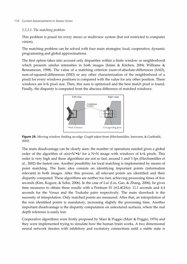
Current Advancements in Stereo Vision 110
2.2.2.1. The matching problem
This problem is posed for every stereo or multiview system (but not restricted to computer vision).
The matching problem can be solved with four main strategies: local, cooperative, dynamic programming and global approximations.
The first option takes into account only disparities within a finite window or neighborhood which presents similar intensities in both images (Islam & Kitchen, 2004; Williams & Bennamoun, 1998). The value of a matching criterion (sum-of-absolute-differences (SAD), sum-of-squared-differences (SSD) or any other characterization of the neighborhood of a pixel) for every windows positions is compared with the value for any other position. These windows are k×k pixel size. Then, this sum is optimized and the best match pixel is found. Finally, the disparity is computed from the abscissa difference of matched windows:
Figure 24. Moving window finding an edge. Graph taken from (Hirchsmüller, Innocent, & Garibaldi, 2002)
The main disadvantage can be clearly seen: the number of operations needed gives a global order of the algorithm of o(n)=N3•k4 for a N×N image with windows of k×k pixels. This order is very high and these algorithms are not so fast, around 1 and 5 fps (Hirchsmüller et al., 2002) the fastest one. Another possibility for local matching is implemented by means of point matching. The basic idea consists on identifying important points (information relevant) in both images. After this process, all relevant points are identified and their disparity computed. These algorithms are neither too fast, achieving processing times of few seconds (Kim, Kogure, & Sohn, 2006). In the case of Lui (Liu, Gao, & Zhang, 2006), he gives time measures to obtain these results with a Pentium IV (@2.4GHz): 11.1 seconds and 4.4 seconds for the Venus and the Tsukuba pairs respectively. The main drawback is the necessity of interpolation. Only matched points are measured. After that, an interpolation of the non identified points is mandatory, increasing slightly the processing time. Another important disadvantage is the disparity computation on untextured surfaces, where the real depth reference is easily lost.
Cooperative algorithms were firstly proposed by Marr & Poggio (Marr & Poggio, 1976) and they were implemented trying to simulate how the human brain works. A two dimensional neural network iterates with inhibitory and excitatory connections until a stable state is

Depth Estimation – An Introduction 111
reached. Later, some other proposals in this group have been proposed (Mayer, 2003; Zitnick & Kanade, 2000).
Dynamic programming strategy consists on assuming the ordering constraint as always true (Käck, 2004). The matching is done line by line, although the independent match of horizontal lines produces horizontal “streaks”. The problem with the noise sensitivity of this proposal is smoothed with vertical edges (Ohta & Kanade, 1985) or ground control points (Bobick & Intille, 1999). These are some of the fastest proposals, achieving around 50 fps in a 3 GHz CPU (Kamiya & Kanazawa, 2008)
Global algorithms make explicit smoothness assumptions converting the problem in an optimization one. They seek a disparity assignment that minimizes a global cost or energy function that combines data and smoothness terms (Scharstein & Szeliski, 2002; Käck, 2004):
E(d)=Edata(d)+ λ•Esmooth(d) (2)
Some of the best results with global strategies have been achieved with the so called graph cuts matching. Graph cuts extends the 1D formulation of dynamic programming approach to 2D, assuming a local coherence constraint, i.e. for each pixel, neighbourhoods have similar disparity. Each match is taken as a node and forced to fit in a disparity plane, connected to their neighbours by disparity edges and occlusion edges, adding a source node (with lower disparity) and a sink node (highest disparity) connected to all nodes. Costs are assigned to matches, and mean values of such costs to edges. Finally, we compute a minimum cut on the graph, separating nodes in two groups and the largest disparity that connect a node to the source is assigned to each pixel (Käck, 2004).
We can find also a group using some specific features of the image, like edges, shapes and curves (Schimd et al., 1999; Szumilas, Wildenauer, & Hanbury, 2009; Xia, Tung, & Ji, 2001). In this family, a differential operator must be used (typically Laplacian or Laplacian of Gaussian, as in (Pajares, Cruz, & López-Orozco, 2000; Jia et al., 2003)). This task requires a convolution of 3×3, 5×5 or even bigger windows; as a result, the computing load increases with the size of the operator (for separable implementations). However, these algorithms allow real-time implementations.
Another possibility of global algorithms are those of Belief propagation (Sun, Shum, & Zheng, 2002), modelling smoothness, discontinuities and occlusions with three Markov Random Fields and itinerates finding the best solution of a “Maximum A Posteriori” (MAP).
A final family of global algorithms to be referred in this study is the segment-based algorithms. This group of algorithms chops the image as explained in equation 1 to match regions. An initial pair of images is smoothed and segmented in regions. The aim of this family of algorithms addresses the problem of untextured regions. After forcing pixels to fit in a disparity plane, the depth map estimation is obtained.
These algorithms have the advantage of producing a dense depth map, disparity estimated at each pixel (Scharstein & Szeliski, 2002), hence, avoiding interpolation. Some algorithms also perform a k×k window pre-match, and a plane fitting, producing a high computational

Current Advancements in Stereo Vision 112
load (and computation time of tens of seconds), and avoiding its use in real-time applications (Bleyer & Gelautz, 2005).
Combinations of segment-based and graph cuts algorithms have also been implemented (Hong & Chen, 2004).
A further group of global algorithms are based on wavelets, as described in (Xia et al., 2001). These algorithms present important problems in terms of time performance, around hours in 3 GHz CPU for two images matching (Radhika et al., 2007).
Summarizing, each of the previously described approaches to the matching problem presents several computing problems. In the case of edges, curves and shapes, differential operators increase the order linearly with the size (for separable implementations). This problem gets worse when using area-based matching algorithms, following the computational load an exponential law. The use of a window to analyze and compare different regions is seen to perform satisfactorily (Bleyer & Gelautz, 2005) however this technique requires many computational resources. Even most of segment-based matching algorithms perform a N×N local windowing matching as a step of the final depth map computation (Hong & Chen, 2004; Scharstein & Szeliski, 2002). It is important to notice that this step is not dimensional separable. Most of these algorithms, however, obtain very accurate results, with the counterpart of interpolating optimized planes that forces to solve linear systems (Hong & Chen, 2004; Klaus, Sormann, & Kraner, 2006). The calculations required for depth mapping of images is very high. It has been studied in detail, and a complete review of algorithms performing this task by means of stereovision can be found at (Scharstein & Szeliski, 2002).
Figure 25 shows some results of the presented algorithms.
(a) (b)
(c) (d)

Depth Estimation – An Introduction 113
(e) (f)
(g) (h)
Figure 25. (a) Ground truth of the Tsukuba scene (Scharstein & Szeliski, 2002), (b) Window 9x9 SAD matching (Hirchsmüller, 2001), (c) points matching (Liu, Gao, & Zhang, 2006), (d) cooperative algorithm (Zitnick & Kanade, 2000), (e) graph cuts depth estimation (Kolmogorov & Zabih, 2010), (f) Belief propagation (Sun et al., 2002), (g) segment regions and plane fitting (Bleyer & Gelautz, 2005), (h) dynamic programming (Scharstein & Szeliski, 2002).
In (Scharstein & Szeliski, 2002) a detailed stereo matching taxonomy can be found.
2.2.2.2. Stereo vision structure
The set of images used to compute the depth can be taken in many different ways, attending to their spatial organization. The first group being analyzed will be the stereo vision. This setup requires two cameras, closely placed and pointing to the scene. The figure 9 shows the general structure of a stereo vision images acquisition.
However, the stereo setup structure presents some free parameters, which may change the way the images should be analyzed. We have already seen some constraints, which allow some simplifications and, thus, fast algorithms, to extract the depth map, such as the fronto-parallel hypothesis (figure 11).
Stereo vision, as defined, allows obtaining a 2.5D image (or a 3D fragmented reconstruction, as it is shown in figure 3). Depending on how much are the image sensors are separated, we will be able to reconstruct more or less points of the volume analyzed. Following (Seitz & Kim, 2002), we can talk about central perspective stereo (when the displacement between both images is done in one single axis) and multiperspective stereo (otherwise). Regarding this last case, (Ishuguro, Yamamoto, & Tsuji, 1992) demonstrated how any perspective can be transformed to a stereo scene, under some geometrical and optical restrictions. In such case, the image rectification and dewrapping is mandatory.

Current Advancements in Stereo Vision 114
2.2.2.3. 2 Multiview structure
The final case that we will present is the multiview setup. In this option, several cameras are placed around the scene, which is captured from different points of view. See figure 26 for an example.
Figure 26. Multiview scheme (Kim, Kogure, & Sohn, 2006).
The algorithms dealing with this scheme need to perform a high number of matches, obtaining, however, a full 3D model, which is not restricted to a single perspective.
3. Conclusions The depth is an important cue of a scene, which is lost in standard image acquisition systems. For that reason, and given that many applications need this information, several strategies have been proposed to extract the depth.
We have seen active methods, which project some energy onto the scene to process the reflections, and passive methods, only dealing with the natural received energy from the scene. Among this last option, we found monocular systems, working with a single perspective, and stereo or multiview systems, which work with more than one single perspective.
We have shown why these last algorithms have to solve the matching problem, or finding the same physical points in two or more images. Several strategies, again, are available in this category.
The analysis has revealed advantages and disadvantages in every system, regarding energy needs, computational load and, hence, speed, complexity, accuracy, range, hardware implementation or price, among others. Thus, there is not a concluding winner among all the analyzed solutions. Instead of that, we will have to think about the final application of our algorithm, to make the correct choice.
Author details
Pablo Revuelta Sanz, Belén Ruiz Mezcua and José M. Sánchez Pena Carlos III University of Madrid, Spain

Depth Estimation – An Introduction 115
Acknowledgement
We would like to acknowledge the student grant offered by the Carlos III University of Madrid and the Spanish Center for Subtitling and Audiodescription (CESyA) which has allowed this research work to be performed.
4. References Albrecht, P. and Michaelis, B. (1998). Improvement of the Spatial Resolution of an Optical 3-
D Measurement Procedure. IEEE Transactions on Instrumentation and Measurement, Vol.47, pp. 158-162.
Benjamin, J. M. Jr. (1973). The Laser Cane. Bulletin of Prosthetics Research, pp. 443-450. Bleyer, M. (2006). Thesis: “Segmentation-based Stereo and Motion with Occlusions”,
Institute for Software Technology and Interactive Systems, Vienna University of Technology.
Bleyer, M. and Gelautz, M. (2005). A layered stereo matching algorithm using image segmentation and global visibility constraints. Journal of Photogrammetry & Remote Sensing, Vol.59, pp. 128-150.
Bobick, A. & Intille, S. (1999). Large occlusion stereo. International Journal of Computer Vision,Vol. 33, pp. 181-200.
Delage, E., Lee, H., & Ng, A. Y. (2005). Automatic single-image 3D reconstructions of indoor Manhattan world scenes. In: 12th International Symposium of Robotics Research (ISRR), pp.305-321.
Douglas, T. S., Solomonidis, S. E., Sandham, W. A., and Spence, W. D. (2002). Ultrasound image matching using genetic algorithms. Medical and Biological Engineering and Computing, Vol.40, pp. 168-172.
Espindola, G. M., Camara, G., Reis, I. A., Bins, L. S., and Monteiro, A. M. (2006). Parameter selection for region-growing image segmentation algorithms using spatial autocorrelation. International Journal of Remote Sensing, Vol.27, pp. 3035-3040.
François, A. R. J. and Medioni, G. G. (2001). Interactive 3D model extraction from a single image. Image and Vision Computing, Vol.19, pp. 317-328.
Gao, L., Jiang, J., and Yang, S. Y. (2006). Constrained Region-Growing and Edge Enhancement Towards Automated Semantic Video Object Segmentation. Lecture Notes in Computer Science, Advanced Concepts for Intelligent Vision Systems, Vol.4179, pp. 323-331.
Georgeson, M. (1976). Antagonism between Channels for Pattern and Movement in Human Vision. Nature, Vol.259, pp. 412-415.
Guttman, S., Gilroy, L. A., and Blake, R. (2007). Spatial grouping in human vision: Temporal structure trumps temporal synchrony. Vision Research,Vol. 47, pp. 219-230.
He, Z. & Wang, Q. (2009). A Fast and Effective Dichotomy Based Hash Algorithm for Image Matching. Lecture Notes in Computer Science, Advances in Visual Computing, Vol. 5358, pp. 328-337.
Helmi, F. S. & Scherer, S. (2001). Adaptive Shape from Focus with an Error Estimation in Light Microscopy. 2nd Int'l Symposium on Image and Signal Processing and Analysis, pp. 188-193.

Current Advancements in Stereo Vision 116
Hirchsmüller, H. (2001). Improvements in real-time correlation-based stereo vision. In: IEEE Workshop on Stereo and Multi-Baseline Vision at IEEE Conference on Computer Vision and Pattern Recognition, December 2001, Kauai, Hawaii, pp. 141-148.
Hirchsmüller, H., Innocent, P. R., and Garibaldi, J. (2002). Real-Time Correlation-Based Stereo Vision with Reduced Border Errors. Journal of Computer Vision, Vol. 47, pp. 229-246.
Hong, L. & Chen, G. (2004). Segment-based Stereo Matching Using Graph Cuts. Computer Vision and Pattern Recognition (CVPR) 2004. Proceedings of the 2004 IEEE Computer Society Conference on, Vol. 1, pp. I-74-I-81.
Ishuguro, H., Yamamoto, M., & Tsuji, S. (1992). Omni-directional stereo. PAMI, Vol.14, pp. 257-262.
Islam, M. S. & Kitchen, L. (2004). Nonlinear Similarity Based Image Matching. International Federation for Information Processing, Vol.228, pp. 401-410.
Jacobs, G. H., Williams, G. A., Cahill, H., and Nathans, J. (2007). Emergence of Novel Color Vision in Mice Engineered to Express a Human Cone Photopigment. Science, Vol.315, pp. 1723-1727.
Jia, Y., Xu, Y., Liu, W., Yang, C., Zhu, Y., Zhang, X. et al. (2003). A Miniature Stereo Vision Machine for Real-Time Dense Depth Mapping. Lecture Notes in Computer Science, Computer Vision Systems, Vol.2626, pp. 268-277.
Käck, J. (2004). Robust Stereo Correspondence using Graph Cuts. Master Thesis, Royal Institute of Technology. Available from:
www.nada.kth.se/utbildning/grukth/exjobb/rapportlistor/-2004/rapporter04/kack per-jonny 04019.pdf
Kamiya, S. & Kanazawa, Y. (2008). Accurate Image Matching in Scenes Including Repetitive Patterns. Lecture Notes in Computer Science, Robot Vision, Vol.4931, pp. 165-176.
Kim, H. K. I., Kogure, K., & Sohn, K. (2006). A Real-Time 3D Modeling System Using Multiple Stereo Cameras for Free-Viewpoint Video Generation. Lecture Notes in Computer Science, Image Analysis Recognition, Vol.4142, pp. 237-249.
Kim, J. Ch., Lee, K. M., Choi, B. T., & Lee, S. U. (2005). A dense stereo matching using two-pass dynamic programming with generalized ground control points. In: Computer Vision and Pattern Recognition (CVPR) 2005. IEEE Computer Society Conference on, pp. 1075-1082
Klaus, A., Sormann, M., and Kraner, K. (2006). Segment-Based Stereo Matching Using Belief Propagation and a Self-Adapting Dissimilarity Measure. Pattern Recognition (ICPR) 2006. 18th International Conference on, pp. 15-18.
Kolmogorov, V. & Zabih, R. (2010). Computing visual correspondence with occlusions via graph cuts. Rep. No. Technical Report CUCS-TR-2001-1838, Cornell Computer Science Department.
Kostková, J. & Sára, R. (2006). Fast Disparity Components Tracing Algorithm for Stratified Dense Matching Approach. Rep. No. Research Reports of CMP, Czech Technical University, No. 28.
Kurki, I. & Saarinen, J. (2004). Shape perception in human vision: specialized detectors for concentric spatial structures?. Neuroscience Letters, Vol.360, pp. 100-102.

Depth Estimation – An Introduction 117
Liu, L., Gao, H.-B. & Zhang, Q. (2006). Research of Correspondence Points Matching on Binocular Stereo Vision Measurement System Based on Wavelet. CORD Conference Proceedings, pp. 3687-3691. Available from:
http://pubget.com/paper/pgtmp_a32b66de88e2f5adb012c343cb5f2bf4 Malik, A. S. & Choi, T.-S. (2008). Depth Estimation by Finding Best Focused Points Using
Line Fitting. Lecture Notes in Computer Science, Image and Signal Processing, Vol.5099, pp. 120-127.
Marr, H. & Poggio, T. (1976). Cooperative computation of stereo disparity. Science, Vol.194, pp. 283-287.
Mayer, H. (2003). Analysis of means to improve cooperative disparity estimation. ISPRS Conference on Photogrammetric Image Analysis, JSPRS Archives, Vol.XXXIV, Part 3/W8.
Meese, T. S. & Summers, R. J. (2009). Area summation in human vision at and above detection threshold. In: Proceedings of the Royal Society B: Biological Sciences, Vol.274, pp. 2891-2900.
Mesa Imaging. (2011). SR4000 Data Sheet. 20-1-2012. Avaliable from: http://www.mesa-imaging.ch/pdf/SR4000_Data_Sheet.pdf
Nagai, T., Naruse, T., Ikehara, M., & Kurematsu, A. (2002). Hmm-based surface reconstruction from single images. In. Image Processing. 2002. Proceedings. 2002 International Conference on, Vol.2, pp. II-561 - II-564
Nathans, J. (1999). The Evolution and Physiology of Human Color Vision: Insights from Molecular Genetic Studies of Visual Pigments. Neuron, Vol.24, pp. 299-312.
ODOS Imaging. (2012). 2+3D™ - real world in real time. 20-1-2012. Available from: http://odos-imaging.com/
Ohta, Y. & Kanade, T. (1985). Stereo by intra- and inter-scanline search using dynamic programming. IEEE Transactions on Pattern Analysis and Machine Intelligence, Vol.7, pp. 139-154.
Ozden, K. E., Schindler, K., and van Gool, L. (2007). Simultaneous Segmentation and 3D Reconstruction of Monocular Image Sequences. Computer Vision, 2007. ICCV 2007. IEEE 11th International Conference on, pp. 1-8.
Pajares, G., Cruz, J. M., and López-Orozco, J. A. (2000). Relaxation labeling in stereo image matching. Pattern recognition, Vol.33, pp. 53-68.
Pham, D. L., Xu, C., and Prince, J. L. (2000). Current Methods in Medical Image Segmentation. Annual Review of Biomedical Engineering, Vol.2, pp. 315-337.
Pons, J.-P. & Keriven, R (2007). Multi-View Stereo Reconstruction and Scene Flow Estimation with a Global Image-Based Matching Score. International Journal of Computer Vision, Vol.72, pp. 179-193.
Racheva, K. & Vassilev, A. (2009). Human S-Cone Vision Effect of Stiumuls Duration in the Increment and Decrement Thresholds. Comptes rendus de l'Academie bulgare des Sciences, Vol.62, pp. 63-68.
Radhika, V. N, Kartikeyan, B., Krishna, G., Chowdhury, S., and Srivastava, P. K. (2007). Robust Stereo Image Matching for Spaceborne Imagery. IEEE Transactions on Geoscience and Remote Sensing, Vol.45, pp. 2993-3000.
Rangarajan, S. (2005), Algorithms for Edge Detection, Stony Brook University. Available from: www.uweb.ucsb.edu/~shahnam/AfED.doc

Current Advancements in Stereo Vision 118
Revuelta Sanz, P., Ruiz Mezcua, B., Sánchez Pena, J. M., & Thiran, J.-P. Stereo Vision Matching over Single-channel Color-based Segmentation, In: International Conference on Signal Processing and Multimedia Applications (SIGMAP) 2011 Proceedings, pp. 126-130.
Saxena, A., Chung, S. H., and Ng, A. Y. (2008). 3-D Depth Reconstruction from a Single Still Image. International Journal of Computer Vision, Vol.76, pp. 53-69.
Scharstein, D. & Szeliski, R. (2002). A Taxonomy and Evaluation of Dense Two-Frame Stereo Correspondence Algorithms. International Journal of Computer Vision, 47, 7-42.
Scharstein, D. & Szeliski, R. (2003). High-Accuracy Stereo Depth Maps Using Structured Light. In: IEEE Computer Society Conference on Computer Vision and Pattern Recognition (CVPR) 2003, Vol.1, pp. 195-202, Madison, WI.
Scharstein, D. Middlebury Database. (2010). www.middlebury.edu/stereo Schimd, C., Zisserman, A., & Mohr, R. (1999). Integrating Geometric and Photometric
Information for Image Retrieval. Lecture Notes in Computer Science, Shape, Contour and Grouping in Computer Vision, Vol.1681, pp. 217-233.
Schuon, S., Theobalt, Ch., Davis, J., & Thrun, S. (2008). High-quality scanning using time-of-flight depth superresolution. In: IEEE CVPR Workshop on Time-Of-Flight Computer Vision 2008, pp. 1-7
Seitz, S. M. & Kim, J. (2002). The Space of All Stereo Images. International Journal of Computer Vision, Vol.48, pp. 21-38.
Stromeyer, C. F., Kronauer, R. E., Madsen, J. C., and et al. (1984). Opponent-Movement Mechanisms in Human-Vision. Journal of the Optical Society of America A-Optics Image Science and Vision, Vol.1, pp. 876-884.
Sun, J., Shum, H.-Y., and Zheng, N.-N. (2002). Stereo matching using belief propagation. In: European Conference on Computer Vision, pp. 510-524.
Szumilas, L., Wildenauer, H., & Hanbury, A. (2009). Invariant Shape Matching for Detection of Semi-local Image Structures. Lecture Notes in Computer Science, Image Analysis Recognition, Vol.5627, pp. 551-562.
Tuytelaars, T. & Gool, L.V. (2004). Matching Widely Separated Views Based on Affine Invariant Regions. International Journal of Computer Vision, Vol.59, pp. 61-85.
Wang, Ch. & Gavrilova, M. L. (2005). A Novel Topology-Based Matching Algorithm for Fingerprint Recognition in the Presence of Elastic Distortions. Lecture Notes in Computer Science, Computational Science and Its Applications ICCSA, Vol.3480, pp. 748-757.
Wang, X. L. & Wang, L. J. (2008). Color image segmentation based on Bayesian framework and level set. Proceeding of 2008 International Conference on Machine Learning and Cybernetics, Vol.1, No.7, pp. 3484-3489.
Williams, J. & Bennamoun, M. (1998). A Non-linear Filtering Approach to Image Matching. In: Proceedings of the 14th International Conference on Pattern Recognition, Vol.1, No.1, p. 3.
Xia, Y., Tung, A., and Ji, Y. W. (2001). A Novel Wavelet Stereo Matching Method to Improve DEM Accuracy Generated from SPOT Stereo Image Pairs. International Geoscience and Remote Sensing Symposium, Vol.7, pp. 3277-3279.
Yu, J., Weng, L., Tian, Y., Wang, Y., and Tai, X. (2008). A Novel Image Matching Method in Camera-calibrated System. In: Cybernetics and Intelligent Systems, 2008 IEEE Conference on, pp. 48-51.
Zitnick, L. & Kanade, T. (2000). A cooperative algorithm for stereo matching and occlusion detection. IEEE Transactions on Pattern Analysis and Machine Inteligence, Vol.22, pp. 675-684.

Chapter 0
An Overview of Three-Dimensional Videos:3D Content Creation, 3D Representationand Visualization
Lourena Rocha and Luiz Gonçalves
Additional information is available at the end of the chapter
http://dx.doi.org/10.5772/50177
1. Introduction
The upcoming of digital video has caused a technological revolution that has changedaudiovisual communication in several ways. The digital format, in its essence, is appropriateto computational processing. As a consequence, it has a huge impact in the cinema andtelevision industries. Nowadays, with advances experimented in Internet and wirelessnetworking, digital video has been consolidated as a new and important media. For example,the Skype application relies in this kind of media in order to allow partners that are distant faraway communicate to each other.
Current generation of digital video brings revolutionary aspects as the incorporation of newdata types in the media. Depth information is certainly one data type that is typicallynatural, inserted in digital videos in order to provide more realism. That is, the insertionof depth agrees with human perceptual system and also makes easier the scene analysisusing computers, mainly if the goal is to extract high-level information. In this way,three-dimensional video (or simply 3D video) comes up, used to reproduce images inmovement with the third dimension sensation or to recreate a dynamic scene visualizationwith other viewpoints besides the one that the movie has been filmed. 3D videos that allowthe scene visualization from new viewpoints can be constructed using an image or modelbased approach. These type of 3D videos are known as free-viewpoint video, or so-calledFVV, and 3D videos providing depth perception are so-called 3DV or stereoscopic videos.
So, in the scope of this text, the main characteristic of a 3D video is that it captures thedynamics and movement of the scene during the filming, offering to the user the possibilityto change the point of view during the exhibition, beyond supplying the three-dimensionalmodel of visualized objects. Automatic construction of three-dimensional photo-realisticmodels of a scene is important in applications such as interactive visualization of environment
Chapter 6

2 Stereo Vision
or objects that are remotely located, for example. One could provide a modification ofa real scene for virtual reality tasks. Other applications of 3D video are in Archeology,Oceanography, Historic and Cultural Sites, Arts, Education and Entertainment.
In general, an end-to-end 3D video system pipeline consists of the following stages:capture system setup, 3D reconstruction, 3D representation, coding, transmission, decoding,rendenring and 3D display. They can be classified in four main blocks: 3D Content Creation(capture and 3D recontruction stages), 3D Representation, Delivery (coding, transmission anddecoding stages) and Visualization (rendering and 3D display stages).
In this text, we provide an extensive literature review on 3D Content Creation, 3DRepresentation and Visualization blocks of the 3D video pipeline. The Delivery blockregarding coding, transmission and decoding techniques is not in the scope of this text.It is mainly intended for applications involving some network channels, such as, internetapplications and 3D TV.
3D videos are one of the most active research topics and other reviews have already beenproposed [63, 66, 74].
The chapter is organized as follows. Section 2 explains the pipeline of 3D videos fromcapture to display. As part of the 3D Content Creation block, we discuss acquisitionsystems and 3D reconstructions techniques in Section 3. Section 4 presents the most popular3D representations formats in the context of 3DV and FVV. The Visualization block, withrendering and 3D display stages, is discussed in Section 5. Finally, Section 6 concludes thechapter.
2. Pipeline of 3D video systems
3D videos are now a huge success due to the release of Avatar film in 2010. Besides its use incinemas, applications that require some sort of 3D video transmission, such as internet and3D TV is also receiving attention. 3D TV, for example, is a reality and the first 3D commercialchannels are available.
For such sort of applications, an end-to-end 3D video system is subdivided into four mainblocks: 3D Content Creation, 3D Representation, Delivery and Visualization (see Fig. 1).
Figure 1. Pipeline of an end-to-end 3D video system.
The 3D Content Creation block (Fig. 2) is responsible for providing the data used to create the3D video. The process starts at the Capture stage (Subsec. 3.1) with the choice of equipmentsthat will be used to capture the scene and process data. Examples of devices for scene captureare 3D scanners, time-of-flight (TOF) sensors and digital cameras. The latter is the most widelyused for capturing dynamic scenes, sometimes combined with other sensors. Other necessaryequipments are computers, disks, grabber cards, etc. Projectors are also used in some systems
120 Current Advancements in Stereo Vision

An Overview of Three-Dimensional Videos:3D Content Creation, 3D Representation and Visualization 3
to improve the quality of captured data. The number of cameras in a setting varies and itdepends on the application, as well as, its costs. For example, in literature we can find systemswith more than 50 cameras [28] and also systems composed by only one camera and oneprojector [81].
After capture stage the data is sent to post-processing where low-level algorithms are appliedto correct and improve data accuracy. For example, algorithms for color correction, correctionof lens distortion and keystone distortion, camera calibration, features extraction and tracking,image rectification and alignment are within this stage. For explanations on these algorithms,we refer the reader to any Computer Vision book, such as the one in [75].
The processed data is sent to the 3D Reconstruction stage. The 3D reconstruction problemrefers to the recovering of scene geometry, i.e., the 3D coordinates of objects that composethe scene. This stage is responsible for creating the data that will be used withinthe 3D video representation. Common techniques performed for geometry recovery arestructure-from-stereo, shape-from-silhouette, structure-from-motion, shape-from-focus anddefocus, as well as, shape-from-shading. In Subsection 3.2 we will discuss structure fromstereo, structure from motion and shape from silhoettes techniques in the context of 3DVand FVV. Structure-from-stereo methods are the most popular in 3D videos literature andhave been investigated by the MPEG group for standardization. Another research line on 3Dreconstruction fuses data obtained from digital cameras and ToF sensors [29, 89].
A review of dynamic scenes capture can be found in [72].
Figure 2. 3D Content Creation block. Sensors capture the scene and the acquired data is processed bylow-level algorithms in Post-Processing stage. 3D reconstruction method is applied in order to createdata that will be used by the 3D representation.
At the 3D Representation stage (Section 4) a format is chosen to store data from the 3DContent Creation block. There are a variety of 3D representation schemes in literature [64].Its choice depends on the target application and capture devices. They can be classifiedin image-based (Subsec. 4.1), geometry-based (Subsec. 4.2) and a representation based ondepth maps (Subsec. 4.3), which combines image and geometry aspects [63]. Geometry-basedformats represent data as we know from Computer Graphics. They offer a full navigation ofthe scene or object, but it has realistic rendering issues due to errors in reconstruction step.
121An Overview of Three-Dimensional Videos: 3D Content Creation, 3D Representation and Visualization

4 Stereo Vision
On the other hand, image-based formats avoid the explicit 3D reconstruction of the scene andprovides a more realistic visualization. Depth-maps formats are more suitable for 3DV andFVV coding and has been investigated for standardization by the MPEG group.
Figure 3. Categorization of 3D Representation formats.
The Delivey block is responsible for 3D video coding, transmission and decoding. Usually, itis necessary in applications with some type of network, such as Internet and 3D TV. Moreover,coding and decoding of 3D videos are important for development of storage media, e.g.,Blu-ray discs. These are not in the scope of this text. We refer the reader interested in codingof 3D videos to the works in [64, 65, 80]. Readers interested in transmission and also storageof 3D videos are refered to references [22, 57]. A discussion about technologies to deliver 3Dcontent to mobile devices can be found in [20].
The last building block of a 3D video system is the most important to the end user, becauseit deals with Visualization of the 3D content. It comprises Rendering stage and 3D Displays(Fig. 4). The Rendering stage 5.1 is responsible for employing algorithms to render the datastored at the representation format. The main focus is the view synthesis methods. They arenecessary for free view point functionality and autoestereoscopic displays. More than othersstages, this one is in charge of providing a realistic view of 3D dynamic scenes. Of course, itsperformance depends on several factors, such as the accuracy of the reconstructed data anddata loss during transmission. In a 3D TV scenario it also depends on the receiver processingcapability.
Figure 4. Visualization
3D Displays (Subsec. 5.2) are responsible for depth perception of stereoscopic videos. Also,for free-viewpoint videos they have to be able to provide means of interaction with thevisualized content. 3D displays technologies are in constant development since 3D mediabecame more accessible to home user. Specialists in consumer electronics predict that in 2015
122 Current Advancements in Stereo Vision

An Overview of Three-Dimensional Videos:3D Content Creation, 3D Representation and Visualization 5
more than 30% of all high-definition panels at home will be equipped with 3D capabilities.Stereoscopic videos technologies are mature and a huge success in cinemas, but there is roomfor improvement, specially regarding 3D displays. Stereoscopic displays are the most popular3D display in the market, but in order to provide depth perception they require the use ofuncomfortable glasses. To overcome this limitation, researches on autostereoscopic displaysare under development. Autostereoscopic displays allow depth perception and FVV with norequirement of eyewear. Other types of 3D displays are holography and integral imaging.We refer readers interested in advances in holography and integral imaging to references [51]and [7], respectively.
3. 3D content creation
3.1. Capture
There are a variety of technologies for digitally acquiring the geometry of a 3D object. Thechoice of the acquisition setup strongly depends on the application, and of course, its costs.Digital cameras, 3D laser scanners and time-of-flight (TOF) sensors are the most populardevices for geometry and color acquisition.
An important laser scanner system has been presented in [55]. It utilizes a laser triangulationscanner and a high-resolution color camera to scan the 5m tall Davi, a sculpture ofMichelangelo. Structured light scanners settings are composed by a projector and one ormore cameras [3, 73]. In these systems a pattern is projected onto the object surface in orderto improve the quality of the captured 3D object coordinates. In reference [9] the authorspropose the scanning of 3D objects using a ToF camera. All systems cited above capture 3Dinformation of static scenes. Figure 5 shows the simple acquisition setup utilized to capturethe geometry of Parthenon sculptures [73].
Figure 5. Simple structured light scanner consisting of a digital camera, a projector and a tripod usedin [73] and, on the right, a sculpture model obtained after 14 scans.
For dynamic scenes the most used devices are digital cameras. Systems with one or twocameras can be found in literature. For example, in reference [52] scene structure and motion
123An Overview of Three-Dimensional Videos: 3D Content Creation, 3D Representation and Visualization

6 Stereo Vision
are retrieved using a hand-held camera and a real-time 3D system with a high-definitioncamera and a projector is presented in [81]. However, most settings utilize several digitalcameras as in [26], for example. The concept of 3D video bricks was introduced in [82]. One 3Dvideo brick is composed by a projector, two black-and-white cameras and a high-definitioncolor camera. The complete setting comprises multiple 3D video bricks.
Cameras can be arranged in a parallel or convergent setup (see Figure 6). One of thepioneering projects in this area is presented in reference [26]. The 3D Dome Studio uses 51cameras mounted on a 5m diameter dome and applies stereo techniques to reconstruct theshape of a moving object. The same techniques have been used in a circular setup with morethan 30 cameras to shoot a football game. All cameras are sinchronized and pointing to thesame target from different angles. The set of captured multi-view images are processed anda 3D model is reconstructed. In reference [6], 7 cameras where placed in a convergent fixedsetup pointing to the center of the scene. Cameras are synchronized and calibrated. The maingoal is the reconstruction and rendering of human bodys from any viewpoint and estimateits motion parameters. Another curved setting can be found in [40] where 12 cameras whereplaced at the ceiling, around the scene.
An example of parallel setup can be seen in [58]. It uses six consumer quality Fire-Wire videocameras aligned in two rows. Cameras where partitioned in stereo pairs, and every stereo pairis connected to one PC for stereo processing. The 3D system in [76] captures dynamic eventswith several cameras displaced in sequence and generates novel views with interpolationmethods. Another example of parallel camera arrangement can be seen in [43].
Figure 6. Example of convergent setup with 51 cameras proposed in [26] (left) and a parallel one with 16cameras in [43] (right).
All studio settings shown above use controled illumination to facilitate reconstructionprocesses. As a consequence, studio setups rigorously restricts the type of observed scene.In [8] authors use auto-exposure and gain changes compensation in order to capture outdoorscenes which has a large variation in illumination. The setup is portable and can be hold ina backpack or vehicle mount. It consists of a GPS, an inertial sensor and an omnidirectionalcamera, with six cameras within (see Fig. 7).
124 Current Advancements in Stereo Vision

An Overview of Three-Dimensional Videos:3D Content Creation, 3D Representation and Visualization 7
Figure 7. On the left the backpack mount. On the right the sensors head with GPS, inertial sensor andthe omniderctional camera. Figures taken form [8]
Recently a new system configuration has been investigated. These 3D systems employs sensorfusion combining depth sensors and digital cameras [29, 90]. Their main goal is obtain moreaccurate depth maps by combining stereo methods and data acquired by depth sensors.
Commercial solutions for ease 3D acquisition are available. They are called stereo- or 3Dcameras. Figure 8 shows the stereo camera Bumblebee XB3 from Point Grey Research andthe full-HD professional 3D Panasonic AG-3DA1. Both cameras are available at NatalnetLaboratory. Bumblebee XB3 has a 3-sensor multi-baseline with variable resolutions and comewith softwares for stereo processing. The Panasonic AG-3DA1 has integrated twin-lens andrecords and process synchronized left and right streams. The recorded channels are stored onmemory cards in AVCHD format.
Figure 8. Bumblebee XB3 from Point Grey Research (left) and full-HD professional 3D PanasonicAG-3DA1 (right).
3.2. 3D reconstruction
After images are captured and pre-processed they are sent to the reconstruction stage. The 3Dreconstruction problem refers to the recovering of scene geometry, i.e., the 3D coordinates ofobjects that compose the scene. This stage is responsible for creating the data that will be usedwithin the 3D video representation.
125An Overview of Three-Dimensional Videos: 3D Content Creation, 3D Representation and Visualization

8 Stereo Vision
3D video systems in literature differ on the employed reconstruction methods. Examples ofsuch methods are shape from focus, shape from shading, structure from motion, shape fromsilhouette and structure from stereo. We refer the reader to any Computer Vision book [75] fora broad discussion about existing reconstruction methods. However, structure-from-stereotechniques have shown be more suitable for 3DV and FVV [68].
Here we will review some works of structure-from-stereo, structure-from-motion andshape-from-silhouette techniques within the context of 3D videos.
3.2.1. Structure from stereo
The most popular method of 3D reconstruction is stereo [78]. It is based in the principle ofstereo vision (or stereopsis) which copes with the human visual system [38]. Because of theposition of our eyes, our brain receives two views of a same scene from two slightly differentviewpoints at the same horizontal level. Our brains fuse these two images and measure thedisparity in order to estimate depth [38]. Computationally, stereo process has three mainsteps: selection of a particular location of the surface in one image (feature extraction); theselected location must be identified in the other image ( matching or correspondence problem); thedisparity in two correspondent locations must be computed (reconstruction) [38]. The processused to obtain 3D point coordinates from a set of known corresponding image locations iscalled triangulation [75, 78]. Overviews about the problem of recovering 3D structures fromstereo can be found in literature [5, 13].
Over the years many efforts have been made by academics to compute stereo efficiently forstatic and dynamic events. The literature stereo is very extensive. In [56] an important worksurveying and evaluating binocular stereo algorithms has been presented. The authors havecategorized dense binocular stereo according to: matching cost computation, cost aggregation,disparity computation and disparity refinement.
Multiview stereo
For free-viewpoint video development it is mandatory the acquisition of images from manydifferent viewpoints (see Fig. 9). Thus, the problem of reconstructing 3D scenes from morethan 2 frames arises, the so-called multi-view stereo reconstruction problem [23].
Many algorithms to compute multi-view stereo has been developed [72]. A taxonomy formulti-view stereo methods has been proposed [59], similar to the one presented in [56] forbinocular stereo methods evaluation. The multi-view algorithms are classified and evaluatedaccording to six categories: scene representation, photoconsistency measure, visibility model,shape prior, reconstruction algorithm, initialization requirements. According to this taxonomythe reconstruction algorithms can be classified in four mais classes [59]:
• Cost computation on a 3D volume - for example, voxel coloring methods [60];
• Minimization of a cost function - for example, space carving methods [31];
• Computation of depth-maps;
• Extraction and matching of feature points.
126 Current Advancements in Stereo Vision

An Overview of Three-Dimensional Videos:3D Content Creation, 3D Representation and Visualization 9
Figure 9. Example of multi-camera setup (left) and images of a same scene captured from manydifferent viewpoints (right). Figures taken from [63]
In [18] the authors propose a new algorithm to implement multi-view stereo reconstructionby employing a pipeline other than Feature Extraction, Matching and Reconstruction astraditional stereo methods. It starts with a sparse set of matched points that are expanded toa more dense set and filtered using visibility constraints. This process results in a patch-basedrepresentation of the surface which is transformed into a mesh-based representation.
Multiview stereo algorithms have been applied to obtain 3D objects geometry fromphotos [36]. Also, many 3D video systems based on multiview stereo algorithms have beenproposed [44, 82, 84, 92]. In the context of FVV one of the pioneering works can be seenin [26]. The authors use the multi-baseline stereo algorithm of [50] to obtain depth maps thatare edited to remove innacuracys. It reconstructs fore- and back-ground objects. The systemin [27] is also based on the same algorithm.
An recent overview of coding algorithms to stereo and multiview video can be found in [80].
Active stereo
The most difficult part in stereo computation is the matching or correspondence problem [38].Active stereo methos try to overcome this limitation by emitting and projecting some sort ofwaves onto the surface. In structured light approaches a controlled illumination pattern isprojected. This methodology has been applied to obtain 3D models of cultural artifacts, suchas statutes [3, 34, 73].
Many 3DV and FVV systems benefits from this idea [26, 81–84, 92]. In [81], for example, areal-time 3D system is presented. It utilizes only one camera and one projector. They must besynchronized to guarantee that the projected pattern it will be projected at the same time thecamera captures it. Camera and projector have to be calibrated, as well. The projector projectsslides with a sequence of colored stripes and consecutive stripes may not have the samecolor(see Fig. 10). Experiments where made with static and also reasonably fast movementsscenes. The system needs improvements on the quality of reconstructed scenes but it is apromising approach towards real-time 3D video system. Unlike the previous setting, themulti-view stereo system in [82] projects a binary vertical stripes pattern with randomlyvarying stripes width (see Fig. 10).
127An Overview of Three-Dimensional Videos: 3D Content Creation, 3D Representation and Visualization

10 Stereo Vision
Figure 10. Upper row: scene illuminated with colored stripes (left) and the reconstructed scene(right) [81]. Lower row: color image (left) and same image with structured light illumination (right) [82].
Spacetime stereo
Methods to compute depth via triangulation have been widely investigated by the computervision community. Stereo, laser scanning and time- or color- structured light are the mostpopular. Usually they are classified as active or passive methods. In [11] a new classificationof the 3D reconstruction methods based on triangulation is proposed. Instead of passiveor active approaches, the methods would be classified according to the domain wherecorresponding features are located. Techniques such as laser scanning and passive stereoidentify features only in spacial domain. Methods such as time structured light use featuresonly in temporal domain. The spacetime stereo approach looks for features in both spatial andtemporal domains (see Fig 11). This new methodology has been applied for dynamic scenesreconstruction [10, 48].
In parallel, other research groups where also interested in spatio-temporal benefits. Inreference [88] the authors have employed spacetime approach in three different cases. Forstatic scenes they have used structured light to obtain high-quality depth maps and whereobserved improvements over traditional stereo methods. They have tested the spacetimetheory in quasi-static objects such as waterfalls and it proved to be more efficient. For dynamicscenes under natural lighting conditions it behaved like traditional stereo. The approachpresented in [88] have been used to develop a scalable 3D video system [83].
128 Current Advancements in Stereo Vision

An Overview of Three-Dimensional Videos:3D Content Creation, 3D Representation and Visualization 11
Figure 11. Spacetime principle. The search for correspondences in traditional stereo is done in spatialdomain only (left). In spacetime stereo search for correspondences is done in spatial and temporalneighborhoods (right). Figure taken from [48].
In reference [62] the spacetime approach was used to improve the video resolution of dynamicscenes. The super-resolution is obtained simultaneasly in space and time and makes thesystem capable of recovering dynamic events that happens faster than video frame-rate.
3.2.2. Structure from motion
In Computer Vision, the problem of recovering the Structure From Motion (SFM) [75] refers tothe process of finding the three dimensional structure of an object by analyzing its motion overtime. We perceive a lot of information from the three dimensional structure of the environmentby moving around. The same happens when the objects perform some movement in the scene.
The SFM problem is similar to stereo vision. In both approaches, the image correspondencesand the 3D coordinates of the object must be computed. But in SFM, in order to findcorrespondences between images, features such as corners must be tracked from an image toanother. The trajectories of these features are used to reconstruct the 3D object and the cameramotion. Because of features tracking, SFM is especially effective with video sequences.
Most SFM techniques reconstructs scenes with rigid objects, but in [4, 77] the authors dealwith scenes with non-rigid objects, such as animals and humans. A limitation of SFM is thatthe pixels correspondences can only be calculated accurately for salient features.
In [91] the authors use structure from motion to reconstruct statics scenes from a sequence ofuncalibrated images. For such, a hand-held camera is used. They required restrict cameramotion, specially camera rotations. No prior information is required besides the imagesthemselves. One limitation is that it strongly depends on image texture because it is a featurebased approach.
The reconstruction of 3D scenes captured by a hand-held camera was the main goal of otherworks[52, 54], as well. Structure from motion techniques were used to reconstruct citysarchitecture [53]. The authors try to fuse the data obtained by SFM approach and GPSmeasurements.
3.2.3. Shape from silhouette
Many algorithms of 3D reconstruction are based on object’s silhouettes. This class oftechniques are known as Shape-from-Silhouette [75]. The important concept of Visual
129An Overview of Three-Dimensional Videos: 3D Content Creation, 3D Representation and Visualization

12 Stereo Vision
Hull of an object S was introduced in [32] to identify which parts of S are important tosilhouette-based approaches. A formal definition is:
" The visual hull VH(S, R) of an object S relative to a viewing region R is a region of E3
such that, for each point P ∈ VH(S, R) and each viewpoint V ∈ R, the half-line startingat V and passing trough P contains at least a point of S." [32]
For each viewpoint V, the lines starting at V and passing trough P form a silhouette cone.The volume generated by intersecting all silhouette cones from all viewpoints V is the visualhull 12. Volume carving [31] is the approach commonly used for such. Since volumetrictechniques are traditionally slow, an image-based visual hull (IBVH) [42] have been developedto overcome this limitation. It is real-time and like all image-based rendering techniqueit provides a realistic rendering of the scene. It is pertinent to observe that silhouettesapproaches suffer from one important limitation: they are not able to distinguish concavesurface regions. Thus, the reconstruction of concave objects is not guaranteed with silhouetteapproaches only. Efforts to overcome this problem have been made [17], as well.
Figure 12. Intersection of silhouette cones. The result is the visual hull volume. Figure taken from [42]
In the context of 3DV and FVV silhouettes approaches have been widely used to recover the3D object surface. The systems in [39, 40, 45, 67] employ the same volumetric strategy:the visual hull volume is computed, then it is divided in voxels. For each frame andviewing position all voxels are marked as occupied (object portion) or empty (backgroundportion). After this process the remaining voxels contain the object and form a voxel-basedrepresentation of it. Finally, the marching cubes algorithm transforms the voxels model into atriangle mesh, which represents the object surface.
3D video systems using variants of IBVH have been already proposed [21, 85, 86].Reference [37] presents a complete 3DV and FVV system combining visual hull, surfacetexture, image features and inertia constraints to perform a high quality reconstruction ofdynamic scenes.
130 Current Advancements in Stereo Vision

An Overview of Three-Dimensional Videos:3D Content Creation, 3D Representation and Visualization 13
4. 3D video representation
Various representation schemes for 3D videos can be found in literature [64]. Usually its choicedepends on the target application. But for some authors [63] it determines completely the 3Dvideo system design.
3D scene representation formats can be classified in image- and geometry-based formats andalso a hybrid representation based on depth maps (Subsec. 4.3), which combines image andgeometry aspects [63].
Geometry-based modeling (Subsec. 4.2) represents data as we know from Computer Graphics.In order to use this format the 3D scene has to be reconstructed and the geometry stored ina well know format such as, polygonal meshes or point clouds. They offer a full navigationof the scene or object, but it has realistic rendering issues due to errors in reconstruction step.On the other hand, image-based formats (Subsec. 4.1) avoid the explicit 3D reconstruction ofthe scene and provides a more realistic visualization. But there is a critical trade-off betweenrealistic rendering and size of stored data.
4.1. Image-based representation
The popular format of a three-dimensional video is a stereoscopic video composed by twovideo signals, one for each eye. It is the image-based format used by movie theaters andcurrent 3D TV for home entertainment. Due to its simple format it can be encoded usingexisting video codecs, by performing spatial or temporal interleaving. For spatial interleavingthe images for the right and left eye are resized and packed into a single frame. They can bearranged in side-by-side or top-bottom. In a temporal interleaving the right and left imagesare shown in alternate times.
For FVV systems exist Light fields [19, 33] and Ray-space [76] representations. Bothrepresentations do not perform any geometric reconstruction, avoiding the artifacts generatedby this process. Thus, they lead to a more realistic rendering of the scenes. However, therealistic rendering is paid by the cost of the huge amount of necessary data. They need tostore and transmit a set of views that are, at the receiver side, interpolated in order to generatenovel views. If only a few views are transmitted the rendering quality is poor.
4.2. Geometry-based representations
4.2.1. Polygonal meshes
Polygonal meshes [16] are the most popular 3D scene representation in many industriessuch as architecture and entertainment. Due to realism requirements in computer graphicsand the development of 3D scanning technologies, polygonal meshes representing 3Dsurfaces contain millions of polygons. On one hand they can represent satisfactorily almostany geometric detail of the surface. On the other hand these meshes are complex andcomputationally expensive to be stored, transmitted and rendered. To overcome theselimitations, many techniques to compress and simplify complex meshes have been developedleading to progressive approaches [24], even for time-varying meshes [30].
131An Overview of Three-Dimensional Videos: 3D Content Creation, 3D Representation and Visualization

14 Stereo Vision
Important projects that build 3D polygonal mesh models from scanner systems or photoshave been proposed [3, 53]. Many developed 3DV and FVV systems are based on polygonalmesh representation [6, 37, 71]. In [39–41, 45, 67] a triangular mesh is obtained from avoxel representation via marching cubes algorithm, after silhouette-based reconstruction. Inreference [37] instead of marching cubes algorithm the authors perform multi-level partitionof unity implicits (MPLU) [49]. Reference [6] uses a prior body model consisting of 16 closedtriangle meshes. Researchers in [39, 41] present a deformable three-dimensional mesh modelwhich allows the recovery of the 3D shape and 3D motion. The shape is represented by thetriangular mesh, while the movement by vertices translations. Deformations occur inter- andintra-frames, with photometric and smoothness constraints, for example. Figure 13 shows aresult obtained after intra-frame deformation.
Figure 13. (Left) Mesh obtained from a voxel representation via marching cubes algorithm, aftersilhouette-based reconstruction. (Right) Mesh smoothed after intra-frame deformation. [39]
4.2.2. Point-based representation
In point-based schemes the geometry is represented by a set of points sampled from thesurfaces in the scene [35]. Neither topological nor connectivity informations are explicitlystored. Points offer advantages over other representations because they are the simplestgeometric primitive.
Progressive approaches have also been applied to point-based representations [34, 87]. Theneed arises in applications which deal with a huge amount of data and/or make some sort ofdata transmission, such as internet or broadcast. In [87] the 3D objects geometry and textureare encoded in terms of surface particles associated to an octree [16]. The encoding is done inan appropriate order which allows the surface be reconstructed progressively. The same ideahas been employed to reconstruct and render the Davi statue [34]. In the last one a hierarchy
132 Current Advancements in Stereo Vision

An Overview of Three-Dimensional Videos:3D Content Creation, 3D Representation and Visualization 15
of spheres have been used instead of an octree and the resulting representation have beenrendered using splatting techniques [55].
3D video systems claiming high-quality rendering of point-based representations are availablein literature [81–83]. In [82] each point of the representation is associated with its color,avoiding the use of textures. Also, each point is modeled by a Gaussian ellipsoid generated bythree vectors, with origin in its center. This is a probabilistic model representing the positionaluncertainty of each point.
The authors in [86] propose a framework for recording 3D videos. The prototype have beentested to capture and reproduce dynamic scenes with one human in movement. They utilize atime-varying three-dimensional hierarchical point-based data structure to store the 3D video.One such data structure is constructed per frame. Then, two different splatting techniques areemployed for rendering a continuous surface of the 3D object.
In [21] a point-based variant of image-based visual hull [42] is used in the design of animmersive environment for virtual design and collaboration. Authors of [85] propose areal-time free-viewpoint system based on the concept of 3D video fragments. 3D videofragments are point samples of a 3D object surface with some attributes, e.g., position, surfacenormal and color. It uses an inter-frame prediction scheme to dynamically update thoseattributes in order to avoid recompute the full 3D representation for each frame.
Comercials 3D video systems based on point representations are already available in themarket. For example, Libero Vision Company [25] offers products for creating realistic virtualviews for arbitrary viewpoints of sports .
4.3. Depth maps-based representation
Depth map [78] is a special case of digital image. In a depth map each pixel represents thedistance from the sensor to a visible point at the scene. Thus, it reproduces the 3D scenestructure and can be interpreted as a surface sampling .
Nowadays, representations based on depth maps are the most popular and promisingrepresentation for 3DV and FVV. This is due to the fact that some representations based ondepth maps are able to perform at the same time 3DV coding - where the left and right imagesare encoded - and FVV coding - where view synthesis can be performed. Explanation ondepth-image based representations and a recent review of 3D video representations usingdepth-maps are available in literature [1, 46].
In order to build a reliable 3D model a dense depth map must be established, that is, a depthestimate corresponding to each pixel in the intensity images. The pionnering works in [26, 27]computes dense depth maps from all available views. A scene description is created using thedepth map aligned with the intensity image for each recorded angle. However, they converteach depth map into a triangle mesh and employs texture mapping for rendering the scene.This representation reproduces only free-viewpoint video and it is not capable of renderingstereoscopic videos. The work developed in [92] utilizes a layered representation - intensityimage and associated depth map - for view interpolation. They also convert the depth mapsinto a triangle mesh to benefit from programmable GPUs.
133An Overview of Three-Dimensional Videos: 3D Content Creation, 3D Representation and Visualization

16 Stereo Vision
A 3D representation that combines conventional 2D video stream with synchronized depthinformations have been proposed in [12] during the ATTEST project [15]. It is called videoplus depth (V+D) and it allows the rendering of two virtual views corresponding to a stereopair. This format have been standartized by the MPEG group and it is known as MPEG-C Part3 [68].
The video plus depth format has been extended to the multiview video plus depth (MVD) [69].With this format only a subset of M images and its associated depth maps are transmitted toa display of N views. The remaining views are interpolated via image-based warping.
Another available format is layered depth video (LDV) [47]. It is based on the conceptof layered-depth image (LDI) [61]. An LDV is composed by a 2D video (color image),the associated depth maps and other layers, for example, an occlusion layer or residuallayers of depth and color. This representation is more compact than MVD. However, dueto redundancy MVD format provides a more realistic rendering. Both formats are underinvestigation at MPEG group [68].
5. 3D video visualization
5.1. Rendering
Most developed 3D video systems aim to provide realistic visualization. The renderingtechnique employed strongly depends on the 3D representation used to model the 3D scene.
Popular approaches are texture mapping and colorimetry for surface-based representations,light fields [33] and depth-image based rendering (DIBR) [14]. Examples of FVV systemsemploying these rendering techniques can be found in [26, 43, 81]. Systems based onpoint-cloud representations usually apply splatting techniques [82, 86]. For 3DV rendering,video plus depth (V+D) representations achieve depth perception by performing DIBRtechniques of the second video.
One important task of the rendering stage is to generate virtual views. This is important notonly for FVV systems, but also for autostereoscopic displays. The general idea behind virtualview synthesis is to project the image into the 3D space and then project it again at a chosenvirtual camera at the desired position. Inherent problems with this processing are occlusionsand object boundaries areas. An occluded region in a natural view could be visible from avirtual view position, leading to holes at the novel view. Object boundaries areas are difficultto handle because they have back- and foreground colors. Also depth estimation of such areasare unreliable. Both situations lead to artifacts after projection into novel views.
The view interpolation schemes of MVD and LDV representations presented in [69] and [47],respectively, are good strategies to overcome these limitations. MVD identify unreliableregions by extracting a main and two boundaries layers - one for background boundaries andanother for foreground boundaries (Fig. 14). Following layers extraction, they are projectedinto the 3D space and the virtual view position is interpolated from the original view positionstrough spherical linear interpolation. After that, all layers in 3D space are projected separatelyin proper order and the results are merged. Finally, the artifacts naturally introduced byimage-based 3D warping are detected and corrected.
134 Current Advancements in Stereo Vision

An Overview of Three-Dimensional Videos:3D Content Creation, 3D Representation and Visualization 17
LDV approach also identify unreliable regions and extract a main layer but, unlike MVD,it extracts only one boundary layer combining either back- and foreground boundaries (seeFig.14 for comparison). In LDV representations only a central view and associated residuallayers are transmitted, leading to some color difference in novel views. Thus, MDV performsbetter than LDV regarding rendering aspects, but the latter is a more compact representation.
Figure 14. (Left) Layers of MVD: main layer in gray, foreground boundary layer in blue and backgroundboundary layer in gree. (Right) Layers of LDV: main layer in gray and one boundary layer combiningeither back- and foreground boundaries
5.2. 3D displays
Mechanisms offering the perception of depth is a reality. 3D cinemas is experimenting hugesuccess and 3D TV for home entertainment is now a reality. The popularization of 3D TV isdue to advances in the whole 3D video pipeline, specially in 3D displays.
Examples of 3D displays are stereoscopic and autostereoscopic displays [79], holograms [51]and integral imaging [7]. Here we will briefly present the most intended for homeentertainment: stereoscopic and autostereoscopic displays.
Stereoscopic displays are the most popular type of 3D display. It projects two multiplexedimages at the screen. Both images show the same scene captured from two slightly differentangles. A viewer needs to wear special glasses that separates the multiplexed image into twoimages - one for the left eye and one for the right eye. In particular, the glasses make eachviewer’s eye view only one of the two images. Schemes of images multiplexing rely on color,polarization or time multiplexing. Thus, the separation is possible because each image uses adifferent color (e.g., red and cyan), polarization or are projected in alternate frame sequencing.In each case, anaglyph, polarized or shutter glasses are required to send each image to thecorrespondent eye, respectively. The major drawback of this approach is that the viewer mustto wear glasses for depth perception.
Autostereoscopic displays offer depth perception without the requirement of using any devicesuch as special glasses or user-mounted devices. The main limitations of this technologyare the cost and number of users able to perceive depth at the same time. Autostereoscopicdisplays are based on viewing areas the user should remain making one image to be visible
135An Overview of Three-Dimensional Videos: 3D Content Creation, 3D Representation and Visualization

18 Stereo Vision
to the right eye and another to the left. It could be a two-view or multi-view display. In thefirst case only one stereo pair is displayed allowing 3DV capabilities. In the second, multiplestereo pairs are displayed and allows 3DV and FVV functionalities. Here, FVV is in thesense that when the observer moves in front of the display, he/she can perceive a naturalmotion parallax impression. Technologies employed in two-view autostereoscopic displaysare parallax barrier and lenticular sheets. In the multi-view case, the performed methods aremultiview parallax barrier, time multiplexing combined with parallax barrier and lenticulararrays combined with pixelated emissive displays.
An excellent discussion of underlying mechanisms of 3D displays is presented in [70]. Werefer reader to references [2, 79] for reviews on 3D displays.
6. Conclusion
This chapter provides an overview of 3D videos production pipeline. We have concentrated insystems with no interest in 3D data coding and transmission. 3D video is a broad research areaand here we outlined its main issues and advances briefly. An extensive list of publications isprovided below for readers interested in more details.
3D media is already in our everyday lives and for this reason many leading researches areunder development. Regarding capture devices, 3D cameras are already in the market, evenfor professional use. Still they are expensive. Although there are not many options for homeusers, they are becoming cheaper with development of new technologies.
Along with the quality of produced 3D content and advances in 3D displays, standardizationplays an important role in 3D videos success. For such, MPEG group works onstandardization of depth-maps based representations, which have shown be more suitablein this context. In parallel, the development of multiview autostereoscopic displays intend tomake them the next generation of TV sets.
Author details
Lourena RochaFaculty of Federal University of Rio Grande do Norte, Departament of Applied and Exact Sciences,Caicó-RN, BrazilPhD student at Federal University of Rio Grande do Norte, Departament of Computing Engeneeringand Automation, Natalnet Laboratory, Natal-RN, Brazil
Luiz GonçalvesFaculty of Federal University of Rio Grande do Norte, Departament of Computing Engeneering andAutomation, Natalnet Laboratory, Natal-RN, Brazil
7. References
[1] Bayakovski, Y., Levkovich-Maslyuk, L., Ignatenko, A., Konushin, A., Timasov, D.,Zhirkov, A., Han, M. & Park, I. K. [2002]. Depth image-based representations for staticand animated 3d objects, Image Processing. 2002. Proceedings. 2002 International Conferenceon, Vol. 3, pp. III–25 – III–28 vol.3.
136 Current Advancements in Stereo Vision

An Overview of Three-Dimensional Videos:3D Content Creation, 3D Representation and Visualization 19
[2] Benzie, P. W., Watson, J., Surman, P., Rakkolainen, I., Hopf, K., Urey, H., Sainov, V. & vonKopylow, C. [2007]. A survey of 3dtv displays: Techniques and technologies, IEEE Trans.Circuits Syst. Video Techn. 17(11): 1647–1658.
[3] Bernardini, F., Rushmeier, H., Martin, I. M., Mittleman, J. & Taubin, G. [2002]. Building adigital model of michelangelo’s florentine pieta, Computer Graphics and Applications, IEEE22(1): 59–67.
[4] Brand, M. [2001]. Morphable 3d models from video, IEEE Conf. on Computer Vision andPattern Recognition, pp. 456–463.
[5] Brown, M. Z., Burschka, D. & Hager, G. D. [2003]. Advances in computational stereo,IEEE Trans. Pattern Anal. Mach. Intell. 25(8): 993–1008.URL: http://dx.doi.org/10.1109/TPAMI.2003.1217603
[6] Carranza, J., Theobalt, C., Magnor, M. A. & Seidel, H.-P. [2003]. Free-viewpoint video ofhuman actors.
[7] Cho, M., Daneshpanah, M., Moon, I. & Javidi, B. [2011]. Three-dimensional opticalsensing and visualization using integral imaging, Proceedings of the IEEE 99(4): 556 –575.
[8] Clipp, B., Raguram, R., Frahm, J.-M., Welch, G. & Pollefeys, M. [n.d.]. A mobile 3d cityreconstruction system, Proceedings of IEEE Virtual Reality Workshop on Cityscape.
[9] Cui, Y., Schuon, S., Chan, D., Thrun, S. & Theobalt, C. [2010]. 3d shape scanning witha time-of-flight camera, The Twenty-Third IEEE Conference on Computer Vision and PatternRecognition, CVPR 2010, San Francisco, CA, USA, 13-18 June 2010, IEEE, pp. 1173–1180.
[10] Davis, J., Nehab, D., Ramamoorthi, R. & Rusinkiewicz, S. [2005]. Spacetime stereo: Aunifying framework for depth from triangulation, IEEE Transactions on Pattern Analysisand Machine Intelligence 27: 296–302.
[11] Davis, J., Ramamoorthi, R. & Rusinkiewicz, S. [2003]. Spacetime stereo: A unifyingframework for depth from triangulation, CVPR, Vol. II, pp. 359–366.
[12] de Beeck, M. O. & Redert, A. [2001]. Three dimensional video for the home.,Proc. EUROIMAGE International Conference on Augmented, Virtual Environments andThree-Dimensional Imaging (ICAV3D’01), Mykonos, Greece, pp. 188–191.
[13] Dhond, U. R. & Aggarwal, J. K. [1989]. Structure from stereo-a review, Ieee TransactionsOn Systems Man And Cybernetics 19(6): 1489–1510.URL: http://ieeexplore.ieee.org/lpdocs/epic03/wrapper.htm?arnumber=44067
[14] Fehn, C. [2004]. Depth-image-based rendering (dibr), compression, and transmission fora new approach on 3d-tv, Proceedings of SPIE 5291(2): 93–104.URL: http://link.aip.org/link/?PSI/5291/93/1&Agg=doi
[15] Fehn, C., Kauff, P., de Beeck, M. O., Ernst, F., I Jssel-Steijn, W., Pollefeys, M., Gool,L. V., Ofek, E. & Sexton, I. [2002]. An evolutionary and optimised approach on 3d-tv,Proceedings ofInternationalBroadcastConference, pp. 357–365.
[16] Foley, J. D., van Dam, A., Feiner, S. K. & Hughes, J. F. [1995]. Computer Graphics:Principlesand Practice in C, 2 edn, Addison-Wesley Publishing Company.
[17] Furukawa, Y. & Ponce, J. [2009]. Carved visual hulls for image-based modeling, Int. J.Comput. Vision 81(1): 53–67.URL: http://dx.doi.org/10.1007/s11263-008-0134-8
[18] Furukawa, Y. & Ponce, J. [2010]. Accurate, dense, and robust multiview stereopsis, IEEETrans. Pattern Anal. Mach. Intell. 32(8): 1362–1376.URL: http://dx.doi.org/10.1109/TPAMI.2009.161
137An Overview of Three-Dimensional Videos: 3D Content Creation, 3D Representation and Visualization

20 Stereo Vision
[19] Gortler, S. J., Grzeszczuk, R., Szeliski, R. & Cohen, M. F. [1996]. The lumigraph,SIGGRAPH ’96: Proceedings of the 23rd annual conference on Computer graphics andinteractive techniques, ACM, New York, NY, USA, pp. 43–54.
[20] Gotchev, A., Akar, G., Capin, T., Strohmeier, D. & Boev, A. [2011]. Three-dimensionalmedia for mobile devices, Proceedings of the IEEE 99(4): 708 –741.
[21] Gross, M., Würmlin, S., Naef, M., Lamboray, E., Spagno, C., Kunz, A., Koller-Meier, E.,Svoboda, T., Van Gool, L., Lang, S., Strehlke, K., Moere, A. V. & Staadt, O. [2003]. blue-c:a spatially immersive display and 3d video portal for telepresence, SIGGRAPH ’03: ACMSIGGRAPH 2003 Papers, ACM, New York, NY, USA, pp. 819–827.
[22] Gü andrler, C., Gö andrkemli, B., Saygili, G. & Tekalp, A. [2011]. Flexible transport of 3-dvideo over networks, Proceedings of the IEEE 99(4): 694 –707.
[23] Hartley, R. I. & Zisserman, A. [2004]. Multiple View Geometry in Computer Vision, secondedn, Cambridge University Press, ISBN: 0521540518.
[24] Hoppe, H. [1996]. Progressive meshes, SIGGRAPH ’96: Proceedings of the 23rd annualconference on Computer graphics and interactive techniques, ACM, New York, NY, USA,pp. 99–108.
[25] http://www.liberovision.com/ [n.d.].URL: http://www.liberovision.com/
[26] Kanade, T., Narayanan, P. & Rander, P. [1995]. Virtualized reality: Concepts and earlyresults, IEEE Workshop on the Representation of Visual Scenes .
[27] Kanade, T., Rander, P. & Narayanan, P. J. [1997]. Virtualized reality: constructing virtualworlds from real scenes, Ieee Multimedia 4(1): 34–47.URL: http://ieeexplore.ieee.org/lpdocs/epic03/wrapper.htm?arnumber=580394
[28] Kanade, T., Rander, P., Vedula, S. & Saito, H. [1999]. Virtualized reality: Digitizing a 3dtime-varying event as is and in real time, in H. T. Yuichi Ohta (ed.), Mixed Reality, MergingReal and Virtual Worlds, Springer-Verlag, pp. 41–57.
[29] Kim, Y. M., Theobalt, C., Diebel, J., Kosecka, J., Micusik, B. & Thrun, S. [n.d.]. Multi-viewimage and tof sensor fusion for dense 3d reconstruction, 3DIM 2009.
[30] Kircher, S. & Garland, M. [2005]. Progressive multiresolution meshes for deformingsurfaces, Proceedings of the 2005 ACM SIGGRAPH/Eurographics symposium on Computeranimation, ACM, New York, NY, USA, pp. 191–200.
[31] Kutulakos, K. N. & Seitz, S. M. [2000]. A theory of shape by space carving, Int. J. Comput.Vision 38(3): 199–218.
[32] Laurentini, A. [1994]. The visual hull concept for silhouette-based image understanding.[33] Levoy, M. & Hanrahan, P. [1996]. Light field rendering, in ACM (ed.), Proceedings of the
23rd annual conference on Computer graphics and interactive techniques, New York, NY, USA,pp. 31–42.
[34] Levoy, M., Pulli, K., Curless, B., Rusinkiewicz, S., Koller, D., Pereira, L., Ginzton, M.,Anderson, S., Davis, J., Ginsberg, J., Shade, J. & Fulk, D. [2000]. The digital michelangeloproject: 3D scanning of large statues, Proceedings of ACM SIGGRAPH 2000, pp. 131–144.
[35] Levoy, M. & Whitted, T. [1985]. The use of points as a display primitive, Technical report,University of North Carolina, Chapel Hill.
[36] Li, Y., Shum, H.-Y., Tang, C.-K. & Szeliski, R. [2004]. Stereo reconstruction frommultiperspective panoramas, IEEE Trans. Pattern Anal. Mach. Intell. 26(1): 45–62.URL: http://dx.doi.org/10.1109/TPAMI.2004.1261078
138 Current Advancements in Stereo Vision

An Overview of Three-Dimensional Videos:3D Content Creation, 3D Representation and Visualization 21
[37] Liu, Y., Dai, Q. & Xu, W. [2009]. A wide base line multiple camera system for highperformance 3d video and free viewpoint video.
[38] Marr, D. & Poggio, T. [1979]. A computational theory of human stereo vision, Proceedingsof the Royal Society of London. Series B, Biological Sciences 204(1156): 301–328.
[39] Matsuyama, T. [2004]. Exploitation of 3d video technologies, Proceedings of theInternational Conference on Informatics Research for Development of Knowledge SocietyInfrastructure, ICKS ’04, IEEE Computer Society, Washington, DC, USA, pp. 7–14.URL: http://dx.doi.org/10.1109/ICKS.2004.10
[40] Matsuyama, T. & Takai, T. [2002]. Generation, visualization, and editing of 3d video,3DPVT02, pp. 234–245.
[41] Matsuyama, T., Wu, X., Takai, T. & Nobuhara, S. [2004]. Real-time 3d shapereconstruction, dynamic 3d mesh deformation, and high fidelity visualization for 3dvideo, Computer Vision and Image Understanding 96(3): 393–434.
[42] Matusik, W., Buehler, C., Raskar, R., McMillan, L. & Gortler, S. [2000]. Image-based visualhulls, SIGGRAPH 2000.
[43] Matusik, W. & Pfister, H. [2004]. 3d tv: a scalable system for real-time acquisition,transmission, and autostereoscopic display of dynamic scenes, SIGGRAPH ’04: ACMSIGGRAPH 2004 Papers, ACM, New York, NY, USA, pp. 814–824.
[44] Min, D. B., Kim, D., Yun, S. & Sohn, K. [2009]. 2d/3d freeview video generation for 3dtvsystem, Sig. Proc.: Image Comm. 24(1-2): 31–48.
[45] Moezzi, S., Tai, L.-C. & Gerard, P. [1997]. Virtual view generation for 3d digital video,IEEE MultiMedia 4(1): 18–26.
[46] Mü andller, K., Merkle, P. & Wiegand, T. [2011]. 3-d video representation using depthmaps, Proceedings of the IEEE 99(4): 643 –656.
[47] Muller, K., Smolic, A., Dix, K., Kauff, P. & Wiegand, T. [2008]. Reliability-basedgeneration and view synthesis in layered depth video, Multimedia Signal Processing, 2008IEEE 10th Workshop on, pp. 34 –39.
[48] Nehab, D. [2007]. Advances in 3D Shape Acquisition, PhD thesis, Princeton University.[49] Ohtake, Y., Belyaev, A., Alexa, M., Turk, G., Seidel, H.-P. & Saarbrücken, M. [2003].
Multi-level partition of unity implicits, ACM Transactions on Graphics 22: 463–470.[50] Okutomi, M. & Kanade, T. [1993]. A multiple-baseline stereo, IEEE Trans. Pattern Anal.
Mach. Intell. 15(4): 353–363.URL: http://dx.doi.org/10.1109/34.206955
[51] Onural, L., Yaras and, F. & Kang, H. [2011]. Digital holographic three-dimensional videodisplays, Proceedings of the IEEE 99(4): 576 –589.
[52] Pollefeys, M., Gool, L. V., Vergauwen, M., Verbiest, F., Cornelis, K., Tops, J. & Koch, R.[2004]. Visual modeling with a hand-held camera.
[53] Pollefeys, M., Nistér, D., Frahm, J.-M., Akbarzadeh, A., Mordohai, P., Clipp, B., Engels,C., Gallup, D., Kim, S.-J., Merrell, P., Salmi, C., Sinha, S., Talton, B., Wang, L., Yang, Q.,Stewénius, H., Yang, R., Welch, G. & Towles, H. [2008]. Detailed real-time urban 3dreconstruction from video.
[54] Pollefeys, M., Vergauwen, M., Cornelis, K., Tops, J., Verbiest, F. & Van Gool, L.[2001]. Structure and motion from image sequences, PROC. CONF. ON OPTICAL 3-DMEASUREMENT TECHNIQUES pp. 251–258.
139An Overview of Three-Dimensional Videos: 3D Content Creation, 3D Representation and Visualization

22 Stereo Vision
[55] Rusinkiewicz, S. & Levoy, M. [2000]. Qsplat: A multoresolution point rendering systemfor large meshes, Proc. of ACM SIGGRAPH.
[56] Scharstein, D. & Szeliski, R. [2002]. A taxonomy and evaluation of dense two-framestereo correspondence algorithms.
[57] Schierl, T. & Narasimhan, S. [2011]. Transport and storage systems for 3-d video usingmpeg-2 systems, rtp, and iso file format, Proceedings of the IEEE 99(4): 671 –683.
[58] Schirmacher, H., Li, M. & peter Seidel, H. [2001]. On-the-fly processing of generalizedlumigraphs, EUROGRAPHICS 2001, pp. 165–173.
[59] Seitz, S. M., Curless, B., Diebel, J., Scharstein, D. & Szeliski, R. [2006]. A comparison andevaluation of multi-view stereo reconstruction algorithms, Proceedings of the 2006 IEEEComputer Society Conference on Computer Vision and Pattern Recognition - Volume 1, CVPR’06, IEEE Computer Society, Washington, DC, USA, pp. 519–528.URL: http://dx.doi.org/10.1109/CVPR.2006.19
[60] Seitz, S. M. & Dyer, C. R. [1997]. Photorealistic scene reconstruction by voxel coloring,CVPR ’97: Proceedings of the 1997 Conference on Computer Vision and Pattern Recognition(CVPR ’97), IEEE Computer Society, Washington, DC, USA, p. 1067.
[61] Shade, J., Gortler, S. J., wei He, L. & Szeliski, R. [1998]. Layered depth images, SIGGRAPH’98.
[62] Shechtman, E., Caspi, Y. & Irani, M. [2002]. Increasing space-time resolution invideo, ECCV ’02: Proceedings of the 7th European Conference on Computer Vision-Part I,Springer-Verlag, London, UK, pp. 753–768.
[63] Smolic, A. [2010]. 3d video and free viewpoint video—from capture to display, PatternRecognition 44(9): 1958–1968.URL: http://linkinghub.elsevier.com/retrieve/pii/S0031320310004450
[64] Smolic, A., Alatan, A., Yemez, Y., Gudubkay, U., Zabulis, X., Mueller, K., Erdem, C. E. &Weigel, C. [2007]. Scene representation technologies for 3dtv - a survey.
[65] Smolic, A. & Kauff, P. [2005]. Interactive 3-d video representation and codingtechnologies, Proceedings of IEEE, number 1, pp. 98–110.
[66] Smolic, A., Kauff, P., Knorr, S., Hornung, A., Kunter, M., Mü andller, M. & Lang, M.[2011]. Three-dimensional video postproduction and processing, Proceedings of the IEEE99(4): 607 –625.
[67] Smolic, A., Mueller, K., Merkle, P., Rein, T., Kautzner, M., Eisert, P. & Wieg, T. [2004].Representation, coding, and rendering of 3d video objects with mpeg-4 and h.264/avc.
[68] Smolic, A., Mueller, K., Merkle, P. & Vetro, A. [2009]. Development of a new mpegstandard for advanced 3d video applications, Image and Signal Processing and Analysis,2009. ISPA 2009. Proceedings of 6th International Symposium on, pp. 400 –407.
[69] Smolic, A., Muller, K., Dix, K., Merkle, P., Kauff, P. & Wiegand, T. [2008]. Intermediateview interpolation based on multiview video plus depth for advanced 3d video systems,Image Processing, 2008. ICIP 2008. 15th IEEE International Conference on, pp. 2448 –2451.
[70] Son, J., Javidi, B. & Kwack, K. [2006]. Methods for displaying three-dimensional images,94(3): 502–523.
[71] Starck, J., Maki, A., Nobuhara, S., Hilton, A. & Matsuyama, T. [2009]. Themultiple-camera 3-d production studio, IEEE Trans. Cir. and Sys. for Video Technol.19(6): 856–869.URL: http://dx.doi.org/10.1109/TCSVT.2009.2017406
140 Current Advancements in Stereo Vision

An Overview of Three-Dimensional Videos:3D Content Creation, 3D Representation and Visualization 23
[72] Stoykova, E., Alatan, A., Benzie, P., Grammalidis, N., Malassiotis, S., Ostermann, J.,Piekh, S., Sainov, V., Theobalt, C., Thevar, T. & Zabulis, X. [2007]. 3d time-varyingscene capture technologies - a survey, IEEE Transactions on Circuits and Systems for VideoTechnology, Special Issue on Multi-view Video Coding and 3DTV 17(11): 1568–1586.
[73] Stumpfel, J., Tchou, C., Yun, N., Martinez, P., Hawkins, T., Jones, A., Emerson, B.& Debevec, P. [2003]. Digital reunification of the parthenon and its sculptures, 4thInternational Symposium on Virtual Reality, Archeology and Intelligent Cultural Heritage,Brighton, UK.
[74] Su, G.-M., Lai, Y.-C., Kwasinski, A. & Wang, H. [2011]. 3d video communications:Challenges and opportunities, Int. J. Commun. Syst. 24(10): 1261–1281.URL: http://dx.doi.org/10.1002/dac.1190
[75] Szeliski, R. [2010]. Computer Vision : Algorithms and Applications, Vol. 5 of Texts in ComputerScience, Springer-Verlag New York Inc.
[76] Tanimoto, M. [2006]. Overview of free viewpoint television, Signal Processing ImageCommunication 21(6): 454–461.URL: http://linkinghub.elsevier.com/retrieve/pii/S0923596506000166
[77] Torresani, L., Yang, D. B., Alexander, E. J. & Bregler, C. [2001]. Tracking and modelingnon-rigid objects with rank constraints, IEEE Conf. on Computer Vision and PatternRecognition, pp. 493–500.
[78] Trucco, E. & Verri, A. [1998]. Introductory techniques for 3-D computer vision, Prentice Hall.[79] Urey, H., Chellappan, K., Erden, E. & Surman, P. [2011]. State of the art in stereoscopic
and autostereoscopic displays, Proceedings of the IEEE 99(4): 540 –555.[80] Vetro, A., Wiegand, T. & Sullivan, G. [2011]. Overview of the stereo and multiview video
coding extensions of the h.264/mpeg-4 avc standard, Proceedings of the IEEE 99(4): 626–642.
[81] Vieira, M., Sa, A., Velho, L. & Carvalho, P. C. [2005]. A camera-projector system forreal-time 3d video, Proceeedings of PROCAMS.
[82] Waschbüsch, M., Würmlin, S., Cotting, D. & Gross, M. [2007]. Point-sampled 3d video ofreal-world scenes, Image Commun. 22(2): 203–216.
[83] Waschbusch, M., Würmlin, S., Cotting, D., Sadlo, F. & Gross, M. [2005]. Scalable 3d videoof dynamic scenes.
[84] Waschbüsch, M., Würmlin, S. & Gross, M. H. [2007]. 3d video billboard clouds, Comput.Graph. Forum 26(3): 561–569.
[85] Würmlin, S., Lamboray, E. & Gross, M. H. [2004]. 3d video fragments: dynamic pointsamples for real-time free-viewpoint video, Computers & Graphics 28(1): 3–14.
[86] Wurmlin, S., Lamboray, E., Staadt, O. G. & Gross, M. H. [2002]. 3d video recorder,Proceedings of Pacific Graphics.
[87] Yemez, Y. & Schmitt, F. [1999]. Progressive multilevel meshes from octree particles, Proc.of Second International Conference on 3D Imaging and Modeling, IEEE Computer Society, LosAlamitos, CA, USA.
[88] Zhang, L., Curless, B. & Seitz, S. M. [2003]. Spacetime stereo: Shape recovery for dynamicscenes, Proc. Computer Vision and Pattern Recognition Conf. (CVPR).
[89] Zhu, J., Wang, L., Yang, R. & Davis, J. [2008]. Fusion of time-of-flight depth and stereofor high accuracy depth maps, CVPR.
141An Overview of Three-Dimensional Videos: 3D Content Creation, 3D Representation and Visualization

24 Stereo Vision
[90] Zhu, J., Wang, L., Yang, R., Davis, J. & Pan, Z. [2011]. Reliability fusion of time-of-flightdepth and stereo geometry for high quality depth maps, Pattern Analysis and MachineIntelligence, IEEE Transactions on 33(7): 1400 –1414.
[91] Zisserman, A., Fitzgibbon, A. & Cross, G. [1999]. Vhs to vrml: 3d graphical models fromvideo sequences, Proceedings of the IEEE International Conference on Multimedia Computingand Systems - Volume 2, ICMCS ’99, IEEE Computer Society, Washington, DC, USA,pp. 9051–.URL: http://dx.doi.org/10.1109/MMCS.1999.779119
[92] Zitnick, C. L., Kang, S. B., Uyttendaele, M., Winder, S. & Szeliski, R. [2004]. High-qualityview interpolation using a layered representation, SIGGRAPH ’04, Vol. 23.
142 Current Advancements in Stereo Vision

Chapter 7
Generation of 3D Sparse Feature Models Using Multiple Stereo Views
Matthew Watson, Asim Bhatti, Hamid Abdi and Saeid Nahavandi
Additional information is available at the end of the chapter
http://dx.doi.org/10.5772/45905
1. Introduction
Augmented Reality (AR) renders virtual information onto objects in the real world. This new user interface paradigm presents a seamless blend of the virtual and real, where the convergence of the two is difficult to discern. However, errors in the registration of the real and virtual worlds are common and often destroy the AR illusion. To achieve accurate and efficient registration, the pose of real objects must be resolved in a quick and precise manner.
An augmented world is presented to a user through an interface such as a head mounted display or tablet computer. To achieve the AR illusion, the relationship between the viewing interface and the anchor on which to render information in freespace (the real 3D environment) must be found. This calculation of pose (position and orientation relative to the user) enables the world coordinates of the virtual content to be translated to match the real world coordinates of the render anchor so that the virtual content can be aligned or registered into reality. The term ‘registration’ refers to the precise alignment of one or several virtual coordinate system(s) to real world entities.
Vision sensors offer a passive, detailed, non-invasive and low cost method for establishing a pose estimate for AR applications (Lepetit & Fua, 2005). Two common vision based approach’s are:
1. Egomotion, and 2. Recognition
Egomotion establishes the 3D motion of a camera in freespace by monitoring visual flow or tracking salient but uncorrelated features in a scene frame by frame. Conversely, recognition estimates the pose of specific entities based on locally related and known features. Egomotion is a scene-based technique used to localise the pose of a camera from an arbitrary

Current Advancements in Stereo Vision 144
initial point, where as recognition detects and tracks local coordinate systems of independent, known entities relative to a current perspective. Egomotion-based systems only allow information to appear in user specified regions, with no synchronicity with objects in the real world. Through recognition, a system can perceive specific entities in an environment, and seamlessly augment information that directly corresponds to those entities. When a system knows what it is looking at, it can deliver contextual information to a user.
Pre-learnt information is termed a priori knowledge and can assist a vision system to recognise object in freespace. A priori knowledge is assumed to be an accurate representation of the object, requiring no validation or justification by further experience. Imparting a computer system with a priori knowledge requires some anterior experience with the object. Typically, an offline learning stage is used to sample information from an object, which is stored in a database as a true representation of the object. When a recognition system runs online, the current data it is sampling from the world is referenced back to this database to see whether the object exists in the current environment. If recognised, the pose of that object can be determined through further processing. The accuracy of the pose estimate directly corresponds to the quality of registration attainable.
Generating a priori data for this purpose requires some careful considerations as to the type of information present in the dataset. Characterising an object with naturally occurring local features produces a distinct object representation. This form is generally considered (Lepetit & Fua, 2005) to be a robust method of classifying and recognising multiple objects with a vision sensor. (Rothganger et al., 2003) note that building this type data from multiple views offers a more complete and robust data set than a representation built from any single view.
View clustering was introduced by (Lowe, 2001) to create a complete object representation by blending a set of training images captured from different locations around a view sphere. Lowe grouped similar images by the quality of the feature matches between the images. Similar to Lowe’s view clustering methodology, (Schaffalitzky & Zisserman, 2002) spatially organised multiple unordered views of a scene into clusters based on the similarity between the views. Using the ‘now standard’ wide baseline stereo approach, invariant descriptors were matched between images using a binary space partition tree. After filtering for outliers and incorrect matches, a greedy algorithm was used to join the subset of images together into a complete model.
(Gordon & Lowe, 2006) built upon Schaffalitzky and Zisserman’s framework, to generate a ‘metrically accurate 3D model of an object and all its feature`e locations’. The model was built by matching highly descriptive SIFT features (Lowe, 2004) between multiple views in an unordered image set. The greedy algorithm of (Schaffalitzky & Zisserman, 2002) was used to construct a spanning tree to cluster similar views together. Multiple 2D feature correspondences were found by traversing this tree. From those matches, they recovered the projective parameters between views and estimated the 3D locations of the 2D features.
Monocular wide baseline stereo techniques such as (Gordon & Lowe, 2006) and (Schaffalitzky & Zisserman, 2002) can offer more spatial information than any single view

Generation of 3D Sparse Feature Models Using Multiple Stereo Views 145
systems, however these algorithms have to compensate for a high risk of viewpoint related occlusions and less accurate interest point localisation (Bay, 2006). A short baseline stereo system simplifies the correspondence problem considerably and has few viewpoint related occlusions meaning that they have the potential to deliver a denser feature match set. Segmenting features based on their relative depth also allow a short baseline system to be robust against incorrect foreground/background matches.
This chapter investigates the generation of a priori data. In the proposed methodology, detailed features of an object are first matched between multiple short-baseline stereo pairs to produce dense depth maps. Several stereo pairs are then fused together to form a single model representation of an object, producing a dense model with higher resolution than it’s wide baseline counterparts termed the Sparse Feature Model (SFM).
2. A priori data and the sparse feature model
We classify n objects of interest as 1 2, ,..., nO O O . For the k-th object of interest, a group kF of features 1 2[ , ,..., ]Tmf f ff is extracted, where m is the dimension of the feature vector. Figure 1 shows the features f , grouped as kF , with reference to the k-th object’s coordinate system k(O , , , )k k ki j k
and the imaging device coordinate system (C, , , )c c ci j k
in freespace.
Figure 1. Features, feature set, k-th object coordinate system and imaging device coordinate
This chapter introduces a methodology to generate a priori data in the form of a Sparse Feature Model (SFM). A SFM is a concise representation of an object, where each point in model represents the 3D location of a highly descriptive 2D image features. To construct this model, an object kO is imaged from multiple perspectives using a short baseline stereo camera C . For each stereo pair, a feature extraction method locates robust and repeatable
C

Current Advancements in Stereo Vision 146
interest points to generate feature sets ,Lk iF
and ,Rk iF , where L and R represent left and right
images, and i is the i-th view of the k-th object. Correspondence between features in ,Lk iF
and ,Rk iF is established for each i-th view. These corresponding features are triangulated to
generate a 2.5D perspective view ,k iM . Finally, a 3D shape registration technique merges each 2.5D perspective view ,k iM into a unified 3D representation kM , termed the Sparse Feature Model.
If the multi-view merging process is shown by then
, , ,L R
k i k i k iM F F (1)
,k k ii
M M (2)
Where kM is the SFM representation of the k-th object kO . This procedure is shown graphically in Figure 2, where the operator is merger operator.
Note that the merging operator is different from the normal mathematic operator of union due of the correspondence and the matching process. During correspondence, any two matched features might be exactly similar or a little bit different from each other. With the merger operator a hybrid feature calculated from the two matched features is carried forward. In a traditional union, both would be carried forward.
Figure 2. Block diagram of the 3D SFM generation for the k-th object
2.1. Assumptions
There are n number of objects of interest that we want to generate spare feature model from multiple ordered pairs of short baseline stereo images. SURF features (Bay et al., 2008) are extracted in each stereo pair. The SURF feature algorithm builds a feature vector from appearance of local neighbourhood of pixels surround a feature of interest. Therefore, this method is suitable for textured objects. When producing a sparse feature model we assume that a textured object is imaged in an uncluttered environment to ensure that SFM contains a set of features that only represent that object of interest. The 3D principles of a calibrated short baseline stereo system is used to segment the object from the foreground and

Generation of 3D Sparse Feature Models Using Multiple Stereo Views 147
background to ensure that only features generated from the appearance of the object appear in the SFM. These assumptions help build a sparse feature models for different objects that accurately represents the unique arrangement of local features of each object, and are therefore suitable for pose estimation via recognition.
3. Short baseline stereo imaging
From Figure 2, the first step of our methodology is to use a short baseline stereo camera system to synchronously capture two images, left and right, from slightly different perspectives. Figure 3 shows the stereo capturing system that is used in this study.
Figure 3. Stereo camera setup for the study and its calibration parameters
3.1. Camera calibration
The calibration of two pinhole type cameras in a fixed baseline stereo arrangement as in Figure 3 is a common procedure. There are many freely available toolkits, including the camera calibration toolbox for Matlab (Bouguet, 2010) and calibration routines in OpenCV (Vezhnevets et al., 2011). We assume that the stereo cameras used in the imaging device are pre-calibrated and that the intrinsic and extrinsic matrices are known. For more information on stereo calibration, see (Hartley and Zisserman, 2003). The camera calibration parameters for the stereo rig in Figure 3 are listed in Table 1. The stereo rig was calibrated using Jean-Yves Bouguet Camera Calibration Toolbox for Matlab (Bouguet, 2010).
3.1.1. Extrinsic parameters (Bouguet, 2010)
Om relates to a rotation R of the left camera relative to the right by the Rodrigues’ formula R = Rodrigues(om).
T is the translation of the right camera with respect to the left, signifying that the camera centre of the right camera is situated 68mm away from the left.

Current Advancements in Stereo Vision 148
3.1.2. Intrinsic parameters (Bouguet, 2010)
Focal Length (L and R) are the focal lengths of each camera Principle Point (L and R) are the 2D image coordinates of the camera centres. α (L and R) is the angle of skew of a pixel. In this case the pixels of the cameras were
estimated to be perfectly square. The 5x1 distortions vector holds the coefficients for the radial and tangential distortions
of the camera lenses.
Parameter ValueExtrinsic Parameters
Om [0.0045 ; 0.0066 ; 0.0006] T [68.0796 ; 0.0041 ; -0.0003]
Intrinsic Parameters Focal Length L [1901.4 ; 1901.8] Focal Length R [1893.0 ; 1894.2]
Principle Point L [811.3492 ; 611.1065] Principle Point R [805.1364 ; 649.4665] α L (pixel skew) 0 α R (pixel skew) 0
Image Distortions L [-0.1168 ; 0.3025 ; 0 ; 0 ; 0] Image Distortions R [-0.1106 ; 0.1934 ; 0 ; 0 ; 0]
Table 1. Camera calibration parameters
3.2. Two-view geometry
The mathematical nature of multiple-view computer vision is a mature topic of research (Faugeras, 1993; Faugeras & Luong, 2001; Hartley and Zisserman, 2003). The axioms of two-view geometry describe the intrinsic relationship between two images taken from slightly different perspective views of a 3D scene highlighted in Figure 4. In this figure, the left and right image planes are shown in a 3D coordinate system X,Y,Z. A 3D interest point of
(x , , )k k ky zp of the k-th object has a 2D projection in the left and right images denoted as ,i iu v and ,i iu v where the ray intersects the image plane on a path towards the camera centre. These 2D projections are obtained from the two projection matrices that map the interest point p on both images. These projection matrices come from the camera calibration parameters. If LP and RP are the two 3x4 projection matrices for the left and right images, then
1
1
i
L i L
uv
pP for the left image (3)
and

Generation of 3D Sparse Feature Models Using Multiple Stereo Views 149
1
1
i
R i R
uv
pP
for the right image. (4)
where L and R is the distance of the interest point from the focal plane of the left and right cameras respectively.
Figure 4. Geometry of 2D views and stereo cameras
4. Feature extraction
Once a stereo pair has been captured, the next stage of the block diagram in Figure 2 is to perform feature extraction. There are various considerations when selecting a suitable feature extraction method, including accuracy, distinctiveness and repeatability. The features should be robust to rotation, scaling, illumination and perspective distortion. To achieve a more discernable and repeatable feature, researchers have looked at ways of adding extra information after feature detection. A description stage constructs a high dimensional feature vector by sampling the pixel neighbourhood around a detected feature. If the vector is unique enough compared to the rest of the feature neighbourhoods, a descriptor is appended to the sampled feature. Substantially increasing the uniqueness of a detected feature with a descriptor returns a higher likelihood of a positive match during correspondence, however at a cost of time through the extra processing.
One such detector and descriptor scheme is Speeded Up Robust Features (Bay et al., 2008) or SURF for short. SURF has demonstrated remarkable repeatability, distinctiveness, robustness and efficiency when compared (Bay et al., 2008; Cattin et al., 2006) to other such

Current Advancements in Stereo Vision 150
features types like SIFT (Lowe, 2004). Though SIFT was the forbearer for descriptive feature matching, SURF leverages off short comings of SIFT to produce a more robust and efficient description algorithm. For these reasons, SURF has been chosen as the feature extraction method in this work.
SURF uses a Hessian matrix based detector to find blob like textures in an image, and a distribution based descriptor to construct high dimensional vectors around detected interest points. The SURF descriptor is explained in (Bay et al., 2008), and is summarised in the following sections.
4.1. SURF’s Hessian matrix based detector
4.1.1. Integral images
The fast computation time of SURF interest points is largely contributed to the use of integral images. The intensity calculations for the box type convolution filters used in SURF are easily calculated once an integral image has been computed. An integral image Im for an input image Im is generated by
0 0
Im ( , ) Im ,j yi x
i j
x y i j
(5)
The value of any pixel in the integral image Im ( , )x y at each point ( , )x y is the sum of pixels above and to the left of that point (Viola & Jones, 2001; Bay et al., 2008).
4.1.2. Hessian matrix
SURF detects blob-like structures at locations and scales where the determinate of the Hessian matrix is maximum (Bay et al., 2008). Given a point ( , )x yp in an integral image Im , the Hessian matrix ( , ) p in the spacep and at scale is:
( , ) ( , )
( , ) ( , ) ( , )
xx xy
xy yy
l l
l l
p pp
p p (6)
where ( , )xxl p is the convolution of the Gaussian second order derivative with the integral image Im in point p , and similarly for ( , )xyl p and ( , )yyl p
(Viola & Jones, 2001; Bay et
al., 2008). These Gaussian second order functions in xx,yy and xy are shown in Figure 5 (left to right).
These functions are convolved with integral images to produce ( , )xxl p , ( , )xyl p and ( , )yyl p in the hessian matrix. Although the Gaussian second order functions are optimal
for scale space analysis, they are discretised and cropped for the approximate SURF algorithm to make the calculations more efficient.
The SURF uses an approximate for the second order Gaussian functions, denoted by xxd , yyd and xyd , and are re shown in Figure 6.

Generation of 3D Sparse Feature Models Using Multiple Stereo Views 151
Figure 5. Second order Gaussian functions in xx, yy and xy directions (Bay et al., 2008)
Figure 6. Approximation of second order Gaussian functions in xx, yy and xy directions (Bay et al., 2008)
The approximation of second order Gaussian functions over the integral image using box filters allows computing the hessian matrix at very low computation cost. The approximation for the Hessian matrix is obtained by applying a simple relative weight to the hessian matrix as:
( , ) ( , )( , ) ( , )
xx xy
xy yy
d wd
wd d
p pp p
(7)
where w is a relative weight.
The relative weight of the filter responses is used to balance the expression for the Hessian's determinant. This is needed for the energy conservation between the Gaussian kernels and the approximated Gaussian kernels. It has been shown in that the appropriate value for the relative weight is 0.912 (Bay et al., 2008), therefore
2det( )= (0.9 )xx yy xyd d d (8)
The above determinant of the approximated Hessian represents the blob response in the image at location p (Bay et al., 2008).

Current Advancements in Stereo Vision 152
4.2. SURF’s distribution based descriptor
4.2.1. Orientation assignment
The description stage in SURF samples the pixel neighbourhood surrounding a detected feature to create a high dimensional vector. This vector greatly increases the uniqueness associated with detected features, and allows like features to be filtered out of the final data set. To assign a descriptor to a blob feature, the Haar wavelet responses in the x and y directions within a circular neighbourhood of radius 6s around the interest point ( , )x yp is calculated for different scales of , where s is the scale at which the interest point is detected. Figure 7 shows the Haar wavelet filters that are applied to the integral image, where the response in x or y direction is quickly calculated.
Figure 7. Haar wavelet filters to compute response for the x (left) and y (right) directions (Bay et al., 2008)
The wavelet responses are weighted by a second order Gaussian with = 2s. The responses are represented as points in a coordinate system centred at the interest point, with the horizontal and vertical directions aligned to the image coordinate system. The dominant orientation is estimated by calculating the sum of all responses within a 60º sliding orientation window (Bay et al., 2008), as shown in Figure 8. In this figure, the scattered blue points are the Haar wavelet responses for different scales. The red arrow indicates the assigned direction.
Figure 8. Orientation assignment (Bay et al., 2008)

Generation of 3D Sparse Feature Models Using Multiple Stereo Views 153
4.2.1. Generation of the SURF descriptor
To build a 64 dimensional SURF descriptor, a quadratic grid with 4x4 square sub-regions is laid over the interest point. The quadratic grid is aligned to the orientation estimate calculated in the previous section. Each square of the quadratic grid is further divided into 2x2 sub-divisions, as shown in Figure 9, where the sub region squares and sub division squares are indicated.
Figure 9. The 4x4 quadratic grid consisting of 16 sub-regions (left), and a 2x2 sub-division of a sub-region (right) (Bay et al., 2008)
For each sub-division, the x,y response of the Haar wavelet filters are calculated to obtain a vector located at the centre of each square. The horizontal and vertical components of these vectors in the coordinate system of the quadratic grid are depicted as ix and iy , where
1,2,3,4i . Based on these components, four values are calculated as
ix , iy , ix , and iy . (9)
These four values represent the actual fields in the SURF descriptor for one sub-region. With 16 sub-regions of the quadratic grid there will be 64 individual values for the SURF descriptor for any sampled interest point.
5. Generation of 2.5D views
Data from any single view of a three-dimensional object is not representative of the object as a whole (Rothganger et al., 2003). This is a consequence of self-occlusion, where the object’s geometry inherently obstructs information from a single perspective. Due to occlusion, we term the 3D data obtained from a single stereo pair as a 2.5D representation (or view). To construct a 2.5D view, features are extracted from the stereo pair, matched between each image and then triangulated to localise their position in 3D space.

Current Advancements in Stereo Vision 154
5.1. Generation of a feature set for single images
For each i-th stereo pair, the SURF algorithm is used generate feature sets ,Lk iF
and ,Rk iF , for
the left (L) and right (R) images. As mentioned in the SURF overview section, each salient feature in any of the left and right images is assigned a 64 dimensional descriptor. We use the SURF algorithm in Matlab 2012b. An example of SURF feature extraction for one stereo pair is shown in Figure 10 for a textured cube structure. The left and right images have been concatenated into a single figure and coloured accordingly. The position of the extracted features in the left and right images are indicated with a circle and plus marks respectively.
Figure 10. SURF feature extraction for a left and right image
5.2. Feature correspondence
After extracting features for each of the left and right images, the feature correspondence block of Figure 2 finds feature matches between each image of the stereo pair. There are different methods to calculate correspondence, however as mentioned previously matching high dimensional data like the SURF descriptor is time consuming. The previously established methods for correspondence of simple feature do not perform efficiently for high dimensional data.
Linear methods try to establish the best match for each feature, for example, in the left image with all features in the right. For a small number of simple features, linear methods will return the best answer, however they become extremely time consuming when dealing with large amounts of features (Gordon & Lowe, 2006), especially if the matching stage has to deal with large vectors. More advanced binary search structures like k-d trees and variants (Beis & Lowe, 1997; Gordon & Lowe, 2006) allow searches in large data sets to be implemented with great efficiency for simple features. These structures often have trouble

Generation of 3D Sparse Feature Models Using Multiple Stereo Views 155
dealing with high dimensional data, potentially deteriorating to a time cost equivalent to a liner method.
Approximate nearest neighbour searches can run significantly faster for high dimensional vectors than linear and nearest neighbour methods. Muja and Lowe’s (Muja & Lowe, 2009) Fast Library for Approximate Nearest Neighbour matching (FLANN) has been designed to automatically select either a hierarchal k-means structure or a randomise kd-tree with optimal parameter based on the input data. Although FLANN can return matches for large data sets many orders of magnitude faster than a linear search, the matches are less than optimal. This library is ideal for real time feature matching of many high dimensional features, however this benefit is not critical in the execution of this methodology. Finding the highest number of optimal matches is important; hence we implement a linear search with some modifications.
A useful product of the SURF feature detection stage is the trace of the Hessian matrix (sign of the Laplacian). This is calculated automatically during the detection phase. It distinguishes light blogs on dark backgrounds and vice-versa. During correspondence, we first check if the signs of the traces of the Hessian matrices match for the pair of features being compared, which can significantly reduce the time it takes for correspondence. This is a unique feature of the SURF detector; an advantage that the SIFT feature descriptor (Lowe, 2004) does not have. In addition to this check, we enforce a best to second best threshold to ensure that a current match is somewhat better than the previous estimated match.
For the i-th matched pair of features Lif and R
if in the feature sets ,Lk iF
and ,Rk iF , we generate
an estimate for the descriptor to be appended to the matched points in the stereo pair based on weighted average of the matched descriptors. The weight is obtained from the strength value in the description stage of the SURF algorithm by
L L R Ri i i i
i L RLi i i
s ss s
f ff (10)
where if is the descriptor chosen to represent the matched points. Lis and R
is are the strength values of the descriptors in the left and right image.
We performed feature matching on the stereo pairs and the result of the matched descriptors for a sample pair is indicated in Figure 10. The correspondence for each matched pair is shown with a horizontal blue line.
5.3. Triangulation
Triangulation localises a point in 3D space by analysing its 2D projections in a stereo pair (see Figure 4). The projection points for an interest point (x , , )k k ky zp for the k-th object were shown in equations (3) and (4) as ,i iu v and ,i iu v respectively. Using the intrinsic and extrinsic parameters from the calibration of the stereo camera rig, we can use triangulation to calculate the position of (x , , )k k ky zp from the locations of ,i iu v and ,i iu v , and the difference in disparities from the camera centres (dL and dR in Figure 4).

Current Advancements in Stereo Vision 156
The triangulation of sparse salient 2D image features is a little bit different from general dense disparity estimation in stereo image processing. Following the same rules, the sparse triangulation procedure should estimate the depth of matched points that have been localised with sub pixel accuracy. This can be achieved by merging equations (3) and (4) in a homogenous equation of 0Ax , where ˆ
TT w x p , p is a scaled 3D pose of the point, scaled by w . The homogenous linear equation 0Ax can be simply obtained noting the cross product of any vector with itself is a zero vector. Therefore,
, ,1 01
Ti i Lu v
pP (11)
, ,1 01
Ti i Ru v
pP (12)
The expansion of cross products in equations 11 and 12 will result to
3
3 2
3
3 2
T lTi L L
T Ti L L
T lTi R R
T Ti R R
u
v
u
v
p p
p pA
p p
p p
(13)
where the first two rows of A are associated to the left image and the second two rows are associated with the right image. The vectors of jT
Lp and jTRp are obtained from the j-th rows
of the known projection matrices LP and RP .
The non-zero solution of the equation 0Ax is the eigenvectors of A that are associated to the non-zero eigen values of A . If there is more than one eigen value, then the eigen vector associated to the minimum eigen value will be selected for the parameter of x . Hence,
ˆ
( )eigvw
px A for the minimum eigen value of A (14)
Finally the unscaled 3D position of the corresponding points of ,i iu v and ,i iu v is obtained by
1 ˆw
p p (15)
5.4. Constructing all 2.5D perspective views
Applying the triangulation procedure from equations 13-15 for any corresponding pair in a feature set ,
Lk iF
and ,Rk iF , a 2.5D perspective view ,k iM can be produced, as in Equation 1.
Each point will represent the 3D coordinates of a highly distinctive 2D SURF descriptor, relative to the imaging device. The descriptor for this 3D point is obtained with Equation 10.

Generation of 3D Sparse Feature Models Using Multiple Stereo Views 157
An example of the 2.5D view based on the stereo pair represented in Figure 10 is shown in Figure 11. Figure 11 shows a view of the XZ plane from the estimate, to highlight the surface contours of the captured data. The red crosses in Figure 11 belong to the 3D locations of the corresponding features shown in Figure 10. They highlight the two faces of the cube pointing towards the camera.
Clearly, the structure of the cube has been reconstructed in Figure 11. However, the variation of the apparent distribution points can be attributed to the SURF point detection scheme. SURF detects blob like structures that have a certain width and height. Therefore, the resultant perspective distortion from the angle at which the faces were imaged distorts the blobs, shifting the centroid for each point. Errors in camera calibration and the triangulation routines can also contribute to these variations. We chose this image set as an example of an extreme 2.5D generation scenario, due to the angle of the object being sampled. On faces with shallower angles compared to the image plane, this method produces 2.5D views with lower variations in depth estimates.
Figure 11. An XZ perspective of the 2.5D view generated from the stereo pair in Figure 10
6. 2.5D-view registration
Once a series of i 2.5D perspective views ,k iM have been built from an ordered set of stereo images, each 2.5D must be registered into a single coordinate space, following Equation 2. To achieve this, correspondence must be established between matching features of overlapping 2.5D views. To merge one 2.5D perspective view on to another, an error metric is assigned to estimate an initial coarse geometric transformation of the two clouds. Minimising this error metric brings these clouds into alignment. Fine adjustment of the merger is achieved using an iterative refinement routine. Once two views are merged, this process is repeated for the initial merged set and another similar view so that all perspectives are registered into a single coordinate system. These procedures are explored in the following sections.
Current Advancements in Stereo Vision 158
6.1. 3D Point correspondence
Identical to the correspondence problem in section 5.2, the goal is to find which points in two overlapping 2.5D perspective views match each other. We define one 2.5D cloud the model ,
Mk iM and the 2.5D cloud we wish to merge on to the model the as data ,
Dk iM .
Correspondence of 3D points is quite often more difficult that 2D feature matching, as the primary data in the cloud are single points with only 3D coordinates. Similarities in the arrangement of these points can be used to drive some method of surface matching, however with sparse data this becomes challenging. One advantage of this methodology is that every point in ,
Mk iM and ,
Dk iM has been triangulated from a highly descriptive 2D image
features. Given that the model and data should have overlapping regions, it can be assumed that they have been taken from similar perspectives. Therefore, as every point in the 2.5D perspectives has a high dimensional feature vector appended it, we can use this extra information to identify matching points.
The same linear correspondence technique in section 5.2 is used to find SURF features in the model feature set ,
Mk iF
that match to SURF features in data feature set ,Dk iF . Again, we can
take advantage of the sign of Laplacian to reduce the breadth of the search. With the addition of 3D displacement of points, a geometric constraint is used to reject pairs with a distance greater than a measure of the median distance, as in (Masuda et al., 1996). Outliers can have a substantial affect when performing the following least squares minimisation, therefore the aforementioned filtering steps are essential in reducing the prevalence of outliers in the final correspondence set.
6.2. Registration
Registration is an iterative procedure that merges the points of the data ( ,Dk iF ) onto the
model ( ,Mk iF ). The geometric relationship between corresponding points Mf
and Df in ,
Mk iF and ,
Dk iF is given (Eggert et al., 1997) by:
R tM D f f (16)
where R is a 3x3 rotation matrix, t is a translation vector. We can estimate the optimal rigid transformation parameters ˆ ˆR,t between the two clouds by minimising the distance error (Eggert et al., 1997), in:
2
ˆ ˆ,ˆ ˆmin R ti jp q
R t (17)
We explicitly minimise equation 6 using the singular value decomposition (SVD) approach in (Eggert et al., 1997).
6.3. Registration result
Figure 12 below shows the final output of the registration methodology explained in section 5. This cloud has been generated from eighteen 2.5D perspective views from the sampled

Generation of 3D Sparse Feature Models Using Multiple Stereo Views 159
object shown in the top right corner. One such perspective was shown in Figure 11, generated from the stereo pair shown in Figure 10.
Figure 12. A final sparse feature model generated using this methodology
7. Conclusion This chapter examined the generation of a priori data for freeform objects using multiple stereo views and 3D point registration. By unifying features from multiple short base line stereo pairs, a compact yet highly descriptive cloud termed the sparse feature model was developed. A sparse feature model can help estimate the position and orientation of an object in freespace quickly and accurately, and is useful for augmented reality.
The triangulation of descriptive 2D features in multiple stereo pairs was performed to produce multiple 2.5D perspective views of an object. Each 2.5D view was then merged into a single 3D cloud using 3D-to-3D point matching and registration. Every point in the final cloud represents the precise 3D position of highly descriptive 2D image features in a unified coordinate system. The generated sparse feature model contains robust and repeatable features, invariant to rotation, scaling, and illumination. As it was built from multiple perspectives, the SFM represents a sparse yet complete 3D representation of the object.
In future work, we will apply this methodology to generate a database for different objects of interest. This database will then be used for a pose estimation system via recognition in an augmented reality application.
Author details
Matthew Watson, Asim Bhatti, Hamid Abdi and Saeid Nahavandi Centre for Intelligent Systems Research, Deakin University, Australia

Current Advancements in Stereo Vision 160
8. References
Bay, H., Ess, A., Tuytelaars, T., and Gool, L.V., SURF: Speeded Up Robust Features, CVIU, pp. 346-359, 2008
Bay, H., From Wide-baseline Point and Line Correspondences to 3D, Doctoral Dissertation, Swiss Federal Institute of Technology, ETH Zurich, 2006
Beis, J. S., and Lowe, D. G., Shape indexing using approximate nearest-neighbour search in high-dimensional spaces, CVPR, pp. 1000–1006, 1997
Bouguet, J., 2010, Matlab Camera Calibration Toolbox, available at: http://www.vision.caltech.edu/bouguetj/calib_doc/
Cattin, P.C., Bay, H., Van Gool, L.J., and Székely, G., Retina mosaicing using local features, MICCAI, pp. 185-192. October 2006
Eggert, D.W., Lorusso, A., and Fisher, R.B., Estimating 3D rigid body transformations: a comparison of four major algorithms, MV&A, pp. 272–290, 1997
Gordon I., and Lowe, D.G., What and Where: 3D Object Recognition with Accurate Pose, Toward Category-Level Object Recognition, pp. 67-82, 2006
Hartley, R., and Zisserman, A., Multiple View Geometry, Second Edition, Cambridge University Press, Cambridge, UK, 2003
Lepetit, V., and Fua, P., Monocular Model-Based 3D Tracking of Rigid Object: A Survey, FTCGV, pp. 1-98, 2005
Lowe, D.G., Distinctive image features from scale-invariant keypoints, IJCV, pp. 91-110, 2004 Lowe, D.G., Local Feature View Clustering for 3D Object Recognition, CVPR, pp. 682-688,
2001 Masuda, T., Sakaue, K., and Yokoya, N., Registration and Integration of Multiple Range
Images for 3-D Model Construction, ICPR, 1996 Muja, M., and Lowe, D.G., Fast Approximate Nearest Neighbors with Automatic Algorithm
Configuration, VISAPP'09, 2009 O. Faugeras and Q-T Luong. The geometry of multiple images. MIT Press, 2001. O. Faugeras. Three-Dimensional Computer Vision: A Geometric Viewpoint. The MIT Press,
Cambridge, MA, 1993. P.A. Viola and M.J. Jones. Rapid object detection using a boosted cascade of simple features.
In CVPR (1), pages 511 – 518, 2001. Rothganger, F., Lazebnik, S., Schmid, C., and Ponce, J., 3D Object Modeling and Recognition
Using Affine-Invariant Patches and Multi-view Spatial Constraints, CVPR, pp. 272-277, 2003
Schaffalitzky, F., and Zisserman, A., Multi-view matching for unordered image sets, or “How do I organize my holiday snaps?”, ECCV, 2002
Vezhnevets, V., Velizhev, A., Chetverikov, N., and Yakubenko A., "GML C++ Camera Calibration Toolbox", 2011, available at:
http://graphics.cs.msu.ru/en/science/research/calibration/cpp

Chapter 8
Objects Detection and Tracking Using Points Cloud Reconstructed from Linear Stereo Vision
Safaa Moqqaddem, Y. Ruichek, R. Touahni and A. Sbihi
Additional information is available at the end of the chapter
http://dx.doi.org/10.5772/46026
1. Introduction
Object detection and tracking is a key function for many applications like video surveillance, robotic, intelligent transportation systems, etc. This problem is widely treated in the literature in terms of sensors (video cameras, laser range finder, Radar) and methodologies. It is an important task within the field of computer vision, due to its promising applications in many areas. Computer vision is a discipline that tries to reproduce human vision by building models that have similar properties to visual perception. Among the domain of computer vision, stereo vision aims to find relief of a scene. More precisely it allows reconstructing, partially or fully, a 3D scene from two or more images taken under slightly different angles. The key step in a stereo process is matching primitives (pixels, segments, regions, etc.) extracted from the images. There are two broad classes of matching methods [1]. The first one includes the methods using pixel neighborhood correlation that produces a dense disparity map. The second class refers to the methods based on characteristics matching. In this case, the matching process yields to a sparse disparity map. In this work, we are particularly interested in edge points based stereo matching using linear images.
Since the 90s, automatic classification is becoming increasingly important in different areas of engineering sciences such as surveillance and diagnosis, treatment and analysis of signals and images. In the context of our clustering problem, the objective is to segment a cloud of 3D points to obtain classes of points where each class corresponds to an object. The difficulty is that no a priori knowledge on the distribution of 3D points is available and the number of classes is unknown. Hence, classical supervised clustering methods are not useful to achieve this task [2, 3]. To overcome this problem, many approaches have been proposed in the literature. In [4, 5], the authors proposed a method that proceeds with agglomeration partitioning, which considers as much points as isolated groups before eliminating iteratively irrelevant groups by minimizing an objective function until obtaining the correct

Current Advancements in Stereo Vision 162
number of groups. Other authors proposed division based partitioning, which consists in creating a new group within the current partition, and then readjusts it until reaching an optimality criterion. The PDDP method (Principal Direction Divisive Partitioning), proposed by Boley [6], uses iteratively geometric properties of principal component analysis to divide the points cloud. We can also cite a clustering approach that combines K-means and SVM algorithms to discriminate burnt from unburnt areas [7, 8]. In this technique, the training set is defined automatically by K-means algorithm, which takes into account an entropic term to determine the optimal number of classes.
This chapter is concerned with obstacle detection and tracking in front of moving vehicles using linear cameras based stereo vision. Once the matching process is achieved, the geometric triangulation yields to a list of points represented in a 2D coordinate system of the 3D dimensional world, since linear stereo vision allows to reconstruct only horizontal and depth information[1, 9]. The objective is to segment these points to form clusters that represent objects in the scene. As indicated before, the problem is that there is no knowledge about the number of objects present in the scene. To overcome this problem, we propose a clustering method based on a spectral analysis of the points distribution. The principle is to construct a matrix representing the distance between the points. The spectral analysis consists in selecting significant eigenvalues of a transformed matrix. Different selection techniques are used and tested. The number of the significant eigenvalues corresponds to the number of clusters to be extracted from the reconstructed points. A K-means based clustering algorithm is then applied to extract the clusters that represent the objects present in the scene. The paper proposes also an objects tracking algorithm based on the geometric center of the obtained clusters. A simple Kalman filter is used to estimate the position of the objects. To associate the observations with the tracks a Nearest Neighbour based algorithm is used. The proposed approach is tested and evaluated using real stereo sequences, in the context of obstacle detection and tracking in front of a vehicle.
2. Methodology
Our proposed approach is composed of three principal phases: linear stereo vision, clustering, and tracking. The flowchart of figure 1 illustrates the whole steps of the proposed object detection and tracking approach.
3. Stereo vision with linear camera
Stereo vision is a popular technique for inferring the 3D position of objects seen simultaneously by two or more cameras from different viewpoints. Linear stereovision refers to the use of linear cameras providing line-images of the scene [10-12]. Indeed, the field of view of this type of cameras is reduced to a plane (see Figure 2). Therefore, the information to be processed is drastically reduced when compared to the use of classic video cameras. Furthermore, linear cameras have a better horizontal resolution than video cameras. This characteristic is very important for an accurate perception of the scene in front of a vehicle.
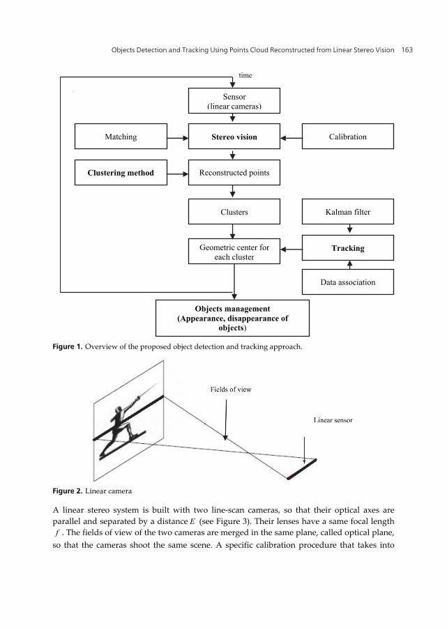
Objects Detection and Tracking Using Points Cloud Reconstructed from Linear Stereo Vision 163
Figure 1. Overview of the proposed object detection and tracking approach.
Figure 2. Linear camera
A linear stereo system is built with two line-scan cameras, so that their optical axes are parallel and separated by a distance E (see Figure 3). Their lenses have a same focal lengthf . The fields of view of the two cameras are merged in the same plane, called optical plane,
so that the cameras shoot the same scene. A specific calibration procedure that takes into
Sensor(linear cameras)
(
ikG
ikG
Stereo vision
Reconstructed points
Clusters
Geometric center for each cluster
Calibration Matching
Clustering method
Tracking
Data association
Kalman filter
Objects management(Appearance, disappearance of
objects)
time

Current Advancements in Stereo Vision 164
account the fact that the line-scan cameras cannot provide the vertical information is developed in [11].
Figure 3. Geometry of the linear stereoscope
3.1. Feature extraction
The first step in stereo vision is to extract from each image the primitives to be matched. In classic video images, one can extract different types of primitives. In the case of linear images, the choice is restricted as a result of the onedimensional nature of the profile of a linear image. The only possibility in this case is to search for edge points corresponding to the frontiers of different objects present in the image (see Figure 4).
Figure 4. Type of primitives with linear images
The low-level processing of a couple of two stereo linear images yields the features required in the correspondence phase. Edges appearing in these simple images, which are one-dimensional signals, are valuable candidates for matching because large local variations in the gray-level function correspond to the boundaries of objects being observed in a scene.
Stereoscopic axis
Optical plane f
E
Optical axis of the left camera
Optical axis of the right camera
Planar field of the left camera
Stereo vision sector
Planar field of the right camera

Objects Detection and Tracking Using Points Cloud Reconstructed from Linear Stereo Vision 165
Edge extraction is performed by means of the Deriche’s operator and a technique that selects pertinent local extrema by splitting the gradient magnitude signal into adjacent intervals where the sign of the operator response remains constant [10]. In each interval of constant sign, the maximum amplitude indicates the position of a unique edge associated to this interval when, and only when, this amplitude is greater than a low threshold value (see Figure 5).
Profile of a linear image
Local extrema selected
+ + + + ++
- - - --t
Insignificant extrema
t
Figure 5. Extraction of edge points
Applied to the left and right linear images, this edge extraction procedure yields to two lists of edges, where each edge is characterized by its position in the image, the amplitude and the sign of the response of Deriche's operator.
3.2. Stereo matching
The edge stereo matching task can be viewed as a constraint satisfaction problem where the objective is to highlight a solution for which the matches are as compatible as possible with respect to specific constraints. Our approach for solving the stereo correspondence problem is based on two types of constraints: local constraints (position and slope constraints) and global ones (uniqueness, smoothness and ordering constraints). The local constraints are used to discard impossible matches so as to consider only potentially acceptable pairs of edges as candidates. Applied to the possible matches in order to highlight the best ones, the global constraints are formulated in terms of an objective function, which is defined so that the best matches correspond to its minimum value. A Hopfield neural network is then used to map the optimization process [10].

Current Advancements in Stereo Vision 166
Once the matching process is achieved, a simple geometric triangulation allows obtaining for each matched edge pair a 2D point characterized by its horizontal position and depth. Line-scan cameras cannot provide the vertical information.
Let us define the base-line joining the perspective centers Ol and Or as the X-axis, and let Z-axis lie in the optical plane, parallel to the optical axes of the cameras, so that the origin of the X,Z coordinate system stands midway between the lens centers (see Figure 6). Let us consider a point ( , )P x zp p of coordinate px and pz in the optical plane. The image coordinates lx and rx represent the projections of the point P in the left and right imaging sensors, respectively. This pair of points is referred to as a corresponding pair. Using the pinhole lens model, the coordinates of the point P in the optical plane can be found as:
E.fZ =p d (1)
x .Z x .ZE Ep r plX = - = +p f 2 f 2
(2)
where f is the focal length of the lenses, E is the base-line width and d =xl xr is the disparity between the left and right projections of the point P on the two sensors.
Figure 6. Pinhole model
f
Z
X
xr xl
Or Ol O
zP
E
P(xP,zP)
xP
Left sensor Right sensor

Objects Detection and Tracking Using Points Cloud Reconstructed from Linear Stereo Vision 167
4. Objects detection
Objects detection is an important and yet challenging vision task. It is a critical part in many applications such as image search and scene understanding. It is still an open problem due to the complexity of object classes and images. In this chapter, we are interested in detecting objects using a cloud of points reconstructed from linear stereovision. The proposed method is based on an unsupervised classification approach using spectral clustering.
4.1. Spectral clustering
Let us consider a list of points reconstructed from a pair of linear images. The objective is to cluster the points so that each cluster corresponds to an object of the scene. The difficulty is that no a priori knowledge on the distribution of the reconstructed points is available. Furthermore, the number of the clusters is unknown. Since classical deterministic classification techniques are not adapted, we propose to use a spectral learning based clustering approach [13, 14]. This approach allows also avoiding the problem of local minima inherent to the most part of classification methods. The principle of this approach is to perform spectral decomposition of a similarity matrix, constructed form the data to be clustered. The decomposition consists in extracting the eigenvectors of a transition matrix, calculated from the similarity matrix. The analysis of these eigenvectors can detect the different structures in the data to classify [15-17].
4.2. Spectral clustering algorithm
Consider a set of n points ,......1L P Pn to be segmented in order to extract the clusters that correspond to the objects observed in the scene. A point iP is characterized by its horizontal position and depth that are extracted from the linear stereovision process. The spectral clustering algorithm can be summarized as follows:
1. First, one must form a matrix A in n nR . Called the affinity matrix, this matrix represents the similarity between the point pairs. In our case, more the distance between two points is small more is high their similarity. Hence, the objective is to affect to the same cluster the points that are close each other in their representation space. The similarity can be represented by different forms: Cosine, Gaussian, or Fuzzy function [14]. In this paper, the Gaussian representation which generally the more used in the literature is adopted. The Gaussian similarity matrix is defined by equation (3)
2d ,
A expij 2P Pi j
(3)
for i # j and 0Aii , where ,d P Pi j is a distance function, which is often taken as the Euclidean distance between the points Pi and Pj , and σ is a scaling parameter which is further discussed in the next section.

Current Advancements in Stereo Vision 168
2. Define a diagonal matrix D as D Aii ijj .
3. Normalize the affinity matrix A to obtain a transition matrix N . We use the following normalization form (see Table 1):
-1 -12 2N D AD (4)
4. Form the matrix 1[ ,......., ]kX X X in *n kR , where X ,......., X1 k are the k eigenvectors of the matrix N , corresponding to the k significant eigenvalues 1,......, k .
5. Normalize the lines of the matrix X to have a unit module. 6. Consider each line of the matrix X as a point in kR , and perform a classification using
K-means algorithm with k classes. 7. Run M times the K-means algorithm and conserve the optimal partition for which the
intra-class inertia is minimal, where M is the number of possible partitions. 8. Assign the point Pi to the class Cj if and only if the line Xi of the matrix X has been
assigned to the class Cj .
Table 1 gathers different types of normalization forms applied to the affinity matrix.
Normalization f(A, D)
Division -1N = D A Symmetric division
1 1- -2 2N = D AD Nothing N = A
normalized additive
(A+ d I - D)maxN =dmax
d = max(D )= max( A )max ii iji i j
Table 1. Different forms of the normalization function
The spectral clustering requires the adjustment of two parameters. The first one is the scaling parameter , which is used in the expression of the affinity matrix A . The second one is the number of classes k that corresponds to the k significant eigenvalues of the transition matrix N . The goal is to estimate automatically these two parameters, in order to make the clustering process as a nonparametric and unsupervised classification method.
4.3. Estimation of the scaling parameter
As expressed in equation (3), the performance of spectral clustering depends on the scaling parameter . Thus, choosing optimally the value of this parameter is an important issue. In [17], the authors suggested choosing automatically by running their clustering algorithm repeatedly for a number of values of and selecting the one providing less distorted

Objects Detection and Tracking Using Points Cloud Reconstructed from Linear Stereo Vision 169
clusters of the rows of the matrix X constructed in step 4 of the clustering algorithm. In [19], the authors propose two selection strategies, manual and automatic. The first one relies on the distance histogram and helps finding a good global value for the parameter . The second strategy sets automatically to an individually different value for each point, thus resulting in an asymmetric affinity matrix. This selection strategy was originally motivated by no homogeneously dispersed clusters, but it provides also a very robust way for selecting in homogeneous cases.
In our case, we adopted the selection strategy proposed in [17] for its simplicity. For that, different values for 2 are taken to select the value that provides less distorted clusters of the row of the matrix X .
4.4. Estimation of the number of clusters k
The evaluation of the parameter k can be performed by analyzing the eigenvalues i or the eigenvectors Xi of the matrix N [19]. In this work, we adopted an eigenvalues analysis. Theoretically, this analysis consists in considering the eigenvalues with a value equal to 1. In practice, significant eigenvalues have to be chosen by applying a thresholding procedure, i.e., eigenvalues that exceed a threshold are retained. We have chosen several forms of thresholding. One can consider also the difference between successive eigenvalues. The disadvantage of this strategy is that the jump between two successive eigenvalues can be big or small [20]. We tested this strategy in order to determine an empirical relationship. After various tests, we found that thresholding analysis gives the best results with a threshold m , which is set to the average of the eigenvalues.
5. Objects tracking
Objects tracking in a sequence of images is a basic problem, but important in many computer vision applications. It consists in reconstructing the trajectory of objects along the sequence. This problem is inherently difficult, especially when unstructured forms are considered for tracking. It is also very difficult to build a dynamic model in advance, without a priori knowledge of objects motion.
5.1. Modeling
In this work, we are interested in tracking objects, where each object is represented by a cluster of points. We recall that the clusters are obtained by the spectral clustering algorithm described in section 4.2. To model moving objects, we consider the hypothesis that the displacement of an object, represented by a cluster of points, is modeled by the displacement of the geometric center of the points. We can therefore apply the fundamental principle of point dynamic to express the following equations:
. ..1 2( ) ( - ) . . .
2x t x t dt x dt x dt (5)

Current Advancements in Stereo Vision 170
. ..1 2( ) ( - ) . . .
2z t z t dt z dt z dt (5)
Where x is the horizontal position and z is the depth of the geometric center of a cluster representing an object.
The most popular approach used for tracking mobile objects is based on Bayesian filters, especially Kalman Filters (KF) under a Gaussian noise assumption. KF is a tool for estimating object’s state and smoothing its changes. In our case, KF is used with the Discrete White Noise Acceleration Model (DWNA) to describe object kinematics and process noise [21].
5.2. Kalman filter
Kalman filter is a set of mathematical equations that provides an efficient computational (recursive) means to estimate the state of a process, in a way that it minimizes the mean of the squared error. The filter is very powerful in several aspects: it supports estimations of past, present, and even future states, and it can do so even when the precise nature of the modeled system is unknown. Kalman filter addresses the general problem of estimating the state
nS R of a discrete-time controlled process governed by a linear stochastic difference equation [22]. The discrete-time state equation with sampling period T is expressed as follows:
( 1) ( ) ( 1)S k F S k W k (7)
In this work, the state ( )S k is composed with the position and velocity of the geometric center of a cluster representing an object:
( ) [ ] tS k x v z vx z
The State Transition Matrix F is given by:
1 0 00 1 0 00 0 10 0 0 1
T
FT
The target acceleration is modeled as a white noise ( )W k . The measurement model mY R is given by:
( ) ( ) ( )Y k H S k V k (8)
where H is the observation model:
10000010
H

Objects Detection and Tracking Using Points Cloud Reconstructed from Linear Stereo Vision 171
The random variables ( )W k and ( )V k represent the process and measurement noises, respectively. They are assumed to be independent, white, and with normal probability distributions:
( ) ~ (0, )( ) ~ (0, )
P W N QP V N R
(9)
In practice, the process noise covariance Q and measurement noise covariance R matrices might change with each time step or measurement. In this paper, we assume that they are constant.
Kalman filter can be written as a single equation. However, it is most often conceptualized as two distinct phases: Prediction phase and updating phase (see Figure 7). The prediction phase uses the state estimated from the previous time step to produce an estimate of the state at the current time step. The predicted state estimate is known as the a priori state estimate, because although it is an estimate of the state at the current time step, it does not include observation information from the current time step. In the updating phase, the current a priori prediction is combined with the current observation information to refine the state estimate. This improved estimate is known as the a posteriori state estimate.
Figure 7. Stages of Kalman Filter
For multiple tracking, the problem of data association must be handled. The proposed data association algorithm is presented in the section 5.4.
5.3. Kalman filter algorithm
Initialisation
i i i i iS (k - 1),P (k - 1),R = Q = P (k - 1)apos apos apos
Prediction
i iS (k)= F S (k - 1)apr apos (10)

Current Advancements in Stereo Vision 172
i i T iP (k)= F P (k - 1) F +Qapr apos (11)
Updating
i iY = H Sapr apr (12)
i iRes(k)= Y (k) - H Sapr (13)
i T iC(k)= H P (k) H + Rapr (14)
i i T -1K (k)= P (k) H (C(k))apr (15)
i i i iS (k)= S (k)+ K (k) Res (k)apos apr (16)
i i iP (k)= (1 - K (k) H) Papos apr (17)
where:
aprS is the a priori state estimate;
aposP is the a priori estimate error covariance
aposS is the a posteriori state estimate;
aposP is the a posteriori estimate error covariance
aprY is the predicted measurement ; Res is the measurement innovation, or the residual.
C is the innovation covariance; K is the filter gain
Y is the sensor measurement; i corresponds to the thi geometric center to track.
5.4. Data association
Once the prediction step is achieved, one must perform data association between predicted objects and observed ones from measurements provided by the sensor. Data association is a problem of great importance part for multiple target tracking applications. In this section, we describe a method of data association for tracking multiple objects where the number of objects is unknown and varies during tracking.
In the literature, there are many data association algorithms such as Nearest-Neighbour (NN), Probabilistic Data Association (PDA), Joint PDA (JPDA) and multiple hypotheses tracking (MHT) [23, 24]. In this paper, we used the Nearest Neighbour (NN) method, which is simple to implement: for each new set of observations, the goal is to find the most Mahalanobis distance based likely association between an observation and an existing track, otherwise between a new observation and the new track assumption. In our case, we are interesting to track the geometric centers of the obtained clusters representing the objects in the scene.

Objects Detection and Tracking Using Points Cloud Reconstructed from Linear Stereo Vision 173
Mahalanobis distance is defined by:
12 1( , ) ( ) ( )2
Td Y Y Y Y C Y Ym apr apr apr (18)
where:
C is the covariance matrix of Res , which is the measurement innovation (see Equation 14). Yapr is the predicted measurement (see Equation 12).
Y is the measurement provided by the sensor.
The Mahalanobis distance is a statistical distance that takes into account the covariance and correlation of the elements of the state vector, and is appropriate to solve the data association problem. In our case, the covariance and correlation are determined between the measurements provided by the sensor and the predicted measurement given by Kalman filter.
The first step for data association is to define a search area for candidate points to the association. The size of searching area, which must be defined for each geometric center representing an object, depends on the movement of the object. Uncertainty about the movement defines the search area taken as a circle. Let iGk be the searching circle of the predicted object i at time k . The ray of this searching circle is defined by equation (19).
iray(G )= Δv(x,z)k (19)
where Δv(x,z) is the difference between the velocities at times k and k - 1 .
The data association process is first applied considering the horizontal position x . The results are then validated by the data association process with the depth z .
5.5. Temporal constraint
Tracking requires information about the past of the objects. Indeed, when an object appears for the first time, one cannot decide reliably if the object is real or corresponds to a wrong detection considering that the sensor can generate false detection (i.e the observation does not match any known object). To make objects tracking more robust, an object must be detected and tracked during a sufficient long period in order to assess objects appearance and disappearance. This temporal constraint will allow ignoring objects generated erroneously from the stereo matching process. The temporal constraint consists in associating a minimum lifetime to each object [12]. In our case, we set the minimum lifetime to 5 successive detections: when an object is not detected during 5 successive frames, we estimate that it disappears.

Current Advancements in Stereo Vision 174
5.6. Fusion of objects
The spectral clustering may sometimes produce two or more distinct objects that represent in reality a single object. Indeed, points representing the same object may be segmented onto two or more clusters of points. To resolve this problem, we propose a clusters fusion technique based on a clusters overlapping strategy. The fusion technique consists in determining an overlapping coefficient, defined as follows:
dist(o ,o )i jT =c r + ri j
(20)
with:
oi and jo are respectively the geometric centers of the clusters i and j, candidates for a
possible fusion. dist(o ,o )i j is the Euclidean distance between the geometric centers oi and jo .
ri and rj are respectively the rays of the search areas of the two tracks i and j. The rays
ir and rj are determined in the data association step. The ray ri is calculated as the
difference between the estimated (KF-based) and real (observation-based) positions. When the overlapping coefficient Tc is greater than a threshold, the considered clusters are merged. In this work, the overlapping threshold is set experimentally to 0.5.
6. Results and discussion
Our approach is tested and evaluated for obstacle detection and tracking in front a vehicle. The line-scan cameras based stereo set-up (see Figure 8) is installed on top of a car for periodically acquiring stereo pairs of linear images as the car travels (see Figures 9 and 10) [11, 12]. The tilt angle is adjusted so that the optical plane intersects the pavement at a given distance Dmax in front of the car. The cameras have a sensor width of 22.1 mm, a focal length of 100 mm and deliver images with resolution of 1728 pixels. Within the stereo setup, the cameras are separated by a distance E = 1m .
Figure 11 represents a stereo sequence, in which the linear images are represented as horizontal lines, time running from top to bottom. The pedestrian travels in front of the car according to the trajectory shown in (Figure 12). On the images of the stereo sequence, we can clearly see the white lines of the pavement. The shadow of a car, located out of the vision field of the stereoscope, is visible on the right of the images as a black area.
The disparities of all matched edges are used to compute the positions and distances of the edges of the objects seen in the stereo vision sector. The results are shown in (Figure 13), in which the distances are represented in grey levels, the darker the closer, whereas positions are represented along the horizontal axis. As in (Figure 11), time runs from top to bottom.

Objects Detection and Tracking Using Points Cloud Reconstructed from Linear Stereo Vision 175
Figure 8. Linear cameras composing the stereoscope.
Figure 9. Stereo set-up, side view
Figure 10. Stereo set-up, top view
The clustering stage is performed on the reconstructed points for each pair of stereo linear images. The tracking process is applied to the geometric center of the obtained clusters representing the objects in the scene. The results are illustrated in (Figures 14, 15 and 16), time runs from top to bottom.
Optical plane
E
Stereo vision sector
Planar field of the right camera
Planar field of the left camera

Current Advancements in Stereo Vision 176
Figure 11. Stereo sequence (pedestrian) a- Left sequence b-Right sequence
The detected and tracked objects are labelled as follows: white lines in blue (with crucifix), shadow transition in black (with crucifix), and the pedestrian in purple (with star), red (with square) and black (with square). One can see that all the objects are detected and tracked correctly. Some errors are identified, especially when occlusions occur at the end of the sequence, i.e., when the pedestrian hides one of the white lines to the left or right camera. These errors are caused by matching the edges of the white line, seen by one of the cameras, with those representing the pedestrian. These errors effect the clustering task and hence the tracking process. Some of these errors could be removed by exploiting the tracking results in the matching procedure. As mentioned before, the clustering process may provide two or more clusters for the same object. This situation occurs when the number of clusters is over estimated by the spectral analysis. In (Figure 14), one can see that this situation occurs for the detection of the pedestrian. To solve this problem, the proposed clusters fusion strategy is applied. The results are illustrated in (Figure 15) in which all of the clusters representing the pedestrian are merged.
Figure 12. Trajectory of the pedestrian during the sequence
(a) (b)

Objects Detection and Tracking Using Points Cloud Reconstructed from Linear Stereo Vision 177
Figure 16 shows the evolution of the detected and tracked objects according the horizontal position x and depth z . In this figure, one can see that the position and depth of the white lines (crucifix in blue) and shadow transition (crucifix in black) is stable. The figure illustrates also the reconstructed trajectory of the pedestrian (stars in purple, and squares in red and black).
Figure 13. Image reconstruction of the stereo sequence pedestrian
Figure 14. Objects detection and tracking (plot of the horizontal position x when time runs from top to the bottom)

Current Advancements in Stereo Vision 178
Figure 15. Objects detection and tracking with the data fusion strategy
Figure 16. Objects detection and tracking with the data fusion strategy (plot of the horizontal position x and depth z)
7. Conclusion
A method for detecting and tracking objects using linear stereo vision is presented. After reconstructing 3D points from the matching edge points extracted from stereo linear images, a clustering algorithm based on a spectral analysis is proposed to extract clusters of points where each cluster represents an object of the observed scene. The tracking process is achieved using Kalman filter algorithm and nearest neighbour data association. A fusion strategy is also proposed to resolve the problem of multiple clusters that represent a same object. The proposed method is tested with real data in the context of objects detection and tracking in front of a vehicle.

Objects Detection and Tracking Using Points Cloud Reconstructed from Linear Stereo Vision 179
Author details
Safaa Moqqaddem Systems and Transportation Laboratory, University of Technology of Belfort-Montbéliard, Belfort, France LASTID Laboratory, Ibn Tofail University of Kénitra, Morocco
Y. Ruichek Systems and Transportation Laboratory, University of Technology of Belfort-Montbéliard, Belfort, France
R. Touahni and A. Sbihi LASTID Laboratory, Ibn Tofail University of Kénitra, Morocco
Acknowledgement
The work presented in this paper is a part of a project aiming to develop advanced driving aid systems. The authors would like to thank the CPER, STIC and Volubilis programs for their support.
8. References
[1] Banks, Jasmine Elizabeth, Bennamoun, Mohammed, Kubik, Kurt, & Corke, Peter . "A taxonomy of image matching techniques for stereo vision". Queensland University of Technology, Brisbane. 1997
[2] F.Mrabti, H.Seridi. "Comparaison de méthodes de classification réseau RBF, MLP et RVFLNN". Damascus University Journal Vol. (25) - No. (2) 2009.
[3] Teuvo Kohonen. "Self-organizing maps". Springer-Verlag New York, Inc., Secaucus, NJ, USA, 1997.
[4] H. Frigui et R. Krishnapuram. "Clustering by competitive agglomeration". Pattern Recognition Journal, 30(7) :1109–1119, 1997.
[5] Bertrand Le Saux et Nozha Boujemaa. " Image database clustering with svm-based class personalization". Conference on Storage and Retrieval Methods and Applications for Multimedia / Electronic Imaging symposium (SPIE ’04), San Jose, CA, USA, Janvier 2004.
[6] Daniel Boley. " Principal direction divisive partitioning". Data Min. Knowl. Discov., 2(4) :325–344, 1998.
[7] O.Zammit, X.Descombes et J.Zerubia. "Apprentissage non supervisé des SVM par un algorithme des K-moyennes entropique pour la détection de zones brûlées". Colloque GRETSI Groupe d’Etudes du Traitement du Signal et des Images, 11-14 septembre 2007, Troyes.
[8] G. Palubinkas, X. Descombes et F. Kruggel. "An un- supervised clustering method using the entropy minimization". IEEE International Conference on Pattern Recognition, Brisbane, Australie, 1998.

Current Advancements in Stereo Vision 180
[9] Sergio Nogueira, Yassine Ruichek and François Charpillet " A Self Navigation Technique using Stereovision Analysis ", 295-306p, stereo vision. Edited by Dr. Asim Bhatti.
[10] Ruichek, Y., Hariti, M., and Issa, H., "Global techniques for edge based stereo matching", Scene Reconstruction Pose Estimation and Tracking, Rustam Stolkin (Ed.), I-Tech Education and Publishing, Austria, pp 383–410, 2007.
[11] Bruyelle, J. L, "Conception et réalisation d’un dispositif de prise de vue stéréoscopique linéaire– Application à la détection d’obstacles à l’avant des véhicules routiers", Phd thesis, Université des Sciences et Technologies de Lille, France 1994.
[12] Burie, J. C., Bruyelle, J. L., and Postaire, J. G., "Detecting and localising obstacles in front of a moving vehicle using linear stereo vision", Mathematical and Computer Modeling 22(4–7), 235–246, 1995.
[13] Kamvar, S. D., Klein, D., and Manning, C. D., "Spectral learning" Proc. International Joint Conference on Artificial Intelligence, 2003.
[14] Francis R. Bach and Michael I.Jordan." Learning Spectral Clustering". Report No.UCB/CSD-03-1249. June 2003.
[15] Lihi Zelnik-Manor and Pietro Perona, "Self-Tuning Spectral Clustering", Advances in Neural Information Processing Systems 17, pp 1601-1608, 2004.
[16] Weiss, Y., "Segmentation using eigenvectors: a unifying view", Proc. IEEE International Conference on Computer Vision, pp 975-982, 1999.
[17] Ng A. Y., Jordan, M. I., and Weiss, Y. "On spectral clustering: Analysis and an algorithm". Advances in Neural Information Processing Systems 14, Cambridge, MA. MIT Press, 2002.
[18] Verma D. and Meila M. "A comparison of spectral clustering algorithms", Technical report uw-cse-03-05-01, university of washington, 2003.
[19] Sanguinetti G., Laidler J. and Neil L. "Automatic determination of the number of clusters using spectral algorithms", In IEEE Machine Learning for Signal Processing 2005, 28-30 Sept 2005, Mystic, Connecticut, USA.
[20] Inderjit Dhillon, Yuqiang Guan, Brian Kulis, "Kernel k-means, Spectral Clustering and Normalized Cuts", KDD’04, August 22–25, Seattle, Washinton, USA, 2004.
[21] Bar-Shalom, Y., Li, X., and Kirubarajan, T., "Estimation with applications to tracking and navigation", Wiley, New York, chapter 6, 2001.
[22] Arnaud, E., "Méthodes de filtrage pour du suivi dans des séquences d'images - Application au suivi de points caractéristiques", Phd thesis, Université de Rennes I, France ,2004.
[23] Jaco Vermaak, Simon J. Godsill and Patrick Pérez. "Monte Carlo Filtering for Multi-Target Tracking and Data Association". DRAFT, September 22, 2004
[24] Coué, C., "Modèle bayésien pour l'analyse multimodale d'environnements dynamiques et encombrés : Application à l'assistance à la conduite en milieu urbain, " Phd thesis, Institutational Polytechnique de Grenoble, France, 2003.

Chapter 0
3D Probabilistic Occupancy Grid to RoboticMapping with Stereo Vision
Anderson A. S. Souza, Rosiery Maia and Luiz M. G. Gonçalves
Additional information is available at the end of the chapter
http://dx.doi.org/10.5772/49050
1. Introduction
Environment mapping is considered an essential skill for a mobile robot in order to actuallyreach autonomy [1]. The robotic mapping can be defined as the process of acquiring aspatial model of the environment through sensory information. The environment mapallows mobile robots to interact coherently with objects and people in this environment. Therobot can safely navigate, identify surrounding objects and have flexibility to dealing withunexpected situations. Without a map some important operations could be complex as thedetermination of objects position in the surroundings of the robot and the definition of thepath to be followed. These issues involve the importance of the mapping task be performedcorrectly, since the acquisition of inaccurate maps can lead to errors in the inference ofcorrect positioning of the robot, resulting in an imperfect implementation of these operations.Therefore there is a mutual dependence between inferring the exact localization of the robotand building an accurate map.
There are several researches done in robotics mapping proposing ways to represent a mappedenvironment, all of them concerned in dealing with high dimensional mapped environment.The work of Agelopoulu et al. [3] provides a good overview on articles published at thevery early period of research about mapping and it reports the several different ways ofrepresenting the environment, focusing on the main features of each approach. Thrun [1]proposes a classification of the ways of representing an environment mapped into two maincategories: metric and topological representations. The metric representations store geometricproperties of the environment, whereas the topological representations describe connectivitybetween different places. Within the metric representations, the occupancy grid stands out byproviding a relatively accurate reproduction of the mapped environment.
Robots can be used to map internal or external environments depending on the task typesupported by them. Lee et. al. [4], for example, uses a mobile robot equipped withsonar to build a features-based map. The robot finds points, lines and circles in theenvironment through processing of the information provided by sonar. Dealing with external
Chapter 9

2 Will-be-set-by-IN-TECH
environments, Guivant et. al. [5] has implemented a mobile vehicle to map an environmenttypical of a farm. The map built by the vehicle was composed of typical objects of theenvironment, as trees and stakes. However, the majority of the works dealing with the roboticsmapping theme do not discuss a generalist alternative to provide the mapping of both internaland external environments. The difficulty is in the detection of characteristics inherent inall kind of environments. It is well known that internal environments are more structured,so that the vast majority of them have common cues, for example, lines, nooks and corners.External terrain mapping depends on the objects that can be highlighted in them (transit cards,buildings, trees, and rocks, among others).
Several types of sensors can be used for carrying out the mapping. The most common aresonar, lasers and cameras. The sonar is attractive because of its low cost. Besides beingrelatively inexpensive they can be easily found in a commercial market. However, sonarpresents significant inaccuracies in the measurements acquired. Lasers are highly accurateand provide the acquisition of detailed maps but they are not attractive because of its highcost. Cameras are sensors that, at each day, are getting cheaper and they make possiblethe acquisition of a large amount of information surrounding the robot. For these reasons,cameras are playing an important role among the sensors used for robotic mapping.
This chapter proposes the mapping of internal and/or external environments through asystem of stereo cameras of low-cost with metric representation of the environmental in aprobabilistic occupancy grid. With the stereo vision system the robot can collect informationfrom different places with different types of obstacle, and it does not dependent on the type ofenvironment in which it is located or the type of features inside this place. The mappingalgorithm considers a probabilistic modeling for the vision system used by the robot, aswell as to its performed movements. With this, the 3D Probabilistic Occupancy Grid toRobotic Mapping with Stereo Vision generates results (maps) consistent with the informationobtained by the robot. To attest to the feasibility proposed by that research will be presentedpreliminary experiments performed.
The article is structured as follows: section 2 presents the problem of environment mappingwith robots. The section introduce the occupancy grid mapping. Section 3 contextualizesthe same problem with the use of visual sensors (cameras). In section 4 will be presentedthe proposed mapping with stereo vision and occupation grid representation. Section 5expose the preliminary results achieved with the mapping algorithm. Finally, the section 6brings the concluding remarks, directing to the next steps that will be given toward the fullimplementation of the system.
2. Robotic mapping
To better formalize the problem of robotic mapping, we need to establish some basicassumptions (or restrictions). The first hypothesis is that the robot has proprioceptive andexteroceptive sensors that allow collect data about yourself (position and orientation) andabout the environment. The second is that perception system must always provide the exactknowledge of the position and orientation of the robot relative to any coordinate system orframe of global fixed reference adopted.
With these assumptions, we can define the robotic mapping as the problem of building a spacemodel of the environment by the robotic computational system, based on data provided by
182 Current Advancements in Stereo Vision

3D Probabilistic Occupancy Grid to Robotic Mapping with Stereo Vision 3
the perception system. The Figure 1 illustrates the evolution of the process of building a map.In this illustration, x represents the robot pose (position and orientation), z represents thesensory measurements collected over time, and m represents the map being built iterativelyat each time interval.
xt
xt+1
xt-1
zt
zt+1
zt-1
m
Figure 1. Mapping process.
The hypothesis that the perception system has the exact knowledge of the robot positionand robot orientation relative to some global reference adopted is not always true. And inmost cases to get the exact position and orientation of the robot inside of your environmentis necessary to have a map. Here a conflict arises: to get a consistent map is required exactknowledge of the robot position and orientation, and for this, it is necessary an environmentmap. Note that there is a dependency between location (inferring the position and orientationof the robot in the environment) and mapping. To resolve this conflict some researchersextend the mapping problem to a simultaneous localization and mapping problem or simplySLAM [2].
From this point, we assume as true the hypothesis that the robot position and orientation areknown somehow. Then specifically we approach the mapping problem with known positionand known orientation, as proposed by Thrun [6]. It should be noted that even assumingthis assumption, the following challenges need to be overcome [1]: sensory inaccuracies,dimensionality of environment, data matching, dynamism of the environment and operatingstrategy. Then each of these challenges will be detailed.
2.1. Sensory uncertainties
The sensors used for robotic mapping are influenced by several sources of noise that causeerrors in his measurements. An important issue in the mapping environments is how todeal with the uncertainties and inaccuracies found in the data provided by these sensors.Inaccuracies can be caused due to many factors intrinsic to the type of device used. Inaddition, there are also the errors inherent in the robot movements within its environment,which can be caused by systemic factors, such as the uncertainties present in parametersthat are part kinematic modeling of the robot (for example, differences in the size of thewheels, erroneous measurement axes) and/or by non systematic factors as uncertainties fromunexpected situations (for example, collision with unexpected objects, wheel slip) [7].
The challenge occurs depending on the type of the noise in measurements, in the other words,to model the robotic mapping problem would be relatively easy if the noise in differentmeasurements was statistically independent. However, there is a statistical dependency that
1833D Probabilistic Occupancy Grid to Robotic Mapping with Stereo Vision

4 Will-be-set-by-IN-TECH
occurs because the errors inherent in the robot movements accumulate over time, and affecthow the sensory measurements are interpreted. To overcome this challenge, generally theerror sources are modeled or approximated by stochastic functions, allowing the sensory dataare handled properly during the mapping process. When these factors are disregarded, weare likely to witness the construction of inconsistent and inaccurate maps.
2.2. Dimensionality
Another challenge that arises in the mapping problem refers to the dimensionality of theenvironment to be mapped. Imagine an environment typically simple, such as a house withrooms, corridors and kitchen. If it is considered just a topological description of compartmentswill require a few variables to describe this environment. However, when the goal is to get richmaps in detail with two (2D) or three (3D) dimensions, the complexity to estimate this map islarger and, in addition, it is necessary to increase the space for storing its representation in thecomputer memory.
Furthermore, cannot forget the larger and more complex the environment, higher is theprobability of some kind of error in the robot movements, which can prejudice the qualityof built map.
2.3. Matching
During the mapping, normally a same object or obstacle in the environment is perceivedseveral times by the robot, in different moments. Therefore is desirable that this object shouldbe identified as mapped and must be distinguished from those not yet mapped. This problemis known as matching or data association.
The lack of data association in the mapping can generate inconsistencies and differencesin maps. An effective scheme of matching must make distinctions between spuriousmeasurements, new measurements and lost measurements together with a basic function toassociate the available map with the new measurements. A study of the techniques moreused to solve the matching problem can be found in the work of Wijesoma et al. [8], where arepresented the general idea of solutions and their respective original references.
A method widely used in matching is the Nearest Neighbor - NN [9]. This method associatesa map point to the nearest observation inside a region of validation, based on some distance,which is usually given by the Mahalonobis distance. This method is attractive because theimplementation is easy, however it gives poor results. Other robust methods of solving thematching problem can be checked in the literature, for example, the Joint Probabilistic DataAssociation (JPDA) [10], Joint Compatibility Branch and Bound (JCBB) [11], Multi HypothesesTracking (MHT) [12] and "lazy" data association method (a variant of MHT) [13].
2.4. Dynamism of the environment
Another challenge arises when the interest is in mapping dynamic environments or notstationary, such as offices where people travel constantly and manufactures where objects aretransported to different places. In these cases, the robotic system can consider such changesas inconsistent measurements taken at a given time. Think about the case where, in a givenmoment, a robot maps a table in your environment. Then, for some reason, this table is moved
184 Current Advancements in Stereo Vision

3D Probabilistic Occupancy Grid to Robotic Mapping with Stereo Vision 5
to another location at a later time, and this change of location, which should be changed alsoon a robot map, does not occur. With this, when the robot go through the place where thetable was previously may seem that the robot is in a new location not yet mapped, becausethe object that should be detected, it is not.
The vast majority of mapping algorithms considers that the process is running in staticenvironments, and this makes the mapping problem of dynamic environments be largelyunexplored. However, in recent years, several proposals have emerged to solve this problem.For example, Biswas et al. [14] proposes a mapping algorithm in the occupation grid calledRobot Object Mapping Algorithm - ROMA, able to model not stationary environments. Theapproach assumes that objects move slowly in the environment that can be considered staticin relation to time it takes to build a map in occupation grid. The proposed algorithm is ableto identify such moving objects, learn the model of them and determine their location at anytime. It also estimates the total number of distinct objects in the environment, making theapproach applicable to situations where not all objects not stationary are visible at all times.The changes in the environment are detected by a simple technique of differentiation of maps.
Wolf and colleague [15] propose an approach based on differentiation of maps, howeverthe differentiation is made between a map of occupancy grid with static parts, and a mapof occupancy grid with dynamic parts. The algorithm proposed is able to detect dynamicobjects in the environment and represent them on a map, even when they are outside therobot perceptual field. In a recent work, Baig and collaborators [16] propose the detectionof dynamic objects in the mapping process of external environments through the methodDetection And Tracking of Moving Objects (DATMO), from a vehicle equipped with laserand odometry.
2.5. Exploration strategy
During the mapping, the robotic system should choose certain paths to be followed. Giventhat the robot has some knowledge about the world, the central question is: where heshould move to get new information? This is done by operating strategy that determinesthe displacement that the robot should perform to meet all environment. At the process endwe have a visited environment map produced from the information provided by the robotsensors.
The choice and implementation of good operating strategy emerges as a fifth challenge for themapping problem. The exploration assumes that the robot position and robot orientation areprecisely known and focuses on bring the robot with efficiency throughout the environment tobuild the full map [17]. For this, the exploration strategy should consider a model of partiallybuilt environment, and from this to plan the movement action to be performed. Stachniss [17]describes the exploration strategy as a combination between the mapping and the planning.
It is important that it be considered the exploration strategy efficiency to avoid unnecessaryspending of time and energy. In addition, it is necessary that the robot is able to deal withunexpected situations that may arise during the operation and building of the map. A classictechnique of exploration is proposed by Yamauchi [18], which is based on the concept offrontiers (frontier-based exploration), that are regions forming limits between free spacesand unexplored spaces. When the robot moves toward a new frontier, it can understand
1853D Probabilistic Occupancy Grid to Robotic Mapping with Stereo Vision

6 Will-be-set-by-IN-TECH
unexplored spaces and add new information to your map. As result the mapped territoryexpands, retreating the limits between known regions and unknown regions. Leaving forsuccessive frontiers, the robot can constantly increase your knowledge of the world. SilvaJúnior [19], presents the idea of exploitation based on boundary value problems. Stachniss [17]presents a summary of several exploration techniques developed, comparing your proposalbased on coverage maps. In this strategy, the robot exploration actions are selected to providea reduction of uncertainties that affect the mapping.
2.6. Representation types
There are two main approaches to represent an environment using a mobile robot: therepresentation based in topological maps and the representation using metric maps [1].However, some authors prefer change this classification increasing another paradigm calledfeatures maps representation [20] [21]. This category, by storing metrics information of thenotable objects (features) of the robot environment, is treated here as a metric maps subset.The following are main peculiarities of these paradigms.
2.6.1. Topological maps
Topological maps are computationally represented by the graphs, which describes anarrangement of nodes (or vertices) connected by edges (links or arcs). Typically the graphsdescribe the free spaces for performing tasks. The nodes correspond to regions that havehomogeneous sensory information and the arcs reflect the connection between these regions.Intuitively the use of a graph to describe an environment is a great idea because graph isa compact structure for storage in memory of the robot computational system and can beused to model structures or enumerate processes, such as representation of cities connectedby roads, connections of the printed circuit board, and others. The main problem of thisrepresentation is the lack of a standard that define which structures are associated with thevertices and which relationships are described as links.
Still, the robot location using topological maps is abstract, this means that, there is no way todefine explicitly the robot position and robot orientation. However, it is possible to affirm inwhich graph node or in which environment regions it is.
The lack of standardization of which elements are considered nodes and edges of graphs iseasily seen. For example, Kuipers and colleague [22] uses map nodes to represent places,characterized by sensory data, and the edges represent paths between places, characterized bycontrol strategies. Thrun [23] uses a topological map obtained from a probabilistic occupancygrid partitioned into regions (nodes) separated by close passages (edges). In a recent work[24], the definitions of nodes and edges are made from a topology extraction method basedon Generalized Voronoi Diagram, that make the skeletonisation of the images provided by alaser, to produce appropriate topological information.
2.6.2. Metric maps
The metric representation or metric maps reproduce, with a certain accuracy degree, thegeometry of the environment in which the robot is inserted. Objects such as walls,obstacles and passages are easily identified in this approach, since the map maintains a good
186 Current Advancements in Stereo Vision

3D Probabilistic Occupancy Grid to Robotic Mapping with Stereo Vision 7
topographic relationship with the real world. The metric maps are represented by occupancygrids and features maps.
• Feature-based maps
The features maps store information of important elements founded in environment specificlocations (features). A feature can be understood as "something" easily notable inside theenvironment such as corners and edges. In images, special properties of the some parts(such as a circle, a line, or a region with particular texture) are usually identified. Lee andcolleagues [4] use a robot equipped with a sonar belt to build a features map with lines,points and circular objects. These features are differentiated according with the sonar readingsprocessing.
This does not impede others objects, such as doors, lights, trees, buildings, towers etc, are alsoused as notable features to be stored in a map. In the work of Guivant [5], for example, amobile vehicle gives the map of the typical and external environment of a farm, identifyingtrees as features to be stored in a map.
This map type usually stores geometric information of the chosen features and Detected, asfor example, cartesian coordinates or polar coordinates of features relatives to some fixedreference. Santana and Medeiros [7] use floor lines of internal environments as interestingfeatures to be detected. The map was built with the polar coordinates of the straightobtained from imaging by Hough transform. A great advantage of this map type is have acompact representation if compared to occupancy grid representations. However, it also hasdisadvantages, and the main one is the dependence of a pre-defined procedure to detect andextract environment features [17].
• Occupancy Grid
The representation using occupancy grid was initially proposed in 1987 and formalizedin 1989 by Alberto Elfes [25][26]. With this representation, the continuous spaces of theenvironment are discretized, so that the environment is being represented in the configurationof a grid or multi-dimensional matrix (2D or 3D). Each element of the matrix, also called cell,represents a environment location that can be occupied, empty or unexplored.
The occupancy grid representation initially was proposed to map environments in a 2Dgrid, however, after Elfes [25], Moravec [27] expanded this representation to a 3D discreteconfiguration innovating also the sensor type used for the construction of the map. UnlikeElfes who employed sonar in his experiments, Moravec used a stereo vision system in theconstruction of a 3D map. In addition, Moravec also proposed a new approach to indicatethe possibility of cell occupancy based on evidence theory of Dempster-Shafer, also differingfrom the Bayesian probabilistic approach proposed by Elfes. The 3D grid presented was calledevidence grid and each cell stores a value that indicates the evidence of occupation.
Another approach of grid representation was presented in the work of Oriolo et al. [28].In this work, the authors show that it is possible formulate and solve perception problemsand planning problems dealing with uncertainties using the set theory (fuzzy logic). Thebuilt map by this technique is defined as a fuzzy set, in which each point is associated toa real number that quantifies the possibility of the map pertain to an obstacle. The mainadvantage is the possibility of using several types of fuzzy operators to model uncertaintyand aggregate information from multiple sources. Ribo and Pinz [29] present a comparative
1873D Probabilistic Occupancy Grid to Robotic Mapping with Stereo Vision

8 Will-be-set-by-IN-TECH
study between the three approaches mentioned, showing their models to the range sensorsand checking the treatment of the uncertainties presents in the measurements. However, thecited work is restricted to experiments with robots equipped with sonar inserted in typicaloffice environments.
Other variations of these approaches can be seen in the literature. For example, Konolige [30]proposes a method that is a mathematical refinement of the mapping method presented byElfes [25], named MUltiple Representation Independent Evidence Log - MURIEL, aimingto control the intrinsic problems of the sonar, such as reflection multiples and redundantreadings. Borenstein and Koren [31] presents a method based on histograms. In this method,the main goal is to reduce the computational cost intrinsic to representation based occupancygrids. Another variation can be checked on work Yguel et al. [32]. This work reports the issuesof representation and data storage by large maps and, for this, proposes a form of occupancygrid representation based on wavelets: Wavelet Occupancy Grids.
Some changes of the default algorithm presented by Elfes [25] are proposals aiming to improvethe quality of built maps, considering computational cost of processing and storage [13],uncertainty treatment [33] and sensors modeling [34]. There are several recent examples inthe literature that attest the utility of the representation by occupancy grid in SLAM [36] [38],with applications like surveillance [30] [37], exploration [39], rescue [40], and others tasks.
3. Occupancy grid mapping
The models based on occupancy grid proposed by Elfes [26] is one of the most used metricapproaches. The environment is represented as a regular grid of cells, where the value of eachcell encodes its state that can be free, occupied, or not mapped (undefined). The occupancyvalue of a cell is determined using a probabilistic approach that has as input estimateddistances to objects calculated from data given by the sensors. Through a bayesian approach,it is possible to update the cell values at every time that a measure is performed. Note thata subset of the whole grid is updated each time. The resulting model can be used directlyas a map of the environment in navigation tasks as path planning, obstacle avoidance, andpose estimation. Figure 2 ilustrates the representation of a depth sensor measure in a 2Doccupancy grid. Grey cells have unknown occupancy values, white cells are free and blackcells are occupied. The main advantages of this method are: it is easy to construct and it canbe as accurate as necessary.
Figure 2. Occupancy grid representation in 2D. All cells of the grid are initialized with gray colormeaning that the occupancy value is not known at start. From the readings inside the field of view of thesonar, white cells (free) and black cells (occupied) can be determined.
The construction of a map based on occupancy grid involves the determination of theoccupancy probability of each cell. Let us assume that the occupancy probabilities ofneighboring cells are decoupled, that is, the probability that a cell is occupied does not affect
188 Current Advancements in Stereo Vision

3D Probabilistic Occupancy Grid to Robotic Mapping with Stereo Vision 9
the estimation of probability occupancy values for its neighboring cells. Besides this is not anideal assumption specifically in the case of cells representing the same object it turns easier theimplementation of the mapping algorithm without a substantial increasing in the measurederror. With this assumption, the probability of occupation of a map M can be factored into theproduct of the occupancy probability of each cell mn individually according to Equation 1.
P(M|x1:t, z1:t) = ∏n
p(mn|x1:t, z1:t) (1)
The construction of the map M depends on the history of robot localizations x1:t and onthe sensors readings z1:t performed in each localization. Updating the map is a processof repeating these readings, which can be performed from other locations with otherorientations. In practice, only cells currently inside the field of view of the sensors are tobe updated. The occupancy value of a cell mn is calculated by Equation 2.
p(mn |x1:t, z1:t) = 1 − 11 − elt,n
(2)
with
lt,n = lt−1,n + logp(mn|xt, zt)
1 − p(mn)− log
1 − p(mn |xt, zt)
p(mn)(3)
p(mn) is the occupancy value of the cell mn previously to any measurement that can beattributed according to the obstacles density in the environment. The probability p(mn|xt, zt)specifies the occupancy probability of cell mn conditioned to the sensor reading zt in the timet and depends on the sensor used, and is named inverse sensor model. More details of thestandard algorithm for occupancy grid can be found in the work of Thrun [34].
4. Mapping with stereo vision
4.1. Stereo vision
The term stereo vision is generally used in the literature to designate problems where itis necessary to recover real measures of points in a 3D scene from measures performed intheir corresponding pixels in two or more images taken from different viewpoints. Thedetermination of the 3D structure of a scene using stereo vision is a well known problem [41].Formally, a stereo algorithm should solve two problems: the matching (pixel correspondence)and the consequent 3D geometry reconstruction.
The matching problem involves the determination of pairs of pixels, one pixel from eachimage in each stereo pair, corresponding to the points in the scene that have been projectedto the pixels. That is, given a pixel x in the first image, the matching problem is solved bydetermining its corresponding pixel x′ in the second image, for all pixels in the first one. Inprinciple, a search strategy has to be adopted to find the correspondences. Several solutionsare proposed generally using restrictions to facilitate the matching. The epipolar geometry isone of these, that makes narrower the search space [41].
By using this restriction, given a pixel in the one image, the search for the corresponding pixelin the other image can be performed in a line thus substantially decreasing the search space(from 2D to 1D). In general, the result of the matching phase is a disparity map that has, for
1893D Probabilistic Occupancy Grid to Robotic Mapping with Stereo Vision

10 Will-be-set-by-IN-TECH
all corresponding pixels determined, the displacement in images coordinates of each matchedpixel in the second image.
The reconstruction of 3D geometry relates to the determination of the scene 3D structures.The 3D position of a point P in space can be calculated by knowing the disparity betweenpositions (in image coordinate system) of the corresponding pair of pixels x and x′ givenby the disparity map and by knowing the geometry of the stereo vision system. The lastis specified in two matrices: M (named external) and M′ (internal), which are previouslydetermined. The positions of pixels are used in the matching phase to calculated the disparitymap, which is then used directly in the process.
In order to better understand the stereo reconstruction problem, let us assume the systemgeometry shown in Figure 3. The system has two cameras with projection centers O and O′,respectively. The optical axes are perfectly parallel to each other and the two camera imagesare in the same plane (coplanar). The focal distance f is the distance from each projectioncenter to each image plane, assumed to be the same for both cameras. The baseline b is thedistance between the projection centers. The values of b and f are known a priori by usingsome camera calibration procedure [41].
(x , y )0 0
P
b
(x’, y’)
(x, y)
f
f
z
opticalaxis
opticalaxis
image frame
image frame
O’
O
(x y ’)0 0’,
Figure 3. Stereo geometry of a coplanar camera system.
In Figure 3, (x′o, y′o) and (xo , yo) are the coordinates of the pixels in each image center, that is,in the intersection of the optical axes and the image planes. A point P in the scene is projectedin the pixels (x′, y′) (left) and (x, y) (right) in the images. The distance zc of the camera systemto the point P can be calculated by Equation 4, in camera frame reference:
zc = f .bd
(4)
where b is the baseline as said above and d is the disparity between the corresponding pixels,given by d = x′ − x. Note that there is no disparity in y coordinate because the axes are
190 Current Advancements in Stereo Vision

3D Probabilistic Occupancy Grid to Robotic Mapping with Stereo Vision 11
parallel. From Equation 3, we can observe that zc is inversely proportional to d. In practicalsituations, d is limited considering a maximum and minimum distance of the system to thescene. These distances are empirically defined considering the scene. The other coordinatesof point Pc = (xc, yc, zc) in relation to the stereo system can be calculated by using Equations 5and 6.
xc = zc.(x − x0)
f(5)
yc = zc.(y − y0)
f(6)
The coordinates of a point in the camera coordinate system Pc can be transformed to worldframe. To do that, one just has to know the rotation matrix and translation vector that mapthe camera to world frame, and use Equation 7.
Pw = RT.Pc + T (7)
Parameters b, f , (x′o , y′o) e (xo , yo) are determined through a previous calibration of the stereosystem. we remark that even if the system does not follow the restrictions depicted in Figure3, it is possible to derive a general mathematical model for the problem. In this case, it wouldbe more complex to recover the 3D geometry. Besides, in the calibration process it is alsopossible to diminish or eliminate errors caused by lens distortions and illumination.
Stereo matching The stereo matching should determine, for all pixels in one image, the pixelsthat are their homologous in the other image. That is, to determine all pairs of pixels, one pixelfrom each image, that correspond to the projections of points in the scene. Once determinedthe matching, disparity d can be calculated as the difference between the coordinates of thecorresponding pixels in each image and the depth for all points in the scene can be calculatedby using triangle similarity. So determination of matching for all pixels is a fundamental step.In fact, due to occlusions and image errors, we get not completely dense matchings.
Between the several methods used for matching and disparity map calculation, in this workwe performed experiments with the two suggested in the work of Scharstein and Szeliski [42]:the block-matching and the graph-cuts. The block-matching determines the correspondencefor pairs of pixels with characteristics that are well discernible. Basically, this methodgives as result a disparity map in four main steps. The first is a previous filtering of theimages to normalize brightness and texture enhancement. The second step is the search forcorrespondences using the epipolar constraint. This step performs the summation of absolutedifferences between windows of the same size of both images to find the matching. As thethird step, a posterior filtering is performed in order to eliminate false matchings. In thefourth step, the disparity map is calculated for the trustable pixels. This method is consideredfast, in fact, its computational complexity depends only on the image size.
The graph-cuts algorithm treats the best matching problem as a problem of energyminimization, including two energy terms. The smoothness energy (SE) measures thesmoothness of disparity between neighboring pixels, which should be as smooth as possible.The second term is data energy (ED) that measures how divergent are corresponding pixelswith basis on assumed disparity. A weighted graph is constructed with vertices representingthe image pixels. The labels (or terminals) are all the possible disparities (or all discrete valuesin the interval of disparity variation). The edge weights correspond to the energy terms abovedefined. The graph cuts technique is used to approximate the optimal solution, that computes
1913D Probabilistic Occupancy Grid to Robotic Mapping with Stereo Vision

12 Will-be-set-by-IN-TECH
corresponding disparity values (each edge of the graph) to each pixel (vertex of the graph)[43].
4.2. Modeling probabilistic mapping with stereo disparity
The acquisition and manipulation of images produces a uncertainty Δd for the error in thecoordinates of a pixel. This causes an error factor Δzc in the estimation of the coordinate zccalculated from the disparity map, named depth resolution, which is given by Equation 8.
Δzc =z2
cb. f
.Δd (8)
In order to construct the environment model using occupancy grid, it is necessary to modelthe used sensor generally named the inverse measurement model. We adopt a modeling thatis similar to the one depicted by Andert [44], however we propose to incorporate the errorsinherent to robot motion in the calculation of the probability of occupation of a cell. Withthis modification, we get a map that is more coherent with the sensory data provided by therobot. We can guarantee a limit for the maximum error found in the map. This is extremelyimportant in the treatment of uncertainties encountered in the scene.
The inverse model transform the data provided by the sensors in the information contained inthe map. In our case, a distance measured from a specific point in the environment indicatesthe probability that part of the grid is occupied or free. Distance is calculated directly fromdisparity. In this way, it is possible to map each point of the space seen by the robot visionsystem with a valid disparity value into the possible values of elements of the occupancy grid.
In the measurement model, each point of the disparity map can act as a distance sensormeasured along the ray defined by the world coordinates of the pixel (in the image plane)and the projection center of the camera. The point in the image plane is given in cameracoordinates by Pc = (xc, yc, zc) and the distance of the camera to Pc is calculated by Equation 9with a sensorial uncertainty given by Equation 10.
lp =√
x2c + y2
c + z2c (9)
Δlp = Δzclp
zc(10)
Each cell pertaining to this ray defined by the projection center and point Pw also in worldcoordinates must have a probability of occupation updated according to the function ofdensity of probability given by Equation 11:
P(mn|x1:t, z1:t) = Pocc(l) +
(k
Δlp√
2π+ 0.5 − Pocc(l)
)e− 1
2 (l−lpΔlp
)2
(11)
where
Pocc(l) =
pmin, if 0 < l ≤ lp
0.5, if l > lp(12)
Our proposal is just to incorporate the uncertainty that we have with respect to the robotmotion in the calculation of the occupancy probability. With this, the occupancy grid map
192 Current Advancements in Stereo Vision

3D Probabilistic Occupancy Grid to Robotic Mapping with Stereo Vision 13
gets more coherency with the sensory data acquired by the robot perceptual system. In thisway, Equation 8 can be modified resulting in Equation 13:
Δzc =z2
cb. f
.Δd + ε (13)
where ε is a function that describe the errors of the linear movements of the robot (systematicerrors) that are modeled from repetitive experiments performed previously. This function εrepresents the degradation that the motion errors of the robot produce in the certainty thata cell is occupied or not, like in a previous work [45]. So we consider the existence of realuncertainties in the robotic systems.
5. Preliminary experimentsWe have performed experiments in order to evaluate and decide the better stereo matchingalgorithm to be used for the disparity map generation. In these experiments, we use theMinoru 3D stereo vision system mounted on the top of a Pioneer 3-AT robot, as seen in Figure4. The implementation is done using the Computer Vision OpenCV library.
Figure 4. Pioneer 3-AT robot with stereo cameras Minoru.
The next set of experiments is done in order to evaluate the use of stereo disparity as input tothe probabilistic approach in the occupancy grid construction (our main proposal). The stereosetup used is the same mounted on the Pioneer 3-AT equipped with the Minoru 3D. TheOpenCV library is used for software developments. As said, the disparity map is estimatedusing the graph-cuts algorithm. The experiments were conducted in a building of FederalUniversity of Rio Grande do Norte, which mixes scenes of outdoor and indoor environments.Figure 5 shows one of the images captured from an scene of a typical corridor and the Figure6 illustrates a scene with the appearance of the external environment.
Figure 7 shows the result of this experiment. It is shown only one of the slices of the cells ofthe occupancy grid, the one that has the plane in the center of projection of the camera systemparallel to the ground. We remark that the robot could perform stops to better determiningsome regions with more details.
From these preliminary results of the 2D mapping, the first steps were made to perform3D mapping. In this experiment, the figure was swept in both coordinate axes so that the3D information could be inferred. The figures below illustrate a basic experiment of thisconstruction.
In this figure, the red polygon represents the camera and the blue cubes represent the obstacleverified by stereo image processing.
1933D Probabilistic Occupancy Grid to Robotic Mapping with Stereo Vision

14 Will-be-set-by-IN-TECH
Figure 5. Scene of a corridor.
Figure 6. Scene of outdoor space.
Figure 7. Resulting map.
Figure 8. Captured scene to 3D mapping.
194 Current Advancements in Stereo Vision

3D Probabilistic Occupancy Grid to Robotic Mapping with Stereo Vision 15
Figure 9. 3D map from stereo vision.
6. Conclusions and future works
We propose a new approach to 3D mapping of environments by a mobile robots withrepresentation based on a probabilistic occupancy grid. Our approach considers using theerrors inherent to the robot. Visual information provided by a stereo vision system is includedin the modeling. This has resulted in a more robust technique where the error can be welldefined and limited, what is very relevant in robotics applications. With our proposal, wehave the mapping of environments actually coherent with sensory data provided by therobotic perceptual system. This is one of the main contributions of our work, besides themanner of using stereo vision for 3D mapping using occupancy grid. A 3D representation ismuch more reliable than a 2D one provided by using only sonar, like in our previous work[45].
As future work, we will go perform experimentation in more complex environments in orderto test the coherent construction of 3D occupancy grids. A strategy based on stop pointsand feature detection (mainly using gradient of disparity) is also being developed in order todetermine regions in which a more detailed map is necessary. Further, a more robust modelingof the errors present in the robot movements and on the image processing will be performedin order for this proposal to upgrade to a SLAM application (Simultaneous Localization andMapping).
Acknowledgements
We thank the University of the State of the Rio Grande do Norte to help in the developingwork.
Author details
Anderson A. S. Souza and Rosiery S. MaiaDepartment of Informatics, University of the State of the Rio Grande do Norte, Natal, Brazil
Luiz M.G. GonçalvesDepartment of Computer Engineering, Federal University of the Rio Grande do Norte, Natal, Brazil
1953D Probabilistic Occupancy Grid to Robotic Mapping with Stereo Vision

16 Will-be-set-by-IN-TECH
7. References
[1] S. Thrun (2002). Robotic mapping: A survey. In Lakemeyer, G. and Nebel, B., editors,Exploring Artificial Intelligence in the New Millenium. Morgan Kaufmann.
[2] G. Grisetti, C. Stachniss, W. Burgard (2007) Improved Techniques for Grid MappingWith Rao-Blackwellized Particle Filter, IEEE Trans. on Robotics, Vol. 23.
[3] Angelopoulou E., Hong T., Wu A. (1992) World Model Representation for MobileRobots, In Proc. of Intelligent Vehicles Š92 Symposium, 293-297.
[4] S. Lee, B. Park, J. Lim, D. Cho (2010) Feature map management for mobile robots indynamic environments,Robotica, Vol.28, Issue 1, 97-106, Cambridge University Press,2010.
[5] J. Guivant, F. Masson, E. Nebot (2002) Simultaneous localization and map buildingusing natural features and absolute information, Journal of Robotics and AutonomousSystems, Vol. 40, 79-90.
[6] S. Thrun, D. Fox, W. Burgard (2005) Probabilistic Robotics, MIT Press, Cambridge, MA,2005.
[7] A. M. Santana, A. A. Medeiros (2009) Simultaneous Localization and Mapping (SLAM)of a Mobile Robot Based on Fusion of Odometry and Visual Data Using ExtendedKalman Filter, chapter CONTEMPORARYROBOTICS - Challenges and Solutions, pages129U 146. Intech, Austria.
[8] W. Wijesoma, L. Perera, M. Adams (2006) Toward Multidimensional Assignment DataAssociation in Robot Localization and Mapping, IEEE Transactions on Robotics, Vol. 22,Issue 2, 350-365.
[9] M. Dissanayake, P. Newman, S. Clark, H. Durrant-Whyte, M. Csorba (2001) A solutionto the simultaneous localization and map building (SLAM) problem, IEEE Transactionon Robotics and Automation, Vol. 17, 229-241.
[10] J. Dezert, Y. Bar-Shalom (1993) Joint probabilistic data association for autonomousnavigation, IEEE Transaction on Aerospace and Electronic Systems, Vol. 29, Issue 4,1275-1286.
[11] J. Neira, J. Tardos (2001) Data association in stochastic mapping using the jointcompatibility test, IEEE Transaction on Robotics Automation, Vol. 17, 890-897.
[12] D. Maksarov, H. Durrant-Whyte (1995) Mobile vehicle navigation in unknownenvironments: A multiple hypothesis approach, In Proc. of the IEEE Control Theoryand Applications, Vol. 142, Issue 4, 385-400.
[13] D. Hähnel, W. Burgard, S. Thrun (2003) Learning compact 3D models of indoor andoutdoor environments with a mobile robot, Robotics and Autonomous Systems, Vol. 44,15-17.
[14] R. Biswas, B. Limketkai, S. Sanner, S. Thrun (2002) Towards object mapping innon-stationary environments with mobile robots, In. Proc. of the IEEE/RSJ Int. Conf.on Intelligent Robots and Systems, Vol.1, 1014-1019.
[15] D. Wolf, G. Sukhatme (2004) Online Simultaneous Localization and Mapping inDynamic Environments, In Proc. of the IEEE Int. Conf. on Robotics and Automation,Vol.2, 1301-1307.
[16] Q. Baig, T.-D. Vu, O. Aycard (2009) Online localization and mapping with movingobjects detection in dynamic outdoor environments, In Proc. of the IEEE 5th Int. Conf.on Intelligent Computer Communication and Processing, 401-408.
[17] C. Stachniss (2009) Robotic Mapping and Exploration, Springer Tracts in AdvancedRobotics, Vol. 55.
196 Current Advancements in Stereo Vision

3D Probabilistic Occupancy Grid to Robotic Mapping with Stereo Vision 17
[18] B. Yamauchi (1997) A frontier-based approach for autonomous exploration, In Proc.of IEEE Int. Symposium on Computational Intelligence in Robotics and Automation,146-151.
[19] E. Silva Júnior (2003) Navegação exploratória baseada em Problemas de Valores deContorno, PhD Thesis, Universidade Federal do Rio Grande do Sul - UFRGS.
[20] H. Choset, D. Fox (2004) The World of Mapping, In Proc. of the Workshop on Review ofUnited States Research in Robotics, National Science Foundation (NSF).
[21] R. Rocha (2006) Building Volumetric Maps whit Cooperative Mobile Robots and UsefulInformation Sharing: A Distributed Control Approach based on Entropy, PhD Thesis,Faculdade de Engenharia da Universidade do Porto, Portugal.
[22] B. Kuipers, Y.-T. Byun (1991) A robot exploration and mapping strategy based on asemantic hierarchy of spatial representations, Robotics and Autonomous Systems, Vol.8, 47-63.
[23] S. Thrun (1998) Learning metric-topological maps for indoor mobile robot navigation,Artificial Inteligence, vol. 99, Issue 1, 21-71.
[24] H. Cheong, S. Park, S.-K. Park (2008) Topological Map Building and Exploration Basedon Concave Nodes, In Proc. of the Int. Conf. on Control, Automation and Systems,1115-1120.
[25] A. Elfes (1987) Sonar-based real-world mapping and navigation, IEEE Journal ofRobotics and Automation, Vol. 3, Issue 3, 249-265.
[26] A. Elfes (1989) Occupancy Grid: A Probabilistic Framework for Robot Perception andNavigation, PhD Thesis, Carnegie Mellon University, Pensylvania, USA.
[27] H. Moravec (1996) Robot Spatial Perception by Stereoscopic Vision and 3D EvidenceGrids, CMU Robotics Institute Technical Report, Daimler Benz Research.
[28] G. Oriolo, G. Ulivi, M. Vendittelli (1997) Fuzzy maps: a new tool for mobile robotperception and planning, Robotics Systems, Vol. 14, Issue 3, 179-197.
[29] M. Ribo, A. Pinz (2001) A comparison of three uncertainty calculi for buildingsonar-based occupancy grids, Robotics and Autonomous Systems, Vol.31.
[30] K. Konolige (1997) Improved occupancy grids for map building, Autonomous RobotsVol.4, 351-367, 1997.
[31] J. Borenstein, Y. Koren (1997) The vector Field histogram - fast obstacle avoidance formobile robots, IEEE Journal of Robotics and Automation, Vol.7.
[32] M. Yguel, O. Aycard, C. Laugier (2006) Wavelet Occupancy Grids: a Method forCompact Map Building, P. Corke Fields and S. Sukkarieh (Eds.): Field and ServicesRobotics, 219-230, Springer-Verlag Berlin Heidelberg.
[33] E. Ivanjko, I. Petrovic (2005) Experimental evaluation of occupancy grids mapsimprovement by sonar data correction, In Proc. of the 13th Mediterranean Conferenceon Control and Automation, Limassol, Cyprus.
[34] S. Thrun (2003) Learning occupancy grid maps with forward sensor models,Autonomous Robots, Vol.15, 111-127.
[35] D. Hähnel, W.Burgard, S. Thrun (2003) Learning compact 3D models of indoor andoutdoor environments with a mobile robot, Robotics and Autonomous Systems, Vol.44, 15-17.
[36] O. Özisik, S. Yavuz (2008) An Occupancy Grid Based SLAM Method, In Proc. of the IEEEInt. Conf. on Computational Intelligence for Measurement Systems And Applications,117-119.
1973D Probabilistic Occupancy Grid to Robotic Mapping with Stereo Vision

18 Will-be-set-by-IN-TECH
[37] A. Kolling, S. Carpin (2008) Extracting surveillance graphs from robot maps, In Proc. ofthe IEEE/RSJ Int. Conf. on Intelligent Robots and Systems, 2323-2328.
[38] T. Marks, A. Howard, M. Bajracharya, G. Cotrell, L. Mathies (2009) Gamma-SLAM:Visual SLAM in Unstructured Environments Using Variance Grid Maps, Journal of FieldRobotics, Vol.26, Issue 1, Wiley, 26-51.
[39] R. Sim, J. Little (2006) Autonomous vision-based exploration and mapping using hybridmaps and Rao-Blackwellised particle filters, In Proc. of the IEEE/RSJ Int. Conf. onIntelligent Robots and Systems, 2082 -2089.
[40] A. Birk, S. Carpin (2006) Rescue robotics - a crucial milestone on the road to autonomoussystems, Advanced Robotics, Vol.20, Issue 5, 595-605, 2006.
[41] E. Trucco, A. Verri (1998) Introductory Techniques for 3D Computer Vision. PrenticeHall.
[42] D. Scharstein, R. Szeliski (2002) A taxonomy an evaluation of dense two-frame stereocorrespondence algorithms, International Journal of Computer Vision, vol. 47, 7U42.
[43] L. Hong, G. Chen (2004) Segment-based stereo matching using graph cuts, InConference on Computer Vision and Pattern Recognition, vol. 1, 74U81.
[44] F. Andert (2009) Drawing stereo disparity images into occupancy grids: Measurementmodel and fast implementation.T in IEEE/RSJ International Conference on IntelligentRobots and Systems, 5191U519.
[45] A. Souza, A. Santana, A. Medeiros, L. Gonçalves (2010) Probabilistic Mapping by Fusionof Range-Finders Sensors and Odometry, In Sensor Fusion and Its Applications, Ed.CizaThomas, Sciyo.
198 Current Advancements in Stereo Vision

Chapter 10
Wavefront/Systolic Algorithms for Implementation of Stereo Vision and Obstacle Avoidance Computations on a Very Low Power MIMD Many-Core Parallel Architecture: Applications for Mobile Systems and Wearable Visual Guidance
Francesco Diotalevi, Amir Fijany and Giulio Sandini
Additional information is available at the end of the chapter
http://dx.doi.org/10.5772/46028
1. Introduction Mobile robots and humanoids represent an interesting and challenging emerging example of embedded computing applications. On one hand, in order to achieve a large degree of autonomy and to perform unmanned actions, these systems require a significant computational capability to perform a variety of tasks. On the other hand, they are severely limited in terms of size, weight, and particularly power consumption of their embedded computing system since they should carry their own power supply.
The conventional computing architectures are not well suited for these types of embedded applications due to the low computing power and/or high power consumption. However, emerging highly parallel and low-power architectures provide a unique opportunity to overcome the limitations of conventional computing architectures. These parallel architectures provide a much higher computing performance over conventional architectures while consuming significantly less power, resulting in a significantly better overall computing performance in terms of GFLOPs or GOPs per watt. Exploiting these novel parallel architectures, our current objective is to develop a flexible, low-power, lightweight supercomputing architecture for mobile robots and humanoid systems for performing various tasks and, indeed, for enabling new capabilities. In fact, some of our target small mobile robots are extremely limited in terms of power consumption and demand very low-power computing architecture.

Current Advancements in Stereo Vision 200
Stereo vision (SV) computation is widely used in mobile robots applications to estimate the depth map of a 3D environment. SV is based on the computation of two images captured at the same time with slightly different viewpoints. In fact, the first step in a large set of image processing applications, e.g., for 3D modeling of environment [3], obstacle avoidance [4], navigation [2], object tracking [5], etc., is the computation of the depth information of 3D environment. Although the implementation of SV algorithms represents only the first step and part of the overall computation, conventional computing architectures, even while fully exploiting their features, cannot provide adequate performance for real-time computation [2] and/or in terms of low power requirements [9]. The NASA/JPL Mars Exploration Rovers (MERs) represent salient examples of low power mobile robots that rely on their on-board computing system to achieve local autonomy [22, 23, 24]. Both Spirit and Opportunity rovers rely on SV computation for autonomous navigation [23]. These rovers were designed to be, as much as possible, limited in terms of power consumption since they need to produce energy by using their solar panels. We mention these two examples of Mars missions since they are severely limited in terms of energy while demanding a rather high computational capability. As such, they represent the prime examples of the need for high computing power capabilities in very low power mobile robots. In fact, emerging mobile robot applications will be expected to achieve the same, if not more, level of local autonomy while relying on their embedded computing systems.
In this chapter, we present parallel/pipeline (wavefront/systolic) algorithms for efficient and very low-power implementation of the SV computation on a many-core MIMD architecture, the SEAforth 40C18 architecture [16]. This architecture is a 2D array of 40 cores that can deliver a performance of up to 25 GOPs. The maximum power consumption of the architecture is 250mW when all 40 cores run simultaneously at full speed. This represents a performance of 100 GOPS per Watt, making the SEAforth 40C18 architecture a very attractive candidate for very low-power embedded applications. For SV computation of images of 384x288 resolution, we have achieved a performance of up to 25 frames per second (fps) while consuming 75mW. To our knowledge, this seems to be one of the best performances in terms of fps per watt implementation results for the SV computation. It should be mentioned that multiple SEAforth 40C18 architectures can be coupled together, providing even a higher performance in terms of processing rate. We have also developed and implemented a simple Obstacle Avoidance (OA) algorithm based on the analysis of the computed depth map that clearly shows the high flexibility of this MIMD architecture. We have achieved a performance of 21 steering maneuvers per second while consuming 72mW of power. We have deployed the whole obstacle avoidance algorithm on a small mobile robot as the proof of concept. This very limited power consumption, for implementing both the SV and the OA computations, indeed enables the use of solar cells as the main source of power.
The main advantage of the SEAforth 40C18 architecture is that it provides a very high power efficiency, actually much higher than low-power FPGAs [21] while also offering flexibility and (to some degree) programmability like other many-core MIMD architectures. We have presented a comparison of the SEAforth 40C18 architecture with other available

Wavefront/Systolic Algorithms for Implementation of Stereo Vision and Obstacle Avoidance Computations on a Very Low Power MIMD Many-Core Parallel Architecture: Applications for Mobile Systems … 201
low-power many-core MIMD architectures in [1]. However, the real challenge in its high performance application is in the design of efficient algorithms to optimize both the computation speed and the power consumption. To achieve such a goal, a deep understanding of the architecture and its capabilities and limitations is needed prior to any algorithm design. We discuss and show that this architecture is indeed very suitable for implementation of wavefront/systolic type of algorithms [15]. We have designed such algorithms for fast and low power computation of SV on this architecture.
This chapter is organized as follows. In Section 2, we discuss the stereo vision computation. In Section 3, we present and discuss the SEAforth 40C18 architecture with emphasis on some of its salient features which are exploited in our implementations and the challenges for developing efficient applications. In Section 4, we present the details of our parallel/pipeline implementation of SSD/SAD algorithms on the SEAforth 40C18 architecture. In Section 5, the developed OA algorithm is presented. The practical implementation results and performance of our developed algorithms are discussed in Section 6. The improvement of the OA algorithm is discussed in Section 7. An application of the developed algorithms and computing architecture as a wearable navigation system for visually impaired people is briefly discussed in Section 8. Finally some concluding remarks and directions for future works are presented in Section 9.
2. Stereo vision computation
SV has been extensively investigated and a great variety of algorithms have been developed for its computation. An extensive overview of stereo vision algorithms is presented in [6]. In general, dense stereo vision methods can be categorized into two classes: local and global. In local methods, disparity map is computed using a winner-takes-all (WTA) strategy, i.e. disparity of each pixel is calculated without considering disparity assignment of other pixels. In contrast, global methods formulate stereo matching as a global optimization problem. They make smoothness assumption, while preserving sharp discontinuity that may exist at object boundaries. It is shown that even for the simple discontinuity-preserving energy function, finding the global minimum is NP-hard [7]. Obviously, the more accurate is the depth estimation, the greater is the computational complexity of the algorithm. For real-time applications, local algorithms and in particular the Sum of Squared Difference (SSD) algorithm and the Sum of Absolute Difference (SAD) algorithm (a slightly simpler version of SSD) algorithm have been considered for implementation on various architectures, mainly due to their rather low computational cost.
2.1. SSD and SAD algorithms
The SSD algorithm is a local, window-based technique, to obtain the disparity map from a pair of rectified stereo images. Let Ln,m and Rn,m denote the intensity of pixels located at row m and column n in the left and right images, respectively. The input parameters of the algorithm are ω, the window size, and β, the disparity range value.

Current Advancements in Stereo Vision 202
Assuming the left image as the reference, the disparity for each pixel (n, m) in the left image is calculated as follow:
Consider a window centered at (n, m) in the left image Consider a window centered at (n-k, m) in the right image where 0≤k<β Calculate convolution of the windows in the right and left images as
SSD , , = ∑ ∑ L , − R , (1)
The pixel that minimizes SSDn,m,k is the best match. That is,
∗=arg SSD , , , , = ∗ (2)
Briefly, the SSD algorithm consists of the following three steps:
1. Calculating the squared differences of intensity values for a given disparity. 2. Summing the squared differences over square windows. 3. Finding two matching pixels by minimizing the sum of squared differences.
The SAD algorithm is basically the same as SSD except that the sum of absolute differences operation is performed instead of sum of squared differences operation as:
SAD , , = ∑ ∑ L , − R , (3)
2.2. Previous works on fast implementations of SSD and SAD algorithms
For real-time applications, local algorithms and in particular the SSD and SAD algorithms have been considered, mainly due to their rather low computational cost. There are a number of reports in the literature focusing on real-time implementation of SSD and SAD algorithms on various architectures, ranging from General Purpose Processors (GPP) to FPGA implementation [8]-[13]. However, these approaches do not meet our requirements, particularly for very small robots, in terms of performance and power consumption. A more related work is the Tyzx DeepSea G2 Vision System [14]. The core of the system is a specific ASIC that performs patented, pipelined implementation of the Census stereo correlation algorithm. This architecture can achieve a processing rate of 200 frames per second (fps) for 512x480 images with a disparity range of 52 while consuming less than 1W. However, it should be emphasized that since the implemented algorithm is different with respect to conventional algorithms, it is not possible to benchmark it with SSD/SAD implementations.
3. The SEAforth 40C18 architecture and algorithmic design challenges In this Section, we briefly discuss some of the salient features of the SEAforth 40C18 architecture which are exploited in our implementations. More detailed discussion can be found in [16]. We also discuss the challenges in designing efficient algorithms for this architecture. As stated before, we have presented a comparison of the SEAforth 40C18 architecture with other available low-power many-core MIMD architectures in [1].

Wavefront/Systolic Algorithms for Implementation of Stereo Vision and Obstacle Avoidance Computations on a Very Low Power MIMD Many-Core Parallel Architecture: Applications for Mobile Systems … 203
3.1. A brief review of the architecture
The SEAforth 40C18 is a scalable embedded multi-core architecture consisting of a 2D array of 40 cores [16]. Each core, denoted as C18, is a complete processor with its own ROM, RAM, and inter-processor communication mechanism. Together, the 40 cores can deliver a performance of up to 25 GOPS. The maximum power consumption of the chip is 250mW when all 40 cores run simultaneously at full speed.
Figure 1. Block diagram of SEAforth 40C18, showing I/O and direction ports [16].
Each C18 core is identical to the others in terms of opcodes and architecture. Individual cores have different I/O options, and their ROM-based firmware differs slightly as well. Each core is a 18-bit processor which is a Forth stack machine [16]. Its instruction set consists of 32 basic opcodes. It uses a data stack for parameters and a return stack for control flow. The available programmers RAM for instructions and data for each core is only 64 words length. Each core runs asynchronously, at the full native speed of the silicon. Each step of a generic instruction is completed in about 1.6ns. Certain cores on the boundaries of the array (the colored cores in Fig. 1) have special I/O capabilities, and thus, can communicate with external devices.
Interior cores can communicate with their four immediate neighbors by using up, down, left and right ports. The ports between cores are bidirectional, half duplex asynchronous communication devices. The function of a communication port is to move words of data (and instruction) from one core to another with the minimum possible overhead in each individual transmission. For that reason when one core writes to another port, the binary values are asserted (not stored) until the receiving core reads them. A core waiting for data from a neighbor goes to sleep, dissipating less than 1µW. Likewise, a core sending data to a neighbor which is not ready to receive it goes to sleep until that neighbor accepts it.
With the implemented mechanism for moving data among cores, the synchronization happens automatically, thus making the development of algorithms and software much easier. In fact, this data driven nature of the SEAforth 40C18 architecture is exactly the same as that of Wavefront array architectures [15] wherein for each processor the arrival of data from neighboring processor is interpreted as a change in state and initiate some actions. This data driven mechanism substitutes the requirement of correct timing by correct sequencing

Current Advancements in Stereo Vision 204
of the computations and hence eliminates the need for global control and global synchronization [15].
The programming language of SEAforth 40C18 is Forth which is a stack-oriented language [18]. Since many opcodes obtain their operands directly from the stacks, they are known as zero-operand opcodes. All opcodes are 5 bits in length, allowing multiple opcodes to be packed into and executed from a single 18-bit instruction word.
I/O ports on the SEAforth 40C18 are highly configurable since they are controlled by firmware. The 4-wire SPI port, the 2-wire serial ports, and the single-bit GPIO ports can be programmed to perform a large variety of functions. Ports can be programmed to support I2C, I2S, and asynchronous serial or synchronous serial communications. Serial Interfaces can reach a speed of up to 30Mbit/s. SEAforth 40C18 has also 2 parallel 18bit ports, which are usually used as address and data bus for accessing external memory, but they can also be used separately to perform double parallel data access to the chip. Speed of parallel interfaces can reach up to 100Mword/s.
Another important feature of this architecture is that two cores (core 1 and 31) provide fast intra-chip communication capability. These two cores employ a SerDes mechanism, i.e., a high speed Serializer/Deserializer that enables transfer of 18bit data and/or instructions between different SEAforth architecture with a speed of 400MHz [16]. Such a capability enables connecting multiple SEAforth 40C18 chips together resulting in larger arrays of cores with higher computing capability.
3.2. Challenges in algorithm design for SEAforth architecture
Exploiting the features of the SEAforth 40C18 architecture is even more challenging than it is for other many-core MIMD architectures, in terms of developing efficient algorithms and applications. To see this, note that the excellent power efficiency of the SEAforth 40C18 architecture is achieved at the cost of some rather drastic simplifications in the core architecture. In fact, in addition to the very simple and asynchronous nature of each core, there is also a very limited memory for each core, consisting of only 64 words for both instruction and data. This very limited memory space might indeed seem as a major bottleneck in developing algorithms and applications for efficient implementation on this architecture. Also the limited instruction set seems to be a limitation feature in developing efficient applications. These features of the architecture clearly indicate that it is more suitable for exploitation of a very fine grain parallelism in the computation, needing simple operations.
However, we believe that the features of SEAforth 40C18 architecture can be better exploited by using a more appropriate model of computation. In fact, from a computing point of view, the SEAforth 40C18 architecture can be considered as a Wavefront Array architecture [15]. Similar to Systolic Arrays [15], each core of the SEAforth 40C18 architecture is a rather simple processor with limited instructions set and memory and with a very fast nearest neighbor communication capability. However, the asynchronous nature of communication

Wavefront/Systolic Algorithms for Implementation of Stereo Vision and Obstacle Avoidance Computations on a Very Low Power MIMD Many-Core Parallel Architecture: Applications for Mobile Systems … 205
and the data driven mechanism deployed in the SEAforth 40C18 architecture make it very similar to a Wavefront Array architecture. This similarity can in fact be exploited for efficient implementation of a large body of rather old algorithms and applications, originally developed for Wavefront Array, on the SEAforth 40C18 architecture. However, in adopting such algorithms, the constrained nature of the I/O capability in the SEAforth 40C18 architecture should be also taken into account. Another key and challenging issue is the optimization of required memory space as much as possible in the computation.
4. The developed stereo vision algorithms
In this Section, we analyze the main computational kernels of the developed and implemented SV algorithms on the SEAforth S40C18 Architecture. For our developed SV algorithms, we use the left image as the reference image. We also consider ω = 3, as the window size, and β = 16, as the disparity range value. This means that each output pixel of the resulting depth map image is in the range (0,15), i.e., we have 16 different pixel values.
For a disparity of β = 16, we consider 16 cores (denoted by Pj, 0≤j<β) constituting the computation chain. They are used as Processing Elements (PEs) and their code is optimized for performing nearest neighbor data movement and SSD/SAD computations.
Each PE in the computation chain has essentially the same code, with slight differences for P0 and P15 (see Algorithm 1), with mainly three different phases that are iteratively repeated. The three phases are:
Right Image Acquisition and Shifting, Left Image Acquisition and SSD/SAD Computation, Computed SSD/SAD Data Delivery.
For a window size of ω = 3, the computation chain of PEs will be continuously fed by columns of 3 pixels of the right and left images.
When the computation chain is full it acts as a pipeline for each 2 (left/right) columns of 3 (ω) elements in the input of the computation (see Figure 2).
Figure 2. The Computation Chain acting as a Pipeline.
In the following, more details of the three processing phases of each PE are discussed.
Right image column
Left image column SSD/SAD values
P15 P0 P1 P2 P14

Current Advancements in Stereo Vision 206
4.1. Right image acquisition and shifting phase
This phase is necessary to accomplish the right image pixels movement in the computation chain. Considering a generic PE, say Pj, the previously acquired 3 right pixels (and already computed in the Pj, see below) are moved to the adjacent Pj+1. Next, the new 3 right pixels to be computed are received from the Pj-1. The data movement in this phase is different for P15, since it doesn’t deliver computed right pixels to any PE.
4.2. Left image acquisition and SSD/SAD computation phase
This phase is the most expensive in terms of number of operations and hence time. Here, 3 Square of Difference (SD) are computed and added to obtain the Column Sum Square of Difference (CSSD).
Let us analyze the algorithm in more details. By considering the pixel (n,m), the inputs of Pj, are (see Figure 3):
the right pixels column, just received in previous phase and then stored, i.e. the column n+1-j,
the left pixels column, i.e. the column n+1.
Both columns are centered in the m row.
As described in the Algorithm 1, each left pixel is distributed among all the PEs of the computing chain. This is essential for making PEs of the computation chain working in a full parallel/pipeline mode as much as possible. Indeed, when each PE has both the left and right pixels it can then start to compute the SDs.
Once the left pixel is delivered, it is then used together with the first right pixel of the stored column to compute the SDn+1-j,m-1 as:
SDn+1-j,m-1=Ln+1,m-1-Rn+1-j,m-1
2
2 (4)
Note that each Square of Difference is divided by two, i.e., the result is scaled, to prevent the overflow, due to the internal 18 bits precision.
Righ
t Im
age
Acq
uisi
tion
and
Shift
ing
phas
e
wait until pixel Rn+1-j,m-1 is received
if (j!=15) send pixel Rn-j,m-1 to Pj+1
wait until pixel Rn+1-j,m is received
if (j!=15) send pixel Rn-j,m to Pj+1
wait until pixel Rn+1-j,m+1 is received
if (j!=15) send pixel Rn-j,m+1 to Pj+1

Wavefront/Systolic Algorithms for Implementation of Stereo Vision and Obstacle Avoidance Computations on a Very Low Power MIMD Many-Core Parallel Architecture: Applications for Mobile Systems … 207
Left
Imag
e A
cqui
sitio
n an
d SS
D/S
AD
C
ompu
tatio
n ph
ase
wait until pixel Ln+1,m-1 is received
if (j!=15) send pixel Ln+1,m-1 to Pj+1
compute (Ln+1,m-1-Rn+1-j,m-1)2/2=SDn+1-j,m-1
wait until pixel Ln+1,m is received
if (j!=15) Send pixel Ln+1,m to Pj+1
compute (Ln+1,m-Rn+1-j,m)2/2=SDn+1-j,m
wait until pixel Ln+1,m+1 is received
if (j!=15) send pixel Ln+1,m+1 to Pj+1
compute (Ln+1,m+1-Rn+1-j,m+1)2/2=SDn+1-j,m+1
compute SDn+1-j,m+1 + SDn+1-j,m + SDn+1-j,m-1 = CSSDn+1-j,m
compute CSSDn-1-j,m+ CSSDn-j,m+ CSSDn+1-j,m= SSDn-j,m
Com
pute
d SS
D D
ata
Del
iver
y Ph
ase
If (j!=0)
for (i=j; i>0; i--)
wait until SSD from Pj-1 is received
send received SSD value to Pj+1
end for
send SSDn+j,m to Pj+1 Algorithm 1. Pseudo Code for generic PE Pj (0≤j<β=16)
This process is repeated three times, till we have the 3 computed SDs that are needed to calculate the Column Sum of Square Difference (CSSD) of pixel (n+1-j,m), i.e.:
CSSDn+1-j,m=Ln+1,m-1-Rn+1-j,m-1
2
2+
Ln+1,m-Rn+1-j,m
2
2+
Ln+1,m+1-Rn+1-j,m+1
2
2 (5)
Having previously stored inside the Pj, two CSSD (i.e. CSSDn-1-j,m and CSSDn-j,m), we can then obtain the SSD of pixel (n-j,m) by simply adding the three CSSD contributions, i.e.:
SSDn-j,m= CSSDn-1-j,m + CSSDn-j,m +CSSDn+1-j,m (6)
As shown in Figure 3, for each left and right columns as the input to the computation chain, the 16 cores compute the convolution of the 3x3 left window centered in (n,m) with the 16 3x3 right windows centered in (n,m), (n-1,m), (n-2,m), …(n-15,m). The 16 SSD , , with 0≤k< β are then computed according to Eq. 1.

Current Advancements in Stereo Vision 208
Figure 3. The resulting convolution computations performed by the 16 cores constituting the computation chain.
4.3. Computed SSD data delivery phase
In this phase, each Pj shifts its computed SSD value to its adjacent Pj+1. All the 16 computed SSD values need to be delivered to the core where the index of the PE with minimum SSD value will be calculated as the pixel value of the resulting Depth Map image. The SSD value computed by P0 is the first SSD value received by the cores that search the minimum value. As soon as the each PE has transmitted its own SSD value it can then repeat the iterative cycle of Algorithm 1.
4.4. Mapping of the developed stereo vision algorithm onto SEAforth S40C18 architecture
In this Section we describe the mapping of the developed SV algorithm onto the SEAforth S40C18 architecture and our approach for improving the computational efficiency.
As shown in Figure 4, different cores of the 2D array have been used for performing different tasks as commonly practiced in any MIMD architecture. Essentially 4 different regions of cores can be highlighted and a total of 38 cores are used:
a. Cores constituting the computation chain. These 16 cores are shown in brown color and have been discussed before. We can further increase the processing rate by using the SAD algorithm instead of the SSD algorithm. Note that, the multiplication is significantly more expensive than calculation of absolute value on the SEAforth 40C18. The squared difference computation takes 56 steps, while the absolute difference computation takes only 19 steps to be processed.
n n n-2
m
n-15 n-1 Left Image Right Image
P15P0 P2P1
Input columns of the Computation chain

Wavefront/Systolic Algorithms for Implementation of Stereo Vision and Obstacle Avoidance Computations on a Very Low Power MIMD Many-Core Parallel Architecture: Applications for Mobile Systems … 209
b. Cores used to serially read and write the pixels from/to the external devices (the blue colored). The cores Rin and Lin are used for reading the Right and Left pixels respectively. The core Dout is used for writing the computed depth map pixels to the external devices.
c. Cores used to store 4 rows of pixels (2 rows for the left image and 2 rows for the right image). These 15 cores are highlighted in green color. Since the computation chain is continuously fed by sequences of columns of 3 pixels (of the Right and Left images) and since the images are both scanned row by row, the upper two pixels of each column (i.e. two rows) can be stored into the SEAforth S40C18 architecture for reducing the input (and the output) data rate. In this way we can read from the external cameras one pixel at a time and the column of 3 pixels is automatically built by using the 2 previously stored rows of pixels. As mentioned before, one of the key challenges for mapping any computation on the SEAforth S40C18 architecture is the very limited memory space of each core. We have used this scheme to circulate the data in the architecture and use some cores as data buffer to overcome this limitation.
d. Cores used to perform the search of the pixel with minimum disparity. These cores are highlighted in pink color. Each one of the 4 cores performs minimum searching process among 4 different values computed by PEs. This synergic searching is much more efficient in terms of time with respect to performing it in only one core.
Figure 4. Mapping of the developed SV algorithm onto the internal cores of the SEAforth 40C18 architecture.
4.5. Stereo vision algorithm performance results
The simulation results of the developed SV algorithms are here summarized and discussed. The developed SV algorithms have been tested by using the Tsukuba set [20] that has been widely used in the computer vision literature (Figure 5).
The algorithms have been verified and simulated by using the VentureForth development tool. This includes compiler, debugger, and simulator [19]. In order to evaluate the performance of the algorithms, we have used the performance profiler which is included in the debugging tools provided to the user.

Current Advancements in Stereo Vision 210
Figure 5. The original Tsukuba images and the resulting depth map of the SAD algorithm.
The performance profile is automatically generated and shown as a heatmap picture in Figure 6.
The heatmap shows the activity of each core during the simulated run time with colors and the data movement by arrows. Black colored core means 0% activity; while red colored core means 100% activity (i.e. core never went into sleep state). At the end of each computation, the heatmap accurately reports the total number of steps required for performing the overall computation and the total load of the computed task (data movement included) in terms of percentage of the maximum power dissipation.
Figure 6. Heatmap of the developed SAD Algorithm.
By using these figures reported in the heatmap, an accurate estimation of computing time and power consumption can be obtained. Results for SSD and SAD computation are shown
Left image Right image
Resulting depth map
24988679 steps Total load: 30%

Wavefront/Systolic Algorithms for Implementation of Stereo Vision and Obstacle Avoidance Computations on a Very Low Power MIMD Many-Core Parallel Architecture: Applications for Mobile Systems … 211
in Table 2 and in Table 3. In the SAD computation, the total number of steps, for processing one depth map image of 384x288 pixels, with a disparity range of 16, by using our parallel algorithm, is 24988679. Since, as stated in Section 3, each step takes 1.6ns, the overall computation time is then ≈40ms. This computation time represents a processing rate of ≈25 fps. The total power consumption during the SAD algorithm computation is 30% of the maximum power dissipation, i.e., 75mW. The input and output data rates for sustaining this computation rate of 25fps are obtained as 22Mbit/s.
Developed SV Algorithm
fps Power consumption Input Data Rate Output Data Rate
SSD 14fps 81mW 13Mbit/s 13Mbit/s SAD 25fps 75mW 22Mbit/s 22Mbit/s
Table 1. Developed SV Algorithms performance results for 384x288 pairs images with disparity=16 and window=3x3 (vendor simulator)
With SAD computation we can then achieve close to real-time computation by using only 75mW of power. Moreover the input and output data rates are suitable for hardware implementation.
Table 3 shows the sustained performance. The sustained performance column of Table 3 has been computed taking into account the images resolution, the window size, the disparity value, the fps value and the number of operations for computing the algorithms.
Developed SV Algorithm
Sustained Performance[MOPs]
Sustained Performance per Watt [GOPs/W]
Mega Pixels Disparity per second [MPDs]
SSD 345.27 4.26 24.8 SAD 351.12 4.68 44.2
Table 2. Developed SV Algorithms sustained performance results for 384x288 pairs images with disparity=16 and window=3x3 (by using the vendor simulator).
In the metric of Pixels x Disparity measures per second (PDS), the SAD algorithm achieves a performance of 44.2MPDS. The achieved sustained performance per Watt is of 4.68 GOPs/W.
5. The developed obstacle avoidance algorithm
Systems that base their mobile capability on visual sensors such as stereo cameras usually use analysis of their computed depth map to avoid obstacles. For example, [22] describes the entire autonomous driving software architecture, including the stereo vision and obstacle avoidance architecture, for MER rovers. Beside the depth map computation, our objective is also to develop a very power efficient algorithm for obstacle avoidance suitable for autonomous low power mobile robots.

Current Advancements in Stereo Vision 212
Figure 7. The 12 overlapped stripes used by the implemented Obstacle Avoidance Algorithm.
The Obstacle Avoidance (OA) algorithm described here is based on the analysis of the depth map image computed as discussed in the Section 4. It enables the mobile robot to avoid any existing obstacle in its environment.
The proposed algorithm is inspired by the work in [4]. In our implementation, the depth map image is divided in 12 stripes as shown in Figure 7. For each one of the 12 stripes, we compute the summation of white pixels (i.e. pixels of the objects that are closer to the camera) that are inside their boundaries. For making the algorithm more reliable, we have
0 1 2 3 4 5 6 7 8 9 10 11
16 16 16 16 16 16 16 16 16 16 16
FOV
Winner stripe
Mobile Robot
0 1 2 3 4 5 6 7 8 9 10 11

Wavefront/Systolic Algorithms for Implementation of Stereo Vision and Obstacle Avoidance Computations on a Very Low Power MIMD Many-Core Parallel Architecture: Applications for Mobile Systems … 213
considered overlapping stripes, that is, adjacent stripes overlap by 16 pixels. The overlapping of stripes is needed for efficient detection of objects close to the boundaries of the stripes.
The final results of the analysis of the computed depth map image are 12 values that are the summation of white pixels for each stripe. The decision making for navigating the robot is simply based on choosing the stripe with minimum value and then moves the mobile robot in the direction of that stripe. For instance, in the case of the Tsukuba images (Figure 7), the stripe with minimum value is the number 1. This means that the robot has to turn left proportionally of 5/12 of the Field Of View (FOV) of the camera.
5.1. Mapping the obstacle avoidance algorithm onto SEAforth S40C18 architecture
In this Section, we describe mapping of the developed OA algorithm onto the SEAforth S40C18 architecture.
Our aim has been to develop a power efficient OA Algorithm based on the analysis of the computed depth map image. For this reason, our strong requirement has been to use only one S40C18 chip for both SV and OA computation. This assumption has meant that we had to change the arrangement of the computation of the developed SV algorithm, as described in Section 4, in a way to also include the computation of the OA algorithm. The developed code for our OA algorithm is small enough to be fitted in only two cores. To reach this goal, we have modified the algorithm used to perform the minimum index search, to fit into two cores instead of four. In this way, the whole OA algorithm fits into 38 cores, as is shown in Figure 8.
The analysis of the computed depth map image is performed by two cores:
a. One core (“Ob Avoid” in Figure 8) is used to compute the white pixels summations in the 12 overlapped stripes. As soon as the whole depth map has been analyzed, it delivers the 12 values to its adjacent core.
b. One core (“Min Stripe” in Figure 8) is used to search the index value of the stripe that corresponds to the minimum value of the 12 received values from the “Ob Avoid” core. The index of the stripe with minimum value is then delivered to the core Dout. This core transmits the stripe index to the external device for steering maneuvers.
Figure 8. Map of the developed SV algorithm onto the internal cores of the SEAforth 40C18 architecture.

Current Advancements in Stereo Vision 214
5.2. Obstacle avoidance algorithm performance results
The simulation results of the developed obstacle avoidance algorithm are here summarized and discussed. Similar to the depth map simulation results, we have used the heatmap obtained in the simulation, shown in Figure 9, for a complete analysis of the performance in terms of both power and computation time.
Due to the fact that the numbers of cores used to perform the search for the pixel with minimum disparity are now 2 instead of 4 (i.e. less parallelism means less performance in terms of execution time), now the computation of the depth map is a little slower. However, we are able to obtain a winner stripe value each 29534069 steps, i.e. 1 steering maneuver each 47.2ms or, ≈21 steering maneuvers per second. The power consumed for performing both the SV and the OA algorithm is ≈72mW (i.e. 24% of the maximum power dissipation).
Figure 9. Heatmap of the developed obstacle avoidance Algorithm.
The Table 4 summarizes the obtained performances. For determining the steering maneuvers data rate we suppose to use a simple UART protocol with 8 bit of data, 1 Stop bit and no parity.
Developed SV Algorithm
Steering maneuvers
Power consumption
Input Data Rate
Steering maneuvers Data Rate
SAD 21 maneuvers/s 72mW 22Mbit/s 210 bit/s
Table 3. Developed OA Algorithm performance results for 384x288 pairs images with disparity of 16, 3x3 window and SAD SV Algorithm (vendor simulator)
6. Practical implementation results
We have successfully tested the performance of the developed SAD algorithm in hardware by measuring the time spent to obtain 1 pixel of the resulting depth map. We considered that the Left and Right image were stored in the chip; in this way we are sure to measure the
29534069 steps Total load: 24%

Wavefront/Systolic Algorithms for Implementation of Stereo Vision and Obstacle Avoidance Computations on a Very Low Power MIMD Many-Core Parallel Architecture: Applications for Mobile Systems … 215
computation time of the developed SAD algorithm without taking into account the I/O issues. We measured that the time spent to obtain 1 pixel by the SAD algorithm was ≈360ns. This value fully agrees with the simulation results of Section 4, achieving ≈40ms for computing a complete 384x288 depth map image.
As the proof of concept, we have also deployed the developed OA algorithm on a small self-powered mobile robot, called iCrawler, shown in Figure 10. This mobile robot has a stereo cameras unit installed on-board and wifi router for wireless communication. By using the OA as described in previous Section, the iCrawler is able to avoid obstacle that are in the FOV of the stereo camera as shown in Figure 11.
The iCrawler uses 2 ARM boards. Each one is able to: acquire images from USB camera; perform jpeg decompression of the images; perform images rectifications; serially access the SEAforth S40C18 architecture and send computed maneuvers to motors actuators to avoid obstacles.
Figure 10. (a) the iCrawler mobile robot used for proof of concept. (b) the small 3.7v, 4.6Wh LiIon battery (under the S40C18 development board) and the solar cell used as main source of power are shown.
Because of the limitations in terms of speed of the ARM boards for performing the tasks described above, we have achieved 3 fps as the best performance to compute the depth map images and 3 steering maneuvers per second to avoid obstacles. With this limitation in terms of data rate feeding into IntellaSys chip, we have measured a consumed power of only ≈8mW. In fact, since the IntellaSys S40C18 architecture is a data driven architecture, by lowering the input data rate feed, the power consumption for performing the SV algorithm decreases consequently.
It should be emphasized that by using only a small 3.7v 4.6Wh LiIon battery, the on-board S40C18 architecture can compute steering maneuvers for obstacle avoidance consecutively for more than 20 days.
(a) (b)

Current Advancements in Stereo Vision 216
Figure 11. Example of acquired stereo scene and the computed depth map with the computed histogram. The recycle bin and the leg in the foreground are well detected and shown. The winner stripe (the yellow colored in the histogram) is also shown.
From the power consumption point of view, our current implementation demonstrates that the architecture can also be fully powered by using a solar cell panel as the main source of energy for recharging the battery for the whole architecture. The very low power consumption and consequently the possibility to adopt solar cells becomes a key feature, for example, for unmanned vehicle for planetary exploration as in MER [23] or any other ultra low power autonomous robot.
7. Further improvement of the obstacle avoidance algorithm
As described in the Section 5, the obstacle avoidance algorithm is based on the vertical slicing of the depth map. If an object was in the top of the scene, and then, it was not an obstructive object, the OA algorithm would have treated it as an obstacle to avoid. For example, even a scene of a bridge, could cause problems in the OA described in Section 5, by not permitting the rover to pass under it. See for instance Figure 12.
We can overcome this limitation by dividing the depth map into tiles. We implemented an OA algorithm based on the depth map divided into 4x12 tiles, as shown in Figure 13. Here, instead of having a histogram of values proportional to the distance of the object from the cameras, we have a 2D map of such values.
Recycle Bin
Leg
Left image Right image

Wavefront/Systolic Algorithms for Implementation of Stereo Vision and Obstacle Avoidance Computations on a Very Low Power MIMD Many-Core Parallel Architecture: Applications for Mobile Systems … 217
Figure 12. Depth map and histogram of an acquired scene of a “bridge”.
So, the OA algorithm by simply using the 4x12 values of this map can make decision about its steering maneuvers, not considering obstacles that are detected on the top row of the map (of course this depends on the focal length of the lens of the camera, the height of the rover and so on). For instance, the case of the “bridge” is not anymore an issue for this improved version of the OA algorithm as shown in Figure 14.
As in the previous OA algorithm implementation, the analysis of the computed depth map image in the improved OA algorithm is performed by two cores:
a. One core (“Ob Avoid” in Figure 8) is used to compute the white pixels summations for each 12 tiles constituting 1 row (the depth map is sliced into 4 horizontal rows). As soon as a row has been analyzed, it delivers the 12 values to its adjacent core.
b. One core (“Min Stripe” in Figure 8) is used to deliver the 12 values for each row to the core Dout and also to accumulate the 12 values of each row constituting the depth map in a way to always to deliver the information as the previous OA algorithm in terms of winning vertical stripes.
So, the data sent to the host performing the steering maneuvers are a total of 49 data, 48 of them are relative to the 2D map of the analyzed depth map, and one is the winner stripes as
Mobile Robot
FOV
0 1 2 3 4 5 6 7 8 9 10 11
Depth Map
Histogram

Current Advancements in Stereo Vision 218
before. The result of the improved OA algorithm, when applied to the Tsukuba images, is shown in Figure 15.
Based upon these values, the host can simply modify the trajectory of the rover to avoid real obstacles in front of it. See for instance the rover behavior in case of a “bridge” in Figure 14.
In terms of performance of the improved OA algorithm, we have measured a slight increase in the power consumed as shown in Table 4. The increase in power consumption is mainly due to the increased activity of the Dout Core. Indeed, in the improved OA algorithm, it has to deliver out 49 values instead if only one (see Figure 15).
Developed SV Algorithm
Steering maneuvers
Power consumption
Input Data Rate
Steering maneuvers Data Rate
SAD 21 maneuvers/s 74mW 22Mbit/s 210 bit/s
Table 4. Improved OA Algorithm performance results for 384x288 pairs images with disparity of 16, 3x3 window, and SAD SV Algorithm (vendor simulator)
Figure 13. Depth map and 2D map of the Tsukuba images.

Wavefront/Systolic Algorithms for Implementation of Stereo Vision and Obstacle Avoidance Computations on a Very Low Power MIMD Many-Core Parallel Architecture: Applications for Mobile Systems … 219
Figure 14. The “bridge” test case for the improved OA algorithm.
Figure 15. Improved OA algorithm data communication to the host for Tsukuba images.
FOV
Safe area! The rover can pass
Rover
Depth map seen by the rover
D11 D13 D112
D21 D212
D31 D312
D41
D12
D412
DWinner=1 The values delivered to the host that takes decisions in terms of steering maneuvers are: D11, D12, D13, ... D112, D21, ... D212, D31, ... D312, D41, ... D412, 1

Current Advancements in Stereo Vision 220
8. Wearable navigation system for visually impaired people
The excellent performance of our developed OA algorithm, in terms of speed of computation and, more significantly, the power consumption indeed enables other applications. Note that, a consequence of such a low-power system is that it drastically reduces the size and weight of the overall system since a very small and light weight power source, e.eg, a small battery, can be used.
One application that we are currently investigating is the development and deployment of our OA system as a navigation aid for visually impaired people. Note that, the use of visual sensors for navigation aid has been previously proposed (see, for example [25, 26]. However, the proposed systems require rather heavy equipments.
In this section, we briefly describe our proposed system which can be used as a special glass to aid navigation of visually impaired people. This proposed system, shown in Figure 16, consists of two cameras, the circuitry for computing depth map and OA, as described before, and the batteries. With respect to other similar stereo vision systems it will be really wearable due to its low power consumption and particularly light weight. Furthermore, the system would be able to perform required computations for a long period of time without any need for recharging the batteries.
The solar cells used in place of lenses are used to increase the batteries life and to fully supply the IntellaSys module. The innovative low cost, hybrid solar cells based on colloidal inorganic nanocrystal and DSSC technology [27] can be used for such a purpose.
The earphones are used by the visually impaired people to hear the commands in way to detect obstacles in front of him. The WiFi module adds communication capability to the glasses.
Figure 16. Proposed Wearable Vision System for visually impaired people
Left camera
Right camera
Cables
Battery and circuitry
Solar Cells
Ear Phones WiFi capability

Wavefront/Systolic Algorithms for Implementation of Stereo Vision and Obstacle Avoidance Computations on a Very Low Power MIMD Many-Core Parallel Architecture: Applications for Mobile Systems … 221
The proposed system can be used to directly implement the OA scheme, described before.
Another alternative is to use it synergistically with the smart phone, to help blind people in self navigation tasks. The real scene in front of impaired vision person is acquired and translated by the proposed system into a depth map image. The depth map is sent, via Wifi, to a smart phone. The smart phone uses the maps freely available from internet and merges the information in such a way to guide the person to the desired destination while avoiding local obstacles (see Figure 17).
Figure 17. Proposed Personal Navigator for impaired vision people using the Wearable Communicative Stereo Vision Glasses
Figure 18. Prototype of Mobile 3D environment detector for Blind People
GPS
Google Maps
Intern
WiFi
Turn Right!
Real scene acquisition
Download Maps
Compute personal navigation integrated by local obstacle Avoidance
Send to Smart Phone the computed depth map
Speaker
Ferrofluid Tactile Display
Right camera
Left camera
Detected postbox
Real postbox

Current Advancements in Stereo Vision 222
Another possibility is to use the system as a Mobile 3D environment detector as shown in Figure 18. By using a ferrofluid tactile display [28], and our improved OA scheme, it can generate tactile information based upon the scene detected in front of the device.
9. Discussion and conclusion
In this chapter, we presented an efficient parallel/pipeline implementation of SSD/SAD stereo vision algorithm on a novel and innovative many-core MIMD computing architecture, the SEAforth 40C18. We discussed the details of our parallel/pipeline implementations. To our knowledge, our results, obtained through simulation and verified in practical hardware implementation, seem to be among the best results in terms of performance per watt in computation of the SSD/SAD algorithms. Our results show that the depth map computation can be performed close to real-time (25fps) by consuming only 75mW. We also developed a novel obstacle avoidance algorithm that, by using the computed depth map, enables safe navigation and obstacle avoidance. This algorithm has also been successfully deployed as the proof of concept on a small mobile robot.
We showed that by using an appropriate model of computation, similar to Wavefront Arrays while also exploiting the asynchronous and MIMD features of this architecture, it is possible to efficiently implement algorithms for very low power mobile robots. As an example, in our OA implementation, 16 cores are used as a computing chain to perform the computation exactly as in a Wavefront Array. In fact, the Algorithm 1 represents a Wavefront algorithm. Other cores are used for performing other tasks such as buffering data (12 cores), performing the search for the pixel with minimum disparity (2 cores), analyzing the computed depth map (2 cores) and serial data communication (3 cores). Also, 3 cores are used for redirecting data, providing a communication path between cores which are not nearest neighbor. We should emphasize that the fact that the SEAforth 40C18 architecture represents an efficient and even more flexible practical implementation of Wavefront Arrays paves the way for developing other new efficient applications. This can be achieved by leveraging the rather large body of applications and algorithms originally (and mainly theoretically) developed for Wavefront Array processing [15].
Better performance in terms of fps in stereo vision algorithms can be achieved by using multiple SEAforth 40C18 architectures. For example, for implementation of SSD/SAD algorithm, the image can be divided into 4 stripes, each assigned to and computed by a SEAforth 40C18 architecture. This division would involve a very small overhead due to the overlapping of the boundary data but can lead to a speedup very close to 4. That is, a processing rate of about 100 fps can be achieved while consuming about 300mW. Similarly, multiple SEAforth 40C18 architectures can be coupled together to compute depth map images with bigger size and/or with higher depth range.
This very limited power consumption, for implementing both the SV and the OA computations, indeed enables the use of solar cells as the main source of power for the computing architecture. Such a high performance and low power computing system can enable new capabilities and applications. As an example, we briefly presented and

Wavefront/Systolic Algorithms for Implementation of Stereo Vision and Obstacle Avoidance Computations on a Very Low Power MIMD Many-Core Parallel Architecture: Applications for Mobile Systems … 223
discussed the wearable navigation system for visually impaired people, by using our developed algorithms and computing architecture.
Author details
Francesco Diotalevi and Giulio Sandini Robotics, Brain and Cognitive Sciences Department, Istituto Italiano di Tecnologia, Genova, Italy
Amir Fijany SAAE SysTech, Inc., Los Angeles, CA, USA
10. References
[1] F. Diotalevi, A. Fijany, M. Montvelishsky and J-G. Fontaine,”Very Low Power Parallel Implementation of Stereo Vision Algorithms on a Solar Cell Powered MIMD Many Core Architecture,” Proc. IEEE Aerospace Conf., Big Sky, MO, March 2011.
[2] W. van der Mark and D.M. Gavrila, “Real-time dense stereo for intelligent vehicles,” IEEE Transactions on Intelligent Transportation Systems, Vol. 7(1), pp. 38-50, 2006.
[3] S. Fleck, F. Busch, P. Biber, H. Andreasson, and W. Straßer, “Omnidirectional 3d modeling on a mobile robot using graph cuts, ” Proc. IEEE ICRA '05, pp. 1748-1754, April 2005
[4] L. Nalpantidis, I. Kostavelis and A. Gasteratos, “Stereovision-Based Algorithm for Obstacle Avoidance,” in International Conference on Intelligent Robotics and Applications, ser. Lecture Notes in Computer Science, Vol. 5928. Singapore: Springer-Verlag, 2009, pp. 195–204
[5] F. Tang, M. Harville, H. Tao, and I.N. Robinson, “Fusion of Local Appearance with Stereo Depth for Object Tracking,” In Computer Vision and Pattern Recognition Workshop, IEEE Computer Society Conference, pp. 1–8 (2008)
[6] D. Scharstein, R. Szeliski, “A taxonomy and evaluation of dense two-frame stereo correspondence algorithms,” International J. of Computer Vision, Vol 47(1-3), pp. 7-42, 2002.
[7] Y. Boykov, O. Veksler, and R. Zabih, “Fast approximate energy minimization via graph cuts,” IEEE Transactions on Pattern Analysis and Machine Intelligence, Vol. 23(11), pp. 1222-1239, 2001.
[8] H. Hirschm, P.R. Innocent, J. Garibaldi,“Real-time correlation-based stereo vision with reduced border errors,” International J. of Computer Vision, Vol. 47(1-3), pp. 229-246, 2002.
[9] R. Yang and M. Pollefeys, “A versatile stereo implementation on commodity graphics hardware,” J. of Real-Time Imaging 11(1), pp. 7-18, 2005.
[10] H. Sunyoto, W. vander Mark, and D.M. Gavrila, “A comparative study of fast dense stereo vision algorithms,” Proc. Intelligent. Vehicle Symposium, pp. 319-324, 2004.
[11] L. Wang, M. Liao, M. Gong, R. Yang, and D. Nister, “High-quality real-time stereo using adaptive cost aggregation and dynamic programming,” Proc. Third International

Current Advancements in Stereo Vision 224
Symposium on 3D Data Processing, Visualization, and Transmission (3DPVT'06), pp. 798-805, Washington, DC, USA, 2006.
[12] J. Woodfill, B.V. Herzen, “Real-time stereo vision on the parts reconfigurable computer,” Proc. IEEE Workshop FPGAs for Custom Computing Machines, pp. 242-250, 1997.
[13] C. Murphy, D. Lindquist, A.M. Rynning, T. Cecil, S. Leavitt, M.L. Chang, “Low-cost stereo vision on an FPGA,” Proc. 15th IEEE Symp. on Field-Programmable Custom Computing Machines, pp. 333-334, 2007
[14] J. Woodfill, et al, “The Tyzx DeepSea G2 Vision System, A Taskable, Embedded Stereo Camera,” Proc. of the IEEE Computer. Society Workshop on Embedded Computer Vision, Conference on Computer Vision and Pattern Recognition, June 2006.
[15] S.Y. Kung, VLSI Array Processors. Prentice Hall, 1988. [16] IntellaSys, SEAforth 40C18 Data Sheet. Version 9/23/08, available on web:
http://www.intellasys.net [17] E. Rather and the technical staff of IntellaSys, “VentureForth Programmers Guide”,
available on web: http://www.intellasys.net [18] E.D. Rather and E.K. Conklin, “Forth Programmer’s Handbook”, 3rd Edition. [19] IntellaSys, Venture Forth Compiler and Simulator, rev. 1.4.0, available on web:
http://www.intellasys.net [20] Head scene images: http://www.csd.uwo.ca/~yuri/Gallery/stereo.html [21] http://www.actel.com/products/pa3l/default.aspx, 2010 [22] J.J. Biesiadecki and M.W. Maimone, “The Mars exploration rover surface mobility flight
software: Driving ambition,” Proc of IEEE Aerospace Conference, vol. 5, Big Sky, MT, Mar. 2005
[23] L. Matthies et al, “Computer Vision on Mars,” International J. of Computer Vision 75(1), pp. 67-92, 2007.
[24] M. Maimone, A. Johnson, Y. Cheng, R. Willson and L. Matthies, “Autonomous Navigation Results from the Mars Exploration Rover (MER) Mission,” in Proc. 9th International Symposium on Experimental Robotics (ISER), Singapore, June 2004.
[25] N. Molton, S. Se, J. M. Brady, D. Lee and P. Probert “A stereo vision-based aid for the visually impaired”, Image and Vision Computing Volume 16, Issue 4, 4 March 1998, Pages 251-263G. Balakrishnan, G. Sainarayanan, R. Nagarajan and Sazali Yaacob, “Wearable Real-Time Stereo Vision for the Visually Impaired”, Engineering Letters, 14:2, EL_14_2_2 (Advance online publication: 16 May 2007)
[26] G. Balakrishnan, G. Sainarayanan, R. Nagarajan and Sazali Yaacob, “Wearable Real-Time Stereo Vision for the Visually Impaired”, Engineering Letters, 14:2, EL_14_2_2 (Advance online publication: 16 May 2007)
[27] http://cbn.iit.it/research-platforms/energy/research-activities/dssc.html [28] Y. Jansen, T. Karrer, J. Borchers, “MudPad: tactile feedback and haptic texture overlay
for touch surfaces,” Proc of ITS’10, ACM International Conf. on Interactive Tabletops and Surfaces, November 7–10, 2010, Saarbr¨ucken, Germany, pp. 11-14.