1

Deep Learning Stereo Vision at the edgeLuca Puglia1 and Cormac Brick1

1Intel R&D, name.surname@intel.com

Abstract—We present an overview of the methodology used to build a new stereo vision solution that is suitable for System on Chip.This new solution was developed to bring computer vision capability to embedded devices that live in a power constrainedenvironment. The solution is constructured as a hybrid between classical Stereo Vision techniques and deep learning approaches. Thestereoscopic module is composed of two separate modules: one that accelerates the neural network we trained and one thataccelerates the front-end part. The system is completely passive and does not require any structured light to obtain very compellingaccuracy. With respect to the previous Stereo Vision solutions offered by the industries we offer a major improvement is robustness tonoise. This is mainly possible due to the deep learning part of the chosen architecture. We submitted our result to Middlebury datasetchallenge. It currently ranks as the best System on Chip solution. The system has been developed for low latency applications whichrequire better than real time performance on high definition videos.

Index Terms—Stereo Vision, SoC, Real Time, Low Power

F

1 INTRODUCTION

In the past few years the demand for accurate, low la-tency, high definition 3D environment reconstruction has in-creased dramatically. Many existing applications can benefitfrom the addition of scene depth information. Furthermore,the existence of high quality 3D reconstruction liberatessome completely new use cases (e.g. Augmented Realitywith occlusion handling). The output of a 3D reconstructionpipeline is usually either a 3D point cloud or a depth map(a.k.a. disparity map). These representations can be usedalongside normal images to make many applications farmore robust. A few use cases that can benefit from theaddition of depth information are: face recognition, objectcount, object segmentation and autonomous driving. Thefundamental requirements of these systems is to providehigh accuracy at a real time frame rate (>30 fps), high reso-lution (>720p) and very low latency. The only way to fulfillall these requirements at the same time is to do the necessarycomputation on board. The only current method to reachthis kind of performance using off-the-shelf solutions is touse GPU based systems. This kind of hardware, though, isnot ideal for a power constrained environment (i.e. surveil-lance cameras in the wild). For this reason we developed acustom System on Chip (SoC) capable of achieving industrystandard state of the art.

In general, there are two different classes of 3D recon-struction techniques. On class uses an ”active” approachthat couple an optic sensor with an optic emitter: while theemitter projects a known pattern on the scene, the sensorinfer the environment from the deformation of the pattern[18]. The other class uses a ”passive” approach using onlyoptic sensors for 3D reconstruction. This can be challengingand more sophisticated techniques (which requires morecomputation) are required. However in return, the mainadvantages are a lower power usage (mainly because noemitter is used) and no interference problems (mainly givenby the sun light). The most established and reliable algo-rithms for passive reconstruction are without any doubt

Stereo Vision algorithms. These techniques try to solve thestereo matching problem: given a pair of frames taken fromtwo different twin cameras, match every pixel from the firstview with a pixel from the second. Some constraints can beadded to the camera positions to simplify the problem. Inparticular the focal axes of the two cameras are considered.In fact, if the two axes are parallel, the search for the correctpixel match is much easier. In this set up the Stereo Visionalgorithm has to search for the correct match on a singleline of pixels instead of the whole image. Unfortunately theperfect alignment of camera axis can only be accurate tosome extent. For this reason a further process of cameracalibration and image rectification is used to make sure thatthe epipolar lines in the two input frames are parallel. Oncethat the input frames are captured and rectified they areprocessed through a series of logical steps retrieving the 3Dgeometry of the scene. The output of this process is a thirdframe whose pixels contain information about the depth ofthe scene.

A taxonomy of stereo vision approaches has been de-scribed in [15]. Generally speaking a classical pipeline iscomposed of four main stages:

• Cost Matching Computation;• Cost Aggregation;• Disparity Selection;• Disparity Refinement.

In order to run the first stage (the Cost Matching Compu-tation) we need to define the cost of the matching Essentiallywe define a distance function able to compare one pixel fromone frame against one from the other frame. The smaller thedistance the lower the matching cost. A low matching costmeans that two pixel are very similar, this similarity can bedefined in many way. The most naive way is to comparethe color of the two pixels. Unfortunately two pixels canhave similar color but not belong to the same spot in thescene. For this reason more robust similarity functions have

arX

iv:2

001.

0455

2v1

[cs

.CV

] 1

3 Ja

n 20

20

2

Stereo Vision Accelerator

BranchLeft Right

Consistency Check

Swap Flip

LeftDescriptor

Map

RightDescriptor

Map

DisparityMap

Neural Network Accelerator

LeftView

RightView

Fig. 1. The architecture is composed by two separate modules, the Neural Network Acclerator and the Stereo Vision Accelerator, the first is incharge of computing the descriptor of the left and right views, these are then used by the main module to compute the final disparity map.

been proposed. Most of these are based on sliding windowapproaches, where a signature is extracted from every sub-window in the image. A function that is able to map onefeature vector (every value in the window) to a differentfeature space is called an embedding function. The mostfamous embedding function in Stereo Vision field is thecensus transform [17]. In this hand crafted technique all thepixel values in a fixed size window are compared with thevalue of the pixel at the center. If a pixel has a greater valuethan the center we place a 1 in the final binary vector, 0otherwise, in this way a signature (also called descriptor)for every sub-window is created.

Once a cost function is defined, the Cost Matching Com-putation step is used to combine the two frames into a vol-ume: each descriptor of position (x, y) in the reference frameis compared with N descriptors from the target frame. Thepositions of the target pixels belong to the range [(x−N, y),(x, y)]. The output volume has the same height and widthof the input frames and depth N . The depth size has to bechosen carefully: a big value for N increases drastically thememory requirements of the volume. This volume containsthe information of N comparisons for each (x, y) position inthe reference frame. In an ideal world the argmin of each Nvector will represent the correct displacement (or disparity)for each final disparity map pixel. Unfortunately this stepcan be very noisy because many points can have similara descriptor but not represent the same object, for thisreason the Cost Aggregation step is fundamental to makethe volume information more reliable. The values in thevolume are modified using a set of specific rules and theirneighboring values. Finally in the Disparity Selection stepthe argmin for each position (x, y) in the volume is usedto chose the best disparity. The Disparity Refinement stepis used to increase the overall accuracy using smoothingand denoising filters. Even though standard Stereo Visionis generally performed in a passive way, it is possible toproject a pattern on the scene to make the matching processmore robust [11].

With the beginning of the Deep Learning era manyof these steps (if not all) have been replaced by deepneural network [12], [10], [7]. This new tool in the handof researchers has greatly increased the accuracy of thestate-of-the-art approaches. The main drawback of thesetechniques, though, is the high demand of computationalpower (billions, if not trillions of operations) and memory

footprints (Gigabytes of storage for each pair of frames).Such requirements are too high for efficient SoC solutions.For this reason we had to find the right trade-off betweenaccuracy and performance. Our stereo vision module isable to deliver high accuracy disparity maps with verylow latency and low power usage, the rest of the paper isdivided in the following sections:

• Section 2 expand the architecture of the Stereo Visionmodule;

• Section 3 lists the of problems to address in order toaccelerate a neural network model;

• Section 4 describes the motivation for the usage ofbinary descriptors;

• Section 5 shows the ablation study we used to deter-mined the best model to use;

• Section 6 expands the quantization technique weused to compress the network;

• Section 7 and 8 shows the results and conclusiondrawn.

2 THE ARCHITECTURE

The main difference with off-the-shelf solution is the usageof a deep learning based descriptor. It enabled the removalof the census transform module which has very well knownlimitations. Figure: 1 shows an accurate representation ofthe new architecture: on the left side the Neural NetworkAcclerator (NNA) module is used to accelerate the compu-tation of the neural network descriptor. The output of theNNA is then fed to the Stereo Vision Accelerator for thecomputation of the final disparity map. A technique thatincreases the robustness of a Stereo Vision algorithm is theleft right consistency check: the basic Stereo Vision algorithmuses the left image as a reference frame and the right one astarget. This means that the pixel from left is compared withmultiple pixels on the right. There is no reason to chooseone of the two frames over the other as reference or target. Infact, most of the classical approaches compute both disparitymaps, left vs right and right vs left. The two disparity mapsare then checked for consistency and merged together. Thisimproves the final accuracy a lot and very easily removesrandom fluctuations in the disparity values. However iteffectively reduces in half the frame rate of the pipeline.We addressed this problem in the stereo vision acceleratorand decide to make the NNA run a single time for each

3

stereo pair. For the core of the accelerator we decided to gofor a very basic box filter that smooths the volume valuesfollowed by the very well known Semi Global Matching(SGM) algorithm [9].

The time complexity of these algorithms is generallyquadratic with the size of the images. For this reason theyare not very efficient in single core systems. To increase thethroughput of our solution we created a fully pipelined ar-chitecture. Once all the sub-modules fill the internal buffers(initial delay) we get an output disparity every two clockticks (constant complexity).

3 DEEP LEARNING FOR STEREO VISION

Deep Learning can be used to greatly enhance the perfor-mance of a Stereo Vision pipelines. Many papers in thepast few years have shown state-of-the-art results for thisparticular field. The first proposed technique [16] used aConvolutional Neural Network (CNN) called MC-CNN asa first stage of a classical Stereo Vision pipeline. The con-volutional kernels are used in a sliding window fashion inorder to obtain a 32 or 64 floating point descriptor for everysub-window. The descriptors are then compared in differentway according to the modality chosen. Two versions areproposed:

• An accurate one in which another CNN is used tolearn a Cost Matching function;

• A fast one that uses a simple dot product (a.k.a.cosine similarity) as the Cost Matching function be-tween the descriptors.

Although the computational requirements are very differ-ent, the accuracy drop between the two is just around1% on common Stereo Vision datasets. When it was firstpublished this method has proven to be a breakthrough inthe Stereo Vision community. The ability of CNN to learnnew robust descriptors has increased the accuracy a lot overthe previous algorithms using handcrafted descriptors. Atthe time of first submission both KITTI [8] and Middlebury[14] tests have ranked it among the top methods. Theauthors reported a run-time of less than a second for thefast architecture on a GPU.

After this outstanding result many more deep learningbased approaches have been proposed. Some of these re-place even more steps of the pipeline [12], while others havegone as far as learning the whole 3D reconstruction functionend-to-end. We can find example of both passive [10] andactive [7] methodology.

3.1 At the edge accelerationIn the past few years a lot of new at-the-edge hardwareaccelerator have been presented both by the academic world[6], [5] and industries [2], [3], [1]. For our Stereo Visionsolution we use the neural network accelerator alreadypresent in the chip, namely the NNA. A critical limitation forall embedded devices is the resources available: principallythe computational capabilities and memory size. Strictlyspeaking, the main limitation for CNN accelerators is thequantity of fast memory available to the processor. Whilea DDR like memory would be big enough to store wholeneural network models and their respective feature maps, a

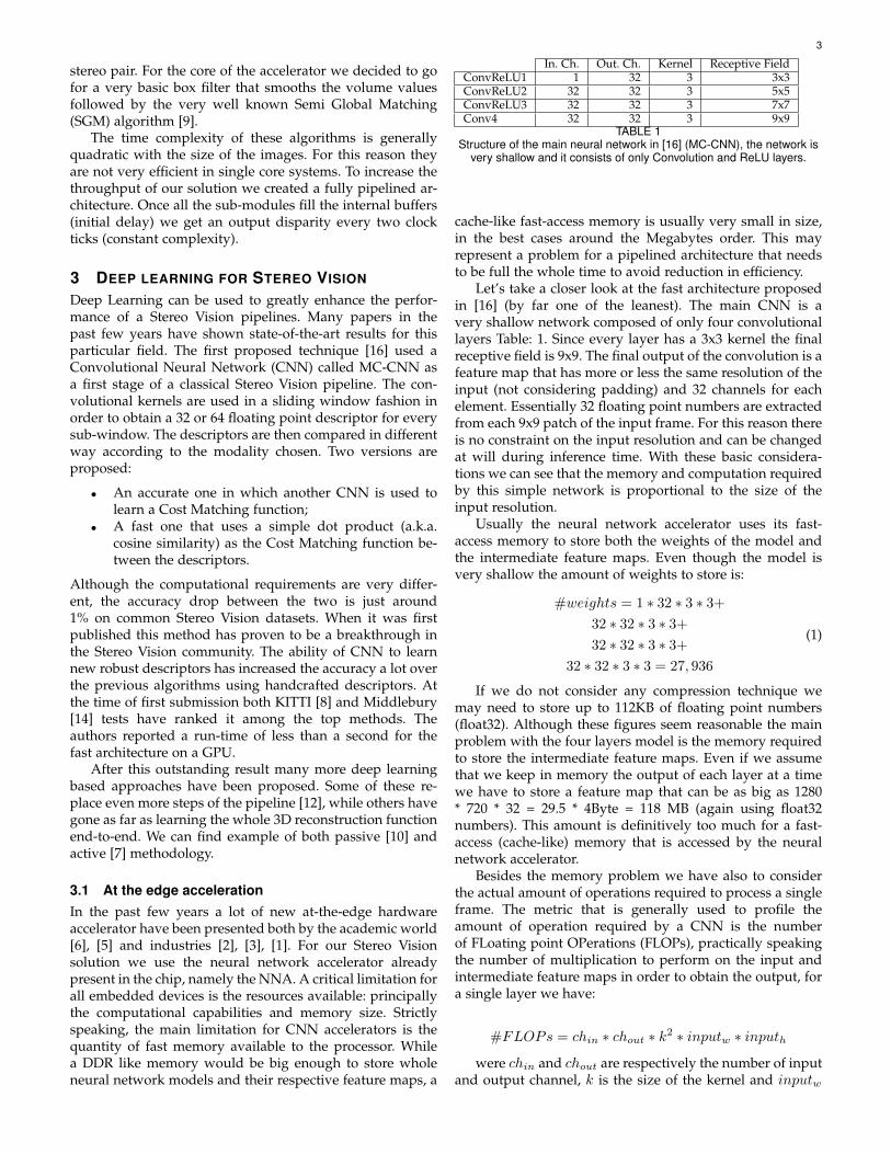
In. Ch. Out. Ch. Kernel Receptive FieldConvReLU1 1 32 3 3x3ConvReLU2 32 32 3 5x5ConvReLU3 32 32 3 7x7Conv4 32 32 3 9x9

TABLE 1Structure of the main neural network in [16] (MC-CNN), the network is

very shallow and it consists of only Convolution and ReLU layers.

cache-like fast-access memory is usually very small in size,in the best cases around the Megabytes order. This mayrepresent a problem for a pipelined architecture that needsto be full the whole time to avoid reduction in efficiency.

Let’s take a closer look at the fast architecture proposedin [16] (by far one of the leanest). The main CNN is avery shallow network composed of only four convolutionallayers Table: 1. Since every layer has a 3x3 kernel the finalreceptive field is 9x9. The final output of the convolution is afeature map that has more or less the same resolution of theinput (not considering padding) and 32 channels for eachelement. Essentially 32 floating point numbers are extractedfrom each 9x9 patch of the input frame. For this reason thereis no constraint on the input resolution and can be changedat will during inference time. With these basic considera-tions we can see that the memory and computation requiredby this simple network is proportional to the size of theinput resolution.

Usually the neural network accelerator uses its fast-access memory to store both the weights of the model andthe intermediate feature maps. Even though the model isvery shallow the amount of weights to store is:

#weights = 1 ∗ 32 ∗ 3 ∗ 3+

32 ∗ 32 ∗ 3 ∗ 3+

32 ∗ 32 ∗ 3 ∗ 3+

32 ∗ 32 ∗ 3 ∗ 3 = 27, 936

(1)

If we do not consider any compression technique wemay need to store up to 112KB of floating point numbers(float32). Although these figures seem reasonable the mainproblem with the four layers model is the memory requiredto store the intermediate feature maps. Even if we assumethat we keep in memory the output of each layer at a timewe have to store a feature map that can be as big as 1280* 720 * 32 = 29.5 * 4Byte = 118 MB (again using float32numbers). This amount is definitively too much for a fast-access (cache-like) memory that is accessed by the neuralnetwork accelerator.

Besides the memory problem we have also to considerthe actual amount of operations required to process a singleframe. The metric that is generally used to profile theamount of operation required by a CNN is the numberof FLoating point OPerations (FLOPs), practically speakingthe number of multiplication to perform on the input andintermediate feature maps in order to obtain the output, fora single layer we have:

#FLOPs = chin ∗ chout ∗ k2 ∗ inputw ∗ inputhwere chin and chout are respectively the number of input

and output channel, k is the size of the kernel and inputw

4

and inputh are the width and height of the input featuremap. Let’s consider the CNN used in [16] and a 720p HDinput frame (i.e. 1280×720): we have four layers with inputand output channels equals to 32 (except for the first inputchannel which is 1), all together:

#FLOPs = 1 ∗ 32 ∗ 9 ∗ 1280 ∗ 720+

32 ∗ 32 ∗ 9 ∗ 1280 ∗ 720+

32 ∗ 32 ∗ 9 ∗ 1280 ∗ 720+

32 ∗ 32 ∗ 9 ∗ 1280 ∗ 720 = 34× 109

(2)

This result has to be further multiplied by the numberof frames per second we want to obtain. No embeddedhardware accelerator in the market can reach this kindof performance. For this reason we searched for an evensmaller architecture.

The second problem to address is the complexity of thecomparison function used for the descriptor. In the originalfast architecture the cosine similarity is used. This functionis not really hardware friendly (a lot of multiplications anddivisions have to be performed). For this reason we decidedin favor of a binary descriptor. These kind of descriptor aremuch more compact and can be compared with a distancefunction as efficient as the hamming distance.

Finally the third problem to address is the computationaldemand of floating point multiplications. All the current at-the-edge hardware accelerators do not encourage the usageof floating point multiplication. In fact, it has been shownthat 8bit quantization can be used to fully replace fullprecision model with very low loss [4], [13]. This not onlydecreases the footprint of the model in the memory but italso allows the usage of smaller and much more efficient 8bit multiplier.

4 BINARY DESCRIPTORS

The first challenge we faced is the replacement of thefloating point descriptor with binary ones. For this reasonwe took [16] code-base and replaced the cosine similaritywith hamming distance. Since quantization loss is to beexpected we did different experiments to check how muchthe accuracy drops with a decreasing number of bits. Whatwe discovered is that even using a single bit for each floatnumber the accuracy of the output does not decrease toomuch.

The way we quantize a float number into a single bit isstraight forward, we simply threshold its value on zero, ifthe original number is bigger we set the bit to 1, 0 otherwise.We also tried to use the mean value for each output channelas a threshold but we found no improvement respect to asimple threshold on zero. Instead of 32 float feature vector(one for each output channel) we end up with an arrayof 32 bits. These are then compared in the Cost MatchingComputation using hamming distance. The accuracy dropwe got on KITTI dataset is very small, testing for KITTIerror metric T3 (all the pixel with a disparity value morewrong than 3 from the ground truth) the figures increasedfrom 4.875% to 4.887%. In this way the bandwidth betweenthe two modules decreases 118MB per frame to only 3.6MBper frame.

Fig. 2. Visual difference between cosine similarity (center) and hammingdistance (bottom) used for descriptor comparisons, the original front endfrom MC-CNN code base has been used. The two results are verysimilar, for this reason we dropped the less hardware friendly cosinesimilarity in favor of the more efficient hamming distance.

In Figure: 2 it is shown the actual difference betweenthe two results using different distance functions, the twofunctions give very similar results as long as the rest of thepipeline remains the same.

5 ABLATION STUDY

We explored different variations of the network in Table: 1.We first tried to decrease the number of input and outputchannels in different combinations of four and eight, withthe only exception for the last layer which still remains 32since we want a 32 bit descriptor. We choose four and eightmainly because the addressing and the scheduling for thesevalues its very hardware friendly. This reduces drasticallythe number of FLOPs required by the network. Unfortu-nately the main problem with a multilayer network is thenecessity to store the intermediate feature maps during thecomputation. Since in this use case the amount of memory isproportional to the resolution of the input image, it is verychallenging to find a solution for this particular problem.To satisfy the trade off between performance and accuracywe had to make big cut on the computational budget toallow a better data flow. We decided in favor a final modelwith a single layer network that has 32 kernel of 9x9 size,in this way the receptive field is kept constant respect tothe original model. Ablation studies were also performed in[16] in susbsection Hyperparameters, but it must be noticedthat a bigger kernel size has not been tested. The usage of asingle layer allows for on-the-fly computation: i.e. we don’thave to wait for the whole frame to be completely processed.Essentially we can start to send binary descriptors as soonas we process 9 lines of inputs. Our experiments haveshown little degradation in the final accuracy. In Figure: 3it is shown the difference between the original MC-CNNand the single layer one. The front end (cost computation,

5

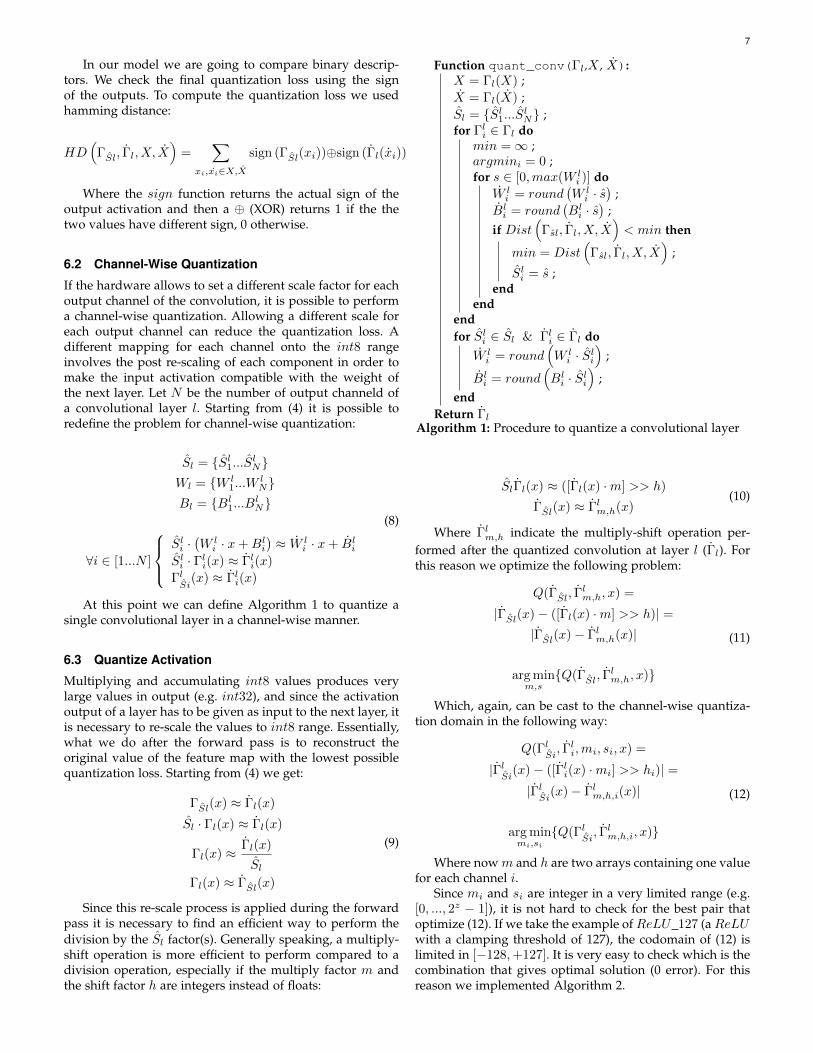
Fill Factor(%) T0.125(%) T0.25(%) T0.5(%) T0.75(%) T1(%) T2(%) T4(%) F0.5 F0.75 F1.0Kernel size: 3x3Ch.: 1,32,32,32,32 93.111 77.721 59.493 37.433 27.329 22.175 14.703 11.391 0.951 0.96 0.968

Kernel size: 3x3Ch: 1,4,4,8,32 92.124 78.169 60.56 38.925 29.169 24.224 16.67 13.113 0.942 0.953 0.963

Kernel size: 9x9Ch: 1,32 91.692 78.384 61.587 40.949 31.268 26.093 18.118 14.178 0.935 0.947 0.958

TABLE 2In the table are shown three different network topologies, the top row represent the original architecture from [16]: four layers with 32 channelseach. The middle row is the smallest four layers network we tried, the bottom row is the single layer network with the input of one channel and

output of 32. The dataset usd is MiddleburyV3 Quarter resolution. The metrics in the columns are respectively: the Fill Factor (which indicates theamount of non invalidated pixel), the TX metrics (which shows the percentage of disparities more wrong than X), the FX.X scores (which have the

classical definition).

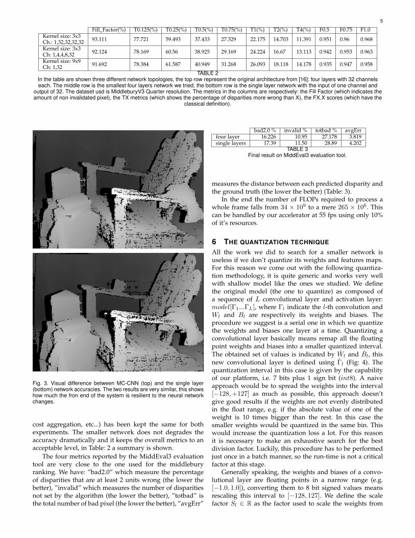
Fig. 3. Visual difference between MC-CNN (top) and the single layer(bottom) network accuracies. The two results are very similar, this showshow much the fron end of the system is resilient to the neural networkchanges.

cost aggregation, etc...) has been kept the same for bothexperiments. The smaller network does not degrades theaccuracy dramatically and it keeps the overall metrics to anacceptable level, in Table: 2 a summary is shown.

The four metrics reported by the MiddEval3 evaluationtool are very close to the one used for the middleburyranking. We have: ”bad2.0” which measure the percentageof disparities that are at least 2 units wrong (the lower thebetter), ”invalid” which measures the number of disparitiesnot set by the algorithm (the lower the better), ”totbad” isthe total number of bad pixel (the lower the better), ”avgErr”

bad2.0 % invalid % totbad % avgErrfour layer 16.226 10.95 27.178 3.819single layers 17.39 11.50 28.89 4.202

TABLE 3Final result on MiddEval3 evaluation tool.

measures the distance between each predicted disparity andthe ground truth (the lower the better) (Table: 3).

In the end the number of FLOPs required to process awhole frame falls from 34 × 109 to a mere 265 × 106. Thiscan be handled by our accelerator at 55 fps using only 10%of it’s resources.

6 THE QUANTIZATION TECHNIQUE

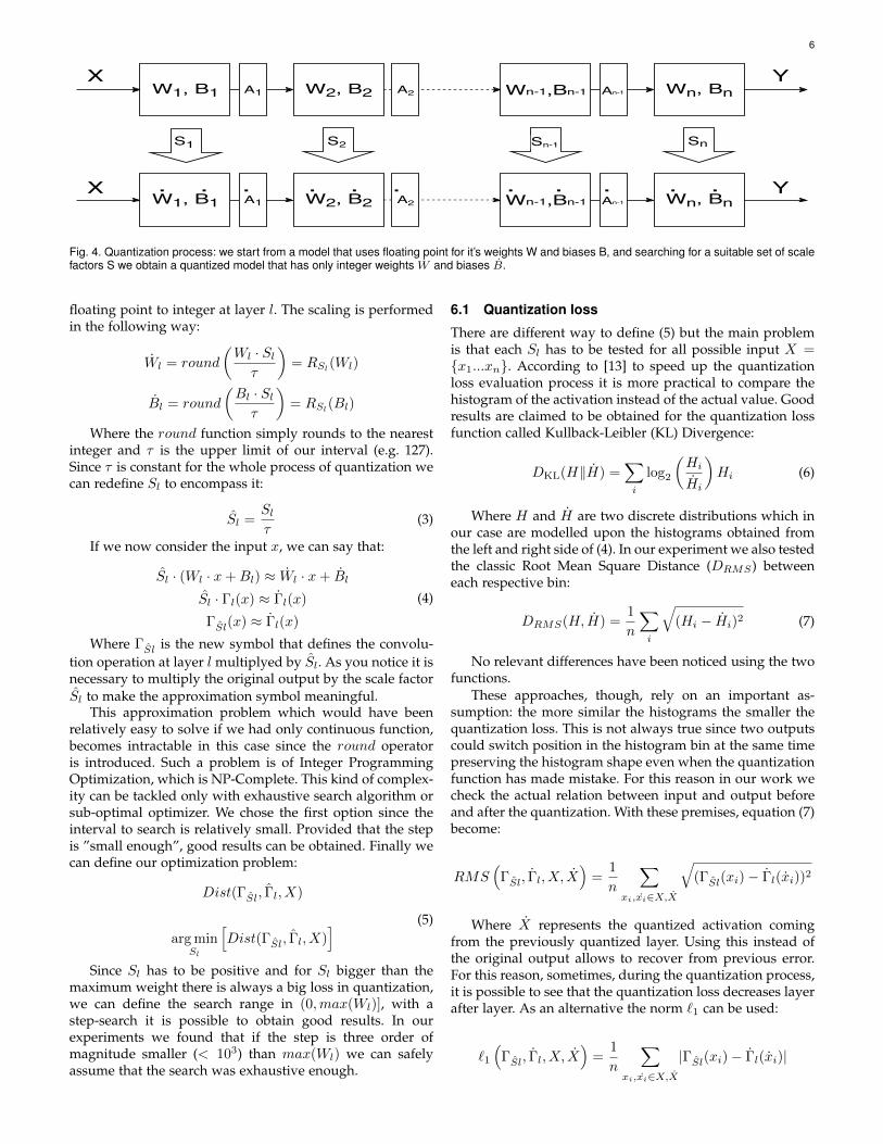
All the work we did to search for a smaller network isuseless if we don’t quantize its weights and features maps.For this reason we come out with the following quantiza-tion methodology, it is quite generic and works very wellwith shallow model like the ones we studied. We definethe original model (the one to quantize) as composed ofa sequence of L convolutional layer and activation layer:model[Γ1...ΓL], where Γl indicate the l-th convolution andWl and Bl are respectively its weights and biases. Theprocedure we suggest is a serial one in which we quantizethe weights and biases one layer at a time. Quantizing aconvolutional layer basically means remap all the floatingpoint weights and biases into a smaller quantized interval.The obtained set of values is indicated by Wl and Bl, thisnew convolutional layer is defined using Γl (Fig: 4). Thequantization interval in this case is given by the capabilityof our platform, i.e. 7 bits plus 1 sign bit (int8). A naiveapproach would be to spread the weights into the interval[−128,+127] as much as possible, this approach doesn’tgive good results if the weights are not evenly distributedin the float range, e.g. if the absolute value of one of theweight is 10 times bigger than the rest. In this case thesmaller weights would be quantized in the same bin. Thiswould increase the quantization loss a lot. For this reasonit is necessary to make an exhaustive search for the bestdivision factor. Luckily, this procedure has to be performedjust once in a batch manner, so the run-time is not a criticalfactor at this stage.

Generally speaking, the weights and biases of a convo-lutional layer are floating points in a narrow range (e.g.[−1.0, 1.0]), converting them to 8 bit signed values meansrescaling this interval to [−128, 127]. We define the scalefactor Sl ∈ R as the factor used to scale the weights from

6

W1, B1 W2, B2 Wn-1,Bn-1 Wn, BnA1 A2 An-1

W1, B1 W2, B2 Wn-1,Bn-1 Wn, BnA1 A2 An-1

 .      .      .          .      .      .                  .       .       .          .      .

S1 S2 Sn-1 Sn

X

X Y

Y

Fig. 4. Quantization process: we start from a model that uses floating point for it’s weights W and biases B, and searching for a suitable set of scalefactors S we obtain a quantized model that has only integer weights W and biases B.

floating point to integer at layer l. The scaling is performedin the following way:

Wl = round

(Wl · Sl

τ

)= RSl

(Wl)

Bl = round

(Bl · Sl

τ

)= RSl

(Bl)

Where the round function simply rounds to the nearestinteger and τ is the upper limit of our interval (e.g. 127).Since τ is constant for the whole process of quantization wecan redefine Sl to encompass it:

Sl =Sl

τ(3)

If we now consider the input x, we can say that:

Sl · (Wl · x+Bl) ≈ Wl · x+ Bl

Sl · Γl(x) ≈ Γl(x)

ΓSl(x) ≈ Γl(x)

(4)

Where ΓSl is the new symbol that defines the convolu-tion operation at layer l multiplyed by Sl. As you notice it isnecessary to multiply the original output by the scale factorSl to make the approximation symbol meaningful.

This approximation problem which would have beenrelatively easy to solve if we had only continuous function,becomes intractable in this case since the round operatoris introduced. Such a problem is of Integer ProgrammingOptimization, which is NP-Complete. This kind of complex-ity can be tackled only with exhaustive search algorithm orsub-optimal optimizer. We chose the first option since theinterval to search is relatively small. Provided that the stepis ”small enough”, good results can be obtained. Finally wecan define our optimization problem:

Dist(ΓSl, Γl, X)

arg minSl

[Dist(ΓSl, Γl, X)

] (5)

Since Sl has to be positive and for Sl bigger than themaximum weight there is always a big loss in quantization,we can define the search range in (0,max(Wl)], with astep-search it is possible to obtain good results. In ourexperiments we found that if the step is three order ofmagnitude smaller (< 103) than max(Wl) we can safelyassume that the search was exhaustive enough.

6.1 Quantization loss

There are different way to define (5) but the main problemis that each Sl has to be tested for all possible input X ={x1...xn}. According to [13] to speed up the quantizationloss evaluation process it is more practical to compare thehistogram of the activation instead of the actual value. Goodresults are claimed to be obtained for the quantization lossfunction called Kullback-Leibler (KL) Divergence:

DKL(H‖H) =∑i

log2

(Hi

Hi

)Hi (6)

Where H and H are two discrete distributions which inour case are modelled upon the histograms obtained fromthe left and right side of (4). In our experiment we also testedthe classic Root Mean Square Distance (DRMS) betweeneach respective bin:

DRMS(H, H) =1

n

∑i

√(Hi − Hi)2 (7)

No relevant differences have been noticed using the twofunctions.

These approaches, though, rely on an important as-sumption: the more similar the histograms the smaller thequantization loss. This is not always true since two outputscould switch position in the histogram bin at the same timepreserving the histogram shape even when the quantizationfunction has made mistake. For this reason in our work wecheck the actual relation between input and output beforeand after the quantization. With these premises, equation (7)become:

RMS(

ΓSl, Γl, X, X)

=1

n

∑xi,xi∈X,X

√(ΓSl(xi)− Γl(xi))2

Where X represents the quantized activation comingfrom the previously quantized layer. Using this instead ofthe original output allows to recover from previous error.For this reason, sometimes, during the quantization process,it is possible to see that the quantization loss decreases layerafter layer. As an alternative the norm `1 can be used:

`1(

ΓSl, Γl, X, X)

=1

n

∑xi,xi∈X,X

|ΓSl(xi)− Γl(xi)|

7

In our model we are going to compare binary descrip-tors. We check the final quantization loss using the signof the outputs. To compute the quantization loss we usedhamming distance:

HD(

ΓSl, Γl, X, X)

=∑

xi,xi∈X,X

sign (ΓSl(xi))⊕sign (Γl(xi))

Where the sign function returns the actual sign of theoutput activation and then a ⊕ (XOR) returns 1 if the thetwo values have different sign, 0 otherwise.

6.2 Channel-Wise Quantization

If the hardware allows to set a different scale factor for eachoutput channel of the convolution, it is possible to performa channel-wise quantization. Allowing a different scale foreach output channel can reduce the quantization loss. Adifferent mapping for each channel onto the int8 rangeinvolves the post re-scaling of each component in order tomake the input activation compatible with the weight ofthe next layer. Let N be the number of output channeld ofa convolutional layer l. Starting from (4) it is possible toredefine the problem for channel-wise quantization:

Sl = {Sl1...S

lN}

Wl = {W l1...W

lN}

Bl = {Bl1...B

lN}

∀i ∈ [1...N ]

Sli ·(W l

i · x+Bli

)≈ W l

i · x+ Bli

Sli · Γl

i(x) ≈ Γli(x)

ΓlSi

(x) ≈ Γli(x)

(8)

At this point we can define Algorithm 1 to quantize asingle convolutional layer in a channel-wise manner.

6.3 Quantize Activation

Multiplying and accumulating int8 values produces verylarge values in output (e.g. int32), and since the activationoutput of a layer has to be given as input to the next layer, itis necessary to re-scale the values to int8 range. Essentially,what we do after the forward pass is to reconstruct theoriginal value of the feature map with the lowest possiblequantization loss. Starting from (4) we get:

ΓSl(x) ≈ Γl(x)

Sl · Γl(x) ≈ Γl(x)

Γl(x) ≈ Γl(x)

Sl

Γl(x) ≈ ΓSl(x)

(9)

Since this re-scale process is applied during the forwardpass it is necessary to find an efficient way to perform thedivision by the Sl factor(s). Generally speaking, a multiply-shift operation is more efficient to perform compared to adivision operation, especially if the multiply factor m andthe shift factor h are integers instead of floats:

Function quant_conv(Γl,X , X):X = Γl(X) ;X = Γl(X) ;Sl = {Sl

1...SlN} ;

for Γli ∈ Γl do

min =∞ ;argmini = 0 ;for s ∈ [0,max(W l

i )] doW l

i = round(W l

i · s)

;Bl

i = round(Bl

i · s)

;if Dist

(Γsl, Γl, X, X

)< min then

min = Dist(

Γsl, Γl, X, X)

;

Sli = s ;

endend

endfor Sl

i ∈ Sl & Γli ∈ Γl do

W li = round

(W l

i · Sli

);

Bli = round

(Bl

i · Sli

);

endReturn Γl

Algorithm 1: Procedure to quantize a convolutional layer

SlΓl(x) ≈ ([Γl(x) ·m] >> h)

ΓSl(x) ≈ Γlm,h(x)

(10)

Where Γlm,h indicate the multiply-shift operation per-

formed after the quantized convolution at layer l (Γl). Forthis reason we optimize the following problem:

Q(ΓSl, Γlm,h, x) =

|ΓSl(x)− ([Γl(x) ·m] >> h)| =|ΓSl(x)− Γl

m,h(x)|

arg minm,s

{Q(ΓSl, Γlm,h, x)}

(11)

Which, again, can be cast to the channel-wise quantiza-tion domain in the following way:

Q(ΓlSi, Γl

i,mi, si, x) =

|ΓlSi

(x)− ([Γli(x) ·mi] >> hi)| =

|ΓlSi

(x)− Γlm,h,i(x)|

arg minmi,si

{Q(ΓlSi, Γl

m,h,i, x)}

(12)

Where now m and h are two arrays containing one valuefor each channel i.

Since mi and si are integer in a very limited range (e.g.[0, ..., 2z − 1]), it is not hard to check for the best pair thatoptimize (12). If we take the example ofReLU 127 (aReLUwith a clamping threshold of 127), the codomain of (12) islimited in [−128,+127]. It is very easy to check which is thecombination that gives optimal solution (0 error). For thisreason we implemented Algorithm 2.

8

Fill Factor(%) T0.125(%) T0.25(%) T0.5(%) T0.75(%) T1(%) T2(%) T4(%) F0.5 F0.75 F1.0Kernel size: 9x9Ch: 1,32 91.692 78.384 61.587 40.949 31.268 26.093 18.118 14.178 0.935 0.947 0.958

Kernel size: 9x9Ch: 1,32Quantized

91.746 78.387 61.615 40.993 31.35 26.158 18.155 14.21 0.934 0.947 0.958

TABLE 4Accuracy drop due to the quantization loss in the single layer network. The dataset used is MiddleburyV3 Quarter resolution

Function quant_act(ΓSl, Γl, X):m = {m1, ...,mN} ;h = {h1, ..., hN} ;for Sl

i ∈ Sl dofor M = [0, ..., 2z − 1] do

for H = [0, ..., 2z − 1] doif Q(Γl

Si, Γl

M,H,i, X) < min thenmin = Q(Γl

Si, Γl

M,H,i, X) ;mi = M ;hi = H ;

endend

endend

Return m,hAlgorithm 2: Procedure to quantize the activation

Depending on the activation function (ReLU, Sigmoid,Tanh, ...) different scaling can be applied. With ReLU thereare not many problems since we minimize the differencebetween non-quantized and quantized output, this meansthat positive values will stay positive and vice-versa, if thevalue is close to 0 the activation will be not dramaticallychanged. A different challenge is for Sigmoid and Tanhwhich have a narrow non-saturation interval, scaling thisinterval proportionally to S solves the problem. After thatthe activation and scaling is applied, the big values are againin int8 format.

6.4 The algorithm

At this point we can put all together, quantizing one layer ata time, the convolution and then the activation, it is possibleto obtain very close result even if we scaled from float toint8.

Function Quantization(model[Γ1, ...,ΓL], X):model[Γ1, ..., ΓL] ;X = X ;for Γl ∈ model[Γ1, ...,ΓL] do

Γl = quant conv(Γl, X, X) ;Γlm,h = quant act(ΓSl, Γl, X) ;X = Γl(X) ;X = Γl

m,h(X) ;end

Return model[Γ1m,h, ..., Γ

Lm,h]

Algorithm 3: Procedure to quantize the activation

As you can see in Algorithm 3, the input is forwardedthrough the original network as a reference. The final met-

bad0.5 bad2.0 rms avgerrnonocc dense 60.2 22.8 19.7 6.34nonocc sparse 51.1 15.5 14 3.86all dense 64.4 29.6 29.7 11.2all sparse 48.6 17 20 6.29

TABLE 5Results reported by the Middlebury page rank.

rics reported for the choosen quantized network are shonwin Table: 4

7 RESULTS

We finally compare our solution with the state-of-the-artapproaches, for this reason we submitted our disparitymaps to the Middlebury ranking. Currently our methodranks half way of the ranking and it is the first among allthe ASICs. In Table: 5 are shown the metrics we obtained:

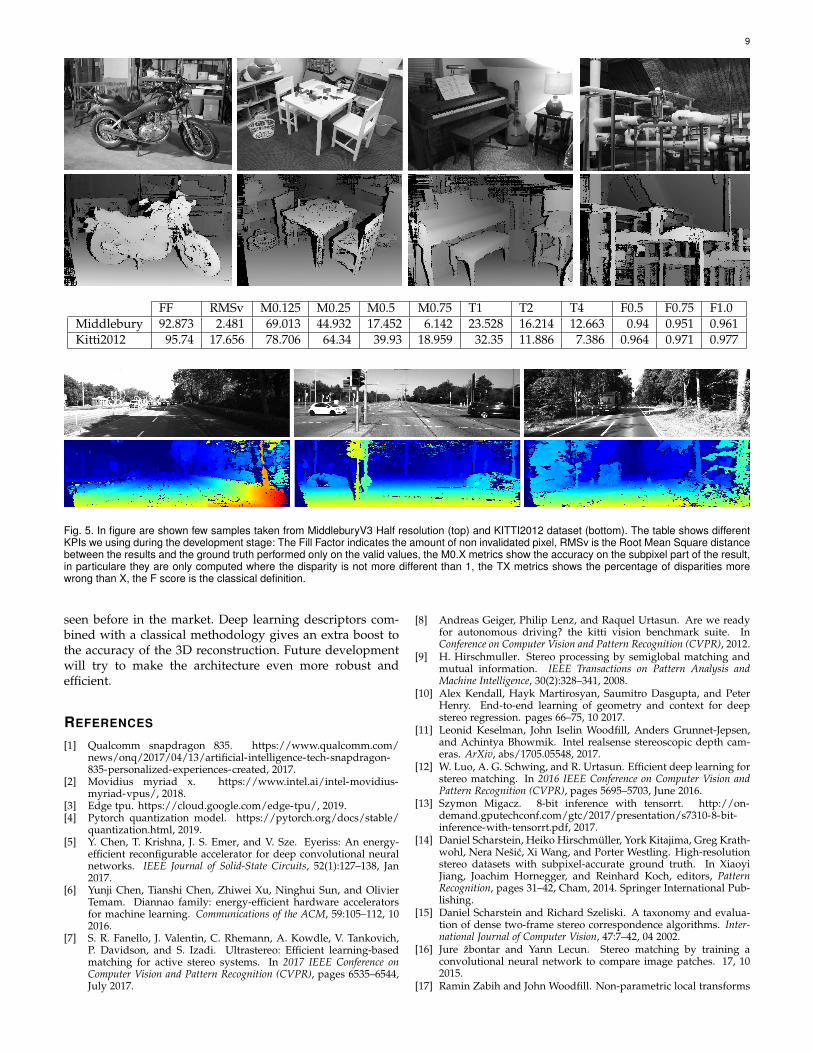
The ranking measures a lot of metrics for differentsetup, the main difference between the setups is what it isconsidered for evaluation: we have a setup that considersonly the non occluded pixel in the ground truth (nonocc)and one that considers all pixels. Furthermore the testingtools try to evaluate the metrics with the original results(sparse) and with a cleverly filled version (dense). Since thealgorithm is capable of subpixel resolution also bad0.5 isshown. This one counts the percentage of disparities thatare more wrong than 0.5 units of disparity. For a morecomprehensive summary refer to Figure: 5.

7.1 PerformanceSince the architecture is divided in two main modules wemust distinguish between the performance of the NNA andthe SVA. The NNA will only run the trained CNN, thismodule has to process the two frames coming from thecameras. For parallelism reasons the NNA is composed of10 submodules, using one of this submodule it is possible toprocess 55 frames with 720p resolution (1280 × 720). Usingonly two submodules it is possible to reach more than realtime performance. The SVA instead is far more efficient. Itcan process up to 250fps in left-right check mode. Practicallyspeaking the module can be used for multiple camera pairsat the same time. This differentiation makes different usecases possible. While it is true that we might have the wholeNNA and SVA processing stereo pairs of frame, we can alsouse a parte of the NNA to process a single disparity mapand use the rest of the NNA to accelerate a deep learningbased recognition algorithm.

8 CONCLUSION

The accuracy and performance given by our new architec-ture of passive Stereo Vision system is increased as never

9

FF RMSv M0.125 M0.25 M0.5 M0.75 T1 T2 T4 F0.5 F0.75 F1.0Middlebury 92.873 2.481 69.013 44.932 17.452 6.142 23.528 16.214 12.663 0.94 0.951 0.961Kitti2012 95.74 17.656 78.706 64.34 39.93 18.959 32.35 11.886 7.386 0.964 0.971 0.977

Fig. 5. In figure are shown few samples taken from MiddleburyV3 Half resolution (top) and KITTI2012 dataset (bottom). The table shows differentKPIs we using during the development stage: The Fill Factor indicates the amount of non invalidated pixel, RMSv is the Root Mean Square distancebetween the results and the ground truth performed only on the valid values, the M0.X metrics show the accuracy on the subpixel part of the result,in particulare they are only computed where the disparity is not more different than 1, the TX metrics shows the percentage of disparities morewrong than X, the F score is the classical definition.

seen before in the market. Deep learning descriptors com-bined with a classical methodology gives an extra boost tothe accuracy of the 3D reconstruction. Future developmentwill try to make the architecture even more robust andefficient.

REFERENCES

[1] Qualcomm snapdragon 835. https://www.qualcomm.com/news/onq/2017/04/13/artificial-intelligence-tech-snapdragon-835-personalized-experiences-created, 2017.

[2] Movidius myriad x. https://www.intel.ai/intel-movidius-myriad-vpus/, 2018.

[3] Edge tpu. https://cloud.google.com/edge-tpu/, 2019.[4] Pytorch quantization model. https://pytorch.org/docs/stable/

quantization.html, 2019.[5] Y. Chen, T. Krishna, J. S. Emer, and V. Sze. Eyeriss: An energy-

efficient reconfigurable accelerator for deep convolutional neuralnetworks. IEEE Journal of Solid-State Circuits, 52(1):127–138, Jan2017.

[6] Yunji Chen, Tianshi Chen, Zhiwei Xu, Ninghui Sun, and OlivierTemam. Diannao family: energy-efficient hardware acceleratorsfor machine learning. Communications of the ACM, 59:105–112, 102016.

[7] S. R. Fanello, J. Valentin, C. Rhemann, A. Kowdle, V. Tankovich,P. Davidson, and S. Izadi. Ultrastereo: Efficient learning-basedmatching for active stereo systems. In 2017 IEEE Conference onComputer Vision and Pattern Recognition (CVPR), pages 6535–6544,July 2017.

[8] Andreas Geiger, Philip Lenz, and Raquel Urtasun. Are we readyfor autonomous driving? the kitti vision benchmark suite. InConference on Computer Vision and Pattern Recognition (CVPR), 2012.

[9] H. Hirschmuller. Stereo processing by semiglobal matching andmutual information. IEEE Transactions on Pattern Analysis andMachine Intelligence, 30(2):328–341, 2008.

[10] Alex Kendall, Hayk Martirosyan, Saumitro Dasgupta, and PeterHenry. End-to-end learning of geometry and context for deepstereo regression. pages 66–75, 10 2017.

[11] Leonid Keselman, John Iselin Woodfill, Anders Grunnet-Jepsen,and Achintya Bhowmik. Intel realsense stereoscopic depth cam-eras. ArXiv, abs/1705.05548, 2017.

[12] W. Luo, A. G. Schwing, and R. Urtasun. Efficient deep learning forstereo matching. In 2016 IEEE Conference on Computer Vision andPattern Recognition (CVPR), pages 5695–5703, June 2016.

[13] Szymon Migacz. 8-bit inference with tensorrt. http://on-demand.gputechconf.com/gtc/2017/presentation/s7310-8-bit-inference-with-tensorrt.pdf, 2017.

[14] Daniel Scharstein, Heiko Hirschmuller, York Kitajima, Greg Krath-wohl, Nera Nesic, Xi Wang, and Porter Westling. High-resolutionstereo datasets with subpixel-accurate ground truth. In XiaoyiJiang, Joachim Hornegger, and Reinhard Koch, editors, PatternRecognition, pages 31–42, Cham, 2014. Springer International Pub-lishing.

[15] Daniel Scharstein and Richard Szeliski. A taxonomy and evalua-tion of dense two-frame stereo correspondence algorithms. Inter-national Journal of Computer Vision, 47:7–42, 04 2002.

[16] Jure zbontar and Yann Lecun. Stereo matching by training aconvolutional neural network to compare image patches. 17, 102015.

[17] Ramin Zabih and John Woodfill. Non-parametric local transforms

10

for computing visual correspondence. In Jan-Olof Eklundh, editor,Computer Vision — ECCV ’94, pages 151–158, Berlin, Heidelberg,1994. Springer Berlin Heidelberg.

[18] Zhengyou Zhang. Microsoft kinect sensor and its effect. IEEEMultiMedia, 19:4–12, April 2012.