18

The Theory of Edge Detection and Low-level Vision in Retrospect

Kuntal Ghosh 1 , Sandip Sarkar 2 and Kamales Bhaumik 3

1Indian Statistical Institute, 2Saha Institute of Nuclear Physics,

3West Bengal University of Technology India.

1. Introduction

Talking about human eye and how its astounding complexity seemingly challenged the very laws of evolution, Charles Darwin observed the following while discussing about “organs of extreme perfection and complication”, in the Chapter VI titled Difficulties of the Theory of his revolutionary work, The Origin of Species:“To suppose that the eye with all its inimitable contrivances for adjusting the focus to different distances, for admitting different amounts of light, and for the correction of spherical and chromatic aberration, could have been formed by natural selection, seems, I freely confess, absurd in the highest degree. When it was first said that the sun stood still and the world turned round, the common sense of mankind declared the doctrine false; but the old saying of Vox populi, vox Dei, as every philosopher knows, cannot be trusted in science. Reason tells me, that if numerous gradations from a simple and imperfect eye to one complex and perfect can be shown to exist, each grade being useful to its possessor, as is certainly the case; if further, the eye ever varies and the variations be inherited, as is likewise certainly the case and if such variations should be useful to any animal under changing conditions of life, then the difficulty of believing that a perfect and complex eye could be formed by natural selection, though insuperable by our imagination, should not be considered as subversive of the theory. ” The purpose of the present chapter would be to understand and explain some of the aspects of this highly complicated organ and how it is likely to coordinate with the brain at the stage of early vision. Pioneering contributions in this domain came from renowned philosophers and vision scientists like Wilhelm Wundt, Hermann von Helmholtz (Helmholtz, 1867) and Ernst Mach (Mach, 1865). The British empiricist school of Locke, Hume and Berkeley led to the structuralist viewpoint of Wundt and the empirio-critical view of Mach, that defined visual perception as a process arising out of certain basic sensory atoms which act as primitive, indivisible elements of visual experience spanning each tiny localized region of the visual field, presumably resulting from the activity of the individual rods and cones in the retina. Analogous to the structural relation between primitive atoms and the more complex molecules, this structuralist theory relied upon the concept of gluing together of

Source: Vision Systems: Segmentation and Pattern Recognition, ISBN 987-3-902613-05-9,Edited by: Goro Obinata and Ashish Dutta, pp.546, I-Tech, Vienna, Austria, June 2007

Vision Systems - Segmentation and Pattern Recognition 354

many simple sensations (like colour) into more complex perceptions of a whole entity.As a reaction to such mechanical materialist viewpoint arose the Gestalt movement that was led by Max Wertheimer who in the guise of rejecting the structuralist viewpoint, actually attacked the very base of scientific materialist viewpoint by claiming that perceptions can only have their own intrinsic whole structures that cannot, by any means, be reduced to parts or even to piecewise relations among the parts. As evidence of holism, Gestaltists pointed to those examples in which configurations have emergent properties, not shared by any of their local parts. Thus, while the structuralist viewpoint represented an inconsistent materialistic approach where “part” assumes the role of almighty and the “whole” is merely its follower, the Gestalt school on the other resorted to idealism where “part” is devoid of any identity with respect to “whole”. The dialectical relation between part and whole that is the science of transformation of quantity to quality, which is responsible for any emergent behaviour was temporarily dissolved in the fog of subjectivism, until the time was ripe for the advancement of science and philosophy to free the domain of vision science from such cloaks of mysticism. Emerged a new school of vision scientists to whom vision is first and foremost, an information-processing task whose study should invariably include not just how to extract from images the various aspects of the world that are useful to us, but also an enquiry into the nature of internal representations by which we capture this information and make it available for processing as a basis for decisions about our thoughts and actions. The use of computer simulations to model the cognitive processes, the application of information processing approach to psychology and the rapid advancement in neurophysiological techniques that led to the emergence of the idea that the eye-brain system is a biological processor of information, changed the way in which scientists understood vision. The remarkable works of Golgi, Cajal, Adrian, Granit, Hartline and other physiologists along with the advent of the modern computer age led by Alan Turing and John von Neumann served to establish the fact that starting from the two dimensional intensity array formation on the retina to the three dimensional object reconstruction and recognition in higher regions of the brain, the entire process is controlled and executed by networks of neurons of different types and that there is no “soul” sitting anywhere and interpreting things from the neuronal outputs. Rather visual perception is a collective, step-by-step synchronization of the outputs at various stages in the eye and the brain, no matter how complex that process is. It was this approach that led to the notion of a cell’s “receptive field” that becomes evident so clearly from the study by H. B. Barlow of the ganglion cells of the frog retina where he said (Barlow, 1953): “If one explores the responsiveness of single ganglion cells in the frog’s retina using handheld targets, one finds that one particular type of ganglion cell is most effectively driven by something like a black disc subtending a degree or so moved rapidly to and fro within the unit’s receptive field. ” The corresponding mathematical approach of creating computer programs to extract useful information about the environment from optical images was articulated most effectively by David Marr and his colleagues (Marr, 1982). It dealt in details with how the luminance structure in two-dimensional images may provide information about the structure of surfaces and objects in three-dimensional space, though the pioneering mathematical analysis in this field was contributed by the Dutch physicists Jan Koenderink and Andrea van Doorn who dealt with sophisticated mathematical techniques from differential

The Theory of Edge Detection and Low-level Vision in Retrospect 355

geometry to the three dimensional orientation of surfaces from shading information. But in this chapter we shall restrict ourselves only to the receptive field structure relevant to the Theory of edge detection (Marr & Hildreth, 1980) that, according to its authors, is responsible for a “raw primal sketch” of the world around us. For this, we first elucidate a few basic things associated with the processing of the digital images by computers, which would be extensively used in the present chapter.

2. Preliminary Concepts in Computer Vision

An image is a two-dimensional representation of a three dimensional object or scenario. A monochrome image is characterised by a continuous intensity function ),( yxI at every point

),( yx in the image plane. The final goal of image processing is to extract information from ),( yxI to reconstruct the 3-D view of the original object or scenario. In a digital image the

abstract concept of points is replaced by a realistic concept of infinitesimal identical areas (such as pixels in a computer screen). These infinitesimal areas span the entire image plane and are numbered in an ordered fashion both horizontally and vertically. Moreover, the continuous intensity function is replaced by values from a discrete gray scale. As a result the continuous intensity function ),( yxI is replaced by a discrete function ),( ii yxI , in which ),( ii yx denotes the pixel position and ),( ii yxI denotes the average discrete gray scale value of that pixel. Let us now discuss the salient points about the concept of an edge. Location of an edge is the most crucial information that is to be extracted during the primary processing of any image. Any sharp change of intensity qualifies for an edge (Fig. 1a). Accurate detection of these transitions along with their correct locations is the purpose of edge detection algorithms. In a digital image an edge occurs at the boundary between two pixels provided the gray values of the pixels differ considerably from one another. From the vagueness of the word “considerably” it is obvious that identification of an edge is a subjective procedure. In one extreme any difference of intensity may be assumed to be an edge, so that the processed image would become a messy assemblage of edges leaving no scope for feature extraction. In its other extreme, the important edges may get lost thereby forsaking valuable information. Sudden transition of a continuous function is best identified by differentiating it, which gives a large value at the point of transition and zero value at the points of no transition. For a discrete function, the differentiation operation is replaced by difference operation. One can use either first order directional derivatives, like x∂∂ or y∂∂ in which case one would have to search for their crests and troughs at each orientation (Fig. 1b) when applied to a 2-D image, or one can also use second order directional derivatives, like

22 x∂∂ or 22 y∂∂ in which case the directional intensity change would correspond to their zero-crossings (Fig. 1c). Using finite difference approximation, the corresponding spatial organizations for some these operators or “receptive fields” as they are neurophysiologically termed, are displayed below:

≡∂∂ x -1 +1 ≡∂∂ 22 x -1 +2 -1

Vision Systems - Segmentation and Pattern Recognition 356

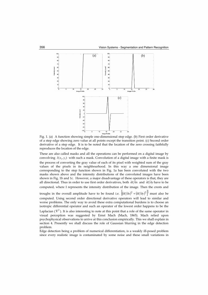
Fig. 1. (a) A function showing simple one-dimensional step edge. (b) First order derivative of a step edge showing zero value at all points except the transition point. (c) Second order derivative of a step edge. It is to be noted that the location of the zero crossing faithfully reproduces the location of the edge.

These are also called masks and all the operations can be performed on a digital image by convolving ),( ii yxI with such a mask. Convolution of a digital image with a finite mask is the process of converting the gray value of each of its pixel with weighted sum of the gray values of the pixels in its neighbourhood. In this way a one dimensional image corresponding to the step function shown in Fig. 1a has been convoluted with the two masks shown above and the intensity distributions of the convoluted images have been shown in Fig. 1b and 1c. However, a major disadvantage of these operators is that, they are all directional. Thus in order to use first order derivatives, both xI ∂∂ and yI ∂∂ have to be computed, where I represents the intensity distribution of the image. Then the crests and

troughs in the overall amplitude have to be found i.e. ( ) ( )[ ]2122 yIxI ∂∂+∂∂ must also be computed. Using second order directional derivative operators will lead to similar and worse problems. The only way to avoid these extra computational burdens is to choose an isotropic differential operator and such an operator of the lowest order happens to be the Laplacian ( 2∇ ). It is also interesting to note at this point that a role of the same operator in visual perception was suggested by Ernst Mach (Mach, 1865). Mach relied upon psychophysical observations to arrive at this conclusion empirically. This we shall explain in section 4. Presently we shall discuss the role of Gaussian blurring in the edge detection problem.Edge detection being a problem of numerical differentiation, is a weakly ill-posed problem since every realistic image is contaminated by some noise and these small variations in

(a) (b)

(c)

The Theory of Edge Detection and Low-level Vision in Retrospect 357

input lead to large changes in output. Since a noise point has a likelihood of having an intensity difference with its neighbours, in edge analysis this may create spurious edge points. It is, therefore, desirable that before processing the image, the intensity of a noise point should be brought closer to the intensity of its neighbourhood. Any filter operated over the image to achieve such a smoothing should make the spatial variation of intensity as small as possible or in other words the spatial variance xΔ of the filter should be small. On the other hand, the filter’s spectrum should be band-limited in the frequency domain. Consequently its variance ωΔ should also be small. There is a conflict between these two

localisations through an uncertainty principle:4

πω ≥ΔΔx . The only function that optimises

this relation is the Gaussian function. This is the reason why the images are generally smoothened by convolving with a Gaussian function prior to the differentiation operation. A one-dimensional Gaussian function is defined as:

2

2

21

2

1),( σ

σπσ

x

exG−

= ,

so that =1),( dxxG σ

(1)

Here σ is the standard deviation (or scale parameter) of the Gaussian function. Convolution of an image with the Gaussian function effectively wipes out all structures at scales smaller than the space constant σ of the Gaussian function. It may easily be verified that the Fourier transform of a Gaussian function is also a Gaussian. In 2-D, the Gaussian is defined as:

2

2

222

1),( σ

πσσ

r

erG−

= , with 222 yxr +=

(2)

For an image, the Gaussian filtering has the added advantages. Since a 2-D Gaussian function is rotationally symmetric, it preserves the neighbourhood characteristics both in the spatial and frequency domain. It is also computationally handy because it can be decomposed into two 1-D Gaussians i.e. )()(),( yGxGyxG = . In fact Gaussian is the only rotationally symmetric function that is separable. The two types of filters, discussed above viz. the derivative operator and the smoothing operator, are both used extensively in digital image processing. In effect, initially the unwanted noises are to be removed (smoothened) from the image by convoluting it with a Gaussian function. Then a derivative filter is operated to detect the edge points. From the discussion presented above, it is becoming increasingly clear why in their classical theory of edge detection (Marr & Hildreth, 1980), the authors argued in favour of the Laplacian of Gaussian ( G2∇ ) based structure of receptive field. But before we deal with this operator in more detail, it is first important to look into the mechanism of image processing in mammalian eye and what the receptive field is.

3. A Brief Overview of Mammalian Retina

It is known from neurophysiological experiments on cat and monkey that a good deal of processing of images falling on the eye occurs in the retina and primary visual cortex itself. This is known as primary or low-level visual processing. We shall now give a brief overview of the physiology related to primary visual processing and its role in edge detection.

Vision Systems - Segmentation and Pattern Recognition 358

Fig. 2 A schematic drawing showing the retinal network. Rods and cones, known as photoreceptors, receive the light, get excited, send information to the bipolar cells, either directly or through the network of horizontal cells. The bipolar cells, in their turn, send information to ganglion cells, again either directly or through the network of amacrine cells. From ganglion cells the information travels to the primary visual cortex through optic nerves.

In the mammalian retina, the primary photoreceptors are the rods and cones (Fig. 2), which are spread over a surface. For simplicity if we neglect the aspect of colour, the retinal images can be approximated by ),( ii yxI as argued in the previous section. Classical investigations by neurophysiologists have shown that information about the input image is extracted in the successive layers of the retina (Fig. 3a). For example, a bipolar cell receives information from a large number of photoreceptors distributed over a circular zone, mainly through a network of horizontal cells and the ganglion cell receives information from the bipolar cells through another network of amacrine cells. It is easy to understand that any particular bipolar or ganglion cell cannot receive information from all the photoreceptors (rods and cones) of the entire retina. Only a small area of the retina would be responsible for eliciting response in that cell. That area (assumed to be circular or elliptical in shape) is called the receptive field of that bipolar or ganglion cell. A schematic diagram is shown in Fig. 3b. Physiologists further observed that while the receptors in the central region of this zone send information to a bipolar cell in a positive fashion, the information from the peripheral cells arrives with a reversal of signature (Fig. 4). As a result a central bright spot with dark background is the best stimulus for exciting the bipolar cell. (These bipolar cells are known as on-centre cells. There are also off-centre bipolar cells for which a dark spot with bright background is the most appropriate stimulus.) Information of such an antagonistic effect from a large number of bipolar cells is collected and transmitted by the ganglion cells. For simplicity in understanding the organization of a receptive field structure, let us consider a one-dimensional retina in which the photoreceptors are spread over a line. Strength of the output from a photoreceptor to the ganglion cell should be maximum when the two cells are in closest proximity. It is also natural to assume that the contributions

The Theory of Edge Detection and Low-level Vision in Retrospect 359

Fig. 3 (a) Information processing occurs in the retina through successive layers. (b) Receptive field of a bipolar or ganglion cell is a circular or elliptical area on the photoreceptor layer that elicit response in that cell

Fig. 4 The classical excitatory-inhibitory centre-surround receptive field structure of retinal bipolar and ganglion cells.

Rods and Cones

Bipolarcells

Ganglioncells

(a)

ReceptiveField

(b)

+ve -ve-ve

Vision Systems - Segmentation and Pattern Recognition 360

Fig. 5. The centre and surround responses of a ganglion cell has been fitted with two Gaussian curves in opposite phase. The surround is represented by a broader Gaussian compared to the central one

received by a ganglion cell from other receptors will smoothly fall off with the distance. Such a distribution can be safely assumed to be a Gaussian. This would be true for both positive (centre) and negative (surround) inputs (Fig. 5). Consequently the net input to a ganglion cell is obtained from a difference of two Gaussian inputs, the central one (positive) having a smaller variance than the surround (negative). This prompted the physiologists to develop a model of Difference of Gaussian or DOG for the receptive field of retinal ganglion cells. A DOG function in one dimension, will be:

+ve contribution-ve -ve

Distance

Intensity of signal

-2 -1 0 1 2

+ve contribution-ve -ve

The Theory of Edge Detection and Low-level Vision in Retrospect 361

22

2

21

2

2

2

2

1

212

1

2

1),(

σσ

σπσπσσ

xx

eeDOG−−

−= (3)

This model can be easily extended for two-dimensional images by using 2-D Gaussians. The DOG model is very effective in explaining a large number of experimental findings in retinal responses as we shall see in sections 4 and 5.3. Essentially DOG is the classical model for the centre-surround antagonistic effects observed at the retinal ganglion cell.

4. The Classical Receptive Field and Theory of Edge Detection

As discussed previously, from the computational point of view the most natural filter for edge detection should have a combination of derivative and smoothening filter. As established before, a Laplacian of Gaussian (LOG) filter is the best alternative for combining the smoothening and derivative operation for the image. Laplacian operated on a 2-D Gaussian will give:

2

2

22

2

2

2

21

1),( σ

σπσσ

r

errG−

−−=∇ (4)

Marr and Hildreth (Marr & Hildreth, 1980) further argued that for a certain ratio of the scale parameters in DOG (i.e. for a certain value of 21 :σσ ), LOG can be considered to be a good approximation to DOG. We have already said that even without any knowledge of the DOG based classical receptive field structure from physiologists, since those experiments were actually performed almost a century after he carried out his psychophysical experiments, Ernst Mach, could still visualize empirically the centre-surround structure in retina and predict the Laplacian operation in early vision as well. This is what Mach said (Mach, 1865): “The illumination of a retinal point will, in proportion to the difference between this illumination and the average of the illumination on neighboring points, appear brighter or darker, respectively depending on whether the illumination of it is above or below the average. The weight of the retinal points in this average is to be thought of as rapidly decreasing with distance from the particular point considered.” Furthermore, he went on to state: “Let us call the intensity of illumination ),( yxfu = . The brightness sensation v of the corresponding retinal point is given by

)( 2222 dyuddxudmuv +−= (5)

where m is a constant. If the expression in parentheses is positive, then the sensation of brightness is reduced; in the opposite case, it is increased. Thus, v is not only influenced by u , but also its second differential coefficients.” Let us now see, what led Mach to arrive at such revolutionary conclusions on visual perception. Mach was experimenting with rotating white discs with black sectors of varying size, when he came across the phenomenon that is now commonly referred to as Mach band illusion. The most commonly used image for understanding the Mach band illusion is shown in Fig. 6a. By scanning this image in a direction in which the luminance increases or

Vision Systems - Segmentation and Pattern Recognition 362

decreases our visual system perceives an actually non-existent darker bar at the location where the figure just starts getting lighter. Similarly, a brighter bar is perceived at the point where brightness just stops increasing. However, a horizontal line scan of this image (Fig. 6b) clearly establishes that what we see is a mere illusion and the image represents a simple staircase function only devoid of any special border effect. It was the observation of this illusory phenomenon that prompted Mach to arrive at his inferences quoted above. In order

Fig. 6 (a) The Mach band illusion of dark and bright borders around bright and dark regions respectively (b) A horizontal profile of this image is obviously a simple staircase function that bears no signature of the illusory perception.

to conceive Mach’s arguments let us resort to the receptive field mode of spatial organizations of the Laplacian operator as has been initiated for derivative operators in section 2. We have stated there that a finite difference approximation of the horizontal directional second order partial derivative, 22 x∂∂ may be written as:

Consequently, the vertical directional operator 22 y∂∂ may be represented by the transpose of the above vector. When these two are combined together, we obtain the kernel for the isotropic 2∇ (i.e. 2222 yx ∂∂+∂∂ ) operator:

Using the property of isotropicity of the Laplacian opeartor, the diagonal directions are now incorporated by taking the co-ordinates along these directions applying a 045 rotation so that we arrive at a new kernel:

≡∂∂ 22 x -1 +2 -1

0 -1 0

-1 4 -1

0 -1 0

(a)

(b)

The Theory of Edge Detection and Low-level Vision in Retrospect 363

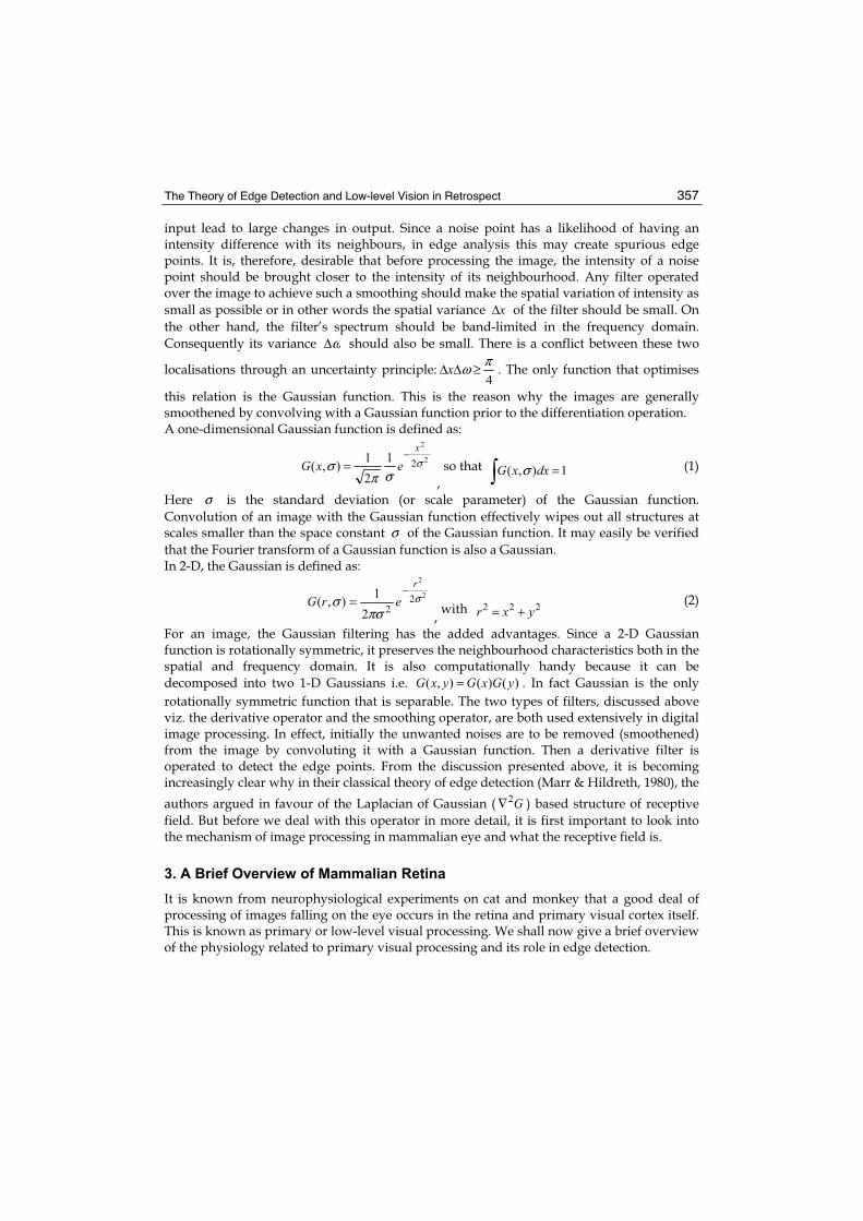
By combining the above two kernels, we get the omnidirectional operator corresponding to 2222 yx ∂∂+∂∂ :

Convoluting any intensity array u with this operator and combining the result linearly with u as has been proposed by Mach in Equation (5), is the same as convolving u with the filter mask given below:

Let us now convolve the Mach band image shown in Fig. 6 with this final mask. We find that the edges at each transition have become enhanced by a mechanism where new bands have been formed clearly separating each gray level from the other (Fig. 7a). To demonstrate that this again is not mere illusion, we draw a horizontal line profile through this convolved image to find undershoots and overshoots at each step transition that bears resemblance to our illusive perception of the original image whose line scan is in contrast simply a staircase function (Fig. 6b). So we understand what prompted Mach to propose the Laplacian operation as a model for spatial filtering in the retina and as is apparent from this mask, it is essentially excitatory-inhibitory in character, which also Mach claimed. Since we have already defined image edges as sharp changes in gray levels, therefore we may conclude from these observations that any image convoluted with the omnidirectional Laplacian mask will show pronounced Mach band effect at each edge of the filtered image. In other words, the edges will all be enhanced due to the effect of such a kernel being operated on any image, since new Mach bands will be created that would serve to clearly distinguish

-1 0 -1

0 4 0

-1 0 -1

-1 -1 -1

-1 8 -1

-1 -1 -1

-1 -1 -1

-1 9 -1

-1 -1 -1

Vision Systems - Segmentation and Pattern Recognition 364

one gray level from another. Edge enhancement by such a mechanism has been shown in Fig. 8. The resultant images clearly show an increase in the level of sharpness compared to the original images. The reason behind such sharpening is that the bright Mach bands around dark regions and the dark ones around lighter regions, apart from being illusions, also play a crucial role in image processing. They actually represent a mechanism of lateral inhibition or the contrast-sensitivity in the eye that enables one to clearly isolate an object

Fig. 7 (a) The effect of convoluting the Mach band image in Fig. 6a with the omnidirectional Laplacian mask clearly shows that new bands have actually been formed clearly separating each gray level from the other (b) This becomes obvious if we draw a horizontal line profile through the convoluted image, that shows the new bands as undershoots and overshoots at each step of the staircase shown in Fig. 6b. In other words a mimetic of the illusory perception of Fig. 6a, has thus been reproduced.

(a)

(b)

The Theory of Edge Detection and Low-level Vision in Retrospect 365

Fig. 8 Result of convoluting two bench-mark images in (a) and (c) with the omnidirectional discrete Laplacian mask has been shown in (b) and (d).

from its background, thus helping in image sharpening. As already mentioned, the polarities in the discrete mask resemble the antagonistic centre-surround receptive field structure shown in Fig. 4. Also, being an orientation independent operator, this mask naturally forms the Mach bands in all directions in an image, thus enhancing the images from objects of any arbitrary shape. What effectively gets sharpened in the process, are the edges in the images. This phenomenon, in fact, mystified Mach’s viewpoint about illusion and reality, which finally led him to construct the unscientific philosophy of empirio-criticism.

5. The Non-classical Receptive Field and Low-level Vision in Retrospect

When Marr and Hildreth (Marr & Hildreth, 1980) claimed the equivalence of LoG and DoG for a particular scale ratio between the two Gaussians, they could not provide any strong theoretical basis for the equivalence. That basis was provided much later in a paper by Ma and Li (Ma & Li, 1998), wherein they proved from very general consideration that any derivative filter of a smooth function could be expressed as a linear combination of the smooth function at different scale parameters. Ma and Li have shown that any kth2 order

(a) (b)

(c) (d)

Vision Systems - Segmentation and Pattern Recognition 366

derivative filter can be designed as the weighted sum of any )1( +k even functions, every function having the same kernel, but different scales. Also thk )12( + order derivative filter can be designed as the weighted sum of )1( +k odd functions of different scales. In the present chapter our discussion, with respect to non-classical receptive field will be confined only within even order derivative filters because we have chosen to construct filters at different scales by using two-dimensional Gaussian function, which happens to be an even function.But first, it would be appropriate to introduce the concept of non-classical receptive field of retinal ganglion cells. The concept of a centre-surround antagonistic receptive field of retinal ganglion cell, as we have already discussed, evolved on one hand, from Mach’s earlier studies in psychophysics and on the other from the later experiments dealing with the neurophysiology of retina. The DOG or LOG models merely follow this studies. Some experimental observations, however are strongly indicative of some necessary modification to this concept of “classical receptive field”. From such experiments from seventies onwards of the last century, it was observed that there are many photoreceptor cells outside the classical receptive field, that are capable of modulating the behaviour of the ganglion cells. Presently, there is practically no doubt that the actual receptive field of a ganglion cell is much widely spread than that depicted by the classical picture and that such an extended surround actually disinhibits the response of the classical receptive field. Such a non-classical receptive field containing non-linear sub-units is shown in Fig. 9, following a recent work (Passaglia et al., 2001), where it is conjectured that the mean increasing and mean decreasing units would remain either active or inactive depending on the desired task of the retina.Although the modulation of the ganglion cells by the non-classical receptive field is probably nonlinear in nature, yet some of the effects of the non-classical receptive field may be emulated by modeling the corresponding response bahaviour simply as a linear combination of three or more zero-mean Gaussians at different scales. The narrower two of

Fig. 9 The non-classical receptive field of retinal ganglion cells is characterised by an extended disinhibitory surround beyond the classical receptive field

The Theory of Edge Detection and Low-level Vision in Retrospect 367

these Gaussians may represent the classical center and the classical antagonistic surround while the non-classical extended disinhibitory surround mostly contributed by the amacrine cells in the inner plexiform layer of the retina may be represented by the wider Gaussians. Since, according to Ma and Li (Ma & Li, 1998), such a linear combination of Gaussians could be expressed as equivalent to higher order derivatives, therefore from such an argument it can been shown, that the non-classical receptive field of retinal ganglion cells can be modeled by a fourth or sixth order rotationally symmetric derivative of Gaussian, that is by G4∇ (the Bi-Laplacian or Bi-harmonic of Gaussian) or G6∇ (the tri-Laplacian of Gaussian).

The detailed expressions are given in the sub-section 5.1 for the one-dimensional case, where it has also been shown that one could express G4∇ as 1GDoG + where 1G is the widest Gaussian representing a disinhibitory surround beyond the classical receptive field or in other words the mean-increasing sub-units in Fig. 9. Similarly, G6∇ can be expressed as 21 GGDoG −+ , where 2G is another wide Gaussian representing the mean-decreasing sub-units in the same figure.

5.1 A Simple Model for the Non-classical Receptive Field Structure

If the positive sub-units of the non-classical receptive field are primarily considered, then in one dimension, following Ma and Li, one can construct a fourth order derivative filter as a linear combination of three Gaussians. For this, let us define a function kh2 using the primitive Gaussian filter ),( σxg as:

== j

k

j j

jk

xgxhσσ

α

0

2 )( , where 2

2

2

2

1 σπσ

x

exg−

= (6)

Here jα ’s are the weight functions. Ma & Li showed that kh2 is a ( )k2 -th order derivative filter if the jα ’s satisfy the following equations :

( )kg

kkk

kkk

kk

k

mk2,

2222

211

200

2222

211

200

210

!2......................

0.....................

0....................

=++++

=++++

=++++

σασασασα

σασασασα

αααα

and if the matrix σM

=

kk

kk

kM

221

20

221

20

...

......

...

1...11

σσσ

σσσσ (7)

is not singular. Here kgm 2, is the thk)2( order moment of the function ( )xg .Thus, for second order derivative, taking 1=k , one gets

Vision Systems - Segmentation and Pattern Recognition 368

( ) −=1100

02

11

σσσσα xgxgxh (8)

Here 0α is a ratio of scale parameters. For a scale ratio t , i.e. if σσ =1 and σσ t=0

( )( )

( ) −=−−

2

2

2

2

2202

2

1

2

1 σσ

πσπσα

xtx

eet

xh (9)

Similarly, for fourth order derivative filter, let us define a function

( ) ++=22

211

100

04111

σσα

σσα

σσα xgxgxgxh (10)

where 10 ,αα and 2α satisfy the following equations

4,

422

411

400

222

211

200

210

!4

0

0

gm=++

=++

=++

σασασα

σασασα

ααα

where, ( )dxxgxmg

∞

∞−

= 44, (11)

Solving these equations, we get:

( )( )

( )20212

20

221

21

220

σσα

σσα

σσα

−=

−−=

−=

k

k

k

where ( )( )( )2122

20

21

20

224,

124

σσσσσσ −−−=

gmk (12)

In this case, for the two scale ratios t and p , i.e. if σσ =2 , σσ t=1 and σσ p=0 , then:

( )( )

( )2222

221

220

1

1

ptk

pk

tk

−=

−−=

−=

σα

σα

σα

(13)

If we take a look at the final values of the three coefficients, 10 ,αα and 2α as given by Equation (13), we find that a fourth order derivative filter as given in Equation (10) is

The Theory of Edge Detection and Low-level Vision in Retrospect 369

essentially a non-classical 1GDoG + model as mentioned in the previous section. Moreover, experimental observations on non-classical receptive fields (Passaglia et al., 2001), indicate that the central region is much smaller than the extended surround, or in other words 0σ is negligible in comparison to 2σ . Based on these, we can consider the ratio 20 :σσ to be very small and hence apply a condition 0→p in Equation (13). Then using Equation (10), we arrive at:

( )→σ,4 xh ( )/2 ,σxmh ( )//

2 ,σxh+ (14)

where, /σ and //σ are two arbitrary scales and m is an amplitude scale factor and ( )xh2 is given by Equation (9). In the same way if we incorporate the negative sub-units of non-classical receptive field, then following the same procedure:

+++=33

3

22

2

11

1

00

06 )(

σσα

σσα

σσα

σσα xgxgxgxgxh (15)

Here

( )( )( )( )( )( )

( )( )( )( )( )( )2222226

3

222262

222261

222260

11

11

11

rpptrtk

prrpk

rttrk

tpptk

−−−=

−−−−=

−−−=

−−−−=

σα

σα

σα

σα

where σσσσσσσσ rpt ==== 0123 ,,, (16)

If we again take a look at the final values of the four coefficients, 10 ,αα , 2α and 3α , we find that the corresponding expression matches the 21 GGDoG −+ model described in the previous section. Then once again following the same procedure described above we assume 30 :σσ to be very small and apply a condition 0→r in Equation (16). Putting these values in Equation (15), after some algebraic manipulation, we finally arrive at:

( )→σ,6 xh ( )/2 ,σxmh + ( )//

2 ,σxnh ( )///2 ,σxh+ (17)

Then applying Equation (14) in Equation (17), we get:

( )→σ,6 xh ( )/2 ,σxmh ( )//

4 ,σxh+ (18)

Here ////// ,, σσσ are all arbitrary and hence do not represent any particular scale at any stage of the derivation. So in two dimensions:

)()()( 426 rGrGmrG ∇+∇=∇ ,

where −+−=∇2

2

4

4

2

2

6

4

2exp18

2

1)(

σσσπσrrrrG (19)

Vision Systems - Segmentation and Pattern Recognition 370

Any of these equations viz. Equation (10), (14), (15) or (19) may be considered to be our proposed model for non-classical receptive field, which means the receptive field will not be represented by LOG only whose equivalent physiological model is given by Equation (8), but rather by a linear combination of even order isotropic Gaussian derivatives. So the advantage of economy of computation that was applicable for LOG remains valid, while at the same time apart from the scale of the Gaussians, the factor m can also play a role in visual information processing at low level. To understand this more clearly we have to again resort to a corresponding receptive field like spatial organization as before for such a mathematical function and see whether it also reflects the disinhibitory extended surround in such a form of representation.

5.2 Derivation of a Kernel for the Non-classical Receptive Field

First of all we discuss on the construction of a computationally handy kernel for the 4∇

operator following the methodology of construction of the convolution matrix for the 2∇operator, using finite difference approximation as discussed in section 4. Clearly,

4∇ = 22.∇∇

=∂∂

∂∂

∂∂

∂∂

2

2

2

2

2

2

2

2

+.+yxyx

So, 4∇ = 24

4

4

4

+∂∂+

∂∂

yx 2

2

x∂∂

2

2

y∂∂ (20)

Utilising the finite difference approximation of the fourth order partial derivative, the kernel for 44 x∂∂ in discrete domain can be represented by the kernel:

By transposing this kernel we may construct the corresponding vector for 44 y∂∂ , add these, so that we get the corresponding matrix for a linear combination of these two terms,

i.e. for 4

4

4

4

yx ∂∂+

∂∂ :

0 0 1 0 0 0 0 -4 0 0 1 -4 12 -4 1 0 0 -4 0 0 0 0 1 0 0

Using the expressions for 22 x∂∂ and 22 y∂∂ in section 4 we may arrive at a 55× matrix

for2

2

2

2

yx ∂∂

∂∂ :

≡∂∂ 44 x 1 -4 6 -4 1

The Theory of Edge Detection and Low-level Vision in Retrospect 371

Then from equation (20), we arrive at the following kernel for the Bi-Laplacian operator:

As in the case of deriving the Laplacian kernel the diagonal directions are now incorporated by taking the co-ordinates along the diagonals through a 4π radian rotation. The new kernel thus obtained is then added as before, to the above kernel so that we arrive at the mask:

But, unlike the Laplacian, this being a 55× mask, the asymmetry still remains and in order to arrive at an omnidirectional mask for the isotropic 4∇ operator, we apply another 8πradian rotation so that we may also incorporate the off-diagonal elements. Then once again adding the new kernel thus obtained to the above mask, the final form that the Bi-Laplacian mask assumes is:

0 0 0 0 0 0 1 -2 1 0 0 -2 4 -2 0 0 1 -2 1 0 0 0 0 0 0

0 0 1 0 0 0 2 -8 2 0 1 -8 20 -8 1 0 2 -8 2 0 0 0 1 0 0

1 0 1 0 1

0 -6 -6 -6 0

1 -6 40 -6 1

0 -6 -6 -6 0

1 0 1 0 1

1 1 1 1 1

1 -12 -12 -12 1

1 -12 80 -12 1

1 -12 -12 -12 1

1 1 1 1 1

Vision Systems - Segmentation and Pattern Recognition 372

Fig. 10 The two benchmark images (a) and (d) used in section 4, have been enhanced with the discrete Laplacian mask in (b) and (e) and by the derived digital mask in (c) and (f).

Since, the non-classical receptive field has been modelled by Equation (19) in the previous sub-section, therefore we shall now try to arrive at a new omnidirectional mask that is comparable to the omnidirectional Laplacian mask and at the same time whose spatial organization reflects the disinhibitory extended surround as an added feature to the lateral inhibition evident in the spatial organization of the Laplacian mask. We show below one such possiblity. We choose the value of m in Equation (19), so that if we combine the Laplacian and the Bi-Laplacian masks by a ratio of 1:9 , we arrive at such a new 55× discrete filter comparable in simplicity to the 33× Laplacian mask:

Correspondingly, by including the original intensity distribution to such a derivative opeartor, as a modification to the proposal of Mach given by Equation (5), we get a new spatial organization for the non-classical receptive field that includes disinhibitory inputs

-1 -1 -1 -1 -1

-1 3 3 3 -1

-1 3 -8 3 -1

-1 3 3 3 -1

-1 -1 -1 -1 -1

(a) (b) (c)

(d) (e) (f)

The Theory of Edge Detection and Low-level Vision in Retrospect 373

from the surround extended from the classical excitatory-inhibitory organization of receptive field:

This is the new omnidirectional mask whose performance in enhancing edges, we can now compare with the omnidirectional Laplacian mask. From visual inspection (Fig. 10) it is clear that this new discrete filter derived from a combination of Laplacian and Bi-Laplacian, indeed performs better compared to the discrete Laplacian mask. The Mach bands have been further enhanced by the new discrete filter as compared to the discrete Laplacian filter, which leads to better segregation of objects from background and hence better edge enhancement. The incorporation of disinhibition has therefore further improved edge enhancement.

5.3 Explanation of Complex Brightness-contrast Illusions

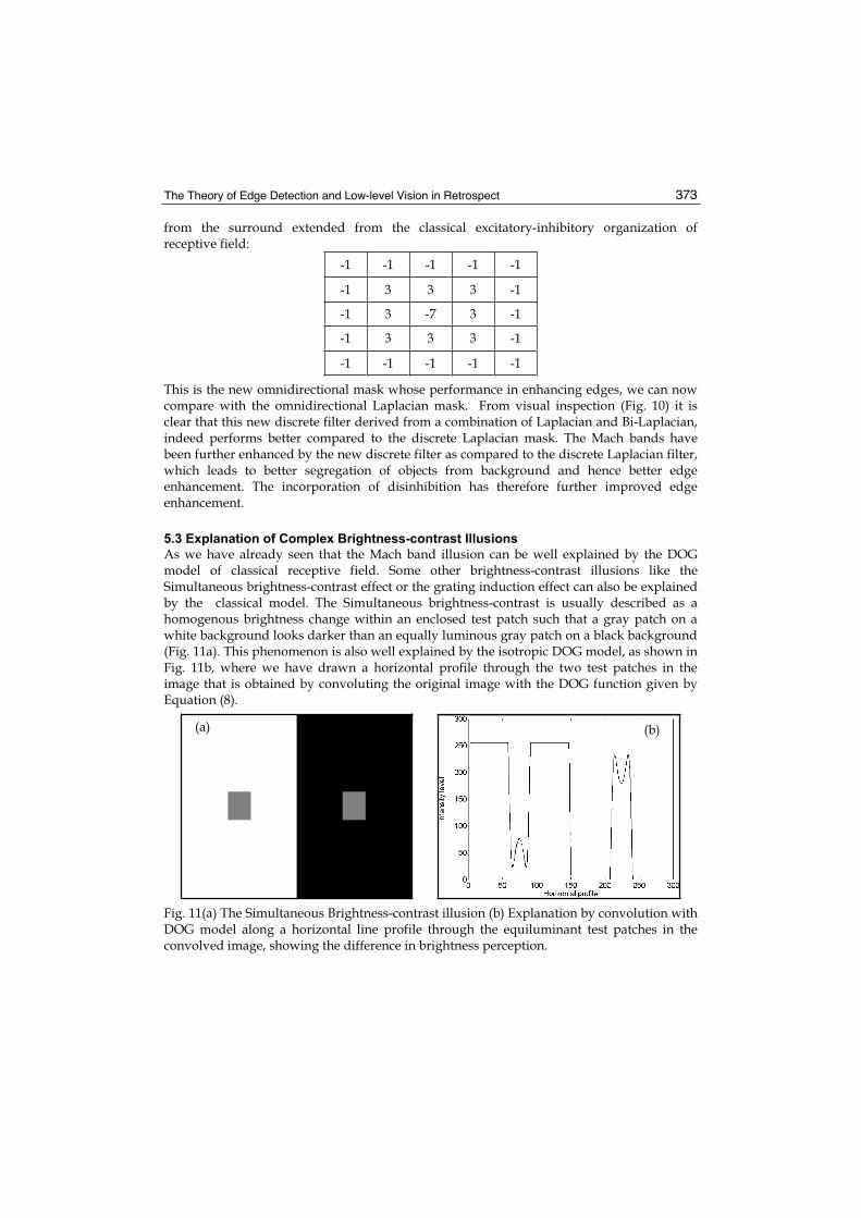
As we have already seen that the Mach band illusion can be well explained by the DOG model of classical receptive field. Some other brightness-contrast illusions like the Simultaneous brightness-contrast effect or the grating induction effect can also be explained by the classical model. The Simultaneous brightness-contrast is usually described as a homogenous brightness change within an enclosed test patch such that a gray patch on a white background looks darker than an equally luminous gray patch on a black background (Fig. 11a). This phenomenon is also well explained by the isotropic DOG model, as shown in Fig. 11b, where we have drawn a horizontal profile through the two test patches in the image that is obtained by convoluting the original image with the DOG function given by Equation (8).

Fig. 11(a) The Simultaneous Brightness-contrast illusion (b) Explanation by convolution with DOG model along a horizontal line profile through the equiluminant test patches in the convolved image, showing the difference in brightness perception.

-1 -1 -1 -1 -1

-1 3 3 3 -1

-1 3 -7 3 -1

-1 3 3 3 -1

-1 -1 -1 -1 -1

(a) (b)

Vision Systems - Segmentation and Pattern Recognition 374

Grating Induction, on the other hand, refers to a periodic apparent contrast induced in uniform fields by adjacent gratings. This image displays a brightness effect that produces a spatial brightness variation (a grating) in an extended test patch (Fig. 12a). This effect can

Fig. 12 (a) The Grating Induction illusion. (b) Explanation by convolving the image with DOG model along two horizontal line profiles, one through the constant intensity test patch (solid line) and one through the grating (dotted line) in the convolved image.

Fig. 13 (a) The White effect illusion. (b) Attempted explanation with conventional isotropic DOG function along a horizontal line profile through the equiluminant gray segments in convolved image, gives results in brightness perception contrary to our visual sensation.

also be similarly explained by the DOG model as has been shown in Fig. 12b, by drawing two horizontal profiles one through the test patch and the other through the grating. However, many other brightness-contrast illusions like the White effect and the checkerboard illusion cannot be explained using the classical DOG model. In the White effect, for example in a square grating of black and white bars, if identical gray segments are used to replace part of the black bars and also part of the white bars, then the former gray segments look brighter than the later (Fig. 13a). Conventional isotropic DOG filters, fail to simulate this illusion and produce results contrary to our perception (Fig. 13b). The effect is specifically interesting because it does not depend on the amount of dark or white border in the vicinity of the test patch. True, that the effect may be generated if lateral inhibition shows directional properties i.e. inhibition is supposed to be stronger along the bars than

(a) (b)

(a) (b)

The Theory of Edge Detection and Low-level Vision in Retrospect 375

across them, but such a supposed anisotropy in lateral inhibition is not observed in White’s effect on checkerboard (Fig. 14a), a symmetric image that cannot be explained with the

Fig. 14 (a) The checkerboard illusion. The horizontal line profiles through the two test patches of the image obtained after convolution with DOG model. From the horizontal line profiles it is clear that the test patch on the left in darker neighbourhood (solid line representation) appears brighter compared to the one on right (dotted line representation), which is opposite to our perceptual experience.

Fig. 15 Explanation of the White effect illusion by convolving the image with the

1GDoG + model which produces results that match our brightness perception.

isotropic DOG model as well (Fig. 14b). Gestalt theorists believe that White effect can be understood only in terms of perception at a higher level and hence such illusions are often considered as more complex brightness-contrast phenomena that fall beyond the scope of low-level vision. Thus to probe whether the explanation of the White effects could have a basis in the retinal physiology, it would indeed be tempting to use the model of non-classical receptive field in the simulation of the White effects (Ghosh et al., 2006). We find that the White effect illusions, for both the anisotropic and isotropic (checkerboard) cases, where the DOG model failed completely, can be faithfully explained by convoluting the images with the function given by Equation (10), i.e. by the non-classical 1GDoG + model. This has been shown in Fig. 15 and Fig. 16.

(a) (b)

(a) (b)

Vision Systems - Segmentation and Pattern Recognition 376

Fig. 16 Explanation of the checkerboard illusion by convolving the image with the 1GDoG + model producing results similar to our brightness perception.

5.4 A Possible Explanation of the Filling-in Mechanism in Retinal Blind Spot

It is well-known that human beings have a blind spot in each of their eyes. This blind spot is nothing but the area of the visual space that corresponds to the area on the retina, where all the optic nerves emanate from the retina (Fig. 17). It is called a blind spot because at this corresponding position, the retina is devoid of any rod or cone cell for receiving visual information. The area in visual space, marking the blind spot for one eye, is covered by the retina of the other eye. Curiously however, even in monocular vision, no hole is perceived in the visual field. This phenomenon is referred to as “filling-in” of the blind spot. According to many vision scientists (Ramachandran, 1992), the blind spot is not ignored, but “filling-in” is continually performed by the human visual system, constructing a representation based on the visual stimulation of the area surrounding the blind spot. Such an information processing based approach bears resemblance to David Marr’s (Marr, 1982) computational investigation of human representation and processing of visual signals. Marr speculated that the computational theory of vision should cover three different possible phases in information processing: a) an early primal sketch of which “raw primal sketch” or detection of edges is the fundamental step, b) surface interpolation or the filling-in of colour and texture leading to the “two-and-half dimensional sketch” and c) object reconstruction and classification being the final step. So according to this theory, interpolation is an integral part of image retrieval in vision. In a bid to understand the process of interpolation, Ramachandran has performed some psychophysical experiments to come up with very interesting results on the “filling-in” of blind spots. He has shown that this “filling-in” process must occur as early as the detection of edges in the simple cells of primary visual cortex. However such interpolation cannot be explained by the classical DOG function of low-level receptive field. For any kernel h(x) to qualify for an interpolator it must obey the following conditions:

=≡=≡

3,2,1,0)(

0,1)(

xxhxxh

(21)

(a) (b)

The Theory of Edge Detection and Low-level Vision in Retrospect 377

Fig. 17 A rough schematic of the eye that demonstrates the existence of the blind spot in the retina of each of the eyes from where the optic nerves emerge out towards the brain.

Secondly, it must also comply with the condition for dc-constancy, which implies that the sum of the samples of the interpolator should be unity for any displacement 10 <≤ d i.e.:

1)( ≡+∞

−∞=

dchc

(22)

Functions that do not fulfill Equations (21) and (22) are called ‘approximators’ and do not represent the ideal interpolators. The ideal interpolation function for convolution is the sinc function:

)(sin)sin(

)( xcxxxh ideal ==

ππ

It has an infinite support having innumerable zero-crossings. This needs to be truncated to obtain a finite support interpolation kernel. From this consideration, the DOG response function of the classical receptive field given in Fig. 18a, should be an unlikely contender for performing the task of interpolation. This is because by comparing the kernel, with the second condition in Equation (21), we easily realize that this interpolator can have only one zero-crossing at 1=x , and can therefore at best mimic the highly truncated sinc interpolator within the interval 11 ≤≤− x . It will thus behave poorly in frequency domain and invariably produce erroneous results, unlike our almost perfect visual experience in the filling-in of blind spot. So as in the case of the complex brightness-contrast illusions, we again feel

Vision Systems - Segmentation and Pattern Recognition 378

Fig. 18 (a) The DOG kernel in one dimension can have only one zero-crossing at 1=x . It is therefore not possible to design a good interpolator with such a function. (b) The

21 GGDoG −+ kernel is being shown here as a near ideal interpolator with 3 zero-crossings at 3,2,1=x and 1)( =xh at 0=x

tempted to investigate if our model of non-classical receptive field can suit the purpose of near ideal interpolation in low-level vision. For this we use Equation (15) as the convolution function for interpolation or in other words the 21 GGDoG −+ model of non-classical receptive field. From Fig. 18b we find that four zero-mean Gaussians representing the non-classical receptive field, can produce 3 zero-crossings at 3,2,1=x (Sarkar et al., 2005). This kernel, it is easy to verify will have excellent frequency domain as well as dc-constancy behaviour (Fig. 19) and is therefore a reasonably good contender for performing near ideal interpolation in the blind spot of the retina. Hence the proposal, put forward from the observations on the psychophysical experiments (Ramachandran, 1992) that information

(a)

(b)(b)

The Theory of Edge Detection and Low-level Vision in Retrospect 379

corresponding to the blind-spot can be interpolated out at an early stage of visual processing, is also vindicated, since the interpolation function used here is a low-level receptive field model only.

6. Conclusion

The theory of edge detection and the treatise on low-level vision presented in this chapter in the light of the non-classical receptive field of retinal ganglion cells is a straightforward continuation of the approach of David Marr and his group. The appeal of the present approach lies in its simplicity and easy implementation, although it should be kept in mind that no non-linear model of the extended surround has been proposed here, which could be an interesting direction of future work. Potential applications of the algorithm will include apart from areas of general edge enhancement, designing new robust visual capturing or

Fig. 19 Representative curves for the interpolation kernel constructed using the 21 GGDoG −+ function (a) Fourier spectrum of the kernel and (b) dc constancy bahaviour of the kernel

(b)

(a)

Vision Systems - Segmentation and Pattern Recognition 380

or display systems and automatic detection and correction of perceived incoherence of luminance in video display panels, where accurate perception of intensity level is critical. Such applications will be important particularly in mission-critical domains such as aircraft display panel design. Also, the concept of disinhibition introduced into the low-level receptive field structure, can be extended in future to higher brain functions such as categorization and memory. It is possible that a close analysis of cortical horizontal connections and their physiology under the disinhibition framework can provide us with new insights on their functions. This in turn will allow us to apply the general concept of disinhibition in advanced intelligent systems, firmly based on biological observations.

7. References

Barlow, H. B. (1953). Summation and inhibition in the frog’s retina. Journal of Physiology (London), 119, 69-88

Helmholtz, H. von (1867/1925). Treatise on Physiological Optics, (from Third German Edition, Trans.), Dover Publications, New York

Ghosh, K., Sarkar, S. & Bhaumik, K. (2006) A possible explanation of the low-level brightness-contrast illusions in the light of an extended classical receptive field model of retinal ganglion cells. Biological Cybernetics, 94, 89-96.

Ma, S. D. & Li, B. (1998). Derivative computation by multiscale filters. Image and Vision Computing, 16, 43-53

Mach, E. (1865/1965). On the effect of the spatial distribution of the light stimulus on the retina, Trans. In: Mach Bands: Quantitative Studies on Neural Networks in the Retina, F. Ratliff (Ed.), Holden-Day, San Francisco

Marr, D. (1982). Vision, W. H. Freeman and Company, ISBN 0-7167-1567-8, New York Marr, D. & Hildreth, E. (1980). Theory of edge detection. Proceedings of the Royal Society of

London B, 207, 187-217 Passaglia, C.L., Enroth-Cugell, C. & Troy, J. B. (2001). Effects of remote stimulation on the

mean firing rate of cat retinal ganglion cell. Journal of Neuroscience, 21, 5794-5803 Ramachandran, V. S. (1992). Blind spots. Scientific American, 266 (5), 44-49 Sarkar, S., Ghosh, K. & Bhaumik, K. (2005). A weighted sum of multi-scale Gaussians

generates new near ideal interpolation functions, Proceedings of 27th Annual International Conference of the IEEE Engineering in Medicine and Biology Society, pp. 6387-6390, ISBN: 0-7803-8741-4, Shanghai, China, September, 2005, IEEE Press, New Jersey.