ADVANCEMENTS IN NONCLASSICAL GAS DYNAMICS
291
ADVANCEMENTS IN NONCLASSICAL GAS DYNAMICS Proefschrift ter verkrijging van de graad van doctor aan de Technische Universiteit Delft, op gezag van de Rector Magnificus prof. dr. ir. J. T. Fokkema, voorzitter van het College voor Promoties in het openbaar te verdedigen op dinsdag 12 mei 2009 om 15:00 uur door Nawin Ryan NANNAN werktuigkundig ingenieur geboren te Paramaribo, Suriname
-
Upload
khangminh22 -
Category
Documents
-
view
2 -
download
0
Transcript of ADVANCEMENTS IN NONCLASSICAL GAS DYNAMICS

ADVANCEMENTS IN NONCLASSICAL GAS DYNAMICS
Proefschrift
ter verkrijging van de graad van doctoraan de Technische Universiteit Delft,
op gezag van de Rector Magnificus prof. dr. ir. J. T. Fokkema,voorzitter van het College voor Promoties
in het openbaar te verdedigen op dinsdag 12 mei 2009 om 15:00 uur
door
Nawin Ryan NANNAN
werktuigkundig ingenieurgeboren te Paramaribo, Suriname

Dit proefschrift is goedgekeurd door de promotor:
Prof. ir. J. P. van Buijtenen
en de copromotor
Dr. P. Colonna
Samenstelling promotiecommissie:
Rector Magnificus voorzitterProf. ir. J. P. van Buijtenen Technische Universiteit Delft, promotorDr. P. Colonna Technische Universiteit Delft, copromotorProf. dr. F. Scarano Technische Universiteit DelftProf. dr. ir. M. E. H. van Dongen Technische Universiteit EindhovenO.Univ.Prof. Dipl.-Ing. Dr.techn. Technische Universitat Wien,A. Kluwick OostenrijkProf. dr. ir. C. J. Peters The Petroleum Institute, V.A.E.Dr. S. Rebay Universita degli Studi di Brescia, ItalieProf. dr. G. J. Witkamp Technische Universiteit Delft, reservelid
This research is supported by the Dutch Technology Foundation STW, appliedscience division of NWO and the Technology Program of the Ministry of Eco-nomic Affairs, the Netherlands, grant number DSF.6573.
ISBN 978-90-9024285-9
Copyright c© by N. R. Nannan1
All rights reserved. No part of the material protected by this copyright noticemay be reproduced or utilized in any form or by any means, electronic or me-chanical, including photocopying, recording or by any information storage andretrieval system, without the prior permission of the author.
Front cover design by Andrea Lucchini and Martina Fantini.
1Author email: [email protected]


SummaryAdvancements in nonclassical gas dynamics
Shock waves can be formed in all states of matter, be it in the single- or multi-phase condition, when the substance is subjected to a rapid change of state,e.g., a sudden pressure or temperature variation. In the case of shock waves ingases, because of the fact that the developed theory is often based on the ideal-gas thermodynamic model, it is commonly accepted (by some even nowadaysconsidered as an irreconcilable truth) that shock waves can be only of the com-pressive type, i.e., in the direction of flow, the gas experiences an abrupt increaseof pressure whilst undergoing a supersonic-to-subsonic transition. Although ithas been known since the late 1940s due to the works of Bethe and Zel’dovichand collaborators that it is in principle possible, from a theoretical point of view,to deliberately create expansion shock waves, provided that the correct sub-stance and initial states are chosen, it was only until the early 1970s that theadmissibility of expansion shock waves, i.e., shock waves featuring a transitionsuch that in the direction of flow, the single-phase fluid experiences an abruptpressure decrease, was accepted. The caloric property that is key in determin-ing the nature of shock waves is referred to as the fundamental derivative of gasdynamics, Γ, of which the implications of its behavior were studied in detail byThompson and coworkers. In honor of the above-mentioned researchers, com-pounds that can admit expansion shock waves due to the existence of an em-bedded region of Γ < 0 in the dense-gas single-phase thermodynamic regimeare referred to as BZT fluids, as first proposed by Cramer.
Further progress in the field of compressible fluid dynamics, specifically re-lated to the study of nonclassical gas dynamic phenomena, as are for exampleexpansion shock waves, necessitates the availability of experimental evidence.The motivation of this research stems from: i) the need of such an experimentto demonstrate the existence of nonclassical gas-dynamic phenomena in densegases of molecularly complex fluids, the most intriguing of which is the theo-retical admissibility of expansion shock waves, specifically because of the fail-ure or ambiguity of previous two experiments (one in the early 1980s and onein the late 1990s), and ii) the fact that nonclassical gas-dynamic phenomenacan be exploited in technical applications operating in the dense-gas regime orin transonic or supersonic conditions. One such example is the utilization ofnonclassical gas-dynamic phenomena in small, decentralized energy conver-
i

sion systems operating according to the Rankine principle.The research documented herein aims to develop, design, build and com-
mission an experimental facility which can be used to generate and study non-classical expansion shock waves in molecularly complex substances classifyingas potential BZT candidates. Secondarily, the facility that is to be built should bemodular and flexible in its design and should therefore allow for studying bothclassical and nonclassical dense-gas flows. Cascading from the main goal, rele-vant theory has been developed. The results of these investigations are also use-ful/necessary for validating the proprietary software package for gas-dynamicsimulations using real-gas properties.
To achieve the(se) goal(s), it is required to formulate relevant research ques-tions, e.g., what is necessary from a physical perspective to give rise to the for-mation of rarefaction shock waves?, what is currently known about rarefactionshock waves in particular and nonclassical gas dynamics in general?, is it tech-nically and economically feasible to build a facility to create and to investigatenonclassical gas-dynamic effects, how should this be done and what are theconstraints?, etc. Answering these questions mandates a thorough but concisereview of the theory of nonclassical gas dynamics, as documented in Chap. 2.Secondly, as was indicated, the study of Bethe has shown that certain nonclas-sical gas-dynamic phenomena are only permissible due to, among other things,the molecular complexity of the compound. That is, the fluid should have suf-ficient capability to store dynamic energy. Therefore, Chap. 3 focusses exclu-sively on the thermodynamic description of the test fluid from both a theo-retical, semi-empirical and experimental viewpoint. Here, because of their fa-vorable thermophysical characteristics, e.g., low toxicity, lubricating properties,etc., substances within the dimethylsiloxanes family are considered. Further-more, the prediction of Γ as well as the identification of BZT-candidate fluidswithin the dimethylsiloxanes family is treated in Chap. 4. It is found, for exam-ple, that if highly accurate thermodynamic equations of state are available, Γcan be calculated with a degree of uncertainty that is suitable for the design andanalysis of dense-gas applications, and, that for molecularly complex fluids, it ispossible to achieve a comparatively higher level of accuracy in the estimation ofΓ with respect to molecularly simpler fluids, if experimental data are available.For well-measured substances, technical multiparameter equations of state canbe developed and the use of these can result in an appreciable improvementwith respect to the uncertainty of the estimation of Γ. Additionally, the in-vestigation of the vapor-liquid critical region of a single-component fluid hasyielded the potential existence of nonclassical expansion-condensation shockwaves in a wide class of substances not specifically classifying as BZT fluids,e.g., methane, carbon dioxide. Once the more fundamental aspects have beenconsidered, Chap. 5 discusses various methods to experimentally demonstratethe existence of unconventional expansion shock waves in BZT fluids. The out-come of this study is that it is both theoretically and technically possible to cre-ate an unsteady nonclassical expansion shock wave in a polyatomic substance
ii

classifying as a BZT fluid, namely dodecamethylcyclohexasiloxane. An assess-ment based on arguments for and against each identified method, taking as-pects like reproducibility and repeatability of the experiment, costs, safety con-cerns, etc. into account, has resulted in the design and building of the FlexibleAsymmetric Shock Tube (FAST) – a unique facility for high-temperature gas-dynamic experiments in organic fluids – equipped with a novel, custom-madefast-opening valve. The experiment conducted with the FAST aims at creating aso-called maximum-Mach expansion shock wave that is detected using four dy-namic pressure instruments and a time-of-flight technique. The detailed designof the FAST is presented in Chap. 6. During the commissioning phase, discussedin Chap. 7, all pieces of equipment have been tested and the temperature con-trol system has been thoroughly scrutinized. Also tests related to the intendedexperiment have been done with air and the time-of-flight technique has beentested. Alas, after suffering much delay (more than 11/2 year) it is postponed tothe follow-up of this project to provide experimental evidence of a rarefactionshock wave in dodecamethylcyclohexasiloxane. Chapter 8 gives concluding re-marks and recommendations for future work.
Nawin Ryan Nannan, April 8, 2009
iii


SamenvattingVorderingen in de niet-klassieke
gasdynamica
Indien een medium, zij het in de een- of meerfase toestand, wordt onderwor-pen aan een snelle verandering van bijvoorbeeld druk of temperatuur, kan dezeresulteren in de vorming van een of meerdere schokgolven. In het geval dat hetschokgolven in gassen betreft, wordt vaak impliciet verondersteld, mede van-wege het feit dat de ontwikkelde theorie over schokvorming is toegespitst opideale gassen, dat in de richting van de stroming, het gasvormig medium si-multaan een abrupte compressie alsmede een supersone–subsone transitie on-dergaat. Alhoewel het sinds de late jaren 40 bekend is uit de werken van Betheen Zeldo’vich en medewerkers dat vanuit een theoretisch oogpunt, indien eengeschikte stof is gekozen, expansie schokgolven – deze zijn schokgolven waar-bij het medium een abrupte drukverlaging ondervindt bij het passeren van eenfront, terwijl simultaan een (super)sone–(sub)sone transitie plaatsvindt – kun-nen worden gegenereerd, heeft het tot de jaren 70 geduurd vooraleer dit werdgeaccepteerd. De aard van een schokgolf wordt vanuit een thermodynamischoogpunt bepaald door de fundamentele afgeleide der gasdynamica, Γ; gede-tailleerde studies betreffende de implicaties van het gedrag van Γ op compress-ibele stromingen zijn uitgevoerd mede door Thompson. Ter ere van de bijzon-dere bijdrage van Bethe, Zeldo’vich en Thompson aan de tak van de compress-ibele gasdynamica, worden stoffen die een thermodynamisch domein bezittenmet Γ < 0 in het verdichte damp gebied (dit is het domein nabij de damp-vloeistof kritieke toestand van een stof, rechts van en inclusief de verzadigdedamp lijn in een druk-specifiek volume, P -v, toestandsdiagram), en derhalveexpansie schokgolven kunnen handhaven, gerefereerd als BZT fluida. Het gas-dynamisch gedrag van compressibele media als gevolg van het feit dat een stofzulk een thermodynamisch domein beschikt, wordt beschouwd als zijnde niet-klassiek.
Verdere ontwikkelingen in de niet-klassieke gasdynamica (waartoe de zo-juist genoemde expansie schokgolven behoren) vergt experimenteel bewijs vanBZT effecten. De motivatie voor dit onderzoek stamt uit: i) de noodzaak omexperimenteel bewijs te leveren voor het bestaan van onconventionele, niet-klassieke gasdynamische fenomenen, dan wel de toelaatbaarheid van expansie
v

schokgolven, met name vanwege de discutabele resultaten van twee eerder uit-gevoerde experimenten (het eerste experiment dateert uit de jaren 80 en hettweede is uitgevoerd in de late jaren 90), en ii) het feit dat niet-klassieke gasdy-namische effecten kunnen worden geexploiteerd in processen welke plaatsvin-den in het verdichte damp gebied onder transsone of supersone condities. Eenvoorbeeld van zo een proces is de expansie van het werkmedium in de tur-bine van een mini- of microwarmtekracht unit. Zulke units werken volgens hetRankine cyclus en maken gebruik van een organisch stof en beoogde applicatieszullen worden ontwikkeld voor vermogens in de kWatt orde-grootte.
Het gedocumenteerde onderzoek richt zich op het ontwikkelen, ontwerpenen opzetten van een experimentele opstelling welke kan worden toegepast omin een moleculair complex organisch fluıdum, onconventionele expansie schok-golven te genereren en daar metingen aan te verrichten. Bijkomstig hieraan isdat de te bouwen opstelling modulair dient te zijn, zodat de opstelling flexibelis in haar gebruik. De resultaten van dit onderzoek zijn bovendien nodig voorhet valideren van de binnen de afdeling ontwikkelde CFD software programmawelke gebruik maakt van toestandsgrootheden van reele gassen.
Om de bovengenoemde doelstellingen te realiseren, is het nodig om juisteonderzoeksvragen te formuleren, bijvoorbeeld: wat is nodig vanuit een fysischperspectief om expansie schokgolven te creeren?, wat is thans bekend over ex-pansie schokgolven in het bijzonder en de niet-klassieke gasdynamica in hetalgemeen?, is het uberhaupt mogelijk, vanuit een technisch en economisch per-spectief, om een opstelling op te zetten waarmee niet-klassieke gasdynamischeeffecten kunnen worden bestudeerd, hoe dient zo een experiment uitgevoerdte worden en wat zijn de mogelijke beperkingen? Formulering van geschikteantwoorden op de laatstgenoemde vragen vergt, ten eerste, een grondige dochbeknopte beschouwing van de theorie, zoals gedocumenteerd in Hfdst. 2. Tentweede, zoals eerder was aangegeven, heeft de studie van Bethe aangetoonddat de toelaatbaarheid van expansie schokgolven onder andere wordt bepaalddoor de moleculaire complexiteit van een stof, met name, de capaciteit van hetmedium om dynamische energie inwendig op te slaan. Vandaar dat Hfdst. 3 pri-mair de nadruk legt op de thermodynamische beschrijving van het testmedium.Voor dit onderzoek zijn siloxaan olien geselecteerd, omdat deze stoffen vanuiteen experimenteel pespectief gunstige thermofysische eigenschappen bezitten,zoals lage toxiciteit, goede smeeringseigenschappen, enz. Verder is de bepal-ing van de numerieke waarde van Γ alsook de identificatie van zogenoemdeBZT media behandeld in Hfdst. 4. Uit de in Hfdst. 4 verrichtte studie blijktbijvoorbeeld dat, indien nauwkeurige toestandsvergelijking aanwezig zijn vooreen bepaalde stof, Γ kan worden uitgerekend met een nauwkeurigheid welkevoldoende is om geavanceerde processen en applicaties te analyseren en te on-twikkelen. Voor stoffen waarbij er ruim voldoende experimentele, heterogenethermodynamische data beschikbaar zijn, kunnen toestandsvergelijkingen wor-den ontwikkeld en met deze vergelijkingen, kan de onnauwkeurigheid in deberekende Γ-waarde worden verkleind. In feite, indien er voldoende thermo-
vi

dynamische meetwaarden zijn, kan Γ van moleculair complexe stoffen met eenhogere nauwkeurigheid kunnen worden bepaald dan het geval is voor simpelestoffen. Een gedetailleerde studie van het damp-vloeistof kritieke gebied vanenkele een-component stoffen, namelijk methaan, kooldioxide en water, metbetrekking tot de waarde van Γ, heeft aangetoond dat de fundamentele afgeleidedivergeert nabij de kritieke punt, ongeacht de moleculaire complexiteit (onderde validiteit van een set hypothesen). Berekeningen tonen bijvoorbeeld aandat Γ negatief is in het twee-fase kritieke gebied voor de geselecteerde een-component stoffen en toepassing van de schoktoelaatbaarheidscondities leertdat, in principe, expansie schokgolven met condensatie toelaatbaar zijn ondercorrect gekozen initiele condities. Nadat de fundamentele items zijn behan-deld, geeft Hfdst. 5 een analyse van verschillende potentiele mogelijkheden omBZT effecten, met nadruk op een expansie schokgolf, experimenteel aan te to-nen. Uit deze studie volgt dat het zowel theoretisch alsook technisch mogelijk isom een stationair bewegende schokgolf te genereren in een polyatomische stofwelke bovendien kan worden geklassificeerd als BZT fluıdum, namelijk dode-camethylcyclohexasiloxaan. Op basis van geformuleerde argumenten voor entegen iedere geıdentificeerde optie, waarbij aspecten als reproduceerbaarheiden herhaalbaarheid van de metingen, kosten, veligheid, enz. zijn meegenomen,is voortgevloeid dat een schokbuis kan worden gebruikt. Deze schokbuis, Flex-ible Asymmetric Shock Tube (FAST) genaamd, is een hoge-temperatuur op-stelling voorzien van een unieke klep (de fast-opening valve), voor het uitvo-eren van gasdynamische experimenten in organische stoffen. De gedetailleerdebeschrijving van het ontwerp van de FAST is te vinden in Hfdst. 6. De open-ingstijd van de klep onder de voorziene hoge temperatuur is in de orde van 4–6ms. Het experiment dat wordt uitgevoerd middels de FAST heeft tot doel omeen expansie schokgolf te creeren welke beweegt met de grootst mogelijk golf-Mach waarde, waarbij het dampvormig medium een supersone-sone transitieondergaat. De beweegsnelheid van de golf wordt bepaald door middel van eenzogenaamde “time-of-flight” methode, waarbij de tijd die nodig is voor de golfom een nauwkeurig bepaalde afstand af te leggen, wordt geregistreerd middelsgesynchroniseerde dynamische drukopnemers. Alvorens het experiment uit tevoeren met het organisch BZT medium, zijn de componenten, de opstellingals geheel, de meetinstrumenten en het acquisitie- en regelsysteem met suc-ces getest, zie Hfdst. 7. Echter, na heel veel vertraging opgelopen te hebben(meer dan 11/2 jaar), zal in het vervolg van dit project uitsluitsel moeten wordengegeven of inderdaad expansie schokgolven kunnen worden gegenereerd metde FAST in dodecamethylcyclohexasiloxaan. Hoofdstuk 8 presenteert de con-clusies en geeft enkele aanbevelingen voor vervolg onderzoek.
Nawin Ryan Nannan, 8 april 2009
vii


Table of Contents
1 Introduction 11.1 A brief in nonclassical gas dynamics . . . . . . . . . . . . . . . . . 11.2 Motivation and thesis outline . . . . . . . . . . . . . . . . . . . . . 3
2 Nonclassical gas dynamics and Bethe-Zel’dovich-Thompson fluids 72.1 Theory of shock waves in the dense-gas regime . . . . . . . . . . . 82.2 Compression waves through the BZT-region . . . . . . . . . . . . . 182.3 Expansion waves through the BZT-region . . . . . . . . . . . . . . 24
3 Thermodynamic properties of selected dimethylsiloxanes 353.1 Introduction . . . . . . . . . . . . . . . . . . . . . . . . . . . . . . . 373.2 Ideal-gas isobaric heat capacities of selected linear and cyclic dimethyl-
siloxanes . . . . . . . . . . . . . . . . . . . . . . . . . . . . . . . . . 383.2.1 Overview . . . . . . . . . . . . . . . . . . . . . . . . . . . . . 383.2.2 Experimental section . . . . . . . . . . . . . . . . . . . . . . 39
3.2.2.1 The resonator . . . . . . . . . . . . . . . . . . . . . 403.2.2.2 Sample purity . . . . . . . . . . . . . . . . . . . . . 423.2.2.3 Calibration . . . . . . . . . . . . . . . . . . . . . . 423.2.2.4 Measurement procedure . . . . . . . . . . . . . . 43
3.2.3 Experimental results . . . . . . . . . . . . . . . . . . . . . . 443.2.3.1 Experimental data for D4 . . . . . . . . . . . . . . 443.2.3.2 Experimental data for D5 . . . . . . . . . . . . . . 46
3.2.4 Ab initio calculations . . . . . . . . . . . . . . . . . . . . . . 473.2.4.1 Basis-set dependence . . . . . . . . . . . . . . . . 483.2.4.2 Frequency scaling factor . . . . . . . . . . . . . . . 503.2.4.3 Predicted ideal-gas isobaric heat capacities . . . . 52
3.3 Equations of state for selected linear and cyclic siloxanes . . . . . 553.3.1 Introduction . . . . . . . . . . . . . . . . . . . . . . . . . . . 553.3.2 Data survey – MDM, [(CH3)3-Si-O1/2]2-[(CH3)2-Si-O] . . . 583.3.3 Substance-specific parameters for the equations of state . 673.3.4 Performance evaluation of the equation of state – MDM,
[(CH3)3-Si-O1/2]2-[(CH3)2-Si-O] as an example . . . . . . . 70
ix

4 On the computation of the fundamental derivative of gas dynamics inthe dense-gas region 834.1 Introduction . . . . . . . . . . . . . . . . . . . . . . . . . . . . . . . 844.2 Critical review of previous studies . . . . . . . . . . . . . . . . . . . 864.3 The fundamental derivative of gas dynamics for selected alkanes . 89
4.3.1 Reference equations of state . . . . . . . . . . . . . . . . . . 894.3.2 Simpler equations of state . . . . . . . . . . . . . . . . . . . 98
4.4 The fundamental derivative of gas dynamics for selected siloxanes 994.5 The fundamental derivative of gas dynamics in the vapor-liquid
critical region of pure fluids . . . . . . . . . . . . . . . . . . . . . . 1044.5.1 Introduction . . . . . . . . . . . . . . . . . . . . . . . . . . . 1044.5.2 Previous work related to compressible dynamics in the crit-
ical region . . . . . . . . . . . . . . . . . . . . . . . . . . . . 1114.5.3 The fundamental derivative of compressible dynamics in
the two-phase critical region . . . . . . . . . . . . . . . . . 1154.6 Concluding remarks . . . . . . . . . . . . . . . . . . . . . . . . . . . 118
5 Methods for the experimental investigation of nonclassical gas-dynamicphenomena 1275.1 Introduction . . . . . . . . . . . . . . . . . . . . . . . . . . . . . . . 1275.2 Unsteady experiments . . . . . . . . . . . . . . . . . . . . . . . . . 128
5.2.1 The triple-discontinuity experiment . . . . . . . . . . . . . 1285.2.1.1 The shock tube . . . . . . . . . . . . . . . . . . . . 1285.2.1.2 Initial fluid-states for a triple-discontinuity exper-
iment . . . . . . . . . . . . . . . . . . . . . . . . . 1325.2.1.3 Influence of secondary effects on shock-tube ex-
periments . . . . . . . . . . . . . . . . . . . . . . . 1375.2.2 Point explosions in dense gases . . . . . . . . . . . . . . . . 144
5.3 Steady experiments . . . . . . . . . . . . . . . . . . . . . . . . . . . 1465.3.1 Nonclassical shock waves in a classical nozzle . . . . . . . 146
5.3.1.1 Overview – steady isentropic flows of BZT fluidsin one dimension . . . . . . . . . . . . . . . . . . . 146
5.3.1.2 Creating steady nonclassical shock waves in clas-sical nozzles . . . . . . . . . . . . . . . . . . . . . . 149
5.3.2 Supersonic flow in two dimensions - oblique shock waves 1555.4 Comparison between the experimental options . . . . . . . . . . . 1615.5 The proposed experimental facility . . . . . . . . . . . . . . . . . . 1665.6 Working fluid selection . . . . . . . . . . . . . . . . . . . . . . . . . 167
6 Rarefaction-shock-wave experiments in the flexible asymmetric shocktube (FAST) 1716.1 Introduction . . . . . . . . . . . . . . . . . . . . . . . . . . . . . . . 1726.2 Preliminary design . . . . . . . . . . . . . . . . . . . . . . . . . . . 172
6.2.1 Fast-opening valve and charge-tube length . . . . . . . . . 175
x

6.2.2 Charge-tube diameter . . . . . . . . . . . . . . . . . . . . . 1776.2.3 Nozzle design . . . . . . . . . . . . . . . . . . . . . . . . . . 1796.2.4 Reservoir design . . . . . . . . . . . . . . . . . . . . . . . . . 181
6.3 Verfication of the preliminary design . . . . . . . . . . . . . . . . . 1826.3.1 Numerical simulation of the FAST experiment . . . . . . . 1826.3.2 Uncertainties due to the thermodynamic model . . . . . . 1846.3.3 Wave-speed measurement . . . . . . . . . . . . . . . . . . . 184
6.4 Experimental procedures . . . . . . . . . . . . . . . . . . . . . . . . 187
7 Commissioning of the FAST 1917.1 The FAST, as built . . . . . . . . . . . . . . . . . . . . . . . . . . . . 192
7.1.1 Main components and assemblies of the FAST . . . . . . . 1927.1.2 The data-acquisition and control system . . . . . . . . . . 1987.1.3 Procedures to conduct RSW-experiments . . . . . . . . . . 200
7.2 Temperature control of the charge tube . . . . . . . . . . . . . . . 2027.3 Compression-shock-wave experiment using air . . . . . . . . . . . 205
8 Conclusions and recommendations for future research 2198.1 Conclusions . . . . . . . . . . . . . . . . . . . . . . . . . . . . . . . 2198.2 Recommendations . . . . . . . . . . . . . . . . . . . . . . . . . . . 222
A Experimental speed-of-sound data for fluids D4, [(CH3)2-Si-O]4, andD5, [(CH3)2-Si-O]5 227
B Relevant expressions for computing the fundamental derivative of gasdynamics from a canonical Helmholtz function 231
C Equations valid in the critical region – The revised and extended linearmodel 233
D Thermodynamic properties in the VLE-region of a single-componentfluid 243
Bibliography 251
xi


“You know, I’m the President during this period of time, but I thinkwhen the history of this period is written, people will realize a lot ofthe decisions that were made on Wall Street took place over a decadeor so, before I arrived in President, during I arrived in President.”
President George W. Bush, ABC News interview, December 1, 2008
1Introduction
1.1 A brief in nonclassical gas dynamics
Studies involving compressible gas dynamics are often either implicitly or ex-plicitly based on the assumption that the fluid properties can be described withthe, be it polytropic, ideal-gas equation of state (EoS). However, as is well-known,substances in the vapor phase can exhibit an appreciable departure from ideal-gas behavior even at moderate pressures; see for example the generalized com-pressibility chart in a fundamental textbook on engineering thermodynamics,e.g., Moran and Shapiro [151] (pg. 90). Moreover, if pressures and temperaturesare of the order of their critical-point value or close to saturated conditions,the ideal-gas thermodynamic model fails to predict physically correct behav-ior. Consequently, the study of compressible flows of superheated vapor in thisso-called dense-gas thermodynamic regime requires the utilization of thermo-dynamic models that possess the capability to take real-gas effects into account.If real-gas behavior is considered, for example through use of the polytropic Vander Waals EoS, various studies have demonstrated that under specific condi-tions, certain substances composed of polyatomic molecules can exhibit gas-dynamic phenomena which feature significant differences from both a qualita-tive and quantitative point of view, with respect to their ideal-gas counterparts.Gas-dynamic phenomena in ideal gases for example include the admissibilityof only pure compression shock waves and expansion fans. Most notable ex-amples include the admissibility of expansion shock waves and compressionfans – phenomena that are forbidden to occur under the hypothesis of validity
1
Chapter 1. Introduction
of the ideal-gas EoS due to violation of the second law of thermodynamics (seealso Jouguet [106], Zemplen [233] and Rayleigh [168]) – sonic shock waves, com-posite waves, e.g, compressive shock-fans or expansive fan-shock-fans, etc. Areview of these nonclassical gas-dynamic phenomena is given by Menikoff andPlohr [166].
Focussing on the study of gas-dynamic discontinuities, viz. shock waves,as was pointed out by Becker [12] (pg. 322 and 357) and anticipating the re-sults of Sec. 2.1, the admissibility of the type of shock wave, viz. expansiveor compressive, is dependent on the magnitude of the variation of the zero-frequency speed of sound with isentropic density perturbations. According toHayes [89] and Landau and Lifshitz [123], the nonlinear variation of the speed ofsound with isentropic density changes can conveniently be expressed in a non-dimensional form as (a list with the used nomenclature is provided at the endof this and each subsequent chapter)
Γ ≡ 1 +ρ
c
(∂c
∂ρ
)s
=v3
2c2
(∂2P
∂v2
)s
, (1.1)
where ρ is the density, s denotes the entropy, P is the pressure, v = ρ−1 is thespecific volume, and c denotes the zero-frequency (or thermodynamic) speedof sound, namely
c ≡
√(∂P
∂ρ
)s
. (1.2)
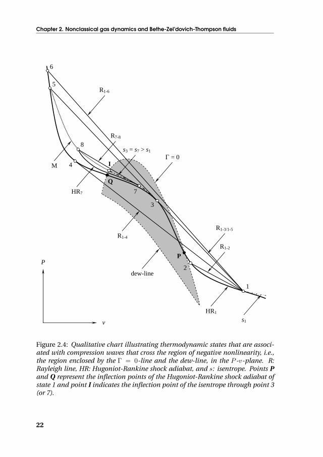
The thermodynamic property Γ is referred to as the fundamental derivative ofgas dynamics due to its importance in many facets of compressible gas dynam-ics [196, 41, 42, 46, 47]. These include not only shock-wave theory, but also thestudy of isentropic and Fanno flows of dense gases. Formulated in terms of thefundamental derivative of gas dynamics, a polytropic ideal gas can only admitcompression shock waves and expansion fans, whilst satisfying the thermody-namic and mechanical constraints (as is to be demonstrated in Sec. 2.1), exclu-sively because Γ = (γ + 1) /2 > 1 > 0, where γ is the ratio of the isobaric heatcapacity with respect to the isochoric heat capacity, i.e., γ ≡ CP /Cv. If real-gaseffects are taken into account and if Γ changes sign and becomes negative, seeFig. 1.1, the resulting finite interval of concavity of the strictly monotonous P -v-isentropes enables the admissibility of expansion shock waves, compressionfans, and composite waves, whilst satisfying the thermodynamic and mechani-cal constraints (see Sec. 2.1). The composite wave fields are the result of mixednonlinearity, that is, they result from the fact that Γ, at least locally, changes itssign.
That Γ can indeed be negative can be explained by considering the behav-ior of the critical isotherm in the P -v-plane. It is known that at the criticalpoint both (∂P/∂v)T and
(∂2P/∂v2
)T
of the critical isotherm are zero and that
2

1.2 Motivation and thesis outline
in the ideal-gas limit, the critical isotherm is convex. Moreover, the isother-mal compressibility, κT ≡ −1/v (∂v/∂P )T , is positive for all substances in allphases. The critical isotherm therefore, must display a limited interval of con-cavity located between the critical specific volume vC and the ideal-gas limitwhere v → ∞. For substances composed of sufficiently complex polyatomicmolecules, as classified in Ref. [29], due to the large isochoric heat capacity(excluding the critical region), the behavior of isentropes is similar to that ofisotherms and for this reason, isentropes also feature a region of concavity. In-deed, both Bethe [14] and Zel’dovich [231] have independently shown that Γ canbecome negative for a polytropic Van der Waals fluid provided that the ideal-gasisochoric heat capacity is sufficiently large.1 Figure 1.1 shows the region of Γ < 0for a hypothetical polytropic Van der Waals fluid with large ideal-gas isochoricheat capacity; examples of real fluids that exhibit a region of Γ < 0 are providedin Sec. 4.1.
Apart from the analysis of nonclassical phenomena admissible in the single-phase dense-gas region, Zel’dovich and Raizer [232] have pointed out that ex-pansion shock waves can also occur during polymorphic phase transition insolids due to the discontinuity of isentropes such that Γ → −∞ at the phaseboundary. See the paper by Ivanov and Novikov [103] on the observation of ex-pansion shock waves in iron due to solid-solid phase transition and Ref. [11] onexpansion shock waves observed in fused silica which is an amorphous solid.Similarly, Γ → −∞ for certain thermodynamic states located on the vapor-and liquid saturation lines of a retrograde fluid, as first demonstrated by Bethe,ergo supersonic flows of retrograde fluids with phase changes also exhibit phe-nomena associated with mixed nonlinearity, e.g., evaporation expansion shockwaves (refer for example to the works of Thompson and coworkers, e.g., Refs.[202, 199, 200]). Because of the pioneering work of Bethe, Zel’dovich and Thomp-son in the field of nonclassical gas dynamics, i.e., the study of compressiblewave fields in the dense-gas thermodynamic regime of a molecularly complexcompound, substances that exhibit a region of Γ < 0 in the single-phase dense-gas regime are known as Bethe-Zel’dovich-Thompson (BZT) fluids [45], and phe-nomena that ensue from the fact that a substance has an embedded region ofnegative nonlinearity (region of Γ < 0) are referred to as BZT effects.
1.2 Motivation and thesis outline
In spite of the important amount of theoretical knowledge gained especially inthe last 35 years, no successful experimental observation of BZT effects in a gasis available. To the knowledge of the author, two attempts to demonstrate BZTeffects in single-phase dense-gases have been made in the past. The first of
1According to Ref. [201], Bethe however dismissed the fact that real fluids can display a region offinite size where Γ < 0.
3

Chapter 1. Introduction
these is the experiment reported by Borisov et. al. [17, 119]. However, the resultreported in Ref. [17] on the observation of a single-phase expansion shock wavehas been criticized by Fergason [65] as not providing experimental evidenceof a single-phase expansion shock wave. Fergason’s assessment was based onthe fact that model EoS’s (as are the cubic EoS’s) and multiparameter EoS’s donot predict freon-13, i.e., the test fluid used by Borisov et. al., to exhibit a re-gion of Γ < 0 in the dense-gas thermodynamic regime. Moreover, Fergasondemonstrates numerically that the expansion wave created and documentedin Ref. [17] potentially displays phase transition and/or non-equilibrium tran-sition. The second experiment is the one conducted by Fergason and docu-mented in his PhD thesis [65]; Fergason’s experiment was not successful due tothermochemical decomposition of the test fluid, namely a perfluorocarbon, at
v/vC [-]
P/P
C[-
]
0.5 1.0 1.5 2.0 2.5 3.00.6
0.7
0.8
0.9
1.0
1.1
Convex
Convex
Concave
Γ = 0
Figure 1.1: The shaded area represents the region where Γ < 0 for a hypotheticalpolytropic Van der Waals fluid with Cv/R = 50 (Cv is the specific isochoric heatcapacity and R is the specific gas constant). Also shown are an isentrope whichexhibits both convex and concave behavior (solid line) and an isotherm (dashedline). ◦: thermodynamic states where the isentrope has its inflection points, vC
denotes the critical specific volume and PC is the critical pressure.
4

1.2 Motivation and thesis outline
the high experimental temperature.Experimental evidence of nonclassical gas-dynamic effects in general is im-
portant for further progress in the field of compressible fluid dynamics. The mo-tivation of this research stems from the need of such an experiment to demon-strate the existence of nonclassical gas-dynamic phenomena in dense gases ofmolecularly complex fluids, the most intriguing of which is the theoretical ad-missibility of expansion shock waves. Furthermore, nonclassical gas-dynamicphenomena can be exploited in technical applications operating in the dense-gas regime or in transonic or supersonic conditions. One such example is theutilization of BZT effects in organic-Rankine-cycle engines, where, under suit-ably chosen conditions, shock wave formation can be avoided or, as far as shockwaves are generated, they are weak and boundary layer detachment is sup-pressed. This behavior which is typical of BZT fluids, can be beneficial duringpart-load operation of the organic-Rankine-cycle engine.
The aim of this research is to develop, design, build and commission an ex-perimental facility which can be used to generate and study nonclassical ex-pansion shock waves in molecularly complex substances classifying as poten-tial BZT candidates. Secondarily, the facility that is to be built must be modularand flexible in its design and should therefore allow for investigating both classi-cal and nonclassical dense-gas flows. Moreover, cascading from the main goal,relevant theory has been developed. The results of these investigations are alsouseful/necessary for validating the proprietary software package zFlow [36], i.e.,a CFD software package for compressible gas-dynamic simulations using real-gas properties [38].
The thesis is structured as follows. Firstly, Chap. 2 outlines the theoreticalbackground with respect to shock waves, where, starting from the formation ofshock waves in general, the admissibility of unconventional gas-dynamic dis-continuities like the mentioned expansion shock waves, is treated. The thermo-dynamic description of the fluid is key to both identifying potential BZT candi-dates, and to the design of an experimental facility in which nonclassical wavefields are to be formed. Herein, prior to the development of a thermodynamicmodel of the fluid, the use of the EoS for the design and analysis of technical ap-plications was also taken into consideration. For this purpose, Chap. 3 treats thedevelopment of consistent multiparameter EoS’s for dimethylsiloxanes, whichin this study have been selected as test fluids. Dimethylsiloxanes have been cho-sen for the envisaged experiment(s) because of their favorable characteristicsregarding the design of the facility, e.g., limited flammability and toxicity, andfrom the viewpoint of the application of the results of this research in the nearfuture, e.g., the development and testing of organic-Rankine-cycle turbines. Ac-curate computation of the value of the fundamental derivative of gas dynamicsis a necessity for understanding and describing real-gas processes occurring inthe dense-gas regime. The influence of the functional relation of the thermody-namic model regarding the computation of Γ is discussed in Chap. 4. This in-cludes a study of Γ in the single- and two-phase critical region using physically
5

Chapter 1. Introduction
based scaling laws. After these preliminary chapters which are mainly relatedto theory, Chap. 5 discusses experimental options that can be used to generatean expansion shock wave in a BZT fluid. The assessment of a variety of pos-sible and technically feasible experimental options has resulted in the choiceof an experiment and thus of a facility which incorporates the operational ease,modularity and versatility of both the variable-cross-section shock tube and theLudwieg tube. The preliminary design of this facility is treated in Chap. 6 andthe commissioning of the setup as built, is discussed in Chap. 7. Finally, Chap. 8summarizes conclusions and recommendations for future research activities.
Nomenclature
Symbol Description
CP Specific isobaric heat capacityCv Specific isochoric heat capacityc Thermodynamic speed of soundP PressureR Specific gas constants Specific entropyT Absolute temperaturev Specific volume
Γ Fundamental derivative of gas dynamicsγ Heat capacity ratioκT Isothermal compressibilityρ Density
6

“Do you have blacks, too?”
President George W. Bush speaking to President FernandoCardoso, Washington, D.C., November 8, 2001
2Nonclassical gas dynamics and
Bethe-Zel’dovich-Thompson fluids
Abstract
Dense gases of so-called Bethe-Zel’dovich-Thompson (BZT) fluids can theoret-ically display unusual gas-dynamic phenomena, notably the admissibility ofsingle-phase expansion shock waves and compression fans. That these phe-nomena – which are typical only of BZT fluids if the pressure and temperatureare of the order of their vapor-liquid-critical-point value – are considered un-conventional, stems from the fact that experimental evidence is unavailable.It is the goal of this chapter to present the theoretical background of the fieldof science, nowadays referred to as nonclassical gas dynamics. More specifi-cally, the focus herein is on how a compound is classified as being a BZT fluidand what the conditions are that give rise to the admissibility of nonclassicalgas-dynamic phenomena. The contents of this chapter are as follows: for thesake of completeness, Sec. 2.1 provides a brief introduction to the theory ofshock waves, treating the formation of shock waves, the shock admissibilityconditions, and the structure of weak shock waves. The subsequent sections,Secs. 2.2 and 2.3, respectively give a qualitative description of compression andexpansion waves traversing the negative-nonlinearity region, i.e., the Γ < 0-region. Furthermore, double sonic shock waves, these are the strongest expan-sion shock waves that can be admitted, and maximum-Mach expansion shockwaves, these are shock waves with the greatest supersonic to sonic transition,are discussed. These nonclassical BZT effects are important also from an exper-
7

Chapter 2. Nonclassical gas dynamics and Bethe-Zel’dovich-Thompson fluids
imental viewpoint.
2.1 Theory of shock waves in the dense-gas regime
A shock wave is defined as a relatively thin geometric surface through whichthere is flow of matter which experiences abrupt, seemingly discontinuous, vari-ation of state. This type of mechanical wave originates when a substance is sub-jected to rapid compression or expansion. The evolution of an initially smoothdisturbance into a discontinuity was theoretically discovered by Riemann [170],Rankine [167] and Hugoniot [97]. Following the mathematical treatment of Rie-mann, consider a (quasi-) one-dimensional flow through a duct of constantcross-sectional area with an initially continuous density and velocity profile. Ifin addition the flow is homentropic, i.e., Ds/Dt = 0 ∧ ∇s = 0, where D/Dt rep-resents the material (convective) derivative and ∇ denotes the gradient vector,and if body forces can be neglected, the conservation equations for mass andmomentum are of the form (if required, refer to the list at the end of this chap-ter explaining the adopted nomenclature)
∂ρ
∂t+ ρ
∂u
∂x+ u
∂ρ
∂x= 0
∂u
∂t+ u
∂u
∂x+
1ρ
∂P
∂x= 0.
(2.1)
Here, P is the pressure, t is the time, u is the absolute velocity, x represents thespatial coordinate, and ρ denotes the fluid density. Because the flow is homen-tropic, the pressure is related to the density as1
∂P
∂x= c2
∂ρ
∂x, (2.2)
where c is the thermodynamic speed of sound. Substitution of Eq. (2.2) in theconservation equations yields
∂ ln ρ∂t
+∂u
∂x+ u
∂ ln ρ∂x
= 0
∂u
∂t+ u
∂u
∂x+ c2
∂ ln ρ∂x
= 0.
(2.3)
Next, identify the thermodynamic function
F (ρ (x, t)) ≡ρ∫
ρ0
cd (ln ρ) =
P∫P0
dP
ρc=
c∫c0
dc
Γ− 1, (2.4)
1For isentropic flows, Eq. (2.2) is valid along individual streamlines.
8

2.1 Theory of shock waves in the dense-gas regime
whereby the subscript “0” in the lower limit of integration represents a referencestate and Γ is the fundamental derivative of gas dynamics defined in Eq. (1.1) inChap. 1. The function F (x, t) is meaningful only for isentropic flows, i.e., flowsthat satisfy Ds/Dt = 0. Furthermore, for reasons that will become clear in thefollowing, introduce the notation J + (x, t) ≡ u (x, t) + F (x, t) and J− (x, t) ≡u (x, t) − F (x, t). Formulated in terms of F (x, t) and J± (x, t) and after somesymbolic manipulation, the governing equations of the flow reduce to
(∂
∂t+ (u− c) ∂
∂x
)J− = 0
(∂
∂t+ (u+ c)
∂
∂x
)J + = 0.
(2.5)
The governing equations of the flow, as formulated in Eqns. (2.5), are first-orderquasi-linear hyperbolic partial differential equations of the form
α1 (x, t)︸ ︷︷ ︸= 1
∂J±
∂t+ α2 (x, t)︸ ︷︷ ︸
= u±c
∂J±
∂x+ α3 (x, t)︸ ︷︷ ︸
= 0
J± = 0, (2.6)
provided that J± 6= 0. First-order quasi-linear hyperbolic partial differentialequations can be solved using the method of characteristics whereby the initialproblem which is formulated in terms of (x, t), is converted into a new coor-dinate system (x0, l) in which each partial differential equation is transformedinto two ordinary differential equations along certain curves, namely character-istic curves described by {[x (l) , t (l)] : 0 < l <∞}, in the x-t-plane. Variable x0
changes only along the initial curve in the x-t-plane, so at t = 0, and it remainsconstant along the characteristic curve; conversely, variable l changes alongthe characteristic curve. The characteristic curves for Eqns. (2.5) are dt/dl =α1 (x, t) = 1 and dx±/dl = α2 (x, t) = u ± c, where α2 (x, t) represents the wavespeed (or convected sound speed). It equals u + c for positive waves or so-called right-running characteristics and u−c for negative wave or so-called left-
running characteristics.2 Then dJ±/dl = ∂J±/∂t + (u± c) ∂J±/∂xEqns. (2.5)
= 0,implying that J± are invariant along their respective characteristic curves, tak-ing the aforementioned assumptions into consideration. In general, each char-acteristic curve i has a different J±i which remains constant along the curve.The method just described, if applied to Eqns. (2.5), allows for the determina-tion of weak solutions – these are solutions that may have a discontinuity, maynot be differentiable everywhere and that may be less smooth – like for exampleshock waves.
2This definition of positive and negative waves is based on the standard that in one dimension,rightward pointing vectors are positive and leftward pointing vectors are negative.
9

Chapter 2. Nonclassical gas dynamics and Bethe-Zel’dovich-Thompson fluids
To illustrate the coalescence of an initially continuous wave into a shockwave, consider a weak triangular pressure disturbance shown in Fig. 2.1 prop-agating into the positive x-direction (so towards to right). Such a wave can becreated by moving a piston forward and backward. In this context “weak” im-plies that Pmax/P0, with P0 the pressure at the undisturbed state, is of the orderunity such that irreversible effects can be neglected. Using the results of theprevious paragraph for simple waves, it is found that (see also Ref. [197])
dσ+ = d (u+ c) =ΓρcdP, (2.7)
P
x
t
P
x
t
Figure 2.1: Above: the σ+i -convected-sound-waves (dashed lines) converge for the
compressive part of the pressure disturbance to form a compression shock wave.The (shock) wave classifies as simple and moves into a region of uniform flow.The wave distortion is the result of an increase of the wave-speed u + c at higherpressure with respect to P0, because Γ > 0 and does not change sign across thewave. The σ−i -convected-sound-waves are not shown.Below: the σ+
i -convected-sound-waves (dashed lines) converge for the expansivepart of the pressure disturbance to form an expansion shock wave. The (shock)wave classifies as simple and moves into a region of uniform flow. The wave dis-tortion is the result of a decrease of the wave-speed at higher pressure with respectto P0, since Γ < 0 and does not change sign across the wave. The σ−i -convected-sound-waves are not shown.
10

2.1 Theory of shock waves in the dense-gas regime
wAt ~ єz
wAn
n t
p
nB
nA
uB
uA
b
shock wave ~z
wA = uA-b
wB = uB-b wBn
wBt
shock wave
Figure 2.2: The shock front locally enclosed by an arbitrarily thin control volume.Left: velocities according to an observer moving with the shock wave. Right: ve-locities according to a laboratory frame of reference. The indices A and B refer tothe pre- and post-shock state respectively, and u = absolute velocity (u = ‖u‖),w = relative velocity (w = ‖w‖), b = shock speed (b = ‖b‖), and n = unit vec-tor locally normal to the surface parallel to the shock wave (by definition positiveif outward-pointing). The unit vectors (n, t,p) form an orthogonal set (basis).Furthermore, z denotes a representative length and ε is an arbitrarily small num-ber, such that if z → 0, volume integrals in the conservation equations can beneglected.
meaning that if Γ > 0 it is implied that the wave speed increases with an increasein pressure and therefore an initially continuous compressive wave eventuallycoalesces into a compression shock wave, i.e., a shock wave whereby the pres-sure increases in the direction of the flow as seen by an observer moving withthe discontinuity. On the other hand, if Γ < 0 it is implied that the wave speeddecreases with an increase in pressure and therefore an initially continuous ex-pansive wave eventually coalesces into an expansion shock wave, i.e., a shockwave whereby the pressure decreases in the direction of the flow as perceivedby an observer moving with the discontinuity.
Note that the analytical treatment of Riemann on shock-wave formation asjust described, is only valid for weak shock waves and it is based on the im-plicit assumption that the shock wave is without structure. Furthermore, theRiemann description of shock-wave formation fails as soon as characteristicsintersect, since this implies multivaluedness of properties. There exists no gen-eral solution at present that describes all successive stages during the formationof strong shock waves, whereby, for example, it may be necessary to account forrelaxation effects in polyatomic vapors preceding the appearance of the geo-metric surface of discontinuity.
11

Chapter 2. Nonclassical gas dynamics and Bethe-Zel’dovich-Thompson fluids
From the instant of shock-wave formation and onwards, the flow is no longerhomentropic and further description of the flow field, if one is not interestedin the structure of the shock wave, requires the use of the Hugoniot-Rankinejump conditions. The development of these relations between pre- and post-shock states A and B respectively, is based on the laws of conservation of mass,momentum and energy applied to a control volume which locally encloses theshock front and which moves with the shock velocity b, see Fig. 2.2. The pre-shock state is indicated by A and the post-shock state by B. Under the suppo-sition that the shock wave represents a discontinuity separating two regions ofthermodynamic-equilibrium states, the control volume can be made arbitrar-ily thin. Furthermore, the area of the edges of the control volume which areperpendicular to the shock front, are negligible with respect to the surface-areaparallel to the shock front. Applying the laws of conservation of mass, momen-tum and energy to the control volume, as seen by an observer moving with theshock wave, yields per unit area of shock-front-surface
−ρAwAn + ρBwBn = 0 (2.8)
−ρAuAwAn + ρBuBwBn = −PBnB − PAnA (2.9)
−ρA
(eA +
u2A
2
)wAn +ρB
(eB +
u2B
2
)wBn = −PBnB ·uB−PAnA ·uA, (2.10)
where wAn ≡ − (uA−b) · nA and wBn ≡ (uB−b) · nB are the magnitudes of therelative velocities of the fluid normal to the shock-front surface in the pre- andpost-shock states respectively, (PA, ρA) and (PB, ρB) are the pressure and den-sity of the pre- and post shock states respectively, and eA,B denotes the specificinternal energy of the substance in the pre-, respectively post-shock state.
Following Thompson [198], the momentum and energy conservation equa-tions can be simplified. With nA = −nB and by adding to the momentum equa-tion, which is a vector equation, b (ρAwAn − ρBwBn) = 0, Eq. (2.9) reduces to
−ρA (uA−b)wAn + ρB (uB−b)wBn = nA (PB − PA) . (2.11)
Taking the dot product of the momentum equation and the orthogonal set ofunit vectors (n, t,p), see Fig. 2.2, yields respectively
PA + ρAw2An = PB + ρBw
2Bn (2.12a)
wAt = wBt (2.12b)
wBp = 0. (2.12c)
12

2.1 Theory of shock waves in the dense-gas regime
Equation (2.12c) implies that the flow velocity in the post-shock state is in theplane of vectors n and t and Eq. (2.12b) states that locally, the component ofthe relative velocity which is parallel to the shock front is invariant. CombiningEq. (2.12a) with the continuity equation and multiplying both the left- and right-hand-side of the relation by ρAρB gives
J2 ≡ (ρAwAn)2 = (ρBwBn)2 = −PB − PA
vB − vA, (2.13)
with J the mass flux. This equation represents a straight line in the P -v-planeconnecting the pre- and post-shock states with a slope of −J2 and it is referredto as the Rayleigh line.
The energy conservation equation can be simplified by addition of the term(PBwBn − PAwAn) to both the left- and right-hand-side of Eq. (2.10) and by em-ploying the continuity and momentum equations and the definition equationfor enthalpy h ≡ e+ P/ρ, yielding
hB +u2
B
2−(hA +
u2A
2
)= b · (uA−uB) . (2.14)
Since ‖u− b‖2 = w2n +w2
t and according to Eq. (2.12b)wt is invariant across theshock front, the energy balance equation simplifies to
hA +w2
An
2= hB +
w2Bn
2. (2.15)
Further symbolic manipulation finally results in
hB − hA =12
(PB − PA) (vB + vA) . (2.16)
This equation, obtained independently by Rankine [167] and Hugoniot [97],is rather convenient since it contains only thermodynamic properties and itis independent of the reference frame. This so-called Hugoniot-Rankine (HR)shock adiabat applies to general shock discontinuities, and, for a given pre-shock state, say A, a locus of possible post-shock thermodynamic states can bedrawn, say for example in a P -v-diagram.
As a consequence of the abrupt changes of properties across the shock wavewhich bring about large temperature and velocity gradients, the transformationfrom state A to state B across the shock wave occurs irreversibly. The gradi-ent in temperature for example results in irreversible heat flow and the gradi-ent in velocity enhances viscous dissipation in the shock wave.3 Additionally,relaxation of the vibrational degrees of freedom can become important, espe-cially for polyatomic fluids, either immediately upstream or downstream of the
3Note that Riemann incorrectly assumed the flow to be isentropic even after shock wave forma-tion.
13

Chapter 2. Nonclassical gas dynamics and Bethe-Zel’dovich-Thompson fluids
shock wave. Ergo, apart from the principal shock conditions which stem fromthe conservation laws, the entropy must increase across a shock wave. More-over, according to Lax [124] and Oleinik [158] a fifth condition (referred to asthe (mechanical) stability criterium or speed-ordering condition) is required foradmissible shock waves, namely that the pre-shock Mach number – defined asMaAn ≡ wAn/cA – must be greater than or at least equal to unity and that thepost-shock Mach number, i.e., MaBn ≡ wBn/cB, must be less than or at leastequal to unity.4 In summary, admissible shock waves must satisfy all of the fol-lowing shock conditions:
[ρwn] = 0 (2.17a)[P + J2v
]= 0 (2.17b)[
h− (vA + vB)2
P
]= 0 (2.17c)
[s] ≥ 0 (2.17d)
MaAn ≥ 1 ≥ MaBn, (2.17e)
whereby the square brackets represent the jump of a quantity across the shockwave, e.g., [Υ] = ΥB −ΥA.
As was already mentioned, both the entropy condition and the stability cri-terium, unlike the conservation laws, impose a direction on the transformationthat can occur in shock waves. By means of the purely mathematical treatmentof Riemann, it was demonstrated that compression shock waves form if Γ > 0and that expansion shock waves form if Γ < 0. Moreover, the treatment of Rie-mann starts with an initially continuous disturbance which evolves in time intoa discontinuity. Alternatively, it is also possible to distinguish admissible solu-tions from inadmissible solutions by performing a Taylor-series expansion ofthe HR shock adiabat with h (s, P ), which represents a fundamental EoS (seeDuhem [57], Becker [12], and Bethe [14], and Courant and Friedrichs [39]). Forweak shock waves the result is
∆s =
=0︷ ︸︸ ︷(∂s
∂P
)HRA,A
× (P − PA) +12!
=0︷ ︸︸ ︷(∂2s
∂P 2
)HRA,A
× (P − PA)2
+13!
(∂3s
∂P 3
)HRA,A
× (P − PA)3 +O[(P − PA)4
]⇒
[s] = (sB − sA) ≈ ΓAP3A
6TAρ3Ac
4A
[PB/PA − 1]3 ≥ 0. (2.18)
Here, it has implicitly been assumed that Γ, defined in Eq. (1.1), does not changeits sign as a result of the pressure disturbance due to the wave and that it is
4For strictly convex or hypothetically strictly concave isentropes, the entropy condition and thestability criterium are equivalent [114].
14

2.1 Theory of shock waves in the dense-gas regime
not equal to zero, and that there is thermodynamic equilibrium. In Eq. (2.18),(∂ js/∂P j
)HRA,A
is the short notation for the j-th order derivative (j = 1 . . . 3)
of entropy with respect to pressure along the HR shock adiabat of pre-shockstate A, evaluated at state A. It is readily demonstrated that weak compressionshock waves, these are shock waves with PB/PA & 1, are admissible if Γ > 0and that weak expansion shock waves, namely shock waves with PB/PA . 1,are admissible if Γ < 0.5 An in-depth analysis about the entropy jump acrossa shock wave featuring a change of sign of Γ as a result of the pressure waveis conducted by Cramer and Kluwick [48]. Additional results from the Taylor-series expansion are that at a pre-shock state A, the HR shock adiabat of stateA and the isentrope through point A have the same slope and curvature in theP -v-plane; formally,
(∂P
∂v
)HRA,A
=(∂P
∂v
)s,A(
∂2P
∂v2
)HRA,A
=(∂2P
∂v2
)s,A
.(2.19)
Hitherto, the structure of the shock waves has not been considered. This isnot surprising since negligence of thermoviscous effects in the governing equa-tions only allows for the admissibility of discontinuous solutions from a math-ematical point of view. Consequently, dissipative effects are assumed to oc-cur only in the discontinuity. The processes of dissipation represent a complexsequence of non-equilibrium transition from one thermodynamic equilibriumstate to another thermodynamic equilibrium state, whereby the time which isrequired for completing the transition, determines the thickness of the shockwave [193]. Thermodynamic equilibrium implies the equilibrium distributionof energy over all molecular, atomic and electronic degrees of freedom. Thestructure of the shock wave is governed by the rate and type of relaxation pro-cess that occurs in it. The relaxation process is defined as that of establishingthermodynamic equilibrium and it is, for example, a result of a delay in energytransfer between various internal degrees of freedom. In the case of weak shockwaves where the gradients of flow variables are sufficiently small, the structureof the wave can completely be described by the Navier-Stokes equations for aviscous and conducting fluid. In the case of strong shock waves the situation isvery different. Strong shock waves contain a thin leading layer through whichflow variables change quite abruptly. The thickness of this so-called shock frontis of the order of the mean-free-path for translational relaxation, consequently,from a macroscopic viewpoint, this leading transitional layer is a gas-dynamic
5This procedure does not treat weak pressure disturbances that traverse the negative nonlin-earity region, see Fig. 1.1; it is only intended as a demonstration that expansion shock waves aretheoretically possible without violation of the second law of thermodynamics. Locally, the stabilitycriterium is also satisfied because of local convexity or concavity of the strictly monotonous isen-tropes, depending on the sign of ΓA.
15

Chapter 2. Nonclassical gas dynamics and Bethe-Zel’dovich-Thompson fluids
discontinuity and at the discontinuity, the fluid is not a continuum. This resultsin a significant departure of thermodynamic equilibrium of the vapor imme-diately behind the shock front. A qualitative illustration of the relaxation zonebehind a shock front is presented in Fig. 2.3. Thermodynamic equilibrium isattained through, as was previously mentioned, a succession of complex relax-ation processes via excitation of rotational, vibrational and electronic degreesof freedom, each of which can be characterized by a relaxation time τ . Gen-erally, τtrans < τrot � τvib, i.e., the vibrational relaxation is much slower withrespect to rotational relaxation and translational relaxation, or alternatively, themean-free-path for vibrational relaxation is significantly greater than that forrotational relaxation and translational relaxation, respectively. This is the resultof the low efficiency of energy transfer between vibrational and translational de-grees of freedom on molecular collisions. Moreover, the majority of polyatomicmolecules display a single relaxation process whereby the whole of the vibra-tional energy relaxes via the lowest mode, see Ref. [120] and Chap. 3, pg 64 ofRef. [121]. In this situation, the vibrational relaxation time is estimated fromthe Lambert-Salter plot [121] and the shock wave thickness can be estimated.Yet, exceptions have been found where nonlinear (vibrational) relaxation oc-curs, see for example Kiefer et. al. [108]. Under these circumstances it is thendifficult or even impossible to estimate the shock wave thickness or to assesswhether the hypothesis of thermodynamic equilibrium is valid.
Since the shock waves that are of interest herein are weak, the thickness canbe determined by taking into account the dissipative processes under the pro-vision that the continuum hypothesis is still valid. For this purpose, the secondlaw of thermodynamics is employed. As derived by Thompson [198] (see alsoBorisov [17]), the entropy balance statement equals
ρDsDt
=ΦT
+1T∇ · (κ∇T ) , (2.20)
where κ is the thermal conductivity and the scalar Φ is the dissipation functiondefined as
Φ =23η[(D11 −D22)2 + (D22 −D33)2 + (D33 −D11)2
](2.21)
+ 4η(D2
12 +D213 +D2
23
)+ ζ (D11 +D22 +D33)2
.
In Eq. (2.21), η is the dynamic viscosity, ζ is the bulk (volume) viscosity,6 andDik = Dki is the so-called rate-of-deformation tensor defined as
Dik ≡12
(∂wi∂xk
+∂wk∂xi
). (2.22)
6ζ = λ+2
3η, where λ is the second viscosity coefficient.
16

2.1 Theory of shock waves in the dense-gas regime
Relaxation zone: establishment of statistical equilibrium
Shoc
k w
ave
fron
t
Elastic collisions as in monatomic gases. Maxwellian distribution for translational velocity is established. This is not the case for the energy distribution with respect to other degrees of freedom (retarded energy transfer)
wA wB
States A and B are related via the HR-shock relations whereby it is assumed that the thermodynamic variables are equal to their values in the state of complete thermodynamic equilibrium.
Shock wave thickness (an arbitrary definition)
Figure 2.3: Illustration of the relaxation zone behind a shock wave in a poly-atomic gas. In the shock wave front equilibrium between the translational androtational degrees of freedom is established (assuming that the time required fortranslational and rotational relaxation are of the same order of magnitude, thelatter being greater), whereas the establishment of equilibrium over the vibra-tional degrees of freedom occurs behind the front.
Noting that
1T∇ · (κ∇T ) = ∇ · κ∇T
T︸ ︷︷ ︸`
+κ
T 2(∇T )2 (2.23)
and assuming i) one-dimensional flow (or nearly so), ii) stationary conditions,
17

Chapter 2. Nonclassical gas dynamics and Bethe-Zel’dovich-Thompson fluids
iii) fixed-valued transport properties, and accounting for the kinetic energy term,gives for Eq. (2.20),
Tρw
(ds
dx
)=(
43η + ζ
)(dw
dx
)2
+d
dx
(κdT
dx
). (2.24)
If dT/dx ≈ [T ] /ε, ds/dx ≈ [s] /ε, and dw/dx ≈ [w] /ε, where ε is the shock thick-ness, and considering that (refer to Eq. (2.18))
[s] = ΓA [P ]3 /(6TAρ
3Ac
4A
), (2.25)
and that vector ` in Eq. (2.23) vanishes at the boundaries, then the shock wavethickness can be approximated by
ε =
[(43η + ζ
)[w]2 +
κ [T ]2
TA
]6ρ2
Ac3A
MaAΓA [P ]3. (2.26)
States A and B are chosen sufficiently far from the shock wave. It is seen thatfor a nonconducting, inviscid fluid, the shock wave thickness is equal to zero, asis to be expected. Also, if the shock wave is very weak such that PB is less thanbut approximately equal to PA, i.e., a rarefaction shock wave, or if ΓA is veryclose to zero (and negative), ε becomes very large. The last example indicatesthe arbitrariness of this “definition” of shock wave thickness. Thompson andLambrakis [201] for example use the criterium of 98.7 % of the overall speedchange across the shock wave to determine its thickness. From this criteriumand assuming that the bulk viscosity is of the same order of magnitude as thedynamic viscosity, Thompson and Lambrakis estimate the thickness of expan-sion shock waves to be of the order of 1 µm. This approximate value for theshock wave thickness is sufficiently large and thus the continuum hypothesis isindeed valid.
2.2 Compression waves through the BZT-region
The determination of admissible solutions of the governing equations for shockwaves, see Eqns. (2.17), is usually conducted graphically. As was demonstratedin Sec. 2.1, Eq. (2.13) for example represents a straight line in a P -v-diagramconnecting the pre-shock state with possible post-shock solutions. Similarly,the HR shock adiabat represented by Eq. (2.16) is invariant of the frame of ref-erence and by approximation, it represents mathematical solutions of the en-ergy conservation equation across a shock wave. Since the intersection of theHR shock adiabat and the Rayleigh line implies that there is conservation ofmass, momentum and energy, the second law of thermodynamics and the sta-bility criterium are used to distinguish between admissible solutions and math-ematical solutions that are physically not allowed (inadmissible). Anticipating
18

2.2 Compression waves through the BZT-region
the results outlined in detail by Kluwick [114] and summarized in the para-graphs hereinafter, an in-depth analysis of the relations developed in Sec. 2.1has revealed that admissible solutions of the governing equations can be distin-guished from inadmissible ones by employing geometrical arguments and byusing visual information in a P -v-diagram.
First, consider the HR shock adiabat of a pre-shock state denoted by A. Be-cause of the fact that at the pre-shock state the HR shock adiabat of state Aand the isentrope through point A have the same slope (and curvature), seeEq. (2.19),
(∂P
∂v
)HRA,A
= − c2A
v2A
. (2.27)
Here, (∂P/∂v)HRA,Ais the short notation for the slope of the HR shock adiabat of
state A, evaluated at state A. The equation for the Rayleigh line in combinationwith Eq. (2.27) gives for the pre-shock stability criterium MaA ≥ 1 that
(∂P
∂v
)HRA,A
≥ [P ][v]
. (2.28)
Thus, for admissible shock waves A–B, the absolute value of the slope of the HRshock adiabat of state A, evaluated at state A, is less than or at most equal to theabsolute value of the slope of the Rayleigh line connecting states A and B.
Next, the graphical interpretation of the MaB ≤ 1-shock-admissibility cri-terium is illustrated. For this purpose consider the HR shock adiabat throughpre-shock state A, and passing through a possible post-shock solution B. Appli-cation of the thermodynamic identity Tds = dh − vdP (Tds-equation) to post-shock state B gives
TBdsB = dhB − vBdPB =︸︷︷︸HRA,B
(vA + vB
2dPB +
PB − PA
2dvB
)− vBdPB
= − [v]2dPB +
[P ]2dvB, (2.29)
where HRA,B is the short notation for the HR shock adiabat of state A, evaluatedat state B. Furthermore, at state B, the variation of pressure can be expressed
19

Chapter 2. Nonclassical gas dynamics and Bethe-Zel’dovich-Thompson fluids
according to
dPB =(∂P
∂s
)v
(sB, vB) dsB +(∂P
∂v
)s
(sB, vB) dvB
= TB
(∂P
∂e
)v
(sB, vB) dsB −c2Bv2
B
dvB ⇒
TBdsB =dPB +
c2Bv2
B
dvB(∂P
∂e
)v
(sB, vB)
=dPB +
c2Bv2
B
dvB
GB/vB
, (2.30)
with GB ≡(βP c
2/γCv)
Band βP ≡ (∂ ln v/∂T )P > 0 is the coefficient of volume
expansion.7 Equating the right-hand-sides of Eqns. (2.29) and (2.30) yields(∂P
∂v
)HRA,B
− [P ][v]
=c2Bv2
B
(Ma2
B − 1)(
1 +[v]2vB
GB
) . (2.31)
The stability criterium applied to the post-shock state then gives(∂P
∂v
)HRA,B
≤ [P ][v]
, (2.32)
under the provision that: i) 1 + [v]GB/ (2vB) 6= 0, ii) βP > 0, and iii) that thesolution, viz. post-shock state B, in a P -v-plane is located to the right of thesingularity.
Thus, for admissible shock waves A–B, it follows from condition (2.32) that theabsolute value of the slope of the HR shock adiabat of state A, evaluated at stateB, is greater than or at least equal to the absolute value of the slope of the Rayleighline connecting states A and B.
Because in the limit of down-stream sonic shock waves
[P ][v]
=(∂P
∂v
)HRA,B
, (2.33)
7Cases where βP ≤ 0 are excluded.
20

2.2 Compression waves through the BZT-region
it can be inferred from Eq. (2.29) that at sonic point B on the shock adiabat ofpoint A,(
∂s
∂v
)HRA,B
= 0. (2.34)
If the Tds-equation is applied across the shock wave
stateB∫stateA
Tds =
stateB∫stateA
de+
stateB∫stateA
Pdv = ∆e+
stateB∫stateA
Pdv
= −PA + PB
2[v] +
stateB∫stateA
Pdv = AHRA −ARA−B ≥ 0, (2.35)
with A representing the area between vA and vB under either the HR shock adi-abat or the Rayleigh line, depending on de subscript.
This result together with Eq. (2.34) indicate that for admissible downstream sonicshock waves, the sonic point has a local extremum in entropy.
In summary:
- According to the stability criterium, all admissible shock waves satisfy(∂P
∂v
)HRA,B
≤ [P ][v]≤(∂P
∂v
)HRA,A
; (2.36)
- An admissible downstream sonic post-shock state is a local maximum [114]in entropy;
- From Eqns. (2.17d), (2.35) and (2.36) it follows that the Rayleigh line mustnot intersect the HR shock adiabat at an interior point and therefore, theRayleigh line connecting the pre- and post shock states must be locatedeither completely above the HR shock adiabat (this means that compres-sion shock waves are admissible) or completely below the HR shock adia-bat (this means that expansion shock waves are admissible) [114, 124, 41].
To elucidate the use of the geometrical arguments, consider compressivewaves originating from an upstream thermodynamic state 1 located in the dense-gas thermodynamic regime to the right of the region of negative nonlinearity,see Fig. 2.4, such that the isentrope through 1 exhibits a change of its curvature.As an example, consider a discontinuity leading from 1 to post-shock state 2.Discontinuity 1 → 2 represents a classical admissible compression shock wavebecause the conservation equations and the stability criterium, (∂P/∂v)HR1,2
<
21
Chapter 2. Nonclassical gas dynamics and Bethe-Zel’dovich-Thompson fluids
v
1
2
3
4
5
7
8
P
Q
I Γ = 0
HR1
R1-2
R1-3/1-5
dew-line
s3 = s7 > s1
R7-8
HR7
6
R1-6
R1-4
M
s1
P
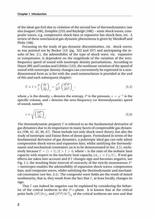
Figure 2.4: Qualitative chart illustrating thermodynamic states that are associ-ated with compression waves that cross the region of negative nonlinearity, i.e.,the region enclosed by the Γ = 0-line and the dew-line, in the P -v-plane. R:Rayleigh line, HR: Hugoniot-Rankine shock adiabat, and s: isentrope. Points Pand Q represent the inflection points of the Hugoniot-Rankine shock adiabat ofstate 1 and point I indicates the inflection point of the isentrope through point 3(or 7).
22

2.2 Compression waves through the BZT-region
[P ] / [v] < (∂P/∂v)HR1,1(which is more stringent than the entropy condition if
the sign of the curvature of isentropes changes [114]), are satisfied. This can beconcluded based solely on the fact that the Rayleigh line connecting states 1 and2 is located completely above the HR shock adiabat of state 1 between points1 and 2. The same arguments also apply to discontinuity 1 → 3 representing asomewhat stronger (becauseP3−P1 > P2−P1) nonclassical compression shockwave, because in this specific situation, the Mach number at the post-shockstate 3 is unity due to the tangency of Rayleigh line R1−3 and HR1,3. Accord-ingly, at state 3, the entropy is a local maximum because
(∂2s/∂v2
)HR1,3
< 0.
Next, consider a configuration represented by jump 1→ 4. Discontinuity 1→ 4however, represents an inadmissible shock wave because the stability criteriumis violated even though the conservation equations are satisfied. Remark thatif point 4 is located very close to point 3 whereby v4 < v3, it is possible thatthe entropy condition is met, namely s4 > s1, however the stability criteriumis violated and the HR shock adiabat is intersected by the Rayleigh line in aninternal point. For jumps whereby the downstream pressure of the wave hasa value between P3 and P4, two situations can arise. In the first situation, thewave disintegrates into a nonclassical compression shock immediately followedby a nonclassical isentropic compression fan. Here the shock wave is nonclas-sical because the post-shock Mach number Ma3 = 1. This occurs because, aswas already shown, the entropy at a post-shock sonic point is a local extremum.Moreover, from thermodynamics it follows that(
∂s
∂P
)v
=ρCP c
2
βPT> 0 (2.37)
signifying that at point 3, the isentrope is located above HR1 and because(∂2s
∂v2
)HR1,3
= −2 [v] c23Γ3
T3v33
, (2.38)
the local extremum in entropy corresponds to a local maximum in entropy.Jump 1 → 7 (whereby the downstream pressure corresponds to P7) representssuch a phenomenon of shock wave splitting; the composite wave consists ofa downstream sonic compression shock wave 1 → 3 and an isentropic com-pression fan 3 → 7. This type of phenomenon arises for downstream pressuresbetweenP3 andPI, where point I is located on the isentrope through point 3 (s3)and the Γ = 0-line. The second situation occurs if the downstream pressure issomewhat greater than PI. If for example the downstream pressure is P8, a non-classical compression shock wave representing jump 1→ 3 is formed (Ma3 = 1),followed by an isentropic nonclassical compression fan, and because the con-vected sound speed decreases with a decrease in specific volume if v < vI, thecompression fan develops a region of multivaluedness, i.e., the high-pressurepart of the wave overtakes the low-pressure part, resulting in the formation of
23

Chapter 2. Nonclassical gas dynamics and Bethe-Zel’dovich-Thompson fluids
a second nonclassical compression shock (the second shock wave is also non-classical because the pre-shock Mach number, Ma7 = 1). Jump 1 → 3 → 7 → 8represents such a shock-fan-shock composite wave. Note that HR shock adia-bat of point 7 is located beneath the isentrope through point 7 (or alternativelypoint 3) and R7−8 is located completely above HR7. For downstream pressurescorresponding to values between PI and P5, composite compressive shock-fan-shock waves are admissible, whereby the pressure jump across the second com-pression shock wave increases as the downstream pressure is increased, whilethe pressure change across the nonclassical compression fan, sandwiched be-tween the two nonclassical compression shock waves, decreases. Line M is thelocus of possible post-shock states of composite waves for downstream pres-sures between PI and P5. Finally, if P = P5, the fan disappears completelyand jump 1 → 5 represents a single compression shock wave or alternatively,jump 1 → 5 can be interpreted as representing a composite wave composedof a compression shock wave (1 → 3, with Ma3 = 1) immediately followed bya second compression shock wave (3 → 5). For higher downstream pressures,e.g., P = P6 only pure classical compression shock waves are admissible.
The previous discussion allows for delimiting the region of pure nonclassicalcompression fans. Making use of the geometrical relations whereby compres-sion shock waves are admissible if and only if the Rayleigh line is located com-pletely above the HR shock adiabat, implies that pure compression fans can begenerated if and only if both the upstream and downstream thermodynamicstates are located within the region of Γ ≤ 0, whereby the up- and downstreamstates are connected via isentropes.
2.3 Expansion waves through the BZT-region
In this section, the focus is on expansion waves that either originate in the re-gion of negative nonlinearity or have an upstream state located on an isen-trope (or HR shock adiabat) that crosses the region of negative nonlinearity.The treatment outlined here summarizes the in-depth analysis of nonclassicalgas-dynamic discontinuities of Kluwick [114] and Zamfirescu et. al. [226]. Withreference to Fig. 2.5, consider a pre-shock state 1 which is located inside thenegative nonlinearity region. Jump 1 → 2 represents an admissible pure non-classical expansion shock wave which satisfies both the entropy inequality andthe mechanical stability condition since the Rayleigh line connecting states 1and 2 is located completely below the HR shock adiabat of state 1 [124]. Simi-larly, jump 1 → 3 represents a possible solution, whereby in this specific situa-tion, the post-shock state is at sonic conditions, i.e., Ma3 = 1, because R1−3 istangent to HR1,3. Moreover, at sonic point 3, the entropy corresponds to a localmaximum. Discontinuity 1 → 4 however, is an inadmissible expansion shockwave because HR1 is intersected by R1−4 approximately at the middle. Never-theless, if the downstream pressure is less than the value corresponding to P3,
24

2.3 Expansion waves through the BZT-region
v
1
2
P
Q
HR1
dew-line
Γ = 0
3
4 4’
R1-2
R1-4
s3 = s4’ > s1 R1-3
P
Figure 2.5: Qualitative chart illustrating thermodynamic states that are associ-ated with expansion waves that originate in and possibly transverse the region ofnegative nonlinearity, i.e., the region enclosed by the Γ = 0-line and the dew-line,in the P -v-plane. R: Rayleigh line, HR: Hugoniot-Rankine shock adiabat, and s:isentrope. Points P and Q represent the inflection points of the Hugoniot-Rankineshock adiabat of state 1; these are in close proximity to the Γ = 0-line.
25

Chapter 2. Nonclassical gas dynamics and Bethe-Zel’dovich-Thompson fluids
1’
v
1
P
Q
Γ = 0
dew-line
M 2
4
5
6’ 5’
R1-5/1-5’
R1-6
HR1’
R1’-2
s6 = s6’ > s1
6
R1-4
s1 = s1’
3 R1-3
P
Figure 2.6: Qualitative chart illustrating thermodynamic states that are associ-ated with expansion waves that cross the region of negative nonlinearity, i.e., theregion enclosed by the Γ = 0-line and the dew-line, in the P -v-plane. R: Rayleighline, HR: Hugoniot-Rankine shock adiabat, and s: isentrope. Points P and Q rep-resent the inflection points of the Hugoniot-Rankine shock adiabat of state 1.
26

2.3 Expansion waves through the BZT-region
v
1 Γ = 0
dew-line
HR1
2
s5 > s1
s1
R1-2
K
P
Figure 2.7: Qualitative chart illustrating thermodynamic states that are associ-ated with double sonic shock waves. The dash-dot-dot line illustrates part of thedouble sonic locus. R: Rayleigh line, HR: Hugoniot-Rankine shock adiabat, ands: isentrope. Point K is the single inflection point of the isentrope through K.
27

Chapter 2. Nonclassical gas dynamics and Bethe-Zel’dovich-Thompson fluids
shock splitting occurs, namely an expansion shock wave is formed connectingstates 1 → 3 with Ma3 = 1; the shock wave is immediately followed by an isen-tropic expansion fan which propagates with the convected sound speed. Anexample of shock splitting of the mentioned type, is indicated by 1 → 3 → 4′ inFig. 2.5.
As a second case, consider an upstream state 1 which is located to the leftof the region of negative nonlinearity on an isentrope that exhibits both convexand concave behavior, see Fig. 2.6. First consider the situation where the down-stream pressure is slightly less that P1 and the specific volume at the down-stream state is less than the value corresponding to the specific volume of theinflection point of the isentrope through point 1, i.e., v1 ≤ vI (point I is notshown). Because expansion shock waves are impossible due to violation of thesecond law of thermodynamics and the stability criterium, the wave necessar-ily evolves as an isentropic expansion fan. However, if v1 > vI and the down-stream pressure has a value of say P2, then, because of a sign-change of Γ, acomposite wave is formed consisting of an isentropic expansion fan, in this ex-ample 1 → 1′, and an expansion shock wave 1′ → 2, whereby Ma1′ = 1. Thismeans that jump 1 → 3 is inadmissible simply because the Rayleigh line con-necting states 1 and 3 is located completely above the HR shock adiabat of state1, therefore the stability criterium is violated, viz. Ma1 < 1. Such a wave, namelyone with a downstream pressure of P3, would evolve as a fan-shock compositewave where the pre-shock Mach number equals unity. Line M in Fig. 2.6 is alocus of post-states of the expansion shock wave of the composite fan-shock-waves. If the downstream pressure is lower than that corresponding to P3, pureexpansion shock waves are still inadmissible because the HR shock adiabat ofstate 1 is intersected in an interior point by the Rayleigh line; instead, the men-tioned composite waves are admitted. However, if the downstream pressurecorresponds to P4, the Rayleigh line connecting states 1 and 4 is located com-pletely below HR1 and the stability and entropy criteria are not violated. Jump1 → 4 is the first pure nonclassical expansion shock wave that is admissiblefrom pre-shock state 1; moreover, Ma1 = 1 because R1−4 is tangent to HR1,1.Also jump 1→ 6 represents an admissible expansion shock wave whereby here,Ma1 > 1 and Ma6 = 1 since at state 6, R1−6 is tangent to HR1,6. For downstreampressures lower than P6, shock splitting occurs because R1−6 intersects HR1 inan internal point. An example of shock splitting is represented by 1 → 6 → 6′
whereby the transformation from state 6 to state 6′ occurs isentropically alonga fan propagating with the convected sound speed.
Apart from shock waves that feature a pre- or post-shock Mach number ofunity, it is also possible to identify states (PA, vA;PB, vB) that display MaA = MaB
= 1. These so-called double-sonic shock waves are expansion shock waves thatfeature the greatest jump in pressure for a given pre-shock state. Moreover, thepre-shock state must be located on an isentrope which displays both convexand concave behavior [43, 226]. Figure 2.7 gives a graphical description of suchan admissible discontinuity in the P -v-plane. Note that the Rayleigh line con-
28

2.3 Expansion waves through the BZT-region
necting states 1 and 2 is located completely below the HR shock adiabat of state1 and that R1−2 is tangent at both state 1 and 2 of the HR shock adiabat. Whatis even more remarkable is that the pre- and post-shock states are both locatedoutside the Γ < 0-region.
In summary, the following can be stated:
1. The uniqueness of both the pre- and post shock sonic points implies thatthere exists a geometrical locus, the so-called double-sonic locus, in theP -v plane connecting these states (see Cramer [43] and Zamfirescu et.al. [226]).
2. All other expansion shock waves that can be admitted along a given isen-trope, have a lower strength (in terms of pressure jump across the shockwave) than the double sonic shock. These single-phase pre-shock statesare located between the double-sonic locus, specifically the dash-dottedline to the left of point K in Fig. 2.7, and the Γ = 0-line, viz. the dashed lineto the right of point K in Fig. 2.7.
3. Expansion shock waves with a pre-shock state located between the double-sonic locus and the Γ = 0-line, as indicated in the previous item, haveboth upper and lower limits for their associated post-shock state. The up-per limit corresponds to the expansion shock wave with sonic pre-shockconditions, e.g., jump 1 → 4 in Fig. 2.6, and the lower bound correspondsto the expansion shock wave with sonic post-shock conditions, like jump1 → 6 in Fig. 2.6. However, expansion shock waves having a pre-shockstate located inside the negative nonlinearity region only have a lowerbound corresponding to shock waves whereby the post-shock conditionsare sonic.
4. The domain delimiting the region of pre-shock states that allow for theadmissibility of nonclassical gas-dynamic phenomena, is bounded by theleft branch of the double sonic locus and the right branch of the Γ = 0-line.8
5. The maximum strength in terms of pressure jump for states inside theafore mentioned domain corresponds to the strength of downstream sonicshock waves.
6. For pre-shock states on the right branch of the Γ = 0-line in the P -v plane,no expansion shock waves are admissible.
Apart from the intensity in terms of the pressure jump across expansionshock waves, it is also possible to identify pre-shock states along selected isen-tropes which display the highest pre-shock Mach number. More specifically,
8According to Fig. 2.7, left and right are considered with respect to point K, which correspondsto the single inflection point of the isentrope through K.
29

Chapter 2. Nonclassical gas dynamics and Bethe-Zel’dovich-Thompson fluids
v [m3/kg]
vR [-]
P[b
ar]
PR
[-]
0.000 0.005 0.010 0.015
0 1 2 3 4
7.0
7.5
8.0
8.5
9.0
9.5
10.0
0.8
0.9
1.0
Tm
ax =400
oC
Vapor-liquidEquilibriumRegion
Single-phasemaximum Machlocus
K
Post-shock States
M
L
N
smin
smax
Figure 2.8: The P -v-thermodynamic plane of D6 (the reduced pressure and spe-cific volume, respectively PR and vR, are determined with respect to their criticalpoint value). Shown are the vapor-liquid-equilibrium (VLE) region, the region ofnegative nonlinearity (highlighted), the maximum isotherm related to the ther-mochemical stability of D6 with respect to stainless steel as the containing ma-terial (dash-dotted line), the isentropes smin and smax (dashed lines), the locusof superheated-vapor thermodynamic states L–K that allow for the highest pre-shock Mach number whereby the post-shock Mach number is unity (these associ-ated post-shock states are located on the dotted-line N–K). Point O according toFig. 2.9 is located on the dew-line somewhat to the right of point L.
the results presented hereinafter establish the existence of a locus of pre-shockstates with the greatest supersonic-to-sonic transition across the shock wave.These results are useful in situations that give rise to unsteady expansion shockwaves, as treated in Chap. 5. In this context, the maximum-Mach-locus is deter-mined for dodecamethylcyclohexasiloxane (D6, [(CH3)2-Si-O]6), which is iden-tified as a BZT fluid in Ref. [30]. Thermodynamic properties of this fluid arecalculated with the EoS documented in Ref. [33] (see also Chap. 3 for details).The procedure is as follows:
30

2.3 Expansion waves through the BZT-region
v [m3/kg]
Ma
[-]
0.004 0.005 0.006 0.007 0.0081.00
1.01
1.02
1.03
MK
L O
Figure 2.9: The pre-shock Mach number, associated with a post-shock Machnumber of unity, as a function of the specific volume along selected isentropesof D6. Thermodynamic properties are determined with the multiparameter EoSdocumented in Ref. [33] (see also Chap. 3). The solid line represents saturated-vapor states featuring a post-shock Mach number of unity, the dotted lines rep-resent isentropes that intersect the dew-line of D6, the dash-dotted lines are isen-tropes that are completely in the superheated-vapor regime, and the dashed lineconnects the maxima of the Ma-v-curves for the latter isentropes. Point O repre-sents the expansion shock wave with the highest possible pre-shock Mach numberwith a sonic post-shock state for D6.
1. For the working fluid, determine the dew-line and the Γ = 0-locus in thedense-gas regime.
2. With reference to Fig. 2.8 compute and draw the isentropes smin and smax.All other isentropes si located in between smin and smax exhibit an intervalof concavity in the dense-gas P -v-thermodynamic plane.
3. Starting from the dew-line for a given isentrope smin ≤ si ≤ smax, de-termine by using the shock admissibility conditions, namely Eqns. (2.17),
31

Chapter 2. Nonclassical gas dynamics and Bethe-Zel’dovich-Thompson fluids
the above-mentioned geometric arguments and the EoS of the fluid, boththe pre-shock Mach number (MaA) whereby the post-shock Mach num-ber MaB = 1, and the pre-shock specific volume vA. Next, increase thespecific volume along the same isentropes si by ∆v and again, for thisnewly assigned pre-shock state, determine MaA with the condition thatMaB = 1.
4. Application of the sequence of calculations outlined in the previous itemresults in the graph displayed in Fig. 2.9 illustrating the pre-shock Machnumber, associated with a post-shock Mach number of unity, as a functionof the pre-shock specific volume along selected isentropes of D6. Fromthis graph it is possible to identify for a given isentrope, a unique single-phase thermodynamic state with the greatest supersonic-to-sonic transi-tion. Connecting these thermodynamic states gives the maximum-Machlocus, as indicated by the line connecting M-L-K in Fig. 2.8 (or the lineconnecting M-L-O-K in Fig. 2.9).
Nomenclature
Symbol Description
A Areab Speed-of-propagation vector of the
shock wave with respect to a laboratoryreference frame
CP Specific isobaric heat capacityCv Specific isochoric heat capacityc Thermodynamic speed of soundDik Rate-of-deformation tensore Specific internal energyF Thermodynamic function defined by
Eq. (2.4) and valid only for isentropicflows
G Gruneisen parameterh Specific enthalpyJ Mass fluxJ Riemann invariant for constant-area
flows with negligible body forcel Variable which appears after a particular
coordinate transformationMa Mach numbern Unit normal vectorP PressureContinued on the next page. . .
32

2.3 Expansion waves through the BZT-region
Continued
Symbol Description
p Unit vector tangential to a control-volume surface
s Specific entropyT Absolute temperaturet Unit vector tangential to a control-
volume surfacet Timeu Fluid velocity vector with respect to a lab-
oratory reference framev Specific volumew Fluid velocity vector with respect to a
shock-related reference framex Spatial coordinatex0 Variable which appears after a particular
coordinate transformation
βP Coefficient of volume expansionΓ Fundamental derivative of gas dynamicsγ Heat capacity ratioε Shock-wave thicknessζ Bulk viscosityη Dynamic (shear) viscosityκ Thermal conductivityλ Second viscosity coefficientρ Densityσ Wave speedτ Time constant related to relaxation phe-
nomenaΦ Dissipation function
33


“They misunderestimated me.”
President George W. Bush, Bentonville, Arkansas, November 6,2000
3Thermodynamic properties of
selected dimethylsiloxanes
Selected contents from:
NANNAN, N. R. AND COLONNA, P. Improvement on multiparameter equations of state for dimethyl-
siloxanes by adopting more accurate ideal-gas isobaric heat capacities: supplementary to P. Colonna,
N. R. Nannan, A. Guardone, and E. W. Lemmon, Fluid Phase Equilib. 244, 193 (2006). Fluid Phase
Equilib. (2009) in press.
COLONNA, P., NANNAN, N. R., AND GUARDONE, A. Multiparameter equations of state for silox-
anes: [(CH3)3-Si-O1/2]2-[O-Si-(CH3)2]i=1...3, and [O-Si-(CH3)2]6. Fluid Phase Equilib. 263, 2 (2008),
115 - 130.
NANNAN, N. R., COLONNA, P., TRACY, C. M., ROWLEY, R. L., AND HURLY, J. J. Ideal-gas heat ca-
pacities of dimethylsiloxanes from speed-of-sound measurements and ab initio calculations. Fluid
Phase Equilib. 257, 1 (2007), 102 - 113.
COLONNA, P., NANNAN, N. R., GUARDONE, A., AND LEMMON, E. W. Multiparameter equations
of state for selected siloxanes. Fluid Phase Equilib. 244, 2 (2006), 193 - 211.
35

Chapter 3. Thermodynamic properties of selected dimethylsiloxanes
Abstract
As is discussed in the subsequent chapters, Chaps. 4–6, the choice of appropri-ate initial conditions as well as the design of an experimental facility that can beused to generate and demonstrate the existence of nonclassical gas-dynamicphenomena, mandates the use and possibly development of good thermody-namic models. A good thermodynamic model in this context refers to its pre-dictive capabilities and to the accuracy with which properties can be computed.The research activities that are documented in the following have been per-formed to obtain a better description of all thermodynamic properties of se-lected linear and cyclic dimethylsiloxanes in the entire range of pressure andtemperature that is of interest for technical applications in general. In par-ticular, this effort has been driven by the needs of the envisaged gas-dynamicexperiment at the Delft University of Technology, see Chap. 6, aimed at prov-ing the existence of nonclassical gas-dynamic phenomena in the thermody-namic region adjacent to the saturated vapor line at high reduced pressuresand temperatures. Siloxanes have been chosen as test fluids, as motivated inSec. 5.6. The selected functional form of the equations of state is that pro-posed by Span and Wagner for nonpolar and weakly polar substances, sincethis modern functional form uses a rather small number of parameters, pro-vides sufficient accuracy from a technical viewpoint and has good extrapolationbehavior. Because of scarcity of experimental thermal and caloric property datafor most of these substances, estimation methods with reasonable uncertainty(∼ 2–5 %) were employed, if necessary, to generate thermal-property data tobe used for optimizing the fluid-specific parameters. Due to the unavailabilityof heat-capacity data however (hexamethyldisiloxane (MM, (CH3)3-Si-O1/2]2)is an exception), and particularly because of the large uncertainty associatedwith ad hoc estimation techniques if applied to organic silicon oils, namely∼ 25 %, a two-pronged approach was used to obtain molar ideal-gas heat capac-ity data (C0
P ) of selected siloxanes. Firstly, acoustic resonance measurementswere made on gas-phase octamethylcyclotetrasiloxane (D4, [(CH3)2-Si-O]4) anddecamethylcyclopentasiloxane (D5, [(CH3)2-Si-O]5) over the temperature range450 K to 510 K. These new experimental data, along with previously publishedmolecular vibrational frequency data for hexamethyldisiloxane, were used todevelop an appropriate frequency scaling factor that can be used with ab ini-tio frequency calculations to determine reliable ideal-gas heat capacities as afunction of temperature. Ideal-gas heat capacities for both cyclic [(CH3)2-Si-O]n (with 3 ≤ n ≤ 8) and linear (CH3)3-Si-O-[(CH3)2-Si-O]n-Si-(CH3)3 (with0 ≤ n ≤ 5) siloxanes over a wide range of temperatures were determined bymeans of ab initio calculations. The collaboration with the process measure-ment division of the National Institute of Standards and Technology (NIST),Gaitherburg, MD and with DIPPR R© thermodynamic properties laboratory atBrigham Young University, Provo, UT is acknowledged.
36

3.1 Introduction
3.1 Introduction
Many energy conversion applications employ organic fluids as working media.Some of these organic compounds and their applications are listed in Table 3.1.Out of the class of organic fluids, siloxanes have many favorable characteristics –they feature good lubricating properties, are odorless, non-toxic, thermochem-ically stable up to high temperatures, scarcely flammable, and in the case oforganic-Rankine-cycle (ORC) applications, these compounds are already em-ployed because they exhibit good thermodynamic properties with respect tocycle design (see e.g., Refs. [7, 4, 6, 5]). Siloxanes are bulk-produced, mainly forthe cosmetics industry. What is more is that, due to their molecular complexity,siloxanes are Bethe-Zel’dovich-Thompson (BZT) fluids [30] (see also Sec. 4.4)and may thus exhibit nonclassical gas-dynamic behavior in the dense-gas re-gion close to saturation at high reduced pressures and temperatures.
Accurate and consistent predictions of thermodynamic properties are of theutmost importance both in the design of advanced process- and energy ap-plications, e.g., high-temperature organic Rankine cycles, supercritical heat-pumps [8], process expanders and compressors in the (petro)chemical indus-try operating in the dense-gas thermodynamic regime [15, 111], as well as innonclassical gas-dynamic investigations. A benchmark analysis documented inChap. 4 shows that, at present, equations of state (EoS’s) are the choice for thelatter. References [37, 4] for example document the use of the Peng-Robinson[161], Stryjek and Vera modified [190], cubic EoS (PRSV) for siloxanes. ThePRSV EoS allows for accurate predictions of vapor-pressures – for nonpolar flu-ids within 2 % of experimental data – and can be used with mixing rules topredict thermodynamic properties of mixtures [35, 4]. Physically based cubicEoS’s however, are inherently rather inaccurate close to the critical region andfor predicting saturated and sub-cooled liquid densities (especially for polarmolecules) [1]. In the case of the PRSV EoS, thermodynamic properties alsodisplay a discontinuity at the critical temperature. With modern equations ofstate however, all thermodynamic properties of technical interest can be cal-culated with high accuracy and are thermodynamically consistent. The consis-tency of the thermodynamic model is a requirement if it is employed in compu-tational fluid dynamics (CFD) programs [37, 35] or in dynamic systems simula-tions [207, 78].
Primarily, the documented work is related to the development of consistenttechnical equations of state for selected linear and cyclic siloxanes useful notonly for nonclassical gas dynamic studies, but also for the design and analysisof technical applications in general. Referring back to the study performed byColonna and Silva [37] where selected siloxanes were identified for the first timeas BZT candidates, it was stated by the latter authors that the greatest sourceof uncertainty in the thermodynamic model was due to the rather large uncer-tainty in the estimation of the ideal-gas isobaric heat capacity, namely 25 %.For this reason, prior to the development of an EoS, as outlined in Sec. 3.3, a
37

Chapter 3. Thermodynamic properties of selected dimethylsiloxanes
Table 3.1: Energy conversion applications of organic fluids.
Fluid family Applications
Hydrocarbons Expanders and compressors in (petro)chemical processes,geothermal organic Rankine cycles (ORC’s)
Fluorocarbons Refrigeration and air conditioning, geothermal ORC’s, lowtemperature heat recovery ORC’s
Siloxanes High temperature ORC’s, heat transfer fluids as mix-tures (possible future application: high-temperature heatpumps)
two-pronged approach was used to obtain accurate molar ideal-gas heat ca-pacity data (C0
P ) of selected siloxanes. Using the new C0P data documented in
Sec. 3.2 which feature an estimated uncertainty of no more than 5–6 %, a mul-tiparameter Helmholtz-energy-based EoS is established for selected siloxaneswhich allows for the prediction of all thermodynamic properties with an accu-racy sufficient for technical applications, e.g., design of ORC engines.
3.2 Ideal-gas isobaric heat capacities of selected lin-ear and cyclic dimethylsiloxanes
3.2.1 Overview
The work presented in this section is aimed at reducing the large uncertainty,namely∼ 25 % according to DIPPR [172], in the estimate of the molar ideal-gasisobaric heat capacity (C0
P ) of linear and cyclic siloxanes. The only estimationmethod which is applicable to this family of fluids is the zeroth-order methodby Harrison and Seaton [86] which was not specifically developed for these flu-ids, hence the large uncertainties. Knowledge of the temperature dependencyof the (molar) ideal-gas isobaric heat capacity is essential for obtaining a com-prehensive thermodynamic model, as discussed in Sec. 3.3.
To achieve the goal, C0P ’s for octamethylcyclotetrasiloxane (D4, [(CH3)2-Si-
O]4) and decamethylcyclopentasiloxane (D5, [(CH3)2-Si-O]5) were determinedusing the acoustic resonance technique. The employed experimental apparatusavailable at NIST limited the temperature range from 450 K to 510 K. Informa-tion from the experiments was used to extend the estimation of C0
P from 298 Kto the compound’s decomposition temperature by using ab initio calculationsand this computational method was also employed to provide estimates of C0
P
for other selected members of the linear- and cyclic-siloxanes family.The structure of this section is as follows: Ssec. 3.2.2 describes the experi-
mental technique that was employed to measure the speed of sound in D4 and
38
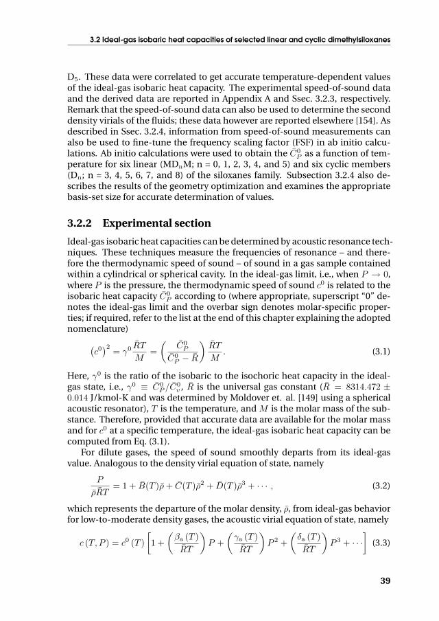
3.2 Ideal-gas isobaric heat capacities of selected linear and cyclic dimethylsiloxanes
D5. These data were correlated to get accurate temperature-dependent valuesof the ideal-gas isobaric heat capacity. The experimental speed-of-sound dataand the derived data are reported in Appendix A and Ssec. 3.2.3, respectively.Remark that the speed-of-sound data can also be used to determine the seconddensity virials of the fluids; these data however are reported elsewhere [154]. Asdescribed in Ssec. 3.2.4, information from speed-of-sound measurements canalso be used to fine-tune the frequency scaling factor (FSF) in ab initio calcu-lations. Ab initio calculations were used to obtain the C0
P as a function of tem-perature for six linear (MDnM; n = 0, 1, 2, 3, 4, and 5) and six cyclic members(Dn; n = 3, 4, 5, 6, 7, and 8) of the siloxanes family. Subsection 3.2.4 also de-scribes the results of the geometry optimization and examines the appropriatebasis-set size for accurate determination of values.
3.2.2 Experimental section
Ideal-gas isobaric heat capacities can be determined by acoustic resonance tech-niques. These techniques measure the frequencies of resonance – and there-fore the thermodynamic speed of sound – of sound in a gas sample containedwithin a cylindrical or spherical cavity. In the ideal-gas limit, i.e., when P → 0,where P is the pressure, the thermodynamic speed of sound c0 is related to theisobaric heat capacity C0
P according to (where appropriate, superscript “0” de-notes the ideal-gas limit and the overbar sign denotes molar-specific proper-ties; if required, refer to the list at the end of this chapter explaining the adoptednomenclature)(
c0)2
= γ0 RT
M=(
C0P
C0P − R
)RT
M. (3.1)
Here, γ0 is the ratio of the isobaric to the isochoric heat capacity in the ideal-gas state, i.e., γ0 ≡ C0
P /C0v , R is the universal gas constant (R = 8314.472 ±
0.014 J/kmol-K and was determined by Moldover et. al. [149] using a sphericalacoustic resonator), T is the temperature, and M is the molar mass of the sub-stance. Therefore, provided that accurate data are available for the molar massand for c0 at a specific temperature, the ideal-gas isobaric heat capacity can becomputed from Eq. (3.1).
For dilute gases, the speed of sound smoothly departs from its ideal-gasvalue. Analogous to the density virial equation of state, namely
P
ρRT= 1 + B(T )ρ+ C(T )ρ2 + D(T )ρ3 + · · · , (3.2)
which represents the departure of the molar density, ρ, from ideal-gas behaviorfor low-to-moderate density gases, the acoustic virial equation of state, namely
c (T, P ) = c0 (T )[1 +
(βa (T )RT
)P +
(γa (T )RT
)P 2 +
(δa (T )RT
)P 3 + · · ·
](3.3)
39

Chapter 3. Thermodynamic properties of selected dimethylsiloxanes
represents the speed of sound in dilute gases as a function of temperature andpressure. In Eq. (3.3), βa (T ), γa (T ), and δa (T ) are the second, third, and fourthacoustic virial coefficients, respectively. These only depend on the temperatureas do the corresponding (density) virial coefficients B (T ), C (T ), and D (T ) inEq. (3.2). The second acoustic virial and the second density virial are connectedby the thermodynamic relation
βa (T ) = 2B (T ) + 2(γ0 − 1
)TdB (T )dT
+
(γ0 − 1
)2γ0
T 2 d2B (T )dT 2
. (3.4)
Expressions relating the higher-order acoustic virials to the higher-order densityvirials are also available [77, 76].
Values for the acoustic virial coefficients and the ideal-gas speed of soundare obtained by fitting Eq. (3.3) to experimental speed-of-sound and pressuredata along isotherms. From the fitted values of c0 (T ), the ideal-gas isobaricheat capacity can be determined from
C0P =
(c0)2M
T[(c0)2
M/RT − 1
] . (3.5)
A detailed description of the experimental equipment is given by Gillis [76].In the following only a brief description of the resonator and of the measure-ment procedure is given.
3.2.2.1 The resonator
The resonator that was used for resonance frequency measurements was a cylin-der with circular cross-section and was fabricated of a copper-nickel alloy. Theheight was approximately 14 cm and the width was about 6.5 cm (see Fig. 3.1).The internal surface of the resonator was polished to a mirror finish, therefore,the flat surface area was accurately known. To achieve good temperature stabil-ity and fast temperature equilibration, the cylinder was completely submergedin a continuously stirred liquid bath. This thermostated bath guaranteed thatthe temperature fluctuations in the gas sample were within 1 mK. The top plateof the cylinder contained a carefully designed port for charging and removalof the sample. The electro-acoustic transducers, these are the sound sourceand the microphone detector, were remote from the resonator because the hightemperature of the thermostated bath was not compatible with these trans-ducers. Instead, the sound waves generated at (received by) the source (mi-crophone detector), were carried to (from) the resonator by waveguides. Thewaveguides are hollow cylindrical tubes with horn-shaped cross sections andwere filled with argon. Apart from protecting the electro-acoustic transducersfrom the harsh environment of the thermostated bath and the gas in the res-onator, the physical separation of the transducers by the waveguides reduces
40

3.2 Ideal-gas isobaric heat capacities of selected linear and cyclic dimethylsiloxanes
Figure 3.1: Schematic representation of the cylindrical resonator, the waveguides,and the electro-acoustic transducers (adapted from Ref. [76]). E: sound emit-ter, D: sound detector, R: resonator, and PRT: standard platinum resistance ther-mometer.
electro-magnetic and mechanical disturbances between the sound source andthe microphone detector. A metal membrane separated the argon in the waveg-uides from the siloxane sample. To weaken resonances in the waveguides, whichmay complicate the resonance-frequency measurements in the sample, a metalscreen was placed in both waveguides near the metallic membrane. The pres-sure of the sample was measured with a quartz-bourdon-tube pressure gauge inconjunction with a diaphragm-type differential pressure transducer (DPT). Thepressure gauge measured the pressure of argon in the waveguides and the DPT,which was always kept at 230 oC, measured the pressure difference between theargon and the sample. To avoid pre-condensation,1 the pressure of the test fluid
1this is a phenomenon whereby, if the thermodynamic state of the test fluid is close to satura-tion, evaporation and condensation occur at the resonator walls as a consequence of pressure andtemperature variations caused by the acoustic cycle [142].
41

Chapter 3. Thermodynamic properties of selected dimethylsiloxanes
was kept to 80 % of the vapor pressure of the sample at the bath temperature orto that corresponding to 230 oC, whichever was lower. At the highest temper-ature that was reached, the DPT was relatively colder, so that was the limitingtemperature.
3.2.2.2 Sample purity
A major source of uncertainty in C0P derived from speed-of-sound data is sam-
ple impurity. For small levels of impurity, the fractional uncertainty in the de-rived ideal-gas isobaric heat capacity is approximately:
σu(C0P,t
)C0P,t
≈
(C0P,i
C0P,t
− 1
)︸ ︷︷ ︸
first term
+(Mi
Mt− 1)
1(γ0
t − 1)︸ ︷︷ ︸second term
ι+O(ι2). (3.6)
Subscripts “t” and “i” denote the fluid sample and the impurity, respectively,σu ( ) represents the absolute uncertainty of the property between the roundbrackets, and ι denotes the mole fraction of impurity in the sample. The terminvolving the ratio of the isobaric heat capacity of the impurity and that of thesample is usually small compared to the second term in Eq. (3.6). Complex flu-ids with many active vibrational degrees of freedom at the temperature of inter-est have large heat capacities and heat-capacity ratios, γ0
t , very close to unity.For example, γ0
t ≈ 1.017 for D4 at 500 K if C0P is estimated using the Harrison-
Seaton method. This means that if the D4 sample contains impurities for which(Mi/Mt − 1) is of the order of unity, the fractional uncertainty in C0
P,t is of theorder of 50 times the mole fraction of the impurity.
The test fluids were octamethylcyclotetrasiloxane (D4, [(CH3)2-Si-O]4) anddecamethylcyclopentasiloxane (D5, [(CH3)2-Si-O]5) and had been supplied bythe European branch of the Tokyo Chemical Industry Co, Ltd. These fluids wererated by the manufacturer as 99.9+ % pure; no gas-chromatographic analysiswas done. The impurities that were present were most likely other siloxanes.Before the fluids were loaded into the resonator, they were thoroughly degassedto remove air and other volatilities by repeatedly freezing the fluid in liquid ni-trogen and evacuating the space above the frozen sample.
3.2.2.3 Calibration
For accurate speed-of-sound measurements, the resonator needs to be cali-brated. Calibration is necessary for determining the temperature-dependentdimensions of the cylinder. This was achieved by measuring the frequenciesof resonance of different acoustic modes in argon in the temperature and pres-sure range of interest. Argon was chosen for the calibration, because it is inert
42

3.2 Ideal-gas isobaric heat capacities of selected linear and cyclic dimethylsiloxanes
and because its transport properties and speed of sound are known with highaccuracy.
For the cylinder that was used to measure the sound speed in the siloxanes,the following dimensions were obtained for temperatures between 350 K and500 K:
L = L0 [1 + α (T − T0)] . (3.7)
Here, L0 denotes the length of the cylinder at the reference temperature T0 =273.15 K. From measurements with argon, it was inferred that L0 equals 14.04 cm.The thermal expansion coefficient of the copper-nickel alloy was assumed tohave a power-law dependence with temperature, i.e., α ∝ TB, whereby the pro-portionality constant was found to be equal to 1.184 · 104 K−B−1 and B = 1.866([α] = K−1 ). The radius had the following temperature dependence:
R = R0 [1 + α (T − T0)] . (3.8)
The radius R0 at T0 = 273.15 K was determined from the calibration run withargon. From the obtained data it was inferred that R0 equals 3.279 cm. All pres-sure and temperature transducers were calibrated only once.
3.2.2.4 Measurement procedure
The measurement procedure was as follows:
- At first, the thermostated bath was set to the desired measurement tem-perature. Once this temperature was reached, the resonator was chargedwith the gas sample. Acoustic measurements were made at pressures upto 80 % of the vapor-pressure at the thermostated temperature of eitherthe bath or the DPT, whichever was lower. At pressures closer to the dewpoint, condensation at the walls due to the acoustic cycle can become aproblem. This so-called pre-condensation lowers the apparent speed ofsound [142]. The vapor-pressure was determined from the AIChE DIPPR R©equation [172] using the substance specific parameters for the siloxanesD4 and D5, given by Flaningam [69].
- After the temperature of the gas sample had equilibrated, selected purelylongitudinal modes and one purely radial mode were measured. Redun-dant measurements were conducted to give confidence that the correctmodes were measured. Because of the low speed of sound, it is impor-tant for the siloxanes considered herein to distinguish between pure andmixed modes. For example, the first purely longitudinal mode for D4 at450 K occurs at a frequency of about 380 Hz. Because the experimen-tal equipment (resonator and transducers) was not specifically designed(selected) to measure frequencies significantly below 1 kHz, it was nec-essary to measure higher modes (at low frequencies the signal to noise
43

Chapter 3. Thermodynamic properties of selected dimethylsiloxanes
ratio is small). Higher modes however, are spaced closer to each otherthan are, for example, the first and second purely longitudinal mode. It istherefore important to do redundant measurements in order to check (butalso to distinguish) which modes are measured and whether they are puremodes or mixed modes. Additionally, redundant modes give a measure ofthe uncertainty in the resonance frequency f . To account for first-orderdrifts that can occur in temperature and pressure during a measurementcycle, each resonance frequency was measured three times. Furthermore,at each measurement, the interval sweep of the scan was in two direc-tions, i.e., from f − g to f + g and then back from f + g to f − g. Here, g isthe experimentally determined half-width, i.e., the width of the resonancefrequency at 2−1/2-times the signal’s maximum amplitude. Known con-tributions to the half-width (loss mechanisms) are: i) sound absorptionat the metal-gas boundaries due to the formation of thermal and viscousboundary layers, ii) sound absorption in the bulk of the fluid as a conse-quence of the local rate of compression and fluid friction, iii) irreversibleheat flows in the bulk of the fluid due to the periodic changes in temper-ature during the acoustic cycle, and iv) imperfections in the cylinder suchas the fill duct and the gap at the O-ring seal.
- After the measurement sequence for each thermodynamic state, the pres-sure was reduced by about 10 kPa while the temperature was kept con-stant. Once pressure and temperature equilibrated (this required about5 minutes), the resonance frequencies were measured again. The detectedresponse of the measured resonance frequency is pressure dependent andattenuates with decreasing pressure. Consequently, the lowest pressure atwhich resonance frequencies were measured was 22 kPa.
3.2.3 Experimental results
3.2.3.1 Experimental data for D4
The speed of sound in D4 was measured along the isotherms of 450 K, 465 K,480 K, and 495 K. The lower temperature limit was chosen based on the fact thatfor good speed-of-sound measurements in this apparatus, the pressure of thesample should approximately be greater than 30 kPa and less than about 80 %of the vapor pressure at the temperature of measurement. At lower pressuresthe signal-to-noise ratio is small and therefore it is difficult to measure the reso-nance frequency. The upper temperature limit is determined by the maximumallowed temperature of the liquid used in the thermostated bath and the high-est temperature at which the DPT can operate.2 The pressure spanned the range
2There is also an upper density limit: if superheated vapor densities are of the order of the criticaldensity, speed-of-sound data determined with the acoustic resonance technique are not very accu-rate because of an increase of the coupling of the oscillations of the vapor enclosed in the resonator
44

3.2 Ideal-gas isobaric heat capacities of selected linear and cyclic dimethylsiloxanes
Table 3.2: Derived values for the ideal-gas speed of sound and isobaric heat ca-pacity of D4.
T [K] c0 [m/s] σu(c0)/c0 [%] C0P [J/mol-K] σu(C0
P )/C0P [%]
450 113.3 0.014 469.5 1.6465 115.2 0.041 480.6 4.7480 117.0 0.019 491.8 2.2495 118.8 0.060 503.0 7.1
27 kPa - 225 kPa. The measured modes included the 5th and 7th purely longitu-dinal mode and the 1st purely radial mode. The experimental resonance fre-quency f exp is slightly lower than the ideal resonance frequency f from whichthe true speed of sound should be determined. The shift in frequency, ∆f , isthe result of the viscous and thermal boundary layers at the walls of the res-onator. The shift in frequency depends on the transport properties of the fluidsample, namely the shear viscosity, the bulk viscosity, and the thermal conduc-tivity. Trusler [205] gives relevant equations that should be used to compute thefrequency shift ∆f ; moreover, ∆f is related in part to the experimentally mea-sured half-width of the signal (note that irreversible processes in the bulk of thesample contribute to the experimental half-width of a resonance frequency butare not responsible for the frequency shift). Because of the large uncertainty intransport-property estimates for siloxanes [172], this study uses the followingsimple correlation to determine the ideal resonance frequency:
f = f exp + gexp, (3.9)
where gexp denotes the half-width obtained from the measurements.The speed-of-sound data obtained from these frequencies/modes were fit-
ted to the acoustic virial equation of state, Eq. (3.3), to obtain the second andthird acoustic virial coefficient at every temperature. Using the relationship be-tween the second acoustic virial and the second density virial, as expressed byEq. (3.4), values were also obtained for B at the four temperatures [154]. Fromthe speed-of-sound data, ideal-gas isobaric heat capacities were derived. Be-cause of the relatively small temperature range of measurement, it was assumedthat C0
P has a linear dependence on temperature. Table A.1 lists the experimen-tal speed-of-sound data together with the uncertainties in c and Table 3.2 givesthe derived c0’s and ideal-gas isobaric heat capacities at each temperature ofmeasurement. The uncertainties are calculated using the method documentedby Taylor [195].
and the oscillations of the shell enclosing the vapor. Here, the upper density limit was not reached.
45

Chapter 3. Thermodynamic properties of selected dimethylsiloxanes
Table 3.3: Derived values for the ideal-gas speed of sound and isobaric heat ca-pacity of D5.
T [K] c0 [m/s] σu(c0)/c0 [%] C0P [J/mol-K] σu(C0
P )/C0P [%]
485 105.1 0.025 563.3 3.3500 106.7 0.042 574.5 5.7510 107.7 0.054 581.9 7.5
The experimental C0P data, which on average have a predicted experimen-
tal uncertainty of 3.9 %, are compared with the estimates determined from theHarrison-Seaton method. It is observed that the experimental C0
P ’s are withinthe uncertainty assigned by DIPPR R© [172]. Moreover, within the experimentaltemperature range, i.e., 450K < T < 495K, the Harrison-Seaton method givesvalues which are lower than the experimentally derived data by approximately4 %.
3.2.3.2 Experimental data for D5
The speed of sound in D5 was measured along the isotherms of 485 K, 500 K,and 510 K. The pressure spanned the range 22 kPa - 117 kPa. The measuredmodes were again the 5th and 7th purely longitudinal mode and the 1st purelyradial mode. These experimental frequencies were corrected using Eq. (3.9).The speed-of-sound data and the experimental uncertainties are given in Ta-ble A.2 and the derived c0’s and ideal-gas isobaric heat capacities are presentedin Table 3.3. A comparison of the experimentally determined ideal-gas isobaricheat capacities (these have an average experimental uncertainty of 5.5 %) withestimates obtained from the Harrison Seaton method shows that although theexperimental C0
P ’s are within the uncertainty of the group-contribution method[172], the experimental C0
P ’s are lower than values determined from the methodof Harrison and Seaton and values obtained from the ab initio calculations (seeTable 3.7). This is contrary to what was observed for D4. This discrepancy is apossible consequence of impurities in the D5 sample: since the same resonatorwas used for resonance frequency measurements in both fluids, it is reasonableto assume that minute amounts of D4 were present during the measurements inD5. This reasoning is consistent, since a lighter constituent in the sample of D5
means that the speed of sound is greater with respect to a measurement not af-fected by impurities. Moreover, using Eq. (3.6) it is found that 0.07 % of D4 as animpurity in D5, reduces the ideal-gas isobaric heat capacity by as much as 1 %.This level of impurity could have been measured using gas-chromatography(GC). However, no GC analyzer with the required sensitivity was available in thelaboratory, therefore it was impossible to check whether cross-contamination
46

3.2 Ideal-gas isobaric heat capacities of selected linear and cyclic dimethylsiloxanes
due to incomplete clean-out of the resonator had occurred. What is even moreimportant is that only after the results from the ab initio computations becameavailable, did it become a point of concern that contamination of the D5 samplemight have happened.
Remark that since the ideal-gas heat capacity ratio is close to unity, the pres-ence of impurities can greatly influence the uncertainty in derived ideal-gas iso-baric heat capacities. Furthermore, due to the low volatility of the siloxanes, theexperiment had to be conducted at high temperatures. A viable approach toobtain accurate C0
P ’s is the use of a buffer gas, e.g., argon, for which accuratethermodynamic properties are available. By measuring the shift in resonancefrequency due to the addition of a small, but accurately known amount of silox-ane in the buffer gas, one can obtain the value of the ideal-gas heat capacityratio of the argon-siloxane mixture, from which C0
P of the siloxane can be de-termined. This approach has been used by Colgate et. al. [26] for measuringC0P ’s of n-butane, isobutane, and n-heptane. This technique will be considered
for possible developments of this work, but it could not be adopted at the timeof the measurements herewith documented because the available cylindricalresonator was not suitable and several modifications would have to be imple-mented.
3.2.4 Ab initio calculations
Several different families of siloxanes have been successfully studied with abinitio methods to help elucidate the relatively flexible Si-O backbone structurethat is largely responsible for many of their useful properties [70]. Previousstudies show that the Si-O bond is relatively short. This has been attributedto the high ionic character of the bond [90] and to partial transfer of electroniccharge from the O lone electron pair to the Si atom [70]. The bending forceconstant for the Si-O-Si bond angle is very small, and the angle varies between140–180o [70, 91, 68] for different molecules. For example, using HF calcula-tions with modest basis sets for cyclo-n-trisilicic acids, Hill and Sauer [91] foundSi-O-Si angles of 163.6o, 178.6o, and 166.4o for the n = 4, 5, and 6 rings, respec-tively. Freire et. al. [70] found considerable differences in the stable geometriesof dimethyl- and diphenylsiloxane chains. The torsional barriers for rotationsabout the Si-O bonds are also quite low [70]. Thermodynamic measurementshave shown that internal rotation about the Si-O bond in hexamethyldisiloxane(MM, [(CH3)3-Si-O1/2]2) is free, or nearly so [177]. Other experimental results,such as X-ray and electron diffraction [116], also agree quite well with the bondlengths and angles obtained from ab initio calculations.
The use of higher levels of theory and larger basis sets has been limited bythe molecular size of these molecules and the number of electrons involved.However, Kudo et. al. [116] used 6-31G* and 6-311G(d,p) basis sets with bothHF and MP2 calculations for specific conformations of (H2-Si-O)n with n = 3, 4,5. In most cases, the optimized geometries and energies were similar for the HF
47

Chapter 3. Thermodynamic properties of selected dimethylsiloxanes
and MP2 calculations, though the MP2 inclusion of electron correlation effectschanged the stability order of some conformations of nearly equal energies.
Previous ideal-gas-heat-capacity determinations from ab initio frequencycalculations on the siloxane family have not been found in the literature. In thisstudy HF calculations were applied with basis sets similar to those used by Kudoet. al. on the dihydride siloxanes. The convergence of calculated C0
P values isinitially determined with basis set size for MM. This basis set is then used for thegeometry optimization and frequency calculations on twelve of the moleculesstudied here.
3.2.4.1 Basis-set dependence
The ideal-gas isobaric heat capacity is related to harmonic characteristic vibra-tional temperatures, Θj , within the molecule by [171]
C0P
R= 4 +
3m−6∑j=1
(Θj
T
)2{
exp (Θj/T )[exp (Θj/T )− 1]2
}, (3.10)
where m is the number of atoms in the molecule and Θj is related to the in-tramolecular vibrational frequencies, νj , by
Θj =hPνjkB
. (3.11)
Here hP and kB are Planck’s and Boltzmann’s constant, respectively. The deriva-tion of Eq. (3.10) also assumes independence of the rotational and vibrationalmodes.
In this work, harmonic frequencies for the optimized geometry were ob-tained from frequency calculations using Gaussian 98 [73], and these were usedin Eq. (3.10) to obtain C0
P values. Frequencies determined from ab initio calcu-lations may differ from those measured experimentally due to the incompleteinclusion of electron correlation effects and the use of finite basis sets. In allcases, the same basis set was used for the frequency and optimization calcula-tions, but C0
P values for MM were generated using increasingly larger basis setsto determine convergence of C0
P with the number of basis functions employed.MM is the only compound of those studied for which experimental frequencyinformation is available [177]. The basis sets used and the corresponding num-ber of basis functions are given in Table 3.4. While the 3-21G basis set is toosmall for accurate C0
P calculations, acceptable convergence is obtained for 6-31G(d) and larger basis sets. The addition of diffuse functions tends to lower C0
P
values for the double zeta basis sets, but the use of 6-31G(d) gives values con-sistent with the largest basis set studied. HF/6-31G(d) and HF/6-31+G(d) wereused for all subsequent calculations.
Geometry optimizations and frequency calculations were made using HF/6-31G(d) and HF/6-31+G(d) for six linear MDnM siloxanes (0 ≤ n ≤ 5) and for six
48
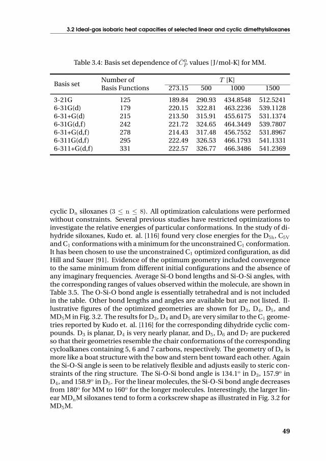
3.2 Ideal-gas isobaric heat capacities of selected linear and cyclic dimethylsiloxanes
Table 3.4: Basis set dependence of C0P values [J/mol-K] for MM.
Basis setNumber ofBasis Functions
T [K]273.15 500 1000 1500
3-21G 125 189.84 290.93 434.8548 512.52416-31G(d) 179 220.15 322.81 463.2236 539.11286-31+G(d) 215 213.50 315.91 455.6175 531.13746-31G(d,f) 242 221.72 324.65 464.3449 539.78076-31+G(d,f) 278 214.43 317.48 456.7552 531.89676-311G(d,f) 295 222.49 326.53 466.1793 541.13316-311+G(d,f) 331 222.57 326.77 466.3486 541.2369
cyclic Dn siloxanes (3 ≤ n ≤ 8). All optimization calculations were performedwithout constraints. Several previous studies have restricted optimizations toinvestigate the relative energies of particular conformations. In the study of di-hydride siloxanes, Kudo et. al. [116] found very close energies for the D5h, C5V
and C1 conformations with a minimum for the unconstrained C1 conformation.It has been chosen to use the unconstrained C1 optimized configuration, as didHill and Sauer [91]. Evidence of the optimum geometry included convergenceto the same minimum from different initial configurations and the absence ofany imaginary frequencies. Average Si-O bond lengths and Si-O-Si angles, withthe corresponding ranges of values observed within the molecule, are shown inTable 3.5. The O-Si-O bond angle is essentially tetrahedral and is not includedin the table. Other bond lengths and angles are available but are not listed. Il-lustrative figures of the optimized geometries are shown for D3, D4, D5, andMD5M in Fig. 3.2. The results for D3, D4 and D5 are very similar to the C1 geome-tries reported by Kudo et. al. [116] for the corresponding dihydride cyclic com-pounds. D3 is planar, D4 is very nearly planar, and D5, D6 and D7 are puckeredso that their geometries resemble the chair conformations of the correspondingcycloalkanes containing 5, 6 and 7 carbons, respectively. The geometry of D8 ismore like a boat structure with the bow and stern bent toward each other. Againthe Si-O-Si angle is seen to be relatively flexible and adjusts easily to steric con-straints of the ring structure. The Si-O-Si bond angle is 134.1o in D3, 157.9o inD4, and 158.9o in D5. For the linear molecules, the Si-O-Si bond angle decreasesfrom 180o for MM to 160o for the longer molecules. Interestingly, the larger lin-ear MDnM siloxanes tend to form a corkscrew shape as illustrated in Fig. 3.2 forMD5M.
49

Chapter 3. Thermodynamic properties of selected dimethylsiloxanes
Table 3.5: Backbone Si-O bond lengths and Si-O-Si angles in the optimizedgeometries showing the average (Ave.) values and the minimum (Min.) andmaximum (Max.) values within the molecule.
SiloxaneSi-O Bond [A= 10−10 m] Si-O-Si Angle [o]Ave. Min. Max. Ave. Min. Max.
LinearMM 1.635 – – 180.00 – –MDM 1.631 1.625 1.637 178.35 178.35 178.35MD2M 1.630 1.625 1.639 168.65 168.47 169.01MD3M 1.633 1.627 1.645 161.16 154.08 168.96MD4M 1.633 1.626 1.643 160.06 158.76 160.77MD5M 1.633 1.627 1.644 159.57 154.81 164.89
CyclicD3 1.648 – – 134.05 – –D4 1.633 – – 157.86 – –D5 1.632 1.630 1.635 158.90 153.95 167.35D6 1.632 1.632 1.633 157.55 154.97 160.51D7 1.631 1.629 1.634 159.48 154.65 163.28D8 1.632 1.627 1.635 157.94 152.93 163.60
3.2.4.2 Frequency scaling factor
Currently, the determination of high-accuracy C0P values from ab initio calcula-
tions requires use of an empirically determined frequency scaling factor (FSF)that adjusts harmonic frequencies, for use in Eq. (3.10), closer to the actual val-ues. In so doing, it is assumed that the scaling factors compensate for anhar-monic effects, errors resulting from the electronic structure calculations, andany lack of complete independence between vibrational and rotational modes.It has been found that such scaling factors are relatively uniform for specificcombinations of theory and basis set, and considerable effort in obtaining FSFvalues is evident in the literature. Early on, Pople at. al [165] proposed an FSFof 0.89 for HF/3-21G, Hout and coworkers [96] suggested an FSF of 0.921 forMP2/6-31G(d), and DeFrees and McLean [52] recommended values of 0.96 forfirst-row molecules and 0.94 for second-row molecules. More recently, Scottand Radom [176] developed and tabulated FSF’s for a large number of modelchemistries. They recommend FSF = 0.8953 for HF/6-31G(d) and FSF = 0.8970for HF/6-31+G(d). More recently Irikura at. al [101] reported an analysis of scal-ing factors based on 358 molecules using the Computational Chemistry Com-parison and Benchmark Database (CCCBDB) maintained by the National Insti-tute of Standards and Technology (NIST). These authors also performed careful
50

3.2 Ideal-gas isobaric heat capacities of selected linear and cyclic dimethylsiloxanes
(a) D3 (b) D4
(c) D5 (d) MD5M
Figure 3.2: Optimized structures of some of the considered siloxanes.
51

Chapter 3. Thermodynamic properties of selected dimethylsiloxanes
Table 3.6: Recommended FSF values for siloxanes.
Compound HF/6-31G(d) HF/6-31+G(d) MP2/6-31+G(d)
MM 1.0316 0.9898 1.0381D4 1.0324 1.0077 –
Average 1.0320 0.9988 –
statistical analysis of the resultant frequency factors and determined uncertain-ties of their recommended values.
Because tabulated FSF values have been based on organic molecules con-taining primarily first- and second-row elements, it is unclear how effectivethese values are in correlation and prediction of siloxane thermochemical prop-erties. Therefore, FSF values for siloxanes appropriate for the basis sets used inthis work have been regressed from the experimental C0
P values for D4 and fromavailable thermochemical data for MM [177]. The resulting values, shown in Ta-ble 3.6, are consistent between the two compounds but closer to unity than thecorresponding FSF values employed for non-Si compounds. The average val-ues shown in Table 3.6 are used throughout this work to predict C0
P values forall of the remaining siloxanes. As an indication of possible electron correlationeffects on the FSF, MP2/6-31+G(d) calculations on MM were also performed.The resultant C0
P ’s were in excellent agreement with experimental values withan optimized FSF = 1.0381.
As mentioned, the FSF scaling of the frequencies attempts to compensatefor deviations from the theoretical model. In this case these include deviationsnot only due to anharmonicity effects and mode coupling effects, but also devi-ations in C0
P due to the modeling of the fluid with the optimized geometry. Thereal fluid will be an equilibrium mixture of molecular conformers, but calcula-tions of C0
P for a couple of different conformations indicates that the variationin C0
P values amongst conformers is likely very small and adequately accountedfor by using the FSF.
3.2.4.3 Predicted ideal-gas isobaric heat capacities
Frequencies were obtained for the six linear and six cyclic siloxanes, adjustedusing the average FSF shown in Table 3.6, and used with Eqns. (3.10) and (3.11)to obtain the values given in Table 3.7 at various temperatures. The listed valuesare predicted and, of course, only apply to the real-gas phase up to tempera-tures at which the fluids thermochemically decompose. Several low-frequencymodes associated with Si-O-Si angle bending were consistent with the knownflexibility of this angle. Similar calculations were made using HF/6-31+G(d) for
52

3.2 Ideal-gas isobaric heat capacities of selected linear and cyclic dimethylsiloxanes
Table 3.7: C0P values [J/mol-K] predicted for linear and cyclic siloxanes using
HF/6-31G(d). Values given for temperatures above the decomposition temper-atures are hypothetical.
FluidT [K]
298 300 400 500 600 700 800 900 1000 1200
LinearMM 232 234 281 323 359 390 418 442 463 499MDM 330 331 397 455 505 547 584 617 646 694MD2M 403 405 489 562 625 679 726 767 804 865MD3M 524 526 629 719 795 881 918 968 1012 1085MD4M 621 624 745 851 941 1018 1084 1143 1194 1280MD5M 718 721 861 983 1086 1174 1251 1318 1377 1476
CyclicD3 273 274 331 379 420 454 484 509 532 570D4 364 365 439 503 557 602 641 676 706 756D5 469 471 564 643 710 768 817 860 897 960D6 566 568 680 775 856 925 984 1035 1080 1155D7 663 666 796 907 1001 1081 1150 1210 1263 1351D8 759 762 911 1039 1146 1238 1317 1385 1446 1546
three MDnM and three Dn compounds, and these results are shown in Table 3.8.Results are similar for the two basis sets although the predicted values are oftenslightly higher with the use of diffuse functions on the heavier nuclei. Figure 3.3compares the D4 experimental values measured here to the ab initio values pre-dicted using the recommended average FSF value developed previously.
Figure 3.4 compares the experimental results for D4 (see Ssec. 3.2.3.1) withvalues predicted by other means. Values predicted using the simple Harrison-Seaton group-contribution method are in very good agreement with the ab ini-tio predicted values over the whole temperature range. Also shown in this figureare values of C0
P estimated using the approximate relationship,
C0P ≈ CL
P +(dHvp
dT
)sat
(3.12)
with values for the saturated-liquid isobaric heat capacity, CLP , and the molar-
specific enthalpy of vaporization, Hvp, obtained from the recommended corre-lations in the DIPPR R© database [172]. Equation (3.12) neglects non-ideal va-por correction terms which can be significant at lower temperatures where theliquid heat capacity is usually more accurately known. Additionally, the corre-lation for Hvp was obtained from the vapor pressure curve using the Clapey-
53

Chapter 3. Thermodynamic properties of selected dimethylsiloxanes
Table 3.8: C0P values [J/mol-K] predicted for selected linear and cyclic siloxanes
using HF/6-31+G(d). Values given for temperatures above the individualdecomposition temperatures are hypothetical.
FluidT [K]
298 300 400 500 600 700 800 900 1000 1200
LinearMM 231 232 280 322 358 390 417 441 462 498MDM 338 339 406 465 515 557 594 627 656 704MD3M 537 539 644 734 811 876 933 983 1026 1099
CyclicD3 279 280 338 387 428 462 491 517 539 576D4 364 366 441 506 559 605 644 678 708 758D5 472 474 568 648 716 773 822 864 902 963
ron equation. This means that the second term in Eq. (3.12) is obtained from asecond-order derivative of the experimental vapor-pressure data. Errors associ-ated with this approximation are also worse at lower temperatures. One wouldtherefore expect this approximate thermodynamic consistency check to be bet-ter at higher temperatures.
Within the accuracy of this test, Fig. 3.4 shows agreement with the availablerelated thermodynamic data. A similar comparison of the ab initio results withthe Harrison-Seaton method and the approximate thermodynamic consistencycheck of Eq. (3.12) was made for the other eleven siloxanes with results simi-lar to those displayed in Fig. 3.5 for MM, MD3M, MD5M, and D5. Agreement ofthe ab initio values is within the expected uncertainty of the approximate ther-modynamic consistency test. The Harrison-Seaton predictions exhibit similartrends, but they are often lower than the ab initio values.
The discrepancy between the measured D5 values (see Ssec. 3.2.3.2) and theab initio predictions is interesting. The thermodynamic consistency check alsoexhibits deviations from the ab initio results. These differences may be due tothe difficulty in purifying D5 and the large effect small amounts of impuritieshave on the speed-of-sound measurements as discussed in Ssec. 3.2.2.2.
54

3.3 Equations of state for selected linear and cyclic siloxanes
T [K]
CP0x
M[J
/mol
-K]
440 460 480 500 520460
480
500
520
Figure 3.3: Experimental C0P values for D4 ( ) compared to ab intio values pre-
dicted by HF/6-31G(d) (solid line) and HF/6-31+G(d) (dashed line) calculationsusing the recommended FSF.
3.3 Equations of state for selected linear and cyclicsiloxanes
3.3.1 Introduction
This section documents the development of short technical multiparameter EoS’sfor:
1. hexamethyldisiloxane (MM, [(CH3)3-Si-O1/2]2),
2. octamethyltrisiloxane (MDM, [(CH3)3-Si-O1/2]2-[(CH3)2-Si-O]),
3. decamethyltetrasiloxane (MD2M, [(CH3)3-Si-O1/2]2-[(CH3)2-Si-O]2),
4. dodecamethylpentasiloxane (MD3M, [(CH3)3-Si-O1/2]2-[(CH3)2-Si-O]3),
5. tetradecamethylhexasiloxane (MD4M, [(CH3)3-Si-O1/2]2-[(CH3)2-Si-O]4),
55

Chapter 3. Thermodynamic properties of selected dimethylsiloxanes
T [K]
CP0x
M[J
/mol
-K]
200 400 600 800 1000 1200 1400300
400
500
600
700
800
Figure 3.4: Comparison of experimental C0P values for D4 ( ) with those predicted
with the Harrison-Seaton group contribution method (#), with Eq. (3.12) (�),and with HF/6-31G(d) (solid line).
6. octamethylcyclotetrasiloxane (D4, [(CH3)2-Si-O]4),
7. decamethylcyclopentasiloxane (D5, [(CH3)2-Si-O]5),
8. dodecamethylcyclohexasiloxane (D6, [(CH3)2-Si-O]6),
whereby, in order to be concise, only the development of the MDM EoS is dis-cussed exhaustively.3 To this purpose, the potentially very accurate Helmholtz-energy-based functional form developed by Span and Wagner [186, 187, 127]has been chosen, because it was determined from the simultaneous optimiza-tion of functional terms based on highly accurate sets of data for various fluidsand fluid families. This is not the case for several other functional forms whichare tailored to specific families of fluids, like the Starling EoS [189]. Secondly, theSpan-Wagner functional form has qualitatively correct extrapolation behavior
3The reader is referred to Refs. [34, 33] documenting in detail the development of the EoS’s forthe other listed siloxanes.
56

3.3 Equations of state for selected linear and cyclic siloxanes
T [K]
CP0x
M[J
/mol
-K]
200 400 600 800 1000 1200 1400200
300
400
500
600
(a) MM
T [K]
CP0x
M[J
/mol
-K]
200 400 600 800 1000 1200 1400400
600
800
1000
1200
(b) MD3M
T [K]
CP0x
M[J
/mol
-K]
200 400 600 800 1000 1200 1400600
900
1200
1500
(c) MD5M
T [K]
CP0x
M[J
/mol
-K]
200 400 600 800 1000 1200 1400400
500
600
700
800
900
1000
1100
(d) D5
Figure 3.5: Comparison of C0P values predicted with HF/6-31G(d) (solid line) cal-
culations to those predicted using the Harrison-Seaton method (#), Eq. (3.12) (�),experimental vibrational frequencies (M), and experimental measurements ( )for (a) MM, (b) MD3M, (c) MD5M, and (d) D5.
outside the range where experimental data are available [187, 100]. The perfor-mance of EoS’s in the 12-parameter Span-Wagner functional form is thoroughlydiscussed in quantitative terms in Ref. [186]. Thirdly, the Span-Wagner func-tional form uses a rather small set of substance-specific parameters, namely12 (not considering the parameters of the ideal-gas heat capacity correlation).The 12-pSW FF therefore allows for fast and numerically stable computations of
57

Chapter 3. Thermodynamic properties of selected dimethylsiloxanes
thermodynamic data. Finally, as a last motivation, it is important to point outthat the performance of these equations of state can easily be improved whenin the future new information about the fluids becomes available.
This section is organized as follows: Sec. 3.3.2 presents a survey of availableexperimental data for MDM. Available data points have been assessed thor-oughly for consistency and accuracy. Section 3.3.3 provides a review of theSpan-Wagner functional form and presents the obtained substance-specific pa-rameters for all the selected fluids mentioned in the previous paragraph. Theperformance of the established EoS for MDM is evaluated in Sec. 3.3.4.
3.3.2 Data survey – MDM, [(CH3)3-Si-O1/2]2-[(CH3)2-Si-O]
Available critical properties and relevant thermodynamic parameters of MDM,are listed in Table 3.9. The maximum difference among the reported criticalpressures (PC) is 45 kPa (0.032 %); for the critical temperatures (TC), it is 2.5 K(0.004%) and for the critical specific volumes (vC), it is 80 cm3/mol (0.097 %).The values of the critical temperature and density are possibly the most impor-tant data required for the development of EoS’s having a fixed functional form.However, for all the siloxanes considered herein, critical density data are scarce;moreover, if experimental data for ρC are available, the uncertainty in the re-ported values is large. For this reason, in the optimization process, the criti-cal specific volume has been left unconstrained, while the critical pressure andtemperature in the case of MDM have been tightened to the experimental val-ues reported by Lindley and Hershey [133]. These critical-point data have beenpreferred with respect to the data from other sources because Lindley and Her-shey also report values for vapor-pressures and saturated vapor and liquid den-sities for states close to the critical point, namely at temperatures spanning therange 426 K up to the critical temperature, thus providing a region of coherentlymeasured data. Remark that Lindley and Hershey do not indicate the absolutepurity of their test samples, therefore it is difficult to assess if the critical prop-erties are significantly influenced by impurities. In addition to the data listed inTable 3.9, another 260 experimental data have been found in the literature andare sorted by type in Table 3.10.
? Assessment of experimental vapor-pressures data
To assess the quality of the experimental vapor-pressures of MDM, theunweighted data are correlated with the Wagner-Ambrose [164] equation,i.e.,
P satR (TR) = exp
{a(1− TR) + b (1− TR)1.5 + c (1− TR)2.5 + d (1− TR)5
TR
}.
(3.13)
58

3.3 Equations of state for selected linear and cyclic siloxanes
Table 3.9: Main thermodynamic property data for MDM available in literature.See also Ref. [172].
Property Value3 Unitσu (Q) /Q
Source[%]4
M 236.53 kg/kmol - [102]
PC 1415 kPa 0.5 [133]1420 kPa 3 [221]1
1440 kPa 3 [69]1
1460 kPa 1.3 [54]
TC 562.9 K 3 [221]1,2
564.1 K 0.02 [133]564.4 K 3 [69]1
565.4 K 0.04 [54]
vC 828 cm3/mol 5 [54]1,2
868 cm3/mol 5 [69]1
882 cm3/mol 0.5 [133]908 cm3/mol 5 [140]1,2
TBP5 423.4 K 1 [191]1,2
425.0 K 1 [98]1
425.7 K 0.02 [133]425.7 K 0.02 [135]426.2 K 0.3 [159]425.7 K 0.03 [69]2
TTP6 187.2 K 1 [172]2
ω 0.531 – – [133, 140]2
0.533 – – [172]2
1 The uncertainty was not indicated in the specified reference. The reportedvalue is assigned by DIPPRr [172].2 The value of the property is computed in the specified reference.3 Pressures and temperatures have not been converted according to a particularstandard, e.g., IPTS-90.4 Uncertainty in any thermodynamic property Q.5 Normal boiling point.6 Triple point temperature.
Here, a, b, c, and d are fluid-dependent parameters, P satR is the reduced
vapor-pressure, namely P sat/PC and TR is the reduced temperature, i.e.,T/TC. Figure 3.6 presents the experimental vapor-pressure data of MDM
59

Chapter 3. Thermodynamic properties of selected dimethylsiloxanes
Table 3.10: Available experimental thermodynamic data for MDM. See alsoRef. [172].
Data type SourceT -range P -range No. data
[K] [kPa] points
P sat Stull [191] 280–424 10Lindley and Hershey [133] 322–564 74Wilcock [216] 339–425 3Skorokhodov et. al. [182] 344–417 7Flaningam [69] 346–437 12Voronkov et. al. [210] 423 1Voronkov et. al. [211] 423 1Waterman et. al. [213] 426 1Thompson [203] 426 1
ρL Hurd [99] 273–353 5Lindley and Hershey [133] 426–564 26
ρV Lindley and Hershey [133] 460–564 18
P -ρ-T Waterman et. al. [213]2 293 101 1McLure et. al. [141]2 299–412 101 17Weissler [214]2 303 101 1Marcos et. al. [135]1 448–573 36–377 71
B Marcos et. al. [135]1 448–573 6
c Waterman et. al. [213]2 293 101 1Weissler [214]2 303–323 101 2
κT Weissler [214]3 303–323 101 2McLure et. al. [141] 303 101 1
κs Weissler [214]3 303–323 101 2
CP McLure [139]3 303–323 101 2
βP McLure et. al. [141] 303 101 11 (Superheated) vapor-phase data. Data were measured along 6 isotherms2 Sub-cooled liquid-phase data measured at 1 atm.3 Sub-cooled liquid-phase data derived from experimental values.
as a function of the inverse of the temperature. The deviations of the ex-perimental data with respect to values determined from the correlatedWagner-Ambrose equation are also shown.
By inspecting the deviations of the experimental data with respect to val-ues determined from the unweighted Wagner-Ambrose equation, the fol-
60

3.3 Equations of state for selected linear and cyclic siloxanes
♥
♦
103/T [K]
DE
V[%
]
Psa
t[k
Pa]
1.5 2 2.5 3 3.5-20
-10
0
10
20
10-1
100
101
102
103
Data DEVa Source Data DEV Source� � Lindley and Hershey [133] M N Flaningam [69]O H Skorokhodov et. al. [182] � I Stull [191]� J Voronkov et. al. [210] 3 u Voronkov et. al.
[211]# Thompson [203] S × Wilcock [217]ª © Waterman et. al. [213]
aThe deviation is computed as DEV = 100 ·(P sat
exp − P satWA
)/P sat
exp, where superscript “sat” standsfor saturated and subscripts “exp” and “WA” are the abbreviations for experimental, and Wagner-Ambrose [see Eq. (3.13)], respectively.
Figure 3.6: Experimental vapor-pressure data for MDM as a function of theinverse of temperature. The unweighted data are correlated with the Wagner-Ambrose vapor-pressure equation [see Eq. (3.13)]. In addition, the deviations be-tween the experimental data with respect to values computed from Eq. (3.13) areshown.
lowing is observed: i) all of Flaningam’s experimental data [69] are rep-resented within 0.3 %; ii) apart from three randomly located experimen-tal points, all data from Ref. [133] have absolute deviations of less than
61

Chapter 3. Thermodynamic properties of selected dimethylsiloxanes
Table 3.11: Parameters a–d of the Wagner-Ambrose vapor-pressure equation.These parameters were computed by fitting Eq (3.13) to critical properties fromTable 3.15 and selected data sets. Results are only reported for MDM; parame-ters for the other siloxanes are presented in Refs. [34, 33].
Fluid name a b c d
MDM -8.6693 2.2965 -4.4658 -8.4529
1 %; moreover, these deviations are randomly distributed around zero;iii) the deviations of data reported by Skorokhodov et. al. [182] progres-sively decrease starting from 18 % at the lowest temperature of measure-ment, viz. 344.7 K, to about 4 % at the highest experimental temperature,viz. 417.4 K. The average absolute deviation (AAD) of the data with re-spect to computed values is 9.5 %. Furthermore, all the values reportedby Skorokhodov et. al. are greater than values computed from the corre-lated vapor-pressure equation; iv) the data reported by Stull do not dis-play a peculiar trend and have an AAD of 6.7 %. The trend observed inthe deviations of the data from Skorokhodov and coworkers [182] with re-spect to values obtained from the correlated Wagner-Ambrose equationmay indicate that the data reported in the afore mentioned source con-tain a systematic error, possibly due to the presence of volatile impurities.Remark that the vapor-pressures reported in Refs. [191, 182] are very low,namely ∼10 kPa and are difficult to measure. Table 3.11 reports param-eters a–d obtained for the correlated Wagner-Ambrose equation. Usingthese fluid-dependent parameters, the selected data can be representedwithin 0.4 %. Based on these observations and using the same reason-ing for vapor-pressure data contained in other sources listed in Table 3.10,it was decided that for the substance-specific-parameters optimization,only data reported by Flaningam and Lindley and Hershey should be used.
? Assessment of experimental P -ρ-T -data for MDM
In Ref. [135], Marcos and coworkers report experimental vapor-phaseP -ρ-T data of MDM for six isotherms. These data have compressibility factorsin the range 0.97 < Z < 1. Each isotherm is plotted in the P -ρ diagramshown in Fig. 3.7 and is correlated with a second-order polynomial func-tion which is constrained at the origin. This corresponds to fitting the datato the virial EoS up to the second density virial coefficient. Since all thedata can be represented on average within 0.2 % by the polynomial func-tion, it was decided to include all data points in the substance-specific-parameters optimization. The second density virial coefficient B for each
62

3.3 Equations of state for selected linear and cyclic siloxanes
ρ [kg/m3]
P[k
Pa]
0 5 10 15 20 25 300
50
100
150
200
250
300
350
400
Figure 3.7: Isotherms in the vapor phase for MDM, experimentally determinedfrom Marcos et. al. [135]. The data are correlated with second-order polynomialfunctions. The symbols indicate experimental data at the following temperatures:�: T = 448.11 K, M: T = 473.11 K, O: T = 498.11 K, �: T = 523.11 K, #: T =548.11 K, and3: T = 573.11 K (these temperatures have been converted from ITS-68 to ITS-90).
isotherm is also obtained from all these data. These B values are reportedin Table 3.12. The second density virials are also reported by Marcos et.al. and they are based on a statistical F-test with a 95 % confidence level.The F-test was used to eliminate some of the highest pressure points untila quadratic fit with respect to density was satisfactory. The second densityvirials in Table 3.12 agree within 0.03 m3/kmol, i.e., 2.8 %, with respect tothe second density virials from Ref. [135].
P -ρ-T data of MDM in the sub-cooled liquid phase are reported by Wa-terman et. al. [213], McLure et. al. [141], and Weissler [214]. Because allmeasurements were conducted at 1 atm., the data are plotted in the ρ-T -plane in Fig. 3.8 and are fitted to a second-order polynomial function.This is a sufficient approximation of the correct exponential dependence,
63

Chapter 3. Thermodynamic properties of selected dimethylsiloxanes
Table 3.12: The second density virial coefficient B for MDM. The temperatureshave been converted from ITS-68 to ITS-90.
T B T B T B[K] [m3/kmol] [K] [m3/kmol] [K] [m3/kmol]
448.11 -2.03 498.11 -1.53 548.11 -1.17473.11 -1.78 523.11 -1.35 573.11 -1.09
exp [f(T )], with f(T ) a smooth function of temperature, obtained from thedefinition of the coefficient of volume expansion. Figure 3.8 also containsdata for fluids MD2M and MD3M and thus shows consistency of the ex-perimental data for all the three fluids and the correct trend within thefamily. Based on the observations it was decided to use all data reportedby Waterman et. al. [213], McLure et. al. [141], and Weissler [214].
Table 3.10 lists some other derived properties reported in the previouslymentioned references, namely the liquid-phase thermal propertiesκT (theisothermal compressibility) and βP (the coefficient of volume expansion),and the caloric properties κs (the isentropic compressibility) and speedof sound, which were not used in the substance-specific-parameters op-timization. These data are however considered in the evaluation of theperformance of the EoS, as documented in Sec. 3.3.4.
? Assessment of experimental saturated liquid density data for MDM
Only two sources reporting experimentally determined saturated liquiddensities of MDM were found. The first set of data are reported in Ref. [99]at temperatures from about 273 K to about 353 K. More recent data at tem-peratures in the range 460 K to 564 K (TC) are reported in Ref. [133]. Theequation proposed by Daubert et. al. [51] is used to further investigate thereported values. The Daubert equation can be written as
ρL =A
B
[1+(1−T/C)D
] , (3.14)
where ρL is the saturated liquid density and A, B, C, and D are adjustableparameters which are obtained by fitting the functional form to the avail-able experimental data. As initial guesses for the fitting procedure, C is setequal to the critical temperature, and A, B, and D are set to PC ·M/RTC,the critical compressibility factor ZC, and 2/7, respectively. The univer-sal gas constant R = 8314.472 J/mol-K [149]; this value is used through-out this study. Figure 3.9 shows the experimental data from Refs. [133, 99]
64

3.3 Equations of state for selected linear and cyclic siloxanes
T [K]
ρ[k
g/m
3 ]
300 350 400650
700
750
800
850
900
Data Fluid Source Data Fluid SourceM MDM McLure et. al. [141] S MD2M Waterman et. al. [213]N MDM Weissler [214] O MD3M McLure et. al. [141]3 MD2M McLure et. al. [141] H MD3M Weissler [214]u MD2M Weissler [214] + MD3M Waterman et. al. [213]
Figure 3.8: Isobaric sub-cooled liquid-density data for MDM, MD2M, and MD3Mas a function of temperature. All measurements were conducted at atmosphericpressure.
and the deviations between the data and the correlated Daubert equation.Because all data points could be represented within 1 %, all points wereselected for determining the parameters of the Span-Wagner functionalform.
? Assessment of experimental saturated vapor density data for MDM
Lindley and Hershey report 18 saturated vapor densities for temperaturesbetween 460 K and 564 K (TC). These data are assessed by means of thePeng-Robinson, Stryjek-Vera modified, cubic EoS since it is known that
65

Chapter 3. Thermodynamic properties of selected dimethylsiloxanes
T [K]
TR [-]
DE
V[%
]
ρ[k
g/m
3 ]
300 350 400 450 500 550
0.5 0.6 0.7 0.8 0.9 1
-1
-0.5
0
0.5
1
200
300
400
500
600
700
800
900
Data DEVa Source Data DEV Source� � Lindley and Hershey [133] M N Hurd [99]
aThe deviation is computed as DEV = 100 ·(ρLexp − ρLD
)/ρLexp, where superscript “L” refers to
saturated liquid and subscripts “exp” and “D” are the abbreviations for experimental and Daubert[see Eq. (3.14)], respectively.
Figure 3.9: Experimental saturated liquid-density data of MDM as a functionof temperature (see also Ref. [172]). The data are correlated with the equationproposed by Daubert at. al. [51]. Additionally, the deviations between the experi-mental data and those obtained from the correlated Daubert et. al. equation areshown.
the PRSV EoS can be used to accurately predict vapor densities for re-duced pressures PR below 0.9 [1]. Using the selected critical propertiesand the acentric factor from Ref. [133], the average absolute deviation be-tween predictions from the PRSV EoS and experimental data is 1.7 %. Fig-ure 3.10 shows the deviations of experimental saturated vapor densitiesof MDM with respect to values computed from the PRSV EoS. The devi-ations are acceptable from a technical perspective and therefore, all datawere selected for the parameters optimization.
66

3.3 Equations of state for selected linear and cyclic siloxanes
T [K]
TR [-]
DE
V[%
]
460 480 500 520 540 560
0.8 0.85 0.9 0.95 1
-4
-3
-2
-1
0
1
PR< 0.9
Figure 3.10: The deviations between the experimental saturated vapor densitiesof MDM from Ref. [133] and values obtained from the correlated PRSV EoS. Thedeviation is computed as DEV = 100 ·
(ρV
exp − ρVcalc
)/ρV
exp, where superscript “V”refers to saturated vapor and subscripts “exp” and “calc” are respectively, the ab-breviations for experimental and calculated.
3.3.3 Substance-specific parameters for the equations of state
The functional form developed by Span and Wagner is expressed in terms ofthe reduced Helmholtz free energy, Ψ (T, ρ) /RT as a function of the reduceddensity, δ ≡ ρ/ρC, and the inverse of the reduced temperature, τ ≡ TC/T . Totake real-gas behavior into account, the Helmholtz free energy is decomposedin a term describing the ideal-gas contribution and a residual term, i.e.,
Ψ (T, ρ)RT
= ψ0 (τ, δ) + ψR (τ, δ) , (3.15)
where ψ0 and ψR represent the reduced ideal-gas and residual Helmholtz freeenergy, respectively. The ideal-gas Helmholtz free energy solely depends on the
67

Chapter 3. Thermodynamic properties of selected dimethylsiloxanes
isobaric heat capacity in the ideal-gas state, i.e., C0P , and is obtained from
ψ0 (τ, δ) =h0
0τ
RTC− s0
0
R− 1 + ln
(τ0δ
δ0τ
)− τ
R
τ∫τ0
C0P
τ2dτ +
1R
τ∫τ0
C0P
τdτ (3.16)
In Eq. (3.16), δ0 = ρ0/ρC and τ0 = TC/T0 are the reduced density and theinverse of the reduced temperature at a pre-defined or prescribed referencestate (T0, ρ0). Usually the reference state is prescribed in terms of T0 and P0 =P (T0, ρ0). Parameters h0
0 and s00 denote the ideal-gas enthalpy and entropy at
(T0, P0), and are chosen according to a common convention in industry or rec-ommendations of, e.g., the International Institute of Refrigeration (IIR) or theInternational Union of Pure and Applied Chemistry (IUPAC) [127]. For hydro-carbons for example, h0
0 and s00 are chosen such that the enthalpy h and entropy
s for the saturated liquid-phase at the normal boiling point are zero. This optionis adopted in this work.
The reduced residual Helmholtz free energy for nonpolar and weakly polarfluids, i.e., the 12-pSW FF, is given by
ψR (τ, δ) = n1δτ0.250 + n2δτ
1.125 + n3δτ1.500
+ n4δ2τ1.375 + n5δ
3τ0.250 + n6δ7τ0.875
+ n7δ2τ0.625e−δ + n8δ
5τ1.750e−δ + n9δτ3.625e−δ
2
+ n10δ4τ3.625e−δ
2+ n11δ
3τ14.5e−δ3
+ n12δ4τ12.0e−δ
3,
(3.17)
where n1, . . . , n12 are substance-specific parameters. Equation (3.17) was de-veloped by fitting a functional form, initially containing 583 terms, to high-accuracy experimental/reference data of various fluids of a certain group, inthis case, nonpolar and weakly polar substances. Using a multi-property opti-mization algorithm that considered data of various fluids simultaneously, a 12-parameter equation, Eq. (3.17), was established, which provided the best func-tional form if applied to the considered data and fluids on which the EoS wasbased. Equation (3.17) is a fundamental equation – and consequently all ther-modynamic properties can be computed from combinations of the Helmholtzfree energy and its first and higher-order derivatives with respect to density andtemperature.
The Aly-Lee equation [3],
C0P (T ) = α+ γ
[χ/T
sinh (χ/T )
]2
+ %
[ε/T
cosh (ε/T )
]2
, (3.18)
was used to compute the reduced ideal-gas Helmholtz free energy. Parametersα-χwere determined by fitting Eq. (3.18) to data reported in Table 3.7. The ideal-gas isobaric heat capacity correlation should be used for temperatures between273 K and 673 K. The upper bound for the temperature range is approximatelygiven by the decomposition temperature of the fluid in stainless steel, which isof practical interest.
68

3.3 Equations of state for selected linear and cyclic siloxanes
Table 3.13: Parameters α-χ of the Aly-Lee ideal-gas isobaric heat capacity cor-relation [see Eq. (3.18)]. The range of validity is for temperatures between 273 Kand 673 K.
Fluid α [J/mol-K] γ [J/mol-K] χ [K] % [J/mol-K] ε [K]
MM 188.3 450.8 1770.6 292.6 774.0MDM 275.1 612.9 1829.6 413.0 802.6MD2M 331.9 777.1 1813.8 521.4 795.1MD3M 463.2 957.2 2117.1 738.3 908.5MD4M 508.6 1109.6 1778.2 752.9 776.5MD5M 585.2 1274.8 1759.7 860.8 768.4D4 292.7 657.0 1749.3 453.1 764.7D5 377.2 821.7 1725.5 562.2 754.6D6 468.7 981.2 1792.1 686.7 786.8
The calculation of the 12 parameters in Eq. (3.17) for a given substance isa nonlinear, multiparameter, constrained regression problem. The objectivefunction is the weighted sum of the square of the deviations between selectedthermodynamic data and values calculated with the equation of state. The over-all accuracy of the obtained EoS depends on the accuracy of the experimentaldata that are used for its development. This requires that experimental data areassigned a weight, since accurate data should contribute more to the objectivefunction than less accurate data. Consequently, experimental data with uncer-tainties larger than required should be discarded or should be weighted withtheir experimental or estimated uncertainties, and highly accurate data shouldbe assigned a weight based on the required uncertainty of the EoS. For sub-stances for which no (reliable) data are available in the critical region, two es-timated experimental saturated points with low weights can be included in theregression process. Since the critical temperature is usually the most reliablecritical property, Span and Wagner [186] propose
ρV = 0.9 · ρC, T = 0.9998 · TC
ρL = 1.1 · ρC, T = 0.9998 · TC.
as good estimates. With these two points together with the experimental or es-timated values for all three critical properties, the optimization procedure canbe started. The computational procedure is not deterministic and requires acertain amount of judgement and trials. A well established program for multi-property fitting developed at NIST [127, 128] was used for the calculation of theparameters of the selected siloxanes.
Table 3.14 gives the 12 parameters of the siloxanes considered in this work.
69

Chapter 3. Thermodynamic properties of selected dimethylsiloxanes
Table 3.14: Parameters n1, . . . , n12 in Eq. (3.17) for the selected fluids.
i MDM MD2M MD3M D6
1 1.1973537 1.3384033 1.2054039 1.69156192 -2.4038062 -2.6293939 -2.4291480 -3.37962573 0.3256564 0.4398383 0.6901643 0.38609044 -0.1997126 -0.5349672 -0.6926804 0.6459900·10−1
5 0.1120628 0.1818844 0.1850605 0.10589016 0.1589400·10−3 0.4077461·10−3 0.3116144·10−3 0.4545683·10−4
7 0.5123432 1.1344451 0.9986252 0.74169288 -0.2066036·10−1 0.5774631·10−1 0.7422903·10−1 -0.8810265·10−1
9 -0.3897811 -0.5917498 -0.8025914 -0.173733410 -0.1186931 -0.1102023 -0.2086534 -0.109513711 -0.3720354·10−1 -0.3494264·10−1 -0.3646179·10−1 -0.6269570·10−1
12 0.1835998·10−1 0.7646298·10−2 0.1917405·10−1 0.3745999·10−1
i MM MD4M D4 D5
1 1.0168601 1.1849242 1.0539241 1.40844732 -2.1971303 -1.8746564 -2.2298192 -2.29248043 0.7544319 -0.6571351·10−1 0.7757392 0.42851614 -0.6800343 -0.6181269 -0.6937405 -0.73506385 0.1908216 0.1953580 0.1872156 0.16103816 0.1053013·10−2 0.5067874·10−3 0.4219333·10−3 0.2964328·10−3
7 0.6284595 1.2354408 0.7030184 0.82412488 0.3090304·10−1 0.4946271·10−1 0.4785189·10−1 0.15214279 -0.8394873 -0.7368528 -0.8025348 -0.684958910 -0.2026238 -0.1999144 -0.1896887 -0.5570362·10−1
11 -0.3513160·10−1 -0.5511867·10−1 -0.2221178·10−1 0.1305539·10−1
12 0.2590234·10−1 0.28325890·10−1 0.6010335·10−2 -0.3185376·10−1
The critical specific density and the critical temperature that are used for com-puting δ and τ are given in Table 3.15. The reference state where enthalpy andentropy are zero is the saturated liquid phase at the normal boiling point, whichis also reported in Table 3.15.
3.3.4 Performance evaluation of the equation of state – MDM,[(CH3)3-Si-O1/2]2-[(CH3)2-Si-O] as an example
For an evaluation of the performance of the newly developed EoS’s, predictionsof various thermodynamic properties are compared with selected experimentaldata. The evaluated thermodynamic properties include vapor pressures, satu-
70

3.3 Equations of state for selected linear and cyclic siloxanes
Table 3.15: Fixed parameters for the selected siloxanes.
Fluid M [kg/kmol] ω [-] TBP [K] TC [K] PC [kPa] vC [dm3/kg]
MM 162.378 0.4176 373.40 518.70 1939 3.285MDM 236.531 0.5297 425.68 564.09 1415 3.895MD2M 310.685 0.6680 467.50 599.40 1227 3.519MD3M 384.839 0.7218 503.03 628.36 945 3.789MD4M 459.000 0.8249 532.72 653.20 877 3.501D4 296.618 0.5926 448.50 586.49 1332 3.257D5 370.773 0.6583 484.05 619.23 1161 3.418D6 444.924 0.7361 518.14 645.78 961 3.583
rated liquid and vapor densities, densities in the sub-cooled liquid phase andsuperheated vapor phase, and selected caloric properties, e.g., sub-cooled liq-uid speed of sound, second density virials, etc.
Figures 3.11 and 3.12 show the P -v and T -s diagrams for MDM, respectively.The diagrams demonstrate the capability and consistency of the EoS regard-ing the computation of technically relevant thermodynamic properties. Notethat due to the molecular complexity of siloxanes, the T -s diagram exhibitsretrograde behavior. For such substances the vapor remains dry upon expan-sion from saturated-vapor conditions, except for a small thermodynamic regionclose to the critical point (and, for some fluids, at very low pressures).
Figure 3.11 also contains the vapor-liquid equilibrium region and variousisotherms computed with the PRSV EoS using the k1 value of 0.12634. As ex-pected, the deviations of predictions of saturated liquid specific volumes fromthe PRSV EoS with respect to values computed from the multiparameter EoS ofMDM progressively increase as the pressure increases; in fact at PR = 0.5, thedeviation is already greater than 5 %. On the vapor side, the predictions of P -ρ-T data using the PRSV EoS are nearly superimposed over the predictions of thesame data using the multiparameter EoS. However, the PRSV EoS cannot repre-sent the flat curvature of the saturation line close to the critical point and it mustbe remarked that the new multiparameter EoS for MDM is also not intended forhigh accuracy in the critical region.
Table 3.16 gives a summary of the performance of the established EoS in the12-pSW FF for MDM. The performance is indicated by means of the percentageaverage absolute deviation (AAD) of experimental data with respect to valuescomputed from the EoS, i.e.,
AAD =100N·N∑i=1
(Qexp,i −Qcalc,i) /Qexp,i, (3.19)
where Q represents any thermodynamic property, and N is the total number ofused data points.
71

Chapter 3. Thermodynamic properties of selected dimethylsiloxanes
v [m3/kg]
P[k
Pa]
10-3 10-2 10-1
500
1000
1500
175 oC
200 oC
225 oC
250 oC
275 oC
325 oC
TC
300 oC
0.2
0.4
0.6
0.8
0 kJ/kg-K
0.2 kJ/kg-K
0.4 kJ/kg-K
0.6 kJ/kg-K
0.8kJ/kg-K
Figure 3.11: The P -v-diagram of octamethyltrisiloxane ([(CH3)3-Si-O1/2]2-[O-Si-(CH3)2], MDM) showing the coexistence region and several isotherms (blacklines), isentropes (red lines) and iso-quality lines (blue lines), some of which havebeen labeled. Additionally, this diagram shows the difference between the pre-diction of thermal properties from the Peng-Robinson, Stryjek-Vera modified EoS(dashed lines) and those of the established EoS in the Span-Wagner functionalform (continuous lines). : critical point from the Span-Wagner functional form;#: critical point from the PRSV EoS.
- Critical specific volume:The critical specific volume of MDM was determined simultaneously with
72

3.3 Equations of state for selected linear and cyclic siloxanes
s [kJ/kg-K]
T[o C
]
-0.5 0 0.5 10
50
100
150
200
250
300
350
0 kJ/kg
50 kJ/kg
100 kJ/kg
150 kJ/kg
200 kJ/kg
350 kJ/kg
250 kJ/kg
400 kJ/kg
-100 kJ/kg0.01 bar
5.0 bar
3.0 bar
1.0 bar
0.50 bar
0.10 bar
9.0 bar11 bar
13 bar
110
bar
0.80 m3 /kg
2.0 m3 /kg
0.40 m3 /kg
0.020 m3 /kg
Figure 3.12: The T -s-diagram of octamethyltrisiloxane ([(CH3)3-Si-O1/2]2-[O-Si-(CH3)2], MDM) showing isobars (black lines), isenthalps (red lines) and isochors(blue lines). Thermodynamic properties are obtained from the established equa-tion of state. #: at the saturated liquid state corresponding to the normal boilingpoint, h = 0 kJ/kg and s = 0 kJ/kg-K, 3: critical point from the Span-Wagnerfunctional form.
the EoS parameters. For MDM, the value of vC obtained from the EoS is3.895 dm3/kg (= 921 cm3/mol). This value is greater than all critical spe-cific volume data reported in Table 3.9. Taking the uncertainty in the ex-perimental vC data into account, the deviation between the EoS critical
73

Chapter 3. Thermodynamic properties of selected dimethylsiloxanes
Table 3.16: Summary of comparisons between experimental data sets used forthe development of the new EoS for MDM and calculated values.
P and T range AAD (%)
Source No. of T P Gas / Sat.data points [K] [kPa] Liq.
Saturated Liquid DensitiesLindley and Hershey [133] 26 426-564 - - 0.42Hurd [99] 5 273-353 - - 0.15Saturated Vapor DensitiesLindley and Hershey [133] 18 460-564 - - 0.87Vapor pressureLindley and Hershey [133] 74 322-564 - - 0.41Flaningam [69] 12 346-437 - - 0.06P -ρ-T DataMcLure et. al. [141] 17 299-412 101 0.01 -Weissler [214] 1 303 101 0.03 -Waterman et. al. [213] 1 293 101 0.23 -Marcos et. al. [135] 71 448-573 36-377 0.67 -Speeds of SoundWeissler [214] 2 303-323 101 11.8 -Waterman et. al. [213] 1 293 101 12.5 -Isobaric Heat CapacityMcLure [139] 2 303-323 101 2.55 -
Liquid Coefficient of Volume ExpansionMcLure et. al. [141] 1 303 101 0.33 -Hurd [99] 1 303 101 1.19 -Second Density Virial CoefficientMarcos et. al. [135] 6 448-573 - 6.05 -
specific volume and the median value of the experimental vC’s is 5.5 %.
- Vapor pressures:In addition to the newly developed EoS in the Span-Wagner functionalform, the performance of the PRSV EoS regarding vapor-pressure predic-tions is also assessed. It can observed that the PRSV EoS is able to rep-resent the experimental data of Flaningam [69] and Lindley and Hershey[133] with an AAD of, respectively 0.54 % and 1.08 %, whereas the SWmultiparameter EoS is capable of representing these data with an AAD of0.06 % and 0.41 %, respectively. Remark that both EoS’s provide sufficient
74

3.3 Equations of state for selected linear and cyclic siloxanes
T [K]
TR [-]
DE
V[%
]
350 400 450 500 550
0.6 0.7 0.8 0.9 1
-3
-2
-1
0
1
2
3
4
SW PRSV Source SW PRSV Source� � Lindley and Hershey [133] N M Flaningam [69]
Figure 3.13: Percentage deviations between predicted and selected experimen-tal vapor-pressure data for MDM. The deviation is defined as DEV = 100 ·(P sat
exp − P satcalc
)/P sat
exp.
accuracy regarding the prediction of vapor pressures, at least for the re-duced temperature in the range 0.58–1.0, see Fig. 3.13.
- Saturated vapor densities:Nearly all experimental data from Ref. [133] have a deviation of less than2 % with respect to predictions of saturated vapor densities from the newmultiparameter EoS (refer to Fig. 3.14). The largest deviations are ob-served near the critical point. The performance of the EoS in the Span-Wagner functional form is superior to that of the PRSV EoS, since the mul-tiparameter EoS can predict saturated vapor densities with an AAD of 0.87%, whereas the AAD of experimental data with respect to values computedfrom the PRSV EoS is around 2.4 %.
- Saturated liquid densities:
75

Chapter 3. Thermodynamic properties of selected dimethylsiloxanes
On average, the multiparameter EoS can represent the experimental dataof Hurd [99], and Lindley and Hershey [133] with an average absolute de-viation of 0.15 % and 0.42 %, respectively. The AAD between experimentaldata and predicted values for the PRSV EoS, is much greater than for themultiparameter EoS, because the PRSV EoS cannot adequately representthe bubble-line (see also Fig. 3.11). For TR > 0.9 the deviation betweenexperimental data and values computed from the PRSV EoS increases tofigures significantly in excess of 5 %. The deviations of experimental sat-urated liquid densities, reported by Hurd and Lindley and Hershey, withrespect to values determined from the new multiparameter EoS are pre-sented in Fig. 3.15.
- Sub-cooled liquid densities:The sub-cooled liquid density data reported by McLure and coworkers[141], Waterman et. al. [213] and Weissler [214] are represented by the
T [K]
TR [-]
DE
V[%
]
450 500 550
0.8 0.85 0.9 0.95 1
-3
-2
-1
0
1
2
3
Figure 3.14: Percentage deviations between predicted and experimental satu-rated vapor-density data of MDM from Lindley and Hershey [133]. The deviationis defined as DEV = 100 ·
(ρV
exp − ρVcalc
)/ρV
exp.
76

3.3 Equations of state for selected linear and cyclic siloxanes
T [K]
TR [-]
DE
V[%
]
300 350 400 450 500 550
0.5 0.6 0.7 0.8 0.9 1
-2
-1
0
1
2
Figure 3.15: Percentage deviations between predicted and experimental satu-rated liquid-density data of MDM. The deviation is defined as DEV = 100 ·(ρL
exp − ρLcalc
)/ρL
exp.
multiparameter EoS with an AAD of 0.01 %, 0.23 % and 0.03 %, respec-tively. The better performance of the multiparameter EoS with respect tothe PRSV EoS is evident from Fig. 3.16.
- Superheated vapor densities:The new EoS predicts all experimental superheated vapor densities, re-ported by Marcos et. al. [135], within 2 %; the PRSV EoS has a slightlypoorer performance but can represent all experimental data within 2.5 %.These results are summarized in Fig. 3.17, which shows the deviations be-tween experimental superheated vapor densities and values determinedfrom the multiparameter EoS and the PRSV EoS.
- Second density virials:The average absolute deviation of the predictions of the second densityvirial coefficient, B, from the established 12-pSW EoS with respect to theexperimentally derived data from Marcos et. al. [135], is 6.05 %. Devia-
77

Chapter 3. Thermodynamic properties of selected dimethylsiloxanes
♥
♦
T [K]
TR [-]
DE
V[%
]
300 350 400
0.5 0.55 0.6 0.65 0.7
-2
-1.5
-1
-0.5
0
0.5
1
Source SW PRSV Source # McLure et. al. [141] N M Weissler [214]© ª Waterman et. al. [213]
Figure 3.16: Percentage deviations between predicted and experimental sub-cooled orthobaric liquid-density data of MDM. The deviation is defined asDEV = 100 · (ρexp − ρcalc) /ρexp.
tions with respect to predictions from the PRSV EoS are not computed,because the PRSV EoS is highly inaccurate in this respect; moreover, asshown in Fig. 3.18, the physical behavior of the B (T ) values calculatedwith the PRSV EoS is incorrect due to the functional form of the attractiveterm.
78

3.3 Equations of state for selected linear and cyclic siloxanes
♦
♦♦♦♦♦♦
♦♦ ♦ ♦ ♦
ρ [kg/m3]
DE
V[%
]
0 5 10 15 20 25 30-3
-2.5
-2
-1.5
-1
-0.5
0
0.5
1
Figure 3.17: The percentage deviations of experimental vapor-density data ofMDM with respect to predicted data from the SW EoS and the PRSV EoS (experi-mental data are from Marcos et. al. [135]), i.e., DEV = 100 · (ρexp − ρcalc) /ρexp.The symbols indicate the following temperatures, respectively (symbols betweenthe brackets are for predictions from the PRSV EoS): � (�): T = 448.1119 K,N (M): T = 473.1104 K, (#): T = 498.1100 K, S (×): T = 523.1102 K, �(+): T = 548.1107 K, and u (3): T = 573.1109 K.
79

Chapter 3. Thermodynamic properties of selected dimethylsiloxanes
T [K]
B[c
m3 /m
ol]
500 1000 1500 2000 2500-8000
-6000
-4000
-2000
0
_
T [K]
B[c
m3 /m
ol]
300 400 500 600-8000
-6000
-4000
-2000
0
_
Figure 3.18: The second density virial B, obtained from the 12-pSW EoS (solidline) and the PRSV EoS (dashed line), as a function of temperature. Remark thatthe thermal decomposition temperature in stainless steel is∼ 400 oC; higher tem-peratures are shown to illustrate the physical behavior of the B function fromboth EoS’s.
80

3.3 Equations of state for selected linear and cyclic siloxanes
Nomenclature
Symbol Description
A Substance-dependent parameter in thesaturated liquid density correlation,Eq. (3.14)
a Substance-dependent parameter in thevapor-pressure correlation, Eq. (3.13)
B Second density virial coefficientB Empirical parameter for use in Eq. (3.7)B Substance-dependent parameter in the
saturated liquid density correlation,Eq. (3.14)
b Substance-dependent parameter in thevapor-pressure correlation, Eq. (3.13)
C Third density virial coefficientC Substance-dependent parameter in the
saturated liquid density correlation,Eq. (3.14)
CP Specific isobaric heat capacityCv Specific isochoric heat capacityc Thermodynamic speed of soundc Substance-dependent parameter in the
vapor-pressure correlation, Eq. (3.13)D Fourth density virial coefficientD Substance-dependent parameter in the
saturated liquid density correlation,Eq. (3.14)
d Substance-dependent parameter in thevapor-pressure correlation, Eq. (3.13)
f Resonance frequencyg Half-width of a resonance signalHvp Enthalpy of vaporizationh Specific enthalpyhP Planck’s constantkB Boltzmann’s constantL Resonator lengthM Molar massN Number of data pointsni Substance-dependent parameter in the
residual term of the EoS, Eq. (3.17)Continued on the next page. . .
81

Chapter 3. Thermodynamic properties of selected dimethylsiloxanes
Continued
Symbol Description
P PressureR Specific gas constantR Resonator radiuss Specific entropyT Temperaturev Specific volumeZ Compressibility factor
α Thermal expansion coefficientα Substance-dependent parameter in the
C0P correlation, Eq. (3.18)
βa Second acoustic virial coefficientβP Coefficient of volume expansionγ Heat capacity ratioγ Substance-dependent parameter in the
C0P correlation, Eq. (3.18)
γa Third acoustic virial coefficientδ Reduced densityδa Fourth acoustic virial coefficientε Substance-dependent parameter in the
C0P correlation, Eq. (3.18)
Θ Characteristic vibrational temperatureι Impurity fractionκs Isentropic compressibilityκT Isothermal compressibilityν Intermolecular vibrational frequencyρ Density% Substance-dependent parameter in the
C0P correlation, Eq. (3.18)
σu ( ) Uncertainty in the property between theround braces
τ Inverse reduced temperatureχ Substance-dependent parameter in the
C0P correlation, Eq. (3.18)
Ψ Helmholtz free energyψ Reduced Helmholtz free energyω Acentric factor
82

“I want to tell you how proud I am to be the President of a nation that– in which there’s a lot of Philippine-Americans. They love Americaand they love their heritage. And I reminded the President that I amreminded of the great talent of the – of our Philippine-Americanswhen I eat dinner at the White House.”
President George W. Bush, Washington, D.C., June 24, 2008
4On the computation of the
fundamental derivative of gasdynamics in the dense-gas region
Selected contents from:
COLONNA, P., NANNAN, N. R., GUARDONE, A., AND VAN DER STELT, T. P. On the computation of
the fundamental derivative of gas dynamics Γ, using equations of state. Fluid Phase Equilib. (2009)
accepted for publication.
COLONNA, P., GUARDONE, A., AND NANNAN, N. R. Siloxanes: A new class of candidate Bethe-
Zeldovich-Thompson fluids. Phys. Fluids 19, 086102 (2007), 12 pages.
Abstract
The fundamental derivative of gas dynamics, Γ, is a quantitative measure of thevariation of the zero-frequency speed of sound with respect to density changesin isentropic transformations. The accurate computation of its value is a neces-sity for understanding and describing real-gas processes occurring in the dense-gas regime. Since Γ is a thermodynamic property related to the curvature ofisentropes, it cannot arguably be determined directly from experiments. Severalstudies have documented the estimation of this caloric property for polyatomicfluids, notably BZT fluids, using relatively simple thermodynamic models. A re-
83

Chapter 4. On the computation of the fundamental derivative of gas dynamics in thedense-gas region
view of these studies has revealed that the calculated values of Γ are affectedby large uncertainties. Herein, under the presumption of local thermodynamicequilibrium, it is shown that: i) use of modern reference equations of state al-lows for the prediction of Γ with a level of accuracy which is suitable for the de-sign and analysis of advanced technical applications operating in the dense-gasregime, and ii) that in the critical region analytic equations of state yield physi-cally incorrect results for Γ. In fact, contrary to the results of analytic equationsof state, scaled fundamental equations yield a weak divergence of Γ → +∞ ifthe critical point is approached along the critical isochore from the single phaseregion, and a weak divergence to −∞ if the critical point is approached alongthe critical isochore from the vapor-liquid-equilibrium region.
4.1 Introduction
Accurate estimation of the thermodynamic domain featuring a negative valuefor the fundamental derivative of gas dynamics, Γ [see Eq. (1.1)], is a require-ment for the design of experiments and processes or applications aimed at thegeneration and exploitation of nonclassical gas-dynamic effects (see for exam-ple Ref. [226]). Besides nonclassical gas dynamics, the study of dense-gas flowsis relevant to several engineering applications: process expanders and compres-sors in the oil and chemical industries for example, often operate, at least partly,in the dense-gas region [15, 111]. Furthermore, the nozzle of organic-Rankine-cycle turbines expands the working fluid starting from superheated conditionsclose to the critical point [93, 32] and such turbines may benefit from nonclas-sical gas-dynamic effects [19, 150, 35].
The fundamental derivative of gas dynamics is a derived thermodynamicproperty of the caloric type. In principle, Γ can be obtained indirectly from mea-surable quantities, as can be clarified if Γ according to Eq. (1.1) is reformulatedin terms of measurable quantities as
Γ (T, P ) = 1 + cρ
(∂c
∂P
)T
+βP cT
CP
(∂c
∂T
)P
. (4.1)
Each of the thermodynamic properties in Eq. (4.1) can be measured either di-rectly, e.g., densities, speeds of sound and isobaric heat capacities, or indirectlylike (∂c/∂P )T , (∂c/∂T )P and the coefficient of volume expansion βP . Further-more, the functional relation expressed by Eq. (4.1) makes it possible to assignan uncertainty to Γ under the provision that the uncertainty in each thermody-namic property is known. Unfortunately the availability of these data, e.g., βPand speed-of-sound along isobars, is insufficient even for well-measured flu-ids like methane.1 The value of Γ is therefore determined from equations of
1It must be mentioned that values of Γ can be derived from published experimental data for theheat capacity ratio, γ0, in the ideal-gas state. However, to the knowledge of the author, no experi-
84

4.1 Introduction
state (EoS’s). The accuracy of these predictions however, among other things,depends on both the accuracy of the thermodynamic properties on which themodel is based, like critical-point values, the acentric factor, but also experi-mental property data in the case that the substance-specific parameters of theEoS are determined from a fit. Also the functional form of the EoS [84] is im-portant, because uncertainties effecting for example P -ρ-T -data on the basis ofwhich the EoS is optimized, are amplified in the case of derived properties.
Earlier studies treating the evaluation of the fundamental derivative of gasdynamics (see Sec. 4.2) are concerned mainly with the identification of BZTfluids. Only recently the problem of the correctness of the predicted valueshas been pointed out [84, 30, 31]. On the one hand, BZT fluids are necessarilycomposed of polyatomic molecules2 and therefore thermodynamic modelingof candidate BZT fluids requires the use of rather simple functional relations forthe EoS, e.g., cubic EoS’s. The application of simple model EoS’s is unavoidablebecause heavy polyatomic compounds which classify as BZT fluids are not well-measured since experiments would have to be conducted at quite high temper-atures, or if few data are available, these are affected by comparatively large un-certainties with respect to data for simple fluids as for example methane. On theother hand, reference EoS’s which possess the capability of representing ther-mal and caloric property data within the uncertainty with which these data canbe measured, are available only for fluids composed of simple molecules, be-cause these compounds are very well-measured (e.g., number of data pointsare of the order of thousands for simple fluids compared to tens or hundredsof data points for potential BZT fluids). Therefore, in order to assess the qual-ity of simple EoS’s with respect to predictions of Γ, the fundamental derivativeof gas dynamics is firstly computed from reference EoS’s for simple fluids. Theobtained results for the simple fluids are then used as a benchmark; the per-formance of the simple EoS’s can then be assessed, in this context, with respectto the benchmark. Moreover, the benchmark analysis allows for assigning anestimated uncertainty to predictions of Γ obtained from simple EoS’s, e.g., thePeng-Robinson cubic EoS.
This chapter is structured as follows. After a review of previous work, seeSec. 4.2, Sec. 4.3 firstly treats the calculation of Γ for several, mainly simple,hydrocarbons by means of the reference EoS and either one or two accuratemultiparameter technical EoS’s for each fluid, with the purpose of assessing theuncertainty of such calculations. Next, the reference EoS’s of the simple hydro-carbons are used as a benchmark against which the performance of the Peng-Robinson [161] Stryjek-Vera-modified [190] cubic EoS and the multiparameterMartin-Hou technical EoS can be evaluated. A simple cubic EoS has been takeninto consideration because, as was mentioned, simple EoS’s are currently the
ment is reported in literature with the specific aim of measuring the fundamental derivative of gasdynamics.
2To give an example, a molecules of BZT fluid dodecamethylcyclohexasiloxane (D6, [(CH3)2-Si-O]6) consists of 60 atoms [30].
85

Chapter 4. On the computation of the fundamental derivative of gas dynamics in thedense-gas region
only available option for fluids composed of polyatomic molecules classifyingas BZT fluids; the Martin-Hou EoS has been considered because it was used inprevious studies to identify BZT fluids. Results demonstrate that appreciabledifferences between the various EoS’s are only observed near the critical point(in this context it must be indicated that cubic EoS’s are inherently inaccuratein the critical region). The behavior of Γ in the critical region is analyzed in de-tail in Sec. 4.5 by application of so-called scaled fundamental equations. Thesescaled fundamental equations are only available for simple fluids, like methaneand water, nevertheless, the qualitative behavior of properties in the critical re-gion is universal and consequently, the results can be generalized.
4.2 Critical review of previous studies
Thompson and Lambrakis were the first to address the computation of the fun-damental derivative of gas dynamics, specifically with the aim of identifying flu-ids with an embedded region of Γ < 0 [122, 201]. In their work of 1972 theycalculated the value of the fundamental derivative of gas dynamics along thecritical isotherm for 16 organic compounds using two different methods. Thefirst method consisted of interpolating published thermodynamic data in orderto draw isentropes on a P -v diagram. If the obtained isentrope exhibits a finiteinterval of concavity, this implies a region of a negative value of Γ. This methodis clearly subjected to large uncertainties, as the computation of a second-orderderivative from not-so-accurate primary thermodynamic data, leads to valuesof Γ which heavily depend on the data selected for the interpolation, the intervalsize and the interpolation type. The second method involved the direct compu-tation of Γ from a complete thermodynamic model of the compound. In thiscase, Thompson and Lambrakis employed the virial (up to the fourth virial co-efficient), the Hirschfelder-Buehler-McGee-Sutton (HBMS) [92] the Benedict-Webb-Rubin (BWR) [13] and the Martin-Hou (MH) [136] multiparameter EoS’s.However, many relevant properties (e.g., the critical pressure PC, the criticaltemperature TC, the critical specific volume vC, the acentric factor ω, and thenormal boiling point TBP) which are required for the computation of the fluid-specific parameters of the EoS, together with the ideal-gas heat capacities, hadto be determined using estimation techniques, because accurate and reliableexperimental information was not available at that time. Depending on theestimation method and the substance itself, uncertainties in estimated criticalproperties can be as high as 10 % [172, 164] and up to 25 % for heat capaci-ties [172, 164]. Moreover, the estimated critical properties can be inconsistent.No sensitivity analysis was performed, but it can be inferred that the calculatedvalues of Γ, as well as the correct identification of BZT fluids, are affected bylarge uncertainties [84]. Table 4.2 reports the fluids selected in these studies andthe method employed to determine Γ. The results presented by Lambrakis andThompson indicated that all 16 fluids exhibit a region of negative nonlinearity,
86

4.2 Critical review of previous studies
i.e., a region of Γ < 0. As an indication of the inaccuracy of such estimations, itcan be noted that computations performed with the most recent and accuratethermodynamic EoS’s for hydrocarbons (refer to Sec. 4.3) show that the mini-mum value of the fundamental derivative of gas dynamics (ΓV
min), which is alongthe dew-line, is 0.68 for n-butane (the thermodynamic model is that of Bueckerand Wagner [22]), whereas for n-decane, employing the EoS of Lemmon andSpan [127], ΓV
min = 0.29. Consequently, it can be asserted, based on the law ofcorresponding states, that (n)-alkanes with a molecular complexity lower thanor equal to that of n-decane, are not BZT fluids.
In the following study of BZT fluids [201], Thompson and Lambrakis ana-lyzed the influence of the functional form of the EoS on the estimation of Γ inmore detail, although the reliability of the input thermodynamic data was stillleft untreated. Using the Van der Waals, Redlich-Kwong [169], Clausius, and Ab-bott cubic EoS’s [1], and the HBMS, the MH, and the BWR multiparameter EoS’s,they reported the minimum value of Γ along the critical isotherm for the samefluids as in Ref. [122] and additionally for 5 fluorinated ethers (also included inTable 4.2). They noted that the minimum value of Γ in the vapor phase and farfrom the critical-point region lies on the dew line, nonetheless they calculated Γonly along the critical isotherm, most likely for simplicity, as phase-equilibriumcomputations can be avoided. From these results they concluded that values re-ported in Ref. [122] for Γmin (the reported values were obtained from the HBMSEoS) were too negative and that, if compared to the results of the cubic EoS’sand the other multiparameter EoS’s considered in Refs. [122, 201], the predic-tions of Γ from the Martin-Hou EoS were preferable. Thompson and Lambrakisalso indicated that because the HBMS EoS has incorrect functional form if thecritical compressibility ZC is less than 0.302, it should not be used for calculat-ing Γ (note that all potential BZT fluids have a ZC < 0.302).
The list of possible BZT fluids was extended in subsequent studies. Cramer[44] adopted the MH EoS complemented by an ideal-gas isochoric heat capac-ity correlation expressed as a power-law of the reduced temperature, T/TC, andvalid only for temperatures close to TC. All the necessary fluid constants wereestimated, therefore the accuracy of the model is possibly low. Incidentally, itis worthwhile noting that the MH EoS has a quite limited validity range if themodel data are all computed from few fluid parameters, namely a single vapor-pressure data point and critical point data [60]. Cramer reports negative val-ues for Γ along the saturated-vapor line for perfluorocarbons of the FC and PPfamilies (see Table 4.2). However, the properties which were necessary for thecomputation of the substance-specific parameters of the MH EoS, e.g., criticaland saturation properties, were provided by the fluid manufacturers and werenot published in the open literature. It is therefore neither known if the fluiddata were measured or estimated, nor can their accuracy be assessed; it canbe inferred from common practice that the manufacturers estimated the datawith ad hoc techniques, since measuring these data for fluids of low volatilityis very challenging, even nowadays. Estimation techniques for these data can
87

Chapter 4. On the computation of the fundamental derivative of gas dynamics in thedense-gas region
be affected by large uncertainties, as previously indicated. In the concluding re-marks, Cramer suggests that the predictions of Γ from the Martin-Hou EoS aretoo conservative with respect to negative values of Γ. Anticipating the results ofsection 4.3, this hypothesis is contrary to what has been observed herein.
In 2003, Colonna and Silva [37] considered cyclic and linear siloxanes as can-didate BZT fluids and determined the value of Γ along the critical isotherm us-ing the Peng-Robinson cubic EoS, modified by Stryjek and Vera in order to ob-tain accurate estimates of vapor pressures [190]. The employed EoS was basedon measured vapor pressures, critical values extrapolated from vapor-pressuremeasurements and on ideal-gas isobaric heat capacities obtained with a groupcontribution method [86], the latter being possibly the major source of uncer-tainty. The authors were also the first to test substance-specific multiparameterEoS’s based on large experimental data sets and they reported results of esti-mates of Γ in the vapor phase for water, nitrogen and n-octane. As expected,none of these substances can be classified as a BZT fluid, but comparisons ofvalues of Γ along the critical isotherm calculated with various thermodynamicmodels, clearly showed to which extent the functional form of the EoS influ-ences the results. Based on their preliminary results, Colonna and Silva antici-pated that dodecamethylpentasiloxane (MD3M, C12H36O4Si5) and linear silox-anes of greater complexity, and octamethylcyclotetrasiloxane (D4, C8H24O4Si4)and cyclic siloxanes of greater complexity might have a region of negative non-linearity in the single-phase region. In this work they also examined for the fisttime values of Γ for mixtures calculated by means of the mixing rules of Wongand Sandler [218] in combination with the PRSV EoS. The exemplary resultsshowed that equimolar mixtures of cyclic siloxanes might have an embeddedregion of negative nonlinearity.
More recently, a study concerning the identification of BZT fluids was car-ried on by Guardone and Argrow [81]. They analyzed the influence of fluid con-stants, namely the acentric factor, critical compressibility, fluid complexity, etc.,on the calculation of Γ using six different thermodynamic EoS’s. The selectedEoS’s were: Van der Waals, Redlich-Kwong [169], Soave-Redlich-Kwong [183],Clausius II [59], Peng-Robinson [161], and that of Martin and Hou according toRef. [137], herein denoted by mMH EoS. As for the ideal-gas heat capacity corre-lation, they chose the same functional form as the one adopted by Cramer [44].In addition to the perfluorocarbons investigated by Cramer in Ref. [44], they in-cluded in their analysis PP-5, PP-9, FC-72, and FC-75. Also in this study, most ofthe relevant fluid parameters were obtained from manufactures or from the pre-viously indicated references [44, 122]. The reported results indicated that PP-5and PP-9 feature a region where Γ < 0; FC-72 and FC-75 display a BZT regiononly if rather simple EoS’s are used, namely the Van der Waals, Redlich-Kwong,and Clausius II EoS’s. These models are known to be quantitatively inaccuratein the dense-gas region.
Finally, the study by Colonna et. al. [30] shows an investigation on silox-anes as candidate BZT fluids. In this work, the authors employed state of the art
88

4.3 The fundamental derivative of gas dynamics for selected alkanes
multiparameter EoS’s [34, 33] fitted on numerous and heterogenous data, eitherexperimental or carefully estimated. As stated by all other studies, the ideal-gasheat capacity is a major source of uncertainty in the estimation of the funda-mental derivative of gas dynamics. The thermodynamic model adopted in thisstudy is based on the most accurate data for the ideal-gas isobaric heat capacityof siloxanes [153], i.e., data obtained from acoustic resonance-frequency mea-surements and ab initio calculations. The results show that linear and cyclicsiloxanes, namely dodecamethylpentasiloxane (MD3M, C12H36O4Si5) and do-decamethylcyclohexasiloxane (D6, C12H36O6Si6), respectively (and fluids of thesame family but of greater complexity) display a vapor region where Γ becomesnegative. A sensitivity analysis to the estimation of the ideal-gas heat capacity isalso included, while the authors point out that other sources of uncertainty stillremain due to lack of information.
One last important remark is that, apart from Refs. [30] and [37], none of theprevious studies on fluids that might exhibit a region of negative nonlinearityaddress the problem of the thermal stability of the fluid. This issue was firsthighlighted by Thompson and Lambrakis [201]. The thermodynamic regionwhere Γ might be negative for some fluids composed of complex polyatomicmolecules lies in a range of temperatures for which organic molecules tend todecompose if, for instance, they are in contact with metals (refer to, for exam-ple, Ref. [28]) or if they are not thoroughly degassed. For most of the fluids listedin Table 4.2, no information on their thermal stability is available, and thereforethe negative-Γ region might be located at temperatures for which the moleculesdecompose, if the fluid is contained in metal or if it is not completely degassedand dehydrated. Some preliminary experimental results indicate that siloxanesin contact with stainless steel are indeed thermally stable at the temperaturescharacterizing states with negative Γ, if the fluid is sufficiently purified [7, 27].For siloxanes purification is very important because minute amounts of oxygenand water can trigger thermochemical decomposition.
4.3 The fundamental derivative of gas dynamics forselected alkanes
4.3.1 Reference equations of state
As the prediction of Γ by means of EoS’s currently appears to be the only viableoption, reference EoS’s, which are the most accurate and complete thermody-namic models, are used to calculate the fundamental derivative of gas dynamicsand to assess the accuracy that can be obtained with respect to the evaluation ofΓ. Reference EoS’s exist only for few simple molecules, like water, argon, nitro-gen and simple hydrocarbons [184]. Methane, ethane, propane, n-butane, andisobutane are the fluids selected for this study. To provide an indication of the
89

Chapter 4. On the computation of the fundamental derivative of gas dynamics in thedense-gas region
accuracy of these thermodynamic models, the reference EoS for methane [181]is able to predict densities with an uncertainty of 0.03 % for pressures below 12MPa. For the speed of sound in the vapor phase the uncertainty is 0.03 %. Iso-baric heat capacities may generally be calculated within an uncertainty of 1 %(higher uncertainties can be expected in the close-to-critical region) [181, 129].
The functional form of the reference equations is expressed in terms of thereduced Helmholtz free energy, ψ ≡ Ψ (T, ρ) /RT , as a function of the reduceddensity δ ≡ ρ/ρC and the inverse of the reduced temperature τ ≡ TC/T = 1/TR.To take real-gas behavior into account, the Helmholtz free energy is decom-posed in a part describing the ideal-gas contribution (indicated by superscript“0”), namely
ψ0 (τ, δ) =h0
0τ
RTC− s0
0
R− 1 + ln
(τ0δ
δ0τ
)− τ
R
τ∫τ0
C0P
τ2dτ +
1R
τ∫τ0
C0P
τdτ , (4.2)
which only depends on the ideal-gas (isobaric) heat capacity of the substance,and a residual part which takes the intermolecular forces into account. In Eq.(4.2), δ0 = ρ0/ρC and τ0 = TC/T0 represent the reduced density and the inverseof the reduced temperature, respectively at a pre-defined or prescribed refer-ence state (T0, ρ0). The residual part can again be separated in two sets of terms,namely a set of regular terms that describes the thermodynamic behavior in thefar-field region and a set of critical-point terms which is intended to describethe thermodynamics of the region in the vicinity of the critical point. For thealkanes selected for this study, the residual reduced Helmholtz free energy hasthe functional form
ψR =j∑i=1
niδdiτ ti +
k∑i=j+1
niδdiτ ti exp (−δci)︸ ︷︷ ︸
Regular terms
+m∑
i=k+1
niδdiτ ti
Gaussian curve︷ ︸︸ ︷exp
(−αi (δ −∆i)
2 − βi (τ − γi)2)
︸ ︷︷ ︸Critical−point terms
. (4.3)
Here, ni are substance-specific parameters and are determined by fitting thefunctional form of the EoS to weighted experimental or estimated data. Param-eters di, ti and ci, the Gaussian-curve parameters αi, βi, γi and ∆i, and the to-tal number of terms, namely j, k and m, are specific to an EoS. In the case ofpropane, n-butane, and isobutane, the EoS’s have the same functional relationfor the reduced Helmholtz free energy [22].
To assess the behavior of the functional form with respect to the estimationof Γ, values calculated with the reference EoS’s are compared with one or two ac-curate multiparameter technical EoS’s (depending on the availability) for each
90

4.3 The fundamental derivative of gas dynamics for selected alkanes
of the selected fluids. These additional EoS’s are the functional relations formu-lated by Miyamoto and Watanabe, Span and Wagner, and Friend, Ingham andEly, and they are also expressed in terms of the Helmholtz free energy, whereby
ψR =j∑i=1
niδdiτ ti +
k∑i=j+1
niδdiτ ti exp (−δci) . (4.4)
For the functional form proposed by Span and Wagner, j = 6 and k = 12, forthe functional form proposed by Miyamoto and Watanabe, j = 8 and k = 19,and for the functional form used by Friend et. al., j = 13 and k = 32. The inter-ested reader is referred to the respective papers for the parameters di, ti and ci.Contrary to the reference EoS’s where the entire functional form (thus includingthe EoS-parameters) can be optimized for a specific fluid, the functional form ofthe Span-Wagner (SW), Miyamoto-Watanabe (MW), and the Friend et. al. tech-nical EoS’s is fixed and the substance-specific parameters ni are determined byfitting the equation to weighted experimental or estimated data. Consequently,the technical EoS’s are applicable to a certain group of fluids, e.g., non-polar flu-ids, although this is only rigorously tested for the Span-Wagner functional form.
The procedure for obtaining Γ from a thermodynamic model, for example,formulated in terms of the reduced Helmholtz free energy as a function of itscanonical variables temperature and density (or specific volume), necessitatesa reformulation of Eq. (1.1) as (see e.g., Colonna and Silva [37])
Γ =v3
2c2
{(∂2P
∂v2
)T
− 3T
Cv
(∂P
∂T
)v
(∂2P
∂v∂T
)+[T
Cv
(∂P
∂T
)v
]2
× (4.5)
[3(∂2P
∂T 2
)v
+1T
(∂P
∂T
)v
(1− T
Cv
(∂Cv∂T
)v
)]}.
Each of the thermodynamic functions in Eq. (4.5) can be obtained from theEoS using standard mathematical operations, like exact differentials, and theMaxwell relations, particularly (∂Ψ/∂v)T = −P and (∂Ψ/∂T )v = −s. Resultsare reported in Appendix B.
Figure 4.1 shows the results of calculations of the fundamental derivative ofgas dynamics along the dew-line (ΓV) for methane as predicted by the referenceEoS [181], by the Span-Wagner technical EoS [187], and by the Friend-Ingham-Ely technical EoS [71]. Values are calculated from the triple point (−182.46 oC)up to the critical point (−82.59 oC). It can be noted that the ΓV-lines superim-pose to an excellent degree. The minute difference between the values of ΓV
calculated with the Friend-Ingham-Ely EoS and the values calculated with theother two EoS’s at low temperature is due to the difference in the prediction ofthe ideal-gas heat capacity; the correlations employed by the two more recentEoS’s are to be preferred.
Figures 4.2-4.5 display similar results for fluids propane, ethane, n-butaneand isobutane. The reference EoS and the other multiparameter technical EoS’s
91

Chapter 4. On the computation of the fundamental derivative of gas dynamics in thedense-gas region
Table 4.1: The minimum value of fundamental derivative of gas dynamics alongthe dew-line and the corresponding reduced temperature, as predicted by thereference EoS and the multiparameter technical EoS’s for several alkanes. Note:SW: Span-Wagner functional form, MW: Miyamoto-Watanabe functional form,FIE: Friend-Ingham-Ely functional form.
Reference EoS SW EoS MW/FIE EoS
TR [–] ΓVmin [–] TR [–] ΓV
min [–] TR [–] ΓVmin [–]
CH4 0.75 1.15 0.77 1.14 0.76 1.15C2H6 0.90 1.00 0.89 1.00 0.90 1.00C3H8 0.93 0.82 0.93 0.83 0.94 0.83C4H10 0.95 0.68 0.95 0.70 0.95 0.70HC-(CH3)3 0.95 0.68 0.95 0.69 0.96 0.68
predict practically the same ΓV from the triple point up to temperatures veryclose to TC. In the close vicinity of the critical point, where the variation of ΓV
is very large, the differences between the calculated ΓV values tend to becomecomparatively larger. A quantitative indication of the difference in the calcu-lated ΓV is provided in Table 4.1, which lists the minimum value of the funda-mental derivative of gas dynamics and the corresponding reduced temperaturefor the selected alkanes, as calculated by the reference EoS and the mentionedmultiparameter technical EoS’s.
Based on the considered EoS’s, the first important observation is that thefunctional form does not significantly influence, from both a quantitative andqualitative viewpoint, the prediction of Γ in the (dense) vapor phase. Wordeddifferently, for a given thermodynamic state, Γ values from the thermodynamicmodels differ at most by only a few of a hundredth, except for the region verynear the critical point. Therefore, if reference EoS’s were available for fluidsmade of polyatomic molecules that are complex enough for Γ to be negative,it can be asserted that the predictions of Γ made with these models would beaccurate enough for the design and interpretation of nonclassical gas dynamicexperiments, see, e.g., Refs. [66, 35, 226, 31], and processes, see, e.g., Refs. [19,175, 150, 35]. As was mentioned before, the only limitation is the unavailabilityor scarcity of experimental data (and the fact that the fluid may decompose atthe thermodynamic states where Γ < 0).
To assess the uncertainty of the values of Γ in the vapor phase if calculatedwith reference EoS’s, it can be observed that predictions of Γ deviate from thetrue values due to two aspects, namely i) the uncertainty in the experimentaldata on which the parameters of the functional form are fitted (formulated dif-ferently, this implies that the substance-specific parameters of the EoS have anuncertainty), and ii) the bias introduced by the functional form. The influenceof the functional form of the EoS on predictions of Γ, i.e., the estimation of the
92

4.3 The fundamental derivative of gas dynamics for selected alkanes
T [oC]
T/TC [-]
ΓV[-
]
-200 -150 -100 -50
0.4 0.5 0.6 0.7 0.8 0.9 1.0 1.1
1.0
1.5
2.0
2.5
3.0
Figure 4.1: The fundamental derivative of gas dynamics along the saturated va-por line of methane (CH4) as a function of T and T/TC, where TC is the criticaltemperature. Results of computations performed with the Wagner-Setzmann ref-erence equation of state [181] (solid line) are in excellent agreement with ΓV com-puted with the Span-Wagner EoS [187] (dash-dotted line) and with the Friend-Ingham-Ely EoS [71] (dashed line), from the triple point (−182.46 oC) up to al-most the critical point (−82.59 oC).
bias error, can be analyzed by applying the procedure illustrated in the follow-ing, valid only under the assumption that: 1) the reference EoS is truly capableof predicting thermal and caloric properties within their experimental uncer-tainty (this is a necessary assumption only if the reference EoS is used to sim-ulate experimental data; if sufficient experimental data are available, this as-sumption can be abandoned), 2) that the single-phase thermodynamic surfacein theP -T -plane is smooth, and 3) the analyzed thermodynamic state is outsidethe so-called critical region as delimited by Anisimov et. al. [9].
First of all, the reference EoS is used to simulate experimental data for den-sities, speeds of sound, and isobaric heat capacities. Experimental data, likefor example the speed of sound, are computed from the reference EoS at a given
93

Chapter 4. On the computation of the fundamental derivative of gas dynamics in thedense-gas region
T [oC]
T/TC [-]
ΓV[-
]
-200 -150 -100 -50 0 50
0.3 0.4 0.5 0.6 0.7 0.8 0.9 1.0
0.5
1.0
1.5
2.0
2.5
Figure 4.2: The fundamental derivative of gas dynamics along the saturated va-por line of ethane (C2H6) as a function of T and T/TC, where TC is the criticaltemperature. Values calculated with the Buecker-Wagner reference EoS [21] (solidline) are almost coincident with those computed with the Span-Wagner EoS [187](dash-dotted line) and with the Friend-Ingham-Ely EoS [72] (dashed line) fromthe triple point (−182.78 oC) up to almost the critical point (32.17 oC).
pressureP and temperature T , and then randomly – according to a uniform dis-tribution function – perturbed based on the maximum expected deviation thatthe EoS exhibits with respect to experimental data. For the Wagner-Setzmannreference EoS for methane for example, speeds of sound, densities and isobaricheat capacities display a deviation with respect to experimental data of, on av-erage, 0.03%, 0.03%, and 1% respectively. Figure 4.6 shows a collection of datapoints for which ρ, c and CP are simulated; these data-points are indicated byan “∗”-symbol. The simulated data are then fitted to the following Taylor series
94

4.3 The fundamental derivative of gas dynamics for selected alkanes
T [oC]
T/TC [-]
ΓV[-
]
-200 -150 -100 -50 0 50 100 150
0.2 0.3 0.4 0.5 0.6 0.7 0.8 0.9 1.0 1.1
0.5
1.0
1.5
2.0
2.5
Figure 4.3: The fundamental derivative of gas dynamics along the saturated va-por line of propane (C3H8) as a function of T and T/TC, where TC is the criti-cal temperature. Results of computations performed with the Buecker-Wagnerreference EoS [22] (solid line) are in excellent agreement with ΓV computed withthe Span-Wagner EoS [187] (dash-dotted line) and with the Miyamoto-WatanabeEoS (dashed line) [146], from the triple point (−187.67 oC) up to almost the criti-cal point (96.68 oC).
expansion around (P •, T •) to second-order of smallness3
ρ (T, P ) = ρ• (T •, P •) +(∂ρ
∂P
)T•,P•
∆P +(∂ρ
∂T
)T•,P•
∆T + (4.6)
12
[(∂2ρ
∂P 2
)∆P 2 + 2
(∂2ρ
∂P∂T
)∆P∆T +
(∂2ρ
∂T 2
)∆T 2
]T•,P•
3Note that it is in fact unnecessary to perform a Taylor series expansion to second-order of small-ness, since these higher-order derivative properties are not required for Eq. (4.1). Fortunately how-ever, it can be verified numerically that the higher-order contributions are small with respect to thefirst-order terms.
95

Chapter 4. On the computation of the fundamental derivative of gas dynamics in thedense-gas region
T [oC]
T/TC [-]
ΓV[-
]
-150 -100 -50 0 50 100 150 200
0.3 0.4 0.5 0.6 0.7 0.8 0.9 1.0 1.1
0.5
1.0
1.5
2.0
Figure 4.4: The fundamental derivative of gas dynamics along the saturated va-por line of n-butane (C4H10) as a function of T and T/TC, where TC is the criticaltemperature. Values calculated with the Buecker-Wagner reference EoS [22] (solidline) are almost coincident with those computed with the Span-Wagner EoS [187](dash-dotted line), and with the Miyamoto-Watanabe EoS (dashed line) [147],from the triple point (−138.26 oC) up to almost the critical point (151.98 oC).
CP (T, P ) = C•P (T •, P •) +(∂CP∂P
)T•,P•
∆P +(∂CP∂T
)T•,P•
∆T + (4.7)
12
[(∂2CP∂P 2
)∆P 2 + 2
(∂2CP∂P∂T
)∆P∆T +
(∂2CP∂T 2
)∆T 2
]T•,P•
c (T, P ) = c• (T •, P •) +(∂c
∂P
)T•,P•
∆P +(∂c
∂T
)T•,P•
∆T + (4.8)
12
[(∂2c
∂P 2
)∆P 2 + 2
(∂2c
∂P∂T
)∆P∆T +
(∂2c
∂T 2
)∆T 2
]T•,P•
and the thermodynamic properties necessary for Eq. (4.1) and therefore Γ, are
96

4.3 The fundamental derivative of gas dynamics for selected alkanes
T [oC]
T/TC [-]
ΓV[-
]
-200 -100 0 100 200
0.2 0.3 0.4 0.5 0.6 0.7 0.8 0.9 1.0 1.1
0.5
1.0
1.5
2.0
Figure 4.5: The fundamental derivative of gas dynamics along the saturatedvapor line of isobutane (HC-(CH3)3) as a function of T and T/TC, whereTC is the critical temperature. Results of computations performed with theBuecker-Wagner reference EoS [22] (solid line) are in excellent agreement withΓV computed with the Span-Wagner EoS [187] (dash-dotted line) and with theMiyamoto-Watanabe EoS (dashed line) [148], from the triple point (−159.42 oC)up to almost the critical point (134.66 oC).
determined. This method allows for predicting Γ without a prescribed func-tional form for an EoS. Moreover, the difference between Γ from an EoS withrespect to Γ from the fit to simulated data can be considered as an estimate ofthe precision of the EoS for this specific collection of points. To get an unbiasedestimate of the precision, more than one configuration of data points has to beconsidered. Herein, five configurations of data 40 points (indicated by “∗”) pereach center-point (indicated by “•”) were considered. Moreover, three center-points which are all located in the vapor region, were considered for methane,namely
- (P • = 2002.5, T • = 192.62), with Z = 0.84,
97

Chapter 4. On the computation of the fundamental derivative of gas dynamics in thedense-gas region
T [K]
P[k
Pa]
190 192 194 196 198
1990
2000
2010
2020
Figure 4.6: An example of a collection of (P, T )-points of methane for which ρ-, c-and CP -data are simulated. •: represents the center-point of the simulated data.
- (P • = 3487.3, T • = 192.65), with Z = 0.68 and
- (P • = 3405.0, T • = 192.70), with Z = 0.62 (the pressures are expressed inkPa and temperatures in K).
For all these points it was found that the bias of the estimation of Γ randomlyvaried between ±0.01. Computations performed with ethane yielded a similarresult.
4.3.2 Simpler equations of state
For the vast majority of fluids, reference EoS’s are not available. Roughly speak-ing, the availability of accurate multiparameter EoS’s is inversely proportionalto the molecular complexity characterizing the fluid. In all previous studies re-lated to the evaluation of the fundamental derivative of gas dynamics, except forRef. [30], simpler and comparatively inaccurate thermodynamic models were
98

4.4 The fundamental derivative of gas dynamics for selected siloxanes
adopted, primarily because this was the only option. It is interesting to evalu-ate the performance of simpler EoS’s with respect to the computation of Γ, incomparison with reference EoS’s. This assessment provides an indication withregard to the accuracy that can be expected from simpler functional relationsfor the EoS. To this purpose, the cubic PRSV EoS and the multiparameter MHEoS are selected, because these thermodynamic models were adopted in manyof the previous studies on nonclassical gas dynamics (see Sec. 4.2). It should benoted that the PRSV EoS is inconsistent at the critical temperature since deriva-tive properties exhibit a discontinuity at the critical isotherm [190], and that theMH EoS is has poor performance at reduced temperatures below 0.9 if it is onlyfitted to critical-point and normal-boiling-point data.
Figure 4.7 presents a comparison between the values of Γ along the dew linecalculated with the PRSV and MH EoS’s with respect to values calculated withreference EoS’s for ethane, propane, n-butane and n-octane. A relevant remarkis that the EoS of n-octane is that of Kunz and Wagner [117] and it classifiesas a technical EoS rather than a reference EoS, therefore, although accurate, itdoes not fulfill all the requirements of a reference EoS [184, 188]. Note that theΓV curve calculated with the MH EoS is truncated at a temperature higher thanthe triple point, because the saturation calculations performed with this EoSat temperatures lower than indicated, do not converge to meaningful values.Inspection of Figure 4.7 yields that, while the performance of the PRSV EoS isvery satisfactory, and only in the case of n-octane it slightly underpredicts theminimum value of Γ, the MH EoS displays fairly large deviations in the lowertemperature range.
Figure 4.8 reports the same lines as Fig. 4.7, but an appropriate scale hasbeen chosen for the horizontal axis in order to amplify the difference betweenthe computed values close to the critical point. The reference EoS’s containcritical-point terms [see Eq. (4.3)] to achieve good accuracy in the estimationof primary properties, while cubic EoS’s are known to be inaccurate close tothe critical point. Nonetheless, even reference EoS’s, which are analytic in theHelmholtz free energy at the critical point, fail to correctly predict many criticalanomalies [131, 132, 180] and therefore, also the trend of Γ along the dew-line isinaccurate/incorrect; in fact, Γ should diverge at the critical point [61].
4.4 The fundamental derivative of gas dynamics forselected siloxanes
The estimation of the value of the fundamental derivative of gas dynamics isof special interest in the case of fluids made of complex molecules, because forthese fluids the inversion of gas dynamic phenomena is predicted in the ther-modynamic region where Γ is negative. As an example, the results of the calcu-lation of ΓV as a function of T/TC for MDM, MD2M and MD3M made with the
99

Chapter 4. On the computation of the fundamental derivative of gas dynamics in thedense-gas region
T [oC]
T/TC [-]
ΓV[-
]
-200 -150 -100 -50 0 50
0.3 0.4 0.5 0.6 0.7 0.8 0.9 1.0
0.5
1.0
1.5
2.0
2.5
(a) Ethane
T [oC]
T/TC [-]
ΓV[-
]
-200 -150 -100 -50 0 50 100 150
0.2 0.3 0.4 0.5 0.6 0.7 0.8 0.9 1.0 1.1
0.5
1.0
1.5
2.0
2.5
(b) Propane
T [oC]
T/TC [-]
ΓV[-
]
-150 -100 -50 0 50 100 150 200
0.3 0.4 0.5 0.6 0.7 0.8 0.9 1.0 1.1
0.5
1.0
1.5
2.0
(c) n-Butane
T [oC]
T/TC [-]
ΓV[-
]
-100 0 100 200 300 400
0.3 0.4 0.5 0.6 0.7 0.8 0.9 1.0 1.1
0.0
0.5
1.0
1.5
2.0
2.5
(d) n-Octane; The technical EoS is that ofKunz and Wagner [117].
Figure 4.7: The fundamental derivative of gas dynamics along the dew-line ofselected n-alkanes. Continuous lines represent computations with the referenceEoS (see Ssec. 4.3.1), dashed lines represent computations with the MH EoS, andthe dash-dotted lines represent computations with the PRSV EoS.
100

4.4 The fundamental derivative of gas dynamics for selected siloxanes
1-T/TC [-]
ΓV[-
]
10-510-410-310-210-11000.5
1.0
1.5
2.0
2.5
3.0
3.5
4.0
(a) Ethane
1-T/TC [-]ΓV
[-]
10-510-410-310-210-11000.5
1.0
1.5
2.0
2.5
(b) Propane
1-T/TC [-]
ΓV[-
]
10-510-410-310-210-11000.5
1.0
1.5
2.0
2.5
(c) n-Butane
1-T/TC [-]
ΓV[-
]
10-510-410-310-210-11000.0
0.5
1.0
1.5
2.0
2.5
(d) n-Octane; The reference EoS is that ofKunz and Wagner [117], which does not con-tain critical-point terms.
Figure 4.8: The fundamental derivative of gas dynamics along the dew-line ofselected n-alkanes whereby the horizontal axis is adapted to better visualize theregion close to the critical point. The solid line represents computations with thereference EoS, the dashed line represents computations with the MH EoS, andthe dash-dotted line represents computations with the PRSV EoS. Note that 1 −T/TC = 10−2 corresponds to approximately 3 to 4 K.
101

Chapter 4. On the computation of the fundamental derivative of gas dynamics in thedense-gas region
SW, the PRSV and the MH EoS’s are shown in Figure 4.9. Figures 4.10 and 4.11 re-spectively display the iso-Γ-lines computed with the EoS’s in the Span-Wagnerfunctional form (see Ssec. 3.3.3) in the P -T thermodynamic plane of cyclic andlinear siloxanes. It can be observed that the MH EoS consistently predicts asignificantly lower value of ΓV
min compared to the PRSV and the technical EoS[33], respectively. Finally, for all siloxanes it can be noted that ΓV
min, MH EoS <
ΓVmin, Ref. EoS. This is the case also for all alkanes considered herein.
As a last remark, it is interesting to assess the influence of molecular com-plexity on the estimation of the fundamental derivative of gas dynamics. Notethat Γ can be written as the summation of three terms as
Γ =v3
2c2(Γ1 + Γ2 + Γ3
), (4.9)
where,
Γ1 =(∂2P
∂v2
)T
(4.10a)
Γ2 = −3T
Cv
(∂P
∂T
)v
(∂2P
∂v∂T
)T,v
(4.10b)
Γ3 =[T
Cv
(∂P
∂T
)v
]2
×[3(∂2P
∂T 2
)v
+1T
(∂P
∂T
)v
(1− T
Cv
(∂Cv∂T
)v
)](4.10c)
In the dense-gas region, but outside the critical region, it can be shown that, asthe isochoric heat capacity increases, the contribution of Γ2 (due to the factorC−1v ) and in particular the contribution of Γ3 (due to the factorC−2
v ) to the valueof Γ, relative to the contribution of Γ1, i.e., the curvature of isotherms, decreases.For this reason, in the case of a complex molecule, the estimation of Γ is moresensitive to the accuracy of P -v-T experimental data (because of the Γ1, and toa lesser extent, Γ2 terms) rather than to the term affected by C−2
v .
Recent work on the estimation of the ideal-gas heat capacity of siloxanes[153] (or refer to Sec. 3.2) demonstrated that, by combining experimental mea-surements with ab initio calculations, ideal-gas isobaric heat capacities of molec-ularly complex fluids can be determined with approximately 5–6 % uncertainty.The availability of accurate P -v-T data in the dense-gas region of molecularlycomplex fluids and the correct estimation of their critical parameters remainsan issue, as far as accurate values of Γ are concerned.
102

4.4 The fundamental derivative of gas dynamics for selected siloxanes
T/TC [-]
ΓV[-
]
0.4 0.5 0.6 0.7 0.8 0.9 1.0 1.1-0.5
0.0
0.5
1.0
1.5
2.0
2.5
(a) MDM
T/TC [-]
ΓV[-
]
0.4 0.5 0.6 0.7 0.8 0.9 1.0 1.1-0.5
0.0
0.5
1.0
1.5
2.0
2.5
(b) MD2M
T/TC [-]
ΓV[-
]
0.4 0.5 0.6 0.7 0.8 0.9 1.0 1.1-0.5
0.0
0.5
1.0
1.5
2.0
2.5
(c) MD3M
Figure 4.9: The fundamental derivative along the dew-line of selected linearsiloxanes. The solid line represents computations with the multiparameter EoSusing the SW functional form [33], the dashed line represents computations withthe MH EoS, and the dash-dotted line represents computations with the PRSVEoS.
103

Chapter 4. On the computation of the fundamental derivative of gas dynamics in thedense-gas region
T [oC]
P[b
ar]
320 325 330 335 340 345 3508
9
10
11
12
Γ = 0.1
Γ = 0.2
(a) D5
T [oC]P
[bar
]345 350 355 360 365 370 375 3806
7
8
9
10
Γ = 0
Γ = 0.1
Γ = 0.2
(b) D6
Figure 4.10: Iso-Γ lines in the P -T plane for cyclic siloxanes. Thermodynamicproperties are obtained from the Span-Wagner EoS. (•) critical point. The shadedarea represents the Γ < 0 region.
4.5 The fundamental derivative of gas dynamics inthe vapor-liquid critical region of pure fluids
4.5.1 Introduction
The critical region is delimited by Anisimov et. al. [9] as the domain approxi-mately bounded by 0.96 < T/TC < 1.04 along the critical isochore and at least±50 % from the critical density ρC. In this thermodynamic regime, fluids nearthe vapor-liquid critical point feature anomalous behavior in many transportand thermodynamic properties – see for example the experimental data of thethermal conductivity [143] and of the isochoric heat capacity [58] for carbondioxide (CO2). The observed anomalies are usually the result of the divergenceof some thermodynamic properties, for instance the divergence of the isother-mal compressibility, κT ≡ − (∂v/∂P )T /v.
Using Anisimov’s [9] criterium, it can be verified that part of the domainfeaturing a negative value for Γ in the single-phase dense-gas regime, i.e., theregion approximately bounded by 1.4 < v/vC < 2.5, 0.96 < T/TC < 1.01,0.75 < P/PC < 1 (see Guardone et. al. [79, 84]), is located in the critical re-gion. It is therefore plausible that predictions of Γ from cubic and/or multi-parameter EoS’s, as described in the previous section, are inaccurate or evenincorrect, particularly because the previously treated EoS’s assume analyticityof the Helmholtz free energy at the critical point whereas experimental obser-
104

4.5 The fundamental derivative of gas dynamics in the vapor-liquid critical region of purefluids
T [oC]
P[b
ar]
270 275 280 285 290 295
11
12
13
14
Γ = 0.1Γ = 0.2
(a) MDM
T [oC]
P[b
ar]
305 310 315 320 325 3308
9
10
11
12
Γ = 0.1
Γ = 0.2
(b) MD2M
T [oC]
P[b
ar]
325 330 335 340 345 350 355 360 3656
7
8
9
10
Γ = 0
Γ = 0.2
Γ = 0.1
(c) MD3M
T [oC]
P[b
ar]
350 355 360 365 370 375 380 385
6
7
8
9
Γ = 0
Γ = 0.1
Γ = 0.2
(d) MD4M
Figure 4.11: Iso-Γ lines in the P -T plane for linear siloxanes. Thermodynamicproperties are obtained from the Span-Wagner EoS. (•) critical point. The shadedarea represents the Γ < 0 region.
vation of the divergence of the isochoric heat capacity, Cv, as the critical pointis approached, is a direct indication of the nonanalyticity of the Helmholtz freeenergy. Moreover, Γ is a second-order derived caloric property and it is evenmore sensitive to critical-point anomalies than thermal properties like the den-sity. It is the aim of this section to investigate the behavior of Γ in the criticalregion.
The divergence of properties near the critical point is usually described in
105

Chapter 4. On the computation of the fundamental derivative of gas dynamics in thedense-gas region
terms of so-called scaling laws, see for example the scaling laws described byLevelt-Sengers and collaborators [131, 130, 104, 132]. Two types of scaling – alsoreferred to as classical and nonclassical scaling – can be identified. The methodusing classical scaling is based on the assumption that the Helmholtz free en-ergy is analytic at the critical point, hence it can be expanded in Taylor series interms of the canonical properties density and temperature. Moreover, classicalscaling ignores critical fluctuations and predicts a finite value for the isochoricheat capacity at the critical point. Although the method can be used to illustratethe concept of scaling, the obtained critical exponents do not agree with exper-imental data. The method of nonclassical scaling is based on the nonanalyticityof the Helmholtz free energy at the critical point and in this case, the analysisof the singular part is treated with other concepts, e.g., renormalization grouptheory applied to 3-dimensional Ising-like systems.
Using the method of nonclassical scaling, Balfour et al. [10] formulated anequation of state to determine properties in the near-critical state of pure flu-ids in terms of P/T as a function of 1/T and µ/T , where P/T is referred to asthe potential and µ is the chemical potential. With the aid of the critical-pointvalues the equation of state is made dimensionless. Using the definition of thefollowing dimensionless quantities, namely
P ≡ P
T
TC
PC, T ≡ −TC
T, µ ≡ µ
T
ρCTC
PC, (4.11)
the functional form of the scaled fundamental equation reads
P = 1 +3∑i=1
Pi
(∆T)i
+ ∆µ(
1 + P11∆T)
+ ∆P . (4.12)
Here, Pi=1...3 and P11 are so-called pressure background parameters and arefluid-specific,
∆T = T + 1, ∆µ = µ− µC −4∑i=1
µi
(∆T)i, (4.13)
whereby µi=1...4 and µC are the fluid-specific thermal background parameters.The singular part of the scaled fundamental equation, namely
∆P = arβ(δ+1)[k0p0 (θ) + r∆1k1p1 (θ)
], (4.14)
is expressed as a function of the parametric variables r and θ (which conform tothe asymptotic behavior and symmetry of the Ising model), auxiliary functionsp0 (θ) and p1 (θ), universal critical exponents β, δ and ∆1, and substance-specificparameters a, k0 and k1 (refer also to Tables C.1, C.2 and C.3 in Appendix C).The variable denoted by r gives the distance of a thermodynamic state with re-spect to the critical point and the variable denoted by θ gives the location of the
106

4.5 The fundamental derivative of gas dynamics in the vapor-liquid critical region of purefluids
(ρ-ρC)/ρC [-]
(T-T
C)/
T[-
]
-0.6 -0.4 -0.2 0.0 0.2 0.4 0.6-0.05
0.00
0.05
0.10
r = 0.065
θ = 0
θ = +1θ = -1
Figure 4.12: The parametric distance (r) and the contour (θ) variables in thedensity-temperature plane of methane. The solid lines represent iso-θ contours,some of which have been labeled, and the dashed lines represent iso-r con-tours. For this specific fluid, namely methane (CH4), the r = 0.065-line andthe horizontal dotted line delimit the domain of validity of the scaled funda-mental equation [118] for the single- and vapor-liquid equilibrium (VLE) region.Properties in the VLE region can be determined using the law of mass conserva-tion, e.g., s = $sV + (1−$) sL, where $ is the vapor fraction. Remark that
lim∆T↓0
(∂∆T /∂ρ
)θ=0
= 0.
thermodynamic state on a line of constant r, such that θ = −1 represents thedew-line and θ = +1 represents the bubble-line (−1 ≤ θ ≤ +1). Figure 4.12 dis-plays the parametric plot for methane in order to elucidate the meaning of theparametric distance and contour variables. Along the θ = 0-line, as the critical
point is approached from the supercritical region, i.e., ∆T ↓ 0,(∂∆T /∂ρ
)θ
= 0.
With r and θ now introduced, the parametric equations for ∆µ and ∆T are
∆µ = arβδθ(1− θ2
)(4.15)
107

Chapter 4. On the computation of the fundamental derivative of gas dynamics in thedense-gas region
and
∆T = r(1− b2θ2
)− c∆µ, (4.16)
with b2 representing a universal constant and c being a fluid-specific parameter.From the EoS represented by Eq. (4.12), all other thermodynamic proper-
ties can be determined. To exemplify this, consider firstly the following rela-
tionship for a scaled fundamental equation formulated as P(T , µ
). Then the
corresponding thermodynamic differential relation is
dP =
(∂P
∂T
)µ
dT +
(∂P
∂µ
)T
dµ. (4.17)
According to Maxwell’s relation, (dµ/dP )T = ρ−1, therefore it can be demon-strated that(
∂P
∂µ
)T
=ρ
ρC≡ ρ. (4.18)
Furthermore,(∂P
∂T
)µ
=T
PC
[(∂P
∂T
)µ
− P
T
]. (4.19)
Equation (4.19) can be simplified by using the chain rule for partial differentia-tion, the triple-product rule and (dµ/dT )P = −s, yielding
(∂P
∂T
)µ
= −
(∂P
∂µ
)T(
∂T
∂µ
)P
= −
(∂P
∂µ
)T
(∂µ
∂µ
)T(
∂T
∂µ
)P
(∂µ
∂µ
)P
= ρs(
1 +µ
Ts
). (4.20)
Since µ = e+ P/ρ− Ts, where e is the specific internal energy, it is found that(∂P
∂T
)µ
=eρ
PC≡ e, (4.21)
ergo
dP = edT + ρdµ. (4.22)
Coming back to Eq. (4.18), the density is computed from the following expres-sion, which is derived by differentiating Eq. (4.12) with respect to µ along anisotherm:
ρ
ρC=
[1 + P11∆T +
(∂∆P∂∆µ
)∆T
]. (4.23)
108

4.5 The fundamental derivative of gas dynamics in the vapor-liquid critical region of purefluids
From Eq. (4.13) and the fact that
(∂∆P∂∆µ
)∆T
=
(∂∆P∂r
)θ
(∂r
∂∆µ
)∆T
+
(∂∆P∂θ
)r
(∂θ
∂∆µ
)∆T
, (4.24)
application of the triple-product rule and the chain rule for partial differentia-tion gives
(∂∆P∂∆µ
)∆T
= rβ[k0 + r∆1k1
]θ + c
(∂∆P∂∆T
)∆µ
, (4.25)
whereby
(∂∆P∂∆T
)∆µ
= arβ(δ+1)−1[k0s0 (θ) + r∆1k1s1 (θ)
]. (4.26)
In these two parametric equations for the singular terms, a, k0, k1, and c are thepreviously mentioned substance-dependent scaling-function constants, s0 (θ),and s1 (θ) are auxiliary functions and depend only on θ. In a similar way asoutlined for the density, an expression can be derived for the specific internalenergy e by differentiating Eq. (4.12) with respect to T at constant µ.
Using the same procedure as described in the previous paragraph, Albrightet. al. [2] derive and present thermodynamic relationships that can be used todetermine commonly used thermal and caloric properties. For example, suc-cessive use of the chain rule for differentiation and
(∂F
∂∆µ
)∆T
=
(∂F
∂r
)θ
(∂∆T∂θ
)r
−(∂F
∂θ
)r
(∂∆T∂r
)θ(
∂∆µ∂r
)θ
(∂∆T∂θ
)r
−(∂∆µ∂θ
)r
(∂∆T∂r
)θ
(4.27)
and
(∂F
∂∆T
)∆µ
=
(∂F
∂r
)θ
(∂∆µ∂θ
)r
−(∂F
∂θ
)r
(∂∆µ∂r
)θ(
∂∆µ∂θ
)r
(∂∆T∂r
)θ
−(∂∆µ∂r
)θ
(∂∆T∂θ
)r
, (4.28)
109

Chapter 4. On the computation of the fundamental derivative of gas dynamics in thedense-gas region
with F (r, θ) being any parametric function, gives
(∂P
∂ρ
)T
= −PC
T
(∂P
∂ρ
)T
= − PC
T ρC
(∂P
∂ρ
)T
= − PC
T ρC
(∂P
∂∆µ
)∆T(
∂ρ
∂∆µ
)∆T
= −PC
ρC
ρ
T
(∂2P
∂∆µ2
)∆T
= −PC
ρC
ρ
T
(∂2∆P∂∆µ2
)∆T
, (4.29)
where
(∂2∆P∂∆µ2
)∆T
=
∂
(∂∆P∂∆µ
)∆T
∂∆µ
∆T
=︸︷︷︸Eq. (4.27)
a−1rβ(1−δ)[k0u0 (θ) + r∆1k1u1 (θ)
]+
2crβ−1[k0v0 (θ) + r∆1k1v1 (θ)
]+
c2
(∂2∆P∂∆T 2
)∆µ
(4.30)
and (∂2∆P∂∆T 2
)∆µ
=︸︷︷︸Eq. (4.28)
arβ(δ+1)−2[k0w0 (θ) + r∆1k1w1 (θ)
]. (4.31)
Computation of Γ additionally requires expressions for the following deriva-tives, viz.
(∂2P/∂ρ2
)T
,(∂2P/∂T 2
)ρ
,(∂2P/∂ρ∂T
)ρ,T
, and (∂Cv/∂T )ρ. Moreover,terms containing derivatives with respect to the specific volume in the expres-sion for Γ must be converted into density-based derivatives, that is
Γ = 1 +ρ
c
(∂c
∂ρ
)s
⇔ Γ =1
2c2ρ3
(Γ1 + Γ2 + Γ3
), (4.32)
where
Γ1 = ρ4
(∂2P
∂ρ2
)T
+ 2ρ3
(∂P
∂ρ
)T
(4.33a)
110

4.5 The fundamental derivative of gas dynamics in the vapor-liquid critical region of purefluids
Γ2 = 3Tρ2
Cv
(∂P
∂T
)ρ
(∂2P
∂ρ∂T
)T,ρ
(4.33b)
Γ3 =
[T
Cv
(∂P
∂T
)ρ
]2
×
[3(∂2P
∂T 2
)ρ
+1T
(∂P
∂T
)ρ
(1− T
Cv
(∂Cv∂T
)ρ
)], (4.33c)
and the thermodynamic speed of sound, c, is computed from
c2 =(∂P
∂ρ
)T
+T
ρ2Cv
(∂P
∂T
)2
ρ
. (4.33d)
The procedure to determine the above-mentioned missing functions is not com-plicated yet laborious and by using the same procedure as outlined for (∂P/∂ρ)T ,the missing thermodynamic relationships have been determined and are pro-vided in Appendix C.
4.5.2 Previous work related to compressible dynamics in thecritical region
From a gas-dynamic viewpoint, the anomalous behavior of near-critical fluidsentails a variety of interesting fluid dynamic phenomena. Examples include theinversion of reflection rules for acoustic waves in near-critical fluids [230] andthe so-called piston effect – hereby, in spite of the fact that the thermal diffu-sivity of near-critical substances is very low and under micro-gravity conditionsbuoyant convection is absent, the thermal boundary layer formed near a heatedwall of a confined cavity, due to the high compressibility of the fluid, expandswithin the acoustic time-scale as a piston, thereby heating-up the bulk of thefluid [228, 18, 227, 229, 23, 126]. Moreover, strong temperature gradients nearthe wall can even result in the formation of shock waves [20].
Regarding the study of near-critical shock waves, the experimental studyof Borisov et. al. [17] reports the observation of a rarefaction shock wave ofnon-negligible thickness in the single-phase of near-critical freon-13 (chlorotri-fluoromethane, Cl-C-F3) generated using an approximately 3-meter-long ther-mostated shock tube. The results reported by Borisov et. al. are particularlyinteresting, since the admissability of rarefaction shock waves requires, as in-dicated in Chap. 2, the nonlinearity coefficient Γ to be negative (at least in a fi-nite thermodynamic region) or change sign. Indeed, Borisov and coworkers dopresent a, be it brief, demonstration that the nonlinearity coefficient Γ divergesas the critical point is approached: in their paper, Borisov et. al. [17] presentin Fig. 7 therein, that along the critical isotherm Γ → +∞ as (P − PC) ↓ 0 and
111

Chapter 4. On the computation of the fundamental derivative of gas dynamics in thedense-gas region
that Γ→ −∞ as (P − PC) ↑ 0, that is to say that there exists a region of negativenonlinearity to the right of the critical point in the P -v thermodynamic plane.
Borisov’s results on the divergence of Γ near the critical point are corrobo-rated in a theoretical/numerical study conducted by Gulen et. al. [85] in thelate 80s. By employing an extended Benedict-Webb-Rubin-type multiparame-ter equation of state with an improvised switching function to better describethe critical singularities, Gulen and coworkers demonstrate that the fundamen-tal derivative of gas dynamics in the single-phase region diverges to either +∞or−∞ depending on the direction of approach of the critical point.
However, the results of these two earlier computations on Γ in the critical re-gion are contrary to the outcome of computations performed by Emanuel [61],where the application of the scaling methods, as reviewed in Ssec 4.5.1, yieldedthat Γ diverges to +∞ in the single-phase region of a single-component fluidsindependent of the direction of approach of the critical point (see also Ref. [174]although therein, Γ is computed numerically using a finite difference methodapplied to the cross-over scaled fundamental equation of SF6[219]).
These two different outcomes on the behavior of the fundamental deriva-tive of gas dynamics, i.e., on the one hand the results of Borisov et. al. [17] andGulen et. al. [85] and on the other hand Emanuel’s [61] results, justifies furtherstudy in this field. For this purpose, using the scaled fundamental equation out-lined in Ssec 4.5.1, Γ is computed in the critical region for methane, water andcarbon dioxide. Moreover, these substances do not exhibit a negative nonlin-earity region as identified in Fig. 1.1, because within the context of nonclassicalgas dynamics, these fluids are not sufficiently molecularly complex. As a finalremark it should be stated that near-critical behavior is universal and conse-quently, from a qualitative point of view, the results for the behavior of Γ aresimilar for all pure compounds which have a vapor-liquid critical point accord-ing to the 3-dimensional Ising universality class.
In terms of thermodynamic properties that are more meaningful than (r, θ),Fig. 4.13 shows the P -ρ-plane of methane with selected iso-Γ-lines, isothermsand isentropes. It is evident from the results that as the critical point is ap-proached from the single-phase region, Γ tends to increase to large values, wherefor a given r, ΓL > ΓV. Furthermore, Figs. 4.14 and 4.15 show the fundamentalderivative of gas dynamics along the saturated-vapor line and the critical iso-chore, respectively, of methane in the single-phase critical region as a function
of∣∣∣∆T ∣∣∣ ≡ |T − TC| /T . It is readily demonstrated that along the dew-line as
∆T ↑ 0, ΓV ∝∣∣∣∆T ∣∣∣1−βδ−β → +∞, and that along the critical isochore as ∆T ↓ 0,
Γ ∝(
∆T)α−1
→ +∞. Note that α − 1 = 1 − βδ − β ≈ −0.89 (see e.g., Levelt-
Sengers et. al.[132]).To illustrate the universality of the observed behavior of the fundamental
derivative of gas dynamics in the single-phase region, Fig. 4.16 presents the re-
112

4.5 The fundamental derivative of gas dynamics in the vapor-liquid critical region of purefluids
sults of computations performed with water and carbon dioxide along the crit-ical isochore and the dew-line (calculations were also performed for ethyleneand isobutane with qualitatively similar results for Γ). For both water and car-
bon dioxide it is found that as ∆T ↑ 0 ΓV ∝∣∣∣∆T ∣∣∣1−βδ−β → +∞ along the
dew-line, and that as ∆T ↓ 0, Γ ∝(
∆T)α−1
→ +∞ along the critical isochore.
The results obtained up to now for the fundamental derivative of gas dynam-ics in the single-phase critical region clearly demonstrate that Γ is positive anddiverges to +∞ independent of the direction of approach of the vapor-liquidcritical point and can be viewed as a verification of the results of Emanuel [61].
Based on the outcome that Γ is positive in the near-critical state, it can there-fore be stated that the phenomenon observed by Borisov and coworkers [17]
ρ [kg/m3]
P[b
ar]
50 100 150 200 250 30035
40
45
50
55
60
65
70
Γ = 1
Γ = 2
Γ = 3
Γ = 5
Γ = 7
Γ = 9
Γ = 11
Γ = 15
Figure 4.13: The pressure-density plane of methane in the critical region. Proper-ties are computed with the scaled fundamental equation reported by Kurumov et.al. [118]. The solid lines indicate iso-Γ lines (all of which are labeled), the dashedlines indicate isentropes and the dash-dotted lines represent isotherms. ◦: criticalpoint of methane.
113

Chapter 4. On the computation of the fundamental derivative of gas dynamics in thedense-gas region
|T-TC|/T [-]
ΓV[-
]
10-610-510-410-310-210-1100
101
102
103
104
Figure 4.14: The fundamental derivative of gas dynamics along the saturated-
vapor line of methane as a function of∣∣∣∆T ∣∣∣ ≡ |T − TC| /T . The solid line is
obtained from application of the scaled fundamental equation of Kurumov et. al.[118] and the dashed line is obtained from application of the Wagner-Setzmann
reference EoS [181]. Remark that lim∆T↑0
ΓV ∝∣∣∣∆T ∣∣∣1−βδ−β → +∞.
cannot be a nonclassical expansion shock wave in the single-phase regime. Thisis also pointed out by Fergason [65], whereby numerical simulations have shownthat the expansion process across the wave studied by Borisov et. al. is partlyconducted in the two-phase regime. Also Kluwick [114] points out using the re-sults of Piechor [162], that the post-shock state of the wave created by Borisovet. al. was influenced by capillary forces. Nevertheless, the fact that the wavegenerated by Borisov et. al. featured a steady profile in time also has to be takeninto consideration. The main idea here is that Γ can be negative in the two-phase region of the test fluid, thereby causing the wave created by Borisov et.al. to be a rarefaction shock wave, be it one with vapor-liquid transition. This isinvestigated in the subsequent subsection.
114

4.5 The fundamental derivative of gas dynamics in the vapor-liquid critical region of purefluids
(T-TC)/T [-]
Γ[-
]
10-610-510-410-310-210-1100
101
102
103
104
Figure 4.15: The fundamental derivative of gas dynamics along the critical iso-chore of methane as a function of ∆T ≡ (T − TC) /T . The solid line is obtainedfrom application of the scaled fundamental equation of Kurumov et. al. [118]and the dashed line is obtained from application of the Wagner-Setzmann ref-
erence EoS [181]. Remark that lim∆T↓0, ρC
Γ ∝(
∆T)α−1
→ +∞, where α − 1 =
1− βδ − β (see e.g., Levelt-Sengers et. al. [132]).
4.5.3 The fundamental derivative of compressible dynamics inthe two-phase critical region
The motivation for studying the behavior of the fundamental derivative of gasdynamics in the critical vapor-liquid equilibrium region is twofold. In the firstplace, within the context of this study, the steady rarefaction wave created andobserved by Borisov, as discussed in the previous subsection, may be a shockwave featuring two-phase transition. This would mandate Γ to be negative inpart of the critical VLE region. It should be noted that expansion evaporationshock waves featuring liquid-to-vapor transition in retrograde fluids due to Γ =−∞ at the phase-boundary (see e.g., Thompson et. al. [202, 199, 200]) are
115

Chapter 4. On the computation of the fundamental derivative of gas dynamics in thedense-gas region
|T-TC|/T [-]
ΓV[-
]
10-610-510-410-310-210-1100
101
102
103
104
(a) Γ along the dew-line of water.
(T-TC)/T [-]Γ
[-]
10-610-510-410-310-210-1100
101
102
103
104
(b) Γ along the critical isochore of water.
|T-TC|/T [-]
ΓV[-
]
10-610-510-410-310-210-1100
101
102
103
104
(c) Γ along the dew-line of carbon dioxide.
(T-TC)/T [-]
Γ[-
]
10-610-510-410-310-210-1100
101
102
103
104
(d) Γ along the critical isochore of carbondioxide.
Figure 4.16: Γ in the critical region of water and carbon dioxide. The solid line isobtained by using the scaled fundamental equation: relevant system-dependentparameters for water are found in Ref. [179] and for carbon dioxide in Ref. [2].The dash-dotted line is determined with the reference EoS of the fluid: see detailsin Ref. [212] for water and in Ref. [185] for carbon dioxide. Remark that there areminor discrepancies between the TC and ρC of the reference EoS and the scaledfundamental equations.
not considered herein. Secondly, on the basis of an unreferenced steam table,Novikov [156] reports that water exhibits a region of negative nonlinearity in the
116

4.5 The fundamental derivative of gas dynamics in the vapor-liquid critical region of purefluids
two-phase critical region; a claim which is confirmed by Kahl and Mylin [107](see Fig. 3 therein) within the context of the admissibility of rarefaction shockwaves. This means that it is possible according to conventional multiparameterEoS to have negative-Γ values in the VLE region.
The scaled fundamental equation can be used to determine properties inthe vapor-liquid-equilibrium (VLE) region under validity of the hypothesis ofthermodynamic equilibrium; meta-stable states are therefore excluded. Whatis more is that as far as two phases are concerned, i) these form a homoge-neous mixture, and ii) the influence of surface-tension is negligible and the sizeof droplets or bubbles is negligibly small. To elucidate the use of the scaledfundamental equation in the VLE region consider a closed system with a vaporfraction of $. Then the corresponding entropy at temperature T ′ is determinedfrom the law of mass conservation, namely s (T ′) = $sV (T ′) + (1−$) sL (T ′),where sV (T ′) and sL (T ′) are the saturated vapor and liquid entropy respec-tively, evaluated at T ′. Since here the scaled EoS is formulated in terms of para-metric variables r and θ, saturated vapor properties are evaluated along theθ = −1-line whereas saturated liquid properties are evaluated along the θ = +1-line and the corresponding value of r at a given saturation temperature is com-puted from Eq(ns). ((4.15) and) (4.16).
Using a similar procedure as outlined in the previous subsection, successiveuse of the triple product rule and the chain rule for partial differentiation al-lows for computing Γ in the VLE region. Relevant equations for this purpose aregiven in Appendix D. In the following, an example is presented to determine theexpression for the speed of sound in the VLE region (under the hypothesis ofa two-phase homogeneous equilibrium mixture with negligibly small surface-tension effects). From the definition of the thermodynamic speed of sound, itfollows that
c2 = −v2
(∂v
∂P
)−1
s
(4.34)
Since from the law of mass conservation, v = $vV + (1−$) vL, then(∂v
∂P
)s
= $
[(dvV
dP
)−(dvL
dP
)]+(vV − vL
)(∂$∂P
)s
+(dvL
dP
). (4.35)
Using s = $sV + (1−$) sL,(∂$
∂P
)s
=($ − 1sV − sL
)(dsL
dP
)−(
$
sV − sL
)(dsV
dP
). (4.36)
Here,(dsV,L/dP
)can be computed by employing the composite derivative rule
for partial differential equations as follows(dsV,L
dP
)=(∂s
∂T
)P
1(dP
dT
)sat +(∂s
∂P
)T
, (4.37)
117

Chapter 4. On the computation of the fundamental derivative of gas dynamics in thedense-gas region
where(dP
dT
)sat
=sV − sL
vV − vL(4.38)
is Clapeyron’s equation, and (∂s/∂T )P and (∂s/∂P )T are properties evaluatedalong an isobar and isotherm respectively, as the saturation lines are approachedfrom the single-phase region. By further using standard thermodynamic rela-tions, it is found that
(dsV,L
dP
)=CV,LP
T sat
1(dP
dT
)sat +
(∂P
∂T
)vV,L(
∂P
∂v
)T sat
. (4.39)
Here,Cv=vV,L
P is the isobaric heat capacity of either the saturated vapor or liquidphase in the limit that the saturated state is approached from the single-phaseregion. Results to determine Γ in the VLE region is similar to what has been out-lined for the two-phase sound speed and the necessary equations are presentedin Appendix D (for further details see Ref. [152]).
Figure 4.17 gives the results of calculations performed in the two-phase crit-ical region of methane using both the scaled fundamental equation of Kurumovet. al. and the Wagner-Setzmann reference EoS. It is observed that both EoS’spredict a region of Γ < 0 in the two-phase critical region. According to the scaledfundamental equation, as the critical point is approached from (T − TC) ↑ 0
along the two-phase critical isochore, Γ ∝(
∆T) ∣∣∣∆T ∣∣∣α−2
→ −∞ with a power
of α−1 ≈ −0.89. However, the Wagner-Setzmann reference EoS predicts a finiteand positive value of Γ in the close vicinity of the critical point if it is approachedfrom the VLE-region. The entire critical region of methane is shown in Fig. 4.18in the P -ρ-plane of methane together with the local value of Γ, assuming ther-modynamic equilibrium.
Just as for the single-phase critical region, due to scale invariance one canconclude based on the universal nature of thermodynamic behavior in the crit-ical region, that a wide class of fluids exhibit a Γ < 0-region in a portion of thetwo-phase critical region.
4.6 Concluding remarks
Herein, the possibility of calculating the fundamental derivative of gas dynam-ics by means of equations of state has been assessed. At present, Γ cannot beobtained by direct measurements, being a higher-order derivative of primarythermodynamic properties. Previous studies have shown a high degree of un-certainty, if relatively simple thermodynamic models are employed.
118

4.6 Concluding remarks
ρ [kg/m3]
P[b
ar]
80 100 120 140 160 180 200 220 24042
43
44
45
46
47
Γ = 0Γ = -1Γ = -3
Γ = -5Γ = -9
(a) The shaded area highlights the Γ < 0-region. Thermodynamic properties are com-puted with the scaled fundamental equationreported by Kurumov et. al. [118].
ρ [kg/m3]
P[b
ar]
80 100 120 140 160 180 200 220 24042
43
44
45
46
47
Γ = 0
Γ = -1
Γ = -3Γ = -5Γ = -9
(b) The shaded area highlights the Γ < 0-region. Thermodynamic properties are com-puted with the Wagner-Setzmann referenceEoS [181].
Figure 4.17: The fundamental derivative of gas dynamics in the critical region ofmethane. Here, Γ is computed in the vapor-liquid equilibrium region using boththe scaled fundamental equation and the Wagner-Setzmann reference EoS. Theshaded area represents the region of Γ < 0. The left and right boundaries of theΓ < 0-region is formed by the iso-quality lines ($ = constant) in the limit that$ ↑ 1, respectively $ ↓ 0.
In order to obtain the most accurate values of the fundamental derivativeof gas dynamics, reference equations of state were employed. In order to testthe performance of these equations with respect to the estimation of the fun-damental derivative of gas dynamics, values of Γ were calculated along the dewline for several alkanes and compared to values calculated with other highly ac-curate thermodynamic models. The accuracy of the obtained predictions hasbeen assessed under several assumptions. Furthermore, simpler thermody-namic models adopted in the past for the computation of Γ of more complexfluids were used to perform the same calculations, using reference equationsas a benchmark. This allows for an indication of the uncertainty involved inthe use of simpler models. Also the calculation of Γ for fluids made of complexmolecules was addressed by comparing values calculated with three differentthermodynamic models. The influence of molecular complexity on the accu-racy of Γ has been shortly discussed. The following conclusions can thereforebe drawn:
1. If highly accurate EoS’s are employed, the value of Γ can be calculated with
119

Chapter 4. On the computation of the fundamental derivative of gas dynamics in thedense-gas region
P [bar]40
50
60
70
ρ [kg/m
3 ]
100
150
200
250
Γ[-]
-50
0
50
Figure 4.18: The fundamental derivative of gas dynamics in the critical regionof methane computed with the scaled fundamental equation of Kurumov et. al.[118].
a degree of uncertainty that is suitable for dense-gas applications, namelythe study and design of processes involving dense gases and of nonclassi-cal gas dynamic experiments and processes.
2. The PRSV cubic equation of state has shown a better performance withrespect to the calculation of Γ, if compared to the MH multiparametermodel. Moreover, predictions of the minimum value of Γ with the PRSVequation of state are conservative with respect to predictions from the MHequation of state.
3. For fluids made of complex molecules, it is possible to achieve a com-paratively higher level of accuracy in the estimation of Γ with respect tomolecularly simpler fluids, if experimental data are available. If a suffi-cient number of accurate experimental data are available, multiparameter
120

4.6 Concluding remarks
technical equations of state can be developed and lead to an appreciableimprovement with respect to the uncertainty of the estimation of Γ.
Finally, computations of Γ using scaled fundamental equations have shown that:
1. The high-pressure side of the region of negative nonlinearity in single-component fluids is located in the critical region; this can be concludedbased on the universal behavior of critical phenomena.
2. There exists a region of negative-Γ values in the two-phase critical region.
3. Reference EoS’s yield physically incorrect results for Γ in the critical region.
As a last remark it must be mentioned that due to the lack of sufficient exper-imental thermodynamic property data, reference EoS’s for potential BZT fluidsare not available. This implies that out of necessity, model EoS’s like the PRSVcubic EoS must be employed. Moreover, model EoS’s are physically based, andas opposed to (semi-)empirical multiparameter EoS’s, model EoS’s have a lim-ited number of substance-specific parameters. There exists the risk that in thecase of multiparameter EoS’s, it is always possible to tune the fluid-parameterssuch as to fit the functional form to all available experimental data, whilst phys-ically correct behavior is lost. Using the multiparameter EoS’s documented inChap. 3 and the Peng-Robinson Stryjek-Vera modified cubic EoS, it is foundthat MD3M and linear dimetylsiloxanes of greater complexity and D6 and cyclicdimetylsiloxanes of greater complexity are BZT fluids, even if the uncertainty inthe heat capacity correlation is taken into consideration (see Ref. [30]).
121

Cha
pte
r4.O
nthe
co
mp
utatio
no
fthefund
am
enta
lde
rivative
ofg
as
dyna
mic
sin
thed
ense
-ga
sre
gio
nTable 4.2: Previous studies on the identification of BZT fluids. All these fluidsare indicated as exhibiting a region of negative nonlinearity according to theemployed thermodynamic model. Legend: BWR: Benedict-Webb-Rubin EoS[13], HBMS: Hirschfelder-Buehler-McGee-Sutton EoS [92], MH: Martin-HouEoS [136], mMH: modified Martin-Hou EoS [137], PRSV: Peng-Robinson EoS[161] modified by Stryjek and Vera [190], VdW: Van der Waals EoS, RK: Redlich-Kwong EoS [169], SRK: Soave-Redlich-Kwong EoS [183], CII: Clausius II EoS [59],WS: Wong-Sandler mixing rule [218], and SW: Span-Wagner functional form forthe EoS [187].
Reference Formula Name Thermodynamic Model
Lambrakis and C4H10 n-butane Tabulated data1; VirialThompson [122] C5H12 n-pentane Tabulated data1; Virial
C6H14 n-hexane Tabulated data1; VirialC7H16 n-heptane HBMSC8H18 n-octane HBMS; BWRC9H20 n-nonane HBMS; BWRC10H22 n-decane HBMS; BWR; MHC6F14 perfluoro-n-hexane Tabulated data2; HBMSC10F22 perfluoro-n-decane HBMS; MHC8F16 1,3-perfluorodimethylcyclohexane Tabulated data2; HBMS; MHC7F14 perfluoromethylcyclohexane Tabulated data2; HBMSC6F6 perfluorobenzene Tabulated data2; HBMSC10F18 perfluorodecalin Tabulated data2; HBMS; MHC11F20 perfluoromethyldecalin Tabulated data2; HBMS; MHC15H16 4-isopropylbiphenyl Tabulated data3; HBMS; MHC8F16O perfluoro-2-butyltetrahydrofuran Tabulated data4
Thompson and C8F17HO2 fluorinated ether E-2 HBMS; MHContinued on the next page. . .
122

4.6C
onclud
ingre
ma
rks
Table 4.2 – Continued
Reference Formula Name Method
Lambrakis [201] C11F23HO3 fluorinated ether E-3 HBMS; MHC14F29HO4 fluorinated ether E-4 HBMS; MHC17F35HO5 fluorinated ether E-5 HBMS; MH
Cramer [44] C12F27N FC-43, pf-tributylamine MHC15F33N FC-70, pf-tripentylamine MHC18F39N FC-71, pf-trihexylamine MHC13F22 PP-10, pf-perhydrofluorene MHC14F24 PP-11, pf-perhydrophenanthrene MHC16F26 PP-24, pf-fluoranthrene MHC17F30 PP-25, pf-benzyltetralin MH
Colonna and C12H36O4Si5 MD3M, dodecamethylpentasiloxane PRSVSilva [37] C14H42O5Si6 MD4M, tetradecamethylhexasiloxane PRSV
C8H24O4Si4 D4, octamethylcyclotetrasiloxane PRSVC10H30O5Si5 D5, decamethylcyclopentasiloxane PRSVC12H36O6Si6 D6, dodecamethylcyclohexasiloxane PRSVEquimolar mixtures containing cyclic siloxanes of Di>4 PRSV+WS
Guardone and C12F27N FC-43, pf-tributylamine VdW; RK; CII; PR; SRK; mMHArgrow [81] C15F33N FC-70, pf-tripentylamine VdW; RK; CII; PR; SRK; mMH
C18F39N FC-71, pf-trihexylamine VdW; RK; CII; PR; SRK; mMHC6F14 FC-72, perfluorohexane VdW; RKC8F16O FC-75 VdW; RK; CIIC10F18 PP-5, perfluorodecalin VdW; RK; CII; PR; SRK; mMHC11F20 PP-9, perfluoromethyldecalin VdW; RK; CII; PR; SRK; mMHC13F22 PP-10, pf-perhydrofluorene VdW; RK; CII; PR; SRK; mMHC14F24 PP-11, pf-perhydrophenanthrene VdW; RK; CII; PR; SRK; mMHC16F26 PP-24, pf-fluoranthrene VdW; RK; CII; PR; SRK; mMH
Continued on the next page. . .
123

Cha
pte
r4.O
nthe
co
mp
utatio
no
fthefund
am
enta
lde
rivative
ofg
as
dyna
mic
sin
thed
ense
-ga
sre
gio
nTable 4.2 – Continued
Reference Formula Name Method
C17F30 PP-25, pf-benzyltetralin VdW; RK; CII; PR; SRK; mMHC11F23HO3 fluorinated ether E-3 VdW; RK; CII; PR; SRK; mMHC14F29HO4 fluorinated ether E-4 VdW; RK; CII; PR; SRK; mMHC17F35HO5 fluorinated ether E-5 VdW; RK; CII; PR; SRK; mMH
Colonna et. al. [30] C12H36O4Si5 MD3M, Dodecamethylpentasiloxane SWC14H42O5Si6 MD4M, Tetradecamethylhexasiloxane SWC12H36O6Si6 D6, Dodecamethylcyclohexasiloxane SW
1 L. N. Canjar and F. S. Manning. Thermodynamic Propertiesand Reduced Correlations for Gases. Gulf Publishing Company,Houston, Texas, 1967
2 Imperial Smelting Corporation, Ltd. Tables of ThermodynamicProperties for Flutec. Bristol, England
3 Monsanto Chemical Company. Computer Tables of Thermody-namic Properties for CP 9. St. Louis, Missouri, 1965
4 R. M. Yarrington and W. B. Kay. Thermodynamic Properties ofPerfluoro-2-Butyltetrahydrofuran. J. Chem. Eng. Data., 5(1):24-29, 1960
124

4.6 Concluding remarks
Nomenclature
Symbol Description
a Scaling-field parameter in Eq. (4.14)b2 Universal constant in Eq. (4.16)CP Specific isobaric heat capacityCv Specific isochoric heat capacityc Speed of soundc Scaling-field parameter in Eq. (4.16)ci EoS-specific parameter in Eq. (4.3)di EoS-specific parameter in Eq. (4.3)e Specific internal energyh Specific enthalpyk0 Scaling-field parameter in Eq. (4.14)k1 Scaling-field parameter in Eq. (4.14)ni Fluid-specific parameter in Eq. (4.3)P PressurePi orP11
Pressure background parameters
p0 Auxiliary function in Eq. (4.14) (see Ta-ble C.3)
p1 Auxiliary function in Eq. (4.14) (see Ta-ble C.3)
R Specific gas constantr Parametric distance variables Specific entropys0 Auxiliary function in Eq. (4.26) (see Ta-
ble C.3)s1 Auxiliary function in Eq. (4.26) (see Ta-
ble C.3)T Temperatureti EoS-specific parameter in Eq. (4.3)u0 Auxiliary function in Eq. (4.30) (see Ta-
ble C.3)u1 Auxiliary function in Eq. (4.30) (see Ta-
ble C.3)v Specific volumev0 Auxiliary function in Eq. (4.30) (see Ta-
ble C.3)v1 Auxiliary function in Eq. (4.30) (see Ta-
ble C.3)Continued on the next page. . .
125

Chapter 4. On the computation of the fundamental derivative of gas dynamics in thedense-gas region
Continued
Symbol Description
w0 Auxiliary function in Eq. (4.31) (see Ta-ble C.3)
w1 Auxiliary function in Eq. (4.31) (see Ta-ble C.3)
Z Compressibility factor
α Critical exponent of Ising-like systemsdefined along the critical isochore
αi EoS-specific parameter in Eq. (4.3)β Critical exponent of Ising-like systems
defined along the saturation lineβP Coefficient of volume expansionβi EoS-specific parameter in Eq. (4.3)Γ Fundamental derivative of gas dynamicsγi EoS-specific parameter in Eq. (4.3)∆1 Gap exponent of Ising-like systems∆i EoS-specific parameter in Eq. (4.3)δ Reduced densityδ Critical exponent of Ising-like systems
defined along the critical isothermθ Parametric contour variableκT Isothermal compressibilityµ Chemical potentialµi orµC
Thermal background parameters
$ Vapor fractionρ Densityτ Inverse reduced temperatureΨ Helmholtz free energyψ Reduced Helmholtz free energyω Acentric factor
126

“And so the fact that they purchased the machine meant somebodyhad to make the machine. And when somebody makes a machine, itmeans there’s jobs at the machine-making place.”
President George W. Bush, Mesa, Arizona, May 27, 2008
5Methods for the experimental
investigation of nonclassicalgas-dynamic phenomena
Abstract
Theoretically, a variety of viable experimental options are available for the in-vestigation of nonclassical gas-dynamic phenomena. In particular, emphasis isplaced on setups that allow for the generation and detection of expansion shockwaves in molecularly complex substances, e.g., dimethylsiloxanes. After a thor-ough assessment of many possible options, each of which is treated in detailin this chapter, a facility is proposed which incorporates the operational ease,modularity and versatility of both the variable-cross-section shock tube and theLudwieg tube. The so-called Flexible Asymmetric Shock Tube (FAST) is used forcreating a pure rarefaction shock wave in the charge-tube section and, in orderto increase the availability of the facility, it is equipped with a specially designedfast-opening valve.
5.1 Introduction
Hitherto, the emphasis was placed on the fundamentals of nonclassical gas dy-namics and relevant aspects of the affiliated thermodynamic property, viz. thenonlinearity coefficient Γ. Herein, experimental options are presented that the-
127

Chapter 5. Methods for the experimental investigation of nonclassical gas-dynamicphenomena
oretically allow for generating and studying nonclassical wave fields which orig-inate and persist in the single-phase dense-gas thermodynamic regime of a sin-gle component fluid. More specifically, the nonclassical phenomenon whichis at the focal point is the rarefaction shock wave. The reasons for choosinga rarefaction shock wave instead of a compression fan, are threefold. First ofall, shock waves in general are more exotic phenomena compared to fans andspeak more to the imagination. Secondly, two earlier experiments, namely oneconducted in 1983 and one in 2001 in two different laboratories, have also fo-cussed on the generation of rarefaction shock waves, albeit not explicitly. In thiscontext, the results of the experiment of Borisov et. al. [17] are disputed by Fer-gason [65] and in the second attempt at the University of Colorado at Boulder,many technical difficulties were encountered, like thermochemical decomposi-tion of the working fluid, just to mention one problem. Thirdly, the admissibilityregion of rarefaction shock waves in terms of pressure and temperature is largerthan that of compression fans, as demonstrated by Zamfirescu et. al. [226],therefore choosing and setting the initial states of an experiment to create anonclassical shock wave is comparatively simpler.
The options for experiments are subdivided into unsteady and steady types.The following sections provide an overview of each category (an exhaustive dis-cussion on possible experimental options is presented in Chaps. 4–6 of Zam-firescu et. al. [224]). Firstly, the associated experimental facility is described,followed by a treatment of the procedure to determine the initial states of suchan experiment. Moreover, emphasis is placed on how the phenomenon underscrutiny is to be obtained, what is to be measured and how such a measure-ment is to be performed with the greatest reliability and the highest (accept-able) accuracy. Secondly, relevant issues related to the design of the facility arediscussed. Finally, the part on experimental options to study BZT effects is con-cluded with a comparative analysis whereby arguments for and against each ex-perimental option/strategy are discussed. Based on these arguments, a setup ischosen that aims at the production of an unsteady rarefaction shock wave withmaximal supersonic-to-sonic speed change; the experimental facility incorpo-rates both the operational aspects of a simple shock tube and a Ludwieg tube.The last section of this chapter treats the selection of the test fluid.
5.2 Unsteady experiments
5.2.1 The triple-discontinuity experiment
5.2.1.1 The shock tube
There are many methods available for generating both classical and nonclassi-cal shock waves. These methods include the creation of explosions, e.g., spher-ical shock waves, and shock waves that are formed due to a supersonic flow
128

5.2 Unsteady experiments
past a body. However, for the study of the physical and chemical aspects ofshock waves, a simple shock tube is often used because the wave fields arenearly planar and one-dimensional. The shock tube is a comparatively cheapand simple device that is commonly employed in aerodynamic and physicslaboratories and it has applications in the study of combustion, e.g., in Refs.[209, 16, 234], nucleation and droplet growth [53, 160, 215, 134], and the studyof the kinetics of non-equilibrium phenomena, e.g., vibrational relaxation anddissociation [193, 74, 173, 109, 157, 56]. The conventional shock tube consists ofa pipe of constant cross section which is separated into a high- and low-pressurecompartment by a diaphragm. Variations to the standard design are commonand include, for example, the diaphragmless shock tube [105, 206, 50] and thevariable-cross-section shock tube [222, 194, 115]. The high-pressure gas, i.e.,the driver gas, and the gas at low pressure, viz. the driven gas, can be chem-ically different fluids. When the diaphragm is ruptured, a compressive wavetravels into the low-pressure section of the tube and an expansive wave propa-gates into the high-pressure compartment (see Fig. 5.2). Furthermore, a contactsurface (CS) – this is a geometric surface of discontinuity which physically sep-arates the driver gas from the driven gas because there is no mass flow throughan ideal contact surface – moves in the direction of the compressive wave. Thediaphragm requires some hundreds of microseconds to open. During the open-ing process a jet of driver gas flows out and forms a succession of compressivewaves. These compressive waves superimpose nonlinearly and eventually coa-lesce into a shock wave. The initially distorted shock wave front becomes planardue to the interaction with the tube wall. Behind the shock wave the flow veloc-ity is uniform. The compression shock wave (CSW) propagates at supersonicvelocity with respect to the quiescent medium upstream of the wave, whereasthe expansion wave spreads out in time (this wave is known as a rarefaction fan(RF)) as it moves into the high-pressure compartment. A picture of a transonicshock tube facility at the shock wave laboratory of the RWTH Aachen Universityis shown in Fig. 5.1.
Two methods are available for detecting and recording changes occurring in,due to, and beyond the geometric surfaces (CSW, CS and RF). One method usesinstruments which continuously record the state of the substance with respectto time as the wave moves past the instruments (here the resolution in time isrelevant). Alternatively, less intrusive visualization techniques are used whichgive an instantaneous image of the flow-field variables (here the spatial resolu-tion is important). The choice of either method is governed by what quantitieshave to be measured, the physicochemical process(es) of interest, and the ex-perimental facility itself.
The features of the above-mentioned wave fields are of the classical typeand are observed, for example, in air under atmospheric conditions. Alterna-tively, Fergason and collaborators [64] have demonstrated by numerically solv-ing the shock conditions for perfluoro-tripentylamine (FC-70, C15F33N) as testfluid and under validity of the Martin-Hou equation of state (MH EoS), that it is
129
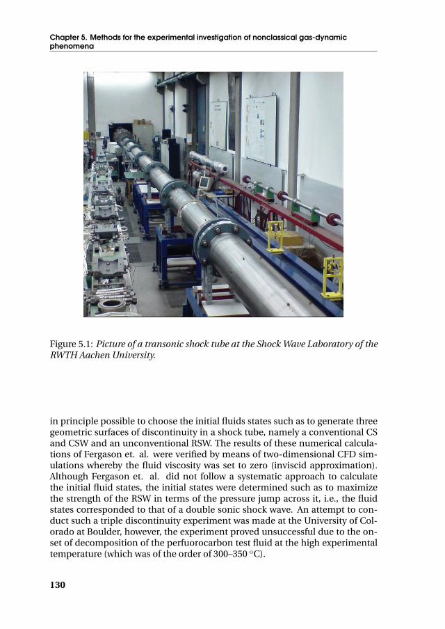
Chapter 5. Methods for the experimental investigation of nonclassical gas-dynamicphenomena
Figure 5.1: Picture of a transonic shock tube at the Shock Wave Laboratory of theRWTH Aachen University.
in principle possible to choose the initial fluids states such as to generate threegeometric surfaces of discontinuity in a shock tube, namely a conventional CSand CSW and an unconventional RSW. The results of these numerical calcula-tions of Fergason et. al. were verified by means of two-dimensional CFD sim-ulations whereby the fluid viscosity was set to zero (inviscid approximation).Although Fergason et. al. did not follow a systematic approach to calculatethe initial fluid states, the initial states were determined such as to maximizethe strength of the RSW in terms of the pressure jump across it, i.e., the fluidstates corresponded to that of a double sonic shock wave. An attempt to con-duct such a triple discontinuity experiment was made at the University of Col-orado at Boulder, however, the experiment proved unsuccessful due to the on-set of decomposition of the perfuorocarbon test fluid at the high experimentaltemperature (which was of the order of 300–350 oC).
130

5.2 Unsteady experiments
P4
x
P3 P2
P1
P t
4
4 3 2 1
1
4 1
P4
P3 P2
P1
P t
x
RF CS CSW
RSW CS CSW
3 2
Figure 5.2: Upper: sketch of P -x- and t-x-diagrams of a conventional shock tubefeaturing classical wave fields: here, a left-moving RF, a right-moving CS and aright-moving CSW are observed. Lower: sketch of P -x- and t-x-diagrams of ashock tube featuring nonclassical wave fields: here, a left-moving RSW, a right-moving CS and a right-moving CSW are observed. Adapted from Ref. [64]
131

Chapter 5. Methods for the experimental investigation of nonclassical gas-dynamicphenomena
5.2.1.2 Initial fluid-states for a triple-discontinuity experiment
The initial states for a triple-discontinuity experiment can be chosen in order toeither maximize the pressure jump across the RSW, i.e., via a unique double-sonic expansion shock wave, or to maximize the supersonic-to-sonic transi-tion through the unsteady wave, which is an original idea that was proposedduring the first year of this research project. An experiment maximizing thepressure jump across the discontinuity was proposed by Fergason et. al. [64].The RSW was to be identified by observing an abrupt pressure decrease as thewave passed the dynamic pressure instruments which are flush-mounted onthe pipe wall of the high-pressure compartment, and its speed-of-propagationwas to be measured using a time-of-flight technique. Yet, in the case of a dou-ble sonic RSW, it may be potentially difficult to unambiguously assert from theresults of a measurement of the pressure drop and the wave speed, whetheror not the observed expansive wave is a nonclassical expansion shock waveor a classical expansion fan. This is a point of concern primarily because adouble sonic shock wave moves at sonic speed with respect to a shock-relatedframe of reference, just as the front runner wave of an expansion fan. Sec-ondly, expansion shock waves necessarily feature a rather small jump in pres-sure, namely O ([P ]) = 1 bar, and, due to i) a low value of Γ which can be ofthe order of 0.1, ii) the influence of thermoviscous effects, and iii) thermal relax-ation effects (since BZT fluids are necessarily molecularly complex), the shockthickness can be significant. In air for example under ideal-gas conditions, theshock-wave thickness for a shock-Mach number of about unity, is of the orderof 0.1 µm. However, in D6 in the dense-gas regime, the thickness of a nonclas-sical RSW can be of the order 1–10 µm depending on the ratio of the bulk vis-cosity with respect to the shear (dynamic) viscosity, which can be in the rangeO (ζ/η) = 1− 102 [62] (see also Chap. 6, Table 6.1). It is also known from experi-ments with carbon dioxide, for example, that weak shock waves can be fully dis-persed and therefore rather thick (refer to Fig. 232 on pg. 140 of Van Dyke [208]showing an 8-mm thick shock wave in CO2 with a shock Mach number of 1.04;the dispersed structure is due to slow vibrational relaxation). Consequently, thedynamic-pressure instruments may not detect a rather sharp decrease of pres-sure in time as one might have anticipated based on measurements/experienceof/with weak shock waves in air. Additional complications can arise if the ex-pansion wave features shock-fan composite behavior, or if the dynamic pres-sure instruments (which have a finite response time) are not well synchronized,and/or if crude noise-filtering is used, thereby potentially being the cause of amisinterpretation of the measurements.
The arguments presented in the previous paragraph against an experimentfeaturing a double-sonic RSW however, do not rule-out the effectiveness of per-forming a triple-discontinuity experiment in a shock tube. In fact, an experi-ment using a time-of-flight method whereby an expansion shock wave whichdisplays the highest supersonic-to-sonic transition, may be used to unequivo-
132

5.2 Unsteady experiments
cally demonstrate nonclassical RSW’s. Here, a unique interpretation of the ex-perimental pressure signals is possible. Due to the fact that only shock waves,independent of their nature, propagate at supersonic speed,1 whereas the frontrunner wave of fans move at sonic speed, nonclassical RSW’s displaying thehighest supersonic-to-sonic transition, move the fastest with respect to the stillfluid. Therefore, a time-of-flight method can be used to determine the wavespeed and the wave-Mach number; if and only if the obtained wave Mach num-ber, taking the uncertainties into account, is greater than unity can it be claimedthat the expansive wave is a nonclassical RSW.
With reference to Fig. 5.2, the initial states (P1, v1, u1 = 0) and (P4, v4, u4 = 0)that admit three discontinuities in a conventional shock tube with the samefluid as driver and driven gas, can be determined as indicated in the following.The delineated procedure is valid if: i) the entire tube is maintained at a con-stant temperature, i.e., T1 = T4, ii) the fluid is inviscid, iii) the waves are planar,iv) the flow is nearly one-dimensional, v) the geometric surfaces of discontinu-ity are instantaneously formed (meaning that if a diaphragm is employed, theopening time is effectively zero), and vi) the flow is rotation free.
1. Since a time-of-flight method is to be used, the aim is to create an RSWwhich features a transition from state 4 to 3 with a post-shock Mach num-ber of unity whereby the pre-shock Mach number, Ma4, is maximized. Fordodecamethylcyclohexasiloxane (D6) as the test fluid or alternatively fortetradecamethylhexasiloxane (MD4M), it follows from the Ma-v-plot de-picted in Figs. 2.9 and 5.3 respectively, that the thermodynamic proper-ties of state 4 correspond to saturated-vapor conditions, namely to that ofpoint O.
2. The properties of post-shock state 3 are located on line M-N in Figs. 2.8and 5.5 for fluids D6 and MD4M, respectively. The values of v3, P3 and u3
are determined iteratively from
h3 (P3, v3) = h4 +12
(P3 − P4) (v3 + v4) , (5.1a)
JRSW ≡w3
v3=w4
v4=
√−(P3 − P4
v3 − v4
), (5.1b)
u3 = w3 −w4, (5.1c)
taking into account that
Ma3 ≡w3
c3= 1, (5.2a)
Ma4 ≡w4
c4> 1, (5.2b)
[s] = s3 − s4 ≥ 0. (5.2c)1double-sonic and RSW’s with a pre-shock Mach number of unity are an exception.
133

Chapter 5. Methods for the experimental investigation of nonclassical gas-dynamicphenomena
vV [m3/kg]
Ma
[-]
ΓV[-
]
[P]
[bar
]
0.004 0.005 0.006 0.007 0.008 0.0091.00
1.01
1.02
1.03
1.04
-0.4
0.0
0.4
0.8
-1.6
-1.2
-0.8
-0.4
0.0OPRSV
OSW MPRSVMSWDSWDPRSV
Figure 5.3: The pre-shock Mach number (solid lines) – whereby the post-shockMach number is equal to unity – as a function of the saturated vapor specificvolume (vV) of MD4M. Thermodynamic properties are determined with the EoSdocumented in Ref. [33] (black lines) and the PRSV EoS (red lines). The dashedlines give the pressure jump [P ] across the RSW and the dash-dotted lines repre-sent the value of Γ in the pre-shock state. The points labeled “D” indicate shockstates with a pre- and post-shock Mach number of one, the points labeled “M”represent the limiting RSW’s with [P ] = 0, and points “O” give the pre-shock statewith the greatest supersonic-to-sonic speed change.
The equality sign for the entropy jump is only valid for infinitely weakshock waves satisfying [s] ↓ 0.
3. The results obtained from the shock admissibility conditions when ap-plied to the RSW, facilitate the computation of the properties behind andahead of the CSW, i.e., states 2 and 1 respectively, by considering that: i)the change of velocity across a CS is purely tangential, i.e., there is no massflow through an ideal CS, and ii) that for an inviscid fluid, the pressures on
134

5.2 Unsteady experiments
both sides of the CS are equal, namely
u2 = u3, (5.3a)
P2 = P3. (5.3b)
4. Using an iterative scheme, the properties of state 1 are obtained from
h2 (P2, v2) = h1 +12
(P2 − P1) (v1 + v2) (5.4a)
JCSW ≡w1
v1=w2
v2=
√−(P2 − P1
v2 − v1
)(5.4b)
u2 = w2 −w1 (5.4c)
as follows:
- Guess the value of P1 < P2 and determine v1 using the EoS of theworking fluid and the fact that T1 = T4 is imposed.
- Using the equation for the shock adiabat through state 1, compute v2.
- Using the Rayleigh equation, calculate w1, w2 and u2.
- Check that Ma2 ≡w2
c2< 1, Ma1 ≡
w1
c1> 1, and s2 − s1 > 0.
- If the new value of u2 differs significantly from the value obtained viathe shock admissibility conditions applied to the RSW, make a newguess for P1 and iterate until convergence is obtained.
The described successive steps are applied to BZT fluid MD4M [30] wherebythermodynamic properties are computed with the Peng-Robinson, Stryjek andVera modified, cubic (PRSV) EoS using the fixed fluid parameters documentedin Table 3.15. The PRSV EoS was selected for the calculations because, as wasindicated in Sec. 4.6, model EoS’s, although less accurate than multiparame-ter EoS’s, do correctly account for the thermodynamic and physical behavior ofthe fluid with the least number of parameters possible. This is important if athermodynamic model is applied to a fluid for which only a limited number ofexperimental data are available.
The initial states 1 and 4 of the triple-discontinuity experiment and the prop-erties of the intermediate states 2 and 3 are listed in Table 5.1. These values areconfirmed with one-dimensional CFD simulations of the triple-discontinuityexperiment using version 1.00 of the software zFlow [36], a CFD solver usingreal-gas properties. The computational grid contains 400 cells with a node-spacing of x/L = 0.0025, the time integration is done with a 2nd-order Runge-Kutta scheme and the CFL number is 0.5. Furthermore, it is assumed that thediaphragm ruptures instantaneously. Results of these computations are dis-played in Fig. 5.4. An important note is that these calculations were performed
135

Chapter 5. Methods for the experimental investigation of nonclassical gas-dynamicphenomena
L [m]
P[b
ar]
Γ[-
]
ρ[k
g/m
3 ]
-5 -2.5 0 2.5 55.5
6.0
6.5
7.0
7.5
8.0
8.5
9.0
-0.2
0.0
0.2
0.4
0.6
60
80
100
120
140
160
180
200
t = 46.1 ms
P[b
ar]
Γ[-
]
ρ[k
g/m
3 ]
5.5
6.0
6.5
7.0
7.5
8.0
8.5
9.0
-0.2
0.0
0.2
0.4
0.6
60
80
100
120
140
160
180
200
t = 26.3 ms
Figure 5.4: zFlow simulation of the triple-discontinuity experiment in a conven-tional shock tube using BZT fluid MD4M. Thermodynamic properties are calcu-lated with the Peng-Robinson EoS with the Stryjek and Vera modification. Thesolid line represents the pressure profile and the dashed and dash-dotted linesrepresent the Γ- and density profile, respectively.
136

5.2 Unsteady experiments
Table 5.1: States 1–4 according to Fig. 5.2 of a triple discontinuity experimentconducted with MD4M as working fluid. Thermodynamic properties are cal-culated in the PRSV EoS. A positive (negative) velocity indicates fluid flow to-wards the right (left) with respect to the laboratory frame of reference. Note[P ] = 121.1 kPa.
State P [kPa] ρ [kg/m3] T [oC] u [m/s] w [m/s] c [m/s] |Ma| [–]
1 602.9 75.57 377.2 0 -77.58 77.82 1.080
2 720.7 102.0 380.2 +20.09 -57.50 61.76 0.9310
3 720.7 113.2 371.4 +20.09 +53.27 53.27 1.000
4 841.8 181.8 377.2 0 +33.19 31.94 1.039
in 2005 employing the older ThermoProp fluid properties library, therefore theflow properties reported in Table 5.1 are slightly different than the values dis-played in the respective figures, however, qualitatively, the flow features are un-changed.
5.2.1.3 Influence of secondary effects on shock-tube experiments
The following items, although some are mostly based on experimental and nu-merical studies of classical flows of simple fluids (see references herein), theseare qualitatively applicable also to nonclassical flows of dense gases. From aquantitative viewpoint, it is still an unanswered question whether or not ac-counting for these secondary effects, even yields numerically correct results,particularly because of the lack of experiments conducted with molecularly com-plex dense gases.
In the determination of the initial states of a triple-discontinuity experimentin a shock tube, it was assumed that the discontinuities are planar, the flow isquasi one-dimensional and that the flow past the discontinuities is a potentialflow. In the case of BZT fluids however, the following aspects must be accountedfor and the validity of the assumptions must be assessed (see Chap. 6 where thebelow-mentioned aspects have been considered during the preliminary designof the test facility).
137

Cha
pte
r5.M
etho
ds
forthe
expe
rime
ntalinve
stiga
tion
ofno
nclassic
alg
as-d
ynam
icp
heno
me
na
v [m3/kg]
P[k
Pa]
0.002 0.004 0.006 0.008 0.010650
700
750
800
850
900
N
M
O
D
Vapor-liquidEquilibrium Region
Γ = 0 - line
Post-shock statesfor pre-shock stateslocated on the dew-line
Tm
ax =400
oC
(a) Results from the PRSV EoS
v [m3/kg]
P[k
Pa]
0.002 0.004 0.006 0.008 0.010650
700
750
800
850
900
N
M
O
D
Vapor-liquidEquilibrium Region
Γ = 0 - line
Post-shock statesfor pre-shock stateslocated on the dew-line
Tm
ax =400
oC
(b) Results from the multiparameter EoS of Ref. [33]
Figure 5.5: The Γ < 0-region of MD4M in the P -v-plane calculated with two EoS’s. The dotted line indicates post-shockstates with a Mach number of one, point O represents the thermodynamic state on the dew-line that displays the greatestsupersonic-to-sonic transition and point D gives the thermodynamic state on the dew-line which features both a pre-and post-shock Mach number of unity (the sonic post-shock state of point D is point N). Point M is the limiting case ofan RSW with [P ] = 0.
138

5.2 Unsteady experiments
- Incomplete rupture of the diaphragm:In the case that a diaphragm is used in the shock tube, complications mayarise due to its incomplete rupture. See for example the experimental andnumerical study conducted by Gaetani et. al. [75] where results showthat the shock intensity is lower in the case of incomplete diaphragm rup-ture compared to when the diaphragm ruptures completely, and multi-dimensional disturbances are generated due to shock diffraction from thediaphragm edges and results in a complex unsteady flow field behind theleading shock wave. The numerical study by Gaetani et. al. was done em-ploying an unsteady Euler solver documented in Ref. [83] and assumingnegligible viscosity, thermal conductivity, and a polytropic ideal gas. Alsorefer to Fergason’s PhD thesis [65] where pictures are included, namelyFig. 7.6 therein, showing incomplete rupture of a scorched metallic di-aphragm; the test fluid was nitrogen gas at 350 oC and a low pressuredifference, i.e., between 0.6–0.7 atm. similar to that of the foreseen ex-periment with the provisional working fluid, was used to rupture the di-aphragm. Moreover, the experimenter has little control over the momentof rupture and the opening time, especially because the experiments haveto be conducted at elevated temperatures (300-400 oC). Also, because ofthe high temperatures involved and purity requirements of the test fluid,the availability of the shock tube equipped with a diaphragm is low. Fi-nally, it must be indicated that due to the fact that the moment at whichand the manner that the diaphragm breaks are difficult to control, the re-peatability and the reproducibility of the experiments is poor.
- The effect of the boundary layer:The boundary layer which is formed behind the shock wave results ina loss of homogeneity of the flow. Consequently, a non-negligible por-tion of the mass contained in the plug, i.e., the region between the shockwave and the CS, gets accumulated in the boundary layer and intermixingof the driver and driven gas takes place through the CS which becomesnon-planar [193]. Additionally, weakening of the pressure jump across theshock wave and the shock speed take place during propagation.
There are numerous investigations devoted to the numerical and experi-mental study of boundary layers in shock tubes. Notable studies are thatof Donaldson and Sullivan [55], Hollyer [94], Mirels [144, 145], and Trimpiand Cohen [204]. Donaldson and Sullivan for example, determined thedeceleration of a shock wave due to the formation of an incompressibleboundary layer, therefore, their model is only valid for weak shock waves,e.g., nonclassical RSW’s. Trimpi and Cohen [204] on the other hand reducethe problem to a one-dimensional flow and apply a correction to the in-compressibility assumption of the boundary layer. They provide an equa-tion for determining the attenuation across the shock wave in terms of thepressure jump. Interestingly enough, if linear attenuation is accounted for,
139

Chapter 5. Methods for the experimental investigation of nonclassical gas-dynamicphenomena
it was found that for a specific range of shock pressure ratios, strength-ening of the wave occurred and that the larger the shock-tube Reynoldsnumber, i.e., ReD = u2D/ν2, whereD is the shock tube diameter, the lowerthe pressure jump attenuation. Experimental studies on classical flows ofsimple fluids have shown that for shock waves with a shock-Mach numberless than 4, the transition from a laminar to a turbulent boundary layer oc-curs at Reynolds numbers Rex of 2 · 105 (see Refs. [87, 88]) – 3 · 106 (see Ref.[138]), where the lower limit was found in shock tubes with rough walls.2
- The effect of the uncertainty in the prediction of thermodynamic prop-erties:The thermodynamic description of the fluid significantly influences thequalitative and quantitative prediction of the flow features and flow vari-ables. In this respect the sensitivity of the results due to the uncertaintyin the ideal-gas isobaric heat capacity prediction, which can be quanti-fied (see Sec. 3.2), is investigated. Although P -v-T -properties are left un-influenced by the uncertainty in the predicted values of C0
P , the caloricproperties do change. As a consequence of the uncertainty in C0
P valuesof 5 % for siloxanes, if the same pressure and temperature listed in Ta-ble 5.1 are used for states 1 and 4 of a triple-discontinuity experiment, thefollowing can occur: i) either the rarefaction shock wave splits into a com-posite shock-fan; in this case the post-shock Mach number is still unity,on the other hand the pressure jump can be less than the 121.1 kPa com-puted using the values listed in Table 5.1, or ii) the rarefaction shock wavedoes not feature a supersonic-to-sonic transition, but rather a supersonic-to-subsonic transition. In the most extreme situation, e.g., if C0
P valuesare significantly overpredicted, it is also possible that the rarefaction wavedoes not steepen into a shock front but evolves as an isentropic rarefactionfan instead. The results of an exemplary calculation for MD4M taking the5 % uncertainty inC0
P predictions into account, are presented in Tables 5.2and 5.3 where the PRSV EoS is used. Figures 5.6 and 5.7 display the sensi-tivity of the results given in Fig. 5.3 to the uncertainty inC0
P . As a remark itshould be mentioned that the quantitative prediction of the flow featuresand flow variables are also sensitive to the uncertainty in thermal propertydata, however, only the uncertainty in C0
P can be rigourously justified (seealso the concluding remarks of Chap. 4).
- The influence of non-equilibrium effects:Non-equilibrium effects cause the density and temperature profile behindthe discontinuities to be non-negligibly different than their equilibriumcounterparts. The pressure profile however is only slightly affected, al-though this is only confirmed for substances composed of rather simple
2In this context, Rex = xρ2(w2
2
)/ (η2u2), and x is the distance from the shock front [193]. Note
that Trimpi and Cohen [204] define Rex = xρ2u2/η2.
140

5.2 Unsteady experiments
vV [m3/kg]
Ma
[-]
ΓV[-
]
[P]
[bar
]0.004 0.005 0.006 0.007 0.008 0.009
1.00
1.01
1.02
1.03
1.04
1.05
1.06
-0.4
0.0
0.4
0.8
-2.0
-1.6
-1.2
-0.8
-0.4
0.0
O
O’’
O’O’
Figure 5.6: Sensitivity of the results displayed in Fig. 5.3 for MD4M to the 5 % un-certainty in the isobaric-heat-capacity prediction, see Sec. 3.2. Note that only thePRSV EoS is considered; these results are qualitatively similar to those obtainedwith the SW EoS. Legend: the red lines are the result of an over-predicted value forC0P , whereas the blue lines are the result of an under-predicted value for C0
P . Thereference C0
P values are determined with Eq. (3.18) using the parameters listedin Table. 3.13. The solid lines represent the pre-shock Mach number, the dashedlines give the pressure drop over the predicted rarefaction shock wave and thedash-dotted lines give the value of Γ along the dew-line for relevant pre-shockstates. Points O, O’ and O” represent the maxima in the pre-shock Mach numberfor admissible RSW’s.
141

Chapter 5. Methods for the experimental investigation of nonclassical gas-dynamicphenomena
v [m3/kg]
P[k
Pa]
0.004 0.005 0.006 0.007 0.008 0.009 0.010650
700
750
800
850
900
N
M
O
D
Vapor-liquidEquilibrium Region
Tm
ax =400 oC
TC
O’O’’
D’D’’
M’’
M’
N’’
N’
Figure 5.7: Sensitivity of the size of the Γ < 0-region of MD4M due to the 5 % un-certainty in the isobaric-heat-capacity prediction, see Sec. 3.2. Only the PRSV EoSis considered. Legend: the red lines are the result of an over-predicted value forC0P , whereas the blue lines are the result of an under-predicted value for C0
P . Thereference C0
P values are determined with Eq. (3.18) using the parameters listedin Table. 3.13. The solid line delimits the vapor-liquid equilibrium region, thedashed lines give the Γ = 0-line in the superheated vapor region, the dotted linesindicate the post-shock states featuring a Mach number of unity, whereby the pre-shock Mach number is maximized; moreover, pre-shock states are located on thedew-line, and the dash-dotted lines indicate isotherms. Points O, O’ and O” rep-resent the maxima in the pre-shock Mach number for admissible RSW’s, as iden-tified in Fig. 5.6, points D, D’ and D” represent the pre-shock states with a Machnumber of one (the associated post-shock states are indicated by points N, N’ andN”, respectively), and points M, M’ and M” represent limiting sonic RSW’s witha pressure jump of zero. Note the discontinuity in the slope of the Γ = 0-line atT = TC due to the inconsistency of the PRSV EoS.
142

5.2 Unsteady experiments
Table 5.2: Properties 1–4 of the triple-discontinuity experiment whereby thepressure and temperature of states 1 and 4 are the same as the values listedin Table 5.1, however increasing the C0
P prediction by 5 %. Note that the RSWfeatures a pressure jump of 121 kPa.
State P [kPa] ρ [kg/m3] T [oC] u [m/s] w [m/s] c [m/s] |Ma| [–]
1 602.9 75.57 377.2 0 -77.38 71.72 1.079
2 720.8 102.2 380.0 +20.16 -57.22 61.43 0.9316
3 720.8 112.9 371.7 +20.16 +53.19 53.36 0.997
4 841.8 181.8 377.2 0 +33.04 31.49 1.049
Table 5.3: Properties 1–4 of the triple-discontinuity experiment whereby thepressure and temperature of states 1 and 4 are the same as the values listedin Table 5.1, however decreasing the C0
P prediction by 5 %. Note that the RSWfeatures a pressure jump of 114.4 kPa. The RSW is immediately followed by ararefaction fan featuring transition 3–3’.
State P [kPa] ρ [kg/m3] T [oC] u [m/s] w [m/s] c [m/s] |Ma| [–]
1 602.9 75.57 377.2 0 -77.47 71.92 1.077
2 714.6 100.3 380.1 +19.08 -58.39 62.58 0.9330
3’ 714.6 111.6 370.9 +19.08 N.A 53.96 N.A.3 727.4 116.1 371.4 +18.87 +52.23 52.23 1.000
4 841.8 181.8 377.2 0 +33.36 32.43 1.029
molecules like Ar and O2 [192]. This means that because the time-of-flight method uses pressure instruments to detect when the leading wavereaches the sensors, non-equilibrium effects will probably not be detected.However, the flow field itself can be radically different than what followsfrom equilibrium relations depending on the severity of the departure fromequilibrium. In the case of polyatomic gases, such as BZT fluids, vibra-tional relaxation is the main point of concern, since contrary to transla-tional and rotational equilibrium, which is achieved in only few collisions,the achievement of vibrational equilibrium may require thousands of col-lisions [121]. Moreover, polyatomic gases have several modes of molec-ular vibration – each of which can, in principle, relax independently –and are structurally flexible. Consequently they can change their shape,both during normal vibration and during collision, the latter being prob-ably more relevant. The majority of polyatomic gases exhibit a single vi-brational relaxation process, which involves the entire vibrational energycontent of the molecule. This is based on the assumption that vibrational-vibrational energy transfer is faster than vibrational-translational energy
143

Chapter 5. Methods for the experimental investigation of nonclassical gas-dynamicphenomena
transfer, therefore the total vibrational energy content of a molecule re-laxes by vibrational-translational energy transfer via the lowest mode. Forestimating the time for vibrational relaxation, the mode of the lowest fre-quency of vibration is required. These data were determined from ab ini-tio calculations, as treated by Nannan et. al. [153]. The computed lowestfrequency of vibration for all the siloxanes considered in Chap. 3 (this in-cludes D6) is lower than 40 cm−1 (data provided by Prof. Richard Rowleyof BYU, UT). By using the Lambert-Salter plot, documented in Chap. 3,pg. 64 of Ref. [121], for molecules containing more than two hydrogenatoms, the vibrational relaxation time is estimated to be of the order of 0.1nanoseconds, i.e., 10−10 sec at 300 K. The fact that the pre- and post shockstates for rarefaction shock waves are at a higher pressure and tempera-ture, should not have a significant effect on the estimation of the order ofmagnitude of the vibrational relaxation time [121]. As in Ref. [201], therarefaction shock thickness for D6 can be computed based on: i) the cal-culated viscosity using the method of Chung et. al., ii) the assumption thatthe bulk viscosity is of the same order of magnitude as the shear viscosity,and iii) that the ratio of the isobaric with respect to the isochoric heat ca-pacity is of the order of 1. This results in an estimated shock thickness ofthe order of micrometers and therefore the residence time of the molecule– for a speed of sound of about 40 m/s – is of the order of 10−8 sec. Accord-ing to these calculations, the relaxation time is at least two orders of mag-nitude smaller than the residence time of a molecule in the shock. Equi-librium of the internal energy can therefore be assumed past the shockwave.
5.2.2 Point explosions in dense gases
Sufficiently far from the source of a disturbance, as for example are the pres-sure waves caused by supersonic aircrafts or resulting from explosions, spher-ical waves are perceived as weak N-waves, so-named due to the shape of thepressure profile as a function of the distance from the center of origin [178].Under laboratory conditions, N-waves are created in simple spherical cavitiesoften containing air, by using sparks, exploding wires, or a pulsed laser.
The possibility of using point explosions and thus the resulting N-waves asa means to provide experimental proof for the existence of nonclassical wavefields, particularly nonclassical compression waves, is numerically investigatedand discussed by Guardone and Colonna [82]. This idea of employing point ex-plosions to study phenomena associated with nonclassical gas dynamics wasinitiated based on earlier tests conducted at the University of Maryland by Dr. F.Ferioli [67] related to Laser-Induced Breakdown Spectroscopy (LIBS) measure-ments in hydrocarbons.3 In the experimental facility at the University of Mary-
3LIBS can be used for quick gas composition measurements.
144

5.2 Unsteady experiments
land, a focusing pulsed laser was used to create a hot plasma expanding in aninitially still, cold gas confined in a spherical cavity.
In the classical case, e.g., if diatomic nitrogen is used as test medium, andif dissociation and ionization do not occur due to the localized energy input,concentration of a fixed amount of thermal energy at the center of the sphericalcavity results in the formation of classical N-waves. In fact, the localized releaseof energy results in the formation of a succession of compression and rarefac-tion waves. The compression waves steepen into a shock wave and move fur-ther from the point of origin, whereas the rarefaction waves move towards thecenter. As the distance between the leading compression shock wave and thecenter increases, the amplitude of the pressure profile of the CSW attenuatesand the wave speed gradually decreases (the observed attenuation and disper-sion depend on the magnitude of the energy input). Furthermore, the focussingrarefaction waves eventually admit a second compression shock wave whichpropagates away from the center. In between the initial CSW and the RF, a CS ispresent.
Due to the difficulty of the prediction of the formation of N-waves fromsparks or exploding wires and the additional complications caused by relax-ation phenomena, often the theoretical study of point explosions is conductedby means of numerical simulation whereby the energy input/explosion is ap-propriately modeled. In Ref. [95] for example, the formation of an N-wave dueto a localized explosion in air is studied assuming a pressurized sphere of smallradius at room temperature separated from the outside air by an imaginarydiaphragm, see Fig. 5.8. Initially, the temperature is uniform and the abso-lute fluid velocities are zero. The simulation starts by removing the diaphragmand solving the fully compressible Navier-Stokes governing equations assum-ing spherical symmetry and constant-valued transport properties. Moreover,energy transfer related to relaxation phenomena can be taken into account inthe governing equations.
A similar approach utilizing an imaginary diaphragm is used by Guardoneand Colonna [82] in their study of nonclassical N-waves in fluid D6. Contrary tothe procedure adopted by Honma and Glass documented in Ref. [95] wherebythe initial temperature is the same on both sides of the imaginary spherical di-aphragm, Guardone and Colonna assume the density of the fluid contained inthe inner sphere to be equal to that contained in the outer sphere. Furthermore,relaxation phenomena are not modeled, thermoviscous effects are not consid-ered, however, real-gas behavior is accounted for by employing the Martin-HouEoS to D6. Moreover, the initial pressure and density on the low-pressure side(i.e., the fluid contained in the outer sphere) is slightly supercritical whereasthe initial thermodynamic state on the high-pressure side of the imaginary di-aphragm is located inside the negative nonlinearity region (Γ < 0-region). Ad-
145

Chapter 5. Methods for the experimental investigation of nonclassical gas-dynamicphenomena
ditionally, the fluid velocity is zero everywhere. In brief,
ρ (r)ρC
= 0.47169 ∀ r
u (r) = 0 m/s ∀ rP (r)PC
={
0.8700 if Ri < r ≤ Ro
1.200 if 0 ≤ r ≤ Ri,
(5.5)
where inner radius Ri = 1 mm and the inner radius of the outer sphere Ro =150 mm. The critical density and pressure adopted by Guardone and Colonnawere respectively, 276 kg/m3 and 9.6 bar.
The results of the simulation with D6 show that indeed the compressionwave spreads out in time as an isentropic compression fan. The rarefactionwave on the other hand does not coalesce into an expansion shock wave. Addi-tionally, numerically simulated Schlieren images of the point explosion demon-strate that the use of an optical arrangement does not allow for a detection ofthe compression fan. Therefore, the spreading of the compression fan has tobe measured by using total pressure probes positioned at various distances, sayR1 and R2, from the center of origin. Provided that the probes themselves donot influence the flow field – although this must be investigated in more detail,e.g., by using CFD analysis – a nonclassical wave yields forR2 > R1 ⇒∆t (R2) >∆t (R1), where ∆t = t′ − t′′, and t′ and t′′ being the times at which the compres-sion profile starts and ends, respectively.
5.3 Steady experiments
Steady experiments are classified as those having a steady flow field and wherethe nonclassical gas-dynamic phenomenon under scrutiny remains steady withrespect to a laboratory reference frame. Two steady experiments can be envis-aged for studying flow phenomena which are the result of Γ being (locally) lessthan zero, namely: i) an experiment which creates a steady nonclassical rarefac-tion shock wave or a series of both nonclassical and classical shock waves whichare typical only of BZT fluids in a classical converging-diverging nozzle, or ii) anexperiment whereby a nonclassical two-dimensional wave field is created dueto turning of a supersonic flow over a body. Both of these options are discussedin the following.
5.3.1 Nonclassical shock waves in a classical nozzle
5.3.1.1 Overview – steady isentropic flows of BZT fluids in one dimension
A numerical investigation into the occurrence of shock waves, be it classicalor nonclassical, in steady, inviscid flows of a BZT fluid in classical converging-
146

5.3 Steady experiments
Spherical cavity
Point explosion
Imaginary diaphragm
P
r r
P
Ri
T T
E0
Figure 5.8: Top left: point explosion occurring in the center of the spherical cav-ity releasing a concentrated amount of energy E0. Bottom left: the pressure andtemperature as a function of the radial coordinate at t = 0. Top right: Modelof the point explosion. Here, an imaginary diaphragm separates the high- andlow-pressure sides. The diaphragm instantaneously disappears at t = 0. Bottomright: the pressure and temperature as a function of the radial coordinate at t = 0where Ri is the radius of the inner spherical cavity.
147

Chapter 5. Methods for the experimental investigation of nonclassical gas-dynamicphenomena
diverging nozzles is documented by Cramer and Fry [41]. Their study is an ex-tension of earlier works of Chandrasekar and Prasad [24] and Kluwick [112].
Consider a classical converging-diverging nozzle. From a control-volumeperspective, if the flow is one-dimensional, inviscid, single-phase, isentropic,steady and free of body forces, then the governing equations are (subscript “0”indicates stagnation (total) properties)
m = ρuA = constant
h0 = h+u2
2= constant
s0 = s = constant
(5.6)
Using the differential form of Eqns. (5.6), namely
1A
dA
dx+
1u
du
dx+
1ρ
dρ
dx= 0 (5.7a)
dh
dx+ u
du
dx= 0 (5.7b)
ds
dx= 0 (5.7c)
and the fact that Tds = dh − dP/ρ = 0, Ma = u/c, dP = c2dρ, and dc =c (Γ− 1) dρ/ρ because of Eq. (5.7c), it can be demonstrated with Eq. (5.7b) that[196]
dMadρ
=Maρ
(1− Γ− 1
Ma2
)︸ ︷︷ ︸
℘
. (5.8)
Or, by using the differential form of the mass conservation equation, namelyEq. (5.7a), it is found that
1Ma
dMadx
=1 + (Γ− 1) Ma2(
Ma2 − 1) 1
A
dA
dx, (5.9)
and
1ρ
dρ
dx=(
Ma2
1−Ma2
)1A
dA
dx. (5.10)
Starting from a specific stagnation state on an isentrope, Figs. 5.9 and 5.10illustrate the local Mach number computed using Eq. (5.8), with respect to thereduced density of fluid D6. Thermodynamic properties are obtained with thePRSV EoS. As demonstrated by Cramer and Best [47], the results presented inthese figures show that, depending on the choice of the stagnation conditions,steady isentropic expansion of a BZT fluid in the dense-gas regime to super-sonic conditions results in the occurrence of at least one, and at most three
148

5.3 Steady experiments
sonic points. What is more is that passage of the first sonic point is necessarily astate with Γ > 0. All of the stagnation states for which the trend lines are drawnin Fig. 5.9 for example, exhibit only one sonic point. Figure 5.10 shows the Ma-ρ-plot for two stagnation states selected along the isentrope which is tangentialalong to the VLE region on the dew-line of D6 (s = sV
max), which exhibit threesonic points. As a last remark, it is observed that in Fig. 5.9 the dashed line, i.e.,the line connecting states with ℘ = 0 as defined in Eq. (5.8), intersects the sonic(Ma = 1) line twice. This only occurs if the isentrope along which the fluid is ex-panded from stagnation to supersonic conditions exhibits Γmin < 0. Isentropeswith 0 < Γmin < 1 display a qualitatively similar trend as shown in Fig. 5.9,however for these isentropes, the ℘ = 0-line is located completely above thesonic line, since Mamin, ℘=0 = (1− Γmin)−1/2
> 1, see Ref. [47]. Consequently,isentropes with 0 < Γmin < 1 feature, depending on the stagnation state, non-monotonous Ma-ρ-trend lines which can have two extremes; these extremesoccur at supersonic conditions and because of this, these isentropes only havea single sonic point. Finally, isentropes with Γmin > 1 display monotonous Ma-ρlines and admit a single sonic point in the case of steady isentropic expansionfrom stagnation to supersonic conditions, because ℘ < 0.
Utilizing the results displayed in Figs. 5.9 and 5.10, one can either compute,using Eqns. (5.9) and (5.10), for a given stagnation state on a specific isentrope,the area variation. Alternatively, which within the context of this chapter is moreinteresting, for a given area as a function of the spatial coordinate x, the localflow variables can be determined and the shock admissibility conditions can beused to identify steady shock waves.
5.3.1.2 Creating steady nonclassical shock waves in classical nozzles
Based on the fact that – and depending on the choice of the stagnation (reser-voir) conditions – steady, isentropic expansion of a BZT fluid can result in theoccurrence of at least one, and at most three sonic points (see Figs. 5.9 and5.10), three types of flow can be distinguished. Numerical calculations [41],confirmed by mathematical and physical reasoning and computations (see e.g.,Ref. [24, 112]), have shown the admissibility of two nonclassical types of flowwhich feature, among a variety of nonclassical gas dynamic discontinuities, rar-efaction shock waves, and one classical type featuring well-known compressionshock waves which can be generated downstream of the throat. All the stagna-tion states displayed in Fig. 5.9 for example, give rise to purely classical com-pression shock waves past the nozzle’s throat. This is also what theoreticallyoccurs for steady isentropic expansion of dense gases if 0 < Γmin < 1 every-where in the flow (that is in fluids which are molecularly complex, but whichdo not classify as BZT fluids). Stagnation states which admit three sonic points,such as illustrated in Fig. 5.10, theoretically permit the above-mentioned non-classical flows; Cramer and Fry [41] refer to these nonclassical flows as type Iand II flows. More specifically, according to Cramer and Fry, type I flows occur if
149

Chapter 5. Methods for the experimental investigation of nonclassical gas-dynamicphenomena
ρR [-]
Ma
[-]
Γ[-
]
0.0 0.5 1.0 1.5 2.00.0
0.5
1.0
1.5
2.0
2.5
-0.1
0.0
0.1
0.2s = 1.07 kJ/kg-K
s = sVmax
Sta
gnat
ion
stat
e,s 0
=1.
07kJ
/kg-
KT
R0
=0.
995
Figure 5.9: Ma-ρ-plot for fluid D6 assuming isentropic expansion from variousstagnation states (reservoir conditions) (ρ0 (T0) , s0, u0 = 0). The blue lines are re-sults for the isentrope which is tangential to the VLE region on the dew-line forvarious stagnation temperatures (TR0 ≡ T0/TC = 0.995, 1.00, . . . , 1.02), whereasthe black lines are results for an isentrope (s = 1.07 kJ/kg-K) which is completelylocated in the superheated dense-gas region for 7 different stagnation tempera-tures (TR0 = 0.995, 1.00, . . . , 1.025). The solid lines indicate the functional rela-tion between the local flow Mach number and the local reduced fluid density (i.e.,ρR ≡ ρ/ρC), the dashed lines, where ℘ = 0 [see Eq. 5.8], connect the extremes ofthe individual Ma-ρ-lines for the isentropes affiliated with them and the dash-dotted lines indicates the value of Γ (only for the range of densities where Γ ≤ 0)along the considered isentropes. Remark that the selected isentropes exhibit pos-itive and negative nonlinearity. Thermodynamic properties are computed withthe PRSV EoS.
the sonic points labeled ρI2 and ρI
3 in Fig. 5.10 are closer to each other than sonicpoints ρI
1 and ρI2, whereas type II flows are found if the sonic points labeled ρII
1
and ρII2 in Fig. 5.10 are closer to each other than sonic points ρII
2 and ρII3 .
First consider the type II flows. For a given area variation A (x), Eqns. (5.9)
150

5.3 Steady experiments
ρR [-]
Ma
[-]
0.2 0.4 0.6 0.8 1.00.9
1.0
1.1
TR0 = 1.0085(Type I flows)
TR0 = 1.0082(Type II flows)
ρ1Iρ2
Iρ3I
ρ1IIρ2
IIρ3II
Figure 5.10: Ma-ρ-plot for fluid D6 assuming expansion from two different stag-nation states (not shown) along the isentrope which is tangential to the VLE re-gion on the dew-line. Observe three sonic points for each line compared to onlyone along each Ma-ρ-trend line in Fig. 5.9. Thermodynamic properties are com-puted with the PRSV EoS.
and (5.10) are just ordinary differential equations as a function of the spatialcoordinate x. Thus, if the area variation corresponding to that of a classicalconverging-diverging nozzle is specified, then with appropriate boundary con-ditions, Eq. (5.10) for example, can be solved numerically. The results can beconveniently displayed in so-called phase-plane plots, which, depending onan integration constant which among other things, is related to the mass flowthrough the nozzle, represents the graphical solution of Eq. (5.10) under the va-lidity of an equation of state (EoS). With reference to Fig. 5.10, Fig. 5.11 gives anexample of a phase-plane plot representing (some of the) mathematical solu-tions of a one-dimensional, steady isentropic expansion through a converging-diverging nozzle whereby the Ma-ρ-trend line exhibits three sonic points suchthat the points labeled ρII
1 and ρII2 are closer to each other than ρII
2 and ρII3 . Also
illustrated are admissible, so-called type II, discontinuities. Details are to be
151

Chapter 5. Methods for the experimental investigation of nonclassical gas-dynamicphenomena
x/L [-]
Ma [-]
ρ R[-
]
C1
C1*
C2
C2*
D1*
D1B1
B1*
B2
B2*
B3
B3*
B
C
D Thr
oat(
Ma
=1)
Ma
vs.r
educ
edde
nsity
Figure 5.11: The phase-plane diagram that can be used to analyze the admissibil-ity of type II shock waves in a conventional converging-diverging nozzle. The flowis from left to right. Remark that all phase-plane lines are for a single isentrope(s = s∗) and the same stagnation state, although the mass flow is different be-tween the various lines. Note that it was implicitly assumed that the shock wavesare weak and therefore density jumps are nearly isentropic. Also sketched is theMa-ρ variation (black dashed line) in the case of steady expansion of the fluidalong s∗ from one specific stagnation condition.
presented in the subsequent paragraphs, following Cramer and Fry.Note that for each individually colored curve in Fig. 5.11 (three of which are
labeled B, C and D), the entrance conditions, the mass flow and the throat areafor a given entrance area are the same, however, the mentioned conditions aredifferent among the differently colored curves. For a single curve, the main dif-ference in the actual physical flow is the entropy and pressure at the exit of thenozzle. Consider firstly curve B (green curve) in Fig. 5.11 representing the so-lution of an isentropic flow from left to right starting from subsonic conditions.As the fluid passes through the convergent section of the nozzle, the flow is ac-celerated from subsonic to sonic velocity in the throat. From the sonic throat
152

5.3 Steady experiments
onward (and assuming that the shock waves are weak), the following can occur:
- The flow expands to a supersonic speed and at a certain location, a non-classical RSW is admissible (labeled B1–B∗1). A discontinuity such as B1–B∗1 can also occur in the nozzle’s throat. Past the RSW, the flow is spedup further to finally give rise to the formation of a nonclassical sonic-to-subsonic CSW which exhibits the maximum strength in terms of pressurejump (labeled B3–B∗3). Past the CSW, the flow expands further but remainssubsonic.
- The flow expands to supersonic speed and eventually, a normal classicalCSW is admissible (labeled B2–B∗2). Also here, the flow expands furtherdownstream of the CSW but remains subsonic.
- The flow expands to supersonic speed, then it slows down to sonic speed,and eventually, a nonclassical upstream sonic CSW is permissible (labeledB3–B∗3).
Next, consider the curve labeled C, which is a solution if the mass flow isincreased somewhat or if the throat-area-inlet-area ratio AT/Ainlet is slightlydecreased with respect to curve B. As the fluid passes through the convergentsection of the nozzle, the flow is accelerated from subsonic to sonic velocity,however, due to the increased mass flow for example (with respect to the valuecorresponding to curve B), the sonic state is obtained upstream of the throat.Consequently, a nonclassical upstream sonic RSW is admitted (labeled C1–C∗1)upstream of the nozzle’s throat. Past the RSW, the flow speeds up to sonic condi-tions downstream of the nozzle’s throat and finally admits a sonic-to-subsonicnonclassical CSW (labeled C2–C∗2).
Finally, for an even larger mass flow (or more reduced nozzle throat area), theflow evolves along the curve labeled D. Also here, starting from subsonic stagna-tion conditions, the flow reaches sonic conditions upstream of the throat of theconvergent-divergent nozzle. For the flow to continue further, a nonclassicalupstream sonic RSW is admitted (labeled D1–D∗1). Past the shock wave, the flowaccelerates, becomes sonic at the nozzle’s throat and accelerates to supersonicconditions downstream of the throat. Then, depending on the conditions in thelow-pressure reservoir and the nozzle design, the following can occur, namely:i) a classical CSW is admitted: past this first CSW, the flow is accelerated to sonicconditions and finally admits a nonclassical upstream sonic CSW, or ii) the flowsimply expands to supersonic conditions without admitting any discontinuity,or iii) the flow expands to supersonic velocity in the divergent section of thenozzle and eventually admits a classical CSW.
Of the mentioned gas dynamic discontinuities that can appear in expansionflows through nozzles, the most interesting phenomenon is the admissibilityof a nonclassical RSW in the convergent part of the classical nozzle. From anexperimental point of view, notwithstanding that apart from the RSW, also a
153

Chapter 5. Methods for the experimental investigation of nonclassical gas-dynamicphenomena
variety of additional (compression) shock waves are admissible, all of these sec-ond shock waves occur downstream of the nozzle’s throat. The major drawbackof such a proposed experiment using a converging-diverging nozzle interposedbetween two reservoirs is flow stability. Moreover, it is also noticed that slightchanges of state in the high- and/or low-pressure reservoir can significantlycomplicate the flow field since more than one discontinuity surface is permis-sible (not perse along a specific curve B, C or D). Therefore, such an experimentis not to be recommended to provide experimental evidence of nonclassical gasdynamic phenomena.
Similar to what was shown for type II flows using the phase-plane plot, typeI flows can permit, depending on the reservoir conditions (see Cramer and Fry[41], Kluwick [112] and Chandrasekar and Prasad [24]):
- No discontinuities if the Mach number in the throat is less than unity,however, if the throat is choked then,
- A pure nonclassical downstream sonic RSW is admissible past the noz-zle’s throat: downstream of the shock wave, depending on the nozzle-areavariation and the thermodynamic state in the low-pressure reservoir, thefluid can either expand to supersonic velocity or undergo a supersonic-to-subsonic transition via a classical compression shock wave.
- A pure nonclassical downstream sonic RSW is admissible, succeeded by afirst compression shock wave and a second upstream sonic compressionshock wave, i.e., three shock waves are observed in the flow past the throatof the nozzle.
- A pure nonclassical RSW is admissible succeeded by an upstream soniccompression shock wave, i.e., two shock waves are observed in the flowpast the throat of the nozzle.
- A nonclassical upstream sonic compression shock wave is admissible.
- A classical compression shock wave is admissible.
The previously mentioned type I and II flows can be visualized in an exper-imental facility and therefore, allow for a method for experimentally demon-strating nonclassical gas dynamic phenomena. Figure 5.12 shows a concep-tual drawing of an experimental facility in which a high-pressure supercriticalsingle-component fluid is expanded into a low-pressure reservoir. The com-plete system, apart from the balance of plant of charging and discharging thefacility (the balance of plant is not shown), is placed in an oven for accuratetemperature control. Also equipment for Schlieren imagery is needed to vi-sualize the flow field, and are placed outside the oven. Because a visualiza-tion technique is used, the nozzle must be made of quartz glass or other high-temperature glass. Two parallel quartz glass windows equipped with obtura-
154

5.3 Steady experiments
tors are also required. The obturators open the windows only during measure-ments. It is also proposed to place at various axial locations along the nozzle,static pressure measurements which can be useful in the interpretation of thevisualized flow field. Note that for such an experiment flow stability is a majorpoint of concern, because due to the change of pressure in both reservoirs dueto the flow, also the admissible shock waves are different and therefore variousshock waves would appear in the flow field. This would complicate the inter-pretation of the experimental results. Note that it is theoretically also possibleto use a high-pressure reservoir with the fluid thermodynamic state located inthe vapor-liquid equilibrium region, i.e., saturated vapor is expanded via thenozzle. However, in this case, if the saturated vapor state has a negative value ofthe fundamental derivative, then according to theory, the first part of the nozzlemust have a nonclassical diverging-converging shape to first accelerate the flowfrom subsonic to supersonic conditions [196]. The nonclassical nozzle is imme-diately followed by a classical nozzle. Moreover, as the saturated vapor expandsvia the classical nozzle into the low-pressure reservoir, the liquid contained inthe high-pressure reservoir flashes. Due to the temperature control, the flash-ing liquid allows for maintaining a nearly constant pressure in the high-pressurereservoir during the experimental run.
5.3.2 Supersonic flow in two dimensions - oblique shock waves
The turning of a (homentropic) supersonic flow is well documented (see e.g.,Thompson [198]). If a supersonic flow of, say air, passes over a sharp compres-sion corner, a classical oblique compression shock wave is formed, whereas aso-called centered Prandtl-Meyer expansion fan is observed for a supersonicflow of air over a sharp expansion corner. Using the Prandtl-Meyer function ω,4
viz.
dω =
√Ma2 − 1
1 + (Γ− 1) Ma2
dMaMa
, (5.11)
Thompson [196] demonstrated that if Γ < 0 and remains so across the wave,turning of a supersonic flow over an expansion corner must occur via a non-classical rarefaction shock wave. Conversely, turning of a homentropic super-sonic flow past a compression corner is achieved by a centered Prandtl-Meyercompression fan. As was detailed in Sec. 2.3, nonclassical waves, e.g., sonic ex-pansion shock waves, can (must necessarily) feature a change of sign of Γ acrossthe wave. Consequently, expansion corners for example – under the provisionthat the thermodynamic state of the working fluid is located in the “rarefaction-shock region (RSR)” as delimited by Zamfirescu et. al. [226] (see Fig. 13 therein)
4ω has an analogous interpretation as the thermodynamic function F (ρ (x, t)) ≡ρ∫ρ0
cd (ln ρ) in
Sec. 2.1.
155

Chapter 5. Methods for the experimental investigation of nonclassical gas-dynamicphenomena
Hig
h-pr
essu
re c
ham
ber.
Sing
le-p
hase
gas
Low
-pre
ssur
e ch
ambe
r. Si
ngle
-pha
se v
apor
.
Nozzle
Oven
x
thro
at
L 0
ρ
RSW
CSW
s = s1
s = s2 > s1
s = s3 > s2
Figure 5.12: Experimental facility to generate nonclassical shock waves in a clas-sical nozzle. Here, the nozzle is to be equipped with static pressure instrumentsand Schlieren imagery is employed to visualize the flow field.
156

5.3 Steady experiments
Rarefaction shock wave
Rarefaction fan + shock wave
b
Q
Supersonic flow Ma1 > 1
Supersonic flow Ma1 > 1
Figure 5.13: Above: The formation of a centered Prandtl-Meyer expansion fan fol-lowed by an oblique rarefaction shock wave over an expansion corner (i.e., θ < 0).Below: The formation of an oblique pure rarefaction shock wave over an expan-sion corner. Remark: β is the shock angle and θ is the turning angle.
– do not only permit the admissibility of oblique pure RSW’s, but also compos-ite waves like expansive fan-shocks or fan-shock-fans (see Fig. 5.13). Caveat:Cramer [40] has shown that not only the fundamental derivative of gas dynam-ics is important in the analysis of oblique shock waves but also the magnitudeof the isentropic variation of Γ with density. This being stated, if the flow Machnumber Ma1 is appropriately chosen, it can straightforwardly be demonstratedthat not all thermodynamic states located within the RSR permit the admissi-bility of oblique (pure) RSW’s.
From an experimental viewpoint where the main objective is to give proofof nonclassical gas-dynamic effects, two possibilities exist. On the one hand,an experiment can be performed which is aimed at creating a pure centeredPrandtl-Meyer compression fan. In this situation, calculations should be aimedat maximizing the spreading angle of the centered compression fan. On theother hand, an oblique rarefaction shock wave can be generated in an experi-ment where a supersonic flow passes over a body with an expansion corner. Inthe following, an investigation is conducted for test fluid D6, where, for a given
157

Chapter 5. Methods for the experimental investigation of nonclassical gas-dynamicphenomena
pre-shock state in terms of (P1, ρ1,Ma1), the shock-angle-turning-angle combi-nation is determined; this results in a so-called θ-β-Ma1-plot (or oblique-shockchart). Moreover, only the near-sonic regime is considered. In this context, thepresented work is similar to the study reported by Cramer [40], however herein,the weak-shock approximation is abandoned. It is worthwhile to mention thatCramer found from use of the weak-shock approximation, that not only thevalue of Γ1 but also that of its isentropic change with density, formulated asΛ1 ≡ Γ1 (Γ1 − 2) +ρ1 (∂Γ/∂ρ)s1, plays an important role in the qualitative studyof nonclassical oblique shock waves. In order to perform the computations, useis made of the shock admissibility conditions given by Eqns. (2.17) in Sec. 2.1.The computational procedure is as follows:
- Firstly, (P1, ρ1) and the flow Mach number Ma1 are chosen. Note that(P1, ρ1) is a thermodynamic state located in the RSR. Note that in choos-ing the combination of P1 and ρ1, account has to be taken also of the valueof Γ1 and Λ1. Within the RSR, from high density to low density, isentropesexhibit successive intervals with Γ1 > 0 and Λ1 > 0, Γ1 < 0 and Λ1 > 0,Γ1 < 0 and Λ1 < 0, and Γ1 > 0 and Λ1 < 0, respectively. This implies thatfour cases of (P1, ρ1)-combinations are distinguishable.
- Next, βmin, i.e., the smallest shock angle which can in principle result in theformation of an oblique shock wave (either compressive of expansive), iscomputed. The minimum shock angle is obtained from
βmin = arcsin(Ma−1
1
). (5.12)
- For values of β varying from βmin − 90o, the post-shock states are deter-mined using Eqns. (2.17), these are the shock admissibility conditions, andthe equation of state of the test fluid. Remark that admissible shock wavessatisfy Ma2n ≤ 1, however Ma2 S 1.
- Using geometrical arguments and taking into consideration that: i) thecomponent of the flow velocity parallel to the oblique shock wave is in-variant across the discontinuity, ii) that the normal component of the flowvelocity undergoes a (super)sonic-to-(sub)sonic speed change, and theboundary conditions of the wall(s), it can be demonstrated that
[P ]ρ1 (c1Ma1)2 =
tan θcotβ + tan θ
. (5.13)
This represents one equation with a single unknown, namely the turningangle θ. From the data obtained in the previous two steps, θ can be solvedand the oblique-shock chart can be drawn.
Applying the above-mentioned procedure to fluid D6 and using the EoS doc-umented in Sec. 3.3, θ-β-Ma1-plots are calculated and displayed in Figs. 5.14–5.16 for three different combinations of (P1, ρ1) located on the same isentrope.
158

5.3 Steady experiments
θ [o]
β[o ]
-3 -2 -1 0 175
80
85
90
Ma = 1.0025
Ma = 1.005
Ma = 1.010
Ma = 1.0151
Ma =
1.01
75
Ma = 1.020
Figure 5.14: The shock angle β as a function of the turning angle θ for variousvalues of Ma1. Negative values of θ imply expansion corners and positive valuesimply compression corners. Here, P1 ≈ 9.40 bar, ρ1 = 208.82 kg/m3, Γ1 > 0, andΛ1 > 0. Observe that for values of Ma1 > 1.0151 there exists a range of negative-θ-angles where oblique pure RSW’s are inadmissible. This can be explained bymeans of the results presented in Fig. 2.9 where it is seen that along a superheatedisentrope there exists a maximum pre-shock Mach number. For Mach numbersgreater than this threshold value, a pure RSW is not possible because of violationof the shock admissibility conditions (geometrically, this would imply that theslope of the Rayleigh line is greater than the value which gives rise to a sonic post-shock state).
Just for the sake of completeness, it should be mentioned that the selected isen-trope exhibits two inflection points in the dense-gas thermodynamic regime.The combination of (P1, ρ1) where Γ1 > 0 and Λ1 < 0 is not chosen because an(oblique) RSW is never admissible for this case.
For the results presented in Figs. 5.14–5.16 it is observed that steep RSW’sare admissible even for very small turning angles, not that this would be thecause of specific difficulties like flow instabilities. Furthermore, the range of
159

Chapter 5. Methods for the experimental investigation of nonclassical gas-dynamicphenomena
θ [o]
β[o ]
-2 -1 0 1 2 375
80
85
90
Ma = 1.005
Ma = 1.010
Ma = 1.020
Ma = 1.0246
Ma
=1.
0275
Ma = 1.030
Figure 5.15: The shock angle β as a function of the turning angle θ for variousvalues of Ma1. Here, P1 ≈ 9.20 bar, ρ1 = 190.45 kg/m3, Γ1 < 0, and Λ1 > 0.
upstream pressures is rather large and the local upstream Mach number doesnot necessarily need to be very close to unity. Taking these considerations intoaccount, an experiment where an oblique pure RSW is created seems feasible.In this case, a steady supersonic flow has to be created and visualization tech-niques should be used to measure the angle of the oblique discontinuity, whichis formed near an expansion corner of a body. Here, for example, a LASERsource, a CCD camera, and a high frequency oscilloscope can be used for bothpulse measurements and synchronization purposes. Two parallel quartz glasswindows equipped with obturators are required. The obturators open the win-dows only for a very short period of time, namely when the measurement is con-ducted. In this way the glass is kept at an approximatively constant temperatureand therefore, the formation of thermal stresses in it is reduced. Remark thatcomplications can arise due to non-equilibrium phenomena, like relaxation.
To obtain a steady supersonic flow of a timescale of tens of milliseconds,use can be made of a Ludwieg tube equipped with a fast-opening valve (or adiaphragm). Conceptually the Ludwieg tube is similar to the variable-cross-
160

5.4 Comparison between the experimental options
Ma = 1.005
Ma = 1.0075
θ [o]
β[o ]
-1 0 1 2 3 480
85
90
Ma = 1.010
Ma = 1.011
Ma = 1.015
Figure 5.16: The shock angle β as a function of the turning angle θ for variousvalues of Ma1. Here, P1 ≈ 8.90 bar, ρ1 = 168.59 kg/m3, Γ1 < 0, and Λ1 < 0.
section shock tube; it consists of a long, high-pressure charge tube, a nozzle,either a diaphragm or a fast opening valve, and a large-volume low-pressuredump-tank where for example a body can be placed around which the flow hasto be investigated. If the fast opening valve is opened, commonly, an expansionwave propagates into the charge tube. The high-pressure fluid upstream theexpansion wave is accelerated through it and flows towards the nozzle at a con-stant Mach number, total pressure and temperature. These conditions can bemaintained during the whole experiment run time, since the thermodynamicstates in the facility are chosen to choke the nozzle. Moreover, the flow at theexit of the nozzle is supersonic.
5.4 Comparison between the experimental options
In the following, the pros and cons of each of the experimental options to in-vestigate nonclassical phenomena associated with BZT fluids, as described in
161

Chapter 5. Methods for the experimental investigation of nonclassical gas-dynamicphenomena
the previous sections, are presented. To do this in a systematic manner, first ofall, the presented experimental options are briefly recalled. Afterwards, criteriaare presented on the basis of which each option and/or facility is judged. Theexperimental options described in the previous sections are:
• Triple discontinuity shock tubeThe experiment is aimed at creating a nonclassical rarefaction shock wavein a constant-cross-section shock tube. The discontinuity is created byrupturing a diaphragm which separates the driver and driven gas; alterna-tively, a fast-opening valve can be used instead of a diaphragm. A time-of-flight method is used to determine the speed of propagation of the ex-pansive wave. Only if the measured wave speed is greater than the localspeed of sound of the quiescent medium in the high-pressure side, can itbe claimed that the expansive wave is a rarefaction shock wave. The time-of-flight method requires the use of dynamic pressure sensors which areplaced at accurately known distances along the pipe wall.
• Laser induced point explosionA point explosion is induced in a BZT fluid in a spherical chamber to pro-duce a spherical compression/rarefaction/compression wave combina-tion. The fluid is at rest in a thermodynamic state located inside the neg-ative nonlinearity region; the energy necessary to generate the spheri-cal waves is provided by either an electrical discharge or by focusing alaser beam at the center of a small inner sphere. Total-pressure mea-surements of the leading nonclassical compression wave are to be per-formed to demonstrate that the wave is indeed a nonclassical isentropicwave of which the thickness is increasing in time. The pressure probeshowever should not severely perturb the flow field. Alternatively, visual-ization techniques can be used to estimate the thickness of the compres-sion wave at different times.
• Creating steady nonclassical shock waves in a convergent-divergent noz-zleBy expanding a BZT fluid through a classical convergent-divergent noz-zle, the numerical calculations have shown that a variety of discontinuitiesare admissible which do not have counterparts according to classical gasdynamics, e.g., the formation of nonclassical RSW’s in the throat or evenupstream of the throat of a convergent-divergent nozzle. Such an experi-ment would probably focus on creating the last mentioned discontinuityand optical measurements are used to visualize the shock wave and staticpressure measurements are used as a validation that the shock wave is ex-pansive.
• Oblique rarefaction shock waves over bodiesCalculations have shown that expansion of a supersonic BZT fluid over
162

5.4 Comparison between the experimental options
a sharp expansion corner, permits the formation of oblique rarefactionshock waves. By using visualization techniques, the discontinuity can beanalyzed.
An assessment of the different outlined experimental options is to be basedon suitably defined criteria. These criteria are:
• Flow field complexityThe flow field to be observed has to be as simple as possible, i.e., nonclas-sical phenomena to be observed must be clearly visible and distinguish-able from the rest of the flow field. This is necessary in order to simplifythe measurements and to avoid possible confusion in the interpretation ofthe observed and measured phenomena. In this respect, a “simple” flowfield simplifies the design of the facility. As an example, consider the shocktube and the steady nozzle flow experiments. The shock tube can be de-signed by means of CFD simulations or analytical approaches relying onthe inviscid flow approximations.
• Manufacturing and operating simplicityIf less instruments and parts are used, less errors are introduced in themeasurement chain. Also trouble shooting is easier.
• VersatilityThe selected experimental option and the associated facility must allowfor changing both the operating conditions and the working fluid withease. The operating conditions are for example computed from thermo-dynamic models, which have a certain accuracy. It is therefore reasonableto expect that the preliminary experimental phase will involve trial anderror. The choice of a suitable fluid is subjected to both thermochemi-cal stability constraints and BZT characteristics, e.g., the size of the regionof negative nonlinearity. Prior to the experiment, this information is onlypartially known. The possibility of changing the working fluid is thereforeconsidered a significant amenity of the setup.
• ModularityBesides the primary goal of proving the existence of nonclassical phenom-ena in the dense gases of molecularly complex substances, the proposedexperimental setup must be designed taking into account the possibilityof making modifications in the future. This is necessary in case of failureof the facility or if different nonclassical wave fields not considered duringthe design stage, are to be investigated. Moreover, every experiment is initself a learning experience and the knowledge acquired in the experimentcan be directly applied to improve it.
• IntrusivenessDue to the very limited range of operating conditions allowing for nonclas-
163

Chapter 5. Methods for the experimental investigation of nonclassical gas-dynamicphenomena
sical behavior, the measurement technique is required not to be intrusive,namely to keep the disturbances in the flow as small as possible.
• Accuracy requirementsAny given measurement technique poses accuracy constraints on thermo-dynamic and gas-dynamic models. These constraints are to be consistentwith the actual capability of the models. Consider as an example the triplediscontinuity experiment. In this experiment, the speed of sound in theunperturbed state is to be known within approximately 2 % of uncertaintyfor distinguishing between a nonclassical rarefaction shock and a classi-cal isentropic rarefaction fan. In this case, a high-accuracy EoS shouldbe used which is also validated extensively with experimental data, or thespeed of sound should be measured on site.
• Sensitivity to operating conditionsThe quantities to be measured (e.g., shock position, shock speed) must benearly insensitive to small changes in the operating conditions. Considerfor example a shock wave inside a nozzle. If the curvature of the nozzlewalls is very small, a small change in the back pressure results in a largechange in the shock position (it is even possible that multiple shock wavesare observed), thus making the measurements (and the interpretation ofthe results) more difficult.
• AvailabilityThe experimental facility should be characterized by high availability. Theabove is true in the preliminary phase of the investigations, where numer-ous experiments are to be carried out to verify the operating conditions.Availability here includes maintenance turnaround times but particularlythe time elapsed between different runs.
• RepeatabilityRepeatability is critical in that differences between runs may lead to largeuncertainties in the results.
• CostCost are of course to be included in the evaluations.
Based on the above-mentioned criteria, arguments for and against each ofthe options delineated in Secs. 5.2 and 5.3, are given.
- The triple discontinuity experimentThe flow field is rather simple and can be simulated by means of sim-ple one-dimensional inviscid computations, provided that an estimate isgiven on the boundary layer effects in the shock tube. The modularity isalso very high if for example the tube is made of pipe segments and suf-ficient measurement stations are available along the pipe wall. Intrusive-ness of the pressure probes is almost negligible if they are flush mounted.
164

5.4 Comparison between the experimental options
Accuracy requirements are well within the capabilities of the thermody-namic models – although this should always be verified for molecularlycomplex substances, especially in the region which is of interest for BZT-experiments – and of measuring techniques. From the cost perspective,the price is higher than that of a simple shock tube mainly because ofthe high temperatures involved. There are however some drawbacks (atleast when it concerns BZT experiments). If a diaphragm is used, a time-consuming trial & error process is required to determine the scorch-depthwhich allows for a complete rupture of the diaphragm at the required pres-sure (difference) and temperature. Moreover, previous experiments at theUniversity of Colorado at Boulder have shown that the diaphragm can stillrupture incompletely, thereby disturbing the flow field. These aspects re-lated to the diaphragm reduce the repeatability and reproducibility of theexperiments and seriously limits the availability of the setup, and wouldjeopardize fluid purity. Many of the highlighted complications are elimi-nated if a fast-opening valve is employed instead.
• Laser induced point explosionThe flow field is more complex than for example for the shock tube. Thefacility however, is believed to be very small, namely consisting of a spherewith a diameter of less than 50 cm. Manufacturing and operating the fa-cility are believed to be quite simple. Operating conditions can be var-ied in a simple way by changing the duration of the laser impulse and/orits power and the initial conditions. The sensitivity of the resulting flowfield to operating conditions is higher than in the case of the triple dis-continuity experiment because here, the goal is to generate a nonclassicalcompression fan; the admissibility region of compression fans is some-what smaller in terms of pressures and temperatures compared to that ofrarefaction shock waves. Accuracy requirements are within the range ofavailable thermodynamic models. However, the fluid in the excited stateis expected to thermally decompose if the localized energy input is toohigh. This implies that the fluid is to be changed after each trial or afterfew trials, thus the availability is very poor. If total pressure measurementsare conducted, the flow field can be disturbed significantly, due to probeintrusion. Furthermore, because of the peculiar design, the versatility ofthe setup is limited. Also the costs are potentially high, if the working fluidis expensive and if a laser for optical measurements is unavailable in thelaboratory. Note that if visualization techniques are used, potential relax-ation effects can be detected. This provides additional information of theflow field, but complicates the interpretation of the results.
• Expansion of a BZT fluid through a classical nozzleThe flow field in an experiment where a BZT fluid is expanded in a classi-cal nozzle is rather complex and in fact very much sensitive to both the
165

Chapter 5. Methods for the experimental investigation of nonclassical gas-dynamicphenomena
high- and low-pressure-reservoir conditions. For example, the calcula-tions by Cramer demonstrate that for a given stagnation state, as manyas three shock waves (expansive and compressive) can appear dependingon the thermodynamic state of the low-pressure reservoir. Furthermore,obtaining a steady flow can be rather problematic and the repeatability isexpected to be low. As was mentioned however, if a steady flow is possi-ble, creating a discontinuity in the convergent section of a classical noz-zle does provide an unambiguous proof of a BZT effect. The availabilityof the setup is similar to that of a shock tube equipped with a balance ofplant (the balance of plant consists of auxiliary equipment which allowsthe user to set and control the required operating conditions of the facil-ity; in this framework, the balance of plant consists of a vapor-generator,a condenser, pumping equipment, etc.). Moreover, by equipping the low-pressure reservoir with optical equipment and windows, it is possible tostudy the admissibility of oblique nonclassical wave fields, like obliquerarefaction shock waves and compression fans. In this situation however,the size of the region of negative nonlinearity should be large enough toencompass the critical isotherm, so that it is rather easier to obtain therequired upstream Mach number.
• Oblique rarefaction shock wave in two dimensionsSuch an experiment would require the use of, for example, Schlieren im-agery or shadowgraphy to visualize the flow field along a 2-D geometry(gradual processes as for example fans are difficult to detect using shadowmethods). In this case, the shape of the body itself can complicate the flowfield, since additional discontinuities can be observed. Furthermore, re-laxation phenomena can be observed which complicate the interpretationof the results. Also in such an experiment, the size of the region of negativenonlinearity should be large enough to encompass the critical isotherm,so that it is rather easier to obtain the required upstream Mach number ina simple Ludwieg tube. Such an experiment may be rather costly however,because it would be necessary to not only have/build a high-temperatureLudwieg tube, but also to purchase optical instruments. Also various 2-Dbodies are required. Repeatability is not a major point of concern if theLudwieg tube is equipped with a fast-opening valve. However, the resultsof calculations show that the flow field is very sensitive to the uncertaintyin the thermodynamic EoS. The experiment is non-intrusive.
5.5 The proposed experimental facility
From the information presented in the previous section, it can be argued thatthe goal of the experiment which is to be performed, is to create and detecta rarefaction shock wave. Comparison of various experimental strategies sug-
166

5.6 Working fluid selection
gests that, as a first step, an unsteady experiment using a variable cross-sectionshock tube equipped with a fast-opening valve and a nozzle is the most suitablefacility to start with. The experimental facility is flexible and modular and canbe expanded and/or modified in successive phases of the project (see the tech-nical report by Zamfirescu et. al. [224]), therefore the acronym FAST, i.e., Flex-ible Asymmetric Shock Tube, is used. The fast-opening valve is used becauseit greatly increases the availability of the setup; it is placed in the low-pressurecompartment of the setup. Moreover, a fast-opening valve with technically fea-sible opening times can be designed and manufactured because of the com-paratively low speeds of sound involved in the case of substances classifying asBZT fluids. The nozzle is located in between the high- and low-pressure side ofthe shock tube in order to stabilize the flow in the charge tube, but mainly toblock disturbances which can be initiated by the opening of the fast-openingvalve from propagating into the charge tube and thereby complicating the mea-surement of the RSW. Details about the conceptual design of the facility can befound in Chap. 6. Chapter 7 treats the commissioning of the setup.
5.6 Working fluid selection
The choice of a working fluid for the experiment is of the utmost importance, asthe previous failed attempts to experimentally demonstrate nonclassical gas-dynamic effects in superheated vapors have shown. In the experiment con-ducted by Borisov et. al. [17], the working fluid R13 does not display a regionof negative nonlinearity in the single-phase thermodynamic plane, therefore itis in theory impossible to create RSW’s. The experiment of Fergason [65] en-countered major problems due to thermochemical decomposition of the fluid,which was a heavy perfluorocarbons (PP10).
The choice of the working fluid for the experiment is to be based on severalconsiderations: firstly, a number of fluid parameters related to the strength ofpotential BZT effects must be assessed, e.g., the value of Γmin and the sensitivityof, for example, the pressure jump across an RSW to the value of the dimension-less isochoric heat capacity. Secondly, other important fluid characteristics, likethermochemical stability and availability of thermodynamic properties mustbe duly considered. Finally, safety concerns must be addressed. These crite-ria are intimately linked: the strength of nonclassical gas-dynamic effects is re-lated on a microscopic level to the capacity of the molecule to store energy, i.e.,to its specific heat [29]. The more complex is a molecule the higher is its iso-choric specific heat but also the lower is its thermochemical stability. High tem-perature is closely related to the risk of explosions and thermal decompositioncan be the cause of the formation of toxic gases. Currently, three fluid familiescan be taken into consideration, namely hydrocarbons, perfluorocarbons andsiloxanes. In all cases the experiments have to be carried out at elevated tem-peratures, therefore complex hydrocarbons that could potentially exhibit BZT
167

Chapter 5. Methods for the experimental investigation of nonclassical gas-dynamicphenomena
effects, have to be ruled out because of the risk of explosions. Complex per-fluorocarbons are potentially very attractive because they have a high isochoricspecific heat but a lower critical temperature with respect to siloxanes. The highspecific heat is due to the molecular content of fluor atoms which contribute, interms of rotational and vibrational energy, to the specific heat more than hydro-gen and silicon atoms in siloxanes. The comparably lower critical temperatureof perfluorocarbons implies that the Γ < 0-region lies also at lower tempera-ture if compared to siloxanes. As an example, using the PRSV EoS, PP5 has aΓmin = −0.11 at T = 284.4 oC (TC = 291.85 oC), whereas D5 has comparativelythe same Γmin = −0.14, however at T = 338.9 oC (TC = 346 oC), so at about 55 oChigher that that of PP5. It should be noted that thermodynamic-properties cal-culations for PP5 are affected by much larger uncertainties than for siloxanes.Perfluorocarbons are also known to be extremely thermally stable among or-ganic fluids. Assuming that siloxanes and perfluorocarbons have similar ther-mochemical stability, the safety margin with respect to decomposition wouldbe greater for perfluorocarbons. On the other hand decomposition products ofperfluorocarbons are highly aggressive, e.g. hydrofluoric acid (HF) and possiblyother very toxic compounds. Moreover, the knowledge of their thermodynamicproperties is at a far lower stage if compared to siloxanes and this makes the de-sign of the experiment and the setting of the operating conditions much moreproblematic. Siloxanes can theoretically exhibit BZT effects as demonstratedin Ref. [30]. These results are linked to the current estimation of the specificheat for this family, which has an uncertainty of 5–6 %. Anyhow, thermody-namic modeling of siloxanes is in an advanced stage and their thermal stabilityin conditions similar to the foreseen experiment has been tested [27]. Thermaldecomposition of siloxanes leads to polymerization and the polymer product isnot toxic. Flammability of siloxanes is far lower than hydrocarbons. The silox-anes, e.g., MM and MDM, are currently utilized in organic Rankine cycle en-gines, which is the first applications proposed for the envisaged results of thecurrent research project. All the mentioned reasons leads to choose siloxanesas the first working fluids to be tested in the proposed experiment.
Nomenclature
Symbol Description
A Flow areaC0P Specific ideal-gas isobaric heat capacity
c Speed of soundD Shock tube diameterh Specific enthalpyJ Mass fluxContinued on the next page. . .
168

5.6 Working fluid selection
Continued
Symbol Description
L Shock tube lengthMa Mach numberm Mass flowP PressureR Radius of a spherical cavityr radial coordinate in a spherical coordi-
nate systemRe Reynolds numbers Specific entropyT Temperaturet Timeu Fluid velocity with respect to a laboratory
reference framev Specific volumew Fluid velocity with respect to a shock-
related reference framex Spatial coordinate
β Shock angleΓ Fundamental derivative of gas dynamicsζ Bulk viscosityη Dynamic (shear) viscosityθ Turning angleΛ Isentropic variation of the fundamental
derivative of gas dynamicsν Kinematic viscosityρ Densityω Prandtl-Meyer function
169


“We’re going to – we’ll be sending a person on the ground therepretty soon to help implement the malaria initiative, and that initia-tive will mean spreading nets and insecticides throughout the coun-try so that we can see a reduction in death of young children that – adeath that we can cure.”
President George W. Bush, Washington, D.C., October 18, 2007
6Rarefaction-shock-wave experimentsin the flexible asymmetric shock tube
(FAST)
From:
COLONNA, P., GUARDONE, A., NANNAN, N. R., AND ZAMFIRESCU, C. Design of the dense gas
Flexible Asymmetric Shock Tube. J. Fluids Eng.-T. ASME 130, 034501 (2008), 6 pages.1
Abstract
Herein, the conceptual design of the flexible asymmetric shock tube (FAST) fa-cility for the experimental verification of the existence of nonclassical expansionshock waves in vapors of BZT fluids, is discussed. The FAST facility is a Ludwiegtube setup composed of a charge tube which is separated from a discharge ves-sel by a fast-opening valve. Furthermore, a nozzle with adjustable throat-areais placed in between the valve and the charge tube. The nozzle is intended tobe choked during stationary operation and therefore it prevents disturbanceswhich can be initiated in the discharge vessel, from propagating into the tube.The speed of the generated expansion wave is measured by means of high-resolution dynamic-pressure transducers using a time-of-flight technique. Theprovisional working fluid is dodecamethylcyclohexasiloxane (D6, C12H36O6Si6).
1Numerical data have changed slightly.
171

Chapter 6. Rarefaction-shock-wave experiments in the flexible asymmetric shock tube(FAST)
To support the preliminary design, numerical simulations of the experiment areconducted using real-gas thermodynamic properties and the results are pre-sented. Additionally, the sensitivity of the results due to the uncertainty of thethermodynamic equation of state of the fluid is assessed. The preliminary de-sign is confirmed to be feasible and construction requirements are found to bewithin technical limits.
6.1 Introduction
The existence of nonclassical rarefaction shock waves (RSW’s) is to be proved bymeasuring the speed of propagation of the surface of the discontinuity in a qui-escent fluid, as attempted first at the University of Colorado at Boulder (see Fer-gason et. al. [63, 65, 66] and Guardone [80]). From the knowledge of the speedof sound in the unperturbed state – which has to be measured on site prior tothe experiment – one can compute the expansion-wave Mach number. If thiswave Mach number is greater than unity, i.e., supersonic, the wave is a nonclas-sical one (refer to Chap. 2). Conversely, if the wave Mach number is sonic withrespect to unperturbed conditions, then it is either a classical expansion fan oran upstream or double sonic expansion shock wave.
Herein, the preliminary design of the experimental facility to generate andmeasure expansion shock waves is described. The preliminary design is vali-dated by means of numerical simulations. The dependence of the results onthe chosen thermodynamic model is also assessed. Furthermore, the wave ve-locity measurement technique is discussed. Finally, an overview is given of themeasurement system and the experimental strategy.
6.2 Preliminary design
The concept of the flexible asymmetric shock tube (FAST) facility is depictedin Fig. 6.1. The Ludwieg-tube setup is composed of a high-pressure chargetube connected to a low-pressure reservoir (also referred to as a dump tank ordischarge vessel). The charge tube and the reservoir are separated by a fast-opening valve (FoV). The fluid is initially at rest everywhere and the tempera-ture is kept uniform by a suitable temperature-control system. The experimentstarts when the FoV is opened, thereby connecting the fluid in the charge tubeto that contained in the reservoir. For suitable initial states A in the charge tubeand R in the reservoir, an RSW is expected to form and to propagate into thecharge tube. Through the RSW, the fluid is accelerated from rest conditions Ato post-shock conditions B. The fluid flows into the reservoir through a nozzle.Under stationary conditions, the nozzle is designed to operate in choked condi-tions, namely at sonic conditions S at the nozzle throat. Consequently, distur-bances initiated during the opening process or formed in the reservoir do not
172

6.2 Preliminary design
Charge tube Reservoir Noz
zle
2 1
State A State B
RSW
b
PA
PB PS
P
x xt xe xi xRSW
RSW
Pressure probes
xI
Loca
tion
whe
re
RSW
was
form
ed.
Figure 6.1: The dense-gas Ludwieg tube: a qualitative description elucidating theoperation of the facility and the pressure profile after the opening of the FoV (notshown) which separates the fluid in the charge tube from that contained in thereservoir. Coordinates xi and xe refer to the nozzle inlet and exit, respectively. P -x-snapshot: an expansion (rarefaction) shock wave (RSW) propagates into thecharge tube at (super)sonic speed with respect to the quiescent medium ahead ofthe wave. Past the RSW, the fluid is accelerated from rest conditions A to post-shock conditions B and flows into the reservoir through the nozzle. At the noz-zle throat, the flow Mach number as perceived according to a inertial referenceframe, is unity.
propagate into the charge tube. Four dynamic-pressure transducers are flush-mounted on the charge tube (only two are shown in Fig. 6.1) and they are used inpairs to measure the incident RSW using a predetermined high data-samplingrate. A time-of-flight method is used to determine the speed of the rarefactionwave; as was indicated previously, if the speed is greater than the local speed
173

Chapter 6. Rarefaction-shock-wave experiments in the flexible asymmetric shock tube(FAST)
vV [m3/kg]
vR [-]
Ma
[-]
ΓV[-
]
[P]
[bar
]
0.004 0.005 0.006 0.007 0.008 0.009
1.2 1.4 1.6 1.8 2.0 2.2 2.4
1.00
1.01
1.02
1.03
-0.3
-0.2
-0.1
0.0
-2.0
-1.5
-1.0
-0.5
0.0
Figure 6.2: The maximum pre-shock Mach number MA (solid line) of admissi-ble pure nonclassical RSW’s in D6 as a function of the pre-shock (reduced) sat-urated vapor specific volume vV (vR ≡ vV/vC), whereby the post-shock Machnumber MB = 1. Also displayed are the value of the fundamental derivative ofgas dynamics along the dew-line (ΓV; dash-dotted line) and the pressure change[P ] across the admissible RSW’s (dashed line). The maximum in Mach number,namely 1.026, occurs at P sat ≈ 9.18 bar. Calculations are conducted with the EoSdocumented in Sec. 3.3.
of sound, then the wave propagates at supersonic speed with respect to unper-turbed conditions and it is indeed a nonclassical shock wave of the expansivetype.
The working fluid is dodecamethylcyclohexasiloxane (D6, C12H36O6Si6) andit is chosen as a compromise between thermochemical stability and the size ofthe thermodynamic region – in terms of the pressure and temperature range –in which nonclassical gas-dynamic phenomena can possibly occur accordingto current thermodynamic equations of state (EoS’s) (see also Sec. 5.6). Pre-and post-shock conditions leading to the RSW with maximum Mach numberhave been computed according to the procedure presented in Ref. [223] and arereported in Fig. 6.2 and in Table 6.1. Anticipating the outcome of the compu-tations to be outlined in the following subsections, Fig. 6.3 shows an RSW andthe expansion process up to the nozzle throat in the reduced volume-pressureplane and the Mach profile along the charge tube at a time t = tI (the plotteddata are taken from Tables 6.1 and 6.2).
174

6.2 Preliminary design
Table 6.1: Pre- and post-shock states A and B computed analytically using theEoS in the Span-Wagner functional form for D6 (refer to Sec. 3.3). Remark thatthe pre-shock state is located on the dew-line, whereby the corresponding satu-rated vapor specific volume is slightly less than that giving rise to the maximumMach number shown in Fig. 6.2 as indicated by ◦. The RSW is downstream sonic.
Value Units
RSW b 36.12 m/sMab 1.026 –
State A PA 9.126 barρA 186.11 kg/m3
TA 369.19 oCΓA -0.1421 –uA 0.0 m/scA 35.22 m/sMaA 0.0 –
State B PB 8.017 barρB 127.54 kg/m3
TB 364.05 oCΓB 0.1576 –uB 16.58 m/scB 52.70 m/sMaB 0.315 –
The possibility of using different siloxane fluids in the facility, as well as astudy of the sensitivity of the design parameters as the result of the uncertaintyin the thermodynamic EoS of the fluid, is discussed in Ref. [225]. The designof the critical subsystems of the FAST experiment is detailed in the followingsubsections.
6.2.1 Fast-opening valve and charge-tube length
Due to the finite opening time of the valve, the RSW is not formed instanta-neously. Instead, a finite time or, equivalently, space is required for all distur-bances to coalesce into a single shock front. An estimate of the maximum al-lowed opening time can be obtained by imposing that the RSW is completelyformed at point I located at xI. The domain of dependence of point I is given bythe region in the x-t plane bounded by the curves σ−A and σ−B . If i) dissipative ef-fects and the influence of body forces are neglected up to the moment of shockformation, ii) if the flow-area is constant ( therefore it is assumed that the noz-
175

Chapter 6. Rarefaction-shock-wave experiments in the flexible asymmetric shock tube(FAST)
vR [-]
PR
[-]
1.0 2.0 3.0 4.00.5
0.6
0.7
0.8
0.9
1.0
VLE-region
Γ = 0RSW
B
A
Isentropic expansion
(nozzle)
S
x/L [-]
Ma
[-]
0.0 0.5 1.0
0.0
0.2
0.4
0.6
0.8
1.0
1.2Solution at time t = tI
Nozzle throat(sonic)
Isentropic expansionthrough the nozzle
State A
Rarefactionshock wave State B
Figure 6.3: Left: Expansion in the charge tube up to the nozzle throat in the vR-PR
plane of D6. Data are reported in Tables 6.1 and 6.2 and were determined usingthe EoS in the Span-Wagner functional form for D6 as documented in Sec. 3.3.Right: Snapshot of the Mach profile at time t = tI for a fully formed RSW.
zle length is small with respect to the shock formation distance, as is indeed thecase) and iii) no additional shock waves are formed during the opening process,then the opening time ∆topen can be obtained by computing the intersectionsof the characteristic curves with the x = xi-line as follows (also refer to Sec. 2.1)
∆topen = (xI − xi)(
1σ−A− 1σ−B
). (6.1)
Here, σ−A = −cA and σ−B = uB − cB are the characteristic velocities (or wavespeeds).
In the FAST facility, the intersection point xI has been chosen to be locatedat 5 m from the FoV, which yields ∆topen ≈ 3.6 ms if computations are done withthe EoS documented in Sec. 3.3. Remark that if all computations are done withthe Peng-Robinson [161], Stryjek-Vera modified [190], cubic EoS, then substi-tution of the accordingly updated pre- and post-shock states in Eq. (6.1) yields∆topen ≈ 3.3 ms. Such a low value of the opening time is deemed technically fea-sible, even at the very high temperature of operation of the experiment (whichis about 360–400 oC). A FoV satisfying the present requirements has been de-signed and is currently under construction (see Figs. 7.3 and 7.4 in Chap. 7).The RSW is to be completely formed as it passes the two measurement stations(these are the dynamic-pressure instruments) which are positioned close to theleft end-wall of the 9-meter-long charge tube (see Fig. 6.1). From the arrivaltime of the wave at the dynamic-pressure instruments, the wave speed can be
176

6.2 Preliminary design
σB = uB – cB
xFoV ≈ xi xI
Δt op
en
σA = – cA
x
t
≈ 5 m
Figure 6.4: Two left-moving waves which allow for estimating the opening timeof the valve if the RSW is to be formed 5 m to the left of the inlet of the nozzle. Hereit is assumed (as is also the situation in the facility as built) that i) the distancebetween the location of the fast-opening valve and xi (i.e., the nozzle inlet coor-dinate) is very small with respect to 5 m, ii) the influence of the nozzle is small,iii) there are no additional shock waves formed, iv) dissipative effects and bodyforces are negligible, and v) a constant flow area.
determined. Nonetheless, two additional measurement stations are located ap-proximately midway the charge tube because dispersion and attenuation of theRSW can complicate the interpretation of the results. Furthermore, the chargetube is composed of 1.5-m-segments (see Chap. 7) and therefore, the locationof the dynamic pressure instruments can always be changed if needed.
6.2.2 Charge-tube diameter
The choice of the charge-tube diameter is influenced by different requirements.On the one hand, since the working fluid is expensive and the purification pro-cess is time consuming, the diameter should be chosen as small as possible toreduce the amount of fluid to be used. On the other hand, the tube diametershould be large enough to allow for cleaning and to reduce the effects of vis-cous dissipation past the RSW, which leads to the weakening the RSW itself. Asa compromise, a charge-tube diameter of 40 mm has been chosen. The totalvolume inside the charge tube is therefore about 11.3 liters, which from the ini-tial density ρA ≈ 186 kg/m3 from Table 6.1, results in a total amount of 2.13 kgof working fluid contained in the charge tube.
To assess the influence of viscosity on the experiment, a one-dimensional
177

Chapter 6. Rarefaction-shock-wave experiments in the flexible asymmetric shock tube(FAST)
approximation has been adopted. In the post-shock state, the dense-gas vis-cosity model of Chung et. al. [25], which has an expected uncertainty of 10 %in the dense-gas region [164], gives ηB = 17.3 · 10−6 Pa·s at PB = 8.017 bar andTB = 364.05 oC (note that the dynamic viscosity η is comparable to that of air atstandard conditions). Hence, substituting uB = 16.58 m/s from Table 6.1, yieldsfor the local Reynolds number Re (x) = (ρBuBx) /ηB ≈ 1.2·108×x, where x is theaxial distance from the shock front. It should be noted that the Reynolds num-ber based on the tube diameter equals ReD = 4.8·106 (so of the order of 106 evenif uncertainties are accounted for). The Reynolds number is very high also at lo-cations very close to the RSW. Since the transition from a laminar to a turbulentboundary layer occurs at lower shock-tube (or local) Reynolds numbers, it canbe argued that if the charge-tube wall is smooth, the flow is fully turbulent pastthe leading shock wave.2 For turbulent flows the friction factor ξ depends onlyon the relative surface roughness. In the present computations, ξ = 0.008−0.010because the charge-tube inner surface is electrolytically polished to a mirrorfinish (the value of ξ is taken from the well-known Moody diagram and is to beused in the D’Arcy-Weisbach equation). Under these conditions, and if the at-tenuation and dispersion of the shock wave is neglected, the flow between theRSW and the nozzle inlet can be modeled as a steady one-dimensional flow withfriction, namely as a Fanno flow [198, 42].
At the tube end-wall (x = L = 9 m), the pressure drop ∆Pξ between pointB immediately after the RSW and the inlet of the nozzle is therefore computed
from the D’Arcy-Weisbach equation as ∆Pξ =12ξx
D< ρ >< u >2≈ 0.34 bar,
where < ρ > and < u > are the average fluid density and velocity, respectively.Note that for a larger friction factor of say 0.010, ∆Pξ ≈ 0.42 bar. The pres-sure drop due to viscous dissipation is therefore quite relevant, namely about30-38 % of the pressure difference across the RSW. However, the pressure dif-ference between state A and the nozzle throat is controlled by the nozzle cross-sectional area, see the next section, which can be changed to compensate forthe viscous losses. Computations predict that an increase of the diameter atthe nozzle throat section is sufficient to counterbalance viscous losses (detailsare to be presented in Ssec. 6.2.3). Figure 6.5 presents in both an h-v- and P -v-diagram the expansion process taking place in the charge tube.
It is remarkable that the Reynolds number past the shock-wave is very high,namely about ∼ 108/m, whereas the wave Mach number is as low as 1.026. Onthe one hand, this is due to the very low value of the kinematic viscosity ν = η/ρ,which in turn is related to the very high density of the states characterizing theexperiment. On the other hand, the flow velocity past the shock wave is veryhigh. This is due to the high compressibility of the fluid, which results in a den-sity jump of about 59 kg/m3, or 32 % of ρA, even though the shock wave is weak.For mass conservation, this leads to high values of the post-shock velocity.
2Note that the following is only intended to give an idea of the magnitude of the pressure droppast the RSW as it moves into the charge tube towards the end-wall; it is therefore not accurate.
178

6.2 Preliminary design
v [m3/kg]
h[k
J/kg
]
0.005 0.006 0.007 0.008 0.009301.6
301.8
302.0
302.2
302.4
302.6
302.8A
B
v [m3/kg]P
[bar
]
0.005 0.006 0.007 0.008 0.0097.6
7.8
8.0
8.2
8.4
8.6
8.8
9.0
9.2A
B
Figure 6.5: Expansion in the charge tube up to the nozzle inlet xi in the h-v-plane(left) and the P -v-plane (right). A-B denotes a pressure jump due to the presenceof an RSW. Past the shock wave, due to turbulence, the flow is modeled as a Fannoprocess. Legend: the solid line represents the Hugoniot-Rankine shock adiabatof state A, the dotted line is the Rayleigh line connecting A-B, the dashed linesindicate isentropes, and the dash-dotted line represents the Fanno curve.
6.2.3 Nozzle design
The nozzle between the the charge tube and the reservoir is intended to bechoked during stationary operation. To compute the ratio of the area of thenozzle-throat section with respect to the charge-tube cross sectional area, theflow behind the RSW is described by assuming firstly that the total enthalpy, ht,is conserved and that the entropy remains constant from the inlet xi up to thethroat. The entropy of state B is computed via the shock conditions treated inSec. 2.1. Critical (sonic) conditions (S) are then computed by solving for vS the
equation hS (sB, vS) +12c2S(sB, vS) = ht
B, where htB is the total specific enthalpy
per unit mass of state B. Then, from the mass conservation law, one obtains
AS
Atube=ρBuB
ρScS.
Substituting the values listed in Table 6.1 for the chosen initial states A and Byields AS/Atube ≈ 0.416. For a 40-mm diameter tube, AS ≈ 522.8 mm2, whichcorresponds to a throat diameter of DS ≈ 26 mm. The fluid state at the sonicthroat is summarized in Table 6.2.
As was shown in the previous subsection, the Reynolds number behind theRSW based on the charge-tube diameter, is however of the order of ReD =
179

Chapter 6. Rarefaction-shock-wave experiments in the flexible asymmetric shock tube(FAST)
Table 6.2: Sonic state S computed using the EoS of D6 in the Span-Wagner func-tional form [33] and the values listed in Table 6.1 for the pre- and post-shockstates, assuming an isentropic flow past the discontinuity and through the noz-zle up to the throat.
Value Units
State S PS 5.57 barρS 67.82 kg/m3
TS 357.35 oCΓS 0.6337 –uS 74.96 m/scS 74.96 m/sMaS 1.0 –
4.8 · 106 implying that the flow behind the RSW is possibly fully turbulent. Con-sequently, although the total enthalpy is conserved (this follows from the lawof conservation of energy), the total entropy does not remain constant, as wasassumed in the previous paragraph) but increases due to viscous dissipation.Moreover, as the RSW, once it is formed, moves further towards the end-wall ofthe charge tube, the pressure at the inlet and the throat of the nozzle decreaseswith time. If the flow is modeled as a Fanno process, it is found that for an elec-trolytically polished inner surface of the charge tube, AS/Atube ≈ 0.434 − 0.439(these values are valid for ξ = 0.008 − 0.010) if the RSW is at the end-wall ofthe tube. The new value for AS/Atube is 3.6 − 5.5 % greater than the previouslydetermined area ratio of 0.416 assuming isentropic flow past the RSW, and thismeans that as the RSW moves towards the end-wall, the area ratio has to beadapted. This is of course not possible and in this respect it is important to takethe following into account:
1. For a Fanno flow behind the moving RSW whereby the area ratio of thenozzle is chosen to be AS/Atube ≈ 0.416, the Mach number in the noz-zle’s throat can be less than unity if also the reservoir pressure is not lowenough. Consequently, disturbances which can be initiated in the reser-voir can potentially complicate the measurement of the RSW in the chargetube. This problem can be accounted for by using a reservoir pressurewhich is low enough such that the nozzle is choked;
2. For an area ratio of AS/Atube ≈ 0.434, the nozzle is choked during opera-tion, however, the RSW can possibly not be a pure down-stream sonic RSWbut may feature shock-wave splitting whereby the RSW has an expansionfan as a tail. The tail is possibly obscured by the turbulent Fanno flow pastthe wave. Also weakening of the RSW can potentially be noticed.
180

6.2 Preliminary design
Table 6.3: Sonic state S computed using the EoS of D6 in the Span-Wagner func-tional form [33], the values listed in Table 6.1 for the pre- and post-shock statesand assuming a Fanno flow past the RSW.
Value Units
State S PS 5.33 barρS 63.46 kg/m3
TS 356.87 oCΓS 0.6598 –uS 76.77 m/scS 76.77 m/sMaS 1.0 –
The above-mentioned procedure is just indicative of what can possibly occur.In practice, a trial-and-error procedure is to be followed for setting correct ini-tial states and setting the correctAS/Atube-ratio. These preliminary calculationsshow that the pressure in the throat of the nozzle is about 5.33 bar and the den-sity is approximately 63.5 kg/m3. The thermodynamic states in the throat of thenozzle when the RSW is near the end-wall and the flow past the shock wave isturbulent, are listed in Table 6.3. A detailed study taking thermoviscous effectsinto account for an experiment with fluid D6 is required and CFD simulationscan provide some insight.
6.2.4 Reservoir design
The reservoir size and the initial conditions must be chosen in such a way thatduring the discharge process the pressure at the nozzle outlet, namely the dis-charge pressure, is always lower than the pressure at the nozzle throat. In thisway, the nozzle remains choked during the experiment. For simplicity and toavoid disturbances due to temperature gradients along the charge tube, the ini-tial temperature of the fluid in the reservoir is chosen to be equal to the chargetube temperature TA, i.e., the entire facility is thermostated. Moreover, to limitthe overall size of the experimental apparatus, the total volume of the reservoiris limited to 0.1 m3. The mass flowing from the charge tube into the reservoiris obtained as the product of the mass flow, ρBuBAtube = ρScSAS, times the du-ration of the experiment. The latter is slightly longer than the time required forthe RSW to reach the last measurement station or, for simplicity, the charge tubeend-wall, or xL−xI = b (tend − tI), where xI = 5 m and tI = xI/σ
−A , so that tend =
0.253 s and therefore, ∆m = mtend = [ρScSAS] × tend = 0.672 kg. Neglectingpressure losses due to viscosity, the internal energy in the reservoir is then in-creased by the quantity VR∆ (ρReR) = ht
S∆m, with htS the total specific enthalpy
181

Chapter 6. Rarefaction-shock-wave experiments in the flexible asymmetric shock tube(FAST)
Figure 6.6: Medium mesh of the FAST for the one-dimensional unsteady simula-tions performed with zFlow [35].
per unit mass at the nozzle throat and VR the volume of the reservoir. The reser-voir pressure at the end of the experiment is then computed from the final valueof the specific internal energy eR,end and the specific volume vR,end as PR,end =P (eR,end, vR,end) = 1.08 bar, where eR,end = (VRρR,0eR,0 + ht
S∆m) /mR,end andvR,end = VR/mR,end, with mR total mass of the fluid in the reservoir, mR,end =mR,0 + ∆m, and with the subscript “0” indicating initial conditions. The max-imum discharge pressure PR,end is thus always lower than the sonic pressurePS = 5.33 bar.
6.3 Verfication of the preliminary design
6.3.1 Numerical simulation of the FAST experiment
Numerical Eulerian simulations were performed to verify the preliminary de-sign of the FAST setup. All simulations are performed with the CFD solver zFlow[35] using in addition to the multiparameter EoS in the Span-Wagner functionalform, the Peng-Robinson Stryjek-Vera modified (PRSV) EoS and under the as-sumption that i) thermoviscous effects are of no importance, and ii) that theflow is quasi one-dimensional, namely the FAST setup is modeled as a variable-cross-sectional-area tube in which the local multidimensional effects are negli-gible with respect to the main axial flow.
A grid sensitivity study was also performed to investigate the dependenceof the numerical results on the computational grid. Three different grids withincreasing number of nodes, namely 835 (coarse), 1669 (medium) and 3336(fine) nodes, respectively, were considered. The grid spacing is not uniform,
182

6.3 Verfication of the preliminary design
PS
t [ms]
P[b
ar]
0 2 4 6 8 10
6
7
8
9 AnalyticCoarse (835 n)Medium (1669 n)Fine (3336 n)
Nozzle throat
t [ms]P
[bar
]
220 225 230 235 240 245
8.0
8.2
8.4
8.6
8.8
9.0
9.2
PB
PA
Pressure sensor location
Figure 6.7: Pressure signals at the nozzle throat (left chart) and at a measurementstation located 8.4 m to the left on the nozzle exit xe (or 0.6 m to the right of thecharge-tube end-wall) (right chart) as computed using three different grid reso-lutions. Numerical results are compared to the analytical solution, in which theflow inside the nozzle is assumed to be steady.
with nodes clustered in the regions where the cross-sectional area varies themost, e.g., inside the nozzle and at the nozzle discharge section; in the chargetube, the grid spacing is uniform. To avoid numerical spurious oscillation dueto the abrupt change in the cross-sectional area at the nozzle discharge section,a smooth area variation is artificially introduced to connect the nozzle outletto the reservoir: the cross-sectional area is assumed to vary smoothly from thenozzle throat value of 522.8 mm2 to a value of 0.196 m2 over a distance of 0.5 m.Figure 6.6 displays the medium grid used in the simulations.
The numerical results are reported in Fig. 6.7, where the pressure signal atthe location of the throat and at a measurement station are shown as a func-tion of the elapsed time for the three considered grids. The numerical results,i.e., the post-shock pressure and shock-wave speed, are found to be almost in-dependent from the grid resolution and to converge to the analytical solution.The analytical solution is computed by assuming that the flow in the nozzle con-necting the charge tube to the reservoir is stationary and choked for the entireduration of the experiment. Moreover, the RSW is assumed to be completelyformed at the inlet of the nozzle, with no perturbations resulting from the inter-action with the nozzle itself. The above-mentioned assumptions are relaxed inthe simulation to investigate their correctness. In fact, the pressure at the nozzlethroat reaches its steady-state choked value almost immediately, that is about4 ms after the opening of the valve – which for the numerical simulation is as-
183

Chapter 6. Rarefaction-shock-wave experiments in the flexible asymmetric shock tube(FAST)
sumed to open instantaneously – and the influence of the interaction with thenozzle on the propagation time of the RSW is found to be negligible, cf. Fig. 6.7(right).
The preliminary design is therefore confirmed by the present numerical sim-ulations, in terms of both initial conditions leading to the occurrence of an RSWpropagating in the charge tube, and to the characteristic dimensions and timesof the experiment. The intermediate grid consisting of 1669 nodes is thereforeused in the following subsection to assess the uncertainties due to the thermo-dynamic EoS of the fluid.
6.3.2 Uncertainties due to the thermodynamic model
The preliminary design obtained using the multiparameter EoS in the Span-Wagner form (SW) (see Sec. 3.3) is validated against the cubic Peng-Robinson,Stryjek Vera modified (PRSV), EoS of D6. For the sake of the present discus-sion, the SW EoS is assumed to provide the exact thermodynamic properties ofD6, of which the PRSV EoS provides an approximation. It should be recalledthat none of the EoS’s are validated as far as the determination of the value ofthe fundamental derivative of gas dynamics, Γ, is concerned and therefore, thepresent analysis is intended only as an initial evaluation of the critical issues dueto the uncertainties in the thermodynamic EoS’s, similar to the study presentedin Ref. [84].
According to the experimental procedure [225], the initial state A is chosenalong the dew-line at the initial pressure PA. As shown in Fig. 6.8, an RSW ful-filling the Hugoniot-Rankine jump conditions is predicted to be admissible alsoif the PRSV EoS of D6 is employed, whereby in this case, the RSW propagates ata slightly lower velocity. The post-shock pressure level is 8.02 bar according tothe PRSV EoS; a value which is negligibly greater than the value predicted by theSW EoS reported in Table 6.1. Also the pressure jump across the RSW computedusing the PRSV EoS is slightly less, namely 0.2 kPa, than that predicted with themultiparameter SW EoS. Analytical results, verified with one-dimensional CFDsimulations (assuming that the valve opens instantaneously) for the flow in thecharge tube and through the nozzle are reported in Tables 6.4 and 6.5, respec-tively, where computations are done with the PRSV cubic EoS.
6.3.3 Wave-speed measurement
The wave speed b of the propagating RSW is to be measured by comparing thetime-of-arrival (t) of the RSW at two different measurement stations, namelystation 1 and 2, as displayed in Fig. 6.1. Mathematically formulated, b = ∆L/t,where ∆L is the mutual distance between the dynamic-pressure instruments.Many technical problems affect the measurement of the speed of a shock waveand these are addressed in Ref. [66]. Here, the focus is mainly on two issues that
184

6.3 Verfication of the preliminary design
t [ms]
P[b
ar]
0 50 100 150 200 250 3007.6
8.0
8.4
8.8
9.2
9.6
PA, PRSV or SW
PB, SW
PB, PRSV
According to SW
According to PRSV
Figure 6.8: P -t-plot of the FAST experiment according to the PRSV and SW EoS’s.For these simulations AS/Atube ≈ 0.416. The opening-time of the valve is zero.
are peculiar to nonclassical shock waves, namely the possibly non-negligibleshock wave thickness, which can be of the order of 1–10 µm, and the correctestimation of the wave Mach number, being very close to unity.
A relevant source of uncertainty is associated with sound speed measure-ments. To provide a conclusive proof that the measured rarefaction wave is in-deed an RSW, the wave speed b should be higher than the sound speed cA in theunperturbed state A. Since the highest expected wave Mach number is about1.026, the relative difference between b and cA is very low, namely (b− cA) /cA =0.026. For the comparison to be possible, the uncertainties in the measurementof both b and cA should be lower than about 0.5 %. In Fig. 6.9 the speed of theRSW and the sound speed for different saturated states is plotted. For unper-turbed states in the vicinity of or inside the negative nonlinearity region, anRSW is formed and the wave speed exceeds the speed of sound, as shown inFig. 6.9. Error bars associated with a 0.5 % uncertainty in both b and cA are alsodisplayed.
Figure 6.9 also suggests an alternative experimental procedure in which thespeed of sound and the wave speed are both measured in the FAST facility.
185

Chapter 6. Rarefaction-shock-wave experiments in the flexible asymmetric shock tube(FAST)
Table 6.4: Pre- and post-shock states A and B computed analytically and verifiedby numerical simulations using the PRSV cubic EoS for D6.
Value Units
RSW b 35.00 m/sMab 1.023 –
State A PA 9.124 barρA 188.34 kg/m3
TA 368.97 oCΓA -0.1218 –uA 0.0 m/scA 34.21 m/sMaA 0.0 –
State B PB 8.017 barρB 127.28 kg/m3
TB 363.71 oCΓB 0.1386 –uB 16.79 m/scB 51.79 m/sMaB 0.324 –
Table 6.5: Sonic state S computed analytically and verified by numerical simu-lations using the PRSV cubic EoS of D6 and the values listed in Table 6.4 for thepre- and post-shock states, assuming an isentropic flow past the discontinuityand through the nozzle up to the throat.
Value Units
State S PS 5.57 barρS 66.87 kg/m3
TS 356.70 oCΓS 0.6176 –uS 75.50 m/scS 75.50 m/sMaS 1.0 –
Sound speed measurements can be performed by firstly setting the throat areaof the nozzle embedded in the FoV to almost zero, i.e., AS/Atube ≈ 0. Therefore,once the initial states for an RSW-experiment are set, namely Pcharge tube = 9.13
186

6.4 Experimental procedures
RSW speed
Soundspeed
v [m3/kg]b,
c[m
/s]
0.004 0.005 0.006 0.007
32
34
36
38
40
42
Zoom area
RSWspeed
Soundspeed
v [m3/kg]
b,c
[m/s
]
0.004 0.005 0.006 0.007 0.008 0.009
30
35
40
45
50
Figure 6.9: Dimensional wave speed b and thermodynamic sound speed c as afunction of the reduced volume along the vapor side of the saturation curve. Errorbars represent an error of 0.5 % in the evaluation of both b and c.
bar, Preservoir ≈ 1.0 bar and T = 369.2 oC, the FoV can be opened and a weakacoustic expansive disturbance (which may or may not coalesce into a shockwave) propagates into the charge tube. Using a time-of-flight technique thewave speed can be measured which ideally corresponds to the thermodynamicsound speed. Next, the initial states are set again to those theoretically givingrise to the formation of an RSW with the “correct” AS/Atube-ratio, and it is tobe demonstrated that the speed of this wave is greater than that of the acousticwave. As was anticipated, this requires a trial-and-error procedure and accurateand precise measurement instruments because of the importance of repeatabil-ity and reproducibility of the tests.
6.4 Experimental procedures
The assessment whether or not a rarefaction shock wave has formed, requires,among other things, the knowledge of the thermodynamic speed of sound atthe fluid thermodynamic conditions set in the charge tube. If the fluid is well-measured, as is for example methane, then the reference EoS can be employedto compute the thermodynamic speed of sound with very high accuracy. Thatis, the predicted value of the speed of sound from the reference EoS is within theexperimental uncertainty with which the property can be measured. In the caseof siloxanes however, speed-of-sound data in the dense-gas region are unavail-able and the EoS documented in Chap. 3 classifies as a technical type and thus
187

Chapter 6. Rarefaction-shock-wave experiments in the flexible asymmetric shock tube(FAST)
cannot predict speed-of-sound data with the level of accuracy which is needed.This can also be said for the PRSV cubic EoS. For this purpose, speed-of-soundmeasurements must be conducted on the spot. The way to do this has beendiscussed already in the previous subsection.
After the initial conditions are set and are maintained at stable values overa sufficiently long period, e.g., at least 10 minutes, the test run can be started.At first, a few seconds prior to the opening of the FoV, the static pressures andtemperatures of the fluid in the charge tube and the reservoir are measured andrecorded. Next, exactly 1 second prior to the opening of the FoV, a trigger is givento initiate simultaneous measurement and recording of data from the dynamic-pressure transducers positioned on the charge tube. The actuation system forthe FoV is done pneumatically and the valve opens at the prescribed time. Themeasurement chain is in real time because accurate knowledge of the time dif-ference is needed for computation of the speed of propagation of the wave. Notethat the exact moment that the FoV opens is not known, although it can be com-puted based on wave measurements in the charge-tube; this however, is not aproblem for synchronized pressure transducers because the time difference be-tween two (correlated) signals is important. The pressure data which are sam-pled at a high (predetermined) rate are post-processed with a correlating algo-rithm that helps calculating the speed of the wave in an unbiased manner.
Note that the measurement system is to be subdivided into two subsystems,because setting and controlling the fluid thermodynamic conditions to the pre-scribed values requires some hours (1− 11/2 day), e.g., the fluid pressure and es-pecially the temperature, whereas the measurement of the time-of-flight in thecharge tube is of the order of milliseconds, e.g., synchronous recording of thedynamic-pressure signals. It is therefore recommendable to separate the data-acquisition and control system for slow processes from the data-acquisition sys-tem for the synchronous recording of the dynamic-pressure data, because thisallows one to use dedicated instruments.
Nomenclature
Symbol Description
A Flow areab Shock wave velocityc Speed of soundD Diametere Specific internal energyh Specific enthalpyL Charge-tube lengthMa Mach numberContinued on the next page. . .
188

6.4 Experimental procedures
Continued
Symbol Description
m Massm Mass flowP PressureRe Reynolds numbers Specific entropyT Temperaturet Timet Time of flightu Fluid velocity with respect to a laboratory
reference frameV Volumev Specific volumex Axial spatial coordinate
Γ Fundamental derivative of gas dynamics∆L Mutual distance between dynamic pres-
sure instrumentsη Dynamic viscosityν Kinematic viscosityξ Friction factorρ Densityσ Wave speed
189


“I heard somebody say, “Where’s (Nelson) Mandela?” Well, Man-dela’s dead. Because Saddam killed all the Mandelas.”
President George W. Bush, Washington, D.C., September 20, 2007
7Commissioning of the FAST
Abstract
The working principle and the preliminary design of the FAST have been dis-cussed in Chap. 6. Moreover, the justification of employing a Ludwieg-tube-typefacility to provide experimental evidence of the existence of rarefaction shockwaves is given in Chap. 5 and Ref. [224]. The goal of the present chapter is togive a short description of the setup, as built. The focal points are the primarycomponents of the balance of plant of the shock tube, the instrumentation, andthe data acquisition and control systems (a more detailed description can befound elsewhere [155]). Also the commissioning phase is treated. The commis-sioning phase consists of various tests to ensure the structural integrity of theFAST facility and to check whether all specifications are met. For this purpose,two sets of tests are conducted: firstly, the temperature control of the facilityis tested and the second set of tests regards measuring the time-of-flight of anormal compression shock wave in air propagating into the charge-tube. Thesepreliminary tests are also useful as training and, from the insight which is gainedduring these tests, modifications to the facility or the experimental strategy canbe made if necessary.
191

Chapter 7. Commissioning of the FAST
7.1 The FAST, as built
7.1.1 Main components and assemblies of the FAST
A sketch of the process-flow diagram of the FAST is illustrated in Fig. 7.1 and pic-tures of the setup are presented in Figs. 7.14 and 7.15. The facility is a Ludwieg-
Charge tube
Reservoir
4 3
Pressure probes
Reference tube
Vapor
generator
Condensor Manual valve
Pneumatic valve
Pneumatic valve P
P
T
T
P T
T
2 1
Figure 7.1: Sketch of the process flow diagram of the FAST. A detailed process-and-instrumentation diagram is available in Ref. [155]. The distances of the pressureinstruments 1–4 as measured from the nozzle inlet are 3.9 m, 4.2 m, 8.4 m and8.7 m.
192

7.1 The FAST, as built
tube setup; however, contrary to a typical Ludwieg-tube experiment, in thisstudy, the flow field under scrutiny is in the charge tube. The FAST can be sub-divided in the following main mechanical components and assemblies, some ofwhich are discussed in the following:
• The pipe assembly,
• The low-pressure reservoir,
• The fast-opening valve and actuation system,
• The so-called balance of plant containing the condenser, the vapor gen-erator, the reference tube, and auxiliaries, e.g., manual and pneumaticvalves, pressure-safety valves, and measurement instruments.
? The pipe assembly:The charge tube is assembled out of six pipe segments of exactly 1520 mmin length. Two of these segments, see Fig. 7.2, contain openings for plac-ing a pair of dynamic pressure instruments. By splitting the charge tubeinto segments, flexibility is created because the measurement stations canbe moved to other positions further from or closer to the low-pressurereservoir. Each segment has an outside diameter of 70 mm, an inside di-ameter of 40 mm, and is custom-made of stainless steel 316L. To get astraight pipe segment, each part is machined from a solid block. A holewith the specified diameter is drilled into the material and afterwards theoutside is machined to the required specifications. It was not preferredto use cheaper standard welded pipes because they do not comply withthe required straightness and because the standard thickness would notallow for the special manufacturing of the grooves for the couplings. Ad-ditionally, due to the sheer thickness and the associated large heat capac-ity of each segment, temperature fluctuations on the outside, dependingon their frequency, are attenuated on the inside and temperature non-uniformity is reduced. Each segment contains a narrow slit which is ma-chined on the outer surface to accommodate a k-type thermocouple usedby the temperature control system.
Each pipe segment has a male-to-female connection with the adjacentsegment. The male side contains a groove in which an O-ring of red cop-per is placed. Red-copper seals are compatible with siloxanes and of-fer tight sealing at high temperatures both under pressure and vacuumconditions. The pipe segments are connected to each other by means ofcustom-made clamped couplings. Welded flanges were ruled out giventhe requirements on straightness and smoothness of the total inner sur-face. The use of couplings however, complicates the requirement of tightsealing. At the temperatures at which the experiments in the FAST are con-ducted, viz. ∼ 360 oC, thermochemical decomposition of the test fluid is a
193

Chapter 7. Commissioning of the FAST
Figure 7.2: Isometric view of the pipe segment of the charge tube which is placedthe furthest from the low-pressure reservoir. Notice the two dynamic pressuretransducers placed on custom-designed holders. Moreover, the right-hand sideis the male part and the left-hand side is the female part. The male part of a seg-ment is tightly connected to the female part of an adjacent segment with custom-made couplings.
point of concern. Although the process temperature is lower than the tem-perature where decomposition of the fluid may occur, i.e., ∼ 400 oC, witha safety margin, the probability that the test fluid decomposes is greaterif acidic or alkaline impurities and air and water are present. This impliesthat, apart from degassing the test sample thoroughly, precautions mustbe taken in order to minimize leakage of air into the FAST.
The inner surface of the pipe segments is electrolytically polished to nearlya mirror finish (0.05 micron). This reduces the attenuation of the nonclas-sical wave in the pipe due to reduced friction. The charge-tube segmentsare the only components that are polished, while all other components areonly pickled and passivated.
To minimize thermal stresses in the charge tube resulting from thermalelongation, a sliding support system was designed. The charge tube isplaced on holders which can slide axially on rails.
? The low-pressure reservoir:
194

7.1 The FAST, as built
The low-pressure reservoir is a custom-made vessel with an internal vol-ume of about 150 liters. Part of the internal volume is occupied by the fast-opening valve (FoV), which is discussed in the subsequent item. The ves-sel is split into two parts, namely a main body and a cap; the cap allows formounting or dismounting the FoV and for cleaning the vessel if for exam-ple thermochemical decomposition of the test fluid has occurred. More-over, various openings have been created in the wall to position, amongother things, optical instruments for other potential uses of the FAST inthe future, e.g., visualization of the flow field through the stator of a tur-bine (refer to the technical report by Zamfirescu et. al. [224]).
? The fast-opening valve and adjustable nozzle-throat area:The fast-opening valve (FoV) is the most complicated component in theFAST. The FoV is custom-designed to meet the following requirements,namely i) a guaranteed opening time of at most 4 ms and ii) a seal betweenthe high-pressure vapor in the charge tube and the low-pressure vaporin the reservoir. Moreover, the valve contains an embedded convergent-divergent nozzle with adjustable throat area. To reach the required open-ing time, use is made of inconelTM springs which provide pre-acceleration.
The FoV is currently under construction at HST GmbH. Figure 7.3 shows apicture of the valve and the actuation and adjustment system, and Fig. 7.4displays a section view showing the inner parts. Notice the solid conicallyshaped body which can be moved axially, thereby allowing for tuning thethroat area to the requirements of the experiment (refer to Sec. 6.2).
The justification for using a FoV instead of a diaphragm, which is com-monly used in Ludwieg tubes, is related to the fact that because of thesmall pressure difference between the vapor in the charge tube and thatcontained in the reservoir, it is expected that a diaphragm may ruptureonly partially and disturb the flow field which is of interest. This was alsoa problem experienced by Fergason [65]. Also refer to the numerical studyof Guardone [80] showing that the shock wave is weaker in terms of, forexample, the pressure jump as a result of the incomplete diaphragm rup-ture. Furthermore, after every experimental run, the entire facility needsto be cooled down and emptied to replace the diaphragm. A diaphragm-less setup greatly increases the availability of the setup and allows for re-peated and reproducible experiments.
? Heating elements:The heating elements are flexible jackets with electrical wires embeddedin a silk-glass thermal insulation layer. The heating wires are spooled atthe inner part of the silk-glass jacket so that they are close to the surfaceto be heated. The heaters are divided in segments with prescribed speci-fications and each is controlled separately via thyristors. The heaters canbe wrapped around all the metallic parts and are tightened with velcro
195

Chapter 7. Commissioning of the FAST
Actuation system with inside/outside flanges
Actuation and adjustement system
Figure 7.3: The fast-opening valve manufactured by HST GmbH (status on 13November 2008). Notice the actuation (outmost left) and nozzle throat adjust-ment system placed at 90 degrees angle with respect to the valve body.
straps. The temperature on the outside surface of the heaters must bemaintained at an acceptable value to avoid excessive heat loss to the en-vironment and for safety reasons. Another option would have been theuse of heaters where the heating wires are embedded in ceramics. Sim-ilarly to the jacket heaters, the dimensions of the heaters would be tai-lored to the specific needs. The use of so-named ceramic heaters allowsfor a fairly stable temperature of the heating element as a whole becauseof the large heat capacity of ceramics. Secondly, the heater is rigid; con-sequently there is an air-layer in between the heater and the charge tubewhich also buffers temperature fluctuations. The circulation of air sand-wiched between the heater and the charge tube however, can promotetemperature non-uniformity along the circumference. Also, the ceramicheaters cannot easily be shaped to conform with complex geometries asthe low-pressure reservoir and the vapor generator. As the manufacturerof the jacket heaters guaranteed the performance, a single solution waspreferred. What is more is that the jacket heaters are easy to handle.
? The balance of plant:
196

7.1 The FAST, as built
Slidable body to adjust the nozzle throat area.
Bellow
Nozzle Springs Sliding cylinder
Figure 7.4: Section view showing the inner parts of the fast-opening valve (cour-tesy of HST GmbH). The conically shaped solid body in the center can be movedfrom left to right, thereby allowing for adjustment of the effective throat area ofthe convergent-divergent nozzle. The flow enters on the left-hand side and exitsradially via large circular openings on the circumference of a sliding lightweightcylinder.
The assembly referred to as the balance of plant (BoP) consists of the fol-lowing mechanical components:
– The vapor generator:The vapor generator is a pressure vessel in which heat is added tovaporize the siloxane test fluid. It is equipped with pressure and tem-perature instruments which are used for reading and controlling theexperimental conditions, specifically the experimental pressure. Fill-ing as well as discharging of the test fluid is done via the vapor gener-ator.
– The condenser:The condenser is a small vessel placed beneath the low-pressure reser-voir. To enhance the heat transfer area, 20 cooling fins are placed onthe outside and air is blown over the shell with a fan. Because thecooling time is not critical, it was decided not to use a water-cooledcondenser. As soon as the fluid condenses, it flows via an inclined
197

Chapter 7. Commissioning of the FAST
pipe into the vapor generator. To relieve the thermal stresses in theinclined pipe (these stresses arise as a result of the thermal elonga-tion of the charge tube), it has a U-shaped section.
– The reference tube:The reference tube is made of the same material as the charge-tubesegments and has the same inner diameter and wall thickness. Thepurpose of the reference tube is for controlling the temperature ofthe experiment. The control system (refer to the following subsec-tion) minimizes the difference between the temperature measuredby the various k-type thermocouples on the charge-tube wall and thetemperature of the reference-tube wall, which is also measured by k-type thermocouples. For this reason, the reference tube contains asmall, narrow slit on the outside in which all the thermocouples areplaced. The mutual distance between the thermocouples on the ref-erence tube is kept as short as possible. Also the temperature of thewall of the reference tube is kept at a user-specified value which isgreater than the temperature of the fluid in the vapor generator, i.e.,the vapor in the reference tube is somewhat superheated, for exam-ple by 1 oC. Finally, it should be mentioned that the reference tubeand the vapor generator are supported in such a manner that thesecan move axially with the charge tube.
7.1.2 The data-acquisition and control system
The data acquisition and control (DAQ&C) system is composed of National In-struments hardware. National Instruments software, viz. LabView, is used formonitoring and control-programming. A computer connected to the DAQ&C-system is used for the supervisory control and monitoring.
The DAQ system is dedicated to the monitoring of the data relevant for theexperiment, that is, the initial thermodynamic states (P and T ) in the chargetube and the low-pressure reservoir, and the dynamic pressure signals to becorrelated to obtain the wave speed. The DAQ for the short-time-scale experi-ment (of the order of milliseconds) is realized with two boards embedded in adedicated chassis with a high and sustained throughput of data at a rate of 110MB/s. One board allows for the simultaneous measurement of 8 analog chan-nels with a maximum sampling rate of 250 kSamples/sec-channel at 16 bit res-olution. This board is dedicated to the measurement of the four dynamic pres-sures registered during a shock-wave experiment. The second embedded boardis a versatile 16-channels analog input board (250 kSamples/sec-channel, non-simultaneous measurement, 16 bit resolution) connected to register the signalsfrom the static pressure and temperature instruments.
The control system is used to set the experimental conditions by appropri-ately performing a sequence of procedures. These operations are partially au-
198

7.1 The FAST, as built
tomated and relevant process variables can be monitored. Some of the signalsfrom the instruments, namely those that vary on a long time scale (of the or-der of minutes or hours), are connected both to the DAQ- and to the controlsystem. The control system is based on so-called compact FieldPoint (cFP)programmable automation controllers, which can work stand-alone for max-imum safety and can be monitored and set from the supervisory PC connectedthrough ethernet.
The cFP-controller is an ethernet-interfaced device for industrial applica-tions with an embedded controller that runs LabView Real-Time. The controlleroffers reliability since a LabView virtual instrument can run deterministically onthe hardware, and a modular I/O architecture with built-in signal conditioning.Moreover, the cFP-controller offers direct connectivity with industrial sensorsand actuators by adding additional input and output modules.
The control system has been conceived with cascaded control loops and areimplemented in LabView virtual instruments. In the following, a description ofthe implemented control loops is presented.
? The vapor generator pressure-control loopThe first control loop regulates the pressure in the vapor generator and thecharge tube. Because the thermodynamic state in the vapor generator isin the vapor-liquid equilibrium region, vapor-pressure control of a singlecomponent fluid indirectly implies temperature control. The pressure isset by boiling the liquid present. Since there should always be a minimumliquid level (this is to avoid local hot spots), the maximum achievable pres-sure is slightly lower than the critical pressure. This does not pose a lim-itation for the envisaged experiments because the investigated negativenonlinearity region is located at subcritical pressures. PID-controllers areemployed for regulating the process variable, i.e., the vapor pressure. ThePID-parameters, namely the proportionality, integral and differential timeconstant, have been determined using open-loop experiments using air inthe entire facility. The PID-controllers issue a 0–10 V output signal whichis used to steer the thyristor which modulates the power to the heater.
? The reference-tube & vapor-generator control loopThis second control loop establishes and maintains the temperature in thereference tube. This temperature is regulated to a predetermined valuewhich is greater than the saturation temperature of the fluid in the va-por generator, thus causing the vapor in the charge tube to be slightly su-perheated. To achieve its purpose, this control loop first compares thesaturation temperature, as measured with a Pt100 in the vapor genera-tor, to the temperature as measured with a Pt100 in the reference tube.The temperature difference is determined in a LabView virtual instrumentand the temperature difference, i.e., the process variable, is regulated us-ing PID-controllers. The PID-controller output modulates the power tothe reference-tube heater via a thyristor.
199

Chapter 7. Commissioning of the FAST
? The charge-tube & reference-tube control loopThe third control loop is cascaded with the previously mentioned loop,viz. the reference-tube & vapor-generator control loop. The charge-tube& reference-tube control loop consists of 13 loops that work in parallelusing the same reference temperature. Thirteen differential thermocou-ples are used for this purpose. One end of the differential thermocoupleis placed on the reference tube and the other end of the thermocouple isplaced on the charge tube underneath a heater segment. Note that thereason for performing a differential temperature measurement is becauseof the fact that the uncertainty of k-type thermocouples is relatively highif absolute temperatures are measured; a differential temperature mea-surement is more accurate, especially if the temperature difference itselfis very close to zero because of less intermediate signal processing. Thetemperature controllers compare the measured temperature differenceswith the reference value and act on the thyristors. The thyristors regulatethe power to the heaters of the charge tube in order to minimize the tem-perature difference between the reference-tube wall and the charge-tubewall.
? The reservoir control loopThe fourth control loop regulates the temperature of the vapor containedin the low-pressure reservoir. In this respect the vapor temperature mea-sured with an immersed Pt100 sensor is controlled to the desired valueusing PID-controllers.
7.1.3 Procedures to conduct RSW-experiments
Details of the sequence of operations that have to be performed in order torun an experiment, but also details regarding fluid charging and discharging,startup if the facility is hot or at room temperature, can be found in the designreport [155].
Before shock-wave experiments with BZT fluids can be conducted, the facil-ity needs to be charged with the test fluid, which must be thoroughly degassed.For this purpose, the siloxane fluid is filled into a vacuumized Swagelok cylin-der. This cylinder is then submerged into a flask containing liquid nitrogen,thereby freezing the siloxane. The cylinder is then pumped on to very low vac-uum pressure to remove volatile components. This freezing and thawing se-quence is done as many times as required to reduce the pressure of the volatil-ities to an acceptable value. To remove traces of water, the unfrozen sample ofsiloxane in pumped on for some minutes. After this degassing treatment, thesiloxane fluid is filled into the vapor generator. The vapor generator as well asthe entire facility is vacuumized. Assisted by gravity, the siloxane flows from thecylinder into the vapor generator. Once all the fluid is contained in the facility,the Swagelok bottle is disconnected and the system can next be heated to the
200

7.1 The FAST, as built
desired value.
Firstly, the vapor generator is isolated from the rest of the facility by clos-ing off all manual and pneumatic valves. Note that also the condenser, whichis at vacuum, is isolated from the rest of the system by closing off the connect-ing valves. The heaters are turned on (via the program implemented in Lab-View) and the pressure-control system regulates the vapor pressure to the de-sired value. Simultaneously, the other three control loops are also started inLabView and gradually, the facility under vacuum is heated to the desired tem-perature. The initial pressure and temperature increase is rather slow becauseof the high liquid heat capacity and molecular complexity. Moreover, the rate oftemperature increase should not be higher than 2 K/min, especially as the criti-cal temperature is approached. This is important because a higher heating ratemay promote thermochemical decomposition of the test fluid. Consequently,heating up the complete facility from room temperature up to the experimentaltemperature for the RSW-experiment with siloxanes would require 1–11/2 day,also because of the significant heat capacity of the metallic parts. During theheating process the FoV is kept open. If the pressure in the vapor generatoris sufficiently high, the vapor generator is connected to the rest of the facility,thereby charging the system. Once the pressure in the reservoir is at its desiredvalue (this corresponds to an absolute pressure of 1.2–1.5 bar), the FoV is closed,thereby isolating the reservoir from the charge tube. Gradually, the pressure inthe charge tube (and reference tube and vapor generator) is built up. The con-trol system regulates the thermodynamic state to the initial values for an RSW-experiment.
After the thermodynamic states are stable for at least half an hour, the RSW-experiment can start. This requires the following sequence of events, which ispartly automated (a set of procedures is implemented in LabView and promptthe user to specify, for example, the throat area of the nozzle embedded in theFoV): i) the speed of sound must be measured on site and the procedure todo this was explained in Sec. 6.4), ii) the experimenter sets the predeterminedthroat area ratio, iii) the static pressures and temperatures of the fluid con-tained in the charge tube and the reservoir are recorded, iv) a digital signal ispassed to the FoV which causes it to open; simultaneously, the data from thefour dynamic pressure transducers are recorded at a high sampling rate (50kSamples/sec-channels is enough in the case of RSW-experiments with silox-anes), v) the recording lasts for a second, even though the duration of the exper-iment is less than a second (see Ssec. 6.2.4). After the data have been recorded,post-processing can be done, whilst the facility is set to the desired thermody-namic state for another experimental run.
201

Chapter 7. Commissioning of the FAST
7.2 Temperature control of the charge tube
The thermodynamic state of the working fluid in the charge tube, prior to an ex-perimental run, is only slightly superheated with respect to the saturated fluidwhich exits the vapor generator. This is necessary because the admissibility re-gion for nonclassical rarefaction shock waves is rather small in terms of pres-sures and temperatures and is located close to the critical point and adjacentto the dew-line. Therefore, there are two reasons that the temperature controlshould be tight, namely condensation of the working fluid in the charge tubeshould be avoided, especially around the dynamic pressure instruments be-cause condensation would only complicate the interpretation of the recordeddata, and secondly because a few degrees temperature difference can imply ei-ther the admissibility or inadmissibility of rarefaction shock waves.
The goal of the temperature control test described in the following is to firstlydetermine PID-control parameters. This is achieved by doing open-loop heat-ing tests. Secondly, once the PID-control parameters are determined, the per-formance of the control system regarding a tight temperature control must beevaluated.
Using the temperature-response recording first in open-loop configurationusing air in the facility, the control parameters have been determined. Open-loop response implies that a step signal is imposed on the power to the heaterand starting from that moment, the process variable, e.g., the wall temperatureas measured by a k-type thermocouple, is measured and recorded. With thesePID-control parameters, a heating test was performed using the reference-tube& vapor-generator control loop and the charge-tube & reference-tube controlloop. The vapor-generator pressure control loop was not included in this test,because the PID-control parameters were determined for air and were not well-optimized. However in the case that siloxanes are used, the PID-control param-eters can be quite different particularly because in the case of siloxanes, phasechange is involved and the liquid heat capacity of siloxanes is quite high. It mustalso be mentioned that for the PID-control parameters which were determinedfor air, the temperature response of the Pt100 of the vapor generator was not sat-isfactory. Therefore, since the temperature of the air in the reference tube andthe charge tube are controlled using the air temperature in the vapor generator,the second and third control loop would also display unsatisfactory behavior.
For the test described in the following, the set-point for the temperature dif-ference between the temperature of the air contained in the reference tube withrespect to that contained in the vapor generator is set to a value of 50 oC. Fig-ure 7.5 shows the history over a period of 12 hours of the actual temperaturedifference. It can be seen that the air-temperature difference can be regulatedto within 0.06 oC of the set-point value.
For the charge-tube & reference-tube cascaded control loop the tempera-ture difference between the charge-tube wall temperature with respect to thereference-tube wall temperature is set to -1 oC, i.e., the charge-tube wall tem-
202

7.2 Temperature control of the charge tube
Relative time [min]
T[o C
]
ΔT[o C
]
0 360 72010
20
30
40
50
60
70
80
49.9
50.0
50.1Air temperarure inreference tube
Air temperarure invapor generator
Temperature difference
Figure 7.5: The absolute air temperature in the vapor generator and the referencetube, and the temperature difference in time for a period of 12 hours. Althoughnot clearly visible due to the choice of the scale, the temperature of the air in thevapor generator decreased in the same period from 21.4 to 21.2 oC
perature is less than the reference-tube wall temperature. It is observed that inthe case of the charge tube, the temperature difference can be regulated within0.01 oC.
However, if the absolute temperature of air contained in the reference tube isplotted over the same 12-hour period, it is observed that actually the air temper-ature in the reference tube decreased over the same period in time. The reasonfor this is that during the 12 hours of the heating experiment, the temperature ofthe surroundings decreased, causing the vapor generator air temperature alsoto decrease. These results demonstrate the need for accurate temperature con-trol of the medium contained in the vapor generator.
Finally, it should be noted that the heat flux at the outer wall of the pipe seg-ments is not constant, therefore, the resulting periodic fluctuations of the outerwall temperature penetrate into the material. Applying a fast-Fourier-transform
203

Chapter 7. Commissioning of the FAST
Relative time [min]
T[o C
]
0 360 72070
71
72
73
74
75
Temperature along thelength of the referencetube.The two thermocouplesare spaced 2 cm. Temperature of air
in the reference tubemeasured by a Pt100
Figure 7.6: The reference-tube wall temperature at two different axial positions(indicated by the red and blue lines) and the air temperature inside the referencetube (green line) over a 12-hour period. The fact that there is a slight gradientvisible along the reference-tube wall may or may not necessarily imply that thereis indeed a temperature gradient present, because the associated temperature dif-ference is within the uncertainty of the k-type thermocouples.
to the data output of the PID-controllers (see Fig. 7.7), it is found that the lowestfrequency is between 2 and 3 Hz. In the case of a semi-infinite flat plate whichis subjected to periodic heat flux changes at one end, it is found that the ampli-tude of the temperature fluctuation attenuates by a factor of 1000 over a pen-etration distance of 5 mm. Although this figure is not expected to be the samefor a cylinder, the attenuation value determined for the flat plate does indicatethat the inner wall temperature fluctuation of the charge-tube wall is negligiblysmall.
204

7.3 Compression-shock-wave experiment using air
Relative time [min]
ΔT[o C
]
0 360 720-1.05
-1.00
-0.95
Ana
log
Out
put[
V]
0 360 720
0.4
0.6
0.8
1.0
1.2
Figure 7.7: Above: The local pipe-segment wall temperature minus that of the lo-cal reference-tube wall temperature of three adjacent pipe-segments as a functionof the relative time over a period of 12 hours. The set-point value for the tempera-ture difference is -1 oC. Below: the output of the PID-controllers to the thyristors.
7.3 Compression-shock-wave experiment using air
The subsequent paragraphs within this section treat one experiment of manyconducted using the FAST whereby a compression shock wave was created inair and relevant quantities were measured, recorded and correlated. The com-pression shock wave was created using a diaphragm made of synthetic mate-rial; the diaphragm was ruptured by employing a hot-wire. The flanges used toclamp the diaphragm and the hot-wire are shown in Fig. 7.8. The goals of theexperiment were:
- To determine the time-of-flight (ToF) of the incident wave and its speed ofpropagation with assigned uncertainties.
- To use this opportunity for training and software development.
205

Chapter 7. Commissioning of the FAST
Figure 7.8: Two flanges which are employed to fix the diaphragm used for gener-ating a compression shock wave in air. The flange on the left contains a copperhot-wire with a thickness of 0.1 mm and a width of about 2 mm. By passing asuitably chosen amount of power through the hot-wire, the diaphragm is locallymelted, thereby opening as a flap due to the pressure difference across it.
In this particular experiment which is documented in the following, the ex-perimental temperature of the air contained in the charge tube was 27.0± 0.400oC, as determined with a Pt100 device. Furthermore, the charge tube, the ref-erence tube and the vapor generator were pumped on using a vacuum pumpconnected to the drain of the vapor generator, until the pressure was equal to0.020 bar. The reason for choosing such a low pressure was related to the factthat the aim was to create a shock wave with a Mach number in between 1.5–2. It should be noted that the static pressure instrument has been calibrated bythe supplier at 400 oC as per requirements of the foreseen experiment with BZTfluids. At the foreseen temperatures therefore, the uncertainty in pressure datais 0.1 % of the full-scale, i.e., 20 mbar. At temperatures different from 400 oC, theuncertainty increases by |T − 400| × 0.015 %. This implies that at the low exper-imental temperature, the uncertainty in the pressure is of the same order as thepressure value itself. Note that the “Nederlands Meetinstituut (NMi)” has beencontracted to calibrate all instruments and to determine the uncertainty of theentire measurement chain. The reservoir was kept open to the atmosphere andremained so during the run, and thus the high-pressure state remained con-stant. That is, the atmospheric pressure was 1.0 ± 0.058 bar. The surroundingair temperature was 26.3± 0.400 oC.
206

7.3 Compression-shock-wave experiment using air
Notice that in this respect, the operation of the FAST is different than in aconventional shock tube or as is intended for the RSW-experiments with BZTfluids, namely siloxanes. In the case of a shock tube for example, once thehigh-pressure compartment is connected to the low-pressure compartment, ararefaction fan stabilizes the pressure behind the contact surface and thus thecompression shock wave. In the experiment documented herein however, itis expected that as soon as the low-pressure charge tube is connected to theatmospheric pressure, there is flow of air into the pipe to Ma = 1-conditions(sonic conditions) at a location in the charge tube very close to its inlet (thepressure at this sonic state is about 0.52 bar, assuming an ideal gas (in)flow with-out friction). From this sonic state, an unsteady expansive fan decreases thepressure even further. There is also a contact surface ahead of the expansionfan and ahead of the contact surface there is a weak compression shock wavewhich propagates at supersonic velocity. A sketch of the expected x-t-diagramis shown in Fig. 7.11. The ToF can be determined for the incident wave, whichis one of the aims of this experiment.
Before the experiment can start, it is first of all necessary to establish the timeand the power which is required to melt the diaphragm. The melting shouldbe kept as short as possible and a trial-and-error procedure yielded that underthe imposed pressure difference, 160 W of power was enough to rupture the di-aphragm which had a thickness of 0.1 mm, in 1–2 seconds (note that this is notthe diaphragm rupture time). Once the ruptured diaphragm was replaced, thecompression-shock-wave experiment started by sending a signal to the powersupply of the hot-wire to turn on. At almost the same time, the data-acquisitionsystem was started which sampled data from all four dynamic-pressure instru-ments simultaneously at 250 kSamples/sec for each channel.
Results of the experiment conducted in the manner as just described, areshown in Figs. 7.9 and 7.10. As has already been mentioned, the data-acquisitionstarted as soon as the power supply to the hot wire was triggered. It can be seenin Fig. 7.9 that the diaphragm ruptured under the imposed pressure differenceand the thermal power in about 1.6 sec from the moment the trigger was given.Zooming into the area where the initial rise in pressure is recorded, it is seenthat firstly, the pressure increases rather sharply by ∆P ≈ 0.03 bar, followed bya somewhat gradual pressure increase. The gradual pressure increase immedi-ately past the frontrunner wave is due to the filling of the charge tube. This is notwhat was expected, since a time interval was expected past the incident shockwave where the pressure is stable (refer to Fig. 7.11). One may also question thesuitability of the digital noise filtering, since determination of the capacitors forfiltering out noise in the dynamic pressure signals, was based on experimentswith siloxanes, where lower wave speeds can be expected. The filtering causesstep functions to be recorded as asymptotically stable exponential responses;consequently, the stable pressure state is obscured. What is more is that afterthe initial sharp pressure rise, the subsequent gradual pressure increase mea-sured by PI1 has a steeper slope than the signal measured by PI2. A possible
207

Chapter 7. Commissioning of the FAST
explanation for this observation is that due to the filling behind the frontrunnerwave (which, anticipating the results listed in Table 7.1 is a classical compres-sion shock wave propagating at supersonic speed with respect to the quiescentmedium upstream of the wave), it and the entire wave-train behind it, acceler-ate in time. Note that also if friction is considered past the shock wave, the pres-sure should increase somewhat. Therefore, the resulting x-t-diagram is not assimple as depicted in Fig. 7.11. That is, the wave lines are probably not straight.However, it must be mentioned that if the x-t-diagram does contain straightlines, a change of slope between the reading of the two adjacent pressure in-struments, is also observed. Nevertheless, the influence of the filling, that of theinflow, as well as planarity of the waves, must be considered.
At t ≈ 1.6675 ms when the pressure change is about 0.10 bar, it is observedin Fig. 7.10 that for the signal from PI1 there is a 2nd clearly perceivable changein slope in the recording. The 2nd slope-change in the recording is also visible inthe data of PI2, although not as clear as for PI1. This is most probably the resultof secondary waves which arise due to the fact that it was found that actuallythe pipe segments were not aligned well, therefore bumps were encountered bythe flow.
Finally, what should also be noted in Fig. 7.10 is that the pressure behind thereflected wave is not constant, but increases in time. This is because in betweenthe last dynamic pressure instrument, PI4, and the end-wall of the charge tube,refer to Fig. 7.1, there is the connection with the reference tube and the vaporgenerator. Consequently, as soon as the first incident wave passes this connec-tion, there is a flow of air to the reference tube (and also the vapor generator ifthe manual valve between the vapor generator and the reference tube is open).This complicates the situation significantly, since behind the reflected wave, theflow velocity is non-zero. It should also be mentioned that although the hot-wire was designed such that the diaphragm opened as a flap, it was difficult tocontrol this and frequently, the diaphragm detached and was carried by the flowinto the charge tube.
Using the visual information displayed in Fig. 7.10, it is found that for the twodynamic pressure instruments, namely PI1 and PI2 with ∆12 = 30 cm, i.e., themutual distance between the two instruments, the time-of-arrival of the com-pression wave is 0.470 ms, whereas for the two instruments which are placed thefurthest apart, namely PI1 and PI4 with ∆14 = 480 cm, the time-of-arrival equals7.03 ms. The values just determined are affected by a certain level of arbitrari-ness, because the judgement whether the wave has arrived at a transducer isbased on when it is perceived by the operator that the recorded signal exceedsa certain threshold, e.g., as indicated by the upper dashed line in Fig. 7.10. Sowhen the signal is outside the noise band. The uncertainty in the time-of-flightdetermined in this manner is equal to 5.65 µs. This value of the uncertaintyis based on a 250 kHz sampling rate of each channel, assuming a high signalto noise ratio, and assuming that all sensors have the same response time (thebandwidth of the sensors is 150 kHz). It should be mentioned that choosing the
208
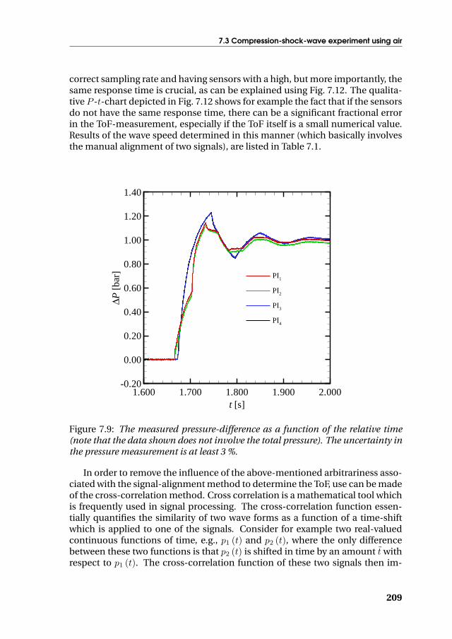
7.3 Compression-shock-wave experiment using air
correct sampling rate and having sensors with a high, but more importantly, thesame response time is crucial, as can be explained using Fig. 7.12. The qualita-tive P -t-chart depicted in Fig. 7.12 shows for example the fact that if the sensorsdo not have the same response time, there can be a significant fractional errorin the ToF-measurement, especially if the ToF itself is a small numerical value.Results of the wave speed determined in this manner (which basically involvesthe manual alignment of two signals), are listed in Table 7.1.
t [s]
ΔP[b
ar]
1.600 1.700 1.800 1.900 2.000-0.20
0.00
0.20
0.40
0.60
0.80
1.00
1.20
1.40
PI1
PI2
PI3
PI4
Figure 7.9: The measured pressure-difference as a function of the relative time(note that the data shown does not involve the total pressure). The uncertainty inthe pressure measurement is at least 3 %.
In order to remove the influence of the above-mentioned arbitrariness asso-ciated with the signal-alignment method to determine the ToF, use can be madeof the cross-correlation method. Cross correlation is a mathematical tool whichis frequently used in signal processing. The cross-correlation function essen-tially quantifies the similarity of two wave forms as a function of a time-shiftwhich is applied to one of the signals. Consider for example two real-valuedcontinuous functions of time, e.g., p1 (t) and p2 (t), where the only differencebetween these two functions is that p2 (t) is shifted in time by an amount t withrespect to p1 (t). The cross-correlation function of these two signals then im-
209

Chapter 7. Commissioning of the FAST
Table 7.1: The time-of-flight (ToF) determined in three different ways, the dis-tance between the dynamic pressure instruments (∆) and the wave speed (b)for a CSW-test performed in the FAST with air. Pressure instrument 1 is locatedthe nearest to the nozzle throat whereas pressure instrument 4 is located thefurthest. Note that average wave speeds are employed because the frontrunnerwave accelerates.
Tag PI1 PI2 PI3 PI4
From signal alignment: PI1 – 0.470 6.58 7.03ToF [ms] PI2 0.470 – 6.11 6.56uncertainty = 5.65 µs PI3 6.58 6.11 – 0.450
From cross-correlation: PI1 – 0.484 6.59 7.04ToF [ms] PI2 0.484 – 6.11 6.56
PI3 6.59 6.11 – 0.448
From squared-difference PI1 – 0.492 6.58 7.04method: PI2 0.492 – 6.11 6.56ToF [ms] PI3 6.58 6.11 – 0.452
∆ [cm] PI1 – 30.0 450 480PI2 30.0 – 420 450PI3 450 420 – 30.0
From signal alignment: PI1 – 638 684 683〈b〉 [m/s] PI2 638 – 687 686
PI3 684 687 – 667
From cross-correlation: PI1 – 620 683 682〈b〉 [m/s] PI2 620 – 687 686
PI3 683 687 – 670
From squared-difference PI1 – 610 684 682method : PI2 610 – 687 686〈b〉 [m/s] PI3 684 687 – 664
210

7.3 Compression-shock-wave experiment using air
ToF12 = 0.470 ms
ToF14 = 7.03 ms
ToF34 = 0.450 ms
ToF23 = 6.11 ms
Reflected wave
t [s]
ΔP[b
ar]
1.665 1.670 1.675 1.680-0.05
0.00
0.05
0.10
0.15
0.20
Figure 7.10: Zoomed: The measured pressure-difference as a function of the rela-tive time. Also included are values of the time-of-flight (ToF) between the variousdynamic-pressure instruments. The charge-tube pressure is equal to 0.020 bar±5.8 % (probably an even higher uncertainty), the atmospheric pressure is equalto 1.0 bar±5.8 % and the temperature of the experiment is 27± 0.40 oC. The datasampling rate is 250 kHz and the sensor bandwidth is 150 kHz. The line-legendis indicated in Fig. 7.9.
plies shifting p2 (t) with respect to p1 (t) by a predetermined value and calcu-lating the integral of the product of the two signals. By continuing the shift, ifthe two functions match, the integral of the product exhibits a maximum; themaximum occurs at a time-shift of t. In the case of discrete signals however, asare the dynamic pressure data recorded by instruments PI1 and PI2, i.e., P1,i andP2,i, the cross correlation r between these sets is defined as
r(tj)
=
∑i
(P1,i − 〈P1〉)×(P2,i−tj − 〈P2〉
)N
, (7.1)
211

Chapter 7. Commissioning of the FAST
x
t
Atmospheric pressure
Pressure in charge tube
CSW CS
RF (unsteady)
S 1 34
2
Diaphragm
t
P
Arbitrary shift by ΔP (for visualization purpose only)
PI2
PI1
ToF
Figure 7.11: Sketch of the x-t-diagram for the compression shock experiment withair. Also shown are expected recordings from the dynamic pressure instrumentsPI1 and PI2. Note that the air, once the diaphragm ruptures, flushes into the pipe,where it reaches sonic conditions, S, at a location slightly to the right of the inlet.From the sonic point onward, the flow expands further by means of unsteadyrarefaction waves. Ahead of these rarefaction waves is the CS and the CSW.
where the 〈 〉-symbol indicates the mean value of the corresponding series and
N =√∑
i
(P1,i − 〈P1〉)2
√∑i
(P2,i−tj − 〈P2〉
)2
. (7.2)
212

7.3 Compression-shock-wave experiment using air
Sensor 1 Sensor 2
Choice A Choice B
Choice A Choice B
Choice AChoice B
-3.3 % -3.1 %
-0.5 % +2.6 %
Figure 7.12: Qualitative chart illustrating the influence of the sensor responsetime-constant and the influence of the data sampling rate. The black lines rep-resent the ideal signal, whereas the green lines represent the sampled signals. Ifthe signal-alignment method is used, then, depending on choice A or B, the un-certainty in the ToF-measurement is indicated.
The value of tj for which r(tj)
is maximal, indicates maximal correlation be-tween the two signals P1 and P2, therefore, the thus obtained value of tj cor-responds to the ToF between, in this case, P1,i and P2,i. For discrete data theprocedure to determine the cross correlation r
(tj)
requires the identification ofa time window because only data in this window are used to maximize r. How-ever, cross correlation yields a series which has twice the length of the originalseries. Therefore, it must be decided what to do with data to the left and right ofthe window. Here, as is the common approach, data points outside the selectedwindow are set to zero. Results of ToF-data determined using signal cross corre-lation are also listed in Table 7.1. An uncertainty is not assigned to the ToF-valuedetermined using the cross-correlation method, because here specifically, thetime window also influences the uncertainty because of the fact that the signalsdepicted in Fig. 7.10 do not exhibit stable pre- and post shock pressures butrather the post-shock pressure increases with time. Moreover, the post-shockpressure-increase of PI1 has a different slope than that of PI2. Consequently,the cross-correlation functions which should be a triangle that exhibits a max-
213

Chapter 7. Commissioning of the FAST
imum at the ToF, has a distorted triangular shape, making an estimate of theToF-uncertainty in this case difficult.
Alternatively, a technique which is similar to least-square fitting can be used.The procedure is analogous to the cross-correlation method with the only dif-ference that the objective function, namely
F =∫T
(f (t)− g
(t− t
))2dt, (7.3)
is minimized. The interval T represents an appropriately selected time windowwhich encloses the shock wave. Since discrete signals are involved, the tj forwhich the series,
F(tj)
=M∑k=1
(f (tk)− g
(tk − tj
))2, (7.4)
albeit in its normalized form, displays a minimum, corresponds to the ToF. Us-ing this procedure, ToF’s for all the pressure signals displayed in Fig. 7.10 arecomputed and are indicated in Table 7.1.
So in summary,Treservoir 26.3 ± 0.400 oCTcharge−tube 27.0 ± 0.400 oCPreservoir 1.0 ± 0.058 barPcharge−tube 0.020 ± 0.0012–0.020 barc 349 ± ∼5 m/sToF1,2 0.470 ± 5.65 µsToF1,4 7.03 ± 5.65 µs〈b〉1,2 638 ± ∼8 m/s〈b〉1,4 683 ± ∼0.5 m/sMa1,2 1.828 ± 0.035 (1.9 %) –Ma1,4 1.957 ± 0.028 (1.4 %) –
Finally, it is to be noted that the average wave speed determined using instru-ments PI1 and PI2 between the three methods do not agree well, if the uncer-tainty of 8 m/s is considered for 〈b〉1,2 determined using the alignment method.This can also be stated for 〈b〉1,4 considering the uncertainty of 0.5 m/s. How-ever, a 1 m/s difference is acceptable.
214

7.3 Compression-shock-wave experiment using air
tj [ms]
F[x
107ba
r2 ]
R[x
102ba
r2 ]
6.70 6.80 6.90 7.00 7.10 7.20 7.30 7.40-0.5
0.0
0.5
1.0
1.5
-2.0
0.0
2.0
4.0
6.0
Figure 7.13: Results of the squared-difference method F (indicated by squares)and the cross-correlation technique R = r × N (indicated by circles) applied toPI1 and PI4. The minimum, respectively maximum, is located at tj = 7.04 mswhich corresponds to the ToF.
215

Chapter 7. Commissioning of the FAST
VAPOR GENERATOR + HEATING ELEMENT
REFERENCE TUBE
PNEUMATIC VALVE
CHARGE TUBE + HEATING ELEMENT
CONDENSER DRAIN (INCLINED PIPE)
SLIDING SUPPORT
Figure 7.14: Picture of the tank in which the test fluid is charged and vaporized.Behind it, the horizontally positioned RT can be seen. Also notice the sliding sup-ports of the charge tube and the vapor generator.
216

7.3C
om
pre
ssion-sho
ck-wa
veexp
erim
entusing
air
LOW-PRESSURE RESERVOIR + HEATING ELEMENTS
CHARGE-TUBE SEGMENTS + HEATING ELEMENTS
DAQ&C CABINET CONDENSER (UNDERNEATH RESERVOIR)
Figure 7.15: The Flexible Asymmetric Shock Tube (FAST), as built. Main assemblies are labeled. Ryan is not shown.
217
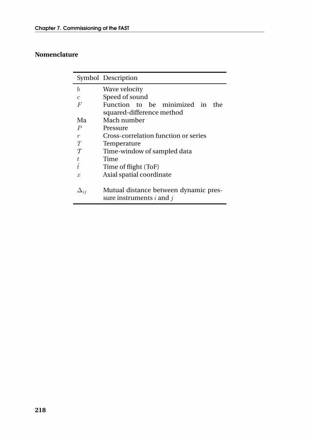
Chapter 7. Commissioning of the FAST
Nomenclature
Symbol Description
b Wave velocityc Speed of soundF Function to be minimized in the
squared-difference methodMa Mach numberP Pressurer Cross-correlation function or seriesT TemperatureT Time-window of sampled datat Timet Time of flight (ToF)x Axial spatial coordinate
∆ij Mutual distance between dynamic pres-sure instruments i and j
218

“There is no doubt in my mind when history was written, the finalpage will say: Victory was achieved by the United States of Americafor the good of the world.”
President George W. Bush, Camp Arifjan, Kuwait, January 12, 2008
8Conclusions and recommendations
for future research
8.1 Conclusions
The study documented herein has shown that it is both theoretically and tech-nically possible to create an unsteady nonclassical expansion shock wave in apolyatomic substance classifying as a Bethe-Zel’dovich-Thompson (BZT) fluid.This has resulted in the design and building of the Flexible Asymmetric ShockTube (FAST) – a unique facility for high-temperature gas-dynamic experimentsin organic fluids – equipped with a novel fast-opening valve. To this purpose,it was first of all necessary to identify potential BZT candidate fluids featur-ing several thermophysical and technological characteristics which make themsuitable for an experiment aiming at the demonstration of nonclassical gas-dynamic phenomena. This requires sophisticated thermodynamic modeling ofthe fluid, taking into account other aspects, like fluid flammability and toxicity,costs and thermochemical stability of the substance. Based on a previous studydocumented by Colonna and Silva [37], the use of model equations of state(EoS’s) showed that selected fluids within the dimethylsiloxanes family exhibitan embedded region of negative nonlinearity. However, as indicated in Ref. [37],the predictions of Γ were significantly affected by the large uncertainty in theideal-gas isobaric heat capacity correlation, viz. 25 %. Therefore, as reported inthis thesis, firstly, acoustic resonance frequency measurements were conductedyielding accurate speed-of-sound data. Using these measurements and results
219

Chapter 8. Conclusions and recommendations for future research
obtained from ab initio calculations, accurate ideal-gas isobaric heat capacitieswere predicted which have an estimated uncertainty of no more than 5–6 %.With these data and thermal and caloric property data documented elsewhere,modern EoS’s formulated in terms of the Helmholtz free energy have been de-veloped. Using these new multiparameter EoS’s, but also model EoS’s, e.g., thePeng-Robinson, Stryjek-Vera modified cubic EoS, it has been found that MD3Mand linear dimetylsiloxanes of greater molecular complexity and D6 and cyclicdimetylsiloxanes of greater molecular complexity qualify as BZT fluids, even ifthe uncertainty in the heat capacity correlation is taken into consideration (seeRef. [30]).
The fundamental derivative of gas dynamics Γ, i.e., the thermodynamic prop-erty that governs the qualitative and quantitative behavior of compressible flows,cannot be obtained easily by direct measurements in the dense-gas region whichis of interest, since Γ is a higher-order derivative of primary thermodynamicproperties. Consequently, Γ must be determined from thermodynamic models(also refer to the discussion in Chap. 4). Previous studies however, have shown ahigh degree of uncertainty in computations of Γ, if relatively simple thermody-namic models are employed. It was therefore necessary to assess if Γ could in-deed be calculated with the accuracy which is required for the design of a facilityto demonstrate BZT effects, such as the FAST. This required a study whereby thereference equations of state (EoS’s) developed for molecularly complex fluidswere used as a benchmark. The performance of simple EoS’s, like cubic EoS’swhich currently have to be employed out of necessity due to the unavailabilityof experimental thermal and caloric property data for the thermodynamic mod-eling of potential BZT candidates, was then assessed against the reference EoS’s.Additionally, this study allowed for estimating an uncertainty with which sim-ple EoS’s can predict Γ. The main findings of this study documented in Chap. 4were that:
1. If highly accurate thermodynamic models are employed, Γ can be calcu-lated with a degree of uncertainty that is suitable for dense-gas applica-tions.
2. For fluids made of complex molecules, it is possible to achieve a compara-tively higher level of accuracy in the estimation of Γ with respect to molec-ularly simpler fluids, if experimental data are available. If a sufficient num-ber of accurate experimental data are available, technical multiparameterEoS can be developed and result in an appreciable improvement with re-spect to the uncertainty of the estimation of Γ.
In addition, using scaled fundamental equations it is found that the region ofnegative nonlinearity is located partly in the critical region and is therefore un-der the influence of critical phenomena (critical anomalies). Application of thescaled fundamental equation of methane, water and carbon dioxide has yieldedthat in the single-phase critical region of these pure fluids, Γ diverges weakly to
220

8.1 Conclusions
+∞, which confirms Emanuel’s result documented in Ref. [61]. However, us-ing thermodynamic relations developed for the two-phase region of a singlecomponent fluid, use of the scaled fundamental equation of methane displays aweak divergence of Γ to−∞, which to the knowledge of the author is new result.Since the physical behavior of pure fluids near the vapor-liquid critical point isuniversal, it is believed that all fluids display a Γ < 0-region in the two-phasenear-critical region. Therefore, in principle expansion shock waves, includingexpansion-condensation shock waves are possible if thermodynamic equilib-rium between two homogeneously dispersed phases is assumed.
An investigation on possible options to demonstrate phenomena which en-sue from negative values of Γ, namely BZT effects, has been conducted and hasyielded various theoretically feasible options. Based on a comparative analy-sis whereby arguments for and against each experimental option/strategy havebeen assessed (the assessment was based on aspects like, accuracy require-ments, repeatability and reproducibility of the experiments, availability of thefacility, costs, etc.), a setup has been chosen, designed and built that aims at theproduction of an unsteady rarefaction shock wave with maximal supersonic-to-sonic speed change. The experimental facility, namely the previously men-tioned Flexible Asymmetric Shock Tube, incorporates both the operational as-pects of a simple shock tube and a Ludwieg tube.
The facility as built has been tested; during the commissioning phase vari-ous tests have been done to ensure the structural integrity of the facility and tocheck whether all specifications are met. To this purpose, a temperature con-trol test has been performed aimed at firstly, the determination of optimal PID-control parameters and secondly, if using these parameters, tight temperaturecontrol of the shock tube and the balance of plant can be achieved. The secondset of tests that was done was related to the measurement of the time-of-flightof a created unsteady classical compression shock wave in air. Both these setsof tests were successful, since it was possible to regulate the temperature of thecharge tube to within 0.01 oC and the wave Mach number, which in turn de-pends also on the time-of-flight, could be computed with an uncertainty of lessthan 2 %. It is expected that in the case of rarefaction-shock-wave experimentsin siloxanes, the Mach number can be computed with a lower uncertainty, be-cause, due to the lower wave speeds, the relative uncertainty in the time-of-flight measurement is less than that in air for the given instrumentation andfacility.
There are however some open questions which can only be answered oncethe experiment is conducted in the FAST. For example, the flow Reynolds num-ber past the generated wave train, which develops as the fast-opening valve isopened, may cause the rarefaction wave never to coalesce into a shock wave.This conclusion can only be drawn after many repeated runs of experiments.Furthermore, many polyatomic gases exhibit a single vibrational relaxation pro-cess. If this is also assumed for BZT fluids, then relaxation was found to occurcompletely inside the shock wave and not downstream of it. However, vibra-
221

Chapter 8. Conclusions and recommendations for future research
tional relaxation can also be nonlinear and currently, nothing is known aboutvibrational relaxation in dimethylsiloxanes classifying as BZT fluids, like D6,therefore relaxation can potentially complicate the flow field.
8.2 Recommendations
Soon,1 experiments aimed at generating nonclassical unsteady rarefaction shockwaves will be performed using the FAST. This will require a trial and error proce-dure because, due to the presence of a transitional or turbulent boundary layerquite close to the wave and due to the uncertainty of the thermodynamic EoS ofthe fluid, the opening of the nozzle’s throat (which is built into the fast-openingvalve) is to be tuned. Also the setting of the correct initial states prior to theopening of the valve, viz. the pressures and temperatures in the charge tubeand the low-pressure reservoir, is crucial. There are still some open questions,e.g., it is not known if the initially formed rarefaction wave even coalesces intoa shock wave due to the potentially strong boundary layer immediately behindthe frontrunner wave, or, if a shock wave is indeed formed, whether or not itattenuates and disperses into a sonic wave before it reaches the dynamic pres-sure instruments. Furthermore, nonlinear vibrational relaxation may pose ad-ditional complications and, in the worst case, thermochemical decompositionof the working fluid can occur. All these aspects can only be discussed in moredetail once tests are performed under the exact experimental conditions.
Aside from the envisaged rarefaction-shock-wave tests, research in the near-future should be aimed at the theoretical, numerical and experimental study of:
1. The application of BZT fluids and the exploitation of nonclassical gas dy-namic phenomena in organic Rankine cycle engines (ORCE’s)
ORCE’s are small energy conversion systems of the order of a few kilo-Watts (30 kW) to a few MegaWatts (1–3 MW), for decentralized terres-trial and space applications (see Angelino and Invernizzi [7] and refer-ences therein). The working principle of ORCE’s is the same as that of con-ventional steam Rankine power cycles, with the main difference that theworking fluid is an organic compound instead of water. Currently, non-BZT fluids such as the dimethylsiloxanes MM and MDM, are employed asworking fluids in ORCE’s and it is in principle possible to develop and de-sign power units which employ more molecularly complex substances ofthe same fluid family, e.g., D6 which classifies as a BZT fluid. Due to thehigh molecular weight of a fluid such as D6 however, the optimal poweroutput for which the ORCE can be designed, is low, e.g., of the order of 2–3kWe (with co-generation, the total power output is up to 12 kW). Never-theless, the nonclassical gas dynamic phenomena which ensue from the
1Update: 26 March 2009
222

8.2 Recommendations
fact that D6 has an embedded region of negative-Γ, can be exploited inorder to improve the cycle efficiency. The concept of exploiting BZT ef-fects in ORC-turbines is based on earlier, more fundamental, studies con-ducted by Cramer and Park [49] and Kluwick [113]. By solving the com-pressible Navier-Stokes equations coupled to a real-gas thermodynamicmodel, Cramer and Park [49] demonstrated, using a benchmark problemof the reflection of an oblique shock wave from a laminar boundary layeron a flat adiabatic plate, that, if a BZT fluid was expanded under simi-lar pressure and temperature conditions as what is encountered in ORC-turbines, boundary layer separation did not occur. The suppression ofboundary layer detachment was the result of the fact that compressionshock waves were inadmissible and, in fact, they disintegrated instead intosmooth compression fans. Additionally, it was found that the pressure-gradient is more important regarding boundary layer detachment than theoverall compressive pressure change and thus detachment of the bound-ary layer does not occur if the fan is smooth enough. If an expansion shockwave was admitted, there was no adverse pressure gradient and thereforethe boundary layer remained attached. Thus the study of Cramer andPark shows that it is possible to eliminate the loss mechanisms in ORC-turbines if the turbine inlet and outlet conditions are well-chosen. Brownand Argrow [19] extended this work further and conducted a proof-of-concept study of the exploitation of BZT effects in ORCE’s. The potentialturbine-efficiency improvement was assessed in a two-dimensional cas-cade analysis using a real cascade geometry of a symmetric impulse tur-bine and both a supersonic inlet and outlet. The outcome of Brown andArgrow’s [19] investigation was that if only the irreversible effects due tothe presence of shock waves was accounted for, the efficiency improve-ment of the ORC-turbine could be as high as 3 %, notwithstanding the factthat greater improvements are possible if also losses due to boundary layerdetachment are considered.
The limitation of these studies is that only the turbine is considered andnot the thermodynamic performance of the cycle as a whole. The compu-tations of the efficiency improvements for example should be done tak-ing the entire cycle into account and not only improving the efficiency ofone component and deteriorating the overall cycle performance. Also theoff-design behavior must be included in the assessment of the proof-of-concept especially because of the fact that ORCE’s often operate in part-load conditions. It is in part-load conditions that BZT effects may be mostsuitable.
2. Nonclassical gas dynamics in mixtures classifying as BZT fluids
In the study conducted by Colonna and Silva [37] it was demonstrated us-ing the Peng-Robinson, Stryjek-Vera modified, cubic EoS combined with
223

Chapter 8. Conclusions and recommendations for future research
the Wong-Sandler mixing rules, that mixtures of siloxanes can exhibit a re-gion of Γ < 0 in the single-phase dense-gas regime. This work should beextended to other mixtures, e.g., perfluorocarbon-siloxane mixtures. It isexpected that due to the additional degree of freedom, namely the com-position, the interval of thermodynamic states that exhibit Γ < 0-valuescan be tuned. Initially, the investigation of BZT effects in mixtures shouldbe mostly theoretical.
3. Nonclassical gas dynamics in the near-critical single- and two-phase re-gion of pure fluids
It was demonstrated in Sec. 4.5 that the fundamental derivative of gas dy-namics exhibits anomalous behavior as the vapor-liquid critical point ofa single-component fluid is approached. Since in the vapor-liquid equi-librium (VLE) region, Γ diverges to −∞, rarefaction shock waves featur-ing vapor-liquid phase transition are admissible, as can be demonstratedusing the shock admissibility conditions. That Γ is negative in the two-phase region close to the critical point may also be of use in studies re-lated to atomization (for example of fuel in internal combustion engines),and in studies on spray-drying for producing particles with supercriticalCO2. In the last-mentioned process for example, the density gradient isan important parameter which determines the particle size. Near-criticalshock waves must also be investigated from a theoretical viewpoint whereone must account for the validity of the assumptions of thermodynamicequilibrium between homogeneously dispersed phases. Once the the-oretical aspects are well-understood, experiments should be conductedto demonstrate near-critical expansion shock waves, in particular thosedisplaying condensation. These types of experiments can be conductedat relatively low temperature, like at room temperature, because unlikethe negative nonlinearity region in the single-phase dense-gas regime, thenegative value of Γ in the near-critical VLE-region is independent of themolecular complexity of the substance. These experiments can be donewith the FAST, however, the influence of gravity must be assessed.
Remark that Γ → ±∞ from a physical viewpoint, is meaningless. In fact,Γ will just becomes arbitrarily large as the critical point is approached andlevels off to a fixed, large value.
Finally, thermodynamic modeling of the working fluid is important, not onlyfor the design of an experiment and determination of the thermodynamic statesprior to a run, but also for the design and analysis of a technical application thatcan exploit BZT effects. Thermodynamic data for potential BZT fluids howeverare scarce, mostly because measurements have to be done at elevated temper-atures and a general lack of interest of knowing the thermodynamic propertiesin the dense-gas region of molecularly complex fluids, such as dimethylsilox-
224

8.2 Recommendations
anes and perfluorocarbons. Future work thus has to include the measurementof thermal and caloric property data of molecularly complex fluids in the dense-gas and critical region, in particular the siloxanes considered in this study.
Nomenclature
Symbol Description
Γ Fundamental derivative of gas dynamics
225


“There’s an old saying in Tennessee – I know it’s in Texas, probablyin Tennessee – that says, fool me once, shame on – shame on you.Fool me – you can’t get fooled again.”
President George W. Bush, Nashville, Tennessee, September 17,2002
AExperimental speed-of-sound data
for fluids D4, [(CH3)2-Si-O]4, and D5,[(CH3)2-Si-O]5
The following tables list speed-of-sound values for octamethylcyclotetrasilox-ane and decamethylcyclopentasiloxane, that were measured at NIST, Gaithers-burg, MD, during the period between 15 September 2005–15 November 2005.Relevant information can be found in Chap. 3, including the nomenclature.
Table A.1: Experimental speed-of-sound data for D4 at certain values for pres-sure and temperature. The experimental uncertainties are also listed.
T [K] P [kPa] c [m/s] 104 · σu [m/s]
450 38.90 110.351 252.046.70 109.656 89.857.41 108.801 72.262.89 108.299 17.069.33 107.727 16.4
465 31.29 113.043 638.940.99 112.320 123.049.18 111.723 69.258.99 110.976 20.2
Continued on the next page. . .
227

Chapter A. Experimental speed-of-sound data for fluids D4, [(CH3)2-Si-O]4, and D5,[(CH3)2-Si-O]5
Table A.1 – Continued
T [K] P [kPa] c [m/s] 104 · σu [m/s]
70.69 110.062 16.577.48 109.530 24.992.89 108.286 9.9
101.01 107.535 14.3111.40 106.695 5.3121.67 105.761 7.4
465 36.51 112.753 138.647.85 111.913 37.257.21 111.202 25.368.51 110.332 14.474.87 109.829 10.781.72 109.278 26.597.68 107.963 270.8
106.95 107.179 89.7116.93 106.300 335.1
465 32.63 112.986 242.546.84 111.935 53.361.46 110.824 18.873.59 109.872 15.387.87 108.720 9.0
105.11 107.277 15.0123.48 105.664 17.4
480 42.70 114.022 56.254.67 113.202 18.165.08 112.478 36.171.30 112.038 24.685.50 111.071 24.992.46 110.502 12.1
109.21 109.241 4.5118.88 108.493 3.1129.21 107.675 6.8140.39 106.769 11.2152.36 105.769 8.6165.42 104.642 6.3
495 27.45 117.135 200.836.20 116.658 71.647.54 115.985 15.6
143.41 109.744 283.3159.70 108.434 20.5160.40 108.391 105.0
Continued on the next page. . .
228

Table A.1 – Continued
T [K] P [kPa] c [m/s] 104 · σu [m/s]
174.53 107.346 44.6186.64 106.439 78.7198.61 105.492 1287.4224.52 103.408 31.8
Table A.2: Experimental speed-of-sound data for D5 at certain values for pres-sure and temperature. The experimental uncertainties are also listed.
T [K] P [kPa] c [m/s] 104 · σu [m/s]
485 82.92 97.275 62.364.42 99.132 101.449.43 100.666 75.2
485 85.12 97.170 56.774.85 98.380 97.063.60 99.197 119.955.24 100.360 44.543.63 101.141 450.635.39 101.908 238.9
500 116.60 96.555 219.5105.42 97.603 59.0
95.37 98.558 54.085.90 99.495 65.574.95 100.631 17.964.64 101.500 31.955.42 102.199 161.542.70 103.271 134.233.93 103.964 215.726.30 104.683 16.3
500 78.98 100.217 28.647.88 102.870 32.731.33 104.222 75.422.48 104.919 126.8
500 73.64 100.810 63.464.96 101.440 122.651.58 102.577 0.639.90 103.532 26.232.27 104.140 11.9
Continued on the next page. . .
229

Chapter A. Experimental speed-of-sound data for fluids D4, [(CH3)2-Si-O]4, and D5,[(CH3)2-Si-O]5
Table A.2 – Continued
T [K] P [kPa] c [m/s] 104 · σu [m/s]
22.13 104.938 0.0510 110.69 99.980 120.1
89.89 100.871 49.557.10 103.487 52.734.55 105.200 31.7
510 103.28 99.891 82.592.75 100.754 5.982.51 101.583 20.372.53 102.369 5.462.78 103.980 261.951.27 104.860 55.743.26 104.679 19.2
230

“As Luce reminded me, he said, without data, without facts, with-out information, the discussions about public education mean that aperson is just another opinion.”
President George W. Bush, Jacksonville, Florida, September 9, 2003
BRelevant expressions for computing
the fundamental derivative of gasdynamics from a canonical
Helmholtz function
For the computation of the fundamental derivative of gas dynamics and otherthermodynamic properties, first-order, second-order, and composite deriva-tives of pressure with respect to specific volume and temperature are required.Expressions for the computation of thermodynamic properties from a canon-ical Helmholtz equation of state are presented in the following (see also Span[184] and Colonna et. al. [30]). The Helmholtz function can be formulated as(refer to Chap. 4 for the nomenclature) Ψ (T, ρ) / (RT ) =
[ψ0 (τ, δ) + ψR (τ, δ)
],
where δ ≡ ρ/ρC = vC/v and τ ≡ TC/T . The ideal-gas part of the reducedHelmholtz function is
ψ0 (τ, δ) =h0
0τ
RTC− s0
0
R− 1 + ln
(τ0δ
δ0τ
)− τ
R
τ∫τ0
C0P
τ2dτ +
1R
τ∫τ0
C0P
τdτ , (B.1)
where δ0 = ρ0/ρC and τ0 = TC/T0 and represent the reduced density and theinverse of the reduced temperature, respectively at a pre-defined or prescribedreference state (T0, ρ0). The values of h0
0 and s00 (at the reference temperature T0
and specific volume v0) are chosen based on recommendations of the Interna-
231

Chapter B. Relevant expressions for computing the fundamental derivative of gas dynamicsfrom a canonical Helmholtz function
tional Union of Pure and Applied Chemistry (IUPAC) or according to conven-tions used in industry.
The pressure is determined from
Pv
RT= Z = 1 + δ
(∂ψR
∂δ
)τ
, (B.2)
and the pressure derivatives are computed from(∂P
∂v
)T
=− RT
v2
[1 + 2δ
(∂ψR
∂δ
)τ
+ δ2
(∂2ψR
∂δ2
)τ
](B.3)
(∂P
∂T
)v
=R
v
[1 + δ
(∂ψR
∂δ
)τ
− δτ(∂2ψR
∂τ∂δ
)τ,δ
](B.4)
(∂2P
∂v2
)T
=RT
v3
[2 + 6δ
(∂ψR
∂δ
)τ
+ 6δ2
(∂2ψR
∂δ2
)τ
+ δ3
(∂3ψR
∂δ3
)τ
](B.5)(
∂2P
∂T∂v
)T,v
=R
v2
[τδ
{2(∂2ψR
∂τ∂δ
)δ,τ
+ δ
(∂3ψR
∂τ∂2δ
)δ,τ
}]−
R
v2
[{1 + 2δ
(∂ψR
∂δ
)τ
+ δ2
(∂2ψR
∂δ2
)τ
}](B.6)
(∂2P
∂T 2
)v
=R
Tv
[δτ2
(∂3ψR
∂τ2∂δ
)τ,δ
]. (B.7)
The isochoric specific heat and its first-order derivative with respect to the tem-perature read
Cv =−Rτ2
[(∂2ψ0
∂τ2
)δ
+(∂2ψR
∂τ2
)δ
](B.8)
(∂Cv∂T
)v
=Rτ
T
[2τ(∂2ψ0
∂τ2
)δ
+ 2τ(∂2ψR
∂τ2
)δ
+ τ2
(∂3ψ0
∂τ3
)δ
]+
Rτ
T
[τ2
(∂3ψR
∂τ3
)δ
]. (B.9)
The fundamental derivative of gas dynamics can then be computed from
Γ =v3
2c2
{(∂2P
∂v2
)T
− 3T
Cv
(∂P
∂T
)v
(∂2P
∂v∂T
)+[T
Cv
(∂P
∂T
)v
]2
× (B.10)
[3(∂2P
∂T 2
)v
+1T
(∂P
∂T
)v
(1− T
Cv
(∂Cv∂T
)v
)]}.
232

“I can only speak to myself.”
President George W. Bush,Washington, D.C., April 28, 2005
CEquations valid in the critical region –
The revised and extended linearmodel
According to theory, the thermodynamic behavior of fluids near the critical pointcan be described using a scaled fundamental equation with universal critical ex-ponents (refer to Table C.1) and system-dependent constants [180]. The scaledfundamental equation adopted herein uses the functional form proposed byBalfour et al. [10] (refer to Chap. 4 for the nomenclature). The functional formis expressed in terms of the intensive (field) variables pressure P , temperatureT and chemical potential µ and reads:
P = 1 +3∑i=1
Pi
(∆T)i
+ ∆µ(
1 + P11∆T)
+ ∆P , (C.1)
with
∆T = T + 1 (C.2)
and
∆µ = µ− µC −4∑i=1
µi
(∆T)i, (C.3)
233

Chapter C. Equations valid in the critical region – The revised and extended linear model
Table C.1: Values of universal constants in the revised and extended linearmodel (see also Ref [125]).
β = 0.325 δ = 4.82b2 = 1.3757 ∆1 = 0.50p00 = 0.586535 p20 = −1.026243p40 = 0.612903 p01 = 0.10325p21 = 0.16032 p41 = −0.16986s00 = 1.109430 s20 = −1.981395s01 = 0.24692 s21 = −0.84341
whereby
T ≡ −TC
T, µ ≡ µ
T
ρCTC
PC, P ≡ P
T
TC
PC. (C.4)
In Eqns. (C.1)-(C.4), Pi and P11 are the pressure background constants and theseare specific to a fluid, µi are referred to as the thermal background constantsand are also substance specific, ρ denotes the density, and subscript “C” repre-sents the critical-point value of a property. The critical-point singularities areaccounted for by the ∆P -term in Eq. (C.1). This singular part of the scaled fun-damental equation is expressed as a function of so-called parametric variablesr and θ; the variable denoted by r gives the distance of a thermodynamic statewith respect to the critical point and the variable denoted by θ gives the loca-tion of the thermodynamic state on a line of constant-r, such that θ = −1 is thedew-line and θ = +1 is the bubble-line (−1 ≤ θ ≤ +1). From the fundamentalequation, i.e., Eq. (C.1), all other thermodynamic properties can be determinedusing the relationships (C.5)–(C.12).
234

ρ
ρC=[1 + P11∆T + ∆P∆µ
](C.5)
ρC
PC
(∂P
∂ρ
)T
=−
[ρ
T∆P∆µ,∆µ
](C.6)
TC
PC
(∂P
∂T
)ρ
=− T
3∑i=1
iPi
(∆T)i−1
+ P11∆µ+ ∆P∆T − ρ
(P11 + ∆P∆µ,∆T
)∆P∆µ,∆µ
− P
T
(C.7)
ρ2C
PC
(∂2P
∂ρ2
)T
=−
[∆P 2
∆µ,∆µ − ρ∆P∆µ,∆µ,∆µ
T∆P 3∆µ,∆µ
](C.8)
T 2C
PC
(∂2P
∂T 2
)ρ
=− T 3
3∑i=2
i (i− 1) Pi(
∆T)i−2
−
(P11 + ∆P∆µ,∆T
)2
∆P∆µ,∆µ
−ρ∆P∆µ,∆T ,∆T
∆P∆µ,∆µ
− T 3∆P∆T ,∆T −
T 3ρ(P11 + ∆P∆µ,∆T
)∆P 2
∆µ,∆µ
×∆P∆µ,∆µ,∆T + ∆P∆µ,∆T ,∆µ −∆P∆µ,∆µ,∆µ
(P11 + ∆P∆µ,∆T
)∆P∆µ,∆µ
(C.9)
235

Cha
pte
rC.Eq
uatio
nsva
lidin
thec
ritica
lreg
ion
–The
revised
and
extend
ed
linea
rmo
de
l
ρCTC
PC
(∂2P
∂ρ∂T
)ρ,T
=ρ
∆P∆µ,∆µ
1 +T
∆P∆µ,∆µ
∆P∆µ,∆T ,∆µ −∆P∆µ,∆µ,∆µ
(P11 + ∆P∆µ,∆T
)∆P∆µ,∆µ
(C.10)
ρCTC
PCCv =
T 2
ρ
3∑i=2
i (i− 1) Pi(
∆T)i−2
+ ∆P∆T∆T −
(P11 + ∆P∆µ,∆T
)2
∆P∆µ,∆µ
− T 2
4∑i=2
i (i− 1) µi(
∆T)i−2
(C.11)
ρCT2C
PC
(∂Cv∂T
)ρ
=T 4
ρ
3∑i=3
i (i− 1) (i− 2) Pi(
∆T)i−3
+ ∆P∆T ,∆T ,∆T −
(P11 + ∆P∆µ,∆T
)∆P∆µ,∆µ
×
2∆P∆µ,∆T ,∆T −∆P∆µ,∆µ,∆T
(P11 + ∆P∆µ,∆T
)∆P∆µ,∆µ
+
(P11 + ∆P∆µ,∆T
)2
∆P 2∆µ,∆µ
×
2∆P∆µ,∆T ,∆µ −∆P∆µ,∆µ,∆µ
(P11 + ∆P∆µ,∆T
)∆P∆µ,∆µ
− ρ
4∑i=3
i (i− 1) (i− 2) µi(
∆T)i−3
−∆P∆T∆T ,∆µ
(P11 + ∆P∆µ,∆T
)∆P∆µ,∆µ
+2CvTρ
. (C.12)
236
In Eq. (C.5), ρ ≡ ρ/ρC, and in Eq. (C.12), Cv/ρ = Cv (ρCTC) /PC.The parametric equations for the singular terms (these are ∆P , ∆T , ∆µ, and
the derivatives of ∆P with respect to ∆T and ∆µ) are presented in Table C.2 andthe auxiliary functions for the parametric equations are given in Table C.3.
The equations listed in Tables C.1–C.3 together with Eqns. (C.1)–(C.12) canbe used to determine the fundamental derivative of gas dynamics, appropri-ately transformed as:
Γ = 1 +ρ
c
(∂c
∂ρ
)s
⇔ Γ =1
2c2ρ3
(Γ1 + Γ2 + Γ3
), (C.13)
where
Γ1 = ρ4
(∂2P
∂ρ2
)T
+ 2ρ3
(∂P
∂ρ
)T
, (C.14a)
Γ2 = 3Tρ2
Cv
(∂P
∂T
)ρ
(∂2P
∂ρ∂T
)T,ρ
, (C.14b)
Γ3 =
[T
Cv
(∂P
∂T
)ρ
]2
×
[3(∂2P
∂T 2
)ρ
+1T
(∂P
∂T
)ρ
(1− T
Cv
(∂Cv∂T
)ρ
)], (C.14c)
and the thermodynamic speed of sound, c, is computed from
c2 =(∂P
∂ρ
)T
+T
ρ2Cv
(∂P
∂T
)2
ρ
. (C.14d)
Other relevant caloric properties are the specific internal energy (e), the specificenthalpy (h) and the specific entropy (s):
ρC
PCe =
e
ρ=
1ρ
[3∑i=1
iPi∆T i−1 − ρ4∑i=1
iµi∆T i−1 + P11∆µ+ ∆P∆T
], (C.15)
ρC
PCh =
[e
ρ− P
T ρ
], (C.16)
ρCTC
PCs =
[P
ρ− µ− T e
ρ
]. (C.17)
237

Cha
pte
rC.Eq
uatio
nsva
lidin
thec
ritica
lreg
ion
–The
revised
and
extend
ed
linea
rmo
de
l
Table C.2: Parametric equations for the singular terms. The scaling-field param-eters a, k0, k1, and c are specific to a substance.
∆µ = arβδθ(1− θ2
)∆T = r
(1− b2θ2
)− c∆µ
∆P = arβ(δ+1)[k0p0 (θ) + r∆1k1p1 (θ)
]∆P∆T =
(∂∆P∂∆T
)∆µ
= arβ(δ+1)−1[k0s0 (θ) + r∆1k1s1 (θ)
]∆P∆µ =
(∂∆P∂∆µ
)∆T
= rβ[k0 + r∆1k1
]θ + c
(∂∆P∂∆T
)∆µ
∆P∆T ,∆T =
(∂2∆P∂∆T 2
)∆µ
= arβ(δ+1)−2[k0w0 (θ) + r∆1k1w1 (θ)
]∆P∆µ,∆µ =
(∂2∆P∂∆µ2
)∆T
= a−1rβ(1−δ)[k0u0 (θ) + r∆1k1u1 (θ)
]+
2crβ−1[k0v0 (θ) + r∆1k1v1 (θ)
]+ c2
(∂2∆P∂∆T 2
)∆µ
∆P∆µ,∆T † =
(∂2∆P
∂∆T ∂∆µ
)∆T ,∆µ
= rβ−1[k0v0 (θ) + r∆1k1v1 (θ)
]+ c
(∂2∆P∂∆T 2
)∆µ
Continued on the next page. . .
238

Table C.2 – Continued
∆P∆T ,∆T ,∆T =
(∂3∆P∂∆T 3
)∆µ
= arβ(δ+1)−3[k0x0 (θ) + r∆1k1x1 (θ)
]∆P∆µ,∆T ,∆T ? =
(∂3∆P
∂∆T 2∂∆µ
)∆T ,∆µ,∆µ
= rβ−2[k0y0 (θ) + r∆1k1y1 (θ)
]+ c
(∂3∆P∂∆T 3
)∆µ
∆P∆µ,∆T ,∆µ‡ =
(∂3∆P
∂∆µ∂∆T ∂∆µ
)∆T ,∆µ,∆T
= a−1rβ(1−δ)−1[k0z0 (θ) + r∆1k1z1 (θ)
]+
2c
(∂3∆P
∂∆T 2∂∆µ
)∆T ,∆µ,∆µ
− c2
(∂3∆P∂∆T 3
)∆µ
∆P∆µ,∆µ,∆µ =
(∂3∆P∂∆µ3
)∆T
= a−2rβ(1−2δ)[k0m0 (θ) + r∆1k1m1 (θ)
]+ c3
(∂3∆P∂∆T 3
)∆µ
−
3c2
(∂3∆P
∂∆T 2∂∆µ
)∆T ,∆µ,∆µ
+ 3c
(∂3∆P
∂∆µ∂∆T ∂∆µ
)∆T ,∆µ,∆T
† ∆P∆µ,∆T = ∆P∆T ,∆µ
? ∆P∆T ,∆µ,∆T = ∆P∆µ,∆T ,∆T = ∆P∆T ,∆T ,∆µ
‡ ∆P∆T ,∆µ,∆µ = ∆P∆µ,∆T ,∆µ = ∆P∆µ,∆µ,∆T
239

Cha
pte
rC.Eq
uatio
nsva
lidin
thec
ritica
lreg
ion
–The
revised
and
extend
ed
linea
rmo
de
l
Table C.3: Auxiliary functions used in the parametric equations listed in Ta-ble C.2. Also refer to Table C.1 listing the required universal constants.
pi (θ) = p0i + p2iθ2 + p4iθ
4 (i = 0, 1)
si (θ) = s0i + s2iθ2 (i = 0, 1)
s′i (θ) = 2s2iθ (i = 0, 1)
s′′i (θ) = 2s2i (i = 0, 1)
q (θ) = 1 +[b2(2βδ − 1
)− 3]θ2 − b2
(2βδ − 3
)θ4
q′ (θ) = 2[b2(2βδ − 1
)− 3]θ − 4b2
(2βδ − 3
)θ3
u0 (θ) =[1− b2
(1− 2β
)θ2]/q (θ)
u′0 (θ) =[−2b2
(1− 2β
)θ − u0 (θ) q′ (θ)
]/q (θ)
u1 (θ) =[1− b2
(1− 2β − 2∆1
)θ2]/q (θ)
u′1 (θ) =[−2b2
(1− 2β − 2∆1
)θ − u1 (θ) q′ (θ)
]/q (θ)
v0 (θ) =[β(1− 3θ2
)θ − βδ
(1− θ2
)θ]/q (θ)
Continued on the next page. . .
240

Table C.3 – Continued
v′0 (θ) =[β(1− 9θ2
)− βδ
(1− 3θ2
)− v0 (θ) q′ (θ)
]/q (θ)
v1 (θ) =[(β + ∆1
) (1− 3θ2
)θ − βδ
(1− θ2
)θ]/q (θ)
v′1 (θ) =[(β + ∆1
) (1− 9θ2
)− βδ
(1− 3θ2
)− v1 (θ) q′ (θ)
]/q (θ)
w0 (θ) =[(βδ + β − 1
) (1− 3θ2
)s0 (θ)− βδ
(1− θ2
)θs′0 (θ)
]/q (θ)
w′0 (θ) =[−6(βδ + β − 1
)θs0 (θ) +
(β − 1
) (1− 3θ2
)s′0 (θ)− βδ
(1− θ2
)θs′′0 (θ)
−w0 (θ) q′ (θ)] /q (θ)
w1 (θ) =[(βδ + β − 1 + ∆1
) (1− 3θ2
)s1 (θ)− βδ
(1− θ2
)θs′1 (θ)
]/q (θ)
w′1 (θ) =[−6(βδ + β − 1 + ∆1
)θs1 (θ) +
(β − 1 + ∆1
) (1− 3θ2
)s′1 (θ)
−βδ(1− θ2
)θs′′1 (θ)− w1 (θ) q′ (θ)
]/q (θ)
x0 (θ) =[(βδ + β − 2
) (1− 3θ2
)w0 (θ)− βδ
(1− θ2
)θw′0 (θ)
]/q (θ)
x1 (θ) =[(βδ + β − 2 + ∆1
) (1− 3θ2
)w1 (θ)− βδ
(1− θ2
)θw′1 (θ)
]/q (θ)
y0 (θ) =[(β − 1
) (1− 3θ2
)v0 (θ)− βδ
(1− θ2
)θv′0 (θ)
]/q (θ)
Continued on the next page. . .
241

Cha
pte
rC.Eq
uatio
nsva
lidin
thec
ritica
lreg
ion
–The
revised
and
extend
ed
linea
rmo
de
l
Table C.3 – Continued
y1 (θ) =[(β − 1 + ∆1
) (1− 3θ2
)v1 (θ)− βδ
(1− θ2
)θv′1 (θ)
]/q (θ)
z0 (θ) =[(β − 1
)2b2θv0 (θ) +
(1− b2θ2
)v′0 (θ)
]/q (θ)
z1 (θ) =[(β − 1 + ∆1
)2b2θv1 (θ) +
(1− b2θ2
)v′1 (θ)
]/q (θ)
m0 (θ) =[(β − βδ
)2b2θu0 (θ) +
(1− b2θ2
)u′0 (θ)
]/q (θ)
m1 (θ) =[(β − βδ + ∆1
)2b2θu1 (θ) +
(1− b2θ2
)u′1 (θ)
]/q (θ)
242

“I’m the decider, and I decide what is best. And what’s best is forDon Rumsfeld to remain as the Secretary of Defense”
President George W. Bush,Washington, D.C., April 18, 2006
DThermodynamic properties in theVLE-region of a single-component
fluid
The following equations are derived under the assumption that the vapor- andthe liquid phase of the single-component fluid form a homogeneous mixtureand that the two phases are always in thermodynamic equilibrium. This impliesthat there is mass and heat transfer between the phases and that the timescaleof an arbitrary process is slower than that of evaporation or condensation. Con-versely, if the timescale of an arbitrary process is faster than that of evaporationor condensation, then there is insufficient time for thermodynamic equilibriumto establish and as a result, the vapor quality cannot change (fast enough). Thespeed of sound in the vapor-liquid equilibrium (VLE) region of a single compo-nent fluid can be calculated from (refer to Chap. 4 for the nomenclature)
c$,Tsat
=
√√√√√√√−(v$,T
sat)2
$
[(dvV
dP
)−(dvL
dP
)]+ (vV − vL)
(∂$
∂P
)$,T sat
s
+(dvL
dP
) , (D.1)
where $ is the vapor quality defined as the ratio of the vapor mass with respectto the total mass of vapor and liquid (here and for all the following equationswhich contain the variable $, 0 < $ < 1; the saturated state, i.e., where $ is ei-ther 0 or 1, is the limiting situation of a thermodynamic state in the single-phase
243

Chapter D. Thermodynamic properties in the VLE-region of a single-component fluid
region1), T sat denotes the saturation temperature, P represents the pressure, vis the specific volume in the VLE-region (it is thus a function of both$ and T sat),and (
∂$
∂P
)$,T sat
s
=($ − 1sV − sL
)(dsL
dP
)−(
$
sV − sL
)(dsV
dP
), (D.2)
(dvV,L
dP
)= −
(∂P
∂T
)v=vV,L,T sat
v(∂P
∂v
)v=vV,L,T sat
T
(dP
dT
)sat+
1(∂P
∂v
)v=vV,L,T sat
T
, (D.3)
and
(dsV,L
dP
)=
Cv=vV,L
P
T sat
(dP
dT
)sat +
(∂P
∂T
)v=vV,L,T sat
v(∂P
∂v
)v=vV,L,T sat
T
. (D.4)
In Eqns. (D.2)–(D.4), s represents the entropy. Furthermore, superscipts “V” and“L” denote the vapor and liquid phase, respectively. Note that thermodynamic
functions with a ∂-symbol, like (∂P/∂T )v=vV,L,T sat
v , represent functions that de-pend on two independent variables, e.g., either
(v = vV, T sat
)or(v = vL, T sat
),
in the limit that the saturated state is approached from the single-phase region.Similarly, Cv=vV,L
P is the isobaric heat capacity of either the vapor or the liq-uid phase in the limit that the saturated state is approached from the single-phase region and consequently Cv=vV,L
P is a function of two independent ther-modynamic properties.2 However, thermodynamic functions with a d-symbol,e.g.,
(dvV,LdP
), represent functions that are dependent on only one thermody-
namic property, i.e., either the saturated pressure or temperature, and they areevaluated along a line representing saturation, for example
(dvV/dP
)is com-
puted along the dew-line in aP -v-diagram and(dsL/dP
)is calculated along the
bubble-line in a P -s-diagram. The function (dP/dT )sat is the slope of the sat-uration line in the P -T -plane and it is calculated with the Clapeyron equation
(dP
dT
)sat
=sV − sL
vV − vL. (D.5)
In the VLE-region the fundamental derivative of gas dynamics is computed from(see next page)
1Remark that certain thermodynamic properties like the speed of sound and the isochoric heatcapacity display discontinuities at phase boundaries, see for example Refs. [110, 163].
2The isobaric heat capacity in the VLE-region is meaningless.
244

Γ$,Tsat
=
(c$,T
sat)4
(v$,T sat)3
[(dvV
dP
)−(dvL
dP
)](∂$
∂P
)$,T sat
s
+
(c$,T
sat)4
2 (v$,T sat)3 ×{$
[(d2vV
dP 2
)−(d2vL
dP 2
)]+(vV − vL
)(∂2$
∂P 2
)$,T sat
s
+(d2vL
dP 2
)}, (D.6)
with
(∂2$
∂P 2
)$,T sat
s
=2(∂$
∂P
)$,T sat
s
[(dsL
dP
)−(dsV
dP
)]+ ($ − 1)
(d2sL
dP 2
)−$
(d2sV
dP 2
)sV − sL
, (D.7)
(d2vV,L
dP 2
)=
∂(dvV,L
dP
)∂v
v=vV,L,T sat
T
(dvV,L
dP
)+
∂(dvV,L
dP
)∂T
v=vV,L,T sat
v
1(dP
dT
)sat , (D.8)
(d2sV,L
dP 2
)=
∂(dsV,L
dP
)∂v
v=vV,L,T sat
T
(dvV,L
dP
)+
∂(dsV,L
dP
)∂T
v=vV,L,T sat
v
1(dP
dT
)sat , (D.9)
245

Cha
pte
rD.The
rmo
dyna
mic
pro
pe
rties
inthe
VLE-re
gio
no
fasing
le-c
om
po
nentfluid
∂(dvV,L
dP
)∂v
v=vV,L,T sat
T
= −
(∂2P
∂v∂T
)v=vV,L,T sat
v,T(∂P
∂v
)v=vV,L,T sat
T
(dP
dT
)sat
−
[(dP
dT
)sat
−(∂P
∂T
)v=vV,L,T sat
v
](dP
dT
)sat(∂2P
∂v2
)v=vV,L,T sat
T[(∂P
∂v
)v=vV,L,T sat
T
(dP
dT
)sat]2 , (D.10)
∂(dsV,L
dP
)∂v
v=vV,L,T sat
T
=
(∂CP∂v
)v=vV,L,T sat
T
T sat
(dP
dT
)sat +
(∂2P
∂v∂T
)v=vV,L,T sat
v,T(∂P
∂v
)v=vV,L,T sat
T
−
(∂P
∂T
)v=vV,L,T sat
v
(∂2P
∂v2
)v=vV,L,T sat
T[(∂P
∂v
)v=vV,L,T sat
T
]2 , (D.11)
246

∂(dvV,L
dP
)∂T
v=vV,L,T sat
v
=
(d2P
dT 2
)sat
−(∂2P
∂T 2
)v=vV,L,T sat
v(∂P
∂v
)v=vV,L,T sat
T
(dP
dT
)sat−
[(dP
dT
)sat
−(∂P
∂T
)v=vV,L,T sat
v
]×
[(dP
dT
)sat(∂2P
∂T∂v2
)v=vV,L,T sat
T,T,v
+(∂P
∂v
)v=vV,L,T sat
T
(d2P
dT 2
)sat]
[(∂P
∂v
)v=vV,L,T sat
T
(dP
dT
)sat]2 , (D.12)
∂(dsV,L
dP
)∂T
v=vV,L,T sat
v
=
(∂CP∂T
)v=vV,L,T sat
v
T sat
(dP
dT
)sat −Cv=vV,L
P
[(dP
dT
)sat
+ T sat
(d2P
dT 2
)sat]
[T sat
(dP
dT
)sat]2
+
(∂2P
∂T 2
)v=vV,L,T sat
v(∂P
∂v
)v=vV,L,T sat
T
−
(∂P
∂T
)v=vV,L,T sat
v
(∂2P
∂v∂T
)v=vV,L,T sat
v,T[(∂P
∂v
)v=vV,L,T sat
T
]2 , (D.13)
247

Cha
pte
rD.The
rmo
dyna
mic
pro
pe
rties
inthe
VLE-re
gio
no
fasing
le-c
om
po
nentfluid
(d2P
dT 2
)sat
=
(dP
dT
)sat
vV − vL
[(dsV
dP
)−(dsL
dP
)−[(
dvV
dP
)−(dvL
dP
)](dP
dT
)sat], (D.14)
Cv=vV,L
P = Cv=vV,L
v − T sat
[(∂P
∂T
)v=vV,L,T sat
v
]2
(∂P
∂v
)v=vV,L,T sat
T
, (D.15)
where Cv=vV,L
v is the isochoric heat capacity of either the vapor or the liquid phase in the limit that the saturated stateis approached from the single-phase region. The isochoric heat capacity in the VLE-region is determined from [220](µ is the chemical potential):
C$,Tsat
v = −T(d2µ
dT 2
)sat
+ Tv$,T sat
(d2P
dT 2
)sat
⇔
C$,Tsat
v =
(P − T
(dP
dT
)sat)[(
vV − vL)(∂$
∂P
)u
+$
[(dvV
dP
)−(dvL
dP
)]+(dvL
dP
)].
248

(∂CP∂v
)v=vV,L,T sat
T
= T
(∂2P
∂T 2
)v=vV,L,T sat
v
−2T sat
(∂P
∂T
)v=vV,L,T sat
v
(∂2P
∂v∂T
)v=vV,L,T sat
v,T(∂P
∂v
)v=vV,L,T sat
T
+
T sat
[(∂P
∂T
)v=vV,L,T sat
v
]2(∂2P
∂v2
)v=vV,L,T sat
T[(∂P
∂v
)v=vV,L,T sat
T
]2 , (D.16)
and
(∂CP∂T
)v=vV,L,T sat
v
=(∂Cv∂T
)v=vV,L,T sat
v
+
T sat
[(∂P
∂T
)v=vV,L,T sat
v
]2(∂2P
∂v∂T
)v=vV,L,T sat
v,T[(∂P
∂v
)v=vV,L,T sat
T
]2
−
[(∂P
∂T
)v=vV,L,T sat
v
]2
+ 2T sat
(∂P
∂T
)v=vV,L,T sat
v
(∂2P
∂T 2
)v=vV,L,T sat
v(∂P
∂v
)v=vV,L,T sat
T
. (D.17)
249


Bibliography
[1] ABBOTT, M. M. Cubic equations of state. AIChE J. 19 (1973), 596–601.
[2] ALBRIGHT, P. C., EDWARDS, T. J., CHEN, Z. Y., AND SENGERS, J. V. A scaledfundamental equation for the thermodynamic properties of carbon diox-ide in the critical region. J. Chem. Phys. 87, 3 (1987), 1717–1725.
[3] ALY, F. A., AND LEE, L. L. Self-consistent equations for calculating theideal gas heat capacity, enthalpy, and entropy. Fluid Phase Equilib. 6(1981), 169–179.
[4] ANGELINO, G., AND COLONNA, P. Multicomponent working fluids for or-ganic Rankine cycles (ORCs). Energy 23, 6 (1998), 449–463.
[5] ANGELINO, G., AND COLONNA, P. Air cooled siloxane bottoming cycle formolten carbonate fuel cells. In 2000 Fuel Cell Seminar (Portland, Oregon,October - November 2000), no. 114, pp. 667–670.
[6] ANGELINO, G., AND COLONNA, P. Organic Rankine cycles for energy recov-ery from molten carbonate fuel cells. In 35th Intersociety Energy Conver-sion Engineering (IECEC) Conference andExhibit (Reston, VA, July 2000),no. AIAA 2000-3052, AIAA.
[7] ANGELINO, G., AND INVERNIZZI, C. Cyclic methylsiloxanes as workingfluids for space power cycles. J. Sol. Energ. - Trans. ASME 115, 3 (1993),130–137.
[8] ANGELINO, G., AND INVERNIZZI, C. Supercritical heat pump cycles. Int. J.Refrig. 17, 8 (1994), 543–554.
[9] ANISIMOV, M. A., KISELEV, S. B., SENGERS, J. V., AND TANG, S. Crossoverapproach to global critical phenomena in fluids. Physica A 188 (1992),487–525.
[10] BALFOUR, F. W., SENGERS, J. V., MOLDOVER, M. R., AND LEVELT-SENGERS,J. M. H. Universality, revisions and corrections to scaling in fluids. Phys.Lett. A 65 (1978), 223–225.
[11] BARKER, L. M., AND HOLLENBACH, R. E. Shock-wave studies of PMMA,fused silica, and sapphire. J. Appl. Phys. 41 (1970), 4208–4226.
251

[12] BECKER, R. Stoßwelle und Detonation. Z. Phys. 8 (1922), 321–362.
[13] BENEDICT, M., WEBB, G. B., AND RUBIN, L. C. An empirical equationfor thermodynamic properties of light hydrocarbons and their mixturesI. Methane, ethane, propane and n-butane. J. Chem. Phys. 8 (1940), 334–345.
[14] BETHE, H. A. The theory of shock waves for an arbitrary equation of state.Technical paper 545, Office Sci. Res. & Dev., 1942.
[15] BLOCH, H., AND SOARES, C. Turboexpanders and process applications.Gulf Professional Publishing, 2001.
[16] BOHMA, H., AND BRAUN-UNKHOFF, M. Numerical study of the effect ofoxygenated blending compounds on soot formation in shock tubes. Com-bust. Flame 153, 1-2 (2008), 84–96.
[17] BORISOV, A. A., BORISOV, AL. A, KUTATELADZE, S. S., AND NAKORYAKOV,V. E. Rarefaction shock wave near the critical liquid-vapor point. J. FluidMech. 126 (1983), 59–73.
[18] BOUKARI, H., SHAUMEYER, J. N., BRIGGS, M. E., AND GAMMON, R. W.Critical speeding up in pure fluids. Phys. Rev. A 41, 4 (1990), 2260–2263.
[19] BROWN, B. P., AND ARGROW, B. M. Application of Bethe-Zel’dovich-Thompson fluids in organic Rankine cycle engines. J. Propul. Power 16,6 (November-December 2000), 1118–1123.
[20] BROWN, M. A., AND CHURCHILL, S. W. Finite-difference computation ofthe wave motion generated in a gas by a rapid increase in the boundingtemperature. Comput. Chem. Eng. 23, 3 (1999), 357–376.
[21] BUECKER, D., AND WAGNER, W. A reference equation of state for the ther-modynamic properties of ethane for temperatures from the melting lineto 675 K and pressures up to 900 MPa. J. Phys. Chem. Ref. Data 35, 1 (2006),205–266.
[22] BUECKER, D., AND WAGNER, W. Reference equations of state for the ther-modynamic properties of fluid phase n-butane and isobutane. J. Phys.Chem. Ref. Data 35, 2 (2006), 929–1019.
[23] CARLES, P. Thermoacoustic waves near the liquid-vapor critical point.Phys. Fluids 18, 126102 (2006), 7 pages.
[24] CHANDRASEKAR, D., AND PRASAD, P. Transonic flow of a fluid with positiveand negative nonlinearity through a nozzle. Phys. Fluids A 3, 3 (1991),427–438.
252

[25] CHUNG, T. H., AJLAN, M., LEE, L. L., AND STARLING, K. E. Generalizedmultiparameter correlation for non-polar and polar fluid transport prop-erties. Ind. Eng. Chem. Res. 27 (1988), 671–679.
[26] COLGATE, S. O., SONA, C. F., REED, K. R., AND SIVARAMAN, A. Experimen-tal ideal gas reference state heat capacities of gases and vapors. J. Chem.Eng. Data 35 (1990), 1–5.
[27] COLONNA, P. Fluidi di lavoro multi componenti per cicli termodinamicidi potenza (Multicomponent working fluids for power cycles). PhD thesis,Politecnico di Milano, October 1996.
[28] COLONNA, P., AND CALDERAZZI, L. Thermal stability of R-134a, R-141b,R-13I1, R-7146, R-125 associated with stainless steel as a containing ma-terial. Int. J. Refrig. 20, 6 (1997), 381–389.
[29] COLONNA, P., AND GUARDONE, A. Molecular interpretation of nonclassi-cal gas dynamics of dense vapors under the Van der Waals model. Phys.Fluids 18 (2006), 056101–1–14.
[30] COLONNA, P., GUARDONE, A., AND NANNAN, N. R. Siloxanes: a new classof candidate Bethe-Zel’dovich-Thompson fluids. Phys. Fluids 19, 086102(2007), 12 pages.
[31] COLONNA, P., GUARDONE, A., NANNAN, N. R., AND ZAMFIRESCU, C. De-sign of the dense gas Flexible Asymmetric Shock Tube. J. Fluid Eng.-T.ASME 130, 034501 (2008), 6 pages.
[32] COLONNA, P., HARINCK, J., REBAY, S., AND GUARDONE, A. Real-gas effectsin organic Rankine cycle turbine nozzles. J. Propul. Power 24, 2 (March–April 2008), 282–294.
[33] COLONNA, P., NANNAN, N. R., AND GUARDONE, A. Multiparameter equa-tions of state for siloxanes: [(CH3)3-Si-O1/2]2-[O-Si-(CH3)2]i=1...3, and [O-Si-(CH3)2]6. Fluid Phase Equilib. 263, 2 (2008), 115–130.
[34] COLONNA, P., NANNAN, N. R., GUARDONE, A., AND LEMMON, E. W. Mul-tiparameter equations of state for selected siloxanes. Fluid Phase Equilib.244, 2 (2006), 193–211.
[35] COLONNA, P., AND REBAY, S. Numerical simulation of dense gas flows onunstructured grids with an implicit high-resolution upwind Euler solver.Int. J. Numer. Methods Fluids 46, 7 (2004), 735–765.
[36] COLONNA, P., REBAY, S., AND VAN DER STELT, T. P. zFlow: A CFD programusing accurate thermodynamic properties of fluids. software, c©2001-2005.
253

[37] COLONNA, P., AND SILVA, P. Dense gas thermodynamic properties of sin-gle and multi-component fluids for fluid dynamics simulations. J. FluidEng.-T. ASME 125, 3 (2003), 414–427.
[38] COLONNA, P., AND VAN DER STELT, T. P. FluidProp: A program for the es-timation of thermophysical properties of fluids. Energy Technology Sec-tion, Delft University of Technology, The Netherlands (www.fluidprop.com), 2005.
[39] COURANT, R., AND FRIEDRICHS, K. O. Supersonic flows and shock waves.Interscience Publishers, Inc., 1948.
[40] CRAMER, M. Oblique shock waves in steady transonic flow of presurizedgases. In 35th AIAA Thermophysics Conference (Anahaim, CA, 11-14 June2001), no. AIAA 2001 - 2751, AIAA, pp. 1–10.
[41] CRAMER, M., AND FRY, N. Nozzle flows of dense gases. Phys. Fluids A 5, 5(1993), 1246–1259.
[42] CRAMER, M., MONACO, J., AND FABENY, B. Fanno processes in densegases. Phys. Fluids 6 (1994), 674–683.
[43] CRAMER, M., AND SEN, R. Exact solutions for sonic shocks in Van derWaals gases. Phys. Fluids 30, 2 (1987), 377–385.
[44] CRAMER, M. S. Negative nonlinearity in selected fluorocarbons. Phys.Fluids A 11, 1 (1989), 1894–1897.
[45] CRAMER, M. S. Nonclassical dynamics of classical gases, vol. Nonlin-ear Waves in Real Fluids of International Center for Mechanical Sciences,Courses and Lectures. Springer-Verlag, Berlin, October 1991.
[46] CRAMER, M. S. On the Mach number variation in steady flows of densehydrocarbons. J. Fluids Eng. 113 (1991).
[47] CRAMER, M. S., AND BEST, L. M. Steady, isentropic flows of dense gases.Phys. Fluids A 3, 1 (1991), 219–226.
[48] CRAMER, M. S., AND KLUWICK, A. On the propagation of waves exhibitingboth positive and negative nonlinearity. J. Fluid Mech. 142 (1984), 9–37.
[49] CRAMER, M. S., AND PARK, S. On the suppression of shock-induced sep-aration in Bethe-Zel’dovich-Thompson fluids. J. Fluid Mech. 393 (1999),1–21.
[50] DA REGO, I., SATO, K., KUGIMIYA, S., AOKI, T., MIYOSHI, Y., ANDO, T.,GOTO, K., AND SAKAMOTO, M. Development of a large diameter di-aphragmless shock tube for gas-dynamic laser studies. Mater. Sci. Forum566 (2008), 9–14.
254

[51] DAUBERT, T. E., DANNER, R. P., SIBEL, H. M., AND STEBBINS, C. C. Phys-ical and thermodynamic properties of pure chemicals: Data compilation.Taylor & Farncis, Washington, D. C., 1997.
[52] DEFREES, D. J., AND MCLEAN, A. D. Molecular orbital predictions of thevibrational frequencies of some molecular ions. J. Chem. Phys. 82 (1985),333–341.
[53] DELALE, C. F., AND SCHNERR, G. H. Transient effects of nucleation insteady and unsteady condensing flows. Int. J. Multiphase Flow 22, 4(1996), 767–781.
[54] DICKINSON, E., AND MCLURE, I. A. Thermodynamics of n-alkane +dimethylsiloxane mixtures. Part 1.– Gas-liquid critical temperatures andpressures. J. Chem. Soc. Faraday Trans. 70 (1974), 2313 – 2320.
[55] DONALDSON, C. P., AND SULLIVAN, R. D. The effect of wall friction onthe strength of shock waves in tubes and hydraulic jumps in channels.Technical Note TN 1942, National Advisory Committee for AeronauticsNACA, 1949.
[56] DRAKON, A. V., EMELIANOV, A. V., AND EREMIN, A. V. Nonequilibriumprocesses at the shock wave front in inert gases with a small amount of(FeCO)5 impurity. Tech. Phys. 53, 8 (2008), 1022–1028.
[57] DUHEM, P. On the propagation of shock waves in fluids. Z. Phys. Chem 69(1909), 169–186.
[58] EDWARDS, T. J. Specific heat measurements near the critical point of car-bon dioxide. PhD thesis, University of Western Australia, 1984.
[59] EMANUEL, G. Advanced classical thermodynamics. AIAA Education Se-ries. AIAA, New York, 1987.
[60] EMANUEL, G. Assessment of the Martin-Hou equation for modeling anonclassical fluid. J. Fluids Eng. 116 (December 1994), 883–884.
[61] EMANUEL, G. Analysis of a critical point with application to fluid mechan-ics. AME Report 96-1, University of Oklahoma, Norman, Oklahoma, USA,1996.
[62] EMANUEL, G., AND ARGROW, B. M. Linear dependence of the bulk viscos-ity on shock wave thickness. Phys. Fluids 6, 9 (1994), 3203–3205.
[63] FERGASON, B., AND ARGROW, B. Construction and operation of a densegas shock tube. In 35th AIAA Thermophysics Conference, Anaheim, CA (Re-ston, VA, June 2001), AIAA, pp. 1–10.
255

[64] FERGASON, B., HO, T., ARGROW, B., AND EMANUEL, G. Theory for produc-ing a single-phase rarefaction shock wave in a shock tube. J. Fluid Mech.445 (2001), 37–54.
[65] FERGASON, S. Dense Gas Shock Tube. PhD thesis, University of Colorado,Boulder, Aerospace Engrg. Sciences Dept., University of Colorado, Boul-der, 2001.
[66] FERGASON, S., GUARDONE, A., AND ARGROW, B. Construction and valida-tion of a dense gas shock tube. J. Thermophys. Heat Transfer 17, 3 (2003),326–333.
[67] FERIOLI, F. Experimental characterization of laser-induced plasmas andapplication to gas composition measurements. PhD thesis, University ofMaryland, MD, USA, 2005.
[68] FINK, M. J., HALLER, K. J., WEST, R., AND MICHL, J. Tetramesitylcyclo-disiloxane: A cyclic siloxane with an unusual structure. J. Am. Chem. Soc.106 (1984), 822–823.
[69] FLANINGAM, O. L. Vapor pressures of poly(dimethylsiloxane) oligomers.J. Chem. Eng. Data 31, 3 (1986), 266–272.
[70] FREIRE, J. J., PIEROLA, I. F., AND HORTA, A. Conformational analysis ofmethyl-phenyl-siloxane chains. Macromolecules 29 (1996), 5143–5148.
[71] FRIEND, D. G., ELY, J. F., AND INGHAM, H. Thermophysical properties ofmethane. J. Phys. Chem. Ref. Data 18, 2 (1989), 583–638.
[72] FRIEND, D. G., INGHAM, H., AND ELY, J. F. Thermophysical properties ofethane. J. Phys. Chem. Ref. Data 20, 2 (1991), 275–347.
[73] FRISCH, M. J., TRUCKS, G. W., SCHLEGEL, H. B., AND et. al. GAUSSIAN 98Revison A.6, 1998. Pitssburg, PA.
[74] FULLE, D., DIB, A., KIEFER, J. H., ZHANG, Q., YAO, J., AND KERN, R. D.Pyrolysis of furan at low pressures: Vibrational relaxation, unimoleculardissociation, and incubation times. J. Phys. Chem. A. 102, 38 (1998), 7480–7486.
[75] GAETANI, P., GUARDONE, A., AND PERSICO, G. Shock tube flows past par-tially opened diaphragms. J. Fluid Mech. 602 (2008), 267–286.
[76] GILLIS, K. A. Thermodynamic properties of seven gaseous halogenatedhydrocarbons fromacoustic measurements: CHClFCF3, CHF2CF3,CF3CH3, CHF2CH3, CF3CHFCHF2, CF3CH2CF3, andCHF2CF2CH2F. Int.J. Thermophys. 18, 1 (1997), 73–135.
256

[77] GILLIS, K. A., AND MOLDOVER, M. R. Practical determination of gas den-sities from the speed of sound using square-well potentials. Int. J. Ther-mophys. 17, 6 (1996), 1305–1324.
[78] GNUTEK, R., AND COLONNA, P. Modular lumped-parameters dynamicmodel for gas turbines: validation and application to a small scale exter-nally fired gas turbine. In 2005 ASME International Mechanical Engineer-ing Congress and Exposition (IMECE), (2005), no. 2005-80720, ASME.
[79] GUARDONE, A. Nonclassical gasdynamics: thermodynamic modeling andnumerical simulation of multidimensional flows of BZT fluids. PhD thesis,Politecnico di Milano, Italy, 2001.
[80] GUARDONE, A. Three-dimensional shock tube flows for dense gases. J.Fluid Mech. 583 (2007), 423–442.
[81] GUARDONE, A., AND ARGROW, B. M. Nonclassical gasdynamic region ofselected fluorocarbons. Physics of Fluids 17, 11 (2005), 116102.
[82] GUARDONE, A., AND COLONNA, P. Point explosions in dense gases. In 9th
AIAA/ASME Joint Thermophysics and Heat Transfer Conference (San Fran-sico, CA, USA, 5-8 June 2006), no. AIAA 2006-3391, AIAA/ASME, pp. 1–10.
[83] GUARDONE, A., AND VIGEVANO, L. Finite element/volume solution to ax-isymmetric conservation laws. J. Comput. Phys. 224 (2007), 489518.
[84] GUARDONE, A., VIGEVANO, L., AND ARGROW, B. M. Assessment of ther-modynamic models for dense gas dynamics. Phys. Fluids 16, 11 (Novem-ber 2004), 3878–3887.
[85] GULEN, S. C., THOMPSON, P. A., AND CHO, H. J. Rarefaction and lique-faction shock waves in regular and retrograde fluids with near-critical endstates. In IUTAM Symposium: Adiabatic Waves in Liquid-Vapor Systems(Berlin Heidelberg, Germany, 1989), G. E. A. Meier and P. A. Thompson,Eds., Springer-Verlag, pp. 281–290.
[86] HARRISON, B. K., AND SEATON, W. H. Solution to missing group problemfor estimation of ideal gas heat capacities. Ind. Eng. Chem. Res. 27 (1988),1536–1540.
[87] HARTUNIAN, R. A. Shock curvature due to boundary-layer effects in ashock tube. Phys. Fluids 4, 9 (1961), 1059–1063.
[88] HARTUNIAN, R. A., AND MARRONE, P. V. Viscosity of dissociated gasesfrom shock-tube heat-transfer measurements. Phys. Fluids 4, 5 (1961),535–543.
257

[89] HAYES, W. D. Fundamentals of gasdynamics, vol. 3. Princeton UniversityPress, 1958, ch. The basic theory of gas dynamic discontinuities, p. 426.
[90] HERTEL, T., JAKOB, J., MINKWITZ, R., AND OBERHAMMER, H. Bondingproperties of siloxanes: Gas phase structures of N,N-Bis(trifluoromethyl)-O-(trimethylsilyl)hydroxylamine, Me3SiON(CF3)2, and Trimethylsilyl Ni-trate, Me3SiONO2. Inorg. Chem. 37 (1998), 5092–5096.
[91] HILL, J. R., AND SAUER, J. Molecular mechanics potential for silica and ze-olite catalysts based on ab initio calculations. 1. Dense and microporoussilica. J. Phys. Chem. 98 (1994), 1238–1244.
[92] HIRSCHFELDER, J. O., BUEHLER, R. J., H. A. MCGEE, J., AND SUTTON, J. R.Generalized equation of state for gases and liquids. Ind. Eng. Chem. 50, 3(1958), 375–385.
[93] HOFFREN, J., TALONPOIKA, T., LARJOLA, J., AND SIIKONEN, T. Numericalsimulation of real-gas flow in a supersonic turbine nozzle ring. J. Eng. GasTurb. Power 124, 2 (April 2002), 395–403.
[94] HOLLYER JR., R. N. Attenuation in the shock tube: I. Laminar flow. J. Appl.Phys. 27, 3 (1956), 254–261.
[95] HONMA, H., AND GLASS, I. I. Weak spherical shock-wave transitions ofN-waves in air with vibrational excitation. Proc. R. Soc. Lond. A 391, 1800(1984), 55–83.
[96] HOUT, R. F., LEVI, B. A., AND HEHRE, W. J. Effect of electron correlationon theoretical vibrational frequencies. J. Comput. Chem. 3 (1982), 234–250.
[97] HUGONIOT, P.-H. Sur la propagation du mouvement dans les corps etspecialement dans les gaz parfaits. J. Ecole Polytechnique 57 (1887), 3–98.
[98] HUNTER, M. J., WARRICK, E. L., HYDE, J. F., AND CURRIE, C. C. Organosil-icon polymers. II. The open chain dimethylsiloxanes with trimethylsiloxyend-groups. J. Amer. Chem. Soc. 68 (1946), 2284–2290.
[99] HURD, C. B. Studies of siloxanes. I. The specific volume and viscosity inrelation to temperature and constitution. J. Am. Chem. Soc. 68 (1946),364–370.
[100] IHMELS, E. C. Helmholtz type fundamental equations of state - somepractice applications. In Thermo International 2006: Sixteenth Sympo-sium on Thermophysical Properties (July-August 2006), National Instituteof Standards and Technology, pp. 1–11.
258

[101] IRIKURA, K. K., III, R. D. J., , AND KACKER, R. N. Uncertainties in scalingfactors for ab initio vibrational frequencies. J. Phys. Chem. A 109 (2005),8430–8437.
[102] IUPAC. Atomic weights of the elements 1999. J. Phys. Chem. Ref. Data 30,3 (2001), 701–712.
[103] IVANOV, A. G., AND NOVIKOV, S. A. Rarefaction shock waves in iron andsteel. Zh. Eksp. Teor. Fiz. 40, 4 (1961), 1880–1882.
[104] J. M. H. LEVELT-SENGERS, GREER, W. L., AND SENGERS, J. V. Scaled equa-tion of state parameters for gases in the critical region. J. Phys. Chem. Ref.Data 5, 1 (1976), 1–51.
[105] JAGADEESH, G. Industrial applications of shock waves. P. I. Mech. Eng.G.-J. Aer 222, 5 (2008), 575–583.
[106] JOUGUET, E. On the propagation of the discontinuities in fluids. ComptesRendues de l’Academie des Sciences 132 (1901), 673–676.
[107] KAHL, G. D., AND MYLIN, D. C. Rarefaction shock possibility in a Van derWaals-Maxwell fluid. Phys. Fluids 12 (1969), 2283–2291.
[108] KIEFER, J. H., BUZYNA, L. L., DIB, A., AND SUNDARAM, S. Observa-tion and analysis of nonlinear vibrational relaxation of large moleculesin shock waves. J. Chem. Phys. 113, 1 (2000), 48–58.
[109] KIEFER, J. H., SAHUKAR, G. C., SANTHANAM, S., SRINIVASAN, N. K., AND
TRANTER, R. S. Vibrational relaxation in methyl hydrocarbons at hightemperatures: Propane, isobutene, isobutane, neopentane, and toluene.J. Chem. Phys. 120, 2 (2004), 918925.
[110] KIEFFER, S. W. Sound speed in liquid-gas mixtures: Water-air and water-steam. J. Geophys. Res. 82, 20 (1977), 2895–2904.
[111] KIRILLOV, N. Analysis of modern natural gas liquefaction technologies.Chem. Petrol. Eng. 40, 7-8 (2004), 401–406.
[112] KLUWICK, A. Transonic nozzle flows of dense gases. J. Fluid Mech. 247(1993), 661–688.
[113] KLUWICK, A. Interacting laminar boundary layers of dense gases. ActaMech. 4 (1994), 335–349.
[114] KLUWICK, A. Handbook of shock waves. Academic Press, 2001, ch. 3.4.Rarefaction shocks, pp. 339–411.
259

[115] KRASILNIKOV, A., MAKAREVICH, G., AND MICHAILOV, A. Experimental re-searches of supersonic hydrocarbon fuels combustion. In 13th AIAA/CIRAInternational Space Planes and Hypersonic Systems and Technologies Con-ference (2005), vol. 2, pp. 1132–1137.
[116] KUDO, T., HASHIMOTO, F., AND GORDON, M. S. Ab initio study of cyclicsiloxanes (H2SiO)n: n = 3,4, 5. J. Comp. Chem. 17 (1996), 1163–1170.
[117] KUNZ, O., KLIMECK, B., WAGNER, W., AND JAESCHKE, M. The GERG-2004wide-range reference equation of state for natural gases and other mix-tures GERG TM 15 2007. Fortschr.-Ber. VDI, VDI-Verlag 557 (2007).
[118] KURUMOV, D. S., OLCHOWY, G. A., AND SENGERS, J. V. Thermodynamicproperties of methane in the critical region. Int. J. Thermophys. 9, 1 (1988),73–84.
[119] KUTATELADZE, S. S., NAKORYAKOV, V. E., AND BORISOV, A. A. Rarefactionwaves in liquid and gas-liquid media. Ann. Rev. Fluid Mech. 19 (1987),577–600.
[120] LAMBERT, J. D. Vibration-translation and vibration-rotation energy trans-fer in polyatomic molecules. J. Chem. Soc., Faraday Trans. 2 68 (1972),364–373.
[121] LAMBERT, J. D. Vibrational and rotational relaxation in gases. The In-ternational Series of Monographs on Chemistry. Clarendon Press, Oxford,1977.
[122] LAMBRAKIS, K. C., AND THOMPSON, P. A. Existence of real fluids withnegative fundamental derivative. Phys. Fluids 15, 5 (1972), 933– 935.
[123] LANDAU, L. D., AND LIFSHITZ, E. M. Fluid mechanics. Addison-Wesley,Reading, Mass., 1959, p. 373.
[124] LAX, P. D. Hyperbolic systems of conservation laws II. Comm. Pure Appl.Math. 10 (1957), 537–566.
[125] LE GUILLOU, J. C., AND ZINN-JUSTIN, J. Critical exponents from fieldtheory. Phys. Rev. B 21, 9 (1980), 3976–3998.
[126] LEI, Z., FAROUK, B., AND ORAN, E. Numerical simulation of ‘piston effect’in supercritical carbon dioxide. No. HT2005-72401, ASME, pp. 1–6.
[127] LEMMON, E., AND SPAN, R. Short fundamental equations of state for 20industrial fluids. J. Chem. Eng. Data 51, 3 (2006), 785–850.
[128] LEMMON, E. W., AND HUBER, M. L. Thermodynamic properties of n-dodecane. Energ. Fuel. 18 (2004), 960–967.
260

[129] LEMMON, E. W., MCLINDEN, M. O., AND HUBER, M. L. REFPROP - REF-erence fluid PROPerties. software, c©NIST 2002.
[130] LEVELT-SENGERS, J. From Van der Waals’ equation to scaling laws. Phy-isica 73, 1 (1973), 73–106.
[131] LEVELT-SENGERS, J. M. H. Scaling predictions for thermodynamicanomalies near the gas-liquid critical point. Ind. Eng. Chem. Fundam.9, 3 (1970), 470–480.
[132] LEVELT-SENGERS, J. M. H., MORRISON, G., AND CHANG, R. F. Criticalbehavior in fluids and fluid mixtures. Fluid Phase Equilib. 14 (1983), 19–44.
[133] LINDLEY, D. D., AND HERSHEY, H. C. The orthobaric region of oc-tamethyltrisiloxane. Fluid Phase Equilib. 55 (1990), 109–124.
[134] LUO, X., PRAST, B., VAN DONGEN, M. E. H., HOEIJMAKERS, H. W. M., AND
YANG, J. On phase transition in compressible flows: Modelling and vali-dation. J. Fluid Mech. 548 (2006), 403–430.
[135] MARCOS, D., LINDLEY, D., WILSON, K., KAY, W., AND HERSHEY, H. A(P, v, T ) study of tetramethylsilane, hexamethyldisiloxane, octamethyl-trisiloxane, and toluene from 423 K to 573 K in the vapor phase. J. Chem.Thermodyn. 15 (1983), 1003–1014.
[136] MARTIN, J. J., AND HOU, Y. C. Development of an equation of state forgases. AIChE J. 1, 2 (June 1955), 142–151.
[137] MARTIN, J. J., KAPOOR, R. M., AND NEVERS, N. D. An improved equationof state for gases. AIChE J. 5, 2 (1959), 159–160.
[138] MARTIN, W. A. An experimental study of the boundary layer behind amoving plane shock wave. Technical report 47, UTIA, 1957.
[139] MCLURE, I. A. Isobaric heat capacities of five dimethylsiloxane oligomersat 303.15 and 323.85 K from sound velocity and PvT data. Thermochim.Acta. 21 (1977), 153–156.
[140] MCLURE, I. A., AND NEVILLE, J. F. An analysis of the gas-liquid criticalproperties of the dimethylsiloxanes establishing tetramethylsilane as theforerunner of the series. J. Chem. Thermodyn. 9 (1977), 957–961.
[141] MCLURE, I. A., PRETTY, A. J., AND SADLER, P. A. Specific volumes, ther-mal pressure coefficients, and derived quantities of five dimethylsiloxaneoligomers from 25 to 140 ◦ C. J. Chem. Eng. Data 22, 4 (1977), 372–376.
[142] MEHL, J. B., AND MOLDOVER, M. R. Precondensation phenomena inacoustic measurements. J. Chem. Phys. 77 (1982), 455–465.
261

[143] MICHELS, A., SENGERS, J. V., AND VAN DER GULIK, P. S. The thermal con-ductivity of carbon dioxide in the critical region II. Measurements andconclusions. Physica 28, 12 (1962), 1216–1237.
[144] MIRELS, H. Laminar boundary layer behind shock advancing into sta-tionary fluid. Technical Note TN 3401, National Advisory Committee forAeronautics, March 1955.
[145] MIRELS, H., AND BRAUN, W. H. Nonuniformities in shock-tube flow dueto unsteady-boundary-layer action. Tech. Rep. NACA TN 4021, NationalAdvisory Committee for Aeronautics NACA, 1957.
[146] MIYAMOTO, H., AND WATANABE, K. A thermodynamic property model forfluid-phase propane. Int. J. Thermophys. 21, 5 (2000), 1045–1072.
[147] MIYAMOTO, H., AND WATANABE, K. A thermodynamic property model forfluid-phase n-butane. Int. J. Thermophys. 22, 2 (2001), 459–475.
[148] MIYAMOTO, H., AND WATANABE, K. A thermodynamic property model forfluid-phase isobutane. Int. J. Thermophys. 23, 2 (2002), 477–499.
[149] MOLDOVER, M. R., TRUSLER, J. P. M., EDWARDS, T. J., MEHL, J. B., AND
DAVIS, R. S. Measurement of the universal gas constant R using a spher-ical acoustic resonator. J. Res. NBS. 93, 2 (1988), 85–144.
[150] MONACO, J. F., CRAMER, M. S., AND WATSON, L. T. Supersonic flows ofdense gases in cascade configurations. J. Fluid Mech. 330 (1997), 31–59.
[151] MORAN, M. J., AND SHAPIRO, H. N. Fundamentals of engineering thermo-dynamics, 3rd ed. John Wiley & Sons Ltd., Baffins Lane, Chichester, WestSussex PO19 IUD, England, 1998.
[152] NANNAN, N., COLONNA, P., AND VAN DER STELT, T. P. Thermodynamicproperties of single component fluids in the vapour-liquid-equilibriumregion (version 1). Tech. Rep. ET-2333, Delft University of Technology,Leeghwaterstraat 44, 2628 CA Delft, November 2008.
[153] NANNAN, N. R., COLONNA, P., TRACY, C. M., ROWLEY, R. L., AND HURLY,J. J. Ideal-gas heat capacities of dimethylsiloxanes from speed-of-soundmeasurements and ab initio calculations. Fluid Phase Equilibria 257, 1(2007), 102–113.
[154] NANNAN, N. R., HURLY, J. J., AND COLONNA, P. Speed of sound andideal-gas heat capacity data for selected siloxanes from acoustic measure-ments: [(CH3)2–Si–O]4 and [(CH3)2–Si–O]5. In Thermo International 2006:Sixteenth Symposium on Thermophysical Properties (July-August 2006),G. Hardin, C. Muzny, and D. Friend, Eds., National Insititute of Standardsand Technology, pp. 1–19.
262

[155] NANNAN, N. R., ZAMFIRESCU, C., AND COLONNA, P. Detailed design ofthe flexible asymmetric shock tube (FAST) facility at the P&E departmentof the Delft University of Technology. Tech. Rep. ET-2263, Delft Universityof Technology, Leeghwaterstraat 44, 2628 CA Delft, October 2007.
[156] NOVIKOV, I. I. Existence of shock wave rarefaction. Dokl. Acad. Nauk SSSR59 (1948), 1545–1546.
[157] OEHLSCHLAEGER, M. A., DAVIDSON, D. F., JEFFRIES, J. B., AND HANSON,R. K. Carbon dioxide thermal decomposition: Observation of incubation.Z. Phys. Chem. 219, 5 (2005), 555–567.
[158] OLEINIK, O. Uniqueness and stability of the generalized solution of theCauchy problem for a quasi-linear problem. Usp. Math. Nauk. 14 (1959),165–170.
[159] PATNODE, W., AND WILCOCK, D. F. Methylpolysiloxanes. J. Amer. Chem.Soc. 68 (1946), 359–363.
[160] PEETERS, P., PIETERSE, G., HRUBY, J., AND VAN DONGEN, M. E. H.Multi-component droplet growth. I. Experiments with supersaturated n-nonane vapor and water vapor in methane. Phys. Fluids 16, 7 (2004),2567–2574.
[161] PENG, D. Y., AND ROBINSON, D. B. A new two-constant equation of state.Ind. Eng. Chem. Fundam. 15 (1976), 59–64.
[162] PIECHOR, K. The shock structure by model equations of capillarity. Arch.Mech. 49 (1997), 767–790.
[163] POLIKHRONIDI, N. G., ABDULAGATOV, I. M., MAGEE, J. W., AND BATY-ROVA, R. G. Isochoric heat capacity of toluene near phase transitions andthe critical point. J. Chem. Eng. Data 46 (2001), 1064–1071.
[164] POLING, B. E., PRAUSNITZ, J. M., AND O’CONNELL, J. P. The properties ofgases and liquids, 5th ed. Chemical Engineering Series. McGraw-Hill, NewYork, 2001.
[165] POPLE, J. A., SCHLEGEL, H. B., KRISHNAN, R., DEFREES, D. J., BINKLEY, J.,FRISCH, M. J., WHITESIDE, R. A., HOUT, R. F., AND J.HEHRE, W. Molecularorbital studies of vibrational frequencies. Int. J. Quantum Chem., Quan-tum Chem. Symp. 15 (1981), 269–278.
[166] R., M., AND J., P. B. The Riemann problem for fluid flow of real material.Rev. Mod. Phys. 61(1) (1989), 75–130.
[167] RANKINE, W. J. M. On the thermodynamic theory of waves of finite lon-gitudinal disturbance. Phyl. Trans. 160 (1870), 277–288.
263

[168] RAYLEIGH, L. Aerial plane waves of finite amplitude. Proc. Roy. Soc. A 84(1910), 247–284.
[169] REDLICH, O., AND KWONG, J. N. S. On the thermodynamics of solutions.V. An equation of state. fugacities of gaseous solutions. Chem. Rev 44(1949), 233–244.
[170] RIEMANN, G. Uber die Fortpflanzung ebener Luftwellen von endlicher-Schwingungsweite. In Gesammelte Werke (Leipzig, 1876). reprinted byDover New York, 1953.
[171] ROWLEY, R. L. Statistical mechanics for thermophysical property calcula-tions. Prentice-Hall, New Jersey, 1994.
[172] ROWLEY, R. L., WILDING, W. V., OSCARSON, J. L., YANG, Y., ZUNDEL,N. A., DAUBERT, T. P., AND DANNER, R. P. DIPPR data compilation of purechemical properties. Taylor & Francis Publishing Company, New York, NY,2004.
[173] SANTHANAM, S., KIEFER, J. H., TRANTER, R. S., AND SRINIVASAN, N. K. Ashock tube, laser-schlieren study of the pyrolysis of isobutene: Relaxation,incubation, and dissociation rates. Int. J. Chem. Kinet. 35, 8 (2003), 381–390.
[174] SCHLAMP, S., AND ROSGEN, T. Flow in near-critical fluids induced byshock and expansion waves. Shock Waves 14, 1-2 (2005), 93–101.
[175] SCHNERR, G., AND LEIDNER, P. Two-dimensional nozzle flows of densegases. In Fluids Engineering Conference (1993), no. ASME Paper No. 93–FE–8.
[176] SCOTT, A. P., AND RADOM, L. Harmonic vibrational frequencies: An eval-uation of Hartree-Fock, Møller-Plesset,Quadratic Configuration Interac-tion, Density Functional Theory, and semi empirical scale factors. J. Phys.Chem. 100 (1996), 16502–16513.
[177] SCOTT, D. W., MESSERLY, J. F., TODD, S. S., GUTHRIE, G. B., MOORE, I. A.R. T., OSBORN, A., BERG, W. T., AND MCCULLOUGH, J. P. Hexamethyldis-iloxane: chemical thermodynamic properties and internal rotation aboutthe siloxane linkage. J. Phys. Chem. 65 (1961), 1320–1326.
[178] SEDOV, L. I. Similarity and dimensional methods in mechanics. AcademicPress, 1959.
[179] SENGERS, J. V., AND LEVELT-SENGERS, J. M. H. A universal representationof the thermodynamic properties of fluids in the critical region. Int. J.Thermophys. 5, 2 (1984), 195–208.
264

[180] SENGERS, J. V., AND LEVELT-SENGERS, J. M. H. Thermodynamic behaviorof fluids near the critical-point. Annu. Rev. Phys. Chem. 37 (1986), 189–222.
[181] SETZMANN, U., AND WAGNER, W. A new equation of state and tablesof thermodynamic properties for methane covering the range from themelting line to 625 K at pressures up to 1000 MPa. J. Phys. Chem. Ref.Data 20, 6 (1991), 1061–1151.
[182] SKOROKHODOV, I. I., DITSENT, V. E., TERENTEVA, N. A., AND ZOLOTAREVA,M. N. Pressure of the saturated vapor of polydiorganosiloxane. 1. Poly-dimetylsiloxane. Deposited Doc. VINITI N2725-71 dep. (1971), 11.
[183] SOAVE, G. Equilibrium constants from a modified Redlich-Kwong equa-tion of state. Chem. Eng. Sci. 27, 6 (June 1972), 1197–1203.
[184] SPAN, R. Multiparameter equations of state - An accurate source of ther-modynamic property data. Springer-Verlag, Berlin, 2000.
[185] SPAN, R., AND WAGNER, W. A new equation of state for carbon dioxidecovering the fluid region from the triple-point temperature to 1100 K atpressures up to 800 MPa. J. Phys. Chem. Ref. Data 25, 6 (1996), 1509–1596.
[186] SPAN, R., AND WAGNER, W. Equations of state for technical applications. I.Simultaneously optimized functional forms for nonpolar and polar fluids.Int. J. Thermophys. 24, 1 (January 2003), 1–39.
[187] SPAN, R., AND WAGNER, W. Equations of state for technical applications.II. Results for nonpolar fluids. Int. J. Thermophys. 24, 1 (January 2003),41–109.
[188] SPAN, R., WAGNER, W., LEMMON, E. W., AND JACBOSEN, R. T. Multipa-rameter equations of state - recent trends and future challanges. FluidPhase Equilib. 183-184 (2001), 1–20.
[189] STARLING, K. E. Equation of state and computer prediction - Fluid ther-modynamic properties for light petroleum substances. Gulf Publishing Co.,Huston, TX, 1973.
[190] STRYJEK, R., AND VERA, J. H. PRSV: An improved Peng-Robinson equa-tion of state for pure compounds and mixtures. Can. J. Chem. Eng. 64(1986), 323–333.
[191] STULL, D. R. Vapor pressure of pure substances. Ind. Eng. Chem. 39, 4(1947), 517–540.
[192] STUPOCHENKO, Y. V., LOSEV, S. A., AND OSIPOV, A. I. Experimentalstudy of shock-wave structure, vol. 1 of Applied physics and engineering.Springer-Verlag, 1967, ch. 1, pp. 43–45.
265

[193] STUPOCHENKO, Y. V., LOSEV, S. A., AND OSIPOV, A. I. Relaxation in shockwaves, vol. 1 of Applied physics and engineering. Springer-Verlag, 1967.
[194] TANNO, H., KOMURO, T., TAKAHASHI, M., TAKAYAMA, K., OJIMA, H., AND
ONAYA, S. Unsteady force measurement technique in shock tubes. Rev.Sci. Instrum. 75, 2 (2004), 532–536.
[195] TAYLOR, J. R. An introduction to error analysis : the study of uncertaintiesin physical measurements. Sausalito : University Science Books, 1997.
[196] THOMPSON, P. A fundamental derivative in gasdynamics. Phys. Fluids 14,9 (16-19 August 1971), 1843–1849.
[197] THOMPSON, P. A. Compressible fluid dynamics. McGraw-Hill, New York,NY, 1988, ch. 8.5, pp. 390–391.
[198] THOMPSON, P. A. Compressible fluid dynamics. McGraw-Hill, New York,NY, 1988.
[199] THOMPSON, P. A., CAROFANO, G. C., AND KIM, Y. Shock waves and phasechanges in a large-heat-capacity fluid emerging from a tube. J. FluidMech. 166 (1986), 57–92.
[200] THOMPSON, P. A., CHAVES, H., MEIER, G. E. A., KIM, Y., AND SPECKMANN,H.-D. Wave splitting in a fluid of large heat capacity. J. Fluid Mech. 185(1987), 385–414.
[201] THOMPSON, P. A., AND LAMBRAKIS, K. C. Negative shock waves. J. FluidMech. 60 (1973), 187–208.
[202] THOMPSON, P. A., AND SULLIVAN, D. A. On the possibility of completecondensation shocks in retrograde fluids. J. Fluid. Mech. 70 (1975), 639–649.
[203] THOMPSON, R. Heats of combustion and formation of some linear poly-dimethylsiloxanes; the Si-C and Si-O bond-energy terms. J. Chem. Soc.(1953), 1908 – 1914.
[204] TRIMPI, R. L., AND COHEN, N. B. A nonlinear theory for predicting theeffects of unsteady laminar, turbulent, or transitional boundary layers onthe attenuation of shock waves in shock tubes. Technical Note TN 4347,National Advisory Committee for Aeronautics NACA, 1958.
[205] TRUSLER, J. P. M. Physical acoustics and metrology of fluids. The AdamHilger series on measurement science and technology. Adam Hilger (IOPPublishing Ltd.), Bristol, England, 1991.
266

[206] UDAGAWA, S., GAREN, W., MEYERER, B., AND MAENO, K. Motion analysisof a diaphragmless driver section for a narrow channel shock tube. ShockWaves 18, 5 (2008), 345–351.
[207] VAN PUTTEN, H., AND COLONNA, P. Dynamic model of a small biomassfired steam power plant. In 3rd International Energy Conversion Engineer-ing Conference (IECEC) (2008), no. 2005-5638, AIAA.
[208] VAN DYKE, M. An album of fluid motion. The parabolic press, Stanford,CA., USA, 1982.
[209] VASU, S. S., DAVIDSON, D. F., AND HANSON, R. K. Jet fuel ignition delaytimes: Shock tube experiments over wide conditions and surrogate modelpredictions. Combust. Flame 152, 1-2 (2008), 125–143.
[210] VORONKOV, M. G., PAVLOV, S. F., AND DUBINSKAYA, E. I. Cleavage ofthe Si-O-Si grouping by tetrachlorosilane and organylchlorosilanes. Dokl.Chem. 227 (1976), 198–201.
[211] VORONKOV, M. G., PAVLOV, S. F., AND DUBINSKAYA, E. I. Reaction of or-ganylalkoxysilanes with iodotrimethylsilane. Dokl. Chem. 227 (1976), 218.
[212] WAGNER, W., AND PRUSS, A. The IAPWS formulation 1995 for the thermo-dynamic properties of ordinary water substance for general and scientificuse. J. Phys. Chem. Ref. Data 31, 2 (202), 387–535.
[213] WATERMAN, H. I., VAN HERWIJEN, W., AND DENHARTOG, H. W. Statistical-graphical survey of series of linear and cyclic dimethylsiloxanes. J. Appl.Chem. 8 (1958), 625.
[214] WEISSLER, A. Ultrasonic investigation of molecular properties of liquidsIII. Linear polymethylsiloxanes. J. Am. Chem. Soc. 71 (1949), 93–95.
[215] WEN, J., THOMPSON, M., AND LIGHTSTONE, M. Numerical study of car-bonaceous nanoparticle formation behind shock waves. Combust. Theor.Model. 10, 2 (2006), 257–272.
[216] WILCOCK, D. F. Vapor pressure-viscosity relations in methylpolysilox-anes. J. Am. Chem. Soc. 68 (1946), 691–696.
[217] WILCOCK, D. F. Vapor pressure-viscosity relations in methylpolysilox-anes. J. Chem. Am. Soc. 68 (April 1946), 691–696.
[218] WONG, D. S. H., AND SANDLER, S. I. A theoretically correct mixing rulefor cubic equations of state. AIChE J. 38 (1992), 671–680.
[219] WYCZALKOWSKA, A. K., AND SENGERS, J. V. Thermodynamic propertiesof sulfurhexafluoride in the critical region. J. Chem. Phys. 111, 4 (1999),1551–1560.
267

[220] YANG, C. N., AND YANG, C. P. Critical point in liquid-gas transitions. Phys.Rev. Lett. 13, 9 (1964), 303–305.
[221] YOUNG, C. Gas-liquid critical temperatures of polydimethylsiloxanesmixtures. J. Chem. Soc., Faraday Trans., II 68 (1972), 580–585.
[222] ZABELINSKII, I., NABOKO, I., TARASENKO, M., AND SHATALOV, O. Distor-tion of the shock front in a shock tube with a divergent conical transitionsection. Fluid Dyn. 26, 4 (1991), 593–598.
[223] ZAMFIRESCU, C., COLONNA, P., AND GUARDONE, A. Maximum waveMach number of rarefaction shocks in selected BZT fluids. In 5th Interna-tional Conference on Heat Transfer, Fluid Mechanics and Thermodynamics(HEFAT2007) (Sun City, South Africa, 1-4 July 2007), no. ZC1, pp. 1–6.
[224] ZAMFIRESCU, C., COLONNA, P., GUARDONE, A., AND NANNAN, R. Exper-imental options to investigate BZT effects in dense gases. Tech. Rep. ET-2188, Delft University of Technology, 3mE Faculty, Mekelweg 2, 2628 CDDelft, January 2005.
[225] ZAMFIRESCU, C., GUARDONE, A., AND COLONNA, P. Preliminary design ofthe FAST dense gas Ludwieg tube. In 9th AIAA/ASME Joint Thermophysicsand Heat Transfer Conference (San Francisco, CA, June 2006), no. AIAA2006-3249, American Institute of Aeronautics and Astronautics, pp. 1–14.
[226] ZAMFIRESCU, C., GUARDONE, A., AND COLONNA, P. Admissibility regionfor rarefaction shock waves in dense gases. J. Fluid Mech. 599 (2008), 363–381.
[227] ZAPPOLI, B. The response of a nearly supercritical pure fluid to a thermaldisturbance. Phys. Fluids A 4, 5 (1992), 1040–1048.
[228] ZAPPOLI, B., BAILLY, D., GARRABOS, Y., LE NEINDRE, B., GUENOUN, P.,AND BEYSENS, D. Anomalous heat transport by the piston effect in super-critical fluids under zero gravity. Phys. Rev. A 85 (1990), 2264–2267.
[229] ZAPPOLI, B., AND CARLES, P. Acoustic saturation of the critical speedingup. Physica D 89, 3-4 (1996), 381–394.
[230] ZAPPOLI, B., CARLES, P., AMIROUDINE, S., AND OUAZZANI, J. Inversion ofacoustic waves reflection rules in near critical pure fluids. Phys. Fluids 7,9 (1995), 2283–2287.
[231] ZEL’DOVICH, Y. B. On the possibility of rarefaction shock waves. Zh. Eksp.Teor. Fiz. 4 (1946), 363–364.
[232] ZEL’DOVICH, Y. B., AND RAIZER, Y. P. Physics of shock waves and high-temperature hydrodynamic phenomena, vol. 1-2. Academic Press, NewYork, 1966-1967.
268

[233] ZEMPLEN, G. On the possibility of negative shock waves in gas. Comptesrendues de l’Academie des Sciences 141 (1905), 710–713.
[234] ZHUKOV, V. P., SECHENOVA, V. A., AND STARIKOVSKIIA, A. YU. Autoignitionof n-decane at high pressure. Combust. Flame 153, 1-2 (2008), 130–136.
269


Acknowledgements - short version
During these 4+ years I have learned much and have come to know many peo-ple, many of which I consider good friends. This works is also the result of theirvaluable support during this research period and therefore, I dedicate this workto them.
First of all, I would like to thank with much sincerity, my supervisor, PieroColonna. From the start in 2004 you have taught me much. Though it has beena bit difficult from time to time, we were almost always successful in our efforts.This work is also to a great extent due of your skills in guiding research and yourpreparatory work in the past.
Secondly, I would like to thank my other collaborators, whom I also considermy supervisors, Calin Zamfirescu and Alberto Guardone. They were pillars dur-ing my work. People with whom I could talk about scientific work and also withwhom I could have a good time. I have benefited form their experience and in-put. I am also indebted to Prof. Rini van Dongen for critically reviewing thiswork and dedicating time to it. Thank you for the feedback. I would also liketo thank Ruud van den Boom for assisting in the preliminary design phase ofthe facility and Andre Buurman and DEMO staff members for helping with theprogramming of the DAQ&C-system.
I greatly appreciate the support I got from my parents and my family here inthe Netherlands. I can boast that I have finished this work because of you. Inthis respect I am indebted to my aunt Seetha who was the person to motivateme in taking on this job and being there if I needed someone to talk to or neededhelp. Many thanks for this.
I would like to express my gratitude to the people I met in the US duringthe period I spent at NIST. I express my thankfulness to Mike Moldover, JohnHurly and Roberto Gavioso. My words of gratitude go also to Laurell and Carol.Finally, I would like to thank my peers, especially my office mates. ThanksMarcin, Eleonora, Jacopo for listening to my frequent (probably too frequent)complaints about almost everything. Thank you Frits and Bert for your supportin the laboratory. Thanks, Gianluca, Mattia, Teus and Monica for the company.A special word of gratitude goes to Hans and John, with whom I have worked alot in these years and from whom I have learned much about modeling. Finally,I would like to thank my very good friends Andrea, Miguel, Sergio, Alberto andMartina, and the guys in Suriname, Danny and Amrish, for all their help and for
271

making this work more than just mental masturbation.Although I filled this work with a lot of Bushisms, I do have to place the fol-
lowing quote from Watchmen (it says something about who and the type of per-son I am): Rorschach: “None of you understand. I’m not locked up in here withyou. You’re locked up in here with me.”
272
Curriculum Vitae
Ryan Nannan was born on November 7, 1980 in Paramaribo, Suriname. In Suri-name, after graduating from the Algemene Middelbare School (AMS) in 1998,he started his studies in mechanical engineering at the University of Suriname,AdeKUS. There, he obtained his BSc degree in December 2002 with honors andpursued a Masters degree in the field of Process and Energy Technology in theNetherlands at the Delft University of Technology. In 2004, he obtained his MScdegree with honors and soon after, he started his doctoral research in the fieldof advanced energy systems. During this period, he has worked as a guest re-searcher at the National Institute of Standards and Technology (NIST) in theU.S. for two months and has extensively collaborated with researchers from theU.S. and Italy. Since 2007 he is also a part-time lecturer at the AdeKUS.
PublicationsPeer-reviewed journals:
Colonna, P., Nannan, N.R., Guardone, A., Stelt van der, T.P., “On the computa-tion of the fundamental derivative of gas dynamics Γ, using equations of state”,Fluid Phase Equilibria (2009) (accepted for publication).
Nannan, N.R., Colonna, P., “Improvement on multiparameter equations of statefor dimethylsiloxanes by adopting more accurate ideal-gas isobaric heat capac-ities: supplementary to P. Colonna, N.R. Nannan, A. Guardone, E.W. Lemmon,Fluid Phase Equilib. 244, 193 (2006)”, Fluid Phase Equilibria (2009) (in press).
Nannan, N.R., Lucchini, A., Colonna, P., “Admissibility of nonclassical shockwaves in near-critical single-component fluids – new findings”, Annual Report& Research Programme 2007-2008 (2009) (JMBC Highlight).
Colonna, P., Guardone, A., Nannan, N.R., Zamfirescu, C., “Design of the densegas flexible asymmetric shock tube”, Journal of Fluids Engineering, Transactionsof the ASME (2008) 130 (3), pp. 0345011-0345016.
Colonna, P., Nannan, N.R., Guardone, A., “Multiparameter equations of statefor siloxanes: [(CH3)3-Si-O1/2]2-[O-Si-(CH3)2]i=1,...,3 and [O-Si-(CH3)2]6”, FluidPhase Equilibria (2008) 263 (2), pp. 115-130.
273

Nannan, N.R., Colonna, P., Tracy, C.M., Rowley, R.L., Hurly, J.J., “Ideal-gas heatcapacities of dimethylsiloxanes from speed-of-sound measurements and ab ini-tio calculations”, Fluid Phase Equilibria (2007) 257 (1), pp. 102-113.
Colonna, P., Guardone, A., Nannan, N.R., “Siloxanes: A new class of candidateBethe-Zel’dovich-Thompson fluids”, Physics of Fluids (2007) 19, art. no. 086102(12 pages).
Colonna, P., Nannan, N.R., Guardone, A., Lemmon, E.W., “Multiparameter equa-tions of state for selected siloxanes”, Fluid Phase Equilibria (2006) 244 (2), pp.193-211.
Conference publications:
Colonna, P., Guardone, A., Nannan, N.R., “The thermodynamic region of neg-ative nonlinearity in selected siloxanes predicted by modern thermodynamicmodels”, in 15th U. S. National Congress on Theoretical and Applied Mechanics,(Boulder, CO), June 25-29, 2006.
Nannan, N.R., Hurly, J.J., Colonna, P., “Speed of sound and ideal-gas heat capac-ity data of selected siloxanes from acoustic measurements: [(CH3)2SiO]4 and[(CH3)2SiO]5”, in Thermo International 2006/Sixteenth Symposium on Thermo-physical Properties (G. Hardin, C. Muzny, and D. Friend, eds.), pp. 1-19, NIST,ASME, AIChE, IACT, and IUPAC, July-August 2006.
(Selected) Internal reports:
Zamfirescu, C., Nannan, N.R., Marin, M., Infante-Ferreira, C.A., “Oil-free two-phase ammonia(water) compressor”, Final Report K-336, Delft University of Tech-nology, P&E department, January 2004 (BSE-NEO 0268.02.03.03.0002).
Zamfirescu, C., Colonna, P., Nannan, N.R., Guardone, A., “Experimental optionsto investigate BZT effects in dense gases”, Technical Report ET-2188, Delft Uni-versity of Technology, P&E department, January 2005.
Nannan, N.R., Zamfirescu, C., Colonna, P., “Detailed design of the Flexible Asym-metric Shock Tube (FAST) at the P&E department of the Delft University of Tech-nology”, Technical Report ET-2263, Delft University of Technology, P&E depart-ment, October 2007.
Colonna, P., Albrigo, D.M., Nannan, N.R., “Binary organic Rankine turbogener-ator: a viable option for record high efficiency”, Technical Report ET-2270, Delft
274

University of Technology, P&E department, December 2007 (CONFIDENTIAL).
Nannan, N.R., Stelt van der, T.P., Colonna, P., “Thermodynamic properties ofsingle-component fluids in the vapor-liquid equilibrium region”, Technical Re-port ET-2333, Delft University of Technology, P&E department, November 2008.
275