Adaptive binning: An improved binning method for metabolomics data using the undecimated wavelet...

ry Systems xx (2006) xxx–xxx

+ MODEL

CHEMOM-01852; No of Pages 11

www.elsevier.com/locate/chemolab

ARTICLE IN PRESS

Chemometrics and Intelligent Laborato

Adaptive binning: An improved binning method for metabolomics datausing the undecimated wavelet transform

Richard A. Davis a,b, Adrian J. Charlton a,⁎, John Godward a, Stephen A. Jones a,Mark Harrison a, Julie C. Wilson b

a Central Science Laboratory, Sand Hutton, York, YO41 1LZ, UKb York Structural Biology Laboratory, Department of Chemistry, University of York, Heslington, York, YO10 5YW, UK

Received 11 November 2005; received in revised form 29 August 2006; accepted 30 August 2006

Abstract

Statistical analysis of metabolomic datasets can lead to erroneous interpretation of results due to misalignment of the data. Therefore pre-processing methods for peak alignment and data averaging (binning or bucketing) to improve data quality have been used. Here we introduceadaptive binning. The undecimated wavelet transform is used in an improved method for correcting variation in chemical shifts in nuclear magneticresonance spectroscopy data. Adaptive binning using theoretical and metabolomics NMR spectra significantly increases the ratio of inter-class tointra-class variation and increases data interpretability when compared to conventional binning.© 2006 Elsevier B.V. All rights reserved.

Keywords: Binning; Wavelets; Metabolomics; Metabonomics; NMR

1. Introduction

Metabolomics is a post-genomics technology that seeks toidentify and characterise low molecular weight endogenousmetabolites [1]. The use of various spectroscopic methods al-lows the simultaneous identification of a wide range of metab-olites thereby providing a ‘biochemical fingerprint’ [2].Characteristic profiles that detail the relative concentration ofcompounds present in mixtures can be obtained using nuclearmagnetic resonance (NMR) spectroscopy.

NMR chemical shifts are the result of nuclear spin transitionsoccurring in different local magnetic fields. Chemical structure,molecular interactions and experimental conditions may alterthe local magnetic field and therefore change the chemical shiftof a nucleus. Spectral differences arising through chemicalstructure and molecule association (e.g. [3]) provide usefulinformation. However, fluctuations in experimental conditionssuch as sample temperature, pH and ionic strength can lead tounintended changes in the dynamics of the NMR measurementleading to unwanted chemical shift variation [4].

⁎ Corresponding author. Tel.: +44 1904 462513; fax: +44 1904 462133.E-mail address: [email protected] (A.J. Charlton).

0169-7439/$ - see front matter © 2006 Elsevier B.V. All rights reserved.doi:10.1016/j.chemolab.2006.08.014

Please cite this article as: Richard A. Davis et al., Adaptive binning: An improtransform, Chemometrics and Intelligent Laboratory Systems (2006), doi:10.1016

It is now common practice to accommodate these spectralvariations by averaging data points over a wide range of chem-ical shifts. This removes the effect of chemical shift changes atthe cost of a significant reduction in data resolution. Twomethods for data averaging are currently being employed inNMR metabolomics investigations, apodisation (e.g. in [5,6])and binning (e.g. in [7,8]). Apodisation is used to artificiallybroaden NMR peaks masking the affect of peak shifts. Binninginvolves integrating the spectral data over regions of equallength, typically 0.04 ppm. Binning is the more commonlyapplied methodology, but suffers from several limitations. Thedata bins are assigned uniformly with the beginning and end of abin often dissecting NMR resonances and therefore reducingdata interpretability. Using fixed spectral ranges increases thevariation in the dataset, as peak shifts occurring close to a binborder will result in the allocation of the peaks to different binsdepending on their position in the NMR spectrum.

Here we introduce “adaptive binning” in which wavelettransforms are used to detect peaks in a reference spectrum.Integration is then performed over these peaks in each of thesample spectra. The wavelet transform allows details to beanalysed at different resolutions and what constitutes a peak istherefore determined by the amount of smoothing implicit in the

ved binning method for metabolomics data using the undecimated wavelet/j.chemolab.2006.08.014.

mailto:[email protected]

http://dx.doi.org/10.1016/j.chemolab.2006.08.014


2 R.A. Davis et al. / Chemometrics and Intelligent Laboratory Systems xx (2006) xxx–xxx

ARTICLE IN PRESS

wavelet transform. That is, the number of levels of the transformperformed ascertains the amount of detail to be considered andsmall insignificant changes can be discarded. Regions of thespectra consisting only of noise can be identified as such andexcluded from further analysis.

We demonstrate several advantages of the methodology overcurrently accepted methods including a significant increase inthe ratio of inter-class to intra-class variation which leads toimproved classification results. We use synthesized data toillustrate the problems that can occur with standard binningmethods and show that adaptive binning can reduce within-class variance. This allows greater discrimination betweenclasses and we demonstrate this with improved results for theclassification of genetically modified barley plants. The data areclassified as either transgenic or null-segregant using both PCA-LDA and PLS-LDA and in each case the results are comparedfor standard binning, adaptive binning and use of the full dataset.

2. Methods

2.1. Materials

All chemicals were of analytical grade (N99.5% purity) andpurchased from reputable chemical suppliers. Specifically; 3-(trimethylsilyl) propionate-d4 (TSP) and sodium azide (NaN3)were from Sigma-Aldrich (Dorset, UK), deuterium oxide (D2O)from Goss Scientific (Cambridge, UK), and KH2PO4 andK2HPO4 were from BDH AnalR (Dorset, UK).

2.2. Barley cultivation and extraction protocol

Plants from two transgenic lines (HC12B andHQ2A) derivedfrom the spring barley cultivar Golden Promise barley weregrown to maturity in a glasshouse using a randomised blockdesign. A temperature of 12 °C night, 18 °C day with 16 h lightfrom natural daylight supplemented with sodium lamps wasused and plants grown in a mixture of Levington M3 compost,perlite, grit and osmocote. In total, 39 transgenic plants and 28null-segregant plants (i.e. lines derived from the same trans-formation event that have segregated without the transgene)were grown, bagged before flowering and harvestedindividually.

Barley grains (5 g) were ground into a fine powder using acoffee grinder and sieved to homogeneity. Aliquots of each floursample (500 mg) were added to 3 mL of deionised water beforebeing shaken at 25 °C for 30 min using a temperature controlledshaking water bath. The samples were then centrifuged (1644 g,15 min) and the supernatant decanted into a glass vial. Thesupernatant solution was heated to 70 °C for 30 min to denatureany enzymes present in the extract. Following cooling to roomtemperature some precipitation was observed so the sampleswere centrifuged until a clear solution was obtained. Theresultant supernatant was decanted and lyophilised.

To 20 mg of each lyophilised sample was added 800 μL ofphosphate buffer solution (pH 6.1) dissolved in D2O containing1mM TSP. The samples were agitated for 5 min at room


temperature and centrifuged until a clear supernatant was ob-served. Each sample (540 μL) was placed in a 5 mm NMR tube,and 60 μL of 10 mM sodium azide was added to inhibitmicrobial growth. Prior to analysis, the contents of the NMRtube were mixed using a vortex mixer and the sample spun to thebottom of the tube using a hand centrifuge.

2.3. NMR spectroscopy

A one-dimensional 1H NMR spectrum was acquired for eachbarley seed extract. Spectra were acquired on a Bruker ARX-500spectrometer using a 5 mm broad-band probe tuned to detect 1Hresonances at 500.13 MHz. Data were collected at 300 K,without sample rotation, as 32,768 complex points using a 30°pulse length, and with pre-saturation to remove the residualwater signal. A 3.5 s relaxation delay was found to be sufficientfor the acquisition of quantitative data for all resonances. Scans(n=896) were acquired with a spectral width of 7042.25Hz. Thedata were processed using FELIX software (Accelrys, SanDiego, CA, USA). A cosine-bell shaped window function, wasapplied over 16,384 data points prior to Fourier transformationand interactive phase correction. Baseline correction was madeby using a polynomial function and the spectrum referenced forchemical shift and peak intensity to the TSP peak at 0 ppm.

2.4. Synthesised data

A set of eight synthesised NMR spectra was produced usingtheMatlab software environment [11]. These data were designedto show characteristic NMR behaviour and to provide achallenge for the adaptive binning routine. Each spectrumconsisted of 1024 data points, and was divided into four distinctregions separated by regions of noise. Fig. 2 displays theseregions for all eight spectra superimposed, and defines theregions as A, B, C and D. Gaussian noise was added to the entirespectral range, giving a signal to noise ratio of approximately 50for the largest peak.

Each region contained a series of Lorentzian shaped peakgroups representing NMR resonances, with typical multipletstructures. Region B consisted of two singlet resonances thatmerged together in successive spectra, eventually forming asingle peak with a hump to one side. This is typically observedwhen the chemical shift of one peak in a series of NMR spectravaries whilst a neighbouring peak is present at a constant chem-ical shift. All other regions contained onemultiplet each: a tripletin region A; a doublet in region C; and a quartet in region D. Theline widths, scalar couplings and intensities of the peak groupsall differed. In successive spectra, peak shifts were introducedfor eachmultiplet that differed in both size and direction betweengroups, as demonstrated in Fig. 2.

As a synthesised data set, created without either a specificacquisition time or magnetic field, the data have no inherentfrequency range. However, assuming that the data has a digitalresolution of 0.49 Hz (similar to the barley data describedabove), and that the magnetic field is 11.7 Tesla (500 MHz for1H) gives a spectral width of 1.0 ppm for the synthesised data.Using this value, scalar couplings are between 5 and 10 Hz, line



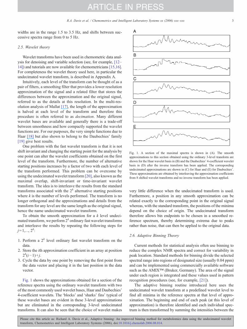
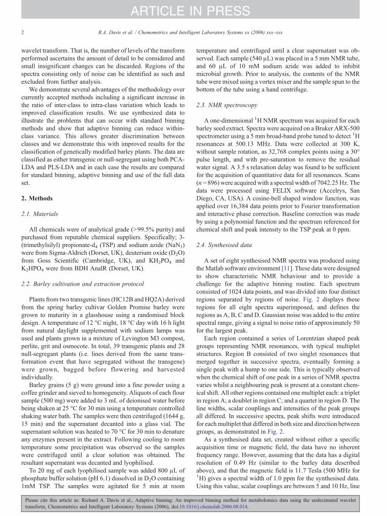
Fig. 1. A section of the maximal spectra is shown in (A). The smoothapproximations to this section obtained using the ordinary 3-level transform areshown for the Haar wavelet basis in (B) and the Daubechies' 4-coefficient waveletbasis in (D) after the inverse transform has been applied. The correspondingundecimated approximations are shown in (C) for Haar and (E) for Daubechies'.These approximations are obtained by interleaving the approximation coefficientsfrom 8 shifted wavelet transforms and no inverse transform has been applied.

3R.A. Davis et al. / Chemometrics and Intelligent Laboratory Systems xx (2006) xxx–xxx

ARTICLE IN PRESS

widths are in the range 1.5 to 3.5 Hz, and shifts between suc-cessive spectra range from 0 to 5 Hz.

2.5. Wavelet theory

Wavelet transforms have been used in chemometric data anal-ysis for denoising and variable selection (see, for example, [12–14]) and tutorials are now available for chemometricians [15,16].For completeness the wavelet theory used here, in particular theundecimated wavelet transform, is described in Appendix A.

Intuitively, each level of the transform can be thought of as apair of filters, a smoothing filter that provides a lower resolutionapproximation of the signal and a related filter that stores thedifferences between the approximation and the original signal,referred to as the details at this resolution. In the multi-res-olution analysis of Mallat [17], the length of the approximationis halved at each level of the transform and therefore thisprocedure is often referred to as decimation. Many differentwavelet bases are available and generally there is a trade-offbetween smoothness and how compactly supported the waveletfunctions are. For our purposes, the very simple functions due toHaar [18] but also shown to belong to the Daubechies' family[19] give best results.

One problem with the fast wavelet transform is that it is notshift invariant and changing the starting point for the analysis byone point can alter the wavelet coefficients obtained on the firstlevel of the transform. Furthermore, the number of alternativestarting positions increases by a factor of two with each level ofthe transform performed. This problem can be overcome byusing the undecimated wavelet transform [20], also known as themaximal overlap, shift-invariant or time-invariant wavelettransform. The idea is to interleave the results from the standardtransforms associated with the 2k alternative starting positionswhere k is the number of levels performed. The transform is nolonger orthogonal and the approximations and details from thetransform for any level are the same length as the original signal,hence the name undecimated wavelet transform.

To obtain the smooth approximation for a k level undeci-mated transform, we perform 2k ordinary fast wavelet transformsand interleave the results by repeating the following steps forj=1,…, 2k:

1. Perform a 2k level ordinary fast wavelet transform on thedata.

2. Store the ith approximation coefficient in an array at position2k(i−1)+ j.

3. Cycle the data by one point by removing the first point fromthe data vector and placing it in the last position in the datavector.

Fig. 1 shows the approximations obtained for a section of thereference spectra using the ordinary wavelet transform with twoof the most commonly used wavelet bases, Haar and Daubechies'4-coefficient wavelets. The ‘blocks’ and ‘sharks' fins’ typical ofthese wavelet bases are evident in these 3-level approximationsbut are eliminated in the corresponding 3-level undecimatedtransforms. It can also be seen that the choice of wavelet makes


very little difference when the undecimated transform is used.Furthermore, a position in any smooth approximation can berelated exactly to the corresponding point in the original signalwhereas, with the standard transform, the positions of the minimadepend on the choice of origin. The undecimated transformtherefore allows bin endpoints to be chosen in a smoothed re-ference spectrum, thereby determining extrema due to peaksrather than noise, that can then be applied to the original data.

2.6. Adaptive Binning Theory

Current methods for statistical analysis often use binning toreduce the complex NMR spectra and correct for variability inpeak location. Standard methods for binning divide the selectedspectral range into regions of designated size (usually 0.04 ppm)and can be implemented using commercially available softwaresuch as the AMIX™ (Bruker, Germany). The area of the signalunder each region is integrated and these values used in patternrecognition procedures (see, for example, [21]).

The adaptive binning routine introduced here uses theundecimated wavelet transform at a predefined wavelet level tofind all minima in the reference spectra at that level of appro-ximation. The beginning and end of each peak (at this level ofapproximation) is therefore identified and each individual spec-trum is then transformed by summing the intensities between the



https://www.researchgate.net/publication/267474212_Wavelet_Methods_for_Time_Series?el=1_x_8&enrichId=rgreq-5cc9ee739b7f4442c718f01fc04245b6-XXX&enrichSource=Y292ZXJQYWdlOzIyMjI3MjY1MjtBUzo5NzAyNjU5OTU1NTA4MEAxNDAwMTQ0MzUyNjg1

https://www.researchgate.net/publication/215659249_Ten_Lectures_On_Wavelets?el=1_x_8&enrichId=rgreq-5cc9ee739b7f4442c718f01fc04245b6-XXX&enrichSource=Y292ZXJQYWdlOzIyMjI3MjY1MjtBUzo5NzAyNjU5OTU1NTA4MEAxNDAwMTQ0MzUyNjg1

Fig. 2. The set of eight synthesised spectra. The insets (A), (C) and (D) show how the different samples are shifted in relation to each other for the triplet, doublet andquartet respectively. (B) shows that the second group consists of two separate peaks in some samples and one peak with a hump in others.


ARTICLE IN PRESS

minima. The reference spectrum must be chosen in such a waythat peaks occurring in any of the sample groups are accountedfor. Using the mean spectra over all groups, for example, couldaverage out peaks that occur in some samples but not others and itis precisely those peaks occurring in one class of samples but notanother that we want to determine. We have taken the maximum,over every sample to be used in the analysis, at each point in thespectra as our reference spectrum. Thus any peak occurring in anyindividual sample will be represented in the reference spectrum.

The wavelet transform has been widely used to reduce noisesince [22] first suggested the method. We use hard-thresholdingwith the threshold of r

ffiffiffiffiffiffiffiffiffiffiffiffiffi2logN

pto identify regions of noise in

the reference spectrum. Here N is the number of data points, σis the variance of the noise estimated by

r¼ medianfjw1;1j;…; jw1;N=2g0:6745


and w1,i represents the ith wavelet coefficient for the first levelof details. These noise regions represent null bins that areexcluded from further analyses.

The reference spectrum has a jagged appearance (see Fig. 1(A)) due to the peak shifts between samples and must besmoothed before its minima can be used to provide bin positions.This is achieved using the undecimated wavelet transform on thereference spectrum to a given number of wavelet levels. Theappropriate number of wavelet levels will depend on the res-olution of the raw data and is determined from the number ofdata points describing an average peak width (typically 1.5 Hz).Further details of the undecimated wavelet transform are givenin Appendix A but the basic idea is to interleave the smoothapproximations from the Fast Wavelet Transforms (FWTs)associated with the 2L alternative origins, where L is the numberof wavelet levels performed. The undecimated wavelet approx-imation, AL, obtained in this way is the same length as the




ARTICLE IN PRESS

original spectra and does not contain artifacts related to thechoice of wavelet filter.

The amount of smoothing is determined by the level, L, ofthe approximation and controls the number of minima detectedin the signal and therefore the number of peaks to be consideredseparately. At one level, small humps on peaks will be allocatedseparate bins but further smoothing (more levels of the trans-form) will combine bumps with the peak. A higher-level trans-form would potentially group together ranges of peaks.

We consider the point x in AL to be a minimum if both

ALðx−1Þ−ALðxÞN0 and ALðxþ 1Þ−ALðxÞN0:As the purpose of identifying minima is to locate the

beginning and end of each peak we include the points at eitherend of regions of noise, i.e. the points x such that

ALðx−1Þ ¼ 0 and ALðxÞN0 or ALðx−1ÞN0 and ALðxÞ ¼ 0:

This set of points {x1,…,xp} provide the start and end of eachbin and any bins consisting only of noise are ignored. For eachsample spectra the data are integrated over any valid bin and thesevalues used as the variables in subsequent statistical analyses.

The process may be summarized by applying the followingsteps to the reference spectrum:

(1) denoise(2) perform undecimated wavelet transform(3) find all minima(4) define non-noise bins.

The final step is to integrate the sample spectra over thesebins to create variables for classification.

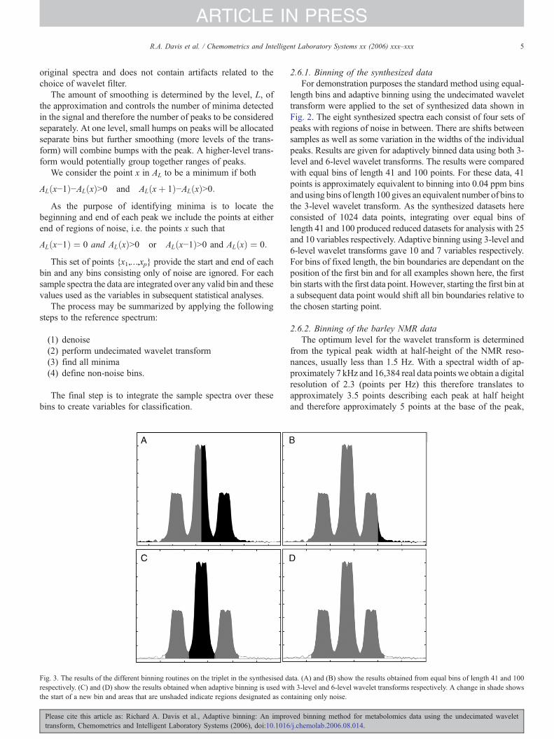
Fig. 3. The results of the different binning routines on the triplet in the synthesised drespectively. (C) and (D) show the results obtained when adaptive binning is used withe start of a new bin and areas that are unshaded indicate regions designated as co


2.6.1. Binning of the synthesized dataFor demonstration purposes the standard method using equal-

length bins and adaptive binning using the undecimated wavelettransform were applied to the set of synthesized data shown inFig. 2. The eight synthesized spectra each consist of four sets ofpeaks with regions of noise in between. There are shifts betweensamples as well as some variation in the widths of the individualpeaks. Results are given for adaptively binned data using both 3-level and 6-level wavelet transforms. The results were comparedwith equal bins of length 41 and 100 points. For these data, 41points is approximately equivalent to binning into 0.04 ppm binsand using bins of length 100 gives an equivalent number of bins tothe 3-level wavelet transform. As the synthesized datasets hereconsisted of 1024 data points, integrating over equal bins oflength 41 and 100 produced reduced datasets for analysis with 25and 10 variables respectively. Adaptive binning using 3-level and6-level wavelet transforms gave 10 and 7 variables respectively.For bins of fixed length, the bin boundaries are dependant on theposition of the first bin and for all examples shown here, the firstbin starts with the first data point. However, starting the first bin ata subsequent data point would shift all bin boundaries relative tothe chosen starting point.

2.6.2. Binning of the barley NMR dataThe optimum level for the wavelet transform is determined

from the typical peak width at half-height of the NMR reso-nances, usually less than 1.5 Hz. With a spectral width of ap-proximately 7 kHz and 16,384 real data points we obtain a digitalresolution of 2.3 (points per Hz) this therefore translates toapproximately 3.5 points describing each peak at half heightand therefore approximately 5 points at the base of the peak,

ata. (A) and (B) show the results obtained from equal bins of length 41 and 100th 3-level and 6-level wavelet transforms respectively. A change in shade showsntaining only noise.



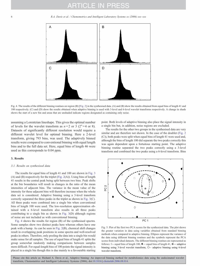
Fig. 4. The results of the different binning routines on region (B) [Fig. 2] in the synthesised data. (A) and (B) show the results obtained from equal bins of length 41 and100 respectively. (C) and (D) show the results obtained when adaptive binning is used with 3-level and 6-level wavelet transforms respectively. A change in shadeshows the start of a new bin and areas that are unshaded indicate regions designated as containing only noise.

Fig. 5. Plot of the first two PCA scores for the synthesized data. The plot showsthe greater variation in data using variables obtained from standard binningmethods when compared to adaptive binning. Ellipses represent the variance ofthe data using different binning routines and the symbols represent the PCAscores from individual datasets. The different binning routines are represented asfollows: ◊-- equal bins of length 100,♦― equal bins of length 41,●― adaptivebinning using 3-level wavelet transform, ○-- adaptive binning using 6-levelwavelet transform.


ARTICLE IN PRESS

assuming a Lorentzian lineshape. This gives the optimal numberof levels for the wavelet transform as n=2 or 3 (2n=4 or 8).Datasets of significantly different resolution would require adifferent wavelet level for optimal binning. Here a 2-leveltransform, giving 793 bins, was used. The adaptively binnedresults were compared to conventional binning with equal lengthbins and to the full data set. Here, equal bins of length 46 wereused as this corresponds to 0.04 ppm.

3. Results

3.1. Results on synthesised data

The results for equal bins of length 41 and 100 are shown in Fig. 3(A) and (B) respectively for the triplet (Fig. 2(A)). Using bins of length41 results in the central peak being split between two bins. Peak shiftsat the bin boundaries will result in changes in the ratio of the meanintensities of adjacent bins. The variance in the mean value of theintensity for these adjacent bins will therefore increase when the wholedata set is considered. Adaptive binning using a 3-level transformcorrectly separated the three peaks in the triplet as shown in Fig. 3(C).All three peaks were combined into a single bin when conventionalbins of length 100 were used. The low-resolution approximation ob-tained with a 6-level transform also results in all three peakscontributing to a single bin as shown in Fig. 3(D) although regionsof noise are not included as with conventional binning.

Fig. 4 shows the results for region (B) of the synthesised spectra.Some samples show two distinct peaks here whereas others have onepeak with a hump. As can be seen in Fig. 2(B), chemical shift changesresult in overlapping peak positions in some spectra and well-resolvedpeaks in others. Therefore, only pooling the data into a single bin wouldmake sense for all samples. The use of equal bins of length 41 splits thegroup somewhat randomly making comparisons between samplesmore difficult. For equal-length bins of 100 points the signal intensity isplaced in a single bin though this is due mainly to a favourable starting


point. Both levels of adaptive binning also place the signal intensity ina single bin but, in addition, noise regions are excluded.

The results for the other two groups in the synthesised data are verysimilar and are therefore not shown. In the case of the doublet (Fig. 2(C)), both peaks were split when equal bins of length 41 were used and,although the bins of length 100 did separate the two peaks correctly thiswas again dependent upon a fortuitous starting point. The adaptivebinning routine separated the two peaks correctly using a 3-leveltransform and combined the two peaks using a 6-level transform. Bins



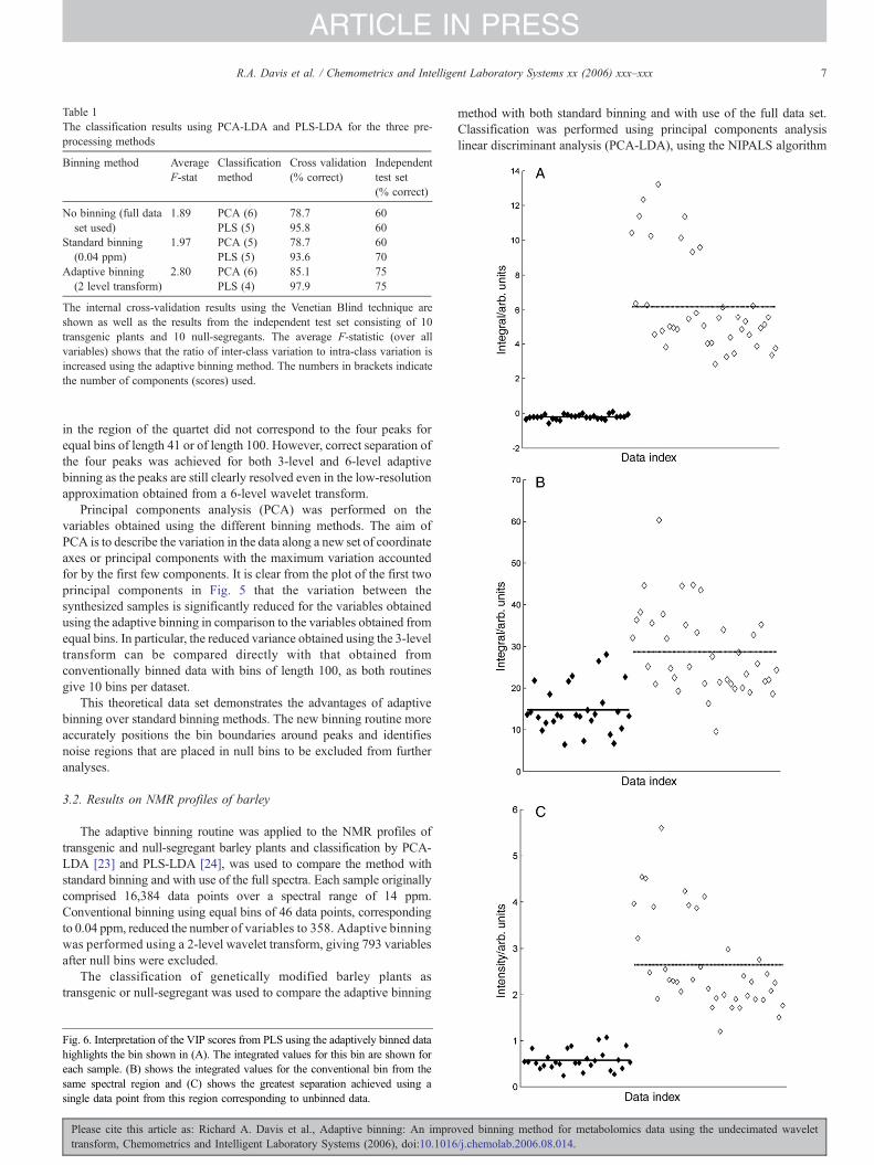
Table 1The classification results using PCA-LDA and PLS-LDA for the three pre-processing methods

Binning method AverageF-stat

Classificationmethod

Cross validation(% correct)

Independenttest set(% correct)

No binning (full dataset used)

1.89 PCA (6) 78.7 60PLS (5) 95.8 60

Standard binning(0.04 ppm)

1.97 PCA (5) 78.7 60PLS (5) 93.6 70

Adaptive binning(2 level transform)

2.80 PCA (6) 85.1 75PLS (4) 97.9 75

The internal cross-validation results using the Venetian Blind technique areshown as well as the results from the independent test set consisting of 10transgenic plants and 10 null-segregants. The average F-statistic (over allvariables) shows that the ratio of inter-class variation to intra-class variation isincreased using the adaptive binning method. The numbers in brackets indicatethe number of components (scores) used.


ARTICLE IN PRESS

in the region of the quartet did not correspond to the four peaks forequal bins of length 41 or of length 100. However, correct separation ofthe four peaks was achieved for both 3-level and 6-level adaptivebinning as the peaks are still clearly resolved even in the low-resolutionapproximation obtained from a 6-level wavelet transform.

Principal components analysis (PCA) was performed on thevariables obtained using the different binning methods. The aim ofPCA is to describe the variation in the data along a new set of coordinateaxes or principal components with the maximum variation accountedfor by the first few components. It is clear from the plot of the first twoprincipal components in Fig. 5 that the variation between thesynthesized samples is significantly reduced for the variables obtainedusing the adaptive binning in comparison to the variables obtained fromequal bins. In particular, the reduced variance obtained using the 3-leveltransform can be compared directly with that obtained fromconventionally binned data with bins of length 100, as both routinesgive 10 bins per dataset.

This theoretical data set demonstrates the advantages of adaptivebinning over standard binning methods. The new binning routine moreaccurately positions the bin boundaries around peaks and identifiesnoise regions that are placed in null bins to be excluded from furtheranalyses.

3.2. Results on NMR profiles of barley

The adaptive binning routine was applied to the NMR profiles oftransgenic and null-segregant barley plants and classification by PCA-LDA [23] and PLS-LDA [24], was used to compare the method withstandard binning and with use of the full spectra. Each sample originallycomprised 16,384 data points over a spectral range of 14 ppm.Conventional binning using equal bins of 46 data points, correspondingto 0.04 ppm, reduced the number of variables to 358. Adaptive binningwas performed using a 2-level wavelet transform, giving 793 variablesafter null bins were excluded.

The classification of genetically modified barley plants astransgenic or null-segregant was used to compare the adaptive binning

Fig. 6. Interpretation of the VIP scores from PLS using the adaptively binned datahighlights the bin shown in (A). The integrated values for this bin are shown foreach sample. (B) shows the integrated values for the conventional bin from thesame spectral region and (C) shows the greatest separation achieved using asingle data point from this region corresponding to unbinned data.


method with both standard binning and with use of the full data set.Classification was performed using principal components analysislinear discriminant analysis (PCA-LDA), using the NIPALS algorithm



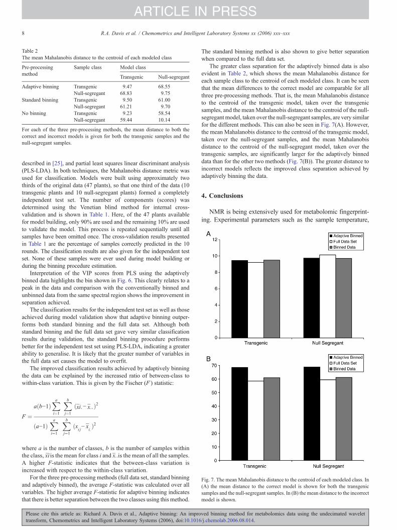
Table 2The mean Mahalanobis distance to the centroid of each modeled class

Pre-processingmethod

Sample class Model class

Transgenic Null-segregant

Adaptive binning Transgenic 9.47 68.55Null-segregant 68.83 9.75

Standard binning Transgenic 9.50 61.00Null-segregant 61.21 9.70

No binning Transgenic 9.23 58.54Null-segregant 59.44 10.14

For each of the three pre-processing methods, the mean distance to both thecorrect and incorrect models is given for both the transgenic samples and thenull-segregant samples.

Fig. 7. The mean Mahalanobis distance to the centroid of each modeled class. In(A) the mean distance to the correct model is shown for both the transgenicsamples and the null-segregant samples. In (B) the mean distance to the incorrectmodel is shown.


ARTICLE IN PRESS

described in [25], and partial least squares linear discriminant analysis(PLS-LDA). In both techniques, the Mahalanobis distance metric wasused for classification. Models were built using approximately twothirds of the original data (47 plants), so that one third of the data (10transgenic plants and 10 null-segregant plants) formed a completelyindependent test set. The number of components (scores) wasdetermined using the Venetian blind method for internal cross-validation and is shown in Table 1. Here, of the 47 plants availablefor model building, only 90% are used and the remaining 10% are usedto validate the model. This process is repeated sequentially until allsamples have been omitted once. The cross-validation results presentedin Table 1 are the percentage of samples correctly predicted in the 10rounds. The classification results are also given for the independent testset. None of these samples were ever used during model building orduring the binning procedure estimation.

Interpretation of the VIP scores from PLS using the adaptivelybinned data highlights the bin shown in Fig. 6. This clearly relates to apeak in the data and comparison with the conventionally binned andunbinned data from the same spectral region shows the improvement inseparation achieved.

The classification results for the independent test set as well as thoseachieved during model validation show that adaptive binning outper-forms both standard binning and the full data set. Although bothstandard binning and the full data set gave very similar classificationresults during validation, the standard binning procedure performsbetter for the independent test set using PLS-LDA, indicating a greaterability to generalise. It is likely that the greater number of variables inthe full data set causes the model to overfit.

The improved classification results achieved by adaptively binningthe data can be explained by the increased ratio of between-class towithin-class variation. This is given by the Fischer (F ) statistic:

F ¼aðb−1Þ

Xai¼1

Xbj¼1

ðxi:− x::Þ2

ða−1ÞXai¼1

Xbj¼1

ðxi j− x

i:Þ2

where a is the number of classes, b is the number of samples withinthe class, xi is the mean for class i and x..¯ is the mean of all the samples.A higher F-statistic indicates that the between-class variation isincreased with respect to the within-class variation.

For the three pre-processing methods (full data set, standard binningand adaptively binned), the average F-statistic was calculated over allvariables. The higher average F-statistic for adaptive binning indicatesthat there is better separation between the two classes using this method.


The standard binning method is also shown to give better separationwhen compared to the full data set.

The greater class separation for the adaptively binned data is alsoevident in Table 2, which shows the mean Mahalanobis distance foreach sample class to the centroid of each modeled class. It can be seenthat the mean differences to the correct model are comparable for allthree pre-processing methods. That is, the mean Mahalanobis distanceto the centroid of the transgenic model, taken over the transgenicsamples, and the mean Mahalanobis distance to the centroid of the null-segregant model, taken over the null-segregant samples, are very similarfor the different methods. This can also be seen in Fig. 7(A). However,the mean Mahalanobis distance to the centroid of the transgenic model,taken over the null-segregant samples, and the mean Mahalanobisdistance to the centroid of the null-segregant model, taken over thetransgenic samples, are significantly larger for the adaptively binneddata than for the other two methods (Fig. 7(B)). The greater distance toincorrect models reflects the improved class separation achieved byadaptively binning the data.

4. Conclusions

NMR is being extensively used for metabolomic fingerprint-ing. Experimental parameters such as the sample temperature,




ARTICLE IN PRESS

pH and ionic strength at which NMR spectra are recorded, leadto changes in the dynamics of the sample and therefore peakpositions. Such spectral changes must be accounted forwhen comparing samples in metabolomic studies and databinning is a widely accepted method for dealing with peakshifts. Integration over regions of equal length with an arbi-trary starting point can in fact introduce additional intra-class variation, assigning shifted peaks to different bins andtherefore exacerbating the very problem it was designed toovercome.

The adaptive binning described here overcomes the problemsassociated with the currently accepted method of binning. Thereference spectrum, in which each data point is the maximumover all spectra for that point, allows each peak in everyspectrum to be considered. The wavelet transform then smoothesthis reference spectrum, so that peaks shifted between spectra arecombined into a single peak. The bin boundaries are then placedon either side of the reference peak ensuring that the bins aredirectly related to the peaks in this spectrum and that peaks arenot split between bins. Peaks can be considered individually or,with further smoothing, combined in a single bin. This facilitatesinterpretation of the results by relating peaks or spectral ranges toindividual metabolites. The amount of smoothing depends onthe number of levels of the wavelet transform and can beadjusted according to the data resolution and the shifts expectedbetween samples. More levels of the transform may therefore berequired to deal with variable matrices, such as urine, as theseoften display larger chemical shifts, which translate to broaderpeaks in the reference spectrum.

The adaptive binning method also has advantages for patternrecognition procedures in comparison to use of the full data set.In a recent study [6] it was found that class separation was basedonly on chemical shifts between two classes. One particular peakwas shifted in such a way that, for all samples in one class, themaximum intensity of the peak was being compared to the tail ofthe peak in all samples of the other class. This overoptimisticseparation did not represent the true distinction between theclasses whereas the adaptive binning method provided a morerealistic classification by integrating over the whole peak rangefor both classes.

The adaptive binning method has been compared to thestandard method using bins of equal length on both syn-thesized and real data sets. A significant reduction in the intra-class variation was found using adaptive binning. The standardmethod of binning to 0.04 ppm has been found to give signif-icantly fewer bins than the number of peaks in the spectra. Byminimising intra-class variation using adaptive binning, inter-class variation is more easily detected using, for example,genetic programming [26]. Furthermore, as the bins are relatedto actual peaks in the spectra with noise regions excluded,relevant differences between sample groups are more easilyinterpreted. The chemical shift ranges that are determined asthe bin boundaries by adaptive binning can be specificallyrelated to molecular characteristics. Thus, bins found to dis-criminate classes can be related to chemical structure usingNMR databases and 2-D NMR methods, facilitating com-pound identification.


Acknowledgements

We thank the Engineering and Physical Sciences ResearchCouncil (EPSRC) and the Department for Environment, Foodand Rural Affairs (DEFRA) for supporting RAD.

JCW is a Royal Society University Research Fellow. Wethank Dr. W. Harwood (John Innes Centre, Norwich, UK) forprovision of the barley samples and staff in the NMR section atthe Central Science Laboratory for the NMR data. The contri-bution of both JIC and CSL was funded by the UK FoodsStandards Agency.

Appendix A. Wavelet theory

In Fourier analysis the basis functions are sines and cosinesand each contributes to the entire signal. Thus, whilst theFourier transform provides information about the differentfrequencies present in a signal, it can give no information aboutwhere in the signal these frequencies occur. The wavelettransform on the other hand uses basis functions, or wavelets,that are localised in both position (or time) and frequency. In themulti-resolution analysis of Mallat [17] the signal, f (x), isinitially expressed in terms of the translates of a scaling func-tion, φ. Defining

uj;k xð Þ ¼ ux2 j

−k� �

;

so that j and k determine the scale and position respectively, wehave

f ðxÞ ¼XN−1

k¼0

h f ;u0;kiu0;kðxÞ

where ⟨ f,φj,k⟩ is the inner product of the signal with the waveletfunction φj,k (x). The function, φ, is chosen so that rescaling bya factor of 2 gives the lower resolution approximation

f ðxÞcXðN−1Þ=2

k¼0

h f ;u1;kiu1;kðxÞ

in which the coefficients, ⟨ f,φ1,k⟩, can be obtained from thecoefficients, ⟨ f,φ0,k⟩. The relationship between the coefficientsis obtained via a scaling equation relating the functions φj,k (x)at level j to the functions φj−1,k (x) at level j−1. The differencesbetween the approximation and the original signal areexpressed in terms of a related wavelet function, ψ, so thatthe signal may also be expressed exactly as

f ðxÞ ¼XðN−1Þ=2

k¼0

h f ;u1;kiu1;kðxÞ þXðN−1Þ=2

k¼0

h f ;w1;kiw1;kðxÞ





ARTICLE IN PRESS

where the coefficients ⟨ f,ψ1,k⟩ can also be calculated from thecoefficients,⟨ f,ψ0,k⟩. The relationship between the waveletcoefficients on one level and those on the previous level allowsthe discrete wavelet transform to be implemented in fastalgorithms using matrix methods.

The scaling function, ϕ, can be thought of as a low-passfilter retaining the low frequency information as an approxi-mation to the signal. The wavelet function, ψ, behaves as ahigh-pass filter, collecting the high frequency information ordetails in the signal. One application of these two filters, a singlelevel of the wavelet transform, on a signal of length 2 j results intwo signals each of length 2 j−1 referred to as the approximationsand details. The procedure can be repeated on the approxima-tion of the signal at each successive level of the transform. Ateach level the length of the approximation is halved and there-fore this procedure is often referred to as decimation. However,at each level the details are encoded by the wavelet functionsand no information is lost. At any stage the original signal canbe recovered using the inverse wavelet transform in which therelevant details are recombined with the approximation of thesignal.

However the fast wavelet transform is not shift invariant.Although it is possible to calculate 2 j separate inner products,⟨f,φ1,k⟩, and a further 2 j inner products,⟨ f,ψ1,k⟩, from a signalof length 2 j, the down-sampling inherent in the fast wavelettransform means that only 2 j−1 approximation coefficients, ⟨f,φ1,k⟩, and 2 j−1 detail coefficients,⟨ f,ψ1,k⟩, need to be com-puted. In fact only every second possible inner product isnecessary in order to represent the signal exactly. For example,the Haar approximation coefficients involve the average of thefirst and second points in the signal, the average of the third andfourth and so on but the average of the second and third points,for example, is not considered. Similarly the related detailcoefficients do not involve the difference between the secondand third points, the fourth and fifth points, etc. Thus changingthe starting point for the analysis by one point can alter thewavelet coefficients obtained on the first level of the transform.Furthermore, the number of alternative starting positions in-creases by a factor of two with each level of the transformperformed. On the second level, for example, the Haarcoefficients will involve groups of four points so that startingthe transform at the first, second, third or fourth points in thesignal will produce different sets of second level waveletcoefficients. However, starting at the fifth point would producethe same set of coefficients as starting at the first point but withone coefficient (the first) missing. To illustrate this, we intro-duce the notation

Wsl;mðp1;…; p2lÞ

for an approximation coefficient, W, where s denotes thestarting point of the transform, l the level, m the coefficientnumber and p1,…,p2l indicate the data points involved. Then

Vsl;mðp1;…; p2lÞ


represents the corresponding detail coefficient. One level of thetransform, starting from point one will then produce the set of n

2approximation coefficients

W 11;1 1; 2ð Þ;W 1

1;2 3; 4ð Þ;…;W 11;n2

n−1; nð Þn o

whereas, starting from point two will yield

W 21;1 2; 3ð Þ;W 2

1;2 4; 5ð Þ;…;W 11;n2

n; 1ð Þn o

with corresponding sets of detail coefficients. Here n is thenumber of data points in the signal. Notice that the last coef-ficient, when stating at point two, involves the first point of thesignal as the transform assumes periodicity of the signal.Although starting from point three will produced the same firstlevel coefficients as starting from point one (cycled by one),these two starting points will give different second levelcoefficients. The second level of the transform will replace thelevel-one approximation coefficients with

W 12;1 1; 2; 3; 4ð Þ;W 1

2;2 5; 6; 7; 8ð Þ;…;W 12;n4

n−3; n−2; n−1; nð Þn o

;

W 22;1 2; 3; 4; 5ð Þ;W 2

2;2 6; 7; 8; 9ð Þ;…;W 22;n4

n−2; n−1; n; 1ð Þn o

;

W 32;1 3; 4; 5; 6ð Þ;W 3

2;2 7; 8; 9; 10ð Þ;…;W 32;n4

n−1; n; 1; 2ð Þn o

or

W 42;1 4; 5; 6; 7ð Þ;W 4

2;2 8; 9; 10; 11ð Þ;…;W 42;n4

n; 1; 2; 3ð Þn o

for starting points one, two, three and four respectively withcorresponding sets of n

4 detail coefficients. Although we haveused the Haar wavelet basis, the problem is the same for anywavelet family. The shift in the data points involved will alwaysbe a power of two but the actual number of points involved inthe calculation of a coefficient will depend on the support of thewavelet.

The problem of shift invariance can be overcome by amethodknown as cycle spinning [27] in which the transform is applied toevery cycle of the signal and the average taken for each point.However, this method is time consuming and computationallyexpensive. A simpler method is to apply the undecimatedwavelet transform [20]. Unlike cycle-spinning, in which everypossible cycle (i.e. one transform for every point in the originalsignal) is computed, the undecimated wavelet transform onlyrequires the transforms associated with the 2k alternative startingpositions (where k is the number of levels of the transform to beperformed). Implementation can vary but the idea is always tointerleave the results from these 2k standard transforms of thesignal (or previous approximation of it). For example, the twosets of first level approximation coefficients above are inter-leaved to give the n coefficients:

W 11;1 1; 2ð Þ;W 2

1;1 2; 3ð Þ;W 11;2 3; 4ð Þ;W 2

1;2 4; 5ð Þ;…;W 11;n2

n−1; nð Þ;W 21;n2

n; 1ð Þn o

:

Similarly, the approximation coefficients from each subse-quent level are interleaved, as are the detail coefficients. The




ARTICLE IN PRESS

resulting transform is no longer orthogonal and the approxima-tions and details from the transform for any level are the samelength as the original signal, hence the name undecimatedwavelet transform.

References

[1] L.W. Sumner, P. Medes, R.A. Dixon, Phytochemistry 62 (2003) 817–836.[2] M.E. Bollard, E.G. Stanley, J.C. Lindon, J.K. Nicholson, E. Holmes, NMR

Biomed. 18 (2005) 143–162.[3] A.J. Charlton, A.L. Davis, D.P. Jones, J.R. Lewis, A.P. Davies, E. Haslam,

M.P. Willeamson, J. Chem. Soc., Perkin Trans., 2 2 (2000) 317–322.[4] J. Forshed, I. Schuppe-Koistinen, S.P. Jacobsson, Anal. Chim. Acta 487

(2003) 189–199.[5] A.J. Charlton, W.H. Farrington, P. Brereton, J. Agric. Food Chem. 50

(2002) 3098–3103.[6] A. Charlton, T. Allnutt, S. Holmes, J. Chisholm, S. Bean, N. Ellis, P.

Mullineaux, S. Oehlschlager, Plant Biotech. J. 2 (2004) 27–35.[7] J.L. Griffin, H.J. Williams, E. Sang, K. Clarke, C. Rae, J.K. Nicholson,

Anal. Biochem. 293 (2001) 16–21.[8] O. Beckonert, M.E. Bollard, T.M.D. Ebbels, H.C. Keun, H. Antii, E.

Holmes, J.C. Lindon, J.K. Nicholson, Anal. Chim. Acta 490 (2003) 3–15.[9] Matlab, The MathWorks Inc., Natick, MA, USA. (2002).[10] B. Walczak, D.L. Massart, Chemometr. Intell. Lab. Syst. 36 (1997) 81–94.[11] B.K. Alsberg, A.M. Woodward, M.K. Winson, J.J. Rowland, D.B. Kell,

Anal. Chim. Acta 368 (1998) 29–44.


[12] C. Perrin, B. Walczak, D.L. Massart, Anal. Chem. 73 (2001) 4903–4917.[13] B.K. Alsberg, A.M. Woodward, D.B. Kell, Chemometr. Intell. Lab. Syst.

37 (1997) 215–239.[14] K. Krzsztof, B. Walczak, S. de Jong, G.M. Vandeginste, Proteomics 4

(2004) 2377–2389.[15] S. Mallat, IEEE Trans. Pattern Anal. Mach. Intell. 11 (7) (1989) 674–693.[16] A. Haar, Math. Ann. 69 (1910) 331–371.[17] Daubechies, I. Ten Lectures on Wavelets, CMBS-NSF Reg. Conf. Series in

Applied Math. SIAM.[18] D.B. Percival, A.T. Walden, Wavelet Methods for Time Series Analysis,

Cambridge University Press, Cambridge, 2000.[19] M.A. Warne, E.M. Lenz, D. Osborn, J.M. Weeks, J.K. Nicholson, Soil

Biochem. 33 (2001) 1171–1180.[20] D.L. Donoho, I.M. Johnstone, Biometrika 81 (1994) 425–455.[21] H. Wold, in: P.R. Krishnaiah (Ed.), Multivariate Analysis, Academic Press,

1966, pp. 391–420.[22] S. Wold, Chemometr. Intell. Lab. Syst. 14 (1992) (1992) 71–84.[23] B.G.M. Vandeginste, D.L. Massart, L.M.C. Buydens, S. De Jong, P.J.

Lewi, J. Smeyers-Verbeke, Handbook of Chemometrics and Qualimetrics:Part B, Elsevier, 1997.

[24] Davis, R.A., Charlton, A.J., Oehlschlager, S., Wilson, J. (2005). Chemom.Intell. Lab. Syst. 81 (1) (2006) 50−59.

[25] R.R. Coifman, D.L. Donoho, Wavelets and Statistics, in: A. Antoniadis, G.Oppenheim (Eds.), Lecture Notes in Statistics, vol. 103, Springer Verlag,New York, 1995, pp. 125–150.







Adaptive binning: An improved binning method for metabolomics data using the undecimated wavelet...

Documents

Transcript of Adaptive binning: An improved binning method for metabolomics data using the undecimated wavelet...