Submitted to: IEEE Transactions on Image Processing, April 1998, Revised:June 1999Fast Adaptive Wavelet Packet Image Compression

Francois G. Meyer, Yale University, New Haven, USA

Amir Averbuch, Tel Aviv University, Tel Aviv, Israel

Jan-Olov Stromberg, Royal Institute of Technology, Stockholm, Sweden

Corresponding author:

Francois G. Meyer

Yale University School of Medicine, Department of Diagnostic Radiology

333 Cedar Street, P.O. Box 208042, New Haven, CT 06520-8042, USA

tel:(203) 737 6037, fax:(203) 737 4273, e-mail: francois.meyer@yale.eduEDICS Category: IP 1.1 Coding

Abstract

Wavelets are ill suited to represent oscillatory patterns: rapid variations of intensity can only

be described by the small scale wavelet coefficients. These diffused coefficients carry very little

energy, and are often quantized to zero, even at high bit rates. Our goal in this paper is to provide

a fast numerical implementation of the best wavelet packet algorithm [8] in order to demonstrate

that an advantage can be gained by constructing a basis adapted to a target image. Emphasis

in this paper has been placed on developing algorithms that are computationally efficient. We

developed a new fast 2-D convolution-decimation algorithm with factorized non-separable 2-D

filters. The algorithm is 4 times faster than a standard convolution-decimation. An extensive

evaluation of the algorithm was performed on a large class of textured images. Because of its

ability to reproduce textures so well, the wavelet packet coder significantly outperforms one of

the best wavelet coder [26] on images such as Barbara, and Fingerprints, both visually and in term

of PSNR.

1 Introduction

The main defect of the windowed Fourier based compression methods (such as the DCT) is due to

the limitation put on the size of the blocks, and the inability to adjust the patterns to the nature of the

picture. An answer to this problem is provided by a multiscale decomposition of the image: - low

frequency trends occurring at a large scale in the image can be efficiently coded with very few coef-

ficients. Wavelets with many vanishing moments yield sparse decompositions of piece-wise smooth

surfaces, and are very effective for coding piece-wise smooth images [1, 14, 26, 28, 30]. Wavelets,

however, are ill suited to represent oscillatory patterns. Rapid variations of intensity can only be de-

scribed by the small scale wavelet coefficients. Long oscillatory patterns thus require many of such

fine scale coefficients. Unfortunately, those small scale coefficients carry very little energy, and are

often quantized to zero, even at high bit rates. Much larger libraries of functions, called wavelet

packets, have been constructed [7] to address this problem. The wavelet packets include wavelets, as

well as cosine-like waveforms. In the the two dimensional (2-D) case, wavelet packets are patterns

that can vary in scale, frequency, and location. Because the collection of wavelet packets is over-

complete (there are many more basis functions than the dimension of the input space) one can now

construct a basis that is fitted for a target image (or for a class of images). In general a basis is a good

basis if it can describe the target image with a very small number of basis vectors. In their original

paper Coifman and Wickerhauser proposed a very generic metric to assess the efficiency of a basis

[8]. A more meaningful measure considers the number of bits needed to approximate the image with

a given error. Ramchandran and Vetterli [24] followed this path, and wedded the bit allocation algo-

rithm of Shoham and Gersho [29] to the best basis algorithm [8]. Unfortunately this approach (and

its variation [34]) is extremely computationally intensive (as explained in Section 4.2 the problem in

[24] involves 3 layers of non linear approximations, only one of which lends itself to a fast algorithm).

Very little work has been expended beyond the papers [8, 24], and as a result adapted wavelet packet

bases remain a theoretical curiosity, with no clear practical advantage, and that cannot be computed

within a reasonable amount of time.

Our goal in this paper is to provide a fast numerical implementation of the best wavelet packet

algorithm, in order to demonstrate that an advantage can be gained by constructing a basis adapted

to a target image. Many classes of images, or multidimensional signals, have very diffuse represen-

tations in a standard wavelet basis. Fingerprints, or seismic signals are few examples of non wavelet-

friendly signals. An adapted wavelet packet basis can often provide a very sparse representation

of such images. Fast algorithms for choosing a best basis are therefore of fundamental importance.

2

Emphasis in this paper has been placed on developing algorithms that are computationally efficient.

Three original contributions result from this work:

1. A new fast 2-D convolution-decimation algorithm with factorized non-separable 2-D filters.

The number of operations is reduced by a factor 4 in comparison to a standard implementation,

and the transform is performed in place (no transpose).

2. A cost function that takes into account the cost of coding the output levels of the quantizers,

and the cost of coding the significance map.

3. A context-based entropy coder that conditions the probability of significance of a given pixel

on the probability of its neighbors using a space filling curve.

This paper is organized as follows. In the next section we provide a general description of the prin-

ciples of the algorithm. In section 3 we review the wavelet packet library. In section 4 we explain

how to select, among a large collection of bases, that basis which is best adapted to encode a given

image. The factorization of the conjugate quadrature (lowpass and highpass) filters is described in

section 5. In section 6 we describe the quantization, and the context-based entropy coding. Results

of experiments are presented in Section 7.

Best basis

libraries of bases

Collection of

original

image expansion

Description of the best basis

1

bit stream

budget

2 3

Quantization

entropycoding

entropycoding

Figure 1: Block diagram of the wavelet packet compression algorithm. The compression consists of three

parts: (1) best basis selection, and calculation of the coefficients of the image, (2) quantization of the coefficients,

and (3) entropy coding. The quadtree that describes the best basis is also entropy coded.

2 General description of the compression algorithm

A block diagram of the algorithm is shown in Fig. 1. The algorithm is divided into three parts.

In the first part (1) we select that wavelet packet basis which is best adapted to encode the image.

During the second part (2), the wavelet packet coefficients of the image are quantized ; we assume

3

a Laplacian distribution and we use an efficient near optimal scalar quantizer [31]. Finally in (3),

the significance map, and the output levels are entropy coded. We exploit a higher order arithmetic

coder that relies on a context consisting of pixels in the causal neighborhood.

3 The wavelet packet library

The wavelet packet library [7] is composed of functions, with different time frequency localizations,

that provide a highly redundant representation: - there is not a unique decomposition of each image

over the library. Let fhng;fgng be biorthogonal filters, and let fhng;fgng be the dual filters ; fhng,fhng are the lowpass filters, and the conjugate quadrature filter sequences are:gn = (�1)n h1�n gn = (�1)n h1�n (1)

Let x be a discrete signal x= fxng ; n= 0; : : : , N� 1, thewavelet packet coefficientswn; j; l are definedby the following recursion:

w2n; j;l =∑k

gk�2l wn; j+1;k l = 0; : : : ;N 2 j�J (2)

w2n+1; j;l =∑k

hk�2l wn; j+1;k l = 0; : : : ;N 2 j�J (3)

w0;J;l = xl l = 0; : : : ;N (4)

The indices are interpreted as follows:� j is the scale index: the size of the support of the corresponding wavelet packet is 2� j. Thesignal x is sampled at the finest scale J: the distance between two samples is 2�J.� l is the localization parameter: the corresponding wavelet packet is located at l 2� j,� n is the frequency index: the wavelet packet has roughly n oscillations (a frequency 2 j n).

As shown in Fig. 2 the library organizes itself into a binary tree, where the nodes of the tree represent

subspaces with different time-frequency localization characteristics. The standard dyadic wavelet

basis is obtained by iterating the decomposition process on the low frequency bands only, without

further decomposing the high frequency component at each level of the tree.

4

sd1 dd1

d1

sd2

ddssdsdsssss

ds2

d2s4s3s2 d3

ds1ss2ss1

d4

ssd

G G

GH

H H H HG

dd2

dddsdddsd

H

G

GH

G

s1

x1 x2 x3 x4 x8x7x6x5

Figure 2: Wavelet packet tree. At each node of the tree, we apply a convolution and a decimation with the

lowpass filter H, and the highpass filter, G. The prefix “s” stands for the sum, or lowpass filter, and “d” stands

for difference or highpass filter.

3.1 Arbitrary image size, and boundary extension

In order to apply the lowpass and highpass filters to a sequence of arbitrary finite lengthN, we extend

the sequence on both end points of the sequence. Because we are using odd filters we extend the

sequence symmetrically [4]. This approach does not introduce any discontinuity at the boundaries.

When the number of samples in the sequence is odd,N= 2n+1, we obtain n+1 lowpass coefficients:sjkk = 0; : : : ;n , and n highpass coefficients: d j

kk = 0; : : : ;n� 1, as shown in Fig. 3.

s1 d

1

2n-3x

2n-1x

2n-2x

2n -1x

2nxx

1

s0 d

0

2x

2x

1x

0x

n-1s

n-1d

ns

Figure 3: 1-D periodic even extension. N = 2n+ 1. (s = lowpass, d = highpass).x

2n-3x

2n-2x

d1 n-1 n-1

ds1

2n -1x

2n-2x

2n-3

s

2x

1

s0 d

xx2

x1

x0

0

Figure 4: 1-D periodic even extension. N = 2n. (s = lowpass, d = highpass).4 Best basis algorithm

Clearly the library provides an overcomplete description of the signal x. We need to know how to

assemble the elements of the library to obtain an orthogonal basis. Loosely speaking, wavelet packets

make it possible to adaptively tile the frequency domain into different bands of arbitrary size ; if a

5

collection of functions in the library provides a cover of the time-frequency plane, then this set of

functions is an orthonormal basis. If we associate the dyadic frequency interval [2 jn; 2 j(n+ 1) ) to thewavelet packet coefficient wn; j; l, then we can build orthonormal bases from the binary tree [7]:Theorem 1 [7] If a subset E � N �Z has the property that the union of intervals

[2 jn; 2 j(n+ 1) ); j 2 N; 0 � n < 2 j; (n; j) 2 Eis a disjoint cover of [0;1), then the set of wavelet packet coefficients wn; j; l, with (n; j)2 E, are the coefficientsof x in an orthonormal basis.

The greater flexibility offered by the redundancy of the wavelet packet library can be exploited to

increase the efficiency of the representation. For each target image, we select from the library a basis

that is better fitted for the compression of that image.

4.1 A fast dynamic programming approach

From the previous theorem we learn that we have an extremely large amount of freedom for the

construction of orthogonal basis from the wavelet packets library. In fact, if we consider only dyadic

subdivision at each level, we still get 24Lbases for L levels. An exhaustive search inside the library

is absolutely impossible: for 6 levels there exist 24096 � 101200 bases ! In the case of wavelet packetsconstructed by dyadic subdivision, Coifman and Wickerhauser [8] suggested to use a fast dynamic

programming algorithm (order N log(N), where N is the number of pixels in the image) to search for

that best basis which is optimal according to a given cost function. A key criterion must be met in

order to invoke a dynamic programming strategy [9]: the objective function should be separable. In

the context of the best basis algorithm, this condition states that one must limit oneself to additive

cost-function [32]. Let x be a vector in one of the subspace defined by the wavelet packet tree, let

B = f'kg be any basis of that subspace, M is an additive cost function if there exists a positive

function � such that [32] : � (0) = 0 and M (x) =∑k

� (xk) (5)

where xk =<x; 'k>.4.2 Choice of a cost function

The metric defined by the objective function defines the optimality criterion. In this work, one basis

is better than another if it provides a better reconstruction quality for the same number of bits spent

6

in coding the coefficients, or if it requires less bits to achieve the same reconstruction quality. Initially

Coifman and Wickerhauser [8] proposed to use the entropy of the vector x :

h(x) = �∑k

jxkj2kxk2 log jxkj2kxk2 (6)

as a cost function. As is obvious h is not an additive cost function, however�h(x)� logkxk2�kxk2 is

an additive cost function, and minimizing the latter function over a set of basis that preserve kxk2will minimize (6). It is important to realize that (6) bears no connection with the entropy H (x) of

the probability distribution of the fxkg. For instance, if all xk are equal, then h(x) is maximal, but theentropy of the distribution H (x) is minimal. In practice, we have noticed that the cost function (6) is

usually of little value because it fails to discover any meaningful bases. Because h(x) is not related to

the theoretical number of bits required to code the coefficients <x; 'k>, Ramchandran and Vetterli[24] used the optimal bit allocation algorithm of Shoham and Gersho [29] to select the best basis B

according to the rate distortion criterion:

M (x;Q; �)= D(x;Q)+ �R(x;Q) (7)

Given a set of quantizers Q, the rate R(x;Q) is estimated with the first order approximation of theentropyH (Q(x)), and the distortion R(x;Q) is defined as the mean square error: 1Np∑k(xk �Q(xk))2.The selection of the best basis is part of an embedded optimization problem that involves three non-

linear optimization:

max� (minB2B ( ∑

node2B minQ2Q f D(x;Q)+ �R(x;Q)g)) (8)

Each node of the wavelet packet tree is associated with the best scalar quantizer Q for that node

using an exhaustive search among a predefined set Q of scalar quantizers. Then the best basis B

is obtained using the fast dynamic programming algorithm described above. Unfortunately the dy-

namic programming procedure needs to be iterated many times to find the optimal slope � on therate distortion curve, at which all the quantizers Q operate. The overall complexity of the approach

in [24] is therefore very computationally intensive. A theoretical problem with (7) is that the cost

function (7) is not additive: the mean square error is not additive (the l2 error is), and the entropy

H (x) is not additive. Indeed, if x = fxkg, and y = fykg are the coefficients of the two children of anode in the wavelet packet tree, then we have the following well known equation [10]:

H (x;y) = H (x)+H (y)� I (x;y) (9)

where I (x;y) is the mutual information [10], a measure of the amount of information that x contains

about y. Because the subband x, y are not independent (this is in fact the tenet of the zero-tree based

7

coding algorithms), I (x;y) is usually not zero. Finally, we note that the results published in [24] corre-

spond to hypothetical compression rates, since the first order entropywas chosen tomeasure the rate.

Instead of using the rate distortion framework, we designed a cost function that returns an esti-

mate of the actual rate achieved by each node. The cost function mimics the actual scalar quantiza-

tion, and entropy coding, which are presented in Section 6. However, the cost function is much faster

to compute. It is composed of two complementary terms:� c1(x), the cost of coding the sign and the magnitude of the non zero output levels of the scalarquantizer,� c2(x), the cost of coding the locations of the non zero output levels (significance map),

If x = fxkg is an N dimensional vector, a first order approximation of the cost of coding the mag-nitude of the output levels fjQ(xk)jg is given by the number of bits needed to represent the setfjQ(xk)j; k=Q(xk) 6= 0g:

c1(x) = ∑k=Q(xk)6=0max (log2 jQ(xk)j; 0) (10)

A fast implementation of c1 can be devised using the standard representation of floating numbers:

log2 jQ(xk)j is obtained using a logical “AND” and a mask. The sign of Q(xk) is extracted in a similarmanner.

The second term provides an estimate of the number of bits needed to code the significance map.

This term is calculated using the first order entropy of a Bernoulli process: each coefficient xk is sig-

nificant with a probability p, and we assume that the significance of the coefficients are independent

events. This memoryless property is obviously not true, but since we do not take advantage of the

correlation across subbands in the entropy coding, this hypothesis yield a good estimate of our actual

coding cost. We get

c2(x) = �N �p log2(p)+ (1� p) log2(1� p)� (11)

The computation of the cost function requires to quantize the coefficients. We use the scalar quantizer

described in section 6. An initial estimate of the quantization step is required to compute the cost

function. This estimate can be refined if needed, after a first compression. We noticed that the best

basis selectedwith this cost function varies with the particular choice of this initial quantization step,

but the overall compression result varies slowly as a function of this parameter.

8

5 Fast convolution-decimation: factoring the biorthogonal filters

The best basis algorithm requires to calculate the coefficients at each node of the wavelet packet tree.

In any practical situation the best basis algorithm is only applicable if the calculation of the coeffi-

cients does not require an absurdly large amount of time. This section presents an efficient numerical

algorithm for computing multidimensional convolution-decimation. This way of calculating the co-

efficients at each level of the wavelet packet tree results in an efficient implementation that divides

the number of operations by a factor 2 in 1-D, and a factor 4 in 2-D. The scheme is validated with ex-

periments with images of several sizes. We also note that a parallel implementation of the algorithm

can clearly be devised.

5.1 One dimensional case

Several methods [25] have been proposed in the literature for the fast implementation of convolution

and decimation. While the FFT implementation [25] is useful for large filters (of length 64 or 128), fast

running convolutions methods are best for medium size filters (of length 6 to 12). If one assumes that

the cost of a multiplication is similar to the cost of an addition (a reasonable assumption in terms of

number of cycles on RISC, and non RISC architectures), then the fast running convolutions methods

do not bring any improvement over a straightforward implementation [25].

Recently, several authors [11, 15, 17, 20, 27] have proposed efficient implementations of one di-

mensional (1-D) biorthogonal filters (perfect reconstruction filter banks) using a factorization of the

filters into smaller filters. In [17] the authors show that all biorthogonal filters can be factored into a

sequence of elementary ladder steps. Each ladder step transforms a couple (x2k; x2k+1) of even, andodd samples of a 1-D vector two dimensional vector as follows:0B@ x2k

x2k+11CA!0B@ x2k+ f (x2k+1)x2k+1 1CA (12)

The proof of the factorization of 1-D biorthogonal filters into ladder steps relies on the use of the

Euclidean algorithm to factor polynomials in one variable [17]. A similar result was obtained in [11]

using very similar methods ; in [11] the ladder step is called a lifting step. A more direct proof of the

factorization was derived in [16]. The proof did not use the z-transform, and only relied on matrix

factorization.

We now introduce the notations and recall the key results. For the purpose of the exposition we

consider the case where h is of size 5, and h is of size 3. We merge the decimated lowpass h and

9

highpass g filters into a N�N orthogonal operatorW =

266666666666666666666666664

h0 h1 h2 h�2 h�1�g1 g0 �g�1h�2 h�1 h0 h1 h2

0 �g1 g0 �g�1h�2 h�1 h0 h1 h2�g1 g0 �g�1

h2 h�2 h�1 h0 h1�g�1 �g1 g0

377777777777777777777777775(13)

with y =W x and

8<: y2k = ∑i hi�2k xiy2k+1 = ∑i gi�2k xi (14)

We seek a factorization of the form:

W =H�mG�mH�m�1G�m�1 : : :H�0G�0 (15)

whereH�, andG� have the following form:H� =

266666666666666641 � �0 1 0� 1 �

0 1 0: : :� 1 �0 1

37777777777777775 and G� =266666666666666641 0� 1 �0 1 0� 1 �: : :

0 1 0� � 1

37777777777777775 (16)

We have the following result:

Lemma 1 [11, 16, 17] Let h, g be any symmetric biorthogonal filters of length 2m+ 1, thenW can be factoredinto at most m operators:

W =H�mG�mH�m�1G�m�1 : : :H�0G�0 : (17)

10

We note that this results extends to orthogonal filters as shown in [11, 16]. Proofs of the factorization

can be found for instance in [11, 16]. H� is performed explicitly by (see Fig. 5) :8<: y2i = x2i +�(x2i�1+ x2i+1)y2i+1 = x2i+1 (18)

and G� is computed as follows 8<: y2i = x2iy2i+1 = x2i+1+ �(x2i+ x2i+2) (19)

The computational complexity of each ladder step (18), (19) is 2 additions, and 1 multiplication.

Assuming that additions, and multiplications have similar complexity (same number of cycles), an

elementary ladder step requires 3 operations per 2 samples.

1 1αα

x

y

2i-1 2i+12i

2i 2i+1y

xx

Figure 5: Ladder step H�0

xxxx

H

G

H

G

α

β

α

β

0

1

1

y y

highlow

x2k+4

2k 2k+1

2k-5 2k-4 2k-2 2k-1 2kx

2k+1x

2k+3x x

2k+5

Figure 6: One only needs to apply 4 ladder steps (shown in the shaded regions) to construct the 9-7 lowpass

and highpass filtered coefficients y2k; y2k+1.5.1.1 Fast convolution-decimation

A fast algorithm for convolution-decimation can be derived from the factorization (17). After the cal-

culation of the first lowpass and highpass coefficients (y0; y1)T = (h;g)(x0; x1)t, each new lowpass andhighpass coefficients only requires a cascade of m ladder steps (18) and (19). The principle of the al-

gorithm is shown in Fig. 6, where them ladder steps that are necessary to calculate (y2k; y2k+1) appear11

in the shaded region. The computational complexity of the computation of (y2k; y2k+1) is therefore3m. A standard implementation of convolution-decimation requires 8m+ 2 per two samples. Thefast ladder structures divides the number of operations by a factor 8m+23m > 2:67.5.2 Two dimensional case

In 2-D, one needs to apply the transformW along the rows, and along the columns. One could use

the 1-D factorization described above to process independently rows and columns, and this would

yield a speed up factor of:

4(4m+ 1)(m+ 1)3m(2m+ 3) (20)

Indeed, the computational complexity of a regular convolution-decimation is 4(4m+ 1)(m+ 1) op-erations in order to obtain the GG;HG;GH and HH values at each point. If we were to follow thisapproach the computational complexity for a filter of size 9, would decrease by a factor of at most

2.57.

However one can significantly improve this result by merging the horizontal, and vertical fac-

torizations. This new algorithm provides a speed up factor of 4, and our numerical experiments

validated this result. This algorithm is a new and original contribution of the present work, and was

never proposed in [11, 17].

LetWx be the biorthogonal filters that is applied along the rows, and letWy be the filters that is

applied along the columns. Both filters can be decomposed as in (17):

Wx = Πml=1Hx; �lGx; �l and Wy = Πml=1Hy; �lGy; �l (21)

The 2-D convolution-decimation operatorW2 is given by:

W2 =WxWy = Πml=1Πmk=1Hy; �lGy; �lHx; �kGx; �k (22)

Because the terms commute, we combine Hx; �l andHy;�l into one 2-D filter:H2; �l =Hy; �lHx; �l (23)

and we do the same for Gx; �l andHy;�l :G2; �l = Gy; �lGx; �l (24)

We obtain the following factorization ofW2:

W2 = Πml=1H2; �lG2; �l (25)

12

5.2.1 Fast convolution-decimation

This decomposition suggests a 2-D ladder structure. Each 2-D ladder step H2; �l can be written asfollows:8>>>>>><>>>>>>: x

l+12i+1;2 j+1 = xl2i+1;2 j+1xl+12i;2 j+1 = xl2i;2 j+1 + �l(xl2i�1;2 j+1 + xl2i+1;2 j+1)xl+12i+1;2 j = xl2i+1;2 j + �l(xl2i+1;2 j�1 + xl2i+1;2 j+1)xl+12i;2 j = xl2i;2 j + �l(xl2i;2 j�1 + xl2i;2 j+1 + xl+12i�1;2 j + xl+12i+1;2 j) (26)

where xl are the values on the grid at level l, and xl+1 are values that have been already calculatedat the current level l + 1, and have been stored (see Fig. 7). Similarly, the 2-D highpass ladder stepG2; �l has the following expression:8>>>>>><>>>>>>: x

l+12i;2 j = xl2i;2 jxl+12i;2 j+1 = xl2i;2 j+1 + �l(xl2i;2 j + xl2i;2 j+2)xl+12i+1;2 j = xl2i+1;2 j + �l(xl2i;2 j + xl2i+2;2 j)xl+12i+1;2 j+1 = xl2i+1;2 j+1 + �l(xl2i+1;2 j + xl2i+1;2 j+2 + xl+12i;2 j+1 + xl+12i+2;2 j+1) (27)

2i-1

2i

2i+12j 2j-12j+1

2j+1 2j2i-1

2j-1

2i

2i+1

level l

level l+1

Figure 7: Elementary 2-D ladder step H2; �l . Points in the shaded regions at level l are the input to thecomputation of xl+12i;2 j; xl+12i+1;2 j; xl+12i;2 j+1; xl+12i+1;2 j+1.The number of elementary operations necessary to compute a 2-D ladder step is: 8 additions and

3 multiplications. The 2-D ladder structure is shown in Fig. 8. After having computed the first point

W(x0; y0)T, the steady mode in 2-D is similar to the 1-D case: we only need to apply the filtersH2; �l ,and G2; �l at a small number of positions at each level l. In 2-D we also need m layers of laddersto cover the grid. It is easy to verify that the total number of operations per four filtered values

13

HH;HL; LH; LL is: 8<: 11 m2 (m2 + 1) if m is even

11�m+12

�2otherwise

(28)

Figure 8: Five layers of 2-D ladder steps. Shaded blocks describe the pixels where a computation needs to be

performed in order to obtain the four filtered values HHxi; j;HLxi; j; LHxi; j; LLxi; j a the lowest levelFig. 8 shows in dark gray the 2-D ladder steps needed to computeW(xk; yk)T. In the case of the

9-7 filters we get a theoretical computational gain of 4.54. Another major advantage of the 2-D ladder

structure is that it does not require to transpose the image ; a benefit that is even more important

in 3-D. Some of the outputs generated by a ladder step have to be stored temporarily, and this

requirement may influence the global performance of the algorithm. Finally, it is clear that the 2D

ladder structure lends itself to a parallel implementation where several ladder step can be run in

parallel as a moving front at each level.

5.2.2 Experimental validation of the fast convolution-decimation

We report in Table 1 the average processor time needed for computing the convolution-decimation

using both a regular implementation, and the ladder structure. Times are given for an entire image.

The processing was performed on a standard Pentium, running Linux. No particular optimization

was performed. We note that the theoretical speed up factor is reached for images of size 1024� 1024.As the image size decreases the speed up factor slowly decreases to 3:67. We note that there is noother existing algorithm that permits to achieve comparable speed up for short filters.

14

Image size Convolution-decimation Ladder speed up256� 256 110 ms 30 ms 3.67512� 512 477 ms 130 ms 3.671024� 1024 2146 ms 536 ms 4.0

Table 1: Average processor time needed for computing the convolution-decimation on an entire image, using

a regular implementation, and the ladder structure.

6 Quantization and entropy coding

After several experiments we have noticed that the most efficient way of organizing the coefficients

consists in scanning the wavelet packet subbands by increasing frequency. We start with the smallest

frequency wavelet packet band, and continue until the wavelet packet with the highest frequency.

The 2-D order in the frequency plane is based on the l1 norm in R2 .6.1 Laplacian based scalar quantization

Within each subband the distribution of thewavelet packet coefficients is approximatedwith a Lapla-

cian distribution. As shown in [3] Generalized Gaussian models provide a better fit than Laplacian

models, but they only outperform the Laplacian models by a small margin [3]. Furthermore, Lapla-

cian distribution yields tractable computations of the optimal entropy constrained scalar quantizers

[31], as well some near optimal scalar quantizer [31]. A particularly efficient near optimal scalar

quantizer relies on the three ingredients:� [�∆+ �;∆� �], the symmetric dead-zone ,� ∆, the quantizer step size,� �, the reconstruction offsetThe principle of the quantizer is shown in Fig 9. The optimal (for mean square error) reconstruction

offset is given by [31] : � = 1� ∆ e�∆

1�e�∆ . The theoretical performance of the quantizer is very close to

the optimal behavior of the entropy constrained scalar quantizer [31], but has a much simpler rule

for reconstruction. Finally, we apply a dichotomic search to find the optimal value of ∆ in order to

exactly match the budget.

15

δ

δ

∆

∆

∆

δ

δ-

2--

3 -

2

∆3∆+δ ∆+δ δ+∆-

∆- δ 2∆- δ

∆2-

δ

Figure 9: Scalar quantizer, with a dead zone.

6.2 Ordering of the coefficients

After scalar quantization, the positions of the non-zero output levels are recorded in a significance

map. Because large output levels often appear in clusters, one can exploit the spatial correlation

between neighboring pixels for the lossless compression of the significance map. Correlations also

exist across subbands. In the case of the wavelet basis several authors have exploited these corre-

lations to describe with quadtrees large regions where the quantized coefficients are equal to zero

[12, 18, 26, 28, 33]. Such partitioning techniques take full advantage of the self similar structure of

natural images across scales [13]. While correlations also exist across subbands in a wavelet packet

basis, in general we cannot condition the probability of significance of a given pixel on the probabil-

ity of significance of the pixels in its parent subband. Because the wavelet packet basis is adapted to

the frequency content of the target image, we can expect significant high frequency coefficients.

Another technical difficulty comes from the fact that with a generalwavelet packet treewe usually

cannot define the “parent” subband. Some attempts have been made to use zerotrees with wavelet

packets, but the approach in [34] effectively requires a wavelet-like structure: the scale index j of

the wavelet packet node should be a non decreasing function of the frequency index n of the node.

Because of all these issues, we limit the context to be a spatial context.

The spatial context is defined as follows. For each subband, we scan the pixels inside that subband

using a Hilbert space filling curve (see Fig. 10). This self similar curve exploits the coherence in

two dimensions, and it guarantees that [2]: (i) all pixels in an area are visited before moving on to

another area, (ii) the sequentially visited pixels are always adjacent in the 2-D image plane. The

spatial context is then defined as the nC pixels that appear before the current pixel in the Hilbert scan.

In the experiments we use nC = 3. We then use a nC order arithmetic coder to encode the Hilbertscan of the significance map. This efficient context modeling permits to condition the probability of

16

significance of a given pixel on the probability of significance of its neighbors.

Figure 10: Hilbert space filling curve.

6.3 Entropy coding

The significance map is coded with a nC order arithmetic coder. The signs of the output levels are

not entropy coded, and are simply packed. The magnitude of the output levels are variable length

encoded, using an arithmetic coder to encode the length. The best basis geometry is described by a

quadtree. We code the quadtree, with an adaptive arithmetic coder.

7 Experiments

We implemented the Fast Wavelet Packet (FWP) coder and decoder, and an actual bit stream is

generated by the coder. Note that for all experiments we generated a compressed file with a size

equal to the targeted budget. The FWP code that was used for the experiments is available fromhttp : ==noodle:med:yale:edu= � meyer=pro�le:html. For all experiments we have used the factorizedbiorthogonal filters 9-7 [6]. We present the results of thewavelet packet compression algorithm, using

the following four test images: 512� 512 “Barbara”, 512� 512 “Fingerprints”, 512� 512 “Houses”,and 512� 512 “Lighthouse”. All these images are difficult to compress because they contain a mix-ture of large smooth regions, and long oscillatory patterns. In order to evaluate the performance of

our algorithm, we compared it to one of the best wavelet coder that was available to us: the SPIHT

wavelet coder of Amir Said and William A. Pearlman [26]. A comparison with other wavelet coders

(e.g. [28, 30, 33]) would result in different but comparable results. The performance of the algorithm

is summarized in Tables 1, and 2. We work with 8 bit images, and we define the Peak Signal to Noise

Ratio (PSNR) of the compressed image Ic as PSNR= 10 log10 25521N2

∑N�1i; j=0 jI(i; j)�Ic(i; j)j2 . In terms of perfor-mances, it took 1564 milliseconds to calculate all the coefficients of a 6 level wavelet packet tree, to

calculate the cost of each node, and to prune the tree. It took another 6899 milliseconds to quantize

the image Barbara for a compression ratio of 32. All computations were performed on a regular Pen-

tium. Note that most of the time spent during the quantization is spent on the dichotomic search

17

for the optimal value of the quantization step. Because we want to match exactly the budget (with a

precision of one byte), we iterate the quantization procedure a large number of times.

7.1 Artifacts created by wavelet packets

In general the quantization of a wavelet coefficient<x; 'k> has the following effect: it will add on theoriginal image the vector (<x; 'k>�Q(<x; 'k>))'k. The size of the artifacts depends on the size ofthe support of the function 'k. Large wavelet coefficients occur around edges, and the quantizationof these coefficients result in ringing artifacts. If the quantization affects fine scale wavelets, that

have short supports (large j), then only a few neighbors will be affected. The case of wavelet packets

is more complicated. Because a wavelet packet basis usually contains many oscillatory waveforms

with a precise frequency localization, the fine scale wavelets with short support, may no longer be

part of the basis. Edges need to be reconstructed from wavelet packets that have a longer support,

and quantization of these coefficients will consequently affect a larger region around edges. Our

implementation address this problem by preventing further splits of the higher frequency bands

below a certain scale (i.e. we do not iterate equation (3) when j becomes too small).

Barbara

Fig. 13 shows the original image Barbara. Fig. 14 shows the geometry of the best wavelet packet basis

chosen for a compression of 32. The smaller boxes in the central column of the segmentation map

correspond to large patterns oscillating in the horizontal direction. These basis functions obviously

match the texture on the scarf, and on the legs of Barbara, as well as the checker pattern on the

tablecloth. Because the basis is well fitted for the image, the FWP coder has no difficulty preserving

the oscillatory texture everywhere in the image (see Fig. 15), whereas SPIHT entirely fails to represent

the texture in these regions (see Fig 16). As mentioned in section 7.1, ringing artifacts are visible at

sharp edges (around the legs of the table, and the arms of Barbara), both for SPIHT and FWP. As

shown in the magnified details in Fig. 17, and 18 the artifacts of the wavelets and the wavelet packets

have similar intensity, but the artifacts created by wavelet packets affect more pixels around the edge.

Because of its ability to reproduce the texture so well, FWP significantly outperforms SPIHT, by 1.14

dB on the average.

18

Fingerprints

The original Fingerprints image is shown on the left of Fig. 19. The geometry of the best wavelet

packet basis chosen for a compression of 32 is shown in Fig. 20. The smaller boxes in Fig. 20 corre-

spond to large patterns oscillating in the vertical, horizontal, and diagonal directions. We expected

such a basis for an image composed of concentric circular patterns. We note that the wavelet packets

can only provide “criss-cross” patterns, and that a better basis should contain steerable filters [22].

Fig. 21 shows the result of a compression of 32 using SPIHT, and Fig. 22 shows the result of FWP at

the same compression rate. A magnified region of the image is shown in Fig. 23 and Fig 24. We note

that FWP decoded image is much crisper than the result of SPIHT. FWP also outperforms SPIHT in

terms of PSNR.

Houses

Fig. 25 shows the original image Houses, and Fig. 26 shows the geometry of the best wavelet packet

basis chosen for a compression of 25. The small boxes on the first row and first column of the best

basis correspond to the many horizontal or vertical oscillating patterns that are present in the image.

Fig. 27 shows the result of a compression of 25, using SPIHT, and Fig. 28 is the result of FWP at

the same compression rate. Two magnified regions of the image are available in Figs. 29, 30, 31,and

32. We notice in Fig. 30 and in Fig. 32 that FWP has kept all the details on the shutters, as well as

the texture on the roof. All these details have been erased by SPIHT. Ringing artifacts are visible on

the left border of the central house, where the intensity abruptly changes. While similar artifacts are

visible for wavelets, the artifacts have a larger extent for the wavelet packets, as explained in section

7.1.

Lighthouse

The last image, Lighthouse, is shown in the left of Fig. 33. The geometry of the best wavelet packet

basis chosen for a compression of 40 is shown in Fig. 34. Again, the best basis is selecting many basis

functions that correspond to horizontal or vertical oscillating patterns. Fig. 35 shows the result of a

compression of 40 using SPIHT, and Fig. 36 shows the result of FWP at the same compression rate.

A detailed view, shown in Fig. 37, demonstrates that the wavelet packet coder has better preserved

the texture on the lighthouse, and has not smeared the fence. Again, artifacts on the limb of the

lighthouse are clearly noticeable both for SPIHT (see Fig 37), and FWP (see Fig 38). While FWP

outperforms SPIHT in terms of PSNR at low bit rates, SPIHT performs as poorly as FWP in terms of

19

ringing artifacts.

8 Discussion and Conclusion

This work provides a fast numerical implementation of the best wavelet packet algorithm, and

demonstrates that an advantage can be gained by constructing a basis adapted to a target image

without requiring an absurdly large amount of time. We designed a fast wavelet packet coder that,

combined with a simple quantization scheme, could significantly outperform a sophisticatedwavelet

coder, with a negligible increase in computational load. We developed a new fast 2-D convolution-

decimation algorithm with factorized non-separable 2-D filters. The algorithm is 4 times faster than

a standard convolution-decimation. We proposed a cost function that takes into account the cost of

coding the output levels of the quantizers, and the cost of coding the significance map. A context-

based entropy coder was used to condition the probability of significance of a given pixel on the

probability of its neighbors using a space filling curve.

An extensive evaluation of the algorithm was performed on a large class of textured images. Our

evaluation included not only quantitative figures (PSNR), but also subjective visual appearance. On

the one hand our results indicate that our wavelet packet coder tends to create artifacts at the same

locations (i.e at strong edges) as the wavelet coder does, with a similar intensity. The main difference

is that artifacts created by wavelet packets affect more pixels, than those created by wavelets, as the

analysis in section 7.1 suggested. On the other hand, the basis selected by the algorithm is usually

well adapted to the target image, and the wavelet packet coder has no difficulty preserving the os-

cillatory textures. Because of its ability to reproduce textures so well, the FWP coder significantly

outperforms SPIHT on images such as Barbara, and Fingerprints, both visually and in term of PSNR.

A number of open interesting problems have been raised by this work. We realized that when

coding images that contain a mixture of smooth and textured features, the best basis algorithm is

always trying to find a compromise between two conflicting goals: – describe the large scale smooth

regions and edges, and describe the oscillatory patterns. The best basis may not always yield “visu-

ally pleasant” images. As explained in section 7.1, we notice ringing artifacts on the border of smooth

regions when the basis is mostly composed of oscillatory patterns. This problem could be addressed

by considering other criteria to measure the image quality, as suggested in [14]. Yet another approach

consists in giving up the basis structure, and picking up a collection of functions from a large dictio-

nary that can include wavelets, and oscillatory waveforms [5, 19, 23]. In our very recent work [21]

we explore a different approach. We propose to encode an image with a multi-layered representation

20

technique, based on a cascade of compressions, using at each time a different basis.

References

[1] M. Antonini, M. Barlaud, P. Mathieu, and I. Daubechies. Image coding using wavelet transform.

IEEE Trans. on Image Processing, 1(2):205–220, 1992.

[2] T. Bially. Space filling curves: Their generation and their application to bandwith reduction.

IEEE Trans. Inf. Theor., 15,(6):658–664, 1969.

[3] K.A. Birney and T.R. Fischer. On the modeling of DCT and subbdand image data for compres-

sion. IEEE Trans. on Image Process., 4(2):186–193, 1995.

[4] C.M. Brislawn. Preservation of subband symmetry in multirate signal coding. IEEE Trans. on

Signal Process., 43, (12):3046–50, Dec. 1995.

[5] S.S. Chen. Basis Pursuit. PhD thesis, Stanford University, Dept. of Statistics, November 1995.

[6] A. Cohen, I. Daubechies, and J. Feauveau. Bi-orthogonal bases of cqmpactly supportedwavelets.

Comm. Pure Appl. Math., 45:485–560, 1992.

[7] R.R. Coifman and Y. Meyer. Size properties of wavelet packets. In Ruskai et al, editor,Wavelets

and their Applications, pages 125–150. Jones and Bartlett, 1992.

[8] R.R. Coifman and M.V. Wickerhauser. Entropy-based algorithms for best basis selection. IEEE

Trans. on Information Theory, 38(2):713–718, March 1992.

[9] L. Cooper and M.W. Cooper. Introduction to Dynamic Programming. Pergamon, 1988.

[10] T. Cover and J. Thomas. Elements of Information Theory. John Willey, 1991.

[11] I. Daubechies and W. Sweldens. Factoring wavelet transforms into lifting steps. J. Fourier Anal.

Appl., to appear, 1997.

[12] G. Davis and S. Chawla. Image coding using optimized significance tree. In IEEE Data Compres-

sion Conference -DCC’97, pages 387–396, 1997.

[13] G.M. Davis. A wavelet-based analysis of fractal image compression. IEEE Trans. on Image Pro-

cessing, 7(2):141–154, 1998.

21

[14] R.A. DeVore, B. Jawerth, and B.J. Lucier. Image compression throughwavelet transform coding.

IEEE Trans. on Information Theory, 38,(2):719–746, March 1992.

[15] R.E. Van Dyck and T.G. Marshall. Ladder realizations of fast subband/VQ coders with diamond

support for color images. In IEEE Int. Sympos. on Circ. & Sys., pages I–677–70, 1993.

[16] E. Fossgaard. Fast computational algorithms for the discrete wavelet transform and applications

of localized orthonormal bases in signal classification. Technical report, Dept of Mathematics

and Statistics, University of Tromsø, Norway, Nov. 1997.

[17] A.A.C. Kalker and I.A. Shah. Ladder structures for multidimensional linear phase perfect re-

construction filter banks and wavelets. In Visual Com. and Image Process.’92, pages 12–20, 1992.

[18] A.S. Lewis and G. Knowles. Image compression using the 2-D wavelet transform. IEEE Trans.

on Image Processing, 1,(2):244–250, 1992.

[19] S. Mallat and Z. Zhang. Matching pursuits with time-frequency dictionaries. IEEE Trans. on

Signal Processing, 41(12):3397–3415, Dec. 1993.

[20] T.G. Marshall. U-L block-triangular matrix and ladder realizations of subband coders. In

ICASSP-93, pages 177–80, 1993.

[21] F.G. Meyer, A.Z. Averbuch, J-O. Stromberg, and R.R. Coifman. Multi-layered image representa-

tion: Application to image compression. In IEEE Int. Conf.on Image Process., ICIP’98.

[22] F.G. Meyer and R.R. Coifman. Brushlets: a tool for directional image analysis and image com-

pression. Applied and Computational Harmonic Analysis, pages 147–187, 1997.

[23] R. Neff and A. Zakhor. Very low bit-rate video coding based on matching pursuits. IEEE Trans.

Circ. & Sys. for Video Tech., 7, 1:158–171, Feb. 1997.

[24] K. Ramchandran and M. Vetterli. Best wavelet packet bases in a rate-distortion sense. IEEE

Trans. on Image Processing, 2(2):160–175, April 1993.

[25] O. Rioul and P. Duhamel. Fast algorithms for discrete and continuous wavelet transforms. IEEE

Trans. on Information Theory, 38(2):569–586, March 1992.

[26] Amir Said andWilliam A. Pearlman. A new fast and efficient image codec based on set partion-

ing in hierarchical trees. IEEE Trans.on Circ.& Sys. for Video Tech., 6:243–250, June 1996.

22

[27] I.A. Shah and A.A.C. Kalker. On ladder structures and linear phase conditions for biorthogonal

filter banks. In ICASSP-94, pages III,181–184, 1994.

[28] J.M. Shapiro. Embedded image coding using zerotrees of wavelet coefficients. IEEE Trans. on

Signal Processing, 41(12):3445–3462, Dec. 1993.

[29] Y. Shoham and A. Gersho. Efficient bit allocation for an arbitrary set of quantizers. IEEE Trans.

on Accoustics, Speech, and Signal Process., 36(9):1445–1453, Sept. 1988.

[30] P. Sriram and M.W. Marcellin. Image coding using wavelet transforms and entropy-constrained

treillis quantization. IEEE Trans. on Image Processing, 4:725–733, 1995.

[31] G.J. Sullivan. Efficient scalar quantization of exponential and Laplacian random variables. IEEE

Trans. on Information Theory, 42(5):1365–1374, Sept. 1996.

[32] M.V. Wickerhauser. Adapted Wavelet Analysis from Theory to Software. A.K. Peters, 1995.

[33] Z. Xiong, K. Ramchandran, and M.T. Orchard. Space-frequency quantization for wavelet image

coding. IEEE Trans. on Image Process., 6(5):677–693, 1997.

[34] Z. Xiong, K. Ramchandran, and M.T. Orchard. Wavelet packets coding using space-frequency

quantization. IEEE Trans. on Image Process., 7(6):892–898, 1998.

23

BarbaraRate (bpp) Compression SPIHT FWP1 8 36.41 37.240.8 10 34.66 35.730.67 12 33.40 34.580.5 16 31.39 32.820.4 20 30.10 31.530.308 26 28.66 30.120.25 32 27.58 29.120.20 40 26.65 28.110.16 50 25.91 27.170.125 64 24.86 26.220.10 80 24.25 25.40

FingerprintsRate (bpp) Compression SPIHT FWP1 8 36.01 36.850.8 10 34.29 35.090.67 12 33.07 33.700.5 16 31.27 31.790.4 20 29.91 30.430.308 26 28.41 28.960.25 32 27.12 27.590.20 40 26.00 26.800.16 50 25.10 25.750.125 64 23.97 24.710.10 80 23.23 23.89Table 2: Coding results. Left: 8bpp. 512x512 Barbara. Right: 8bpp. 512x512 FingerprintsHousesRate (bpp) Compression SPIHT FWP1 8 30.84 30.640.8 10 29.14 29.130.67 12 28.07 28.040.5 16 26.15 26.480.4 20 25.06 25.390.308 26 24.04 24.230.25 32 23.17 23.410.20 40 22.33 22.590.16 50 21.65 21.860.125 64 20.98 21.110.10 80 20.37 20.49

LighthouseRate (bpp) Compression SPIHT FWP1 8 34.03 34.060.8 10 32.69 32.690.67 12 31.64 31.770.5 16 30.25 30.440.4 20 29.29 29.550.308 26 28.27 28.630.25 32 27.43 27.980.20 40 26.58 27.280.16 50 25.85 26.590.125 64 24.98 25.860.10 80 24.40 25.23Table 3: Coding results. Left: 8bpp. 512x512 Houses. Right: 8bpp. 512x512 Lighthouse

24

24

25

26

27

28

29

30

31

32

33

34

35

36

37

38

0.1 0.2 0.3 0.4 0.5 0.6 0.7 0.8 0.9 1

PSNR

(dB)

bit rate (bpp)

Barbara 512x512

FWPSPIHT

23

24

25

26

27

28

29

30

31

32

33

34

35

36

37

0.1 0.2 0.3 0.4 0.5 0.6 0.7 0.8 0.9 1

PSNR

(dB)

bit rate (bpp)

Fingerprints 512x512

FWPSPIHT

Figure 11: Comparisons of FWP, and SPIHT [26] for Barbara (left), and Fingerprints (right).

20

21

22

23

24

25

26

27

28

29

30

31

0.1 0.2 0.3 0.4 0.5 0.6 0.7 0.8 0.9 1

PSNR

(dB)

bit rate (bpp)

Houses 512x512

FWPSPIHT

25

26

27

28

29

30

31

32

33

34

35

0.1 0.2 0.3 0.4 0.5 0.6 0.7 0.8 0.9 1

PSNR

(dB)

bit rate (bpp)

Lighthouse 512x512

FWPSPIHT

Figure 12: Comparisons of FWP, and SPIHT [26] for Houses (left), and Lighthouse (right).

25

Figure 13: Barbara: original image. Figure 14: Best wavelet packet basis geometry

of Barbara at 0.25 bpp.

Figure 15: Decoded Barbara using SPIHT, bit

rate = 0.25 bpp, PSNR = 27.58 dB.

Figure 16: Decoded Barbara using FWP, bit rate

= 0.25 bpp, PSNR = 29.12 dB.

26

Figure 17: Magnified detail of decoded Barbara

using SPIHT, bit rate = 0.25 bpp.

Figure 18: Magnified detail of decoded Barbara

using FWP, bit rate = 0.25 bpp.

Figure 19: Fingerprints: original image. Figure 20: Best wavelet packet basis geometry

of Fingerprints at 0.20 bpp.

27

Figure 21: Decoded Fingerprints using SPIHT,

bit rate = 0.20 bpp, PSNR = 26.00 dB.

Figure 22: Decoded Fingerprints using FWP, bit

rate = 0.20 bpp, PSNR = 26.80 dB.

Figure 23: Magnified detail of decoded Finger-

prints using SPIHT, bit rate = 0.20 bpp.

Figure 24: Magnified detail of decoded Finger-

prints using FWP, bit rate = 0.20 bpp.

28

Figure 25: Houses: original image. Figure 26: Best wavelet packet basis geometry

of Houses at 0.32 bpp.

Figure 27: Decoded Houses using SPIHT, bit

rate = 0.32 bpp, PSNR = 24.17 dB.

Figure 28: Decoded Houses using FWP, bit rate

= 0.32 bpp, PSNR = 24.40 dB.

29

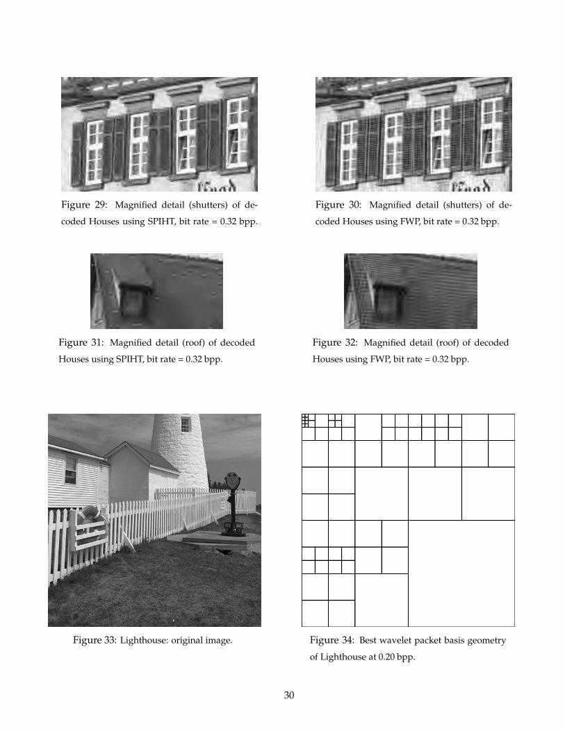
Figure 29: Magnified detail (shutters) of de-

coded Houses using SPIHT, bit rate = 0.32 bpp.

Figure 30: Magnified detail (shutters) of de-

coded Houses using FWP, bit rate = 0.32 bpp.

Figure 31: Magnified detail (roof) of decoded

Houses using SPIHT, bit rate = 0.32 bpp.

Figure 32: Magnified detail (roof) of decoded

Houses using FWP, bit rate = 0.32 bpp.

Figure 33: Lighthouse: original image. Figure 34: Best wavelet packet basis geometry

of Lighthouse at 0.20 bpp.

30

Figure 35: Decoded Lighthouse using SPIHT,

bit rate = 0.20 bpp, PSNR = 26.58 dB.

Figure 36: Decoded Lighthouse using FWP, bit

rate = 0.20 bpp, PSNR = 27.28 dB.

Figure 37: Magnified detail of decoded Light-

house using SPIHT, bit rate = 0.20 bpp.

Figure 38: Magnified detail of decoded Light-

house using FWP, bit rate = 0.20 bpp.

31