NAVAL POSTGRADUATESCHOOL

Monterey, California

THESIS

SPEECH COMPRESSION USING COSINE PACKETDECOMPOSITION

by

Joao Roberto Vasconcellos Martins

Thesis Advisor

Co-Advisor:

March 1996

Monique Fargues

Ralph Hippenstiel

ThesisM3592718

Approved for public release; distribution is unlimited.

DUDLEY KNOX LIBKAKY

NAVAL POSTGRADUATE SCHOOL

MONTEREY CA 93943-5101

REPORT DOCUMENTATION PAGE Form Approved

OMB No. 0704-0188

Public reporting burden for this collection of information is estimated to average 1 hour per response, including the time reviewing instructions, searching existing data sources.gathering and

maintaining the data needed, and completing and reviewing the collection of information. Send comments regarding this burden estimate or any other aspect of this collection of information,including suggestions for reducing this burden to Washington Headquarters Services. Directorate for Information Operations and Reports, 1215 Jefferson Davis Highway. Suite 1204. Arlington!

VA 22202-4302. and to the Office of Management and Budget. Paperwork Reduction Project (0704-0188), Washington, DC 20503.

1. AGENCY USE (Leave Blank) 2. REPORT DATE

March 19963. REPORT TYPE AND DATES COVERED

Master's thesis

4. TITLE AND SUBTITLE

SPEECH COMPRESSION USING COSINE PACKETDECOMPOSITION

6. AUTHOR(S)

Martins, Joao Roberto Vasconcellos

5. FUNDING NUMBERS

7. PERFORMING ORGANIZATION NAME(S) AND ADRESS(ES)

Naval Postgraduate School

Monterey, CA 93943-5000

8. PERFORMING ORGANIZATIONREPORT NUMBER

9. SPONSORING / MONITORING AGENCY NAME(S) AND ADDRESS(ES) 10. SPONSORING / MONITORINGAGENCY REPORT NUMBER

11. SUPPLEMENTARY NOTES

The views expressed in this thesis are those of the author and do not reflect the official policy or position

of the Department of Defense or the United States Government.

12a. DISTRIBUTION / AVAILABILITY STATEMENT

Approved for public release; distribution is unlimited.

12b. DISTRIBUTION CODE

1 3. ABSTRACT (Maximum 200 words)

As digitization of data becomes more prevalent, the demands on existing communications

networks and computer systems to cope with this increase in data become overwhelming. Currently, the

speech compression problem is handled using the CELP( Code Excited Linear Prediction) scheme and its

derivatives. Such techniques are the most frequently used for speech compression at medium-to-low rate

ranges. Recent research conducted into the area of cosine packets has proven this field to be readily

adaptable to speech compression and coding. In this thesis, speech compression schemes are developed

using cosine-packet decomposition, minimum entropy basis selection, and an adaptive thresholding

scheme for selecting coefficients. In addition, voiced-unvoiced segmentation and a denoising scheme were

implemented. Test results showed high compression ratios (1:50) with a good quality of reconstructed

speech.

14. SUBJECT TERMS

Cosine Packets, Wavelet Packets, Speech Compression, Speech Coding15. NUMBER OF PAGES

157

16. PRICE CODE

17. SECURITY CLASSIFICATIONOF REPORT

Unclassified

18. SECURITY CLASSIFICATIONOF THIS PAGE

Unclassified

19. SECURITY CLASSIFICATIONOF ABSTRACT

Unclassified

20. LIMITATION OF ABSTRACT

UL

NSN 7540-01-280-5500 Standard Form 298 (Rev. 2-89)

Prescribed by ANSI Std. 239-18

UNCLASSIFIED

11

Approved for public release; distribution is unlimited.

SPEECH COMPRESSION USING COSINE PACKET DECOMPOSITION

Joao Roberto VasconcelloS/MartinsLieutenant Commander, Brazilian Navy

B.S.E.E., Universidade de Sao Paulo, Brasil, 1986

Submitted in partial fulfillment of the

requirements for the degree of

MASTER OF SCIENCE IN ELECTRICAL ENGINEERING

from the

NAVAL POSTGRADUATE SCHOOLMarch4996///?/ / A /?

DUDLEY KNOX LIBRARY

NAVAL POSTGRADUATE SCHOOLMONTEREY CA 93943-5101

ABSTRACT

As digitization of data becomes more prevalent, the demands on existing

communications networks and computer systems to cope with this increase become

overwhelming. Currently, the speech compression problem is handled using the CELP

(Code Excited Linear Prediction) scheme and its derivatives. Such techniques are the

most frequently used for speech compression at medium-to-low rate ranges. Recent

research conducted into the area of cosine packets has proven this field to be readily

adaptable to speech compression and coding. In this thesis, speech compression schemes

are developed using cosine-packet decomposition, minimum entropy basis selection, and

an adaptive thresholding scheme for selecting coefficients. In addition, voiced-unvoiced

segmentation and a denoising scheme are implemented. Test results show high

compression ratios (1:50) with a good quality of reconstructed speech.

VI

TABLE OF CONTENTS

I. INTRODUCTION 1

II. INTRODUCTION TO SPEECH PROCESSING 3

III. THE LOCAL TRIGONOMETRIC TRANSFORM 7

A. INTRODUCTION 7

B. THE RISING CUTOFF FUNCTION 8

C. FOLDING AND UNFOLDING 10

D. THE CONTINUOUS LOCAL TRIGONOMETRIC TRANSFORM 13

1. Properties 13

2. The Local Transform 16

E. THE DISCRETE COSINE TRANSFORM 18

F. APPLICATION TO SIGNAL ANALYSIS/SYNTHESIS 19

IV. WAVELET AND COSINE PACKET TRANSFORMS 21

A. INTRODUCTION 21

B. THE WAVELET TRANSFORM 21

C. THE WAVELET PACKET TRANSFORM 23

D. THE COSINE PACKET TRANSFORM 27

V. THE BEST BASIS ALGORITHM 29

A. INTRODUCTION 29

B. THE BEST BASIS ALGORITHM METHOD 29

VI. COMPRESSION AND DENOISING SCHEMES 33

A. INTRODUCTION 33

B. MINIMUM TIME WINDOW SIZE 35

C. VOICED -UNVOICED SEGMENTATION 36

D. ADAPTIVE THRESHOLDING 37

E. DENOISING 38

VII. ENCODING SCHEMES 53

A. THE QUANTIZATION SCHEME 53

B. PROPOSED ENCODING SCHEMES 54

1. Cosine packet coefficient locations 54

2. Segment Indexes 55

C. CODING SCHEMES 56

VIII. TESTS AND RESULTS 57

A. INTRODUCTION 57

B. COMPRESSION SCHEMES RESULTS 57

1. Description 57

2. Experimental Results 59

3. Comments 60

C. DENOISING-COMPRESSION RESULTS 62

1. Description 62

2. Results 62

vn

3. Comments 65

D.ENCODING SCHEMES RESULTS 67

1. Description 67

2. Results 68

E.COMPARISON WITH WAVELET PACKET TRANSFORM 70

IX. CONCLUSION 91

APPENDIX 95

LIST OF REFERENCES 139

INITIAL DISTRIBUTION LIST 141

Vlll

LIST OF FIGURES

Figure 2.1.

Figure 3.1.

Figure 3.2.

Figure 3.3.

Figure 3.4.

Figure 3.5.

Figure 3.6.

Figure 3.7.

Figure 3.8.

Figure 4.1.

Figure 4.2.

Figure 4.3.

Figure 4.4.

Figure 4.5.

Figure 4.6.

Figure 4.7.

Figure 4.8.

Figure 4.9.

Figure 5.1.

Figure 5.2.

Figure 5.3.

Figure 5.4.

Figure 6.1.

Figure 6.2.

Figure 6.3.

Figure 6.4.

Figure 6.5.

Figure 6.6.

Figure 6.7.

Figure 6.8.

Figure 6.9.

Figure 6.10.

Figure 6.11

Figure 6.12.

Figure 8.1.

Figure 8.2.

Figure 8.3.

Figure 8.4.

Figure 8.5.

Figure 8.6.

Sound "ISSOS", male non-native speaker 6

Arbitrary partition of time into adjacent intervals 8

Overlapping windows of arbitrary size 8

The rising cutoff function 9

Unfolding operator in a block cosine 11

Block cosine and block sine after periodic folding 12

Two child bells overlapped and one inverted parent bell 13

Three different bells 14

Fourier transforms of the bells of Figure 3.6 15

WT Implementation: A bank ofQMF pairs 22

Wavelet transform: decomposing 2J samples into a max. ofj levels 22

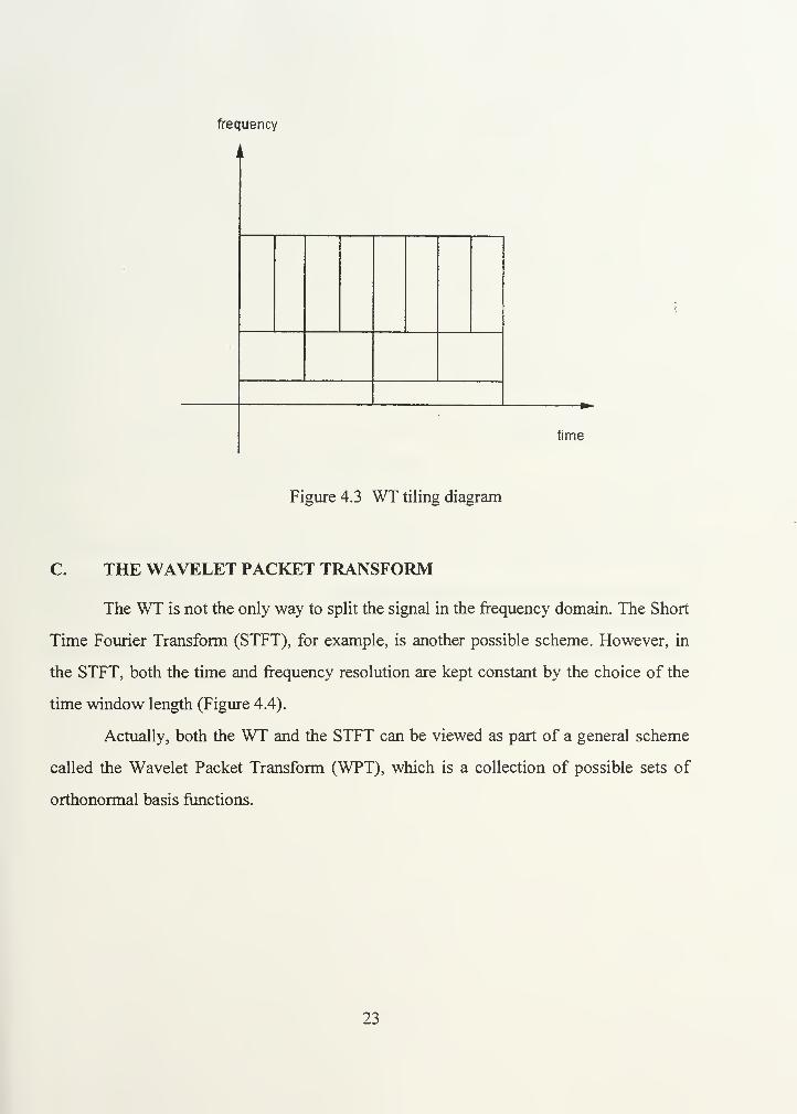
WT tiling diagram 23

Tiling diagram for the STFT 24

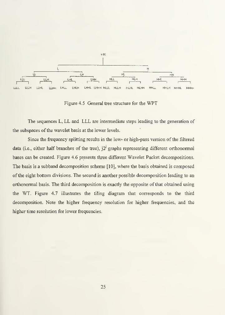
General tree structure for the WPT 25

Three different WP decompositions leading to three different bases 26

Tiling diagram for the decomposition of figure 4.6c 26

Cosine packet transform: The tree configuration 27

Tiling diagram corresponding to figure 4.8 28

Cosine packet tree with computed entropies for every interval 30

New (and former) computed entropy for each node 31

Selection ofminimum entropy basis 31

Best basis tiling scheme resulting from the decomposition in Fig. 5.3 32

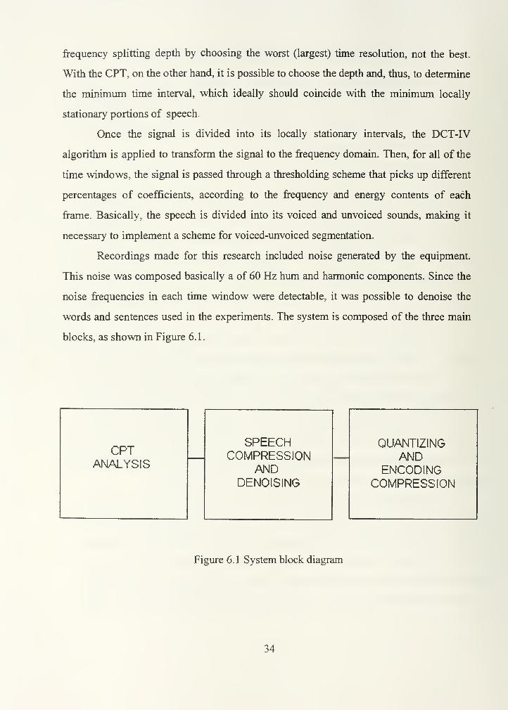
System block diagram 34

"This Place Blows": Short-time energy and zero-crossings 41

"This Place Blows": Time/ Frequency behavior/ Energy / Spectrogram 42

"This Place Blows": Time/ Voiced-unvoiced segmentation/ Spectrogram 43

"Be Nice to your sister": ST Energy/ Zero-crossings/ Time plots 44

"Be Nice to your sister": Time/ Frequency/ Energy/ Spectrogram 45

"Be Nice to Your Sister": Time/ Voiced-unvoiced/ Spectrogram 46

"Nice": fixed thresholding, 1% coefficients kept for compression 47

"Nice": adaptive thresholding, 0.98% coefficients kept 48

"Hey": /h/ lost after denoising scheme when it is identified as noise only 49

"Hey": /h/ recovered after denoising scheme when identified as speech 50

"Cats": /s/ lost after denoising scheme when identified as noise only 51

" Be": Time plots/ spectrograms before and after den./comp 72

" Hey",male: Time plots/ spectrograms before and after den./comp 73

" Hey",female: Time plots/ spectrograms before and after den./comp 74

" Pay",female: Time plots/ spectrograms before and after den./comp 75

" Pay",male: Time plots/ spectrograms before and after den./comp 76

" Hello...": Time plots/ spectrograms before and after den./comp 77

IX

Figure 8.7.

Figure 8.8.

Figure 8.9.

Figure 8.10.

Figure 8.11.

Figure 8.12.

Figure 8.13.

Figure 8.14.

Figure 8.15.

Figure 8.16.

Figure 8.17.

Figure 8.18.

1

Bye...": Time plots/ spectrograms before and after den./comp 781

Project": Time plots/ spectrograms before, after den./comp./decoding 79: Be nice...": Denoising/ compression / decoding /16-level quantizer 80; Be nice...": Denoising/ compression / decoding /32-level quantizer 81; Be nice...": Denoising/ compression / decoding /64-level quantizer 82

Bye...": Denoising/ compression / decoding / 16-level quantizer 83:

Bye...": Denoising/ compression / decoding / 32-level quantizer 84:

Hey": Denoising/ compression / decoding / 16-level quantizer 85;

Hey": Denoising/ compression / decoding / 32-level quantizer 86' Hey": Denoising/ compression / decoding / 64-level quantizer 87' Be Nice...": Compression with CPT, ndencomp implementation 88; Be Nice...": Compression with WPT 89

x

LIST OF TABLES

Table 6.1. Frequency range and display 36

Table 8.1. Mean opinion score table 59

Table 8.2. Compression only results 61

Table 8.3. Compression results utilizing codes ndencomp.m and encp6.m 63

Table 8.4. Denoising/compression results 64

Table 8.5. Speech quality mean grades 64

XI

Xll

ACKNOWLEDGMENTS

First, to my wife Monica, all my gratitude. Her sacrifice, patience, care, support

and words of encouragement made the crossing of this river much easier and less

turbulent. To my daughter, Bruna, she is a great gift that I've received. I thank her for

reminding me of how beautiful and joyfull life can be. I also thank my parents, Joaquim

and Norma, for all their support throughout my life.

It was a great pleasure having the opportunity to work with and learn from such

high quality professors. I truly enjoyed Dr. Roberto Cristi's courses on Signal Processing

and Image Compression Techniques. It was a pleasure to be introduced to Speech

Processing by Dr. Charles Therrien. To Dr. Ralph Hippenstiel, my co-advisor, thanks for

all his support and encouragement. I enjoyed every one of his courses. Very special

thanks to my thesis advisor, Dr. Monique Fargues. Her help, guidance, dedication and

trust gave me the motivation to complete this work. Thanks to Mercedes of the

curriculum office for keeping me on the right track.

To my sponsors and friends, Ronald and Susan, Mauricio and Cristina, Doug and

Denise, thank you for your support and friendship. We were destined to meet and become

friends. To Altay, Mucahit, Manos, Nabil and Soonho, good luck wherever life leads

them. They have proved that friendship has no language, no nationality.

Finally, I thank God for giving me this unique opportunity to learn and live with

my family in beautiful and peaceful Monterey, California. It is a gift I will always

remember.

xni

I. INTRODUCTION

Speech compression allows smaller bandwidth, higher data rates or a combination

of these atributes. It can also be used to store speech like data in a compact form.

This thesis develops speech compression schemes based on the Local

Trigonometric Transform [2], which use an adaptive thresholding scheme proposed in

this work. These schemes perform a time partition of the original speech data first,

according to a maximum depth selected by the user. An experimentally derived, optimum

depth is proposed, based on the results of tests with several words and phonemes (defined

in Chapter II). Following the time partitioning, a basis obtained via the mimmum entropy

best basis algorithm is selected. In order to perform compression, coefficients are selected

according to an adaptive thresholding scheme, which varies the compression percentage

depending on the energy and frequency content of each interval. The intervals are

classified by a voiced-unvoiced segmentation algorithm. Depending on their

classification, selection of coefficients is made in such a way that more coefficients are

preserved for the voiced than for the unvoiced intervals. Then, these coefficients are

encoded using uniform quantizers and Huffman coding to achieve average compression

ratios of 1:50. In addition, two denoising schemes are proposed to minimize effects of

equipment noise below 120 Hz, thereby improving the sound quality.

In a typical scenario, users of the proposed schemes will be able to adjust speech

quality and transmission bandwidth, based on the current channel bandwidth available.

They will be provided with the parameters that maximize the compression ratio, and

minimize the required bandwith at an acceptable speech quality. Using lower bit rate

coding reduces the transmission bandwith of the signal and may prove to be quite useful

in partial band jamming environments where the available channel bandwidth may be

limited. It is understood that the schemes proposed may be useful for military

applications where the understanding of the message is more important than the overall

quality of the sound. This thesis concentrates on finding the best possible compression

ratio, while still keeping an acceptable sound quality. In this work, sound quality is

defined in terms of a mean square error as well as in terms of a proposed quality measure.

Extentions of the proposed techniques lead to data storage improvements and they can

also easily be adopted to cryptographic applications. The thesis is organized in the

following manner. Chapter II presents an introduction to speech processing, where the

concepts of phonemes and coarticulation effects are introduced and illustrated. Chapter

III introduces the Local Trigonometric Transform and presents the Local Cosine

Transform adopted in our work. The Local Cosine Transform can be viewed as a basic

building block for the more complex Cosine Packet Transform, which has been used

recently in speech applications [2]. The Cosine Packet Transform can also be viewed as a

dual operation of the Wavelet Packet Transform [2]. Both packet schemes are presented,

discussed and compared in Chapter IV. The Wavelet and Cosine Packet Transforms

involve the selection of a particular basis "best" matched to the signal under study for

compression applications. This choice of basis is carried out via the Best Basis algorithm,

which is presented in Chapter V. Chapter VI presents the denoising and compression

schemes investigated in this work. Denoising allows for enhancement of the audio quality

of the speech signals when noise is present. Chapter VII describes the encoding schemes

used to compress the speech information. Chapter VIII first discusses the experiments

and parameters used to test our denoising and compression schemes. Next, it presents the

results obtained using various phonemes, words and sentences. The data base consists of

a limited collection of American-English words, some Portuguese words and some

typical voiced and unvoiced sound segments. Some of the more elaborate data sets

consist of complete sentences and dialogues. Finally, we compare compression results

obtained with our Cosine Packet scheme and those obtained with the Wavelet Packet

scheme using a "Daubechies" basis function [17]. Results show that the Cosine Packet

Transform outperforms the Wavelet Packet Transform on the speech segments considered

in this study. Finally, Chapter IX contains the conclusions and final considerations. All

computer algorithms are listed in the Appendix.

II. INTRODUCTION TO SPEECH PROCESSING

One of the principal differentiating features of any speech sound is excitation [1].

Two elemental excitation types are present in speech data: (1) voiced and (2) unvoiced.

Voiced sounds have high energy and low frequency, while unvoiced sounds have low

energy and high frequency. Another important characteristic of speech signals is that they

are locally stationary.

The basic theoretical unit for describing how speech conveys linguistic meaning is

called a phoneme. Each language has its own set of phonemes. For example, American

English has about 42 phonemes, while Brazilian Portuguese has about 5 1 phonemes (Rio

de Janeiro region). They are made of vowels, semivowels, diphthongs, and consonants. In

general, the duration of each phoneme may vary from 1 5 to 400 milliseconds, depending

on the sound produced and the way it is pronounced. For example, vowels can vary

largely in duration, typically from 40 to 400 milliseconds.

The transition from one phoneme to another is not made abruptly or

independently of adjacent phonemes. Actually, adjacent phonemes have a strong

influence on the manner in which the transition takes place. The term used to refer to the

change in phoneme articulation and acoustics that is caused by the influence of another

phoneme is coarticulation.

Since this research investigates speech compression, there are two main

requirements. First, we need to be able to split a speech signal into its smallest locally

stationary "cells" constituted by phonemes, and represent them in a minimal way with

good fidelity. Second, we need to preserve coarticulation effects as much as possible (i.e.,

we need to preserve the smooth transition from one phoneme to the next) .

Figure 2.1 illustrates the coarticulation process for the sound /issos/. The top plot

represents time-domain speech. The middle plot represents the voiced and unvoiced

portions of this sound obtained using the zero-crossing rate and the short-time energy

contained in the sound [1]. The unvoiced portions are -ss- and -s-, corresponding to the

phoneme Isl. The high frequency and low energy of unvoiced segments are illustrated by

the low short-time energy and high zero-crossing rates. The voiced portions of the sound

are the phonemes I'll and lol. The low frequency and high energy of voiced phonemes are

illustrated by the high short-time energy and low zero-crossing rate. The bottom plot

shows the spectrogram obtained using a Harming time window of length 256 samples

with an overlap of 128. Note the coarticulation effects present, which allow for smooth

transitions between phonemes. For example, the transition from lil to Isl occurs through a

"link," which takes place in a high frequency portion of the spectrum, and which is an

example of anticipatory coarticulation (or right-to-left coarticulation). This means that the

articulator has moved from the present phoneme (lil) toward a position (higher frequency)

that is more appropriate for the following phoneme (Isl).

"ISSOS"

1000 2000 3000 4000 5000 6000

Time samples

Short-time Energy and Zero Crossings

7000

0.1 0.2 0.3 0.4 0.5 0.6

Time (seconds)

0.7 0.8 0.9

8000

Observing The Coarticulation Process for "ISSOS"

3000 4000 5000

Time samples

6000 7000 8000

Figure 2.1 Sound "ISSOS," male non-native speaker; top plot: Time domain

representation; middle plot: Short time energy and zero-crossing representation;

bottom plot: Spectrogram of "ISSOS" using a Hanning time window of length 256

samples with overlap 128, fs = 8 KHz.

III. THE LOCAL TRIGONOMETRIC TRANSFORM

This chapter discusses the main concepts related to the Local Trigonometric

Transform theory and its implementation. Much of the mathematical rigor is omitted, and

emphasis is placed on the basic theory and its application to speech processing. This

chapter is divided into six sections. The first provides an introduction, and the second

presents some basic definitions about the rising/cutoff function. The third section defines

the folding and unfolding operations that are used for the transform [2]. The fourth

describes the Continuous Transform and its main mathematical properties. The fifth

defines the Discrete Transform. Finally, the last section applies these concepts and

describes how the transform may be performed by using orthonormal bases to allow for

signal analysis and synthesis.

A. INTRODUCTION

In order to analyze small portions of the speech signal, it must be partitioned in

time. The local transform defined in this chapter applies a "local cosine," which is a basis

function that allows the signal to be cut into time slices. As first defined by Malvar in

1987 [3], the "local cosines" provided a regularly spaced partition in time. Later, Coifman

and Meyer [4] and Meyer [5] tackled the problem of modifying regular constructions to

obtain windows with variable lengths that could be defined arbitrarily. They began by

partitioning time into adjacent intervals [otj otj+1 ], as illustrated in Figure 3.1. Figure 3.2

shows in more detail how the windows may be combined while still preserving the

smoothness and integrity of the signal. The windows used are essentially the intervals [cij

Oj+1 ]. The disjoint intervals [ctj - Sj , otj + Sj ] allow the windows to overlap. In summary,

the local cosines (called "Malvar wavelets") are constructed with a rising duration (28j), a

stationary period (At), and a decay (which lasts 28j +L)- The ability to arbitrarily and

independently choose the duration of the rising and decaying, as well as the stationary

section, is exactly what makes the Malvar wavelets different from other well-known

wavelets (e.g., Gabor or Daubechies) [5]. Of course, it is important to use this ability

efficiently. This choice will be discussed in the following chapters, where we focus on the

best basis for decomposition of the signal.

Jo h h

Qri a2 a3

h h

a4

Figure 3 . 1 Arbitrary Partition of Time into Adjacent Intervals

ujj-iit) ujj(t) Wj+i(t)

' 2ei ' At

Figure 3.2 Overlapping windows of arbitrary size

B. THE RISING / CUTOFF FUNCTION

The well-known Discrete Cosine Transform (DCT) has, as its basis function, a

"block cosine" (i.e., a rectangular window that multiplies the cosine function). The

functions obtained by the block cosine result in a discontinuity or an abrupt variation in

the signal. As a result, we have discontinuities at the block boundaries of the reconstructed

signal. The effects produced include the so-called "blocking effect" in image coding, and

the "clicking sounds" in speech coding [6]. These problems can be avoided by defining a

window based on a function that allows for a smooth transition from zero to the amplitude

of the cosine (on the left edge), as well as from that amplitude to zero (on the right edge).

The function r is defined as r = r{t) in the class C d(R), for some 0<d<oo,

satisfying the following conditions:

0, if t< -1,•(*)

I +I

r(-t)|

2 = 1 for all t € R; r(t) =(3.1)

1, if t> 1.

It is called a rising cutoff function because r{t) monotonically increases from zero to one

over the domain of t from - oo to + oo. That function is presented in Figure 3.3.

1

0.9

0.8

0.7

0.6

0.5

0.4

0.3

0.2

0.1

n

1

•

i

1/ i

7

i

i "i /i /

1i

' /i /

! !/i

A!

i

1 /// 1 ! !

I

I

I /1

i

|

i yi Jr^ I I I I

10 20 30 40time

50 60 70

Figure 3.3 The rising cutoff function

C. FOLDING AND UNFOLDING

The folding operator Uand its adjoint unfolding operator U* are defined as follows:

' r(t)f(t) + r(-t)f(-t), if t >Uf(t) =

\ (3.2)

I r(-t)f(t)-r(t)f(-t), if t<0

r(t)f(t)-r(-t)f(-t), if t>0 nTll7V(i) = <|

(jJ)

r(-t)f(t)+r(t)f{-t), if *<0.

Observe that £//(/) = /(/), and C/*/(0 =/(0 - if *> 1 or if t < -I. Also, U*U fit) =

UU*f(t)= (|r(r)P+ \r(-t)\2

) f(t)=f(t), forall^ 0, so that Uand t/* are

isomorphisms ofI (7?). This means that one operator is the inverse of the other.

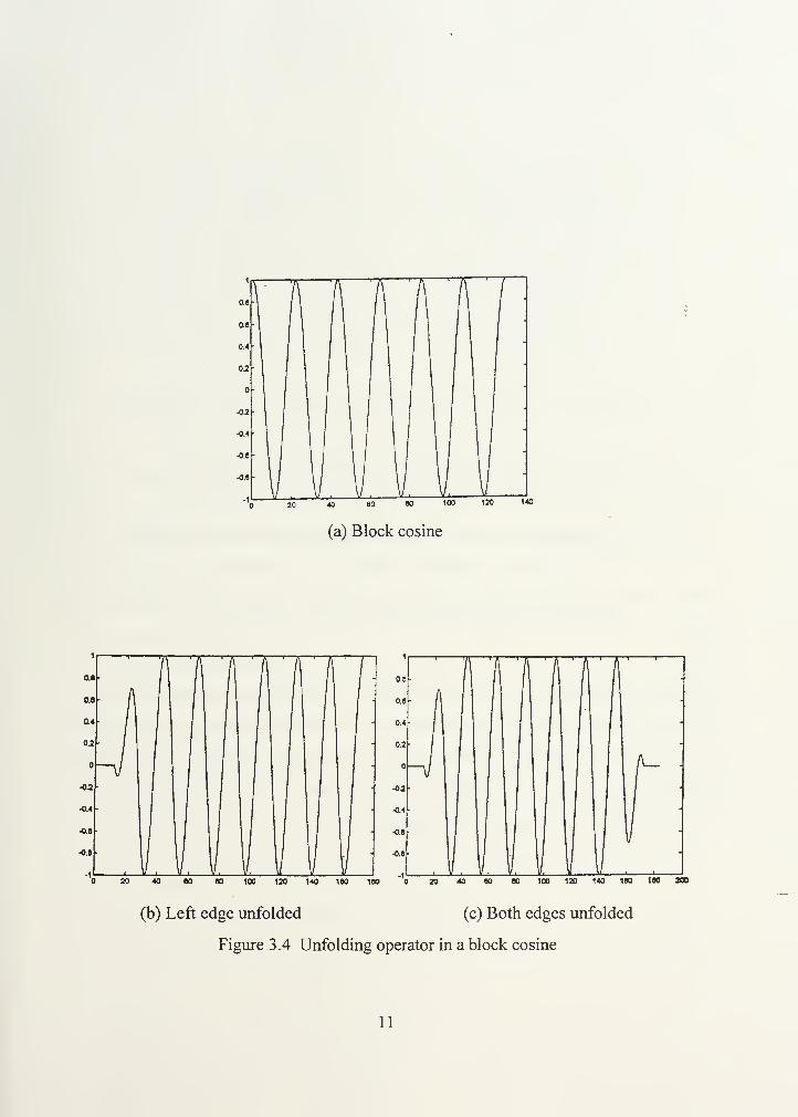
Figure 3.4 illustrates the unfolding operation on a block cosine. Figure 3.4a shows

a block cosine. Figures 3.4b and 3.4c illustrate the cosine unfolded at its left edge, and

unfolded at both edges, respectively.

Figure 3.5 presents a block cosine and a block sine after periodic folding. The

purpose of folding is to prepare the function intervals, so that the adjacent windows can be

overlapped further without changing the function in the overlapping interval.

10

100 120 140

(a) Block cosine

30 40 BO 80 100 120 140 180 160 300

(b) Left edge unfolded (c) Both edges unfolded

Figure 3.4 Unfolding operator in a block cosine

11

100 120

(a) (b)

Figure 3.5 (a) Block cosine and (b) Block sine, both after periodic folding

To extend the concept of folding and unfolding in an interval, the operators now

can be shifted and dilated so that their action takes place on an arbitrary interval (a - s, a

+ e). Now, after partitioning the time by periodically folding the left and right edges of

each interval, all the adjacent component windows can be unfolded and overlapped. The

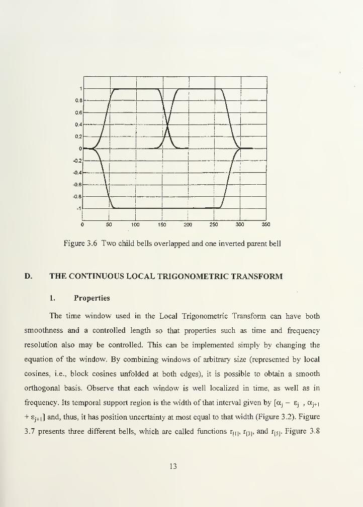
window formed by the rising cutoff function is called a bell. Figure 3.6 displays two small

bells (called child bells) overlapped and one inverted large bell (called the parent bell)

below, showing that it is possible to preserve both the smoothness between intervals and

the signal integrity (with no loss of information), if each interval is unfolded and then

overlapped. This explains how parent windows may be split into two child windows (in

the decomposition phase), and how two child windows may be combined to form one

parent window (in the reconstruction phase). This property is particularly important when

the concept of the "cosine packets" is introduced.

12

0.8

0.6

0.4

0.2

-0.2

-0.4

-0.6-

-0.8

50 100 150 200 250 300 350

Figure 3.6 Two child bells overlapped and one inverted parent bell

D. THE CONTINUOUS LOCAL TRIGONOMETRIC TRANSFORM

1. Properties

The time window used in the Local Trigonometric Transform can have both

smoothness and a controlled length so that properties such as time and frequency

resolution also may be controlled. This can be implemented simply by changing the

equation of the window. By combining windows of arbitrary size (represented by local

cosines, i.e., block cosines unfolded at both edges), it is possible to obtain a smooth

orthogonal basis. Observe that each window is well localized in time, as well as in

frequency. Its temporal support region is the width of that interval given by [oCj - Sj , Oj+1

+ 8j+1 ] and, thus, it has position uncertainty at most equal to that width (Figure 3.2). Figure

3.7 presents three different bells, which are called functions r^j, r[3 j,

and r[5]

. Figure 3.8

13

presents the positive half of the real part of the Fourier Transform of the functions given in

Figure 3.7.

as

08/ \

0.7

/ \OS

/ \08

/ \04

/ \

03/ \

02 " / \

0.1

J 1 I ! 1 \ t

80 100 120 140

(a)

100 120 140 140 180

(b) (c)

Figure 3.7 Three different bells; (a) r^; (b) r[3] ;

(c) r[51

Note that the sidelobes increase as the roll-off of the time window

increases.

14

20 40 SO 80 100 120 140

(a)rID

90 -

1 1 1 1

•0 •

40

20

1 I

-30

-il k--vy r

-40

-20 40 80 80 100 120 140 180 180

(b)r.[3]

(c)r[5]

Figure 3.8 Fourier transforms of the bells of Figure 3.7

15

2. The Local Transform

The Continuous Local Trigonometric Transform is based on a set of orthonormal

basis functions that allow for a variable-length time window while still maintaining a

small time-frequency bandwidth product. The Transform can be either a local cosine or a

local sine. Since the local cosine has been chosen, the definition of the so-called "block

cosine" at half-integer frequency is given as follows:

C„ (t) = cos [n(n+ 1/2) t] , (3.4)

where n is an integer, and / is restricted to the interval [0,1].

As can be observed from the right side of Figure 3.4c, unfolding the block cosine

at the edges gives it the necessary smooth characteristics that contribute to a good

frequency resolution for that transform. Basically, smoothness is obtained by a smooth

cutoff by sine iteration [2], defined by:

' 0, if t < 1

,

sin [j(l + 0] ,if -1 < t < 1, andr«»(0 ={

I 1, if t > 1, , „

7"(0j = r 5tn (0 and 7-(l+1 |= 7-j,] (sin - t

(3.5)

(3-6)

Since r^j is smooth on (-1,1) with one vanishing first derivative at the boundary

points, the envelope (referred to as the bell in [5]) has a continuous derivative on R . Based

on the recursion in Equation (3.6), r^ can be used with i > 1 to obtain additional

derivatives [5]. Actually, it can be shown that r^/) has 21_

vanishing derivatives, rm is

used, since it allows good resolution and has very small side lobes.

Thus, the local cosine is defined as :

V'njt — a, <y

(Y7 + 1 a,

7 + 1

7+1- t

7+1COS

(n+m-otj)<*j+i ~

<*J

(3.7)

16

where otj and ctj +1 are the interval edges, Sj and Cj+1 are the action radii of the operators for

both edges, and r-}

, rj+1 is the rising function rtl ],

applied at both edges of the interval. Note

that the local cosine as defined by Equation (3.7) is the result of the unfolding operation at

both edges of the "block cosine," i.e.,

¥nj(0 = uVjiCtj, Gj) U (r]+x a i+lei+l )

A u (t)Cnj(t),

where:

•lu(0 Cn j(?) represents the block cosine function for an interval beginning at

edgej;

•U*(.) is the unfolding operator applied at the left (j) and right edge (j+1) of

the interval.

Thus, the Continuous Local Trigonometric Transform is the inner product (f,vj/ n :),

where \j/ n j is the local cosine defined above.

Instead of computing in that manner, one may fold the function first, and then

obtain the inner product with the regular "block cosine," as in the expression below:

av|/nJ > = <C/jC7j+1 /l IJ CnJ >. (3.8)

In practice, this simple observation has great importance, since it means that/can

be preprocessed by folding, and the local cosine transform can be computed with an

ordinary cosine transform [2].

It is also important to observe that, by defining the transformation as an inner

product, what is measured is the amount of "similarity" between the signal /(r) and the

basis function Cn j. This is one of the key attributes that make the local cosine transform

convenient for the transformation of speech signals and, therefore, good for compression

and coding. The fact that speech can be considered a locally stationary signal with a

17

reasonable correlation to sines and cosines may explain some of the good results when

using a Local Trigonometric Transform.

E. THE DISCRETE COSINE TRANSFORM

By replacing just the variables with integers, and by using the discrete cosine

transform, it is possible to obtain discrete versions of the local cosine. So Equation (3.9) is

exactly the same formula as Equation (3.7), but with the variables replaced by integer

values. In Equation (3.9) it is assumed that:

• Oj< Oj+1 , where otj andaj+1 are integers;

• the signal is sampled at integer points t, Oj < t < Oj+1 , which gives (ccj+1- ctj)

samples;

• >j and /j+1 are the rising functions rfl ]

, applied at both edges of the interval;

• £j > and Sj+i > 0, with Sj + £j+1 < number of samples to insure that the action

regions are disjoint.

Equation (3.9) also makes a distinction between the left and right endpoints,

because sampling is done at the left endpoint of each interval. If sampling is done in the

middle of the intervals (which can be done by taking the function in Equation (3.7) and

replacing every instance of t with t+1/2), it will be more symmetric, and the basis

functions will be cosines sampled between grid points. The result is the following discrete

local cosine basis function:

**«—»-*PVM2*^)<Xj+i - a

;

cos (3.9)

18

F. APPLICATION TO SIGNAL ANALYSIS/SYNTHESIS

Given an arbitrary partitioning of a signal in time, it is possible to construct several

smooth orthogonal bases, using the local cosine transform as the basis function. The

scheme that leads to the best partition and the best basis for this application will be

introduced in the next chapter. This section explains how the DCT-IV can be used for an

analysis in the frequency domain and for further synthesis in the time domain.

As mentioned in sections "C" and "D", the signal is first folded at the left and

right ends of each interval. Then, an ordinary DCT-IV transform is used to compute the

Local Cosine Transform for each of the windows obtained. Now, it becomes possible to

analyze each time window using the frequency spectrum (from DC to fs/2, where f

sis the

sampling frequency). To reconstruct the signal, the DCT-IV is applied to obtain the

inverse. As in the decomposition phase, the transform is computed first with the regular

"block cosine," and then the intervals are unfolded, instead of using the local cosine. By

periodically unfolding the left edges of the current interval and the right edge of the

following one, the smoothness and integrity of the function are preserved, allowing the

time domain function to be reconstructed.

19

20

IV. WAVELET AND COSINE PACKET TRANSFORMS

This chapter presents the Wavelet Transform and two general time-frequency

analysis schemes: the Wavelet Packet Transform and the Cosine Packet Transform .

A. INTRODUCTION

The goal of this thesis is to obtain the scheme best suited for the decomposition

and reconstruction of speech signals, in particular, one that can decompose a speech

signal into an orthonormal basis function. First, the Wavelet Transform (WT) and its

main properties and characteristics are discussed. Next, the general concept of the

Wavelet Packet Transform (WPT) is introduced. Finally, the Cosine Packet Transform

(CPT) is presented. This last scheme initially performs a time split, as opposed to

transforms that first split the signal in the frequency domain.

B. THE WAVELET TRANSFORM

In the Wavelet Transform (WT) algorithm, the sampled data set is passed through

the low-pass and high-pass filters with complementary bandwidths, known as quadrature

mirror filter (QMF) pairs [7]. The outputs of both filters are decimated by a factor of two.

So, at each scale, we have a set of high-pass filtered data and a set of low-pass filtered

data. Each of these sets has half as many elements as the original data set, as a

consequence of the decimation. The low-pass filtered data can be used as the data input

for another pair of filters identical to the first pair, generating another set of low- and

high-pass coefficients at the next lower level of scale [8].

This process can continue until the set of original coefficients has been reduced to

the minimal scale level, which is two coefficients. Figure 4.1 presents the pyramid

algorithm of the WT. Figure 4.2 shows how a unit interval of length 2J samples can be

decomposed to obtain a maximum of j levels of transform data. Figure 4.3 presents the

tiling diagram that corresponds to the WT decomposition. This shows that the WT works

well if the signal is composed of strong components of short duration, i.e., bursts. This

21

means that the WT is a good detector of transients. It also works well if the signal is

composed of low-frequency components of long duration [9].

As stated earlier, speech is composed of portions of either high frequency or low

frequency, both with a typical minimum duration of about 15 milliseconds. These

characteristics indicate that the WT may not be the best scheme for speech signal

analysis.

21 2:1 21 21 21

LP LP LP LP LP

21

•— HP

21

HP

Level

LLLLH

LLLH

Level 1

21

HP

21

HP

LLH

Level 2

LH

Level 3

21

HPLevel 4

Figure 4. 1 WT implementation: A bank ofQMF pairs

y ( 2J samples )

I

LH

LLH

LLLHLLLLL LLLLH

Figure 4.2 Wavelet transform: decomposing 2J samples into a maximum of j levels

22

frequency

11

time

C.

Figure 4.3 WT tiling diagram

THE WAVELET PACKET TRANSFORM

The WT is not the only way to split the signal in the frequency domain. The Short

Time Fourier Transform (STFT), for example, is another possible scheme. However, in

the STFT, both the time and frequency resolution are kept constant by the choice of the

time window length (Figure 4.4).

Actually, both the WT and the STFT can be viewed as part of a general scheme

called the Wavelet Packet Transform (WPT), which is a collection of possible sets of

orthonormal basis functions.

23

frequency

time

Figure 4.4 Tiling diagram for the STFT

Figure 4.5 depicts the general tree structure for the WPT. Note that the heavy lines

indicate the graph that forms the WPT basis. The symbol L or H has been assigned to

each half frequency division, depending on whether it is a high- or low-frequency band.

Following the tree structure, we have assigned those symbols sequentially, following the

same rule. Note that the WT basis consists of the subspaces H, LH, LLH, LLLH and

LLLL.

24

y(K)

U- LH HL HHI

J1

I"J

11 L_

LLL LLH LHL LHH HLL HLH HHL HHH-|

|

'

1 I 1 I I I I | 1 I II 1

LLLL LLLH LLHL LJLHH LHLL LHLH LHHL LHHH HLLL HLLH HLHL HLHH HHLL HHLH HHHL HHHH

Figure 4.5 General tree structure for the WPT

The sequences L, LL and LLL are intermediate steps leading to the generation of

the subspaces of the wavelet basis at the lower levels.

Since the frequency splitting results in the low- or high-pass version of the filtered

data (i.e., either half branches of the tree), j2J graphs representing different orthonormal

bases can be created. Figure 4.6 presents three different Wavelet Packet decompositions.

The basis is a subband decomposition scheme [10], where the basis obtained is composed

of the eight bottom divisions. The second is another possible decomposition leading to an

orthonormal basis. The third decomposition is exactly the opposite of that obtained using

the WT. Figure 4.7 illustrates the tiling diagram that corresponds to the third

decomposition. Note the higher frequency resolution for higher frequencies, and the

higher time resolution for lower frequencies.

25

(a)

¥00

iL itL HL HH

LLH •LHl LHH HLL HLH HHL HHH

(b) ¥00

LL •LH HL HH

HLL HLH_l_

HHL HHH

II

HLLL HLLH HLHL HLHH

V(k)

(c)

Hi

HL HH

HHL HHH

1 1

HHHL HHHH

Figure 4.6 Three different wavelet packet decompositions leading to three different bases

frequency A

time

Figure 4.7 Tiling diagram for the decomposition of figure 4.6c

26

D. THE COSINE PACKET TRANSFORM

The Cosine Packet Transform (CPT) is a scheme that allows for a time-splitting

decomposition prior to the frequency transformation. If one imagines the original signal

in the time domain being split successively into two halves at each iteration, a tree

configuration will result (Figure 4.8). If the transform imposes no restriction on the

support intervals of the window envelopes, the tree does not need to be homogeneous.

This means that the windows do not need to be combined in the same way (either in pairs

or in any other specific manner). Also, the subspaces do not need to be of equal size. So,

in analogy to the wavelet packets case, one is now faced with a large number of possible

orthonormal basis configurations, each one of them being considered as a cosine packet.

It is important to observe that in the cosine packets case, the windows do not need to be

of a dyadic size, they may be of an arbitrary size. However, in this thesis, only dyadic

sized windows are considered.

Levels

Figure 4.8 Cosine packet transform: The tree configuration

We also note that, as one goes down the tree, time resolution is improved by a

factor of two at each layer, while frequency resolution is decreased by a factor of two at

time

27

each iteration. Figure 4.9 presents the tiling diagram that corresponds to the tree

configuration shown in Figure 4.8. The CPT works in such a way that, after time splitting

to a certain depth, a basis is selected by some criterion. Then, for each time window, the

DCT-IV transform is applied.

frequency

A ....

time

Figure 4.9 Tiling diagram corresponding to Figure 4.8

28

V. THE BEST BASIS ALGORITHM

A. INTRODUCTION

When a choice of bases exists for the representation of a signal, it is possible to

determine the best one using some predetermined criterion. The criterion will always

depend on the type of signal and the user's objective. In this case, the signal is speech

and the objective is to minimize the number of symbols used to represent the information

contained in a given interval (i.e., it is desirable to minimize the entropy of that interval).

The "best basis" criterion allows for the minimization of some information costs options,

including the entropy minimization method [6,1 1].

We recall that the entropy of a vector u = { u(k) } is defined by :

#(«) = !/>(*) log(l //**)), (5.1)

where p(k) =|u(k)

|/ \\u\\ is a normalized energy of the k element of the sequence, and

p log 1/p is set to 0, ifp = 0. H(u) is the entropy of the probability distribution function

(or pdf) given by p. Note that H(u) is not a an information cost functional, i.e., it is not a

direct function of the sequence (u(k)}. But the functional

/(«) = LK*)l2log(l/| M(*)|

2

)

is a direct function. If l(u) is minimized, then H(u) is also minimized in the expression:

i/(u) = ||u|r2/(u) + log||u||

2. (5.2)

B. THE BEST BASIS ALGORITHM METHOD

Initially, the algorithm computes the entropy obtained in all intervals or "nodes"

of the tree. Figure 5.1 presents an example of the cosine packet tree with corresponding

computed entropies. The Best Basis Algorithm searches the tree in a bottom-up direction

29

and, whenever a parent node has a lower cost than that of its children, the Best Basis

algorithm flags the parent. If the sum of the children's costs is lower than that of the

parent node, this lower cost is assigned to the parent. Similarly, children are flagged when

they have a lower information cost than their parents. This step avoids the need to

examine any node more than twice: once as a child and once as a parent. Figure 5.2

presents the new and the former (in parenthesis) information costs for each node shown in

Figure 5.1. Then, after all nodes present in the tree have been examined, the Best Basis

Algorithm selects the topmost flagged nodes, which constitute a basis. Finally, as the

topmost flagged node is encountered, the remaining nodes in the corresponding subtree

are discarded. Figure 5.3 displays the best basis nodes for this example as shaded blocks.

Further details may be found in [4]. Figure 5.4 shows a Best Basis tiling scheme resulting

from the decomposition shown in Figure 5.3. It is obvious that each resulting cell

occupies one portion of the time, and the whole frequency spectrum is covered by each of

those cells.

/ ^"--^XL2 ^^-"" \^

f ^<X26 X 27 y^\ \s* v

*"v~

X3 >X

X X- X "X X ( "X X/ \

->c7\y X/ \ I \/^yx 'X-

v

>\ ' A 8 \

Figure 5.1 Cosine packet tree with computed entropies for every interval (node)

30

^xrx^xFigure 5.2 New (and former) computed entropy for each node

35 (52)

3(10)

r^l^

10(26)

7(12)

25 (27)

1 1 (1 3)

A JXy\

v?x/*y/s

X ~7 \

Figure 5.3 Selection of minimum entropy basis

31

frequency

1 1

time

Figure 5.4 Best basis tiling scheme resulting from the decomposition in Figure 5.3

32

VI. COMPRESSION AND DENOISING SCHEMES

This chapter describes the compression and denoising schemes used in this

research. It is divided into five sections. First, the motivating concepts are introduced. In

the remaining sections: minimum time window, voiced-unvoiced segmentation, adaptive

thresholding and denoising are presented.

A. INTRODUCTION

Initial research for this thesis included reviewing existing lossy compression

techniques, which are divided into two main classes: Lossy Predictive Coding and

Transform Coding [12]. The attention of this thesis is directed to Transform Coding. The

Transform Coding technique that has been largely discussed, applied, and tested is the

Wavelet Transform. However, as explained in Chapter IV, wavelets are more appropriate

for the analysis of either transients or long-duration, low-frequency stationary signals

than for speech signals.

As shown in Chapter III, the Local Cosine Transform has good time and

frequency resolution. Also, unlike the Fourier Transform, the Discrete Cosine Transform

IV (DCT-IV) decorrelates the signal in each window, which facilitates compression.

Experiments for this research demonstrated that the Best Basis Algorithm, besides

selecting the basis with minimal entropy, is also able to split the speech signal into locally

stationary time segments. As a result, the combination of the Cosine Packet scheme with

a method that selects the Best Basis (BB) configuration to minimize the entropy in each

interval seems to be most appropriate for the applications considered here.

An important characteristic of the Cosine Packet Transform (CPT) is that it allows

time resolution to be controlled. If one uses the WPT with the Best Basis Algorithm on

speech, the algorithm chooses the basis based on the minimization of some information

cost of the frequency coefficients. Thus, in the WPT case, time resolution is not a

function of the physical properties of speech. Instead, it is dependent on each scale which

in turn is selected by the best basis criterion. Also, the user must select the maximum

33

frequency splitting depth by choosing the worst (largest) time resolution, not the best.

With the CPT, on the other hand, it is possible to choose the depth and, thus, to determine

the minimum time interval, which ideally should coincide with the minimum locally

stationary portions of speech.

Once the signal is divided into its locally stationary intervals, the DCT-IV

algorithm is applied to transform the signal to the frequency domain. Then, for all of the

time windows, the signal is passed through a thresholding scheme that picks up different

percentages of coefficients, according to the frequency and energy contents of each

frame. Basically, the speech is divided into its voiced and unvoiced sounds, making it

necessary to implement a scheme for voiced-unvoiced segmentation.

Recordings made for this research included noise generated by the equipment.

This noise was composed basically a of 60 Hz hum and harmonic components. Since the

noise frequencies in each time window were detectable, it was possible to denoise the

words and sentences used in the experiments. The system is composed of the three main

blocks, as shown in Figure 6.1.

CPTANALYSIS

SPEECHCOMPRESSION

ANDDENOISING

QUANTIZINGAND

ENCODINGCOMPRESSION

Figure 6. 1 System block diagram

34

The Cosine Packet scheme, presented in Chapters IV and V, is based on the CPT and

Best Basis Algorithm. The encoding/compression schemes investigated in this work will

be presented in Chapter VII.

B. MINIMUM TIME WINDOW SIZE

The choice of the minimum time window depends on the time and frequency

resolution desired. We recall that, in the CPT scheme, the further down on the tree, the

better the time resolution, and the worse the frequency resolution. A second consideration

is to represent a clean signal in an optimal way, so that the DCT-IV coefficients (in the

frequency domain) lead to the smallest number that best represent the energy and

frequency content of each interval. Ideally, the signal should be divided into the exact

locally stationary portions of the speech, each beginning and ending at the correct points.

This is to obtain good compression ratios, where each time interval should have one or

two representative coefficients.

The best minimum window sizes were 32 or 16 milliseconds for most of the

experiments, and 8 milliseconds for some of them. Since samples were taken at 8 KHz,

this means that the intervals are 256, 128, or 64 samples, respectively. Using windows

shorter than 16 ms degraded the frequency resolution for most of the test words and

sentences, which led to the following two results:

(1) Loss of coarticulation;

(2) Degradation in denoising performances.

Although the depth corresponding to the 16-ms minimum-size window was not

always the one that gave the best (least) mean square error ( i.e., comparing to 32-ms and

8-ms test windows), the difference obtained in that parameter was not large enough to

justify choosing another depth. This was mainly due to the quality factor in

reconstruction. Consequently, 16 milliseconds was selected as a compromise for the

minimum window size.

35

C. VOICED-UNVOICED SEGMENTATION

This section presents an experiment based on the voiced-unvoiced segmentation

scheme proposed by Wesfreid and Wickerhauser [13]. Recognition of certain excitation

types was attempted to obtain the best possible scheme for compression. Therefore,

speech partitioning became one of the subproducts of this research. Once each interval's

magnitude spectra and energy are obtained, it is possible to identify voiced and unvoiced

portions of the speech.

The spectrum is divided into six main frequency ranges. Table 6.1 displays the

low and high frequencies in each range, as well as the corresponding amplitudes of the

vertical bars used to separate the intervals.

Frequency Range(Hz) Vertical Bars

Low High Amplitude

250 0.1

251 500 0.25

501 1,000 0.5

1,001 2,000 1.0

2,001 3,000 2.0

3,001 4,000 2.5

Table 6. 1 Frequency ranges and display

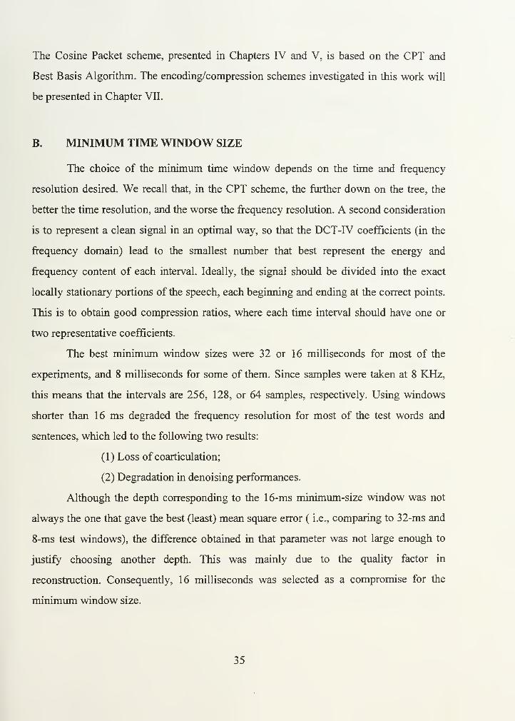
Figure 6.2 illustrates the short-time energy and zero-crossing plots (top) from

Voicedit, from the SPC Toolbox [16], for the sentence "/This place blows/" (bottom).

36

Figure 6.3 presents four plots. The first shows the time domain plot. The second and third

plots show, respectively, the frequency behavior according to Table 6.1, and the energy

behavior obtained by summing the squares of the coefficients in each interval. The fourth

plot (bottom) shows the spectrogram of the speech signal. Note that the tendency of both

frequency and energy plots match those of Figure 6.2.

Voiced-unvoiced segmentation obtained the best results when all the intervals

with the largest coefficient positioned at a frequency below 1 ,000 Hz, and energy above a

certain threshold were assigned as voiced. All the intervals with the largest coefficient at

a frequency above 1,000 Hz were assigned as unvoiced. Figure 6.3 illustrates that a

voiced sound results in a high energy and low frequency (largest coefficient frequency

below 1 ,000 Hz) representation for those segments. This is the case for the sounds "///,"

"/a/, " and "lo/. " In turn, unvoiced sounds are recognized as segments with high

frequency (largest coefficient frequency above 1 ,000 Hz) and low energy content. This is

the case of the sounds "Is/ " from "this" and "place." Figure 6.4 shows the result of the

voiced-unvoiced segmentation scheme, which can be observed in the middle plot. The

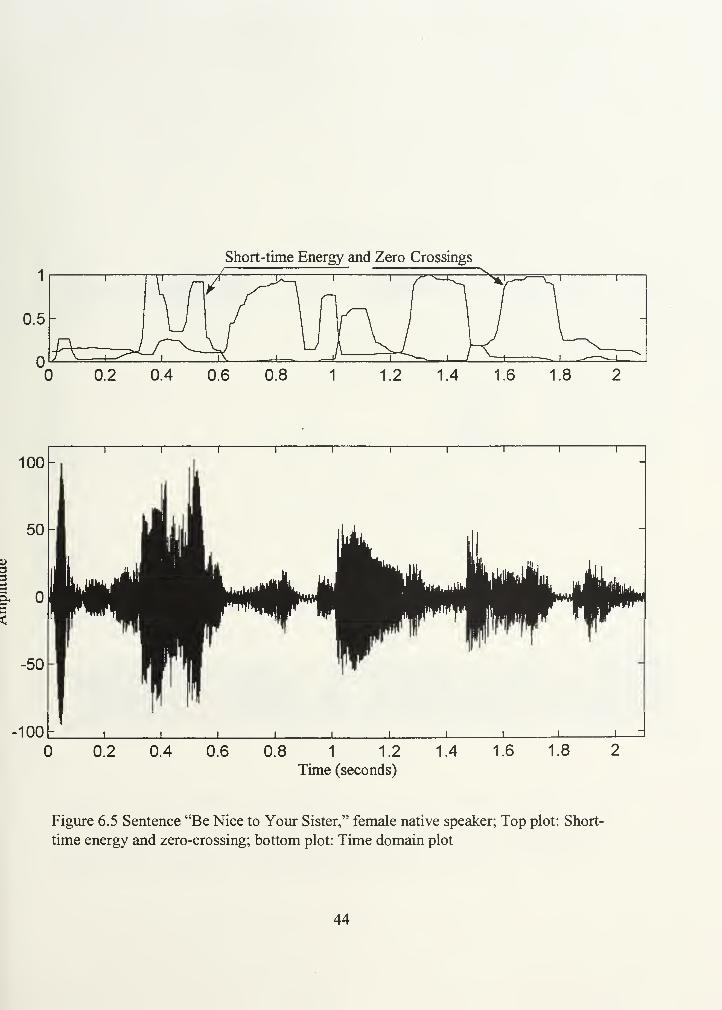
bottom plot contains the corresponding spectrogram. Figures 6.5, 6.6, and 6.7 present the

same kind of plots for the sentence "Be nice to your sister." Again, the voiced sounds

"lal/, " "/o/, " and "///" are distinguishable from the unvoiced "Is/, " and "///."

D. ADAPTIVE THRESHOLDING

This section utilizes the partitioning of speech into voiced-unvoiced segments to

implement an adaptive scheme for selecting cosine packet coefficients.

Experiments showed that a more natural sounding speech was reconstructed after

compression when using more coefficients to represent voiced than unvoiced segments.

This resulted in the use of a different percentage of coefficients in the following four

cases:

A) Low frequencies, low energy

37

B) Low frequencies, high energy

C) High frequencies, low energy

D) High frequencies, high energy.

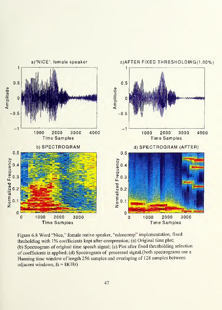
The need to select more coefficients to represent the voiced segments of speech is

illustrated in the example where the isolated noise-free word "nice" is compressed. As

explained in Section B, the minimum window size chosen is 16 ms. Figure 6.8 shows

that, when the compression scheme is set to keep one cosine packet coefficient per 1 6 ms

window to represent the phoneme /if, the higher formants of that phoneme are lost. As a

result, the phoneme lil tends to sound like a /u/. This example illustrates the fact that

more than one coefficient may be required to represent voiced phonemes accurately.

Figure 6.9 presents the plots that result when two CP coefficients per 16 ms window are

selected to represent voiced phonemes (including phoneme /if), and one CP coefficient

out of every 16 or 32 ms interval is selected to represent unvoiced phonemes. Although a

lower mean value is achieved for the percentage of selection (and, thus, a higher

compression rate), the sound HI is correctly reconstructed without affecting the other

phonemes of the word "nice."

Similar findings were obtained with other voiced phonemes such as /a/ and lol. In

addition, experiments showed that the voiced plosive /p/ was degraded by the

compression process and sounded like a Ibl. Keeping three cosine packet coefficients per

1 6 ms window interval for voiced segments led to a more accurate representation of the

information after compression, as confirmed by the smaller MSE and better sound quality

in the reconstructed signal. Further experiments showed that one cosine packet

coefficient per 16 ms interval is sufficient to represent the unvoiced segments accurately.

E. DENOISING

Previous sections have considered only the problem of compressing noise-free

signals. However, some of our recordings had a significant amount of low frequency

38

equipment noise located around 60 Hz and some of its harmonics. As a result, a denoising

step was investigated prior to compressing the data to improve the quality of the

compressed signal. Thus, the noisy speech signal was denoised prior to applying the

compression scheme. The denoising code is given in the Appendix.

Two different cases where noise was present were considered: Noise-only data

segments and noisy speech segments. Noise-only data segments occur before and after

isolated word recordings, and between words in the sentence recordings. Experiments

showed that the cosine packet coefficients allowed the detection of noise-only segments.

The following two situations characterizes the noise-only case according to

implementation ndencomp.m, given in the Appendix:

(1) Whenever the largest coefficient in the segment is at a frequency less

than or equal to 62.5 Hz, and the second largest coefficient is at a frequency less than or

equal to 300 Hz or higher than 1,000 Hz;

(2) Whenever the largest coefficient in the segment is in a frequency range

between 62.5 Hz and 250 Hz, and the second coefficient is at a frequency less than 200

Hz.

The following situations characterizes the noise-only case according to imple-

mentation encp6.m, given in the Appendix:

(1) The largest coefficient in the segment is at a frequency less than or

equal to 125 Hz, and the second largest coefficient is at a frequency less than 300 Hz;

(2) The largest coefficient is at a frequency less than 62.5 Hz, and the

second coefficient is at a frequency higher than 1 ,000 Hz;

(3) The largest coefficient is at a frequency less than 500 Hz for the female

speaker, or less than 1,000 Hz for the male speaker, and the second coefficient is at a

frequency less than 125 Hz.

All remaining cases are considered as noisy speech. For those cases, all

coefficients located at frequencies below or equal to 62.5 Hz are zeroed out.

Three specific noise-and-speech cases are presented as follows:

39

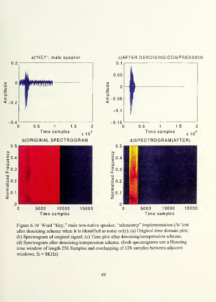
(1) Noisy speech-Case 1. An example of this case is the word "hey,"

where the sound /h/ was lost in the background noise. Due to the higher frequency

content of "/h/" (as opposed to the noise), it was possible to identify and pick up one

more CP coefficient per interval; thus, retrieving the sound of "/h/." This example is

illustrated in Figures 6.10 and 6.11, which show time plots and spectrograms that

correspond to keeping 1 CP and 2 CP coefficients/ 16- ms interval, respectively.

(2) Noisy speech-Case 2. This problem required differentiation of the

noise-only case from the noisy voiced stops lb/ and lp/. Distinguishing these sounds from

noise was easier than case 1 above, since the first largest coefficient obtained for those

two phonemes was never less than 250 Hz, making it possible to denoise without

interfering with those sounds.

(3) Noisy speech-Case 3. There were difficulties in separating the weak

ending Isl, such as in "cats" and "let's, from the background noise." Whenever this case

occurred, the Best Basis Algorithm produced a 32 ms time window with the first two

largest coefficients at frequencies less than 125 Hz. Although the phoneme "/s/" is

located at frequencies higher than 125 Hz, its energy was too small to be differentiated

from that of the noise. Thus, the data contained in the phoneme Isl is identified as noise

only and disregarded before the compression step. Figure 6.12 illustrates this case.

40

Short-time Energy and Zero-Crossings

0.2 0.4 0.6 0.8 1 1.2 1.4 1.6 1.8 2

100-

100-

0.8 1 1.2

Time (seconds)

Figure 6.2 Sentence "This Place Blows," male native speaker; top plot: Short-time

energy, zero-crossing representation; bottom plot: Time domain representation, fs = 8

KHz

41

l_

JO

>*2o

SicrCD

"This place blows"

2000 4000 6000 8000 10000Time samples

Frequency Behavior

12000 14000 16000

-I 1 1 1 1 1 i i

. I, 1 1. 1 1 1 1 1 1 1 1 I i ll, I

1

lli.j lllllll ,11 1..1 Ih 1 III 1 i i hi mil il . in

2000 4000 6000 8000 10000Time samples

Energy of Cosine Packet Coefficients

12000 14000 16000

2000 4000 6000 8000 10000 12000 14000 16000

Spectrogram

u,Vf -

2000 4000 6000 8000 10000Time samples

12000 14000 16000

Figure 6.3 Sentence "This Place Blows," male native speaker, "compcp" implementation;

(a) Time domain plot; (b) Frequency behavior plot according to Table 6. 1 ;(c) Energy

plot; (d) Spectrogram, using a Harming time window of length 256 samples and

overlapping of 128 samples between adjacent windows, fs = 8 KHz

42

"aCD

oo>c=»

I

T3<u

oo>

.5-

"This place blows"

2000 4000 6000 8000 10000

Time samples

Voiced-Unvoiced Segmentation

12000 14000 16000

. i llll 1 1 III . Lu_LL 11 JJ i _ J i iJL I I I 1 1 1 1 1

J

L_LL

2000 4000 6000 8000 10000

Time samples

Spectrogram

12000 14000 16000

2000 4000 6000 8000 10000Time samples

12000 14000 16000

Figure 6.4 Sentence "This Place Blows," male native speaker, "compcp" implementation;

(a) Time domain plot; (b) Voiced-unvoiced segmentation; (c) Spectrogram, using a

Harming time window of length 256 samples and overlapping of 128 samples between

adjacent windows, fs = 8 KHz

43

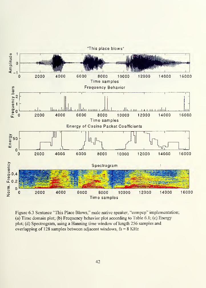
Short-time Energy and Zero Crossings

0.5-

0.2 0.4 0.6 0.8 1 1.2 1.4 1.6 1.8

100-

3.

100 b

Figure 6.5 Sentence "Be Nice to Your Sister," female native speaker; Top plot: Short-

time energy and zero-crossing; bottom plot: Time domain plot

44

a

>,2o

11

lo

"Be nice to your sister'

2000 4000 6000 8000 10000Time samples

Frequency Behavior

12000 14000

2000 4000 6000 8000 10000 12000Time samples

Energy of Cosine Packet Coefficients

14000

2000 4000

=3

cr 0.4

: 0.2

6000 8000 10000Time samples

Spectrogram

12000 14000

16000

1

II III 1 1 1 II III

1

II ,1 1 . 1

1

1 1. 1

1 1

III 1 1 1

1

Hull i

!

I

1

,111.1

16000

16000

2000 4000 6000 8000 10000

Time samples

12000 14000 16000

Figure 6.6 Sentence "Be Nice to Your Sister," female native speaker, "compcp"implementation; (a) Time domain plot; (b) Frequency behavior plot, according to Table

6.1; (c) Energy plot; (d) Spectrogram, using a Harming time window of length 256samples and overlapping of 128 samples between adjacent windows, fs = 8 KHz

45

"°1

a>

oo>

^0.5-ad>o

1

ocCD

ST 0-4CD

2000

"Be nice to your sister"

4000 6000 8000 10000

Time samples

Voiced-Unvoiced Segmentation

12000 14000

2000 4000 6000 8000 10000Time samples

Spectrogram

12000

16000

14000 16000

oZ 2000 4000 6000 8000 10000

Time samples

12000 14000 16000

Figure 6.7 Sentence "Be Nice to Your Sister," female native speaker, "compcp"

implementation; (a) Time domain plot; (b) Voiced-unvoiced segmentation;

(c) Spectrogram, using a Harming time window of length 256 samples and overlapping

of 128 samples between adjacent windows, fs = 8KHz

46

a)"NICE", female speaker

0.5

T3

E<

-•0.5

0.5

oSo

2o-a

|0

loZ

1000 2000 3000Time Samples

b) SPECTROGRAM

4000

"£R§2SS6G£^™™w

1 vfisy".'",^.

HwW1'"^"— ^^^^p3^w

" $LHD8E^5^~if«Ki4

',

ifel^1$

UJfU

F^l^ff*>

j-.-i ..-_.—H^ffrSSiisu •.«...'

1000 2000 3000Time Samples

c)AFTER FIXED THRESHOLDING^ .00%)

1

oT3

*—'

"a.

E<

-0.5

1000 2000 3000 4000Time Samples

d) SPECTROGRAM (AFTER)

1000 2000 3000

Time Samples

Figure 6.8 Word "Nice," female native speaker, "ndencomp" implementation, fixed

threholding with 1% coefficients kept after compression; (a) Original time plot;

(b) Spectrogram of original time speech signal; (c) Plot after fixed thresholding selection

of coefficients is applied; (d) Spectrogram of processed signal.(both spectrograms use a

Harming time window of length 256 samples and overlaping of 128 samples between

adjacent windows, fs = 8KHz)

47

a)"NICE", female speaker

a)

XJ=j

"5.

E<

-0.5

1000 2000 3000Time Samples

b) SPECTROGRAM

4000

1000 2000 3000Time Samples

c)AFTER ADAPTIVE THRESHOLDING^.98%1

0)

a

"a.

E<

1000 2000 3000 4000Time Samples

d) SPECTROGRAM (AFTER;

1000 2000 3000

Time Samples

Figure 6.9 Word "Nice," female native speaker, "ndencomp" implementation, adaptive

thresholding, with an average of 0.98% CP coefficients kept for compression; (a) Original

time domain plot; (b) Spectrogram of original speech signal; (c) Time domain plot of

processed signal; (d) Spectrogram of processed signal.(both spectrograms use a Harming

time window of length 256 samples and overlaping of 128 Samples between adjacent

windows, fs = 8 KHz)

48

a)"HEY", male speaker

0.5 1 1.5

Time samples -

n'

b)ORIGINAL SPECTROGRAM

5000 10000Time samples

15000

c)AFTER DENOISING/COMPRESSION0.1

-0.150.5 1 1.5

Time samples . _'

d)SPECTROG RAM (AFTER)

5000 10000

Time samples

15000

Figure 6.10 Word "Hey," male non-native speaker, "ndencomp" implementation (/h/ lost

after denoising scheme when it is identified as noise only); (a) Original time domain plot;

(b) Spectrogram of original signal; (c) Time plot after denoising/compression scheme;

(d) Spectrogram after denoising/compression scheme, (both spectrograms use a Harming

time window of length 256 Samples and overlapping of 128 samples between adjacent

windows, fs = 8KHz)

49

a)"HEY", male speaker

0.5 1 1.5

Time samples , n<

A I U

b)ORIGINAL SPECTROGRAM

5000 10000Time samples

15000

c)AFTER DENOISING/COMPRESSION0.1

-0.15

0.5

0.5 1 1.5

Time samples „ , „'x i u

d)SPECTROGR AM (AFTER)

5000 10000

Time samples

15000

Figure 6.1 1 Word "Hey," male non-native speaker, "ndencomp" implementation (/h/

recovered after denoising scheme when it is identified as a noisy speech); (a) Original

time domain plot; (b) Spectrogram after denoising/compression scheme; (c) Time plot

after denoising/compression scheme;(both spectrograms use a Hanning time window of

length 256 and overlaping of 128 samples between adjacent windows, fs = 8 KHz)

50

a)"CATS", female speaker

5000Time samples

10000

b)ORIGINAL SPECTROGRAM

2000 4000 6000Time samples

8000

c)AFTER DENOISING/COMPRESSION1

CD

=3

"q.

E<

5000 10000Time samples

d)SPECTROGR AM (AFTER)

2000 4000 6000

Time samples

8000

Figure 6.12 Word "Cats," female non-native speaker, "ndencomp" implementation {Isi

lost after denoising scheme when it is identified as noise only); (a) Original time domain

plot; (b) Spectrogram of original speech; (c) Time domain plot after denoising /

compression; (d) Spectrogram after denoising/compression (both spectrograms use a

Harming time window of length 256 and overlapping of 128 samples between adjacent

windows, fs = 8 KHz)

51

52

VII. ENCODING SCHEMES

This chapter is divided into three main sections. The first proposes a quantization

scheme to transmit the CP coefficients. The second proposes encoding schemes to

transmit the side information, i.e., both the locations and the initial indexes of each

segment. The third section presents the coding scheme used to transmit the coefficients

vector, the locations vector and the vector containing the initial locations of each

segment.

A. THE QUANTIZATION SCHEME

Once data is available for transmission, the user must quantize and code it. After

the compression scheme proves to be efficient, and allows a good quality reconstruction,

consideration is given to finding a uniform quantizer that can reproduce efficiently the

coefficients to be transmitted [14].

Three different vectors must be sent for speech compression. The first vector

contains the cosine packet coefficients. The second contains the location of the

coefficients. The third vector contains the initial time locations of each segment. To

transmit the first vector, i.e., the coefficients vector, the following is done:

(1) The data are normalized by dividing all the vectors by the maximum

absolute value of all the coefficients. This value turns out to be the scaling factor;

(2) The whole vector is multiplied by QL/2 (where QL is the number of

quantizing levels selected by the user), and rounded to the closest integer.

By performing these steps, a QL-level quantizer is built. It has QL levels due to

the normalization and further multiplication by QL/2, which assures that the positive and

negative parts of speech will be always between -QL/2 and +QL/2.

(3) The scaling factor, equal to maximum absolute value of all the

coefficients, is sent. In the receiver the following steps are to be performed:

(a) Upon receiving the vector, divide it by QL/2, recovering the

rounded normalized coefficients vector;

53

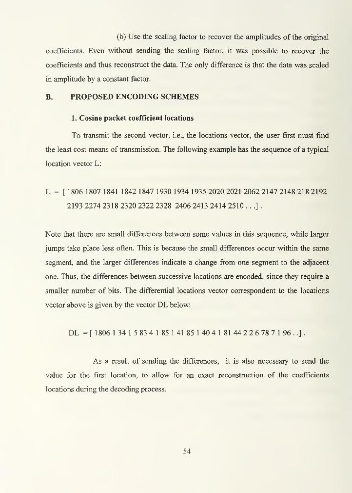
(b) Use the scaling factor to recover the amplitudes of the original

coefficients. Even without sending the scaling factor, it was possible to recover the

coefficients and thus reconstruct the data. The only difference is that the data was scaled

in amplitude by a constant factor.

B. PROPOSED ENCODING SCHEMES

1. Cosine packet coefficient locations

To transmit the second vector, i.e., the locations vector, the user first must find

the least cost means of transmission. The following example has the sequence of a typical

location vector L:

L =[ 1806 1807 1841 1842 1847 1930 1934 1935 2020 2021 2062 2147 2148 218 2192

2193 2274 2318 2320 2322 2328 2406 2413 2414 2510 . . .]

.

Note that there are small differences between some values in this sequence, while larger

jumps take place less often. This is because the small differences occur within the same

segment, and the larger differences indicate a change from one segment to the adjacent

one. Thus, the differences between successive locations are encoded, since they require a

smaller number of bits. The differential locations vector correspondent to the locations

vector above is given by the vector DL below:

DL =[ 1806 1 34 1 5 83 4 1 85 1 41 85 1 40 4 1 81 44 2 2 6 78 7 1 96 . .]

.

As a result of sending the differences, it is also necessary to send the

value for the first location, to allow for an exact reconstruction of the coefficients

locations during the decoding process.

54

2. Segment Indexes

The third vector to transmit is the vector that corresponds to the indexes of each

segment. The Best Basis Algorithm selects the basis by searching for the minimum

entropy representation. When the length of each new window is obtained, the algorithm

outputs the two parameters "b" and "d," which allow the beginning index of the next time

window to be computed. The expression for obtaining index "i" is as follows:

' = £•»+!> (7-1)

where n is the original length of each window. Since the parameters "b" and "d" are small

numbers, composed of one or two digits and, therefore, much smaller than the indexes

themselves, it is a good idea to transmit the parameters instead of the indexes. Thus, the

two vectors "nde" and "nbe," which are composed of the parameters "b" and "d" of each

time window, are transmitted. For example, suppose the vectors nde and nbe are given as

follows:

nde = [4665566566554423665].

nbe = [045 3 4 10 11 6 14 15 9 10 11 6726 5657].

Considering n = 8192 time samples, the corresponding vector I containing the

initial locations of the first eight segments is given by :

I = [ 1 512 640 768 1024 1280 1408 1536 ...]

.

To reconstruct the locations vector of the non-zero coefficients, the receiver works

on the received vector of differential locations DL and reconstructs L. The reconstructed

vector is then called RL.

Once the locations of non zero coefficients (vector RL) are available, along with

the locations of the beginning of each new segment (vector I), the receiver will be able to

apply the DCT transform to reconstruct the speech signal.

55

C. CODING SCHEMES

After quantization, the coefficients vector is encoded using Huffman Coding

[14], which minimizes the total number of bits by assigning more bits to less frequent

symbols and less bits to more frequent ones. The vectors nde and nbe are transformed

into only one vector and passed through the Huffman Coder. The inputs include the

number of symbols and the probabilities of each one, whereas the outputs from the

Huffman Coder are the coded words and average length of the symbols. In order to

perform the quantization step and also compute the probabilities of occurrences of each

symbol to be coded, the function quantx.m, given in the Appendix, was implemented.

That function receives the original vector, the number of levels desired for quantization,

and returns the quantized vector and the probabilities in descending order, as required by

the Huffman Coder (the Huffman Coder used is given in the Appendix). The code was

adapted as a function to be called whenever this step is necessary. Finally, the exact

number of bits necessary to encode the differential locations vector (DL) is computed.

56

VIII. TESTS AND RESULTS

A. INTRODUCTION

This chapter describes the procedures that are used to test the compression and

encoding schemes. First, the basic compression scheme results are presented. Next, the

combined denoising/compression schemes are given. Then, encoding performances,

which are used to transmit the compressed information, are presented. Finally, the Cosine

Packet compression scheme performances are compared with those obtained using the the

related Wavelet Packet Transform.

B. COMPRESSION SCHEME RESULTS

The compression-only scheme is first applied to "clean" speech to evaluate its

performance. To test this scheme on isolated words, we use the words "project,"

"cataratas," and the segment "encyclope," extracted from the word encyclopedia. This

compression scheme is also implemented in the following two sentences:

" Be nice to your sister," spoken by a female native speaker; and

" This place blows," spoken by a male native speaker.

1. Description

The testing software requires the user to input the following:

(1) The gender of the speaker. This information is required since the pitch

for a female speaker occurs at a higher frequency than that of a male speaker;

(2) Word or sentence to be compressed;

(3) Maximum depth used for the cosine packet time splitting, which in

turns fixes the minimum size of the window;

The following outputs are provided:

(1) The mean square error between the original and the reconstructed

speech signal;

57

(2) The number of non-zero cosine packet coefficients in the original

signal (ONCOEF);

(3) The number of non-zero cosine packet coefficients selected by the

compression scheme (FNCOEF);

(4) The reconstructed speech signal obtained after compression.

Two different compression implementations were considered, which differ in the

number of cosine packet coefficients kept to compress the speech signal. The first

compression scheme (implemented in compcp.m, given in the Appendix) selects the

cosine packet coefficients as follows:

(1) Keep the top 0.5% non-zero coefficients (rounded to the closest

integer) in each time window when the speech segment is detected as unvoiced; this

percentage means selecting one coefficient out of every interval containing 128

coefficients, one coefficient out of every interval containing 256 coefficients, and so on,

according to the result of the rounding process;

(2) Keep the top 1.3% non-zero coefficients (rounded to the closest

integer) for each time window of minimum length (16 ms) when the speech segment is

identified as voiced; this means selecting two coefficients out of every 128 coefficients,

three coefficients out of every interval containing 256 coefficients, and so on;

(3) Keep the top 2.34% non-zero coefficients (rounded to the closest

integer) for each time window larger than 16 ms when the speech segment is identified as

voiced; this means selecting three coefficients out of every interval containing 128

coefficients, six coefficients out of every interval containing 256 coefficients, and so on.

The second compression scheme (implemented in necompcp.m and given in the

Appendix) uses the following schemes to compress the speech signal:

(1) Keep the top 0.5% non-zero coefficients (rounded to the closest

integer) in each time window when the speech segment is unvoiced; this means selecting

one coefficient out of every interval containing 128 coefficients, one coefficient out of

every interval containing 256 coefficients, and so on;

58

(2) Keep the top 1.3% non-zero coefficients (rounded to the closest

integer) for each time window when the speech segment is identified as voiced; this

means selecting two coefficients out of every interval containing 128 coefficients, three

coefficients out of every interval containing 256 coefficients, and so on.

2. Experimental Results

Results obtained for the two compression schemes are presented in Table 8.2. In

Chapter VI, Figures 6.8 and 6.9 present time domain plots and spectrograms for the

Adaptive Thresholding compression scheme considered in this section. The parameters

used to measure degradation due to the compression scheme are:

(1) The mean square error (MSE) between the original and the reconstructed

speech signal;

(2) A subjective evaluation made by five different users of the quality of the

reconstructed signal when compared to the quality of the original signal. The evaluation

was graded on a scale from 1 to 5, according to Table 8.1.

GRADE Speech Quality Level of Distortion

5 Excellent Imperceptible

4 Good Just perceptible but not annoying

3 Fair Perceptible and slightly annoying

2 Poor Annoying but not objectionable

1 Unsatisfactory Very annoying and objectionable

Table 8. 1 Mean opinion score table

(3) The ratio between the number of non-zero cosine-packet coefficients kept after

compression and the total number of initial non-zero coefficients obtained with the cosine

packet decomposition (ONCOEF/FCOEF%).

59

3. Comments

Note the slightly higher speech quality mean grades assigned to code compcp.m,

which also presents a slightly higher percentage of coefficients kept (i.e., a lower

compression ratio). Experiments showed that fixed thresholding selects 1% of the set of

coefficients, and leads to the distortion of voiced phonemes (e.g., I'll ends up sounding

like /u/ in the word "nice"). The "after compression" spectrogram included in the bottom

right of Figure 6.8 showed that the higher formant section of the phoneme l\l has not been

preserved in the compression. By comparison, Figure 6.9 showed the results obtained

using an adaptive thresholding scheme, which selects more coefficients for the voiced

segments while keeping a smaller total percentage of coefficients (0.98%). The after-

compression spectrogram shown in Figure 8.2 shows that the high formants of the

phoneme /if are better preserved, leading to a better reconstruction of the voiced

phoneme.

60

"Be "This

Parameters "Project" "Cataratas" "Encyclope" "Issos" "Assos" Nice" Place"

Code: NECOMP.M

MSE 0.0045 0.0315 0.0127 0.0074 0.0136 0.0070 0.0432

ONCOEF 8192 8192 8192 8192 8192 16384 16384

FNCOEF 124 100 104 100 100 210 216

% 1.51 1.22 1.27 1.22 1.22 1.28 1.32

ONCOEF/

FNCOEF.

Speechquality

2.2 2.4 2.8 2.8 2.2 3.2 3.0

mean grade

Code: COMPCP.M

MSE 0.0038 0.0313 0.0121 0.0057 0.0115 0.005

2

0.029

7

ONCOEF 8192 8192 8192 8192 8192 16384 16384

(original #of

coeff>0)

FNCOEF 181 109 126 129 115 139 228

(final # of

coeff. X))

% 2.21 1.33 1.54 1.57 1.40 0.85 1.39

ONCOEF/

FNCOEF

Speechquality

2.6 2.6 2.8 3.0 2.2 3.4 3.2

mean grade

Table 8.2 Compression only results

61

C. DENOISING-COMPRESSION RESULTS

1. Description

Next, we consider the application of a combined denoising and compression

scheme designed to minimize the effects ofnarrowband equipment noise in a few isolated

words and sentences. The isolated words used in these tests are:

"Be", spoken by a female and by a male speaker;

"Cats", spoken by a female speaker;

"Hey", spoken by a female and by a male speaker;

"Met", spoken by a female speaker; and

"Pay", spoken by a female speaker.

The sentences used are:

"Hello, my name is Roberto, today is Tuesday;" and

"Bye, guys, I'm going back to Brazil", both spoken by a male speaker.

Two different implementations for the denoising scheme are considered: The first

is implemented in ndencomp.m and the second is implemented in encp6.m (both are

listed in the Appendix). The noise identification and denoising process for each

implementation can be found in Chapter VI, Section E, and in the Appendix. Details

regarding the compression scheme for both implementations can be found in the

Appendix. Table 8.3 presents the compression results for tests applied on the same

"clean" words of the previous section, but using the codes ndencomp.m and encp6.m.

2. Results

The parameters used to evaluate the denoising/compression scheme are identical

to those defined for the compression-only scheme, with the exception of the mean square

error (MSE). This parameter was omitted because the denoising step produced a greater

difference between the original and the reconstructed signals. The performance results are

presented in Table 8.4.

62

Parameters "Project" "Cataratas" "Encyclope" "Issos" "Assos"

"Be

Nice"

"This

Place"

Code: NDENCOMP.M

ONCOEF 8192 8192 8192 8192 8192 16384 16384

FNCOEF 189 153 152 129 145 277 224

%

ONCOEF/

FNCOEF

2.31 1.87 1.86 1.87 1.77 1.69 1.37

Speech quality

mean grade

2.5 3.0 3.0 3.2 2.6 3.3 3.2

Code: ENCP6.M

ONCOEF 8192 8192 8192 8192 8192 16384 16384

FNCOEF 188 149 152 129 143 270 264

%

ONCOEF/

FNCOEF

2.29 1.82 1.86 1.86 1.75 1.65 1.61

Speech quality

mean grade

2.5 3.3 3.2 3.4 2.8 3.5 3.4

Table 8.3 Compression results utilizing codes ndencomp.m and encp6.m

The speech quality mean grade was computed for the following speech data: The

words "Be," female speaker, and "pay," male speaker, and the sentences "Hello, my name

is Roberto ..." and "Bye, guys, I'm going back ..." These results are presented in Table

8.5.

63

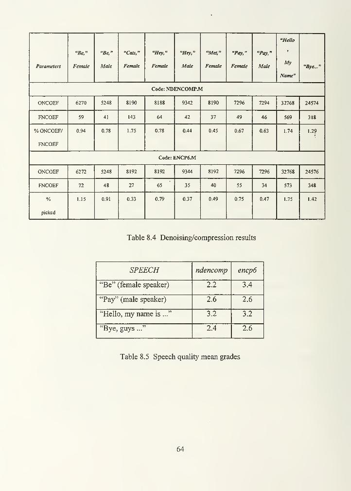
Parameters

"Be,"

Female

"Be,"

Male

"Cats,"

Female

"Hey,"

Female

"Hey,"

Male

"Met,"

Female

"Pay,"

Female

"Pay,"

Male

"Hello

My

Name"

"Bye..."

Code: NDENCOMP.M

ONCOEF 6270 5248 8190 8188 9342 8190 7296 7294 32768 24574

FNCOEF 59 41 143 64 42 37 49 46 569 318

% ONCOEF/

FNCOEF

0.94 0.78 1.75 0.78 0.44 0.45 0.67 0.63 1.74 1.29

Code: ENCP6.M

ONCOEF 6272 5248 8192 8192 9344 8192 7296 7296 32768 24576

FNCOEF 72 48 27 65 35 40 55 34 573 348

%

picked

1.15 0.91 0.33 0.79 0.37 0.49 0.75 0.47 1.75 1.42

Table 8.4 Denoising/compression results

SPEECH ndencomp encp6

"Be" (female speaker) 2.2 3.4

"Pay" (male speaker) 2.6 2.6

"Hello, my name is ..." 3.2 3.2

"Bye, guys ..." 2.4 2.6

Table 8.5 Speech quality mean grades

64

3. Comments

We note that the overall speech quality mean grades in Table 8.3 are slightly

increased when compared to those from Table 8.2. We also note that the

ONCOEF/FNCOEF percentages in Table 8.4 are small, since large sections of data are

identified as noise-only. Thus they are not retained for compression by the denoising step.

Results obtained for both denoising/compression schemes show slightly better speech

quality for the encp6.m implementation than for the ndencomp.m implementation.

a. Word "be"

Both denoising/compression schemes produce good results for the word "be"

for male and female speakers. The plots in Figure 8.1 show the efficiency of the

algorithm in both the time and frequency domain. The quality of the reconstructed speech

is good, as illustrated by the grades assigned by five native listeners.

b. Word "Hey"

For male and female cases, both denoising/compression schemes produce

good results (Figures 8.2 and 8.3). The quality of the reconstructed speech is high, as

confirmed by the listening tests. Note that the /h/ sound in the female speech has a higher

frequency than that of the male voice. The denoising schemes also allow the phoneme /h/

to be differentiated from the noisy background environment.

d. Word "met"

Both denoising/compression schemes produce a good reconstruction of

"/me/" and a poor reconstruction of the phoneme Ixl, which is reconstructed sounding like

a "/dV." This degradation is due to the combination of too few coefficients kept for

compression in this section of the word and a noisy background.

65

e. Word "Pay"

The reconstructed sound quality is better for the male case (Figures 8.4 and

8.5). Again, this was due to too few coefficients being kept. The sound /p/ has its first two

largest CP coefficients below 400 Hz and around 1,000 Hz, respectively. Higher energy is

concentrated in the lower frequency coefficients. When spoken by a female, the higher

frequency coefficients get less energy compared to others not so important from the lower

frequency portion. For that reason, fewer coefficients from the higher frequency portion

are kept, leading to a poorer sound than the male version.

/ Sentence "Hello, my name is Roberto, today is Tuesday"

The spectrograms in Figure 8.6 show that the main signal energy is preserved,

and that denoising occurs in the correct time intervals.

g. Sentence " Bye, guys, I'm going back to Brazil"

For this sentence, both denoising-plus-compression schemes result in a good

reconstruction. It is possible to observe in the spectrograms of Figure 8.7 that the

algorithm picks up the important cosine packet coefficients. In this case, no significant

amount of denoising was done due to the high quality of the original speech. However, it

is worth comparing the effects of the denoising schemes. Note that, in using ndencomp.m

the resultant signal is divided more by noisy intervals than when using encp6. In the

listening tests for both sentences, the mean grade assigned to the reconstruction using

ndencomp.m is better than the one assigned when using encp6.m. Basically, the unvoiced

sounds had a better reconstruction using the former code, whereas the latter code

produced some distortion, leading to what was called a mechanical sound by some

listeners.

66

D. ENCODING SCHEMES RESULTS

1. Description

The data used for these tests consist of twelve speech sequences of lengths 8 1 92

(ten words and/or sounds), 32768 (one sentence) and 65536 (one dialogue). The software

used for this set of tests includes voiced-unvoiced segmentation, denoising, compression,

and encoding steps. Both denoising/compression schemes are used in these tests. The

coding software is presented in the Appendix. The minimum window size is 16

miliseconds. The compression ratio between the total number of bits after encoding and

the total original number of bits, is used to evaluate the performance of the encoding

scheme. The original number of bits is computed by multiplying the number of bits used

to represent each incoming sample (the samples had 8 bits and were PCM compressed)

by the original number of samples. For example, for each of the ten sequences of length

8192, the original number of bits is 8192-8 = 65,536 bits per speech sequence. The

following speech sequences are used in our tests:

(a) "BE," spoken by a female speaker;

(b) "HEY," spoken by a female speaker;

(c) "MET," spoken by a female speaker;

(d) "PAY," spoken by a female speaker;

(e) "CATS," spoken by a female speaker;

(f) Word "PROJECT," spoken by a male speaker;

(g) Word "CATARATAS," spoken by a male speaker;

(h) Sound or partial word "ENCYCLOPE", spoken by a male speaker;

(i) Sound "ASSOS," spoken by a male speaker;

(j) Sound "ISSOS," spoken by a male speaker;

(k) Sentence "Bye guys, I'm going back to Brazil," male speaker;

(1) Dialogue from a telephone conversation, male and female speakers.

67

2. Results

A measure of distortion is obtained by comparing the quality between the original

speech signal and the reconstructed signal. ("Speech quality" in Table 8.1).

To evaluate the efficiency of the encoding scheme, the following

parameters are chosen:

(1) The COMPRATIO, defined as one minus the ratio between the total

number of bits after compression and the total number of bits in the original signal;

(2) The mean square value of the quantization error.

The performance results for the encoding scheme are presented in the Table 8.6.

All results are based on the denoising/compression implementation ndencomp.m, except

for the words "hey" and "met," which use encp6.m.

SPEECH SPEECH

QUAL

MSECOMPRATIO

%

"Be" 2.6 98.70% 5.12e"7

"Hey" 3.2 98.56% 9.32e"6

"Met" 3.2 98.85% S^e"6

"Pay" 3.0 99.17% 5.22e"7

"Cats" 3.4 98.59% l.Ole"5

"Project" 3.2 97.87% 1.06e"5

"Cataratas" 3.4 97.65% 4.6 le"5

"Encyclope" 3.8 97.64% 2.86c"4

"Assos" 3.2 97.87% 3.62e'5

"Issos" 4.0 98.05% 2.16e"5

"Bye, guys..." 2.4 98.10% 2.707e"5

Tel. conversation 2.6 98.06% 2.843e"5

Table 8.6 Encoding results, 64-level quantizer.

68

The mean speech quality grade assigned is 3.2 (see MOS Table 8.1). This means

perceptible and slightly annoying. We also note the high values of compression ratios and

the very small values of MSE, which corresponds to the mean square quantization error.

The compression ratio is calculated in the following way. Eight bits are used for

each original sample of data, since that is the number used to load speech recordings into

"Matlab." The total number of bits is computed by multiplying each average number

from the Huffman coder by the corresponding number of samples in the coefficients

vector, as well as in the three vectors used to transmit the locations and the window

boundaries. The compression ratio is then computed as the ratio between the final total

number of bits and the original total mumber of bits after the encoding process.

Comparing the percentages from this encoding table to the ones from the previous

sections(compression and denoising/compression), we note that, although still very low,

the numbers from the encoding process are higher ( ~ 2%) in comparison to the others (~

0.85%). The reason is that, in addition to the cosine packet coefficients, the side

information (i.e., the locations of those coefficients) must also be encoded. Thus, even

though the number of bits is reduced due to the quantization process, the increase of

information to be transmitted makes the number a little higher.

As can be noted from the grades assigned, the encoding process results are good.

The only problem are the low-energy coefficients corresponding to unvoiced sounds

when submitted to the quantization and rounding processes. Figure 8.8 shows the word

"project," which lost its weak, final DsXl. Even when we change the quantizer to 32 and 64

levels, it is still impossible to recover the final sound.

Figure 8.9 presents the sentence, "Be nice to your sister," using a 16-level

quantizer. We note that the sounds /s/ in "nice", Itl in "to," and III in "your" are lost.

However, when the quantizer is changed to 32 levels, the main parts of these sounds are

recovered (Figure 8.10). Finally, when the number of levels is increased to 64 (Figure

8.11), the sequence sound is totally reconstructed, and practically no difference is noted

between the original and reconstructed sounds.

69

Similar results are observed for the sentence, "Bye guys, I'm going back to

Brazil." The phoneme IzJ from "guys" is lost with a 16-level quantizer (Figure 8.12), and

is recovered with a 32-level quantizer (Figure 8.13). Similarly, when a 16-level quantizer

was applied, the sound /h/ in the word "hey" was reconstructed like a /k/, resulting in a

word sounding like "kay" (Figure 8.14). By changing to a 32-level quantizer, it was

possible to recover the correct sound (Figure 8.15). The sound was even better with a 64-

level quantizer (Figure 8.16). Note the sequential progress in the coefficients recovered in

Figures 8.14 through 8.16, by comparing the plots (d) and (f).

Two points are worth mentioning. First, after the number of quantizing levels is

doubled, the compression ratio does not decrease significantly. For example, for the word

"project" (with a higher SNR, an almost "clean" word), when the number of levels is

increased from 16 to 32 (i.e. changing from 4 to 5 bits/symbol), the compression

percentage changes from 98.36% (1:61.2) to 98.28% (1:58.4). Another example is the

word "hey" (also a high SNR). The three compression percentages corresponding to the

16-level, 32-level, and 64-level quantizers are, respectively, 99.23% (1:130.4), 99.16%

(1:119.2), and 99.11% (1:113.2), respectively. Thus, a 64-level quantizer is used as a

good compromise between quality and compression.

E. COMPARISON WITH WAVELET PACKET TRANSFORM

In this section, the Cosine Packet is compared to the Wavelet Packet-based

compression procedure in clean (high SNR) speech. A "clean"( high SNR) speech

sequence is chosen, and the results are compared up to only the compression scheme,

since the encoding scheme performs basically the same for both cases.

The sentence "Be nice to your sister" is compressed using the Cosine Packet

Transform, and the average percentage of non-zero coefficients selected from the original

number equals 0.85% for a good reconstruction of the speech. A much poorer

70

reconstruction results from the Wavelet Packet Transform using the "Daubechies(4)"

wavelet basis function. The WT is implemented using the same criteria as those defined

for the CPT implementation with the WaveLab Package [17].

The result obtained for this sentence can be analyzed through the time and

frequency plots for both schemes given in Figures 8.17 and 8.18. We note that, in the

Wavelet Packet Transform, there are "holes" in the time domain. We note also that those

"holes" happen to be exactly at the intervals where the energy is lower, i.e., mainly at the

unvoiced sounds. This is because the WPT scheme initially splits the signal into given

frequency windows. In our example, only the highest 15% coefficients for given

frequency ranges are selected during the whole period of time.

By comparison, the CPT splits the signal first in the time domain. Then, for each

time frame, a thresholding is applied for the cosine packet coefficients. As a result,

although many fewer coefficients are selected, there is no chance of having a time

interval not represented. Actually, in this scheme, the holes are in the frequency domain.

But, since the transform is good enough to detect the main frequencies contained in each

locally stationary portion of the signal, the few cosine packet coefficients preserved at

each time interval are sufficient to allow for a good reconstruction of the speech. These

results confirm the theoretical expectation of superiority of the CPT over the WPT for

speech signal compression applications.

71

a)"BE", male speaker

a4—

•

E<

-0.2

-0.45000

Time samples10000

b)ORIGINAL SPECTROGRAM

2000 4000 6000Time samples

8000

c)AFTER DENOISING/COMPRESSION0.2

-0.25000 10000

Time samples

d)SPECTROGR AM (AFTER)

2000 4000 6000

Time samples

8000

Figure 8.1 Word "Z?e," male non-native speaker, "ndencomp" implementation;

(a) Original time domain plot; (b) Spectrogram of original plot; (c) Time domain plot

after denoising/compression; (d) Spectrogram after denoising/compression (both

spectrograms use a Harming time window of length 256 samples and overlapping of 128

samples between adjacent windows, fs = 8 KHz)

72

a)"HEY", male speaker

-0.40.5 1 1.5

Time samples . n<K x 10

b)ORIGINAL SPECTROGRAM

5000 10000Time samples

15000

c)AFTER DENOISING/COMPRESSION0.1

-0 150.5 1 1.5

Time samples .n

<

d)SPECTROGR AM (AFTER)

5000 10000Time samples

15000

Figure 8.2 Word "Hey" male non-native speaker, "ndencomp" implementation;

(a) Original time domain plot;(b) Spectrogram of original speech; (c) Time domain plot

after denoising/compression; (d) Spectrogram after denoising/compression (both

spectrograms use a Harming time window of length 256 samples and overlapping of 128

samples between adjacent windows,fs = 8 KHz)

73

a)"HEY", female speaker

5000Time samples

10000

b)ORIGINAL SPECTROGRAM

2000 4000 6000Time samples

8000

c)AFTER DENOISING/COMPRESSION0.5

5000 10000Time samples

d)SPECTROGR AM (AFTER)

2000 4000 6000Time samples

8000

Figure 8.3 Word "Hey" female non-native speaker, "ndencomp" implementation;

(a) Original time domain plot; (b) Spectrogram of original speech; (c) Time domain plot

after denoising/compression; (d) Spectrogram after denoising/compression (both

spectrograms use a Harming time window of length 256 samples and overlapping of 128

samples between adjacent windows, fs = 8 KHz)

74

a)"PAY", female speaker

a)

"a

a.

-0.5

5000Time samples

10000

b)ORIGINAL SPECTROGRAM

2000 4000 6000Time samples

8000

c)AFTER DENOISING/COMPRESSION0.6

-0.45000 10000

Time samples

d)SPECTROG RAM (AFTER)

2000 4000 6000

Time samples

8000

Figure 8.4 Word "Pay" female non-native speaker, "ndencomp" implementation;

(a) Original time domain plot; (b) Spectrogram of original speech; (c) Time domain plot

after denoising/compression; (d) Spectrogram after denoising/compression (both

spectrograms use a Harming time window of length 256 samples and overlapping of 128

samples between adjacent windows, fs = 8 KHz)

75

a)"PAY", male speaker

5000Time samples

10000

b)ORIGINAI_ SPECTROGRAM

2000 4000 6000Time samples

8000

c)AFTER DENOISING/COMPRESSION0.4

0)

a

"a.

E<

-0.2

-0.45000 10000

Time samples

d)SPECTROGR AM (AFTER)

2000 4000 6000

Time samples

8000

Figure 8.5 Word "Pay," male non-native speaker, "ndencomp" implementation;

(a) Original time domain plot; (b) Spectrogram of original speech; (c) Time domain plot

after denoising/compression; (d) Spectrogram after denoising/compression (both

spectrograms use a Harming time window of length 256 samples and overlapping of 128

samples between adjacent windows, fs = 8 KHz)

76

a)"Hello, my name is...", male speak

0.5

er c)AFTER DENOISING/COMPRESSION0.4

1 2 3

Time samplesx 10

b)ORIGINAL SPECTROGRAM0.5 . „ _, i

ftJiJi

1 2

Time samplesx 10

12 3 4

Time samples .

fi

4

d)SPECTROGR AM (AFTER)

Time samplesx 10

Figure 8.6 Sentence "Hello, my name is Roberto, today is Tuesday," male non-native

speaker, "ndencomp" implementation; (a) Original time domain plot; (b) Spectrogram of

original speech; (c) Time domain plot after denoising/compression; (d) Spectrogram after

denoising/compression(both spectrograms use a Harming time window of length 256

samples and overlapping of 128 samples between adjacent windows, fs = 8 KHz)

77

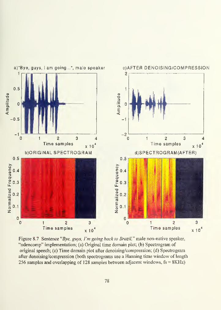
a)"Bye, guys, I am going...", male speaker

1 r-T-i

0)

T3

"5.

E<

-0.5

1 2 3

Time samples , _rx 1

b)ORIGINAL SPECTROGRAM

1 2

Time samplesx 10

c)AFTER DENOISING/COMPRESSION2

1 2 3

Time samples ,fi

d)SPECTROGR AM (AFTER)

1 2

Time samplesx 10

Figure 8.7 Sentence "Bye, guys, I'm going back to Brazil," male non-native speaker,

"ndencomp" implementation; (a) Original time domain plot; (b) Spectrogram of

original speech; (c) Time domain plot after denoising/compression; (d) Spectrogram

after denoising/compression (both spectrograms use a Harming time window of length

256 samples and overlapping of 128 samples between adjacent windows, fs = 8KHz)

78

a)Original "PROJECT"

CD

3a—

'

"5.

E<

-0.5

5000

Time samples

b)Original Spectrogram

.5

200040006000Time samples

c)After Denoising/Compression

1

e)After Decoding

CD

CL

0)

-a

-0.5 -0.5

5000

Time samples

5000Time samples

d)After Denoising/Compression f)After Decoding" "

, ,II M^^MWI 0.5

oc 4

20.3

200040006000Time samples

200040006000Time samples

Figure 8.8 Word "Project," male non-native speaker, "ndencomp" implementation;

(a) Original time domain plot; (b) Spectrogram of original speech; (c) Time domain plot

after denoising/compression; (d) Spectrogram after denoising/compression; (e) Time

domain plot after decoding, 1 6-level quantizer; (f) Spectrogram after decoding, 1 6-level

quantizer (both spectrograms use a Harming time window of length 256 samples and

overlapping of 128 samples between adjacent windows, fs = 8 KHz)

79

a)Original "Be nice...'

0)

T3

E<

-0.5

10000Time samples

b)Original Spectrogram

0.5

^50001000015000Time samples

c)After Denoising/Compression

1

0.5]

CD

TJ

*—

•

"a.

E<

-0.5

CDa

"a.

E<

e)After Decoding

1

0.5i j .

_Ah HI H k

0.5

A

f 1 "

10000Time samples

d)After Denoising/Compression

0.5

10000Time samples

f)After Decoding

50001000015000Time samples

5000 1000015000Time samples

Figure 8.9 Sentence "Be nice to your sister," female native speaker, "ndencomp"

implementation; (a) Original time domain plot; (b) Spectrogram of original speech;

(c) Time domain plot after denoising/compression; (d) Spectrogram after denoising /

compression;(e) Time domain plot after decoding, 16-level quantizer; (f) Spectrogram

after decoding, 1 6-level quantizer (both spectrograms use a Harming time window of

length 256 samples and overlapping of 128 samples between adjacent windows, fs = 8

KHz)

80

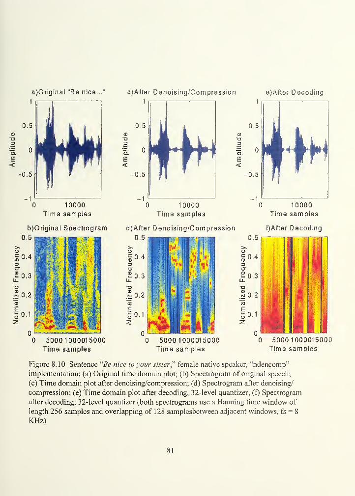
a)Original "Be nice...

CD

3

"q.

E<

-0.5

10000Time samples

b)Original Spectrogram

0.5

50001000015000Time samples

c)After Denoising/Compression

1

e)After Decoding

0.5

CD

X3

ex

E<

-0.5

1

0)

CL

-0.5

10000Time samples

d)After Denoising/Compression

0.5

10000Time samples

f) After Decoding

5000 1000015000Time samples

5000 1000015000Time samples

Figure 8.10 Sentence "Be nice to your sister" female native speaker, "ndencomp"

implementation; (a) Original time domain plot; (b) Spectrogram of original speech;

(c) Time domain plot after denoising/compression; (d) Spectrogram after denoising/

compression; (e) Time domain plot after decoding, 32-level quantizer; (f) Spectrogram

after decoding, 32-level quantizer (both spectrograms use a Harming time window of

length 256 samples and overlapping of 128 samplesbetween adjacent windows, fs = 8

KHz)

81

a)Original "Be nice..."

10000

Time samples

b)Original Spectrogram

0.5

50001000015000Time samples

c)After Denoising/Compression e)After Decoding

1 i 1 1 1

0.5

CD

-aZ3

=5. °

E<

-0.5

-1

J 9 I IF

10000

Time samples

d)After Denoising/Compression

0.5

10000

Time samples

f)After Decoding

5000 1000015000Time samples

50001000015000Time samples

Figure 8.11 Sentence "Be nice to your sister" female native speaker,"ndencomp"

implementation; (a) Original time domain plot;(b) Spectrogram of original speech;

(c) Time domain plot after denoising/compression; (d) Spectrogram after denoising/

compression;(e) After decoding, 64-level quantizer; (f) After decoding, 64-levei

quantizer(both spectrograms use a Harming time window of length 256 samples and

overlapping of 128 samples between adjacent windows, fs = 8 KHz)

82

a)Original "Bye.guys,..." c)After Denoising/Compression e)After Decoding

a4—

*

"5.

E<

-0.5

Time samples^*

b)Original Spectrogram

Time sami

0)

T3

M

E<

Time sam

d)After Denoising/Compression

Time samples.,'

f)After Decoding

u.o

oc 4 I'jjj13

CT

2 0.3u_

Jo.2

E50.1

1 2

Time sami 0" Time sami

Figure 8.12 Sentence "Bye, guys, I'm going back to Brazil," male non-native speaker,

"ndencomp" implementation; (a) Original time domain plot; (b) Spectrogram of original

speech; (c) Plot after denoising/compression; (d) Spectrogram after denoising /

compression; (e) Time domain plot after decoding, 1 6-level quantizer; (f) Spectrogram

after decoding, 1 6-level quantizer (both spectrograms use a Harming time window of

length 256 samples and overlapping of 128 samples between adjacent windows, fs = 8

KHz)

83

a)Original "Bye.guys,..."

1

c)After Denoising/Compression e)After Decoding

CD

-a

*-<

"q.

E<

-0.5

Time sam

b)Original Spectrogram

0.5

o

1 2 3

Time samples _4

0)

T3

"5.

E<

1

0.51 1 1

1

-0.5

CD

-azt>~

Q.

E<

2

Time samples,,*

d)After Denoising/Compression

2

Time samples,,'

f)After Decoding

0.5 0.5

oc 4

20.3LL.

| 0.2

E

'

I .:Time sami

1 2

Time sampmFigure 8.13 Sentence "5ye, gays, /'w gowg back to Brazil" male non-native speaker,

"ndencomp" implementation; (a) Original time domain plot; (b) Spectrogram of original

speech; (c) Plot after denoising/compression; (d) Spectrogram after denoising /

compression; (e) Time domain after decoding, 32-level quantizer; (f) Spectrogram after

decoding, 32-level quantizer (both spectrograms use a Harming time window of length

256 samples and overlapping of 128 samples between adjacent windows, fs = 8 KHz)

84

a)Original "HEY"

0)

-0.5

5000Time samples

b)Original Spectrogram

0.5

200040006000Time samples

c)After Denoising/Compression

1

e)After Decoding

0) 0)

Q.

-0.5 -0.5

5000Time samples

d)After Denoising/Compression

5000Time samples

f)After Decoding

200040006000Time samples

200040006000Time samples

Figure 8.14 Word "Hey," female non-native speaker, "ndencomp" implementation;

(a) Original time domain plot; (b) Spectrogram of original speech; (c) Plot after

denoising/compression; (d) Spectrogram after denoising/compression; (e) Time domain

plot after decoding, 1 6-level quantizer; (f) Spectrogram after decoding, 1 6-level quantizer

(both spectrograms use a Harming time window of length 256 samples and overlapping of

128 samples between adjacent windows, fs = 8KHz)

85

a)Original "HEY"

0)

•an

Q.

E<

c)After Denoising/Compression

1

e)After Decoding

5000

Time samples

b)Original Spectrogram

0.5

cd

a.

5000Time samples

d)After Denoising/Compression

0.5

5000Time samples

f)After Decoding

200040006000Time samples

200040006000Time samples

200040006000Time samples

Figure 8.15 Word "Hey," female non-native speaker, "ndencomp" implementation;

(a) Original time domain plot; (b) Spectrogram of original speech; (c) Plot after

denoising/compression; (d) Spectrogram after denoising/compression;(e) After decoding

32-level quantizer; (f) After decoding, 32-level quantizer (both spectrograms use a

Harming time window of length 256 samples and overlapping of 128 samples

between adjacent windows, fs = 8 KHz)

86

a)Original "HEY"

-a

-0.5

5000

Time samples

b)Original Spectrogram

0.5

200040006000Time samples

c)After Denoising/Compression

1

e)After Decoding

0)

Q.

E<

QJ

-0.5 -0.5

5000Time samples

d)After Denoising/Compression

5000

Time samples

f)After Decoding

U O|

5k 1oc 4 13or

£o.3|u_

a.§0.2l mmE501

1

200040006000Time samples

200040006000Time samples

Figure 8.16 Word "Hey," female non-native speaker, "ndencomp" implementation;

(a) Original time domain plot; (b) Spectrogram of original speech; (c) Plot after

denoising /compression; (d) Spectrogram after denoising/compression;(e) After decoding,

64-level quantizer; (f) After decoding, 64-level quantizer ( both spectrograms use a

Harming time window of length 256 samples and overlapping of 128 samples between

adjacent windows, fs = 8 KHz)

87

a) 'Be nice..." female speaker

1.5

1

i 1

•

0)

T3

"5.

E<

0.5

-0.5

J fl

Hi L

0.5 1 1.5

Time samples .~<

b)ORIGINAL SPECTROGRAM

5000 10000

Time samples15000

c)AFTER DENOISING/COMPRESSION1.5

0.5 1 1.5

Time samples , n'

d)SPECTROGR AM (AFTER)

5000 10000

Time samples

15000

Figure 8.17 Sentence "Be nice to your sister," female native speaker, compressed

with the CPT, "ndencomp" implementation; (a) Original time domain plot;

(b) Spectrogram of original speech; (c) Plot after denoising/compression with 0.85% non-

zero coefficients selected; (d) Spectrogram after denoising/compression ( both

spectrograms use a Harming time window of length 256 samples and overlapping of 128

samples between adjacent windows, fs = 8 KHz)

88

a)Original "Be nice to your sister" c)After Compression w/ "WP"

5000 10000Time Samples

b)Original Spectrogram

15000

5000 10000Time Samples

15000

5000 10000 15000

Time Samples

d)After Compression w/ "WP"

5000 10000

Time Samples15000

Figure 8.18 Sentence "Be nice to your sister,''' female native speaker, compressed

withWPT, using a "Daubechies" basis function; (a) Original time domain plot;

(b) Spectrogram of original speech; (c) Plot after denoising/compression with 15% non-

zero coefficients selected; (d) Spectrogram after compression ( both spectrograms use a

Harming time window of length 256 samples and overlapping of 128 samples between

adjacent windows, fs = 8 KHz)

89

90

IX. CONCLUSION

In this thesis, compression schemes based on the Cosine Packet Transform using

the Local Cosine Transform are presented. The basis functions are chosen via the Best

Basis Algorithm using the entropy minimization criterion.

Coefficients for compression are chosen with an adaptive scheme, which selects

more cosine packet coefficients for voiced intervals than for unvoiced ones. In addition,

since some recorded speech sounds have equipment noise, a denoising scheme is

performed.

Finally, an encoding scheme is implemented. Thus, this study simulates the entire

process of denoising, compression, and encoding (on the transmitter side), as well as

decoding and reconstruction (on the receiver side).

The results obtained are good, due to the combination of certain factors, which

include the following:

(a) Good time and frequency resolution of the local cosine transform;

(b) The Cosine Packet Transform, combined with the Best Basis algorithm using

the entropy minimization criterion allowed not only for minimizing the entropy, but also

for the splitting of the signal into its locally stationary portions. These two factors greatly

contribute to the success of the compression scheme;

(c) The Adaptive Thresholding scheme helps to optimize in quality and quantity

the number of cosine packet coefficients, while preserving good compressed signal

properties;

(d) The denoising scheme allows the number of non-zero coefficients to be

reduced and, at the same time, a better quality of denoised sound when compared to the

original noisy speech.

Through the denoising attempts, it is possible to recognize some patterns of

speech that would be hidden by the higher energy noise in regular compression. The

91

frequency analysis allows differentiating speech sounds and background noise and hence

permits recovering most of the speech sounds.

Basically, two main problems remain. First, there are a few sounds with low

energy that need to be correctly identified and recovered from the background noise. In

the experiments with noisy speech, the only cases that could not be solved are the weak

unvoiced endings, like Ixl at the the word "met," (which is reconstructed like a /d/) and Isi

at the end of words "cats" and "lets", which is lost due to the denoising process. Although

many phonemes were tried, there are probably some others that could have been

attempted and, thus, this is a suggestion for further study. The second problem that was

encountered is quantization noise. Although the encoding scheme works well enough to

make speech recognition for many cases in the simulated receiver sounding "cleaner"

than the original noisy signal, noise is introduced by the quantization process. Although

very small, this noise is enough for cancelling endings like /kt/ in the word "project".

Since this research focused on the compression schemes, less effort is made to develop a

better quantizing and encoding schemes (another point for further study).

The CPT performs better than the WPT for speech compression applications.

When using the WPT, the compression scheme begins losing low energy sounds much

earlier than the CPT, i.e., with a much lower compression ratio, although this may be due

to the basis function that was selected.

The purpose of this study is to find an optimal scheme for the compression of

speech signals. Since the scheme used in this study is successful, speech samples with the

highest possible compression ratios are tested. The quality reconstruction that results for

the majority of tries can be considered as "fair" (see Table 8.1), as shown by the average

mean grades assigned. The very small percentages of selected coefficients in the

compression scheme result tables, and very high compression ratios for the encoding

results, together with a "fair" quality reconstruction indicate a positive overall result. The

compression ratios are not fixed, since the scheme is adaptive to the speech being

analyzed. However our results indicate an average compression ratio of 1:50 on the

92

speech used in our study. The ratio can be adjusted for better quality of reconstructed

sound, according to the needs and availability of the user. Evidently, there will always be

a need to compromise between the compression ratio and the quality of the reconstructed

speech.

93

94

APPENDIX. COMPUTER CODE

% Name: Compcp.m and necompcp.ra

% Subject: Analysis, Compression and Synthesis routine of speech data

% Desccription:

% These two routines contain the following main parts:

% a) Input and loading of speech to be used ( prompts the user for choices like gender of

% speaker, word or sentences among those available and finest depth for time splitting);

% b) Implements the Cosine Packet Transform (CPT) of the speech sequence;

% c) Chooses the basis for the CPT by applying the Best Basis Algorithm;

% d) Implements a Frequency Behavior and an Energy Behavior plot;

% e) Implements a voiced-unvoiced segmentation;

% f) Selects the coefficients by applying the Adaptive Thresholding scheme;

% g) Applies the inverse CPT, by transforming each interval, unfolding and adding it to the

% existing sequence;

% h) Computes and presents the number of non-zero coefficients before and after the

% compression scheme as well as the mean square error between the original and the

% reconstructed sequences;

% i) Presents plots containing the Frequency as well as the Energy behavior; also presents the

% voiced-unvoiced segmentation plot as well as time domain and spectrogram plots of both

% original and reconstructed sequences;

% Notel: Parts b), c) and g) are extracted from the software package Wavelab.600, Stanford

% University[17]. This is also valid for the programs encp6.m, ndencomp.m,

% encptour.m and ndentour.m;

% Note 2: WaveLab code was modified to implement our compression schemes.

% Written and adapted by J. Roberto V. Martins, in October 1995.

% Compcp.m

% Input and loading of speech to be used

clear;

V = input('Please enter "1" for female voice and "2" for a male voice :

');

ifV=lP = 2;

FV = input('Please enter 1 for the sentence, 2 for "be" , 3 for "hate", 4 for "hey" , 5 for "met" , 6 for

"pay", 7 for "cats", 8 for "benice":

');

ifFV=lclear ny;

95

load fse;

ny = [fse*zeros(l,5120)];

elseifFV=2

clear ny;

load fbe;

ny=[fbe'zeros( 1,2048)];

elseifFV=3

clear ny;

load fha;

ny = [fha'zeros(l,7168)];

elseifFV=4

clear ny;

load fhey;

ny = [fhey'];

elseifFV=5

clear ny

load fmet;

ny = [fmet' zeros( 1,1024)];

elseifFV=6

clear ny

load fpay

ny = [fpay' zeros(l,1024)];

elseifFV=7

clear ny

load feats

ny = [ feats1

];

elseifFV=8

clear ny

benice = loadwav('benice.wav');

ny = [(benice(l:16384)/max(abs(benice))+0.01 19)'];

end

end

ifV=2P = 2;

W = input('Please enter l,for "project",2 for "cataratas",3 for "encyclopedia", 4 for "issos",5 for "assos",6

for "six",7 for "the sentence",8 for "aka",9 for "at",10 for "azure",l 1 for "be",12 for "bird",13 for "boot",14

for "call", 15 for "day", 16 for "eka",17 for "epa", 18 for "eve", 19 for "father",20 for "foot", 21 for "for", 22

for "go", 23 for "hate", 24 for "he",25 for "ika",26 for "it",27 for "key",28 for "let",29 for "me",30 for

"met",31 for "no",32 for "obey",33 for "opa",34 for "pay",35 for "read",36 for "see",37 for "she",38 for

"then",39 for "thin" , 40 for "to",41 for "up", 43 for "vote",44 for "we", 45 for "you", 46 for "zoo",47 for

"silence", 48 for "the bye sentence",49 for "beback", 50 for "blows", 51 for "bruna",52 for "adams", 53 for

"sounds good" :

');

ifW=lclear ny;

load newvoice;

ny = y(2700:2700+8191)';

elseifW=2clear ny;

load catar;

ny = ca(1900: 1900+8191)*;

elseifW=3

96

clear ny;

load encic;

ny = en(1200: 1200 +8191)';

elseifW=4clear ny;

load issos

ny = is(1900: 1900+8191)';

elseifW=5clear ny

load assos

ny = as(1900:1900+8191)*;

elseifW=6clear ny

load six

ny = si(l:8192)';

elseifW=7clear ny;

load myvoice;

ny = x(9000:9000+32767)';

elseifW=8clear ny;

load aka;

ny = (ac+0.1656)';

elseifW=9clear ny;

load at;

ny = (at+0.1655)';

elseifW=10clear ny;

load azure;

ny = [(az+0.1651)' zeros(l,6144) ];

elseifW=llclear ny;

load be;

ny = [(be+0.1654)' zeros(l,3072) ];

elseifW=12clear ny;

load bird;

ny = [(bi+0.1658)' zeros(l,7168) ];

elseifW=13

clear ny;

load boot;

ny = [(bo+0.1652)'];

elseifW=14clear ny;

load call;

ny = [(cal+0.1654)' zeros(l,6144) ];

elseifW=15clear ny;

load day;

ny = [(da+0.1645)' zeros(l,1024) ];

elseifW=16clear ny;

load eka;

97

ny = [(ek+0.1653)'];

elseifW=17clear ny;

load epa;

ny = [(ep+0.1650)' zeros(l,6144) ];

elseifW=18clear ny;

load eve;

ny = [(ev+0.1654)' zeros(l,4096) ];

elseifW=19

clear ny;

load father;

ny = [(fa+0.1648)' zeros(l,6144) ];

elseifW=20

clear ny;

load foot;

ny = [(foo+0.1653)' zeros(l,6144) ];

elseifW=21

clear ny;

load for;

ny = [(fo+0.1649)' zeros(l,6144) ];

elseifW=22clear ny;

load go;

ny = [(go+0.1651)'];

elseifW=23clear ny;

load hate;

ny = [(ha+0.1657)' zeros(l,7168) ];

elseifW=24

clear ny;

load he

ny = [(he+0.1657)' zeros( 1,2048) ];

elseifW=25

clear ny;

load ika

ny = [(ik+0.1654)' zeros(l,6144) ];

elseifW=26clear ny;

load it

ny = [(it+0.1657)' zeros( 1,3072) ];

elseifW=27

clear ny;

load key;

ny = [(ke + 0.1652)' zeros( 1,2048)];

elseifW=28

clear ny;

load let;

ny = [(le + 0.1657)'];

elseifW=30clear ny;

load met;

ny = [(met + 0.1 653)*];

elseifW=31

98

clear ny; v

load no;

ny = [(no + 0.1646)' zeros(l,1024)];

elseifW=34

clear ny;

load pay;

ny = [(pa + 0.1655)' zeros(l,1024)];

elseifW=36

load see;

ny = [(se+0.1653)' zeros(l,1024)];

elseifW=37load she;

ny = [(sh+0.1654)'];

elseifW=38

load then;

ny = [(th+0.1656)' zeros(l,6144)];

elseifW=39

load thin;

ny = [(thi + 0.1655)' zeros( 1,1024)];

elseifW=40

load to;

ny = [(to + 0.1649)' zeros(l,3072)];

elseifW=41

load up;

ny = [(up + 0.1653)' zeros( 1,2048)];

elseifW=43load vote;

ny = [(vo + 0.1654)' zeros( 1,1024)];

elseifW=44clear ny;

load weny = [(we+0.1655)' zeros( 1,2048) ];

elseifW=45

clear ny;

load you

ny = [(you + 0.1655)' zeros(l,2048) ];

elseifW=46clear ny;

load zoo

ny = [(zo+0.1646)' zeros( 1,2048) ];

elseifW=47clear ny;

load myvoice;

ny = x(l:8192)';

elseifW=48clear ny;

load bye;

ny = [ bye' zeros(l,9216)];

elseifW=49clear ny;

beback = loadwav('beback.wav');

ny =[ (beback/max(abs(beback))+0.056)' zeros( 1,4824)];

elseifW=50clear ny;

99

blows = loadwav('blows.wav');

ny = [ (blows(l:16384)/max(abs(blows))+0.0034)'];

elseifW=51clear ny;

br = loadwavCbruna.wav');

ny = [ (br/max(abs(br)) + 0.0155)' zeros(l,7268) ];

elseifW=52clear ny;

adam = loadwavCadamsfam.wav');

ny = [ (adam(l:32768)/max(abs(adam)) + 0.0081)'];

elseifW=53clear ny;

load engl6;

ny =[ (engl6(l: 16384) + 3.019e-4)'];

end

end

n = length(ny)

D = input('Enter the finest depth for Time Splitting :

');

% Implementing the Cosine Packet Transform

cp = CPAnalysis(ny,D,'Sine');

stree = CalcStatTree(cp,'Entropy');

[btree,vtree] = BestBasis(stree,D);

[n,L] = size(cp);

% Create Bell

bellname = 'Sine';

m = n / 2AD 12;

[bp,bm] = MakeONBell(bellname,m);

x = zeros(l,n);

% initialize tree traversal stack

stack = zeros(2,2AD+l);

tp = zeros(l,n);

v = zeros(l,n);

compr = zeros( 1 ,n);

coef =zeros(l,n);

ncoef = zeros(l,n);

k=l;stack(:,k) = [0 ]';

v = zeros(l:n);

vs = zeros(l:n);

ind = 0;

le = zeros(l,2AD);

while(k > 0),

d = stack(l,k);b = stack(2,k); k=k-l;

if(btree(node(d,b)) ~= 0) , % nonterminal node

k = k+l;stack(:,k) = [(d+l)(2*b) ]';

100

k = k+1; stack(:,k) = [(d+1) (2*b+l)]';

else

c = cp(packet(d,b,n),d+l)';

coef(l,b/(2Ad).*n+l:(b+l)/(2Ad).*n) = c;

i = (b/(2Ad)*n+l);

len = length(c);

[ I,ND] = max(abs(c));

compr(l,b/(2Ad)*n+l) = length(c);

% Identifying the Frequency Content of each interval

ifND<=round(len/16)

v(i) = 0.25; %itwas0.2

elseifND<= round(len/8)

v(i) = 0.5; % it was 0.4

elseifND < length(c)/(2*P)

v(i)= 1;% it was 0.6

else

[sI,sND] = max(abs([coef(i:i+ND-3),0,0,0,coef(i+ND+l:i+len-l)]));

ifsND>=length(c)/(2*P)

ifND <= lea/2

v(i)= 1.5; %itwas0.75;

elseifND <= len* 3/4

v(i) = 2; % it was 0.9

else

v(i) = 2.5; % it was 1.0

end

elseif sND > round(len/8)

v(i) = 1 ; % it was 0.6

elseif sND > round(len/16)

v(i) = 0.5; % it was 0.4

else

v(i) = 0.25; % it was 0.2

end

end

ec(i:i+len-l) = ones(l,len) .* sum(c.A2); % computing the energy of the coefficients

es(i:i+len-l) = ones(l,len) .* sum(ny(i:i+len-l).A2); % computing the energy of the intervals

vari = std(c);

tp(l,b/(2 Ad).*n+l)=l;

len = length(c);

ind = ind+l;

le(ind) = log2(len);

v(i);

rko = length(c)/16;

ko = ND;

101

fo = 4000/length(c)*ND;

toten = sum(coef.A2);

i = (b/(2Ad)*n+l);

% Applying the Adaptive Thresholding Compression Scheme

if v(i) <= 0.5

if sum(coef(i:compr(i)-l+i).A2) <toten/n * len

iflen<2*n/(2AD)

nncoef(i:compr(i)-l+i) = comp((coef(i:compr(i)-l+i)),99.5);

else

nncoef(i:compr(i)-l+i) = comp((coef(i:compr(i)-l+i)),99.5);

end

else

iflen<2*n/(2AD)

nncoef(i:compr(i)-l+i) = comp((coef(i:compr(i)-l+i)),98.7);

else

nncoef(i:compr(i)-l+i) = comp((coef(i:compr(i)-l+i)),97.66);

end

end

nc= nncoef(i:compr(i)-l+i);

end

if v(i) > 0.5

sumco = sum(coef(i:compr(i)-l+i).A2);

thres = 0.5*toten/n * len;

ifsum(coef(i:compr(i)-l+i).A2)<toten/n * len;

iflen<2*n/(2AD)

nncoef(i:compr(i)-l+i) = comp((coef(i:compr(i)-l+i)),99.5);

else

nncoef(i:len+i-l) = comp(coef(i:len+i-l),99.5);

end

else

iflen<2*n/(2AD)

nncoef(i:compr(i)-l+i) = comp((coef(i:compr(i)-l+i)),99.5);

else

nncoef(i:compr(i)-l+i) = comp(coef(i:compr(i)-l+i),99.5);

end

end

nc = nncoef(i:compr(i)-l+i);

end

ifv(i)> 1

vs(i)=l;

else

if es(i:i+len-l) > (toten/n*2.5*len)

vs(i) = 0.5;

102

end

end

y = dctiv(nc); % Inverse Transforming each interval

% Unfolding each interval and Reconstructing the time sequence after compression

[xc,xl,xr] = unfold(y,bp,bm);

x(packet(d,b,n)) = x(packet(d,b,n)) + xc;

ifb>0,

x(packet(d,b-l,n)) = x(packet(d,b-l,n)) + xl;

else

x(packet(d,0,n)) = x(packet(d,0,n)) + edgeunfold('left',xc,bp,bm);

end

ifb<2Ad-l,x(packet(d,b+l,n)) = x(packet(d,b+l,n)) + xr;

else

x(packet(d,b,n)) = x(packet(d,b,n)) + edgeunfold('right',xc,bp,bm);

end

end

end

nind = sum(le>0);

nle = le(l:nind);

figure(l),plot(ny) , hold;

plot(tp,':'),hold off;

figure(2),plot(ny),hold

plot(v,':'),hold off;

mse = mean((ny - x).A2) % computing the mean square error between the original and

% the reconstructed sequence;

scoefmO = sum(abs(coef)>0) % computing the number of non-zero coefficients before

% compression

sncoefmO = sum(abs(nncoef)>0) % computing the number of non-zero coefficients after

% compression

figure(3),

plot(x);

figure(4),

plot(ec);

figure(5),

plot(es);

figure(6),specgram(ny,[], 1

)

title('Observing the Coarticulation for the sound "ISSOS"')

print figure6-depsc

figure(7),

subplot(3,l,l),plot(ny)

title('Speech Signal: "ISSOS"')

subplot(3,l,2),plot(ny) , hold;

plot(tp,':'),hold off;title('Time Partition')

subplot(3, 1 ,3),plot(ny),hold

plot(v,':'),hold off;title('Frequency Behavior')

figure(8),

subplot(3, 1 , 1 ),plot(ny,'b'),

%plot(v,':'),hold off;

103

title(' "Be nice to your sister'")

subplot(3, 1 ^),plot(vs,*b')

title('Voiced-Unvoiced Segmentation')

subplot(3,l,3),

specgram(ny,[],l)

title('Observing The Spectogram for "Be nice to your sister"')

print figure7 -depsc

% Necompcp.m

% Input and loading of speech to be used

clear;

V = input('Please enter "1" for female voice and "2" for a male voice :

');

ifV=lP = 2;

FV = input(*Please enter 1 for the sentence, 2 for "be" , 3 for "hate", 4 for"hey" , 5 for "met" , 6 for

"pay", 7 for "cats", 8 for "benice" :

');

ifFV=lclear ny;

load fse;

ny = [fse'zeros(l,5120)];

elseifFV=2

clear ny;

load fbe;

ny = [fbe' zeros( 1,2048)];

elseifFV=3

clear ny;

load fha;

ny = [fha'zeros(l,7168)];

elseifFV=4

clear ny;

load fhey;

ny = [fhey'];

elseifFV=5

clear ny

load frnet;

ny = [fmef zeros(l,1024)];

elseifFV=6

clear ny

load fpay

ny = [fpay' zeros(l,1024)];

elseifFV=7

clear ny

load feats

ny = [ feats'];

elseifFV=8

clear ny

benice = loadwav('benice.wav');

ny = [(benice(l:16384)/max(abs(benice))+0.01 19)'];

end

end

ifV=2

104

P = 2;

W = input('Please enter l,for "project",2 for "cataratas",3 for "encyclopedia", 4 for "issos",5 for "assos",6

for "six",7 for "the sentence",8 for "aka",9 for "at", 10 for "azure", 1 1 for "be", 12 for "bird", 13 for "boot", 14

for "call", 15 for "day", 16 for "eka",17 for "epa", 18 for "eve", 19 for "father",20 for "foot", 21 for "for", 22

for "go", 23 for "hate", 24 for "he",25 for "ika",26 for "it",27 for "key",28 for "let",29 for "me",30 for

"met",31 for "no",32 for "obey",33 for "opa",34 for "pay",35 for "read",36 for "see",37 for "she",38 for

"then",39 for "thin" , 40 for "to",41 for "up", 43 for "vote",44 for "we", 45 for "you", 46 for "zoo",47 for

"silence", 48 for "the bye sentence",49 for "beback", 50 for "blows", 51 for "bruna",52 for "adams" :

');

ifW=lclear ny;

load newvoice;

ny = y(2700:2700+8191)';

elseifW=2clear ny;

load catar;

ny = ca(1900: 1900+8 191)';

elseifW=3clear ny;

load encic;

ny = en(1200:1200+8191)';

elseifW=4clear ny;

load issos

ny = is(1900:1900+8191)';

elseifW=5clear ny

load assos

ny = as(1900:1900+8191)';

elseifW=6clear ny

load six

ny = si(l:8192)';

elseifW=7clear ny;

load myvoice;

ny = x(9000:9000+32767)';

elseifW=8clear ny;

load aka;

ny = (ac+0.1656)';

elseifW=9clear ny;

load at;

ny = (at+0.1655)';

elseifW=10clear ny;

load azure;

ny = [(az+0.1651)' zeros(l,6144) ];

elseifW=ll

clear ny;

105

load be;

ny = [(be+0.1654)' zeros(l,3072) ] ;

elseifW= 12

clear ny;

load bird;

ny = [(bi+0.1658)' zeros(l,7168) ];

elseifW= 13

clear ny;

load boot;

ny = [(bo+0.1652)'];

elseifW=14clear ny;

load call;

ny = [(cal+0.1654)' zeros(l,6144) ];

elseifW= 15

clear ny;

load day;

ny = [(da+0.1645)' zeros(l,1024) ];

elseifW= 16

clear ny;

load eka;

ny = [(ek+0.1653)'];

elseifW= 17

clear ny;

load epa;

ny = [(ep+0.1650)' zeros(l,6144) ];

elseifW= 18

clear ny;

load eve;

ny = [(ev+0.1654)' zeros( 1,4096) ];

elseifW=19clear ny;

load father;

ny = [(fa+0.1648)' zeros(l,6144) ];

elseifW=20clear ny;

load foot;

ny = [(foo+0.1653)' zeros(l,6144) ];

elseifW=21clear ny;

load for;

ny = [(fo+0.1649)' zeros(l,6144) ];

elseifW=22clear ny;

load go;

ny = [(go+0.1651)'];

elseif W=23clear ny;

load hate;

ny = [(ha+0.1657)' zeros(l,7168) ];

elseifW=24

clear ny;

106

load he

ny = [(he+0.1657)' zeros(l,2048) ];

elseifW=25clear ny;

load ika

ny = [(ik+0.1654)' zeros(l,6144) ];

elseifW=26clear ny;

load it

ny = [(it+0.1657)' zeros(l,3072) ];

elseifW=27

clear ny;

load key;

ny = [(ke + 0.1652)' zeros( 1,2048)];

elseifW=28clear ny;

load let;

ny=[(le + 0.1657)'];

elseif\V=30

clear ny;

load met;

ny= [(met + 0.1653)'];

elseifW=31

clear ny;

load no;

ny = [(no + 0.1646)' zeros(l,1024)];

elseifW=34clear ny;

load pay;

ny = [(pa + 0.1655)' zeros(l,1024)];

elseifW=36load see;

ny = [(se+0.1653)' zeros(l,1024)];

elseifW=37load she;

ny = [(sh+0.1654)'];

elseifW=38load then;

ny = [(th+0.1656)' zeros(l,6144)];

elseifW=39load thin;

ny = [(thi + 0.1655)' zeros( 1,1024)];

elseifW=40load to;

ny = [(to + 0.1649)' zeros( 1,3072)];

elseifW=41load up;

ny = [(up + 0.1653)' zeros( 1,2048)];

elseifW=43load vote;

ny - [(vo + 0.1654)' zeros(l,1024)];

elseifW=44

107

clear ny;

load weny = [(we+0.1655)' zeros(l,2048) ];

elseifW=45clear ny;

load you

ny = [(you + 0.1655)' zeros( 1,2048) ];

elseifW=46clear ny;

load zoo

ny = [(zo+0.1646)' zeros( 1,2048) ];

elseifW=47clear ny;

load myvoice;

ny = x(l:8192)';

elseifW=48clear ny;

load bye;

ny = [ bye' zeros(l,9216)];

elseifW=49clear ny;

beback = loadwav('beback.wav');

ny = [ (beback/max(abs(beback))+0.056)' zeros( 1,4824)];

elseifW=50clear ny;

blows = loadwav('blows.wav');

ny = [ (blows(l:16384)/max(abs(blows))+0.0034)'];

elseifW=51clear ny;

br = loadwav('bruna.wav');

ny =[ (br/max(abs(br)) + 0.0155)' zeros(l,7268) ];

elseifW=52clear ny;

adam = loadwav('adamsfam.wav');

ny =[(adam(l:32768)/max(abs(adam)) + 0.0081)'];

end

end

n = length(ny)

D = input('Enter the finest depth for Time Splitting :

');

% Implementing the Cosine Packet transform

cp = CPAnalysis(ny,D,'Sine');

stree = CalcStatTree(cp,'Entropy');

[btree,vtree] = BestBasis(stree,D); % Choosing the basis by applying the Best Basis Algorithm

[n,L] = size(cp);

% Create Bell

bellname = 'Sine';

108

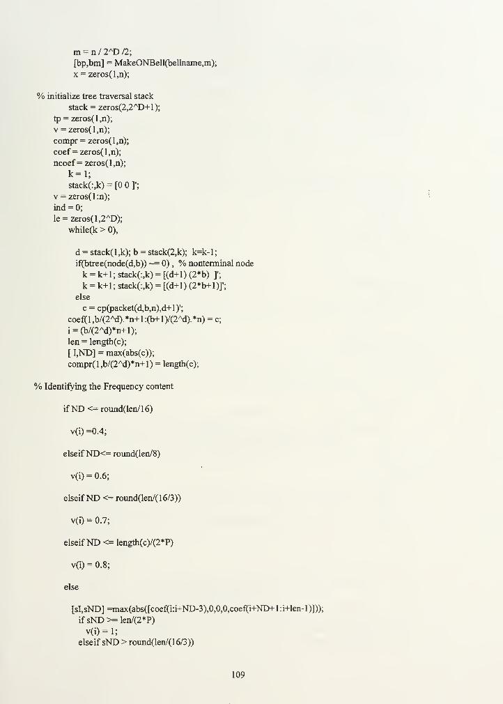
m = n / 2AD 12;

[bp,bm] = MakeONBell(bellname,m);

x = zeros(l,n);

% initialize tree traversal stack

stack = zeros(2,2AD+l);

tp = zeros(l,n);

v = zeros(l,n);

compr = zeros(l,n);

coef=zeros(l,n);

ncoef =zeros(l,n);

k=l;stack(:,k) = [0 ]*;

v = zeros(l:n);

ind = 0;

le = zeros(l,2AD);

while(k > 0),

d = stack(l,k);b = stack(2,k); k=k-l;

if(btree(node(d,b)) ~= 0) , % nonterminal node

k = k+l;stack(:,k) = [(d+l)(2*b) ]';

k = k+1; stack(:,k) = [(d+1) (2*b+l)]';

else

c = cp(packet(d,b,n),d+l)';

coef(l,b/(2Ad).*n+l:(b+l)/(2Ad).*n) = c;

i = (b/(2Ad)*n+l);

len = length(c);

[ I,ND] = max(abs(c));

compr(l,b/(2Ad)*n+l) = length(c);

% Identifying the Frequency content

ifND <= round(len/16)

v(i)=0.4;

elseifND<= round(len/8)

v(i) = 0.6;

elseifND <= round(len/(16/3))

v(i) = 0.7;

elseifND <= length(c)/(2*P)

v(i) = 0.8;

else

[sI,sND] =max(abs([coef(i:i+ND-3),0,0,0,coef(i+ND+l :i+len-l)]));

ifsND>=len/(2*P)

v(i) = l;

elseif sND > round(len/(16/3))

109

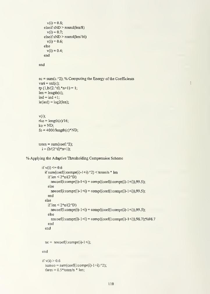
v(i) = 0.8;

elseif sND > round(len/8)

v(i) = 0.7;

elseif sND > round(len/16)

v(i) = 0.6;

else

v(i) = 0.4;

end

end

ec = sum(c.A2); % Computing the Energy of the Coefficients

van = std(c);

tp(l,b/(2.Ad).*n+l)=l;

len = length(c);

ind = ind+1;

le(ind) = log2(len);

v(i);

rko = length(c)/16;

ko = ND;fo = 4000/length(c)*ND;

toten = sum(coef.A2);

i = (b/(2Ad)*n+l);

% Applying the Adaptive Thresholding Compression Scheme

ifv(i)<=0.6

ifsum(coef(i:compr(i)-l+i).A2)<toten/n * len

iflen<2*n/(2AD)

nncoef(i:compr(i)-l+i) = comp((coef(i:compr(i)-l+i)),99.5);

else

nncoef(i:compr(i)-l+i) = comp((coef(i:compr(i)-l+i)),99.5);

end

else

iflen<2*n/(2AD)

nncoef(i:compr(i)-l+i) = comp((coef(i:compr(i)-l+i)),99.5);

else

nncoef(i:compr(i)-l+i) = comp((coef(i:compr(i)-l+i)),98.7);%98.7

end

end

nc = nncoef(i:compr(i)-l+i);

end

ifv(i)>0.6

sumco = sum(coef(i:cornpr(i)-l+i).A2);

thres = 0.5*toten/n * len;

110

if sum(coef(i:compr(i)-l+i).A2) < toten/n * len; % it was 0.5*toten/n*len

iflen<2*n/(2AD)

nncoef(i:compr(i)-l+i) = comp((coef(i:compr(i)-l+i)),99.5);%0.91% for all in "/be nice/"

else

nncoef(i:len+i-l) = comp(coef(i:len+i-l),99.5);

end

else

iflen<2*n/(2AD)

nncoef(i:compr(i)-l+i) = comp((coef(i:compr(i)-l+i)),99.5);

else

nncoef(i:compr(i)-l+i) = comp(coef(i:compr(i)-l+i),99.5);

end

end

nc= nncoef(i:compr(i)-l+i);

end

y = dct_iv(nc); % Inverse transforming each interval

% Unfolding each interval and Reconstructing the time sequence after compression

[xc,xl,xr] = unfold(y,bp,bm);

x(packet(d,b,n)) = x(packet(d,b,n)) + xc;

ifb>0,

x(packet(d,b-l,n)) = x(packet(d,b- 1 ,n)) + xl;

else

x(packet(d,0,n)) = x(packet(d,0,n)) + edgeunfold('left',xc,bp,bm);

end

ifb<2Ad-l,x(packet(d,b+l,n)) = x(packet(d,b+l,n)) + xr;

else

x(packet(d,b,n)) = x(packet(d,b,n)) + edgeunfold('right',xc,bp,bm);

end

end

end

nind = sum(le>0);

nle = le(l:nind);

figure(l),plot(ny) , hold;

plot(tp,':'),hold off;

print figure(l)_deps

figure(2),plot(ny),hold

plot(v,':'),hold off;

print -deps figure2

mse = mean((ny - x).A2) % computing the mean square error between the original and

% the reconstructed sequence;

scoeftnO = sum(abs(coef)>0) % computing the number of non-zero coefficients before

% compression

sncoefmO = sum(abs(nncoef)>0) % computing the number of non-zero coefficients after

% compression

111

figure(3),

plot(x);

fignre(4)

subplot(2,2, 1 ),plot(ny,'b')

title('a)"ISSOS", ORIGINAL PLOP)subplot(2,2,2),plot(x,'b')

title('c)AFTER FIXED THRESHOLDING(0.78%)')

subplot(2,2,3),specgram(ny,[],l)

title('b) SPECTOGRAM')subplot(2,2,4),specgram(x,[],l)

title('d) SPECTOGRAM (AFTER)')

% Name: encp6.m and ndencomp.m

% Subject: Analysis, Denoising/Compression and Synthesis of Speech data;

% Description: These two routines contain the Denoising scheme applied prior to

% the compression schemes;

% The differences between the two routines are in:

% a) The Frequency Identification implementation; for example ndencomp,m

% makes more use of the second largest coefficient than encp6.m does;

% b) The segmentation between voiced and unvoiced segments: encp6.m uses

% 500 Hz for female speech and 1,000 Hz for male speech; ndencomp.m

% uses 1,000Hz for any gender;

%% c) The detection of the presence of low energy speech in high

% energy noisy background, ndencomp.m implements such a scheme, while encp6.m

% doesn't;

%% d) The Adaptive Thresholding Compression Scheme

% Written and adapted by J. Roberto V. Martins, October 1995;

% Encp6.m

clear;

% Input and loading of speech data

V = input('Please enter "1" for female voice and "2" for a male voice :

');

ifV=lP = 8;

FV = input('Please enter 1 for the sentence, 2 for "be" , 3 for "hate", 4 for "hey" , 5 for "met" , 6 for

"pay", 7 for "cats", 8 for "benice" :

');

ifFV= 1

112

clear ny;

load fse;

ny = [fse'zeros(l,5120)];

elseifFV=2clear ny;

load fbe;

ny = [fbe'zeros( 1,2048)];

elseifFV=3

clear ny;

load fha;

ny=[fha*zeros(l,7168)];

elseifFV=4clear ny;

load fhey;

ny = [fhey'];

elseifFV=5clear ny

load finet;

ny = [finef zeros(l,1024)];

elseifFV=6clear ny

load fpay

ny = [fpay1

zeros(l,1024)];

elseifFV=7clear ny

load feats

ny = [ feats1

];

elseifFV=8clear ny

benice = loadwav('benice.wav');

ny = [((benice(l :16384)/max(benice)) + 0.01 19)'];

end

end

ifV=2P = 4;

W = input('Please enter l,for "project",2 for "cataratas",3 for "encyclopedia", 4 for "issos",5 for "assos",6

for "sbc",7 for "the sentence",8 for "aka",9 for "at",10 for "azure",l 1 for "be",12 for "bird",13 for "boot",14

for "call", 15 for "day", 16 for "eka",17 for "epa", 18 for "eve", 19 for "father",20 for "foot", 21 for "for", 22

for "go", 23 for "hate", 24 for "he",25 for "ika",26 for "if',27 for "key",28 for "let",29 for"me",30 for

"met",31 for "no",32 for "obey",33 for "opa",34 for "pay",35 for "read",36 for"see",37 for "she",38 for

"then",39 for "thin" , 40 for "to",41 for "up", 43 for "vote",44 for"we", 45 for "you", 46 for "zoo",47 for

"silence", 48 for "the bye sentence",49 for "beback", 50 for "blows", 5 1 for "bruna", 53 for "sounds good" :

ifW=lclear ny;

load newvoice;

ny = y(2700:2700+8191)';

elseifW=2clear ny;

load catar;

113

ny = ca(1900: 1900+8 191)';

elseifW=3clear ny;

load encic;

ny = en( 1200: 1200 +8191)*;

elseifW=4clear ny;

load issos

ny = is( 1900: 1900+8 191)';

elseifW=5

clear ny

load assos

ny = as(1900: 1900+8191)';

elseifW=6clear ny

load six

ny = si(l:8192)';

elseifW=7clear ny;

load myvoice;

ny = x(9000:9000+32767)';

elseifW=8clear ny;

load aka;

ny = (ac+0.1656)';

elseifW=9clear ny;

load at;

ny = (at+0.1655)';

elseifW=10clear ny;

load azure;

ny = [(az+0.1651)' zeros(l,6144) ];

elseifW=ll

clear ny;

load be;

ny = [(be+0.1654)' zeros( 1,3072) ];

elseifW=12clear ny;

load bird;

ny = [(bi+0.1658)' zeros(l,7168) ];

elseifW=13clear ny;

load boot;

ny = [(bo+0.1652)'];

elseifW=14

clear ny;

load call;

ny = [(cal+0.1654)* zeros(l,6144) ];

elseifW=15clear ny;

load day;

ny = [(da+0.1645)' zeros(l,1024) ];

114

elseifW=16clear ny;

load eka;

ny = [(ek+0.1653)'];

elseifW=17

clear ny;

load epa;

ny = [(ep+0.1650)' zeros(l,6144) ];

elseifW= 18

clear ny;

load eve;

ny = [(ev+0.1654)' zeros( 1,4096) ];

elseifW=19

clear ny;

load father;

ny = [(fa+0.1648)' zeros(l,6144) ];

elseifW=20clear ny;

load foot;

ny - [(foo+0.1653)* zeros(l,6144) ];

elseifW=21clear ny;

load for;

ny = [(fo+0.1649)' zeros(l,6144) ];

elseifW=22clear ny;

load go;

ny = [(go+0.1651)'];

elseifW=23clear ny;

load hate;

ny = [(ha+0.1657)' zeros(l,7168) ];

elseifW=24

clear ny;

load he

ny = [(he+0.1657)' zeros( 1,2048) ];

elseifW=25clear ny;

load ika

ny = [(ik+0.1654)' zeros(l,6144) ];

elseifW=26clear ny;

load it

ny = [(it+0.1657)' zeros( 1,3072) ];

elseif W==27clear ny;

load key;

ny = [(ke + 0.1652)' zeros( 1,2048)];

elseif W==28clear ny;

load let;

ny = [(le + 0.1657)'];

elseifW=30

115

clear ny;

load met;

ny = [(met + 0.1653)'];

elseifW=31clear ny;

load no;

ny = [(no + 0.1646)' zeros(l,1024)];

elseifW=34clear ny;

load pay;

ny = [(pa + 0.1655)' zeros(l,1024)];

elseifW=36load see;

ny = [(se+0.1653)' zeros(l,1024)];

elseifW=37load she;

ny = [(sh+0.1654)'];

elseifW=3 8

load then;

ny = [(th+0.1656)' zeros(l,6144)];

elseifW=39load thin;

ny = [(thi + 0.1655)' zeros(l,1024)];

elseifW=40load to;

ny = [(to + 0.1649)' zeros( 1,3072)];

elseifW=41load up;

ny = [(up + 0.1653)' zeros( 1,2048)];

elseifW=43load vote;

ny = [(vo + 0.1654)* zeros( 1,1024)];

elseifW=44clear ny;

load weny = [(we+0.1655)' zeros( 1,2048) ];

elseifW=45clear ny;

load you

ny - [(you + 0.1655)' zeros( 1,2048) ];

elseifW=46clear ny;

load zoo

ny = [(zo+0.1646)' zeros( 1 ,2048) ];

elseifW =47clear ny;

load myvoice;

ny = x(l:8192)';

elseifW =48clear ny;

load bye;

ny =[ bye' zeros(l,9216)];

elseifW =49clear ny;

116

load beback;

ny =[ (beback- 127.4452)' zeros( 1,4824)];

elseifW=50clear ny;

blows = loadwav ('blows.wav');

ny = [ (blows(l:16384)+0.3027)'];

elseifW=51clear ny;

br = loadwav('bruna.wav');

ny =[ (br/max(abs(br))+0.0155)' zeros( 1,7268)];

elseifW=52clear ny;

br = loadwav('adamsfam.wav');

ny = [ (adam(l:32768)/max(abs(adam))+0.0081)'];

elseifW=53clear ny;

load engl6;

ny = [ (engl6(l: 16384) + 3.019e-4)'];

elseifW=54clear ny;

load voiq;

ny = [voiq(l:32768)'];

end

end

% Implementing the Cosine Packet Transform

n = length(ny)

D = input('Enter the finest depth for Time Splitting :

');

cp = CPAnalysis(ny,D,'Sine');

stree = CalcStatTree(cp,'Entropy');

[btree,vtree] = BestBasis(stree,D);

[n,L] = size(cp);

% Create Bell

bellname = 'Sine';

m = n / 2AD 12;

[bp,bm] = MakeONBell(bellname,m);

%x = zeros(l,n);

%% initialize tree traversal stack

%stack = zeros(2,2AD+l);

tp = zeros(l,n);

v = zeros(l,n);

compr = zeros(l,n);

coef = zeros(l,n);

ncoef=zeros(l,n);

k=l;

117

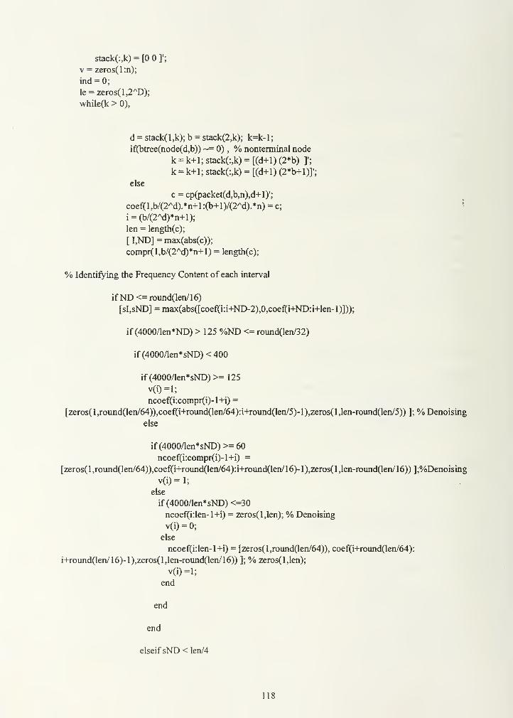
stack(:,k) = [0 ]';

v = zeros(l:n);

ind = 0;

Ie = zeros(l,2AD);

while(k > 0),

d = stack(l,k);b = stack(2,k); k=k-l;

if(btree(node(d,b)) ~= 0) , % nonterminal node

k = k+1; stack(:,k) = [(d+1) (2*b) ]';

k = k+1; stack(:,k) = [(d+1) (2*b+l)]';

else

c = cp(packet(d,b,n),d+l)';

coef(l,b/(2Ad).*n+l:(b+l)/(2Ad).*n) = c;'

i = (b/(2Ad)*n+l);

len = length(c);

[ I,ND] = max(abs(c));

compr(l,b/(2Ad)*n+l) = length(c);

% Identifying the Frequency Content of each interval

ifND<=round(len/16)

[sI,sND] = max(abs([coef(i:i+ND-2),0,coef(i+ND:i+len-l)]));

if (4000/len*ND) > 125 %ND <= round(len/32)

if(4000/len*sND)<400

if(4000/len*sND)>=125

v(i)=l;

ncoef(i:compr(i)-l+i) =

[zeros(l,round(len/64)),coef(i+round(len/64):i+round(len/5)-l),zeros(l,len-round(len/5)) ]; % Denoising

else

if(4000/len*sND)>=60

ncoef(i:compr(i)-l+i) =

[zeros(l,round(len/64)),coef(i+round(len/64):i+round(len/16)-l),zeros(l,len-round(len/16))];%Denoising

v(i)=l;

else

if(4000/len*sND)<=30

ncoef(i:len-l+i) = zeros(l,len); % Denoising

v(i) = 0;

else

ncoef(i:len-l+i) = [zeros(l,round(len/64)), coef(i+round(len/64):

i+round(len/16)-l),zeros(l,len-round(len/16)) ]; % zeros(l,len);

v(i)=l;

end

end

end

elseifsND< len/4

18

ncoef(i:compr(i)- 1 +i) =[zeros( 1 ,len/64),coef(i+round(len/64):i+len- 1 )];%Denoise

v(i)=l;

else

ncoef(i:compr(i)-l+i) =[ zeros(l,len/16),coef(i+len/16:i+len-l) ]; % Denoising

v(i) = 2;

end

end

if (4000/len*ND) <= 125

ifsND<=len/16

ncoef(i:len-l+i) = zeros(l,len); % Denoising

v(i) = 0;

elseifsND <= len/4

if(4000/len*sND)>=300

ncoef(i:i+len-l) = [zeros(l,sND-l),coef(i+sND-l),zeros(l,len-

sND)];%[zeros(l,len/16),coef(i+len/16:i+len-l)];

v(i)=l;

else

ncoef(i:i+len-l) = zeros(l,len); % Denoising

v(i) = 0;

end

else

if(4000/len*ND)<64

ncoef(i:compr(i)-l+i) = zeros(l,len); % Denoising

v(i)=0;

else

ncoef(i:compr(i)-l+i) =[ zeros(l,len/4),coef(i+len/4:i+len-l) ];

v(i) = 2;

end

end

end

elseifND<length(c)/P

[sI,sND] = max(abs([coef(i:i+ND-2),0,coef(i+ND:i+len-l)]));

ifsND<len/32

SND=sNDncoef(i:compr(i) - 1+i) = zeros(l,len); % Denoising

v(i) = 0;

else

v(i)=l;

ncoef(i:compr(i)-l+i) =[ zeros(l,len/16),coef(i+len/16:i+len-l) ]; % Denoising

end

else

[sI,sND] = max(abs([coef(i:i+ND-3),0,0,0,coef(i+ND+l:i+len-l)]));

if sND >= length(c)/(2*P)

v(i) = 2;

ncoef(i:compr(i)-l+i) = [ zeros(l,len/16),coef(i+len/16:i+len-l) ]; % Denoising

else

v(i)=l;

ncoef(i:compr(i)-l+i) = [ zeros(l,len/16),coef(i+len/16:i+len-l) ]; % Denoising

end

end

ec = sum(c.A2);

vari = std(c);

119

tp(l,b/(2.Ad).*n+l)=l;

len = length(c);

ind = ind+1;

le(ind) = log2(len);

v(i);

rko = length(c)/16;

ko = ND;fo = 4000/length(c)*ND;

de(ind) =d;

be(ind) = b;

toten = sum(coef.A2);

i = (b/(2Ad)*n+l);

ifv(i)=nncoef(i:compr(i)-l+i) = ncoef(i:compr(i)-l+i);

nc = nncoef(i:compr(i)-l+i);

end

% Applying the Adaptive Thresholding Compression Scheme

if v(i)= 1

if sum(ncoef(i:compr(i)-l+i).A2) < toten/n * len

iflen<2*n/(2AD)

nncoef(i:compr(i)-l+i) = comp((ncoef(i:compr(i)-l+i)),99.5);

else

nncoef(i:compr(i)-l+i) = comp((ncoef(i:compr(i)-l+i)),99.5);

end

else

iflen<2*n/(2AD)

nncoef(i:compr(i)-l+i) = comp((ncoef(i:compr(i)-l+i)),98.7);

else

nncoef(i:compr(i)-l+i) = comp((ncoef(i:compr(i)-l+i)),97.66);

end

end

nc = nncoef(i:compr(i)-l+i);

end

ifv(i)= 2

sumco = sum(coef(i:compr(i)-l+i).A2);

thres = 0.5*toten/n * len;

if sum(coef(i:compr(i)-l+i).A2) < toten/n * len; % it was 0.5*toten/n*len

iflen<2*n/(2AD)

nncoef(i:compr(i)-l+i) = comp((ncoef(i:compr(i)-l+i)),99.5);

else

nncoef(i:len+i-l) = comp(ncoef(i:len+i-l),99.5);

end

else

iflen<2*n/(2AD)

nncoef(i:compr(i)-l+i) = comp((ncoef(i:compr(i)-l+i)),99.5);

120

else

nncoef(i:compr(i)-l+i) = comp(ncoef(i:corapr(i)-l+i),99.5);

end

end

nc= nncoef(i:compr(i)-l+i);

end

y = dct_iv(nc); % Inverse Transforming each interval

% Unfolding and reconstructing the time sequence after compression

[xc,xl,xr] = unfold(y,bp,bm);

x(packet(d,b,n)) = x(packet(d,b,n)) + xc;

ifb>0,

x(packet(d,b-l,n)) = x(packet(d,b-l,n)) + xl;

else

x(packet(d,0,n)) = x(packet(d,0,n)) + edgeunfold('left',xc,bp,bm);

end

ifb<2Ad-l,x(packet(d,b+l,n)) = x(packet(d,b+l,n)) + xr;

else

x(packet(d,b,n)) = x(packet(d,b,n)) + edgeunfold('right',xc,bp,bm);

end

end

end

nind = sum(le>0);

nle = le(l:nind);

XX = x.*6;

figure(l),plot(ny) , hold;

plot(tp,':'),hold off;

figure(2),plot(ny),hold

plot(v,':'),hold off;

mse = mean((ny - x).A2) % Computing the mean sqare error between the

% original and the reconstructed compressed one

scoefmO = sum(abs(coef)>0)

% Computing the number of non-zero

% coefficients before denoising/compression

sncoefmO = sum(abs(nncoef)>0) % Computing the number of non-zero

% coefficients after denoising/compression

figure(3),

subplot(2,2, 1 ),plot(ny,'b');

title('MET, male speaker');

subplot(2,2,2),plot(x,'b');

title('AFTER DENOISING/COMPRESSION')subplot(2,2,3),specgram(ny);

title('Original Spectogram');

subplot(2,2,4),specgram(x);

title('AFTER DENOISING/COMPRESSION')

121

% Ndencomp.m

% Obs.: This routine has parts a), b) and c) identical to the same parts of

% routine encp6.m. Thus we are only presenting the complement, which begins

% in part d).

compless = 0;

endearly = 0;

% Identifying the Frequency Content of each interval

ifND <= round(len/16); %it was len/64*3

ifND <= round(len/64)

[ sI,sND ]= max(abs([coef(i:i+ND-2),0,coef(i+ND:i+len-l)]));

if (4000/len* sND) <= 300 % try to make it better!!!

iflen>n/(2AD)*8

coef(i+ND-l)=0;

coef(i+sND-l)=0;

[ tI,tND ]= max(abs(coef(i:i+len-l)));% (recovering the "ts" sound)

% implemented to solve problems like in "cats" : it

% still needs to be improved!

!

iftND<round(len/20)

v(i) = 0.1;

else

TND = tND;

compless = 1

;

endearly = 1

;

ncoef(i:i+len-l)=zeros(l,len);%[zeros(l,len/64),coef(i+len/64:i+len-l)];%Denoising

%[zeros( 1 ,tND- 1 ),coef(i+tND- 1 ),zeros( 1 ,len-tND)] ;%[zeros( 1 ,len/64),coef(i+len/64:i+len-

1 )] ;%[zeros( 1 ,tND- 1 ),coef(i+tND- 1 ),zeros( 1 ,len-tND)] ;%[zeros( 1 ,tND- 1 ),coef(i+tND- 1 : i+len- 1 )]

;

end

v(i) = 0.5;

else

v(i) = 0.1;

end

elseif sND <= round(len/8)

ncoef(i:i+len-l) = [ zeros(l,sND-l),coef(i+sND-l),zeros(l,len-sND) ];% Denoising

v(i) = 0.5;

elseif sND <= round(len/4)

ncoef(i: i+len- 1) =[ zeros(l,sND-l),coef(i+sND-l),zeros(l,len-sND) ];% Denoising

v(i)=1.0;

else

v(i) = 0.1;

end

else

122

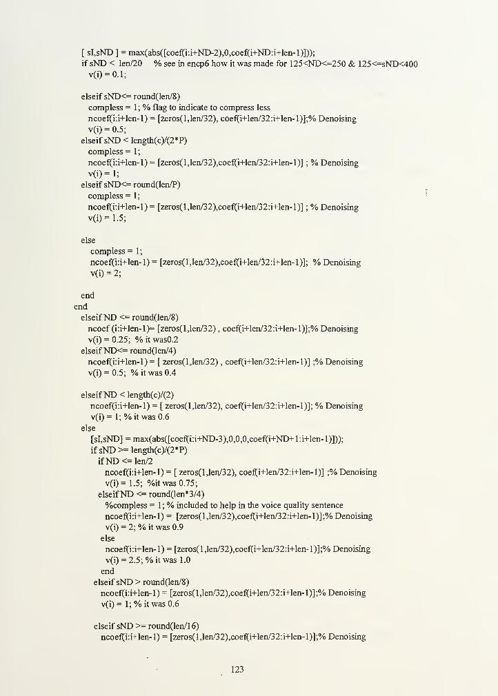
[ sI,sND ] = max(abs([coef(i:i+ND-2),0,coef(i+ND:i+len-l)]));

if sND < len/20 % see in encp6 how it was made for 125<ND<=250 & 125<=sND<400v(i) = 0.1;

elseif sND<= round(Ien/8)

compless = 1 ; % flag to indicate to compress less

ncoef(i:i+len-l) = [zeros(l,len/32), coef(i+len/32:i+len-l)];% Denoising

v(i) = 0.5;

elseif sND < length(c)/(2*P)

compless = 1

;

ncoef(i:i+len-l) = [zeros(l,len/32),coef(i+len/32:i+len-l)] ; % Denoising

v(i) = l;

elseifsND<= round(len/P)

compless = 1

;

ncoef(i:i+len-l) = [zeros(l,len/32),coef(i+len/32:i+len-l)] ; % Denoising

v(i)=1.5;

else

compless = 1

;

ncoef(i:i+len-l) = [zeros(l,len/32),coef(i+len/32:i+len-l)]; % Denoising

v(i) = 2;

end

end

elseifND <= round(len/8)

ncoef (i:i+len-l)= [zeros(l,len/32) , coef(i+len/32:i+len-l)];% Denoising

v(i) = 0.25; %itwas0.2

elseifND<= round(len/4)

ncoef(i:i+len-l) = [ zeros(l,len/32) , coef(i+len/32:i+len-l)] ;% Denoising

v(i) = 0.5; % it was 0.4

elseifND < length(c)/(2)

ncoef(i:i+len-l) = [ zeros(l,len/32), coef(i+len/32:i+len-l)]; % Denoising

v(i)= 1;% it was 0.6

else

[sI,sND] = max(abs([coef(i:i+ND-3),0,0,0,coef(i+ND+l:i+len-l)]));

if sND >= length(c)/(2*P)

ifND <= len/2

ncoef(i:i+len-l) = [ zeros(l,len/32), coef(i+len/32:i+len-l)] ;% Denoising

v(i)=1.5; %it was 0.75;

elseifND <= round(len*3/4)

%compIess = 1 ; % included to help in the voice quality sentence

ncoef(i:i+len-l) = [zeros(l,len/32),coef(i+len/32:i+len-l)];% Denoising

v(i) = 2; % it was 0.9

else

ncoef(i:i+len-l) = [zeros(l,len/32),coef(i+len/32:i+len-l)];% Denoising

v(i) = 2.5;%itwasl.O

end

elseif sND > round(len/8)

ncoef(i:i+len-l) = [zeros(l,len/32),coef(i+len/32:i+len-l)];% Denoising

v(i)= 1;% it was 0.6

elseif sND >= round(len/l 6)

ncoef(i:i+len-l) = [zeros(l,len/32),coef(i+len/32:i+len-l)];% Denoising

123

v(i) - 0.5; % it was 0.4

else

ncoef(i:i+len-l) =[ zeros(l,len/32),coef(i+len/32:i+len-l)];% Denoising

v(i) = 0.25; % it was 0.2

end

end

EC = sum(c.A2);

% Computing the coefficients energy

ec(i:i+len-l) = ones(l,len) * sum(c.A2);

es(i:i+len-l) = ones(l,len) .* sum(ny(i:i+len-l).A2);

% Computing the energy of each interval

vari = std(c);

%ncoef(l,b/(2Ad).*n+l:(b+l)/(2Ad).*n) = nc;

tp(l,b/(2.Ad).*n+l)=l;

len = length(c);

ind = ind+1;

le(ind) = log2(len);

rko = length(c)/16;

ko = ND;fo = 4000/length(c)*ND

de(ind) =d;

be(ind) =b;

toten = sum(coef.A2);

i = (b/(2Ad)*n+l);

% Applying the Adaptive Thresholding Compression Scheme

ifv(i)= 0.1

nncoef(i:i+len-l) = zeros(i:i+len-l);

nc= nncoef(i:compr(i)-l+i);

elseifv(i)<=0.5

if sum(coef(i:compr(i)-l+i).A2) <toten/n * len

iflen<2*n/(2AD)

nncoef(i:compr(i)-l+i) = comp((ncoef(i:compr(i)-l+i)),99.5);

else

nncoef(i:compr(i)-l+i) = comp((ncoef(i:compr(i)-l+i)),99.5);

end

else

iflen<2*n/(2AD)

nncoef(i:compr(i)-l+i) = comp((ncoef(i:compr(i)-l+i)),98.7);

else

nncoef(i:compr(i)-l+i) = comp((ncoef(i:compr(i)-l+i)),97.66);

end

end

nc= nncoef(i:compr(i)-l+i);

end

if v(i) > 0.5 % it was 0.4; % it was= 1

124

sumco = sum(coef(i:compr(i)-l+i).A2);

thres = 0.5*toten/n * len;

if snm(coef(i:compr(i)-l+i).A2) < toten/n * len; % it was 0.5*toten/n*len

iflen<2*n/(2AD)

if compless= 1

nncoef(i:compr(i)-l+i) = comp((ncoef(i:compr(i)-l+i)),97.66);

else

nncoef(i:compr(i)-l+i) = comp((ncoef(i:compr(i)-l+i)),99.5);

end

else

if compless= 1

nncoef(i:compr(i)-l+i) = comp((ncoef(i:compr(i)-l+i)),98.7);

else

nncoef(i:compr(i)-l+i) = comp((ncoef(i:compr(i)-l+i)),99.5);

end

end

else

iflen<2*n/(2AD)

if compless= 1

nncoef(i:compr(i)-l+i) = comp((ncoef(i:compr(i)-l+i)),98.7);

else

nncoef(i:compr(i)-l+i) = comp((ncoef(i:compr(i)-l+i)),99.5);

end

else

%if compless= 1

%nncoef(i:compr(i)-l+i) = comp((ncoef(i:compr(i)-l+i)),98.7);

%else

nncoef(i:compr(i)-l+i) = comp(ncoef(i:compr(i)-l+i),99.5);

%endend

end

nc= nncoef(i:compr(i)-l+i);

end

if endearly= 1

[ma,md] = max(nncoef(i:i+len-l));

end

y = dct_iv(nc);

% Inverse Transforming each interval

if endearly= 1

y = y.*(abs(nncoef(i:i+len-l))>0);

end

% Unfolding and Reconstructing the Time sequence after compression

[xc,xl,xr] = unfold(y,bp,bm);

x(packet(d,b,n)) = x(packet(d,b,n)) + xc;

ifb>0,

x(packet(d,b-l,n)) = x(packet(d,b-l,n)) + xl;

else

x(packet(d,0,n)) = x(packet(d,0,n)) + edgeunfold('left',xc,bp,bm);

end

ifb<2Ad-l,

125

x(packet(d,b+l,n)) = x(packet(d,b+l,n)) + xr;

else

x(packet(d,b,n)) = x(packet(d,b,n)) + edgeunfold('right',xc,bp,bm);

end

end

end

nind = sum(le>0);

nle = le(l:nind);

figure(l),plot(ny) , hold;

plot(tp/:'),hold off;

figure(2),plot(ny),hold

plot(v,':'),hold off;

mse = raean((ny - x).A2)

% Computing the mean sqare error between original signal and the signal after compression

scoefmO = sum(abs(coef)>0)

% Computing the number of non-zero-coefficients before

% denoising/compression

sncoefmO = sum(abs(nncoef)>0)

% Computing the number of non-zero coefficients after

% denoising/compression

figure(3),

plot(x);

figure(4),

plot(ec);

figure(5),

plot(es);

first =1;

nv = zeros(l,length(v));

nnv = zeros(l,length(v));

for i=l:length(v)

ifv(i)>0

ifv(i)<=0.5

nv(i)=1.0;

dist = i - first;

%ifdist>=512

if ec(first) > toten/(n*32)*dist

nnv(first) = nv(first);

nnv(i) = nv(i);

end

first = i;

end

ifv(i)>0.5

nnv(i)= 1.5;

end

end

end

XX = x.*4;

figure(6),plot(ny),hold

plot(nnv,':'),hold off;

figure(7)

subplot(2,2, 1 ),plot(ny,'b')

126

title('"PAY, male speaker'")

subplot(2,2,2),plot(x,'b')

title('AFTER DENOISING/COMPRESSION ')

subplot(2,2,3),specgram(ny,[], 1)

title('ORIGINAL SPECTOGRAM')subplot(2,2,4),specgram(x,[], 1)

title(AFTER DENOISING/COMPRESSION')

% Name: encptour.m and ndentour.m

% Subject: Analysis, Denoising/Compression, Encoding, Decoding and Synthesis

% of speech data

% Description: These two routines were applied on top of encp6.m and

% ndencomp.m. These two programs perform the following tasks in addition to those

% already performed by encp6.m and ndencomp.m:

% a) Implementation of the Linear Quantizer for the Coefficients

% vector;

% b) Encoding of the Locations Vector;

% c) Encoding of the positions of begining of each segment;

% d) Huffman coding of Coefficients Vector and for Locations vector;

% e) Decoding of all the vectors on the Receiver's side

% f) Reconstruction of the Denoised/compressed sequence at the

% receiver's side;

% Obs.: That code is put on top of the existent codes encp6.m and ndencomp.m

% Written by J. Roberto V. Martins, October 1995.

[X,L,seglens,de,be] = enc(nncoef,nle,de,be); % Encoding the locations and coefficients

[TX,prob,nprob,probdesc,N,nq,S] = quantx(X,QL); % Quantizing the coefficients

np = length(probdesc);

avwcoeff= huffcod(np,probdesc); % Huffman coding the coefficients vector

totcoeff = avwcoeff* length(TX);

debe = [debe];

sdebe = size(debe);

ordebe = sort(debe);

ndebe = zeros(l,length(ordebe));

countdb = 1

;

ndebe(l,l) = ordebe(l);

lndb = length(ndebe);

for countdb= 1 :length(debe)-

1

127

if ordebe(countdb+l) > ordebe(countdb)

countdb=countdb+ 1

;

ndebe(countdb) = ordebe(countdb);

end

end

index = 0;

czero = 0;

for countdb =1 :length(ndebe)

if ndebe(countdb) >

index = index +1;

nndebe(index) = ndebe(countdb);

else

czero = czero + 1

;

end

end

probdebe = nndebe/sum(nndebe);

probdbde = fliplr(sort(probdebe));

nprobdbd = probdbde(l:length(probdbde));

avwdebe = huffcod(length(nndebe),nprobdbd); % coding the des and the bes (see chapter VII)

totdebe = avwdebe*(length(debe) - czero) + czero;

[DL,probI,lenprob] = difl(L);

%mDL = max(DL(2:length(DL)));

totndl = 0;

pow = 1

;

forindl=l:length(DL)

while DL(indl) > 2Apow,

pow = pow+1;

end

totndl = totndl + pow; % calculating the necessary number of bits to transmit

NDLwe're not using this

pow =1

;

end

128

totndl = totndl + round(log2(DL(l))) ;% we're using the vector DL to transmit the

locations

sn = 0;

qc = zeros(l,n);

nde = fliplr(de);

nbe = fliplr(be);

nseglens = fliplr(seglens);

nv= 1;

I = nbeJ(2.Ande)*n+l;

forns= l:length(L)

forni= l:length(I)-l

ifL(ns)>=I(ni)

ifL(ns)<=I(ni+l)

sn = sn+1;

SN(sn) = ni;

NDL(sn) = L(ns) - I(ni);

end

end

end

end

pro = SN/sum(SN);

nsimbsn = max(SN) - min(SN) +1;

realpr = zeros(l,nsimbsn);

indsn = 1

;

realpr(indsn) = pro(indsn);

129

for isn = 1 :length(pro)-l

if pro(isn+l)= pro(isn)

realpr(indsn) = realpr(indsn) + pro(isn+l);

else

realpr(indsn+l) = pro(isn+l);

indsn = indsn + 1

;

end

end

desreapr = fliplr(sort(realpr));

RL(1) = DL(1); % Reconstructing L, the locations vector

forcl= l:length(DL)-l

RL(cl+l) = RL(cl) + DL(cl+l);

end

fornv=l:length(nde)-l %i:i+(b/(2Ad)*n-l) l:length(nseglens)

d = nde(nv);

b = nbe(nv);

i = (b/(2Ad)*n+l);

nnc = qcCi^nbeC^nv+^^^deCUnv+l))*^); "/oO^^seglens^+i-l);

thislen = nbe(nv+l)/2Ande(nv+l)*n-i+l

;

for z = i:i + (thislen-1) %(nbe(l,nv+l)/(2Ande(l,nv+l))*n) yol^^seglensOiv)

fort= l:length(RL)

ifz=RL(t)

qc(z) = TX(t)/(nq/2)*S;

end

end

end

130

unfprev = 0;

unfiiex = 0;

nnc = qc(i:(nbe(l,nv+l)/(2Ande(l,nv+l))*n)); ^oCi^^nseglensOO+i-l);

% Inverse transforming to the Time Domain, Unfolding and Reconstructing the Denoised/Compressed

Decoded Speech Sequence

y = dctiv(nnc);

[xc,xl,xr] = unfold(y,bp,bm);

xl(packet(d,b,n)) = xl(packet(d,b,n)) + xc;

ifnv > 1 %nv= 1 %if b>0,

xl(packet(d,b-l,n)) = xl(packet(d,b-l,n)) + xl;

else

xl(packet(d,b,n)) = xl(packet(d,b,n)) + edgeunfold('left',xc,bp,bm);

end

ifb<2Ad-l,

xl(packet(d,b+l,n)) = xl(packet(d,b+l,n)) + xr;

else

xl(packet(d,b,n)) = xl(packet(d,b,n)) + edgeunfold('right',xc,bp,bm);

end

end

figure(5),plot(ny),hold

plot(v,':'),hold off;

mse = mean((x - xl).A2) % Computing the mean square error between the denoised/compressed in

% the trasmitter and the decoded sequence in the receiver;

scoefrnO = sum(abs(coef)>0) % Computing the number of original non-zero coeficients

sncoefinO = sum(abs(nncoef)>0) % Computing the number of non-zero coefficients

% afterdenoising/compression

sqcoefmO = sum(abs(qc)>0) % Computing the number of non-zero coefficients after decoding

figure(6),

plot(x);

figure(7)

subplot(2,3 , 1 ),plot(ny)

title('Original "PAY", Female speaker')

subplot(2,3,2),plot(x)

title('AfterDenoising/Compression')

subplot(2,3,3),plot(xl)

title('After Decoding')

subplot(2,3 ,4),specgram(ny, [] , 1

)

131

title('Original Spectogram')

subplot(2,3,5),specgram(x,[], 1)

title('After Denoising/Compression')

subplot(2,3,6),specgram(xl ,[], 1)

title('After Decoding')

TOTNBITS = totcoeff+ totdebe + totndl

TOTNSAMP = length(TX) + length(debe) + length(SN) + length(NDL)

BITPSAMP = TOTNBITS/TOTNSAMP

COMPRATIO = 100 - (TOTNBITS/(scoefin0*8)*100)

% Name: Comp.m% This function receives as input:

% A vector "c" composed of coefficients and

% a percentage number "pcent";

% As an output, this function gives a vector of same length which the non-zero

% components are the top % dominant (100 - pcent) pcent coefficients extracted from

% that original vector;

% Written by J. Roberto V. Martins in October of 1995.

function cc = comp(c,pcent)

d = sort(abs(c));

p = round(pcent/100*length(c));

for i= l:length(c)

ifp=0cc(i) = c(i);

elseif abs(c(i)) <= d(p)

cc(i) - 0;

else cc(i) = c(i);

end

end

%d = (abs(c)>pcent/100*max(abs(c)));

%cc = c.*d;

% Name: Enc.m

% This function receives a vector, its length and the vectors de

% and be. As an output, it returns:

% X, a vector with non-zero coefficients extracted from the input vector;

% L, the vector containing the locations of the non-zero coefficients from

% the original input vector;

% Written by J. Roberto V. Martins in October of 1995

132

function [X,L,seglens,de,be] = enc(vector,lenvec,de,be)

n = 0;

m=0;

for i = l:length(vector)

if abs(vector(i)) >

n = n+ 1;

X(n) = vector(i);

end

end

for j = 1 : length(vector)

if abs(vector(j))>0

m = m+ 1;

L(m)=j;

end

end

seglens = lenvec;

% Name: Difi.m

% This function encodes a vector by transforming it into a

% differentially encoded vector. It receives the vector to be encoded as an input and returns

% _The differences vector

% _The probabilities vector in descending order as well as its length

function [DL,prob,lendl] = difl(vec)

DL(l) = vec(l);

for z = 2:length(vec)

DL(z) = vec(z) - vec(z-l);

end

a=0;

N = zeros(l,length(DL));

count = 1

;

SDL = sort(DL);

NSDL(l) = SDL(l);

forp= l:length(SDL)-l

ifSDL(p+l)>SDL(p)count = count +1;

NSDL(l,count) = SDL(l,p+l);

end

end

N = zeros(l,length(NSDL));

forl= l:length(DL)

133

forx= l:length(NSDL)

ifDL(l)=NSDL(x)

N(x) = N(x)+l;

end

end

end

end

prob = fliplr(sort(N)/sum(N));

lendl = length(prob);

% Name: Quantx.m

% This function performs the Linear Quantization proposed in this thesis for a

% given input vector. Inputs are the vector X to be quantized and

% the number of quantization levels desired, nq.

% Outputs are:

% _ TX: the quantized vector to be transmitted;

% _ prob: The vector of probabilities of all values in the input vector;

%_ nprob: The new vector of probabilities of all non-zero values in the input vector;

% _ probdesc: The new probabilities vector in descending order for input to Huffman code;

%_ N: The length of probdesc;

%_ nq: The number of quantization levels (equal to the input nq);

% _ S: The scaling factor S, i.e. the highest present absolute value in the vector;

% Written by J.Roberto V. Martins, October 1995.

function [TX,prob,nprob,probdesc,N,nq,S] = quantx(X,nq)

prob = zeros(l,nq+l);

S= max(abs(X));

normX = X/S;

TX = round(normX*nq/2);

%[N,Q] = hist(TX,length(TX));

134

N = zeros(l,nq+l);

STX = sort(TX);

fors= l:length(TX)

forp = -nq/2:l:nq/2

ifTX(s)= pN(l,p+nq/2+l) = N(l,p+nq/2+l) + 1;

end

end

end

prob = N/sum(N);

t = 0;

for s=l :length(prob)

ifprob(s)>0

t = t+l;

nprob(l,t)=prob(l,s);

end

end

probdesc = fliplr(sort(nprob));

Huffcod.m

% This function receives as input

:

% q , the number of symbols; and

% p , the vector containing the probabilities of each symbol;

% As an output, it gives the average word length of the sequence;

% The function uses the code Huffman.m, by K.L. Frack written on 30 November 1993

% Modifications made by J.Roberto V. Martins in October 1995.

% HUFFMAN finds the minimum variance Huffman code for the symbol

% probabilities entered by the user. The algorithm makes use of

% permutation matrices for the combination and sorting of probabilities.

% Permutation matrices are used because they provide a convenient record

% of operations, so that the codewords can then be constructed fairly easily

% once the combination and sorting of probabilities yields just two

% probabilities. At this point a zero is assigned to one of the

% probabilities and a one assigned to the other. The permutation matrices

% are used to append additional zeros and ones as appropriate to obtain

% the final codeword for each symbol.

135

%% Written by K.L. Frack for EC4580 Course Project

% Last Update: 30 November 1993

function [ avwlen ] = huffcod(q,p)

%%/o%%% /o/o%%%%%/o%%%%%%/o%%%%%% /o%/o%%%% /o

% INPUT THE SYMBOLS TO BE CODED %%%%%%%%%%%%% /o%/o%%%%%%%%%%%%%%/o%%%% /o

% INPUT THE NUMBER OF SYMBOLS TO BE CODED. NO TRIVIAL SOLUTION ALLOWED.%q=0; % q = number of symbols. Set to to ensure that the loopo

%while q<3 % Need at least 3 symbols for a non-trivial solution

%q=input('Enter the number of symbols: ');

if q<3,disp(Trivial solution. Use a larger number of symbols.'), end

%end

% ENTER THE SYMBOL PROBABILITIES.

% Note: The probabilities must sum to 1 .00 and must be in entered in

% descending order for the algorithm to work properly. Since the algorithm

% will give erroneous results if these errors are overlooked, error checking

% routines are included in later steps.

%dispC ')

%disp('Enter the symbol probabilities ( in descending order).')

%for i=l:q, p(i)=input([' Enter the probability of s',int2str(i),': ']); end

% ENSURE THERE ARE ENOUGH PROBABILITIES ENTERED% If<RETURN> is inadvertently struck before a probability is entered the

% input command could yield a probability vector which is too small. This

% causes the program to crash. This procedure prevents this from happening

% by setting all of the missing probabilities to zero. In this event the

% user can correct the wrong probabilities in a later step.

if length(p)<q, p=[p;zeros(q-length(p),l)]; end

% ERROR CHECK THE SYMBOL PROBABILITIEScorrect='n'; % correct = 'n' ensures at least once through the error checking

% loop.

count=0; % count = makes the loop a little simpler. It prevents the

% program from prompting for a correction until the loop has

% been executed at least once,

while correct— 'y' % Keep looping until correct.

ifcount>0; % This procedure will be executed only if there are errors

% to be corrected.

s=input('Enter the index of the incorrect probability: ');

p(s)=input(['Enter the correct probability for s',int2str(s),': ']);

end

count=l;

% Display the table.

disp(")

disp('Index Symbol Probability')

disp(' ')

for i=l:q

is=[int2str(i) blanks(6)]; is=is(l:7); % makes a string from the index.

ps=[num2str(p(i)) '000000']; ps=ps(l :6); % makes a string from the prob.

136

disp([' ',is,' s',is,' ',ps]) % displays the table

end

if abs(sum(p)- 1 )> 1 e-8 % Ensures probabilities sum to one.

correct = 'n'; %tinha um "beep," antes

dispC ')

disp('Error —> Probabilities do not sum to 1.00!')

elseif max(diff(p))>0 % Ensures probabilities are in descending order,

correct = 'n';%tinha um "beep" antes

disp(")

disp('Error ~> Probabilities are not in descending order!')

else correct=input('Is the table correct? (Enter y or n): ','s');

% Asks the user to verify that all the probabilities are correctly

% entered. A 'n' response will prompt the user for corrections,

end ?

end, clear correct is ps count

p=p'; % p must be a column vector

pp=p; % pp = extra copy of the original probability vector

%%%%%%%%%%%%%%%%%%%%%%%%%%%%%%%%%%%%%%%%%/o%%%%%%%%%%%%%%%%%%%% FORM THE Q-2 PERMUTATION MATRICES (LEFT MULTIPLICATION) %%%%%%%%%%%%%%%%%%%%%%%%%%%%%%%%%%%%%%%%/o%%%%%%%%%%%%%%%%%%%%%% INITIALIZE EACH MATRIX TO THE ZERO MATRIX OF APPROPRIATE DIMENSIONfor i=l:q-2, eval(['P' int2str(i) -zeros(q-i,q-i+l );']), end

% SUM THE LOWEST TWO PROBABILITIES AND DETERMINE NEW SORTED LOCATIONSfor k=l :q-2 % do for each of the q-2 permutation matrices

Sum=p(q+l-k)+p(q-k); % sum the two lowest (and smallest) probabilities

i=l;

while Sum < p(i) % find highest location in p the vector for the sum

eval(PP int2str(k) "(U) = 1;'])

i=i+l;

end

eval(['P' int2str(k) '(i,q-k:q-k+l) = [1 1];']) % This is the spot

while i<q-k % form rest of matrix with the remaining probabilities

i=i+l;

eval(['P' int2str(k) *(i,i-l) = 1;'])

end

p=eval(['P' int2str(k)])*p; % multiply permutation matrix and probability

% vector to get new probability vector,

end, clear p Sum k

%%%%%%%%%%%%%%%%%%%%%%% FORM THE SYMBOLS %%%%%%%%%%%%%%%%%%%%%%%% The symbols are formed using matrices of characters. The characters are

% ones, zeros, and blanks. Each row in a matrix represents a codeword. The

% final codewords are in the sO matrix. Blanks are included in the matrices

% in order to make this part of the algorithm work efficiently. These blanks

% are removed in a later step.

% INITIALIZE ALL CODEWORD MATRICES TO BLANKS (Blank = 32 in ASCII)

for i=l:q-l, eval(['s' int2str(i-l) - 32*ones(q-i+l,q-i);']), end

% SET RIGHTMOST CODEWORD VECTOR TO ['O' '1']' (0=48 in ASCII, 1=49 in ASCII)

eval(['s' int2str(q-2) '= [48; 49];'])

% WORK FROM RIGHT TO LEFT USING THE P MATRICES TO FORM THE CODEWORDS% The codewords are formed from matrices of zeros (ASCII 48), ones (ASCII 49),

137

% or blanks (ASCII 32). Sq-1 is the rightmost matrix and has the [0 1]'

% matrix. sO is the leftmost matrix and contains the final codewords

% (except for extra blanks).

fori=q-2:-l:l

twosum=find((sum((eval(['P' int2str(i)])'))')=2);

% twosum is the index of the row of the permutation matrix with two ones.

% This is the row which accomplishes the addition of the two lowest

% probabilities. Its index indicates where the sum is to be placed in the

% new probability vector. This index also gives information on how to

% form the codewords.

onesum=find((sum((eval([*P' int2str(i)])'))')= 1 );

% onesum has the indices of all the rows of the permutation matrix with

% only single ones. The indices indicate how the probabilities will be

% placed in the new probability vector. These indices also give

% information on how to form the codewords.

eval(['s' int2str(i-l) '( 1 :q-i- 1 , 1 :q-i- 1 )=s' int2str(i) '(onesum, liq-i-1);1

])

eval(['s' int2str(i-l) '(q-i ,l:q-i-l)=s' int2str(i) '(twosum, l:q-i-l);'])

eval(['s' int2str(i-l) '(q-i+l,l:q-i-l)=s' int2str(i) '(twosum, l:q-i-l);'])

eval(['s' int2str(i-l) '(q-i ,q-i)=48;'])

eval(['s' int2str(i-l) '(q-i+l,q-i)=49;'])

% The five lines above place the appropriate ones, zeros, and blanks in the

% codeword matrices as the progression moves from the right to the left.

eval(['clear P int2str(i) ' s' int2str(i)])

end, clear onesum twosum

% FIND AND REMOVE THE BLANKS FROM EACH CODEWORD AND COMPUTE WORDLENGTHSfor i=l:q

eval(['S' int2str(i) '= (s0(i, :));*]) % sO has all the needed information

eval(['c=find(S' int2str(i) '= 32);']) % find all the blanks

eval(['S' int2str(i) '(c) = [];']) % remove all the blanks

eval(['S' int2str(i) '= setstr(S' int2str(i) ');']) % convert from ASCII

eval(['L(i)=length(S' int2str(i) ');']) % compute the length of each codeword

end, clear sO c

avwlen = sum(L*pp);

%%%%%%%%%%%%%%%%%%%%%%%%% DISPLAY THE OUTPUT %%%%%%%%%%%%%%%%%%%%%%%%%disp(")

dispCSymbol Probability Code Word')

disp(' ')

for i=l:q

is=[int2str(i) blanks(6)]; is=is(l:7);

ps=[num2str(pp(i)) '000000']; ps=ps(l:6);

disp([' s'.is,' ',ps,' ',eval(['S' int2str(i)])])

end, clear is ps i q, disp(' ')

% COMPUTE AND DISPLAY AVERAGE WORD LENGTHL_avg=sum(L *

pp);

disp(['The average word length is ', num2str(L_avg)])

% COMPUTE AND DISPLAY THE ENTROPYH=sum(pp. * log2( 1 ./pp));

disp(['The entropy is ', num2str(H)])

% COMPUTE AND DISPLAY VARIANCEvar=sum(((L_avg-L).A2)*pp);

disp(['The variance is ', num2str(var)])

138

LIST OF REFERENCES

1. Deller, J., Proakis, J.G., and Hansen, J. H., Discrete Time Processing Signals. Mac-

Millan Publishing Co., Englewood Cliffs, NJ, 1993.

2. Wickerhauser, M.V., Adapted Wavelet Analysis From Theory to Software. A.K.

Peters, Ltd., Wellesley, MA, 1994.

3. Malvar, H.S. and Staelin, D.H., "Reduction of Blocking Effects in Image Coding with

a Lapped Orthogonal Transform," Proceedings ofthe ICASSP '88, New York, April,

1988, pp. 781-784.

4. Coifman, R. and Meyer, Y., "Remarques sur l'analyse de Fourier a fenetre," C.R.

Acad. Sci., Paris Ser. 7(1991), pp. 259-261.

5. Meyer, Y., Wavelets: Algorithms and Applications, Siam, Philadelphia, PA, 1993.

6. Malvar, H.S. , "Transform/Subband Coding of Speech with the Lapped Orthogonal

Transform," Proceedings of the ISCAS '89, Portland, OR, May, 1989, pp. 1268-1271.

7. Mallat, S.G., "A Theory for Multiresolution in Signal Decomposition: The Wavelet

Representation," IEEE Transactions on Pattern Analysis and Machine Intelligence,

vol. 11, pp. 674-693, July, 1989.

8. Cody, M.A., "Wavelet Packet Transform," Dr. Dobb's Journal, April, 1994.

9. Rioul, O. and Vetterli, M., "Wavelets and Signal Processing," IEEE Signal Pro-

cessing, pp. 14-18, October, 1991.

10. Daubechies, I., "Ten Lectures on Wavelets," SIAM, Philadelphia, PA, 1992.

11. Malvar, H.S., "Lapped Transforms for Efficient Transform/Subband Coding," IEEE

Transactions onASSP, vol. 38, no. 6, June, 1990.

12. Rabbani, M. and Jones, P.W., "Digital Image Compression Techniques," SPIE, Bel-

lingham,WA, 1991.

13. Wesfreid, E. and Wickerhauser, M.V., "Adapted Local Trigonometric Transforms

and Speech Signal Processing," IEEE Transactions on Signal Processing, Vol. 41,

No.12, pp. 3596-3600, Dec. 1993.

14. Weiss, J. and Schremp, D., "Putting Data on a Diet," IEEE Spectrum, pp. 36-39,

August, 1993.

139

15. Jayant, N.S. and Noll, P., Digital Coding of Waveforms, Prentice Hall, Englewood

Cliffs, NJ, 1984.

16. Brown, D.W., SPCToolbox, MSEE Thesis, Naval Postgraduate School, Monterey,

CA, 1995.

17. Buckheit J., Chen S., Donoho D.L., Johnstone I.M. and Scargle J., Wavelab 0.600,

Stanford University, Stanford, CA, 1994.

140

INITIAL DISTRIBUTION LIST

1. Defense Technical Information Center 2

8275 John J. Kingman Rd., STE 0944

Ft. Belvoir, VA 22060-6218

2. Dudley Knox Library 2

Naval Postgraduate School

411 DyerRd.

Monterey, CA 93943-5101

3. Chairman, Code EC 1

Department of Electrical and Computer Engineering

Naval Postgraduate School

Monterey, CA 93943-5121

4. Professor Monique P. Fargues, Code EC/Fa 2

Department of Electrical and Computer Engineering

Naval Postgraduate School

Monterey, CA 93943-5121

5. Professor Ralph Hippenstiel, Code EC/Hi 1

Department of Electrical and Computer Engineering

Naval Postgraduate School

Monterey, CA 93943-5121

6. Prof. Murali Tummala, Code EC/Tu 1

Department of Electrical and Computer Engineering

Naval Postgraduate School

Monterey, CA 93943-5121

7. Estado Maior da Armada 1

A/C Brazilian Naval Commission

4706 Wisconsin Ave., N.W.

Washington, DC 20016

8. Instituto de Pesquisas da Marinha 1

Diretor

A/C Brazilian Naval Commission

4706 Wisconsin Ave., N.W.

Washington, DC 20016

141

Grupo de Sistemas Digitals

Rua Ipiru 2, Ilha do Governador,

Rio de Janeiro, BRAZIL 21931

10. Diretoria de Sistemas de Armas da Marinha

A/C Brazilian Naval Commission

4706 Wisconsin Ave., N.W.

Washington, DC 20016

11. Diretoria de Ensino da Marinha

A/C Brazilian Naval Commission

4706 Wisconsin Ave., N.W.

Washington, DC 20016

12. Centro de Analises de Sistemas Navais

.

A/C Brazilian Naval Commission

4706 Wisconsin Ave., N.W.

Washington, DC 20016

13. Diretoria de Telecomunicacoes da Marinha

A/C Brazilian Naval Commission

4706 Wisconsin Ave., N.W.

Washington, DC 20016

14. Coordenadoria de Projetos Especiais (COPESP)

A/C Brazilian Naval Commission

4706 Wisconsin Ave., N.W.

Washington, DC 20016

15. LCDR. Joao Roberto V. Martins .

Instituto de Pesquisas da Marinha

A/C Brazilian Naval Commission

4706 Wisconsin Ave., N.W.

Washington, DC 20016

142

DUDLEY KNOX LIBRARY

NAVAL POSTGRADUATE SCHOOL

MONTEREY CA 93943-5101

UUULC1 r\INWA LIDMAMT

3 2768 00323026 9