Event Model Decomposition(version 1.3 April 2009)

J.R. Abrial ETHZ

1 Introduction

Developing an event model by successive refinements usually starts with very few events (sometimeseven a single event) and with a very few state variables. On the contrary, it usually ends up with a lastrefinement step dealing with many events and many variables. This is because one of the most importantmechanism of the Event-B approach consists in introducing new events during refinement steps. The re-finement mechanism is also used at the same time to significantly enlarge the number of state variables.

At some point, we might have so many events and so many state variables that the refinement pro-cess might become quite heavy. And we may also figure out that the refinement steps we are trying toundertake are not involving any more the totality of our system (as was the case at the beginning of thedevelopment), only a few variables and events are concerned, the others playing a passive role only.

The idea of model decomposition is thus clearly very attractive: it consists in cutting an heavy eventsystem into smaller pieces which can be handled more comfortably than the whole. More precisely, eachpiece should be able to be refined independently of the others. But, of course, the constraint that must besatisfied by this decomposition is that such independently refined pieces could always (in principle) beeasily re-composed. This re-composition process should then result in a system which could have beenobtained directly without the decomposition, which thus appears to be just a kind of “divide-and-conquer”artefact.

But this is clearly not the only interesting methodological outcome of decomposition. It also allows usto build up the architecture of our future system by dividing it into independent components with welldefined relationship. This last important point will be fully explained in what follows.

This paper contains the feasibility study of such a mechanism. After proposing an informal definition ofdecomposition in the next section, we outline the methodological outcome and constraints of this approach(sections 3). We then present its main difficulty (section 4) and propose a solution to it (section 5), whichnevertheless presents a certain limitation (as explained in section 5.1). In section 6, a short example showsthe mechanism at work. In section 7, we present another example explaining how the main limitationof this approach, as described in section 5.1, can be overcome. The proof that guarantees a well-definedmathematical approach to decomposition is developed in the Appendix.

2 Informal Definition

Decomposing an event modelM is defined as follows:

1. M is split into several sub-models, say N , . . . , P .

2. The events ofM are partitioned and the elements of this partition form the events of the sub-models.

3. We shall see in section 4 how the variables of modelM are also distributed among the sub-models.

4. These sub-models are then refined several times independently yielding eventually NR, . . . , PR.

1

5. These refined models might be put together to form a re-composed modelMR.

6. The re-composed modelMR must be guaranteed to be a refinement ofM.

This process is illustrated in the following diagram:

r

Decomposition Refinement Recomposition

M →

N → NR

· · ·

P → PR

→ MR

It is important to notice here that point 5 above (the recomposition) will never be performed in practice.One has only to figure out that it can be done and that the refinement condition stated in point 6 (MR isa refinement ofM) must then be satisfied.

3 Methodological Outcome and Constraints of Decomposition

This decomposition process may play five important practical methodological roles:

1. It is certainly easier to refine sub-models N , . . . , P independently rather than together.

2. Refinements of sub-models N , . . . , P can be further decomposed in the same way, and so on.

3. Sub-models N , . . . , P could already possess some refinements able to be reused in several projects.

4. Decomposition is the basis for building the architecture of the final system we want to build.

5. A consequence of decomposition is that several independent users can work on the sub-models

Point 3 above is methodologically very important. It shows how decomposition and composition are tiedtogether. In other words, we decompose in order to be able to compose several existing models taken offthe shelf. By having a decomposition phase done before the composition one, we ensure that the compo-sition leads to a correct global model, namely the one presented before the decomposition.

Our decomposition approach shall obey two main constraints:

1. We must define a process that is totally robust mathematically speaking.

2. We do not want to modify in any way the mathematical definition and concept of refinement.

4 The Main Difficulty: Variable Distribution

The difficulty with the variable distribution is better illustrated with a simple example.

Suppose that we have a certain model, M, with four events e1, e2, e3 et e4. We would like to de-compose M into two separate models: (1) N dealing with events e1 and e2, and (2) P dealing with

2

events e3 and e4. We are interested in doing this decomposition because we know that there are somenice refinements that can be performed on e1 and e2 and, independently, on e3 and e4.

But in doing this event partition we must also perform a certain variable distribution. Suppose that wehave three variables v1, v2 and v3 inM. Like the events, the variables must be split too. For instance, wemight put v1 and v2 with N (because e1 and e2 are supposedly working with them and not with v3). Asa result, v3 goes, quite naturally, with P . But the difficulty here is that e3 and e4, which work with v3,might also work with v2. So, besides v3, P certainly also requires v2 to deal correctly with e3 and e4. Insummary: (1) e1 and e2 work with v1 and v2, and (2) e3 and e4 work with v2 and v3. So N must havevariables v1 and v2 and P must have variables v2 and v3. Variable v2 is common to both N and P .

The problem seems unsolvable since, apparently, there will always be some variables that are neededin several decomposed models. In other words, the splitting of the events will always conflict with thatof the variables. Notice however that this should not be surprising: after all, variable v2 is simply thecommunication channel situated between sub-models N and P .

So, the question of common variables, v2 in our example, is unavoidable. How are we going to solvethis difficulty?

5 The Solution: Shared Variables and External Events

5.1 Shared Variables

We have no choice: the shared common variables must clearly be replicated in the various components ofour decomposition. Notice that the shared variables in question can be modified by any of the components:we do not want to make any specialization of the components, some of them being only allowed to read,while some other to write these variables. We know that it is not possible in general.

The new difficulty that arises immediately at this point concerns the problem of refinement. In princi-ple, each component can freely data-refine its state space. So that the same replicated variable could, inprinciple, be refined in one way in one component and differently in another: this is not acceptable sincethen the two components cannot communicate as they are not using the same conventions on the sharedvariable.

The price to pay in order to solve this difficulty is to give the replicated variables a special status in thecomponents where they stay. A shared variable has a simple limitation: it must always be present in thestate space of any refinement of the component. In other words, a shared variable cannot be data-refined.We shall see in section 7 how this limitation can be partially overcome.

Notice that there is no theoretical impossibilities to have the shared variables being refined. But thenagain the same shared variable has to be refined in the same way in each independent sub-model. This isnot very convenient as we want the sub-models to be genuinely independent.

5.2 External Events

The notion of shared replicated variables we introduced in the previous section is not sufficient. Supposethat in a certain component a shared variable is only read, not written. The trouble with that shared vari-able is that it has suddenly become a constant in that component, which is certainly not what we want.

What we need thus in each component, is a number of additional events simulating the way our sharedvariables are handled in the non-decomposed model. Such events are called external events. Each of themmimics, using the shared variables only, an event of the non-decomposed model that modifies the sharedvariables in question. The reader has understood: mimic simply means “is an abstraction of”. Of coursesuch external events cannot be refined in their component. In section 5.4 we explain how the external

3

events are practically constructed.

Notice that there is a distinction to be made between a shared variable and an external event. A sharedvariable is shared in all sub-models where it can be found, whereas an external event always has a non-external counterpart elsewhere. An event, however, can be external in several sub-models.

Notice finally that the external events are just modeling artefacts. In fact, the final code produced out ofthe last refinements of the sub-models does not contain any translation attached to the external events.

5.3 About the InvariantsIn previous sections, we explained how the events and the variables are distributed among the sub-models.But we did not mentioned the invariants. Their destination is simple:

1. An Invariant dealing with the private variables of a sub-model is copied in that sub-model.

2. An invariant involving a shared variable only is copied in the sub-models where this variable is shared.

3. An invariant involving a shared variable together with other variables is not copied.

5.4 Final RecompositionThe re-composition of refinements of the various sub-models is now extremely simple. We put togetherall the variables of the individual sub-models (with the various shared variables incorporated only once)and we simply throw away all the external events of each sub-model.

It remains now for us to prove that the re-composed model is indeed a refinement of the initial one.Notice again that this re-composition will never be done: it is simply a thought experiment. In otherwords, it is just something that could be done, and which must then yield a refinement of the initialnon-decomposed model. The proof that the re-composition is indeed a refinement of the original non-decomposed model is shown in the Appendix.

5.5 Practical Construction of External EventsAn external event is the projection of the original event on the state of the sub-model. Practically, this canbe done in a very systematic manner by replacing the disappearing variables by simple parameters of theexternal events. This can be illustrated on a simple example. Let e2 be an event of the original model.Suppose that the original model deals with variables v1, v2, and v3. Suppose that the event e2 does notwork with variable v3. Here is thus the event e2:

e2when

G(v1, v2)then

v1 := E(v1, v2)v2 := F (v1, v2)

end

The projection of e2 on a state made of variable v3 together with shared variable v2 is as follows:

external_e2any x1 where

G(x1, v2)then

v2 := F (x1, v2)end

4

As can be seen, the variable v1 occurring in e2 has been replaced by the parameter x1 and the assignmentto v1 in e2 has disappeared. It might sometimes be necessary to add an additional guard in order to definethe type of parameter x1. In the more general case where the action in non-deterministic as in:

e2when

G(v1, v2)then

v1, v2 :| P (v1, v2, v1′, v2′)end

then the projection of e2 on a state made of variable v3 together with shared variable v2 is as follows:

external_e2any x1 where

G(x1, v2)then

v2 :| ∃y1 · P (x1, v2, y1, v2′)end

5.6 Tool Requirements for Decomposition

The requirements for a tool able to help users decomposing a model are rather simple:

1. Given a model to be decomposed, the user must be able to designate the various elements of thedecomposed sub-models: what are their private events, what are their external events, what are theirprivate variables, what are the shared variables.

2. The tool must verify that all events and all variables are indeed well partitioned and distributed.

3. The tool must then generate the external events (as shown in the previous section) to be incorporatedin each decomposed sub-model.

4. Finally, the tool must generate the various independent decomposed sub-model.

Notice that some extensions to the basic Rodin Platform tools have to be undertaken. We have tointroduce the notion of shared variables in a model as well as that of external events. Let us recall thatshared variables and external events must not be refined.

6 A Short Example

In this section,we propose a short example. It is a rather toyish and very artificial example however. Itsrole is simply to illustrate what we have described so far.

6.1 The Initial Model

In an initial modelM, we have three variables a, b, and c handling some natural number values. Thesevariables are “controlled” by three boolean variables m, n, and p respectively. We also have four eventsnamed in_a, a_2_b, b_2_c, and out_c. These events respectively insert a new value in a (in_a), movevalues from a to b (a_2_b), and from b to c (b_2_c), and finally remove values from c (out_c). This isshown in the following diagram:

5

in_a a_2_b b_2_c out_c−→ a −→ b −→ c −→

The moving of the values should respect some constraints handled by the boolean control variables m,n, and p. When the control variable m is equal to TRUE, this means that the value of a is fresh so that itcan be sent to b. This, however, can only be performed provided the value of b is old, meaning that it hasalready been sent to c: this fact is recorded by the value of n, the boolean variable controlling b, when itis equal to FALSE. Boolean variable p play a similar role with c. Next are the typing of the variables andthe definition of the various events:

variables: ambncp

inv0_1: a ∈ Ninv0_2: m ∈ BOOLinv0_3: b ∈ Ninv0_4: n ∈ BOOLinv0_5: c ∈ Ninv0_6: p ∈ BOOL

INITa := 0m := FALSEb := 0n := FALSEc := 0p := FALSE

in_awhen

m = FALSEthen

a :∈ Nm := TRUE

end

a_2_bwhen

m = TRUEn = FALSE

thenb := am := FALSEn := TRUE

end

b_2_cwhen

n = TRUEp = FALSE

thenc := bn := FALSEp := TRUE

end

out_cwhen

p = TRUEthen

p := FALSEend

6.2 Preparing the Decomposition

Our purpose is now to decompose the model M presented in previous section into two separate sub-modelsN andP as shown in the following figure. Sub-modelN contains events in_a and a_2_b togetherwith variables a and m, whereas sub-model P contains events b_2_c and out_c together with variablesc and p:

ma

pc

b_2_c

out_c

in_a

a_2_b

N P

b

n

Variables b and n are the shared variables forming the channels between the two sub-models. We cansee that sub-model N modifies the shared variable b (write) while sub-model P only access it (read).However, both sub-models modify and access the shared variable n. In other words, the "channel" n isfull-duplex.

It might be interesting to simplify this and replace the full-duplex channel n by two simple channels. So,before doing our decomposition we might first refine our modelM to modelM1. We replace the variablen by two bit variables r and s. The variable r is modified by the event a_2_b, whereas the variable s isaccessed only by this event. We have a symmetric situation with event b_2_c. Here are the variables andevents of refinementM1:

6

variables: ambcprs

inv1_1: r ∈ {0, 1}inv1_2: s ∈ {0, 1}inv1_3: r = s ⇔ n = FALSE

INITa := 0m := FALSEb := 0c := 0p := FALSEr := 0s := 0

Invariant inv1_3 shows how concrete variables r and s are glued to the abstract variable n. Notice thatthis invariant could have been written equivalently as n = bool(r 6= s).

in_awhen

m = FALSEthen

a :∈ Nm := TRUE

end

a_2_bwhen

m = TRUEr = s

thenb := am := FALSEr := 1− r

end

b_2_cwhen

r 6= sp = FALSE

thenc := bs := 1− sp := TRUE

end

out_cwhen

p = TRUEthen

p := FALSEend

What is shown here with variables r and s is the classical alternating bit protocol.

6.3 The Decomposition

We now propose the following decomposition with simple channels only:

ma

pc

b_2_c

out_c

in_a

a_2_b

N P

b

r

s

The model N has proper events in_a and a_2_b, which are thus exact copies of events bearing thesame names in model M1. Moreover, the external event external_b_2_c, is then a projection of theevent bearing the name b_2_c in the initial modelM1. ModelN has five variables a, m, b, r, and s. Thelast three are shared as indicated below.

variables: am

shared: brs

inv_N0_1: a ∈ Ninv_N0_2: m ∈ BOOLinv_N0_3: b ∈ Ninv_N0_4: r ∈ {0, 1}inv_N0_5: s ∈ {0, 1}

INITa := 0m := FALSEb := 0r := 0s := 0

Notice that in the INIT event, the initialization of the variable s is rather an external initialization.

7

in_awhen

m = FALSEthen

a :∈ Nm := TRUE

end

a_2_bwhen

m = TRUEr = s

thenb := am := FALSEr := 1− r

end

external_b_2_cwhen

r 6= sthen

s := 1− send

Notice that the event external_b_2_c should be the following according to what has been said in section5.4, but this is clearly equivalent to what we wrote above because the parameter xp has no influence onthe action and the guard ∃xp · xp = FALSE holds trivially:

external_b_2_cany xp where

xp = FALSEr 6= s

thens := 1− s

end

Next is our second decomposed model P . It is organized symmetrically to N . Likewise, the externalevent external_a_2_b is a projection of the event a_2_b inM1.

variables: cp

shared: brs

inv_P0_1: c ∈ Ninv_P0_2: p ∈ BOOLinv_P0_3: b ∈ Ninv_P0_4: r ∈ {0, 1}inv_P0_4: s ∈ {0, 1}

INITc := 0p := FALSEb := 0r := 0s := 0

Similarly to what we observed above for modelN , here in the INIT event the initialization of the variabler is rather an external initialization.

external_a_2_bany x where

x ∈ Nr = s

thenb := xr := 1− r

end

b_2_cwhen

r 6= sp = FALSE

thenc := bs := 1− sp := TRUE

end

out_cwhen

p = TRUEthen

p := FALSEend

6.4 Refinements

We now refineN toNR. The refinement consists of adding a new variable d. The value of the variable ais gradually moved to d by incrementing d. For this, we introduce a new convergent event named inc_d.Next are the events of NR. Notice that the event external_b_2_c is not modified).

8

in_awhen

m = FALSEthen

a :∈ Nm := TRUE

end

inc_dstatus

convergentwhen

m = TRUEd 6= a

thend := d + 1

end

a_2_bwhen

m = TRUEr = sd = a

thenb := dm := FALSEr := 1− rd := 0

end

external_b_2_cwhen

r 6= sthen

s := 1− send

In order to prove the convergence of the event inc_d, we have to exhibit a variant, which is clearly thefollowing:

variant_NR: a− d

Now proving that this variant is a natural number requires that d is always less than or equal to a. In turn,proving this invariant requires an additional invariant as shown below:

inv_NR_1: d ≤ a

inv_NR_2: m = FALSE ⇒ d = 0

We now refine similarly P to PR. The refinement consists of adding a new variable e. The value ofthe variable b is gradually moved to e by incrementing e. For this, we introduce a new convergent eventinc_e. Next are the events of PR. Notice that the event external_a_2_b is not modified.

external_a_2_bany x where

x ∈ Nr = s

thenb := xr := 1− r

end

inc_estatus

convergentwhen

n = TRUEe 6= b

thene := e + 1

end

b_2_cwhen

r 6= sp = FALSEe = b

thenc := es := 1− sp := TRUEe := 0

end

out_cwhen

p = TRUEthen

p := FALSEend

Similar considerations as done for the previous refinement lead to the following variant and invariants:

variant_PR: b− einv_PR_1: e ≤ b

inv_PR_2: n = FALSE ⇒ e = 0

9

6.5 Summary of the Development

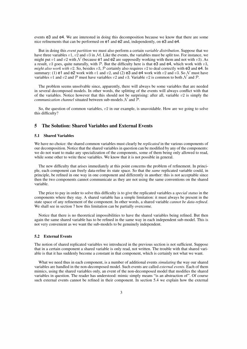
The development of this short example can be summarized in the following diagram. We first did a re-finement of our initial model M to M1 (thus preparing the interface), then we decomposed M1 intosub-models N and P , and finally we refined our two sub-models to NR and PR respectively:

M↓M1

↙ ↘N P↓ ↓NR PR

7 Another Example

The example presented in this section is a little less simple than the one presented in previous section.However, it is still clearly a bit artificial: we want to show how we can proceed in order to be able torefine the "natural" channel between two components. Contrarily to the previous example, we performseveral refinements on the non-decomposed model before eventually decomposing it. The goal of theserefinements is to construct carefully the interface between the future decomposed sub-models.

7.1 Initial Model

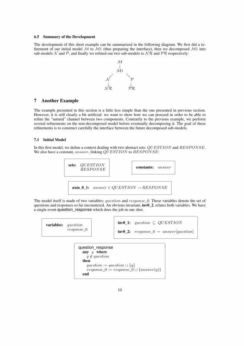
In this first model, we define a context dealing with two abstract sets: QUESTION and RESPONSE.We also have a constant, answer, linking QUESTION to RESPONSE:

sets: QUESTIONRESPONSE

constants: answer

axm_0_1: answer ∈ QUESTION →RESPONSE

The model itself is made of two variables: question and response_0. These variables denote the set ofquestions and responses so far encountered. An obvious invariant, inv0_2, relates both variables. We havea single event question_response which does the job in one shot.

variables: questionresponse_0

inv0_1: question ⊆ QUESTION

inv0_2: response_0 = answer[question]

question_responseany q where

q /∈ questionthen

question := question ∪ {q}response_0 := response_0 ∪ {answer(q)}

end

10

7.2 First Refinement

In this refinement, we introduce a channel, channel_0, between the sets question and response. Thesingle event of previous abstract model is split into two events named prepare_question and pro-duce_response. The former refines the abstract event question_response, while the latter is a newconvergent event (with variant the finite set channel_0). Notice that abstract variable response_0 isdata-refined to variable response with an obvious gluing invariant as shown in inv1_2.

variables: questionresponsechannel_0

inv1_1: channel_0 ⊆ question

inv1_2: response_0 = response ∪ answer[channel_0]

inv1_3: finite(channel_0)

prepare_questionrefines

question_responseany q where

q /∈ questionthen

question := question ∪ {q}channel_0 := channel_0 ∪ {q}

end

produce_responsestatus

convergentany q where

q ∈ channel_0then

channel_0 := channel_0 \ {q}response := response ∪ {answer(q)}

end

variant1: channel_0

At this point, it might be tempting to decompose this refinement into two sub-models with the sharedvariable channel_0 in between them:

channel_0question response

We shall not do that however because our intention is to later consider that channel_0 is a simple abstrac-tion for a far more complicated middleware component. In other words, we want to be able to later refinechannel_0. The idea is to encapsulate channel_0 in its own component so that the decomposition willbe as shown in the following figure:

responsequestion?

channel?

The purpose of the next refinements is to prepare the yet unknown interfaces between these components.

11

7.3 Second Refinement

In this refinement, we introduce a buffer, buffer_2 on the right hand side of the channel channel_0,which is data-refined to channel_1 (with gluing invariants inv2_1 and inv2_2). The buffer is controlledby the boolean variable bool_2.

variables: questionresponsechannel_1buffer_2bool_2

inv2_1: bool_2 = TRUE⇒ channel_0 = channel_1

inv2_2: bool_2 = FALSE⇒ channel_0 = channel_1 ∪ {buffer_2}

inv2_3: bool_2 = FALSE⇒ buffer_2 /∈ channel_1

prepare_questionany q where

q /∈ questionthen

question := question ∪ {q}channel_1 := channel_1 ∪ {q}

end

produce_responsewhen

bool_2 = TRUEwith

q = buffer_2then

bool_2 := FALSEresponse := response ∪ {answer(buffer_2)}

end

A new convergent event read_question is introduced (with variant the finite set {bool_2,TRUE}).

read_questionstatus

convergentany q where

q ∈ channel_1bool_2 = FALSE

thenbool_2 := TRUEchannel_1 := channel_1 \ {q}buffer_2 := q

end

variant2: {bool_2,TRUE}

7.4 Third Refinement

Similarly to what has been done in the previous refinement, we introduce now a buffer on the left handside of the channel.

12

variables: questionresponsechannelbuffer_1bool_1buffer_2bool_2

inv3_1: bool_1 = TRUE⇒ channel_1 = channel

inv3_2: bool_1 = FALSE⇒ channel_1 = channel ∪ {buffer_1}

inv3_3: bool_1 = FALSE⇒ buffer_1 /∈ channel

prepare_questionany q where

q /∈ questionbool_1 = FALSE

thenquestion := question ∪ {q}bool_1 := TRUEbuffer_1 := q

end

write_questionstatus

convergentwhen

bool_1 = TRUEthen

bool_1 := FALSEchannel := channel ∪ {buffer_1}

end

read_questionany q where

q ∈ channelbool_2 = FALSE

thenbool_2 := TRUEchannel := channel \ {q}buffer_2 := q

end

produce_responsewhen

bool_2 = TRUEthen

bool_2 := FALSEresponse := response ∪ {answer(buffer_2)}

end

variant3: {bool_1,FALSE}

7.5 Fourth Refinement

In this refinement, we introduce alternating bits as we did in the previous example.

13

variables: questionresponsechannelbuffer_1buffer_2bit_11bit_12bit_21bit_22

inv4_1: bit_11 ∈ {0, 1}

inv4_2: bit_12 ∈ {0, 1}

inv4_3: bit_11 = bit_12 ⇔ bool_1 = FALSE

inv4_4: bit_21 ∈ {0, 1}

inv4_5: bit_22 ∈ {0, 1}

inv4_6: bit_21 = bit_22 ⇔ bool_2 = FALSE

prepare_questionany q where

q /∈ questionbit_11 = bit_12

thenquestion := question ∪ {q}bit_11 := 1− bit_11buffer_1 := q

end

write_questionwhen

bit_11 6= bit_12then

bit_12 := 1− bit_12channel := channel ∪ {buffer_1}

end

read_questionany q where

q ∈ channelbit_21 = bit_22

thenbit_21 := 1− bit_21channel := channel \ {q}buffer_2 := q

end

produce_responsewhen

bit_21 6= bit_22then

bit_22 := 1− bit_22response := response ∪ {answer(buffer_2)}

end

7.6 Decomposition

At this point, we are now ready to perform our decomposition according to the following schemata:

question

buffer_1

bit_11

bit_12responsechannel

buffer_2

bit_21

bit_22

14

Left Component.

variables: questionshared: buffer_1

bit_11bit_12

invL_1: question ⊆ QUESTION

invL_2: buffer_1 ∈ QUESTION

invL_3: bit_11 ∈ {0, 1}

invL_4: bit_12 ∈ {0, 1}

prepare_questionany q where

q /∈ questionbit_11 = bit_12

thenquestion := question ∪ {q}bit_11 := 1− bit_11buffer_1 := q

end

external_write_questionwhen

bit_11 6= bit_12then

bit_12 := 1− bit_12end

Right Component.

variables: responseshared: buffer_2

bit_21bit_22

invR_1: response ⊆ RESPONSE

invR_2: buffer_2 ∈ QUESTION

invR_3: bit_21 ∈ {0, 1}

invR_4: bit_22 ∈ {0, 1}

external_read_questionany q where

q ∈ QUESTIONbit_21 = bit_22

thenbit_21 := 1− bit_21buffer_2 := q

end

produce_responsewhen

bit_21 6= bit_22then

bit_22 := 1− bit_22response := response ∪ {answer(buffer_2)}

end

Middle Component.

15

variables: channelshared: buffer_1

bit_11bit_12buffer_2bit_21bit_22

invM_1: channel ⊆ QUESTION

invM_1: buffer_1 ∈ QUESTION

invM_2: bit_11 ∈ {0, 1}

invM_3: bit_12 ∈ {0, 1}

invM_4: buffer_2 ∈ QUESTION

invM_5: bit_21 ∈ {0, 1}

invM_6: bit_22 ∈ {0, 1}

write_questionwhen

bit_11 6= bit_12then

bit_12 := 1− bit_12channel := channel ∪ {buffer_1}

end

read_questionany q where

q ∈ channelbit_21 = bit_22

thenbit_21 := 1− bit_21channel := channel \ {q}buffer_2 := q

end

external_prepare_questionany q where

q ∈ QUESTIONbit_11 = bit_12

thenbit_11 := 1− bit_11buffer_1 := q

end

external_produce_responsewhen

bit_21 6= bit_22then

bit_22 := 1− bit_22end

Appendix

As announced in section 5.4, the proof that the re-composition is indeed a refinement of the original non-decomposed model is now proposed here. We first present the mathematical framework, then we statewhat we have to prove, and finally we prove it. Note that the proofs presented in this Appendix have beenperformed automatically on the Rodin Platform.

We suppose that the initial non-decomposed model M has a state constructed on a set S. We areconcerned with an event e mathematically represented by a binary relation from S to S:

e ∈ S↔ S

For simplifying things without loss of generality, we envisage the decomposition of modelM into twosub-models N and P only. These two sub-models have states constructed on two sets T and U respec-tively.

The decomposition is materialized by means of two projections functions p and q from S to T and S toU respectively. These functions are total surjections:

16

p ∈ S � T

q ∈ S � U

The reason for these functions to be total surjections is that in a more concrete setting p and q are compo-sitions of proper Cartesian product projections prj1 and prj2, which are both total surjections.

The event e of modelM is projected on the two sub-models. This results in two events mathematicallyrepresented by two binary relations a and b:

a ∈ T ↔ T

b ∈ U ↔ U

These relations are the projections of relation e. They are formally defined as follows:

a =̂ p−1 ; e ; p

b =̂ q−1 ; e ; q

The sub-model N is refined to a model NR with a state constructed on a set X . The refinement is doneby means of a total binary relation l from X to T . Likewise, the sub-model P is refined to a model PRwith a state constructed on a set Y . The refinement is done by means of a total binary relation m from Yto U :

l ∈ X ←↔ T

m ∈ Y ←↔ U

These relations are assumed to be total: it is a fundamental assumption used in the refinement theory aspresented in chapter 14 of the book on Event-B.

Events a and b are refined to events ar and br. The forward refinement of these events is mathematicallyrepresented by the following predicates:

l−1 ; ar ⊆ a ; l−1

m−1 ; br ⊆ b ; l−1

Again, these refinement conditions come from chapter 14 of the book on Event-B (forward refinement).

The recomposition of refinementsNR and PR results in a modelMR whose state is constructed on aset Z. This set is projected on the two sets X and Y by means of two total surjective projections functionsu and v:

u ∈ Z � X

v ∈ Z � Y

We now re-compose an event er on modelMR

er ∈ Z↔ Z

by means of the two events ar and br. The event er is formally defined as follows:

er =̂ (u ; ar ; u−1) ∩ (v ; br ; v−1)

17

Here we construct the re-composed event er out of the existing refinement events ar and br. This is thereason why we used an intersection.

Putting together the two refinement relations l and m, we get a refinement relation n:

n ∈ Z←↔ S

which is defined as follows:

n =̂ (u ; l ; p−1) ∩ (v ; m ; q−1)

Relation n is indeed a total relation as both relations u ; l ; p−1 and v ; m ; q−1 are total. For example,u ; l ; p−1 is total because u is a total function, l is total relation, and p is a surjective function (hence p−1

is total relation).

All this can be illustrated on the following diagram:

YZX

ar er brl n m

u v

a e b

p q

u v

p qn ml

T S U

Now, we have to prove the following theorem stating that er is a refinement of e, that is:

n−1 ; er ⊆ e ; n−1

The proof is made of two parts. First, we prove:

n−1 ; er ⊆ r

and then we prove:

r ⊆ e ; n−1

where r is a relation from S to Z (as are both relations n−1 ; er and e ; n−1):

r ∈ S→ Z

defined as follows:

r = (p ; p−1 ; e ; p ; l−1 ; u−1) ∩ (q ; q−1 ; e ; q ; m−1 ; v−1)

18

Proof of the First Part. The proof of the first part can be conducted in a completely algebraic form.

PROOF

n−1 ; er= definition of ern−1 ; ((u ; ar ; u−1) ∩ (v ; br ; v−1))⊆ set theory(n−1 ; u ; ar ; u−1) ∩ (n−1 ; v ; br ; v−1)⊆ lemmas(p ; l−1 ; ar ; u−1) ∩ (q ; m−1 ; br ; v−1)⊆ refinements of a and b(p ; a ; l−1 ; u−1) ∩ (q ; b ; m−1 ; v−1)

= definitions of a and b(p ; p−1 ; e ; p ; l−1 ; u−1) ∩ (q ; q−1 ; e ; q ; m−1 ; v−1)

The previous proof relies on two lemmas. Here is the proof of the first one (the second one is similar).

PROOF of lemma: n−1 ; u ⊆ p ; l−1

n−1 ; u= definition of n((p ; l−1 ; u−1) ∩ (q ; m−1 ; v−1)) ; u⊆ set theory(p ; l−1 ; u−1 ; u) ∩ (q ; m−1 ; v−1 ; u)

= u is a total surjection(p ; l−1) ∩ (q ; m−1 ; v−1 ; u)⊆ set theoryp ; l−1

Proof of the Second Part. We have to prove now the second part, namely:

(p ; p−1 ; e ; p ; l−1 ; u−1) ∩ (q ; q−1 ; e ; q ; m−1 ; v−1) ⊆ e ; n−1

This proof cannot be conducted in an algebraic form like we did for the first part in the previous section.We have first to expand it as follows:

∀s, z′ · (∃s1, s1′ · p(s) = p(s1) ∧ s1 7→ s1′ ∈ e ∧ u(z′) 7→ p(s1′) ∈ l) ∧

(∃s2, s2′ · q(s) = q(s2) ∧ s2 7→ s2′ ∈ e ∧ v(z′) 7→ q(s2′) ∈ m)⇒(∃s′ · s 7→ s′ ∈ e ∧ u(z′) 7→ p(s′) ∈ l ∧ v(z′) 7→ q(s′) ∈ m)

We have now to be more precise about the sets S, T , U , X , Y , and Z. This can be done by means of thefollowing definitions:

S =̂ S1× S2× S3

T =̂ S1× S2

U =̂ S2× S3

X =̂ Z1× S2

Y =̂ S2× Z3

Z =̂ Z1× S2× Z3

19

As can be seen, the interface between the two sub-models N and P is played by the set S2. We can alsosee that S2 is not refined by looking at the definitions of sets X and Y .

The projections p, q, u, v are instantiated accordingly:

p(s1 7→ s2 7→ s3) = s1 7→ s2

q(s1 7→ s2 7→ s3) = s2 7→ s3

u(z1 7→ s2 7→ z3) = z1 7→ s2

v(z1 7→ s2 7→ z3) = s2 7→ z3

As a consequence, the predicates p(s) = p(s1) and q(s) = q(s2) (seen in the expansion of the state-ment to prove above) become p(s1 7→ s2 7→ s3) = p(s11 7→ s12 7→ s13) and q(s1 7→ s2 7→ s3) =p(s21 7→ s22 7→ s23) respectively. Now these predicates can be simplified to s1 = s11 ∧ s2 = s12 ands2 = s22 ∧ s3 = s23 respectively.

For instantiating the refinement relations l, m, and n, we introduce two relations λ and µ:

λ ∈ Z1× S2←↔ S1

µ ∈ S2× Z3←↔ S3

Next are now the instantiations of the refinement relations l, m and n:

(z1 7→ z2) 7→ (s1 7→ s2) ∈ l =̂ (z1 7→ z2) 7→ s1 ∈ λ ∧ z2 = s2

(z2 7→ z3) 7→ (s2 7→ s3) ∈ m =̂ (z2 7→ z3) 7→ s3 ∈ µ ∧ z2 = s2

(z1 7→ z2 7→ z3) 7→ (s1 7→ s2 7→ s3) ∈ n =̂ (z1 7→ z2) 7→ s1 ∈ λ ∧ (z2 7→ z3) 7→ s3 ∈ µ ∧ z2 = s2

Notice the various predicates z2 = s2. This takes account that the interface S2 is not refined.

It remains now for us to specialize the event e in two different ways.

First Specialization. First we consider a relation e2 leaving its component on set S3 unchanged, itis however modifying its components on sets S1 and S2. For this, we introduce a relation ε typed asfollows:

ε ∈ S1× S2↔ S1× S2

(s1 7→ s2 7→ s3) 7→ (s1′ 7→ s2′ 7→ s3′) ∈ e2 =̂ (s1 7→ s2) 7→ (s1′ 7→ s2′) ∈ ε ∧ s3 = s3′

This event e2 is typically the event a_2_b used in the first example. Here is again what we had to provebefore the instantiations (we removed the external universal quantification):

(∃s1, s1′ · p(s) = p(s1) ∧ s1 7→ s1′ ∈ e ∧ u(z′) 7→ p(s1′) ∈ l) ∧

(∃s2, s2′ · q(s) = q(s2) ∧ s2 7→ s2′ ∈ e ∧ v(z′) 7→ q(s2′) ∈ m)⇒(∃s′ · s 7→ s′ ∈ e ∧ u(z′) 7→ p(s′) ∈ l ∧ v(z′) 7→ q(s′) ∈ m)

Let us instantiate these three predicates in turn. The instantiation of:

20

∃s1, s1′ · p(s) = p(s1) ∧ s1 7→ s1′ ∈ e ∧ u(z′) 7→ p(s1′) ∈ l

is

∃s11, s12, s13, s11′, s12′, s13′ ·s1 = s11 ∧ s2 = s12 ∧(s11 7→ s12) 7→ (s11′ 7→ s12′) ∈ ε ∧ s13 = s13′ ∧(z1′ 7→ z2′) 7→ s11′ ∈ λ ∧ z2′ = s12′

That is:

∃s11′ · (s1 7→ s2) 7→ (s11′ 7→ z2′) ∈ ε ∧ (z1′ 7→ z2′) 7→ s11′ ∈ λ

The instantiation of:

∃s2, s2′ · q(s) = q(s2) ∧ s2 7→ s2′ ∈ e ∧ v(z′) 7→ q(s2′) ∈ m

is

∃s21, s22, s23, s21′, s22′, s23′ ·s2 = s22 ∧ s3 = s23 ∧(s21 7→ s22) 7→ (s21′ 7→ s22′) ∈ ε ∧ s23 = s23′ ∧(z2′ 7→ z3′) 7→ s23′ ∈ µ ∧ z2′ = s22′

that is

∃s21, s21′ · (s21 7→ s2) 7→ (s21′ 7→ z2′) ∈ ε ∧ (z2′ 7→ z3′) 7→ s3 ∈ µ

Finally, the instantiation of:

∃s′ · s 7→ s′ ∈ e ∧ u(z′) 7→ p(s′) ∈ l ∧ v(z′) 7→ q(s′) ∈ m

is

∃s1′, s2′, s3′ ·(s1 7→ s2) 7→ (s1′ 7→ s2′) ∈ ε ∧ s3 = s3′ ∧(z1′ 7→ z2′) 7→ s1′ ∈ λ ∧ z2′ = s2(z2′ 7→ z3′) 7→ s3′ ∈ µ ∧ z2′ = s2

That is:

∃s1′ · (s1 7→ s2) 7→ (s1′ 7→ z2′) ∈ ε ∧ (z1′ 7→ z2′) 7→ s1′ ∈ λ ∧ (z2′ 7→ z3′) 7→ s3 ∈ µ

So that we have to prove the following:

(∃s11′ · (s1 7→ s2) 7→ (s11′ 7→ z2′) ∈ ε ∧ (z1′ 7→ z2′) 7→ s11′ ∈ λ ∧(∃s21, s21′ · (s21 7→ s2) 7→ (s21′ 7→ z2′) ∈ ε ∧ (z2′ 7→ z3′) 7→ s3 ∈ µ)⇒(∃s1′ · (s1 7→ s2) 7→ (s1′ 7→ z2′) ∈ ε ∧ (z1′ 7→ z2′) 7→ s1′ ∈ λ ∧ (z2′ 7→ z3′) 7→ s3 ∈ µ)

yielding:

(s1 7→ s2) 7→ (s11′ 7→ z2′) ∈ ε ∧ (z1′ 7→ z2′) 7→ s11′ ∈ λ) ∧(s21 7→ s2) 7→ (s21′ 7→ z2′) ∈ ε ∧ (z2′ 7→ z3′) 7→ s3 ∈ µ)⇒(∃s1′ · (s1 7→ s2) 7→ (s1′ 7→ z2′) ∈ ε ∧ (z1′ 7→ z2′) 7→ s1′ ∈ λ ∧ (z2′ 7→ z3′) 7→ s3 ∈ µ)

The result is obtained by instantiating s1′ with s11′.

21

Second Specialization. Now we specialize the event e by considering a relation e1 leaving its componenton sets S2 and S3 unchanged: this event is just modifying its component on set S1:

(s1 7→ s2 7→ s3) 7→ (s1′ 7→ s2′ 7→ s3′) ∈ e1 =̂ s1 7→ s1′ ∈ ε ∧ s2 = s2′ ∧ s3 = s3′

This event e1 is typically the event in_a used in the first example. A treatment similar to the one we havedone for e2 leads to the following to prove:

(∃s11′ · s1 7→ s11′ ∈ ε ∧ (z1′ 7→ z2′) 7→ s11′ ∈ λ ∧ s2 = z2′) ∧(∃s21, s21′ · s21 7→ s21′ ∈ ε ∧ (z2′ 7→ z3′) 7→ s3 ∈ µ ∧ s2 = z2′)⇒(∃s1′ · s1 7→ s1′ ∈ ε ∧ (z1′ 7→ z2′) 7→ s1′ ∈ λ ∧ (z2′ 7→ z3′) 7→ s3 ∈ µ ∧ s2 = z2′)

yielding:

s1 7→ s11′ ∈ ε ∧ (z1′ 7→ z2′) 7→ s11′ ∈ λ ∧ s2 = z2′ ∧s21 7→ s21′ ∈ ε ∧ (z2′ 7→ z3′) 7→ s3 ∈ µ ∧ s2 = z2′⇒∃s1′ · s1 7→ s1′ ∈ ε ∧ (z1′ 7→ z2′) 7→ s1′ ∈ λ ∧ (z2′ 7→ z3′) 7→ s3 ∈ µ ∧ s2 = z2′

The result is obtained by instantiating s1′ with s11′.

22