An extended finitely recursive process model for discrete event systems

1616

xtended Finitely Recursive Process For Discrete Event Systems

Supratik Bose and Siddhartha Mukhopadhyay, Member, IEEE

Abstruct-In the area of Discrete Event Systems (DES) a grow- ing need is being felt for new classes of models to describe both logical and timed behaviors efficiently. Among the frameworks presented recently, the Finitely Recursive Process model is a powerfill one. However it is solely based on a characterization of the event strings generated in the DES. In this work an augmented version of the above model is presented, where the notion Of a collection of system related variables, forming the ‘state-space’ of the system, is introduced. A concept of a ‘silent transition’ is introduced for effective modelling of concurrent DES. To allow nonuniqueness of the initial state, an process framework is presented and a recursive characterization is made in terms of a collection of constant processes and process operators. A general Timed Transition Model (OStmff, 1990) is modelled as an extended process to show the describing power of the framework. A model of a robot controller is presented to show the usefulness of its different features in modelling real systems.

existing modelling tools from the field of computer science. Notable among them are Finite State Machines (FSM) [I], petri Nets (pN) [21, communicating sequential processes (CSP) 1319 Calculus of Communicating Systems (CCS) [4], Timed Transition Models ( n M ) [5] and Finitely Recursive Processes (I?”) [6]. Programming languages such as Ada and Occam, as well as simulation languages suchas GPSS, Simula etc., have also been used often for simulating and controlling such systems. Each formalism has its own merits and draw- backs. Moreover, in this early stage of development of the field, it is difficult to evaluate the various approaches in the field comparatively. Therefore, we shall only mention below the different features of each formalism briefly to indicate their bearing On

0 FSM. It is a simule and well understood model and the behavior Of DES.

I. INTRODUCTION

ISCRETE Event Systems (DES), their modelling, analysis, observation and control are receiving increasing

attention in the last decade. Such systems have been nearly always manmade. Therefore, quite naturally, as manmade systems grow in size and complexity, need arises to evolve a systematic and consistent theory to design, operate and evaluate them. Examples of such systems include Manufacturing Systems, Chemical Processes, Traffic Systems, Communi- cation Networks, Robotic Systems etc. Such systems are characteristically asynchronous, event driven, often nondeterministic or admit ‘choice’ of events by some unmodelled mechanism (environment). They are often modular and made up of distinct subsystems that evolve concurrently and with interactions in the form of interlocks, communication via channels or shared physical variables. The collection of these variables include numeric continuous variables such as a liquid level, numeric discrete variables such as machine parts in a buffer, or non-numeric variables such as traffic lights, relay flags or valve positions. Primarily the logical behavior of the systems, namely the sequence of events that occurs, is of interest. Structural properties such as liveness, reachability etc. often need to be assessed or ensured by proper design. Furthermore, often these systems are required to meet ‘hard’ real-time deadlines.

It is indeed difficult to capture all these features of DES efficiently in a single model. Attempts have been made to use

Manuscript received March 5, 1993; revised January 21, 1994, and October

generates a regular language. Many standard control concepts like controllability, observability , stabilizability and decentral- ized control have been studied in the context of this model. The main advantage of the FSM is that all t es like boundedness, deadlock freedom etc., are decidable in this framework. But practically, even for a simple physical system the state space may become very large and the description unwieldy.

0 PN. It is probably the most well known model for DES. Like FSM, PN can also model concurrency and nondeterminism. It generates the set of context sensitive languages. Recently some control theoretic properties have also been studied for PN. However the PN formalism lacks modularity, satisfactory verification techniques and a recursive characterization such that difficulty arises in automating the analysis for infinite state reachability graphs.

0 CSP and CCS. These algebraic process models provide a rigorous mathematical description for concurrent and communicating systems. They have inspired wide research in algebraic specification, verification and synthesis of concurrent and communicating systems, parallel programming languages etc. While the formalism of CSP allows nondeterminism, the CCS is inherently nondeterministic. These are able to model a Turing Machine (TM) and generate the set of recursively enu- merable (RE) languages. But the price paid for this describing power is the resultant undecidability of many issues [7].

0 FRP. It is a generalization of deterministic CSP. The major advantageous feature of FRP is its modular and recw- sive description through many operators. However it cannot

23, 1994.

Instltute of Technology, Kharagpnr, W.B 721302 India.

represent system related information effectively. Control issues are yet to be explored in this model. The FRP is also able to model a TM and as a result many issues become undecidable.

The authors are with the Department of Electrical Engineering, Indian

IEEE Log Number 9414494.

0018-9472/95$04.00 0 1995 IEEE

BOSE AND MUKHOPADHYAY EXTENDED FINITELY RECURSIVE PROCESS MODEL 1617

0 TTM. It is a state based framework specifically designed to model real time properties of DES. It admits the use of tem- poral logic as a specification language. It uses programming language features like variables, assignments, send, receive and guarded commands. Timed behavior is manifested through lower and upper time bounds of transitions. Proof theoretic techniques exist for verifying controller properties. But it lacks the feature of recursion. Further, modular process building is restricted since only parallel composition of individual TTMs is possible.

The motivation behind this work emerged from the recog- nition that both the events and the collection of system variables are independent real entities and therefore need to be modelled. While the FRP attempts to capture the dynamics in terms of the events, the TTM is solely concerned with state transformations. An important step in this direction has been taken through the suggestion of the notion of extended processes in [8], where both events and state transformations are dealt with simultaneously. However only a restricted class of operators, to be used for recursive definition, have been mentioned. Moreover possibility of shared variables among

Events: Let be a fixed finite collection of events and C* be the set of all finite length strings, called traces, including the null string ( ). C(C*) is the family of prefix closed subsets of c*.

Marks: By 'marking' is implied an assignment of values to a set of related mathematical objects after some event has taken place. This, in turn, determines the immediate future of the system. Each such assignment is called a 'mark'. Let M be a fixed set of marks, and 9 be a fixed family of functions from C* into M so that p E 9 A s E C* + p / s E 9 where

Marked Process: The Cartesian product W(C, M , 9) := C(C*) x K€J is called an embedding set. An element w = (tr w,pw) E W ( C , M , 9 ) (or simply W if there is no confusion) is called a marked process having tr w E C ( C * ) as its set of traces and pw E 9 , p w : tr w + M is the marking function so that pw(s) is the marking of the trace s.

Post process: If w E W and s E t r w, the post process of w after s is a process that captures the future behavior of the process w after the occurrence of the string s , and is denoted as w/s. It is defined as follows.

p / s ( t ) := p ( s A t ) , t E c*.

subprocesses and different constraints that may arise due to them have not been discussed.

In this paper we have presented the following enhancements over [8].

1) A global collection of variables, forming the basis Of

a global state space, is introduced that incor- porates variable sharing. Such variables may include a clock for modelling real time behavior.

tr(w/s) := {tls"t E t r w}, p(w/s)(t) := pw(sAt).

Embedding space: It is a triple (W, C, { r n} ) where W = W ( C , M , 9) is an embedding set, C is a partial order on W, and { 1' n, 72 2 0 ) is a family of projections mapping W onto itself that satisfies certain general properties. We are interested in a deterministic embedding space where for any E w,

2) A large collection of operators has been presented that can be used for complex recursive process description.

3) Several constraints have been suggested for the operators to be well defined for meaningful variable sharing and state continuity.

4) The concept of a silent transition has been introduced. This, it has been shown, is quite useful to depict situations where event dynamics is likely to be affected by transformations in shared variables.

Besides providing a theoretical exposition that aims to establish consistency of modelling rules for the processes and operators, it has been demonstrated that the Extended FRP can model a given TTM. Additionally, the example of a robot controller brings out the usefulness of various operators in modelling real world systems.

The paper has been organized as follows. Section I1 provides a brief mathematical background. Section I11 introduces the augmented version of FRP and its various features. In Section IV an extended process space is developed from the augmented FRP to encompass state dependent dynamics. In Section V the TTM framework and a robot controller have been modelled to serve as examples. Section VI concludes the work with directions for future research.

11. MATHEMATICAL BACKGROUND

w r 0 := HALT,.

where m := pw(()), tr (HALT,) := { ( ) } , p , HALT, (0) := m. The partial order is defined by: w C v iff t r w C t r v and pw(s) = pv(s),Vs E t r w. Then it is easy to check that w1 C w2 C ... converges to w where t r w = U; t r w, and for any i ,s ,pw(s) = pw;(s) if s E t r w n tr wz. The projection operator is defined as follows.

tr(w T n) = { s E t r wl#s 5 n}. p(w r n ) ( s ) = pw(s).

Here #s denotes the length of the string s. Marked Process Space: It is any subset (II, C, (1' n} ) (of-

ten denoted by II only) of an embedding space (W, c , { r n}) satisfying the following four axioms.

1) Axiom of projection: P E 11 + P 1' n E II,Vn 2 0. 2) Axiom of post-process: P E II and s E t r P + P / s E

3) Axiom of prefixing: Let R, PI, P2, . . . , Pk in IT be such II.

that

then

The ideas and definitions presented in this section are after [8]. They are presented for the sake of easy reference only. The reader is urged to go through [8] for detailed exposition.

4, Axiom Of completeness: If the p1 E: p2 . . . in IT converges to P in II then P E IT.

1618 IEEE TRANSACTIONS ON SYSTEMS, MAN, AND CYBERNETICS, VOL 25, N O 12, DECEMBER 1995

Elements of 11 are called (marked) processes. Any subset of II that satisfies the above axioms is called a process subspace.

Given a process space II = (II, C, (t n}), a process operator F: II - II is said to be

o continuous if for every chain Pl C P2 C ... in I I ,F(Pl ) C F(P2) C . . . is also a chain and u, F(P,) =

o constructive (con) if 'dP E 11 and n 2 0 F ( P ) t n + l =

o nondestructive (ndes) if 'dP E II and n 2 O,F(P)

The properties of continuity, con, ndes are preserved under composition of functions. Furthermore, if F is con and G is ndes then F o G and G o F are both con. We shall provide instances of such functions in the next section.

We end this section with the following theorem that specifies the conditions for unique solution of recursive equations defined on processes.

Theorem 2.1: Let II be a process space and consider the recursive equation

F ( U n Pn).

F ( P 1' n) 1' n + 1.

n = F ( P 1' n) 1' n.

P = F(P, U ) (1)

where F = (F1,F2,...,Fn): II" x IIk -+ II" and U = (U1,. . . , U k ) E IIk are given along with a set of consistent initial conditions

P , l ' O = Z o , = F , ( Z o l , ' ~ . , Z ~ n , U ) t o , i = l , - . . n . (2)

(CI) Existence: If each F, is continuous and ndes in P, then the process z = UI, zk is well defined where

Zo := (Z01,...,Zon), 2"' = F ( Z k , U ) , k 2 0.

Also 2 is the minimal solution of (l), (2) i.e., if P satisfies (l), (2) then 2, 5 P, for all i. Moreover this minimal solution is continuous, con, ndes in U, accordingly, as F is continuous, con, ndes in U,.

(C2) Uniqueness: If F is constructively guarded, Le., there do not exist indices 2 1 , . . . , i,, with i, = il such that F,, is not con in P,ie+l, 1 5 IC < m. Then (l), (2) have a unique solution.

Proo? See [SI.

111. AUGMENTED FINITELY RECURSIVE PROCESSES The process space described in the last section gives a

mathematical framework to describe the logical behavior of DES in terms of the traces. In this section we introduce a specific marked process space, called augmented process space, and a collection of operators that tries to capture different features of real world DES efficiently. Here the FRP of [6] is augmented with an explicit state transition function. The process space and operators presented here have many similarities as well as some important differences with the 'Deterministic Processes of Inan-Varaiya with memory' presented in [8].

We define a process space II which is a subspace of the deterministic embedding space W. The set of marks is

characterized by

M := 2' x (0, l} x Q

where, Q is the set of states. It is characterized in terms of a collection of variables, namely V . With each variable v E V , associated is a set, namely type(v), from which IJ takes values. The underlying state-space Q is defined as

Q := x type(v).

v E v. Note that, unlike [SI, the state space is constituted with fixed number of variables and is included in the mark. So any process P E 11 shares the same global state-space with other processes defined in II. However an individual process may actually access and manipulate only a subset of this set of variables. Therefore there will exist, in general, variables which are exclusive to a process as well as others shared among two or more processes.

Moreover, here C includes a special silent event X which may take place in a process only in response to events taking place in the 'environment' of the given process. We defer a detailed discussion on the features and role of X to the part on parallel composition operator later in this section.

Any process P = (tr P , p P ) E II satisfies the following marking axioms:

1) tr P E C(C*) , i.e., it is a prefix closed language and ( } E tr P.

2) p P ( s ) = (aP(s) , r P ( s ) , qP(s)) . Here aP: tr P + 2' is the alphabet function with aP(s ) denoting the set of events the process P can engage in (i.e., execute or block) after the occurrence of the event string s. The termination function rP: t r P + (0, l} denotes whether the process has successfully terminated after generating s (,P(s) = 1) or not. qP: t r P - Q is the state-transition function with qP( s ) denoting the state after s. Naturally m, qP( ( )) is the initial state.

3) s"(a) E tr P =+ a E aP(s) . 4) (s*t E t r P A T P ( s ) = I) 5) qP(s"(a)) = hF(s,qP(s)) , where h:: tr P x Q - Q

denotes the effect of the occurrence of the event o on Q in the process P after s has taken place. The above relation actually holds good only if the global state space is affected by the process P only and not by any other agent simultaneously. In such a situation, in fact, the whole treatment of state trajectories can be made in terms of q P ( . ) only, without introducing hr at all. However cases arise where other processes also independently affect the state along with P. In such a situation it becomes necessary to use the state transition function of P as well as those of other agents. This fact is explained while defining the parallel composition operator. It is for the same reason that both arguments of h:, namely, s and q, are necessary. Note that, as defined here, a process can have only a unique initial state. This is a severe restriction which causes several constraints on the various process operators defined later

t = ( ) .

BOSE AND MUKHOPADHYAY: EXTENDED FINITELY RECURSIVE PROCESS MODEL 1619

in this section. This restriction has been removed by introducing the extended process framework in the next section.

Now we describe a collection of constant processes and

o STOP and SKIP: the constant processes. The process STOPB,, E II is defined as: t r STOPB,, :=

operators to build up complex processes from simpler ones.

{( )};"STOPB,q(( )) := B;TSTOPB,q(( )) := 0;@=OPI3,,(( )) := 4 .

The process SKIPB,, E II is defined as: t r SKIPB,, := {( )};~SKIPB,,(( )) := B;TSKIPB,,(( )) :=

STOPB,, and SKIPB,, are nothing but Halt(B,O,q! and Halt(B,l,,), respectively, where Halt, has been defined in the earlier section. Physically STOPB,, and SKIPB,, denote the deadlocked process and the successfully terminated process at state q , respectively, from where no event is possible.

1;&KIPB,q(( )) := 4 .

o Local Change Operator (LCO): This operator has been introduced in [6] and an augmented

0 Given B , C 5 C and the process P, the LCO P[-B+C]

t r P[-B+C1 := { s E t r PJ i f Q is the first event of s ,

version is presented here.

is defined as

then Q $! B } *P[-B+C]( ( )) := (aP( ( )) - B ) u c;

~ P [ - ~ + ~ ] ( S ) := C u ~ ( s ) for s # ( ). .P[-B+Cl(S) := 7P(s ) ; Q P [ - ~ + ~ ] ( S ) := q ~ ( s ) for s E t r P [ - ~ + ~ ] .

o Global Change Operator (GCO): This also has been introduced in [6] and the augmented

0 Given B, C C and process P, the GCO P[[-B+c]l is version is presented here.

defined as

t r P [ [ - ~ + ~ ] ] := 1s E t r Plif 0 is any event in s ,

then 0 $! B} ,p[[-B+CIl ( s ) := ( a ~ ( s ) - B) u G for s E t r P [ [ - ~ + ~ ] ] ,P[[-B+C]l(s) := rP(s ) ;

gp[[-B+Cl] := qp(s) for E t r p[[-B+Cll.

The above two operators are used to remove traces from a process as well as change the blocking capability of the process while in parallel composition (defined later). It is easy to see that LCO and GCO are both continuous and ndes.

o State Modification Operator (SMO): Given some P E II ,r: Q + Q such that q P ( ( ) ) E Dr

(domain of T ) , the SMO, denoted by P{ r } , modifies the initial state and consequently the state trajectory of a process. It is defined as follows:

0 E t r PI,) and qP-lrH0) I= +P(O)). 0 If s E t r P{r} then ~ " ( 0 ) E t r P{r} iff s"(a) E

qP{r } (sA(0 ) ) := h% qP{r}(s ) ) . t r P A hF(s ,qP{r}(s)) is defined.

0 Vs E trP{r},aP{r}(s) := aP(s),.P{r}(s) := .rP(s). Clearly it is continuous and ndes.

o Deterministic Choice Operator (DCO): 0 Given A & C,T E { O , l } , q E Q,{Pl,..-,P,} G

II, { a l , . . . , a,} C A, (a, # a3 for i # j ) and respective transition functions hat: Q -+ Q , 1 5 i 5 n, the deterministic choice operator P = (a1 -+ PI 1 . . . la, + P,)A,~,, is defined as follows:

If T = 1 then P := SKIPA,, else

t r P := {( )} U { ( u . ) " s l s E t r P,>.

.P(( )) :=o, rP((a,)"s) := TP,(S).

qP(( )) := 4 , qP((a2)"s) := !7P,(s).

n

2=1

aP(( )) :=A, aP((a,)"s) := aP,(s).

The continuity of state is achieved under the following constraints: i) ha,(q) is defined for all i, ii) @,(( )) = ha,(q). Note that h: (( ), 0) = hat (0) but if a, is the last event of some string (a3)"s"(a,), then h ~ ( ( a , ) " s , 0 ) = h 2 ( s , 0 ) . The DCO describes the many courses of events that are possible at the beginning of a process. It also makes recursive equations guarded guaranteeing unique solutions. The DCO is continuous and con in each of its arguments.

o Sequential Composition Operator: (SCO) 0 Given Pl, P2 E II, the sequential composition P =

0 tr PI; P2 := AU B where A and B are defined as follows: PI; P2 is defined as follows:

A := {s E t r PlI(TPl(s) = 0) V ( ~ P l ( s )

B := { s = r"tl(r E t r P I ) A (TPI (T) = 1) A (qPl(r) = 1 A qPl(s) # qP2(( )I>}.

= !7P2(( ))) A (t E t r P2)).

Now observe the following: i) A n B = 4, ii) For any s E B , s can be broken up uniquely as s = rsAt, where r , and t , satisfy the conditions of r and t mentioned in definition of B .

0 a(Pl;P2)(s) := ( a P ~ ( s ) if s E A)v(aPz(t , ) if s E B). 0 7(P1;P2)(s) := (0 if s E A) v ( ~ P z ( t , ) if s E B ) . 0 q(Pl;Pz)(s) := (qPl(s) if s E A) V (qP2(t,) if s E B).

Thus PI; P2 initially behaves as Pl. After PI terminates successfully, if final state of PI matches with unique initial state of P2 then P2 starts operation. However if there is a mismatch then PI ; P2 deadlocks. Thus successful initiation of P2 in PI; P2 requires that the state after every successful termination of PI must uniquely match with the initial state of P2. This is again a constraint that arises due to the unique initial state granted to a process. The SCO contributes to modularity in description as well as increasing language complexity. It is continuous and ndes in each of its arguments.

o Parallel Composition Operator (PCO): It is in the definition of this operator that the augmented

process differs most from that in [6]. The difference emerges due to the introduction of the silent event X The PCO captures the concurrent evolution of two or more processes. Synchro- nization of certain tasks is brought about by naming the two tasks in the two processes identically. Such synchronous events appear only once in the trace. At times when one process generates an event 0, the other process may execute

1620 IEEE TRANSACTIONS ON SYSTEMS, MAN, AND CYBERNETICS, VOL 25, NO 12, DECEMBER 1995

X synchronously, irrespective of the event in the environment, but only n appears in the trace. This is explained below in detail.

0 At first we define inductively the projection of a string s E C* on a process P as follows:

i) ( ) l P := ( ) , ii) for n # A, s " ( n ) l p

(undefined if s l p @ t r P ) ( s l p " ( a ) if n E a P ( s l p ) ) ( s l p A ( X ) if n e a P ( s L p )

and X E a P ( s l p ) ) ( s l p if n, X $ aP(s1p) ) .

(undefined if s l p @ t r P )

( s l p if X 6 a P ( s l p ) ) .

.-

.- 1 iii) s " ( X ) l p := ( s l p A ( X ) if X E a P ( s l p ) ) { 0 Given processes PI , PZ the PCQ P = PI llP2 is defined

0 tr P is given inductively as: (a) () E t r P. (b) If s E t r P and q = qP(s) then ~"(a) E t r P iff the

alphabet condition: n E a P l ( s l p ) U aP2(slp2). trace condition: s " ( a ) l p % E t r P,, i = 1,2 . state condition(s): For n # A, i) If (s"(a)Lp, , s * ( o ) l p , ) = (sLp~"(n),sLp,"(X)) then

as follows.

following holds:

h,p"(sJ-~, , h? ( s ~ P ? , 4 ) ) and h p (SIP,, h?(s lp%, q ) ) are both defined and equal, for i , J = 1 , 2 ; i # j .

ii) Same as i) with X replaced by n. iii) Same as i) with n replaced by A. iv) For n including X if ( s A ( n ) l p , , s A ( n ) l p 3 ) =

(slp,"(a), SIP,) then h 7 ( s l p , , 4)) is defined for i,j =

Thus an event n # X can take place in a component process provided it is not blocked by the environment. Events common to the alphabets of the component processes must occur synchronously. If an event is possible in PI and is not blocked by P2 and at the same time the silent transition X is possible in P2, then n in PI and X in P2 will take place synchronously and only n will appear in trace of Pl lip2. Note that this occurs even if X is in the alphabet (and trace) of Pz. Essentially X has been introduced to model the fact that at certain points in the dynamics of processes, some change in the state variable, by events occurring in other external processes operating in parallel, may spontaneously cause a change in the event dynamics. By spontaneous we imply one without any deliberate action by the process itself or external manifestation. A typical analogy is that of a hardware interrupt where an event (interrupt) by another processor can simply

1 , 2 ; i # j .

cause a change in the event dynamics (jump to the interrupt service subroutine) without any external manifestation. Note that just as an interrupt can be disabled, a similar effect can be achieved by not including X in the alphabet. Further use of X will be found in the context of an extended process in Section IV. Though according to the definition, one may not always be able to block independent occurrences of X in traces of P1llPz, meaningfully, X should appear in traces of PlIIP2 only when it is acting as a component process in (PI I I Pz) 1 1 P3 for some P3 and X is induced in Pl/lPz by some event in P3. This meaningful behavior can be achieved by using GCQ [[-{A}]] on the process P describing the physical behavior of the overall system.

0 aP(s) := aP1(s lp l ) u aP2(s lp2) . 0 ~ P ( S ) := I if rP1(sLpl) = rP2(s lp2) = I

or ~ P z ( s l p ~ ) = 1 A (aP1(s lp l ) C aPz(slp,)) or

otherwise. Thus PI llP2 terminates if both terminate simultaneously or

if one terminates and blocks all the events that are possible in the other.

0 qP(( )) := qPl(( )) = qPz(( )). (See constraints of PCO). For a including X if qP(s) = q and ~"(0) E t r P then for 2, j = 1,2 ; i # j , (continued at the bottom of the page) The constraints that must be satisfied are: i) qP,(( )) = qPz(( )). This is because PI and Pz should have same initial global state for a well defined P1llP2. ii) All the function compositions used in finding qP(s) must be commutative. We emphasize here that this requirement is both natural and reasonable from the point of view of deterministic modelling of real world DES. Recall that either events are physically synchronous or they are modelled as such because their exact order of occurrence is deemed to be unimportant for the particular application of the model. In the former case commutativity is physical while in the latter only because it is satisfied, the events are modelled to be synchronous. Note that we do not require that the set of variables accessed and manipulated by the components of PCQ are disjoint as in [3] where the commutativity requirement is obviated. In case neither of the situations hold, loss of commutativity results in nondeterminism in the state trajectory. Since in this paper we concern ourselves with a deterministic framework, the commutativity of maps has been assumed to remove the possible nondeterminism when shared events modify common variables. iii) For any component process P,,X E aP,(s lpt) + s l p , * ( X ) E tr P,. To see the importance of this constraint, assume it is violated for some s and PI with sip% E t r P,. Then 'dn,slp2*(n) E t r P2 and n a P l ( s l p , ) implies s " ( n ) 6 tr(P1llPz). This is physically absurd. Note further, as far as the state dynamics is concerned, PllP # P. This equality holds in the case

T S ( S l p , ) = 1 A ( & z ( ~ l p , ) C aPi ( s lp , ) ) and 0


of CSP and FRP where the concept of state is absent. In AFRP also, tr(P1JP) = t r P. However even with simple state transition functions such as hF(.,q) = q + 1 with q E Z, h: ( s lp , h : ( s lp , 4)) # h : ( s l p , 4). Like SCO, PCO is also continuous and ndes in both its arguments.

Given an extended process P and a partial function T : Q -+

Q,P{T} is defined as follows:

DP{r) := ( 4 DPI (p (q ) ) { r ) is defined in the of an augmented process}.

P{THd := (P(q)){r l . We now proceed to extend the augmented FRP presented above.

IV. EXTENDED FINITELY RECURSIVE PROCESSES Instead of providing a recursive characterization of the

augmented process space I T , we first extend it to characterize the extended process space llQ. The motivation behind going for an extended process space are as follows.

* In II explicit state dependent decisions (branching) cannot be modelled.

* Elements of II are defined to have unique initial states. This imposes constraints on operator definitions and their applicability to real systems.

The extended process space and its components are defined first.

Definition 4.1: The extended process space corresponding to lI and Q is defined as

IIQ := {PIP: Q + IT is any partial function.}

o Assignment Operator (AO): Given a partial function h: Q --+ Q and an extended process

P , the A 0 P[h] is given as:

Pbl: Q + ITIP[hl(q) := P(h(q)); DP[h] := { q E Dhlh(q) E D P }

This operator is widely used for satisfying the state continuity constraint in DCO of extended processes as evident from the examples provided later in this paper.

Note the difference between ESMO and AO. In the former, the initial state of the augmented process P(q), i.e., qP(q)(( )), gets modified to r(qP(q)(( ))) and the subsequent state trajectory also changes. In the latter, the argument of the extended process P changes from q to h(q) and a new augmented process P(h(q)) gets selected.

o Extended DCO: (EDCO) Given extended processes P I , . . . , P,, distinct events

( P ( d / S ) if s E tr(P(q)) undefined otherwise.

Note that D(P/s"\t) C D(P/s ) C D(P) .

tors { 1' n} on IIQ are induced from those on II as follows: Definition 4.3: The partial order (C_) and projection opera-

Vn(P 1' n)(q) :=P(q) 1' n and D ( P 1' n) = DP. P R iff D P = DR and P(q) R(q)

for all q E DP.

The 'constant' extended processes and process operators in

STOP and SKIP the constant (extended) processes: 0 STOPp,: Q --t IT has D(STOPp,) = Q, and

0 SKIPB: Q t ll has D(SKIPB) = Q, and S K I P B ( ~ ) :=

o Extended LCO: (ELCO)

IIQ are defined as follows.

S T O P B ( ~ ) := STOPB,,.

SKIPp,,,.

p[-B+C]: Q -+ ITlp[-B+Cl(q) (P(q))[-B+C1;

Dp[-B+C] := DP.

o Extended SMO: (ESMO)

p ( q ) := (ak + P k ~ ( q ) I ' * ' lak, Pk,(q))A(q),r(q),q'(q)

where {kl,. . . , k t } = { j l q E DPj A hu3 (4) is defined}. Also w is a partial function satisfying v(q) = (A(q), ~ ( q ) , q'(q)) + for all kl , (state continuity). D P := { q E Qlv(q) is defined and 4 # {ukl, . . . ,ak,} C A(q) and state continuity is satisfied}. We denote u just by A , T if Vq E DP,w(q) = (A, T, 4). Note that we use the same symbol for both process operators as well as their extended versions. If the initial marking (function) w is dropped, then Vq E DP,v(q) = ({al,...,u,},O,q) . Also the notation (a1 + ... a, + P ) actually denotes (al -+ (a2 -+ (. . . (a , -+ P) . . .))). Then it is straightforward to observe that every extended process has a one-step extension:

{ak, , . ' . , ak, } E A(q). Further, q(pk, ( q ) ) ( ( )) = ha,l ( q ' (4 ) )

P := [a1 4 P / ( U l ) l . . . la, -+ P / ( a n ) l v

where

{ ( a d , . . . , ( G J } = u {s E t rP(q) l#s = 11 q € D P

and the partial function 21 is defined as w (4) : = p P ( q ) ( ( )) . o Extended SCO: (ESCO) Given extended processes P1 and P z , P = P I ; P2 has a

domain D(P1; P2) := DP1. For q E D(Pl ;Pz ) ,P l ; P2(q) is defined as follows:

1622 IEEE TRANSACTIONS ON SYSTEMS, MAN, AND CYBERNETICS, VOL. 25, NO. 12, DECEMBER 1995

e tr P I ; Pz( q ) := A u B where A and B are defined as

A := { s E t r Pl(q)l(TPl(q)(s) = 0 ) V ( ( ~ P l ( q ) ( s ) = 1) follows:

A ((4’ := 4Pl (d (S ) 6 DPz) v ( 4 / # 4Pz(4 / ) ( ( )))))}.

A (4’ := qPl(q)(T) E DP2) A (4’ = !TPz(40(( ))I A (t E tr P2(q’))).

B := { s = rAt l ( r E tr P,(q)) A (TPl(q)(r) = 1)

Now observe the following: i) AnB = 4. ii) For any s E B , s can be broken up uniquely as s = rSAts where r, and t , satisfy the conditions of r and t mentioned in definition of 3.

if s E B).

s E B ) . * dP1;Pz ) (q ) ( s ) := ( @ l ( d ( S ) if s E A) v ( @ Z ( Q ’ ) ( t S )

if s E B).

s E tr P l ( q ) , ~ p l ( q ) ( s ) = 1 and 4’ = @l(q)(s) ,Pz cannot start at q’ due to (4’ := qPl(q)(s) $2 DP2) V (q’ qPz(q’)(( ))) lhen P1;Pz deadlocks, i.e, Pl;P2(q) / s =

However state matching requirement for the initiation of the second process in SCO has been relaxed by letting Pa have variable initial state q’ and allowing the composition to deadlock only if state continuity fails to hold even after that.

a ( p l ; P z ) ( q ) ( s ) := (aPl(q)(s) if s E A)v(aP2(q’)(ts)

e T(Pl ;Pz ) (q ) ( s ) := (0 if s E A) V (.Pz(q’)(t,) if

Note that like SCO, in the extended case also, if, for some

STOPcyPl(4)(S),*“

o Extended PCQ: (EPCQ) Given extended processes P1 and Pz, P1 llPz is defined as

p = P1IIP2: (2 + HlP(q) := P1(q)IlP2(q), for q E DP where DP := { q E DPl fl DPalP1(q)llPz(q) is defined.}.

o Multiple Branching operator (MBQ): Given m binary valued Boolean conditions bo, . . . , b,-l

and 2m extended processes P O , , P p - 1 , the MBO

,bo)(Po,... ,P2--1):

Q ---t nIP(q) := Pr(q)

where r , 1 5 T 5 2” - 1, is the decimal equivalent of the binary number ( b m - l ( q ) . . . b ~ ( q ) ) with each b,(q) being 0 or 1 depending upon b,(q) is false or true respectively.

DP := { q E QI(b,-l(q) - b o ( q ) ) = T and q E DP,}.

The following property is satisfied by MBO:

((bm-1, ’ . , bo)(Po, = (bm-1 , . . . , bo)(PoIIR,. . . , P2--1/IR).

That is, within a parallel composition, if one component faces a logical branching, the branching will take place instanta- neously. This may however pose modelling difficulties as evinced in the following example.

Example 1: Let

p := (X = + P [ l){a},O> ( b + Pz[ R :=(e i P3[z = 1 =+ z := 0,z = 0 * 2 := l]){c],O.

Consistent with the definition of P , let it be desired that b should take place in P only from the state z = 0. Consider

the parallel composition of P and R at state 40 := (x =

P3[ ] ) { c } , ~ ( q ~ ) ) . In this process suppose the first event is c and it sets z := 1. At this state the event b is possible in the concurrent process even with the state z = 1. From the way P is defined, this is not desired. To prevent this kind of situation, without using Hoare’s restriction of disjoint variable sets, X can be helpful. What we want is that, since P shares variables with the environment and P faces a logical decision based on these global variables, actions in the environment should not go unnoticed by P . It should be able to reconsider its decision whenever there is a change of global state actions in the environment. Clearly, if P is modified to P’

0) . w e have PIIR(q0) := ( ( 6 + P2[ l ) { d - , o ( ~ o ) ) l l ( ( ~ +

P’ := (z = ())((a + p11 I IX + P’[ l){a,A},O> ( b + Pz[ IlX + P’[ I ) { b , A } , O )

then (P’llR)[[-{’}l](q~) will not have such problem. With the help of the above mentioned operators, we give

a recursive characterization of IIQ. As in [8], we define the following.

DeJinition 4.4: An operator F : (IIQ)k --+ IIQ is called a spontaneous operator if it is continuous and ndes in all its arguments and for any P I , . . . ,P I , in IIQ, F(P1 T 0 , 0 ) = F(P1 1‘ O,...,Pk T 0 ) 0.

Dejnition 4.5: A collection of operators r, is called a mutually recursive spontaneous (MRS) family of operators if every F : -+ IIQ in r is spontaneous and for any (P) E tr F ( P l , . . . , P k ) (where tr

and q E DF(P1,. . . , Pk) there exist Fi E r so that F(P1, . . ’ , Pk) := U q E D F ( p l , ,pk) tr(F(P1,. . . , P k ) ( d ) )

F(P1, . . ‘ , Pk)/(Oj ( 4 ) = q p / , , ’ . . , PA) ( 4 )

provided the left hand side is defined and where for each j , 1 5 j 5 m, there exist i, 1 5 i 5 k , such that

(Pi = P z ) v (Pi = P, / (a ) ) v (Pi = P, / (X) ) .

DeJinition 4.6: Given an MRS family of operators r,stn(r) is the smallest family of functions (US), + IIQ that satisfies the following:

1) For any B C_ C , r E (0, l}, the ‘constant’ functions STOPB and SKIPB E P(r) where STOPB (PI , . . . , P,) := STOPB and similarly for

2) For i = l , . . . , n Proj, E V(r) where

3) If F1,. . . , Fk are in S t n ( F ) and G in r maps i

It is easy to see that all functions in LY(r) are spontaneous because of preservation of spontaneity under function composition. Q(r) := U, Rn(I‘).

Dejinition 4.7: A finite set { P I , , P,} is called a family of mutually recursive extended processes (MREP) with respect to W(r) if for all j , P , , q E DP,, s E tr P, ( q ) , we have P,/s(q) = Fq(P1,...,P,)(q) for some Fq E Qn(r).

SKIPB.

Proji(P1,...,P,) := P,.

IIQ then G o ( F l , . . . ,Fk) E !?(I?).

BOSE AND MUKHOPADHYAY: EXTENDED FINITELY RECURSIVE PROCESS MODEL 1623

Theorem 4.1: {PI, . . . , P,} is MREP w.r.t P(r) if P = ( P I , . . . , P,) is the unique solution of the recursive equation

Y = F ( Y ) , Y 0 = P 0 (3)

where each component F, of F is guarded, i.e,

F,(P) = (azl + F,, (P)I * * [aikz --$ FZkZ (PI) (4)

where each F,, E W(F) and w,: Q + M is a suitable function.

Proofi Similar to the recursive characterization of II in [SI.

DeJnition 4.8: P E IIQ is called an extended FRP (EFRP) if for some n it can be expressed as X = F ( X ) , P = G ( X ) where X = X I , . . . , X,, F is of the form (4.2) and G E Rn(r ) . P is termed as EFRP since for any q E DP, s E t r P(q),P/s(q) can be expressed as

P/s(q) = Gs,(P)(q)

for some G,, E Q(r). Definition 4.9: The extended algebraic process with respect

to IIQ and R ( r ) is the collection A ( @ , Q) of all EFRPs. Now all that is needed is to specify explicitly in the

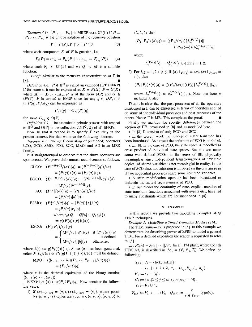
present context. For that we have the following theorem. Theorem 4.2: The set F consisting of (extended) operators

LCO, GCO, SMO, PCO, SCO, MBO, and A 0 is an MRS family.

It is straightforward to observe that the above operators are spontaneous. We prove their mutual recursiveness as follows:

ELCO : (P[-B+CI / ( a) ) ( 4 ) : = (P[--B+CI ( 4 ) ) / ( a )

= ( P ( d ) / ( a ) = P/(4)(d*

= (p/( ,))[[-B+C]l ( 4 ) .

= ( P / (4 1 IhI(4).

= (P/(4)r,(q),

:= Q((P(Q)){T})((d).

= { ( P ~ / ( a ) ) [ h ] ( q ) otherwise,

EGCO: (p[[-B+cll / (a ) ) (q ) := (P[[-B+cll ( 4 ) ) / ( 4

AO: (PIhl / (a))(q) = (P(h(q) ) / (a)

ESMO: (P{r ) l (a ) ) (q ) = ( P ( d ) { r ) / ( a )

where r,: Q + QIVij E Q,rq(q")

ESCO: (P1; P2) / (4 (4 ) (Pd(a ) ;P2) (4 ) if ( P l / ( d ) ( q )

is defined

where h(.) := q(Pl(.))(( )). Since ( a ) has been generated, either P l (q) / (a ) or P ~ ( q ( P l ( q ) ) ( ( ) ) ) / ( a ) must be defined.

MBO: ( ( L i , . . . , bo) (Po , . . . f'zn -1)/(a))(q)

= (PT/(d)(d where P is the decimal equivalent of the binary number

EPCO: Let ( a ) E tr(P1IIP2)(q). Now consider the follow- ( L l ( d , . . . 1 bo(Q)) .

ing cases. 1) If ( a ) l P l ( q ) = (Ol) , (+P&) = ( a 2 ) , where possi-

ble (a , al,a2) tuples are (a, a, a ) , (a, a, A), (a , X,a) or

(X,X,A) then

(P1 IIP2)/(.) ( 4 ) = I((Pl/ (a1 )) { h y ) 1) II ((Pd ( 0 2 ) ) {hb:' (4) > ) I ( 4 ) i

where

hLp(q)(.) := h?(,)(( ), .) for i = 1,2 .

2) For i , j = L2, i # j , if (4k(,) = (4, (4b3(*) =

( P Z I I P , ) / ( 4 ( d = [((Pz/(a))ll((P,){hbP~(P)})l(4),

( ), then

where hkp'(q)(.) = hbp'(q)( ( ), .). Note that here CT

includes X also. Thus it is clear that the post processes of all the operators

mentioned in r can be expressed in terms of operators applied on some of the individual processes and post processes of the

Finally we mention the specific differences between the

* In [SI r consists of only PCO and SCO. * In the present work the concept of silent transition has

been introduced. As a result the definition of PCO is modified. * In [8], in the case of PCO, the state space is modelled as

cross product of individual state spaces. But this can make some well defined PCOs, in the sense of [SI, physically meaningless since independent transformations of 'multiple copies' of shared variables is not meaningful in reality. In the case of SCO also, no restriction is imposed on the domain even if two sequential processes share some common variables.

* A state modification operator has been introduced to maintain the mutual recursiveness of PCO.

* In our model the continuity of state, explicit mention of state transition functions associated with events etc., have led to many constraints which are not mentioned in [SI.

others. Hence r is MR. This completes the proof.

version of IIQ introduced in [8] and as modelled here.

V. EXAMPLES

In this section we provide two modelling examples using

Example I : Modelling a Timed Transition Model (TIM). The TTM framework is proposed in [5]. In this example we

demonstrate the describing power of EFRP to model a general TTM. For a detailed exposition the reader is requested to refer to [5 ] .

. . . llM, be a TTM plant, where the i th TTM M , is described as M , = (V,, O,, 'L). We define the following:

EFRP techniques.

Let Plant =

T, := % - {tick, initial}

={~,~11 < j L k , ~ , = (ez3,hZ,,L,,~Z3). v, .=v, - (7).

C, := {czJ 11 I j I k , type(cZJ) = W. v, :=v, u c,.

1624 IEEE TRANSACTIONS ON SYSTEMS, MAN, AND CYBERNETICS, VOL 25, NO. 12, DECEMBER 1995

In the above description the plant is modelled as the parallel composition of n TTMs. An individual TTM is described as a tuple of a set of variables V,, an initial condition e,, and a collection of transitions x. Each transition 7 of x is a tuple consisting of an enabling condition e, a state transformation h, a lower time bound 1 and an upper time bound u. From x two special transitions, ‘initial’ and ‘tick‘, are removed to form T,, which now contains k , number of transitions. From V, the next transition variable 7 is removed and ki counter variables are added, one for each transition of the TTM, other than ‘tick’ or ‘initial’. We now deal with an extended variable set VEX and state space QEX . The central idea is to introduce an individual extended process for each transition of the ?rfM, which takes care of respective enabling conditions and time bounds using counter variables, silent transitions and MBO. These processes are called ‘event processes’. However ‘initial’ and ‘tick’ are modelled explicitly as events since they don’t have such constraints.

We now proceed to give the formal definition of the EFRP ‘Plant’ that models a general TIM ‘Plant’. It is formulated as a concurrent operation of n extended processes Mi, 1 5 i 5 n, each of which models the i th TTM M,.

At a state q, the realization M,(q) of the extended process M, either evaluates to a deadlocked process or it is ready to execute ‘initial’ and engage in purposeful activity, depending upon whether @,(q) is false or true. If it is false for some i then ‘Plant’ is deadlocked due to STOP{lnl,,al) in Mi. Otherwise ‘Plant’ starts meaningful activities with ‘initial’ taking place in all its components. Y, is a recursive process. In each call of Y, a parallel composition of k , ‘event processes’, namely IIP,, , 1 5 j 5 k,, is called. Once this composition terminates, Y, is called again.

Y, is modelled to be a nonterminating process since the TTM is such. The ‘event process’ Pz, plays the key role in modelling.

P,, = ( (ez3 , c,, < zZ3 , cZ3 < uZ3 )(x,,, , . . . , x ~ ~ ~ ) ) [ [ + { ~ ~ ~ ~ > ~ ~ J 111

ez3 :=

eZ3 if r,, is not a shared transition. ez131 A . . . A eZJi3& if rz3 is shared as

rzz131 , . . . , 7 i k 3 k in M,I . . . , M,k , respectively.

XZl0 = x,,, = x,32 = x, 3 3

:= (A + SKIP{ }[c,, : 0] ltick + SKIP{ 1 [t: t + I, c,, : 01)

XZl4 := (A + SKIP{ } [ ]IT,, + SKIP{ >[h,, , c,: 01)

XZJ5 : = ( A + SKIP{ I[ ] l t ick-+SKIP~}[t : t+1,c ,3: c,, +1]

17z3 + SKIP{ } [k) , CZ) : 01) XZJ6 :=arbitrary XZJ7 := (A + SKIP{ > [ ]

ltick -+ SKIP{ )[t: t + 1,cZ3: ct3 + 11) f h, if r? is not a shared transition.

\ . . . , M,k, respectively.

Now we explain the operation of the event process P,,. The process XZ,,,(= X,,, = X,,, = Xz3,) corresponds to the case when the enabling condition for rZ3 is false. At this stage, in P,,, only ‘tick’ or X (due to some 7 k l in some Pk,) is allowed. Also the counter is reset to zero. X,3,7 takes place when the enabling condition is true but the value of time is less than the lower bound. Here also the event rz3 cannot take place. However in response to ‘tick’, counter is incremented. The idea behind keeping X in each of these processes is to be able to check enabling as well as timing conditions after every event in the environment of P,, . However X is prevented from appearing in the traces of overall process ‘Plant’ using the GCO [[-{A}]]. X Z J 5 pertains to the case when the enabling condition, as well as both the lower and upper time bound constraints are satisfied and rZ3 is allowed to happen. Xz36 is left arbitrary as this case never arises under l,, 5 u,, . X,34 is the case when the counter value equals uz3. It is interesting to note that in this case ‘tick’ is not allowed as its occurrence will violate the upper time bound constraints of TTM. Physically this means that, before the next time instant, either T,~ will take place or the enabling condition will become false due to some event in the environment. The GCO [[+{tick,~23}]] ensures that ‘tick’ is synchronized among all processes and T , ~ is also synchronized when it is a shared transition. Communicating transitions are also modelled as shared transitions. Finally note that in each call of llpl E, llr=l( 11$1 P,,) terminates, its components terminating synchronously, either after a ‘tick’ in all the components, or rz3 in one (or some if shared) and X in others. In the next call (at a new state), all the conditions are rechecked. Thus ‘Plant’ models ‘Plant’ successfully.

Example II: Modelling a Robot Controller. In this section we develop the EFRP model of a robot

controller which carries out some repetitive work on a job depending upon the program selected. The basic actions of the robot controller are taken from an example in [SI. Briefly, the actions are as follows.

After ‘power on’ and ‘system initialization’ the robot enters in the ‘manual’ mode and its state is ‘inactive’. In this mode the program to be run can be selected and the valid command is ‘start’. In response to ‘start’ the state becomes ‘establishing connection’ where the controller sends repeated job requests to a scheduler. After a fixed number of requests if the job is not granted the robot gives a connection failure signal and goes back to manual mode. If granted, the robot enters the ‘working’ state and loads the selected program in the buffer. Each program is assumed to be a sequence of block


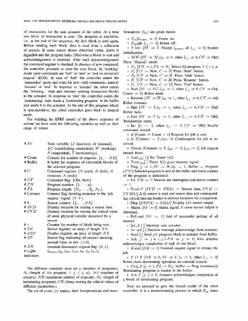
of instructions for the axis actuator of the robot. At a time one block of instruction is sent. The program is repetitive, i.e., at the end of the sequence, the first block is sent again. Before sending each block, data is read from a collection of sensors. If some sensor shows abnormal value, alarm is signalled and the program halts. Otherwise a block is sent and acknowledgement is received. After each acknowledgement the command register is checked. In absence of new command, the controller proceeds to send the next block. In ‘working’ mode valid commands are ‘halt’ or ‘end’ or ‘end on (external) request’ (EOR). In case of ‘halt’ the controller enters the ‘suspended’ mode and waits for new valid commands, namely ‘resume’ or ‘end’. In response to ‘resume’ the robot enters the ‘working ’ state and resumes sending instruction blocks to the actuator. In response to ‘end’ the controller enters the ‘terminating’ state, loads a ‘terminating program’ in the buffer and sends it to the actuator. At the end of this program which is non-repetitive, the robot controller goes back to manual mode.

For building the EFRP model of the above sequence of actions we have used the following variables as well as their range of values.

# SV

# Count # Buffer

# C

# CF # PN # P L # Connect

# k # SVD # CVD

# j # S R # DSP # S F

# D R # Light indicators

State variable: { I (inactive), M (manual), EC (establishing connection), W (working), S (suspended), T (terminating)}. Counter for number of requests: { 1, . . . N R } It holds the sequence of executable blocks of the selected program. Command register: { S (start), H (halt), R (resume), E (end)}. Command flag: {Old, New}. Program number: { 1, . . . , p } . Program length: { N I , . . . , Np , NT}. Connect flag showing response to the ‘job request’ signal: { T , F } . Sensor counter: { 1, . . . , N S } . Dummy location for storing a sensor data. Dummy location for storing the critical value of some physical variable measured by a sensor. Counter for number of block being sent. Sensor register, an array of length NS. Display register, an array of length NS. Sensor flag indicating all sensors showing normal value or not: (1, O} External disconnect request flag: { 0, l}. ~Power,lM,1EC,~CF,~W,~S,~T,~I.

The different constants used are p (number of programs), Ni (length of ith program, 1 5 i 5 p } , N S (number of sensors), N R (maximum number of requests), NT (length of terminating program), C R (Array storing the critical values of different parameters.).

The set of event (a) names, their interpretations and trans-

formations (h,) are given below.

* Pon[Zpower := 11 Power on. * Poff[all 1 0 := 01 Power off. * S-Init [SV := I , Except lpower, all I ( . ) := 01 System

* M M [SV := M , ~ M := 0, other l(.l := 0,CF := Old]

* P,, [PN := i , P L := N,] Select ith program. 1 5 i 5 p . * P, [CF := New, C := SI Press ‘Start’ button. * Ph [CF := New, C := HI Press ‘Halt’ button. * P, [CF := New, C := R] Press ‘Resume’ button. * P, [CF := New, C := E ] Press ‘End’ button. * Start [SV := EC, I E C := 1, other I ( := 0, C F := Old,

* Resume [SV := W, lw := 1, other l ( . ) := 0, C F := old]

* Halt [SV := S, ls := 1, other 1 0 := 0 ,CF := Old]

* End [SV := T,IT := 1, other Z(.) := 0 ,CF := Old]

* Inv [I1 := 1, other I ( ) := 0,CF := Old] Invalid

* Jr [Count := Count + 13 Request for job is sent. * Jc [Connect := T,IEc: 01 Confirmation for job is re-

* Discon [Connect := F,IEc := 0,IcF := 11 Job request

* Tsetl(2) [ I Set Timer l(2). * Tout1(2)[ ] Timer l(2) gives timeout signal. * Prog [j := 1,SV := W,lw := 1, Buffer := Program

(I“)] Selected program is sent to the buffer and block counter of the program is initialized.

* Int-S [k := 11 Sensors are interrupted and sensor counter := 1.

* Read-S [SVD := S R ( k ) := Sensor data, CVD := CVR(k)] Kth sensor is read and sensor data and corresponding critical data are loaded in dummy locations for comparison.

* Disp [DSP(k) := SR(k ) ] Display kth sensor output. * Alarm [SF := 01 Alarm signal, if some sensor output is

* Poll-end [SF := 11 End of successful polling of all

* Int-A [ ] Interrupt axis actuator. * Int-ack [ ] Receive interrupt acknowledge from actuator. * Send [ ] Send j t h program block to actuator from buffer. * Ack [ j := j + l ; j > PN j j := 11 Axis actuator

acknowledges completion of task of one block. * R-end [DR := 11 External request signal to release the

job. * E-0-R [DR := 0 , SV := T , ~ T := 1, other I ( := 01

Robot starts terminating operation on external request. * Prog-T [j := 1, P L := NT, Buffer := Prog (terminate)]

Terminating program is loaded in the buffer. * Ack-T [j: j + I] Actuator acknowledges completion of

a block of terminating program.

Now we proceed to give the formal model of the robot controller. It is a nonterminating process in which Po, starts

initialization.

Press ‘Manual’ mode.

Count := 01 Robot starts.

Robot resumes.

Robot halts.

Termination starts.

command sensed.

ceived.

turned down.

abnormal.

sensors.

1626 IEEE TRANSACTIONS ON SYSTEMS, MAN, AND CYBERNETICS, VOL. 25, NO. 12, DECEMBER 1995

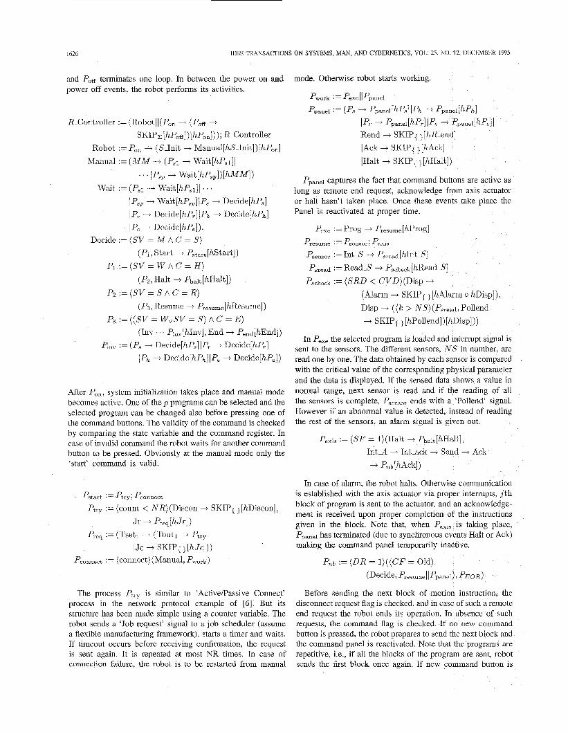
and P o ~ terminates one loop. In between the power on and power off events, the robot performs its activities.

R-Controller := (RobotII(Pon + (Po, --f SKIPclhPo~]) [hP,,])); R-Controller

Robot := Po, + (S-Init + Manual[hSlnit])[hPon] Manual := ( M M -+ (Psl i Wait[hPsl]I

. . . lPsp + Wait[hP,,])[hMM])

lPsp + Wait[hPsp]IPs -+ Decide[hP,] lP, + Decide[hP,]IPh -+ Decide[hPh] IP, -+ Decide[hP,]).

Decide := (SV = M A C = S)

Wait :=(PSI i Wait[hP,~]/

(PI, Start + Pstar,[hStart])

(Pz, Halt + Phalt [hHalt])

(P3, Resume + Presume [hResume])

(Inv ---f PI,, [ hInv] , End + Pend [ hEnd])

/Ph -+ Decide[hPh]IP, + Decide[hP,])

P i : = ( S V = W A C = H )

P2 := (SV = S A C = R)

P3 := ((SV = W”SV = S ) A C = E )

PI,, := (Ps + Decide[hP,]IP, -+ Decide[hP,]

After Po,, system initialization takes place and manual mode becomes active. One of the p programs can be selected and the selected program can be changed also before pressing one of the command buttons. The validity of the command is checked by comparing the state variable and the command register. In case of invalid command the robot waits for another command button to be pressed. Obviously at the manual mode only the ‘start’ command is valid.

Pstart := Ptry ; Pconnect

Ptry := (count < NR)(Discon -+ SKIP{ 1 [hDiscon],

Pres := (Tsetl --f (Tout1 -+ Ptry Jr + Preq[hJr])

IJc -+ SKIP{ } [ h J c ] ) ) Pconnect := (connect)(Manual, Pwork)

The process Ptry is similar to ‘ActivePassive Connect’ process in the network protocol example of [6]. But its structure has been made simple using a counter variable. The robot sends a ‘Job request’ signal to a job scheduler (assume a flexible manufacturing framework), starts a timer and waits. If timeout occurs before receiving confirmation, the request is sent again. It is repeated at most NR times. In case of connection failure, the robot is to be restarted from manual

mode. Otherwise robot starts working.

Pwork := PexeIIPpanel

Ppanei := (ps 4 ppanel [hPs] 1 P h -+ Ppanel [hPh] lP, -+ ppanel[hPr]/Pe + Ppanel[hPe]I Rend -+ SKIP{ 1 [hR-end] lAck + SKIP{ } [hAck] IHalt i SKIP{ 1 [hHalt])

Ppane1 captures the fact that command buttons are active as long as remote end request, acknowledge from axis actuator or halt hasn’t taken place. Once these events take place the Panel is reactivated at proper time.

Pexe := Prog -+ P r e s u m e [hprogl .-

P r e s u m e .- Psensor; Pam,

PsenSor := Int-S ---f Psread[hInt-S] Psread := R e a d 3 + Pscheck[hRead-S]

Pscheck := (SRD < CVD)(Disp -+

(Alarm 4 SKIP{ } [hAlarm o hDisp]), Disp + ( ( k > NS)(Psread,Pollend + SKIP( 1 [hPollend])[hDisp]))

In P,,, the selected program is loaded and interrupt signal is sent to the sensors. The different sensors, N S in number, are read one by one. The data obtained by each sensor is compared with the critical value of the corresponding physical parameter and the data is displayed. If the sensed data shows a value in normal range, next sensor is read and if the reading of all the sensors is complete, PsenSor ends with a ‘Pollend’ signal. However if an abnormal value is detected, instead of reading the rest of the sensors, an alarm signal is given out.

Paxis := ( S F = l)(Halt + Phalt[hHalt], Int-A + Int-ack + Send -+ Ack

+ Pnb[hAck])

In case of alarm, the robot halts. Otherwise communication is established with the axis actuator via proper interrupts, j t h block of program is sent to the actuator, and an acknowledgement is received upon proper completion of the instructions given in the block. Note that, when Pax,, is taking place, Ppanel has terminated (due to synchronous events Halt or Ack) making the command panel temporarily inactive.

Pnb := ( D R = 1) ( (CF = Old)

(Decide, P r e s u m e I I Ppanel) , PEOR)

Before sending the next block of motion instruction, the disconnect request flag is checked. and in case of such a remote end request the robot ends its operation. In absence of such requests, the command flag is checked. If no new command button is pressed, the robot prepares to send the next block and the command panel is reactivated. Note that the programs are repetitive, Le., if all the blocks of the program are sent, robot sends the first block once again. If new command button is

BOSE AND MUKHOPADHYAY: EXTENDED FINITELY RECURSIVE PROCESS MODEL

pressed, it proceeds to check the validity of the new command.

:= (Tseta t (Tout2 --f haltIP, t Decide[hP,] lP, Decide[hP,]IPh + Decide[hPh] lP, --f Decide[hP,]))

In the halt process a timer is set and the some command button to be pressed.

PE-O-R := (E-0-R -+ Pend[hE-O-R]) Pend := Prog-T + P,nt,[hProg-T]

controller waits for

Pintr := (IntA + Int-ack -+ Send -+ Ack-T -+ ( ( j > PL)(P,,t,,Manual))[hAck-T])

In the terminating procedure, the special terminating program is brought to the buffer and sent to the actuator blockwise. At the end of this procedure the robot goes back to the manual mode.

VI. CONCLUSION In the present work, the FRP framework presented in [6] has

been augmented and extended in several respects. A large class of operators have been used to give a recursive characterization of the extended process. However the present framework remains deterministic. Nondeterminism and hiding are the aspects that are currently being investigated. The following are some of the significant open problems for future work.

* Development of a specification mechanism for EFRP. ModalRemporal logic may be investigated.

* Development of verification techniques exploiting the recursive structure of EFRP.

* Development of Axiomatic proof rules for undecidable issues like liveness for EFRP.

* Controller synthesis from specification languages. * Observation and control under partial observation. All the above are theoretical issues. Probably, the acid test of

a modelling framework lies in its application to model the real world. Challenging large scale applications from fields such as power systems, manufacturing systems, communication networks etc. are therefore much needed to establish the efficiency, simplicity and describing power of many emerging modelling tools in DEDS.

ACKNOWLEDGMENT The authors thank Dr. Amit Patra of Department of Elec-

trical Engineering, I. I. T Kharagpur and the anonymous reviewers for many helpful suggestions regarding this work. The second author acknowledges the support under VGC Career Awards Scheme during the revision of the paper.

1627

REFERENCES

P. J. G. Ramadge and W. M. Wonham, “The control theory of discrete event systems,” Proc. ZEEE, vol. 77, no. 1, pp. 81-98, Jan. 1989. T. Murata, “Petri nets: Properties, analysis and applications,” Proc. ZEEE, vol. 77, no. 4, pp. 541-580, Apr. 1989. C. A. R. Hoare, Communicating Sequential Processes. New Delhi: PHI Pvt. Ltd., 1989. R. Milner, Communication and Concurrency. Hertfordshire, UK: PHI Ltd., 1989. J. S. Ostroff and W. M. Wonham, “A framework for real time discrete event control,” ZEEE Trans. Automat. Contr., vol. 35, no. 4, pp. 386-397, Apr. 1990. K. Inan and P. Varaiya, “Finitely recursive process models for discrete event systems,” ZEEE Trans. Automat. Contr., vol. 33, no. 7, UP. _ _ 626439, July 1988. R. A. Cieslak and P. Varaiva. “Undecidabilitv results for deterministic communicating sequential processes,” ZEEE Trans Automat. Contr., vol. 35, no. 9, pp. 1032-1039, Sept. 1990. K. Inan and P. Varaiya, “Algebras of discrete event models,” Proc. ZEEE, vol. 77, no. 1, pp. 24-38, Jan 1989. K. Nielsen and K. Shumate, Designing Large Real-Time Systems With Ada. New York Intertext Publicationshlultiscience Press Inc., Ch. 27, Appendix E, 1988.

I

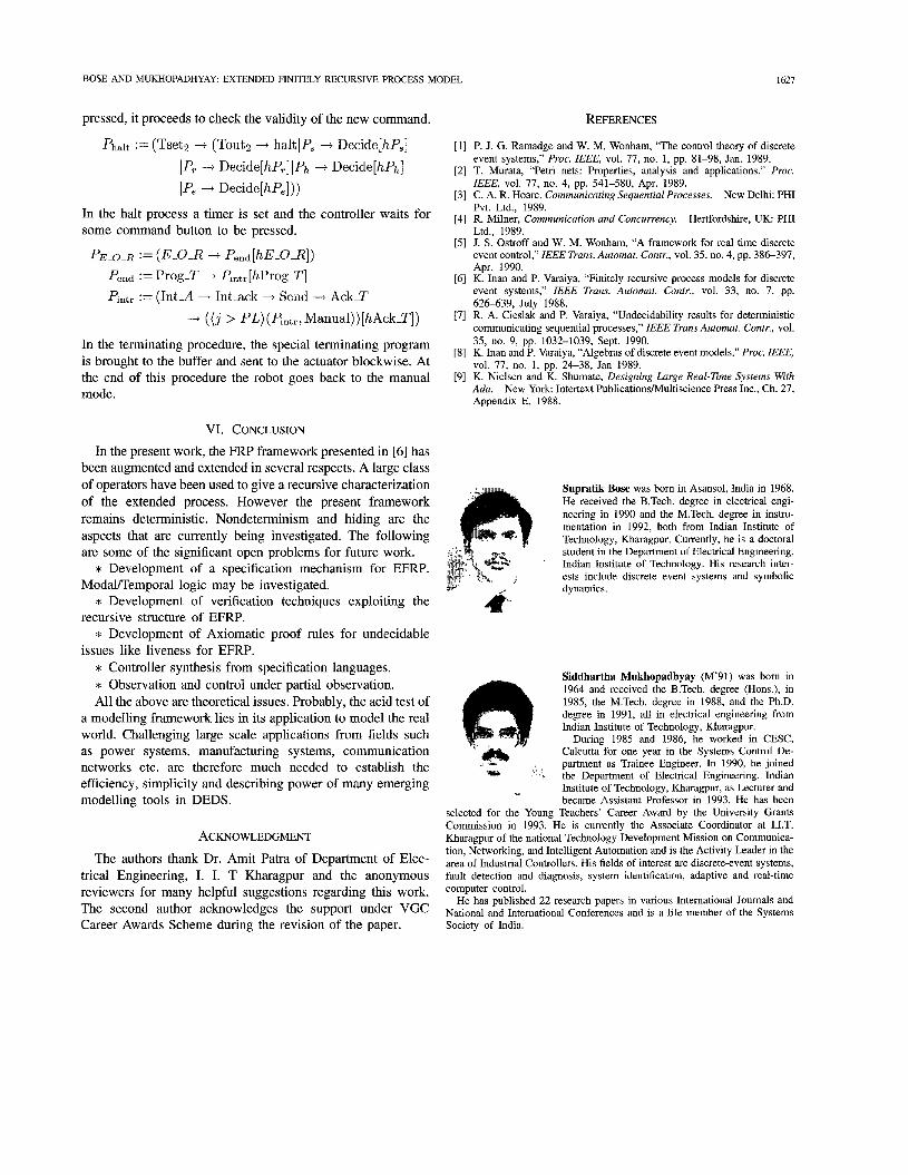
Supratik Bose was born in Asansol, India in 1968. He received the B.Tech. degree in electrical engineering in 1990 and the M.Tech. degree in instru- mentation in 1992, both from Indian Institute of Technology, Kharagpur. Currently, he is a doctoral student in the Department of Electrical Engineering, Indian Institute of Technology. His research inter- ests include discrete event systems and symbolic dynamics.

Siddhartha Mukhopadhyay (M’91) was born in 1964 and received the B.Tech. degree (Hons.), in 1985, the M.Tech. degree in 1988, and the Ph.D. degree in 1991, all in electrical engineering from Indian Institute of Technology, Kharagpur.

During 1985 and 1986, he worked in CESC, Calcutta for one year in the Systems Control De- partment as Trainee Engineer. In 1990, he joined the Department of Electrical Engineering, Indian Institute of Technology, Kharagpur, as Lecturer and became Assistant Professor in 1993. He has been

selected for the Young Teachers’ Career Award by the University Grants Commission in 1993. He is currently the Associate Coordinator at I.I.T. Kharagpur of the national Technology Development Mission on Communica- tion, Networking, and Intelligent Automation and is the Activity Leader in the area of Industrial Controllers. His fields of interest are discrete-event systems, fault detection and diagnosis, system identification, adaptive and real-time computer control.

He has published 22 research papers in various International Journals and National and International Conferences and is a life member of the Systems Society of India.

An extended finitely recursive process model for discrete event systems

Documents

Transcript of An extended finitely recursive process model for discrete event systems