Analytica Chimica Acta, 150 (1983) 71-86 Elsevier Science Publishers B.V., Amsterdam - Printed in The Netherlands

INTERACTIVE CALIBRATION BY A RECURSIVE GENERALIZED STANDARD ADDITION METHOD

BERNARD VANDEGINSTE*, JO KLAESSENS and GERRIT KATEMAN

Department of Analytical Chemistry, University of Nijmegen, 6525 ED Nijmegen (The Netherlands)

(Received 6th December 1982)

SUMMARY

The generalized standard addition method (GSAM) has recently been introduced for calibration to avoid matrix effects and many interferences. In GSAM, all additions and measurements precede the calculations of the K matrix (sensitivities of all analytes at all sensors) and the analyte concentrations. A recursive version of GSAM is presented here. Some new powerful properties are added to the method: (1) on-line checking of the validity of the linear model during the data acquisition stage, (2) simultaneous evaluation of the value and precision of the elements of the K matrix during the additions, and (3) access to an on-line interactive calibration, terminating the additions when the precision is within the desired limits or a deficiency in the model has been detected. The method is demonstrated for spectrophotometric measurements of copper and nickel in the presence of EDTA.

The quality of the calibration of most analytical methods fixes the quality of the final result. In most cases, there is no absolute quantitative relationship between analyte concentration and response (or reading), so that the response obtained for an unknown sample has to be compared with the responses obtained for a number of calibration samples. The problems associated with calibration are well known: the selectivity of many analytical sensors is poor, and many constituents present in the sample may affect the response, i.e., interfere. A second serious problem associated with calibration is the varying sensitivity of the sensor with changing matrix in the sample, i.e., the matrix effect. Of course, calibration methods which handle these problems adequately have been available for many years. Interferences may be compensated by applying a multi-component analysis. Matrix effects may be avoided by using the standard addition method.

Until very recently, systems where interferences and matrix effects occur simultaneously could not be calibrated in a direct way. The problem has been solved by combining the multicomponent analysis and the standard addition method [l, 21 into a widely applicable method, the generalized standard addition method (GSAM). The merit of GSAM is not only the assessment of calibration in a more general way, but also the provision of a quantitative relationship between the precision of the analytical result and

0003-2670/83/$03.00 o 1983 Elsevier Science Publishers B.V.

72

the measurement error, in relation to the design of the calibration. Therefore, GSAM constitutes a firm step toward a self-calibrating system, which will become of full value when the measured response is placed in a feedback loop with the progress of the experimental design. This means that each new step in the calibration stage is decided on the basis of all responses collected previously.

In its present form, GSAM does not provide this feature. All additions precede the calculations of the sensitivity constants (K matrix), the analyte concentrations and the propagated error in the result. This implies that there is no check that the underlying model remains valid during the additions. Equally, no indication is obtained on the necessity of further additions, taking into account the desired precision of the analytical result. For this purpose, an algorithm is needed which returns improved least-squares estimates of the model parameters (e.g., sensitivity coefficient), every time a new measurement has been acquired. Such a recursive algorithm opens the way to achieve a feedback between response and experimental design, which is essential in the development of self-calibrating systems. Very recently, the first applications of recursive algorithms in analytical chemistry have been reported [3-6] as an alternative to the calculation of the analyte concen- trations in a multicomponent procedure.

In this paper, a recursive version of the GSAM is presented, which adds some new powerful properties to the method: (1) on-line control of the validity of the model (linear) during the calibration stage; (2) simultaneous evaluation of the value and precision of the elements in the matrix of the sensitivity coefficients, during the additions; (3) access to an on-line inter- active calibration, terminating the additions, when either the precision is within the desired limits, or a deficiency in the model has been detected.

THEORY

For a clear understanding of the recursive GSAM, the underlying principles will be discussed stepwise by an outline of multicomponent analysis, the standard addition method, the generalized standard addition method (GSAM), and the recursive least-squares method, leading to the recursive generalized standard addition method (RGSAM).

Formulation of the analytical problem The problem is to determine the concentrations of NA analytes in a parti-

cular sample. Each of the NA anslytes contributes to the response measured at a particular sensor. On the assumption that the responses are additive, the response at sensor i can be expressed as

R, =y ki,c, + e, (1) J=l

73

where c, are the unknown concentrations, ei is the measurement noise, and hi, is the sensitivity coefficient of analyte j at sensor i.

At least NA independent measurements are required to determine all NA concentrations. The analytical problem then can be formulated as follows: given a mzasurement vector R of NS (NS > NA) independent sensors, and a matrix K of sensitivity coefficients, find the bestestimates i: of the true concentrations c from the response equation: R = K c + e, where R is a NS X 1 column vector of NS responses, c is a NA X 1 column vector of the un- known concentrations, e is a NS X 1 column vector of the measurement noise, and I? is a NS X NA matrix of the sensitivity coefficients.

Solution 1: Multicomponent analysis Under the very restricted condition that the sensitivity coefficients K are

independent of the matrix and the concentrations c, the solution of the analytical problem can be found simply by an ordinary multicomponent analysis. For NS > NA, the number of equations exceeds the number of un- knowns. A general solution method for such an overdetermined system of equations is the least-squares method that minimizes C e:, where ei represents the difference between the actual response Ri and the estimated response Ri, given by Eqn. (1). The solution is given by the well known generalized inverse

-- iZ = (KrK)-’ KTR (2)

The remaining problem is to quantify K by a calibration procedure, which in view of the afore-mentioned rest@tions can be kept very simple.

The condition of the matrix K [2] is the factor with which the measure- ment error may be amplified in the analytical result, where

Il~clI/llclI G ~~~~(~)[(ll~~IIIII~II) + (ll~RII/IIRII)l (3)

and I ICI I and I IKl I are the norms of the vector c and the K matrix, respectively. Although the ordinary least-squares method seems very attractive at first sight, a serious drawback becomes apparent when an extra measurement is made at a (NS + 1)th sensor. Of course, the solution of the problem is still given by Eqn. (2), but with one important distinction. Prior information is now available because an estimate 6 of the true concentration c is available. However, Eqn. (2) does not provide any means to use that information. Although algorithms which do take into account this prior information have been in use in other disciplines for some time, their applications in analytical chemistry are more recent [ 3,6] .

The general form of a recursive algorithm is: new estimate E = (known function of) old estimate + correction In terms of the above analytical problem, the “old” estimate is based on NS measurements, and the new one on (NS + 1) measurements. The value of the correction term depends on the information obtained from the last, (NS + l)th, measurement. Poulisse [3] clearly demonstrated that complex multi- component systems can be solved elegantly in this way, and explained the

74

mathematical background of recursive estimation methods, which will be summarized below in discussion of the recursive generalized standard addi- tion method.

Solution 2: Standard addition method Many multicomponent analyses are not easily calibrated, because the

sensitivity coefficients of the analytes depend on the constitution of the sample. In practice, the preparation of good standards, closely matched to the sample, is often very difficult or impossible, and this problem is often circumvented by calibrating directly in the sample, following the standard addition method. The response for a sample with NA analytes at sensor i is

R, = y k:jCj + ei J=l

When analyte 1 is added to the sample (under the condition of constant volume), the change in the response is

ARi = y ki,c, + ki,Acl + ei j=l

(5)

Further additions and calculation of the regression coefficient between ARj and AC, gives an estimate i7;‘1 of k:, . From Eqn. (4), however, it is clear that the concentration c1 of the first analyte in the sample can be calculated only if the other analytes do not contribute to the response (ki,(, _+ 1j = 0) and if there is no background. This means that the ordinary standard addition method yields reliable results only when the sensor is specific for the analyte measured.

Solution 3: Generalized standard addition method Difficulties arising from the lack of selectivity of the sensor when the

standard addition method is applied, can be overcome by adding standards of all NA analytes (sequentially or simultaneously) to the sample; this allows calculation of all sensitivity coefficients, kIj (j = 1, NA). Because the concen- trations of NA analytes are determined, responses at NS > NA sensors should be measured in order to obtain a solvable system. This is the basic principle of the generalized standard addition method (GSAM), developed by Saxberg and Kowalski [ 11. The method consists basically of two steps: (1) calibra- tion by adding standard solutions of all analytes and calculation of the sensitivity coefficients of all analytes at all sensors (K matrix); (2) calcula- tion of the analyte concentrations from the initial responses of the sample measured at all sensors. Details of the method and the mathematical expres- sions have been given [ 1, 21.

The generalized standard addition method is a powerful calibration tool. Many interferences and matrix effects can be handled by GSAM, so that

75

complex sample preparations can be avoided. In order to minimize the number of additions, and to ensure the validity of the calibration, the addi- tions should be stopped as soon as the sensitivity coefficients are known with sufficient precision, or when the assumed linear model between con- centration and response is no longer valid. This requires coupling of the experimental design with the outcome of the measurements during the calibration. The present form of GSAM does not provide these possibilities because results are evaluated only after completion of all additions.

Solution 4: Recursive generalized standard addition method The problem of the calibration at one sensor (i) will be discussed first.

For a sample with NA analytes, the initial response (before the additions) is

Because the numbers of moles are additive, instead of concentrations, volume-corrected responses and concentrations are introduced [ 21: Qi,, = RI,,& and nis = qsVo, where V, is the initial volume. Equation (6) then becomes

Qi,s = ki,ln,,, + ki,zn2,8 + ‘** + ki,NAniv,t,, + et

or in matrix notation

The vector of the sensitivity coefficients, b, will be determined in a recursive calibration procedure.

If all the analytes are added simultaneously in a single addition with a total volume Au, and the added number of moles of analyte i is An,, i then the change of the response at sensor i after the addition is

A&i = Ri(Vo + V) -Qi, = (Anl,l An,,, l ** AnI,& k,l k i, 2

.

0

= Anyk + e, .

k, N.4

In order to start the recursive estimation procedure for k, it is necessary to initialize-two parameters: (1) an estimate of the sensitivity coefficients, e.g., zero or k(0); and (2) an estimate of the precision of the estimates of the sensitivid coefficients. These estimates are the diagonal elements of the matrix P(0). The off-diagonal elements are set to zero. With AQi(l) in hand, a first estimate of the sensitivity coefficients can be obtained by applying the following recursive filter [ 31 :

k(1) = C(O) + g(1) [AQi(l) -AnT(l) C(O)]

g(1) = p(O) An(l) [e(l) + AnT(l) p<O) An(l)]-’

P(l) = p(O) -g(l) AnTP(0) (7)

76

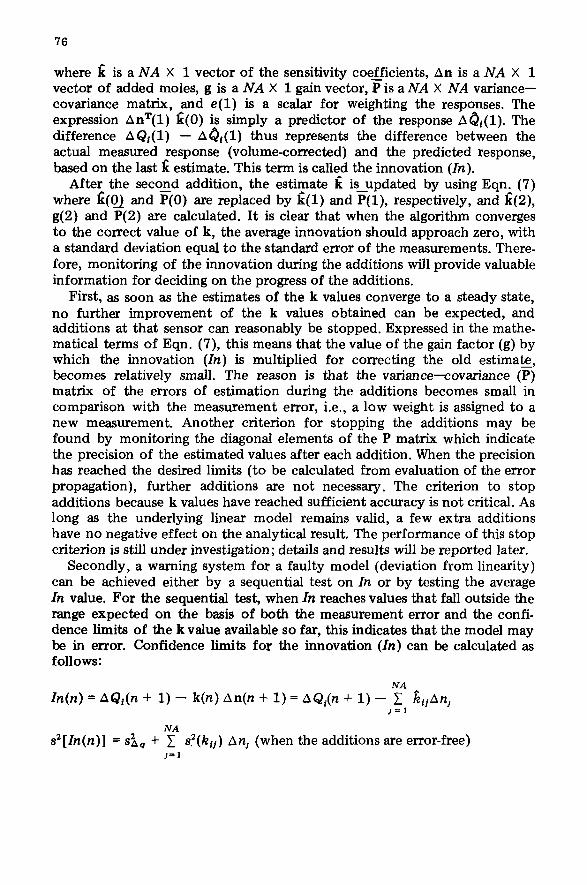
where k is a NA X 1 vector of the sensitivity coefficients, An is a NA X 1 vector of added moles, g is a NA X 1 gain vector, Pis a NA X NA variance- covariance matrix, and e(1) is a scalar for weighting the responses. The expression An=(l) k(0) is simply a predictor of the response A&l). The difference A Qi(1) - A&l) thus represents the difference between the actual measured response (volume-corrected) and the predicted response, based on the last k estimate. This term is called the innovation (In).

After_ the second addition, the estimate & is-updated by using Eqn. (7) where k(OJ and P(0) are replaced by k(1) and P(l), respectively, and k(2), g(2) and P(2) are calculated. It is clear that when the algorithm converges to the correct value of k, the average innovation should approach zero, with a standard deviation equal to the standard error of the measurements. There- fore, monitoring of the innovation during the additions will provide valuable information for deciding on the progress of the additions.

First, as soon as the estimates of the k values converge to a steady state, no further improvement of the k values obtained can be expected, and additions at that sensor can reasonably be stopped. Expressed in the mathe- matical terms of Eqn. (7), this means that the value of the gain factor (g) by which the innovation (In) is multiplied for correcting the old estimate, becomes relatively small. The reason is that the variance--covariance (P) matrix of the errors of estimation during the additions becomes small in comparison with the measurement error, i.e., a low weight is assigned to a new measurement. Another criterion for stopping the additions may be found by monitoring the diagonal elements of the P matrix which indicate the precision of the estimated values after each addition. When the precision has reached the desired limits (to be calculated from evaluation of the error propagation), further additions are not necessary. The criterion to stop additions because k values have reached sufficient accuracy is not critical. As long as the underlying linear model remains valid, a few extra additions have no negative effect on the analytical result. The performance of this stop criterion is still under investigation; details and results will be reported later.

Secondly, a warning system for a faulty model (deviation from linearity) can be achieved either by a sequential test on In or by testing the average In value. For the sequential test, when In reaches values that fall outside the range expected on the basis of both the measurement error and the confi- dence limits of the k value available so far, this indicates that the model may be in error. Confidence limits for the innovation (In) can be calculated as follows:

In(n) = AQr(n + 1) - k(n) An(n + 1) = AQ,(n + 1) - “; LijAn, J=l

s’[ln(n)] = & f y s?(k,) An, (when the additions are error-free) J=l

77

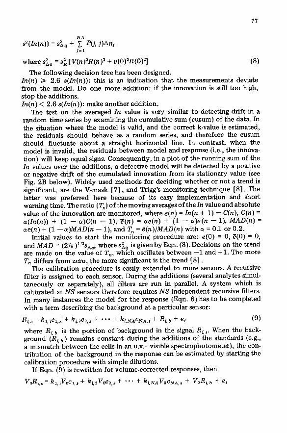
s”(ln(n)) = si, + y PCj, j)An, j=l

where s& = s; [ V(n)%(n)2 + u(O)%(O)2] (8)

The following decision tree has been designed. In(n) > 2.6 s(ln(n)): this is an indication that the measurements deviate from the model. Do one more addition: if the innovation is still too high, stop the additions. In(n) < 2.6 s(ln(n)): make another addition.

The test on the averaged In value is very similar to detecting drift in a random time series by examining the cumulative sum (cusum) of the data. In the situation where the model is valid, and the correct k-value is estimated, the residuals should behave as a random series, and therefore the cusum should fluctuate about a straight horizontal line. In contrast, when the model is invalid, the residuals between model and response (i.e., the innova- tion) will keep equal signs. Consequently, in a plot of the running sum of the In values over the additions, a defective model will be detected by a positive or negative drift of the cumulated innovation from its stationary value (see Fig. 2B below). Widely used methods for deciding whether or not a trend is significant, are the V-mask [7] , and Trigg’s monitoring technique [8]. The latter was preferred here because of its easy implementation and short warning time. The ratio (T,) of the moving averages of the In value and absolute value of the innovation are monitored, where e(n) = In(n + 1) - C(n), C(n) = cy(ln(n)) + (1 - a)C(n - l), Z(n) = ewe(n) + (1 - e)Z(n - l), MAD(n) = se(n) + (1 - a)MAD(n - l), and T, = E(n)/MAD(n) with (Y = 0.1 or 0.2.

Initial values to start the monitoring procedure are: e(0) = 0, Z(0) = 0, and MAD = (2/n)“‘~~,,, where si, is given by Eqn. (8). Decisions on the trend are made on the value of T,, which oscillates between -1 and + 1. The more T, differs from zero, the more significant is the trend [8] .

The calibration procedure is easily extended to more sensors. A recursive filter is assigned to each sensor. During the additions (several analytes simul- taneously or separately), all filters are run in parallel. A system which is calibrated at NS sensors therefore requires NS independent recursive filters. In many instances the model for the response (Eqn. 6) has to be completed with a term describing the background at a particular sensor:

Ri, = k,,iCl,,‘+ kizcz,s + l ** + kl,NACNA,s f Rib + ei (9)

where Rib is the portion of background in the signal Ri,. When the back- ground (Ri,b) remains constant during the additions of the standards (e.g., a mismatch between the cells in an u.v.-visible spectrophotometer), the con- tribution of the background in the response can be estimated by starting the calibration procedure with simple dilutions.

If Eqn. (9) is rewritten for volume-corrected responses, then

V$,,= kl,,Voc,,, + ki,zV&z,s + *** + ki,NAVOCNA,s + V0Ri.b + ei

78

or

Qi.8 = kt,~l,e + ki,znz,s + *** + ~&NA~NA,~ + Qi,b + ei Because the number of moles (n],,) of the analytes in the sample remains unchanged (An, = 0) on dilution, the change of the volume-corrected response (A&J is

AQi=Rt,(Vo+ Au)-Q~,,=(V~+ Au)R,,-V~R~,,

A&i = = AuRi,, (16)

which demonstrates that Ri b can be estimated by measuring A Q as a function of Au, the added volume of dilutent. During the calibration step, the responses should be corrected for background before volume correction: A& after the nth addition (total volume V,,) is

AQ,n = vn(R,n -Rf,b) - (Vo)(Ri,s -R, b)

or A&,, = (Vu - VO) R/,, + VnR,n - J’oR~, (11) The whole calibration procedure can be summarized as follows. (1) Measure the initial responses (R,,) of a sample aliquot at all candidate

sensors. (2) Dilute the sample and estimate R,, from AQi = f(Av) (Eqn. 9) by

means of a recursive filter. (3) Start the additions (one or more analytes at a time), measure the res-

ponses at the selected sensors, and calculate the volume-corrected and back- ground-corrected responses. There are two options:

(a) total CSAM, A Q = Q.ar addition - Qsample @I incremental GSAM, A Q = Qafter addition - Qbefore addition

(4) Estimate the K values of all analytes at all sensors, by using a recursive filter for each sensor.

(5) Evaluate the convergence of K: convergence is slow? ‘2 STOP (no further improvement may be expected) -In0 “In” drifting off-zero? ‘2 STOP (model is defective) Jno

(6) Return to (3) (7) Calculate the analyte concentrations.

EXPERIMENTAL

The recursive estimation procedure and the performance of the proposed stop criteria were demonstrated experimentally on a simulated system and on a u.v.-visible spectrophotometric determination of copper and nickel in a model system.

79

Simulated calibmtions The simulation model designed generates responses (&) at a set of sensors

with adjustable characteristics: sensitivity, standard deviation of the noise, linearity and background. Calibration options are total GSAM and incre- mental GSAM, both in a separate mode and a joint mode. In the separate mode, analytes are added one at a time, the additions of each analyte being started in other aliquots of sample. In the joint mode, analytes are added in

r12 k 21

ADDITION NR

AODITION NR

ADDITI(1N NR

Iln - (b)

yo

‘0 ’ ’ ’ ’ ’ i ’ Y AD~ITIEIN’ NR ’

i ’ 24

+____-__--_-__-_--_ ‘0 I , # , I 1 ,

Y 1

AD!lITIO~ NR ’

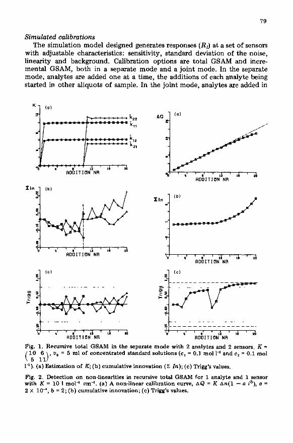
Fig. 1. Recursive total GSAM in the separate mode with 2 analytes and 2 sensors. K =

e f-1)* “O = 5 ml of concentrated standard solutions (c, = 0.1 mol 1-l and c, = 0.1 mol

1-l). (a) Estimation of K; (b) cumulative innovation (Z In); (c) Trigg’s values.

Fig. 2. Detection on non-linearities in recursive total GSAM for 1 analyte and 1 sensor with K = 10 1 mol-’ cm-‘. (a) A non-linear calibration curve, AQ = K An(1 - a ib), a = 2 x 10e4, b = 2; (b) cumulative innovation; (c) Trigg’s values.

80

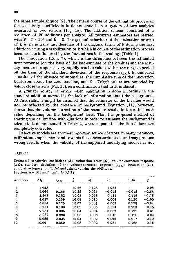
the same sample aliquot [2] . The general course of the estimation process of the sensitivity coefficients is demonstrated on a system of two analytes measured at two sensors (Fig. la). The addition scheme consisted of a sequence of 20 additions per analyte. All recursive estimators are started with P=I* lo6 and k = 0. The general behaviour of the estimation process of k is an initially fast decrease of the diagonal terms of P during the first additions causing a stabilization of k which in course of the estimation process becomes less influenced by the fluctuations in the readings (Table 1).

The innovation (Eqn. 7), which is the difference between the estimated next response (on the basis of the last estimate of the k value) and the actu- ally measured response, very rapidly reaches values within the range expected on the basis of the standard deviation of the response (sao). In this ideal situation of the absence of anomalies, the cumulative sum of the innovation fluctuates about the zero baseline, and the Trigg’s values are bounded by values close to zero (Fig. lc), as a confirmation that drift is absent.

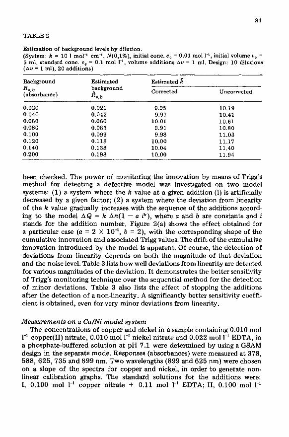
A primary source of errors when calibration is done according to the standard addition method is the lack of information about the background. At first sight, it might be assumed that the estimates of the k values would not be affected by the presence of background. Equation (ll), however, shows that the volume correction of the response results in the estimated k value depending on the background level. That the proposed method of starting the calibration with dilutions in order to estimate the background is adequate is demonstrated in Table 2, where apparent calibration failures are completely corrected.

Defective models are another important source of errors. In many instances, calibration graphs may bend towards the concentration axis, and may produce wrong results when the validity of the supposed underlying model has not

TABLE 1

Estimated sensitivity coefficient (&), estimation error (si), volume-corrected response (AQ), standard deviation of the volume-corrected response (SA Q), innovation (In), cumulative innovation (X In) and gain (g) during the additions. [System: k = 10 1 mol-’ cm-‘, N(O,l%)]

Addition AQ SAG! R G In 1: In g

1 1.028 - 10.26 0.126 -1.023 - -9.98

2 2.069 0.165 10.32 0.036 -0.018 -0.018 -3.58 3 2.962 0.152 10.08 0.016 0.134 0.116 -1.78 4 4.029 0.159 10.08 0.010 0.004 0.120 -1.00 5 5.034 0.175 10.07 0.007 0.005 0.125 -0.64 6 5.931 0.186 10.02 0.005 0.114 0.239 -0.45 7 7.084 0.205 10.04 0.004 -0.067 0.172 -0.31 8 8.082 0.223 10.06 0.003 -0.046 0.126 -0.24 9 8.959 0.238 10.04 0.002 0.090 0.217 -0.19

10 10.09 0.259 10.05 0.002 -0.051 0.165 -0.15

81

TABLE 2

Estimation of background levels by dilution. (System: k = 10 1 mol-’ cm-‘, N(O,l%), initial cont. c, = 0.01 mol l-l, initial volume LJ, = 5 ml, standard cont. c, = 0.1 mol l-‘, volume additions Au = 1 ml. Design: 10 dilutions (Au = 1 ml), 20 additions)

Background R o,b (absorbance)

Estimated background

k,b

Estimated 6

Corrected Uncorrected

0.020 0.021 9.95 10.19 0.040 0.042 9.97 10.41 0.060 0.060 10.01 10.61 0.080 0.083 9.91 10.80 0.100 0.099 9.98 11.03 0.120 0.118 10.00 11.17 0.140 0.138 10.04 11.40 0.200 0.198 10.00 11.94

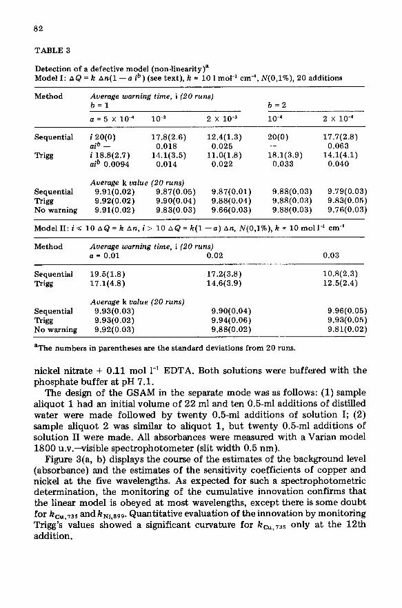
been checked. The power of monitoring the innovation by means of Trigg’s method for detecting a defective model was investigated on two model systems: (1) a system where the k value at a given addition (i) is artificially decreased by a given factor; (2) a system where the deviation from linearity of the k value gradually increases with the sequence of the additions accord- ing to the model A& = k An(1 - a ib), where a and b are constants and i stands for the addition number. Figure 2(a) shows the effect obtained for a particular case (a = 2 X 104, b = 2), with the corresponding shape of the cumulative innovation and associated Trigg values. The drift of the cumulative innovation introduced by the model is apparent. Of course, the detection of deviations from linearity depends on both the magnitude of that deviation and the noise level. Table 3 lists how well deviations from linearity are detected for various magnitudes of the deviation. It demonstrates the better sensitivity of Trigg’s monitoring technique over the sequential method for the detection of minor deviations. Table 3 also lists the effect of stopping the additions after the detection of a non-linearity. A significantly better sensitivity coeffi- cient is obtained, even for very minor deviations from linearity.

Measurements on a Cu/Ni model system The concentrations of copper and nickel in a sample containing 0.010 mol

1-l copper(I1) nitrate, 0.010 molI1 nickel nitrate and 0.022 mol 1-l EDTA, in a phosphate-buffered solution at pH 7.1 were determined by using a GSAM design in the separate mode. Responses (absorbances) were measured at 378, 588, 625,735 and 899 nm. Two wavelengths (899 and 625 nm) were chosen on a slope of the spectra for copper and nickel, in order to generate non- linear calibration graphs. The standard solutions for the additions were: I, 0.100 mol 1-l copper nitrate + 0.11 mol 1-l EDTA; II, 0.100 mol 1-l

82

TABLE 3

Detection of a defective model (non-linearity)a Model I: AQ = k An(1 --a ib) (see text), k = 10 1 mol-’ cm-‘, N(O,l%), 20 additions

Method Average warning time, i (20 runs) b=l

a=5 X lo+ 1o-3 2 x 1o-3

b=2

lOA 2 x 1o-4

Sequential

Trigg

i 20(O) 17.8(2.6) 12.4(1.3) 20(O) 17.7(2.8) sib - 0.018 0.025 - 0.063 i 18.8(2.7) ai”

14.1(3.5) ll.O(l.8) 18.1(3.9) 14.1(4.1) 0.0094 0.014 0.022 0.033 0.040

Average k value (20 runs) Sequential 9.91(0.02) 9.87(0.05) 9.87(0.01) g.BB(O.03) 9.79(0.03) Trigg 9.92(0.02) 9.90(0.04) g.BB(O.04) g.BB(O.03) 9.83(0.05) No warning 9.91(0.02) 9.83(0.03) 9.66(0.03) g.BB(O.03) 9.76(0.03)

Model II: i G 10 AQ = k An, i > 10 AQ = k(1 -a) An, N(O,l%), k = 10 mot 1-l cm-’

Method Average warning time, i (20 runs) a = 0.01 0.02 0.03

Sequential 19.5( 1.8) 17.2(3.8) 10.8(2.3) Trigg 17.1(4.8) 14.6(3.9) 12.5(2.4)

Average k value (20 runs) Sequential 9.93(0.03) 9.90(0.04) 9.96(0.05) Trigg 9.93(0.02) 9.94(0.06) 9.93(0.05) No warning 9.92(0.03) g.BB(O.02) g.Bl(O.02)

=The numbers in parentheses are the standard deviations from 20 runs.

nickel nitrate + 0.11 mol 1-l EDTA. Both solutions were buffered with the phosphate buffer at pH 7.1.

The design of the GSAM in the separate mode was as follows: (1) sample aliquot 1 had an initial volume of 22 ml and ten 0.5-ml additions of distilled water were made followed by twenty 0.5~ml additions of solution I; (2) sample ahquot 2 was similar to aliquot 1, but twenty 0.5-ml additions of solution II were made. All absorbances were measured with a Varian model 1800 u.v.-visible spectrophotometer (slit width 0.5 nm).

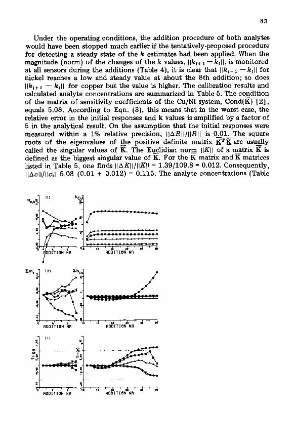
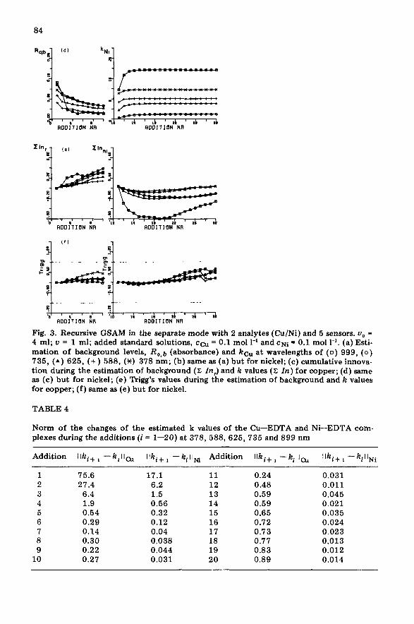
Figure 3(a, b) displays the course of the estimates of the background level (absorbance) and the estimates of the sensitivity coefficients of copper and nickel at the five wavelengths. As expected for such a spectrophotometric determination, the monitoring of the cumulative innovation confirms that the linear model is obeyed at most wavelengths, except there is some doubt for kcU,,35 and kNi.899. Quantitative evaluation of the innovation by monitoring Trigg’s values showed a significant curvature for km,,35 only at the 12th addition.

83

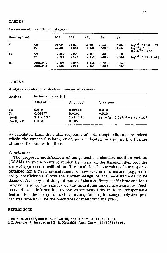
Under the operating conditions, the addition procedure of both analytes would have been stopped much earlier if the tentatively-proposed procedure for detecting a steady state of the k estimates had been applied. When the magnitude (norm) of the changes of the k values, Ilki+ I - k,ll, is monitored at all sensors during the additions (Table 4), it is clear that I Iki+ 1 -kill for nickel reaches a low and steady value at about the 8th addition; so does Ilki+ 1 - kil I for copper but the value is higher. The calibration results and calculated analyte concentrations are summarized in Table 5. The coEdition of the matrix of sensitivity coefficients of the Cu/Ni system, Cond(K) [ 21, equals 5.08. According to Eqn. (3), this means that in the worst case, the relative error in the initial responses and k values is amplified by a factor of 5 in the analytical result. On the assumption that the initial responses were measured within a 1% relative precision, IlARII/IIRII is 0.01. The square roots of the eigenvalues of @e positive definite matrix KTK are usually called the singular values of K. The Euclidian norm IlKI of a m_atrix g is defined as the biggest singular value of K. For the K matrix and K matrices listed in Table 5,-&e finds llAKll/llKll = 1.39/109.8 = 0.012. Consequently, llAcll/llcll 5.08 to.01 + 0.012) = 0.115. The analyte concentrations (Table

RDLIITION NR

ALlDITI(IN NR

Fig. 3. Recursive GSAM in the separate mode with 2 analytes (Cu/Ni) and 5 sensors. U, = 4 ml; u = 1 ml; added standard solutions, ca = 0.1 mol 1-l and CNi = 0.1 mol 1-l. (a) Esti- mation of background levels, R,*b (absorbance) and kcu at wavelengths of (0) 999, (0) 735, (A) 625, (+) 588, (X) 378 nm; (b) same as (a) but for nickel; (c) cumulative innova- tion during the estimation of background (X In> and k values (2: Zn) for copper; (d) same as (c) but for nickel; (e) Trigg’s values during the estimation of background and k values for copper; (f) same as (e) but for nickel.

TABLE 4

Norm of the changes of the estimated k values of the Cu-EDTA and Ni--EDTA com- plexes during the additions (i = l-20) at 378,588, 625, 735 and 899 nm

Addition Ilki+ 1 -k,ll, Ilk i+ I -kiilN Addition Ilki+ 1 -k$~, Ilk i+ I -kitlNi

1 75.6 2 27.4 3 6.4 4 1.9 5 0.54 6 0.29 7 0.14 8 0.30 9 0.22

10 0.27

17.1 6.2 1.5 0.56 0.32 0.12 0.04 0.038 0.044 0.031

11 0.24 0.031 12 0.48 0.011 13 0.59 0.045 14 0.59 0.021 15 0.65 0.035 16 0.72 0.024 17 0.73 0.023 18 0.77 0.013 19 0.83 0.012 20 0.89 0.014

85

TABLE 5

Calibration of the Cu/Ni model system

Wavelength(h) 899 736 626 688 378

ii CU 31.99 88.86 42.98 19.59 5.356 (h )I'* =109.8= IlKI Ni 19.26 1.831 6.036 8.008 11.66 (A!\"' = 21.6

SK CU Ni

. /, ~--- Cond(&= 5.08

0.380 0.90 0.36 0.20 0.123 0.385 0.677 0.344 0.203 0.151 (h,)"'=1.39= llAKl(

% Aliquotl 0.495 0.948 0.458 0.258 0.149 Aliquot2 0.528 0.938 0.467 0.264 0.153

TABLE 6

Analyte concentrations calculated from initial responses

Analyte Estimated cont. [Z]

Aliquot 1 Aliquot 2 True cont.

cu 0.010 0.00852 0.010 Ni 0.00977 0.0101 0.010 IlAcll 2.3 x lo-’ 1.48 x 10-j llcll= (2 x 0.01’)“’ = 1.41 x lo-’ llAcll/llcll 0.016 0.105

6) calculated from the initial responses of both sample aliquots are indeed within the expected relative error, as is indicated by the I IAclI/IlclI values obtained for both estimations.

Conclusions The proposed modification of the generalized standard addition method

(GSAM) to give a recursive version by means of the Kalman filter provides a novel approach to calibration. The “real-time” conversion of the response obtained for a given measurement to new system information (e.g., sensi- tivity coefficients) allows the further design of the measurements to be decided. At every addition, estimates of the sensitivity coefficients and their precision and of the validity of the underlying model, are available. Feed- back of such information to the experimental design is an indispensable feature for the design of self-calibrating (and optimizing) analytical pro- cedures, which will be the nrecursors of intelligent analyzers.

REFERENCES

1 Bo E. H. Saxberg and B. R. Kowalski, Anal. Chem., 51 (1979) 1031. 2 C. Jochum, P. Jochum and B. R. Kowslski, Anal. Chem., 53 (1981) 8592.

3 H. N. J. Poulisse, Anal. Chim. Acta, 112 (1979) 361. 4 C. B. M. Didden and H. N. J. Poulisse, Anal. Lett., 13(All) (1980) 921. 5 H. N. J. Poulisse and P. Engelen, Anal. Lett., 13(A14) (1980) 1211. 6 P. F. Seelig and H. N. Blount, Anal. Chem., 51 (1979) 327. 7 G. A. Barnard, J. R. Stat. Sot., Part B, 21 (1959) 239. 8 D. L. Massart, A. Dijkstra and L. Kaufman, Evaluation and Optimization of Laboratory

Methods and Analytical Procedures, Elsevier, Amsterdam, 1978.