International Journal of Computer Applications (0975 – 8887)

Volume 15– No.8, February 2011

27

Speech Recognition by Wavelet Analysis

Nitin Trivedi

Asstt. Prof. Vidya College of Engg.

Meerut

Sachin Ahuja

Asstt. Prof. Vidya College of Engg.

Meerut

Dr. Vikesh Kumar Director

Vidya College of Engg. Meerut

Raman Chadha

Asstt. Prof. Vidya College of Engg.

Meerut

Saurabh Singh

Asstt. Prof. Vidya College of Engg.

Meerut

ABSTRACT

In an effort to provide a more efficient representation of the

speech signal, the application of the wavelet analysis is

considered. This research presents an effective and robust

method for extracting features for speech processing. Based

on the time‐frequency multi‐resolution property of wavelet

transform, the input speech signal is decomposed into various

frequency channels.

The major issues concerning the design of this Wavelet based

speech recognition system are choosing optimal wavelets for

speech signals, decomposition level in the DWT, selecting the

feature vectors from the wavelet coefficients. More

specifically automatic classification of various speech signals

using the DWT is described and compared using different

wavelets. Finally, wavelet based feature extraction system and

its performance on an isolated word recognition problem are

investigated. For the classification of the words, three layered

feed forward network is used.

General Terms

Dynamic Time Warping (DTW) Algorithm, Wavelet

Transform (WT).

Keywords Speech recognition, feature extraction, wavelet transform,

Discrete Wavelet Transform (DWT).

1. INTRODUCTION

Speech recognition is the process of automatically extracting

and determining linguistic information conveyed by a speech

signal using computers or electronic circuits. Automatic

speech recognition methods, investigated for many years have

been principally aimed at realizing transcription and human

computer interaction systems. The first technical paper to

appear on speech recognition has since then intensified the

researches in this field, and speech recognizers for

communicating with machines through speech have recently

been constructed, although they remain only of limited use.

Automatic speech recognition (ASR) features some of the

following advantages:

Speech input is easy to perform because it does not

require a specialized skill as does typing or pushbutton

operations.

Information can be input even when the user is moving

or doing other activities involving the hands, legs, eyes,

or ears.

Since a microphone or telephone can be used as an

input terminal, inputting information is economical with

remote inputting capable of being accomplished over

existing telephone networks and the Internet.

However, the task of ASR is difficult because:

Lot of redundancy is present in the speech signal that

makes discriminating between the classes difficult.

Presence of temporal and frequency variability such as

intra speaker variability in pronunciation of words and

phonemes as well as inter speaker variability e.g. the

effect of regional dialects.

Context dependent pronunciation of the phonemes

(co‐articulation).

Signal degradation due to additive and convolution noise

present in the background or in the channel

Signal distortion due to non‐ideal channel characteristic.

2. SPEECH RECOGNITION Most speech recognition systems can be classified

according to the following categories:

2.1 Speaker Dependent vs. Speaker

Independent A speaker‐dependent speech recognition system is one that is

trained to recognize the speech of only one speaker. Such

systems are custom built for just a single person, and are

hence not commercially viable. Conversely, a

speaker‐independent system is one that is independence is

hard to achieve, as speech recognition systems tend to become

attuned to the speakers they are trained on, resulting in error

rates that are higher than speaker dependent systems.

2.2 Isolated vs. Continuous In isolated speech, the speaker pauses momentarily between

every word, while in continuous speech the speaker speaks in

a continuous and possibly long stream, with little or no breaks

in between. Isolated speech recognition systems are easy to

build, as it is trivial to determine where one word ends and

another starts, and each word tends to be more cleanly and

clearly spoken. Words spoken in continuous speech on the

other hand are subjected to the co-articulation effect, in which

the pronunciation of a word is modified by the words

surrounding it. This makes training a speech system difficult,

as there may be many inconsistent pronunciations for the

same word.

2.3 Keyword‐based vs. Sub‐word unit based A speech recognition system can be trained to recognized

whole words, like dog or cat. This is useful in applications

International Journal of Computer Applications (0975 – 8887)

Volume 15– No.8, February 2011

28

like voice‐command‐systems, in which the system need only

recognize a small set of words. This approach, while simple,

is unfortunately not scalable [8]. As the dictionary of

recognized words grow, so too the complexity and execution

time of the recognizer. A more practical approach would be to

train the recognition system to recognize sub‐word units like

syllables or phonemes (phonemes are the smallest atomic

speech sound, like the „w‟ and „iy‟ sounds in „we‟), and then

re‐construct the word based on which syllables or phonemes

are recognized.

For speech recognition, some of its characteristics (features)

in time/frequency or in some other domain must be known. So

a basic requirement of a speech recognition system will be to

extract a set of features for each of the basic units. A feature

can be defined as a minimal unit, which distinguishes

maximally close units. The feature vector extracted should

possess the following properties:

Vary widely from class to class.

Stable over a long period of time.

Can be easily computed from the input speech samples.

Should be small in dimension.

Should be insensitive to the irrelevant variation in the

speech.

Should not have correlation with other features.

3. WAVELET ANALYSIS

3.1 Introducing Wavelet The fundamental idea behind wavelets is to analyze according

to scale. The wavelet analysis procedure is to adopt a wavelet

prototype function called an analyzing wavelet or mother

wavelet. Any speech signal can then be represented by

translated and scaled versions of the mother wavelet. Wavelet analysis is capable of revealing aspects of data that

other speech signal analysis technique such the extracted

features are then passed to a classifier for the recognition of

isolated words.

3.2 Statement of the Problem In this research, the problem of recognizing a small set of

prescribed vocabulary words spoken is investigated. It

describes a new method for speaker‐independent word

recognition using wavelet transform (WT) features. While

much research has been performed in cepstral analysis, very

little has been performed in wavelet domain for speech

analysis. In principle, this research is a modification of the

previous methods which is applied for speech recognition.

The differences between the present word recognition method

and the previous method lie in the features selected for

analysis and in the length of the period for extracting the

wavelet features. The number of levels of wavelet

decomposition and the type of decomposition are different

from the previous methods applied for speech recognition.

Lastly, some of the wavelet features are proposed which are

new in speech recognition.

3.3 Examples of Wavelet The different families make trade‐offs between how

compactly the basis functions are localized in space and how

smooth they are. Within each family of wavelets (such as the

Daubechies family) are wavelet subclasses distinguished by

the number of filter coefficients and the level of iteration.

Wavelets are most often classified within a family by the

number of vanishing moments. This is an extra set of

mathematical relationships for the coefficients that must be

satisfied. The extent of compactness of signals depends on the

number of vanishing moments of the wavelet function used.

3.4 Daubechies‐N Wavelet family The Daubechies wavelet is one of the popular wavelets and

has been used for speech recognition [1]. It is named after its

inventor, the mathematician Ingrid Daubechies. These

wavelets have no explicit expression except for db1, which is

the Haar wavelet. The Daubechies wavelets properties:

The support length of the wavelet function Ψ and the

scaling function Φ is 2N‐1. The number of vanishing

moments of Ψ is N.

Most dbN are not symmetrical.

The regularity increases with the order. When N

becomes very large, Ψ and Φ belong to CμN

where μ is

approximately equal to 0.2.

Daubechies‐8 wavelet is used for decomposition of speech

signal as it needs minimum support size for the given number

of vanishing points [4].

4. THE DISCRETE WAVELET

TRANSFORM The Discrete Wavelet Transform (DWT) involves choosing

scales and positions based on powers of two ‐ so called dyadic

scales and positions [5]. The mother wavelet is rescaled or dilated, by powers of two

and translated by integers.

Specifically, a function f(t) Є L2

(R) (defines space of square

integrable functions) can be represented as f(t) = ΣJ=1 – L

Σ K= α

to –α d(j,k) ψ(2

‐j

t‐k) +Σ K= α to –α

a(L,k) φ(2‐L

t‐k)

The function ψ(t) is known as the mother wavelet, while φ(t)

is known as the scaling function. The set of functions {√2‐L

φ(2‐L

t‐k), √2‐j

ψ(2‐j

t‐k) |j<=L,j,k,LЄZ }, where Z is the set of

integers, is an orthonormal basis for L2

(R).

The numbers a(L, k) are known as the approximation

coefficients at scale L, while d(j,k) are known as the detail

coefficients at scale j. The approximation and detail

coefficients can be expressed as:

a(L,k) = 1/√2 ∫α

–α

f(t) φ(2‐L

t‐k)dt

d(j,k) = 1/√2 ∫α

–α

f(t) ψ(2‐j

t‐k)dt

To provide some understanding of the above coefficients

consider a projection fl(t) of the function f(t) that provides the

best approximation (in the sense of minimum error energy) to

f(t) at a scale l. This projection can be constructed from the

coefficients a(L,k), using the equation

fl(t) = Σ

K= α to –α a(l,k) φ(2

‐l

t‐k)

As the scale l decreases, the approximation becomes finer,

converging to f(t) as l→0. The difference between the

approximation at scale l + 1 and that at l, fl+1

(t) ‐ fl(t), is

completely described by the coefficients d(j, k) using the

equation

fl+1

(t) ‐ fl(t) = Σ

K= α to –α d(l,k) ψ(2

‐l

t‐k)

Using these relations, given a(L, k) and {d(j, k) | j <= L}, it is

clear that we can build the approximation at any scale. Hence,

the wavelet transform breaks the signal up into a coarse

approximation fL(t) (given a(L, k)) and a number of layers of

detail {fj+1

(t)‐fj(t)| j< L} (given by {d(j, k) | j ≤ L}). As each

layer of detail is added, the approximation at the next finer

scale is achieved.

International Journal of Computer Applications (0975 – 8887)

Volume 15– No.8, February 2011

29

4.1 The Fast Wavelet Transform Algorithm The Discrete Wavelet Transform (DWT) coefficients can be

computed by using Mallat‟s [2] Fast Wavelet Transform

algorithm. This algorithm is sometimes referred to as the

two‐channel sub‐band coder and involves filtering the input

signal based on the wavelet function used. Consider the

following equations:

φ(t) = Σk

c(k) φ(2t‐k)

ψ(t) = ΣK

(‐1)k

c(1‐k) φ(2t‐k)

ΣK

ck

ck‐2m

= 2δ0,m

The first equation is known as the twin‐scale relation (or

the dilation equation) and defines the scaling function φ. The

next equation expresses the wavelet ψ in terms of the scaling

function φ. The third equation is the condition required for the

wavelet to be orthogonal to the scaling function.

The coefficients c(k) or {c0, ….., c

2N‐1} in the above equations

represent the impulse response coefficients for a low pass

filter of length 2N, with a sum of 1 and a norm of 1/√2.

Starting with a discrete input signal vector s, the first stage of

the FWT algorithm decomposes the signal into two sets of

coefficients. These are the approximation coefficients cA1

(low frequency information) and the detail coefficients cD1

(high frequency information), as shown in the figure below.

Fig 1: Filtering Analysis of DWT

4.2 Multilevel Decomposition The decomposition process can be iterated, with successive

approximations being decomposed in turn, so that one signal

is broken down into many lower resolution components. This

is called the wavelet decomposition tree [6].

Fig 2: Decomposition of DWT Coefficient

The wavelet decomposition of the signal„s‟ analyzed at level

„j‟ has the following structure [cAj, cD

j,..., cD

1].

Looking at a signals wavelet decomposition tree can reveal

valuable information. The diagram below shows the wavelet

decomposition to level 3 of a sample signal S.

Fig 3: Level 3 Decomposition of Sample Signal S

Since the analysis process is iterative, in theory it can be

continued indefinitely. In reality, the decomposition can only

proceed until the vector consists of a single sample. Normally,

however there is little or no advantage gained in decomposing

a signal beyond a certain level. The selection of the optimal

decomposition level in the hierarchy depends on the nature of

the signal being analyzed or some other suitable criterion,

such as the low‐pass filter cut‐off.

4.3 Signal Reconstruction The original signal can be reconstructed or synthesized using

the inverse discrete wavelet transform (IDWT).

The synthesis starts with the approximation and detail

coefficients cAj

and cDj, and then reconstructs cA

j‐1 by up

sampling and filtering with the reconstruction filters.

The reconstruction filters are designed in such a way to cancel

out the effects of aliasing introduced in the wavelet

decomposition phase [8]. The reconstruction filters (Lo_R and

Hi_R) together with the low and high pass decomposition

filters, forms a system known as quadrature mirror filters

(QMF).

Fig 4: Signal Reconstruction

5. METHODOLOGY The different steps involved in the proposed method are

preprocessing, frame blocking & windowing, wavelet feature

extraction and the word recognition module which are given

as follows:

Fig 5: Design overview of speech recognition process

5.1 Preprocessing

The objective in the preprocessing is to modify the speech

signal, so that it will be more suitable for the feature

extraction analysis. The preprocessing consists of de‐noising,

pre‐emphasis and voice activation detection.

International Journal of Computer Applications (0975 – 8887)

Volume 15– No.8, February 2011

30

Fig 6: Preprocessing of Speech Signal

Automatic speech recognition involves a number of

disciplines such as physiology, acoustics, signal processing,

pattern recognition, and linguistics. The difficulty of

automatic speech recognition is coming from many aspects of

these areas. A survey of robustness issues in automatic speech

recognition may be found in [3].

5.2 Voice Activation Detection (VAD) The problem of locating the endpoints of an utterance in a

speech signal is a major problem for the speech recognizer.

Inaccurate endpoint detection will decrease the performance

of the speech recognizer. The problem of detecting endpoints

seems to be relatively trivial, but it has been found to be very

difficult in practice. Some commonly used measurements for

finding speech are short‐term energy estimate Es1

, or

short‐term power estimate Ps1

, and short term zero crossing

rate Zs1

. For the speech signal s1(n) these measures are

calculated as follows:

Es1

(m) = Σn=m−L+1 to m

s1

2

(n)

Ps1

(m) = 1/L Σn=m−L+1 to m

s1

2

(n)

Zs1

(m) = 1/L Σn=m−L+1 to m

|sgn(s1(n)) -

. sgn(s1(n‐1))|/2

Where sgn(s1(n)) = +1 if s

1(n)> 0

sgn(s1(n))= ‐1 if s

1(n)≤ 0

These measures will need some triggers for making decision

about where the utterances begin and end. To create a trigger,

one should need some information about the background

noise. This is done by assuming that the first 10 blocks are

background noise. The trigger for this function can be

described as:

tW

= μW

+ αδW

The μW

is the mean and δW

is the variance calculated for the

first 10 blocks. The α term is a constant that have to be fine

tuned according to the characteristics of the signal which is

given as α = 0.2 δW

−0.8

The voice activation detection function, VAD(m), can now be

found as:

VAD(m) = 1, W

s1(m) ≥ t

W = 0, W

s1(m)< t

W

Where Ws1

(m) = Ps1

(m) ∙ (1 − Z s1

(m)) ∙ Sc

Sc= 1000

5.3 Frame Blocking and Windowing Before Frame blocking and Windowing, the duration of the

word must be equal for all the utterances in order to divide the

signal into equal number of frames. This can be achieved by

using Dynamic Time Warping (DTW) explained below:

Dynamic Time Warping Even if the same speaker utters the same word, the

duration changes every time with nonlinear expansion and

contraction. Therefore, Dynamic Time Warping (DTW) is

essential at the word recognition stage. The DTW process

nonlinearly expands or contracts the time axis to match the

same word.

The DTW algorithm is given as follow:

Let A & B be the sequence vectors which are to be compared, A = a

1, a

2, a

3, ………., a

I and B = b

1, b

2, b

3,……., b

J

The warping function indicating the correspondence between

the time axes of A and B sequences can be represented by a

sequence of lattice points on the plane, c = (i,j), as

F = c1, c

2, c

3… c

k, c

k= (i

k,j

k)

When the spectral distance between two feature vectors ai and

bj is presented by d(c) = d(i,j), the sum of the distances from

beginning to end of the sequences along F can be represented

by D(F) = Σ

k=1 to K d(c

k) w

k / Σ

k=1 to K w

k

The smaller the value of D(F), the better the match between A

and B. wk

is a positive weighting function related to F.

Fig 7: Dynamic Time warping between two time sequences

For minimizing the concerning F consider the following

conditions.

1. Monotony and continuity condition

0 ≤ ik ‐ i

k‐1 ≤ 1, 0 ≤ j

k ‐ j

k‐1 ≤ 1

2. Boundary condition i1

= j1 = 1, i

k = I, j

K = J

3. Adjustment window condition

|ik ‐ i

k| ≤ r, r=constant if w

k=(i

k ‐ i

k‐1)

+ (jk ‐ j

k‐1) then

Σk=1 to K

wk

= I+J. Also

D(F) = 1/(I+J) Σk=1 to K

d(ck) w

k.

Since, the objective function to be minimized becomes

additive, minimization can be efficiently done as follows:

g(Ck) = g(i,j) = min c

k‐1 [g(c

k‐1)+d(c

k)w

k]

Which can be rewritten as

g(i,j) = min { g(1,j‐1)+ d(i,j), g(1‐i,j‐1)+

2d(i,j), g(1‐i,j)+ d(i,j)}

g(1,1) = 2d(1,1)

Once Dynamic Time Warping is done, the next step is to

divide the speech signal into different frames and then

applying hamming windowing for each frame which can be

done as follows:

Fig 8: Frame blocking & windowing

International Journal of Computer Applications (0975 – 8887)

Volume 15– No.8, February 2011

31

For each utterances of the word, a window duration of

Tw=32ms is used for processing at later stages. A frame is

formed from the windowed data with typical frame duration

(Tf) of about 20ms. Since the frame duration is shorter than

window duration there is an overlap of data and the

percentage overlap is given as:

% Overlap = ((Tw‐T

f)*100)/T

w

Each frame is 32ms samples long, with adjacent frames being

separated by 20ms samples as shown in the following

diagram.

Fig 9: Frame blocking of a sequence

The Hamming window to each frame is applied in order to

reduce signal discontinuity at either end of the block. It is

calculated as follows:

w(k) = 0.54 – 0.46cos(2Πk/K‐1)

6. Result The results obtained after each stage are given as follows:

1. In the preprocessing, the first step is the Voice Activation

Detection (VAD) and segmenting the speech signal

accordingly. The VADs obtained for the speech sample of

the words ‘option’ and ‘subhash’ are given below:

Fig 10: VADs for The Speech Samples

2. The second step of the preprocessing is De‐noising. The

utterances of the speech sample „file‟ with the background

noise and after de‐noising of the sample are given below:

Fig 11: Denoising of the Speech Sample

3. Once the preprocessing is done, the next step is framing

and blocking, the frames obtained for the speech sample

‘close’ of window size 32ms with 10ms overlapping is

given below:

Fig 12: Framing of Speech Sample ‘file’

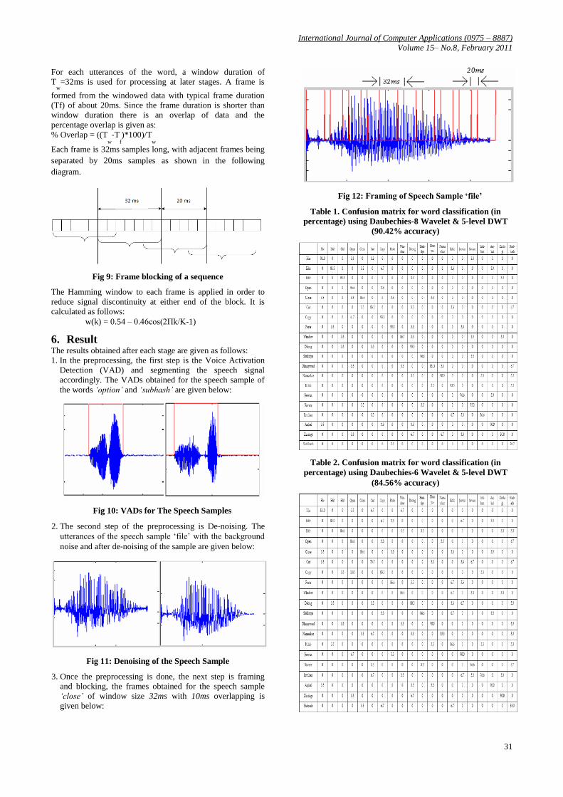
Table 1. Confusion matrix for word classification (in

percentage) using Daubechies-8 Wavelet & 5-level DWT

(90.42% accuracy)

Table 2. Confusion matrix for word classification (in

percentage) using Daubechies‐6 Wavelet & 5‐level DWT

(84.56% accuracy)

International Journal of Computer Applications (0975 – 8887)

Volume 15– No.8, February 2011

32

7. CONCLUSION The features obtained by using the wavelet transform shows

higher recognition rates if the features are extracted properly.

Wavelets proved to have both strengths and weaknesses for

speech feature identification. In general, wavelets are able to

distinguish between different properties high frequency low

amplitude spectral components and low frequency large

amplitude spectral components Also, neural network classifier

improves the recognition performance significantly. The

result shows that the wavelet transform can be effectively

used for the extraction of features for speaker independent

word recognition. Higher recognition performance can be

achieved by using more complex classification techniques.

8. FUTURE WORK The exact details of feature calculation for MFCC have been

explored extensively in the literature. On the other hand,

wavelet based features have appeared relatively recently.

Further improvements in classification accuracy can be

expected with more careful experimentation with the exact

details of the parameters and for other wavelet families.

Another interesting direction is combining features from

different analysis techniques to improve classification

accuracy.

9. REFERENCES [1] B.T. Tan, M. Fu, A. Spray, P. Dermody, “The use of

wavelet transform for phoneme recognition,”

Proceedings of the 4th International Conference of

Spoken Language Processing Philadelphia, Vol. 4, USA,

October 1996, pp.2431-2434.

[2] S. G. Mallat, “A theory for multiresolution signal

decomposition: the wavelet representation,” IEEE

transactions on Pattern Analysis Machine Intelligence,

Vol. 11 1989, pp.674-693.

[3] Oliver Siohan and Chin-Hui Lee “Iterative Noise and

Channel Estimation under the Stochastic Matching

Algorithm Framework” IEEE Signal Processing,

Processing Letters, Vol. 4, No. 11, Nov 1997.

[4] M. Misiti, Y. Misiti, G. Oppenheim and J. Poggi, Matlab

Wavelet Tool Box, The Math Works Inc.,2000 Page: 795.

[5] George Tzanetakis, Georg Essl, Perry Cook, “Audio

Analysis using the Discrete Wavelet Transform”

Organized sound, Vol. 4(3), 2000.

[6] L. Barbier, G. Chollet, “Robust speech parameters

extraction for word recognition in noise using neural

networks,” IEEE International Conference on Acoustics,

Speech, and Signal Processing, Pages: 145-148, May

1991.

[7] X. Huang, “Speaker normalization for speech

recognition”, IEEE International Conference on

Acoustics, Speech, and Signal Processing, 1:465-468,

March 1992.

[8] S. Tamura, A Waibel, “Noise reduction using

connectionist models.” IEEE International Conference

on Acoustics, Speech, and Signal Processing, 1:553-556,

April 1988.

[9] S. Young, “A review of large vocabulary continues-

speech recognition,” Proc. IEEE Sig. Processing. Mag.

(September) (1996) 45-57.

[10] N. Desmukh, A. Ganapathiraju, J. Picone, “Hierarchical

search for large vocabulary conversational speech

recognition – working toward a solution to the decoding

problem,” IEEE Sig, Process Mag. (September) (1999)

84-107.