Isolated Tamil Digits Speech Recognition using Vector ... - IJERT

Isolated Tamil Digits Speech Recognition using Vector Quantization

S.Karpagavalli*

Assistant Professor

PSGR Krishnammal College for Women

[email protected]

Coimbatore

K.Usha Rani, R.Deepika, P.Kokila

Mphil Research Scholar

PSGR Krishnammal College for Women

Abstract

Automatic recognition of spoken digits is one of

the challenging tasks in the field of ASR. Spoken

digits recognition process is needed in many

applications that need numbers as input like

telephone dialing using speech, addresses, airline

reservation, and automatic directory to retrieve or

send information, hands and eyes free applications.

ASR has attained a maturity level in English

Language. In Indian Languages, very few research

work carried out and many more levels to be

reached. Building a speech recognizer for the

Indian language like Tamil is a challenging task

due to the unique inherent features of the language.

In this work, small vocabulary, isolated, speaker

independent, Tamil digits recognizer has been

designed and the performance of the recognizer is

analyzed. The various task involved in this work

are speech corpus preparation, feature extraction,

code book generation for each word in the

vocabulary, and testing the recognizer. Codebook

for each word in the vocabulary created using

Linde-Buzo-Gray (LBG) vector quantization

algorithm. The performance of the speech

recognizer for each digit is analyzed and evaluated

using Word Error Rate and Word Recognition Rate

1. Introduction Speech is the most natural form of human

communication and speech processing has been

one of the most exciting areas of the signal

processing. Speech Recognition is the process of

converting a speech signal to a sequence of words,

by means of an algorithm implemented as a

computer program.

The functionality of automatic speech

recognition system can be described as an

extraction of a number of speech parameters from

the acoustic speech signal for each word. The

speech parameters describe the word by their

variation over time and together they build up a

pattern that characterizes the word.

In a training phase the operator will read all

the words of the vocabulary of the current

application. The word patterns are stored and later

when a word is to be recognized its pattern is

compared to the stored patterns and the word that

gives the best match is selected.

1.1 Mathematical representation

Fundamentally, the problem of speech

recognition can be stated as follows. When given

with acoustic observation O = o1o2…ot, the goal is

to find out the corresponding word sequence W =

w1w2…wn that has the maximum posterior

probability P (W|O) can be written as

. . . . . . . (1)

Equation 1 can be expressed using Bayes rule as

. . . . . . (2)

Since the P (O) is the same for each candidate

sentence W, thus equation 2 can be reduced as

. . . . . . . (3)

Where P (W), the prior probability of word W

uttered is called the language model and P (O|W),

the observation likelihood of acoustic observation

O when word W is uttered is called the acoustic

model [1].

1.2 Issues in Speech Recognition

There are number of issues that need to be

addressed in order to define the operating range of

each speech recognizing systems that is built. Some

of them are, speech unit like word, syllable,

International Journal of Engineering Research & Technology (IJERT)

Vol. 1 Issue 4, June - 2012

ISSN: 2278-0181

1www.ijert.org

phoneme or phones used for recognition,

vocabulary size like small, medium and large, task

syntax like simple to complex task using N-gram

language models, task perplexity, speaking mode

like isolated, connected, continuous, spontaneous,

speaker mode like speaker trained, adaptive,

speaker independent, dependent, speaking

environment as quiet room, noisy places,

transducers may be high quality microphone,

telephones, cell phones, array microphones, and

also transmission channel. These issues are

discussed in detail below.

Speech unit for recognition: Ranging from words

down to syllables and finally to phonemes or even

phones. Early system investigated all these types of

unit with the goal of understanding their robustness

to context, speakers and speaking environments.

Vocabulary size: Ranging from small (order of 2-

100) words medium (order of 100-1000) words and

large (anything above 1000 words up to unlimited

vocabularies). Early system tackled primary small-

vocabulary recognition problem; modern speech

recognizer are all large-vocabulary system.

Task syntax: Ranging from simple task with

almost no syntax (every words in the vocabulary

can follow every other words) to highly complex

tasks where the words follow a statistical n-gram

language model.

Task perplexity: Ranging from low values (for

simple task) to values on the order of 100 for

complex task.

Speaking mode: Ranging from isolated words (or

short phrases), to connected word systems (e.g.,

sequence of digit that form identification codes or

telephone numbers), to continuous speech

(including both read passages and spontaneous

conversational speech).

Speaker mode: Ranging from speaker-trained

systems (works only on individual speakers who

trained the system) to speaker-adaptive systems

(works only after a period of adaptation to the

individual speaker‟s voice) to speaker-independent

systems that can be used by anyone without any

additional training. Most modern ASR (Automatic

Speech Recognition) systems or speaker

independent and are utilized in a range of

telecommunication application. However, for

dictation purpose, most systems are still largely

speaker dependent and adapt over time to each

individual speaker.

Speaking situation: Ranging from human-to-

machine dialogues to human-to-human dialogues

(e.g., as might be needed for language translation

system).

Speaking environment: Ranging from a quite

room to noisy place (e.g., offices, airline terminals)

and even outdoors (e.g., via the use of cell phones).

Transducers: Ranging from high- quality

microphones to telephones (wireline) to cellphones

(mobile) to array microphones (which track the

speaker location electronically).

Transmission channel: Ranging from simple

telephone channels, with -law speech coders in

the transmission path for wireline channels, to

wireless channels with fading and with a

sophisticated voice coder in the path.

1.3 Types of Speech Recognition

Speech recognition systems can be separated in

several different classes by describing what types

of utterances they have the ability to recognize [4].

These classes are classified as the following:

Isolated Words: Isolated word recognizers usually

require each utterance to have quiet (lack of an

audio signal) on both sides of the sample window.

It accepts single words or single utterance at a time.

These systems have "Listen/Not-Listen" states,

where they require the speaker to wait between

utterances (usually doing processing during the

pauses). Isolated Utterance might be a better name

for this class.

Connected Words: Connected word systems (or

more correctly 'connected utterances') are similar to

isolated words, but allows separate utterances to

'run-together' with a minimal pause between them.

Continuous Speech: Continuous speech

recognizers allow users to speak almost naturally,

while the continuous speech capabilities are some

of the most difficult to create because they utilize

special methods to determine utterance boundaries.

Spontaneous speech: At a basic level, it can be

thought of as speech that is natural sounding and

not rehearsed. An ASR system with spontaneous

speech ability should be able to handle a variety of

natural speech features such as words being run

together, "ums" and "ahs", and even slight stutters.

2. Speech Recognition Architecture

Speech recognition architecture is shown in

Figure 1 and its working principle is described

below.



ISSN: 2278-0181

2www.ijert.org

The input audio waveform from a microphone is

converted into a sequence of fixed-size acoustic

vectors in a process called feature extraction. The

decoder then attempts to find the sequence of

words that is most likely to generate. The

likelihood is defined as an acoustic model P (O|W)

and the prior P (W) is determined by a language

model. The acoustic model is not normalized and

the language model is often scaled by empirically

determined constant.

.

Figure 1.Speech Recognition Architecture

The parameters of these phone models are

estimated from training data consisting of speech

waveforms. The decoder operates by searching

through all possible word sequences thereby

keeping the search tractable [3].

Sampling: In speech recognition, Common

sampling rates are 8 KHz to 16 KHz, to accurately

measure a wave it is necessary to have at least two

samples in each cycle: one measuring the positive

part of the wave and one measuring the negative

part. More than two samples per cycle increases the

amplitude accuracy, but less than two samples will

cause the frequency of the wave to be completely

missed. For other applications commonly 16 KHz

sampling rate is used. Most information in human

speech is in frequencies below 10 KHz; thus a 20

KHz sampling rate would be necessary for

complete accuracy. But the switching network

filters telephone speech and only frequencies less

than 4 KHz are transmitted by telephones. Thus an

8 KHz sampling rate is sufficient for telephone/

mobile speech corpus [1].

Pre-Emphasis: The spectrum for voiced segments

has more energy at lower frequencies than higher

frequencies. Pre-emphasis is boosting the energy in

the high frequencies. Boosting high-frequency

energy gives more information to Acoustic Model

and improves the recognition performance. Pre-

emphasis of a speech signal at higher frequencies is

a processing step evolved in various speech

processing applications. Pre-emphasis of a speech

signal is achieved by the first order differencing of

a speech signal. Before pre-emphasis is original

wave is shown in Figure 2. Cepstral coefficients

derived through linear prediction analysis are used

as recognition parameters.

Figure 2.Original Wave

Figure 3.After pre-emphasis

The usual form for the pre-emphasis filter is a

high-pass FIR filter with the single zero near the

origin. This tends to whiten the speech spectrum as

well as emphasizing those frequencies to which the

human auditory system is most sensitive. However,

this is really only appropriate up to 3 to 4 kHz.

Above that range, the sensitivity of human hearing

falls off, and there is relatively little linguistic

information. Therefore, it is more appropriate to

use a second order pre-emphasis filter. This causes

the frequency response to roll off at higher

frequencies. This becomes very important in the

presence of noise.

Windowing and Framing: The time for which the

signal is considered for processing is called a

window and the data acquired in a window is called

as a frame. Typically features are extracted once

every 10ms, which is called as frame rate. The

window duration is typically 25ms. Thus two

consecutive frames have overlapping areas.

Original signal and Windowed signals are given

below.



ISSN: 2278-0181

3www.ijert.org

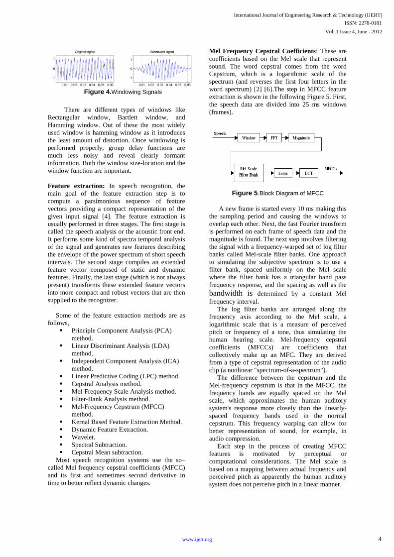
Figure 4.Windowing Signals

There are different types of windows like

Rectangular window, Bartlett window, and

Hamming window. Out of these the most widely

used window is hamming window as it introduces

the least amount of distortion. Once windowing is

performed properly, group delay functions are

much less noisy and reveal clearly formant

information. Both the window size-location and the

window function are important.

Feature extraction: In speech recognition, the

main goal of the feature extraction step is to

compute a parsimonious sequence of feature

vectors providing a compact representation of the

given input signal [4]. The feature extraction is

usually performed in three stages. The first stage is

called the speech analysis or the acoustic front end.

It performs some kind of spectra temporal analysis

of the signal and generates raw features describing

the envelope of the power spectrum of short speech

intervals. The second stage compiles an extended

feature vector composed of static and dynamic

features. Finally, the last stage (which is not always

present) transforms these extended feature vectors

into more compact and robust vectors that are then

supplied to the recognizer.

Some of the feature extraction methods are as

follows,

Principle Component Analysis (PCA)

method.

Linear Discriminant Analysis (LDA)

method.

Independent Component Analysis (ICA)

method.

Linear Predictive Coding (LPC) method.

Cepstral Analysis method.

Mel-Frequency Scale Analysis method.

Filter-Bank Analysis method.

Mel-Frequency Cepstrum (MFCC)

method.

Kernal Based Feature Extraction Method.

Dynamic Feature Extraction.

Wavelet.

Spectral Subtraction.

Cepstral Mean subtraction.

Most speech recognition systems use the so–

called Mel frequency cepstral coefficients (MFCC)

and its first and sometimes second derivative in

time to better reflect dynamic changes.

Mel Frequency Cepstral Coefficients: These are

coefficients based on the Mel scale that represent

sound. The word cepstral comes from the word

Cepstrum, which is a logarithmic scale of the

spectrum (and reverses the first four letters in the

word spectrum) [2] [6].The step in MFCC feature

extraction is shown in the following Figure 5. First,

the speech data are divided into 25 ms windows

(frames).

Figure 5.Block Diagram of MFCC

A new frame is started every 10 ms making this

the sampling period and causing the windows to

overlap each other. Next, the fast Fourier transform

is performed on each frame of speech data and the

magnitude is found. The next step involves filtering

the signal with a frequency-warped set of log filter

banks called Mel-scale filter banks. One approach

to simulating the subjective spectrum is to use a

filter bank, spaced uniformly on the Mel scale

where the filter bank has a triangular band pass

frequency response, and the spacing as well as the bandwidth is determined by a constant Mel

frequency interval.

The log filter banks are arranged along the

frequency axis according to the Mel scale, a

logarithmic scale that is a measure of perceived

pitch or frequency of a tone, thus simulating the

human hearing scale. Mel-frequency cepstral

coefficients (MFCCs) are coefficients that

collectively make up an MFC. They are derived

from a type of cepstral representation of the audio

clip (a nonlinear "spectrum-of-a-spectrum").

The difference between the cepstrum and the

Mel-frequency cepstrum is that in the MFCC, the

frequency bands are equally spaced on the Mel

scale, which approximates the human auditory

system's response more closely than the linearly-

spaced frequency bands used in the normal

cepstrum. This frequency warping can allow for

better representation of sound, for example, in

audio compression.

Each step in the process of creating MFCC

features is motivated by perceptual or

computational considerations. The Mel scale is

based on a mapping between actual frequency and

perceived pitch as apparently the human auditory

system does not perceive pitch in a linear manner.



ISSN: 2278-0181

4www.ijert.org

3. Vector quantization algorithm

Clustering is an important instrument in

engineering and other scientific disciplines. Its

applications cover several fields such as audio and

video, data compression, pattern recognition,

computer vision and medical image recognition.

Quantization converts a continuous-amplitude

signal to one of a set of discrete amplitude signals,

which is different from the original signal by the

quantization error. The independent quantization of

each signal parameter separately is termed scalar

quantization, while the joint quantization of a

vector is termed vector quantization (VQ). Vector

quantization can be thought of as a process of

redundancy removal that makes the effective use of

nonlinear dependency and dimensionality by

compression of speech spectral parameters.

Generally, the use of vector quantization results in

a lower distortion than the use of scalar

quantization at the same rate. The partitioning

approach known as Vector Quantization (VQ)

derives a set (codebook) of reference or prototype

vectors (codewords) from a data set. In this manner

each element of the data set is represented by only

one codeword.

Advantages of vector quantization representation

are,

Reduced storage for spectral analysis

information

Reduced computation for determining

similarity of spectral analysis vectors

Discrete representation of speech sounds

Disadvantages of vector quantization

representation are,

An inherent spectral distortion in

representing the actual analysis vector.

Since there is only a finite number of

codebook vectors, the process of choosing

the „best‟ representation of a given

spectral vector inherently is equivalent to

quantizing the vectors and leads, by

definition, to a certain level of

quantization error (QE). As the size of

codebook increases the size of the QE

decreases. However, with any finite code

book there will be always be some

nonzero level of quantization error.

The storage required for codebook vectors

is often nontrivial.

Elements of vector quantization

implementation: To build a VQ codebook and

implement a VQ analysis procedure [2] [7], the

following elements/procedure is needed.

Figure 6.Block Diagram of the basic VQ Training

and classification structure

1. A large set of spectral analysis vectors, x1,

x2, ……xL, which form a training set. The

training set used is used to create the

“optimal” set of codebook vector for

representing the spectral variability

observed in the training set. If we denote

the size of the VQ codebook as M=2B

vectors (we call this a B-bit codebook),

then we require L>>M so as to be able to

find the best set of M codebook vectors in

a robust manner. In practice, it has been

found that L should be least 10M in order

to train a VQ codebook that works

reasonably well.

2. A measure of similarity, or distance,

between a pair of spectral analysis vectors

so as to able to cluster the training set

vectors as well as to associate or classify

arbitrary spectral vectors into unique

codebook entries. The Spectral distance id

denoted as d (xi, xj), between two vectors

xi and xj and dij.

3. A centroid computation procedure. On the

basis of the partitioning that classifies the

L training set vector as well as into M

clusters, M codebook vectors are chosen

as the centroid of each of the M clusters.

4. A classification procedure for arbitrary

speech spectral analysis vectors that

chooses the codebook vector closest to the

input vector and uses the codebook index

as the resulting spectral representation.

This is often referred to as the nearest–

neighbor labeling or optimal encoding

procedure i.e. essentially a quantizer that

accepts, as input, speech spectral vector

and provides, as output, the codebook



ISSN: 2278-0181

5www.ijert.org

index of the codebook vector that best

matches the input.

The vector quantization training set

To properly train the VQ codebook, the

training set vectors should span anticipated range

of the following [2] [7]:

Talkers including ranges in age, accent,

gender, speaking rate, levels, and other

variables.

Speaking conditions, such as quiet room,

automobile, and noisy workstation.

Transducers and transmission system,

including wideband microphones,

telephone handsets (with both carbon and

electret microphones), direct transmission,

telephone channel, wideband channel, and

other devices.

Speech units including specific-

recognition vocabularies (e.g. digits) and

conversational speech.

The more narrowly focused the training set (i.e.

limited talkers population, quiet room speaking

carbon button telephone over a standard telephone

channel, vocabulary of digits) the smaller the

quantization error in representing the spectral

information with a fixed-size codebook. However,

for applicability to wide range of problems, the

training set should be as broad, in each of the above

dimensions, as possible.

The similarity or distance measure

The squared Euclidian distance is one of the

most popular distortion measures in speech

recognition applications. The quantized code vector

is selected to be the closest in Euclidean distance

from the input speech feature vector [2]. The

Euclidean distance is defined by:

Where x(i)

is the ith

component of the input speech

feature vector, and yj(i)

is the ith

component of the

codeword yj .

3.2 Clustering the training vectors

The way in which a set of L training vectors can

be clustered into a set of M codebook [2] [7]

vectors

is the following (this procedure is known as the

generalized Lloyd algorithm or the k-means

clustering algorithm):

1. Initialization: Arbitrarily choose M

vectors (initially out of the training set of

L vectors) as the initial set of code words

in the codebook.

2. Nearest-neighbor search: For each

training vector, find the coding word in

the current codebook that is closest (in

terms of spectral distance), and assign that

vector to the corresponding (associated

with the closest code word).

3. Centroid Update: Update the code word

in each cell using the centroid of the

training vectors assigned to that cell.

4. Iteration: Repeat steps 2 and 3 until the

average distance falls below a preset

threshold.

The flowchart for the above algorithm is

shown in Figure 7 and Figure 8 illustrates the result

of designing a VQ codebook by showing the

partitioning of a spectral vector space into distinct

regions, each of which is represented by centroid

vector. The shape of each partitioned cell is highly

dependent on the spectral distortion measure and

statistics of the vectors in the training set. (For

example, if a Euclidean distance is used, the cell

boundaries are hyper planes.)

Figure 7.Clustering Algorithm



ISSN: 2278-0181

6www.ijert.org

Figure 8.Partitioning of a vector space into VQ

cells with each cell represented by centroid vector

The algorithm that is employed in this work is

elaborated below.

Linde-Buzo-Gray Algorithm

Although the above iterative procedure works

well, it has been shown that it is advantageous to

design an M-vector codebook in stages –i.e., by

first designing a 1-vector codebook, then using a

splitting technique on the code words to initialize

the search for a 2-vector codebook, and continuing

the splitting process until the desired M-vector

codebook is obtained. This procedure is called the

binary split algorithm/ optimized LBG algorithm

and is formally implemented by the following

procedure:

1. Design a 1-vector codebook; this is the

centroid of the entire set of training

vectors (hence, no iteration is required

here).

2. Increase the size of the codebook twice

by splitting each current codebook yn

according to the rule:

Where n varies from 1 to the current size

of the codebook, and e is a splitting

parameter (we choose e =0.01).

3. Nearest-Neighbor Search: for each

training vector, find the codeword in the

current codebook that is the closest (in

terms of similarity measurement), and

assign that vector to the corresponding cell

(associated with the closest codeword).

4. Centroid Update: update the codeword in

each cell using the centroid of the training

vectors assigned to that cell.

5. Iteration 1: repeat steps 3 and 4 until the

average distance falls below a preset

threshold

6. Iteration 2: repeat steps 2, 3 and 4 until a

codebook size of M is designed.

Figure 9.Flow diagram of binary split codebook

generation

Intuitively, the LBG algorithm generates an M-

vector codebook iteratively. It starts first by

producing a 1-vector codebook, then uses a

splitting technique on the codeword to initialize the

search for a 2-vector codebook, and continues the

splitting process until the desired M-vector

codebook is obtained.

The flowchart in Figure 9 shows the detailed steps

of the LBG algorithm. “Cluster vectors” is the

nearest-neighbor search procedure, which assigns

each training vector to a cluster associated with the

closest codeword. “Find Centroids” is the

procedure for updating the centroid. In the nearest-

neighbor search “Compute D (distortion)” sums the

distances of all training vectors so as to decide

whether the procedure has converged or not.

Decision boxes are there to terminate the process

[2] [5] [8] [10] [9].



ISSN: 2278-0181

7www.ijert.org

4. Experiment and results The acoustic pre-processing and Vector

Quantization were implemented and verified in

MATLAB. For training 20 speakers uttering 6

times each digit is recorded with the sampling

rate16 kHz using Audacity tool.

Codebook generation and Testing: Two thirds of

the speech database was selected randomly to form

the training set, while the reminder was used as the

testing test. Feature vectors were generated from

the training set and used to generate a codebook.

Feature extraction was performed to obtain

the spectral and temporal characteristics of the

speech waveform in a compact representation.

First, the given speech signal was divided into

frames and a Hamming window applied to each

frame. The Mel-frequency Cepstral Coefficients

(MFCCs) are extracted from the speech (.wav) files

in the training data set. The first 12 MFCC (static

parameters), 12 delta-MFCC (dynamic parameters)

and 12 delta – delta –MFCC parameters and energy

were extracted from each frame of the given speech

signal.

To generate the codebook the feature vectors of the

training data set passed along with the parameter k

(i.e., number of code words) to the Linde-Buzo-

Grey (LBG) Vector Quantization algorithm. The

codebook for the specified number of code words

is generated and stored in code. mat file.

In the testing/recognition phase the features of

testing data set (unknown speech samples) are

extracted and represented by a sequence of feature

vectors. Each feature vector is compared with all

the stored code words in the codebook, and the

codeword with the minimum distortion from the

given feature vectors is considered as the best

match and that is the recognized word by the

recognizer designed. To find the distortion between

the feature vector of the test sample and code word

in the codebook, Euclidean distance measure is

used.

The performance of the speech

recognizers designed using Vector Quantization

approach has been measured using Word Error

Rate (WER) and Word Recognition Rate (WRR).

The number of words correctly recognized from the

total number of words in the testing dataset and the

number of words not recognized from the total

number of words in the testing dataset is calculated

and the results are summarized for each digit in

Table 1.

Table 1.Speech Recognition rate for each Tamil Digit using Vector Quantization

Tamil Digit Recognition rate in %

Poojiyum(0) 100%

OnRu (1) 93%

Erandu (2) 94%

MunRu (3) 87%

Nangu (4) 91%

AiNthu (5) 91%

AaRu (6) 95%

Aezhu (7) 87%

Ettu (8) 92%

Onpathu (9) 88%

The table shows the recognition rate of each Tamil

digit using the speech recognizer designed by

implementing LBG Vector Quantization. For the

digits poojiyum (0) and AaRu (6) the accuracy

rate is high. The performance is low for the digits

Aezhu (7) and MunRu (3). The overall recognition

rate of the recognizer is 91.8%. The performance of

the recognizer is very fast and the accuracy rate can

be improved by increasing the size of training set.

5. Conclusion

Speech is the primary, and the most convenient

means of communication between people. Building

automated systems to perform spoken language

understanding as well as recognizing speech, as

human being do is a complex task. Various

methodologies are identified and applied to

automatic speech recognition (ASR) area, which

led to many successful ASR applications in limited

domains.

This work has been successfully carried out to

design small vocabulary, speaker independent,

isolated digit recognition system for Tamil

language using vector quantization technique and

implemented in Matlab environment. The results

were found to be good for isolated Tamil digits.

In future, the work can be carried out using

HMM, Artificial Neural Network and Support

Vector Machines to improve the performance.

Instead of isolated words and small vocabulary, the

work can be extended for continuous, large

vocabulary speech recognition. Also the same

vector quantization technique can be employed for

speaker recognition.



ISSN: 2278-0181

8www.ijert.org

Acknowledgement

The authors are thankful to P.S.G.R. Krishnammal

College for Women, Coimbatore, Tamil Nadu, in

India for providing support and facilities to carry

out this research work.

References

[1] Daniel Jurafsky, James H. Martin (2002)

“Speech and Language Processing - An Introduction

to Natural Language Processing, Computational

Linguistics, and Speech Recognition”, Pearson

Education.

[2] Rabiner, Lawrence and Biing-Hwang Juang

(1993) “Fundamentals of Speech Recognition”,

Prentice-Hall, Inc., (Englewood, NJ).

[3] Benesty Jacob, Sondhi M.M, Huang Yiteng

(2008) “Springer Handbook of Speech

Processing”.

[4] M.A.Anusuya, S.K.Katti, (2009) “Speech

Recognition by Machine: A Review”, International

Journal of Computer Science and Information

Security, Vol. 6, No. 3, pp. 181-205.

[5] Ashish Kumar Panda, Amit Kumar Sahoo

(2011) “Study Of Speaker Recognition Systems”,

National Institute Of Technology, Rourkela-Project

Report.

[6] H B Kekre, A A Athawale, and G J Sharma

“Speech Recognition Using Vector Quantization”,

(ICWET 2011) – TCET, Mumbai, India, In

International Conference and Workshop on

Emerging Trends in Technology.

[7] Md Afzal Hossan “Automatic Speaker

Recognition Dynamic Feature Identification and

Classification using Distributed Discrete Cosine

Transform Based Mel Frequency Cepstral

Coefficients and Fuzzy Vector Quantization”,

RMIT University-Project Report.

[8] Dr. H. B. Kekre, Ms. Vaishali Kulkarni (2010),

“Speaker Identification by using Vector

Quantization”, International Journal of Engineering

Science and Technology Vol. 2(5), 2010, 1325-

1331.

[9] Md. Rashidul Hasan, Mustafa Jamil, Md.

Golam Rabbani Md. Saifur Rahman(2004) “Speaker

Identification Using Mel Frequency Cepstral

Coefficients”, 3rd International Conference on

Electrical & Computer Engineering ICECE 2004,

28-30 December 2004, Dhaka, Bangladesh.

[10] Prof. Ch.Srinivasa Kumar, “Design Of An

Automatic Speaker Recognition System Using

MFCC, Vector Quantization And LBG Algorithm”,

International Journal on Computer Science and

Engineering (IJCSE).



ISSN: 2278-0181

9www.ijert.org



ISSN: 2278-0181

10www.ijert.org



ISSN: 2278-0181

11www.ijert.org



ISSN: 2278-0181

12www.ijert.org

Isolated Tamil Digits Speech Recognition using Vector ... - IJERT

Documents

Transcript of Isolated Tamil Digits Speech Recognition using Vector ... - IJERT