Applying Speech Recognition and Language Processing Methods to Transcribe and

Structure Physicians’ Audio Notes to a Standardized Clinical Report Format

by

Syed M. Faizan

Submitted in partial fulfilment of the requirements

for the degree of Master of Computer Science

at

Dalhousie University

Halifax, Nova Scotia

February 2020

© Copyright by Syed M. Faizan, 2020

ii

To my parents, my wife, my son and my sister.

Thank you all for your love and support.

iii

TABLE OF CONTENTS

List of Tables ................................................................................................................... viii

List of Figures ......................................................................................................................x

Abstract .............................................................................................................................. xi

List of Abbreviations Used ............................................................................................... xii

Acknowledgments............................................................................................................ xiii

Chapter 1. Introduction ....................................................................................................1

1.1 Solution Approach................................................................................................ 1

1.2 Research Objectives ............................................................................................. 2

1.2.1 First Objective ................................................................................................2

1.2.2 Second Objective ...........................................................................................3

1.3 Research Scope .................................................................................................... 3

1.4 Thesis Contribution .............................................................................................. 3

1.5 Thesis Organization.............................................................................................. 4

Chapter 2. Background and Related Work ......................................................................5

2.1 Health Record ....................................................................................................... 5

2.1.1 Electronic Health Record (EHR) ...................................................................5

2.2 Clinical Report ..................................................................................................... 5

2.2.1 SOAP .............................................................................................................6

2.3 Clinical Documentation........................................................................................ 9

2.3.1 Challenges ......................................................................................................9

2.3.2 Modes ...........................................................................................................10

2.3.3 Workflows....................................................................................................11

2.3.4 Problems ......................................................................................................12

2.3.5 Summary ......................................................................................................13

2.4 Speech Recognition ............................................................................................ 14

2.4.1 Acoustic Model ............................................................................................15

2.4.2 Language Model ..........................................................................................17

2.4.3 Evaluation Metric.........................................................................................19

iv

2.5 Speech Recognition in Clinical Documentation ................................................ 20

2.5.1 Review Objective .........................................................................................20

2.5.2 Literature Exploration ..................................................................................21

2.5.3 Analysis........................................................................................................21

2.5.4 Findings........................................................................................................22

2.6 Handling Noise in Speech Recognition ............................................................. 25

2.6.1 Feature-space Techniques ............................................................................26

2.6.2 Model-space Techniques .............................................................................27

2.6.3 Summary ......................................................................................................28

2.7 Domain-Specific Speech Recognition ............................................................... 29

2.7.1 Out-of-Domain Model Adaptation ..............................................................29

2.7.2 Domain Relevant Data Generation ..............................................................30

2.7.3 Summary ......................................................................................................31

2.8 Speech Recognition Systems ............................................................................. 32

2.8.1 Deep Speech.................................................................................................32

2.8.2 ESPnet ..........................................................................................................34

2.8.3 Wav2Letter++ ..............................................................................................35

2.8.4 CMUSphinx .................................................................................................36

2.8.5 Kaldi .............................................................................................................36

2.8.6 Julius ............................................................................................................36

2.8.7 Google Speech-to-Text ................................................................................36

2.8.8 Summary ......................................................................................................37

2.9 SOAP Classification ........................................................................................... 38

2.10 Conclusion .......................................................................................................... 39

Chapter 3. Research Methodology ................................................................................40

3.1 Introduction ........................................................................................................ 40

3.2 Layer 1: Transcription of Physicians’ Audio Notes ........................................... 40

3.2.1 Selection of Methods ...................................................................................40

3.2.2 Preliminary Analysis ....................................................................................42

3.2.3 Development of Solution .............................................................................43

v

3.2.4 Evaluation of solution ..................................................................................43

3.3 Layer 2: Autonomous Generation of Clinical Report ........................................ 44

3.3.1 Data Labeling ...............................................................................................44

3.3.2 Selection of Method .....................................................................................44

3.3.3 Development of Solution .............................................................................44

3.3.4 Evaluation of Solution .................................................................................44

3.4 Dataset ................................................................................................................ 44

3.4.1 Data Collection ............................................................................................45

3.4.2 Dataset Preparation ......................................................................................45

3.5 Research Environment ....................................................................................... 46

3.6 Conclusion .......................................................................................................... 47

Chapter 4. Speech Recognition – Methods ...................................................................48

4.1 Introduction ........................................................................................................ 48

4.2 Domain Adaptation ............................................................................................ 48

4.3 Preliminary Analysis .......................................................................................... 49

4.4 Acoustic Modeling ............................................................................................. 51

4.4.1 Audio Pre-Processing...................................................................................51

4.4.2 Fine-tuning ...................................................................................................53

4.5 Language Modeling............................................................................................ 56

4.5.1 Dataset Augmentation with Domain Relevant Data ....................................56

4.5.2 Developing Domain-Specific Language Models .........................................61

4.5.3 Enhancing Pre-Trained Language Model ....................................................63

4.5.4 Summary ......................................................................................................65

4.6 Discussion .......................................................................................................... 66

4.7 Conclusion .......................................................................................................... 66

Chapter 5. Speech Recognition – Evaluations...............................................................67

5.1 Introduction ........................................................................................................ 67

5.2 Setup ................................................................................................................... 67

5.2.1 Evaluation Phases ........................................................................................67

5.2.2 Cross-Validation ..........................................................................................68

vi

5.2.3 Interpretation of Results ...............................................................................68

5.3 Evaluating Acoustic Modeling ........................................................................... 69

5.3.1 Analysis........................................................................................................70

5.4 Evaluating Language Modeling Methods .......................................................... 71

5.4.1 Analysis........................................................................................................72

5.5 Combined Evaluation ......................................................................................... 80

5.5.1 Analysis........................................................................................................80

5.6 Working Examples ............................................................................................. 82

5.6.1 Best Case ......................................................................................................82

5.6.2 Worst Case ...................................................................................................84

5.6.3 Random Cases ..............................................................................................86

5.7 Final Validation .................................................................................................. 91

5.8 Discussion .......................................................................................................... 92

5.9 Conclusion .......................................................................................................... 93

Chapter 6. Classification of Transcription into SOAP Categories ................................94

6.1 Introduction ........................................................................................................ 94

6.2 Methods .............................................................................................................. 94

6.2.1 Assigning SOAP categories to Dataset ........................................................94

6.2.2 Exemplar-based Concept Detection .............................................................98

6.2.3 Exemplar-based Sentence Classification ...................................................100

6.2.4 Summary ....................................................................................................104

6.3 Evaluation......................................................................................................... 105

6.3.1 Experimental Setup ....................................................................................105

6.3.2 Results ........................................................................................................107

6.4 Discussion ........................................................................................................ 124

6.5 Conclusion ........................................................................................................ 125

Chapter 7. Discussion ..................................................................................................126

7.1 Introduction ...................................................................................................... 126

7.2 Observations ..................................................................................................... 126

7.3 3-Layer Solution Framework ........................................................................... 127

vii

7.4 Limitations ....................................................................................................... 128

7.5 Future Work ..................................................................................................... 129

7.6 Conclusion ........................................................................................................ 130

References ........................................................................................................................131

Appendix A. AP Scores for SOAP Classification .......................................................146

viii

LIST OF TABLES

Table 2.1 Documentation Guidelines of SOAP categories adapted from [13] ................... 7

Table 3.1 Summary of Research Environment ................................................................. 46

Table 4.1 Preliminary Results: WER and CER of Cloud and Offline SR ........................ 49

Table 4.2 Examples mistakes by DeepSpeech during preliminary experiments. ............. 49

Table 4.3 Hyperparameters used for acoustic model fine-tuning ..................................... 53

Table 5.1 Training and testing error rates for Acoustic Model training ........................... 70

Table 5.2 Absolute and relative change in error rates after acoustic modeling ................ 70

Table 5.3 List of scenarios for Language Model evaluations ........................................... 71

Table 5.4 Training error rates from each evaluation scenario .......................................... 73

Table 5.5 Cross-validated error rates from each evaluation scenario ............................... 73

Table 5.6 Absolute and relative change in error rates compared to baseline ................... 74

Table 5.7 Variables to analyze each experimented method .............................................. 75

Table 5.8 Comparing error rates between original and augmented corpus ...................... 77

Table 5.9 Comparing error rates between new and enhanced pooled model ................... 78

Table 5.10 Comparing error rates between new and enhanced interpolated model ......... 78

Table 5.11 Error rates after testing with combined models. ............................................. 80

Table 5.12 Performance comparison of DeepSpeech (before and after) with Google ..... 81

Table 5.13 Errors in the best transcribed note .................................................................. 83

Table 5.14 Errors in the worst transcribed note ................................................................ 84

Table 5.15 Errors in the first examined note transcription ............................................... 86

Table 5.16 Errors in the second examined note transcription ........................................... 89

Table 5.17 Error rates on the validation dataset ............................................................... 91

Table 6.1 Patterns observed in subjective category sentences .......................................... 95

Table 6.2 Patterns observed in objective category sentences ........................................... 96

Table 6.3 Patterns observed in assessment category sentences ........................................ 96

Table 6.4 Patterns observed in plan category sentences ................................................... 97

Table 6.5 Cases based on Stop Word, Similarity Function and Exemplar type ............. 105

Table 6.6 Conversion of categorical variables to numeric ............................................. 107

ix

Table 6.7 Confidence scores of sentences from the baseline condition ......................... 109

Table 6.8 Highest and Lowest AP scores for SOAP categories ..................................... 110

Table 6.9 Summary of regression analysis results .......................................................... 110

Table 6.10 Best performing values for maximum n-gram length for each case ............. 112

Table 6.11 Summary of optimal conditions for each SOAP category ............................ 117

Table 6.12 Confidence scores of sentences from case 1 using 8-gram limit .................. 118

Table 6.13 Confidence scores of sentences from case 3 using 11-gram limit ................ 119

Table 6.14 Confidence scores of sentences from case 1 using 1-gram limit .................. 121

Table 6.15 Confidence scores of sentences from case 7 using 6-gram limit .................. 123

x

LIST OF FIGURES

Figure 1.1 Solution approach for clinical documentation ................................................... 2

Figure 2.1 Structure of any SR system in its simplest form ............................................. 15

Figure 2.2 Query Tree for Literature search ..................................................................... 21

Figure 2.3 Structure of Deep Speech Model [77] ............................................................. 33

Figure 2.4 Processing stages in ESPnet recipe [75] .......................................................... 35

Figure 3.1 Steps in Research Methodology spanning over two layers ............................. 40

Figure 4.1 Steps of Pattern Extraction .............................................................................. 58

Figure 4.2 Steps of Knowledge Extraction ....................................................................... 59

Figure 4.3 Steps to Generate Augmented Corpus ............................................................. 61

Figure 5.1 Flow of experiments ........................................................................................ 67

Figure 5.2 Error loss in Acoustic Model training ............................................................. 69

Figure 5.3 Result summary of regression analysis using WER ........................................ 76

Figure 5.4 Result summary of regression analysis using CER ......................................... 76

Figure 6.1 Exemplar based algorithms proposed by Juckett [102] ................................... 98

Figure 6.2 Outline of word-class array [102].................................................................... 99

Figure 6.3 Pseudocode for Exemplar-based Sentence Classification Algorithm ........... 103

Figure 6.4 Precision-Recall curve of the baseline condition .......................................... 108

Figure 6.5 All AP scores over n-gram max length ......................................................... 111

Figure 6.6 Box plots of scores after removing stop words ............................................. 114

Figure 6.7 Comparing performance based on similarity function (Cosine vs Jaccard) .. 115

Figure 6.8 Comparing performance based on exemplar type (sentence vs n-gram) ...... 116

Figure 6.9 Precision-Recall Curve of best performing condition for Subjective ........... 117

Figure 6.10 Precision-Recall Curve of best performing condition for Objective ........... 120

Figure 6.11 Precision-Recall Curve of best performing condition for Assessment ....... 122

Figure 6.12 Precision-Recall Curve of best performing condition for Plan ................... 122

Figure 7.1 Design for 3-Layer Solution Framework ...................................................... 127

xi

ABSTRACT

Clinical documentation is an audio recording of the clinical encounter by the specialist

which is subsequently manually transcribed to be added to the patient’s medical record.

The current clinical documentation process is tedious, error-prone and time-consuming,

more so for specialists working in the emergency department given the rapid turnaround

of high-acuity patients. In this thesis, we investigate methods to automate the clinical

documentation processes for a pediatric emergency department, leading to the generation

of a SOAP report of the clinical encounter. Our approach involves (a) speech recognition

to transcribe the audio recording of the clinical encounter to a textual clinical encounter

report; and (b) identifying and classifying the sentences within the textual report in terms

of the standard SOAP format for clinical reports. For speech recognition, we worked with

the DeepSpeech application and used recurrent neural network and n-gram based methods,

augmented with medical terminologies and heuristics, to develop domain-specific acoustic

and language models. Our approach resulted in a reduction of 49.02% of critical errors as

compared to the baseline acoustic and language models provided by DeepSpeech. For

generating a SOAP report from the clinical text, we extended an exemplar-based concept

detection algorithm to learn a sentence classifier to identify and annotate the clinical

sentences in terms of subjective, objective, assessment and plan. Our SOAP classifier

achieves a precision of 0.957 (subjective), 0.919 (objective), 0.626 (assessment) and 0.82

(plan).

xii

LIST OF ABBREVIATIONS USED

EHR Electronic Health Record

EMR Electronic Medical Record

SR Speech Recognition

ANN Artificial Neural Network

DNN Deep Neural Network

RNN Recurrent Neural Network

CNN Convolutional Neural Network

WER Word Error Rate

CER Critical Error Rate

SOAP Subjective Objective Assessment Plan (Acronym)

NLP Natural Language Processing

CD Clinical Documentation

LM Language Model

AM Acoustic Model

MeSH Medical Subject Headings (Acronym)

xiii

ACKNOWLEDGMENTS

I am deeply thankful and blessed to have Dr. Syed Sibte Raza Abidi as my supervisor on

my journey of this research. I am grateful for his guidance, support, and advice that has

helped me a lot throughout the course of my degree. None of this would have been possible

without him. I also acknowledge the support of all members of the NICHE research group

for their suggestions and constructive feedback that has facilitated this work. I like to thank

Ali Daowd for his assistance on healthcare-related specific questions, William Van

Woensel and Patrice Roy for their expert technical opinions and Brett Tylor for providing

a dataset for this work. I also like to thank Asil Naqvi for keeping himself with me as moral

support in all the blues.

1

Chapter 1. INTRODUCTION

Clinical reports are vital in providing quality healthcare. These reports facilitate physicians

to recall previous episodes of care given to patients [1]. Moreover, these reports ensure

quality healthcare by providing a medium to perform regular audits of the care delivery

process [2]. Clinical documentation is a process in which physicians note down encounter

synopsis and generate clinical reports. It is a challenging (Section 2.3.1) and tedious

process, which can sometimes take twice as much time as it takes for patient interaction

[3], [4]. Clinical documentation is done in three modes (Section 2.3.2): hand-written, type-

written, and dictations; while adhering to two work-flows (Section 2.3.3): front-end and

back-end [6]. Hand-written reports are mostly illegible and unsatisfactory [5]. Type-written

and dictations are currently the most common mode of documentation among physicians.

In general, the process of clinical documentation poses five major problems (Section 2.3.4)

that are caused by either any or all combinations of modes and work-flows. These problems

provide motivation for this thesis to work on methods to automate the process of clinical

documentation.

1.1 Solution Approach

This thesis focuses on using the physician’s dictated audio notes to autonomously generate

structured clinical reports. Dictations are given in audio; therefore, Speech Recognition

(SR) is used to transcribe audio notes. Transcriptions are then analyzed for SOAP

categories, which can be organized to form a standardized clinical report.

After a detailed review of the use of speech recognition in clinical documentation (Section

2.5), this thesis made two recognitions. Firstly, there is a need for more accurate SR

systems. Secondly, physicians prefer to dictate in freestyle; hence there is a need to research

in the direction of autonomous preparation of reports from transcribed notes. This thesis

considers the documentation process from an end-to-end perspective, where physicians can

get the ability to dictate in freestyle. Dictated audio notes should firstly transcribe into text

using a noise-robust domain-specific SR system. Subsequently, transcribed notes should

2

organize to form a structured clinical report using autonomous language processing

techniques. Henceforth, our approach aims to form two separate research objectives, whilst

keeping the focus of this thesis on the individual methods within each objective. Figure 1.1

illustrates the solution design for this thesis.

Figure 1.1 Solution approach for clinical documentation

1.2 Research Objectives

This thesis aims to work as a multi-layer solution pipeline, where each layer possesses its

own set of problems that needs active rounds of research. Two main research problems are

identified that are requisite towards setting a conclusion. These problems act as the

objectives of this thesis, which are defined in the subsections below.

1.2.1 First Objective

The first objective of this thesis is “to accurately recognize speech content from physicians’

dictated audio notes”. To facilitate the better achievement of this objective, this research

forms a set of three research questions.

1. What are the challenges and shortcomings of SR technology in clinical environments?

2. What are the current advancements and in SR that can address those challenges?

3. What are the steps required to develop robust SR systems in clinical environments?

3

The first research question is responded to in Section 2.5, which presents a detailed review

of the use of SR in clinical documentation, its challenges, shortcomings, and reasons for

those shortcomings. For the second question, Section 2.6 and 2.7 presents the current

advancements in SR technology that addresses the challenges of noise-robustness and

domain-robustness. Finally, this thesis responds to the third question by presenting our

methods in Chapter 4, which are evaluated in Chapter 5.

1.2.2 Second Objective

The second objective of this thesis is “to organize transcribed physicians’ dictated audio

notes into meaningful categories of the clinical report structure”. To achieve this objective,

we investigate algorithms to classify the transcribed text into SOAP categories.

1.3 Research Scope

The main scope of this thesis is limited to research problems within the individual layers

of our approached solution pipeline. The feasibility and end-to-end performance of our

solution pipeline are not examined in this work.

Clinical reports are of various types since documentation is done in almost every healthcare

activity. The scope of this thesis is also limited to the pediatric emergency department that

usually generates reports in SOAP (Subjective, Objective, Assessment, and Plan) format;

therefore, this thesis follows the SOAP structure.

In the area of speech recognition, this work considers the single-channel audio input. For

SR systems, the scope of this thesis is limited to open-sourced systems in the offline

domain.

1.4 Thesis Contribution

This thesis spans over two domains of computer science; thus, it contributes to both

domains. This thesis reports five contributions that are listed below.

4

1. This work approaches the process of clinical documentation from an end-to-end

perspective. To the best of our knowledge, this perspective has never approached

before. This thesis seeks freestyle dictations as input and proceeds to generate a

formatted clinical report as output. The operating scope of this solution currently

experiments only within emergency departments following SOAP structure.

Nevertheless, this solution has the potential to expand in other clinical departments and

domains as well.

2. In this work, we demonstrate the use of Project DeepSpeech [7] in the paradigm of the

healthcare domain.

3. We apply methods to adapt out-of-domain pre-trained DeepSpeech models and train

healthcare domain-specific models without requiring a large healthcare dataset.

4. We propose a method to augment the healthcare domain-specific dataset by generating

simulated domain-relevant data using principles of synonym replacement method.

5. Lastly, this thesis contributes by extending an exemplar-based concept detection

algorithm to develop a sentence classifier to classify SOAP categories.

1.5 Thesis Organization

This thesis consists of 7 chapters. Chapter 2 provides background details about the

individual concepts that are frequently referred to in this thesis. Chapter 3 presents the

methodology of this research and all the tools that are used for this research. Chapters 4, 5,

and 6 demonstrate the work that is done for each layer of our solution model. Lastly,

Chapter 7 constructs a thorough discussion upon the observations, limitations and future

work while providing a conclusion to the thesis.

5

Chapter 2. BACKGROUND AND RELATED WORK

2.1 Health Record

A patient’s health record entails chronologically sequenced assortment of a variety of

clinical documents, such as clinical reports, lab reports and x-rays, that are generated over

time by healthcare professionals providing care services to that patient. These records

present medical history and events of care given within the healthcare providers’

institution. The term health record is often used conversely with the medical record or

medical chart.

2.1.1 Electronic Health Record (EHR)

Electronic Health Record (EHR) are software systems that manage patients’ health records

electronically. Like health records and medical records, EHR also often gets interchanged

with Electronic Medical Record (EMR). However, there exists a subtle difference between

both terms. EMR has limited working jurisdiction and can only operate in one provider’s

institutional domain, while EHR’s are designed to serve across multiple institutions i.e.,

available to multiple providers as well as researchers and policymakers [8], [9].

2.2 Clinical Report

A clinical report is a type of clinical document that appends into a patient’s health record.

Clinical reports include details of a patient's clinical status and assessments, recorded by

healthcare providers during the hospitalization visit or in outpatient care [10]. Clinical

reports facilitate communication between healthcare providers [11]. These reports can be

of various types, such as progress reports, visit reports and discharge summaries [12].

Clinical reports can be unstructured, semi-structured, or systematically structured [13].

Unstructured and semi-structured reports include information in free texts, which blends

relevant and vital information with insignificant details and make retrieval of required

information difficult, oftentimes along with adversely increased cognitive load [14].

However, structured reports follow some systematic guidelines to structure the

6

information; thus, important information comes under observation quickly without putting

much effort. In this thesis, we work with systematic reports that follow a defined structure.

2.2.1 SOAP

SOAP is a universally accepted method that provides systematic guidelines to write

structured clinical reports [13], [15]. SOAP is the acronym for Subjective, Objective,

Assessment, and Plan which represents the categories within its structure. SOAP was first

theorized over 50 years ago [16] to advise medical students in writing effective reports

[17], which later accepted widely among healthcare professionals [16]. Table 2.1 mentions

a summary of SOAP guidelines as listed by Sando [13]. There are various benefits that

SOAP formatted reports offer above unstructured or semi-structured reports.

1. SOAP reports follow a defined structure. It lowers mental efforts to extract the required

information efficiently and quickly [14].

2. SOAP reports are clear, concise, accurate, and allows efficient communications

between healthcare providers. Due to this, providers explicitly use these reports to give

recommendations to each other [10], [17].

3. SOAP encourages providers to write complete reports by reminding them about

specific tasks. This way, SOAP ensures complete reports and enhances the quality of

healthcare delivery [16].

4. SOAP reports systematically record encounters of healthcare professionals and

patients. Hence, it can also serve as an evaluation tool for accountability, billing, and

legal documentation [1], [2], [18].

5. When care delivery requires multiple healthcare providers, effectively written SOAP

reports can fasten the delivery process by eliminating the need for redundant history

taking episodes for each provider [18].

7

Table 2.1 Documentation Guidelines of SOAP categories adapted from [13]

Category Documentation Guidelines (Semantic concepts for each category)

Subjective

• Demographics

• Patient concerns and complaints

• Current health problems

• Current medications

• Current allergies

• Past medical history

• Family history

• Social history

Objective

• Drugs administered

• Physical signs and symptoms

• Vital signs

• Medication lists

• Laboratory data

Assessment

• Active problem list with an assessment of each problem

• Actual and potential problems that warrant surveillance

• Therapeutic appropriateness including route and method of

administration

• Goals of therapy for each problem.

• Degree of control for each disease stated

Plan

• Adjustments made to drug dosage, frequency, form or route of

administration

• Patient education and counseling provided

• Oral and written consultations to other health care providers

• Follow-up Plan

• Monitoring parameters

8

On the one hand, SOAP is appraised for its easy to use guidelines. On the other hand, some

studies highlight some limitations as well. Lin [19] questions if swapping the structure of

SOAP to APSO increases any efficiency. Moreover, many studies propose extended

versions of SOAP. However, all those studies, perhaps only add more guidelines above the

basic ones. In this thesis, we focus on the categories of SOAP but not their sequence;

therefore, our produced reports can be sequenced in any order to satisfy any structural

variation of SOAP. Each SOAP category is further explained in later subsections.

• SUBJECTIVE

The subjective category suggests documenting everything that is coming from the

patient’s perspective and experiences [16]. It distinguishes between what a patient is

thinking about the situation from what healthcare providers believe.

• OBJECTIVE

In the Objective category, providers are guided to include all the observations,

examination findings, and diagnostic tests; specifically, those findings that the provider

can objectively confirm. Providing objective measures in a separate category allows

readers to immediately focus on the relevant and clinically verifiable information

without ever needing to know more about the subjective details [18].

• ASSESSMENT

In the Assessment category, providers explicitly mention the diagnosis along with the

rationale that leads to the diagnosis. It might also include all those tradeoffs that were

considered while reaching to the said diagnosis [16].

• PLAN

The plan category is there to document any treatment plans or directions that the

provider might have for the patient or any other provider. This section is also used to

write down secondary treatment plans that will get into consideration if the primary

plan does not show appropriate results [16].

9

2.3 Clinical Documentation

Clinical Documentation (CD) is the process where healthcare providers generate clinical

reports after every patient encounter. These encounters can be of any purpose and of any

length. Even the minor patient-physician interactions must be noted accurately and timely

with the same level of responsibility that is usually taken to prepare reports of surgeries

and other lifesaving treatments. Clinical documentation is a fundamental skill [13] and is

the core responsibility of healthcare providers to generate clinical reports that are accurate

and complete. The process of clinical documentation has multiple aspects of details that

are defined in later subsections.

2.3.1 Challenges

The goal of the clinical documentation process is to generate high-quality and practical

clinical reports to ensure efficient and effective healthcare delivery; however, achieving

this goal is a challenging task. Primarily, the process of clinical documentation poses 5

main challenges.

• ACCURACY

The first challenge of clinical documentation is to produce accurate clinical reports. It

means that all the contents within a report must reflect the truth, and nothing that is in

the report is wrong.

• COMPLETENESS

Completeness is the second challenge, which refers that reports must cover all the

aspects of the patient-provider encounter, and no detail goes unnoticed.

• TURNAROUND TIME

Turnaround time is the time that providers take to perform documentation related tasks

after finishing one encounter and before starting another encounter. The third challenge

of this process is to keep turnaround times as low as possible.

10

• PROVIDER THROUGHPUT

Throughput reflects the efficiency level of a provider. Documentation related tasks can

sometimes take more time and effort than the encounter itself and can overburden the

providers, which can lower the quality of healthcare delivery. Therefore, the fourth

challenge of the clinical documentation process is to keep provider throughput as high

as possible.

• COST

The fifth challenge is to reduce the overall cost. There are two types of costs that are

linked with this challenge; setup cost and report generation cost. Setup cost can be

defined as the cost it takes to set up any tools that assist with the process, while

generation cost can be defined as the cost it takes to generate each report.

2.3.2 Modes

Clinical documentation is usually done in three modes: hand-written, type-written, or

voice-dictated. Institutions adopt one of these ways, whereas many of them use multiple

modes to create redundancy in the documentation. This section will define each mode in

detail.

• HAND-WRITTEN

Classically, clinical reports are produced by hand on a piece of paper. It is the simplest

of all modes, and it consists of a plethora of problems around it. Reports prepared by

hand are illegible to read and are often never consulted again by providers. Moreover,

producing reports in this way takes much time. Handwritten reports are also prone to

damage as they exist in physical format, and making a copy is also a hassle.

• TYPE-WRITTEN

Adaption of EHR changes the way clinicians did documentation tasks. EHR’s require

the digital entry of information within reports. Healthcare providers use the keyboard

and mouse to type-write the reports directly into the software systems of EHR. It

reduces the clutter of illegible paper-based reports and makes comprehension easier.

11

However, healthcare providers are now forced to learn using these new systems.

Without learning, there is still low or no impact on documentation times. A study has

shown that even with EHR, healthcare providers still spend 38.5% of their time in

creating documentation [4].

• VOICE-DICTATED

Voice dictations are not new for healthcare providers. In many institutions’ providers

are facilitated with dedicated transcriptionists who oversee all the documentation

related tasks. Healthcare providers brief transcriptionists about the clinical encounter

by giving them dictations, who then complete the reports. This practice shifts the

burden of documentation away from providers, who are busy with other crucial tasks.

In institutions where no transcriptionist is available, the practice of dictation still

benefits providers. They record dictations after encounters and manage their time on

more important things when needed. At the end of all encounters or later, when they

get time, they then complete the documentation tasks by using pre-recorded dictations.

A number of newer EHR systems are also now providing voice-enabled options to enter

information within reports. These EHR systems use speech recognition technology and

allow providers to use their voice to enter information within individual sections of

clinical reports. An increasing number of institutions are now implementing voice-

enabled EHR systems to facilitate providers; nevertheless, provider adaption of this

documentation mode is still a concerning question.

2.3.3 Workflows

Documentation is usually done in two workflows: front-end and back-end. Both workflows

start when the provider is finished dealing with patients in an encounter and ends when a

report is generated and submitted. Details about both workflows are defined below.

12

• FRONT-END

In the front-end workflow, the provider is responsible for the proper generation and

submission of clinical reports right after the encounter, and before starting any other

encounter.

• BACK-END

In the back-end workflow, the provider has the liberty to delay the report generation

process to the time of their choosing before a deadline that is set by the institution or

any other regulatory body. In this work-flow, the provider can perform encounters back

to back to finish patient queues and can then generate all the clinical reports at once.

2.3.4 Problems

To meet all five challenges of clinical documentation is a challenge in itself.

Documentation modes and workflows usually focus on a subset of these challenges.

Institutions often practice those modes and workflows that are closer to their requirements.

In essence, there is nothing at this moment that can offer to meet all five challenges at the

same time. Therefore, the current practices of the documentation process fail to meet some

challenges and express various problems. There are five major problems. Some of these

problems are caused by specific workflow or mode, while others are due to the overall

process. The problems are defined below.

• LOW QUALITY OF CLINICAL REPORTS

A major problem in the clinical documentation process is the low quality of clinical

reports, which is primarily caused within those institutions that overlook accuracy and

completeness in favor of low turnaround times, high throughput, and low costs.

• HIGH TIME CONSUMPTION

Writing a clinical report takes time. In the case of dictated notes, physicians get the

ability to postpone the development of reports to increase throughput, while also

increasing report turnaround times. With current workflows and modes, this poses a

major problem.

13

• LOSS OF MINOR CLINICAL ENCOUNTERS

Due to the tedious nature of the process, minor encounters are usually ignored, which

in turn poses a high risk of lower quality in healthcare delivery.

• HIGH COST

Many institutions employ dedicated transcriptionists and implement advanced EHR

systems to facilitate providers with the burden of the documentation process. Both

options are costly and require extensive funds.

• LACK OF OPPORTUNITY TO DEVELOP DATASETS FOR RESEARCH

This problem mainly arises due to illegible hand-written reports on paper forms, as

patient records become cluttered, and managing them is a hassle [14]. This problem is

also present in type-written reports to some extent. Physicians get this habit to copy

and paste, and incompleteness is rather common in these reports [20].

2.3.5 Summary

Clinical documentation is the backbone of quality healthcare; however, it often takes more

time than treating patients. There are five main challenges of clinical documentation:

accuracy, completeness, turnaround time, provider throughput, and cost. Each institution

sets policies that focus on a subset of these challenges and practice a workflow and

documentation mode that comply with their policies. There are two commonly practiced

workflows: front-end and back-end; and three documentation modes: hand-written, type-

written and voice-dictated. Currently, no combination of documentation mode and

workflow offers to meet all challenges; therefore, the documentation practices raise a

number of problems. The five major problems of the clinical documentation process are 1)

low quality of reports, 2) high time consumption, 3) loss of minor clinical encounters, 4)

high cost, and 5) lack of opportunity to develop datasets for research.

14

2.4 Speech Recognition

This section provides a background on the fundamental concepts of Speech Recognition

(SR). Speech recognition refers to any machine-based method that functions over speech

input and processes it into text. SR research is generally categorized into three areas:

isolated word recognition, continuous speech recognition, and speech understanding [21].

Isolated word recognition methods are applied to those speech inputs in which speaker

utter individual words, separately. However, continuous speech recognition methods are

used when speech is continuous and in a natural manner. Speech Understanding, whereas,

is used when we are more interested in understanding the sense of speech instead of specific

words. In this thesis, we explore methods from continuous speech recognition, as we work

with natural and continuous speech.

Speech is recorded in the form of audio signals. These signals are defined as the long arrays

of timed sound intensity values. These values represent the acoustic features of the speech

in the form of phonemes that are the basic sound units within a language. Phonemes, when

combined, form the basis for words and other lexicons within the speech. For efficient

recognition, SR requires a prior understanding of such acoustic behaviors, along with the

knowledge of grammatical and other rules that exists within the language. This information

is provided to SR methods using acoustic and language models that are trained on the

speech data from a language. These models are the core components within any SR system.

Firstly, acoustic features from input audio are matched with the given acoustic model to

identify language units (phonemes) which then produce an estimated sequence of words

using the rules from the language model. The robustness of these models is vital in the

performance of Recognition. Figure 2.1 illustrates the structure of any SR system in its

simplest form.

15

Figure 2.1 Structure of any SR system in its simplest form

When a speech input is given, the objective of SR is to obtain the optimal word sequence

for the given speech (𝑿), which is a form of well-known maximum a posteriori (MAP)

problem [22].

Equation 1

�̂� = arg 𝑚𝑎𝑥𝑾 𝑃Λ,Γ(𝑾|𝑿)

In Equation 1, optimal word sequence �̂� is a word sequence 𝑾 that maximizes the

likelihood for the given speech signal 𝑿 by the use of an acoustic model 𝚲 and language

model 𝚪. Both models are the components inside the construction of SR systems that are

further explained in subsequent sections.

2.4.1 Acoustic Model

The acoustic model forms the basis of any SR system [23]. The purpose of the acoustic

model is to provide estimations that a particular phoneme is uttered in a given audio

sequence. Acoustic models are either a statistical or machine learning model that maps the

16

relationship between audio signals and linguistic units. These models are trained upon

hours of speech data to generalize linguistic relationships effectively.

Audio signals are digitally recorded sound waves, which are made up of sequential

samples. The sample rate of an audio file denotes the number of samples recorded in one

second. The resolution of a sample refers to the amount of memory (bits) that is used to

record each sample. For example, a 10-second audio file of sample rate 16000 Hz and

resolution of 16 bits means that it contains a total of 160,000 samples that are recorded in

16 bits each, which translates into a raw size of 312 kilobytes (160,000 x 16 bits) of

memory. Audio signals are long arrays; therefore, these signals are segmented into equal

intervals, called frames, for processing and model construction. Frames are small but

overlapping windows within audio files. Frame size remains fixed throughout the SR

system. As an example, for a 16000 Hz audio signal, if we choose a frame of length 256

samples, then the first frame covers from 0th sample to 255th sample, and then the second

frame starts from 128th sample and so on.

SR systems extract various types of features from frames. The commonly used features are

power spectrum, Mel-frequency cepstral coefficients, and delta features. In continuous

speech recognition systems, features within the frames of training audio files base the

construction of acoustic models. To perform recognition, a query audio file is extracted for

frames, and its features match the acoustic model to get the estimated sequence of linguistic

units.

SR systems from their inception are using statistical acoustic models. These systems use

the Gaussian Mixture Models (GMM) and Hidden Markov Models (HMMs) to recognize

the sequences of phonemes. GMMs detects the phonemes within each frame, and HMMs

estimates the likelihood of having detected phonemes given the prior detected sequence.

Statistical acoustic models then use estimation maximization algorithms to get the optimal

phoneme sequence out of audio signals.

17

The current advancements in machine learning have enabled researchers to develop end-

to-end acoustic models that eliminate the need to use domain expertise as it is required to

train the statistical models. End-to-end models take benefit of powerful machine learning

techniques, such as Artificial Neural Networks (ANN) and Deep Neural Networks (DNN),

to develop acoustic models. These models work on the same inputs, i.e., acoustic features

of audio signals; however, a number of current approaches produce direct word sequences,

as opposed to traditional models that produce phonemes. In such cases, characters are used

as the output sequences.

Since the ultimate goal of SR is to get the optimal word sequence, SR systems take the

output of the acoustic model, either statistical model outputting phoneme sequence or

machine learning model outputting character sequence, and pass it through decoders to

achieve the optimal word sequence. In the decoding part, output sequences are searched in

lexicon dictionaries for matching words. In this step, most SR systems also exploit

language models to refine the output of acoustic models. The details about language models

are in the next subsection.

2.4.2 Language Model

The language model maps the relationship between the words from a given language. In

speech recognition, it provides the contextual information of words by assigning a

probability distribution over the trained word sequences [24]. It is usually trained on large

samples of text from a language. Language models facilitate SR systems to detect

connections between the words in a sentence with the help of a pronunciation dictionary

[23]. Language models also introduce domain-specific vocabulary to the SR paradigm. It

refines the output of SR systems. However, it is not always required for the recognition

task. When language models are used in SR systems, their calculated likelihood

probabilities are merged with the decoded word sequence probabilities from acoustic

models, and then the combined probabilities are used to get the optimal word sequence.

The most common method to construct language models is n-gram language modeling,

where n is the order of language model. An nth order language model calculates the counts

18

for having 1-grams, 2-grams … n-grams from a training corpus. These n-grams occurrence

counts are used to calculate the likelihood of having a word W based on the given sequence

of n-1 preceding words [23].

Equation 2

𝑃(𝑊) = 𝑃(𝑊𝑛|𝑊1, 𝑊2, 𝑊3 … 𝑊𝑛−1) =𝐶(𝑊1, 𝑊2, 𝑊3 … 𝑊𝑛)

𝐶(𝑊1, 𝑊2 … 𝑊𝑛−1)

In Equation 2, 𝑃(𝑊𝑛|𝑊1, 𝑊2, 𝑊3 … 𝑊𝑛−1) denotes the probability of having a word 𝑊𝑛

when given a sequence 𝑊1, 𝑊2, 𝑊3 … 𝑊𝑛−1. 𝐶(𝑊1, 𝑊2, 𝑊3 … 𝑊𝑛) shows the count of

having n-gram within the corpus. 𝐶(𝑊1, 𝑊2, 𝑊3 … 𝑊𝑛−1) shows the count of having (n-1)-

gram.

When dealing with probabilities, n-gram based language models are prone to problems

such as zero probability problem and out of vocabulary problem. The zero probability

problem is due to the unavailability of an n-gram within the training corpus. For these

unseen situations, language modeling techniques offer solutions such as smoothing and

discounting. In smoothing techniques, n-gram counts are manipulated to give weights to

unseen events. Add-one smoothing and add-k smoothing are some examples of smoothing

techniques. In discounting techniques, if an n-gram is unseen, then the counts from (n-1)-

gram are considered with some discounts. This strategy is also known as backing off.

The out of vocabulary problem arises when a language model does not have a word in its

vocabulary. That means not even 1-gram is available for that word. Therefore, solutions to

zero probability problems do not work here. A common strategy to tackle the out of

vocabulary problem is to use pseudowords such as unknown <UNK>, start <S> and stop

</S>. The pseudoword <UNK> is appended with all seen n-1 grams to form a new n-gram,

whereas, the pseudowords <S> and </S> are appended in the start and end of each sentence.

They are then treated as normal words while calculating probabilities and training n-gram

language models.

19

2.4.3 Evaluation Metric

SR systems are evaluated by investigating differences between their output text and ground

truth text. If the SR system works according to expectation, then output text match the

ground truth. However, if there are differences, it highlights the system’s shortcomings and

provides an evaluation of the system. The most commonly adopted evaluation metric for

SR is the Word Error Rate (WER) [25].

• WORD ERROR RATE

Word Error Rate (WER) is an evaluation metric that highlights the ratio of mistakes.

WER returns a value between 0 and 1, where 0 means that the SR system was not able

to recognize a single word correctly, and 1 means that everything was recognized

perfectly. Mistakes are counted in the form of insertions, deletions, and substitutions.

When comparing output text with ground truth, if a word is missing, then it is inserted,

and insertions count is incremented. If a word is in the output sequence and ground

truth does not expect to have it, then it is deleted, and deletions count is incremented.

If for a word found in output sequence ground truth expects a different word, then it is

substituted, and substitutions count is incremented. After finishing comparisons, WER

counts all mistakes and divides them by word count of ground truth to get the error rate.

WER is commonly expressed as a percentage [25], which can be done by multiplying

WER by 100.

𝑊𝐸𝑅 =𝐼 + 𝐷 + 𝑆

𝑊

∴ 𝐼 = # 𝑜𝑓 𝐼𝑛𝑠𝑒𝑟𝑡𝑖𝑜𝑛𝑠

∴ 𝐷 = # 𝑜𝑓 𝐷𝑒𝑙𝑒𝑡𝑖𝑜𝑛𝑠

∴ 𝑆 = # 𝑜𝑓 𝑆𝑢𝑏𝑠𝑡𝑖𝑡𝑢𝑡𝑖𝑜𝑛𝑠

∴ 𝑊 = # 𝑜𝑓 𝑤𝑜𝑟𝑑𝑠 𝑖𝑛 𝐺𝑟𝑜𝑢𝑛𝑑 𝑇𝑟𝑢𝑡ℎ

20

2.5 Speech Recognition in Clinical Documentation

To overcome the challenges of clinical documentation, researchers are looking towards SR

technology since the time of its inception [22]. In theory, the idea of using speech to create

clinical documentation is quite promising. However, multi-factored evaluations show that

it is not as simple to adapt. Changing modes of report generation workflows can open a

plethora of issues that may come with the new mode of input. The introduction of EHR

reformed the process of clinical documentation when it offered typing as the form of input;

however, this input method added up to the already existing issues [26]. With EHR,

providers spend roughly double their time in creating documents as compared to care

delivery [4]. Many healthcare providers are not very good at operating computer systems,

so they still prefer the classical methods of documentation. Since EHR offers much more

than the change of input mode, and it is not possible to use handwriting as the method to

input notes within EHR, many studies have tried to use SR technology as an alternative to

enter notes within EHR. When compared to traditional dictation and transcription methods,

speech assisted EHR significantly reduces turnaround times and costs [27]. Consequently,

as SR technology is improving, the increasing number of institutions are adopting SR

enabled systems to generate clinical reports [27]. However, speech assisted EHR puts the

responsibility of the management of note input and report creation upon healthcare

providers, which limits the provider adoption of this technology. Therefore, in this section,

we investigate the various aspect of SR adoption in documentation workflows and analyze

the limitations and shortcomings of SR in the clinical documentation process.

2.5.1 Review Objective

The purpose of this review is to investigate prior efforts of using SR to overcome the

challenges and problems of documentation. Therefore, we form three main objectives.

1) To explore previous attempts on using speech as a tool for clinical documentation.

2) To scrutinize the methodology and evaluations of explored attempts.

3) To identify all the factors that limit the intended outcomes of explored attempts.

21

2.5.2 Literature Exploration

This thesis deals with a problem in the medical domain; therefore, we primarily used

PubMed [28] as the source to look for literature. We identified a set of keywords that were

combined using ‘AND’ and ‘OR’ operators to retrieve the best matching articles. Figure

2.2 shows the query tree that was used to search PubMed to retrieve the relevant studies.

Figure 2.2 Query Tree for Literature search

2.5.3 Analysis

Healthcare providers use dictations in traditional documentation workflows. However,

they are now required to use an EHR for report generation. Speech-enabled EHRs

contribute more to the challenges of the documentation process. Therefore, in this analysis,

we iterate and analyze the impact of SR on the challenges of the clinical documentation

process.

• ACCURACY AND COMPLETENESS

Accuracy and completeness reflect the overall quality of the report; therefore, studies

usually address these two challenges together. When providers type-write their reports

on EHR, they usually make 0.4 mistakes for every 100 words (0.4% error rate) in back-

end workflow [29]. Zhou conducted a study to test SR on the same workflow, where

he noted an increment of errors by 7.8% [29]. However, he added that reports managed

to achieve the same level of quality after a final review from the provider.

Studies by Hodgson and Goss address the use of SR in front-end workflow. They show

similar results to Zhou, where the report quality significantly declined [27], [30].

22

Although, in a study where experiments were conducted in an ideal environment, with

no real-life constraints and stress, 81% of providers reported improvement in the

overall quality of reports with the use of SR enabled tools [26].

• TURNAROUND TIME AND PROVIDER THROUGHPUT

Providers spend most of their time to generate reports [29]; this means, an efficient

documentation process can reduce turnaround times and boost provider throughput.

Studies report that most of the providers are convinced that SR improves efficiency and

is easy to use [26], [27]. In back-end workflows, SR has shown to reduce turnaround

times and increase productivity [29]. However, when SR is used in front-end

workflows, no significant time difference was reported [30].

• COST

In the clinical documentation process, the cost is the aspect that is the least studied in

the academic domain. One reason could be that costs are primarily a concern of

departments that are not connected with academics. In any case, the cost is a profound

variable in the adoption of any solution, and also plays a vital role in the adoption of

SR in the clinical documentation process. These days, more and more institutions are

tilting towards the adoption of SR enabled solutions since they are thought to reduce

costs [27]. A provider adoption survey done in 2018 has also concluded that SR enabled

systems can reduce monthly transcription costs by 81% [26]. Since we were not able

to find any study that reports any adverse findings in terms of the cost of using SR

enabled systems, there is no reason to disbelieve the above-stated opinions.

2.5.4 Findings

The approach to use SR for documentation is not new. Studies from 1981 [31] and 1987

[32] experimented with SR when this technology was developing as a new concept, where

they found SR to be worsening the problem. SR technology improved a lot since then. This

trend is reflected in the studies done throughout the decade of 1990 [33]–[39]. This trend

remains in the decade of the 2000s [40]–[43]. A study done in 2010 [44] reported that about

two-thirds of their participants feel that SR can improve report quality and can reduce

23

documentation times as well. Another study that was done in 2012 [45] supports the claim

that SR now has the ability to reduce documentation times. Almost all of the recent studies

[27], [46]–[49] affirms that SR has the tendency to overcome problems of documentation.

However, with all the optimism, SR enabled solutions still lack adaption among healthcare

providers [26], [50]. Studies document four main reasons behind the low adoption of SR

enabled solutions.

• HIGH EXPECTATIONS FROM SR ENABLED SYSTEMS.

SR systems are viewed as they can dramatically reduce mistakes and documentation

times. However, current SR technology still struggles to maintain high accuracy due to

real-world issues, such as noise and domain-specific vocabularies. Therefore, noise-

robustness and domain-robustness are real challenges of SR that limit the confidence

of healthcare providers in SR at this point.

• RESPONSIBILITY FOR CORRECTIONS.

SR systems make mistakes, and physicians are responsible for correcting those

mistakes. Due to this, sometimes they spend even more time in corrections. When any

machine-based system makes a mistake, humans are expected to correct for those

mistakes; however, in this scenario, the overall confidence in SR technology can be

increased by making robust systems that do not make mistakes in the first place. The

same challenges apply here as well that are mentioned in the above-stated point.

• CHANGE IN DICTATION STYLE.

SR is merely a tool for note entry in many reporting systems. Physicians are responsible

for controlling the structure of reports where they have to manually select the report

section for which they wish to add the notes. As an example, for the SOAP structured

reports, physicians have to select one of the SOAP categories to enter its content at one

time. This practice breaks their dictation pace as they have to tailor their dictation style

according to the structure of the report. Due to this hassle, physicians prefer recording

conventional dictations where they get the ability to record in freestyle at the time of

encounter. This hassle also calls for autonomous features that are specialized for

24

documentation tasks, and can intelligently separate the content for different sections of

a clinical report from a freestyle recorded dictation.

• PHYSICIANS’ TRAINING

Physicians require training to use SR enabled systems efficiently [51]. A 2010 study

[44] reported positive response when participants got adequate training, whereas, when

they were not satisfied with the training, they reviewed SR enabled systems negatively.

Such training includes teaching physicians to enable SR features within the system and

other reporting features that are linked to SR.

25

2.6 Handling Noise in Speech Recognition

SR is an area of interest with more than three decades of active research [22]. In ideal

environments where noise and distortions do not interfere with speech signals, the latest

developments have enabled SR systems to perform increasingly closer to human speech

recognition performance [52]–[54].

Noise is referred to as any phonetic element in the audio signal that is other than the speech

signal [55]. In real-life environments that are filled with a huge concentration of noise, SR

systems lack that robustness to compete with humans [56]–[58]. This degradation is mainly

due to the difference in the acoustic features from input audio to the ones in the trained

model [59]. Noise from surroundings changes the acoustic features of speech with

unwanted additives from noise. Traditionally, SR-enabled devices used to create an ideal

environment using close-talking microphones and other acoustic adjustments. However,

with the rise in large-scale hand-held mobile devices, it is not further possible to provide

SR with ideal speech inputs. It is inevitable for SR to work in challenging acoustic

environments and noise robustness is now a key challenge for SR to maintain its

performance levels [60].

Noise robustness is a trending problem in the SR domain. Colossal amounts of methods

and techniques have been proposed to provide noise-robust solutions for SR. A number of

systematic reviews of noise-robust speech recognition [22], [23], [61] have presented the

current advancements in systematic manners. In this review, we explain and analyze

techniques about the development of noise-robust systems for domain-specific

environments. We are particularly interested in indoor environments where there are

reverberant distortions and speech overlaps; nevertheless, this review is not limited to such

environments. However, we only review those techniques that deal with single-channel

audio signals.

Noise-robustness techniques can be divided into two main groups: feature-space and

model-space [22]. Feature-space techniques consider the preprocessing of audio signals to

extract clean speech before passing it to SR components. Model-space techniques, on the

26

other hand, deal with the internal construction of noise-robust components. The subsequent

sections explain both groups further and provide an analysis of techniques within each

group.

2.6.1 Feature-space Techniques

SR works well with clean speech. A straightforward and classic solution is to process the

incoming audio to extract clean speech before passing it to the SR system. Feature-space

techniques apply this classic solution by using signal processing techniques to enhance the

acoustic features of speech. These techniques do not change the acoustic model or any

component within SR systems.

Enhancing acoustic features from noisy audio is a difficult problem in single-channel as

compared to multi-channel audio spectrum [62], where techniques, such as acoustic beam-

forming, are performing close to human transcription performance [63]. However, we do

not see such accuracies while using single-channel audio.

Spectral Subtraction [64] and Weiner filtering [65] are classical techniques to filter noise

from the audio signals. These methods do not depend upon training [22]; instead, they use

statistical tools that estimate the noisy speech spectrum and remove any intensity

distribution over that estimated spectrum. These techniques are acceptable when noise is

stationary throughout the span, such as noise from wind, fan, or anything that emits a

continuous stream of sound. However, their performance degrades with the interaction of

varying or convolutional noises such as reverberation and overlapped speeches.

Without prior knowledge of noise or speech patterns, statistical models sometimes over

filter the speech signals, consequently clipping and losing acoustic details [66]. There are

various learning-based techniques to tackle the problems of reverberation and speech

overlap such as Weighted Prediction Error (WPE) using Short-Time Fourier Transform

(STFT) domain [67], de-noising auto-encoder [68] and a statistical-neural hybrid Cepstra

Minimum Mean Squared Error–Deep Neural Network (CMMSE–DNN) based learning

model [69]. However, these techniques shift away from the area of speech recognition

27

while belonging more to the area of signal processing, which is not the working domain of

this thesis.

2.6.2 Model-space Techniques

Model-space techniques aim to develop noise-robust SR components, particularly acoustic

models. These techniques are linked directly with the objective function of acoustic

modeling to absorb the effects of noise and distortion [22]. These techniques have generally

shown to achieve higher accuracies in comparison to feature-space techniques. However,

in comparison, they use significantly more computational resources.

Noise adaptive training [70] and noise aware training [61] are the candidates of the model-

space techniques. In noise adaptive training, acoustic features infused with the noise are

relayed directly into the acoustic models, whereas in noise aware training, an estimated

noise model is generated to calculate corruption in the training noise [61] which then acts

as the mask to filter noise from testing audio. Noise Adaptive techniques are reporting

high-performance gains [71]–[73]. Acoustic models trained using ANN-based noise

adaptive framework were introduced to the same levels of noise that are expected in the

execution life of SR systems, where they have shown performance boosts as high as 20%

[74]. Seltzer [61] shows the use of DNN for noise aware training with a relative

performance boost of 7.5%. Noise based acoustic training works well on the single-

channeled audios and incorporates most of the effects of additive noise. However, models

trained using these techniques are not generalizable [68] to use on environments with

different noise signatures then of where the models were trained.

The development of current end-to-end SR systems has defined a new state-of-the-art [75]–

[78]. These systems are built on the underlined principles of model-space techniques with

the goal to tackle the problem of the noise of real environments. These systems train their

acoustic models in a data-driven way without relying on any expert domain knowledge

[79] such as noise estimates and phonetic dictionaries. Their end-to-end nature allows them

to directly train their model based on paired data, where training audio and its

28

corresponding text is paired. However, to achieve higher accuracies, they require vast

amounts of training data.

2.6.3 Summary

The problem of noise-robustness in SR is addressed using two types of approaches. The

first approach presents techniques that seek treatment to noisy audio before feeding it to

SR systems. These techniques span over unsupervised as well as supervised learning.

However, they shift the problem to the signal processing domain, where the good signal is

enhanced, and undesired signals are suppressed. Variations of such problems are de-

noising and noise removal. The second approach seeks the construction of robust SR

components, particularly the acoustic model. It shows that noise adaptive training is

currently the top-performing technique on which various end-to-end SR systems are

constructed. The review has also mentioned that end-to-end systems are setting the current

state-of-the-art in the technology of SR.

29

2.7 Domain-Specific Speech Recognition

In speech recognition, domain entails the combination of the acoustic domain as well as

the language domain. The acoustic domain includes speakers, audio channels, and

environmental noise. The current state of the art end-to-end SR systems have covered many

grounds of robustness over acoustic domains, though domain robustness is still a

challenging problem [80]. The problem primarily remains due to the domain-specific

language which includes specific words and their relations. Handling the rules of language

is the integral responsibility of the language model within SR systems. However, this

problem broadens when there is a shortage of domain-specific data and language modeling

techniques struggle in training robust language models. Therefore, in this review, we

analyze two major techniques that deal with the development of domain-specific language

models when domain-relevant data are scarce.

2.7.1 Out-of-Domain Model Adaptation

Model adaptation refers to the use of language models that are trained on one language

domain to a different target domain where there is little or no training data available.

Various scenarios are linked to model adaptation that we review one by one. A typical

scenario is that when the available language model is from the general-purpose domain

that seeks adaptation in a specific target domain. In such cases, a direct adaptation of the

out-of-domain language model can give domain agnostic behaviors; therefore, it is better

in such cases to perform some fine-tuning operations. Another scenario is when the source

language model is coming from a domain-specific environment that is different from the

domain of the target environment. Lyer [81] experimented with multiple out-of-domain

models that were combined to form a single model that improved performance on a general

task. You [80] show a 10.4% relative improvement in performance by using an all-rounder

approach where multiple domain-specific models were used to train a single language

model to apply on a general-purpose target.

Adapted models are combined with domain-specific models by either pooling or

interpolation [82]. The pooling technique deals with the creation of one dataset from

30

multiple sources, and then use that dataset to create one combined model [83], whereas, in

interpolation, multiple datasets train multiple language models which are then combined

using interpolation weights.

2.7.2 Domain Relevant Data Generation

Language models work well when there is sufficient domain-specific training data

available. Domain relevant data generation techniques seek various strategies to produce

such domain-specific training data when there is a scarcity problem. There are three main

types of strategies for data generation: conversion, extraction, and augmentation.

Data conversion strategies seek such data sources that exhibit domain-relevant data in

different format or language, then apply techniques to convert such data into the desired

format or language. As an example of data conversion, Horia [84] proposes a technique

that exploits the use of machine translation to convert domain-relevant data that exhibits in

a different language into the language of the target domain.

Data extraction strategies are similar to conversion as it explores domain-relevant data on

other platforms, and instead of conversion, it focuses on the extraction of such data from

the source platform to the target platform. Abhinav [85] has shown relative progress of 6%

by the use of a data extraction technique to extract domain-relevant data from the web and

train language models from extracted data.

Data augmentation strategies offer a different way to generate domain-relevant data. It

focuses on the augmentation of available information within existing data to generate new

data points. Enhancing language models by augmenting domain-specific vocabulary and

synonyms have shown a decrement of absolute recognition error by 5.41% in noisy

environments of tennis championship while having all variety of noises like emotional

outbursts, game noise, crowd noise [86]. Another study shows considerable progress by

using models that were created by web extracted and augmented data using pooling [83].

31

2.7.3 Summary

Domain robustness is a challenge in speech recognition, which is due to the combination

of acoustic and language domains. Approaches of noise-robustness, particularly from end-

to-end SR systems, considerably address the challenges from the acoustic domain.

However, language models still need to be taken care of for robustness. We review two

main techniques that deal with the robustness of language models. The first technique seeks

adaptation of models from different domains to perform tasks on the target domain. These

techniques complement the adaptation process with domain-specific fine-tuning and model

enhancements to achieve higher performance. The second technique focuses on the

generation of domain-relevant data for language models. This technique exploits various

strategies such as data conversion, extraction, and augmentation to artificially generate

domain-relevant data that can then be used to generate domain-specific language models.

32

2.8 Speech Recognition Systems

This section provides an overview of multiple SR systems and toolkits. In this review, we

have a special focus on the state-of-the-art end-to-end open-source offline systems. In SR,

the term “end-to-end” refers to those systems that recognize text from the given speech

without the use of any phonetic representation, which used to be the core of traditional SR

systems [79]. Traditional speech recognition systems used to depend on significant human

expertise for the development of such representations. End-to-end speech recognition is a

recent development that was achieved due to the advancements in Deep Neural Network

(DNN). It was first presented in 2014 [87], in which it reports state-of-the-art accuracy on

the Wall Street Journal corpus. Later, a number of researchers expanded the end-to-end

concept and reported significant performance improvements.

The following SR systems and toolkits are reviewed.

1. Deep Speech

2. ESPnet

3. Wav2Letter++

4. CMUSphinx

5. Kaldi

6. Julius

7. Google Speech-to-Text

2.8.1 Deep Speech

Deep speech is a DNN based end-to-end acoustic modeling technique that uses the

Recurrent Neural Network (RNN) to construct a robust SR system. It is built with the focus

on noise-robustness, by enabling RNN to consume thousands of hours of unaligned,

transcribed audio to train its models. It performs character-level recognition. It was

presented in 2014, where it claimed better performance than other commercial SR systems

on both, clean and noisy datasets [77]. It outperformed previously established SR systems

by achieving 16% WER on the Switchboard corpus [88]. Later in 2015, deep speech

presented a state-of-the-art performance in two vastly different languages: English and

33

Mandarin; and showed that it can be adapted to perform recognition tasks on any other

language [76].

Deep speech models are composed of 6 layers (input + 5 layers) (Figure 2.3), where the

second last layer is a bi-directional recurrent layer [89]. The output layer in deep speech

predicts the character probabilities for the input audio sequence. The structure of deep

speech is straightforward and uncomplicated as compared to other RNN based models [87].

Therefore, deep speech depends upon extensive training data to achieve high-performance

standards. However, due to simplicity in structure, the RNN model is prone to overfitting;

thus, deep speech applies dropout rate in between 5-10% to its layers along with using

techniques to synthesize training data with artificial noise.

Figure 2.3 Structure of Deep Speech Model [77]

One advantage of deep speech is that it provides techniques to accelerate the training

process by using parallelism to enable execution over GPUs. The first technique it provides

takes the approach to train a model on many input examples in parallel. Secondly, it

provides some techniques to parallelize the overall model training process. Since recurrent

34

layers have a sequential nature, it is challenging to parallelize them; therefore, deep speech

approaches to optimize the execution of all other layers.

In November 2017, Mozilla research lab developed project DeepSpeech that implemented

the techniques defined above and released the first stable version of an SR system in the

open-source domain. Under the hood, DeepSpeech uses TensorFlow [90] neural network

toolkit. Training deep speech acoustic model is a compute expensive operation, as it

requires a vast amount of data to efficiently learn the domain characteristics; however, it

has the ability to run inferences in real-time by using a decent sized GPU due to the native

GPU support that TensorFlow provides. To refine its output, DeepSpeech uses an n-gram

based language model. The language model generation is not directly handled by

DeepSpeech; rather, it is dependent upon the implementations by KenLM [91] language

modeling toolkit.

2.8.2 ESPnet

ESPnet is a recent addition to the end-to-end SR systems, presented in 2018 [75]. It is based

on a hybrid DNN/HMM approach. It makes use of two vastly different approaches,

Connectionist Temporal Classification (CTC) and attention mechanism, in the hybrid

manner to train its acoustic models. Although it is a newer edition, it presented comparable

performance as compared to the state-of-the-art systems [75].

ESPnet is based on an attention-based encoder-decoder network to perform recognition

tasks. Attention-based networks do not require explicit acoustic and language models.

However, ESPnet presents a mechanism to develop a hybrid network by fusing the scores

from an attention decoder network with CTC decoder. Moreover, it also provides a

mechanism to make use of explicit language models. The final proposed recipe of ESPnet

works in 6 (1+5) stages (Figure 2.4). Stage 0 prepares the audio data using data preparation

scripts from Kaldi toolkit [92], Stage 1 again uses Kaldi to extract features from training

data. Stage 2 perform data preparation again, although this time preparation is for training

encoders and explicit language models. Stage 3 trains explicit language models. Stage 4

trains SR encoders. Finally, stage 5 performs recognition.

35

Figure 2.4 Processing stages in ESPnet recipe [75]

The first stable version of ESPnet was released in March 2019. It was built on PyTorch

[93], which is a neural network toolkit mainly for research purposes. Therefore, it can have

some issues in the case of scaling applications. Like deep speech, it is also dependent upon

huge datasets for efficient operation.

2.8.3 Wav2Letter++

Wav2Letter++ is the most recently presented end-to-end SR toolkit that is presented in

early 2019 [94]. It is developed entirely on C++ by the Facebook research lab to boost

performance and speed. It reports the lowest error rates on the same datasets on which deep

speech and ESPnet report their performance numbers. The first stable version of

Wav2Letter++ was released in early 2019. As it is based on the end-to-end concept, it also

depends upon massive training data to train efficient acoustic models. However, until the

start of October 2019, it was not offering any pre-trained models with the system.

Wav2Letter++ provides a platform to test various DNN based SR recipes. Recipes in

Wav2Letter++ consists of DNN architectures for acoustic modeling and decoding

information for language models. Currently, the official repository of Wav2Letter++

provides recipes that use Convolution Neural Network (CNN-DNN) based architectures

36

[95], [96]. When using architecture from deep speech, Wav2Letter++ reported 5% WER

on LibriSpeech clean dataset [94].

2.8.4 CMUSphinx

CMUSphinx is not an end-to-end system, as it is built upon traditional pipelines of speech

recognition. It was developed by Carnegie Mellon University (CMU) and was presented in

2004 [97]. We reviewed this system since it has the most recent version of the traditional

HMM-based acoustic model, along with a considerable community presence. Even recent

studies consider to compare it with leading commercial cloud-based SR [98]. However,

with the recent advancements of the end-to-end SR concept, the popularity of CMUSphinx

is now fading away.

2.8.5 Kaldi

Kaldi is a speech recognition toolkit, rather than a standalone system, that was presented

in early 2011 with the purpose of research [92]. The main focus of Kaldi is towards acoustic

model research. However, a number of recent end-to-end systems have borrowed various

components from this toolkit [52], [75]. Kaldi toolkit is built upon traditional HMM/GMM

based SR pipelines.

2.8.6 Julius

Julius was presented in 2009 as a large-vocabulary continuous speech recognition

(LVCSR) system for both research and industrial applications [99]. It was also a traditional

system using HMM-based acoustic models. Its main features were the ability to perform

real-time processes with low memory usage. However, it was last updated in 2014 and has

never updated since.

2.8.7 Google Speech-to-Text

Google speech-to-text [100] is a cloud-based speech recognition service that is currently

leading in real life general-purpose speech recognition [98]. It offers services in 120

languages and supports real-time recognition. The cloud service is based on powerful deep

neural network models and it offers recognition via easy to use API.

37

2.8.8 Summary

This review has covered six open-sourced and one cloud-based SR systems. Within open-

sourced systems, three are built upon end-to-end concept whereas the remaining three are

built upon traditional SR pipelines. This review analyzes these systems upon three factors:

performance, ease of use and scalability. We have shown that performance and scalability

wise, all end-to-end systems are cutting edge. However, training and using them in domain-

specific environments are challenging tasks due to their need for substantial training data.

In terms of noise-robustness, end-to-end systems are the best ones along with the reviewed

cloud-based system. Due to the dependability of traditional systems on accurate training

sets, they usually do not catch up end-to-end systems in real-world environments. When

comparing end-to-end systems with each other, DeepSpeech seems to be the most practical

one to use at this point.

38

2.9 SOAP Classification

Classification is the procedure of assigning one or more classes to some entity. Sentence

classification is the type of classification that falls under the umbrella of NLP and works

on text sentences. It is commonly applied in both medical and non-medical domains. It

stems from the document classification, categorization, or segmentation that works on the

scope of documents. Some examples of classification in NLP are classifying newspaper

articles based on topics and identifying an email as spam. An example of sentence

classification is the sentiment analysis of tweets.

This thesis uses sentence classification to assign SOAP categories to the transcription of

provider dictations. In a clinical report, subjective and objective sections bare most of the

content, whereas the assessment and plan sections are filled with marginally a smaller

number of sentences. This trend has shown in the dataset of this thesis which is also

affirmed by the dataset class proportion reported by Mowery [101]. This trend creates an

imbalanced dataset which may lead to a biased analysis of the performance. Another point

to note while dealing with SOAP format is that each category has a semantic definition,

and a SOAP formatted report expects its content to adhere to those definitions. In this

regard, it is a good idea for a classifier to pick those semantic patterns from the training.

Word sequence of a sentence plays a vital role in highlighting those patterns. It means that

keeping word sequence intact can positively impact the classification performance.

SOAP classification is attempted before by Mowery [101] in which SVM was used and

showed positive gains; however, Mowery did not address the imbalanced nature of SOAP

datasets and also did not exploit the sentence sequences in its solution. We were not able

to find any other study on SOAP classification to compare the results of this study.

Mowery, in its work, also mentioned about this unavailability. However, we reviewed other

studies on similar problems in the medical domain. We adapted an exemplar-based concept

detection algorithm that is defined by Juckett [102] in an effort to extract concepts from

clinical text. This algorithm explicitly takes care of the word sequences and aims to work

efficiently on imbalanced datasets.

39

2.10 Conclusion

In this chapter, we define the clinical documentation process, along with its challenges,

modes, and workflows. We discuss the structure of SR systems along with some recent

developments that are happening in the SR research domain. A literature review presents

the use of SR in the healthcare domain with respect to the challenges of the documentation

process. We also present a review of 6 top-of-the-line speech recognition systems. In the

end, we review techniques to classify sentences into SOAP categories, where we present

an exemplar-based concept detector algorithm with the idea to implement it into a SOAP

classifier.

40

Chapter 3. RESEARCH METHODOLOGY

3.1 Introduction

This chapter describes the methodology undertaken to address the research objectives of

this thesis. The process of research started after performing a systematic review of the

problem, which led us to define a solution approach that spans over two separate layers

and separate domains. The rationale for this multi-layered multi-domain approach is

provided in the introductory chapter (Section 1.1). This chapter now highlights all the steps

that are taken to form a conclusion within each layer. Figure 3.1 highlights the overall

methodology of this thesis.

Figure 3.1 Steps in Research Methodology spanning over two layers

3.2 Layer 1: Transcription of Physicians’ Audio Notes

The focus of this layer is to achieve higher recognition accuracy in the noise rich

environments. It aims to apply the solutions to transcribe physicians’ dictation audio files.

This layer achieves its objective in four steps.

3.2.1 Selection of Methods

Noise-robustness and domain-robustness are two key challenges towards achieving the

first objective of this layer. Both challenges were reviewed in detail (Section 2.6 and 2.7)

to explore the top-of-the-line techniques. After a detailed review (Section 2.8), one Speech

Recognition (SR) system was selected based on the ability to implement our explored

41

techniques. The selection of the SR system and robustness techniques goes hand in hand

to ensure the compatibility between the selections.

• SPEECH RECOGNITION (SR) SYSTEM

We have selected project DeepSpeech [7] in our work. DeepSpeech is an open-source

speech recognition engine that is developed by Mozilla. Project DeepSpeech uses

acoustic models that are trained on the machine learning techniques of deep speech

[77] and language models that are trained using KenLM [91] language modeling

toolkit. When the DeepSpeech engine works with a deep speech acoustic model and a

KenLM language model, the whole combination becomes a complete speech

recognition system.

Name Short Name Description

Project

DeepSpeech

DeepSpeech Speech Recognition Engine requires an acoustic

and a language model to perform recognition

tasks.

Deep Speech

Acoustic Model

Deep speech

model

OR

Acoustic

Model

An acoustic model that is developed using Deep

Neural Network (DNN) based machine learning

techniques.

KenLM Language

Model

KenLM Model

OR

Language

model

A language model that is trained using the

KenLM toolkit.

Deep speech [77] also provides pre-trained acoustic and language models that have

learned from massive datasets. It also provides utilities to train custom models. We

selected the release 0.5.1 for our experiments, which is the latest stable release at this

point in time.

42

• PRE-TRAINED MODELS

Pre-trained acoustic and language models provided by DeepSpeech are trained over

3,000 hours of transcribed audio from Fisher [103], LibriSpeech [104] and Switchboard

[88] datasets. All datasets are in American English. Details of each dataset are given

below.

Corpus

Name Fisher [103]

LibriSpeech

[104] Switchboard [88]

Corpus Size 2,000 hours 1,000 hours 250 hours

Nature of

Data

telephone

conversations audiobooks conversations

Source of

Data 16,000 conversations audiobooks

2,500 conversations by 500

speakers

The pre-trained deep speech model was trained using the following hyperparameters.

Parameter Layer

width

Dropout

rate

Learning

rate

Language model

weight (CTC

Decoder)

Word insertion

weight (CTC

Decoder)

Value 2048 15% 0.00001 0.75 1.85

The language model was trained till 5-grams. The total size of the pre-trained language

model is over 4 gigabytes.

3.2.2 Preliminary Analysis

Cloud-based SR systems generally perform better [105] as compared to offline systems,

but they do not offer customization options as open-sourced offline SR systems offer.

Moreover, in data-sensitive domains, such as the healthcare domain, offline solutions are

preferred due to privacy and such concerns. Therefore, in this work, we will be exploring

robustness techniques to apply them to an open-sourced offline SR system to maximize

accuracy gain. However, we are interested in comparing the performance of the selected

SR system with the top-of-the-line cloud SR system in both settings; before and after

43

applying our solution. In this step, we experimented with DeepSpeech and Google Speech

[100] using our full dataset.

3.2.3 Development of Solution

This step developed a solution to overcome the challenges of this layer. The solution is

motivated by the insights gathered from the preliminary analysis and is based on the

reviewed robustness techniques. It proposes methods to maximize accuracy gains using

both, acoustic and language models.

3.2.4 Evaluation of solution

SR systems are generally evaluated using Word Error Rate (WER) [25], which gives equal

weight to all mistakes. However, in the domain-specific environment, some mistakes can

have more impact than others. For example, in the healthcare domain, a mistaken drug

name or diagnosis is a critical hazard, in comparison to most of the grammatical mistakes.

Therefore, we developed a custom domain-specific evaluation metric, Critical Error Rate

(CER), to evaluate such errors. We evaluated our models on both of these evaluation

metrics (WER and CER).

• CRITICAL ERROR RATE (CER)

Critical mistakes are defined as those mistakes that involve medical concepts. CER

counts critical mistakes and takes its ratio out of all critical concepts within the ground

truth. First, it counts all the critical mistakes, and then it divides the count by the number

of all medical concepts in the ground truth. CER uses Metamap [106] to query the word

to find if it is a critical mistake.

𝐶𝐸𝑅 =𝐶

𝑊

∴ 𝐶 = # 𝑜𝑓 𝐶𝑟𝑖𝑡𝑖𝑐𝑎𝑙 𝑀𝑖𝑠𝑡𝑎𝑘𝑒𝑠

∴ 𝑤 = # 𝑜𝑓 𝐶𝑟𝑖𝑡𝑖𝑐𝑎𝑙 𝐶𝑜𝑛𝑐𝑒𝑝𝑡𝑠 𝑖𝑛 𝐺𝑟𝑜𝑢𝑛𝑑 𝑇𝑟𝑢𝑡ℎ

44

3.3 Layer 2: Autonomous Generation of Clinical Report

A SOAP formatted clinical report contains sections representing all four SOAP categories;

therefore, the focus of this layer is to develop a classifier to categorize sentences from the

transcription of physicians’ notes into one of the SOAP categories. We achieved the

objectives for this layer in four steps.

3.3.1 Data Labeling

In the first step, we labeled the dataset for the classification task.

3.3.2 Selection of Method

In this step, an exemplar-based algorithm was selected, which is proposed by Juckett [102]

for concept detection within clinical texts.

3.3.3 Development of Solution

The selected algorithm detects concepts at the word level, whereas we aim to work at the

sentence level. Thus, in this step, we extended the selected algorithm to give a single

confidence score for each class for the given sentence. We also identified four key areas to

investigate and develop the solution.

3.3.4 Evaluation of Solution

In this step, we evaluated our solution based on the four independent variables that were

formed from the identified areas. For the evaluations, we used Average Precision (AP) as

the primary measure of performance. We did not evaluate the area under the ROC curves

due to the class imbalance in the dataset.

3.4 Dataset

To achieve the objectives of this research, the IWK health center in Halifax, Nova Scotia,

Canada, provided a set of 105 physicians dictated notes, which were then processed into a

structured dataset.

45

3.4.1 Data Collection

Audio clips of clinical dictations were provided by the Pediatric Emergency Department

of IWK health center. 20 out of 105 dictation audio clips contained a complete dictated

note, whereas the rest of the dictations were chunks of incomplete notes. Only 16 dictations

were coupled with gold standard text. In total, all dictations accumulate to 2 hours, 28

minutes, and 14 seconds of audio data. Out of all dictations, 100 were recorded by one

person in different areas of the hospital, whereas, remaining five dictations were recorded

by different persons.

3.4.2 Dataset Preparation

The dataset was prepared in two steps. In the first step, gold standards were generated and

validated. For all those dictation clips where no gold standard was provided, manual

transcription process was completed by three fellow researchers of our lab, one of these

fellows holds a medical degree that helped us in maintaining the exact vocabulary. Every

researcher transcribed all dictation clips; afterward, all three variations were analyzed to

generate gold standards. After generating the missing gold standards, all 105 dictations

were manually validated.

In the second step, the dataset was structured. All dictation and transcription files were

renamed into a sequence of numbers, where a prefix was given to each file. Prefix A was

given to all audio clips, and corresponding text files. A dictation and its respective gold

standard couple were given the same filename; nevertheless, they had separate extensions

(.wav for audio clips, .txt for text files), e.g., (A001.wav, A001.txt).

After setting up all the files for the dataset, we segmented our dataset into two parts. The

first part included 100 dictations that were recorded by one person. We called this an

original dataset and used it for experiments and analysis. The remaining five dictations

form a validation dataset that we used explicitly to validate the final results of our

experiments. We did not use the validation dataset at the time of defining, experimenting

and refining our methods.

46

3.5 Research Environment

This research is performed on two computer systems that were used in parallel. Table 3.1

provides a summary of both systems that were used. System 1 was primarily used for

review, documentation, and light scripting work where the windows operating system is

required. For all the compute-intensive tasks such as model training and fine-tuning,

System 2 was used that was equipped with a well-functioning GPU.

Table 3.1 Summary of Research Environment

System 1 System 2

Processor Intel Core i7 Intel Core i7

RAM 16GB 20GB

GPU - NVIDIA GeForce GTX 960 (2GB VRAM)

Storage HDD SSD

Operating System Windows 10 Pro Ubuntu 18.04 LTS

Metamap [106] was used to extract medical concepts from texts. In this thesis, vocabulary

was limited to MeSH (Medical extended Subject Headings) [107]. Metamap server was

initialized on system 2, which was readily available over the network. We were more

comfortable working with the JAVA implementation of Metamap client; hence all the

scripts that required interaction with Metamap were written in JAVA.

We used Python to experiment with DeepSpeech. We used system 2 for experiments since

DeepSpeech uses TensorFlow [90] libraries to run Deep Learning algorithms that facilitate

execution over NVIDIA based GPU.

Cloud-based SR systems were tested on the JAVA platform. Exemplar based algorithm in

NLP was also implemented in JAVA where results were stored in files which were later

analyzed by python scripts using the scikit-learn library to calculate and plot the precision-

recall graphs.

47

3.6 Conclusion

In this chapter, we present the steps we took in each layer of our solution to address both

of our objectives. We highlight the methods that are selected in each layer, along with the

reasons for such selections. We also mention details about the dataset and working

environment that we used throughout our research.

48

Chapter 4. SPEECH RECOGNITION – METHODS

4.1 Introduction

This chapter presents our methods to explore robust and domain-specific Speech

Recognition (SR) for scenarios when there is a shortage of domain-relevant data. In this

chapter, methods pertaining to both components: acoustic model and language model; are

explored to achieve maximum recognition accuracy. Acoustic models are primarily

focused on achieving noise-robustness, as they are directly responsible for dealing with the

noise within the feature space. Language models, on the other hand, contribute more to

domain-robustness, as they learn from domain-specific language (vocabulary and speech

patterns).

4.2 Domain Adaptation

Domain adaptation is a sub-discipline of machine learning which “deals with scenarios in

which a model trained on a source distribution is used in the context of a different (but

related) target distribution” [108], [109]. In many realistic and low-resourced target

domains, where the collection of data is costly and sometimes impossible, training domain-

specific models become a challenge. In such scenarios, domain adaptation serves as a

highly practical option [110] to bootstrap the model development process [84].

Transfer learning and fine-tuning are two main methods of domain adaptation. In both

methods, models that are already trained on one problem domain are used as the starting

point to use in another problem domain. However, the difference lies in the way these

models are adapted. If the adapted model is shown some training data from a different

target domain to learn the domain specifics, this method is referred to as fine-tuning.

However, if some or all layers of the adapted model are taken to develop a new model, this

method is transfer learning.

49

4.3 Preliminary Analysis

In this section, we address some fundamental questions that require answers to drive this

research. DeepSpeech is a recognition engine that depends on acoustic and language

models to perform recognition tasks; however, we have not trained any domain-specific

models yet. Therefore, our first logical question is, ‘what will be the performance of

DeepSpeech on our dataset by simple domain adaptation of pre-trained (general purpose)

models?’; secondly, ‘what type of mistakes do pre-trained models do on a domain-specific

dataset?’; and thirdly, ‘how does this performance compare with top-of-the-line

commercial cloud-based SR systems like Google SR?’

Table 4.1 Preliminary Results: WER and CER of Cloud and Offline SR

CER WER

DeepSpeech 49.38% 46.63%

Google 20.18% 21.69%

To answer these questions, all 100 audio clips from our original dataset were transcribed

using both SR systems/services (DeepSpeech and Google). Table 4.1 presents the error

rates for both systems. In general, we observed that DeepSpeech, with its pre-trained

models, made a mistake for almost every two words.

In comparison with the cloud-based SR (Google), DeepSpeech made relatively 114.98%

more general mistakes (WER) and 144.69% more critical mistakes (CER). In isolation,

DeepSpeech made more critical mistakes than general mistakes, whereas Google was

better in recognizing domain critical vocabulary. These differences highlight the domain

agnostic behavior of pre-trained models of DeepSpeech.

Table 4.2 Examples mistakes by DeepSpeech during preliminary experiments.

Ground Truth DeepSpeech Google

with the t max of with a tax of with a t maxx of

ibuprofen age profane ibuprofen

tracheal palpation trail at a patient I killed a palpation

50

The reason for a large number of critical mistakes by DeepSpeech is that its models are not

trained on the vocabulary that is deemed critical in our domain. We present some examples

of critical mistakes done by both systems/services in Table 4.2. From the example, one can

observe that DeepSpeech returned hypotheses that are most common in generally spoken

language. For example, ‘t max’ was inferred as ‘tax’, and ‘tracheal’ was conceived as

‘trail’. This behavior is precisely the same that is within the dataset on which the pre-trained

language model is trained, i.e., mostly conversational and general speeches. Thus, we

should investigate techniques to incorporate more domain-specific vocabulary within the

language model.

Google was also not able to conceive many, if not most, of the critical concepts either;

however, we observed that such mistakes were less then DeepSpeech. Most of the time,

when DeepSpeech made a critical mistake, the audio happens to be valid. For example, in

the case of ‘tracheal palpation’, Google recognized ‘palpation’ correctly, while giving a

completely out of context hypothesis for ‘tracheal’, but DeepSpeech did not recognize any

part of that phrase, which is worse. We verified this specific instance manually and found

that the distortion in this audio clip is below the average level of noise within our dataset.

Therefore, for better inferences, there is also a need to explore methods to develop accurate

acoustic models.

51

4.4 Acoustic Modeling

In preliminary experiments, the pre-trained acoustic model was not aware of the acoustic

environment of the target domain. Therefore, we explored methods to train domain-

relevant acoustic models. In this regard, we outlined two research questions. 1) what will

be the impact on performance if the pre-trained acoustic model incorporates the acoustic

environment of our target domain? and 2) how will DeepSpeech perform with a new

acoustic model that is trained solely on our dataset?

Our first question sought domain adaptation of the pre-trained model along with an

enhancement method to incorporate the target domain. There are two methods to do it in a

machine learning paradigm: transfer learning and fine-tuning. Both of these methods adapt

an existing model that is learned in a separate domain. These methods require less training

data from the target domain. In our case, the pre-trained acoustic model has already learned

from general conversations. Moreover, we do not require any change in the input or output

classes. Therefore, we considered using the fine-tuning method to incorporate our target

environment within the pre-trained model.

The second question requires the development of a new acoustic model using supervised

learning. DeepSpeech is an end-to-end system that relies on large datasets to generalize;

therefore, with our dataset of about two and a half hours of audio, we were not able to train

the model to the point of convergence. Even after training a new model for 500 epochs, we

did not observe any reduction in the error rates, whereas, in comparison, the pre-trained

model is only trained for 75 epochs. Hence, we did not pursue this question further.

4.4.1 Audio Pre-Processing

Audio clips in our dataset have an average length of 1:30 mins, whereas the pre-trained

model was trained on the audio files that are of sentence length (4-5 seconds). The length

of audio has a direct correlation on the memory consumption while training deep speech

acoustic models. Therefore, we needed to split the audio clips in shorter chunks to keep the

memory allocation under the affordability of our hardware.

52

A series of considerations were acknowledged before splitting. Firstly, attention was given

towards the completion of words in each split. Any cut in between the utterance of a word

can make it impossible to recognize that splitting word. Secondly, splits were made in a

way to keep the average length around 5 seconds mark.

To effectively break audio clips following all considerations, a silence finding process was

used. The idea is that if a cut is made on silence, that is long enough, then the probability

of breaking a word will greatly diminish. Audio clips were analyzed to find silences upon

various threshold values. There are two thresholds that a silence finder process requires:

max intensity level and duration of silence. Both are defined below.

1) Maximum Intensity Level: This requires a value for maximum sound intensity level

below which everything is considered silence.

2) Duration of silence: This requires a value that denotes time in milliseconds of

continuous silence to mark it as a valid silence period. Whenever sound intensity

drops below the above-defined level a true silence does not need to occur. It is quite

possible that while pronouncing a word, the sound intensity drops below the above-

defined intensity level for a moment; hence this threshold gives an option to select a

duration of silence period, such that only silences of periods more than specific

duration will be marked as true silence.

For each audio clip, the silence finding process was executed with varying threshold levels.

After each execution, all splits were checked for word completion and the average split

length. If any of the considerations failed, thresholds were readjusted, and the process was

re-executed. The whole process was performed manually for each audio clip to ensure that

speech content preserves even after the splits.

Once all the audio clips were broken into smaller splits, they were then stored in a folder

by appending a number from a sequence to their filenames. For Example, the first split of

‘A001.wav’ was given filename ‘A001-01.wav’. All splits were then copied into a folder

that was named ‘A001’. After storing all the splits, their corresponding gold standard

53

transcriptions were also modified in such a way that they contain the same number of lines

as there are splits, where the nth line has the text for the nth split.

4.4.2 Fine-tuning

Project DeepSpeech provides checkpoints for its pre-trained deep speech model.

Checkpoints capture the exact value of all weights and parameters within a model and are

stored in a directory. The checkpointing directory within the project DeepSpeech contains

the latest values for which the deep speech model was exported. Therefore, we used the

provided checkpoints to perform fine-tuning.

Table 4.3 Hyperparameters used for acoustic model fine-tuning

Hyperparameter Value

audio_sample_rate 16000

train_files Path/to/train.csv

alphabet_config_path Path/to/alphabet.txt

export_dir Path/to/export-directory

checkpoint_dir Path/to/checkpointing-directory

train_batch_size 5

n_hidden 2048

epochs 1

dropout_rate 0.15

learning_rate 0.0001

lm_alpha 0.75

lm_beta 1.85

The fine-tuning process is the same as model training in DeepSpeech. While training, if a

checkpointing directory is defined and the directory contains valid checkpoints, then

DeepSpeech starts fine-tuning the existing model; otherwise, it creates a new model. In our

scenario, we downloaded the checkpointing directory and started the training process from

that directory. Table 4.3 provides a list of hyperparameters that we used. Details about

these hyperparameters are as follows.

54

1. Training files.

The parameter train_files expects a path to a comma-separated file (CSV) that contains

three columns: wav_filename, wav_filesize, and transcript. The column wav_filename

record paths of the audio files that we want to use for training the model, wav_filesize

note the sizes of each audio file in bytes, and transcript have the ground truth of each

audio file that other columns enlist. Each row in the CSV represents one audio clip

within the dataset.

2. Alphabet file

The parameter alphabet_config_path expects a path to a text file that contains a list of

all distinct characters that are within the ground truth.

3. Export directory

The parameter export_dir is used to specify the directory in which we wish to export

the trained model. If this parameter is not supplied, then the trained model parameters

will be stored in the checkpointing directory only, without exporting the model for

inference use.

4. Batch size

The parameter train_batch_size is used to set the batch size of training. The pre-trained

deep speech model was trained on a batch size of 24 clips when there were 12 gigabytes

of memory available to the developers of the pre-trained model. With one-sixth of that

memory available to us and while using audio clips of similar lengths (after splits), we

were facing memory exhaustion errors. Therefore, we explored the batch size

iteratively by reducing it on each step. We were able to successfully complete the

training process by using the batch size of 5 audio clips.

5. Epochs

For our evaluations, we were interested in analyzing the error rates after each epoch of

fine-tuning. Therefore, we executed the training one epoch at a time and exported the

55

trained model after each epoch. After each export, the training was resumed from the

same checkpointing directory.

6. Other hyperparameters

Project DeepSpeech reports the hyperparameters that were used to train the pre-trained

model. All other hyperparameters were kept unchanged in this fine-tuning process.

After finishing the fine-tuning process, all generated models are evaluated, whose details

are provided in the next chapter.

56

4.5 Language Modeling

Language is a combination of words (vocabulary) and speech patterns (grammar). Specific

domains may have specialized languages; therefore, domain-specific language model plays

an important role in the domain-robustness of any SR system. Ideally, language models

require training on vast volumes of domain-relevant data [111]. However, in realistic

situations, problems arise when there is little or no domain-specific data available [82]. We

also observed such problems in our preliminary analysis, when we used the pre-trained

model which is an out-of-domain model for our problem domain. Therefore, we explored

various methods to develop robust language models that are specific to our target domain.

The main concern is the insufficiency of domain-relevant training data. In the review, we

highlight two main techniques to develop domain-specific language models when there are

data scarcity problems. The first technique seeks domain adaptation of the out-of-domain

language model while enhancing the adapted model using domain-relevant data and using

various model combination methods. The second technique, on the other hand, focuses on

the generation of domain-relevant data. Therefore, in this work, we experimented with

methods from both techniques. We are also interested to see the recognition performance

without applying any of these techniques. Hence, we also developed standalone language

models using only our original dataset. In summary, we worked on three key tasks to

investigate the impact of language modeling techniques.

1) Dataset Augmentation with Domain-Relevant Data.

2) Developing Domain-Specific Language Models

3) Enhancing Pre-Trained Language Model

4.5.1 Dataset Augmentation with Domain Relevant Data

Our dataset includes clinical notes representing narrated cases of patients’ diagnosis and

treatment, along with rationales and reasons coming from the healthcare provider’s

perspective. These notes contain domain-specific concepts, for example, diseases,

diagnoses, and observations. However, with the limited number of notes having 1966

sentences in total, it is not possible to cover all the concepts within the domain. Therefore,

57

to develop domain-specific and robust language models, it is required to augment our

dataset with most of the domain-relevant information.

We reviewed three techniques for data augmentation: extraction, conversion, and

generation. Extraction and conversion techniques consider that domain-relevant data is

available somewhere else perhaps in a different format, language or source. These

considerations are ineffective for sensitive domains like healthcare since such data is

usually heavily protected and is available with scrutiny and restrictions. Therefore, the only

logical option left is to use data generation techniques to simulate domain-relevant data.

Data generation techniques vary for each domain and require domain knowledge. In the

NLP domain, synonym replacement [112] is a simple technique that is also the most natural

choice to augment small datasets [113]. In its simplified form, synonym replacement

generates new textual units by replacing words from its synonyms. Most implementations

of this technique use thesaurus like WordNet [114] or thesaurus.com [115] to get the list

of synonyms for replacement. Synonym replacement requires two things for execution:

which words in the text should be replaced, and which synonyms should be used for the

replacement [113]. In synonym replacement, words to replace are identified from the

original dataset, whereas, synonyms are extracted from knowledge sources. Once both:

words and synonyms; are identified, then each word is permuted with its synonyms to

generate new variations of text.

In this work, we generated domain-relevant data based on the synonym replacement

technique. To apply this technique in our domain, we considered synonyms as those

medical concepts that belong to the same semantic classes. We used MeSH [107] as the

knowledge source to extract medical concepts within the healthcare domain. MeSH is a

thesaurus that lists medical concepts in a tree hierarchy. Previous work has also shown to

use MeSH with the same technique for the data simplification task [116]. We used

Metamap [106] to identify medical concepts within our dataset, which is a concept

recognizer that annotates medical concepts within texts. Our data generation method

consists of three steps.

58

• STEP 1: PATTERN EXTRACTION

Each sentence within our dataset can have multiple medical concepts. We observe that

most of the time, these concepts semantically depend on each other, and a replacement can

semantically invalidate the sentence. As an example, in the sentence, “She was prescribed

a course of cephalexin to treat bacterial infection”, there are three medical concepts:

“prescribed”, “cephalexin” and “bacterial infection”. The concepts “cephalexin” and

“bacterial infection” belong to ‘drug’ and ‘disease’ classes respectively and are

semantically dependent upon each other. A replacement of the ‘disease’ concept “bacterial

infection” to another ‘disease’ concept “lung cancer” might semantically invalidate the

sentence. Therefore, we approached for extracting patterns from the sentences, so that a

replacement does not invalidate the semantics. We define that a pattern within a sentence

has exactly one medical concept while having maximum neighboring words that are not

medical concepts. In our given example, patterns are “She was prescribed a course of”, “a

course of cephalexin to treat” and “to treat bacterial infection”. Since our goal is to generate

robust language models, we generated patterns with overlaps to maximize the count of

neighbors around the medical concepts.

Figure 4.1 Steps of Pattern Extraction

Pattern extraction starts by annotating a sentence using MetaMap by restricting it to use

MeSH vocabulary. These annotations are upon the concepts within the sentence. The

number of annotations defines the number of patterns that can be extracted from the

sentence. Each annotation is then used as the starting point of a new pattern. All the words

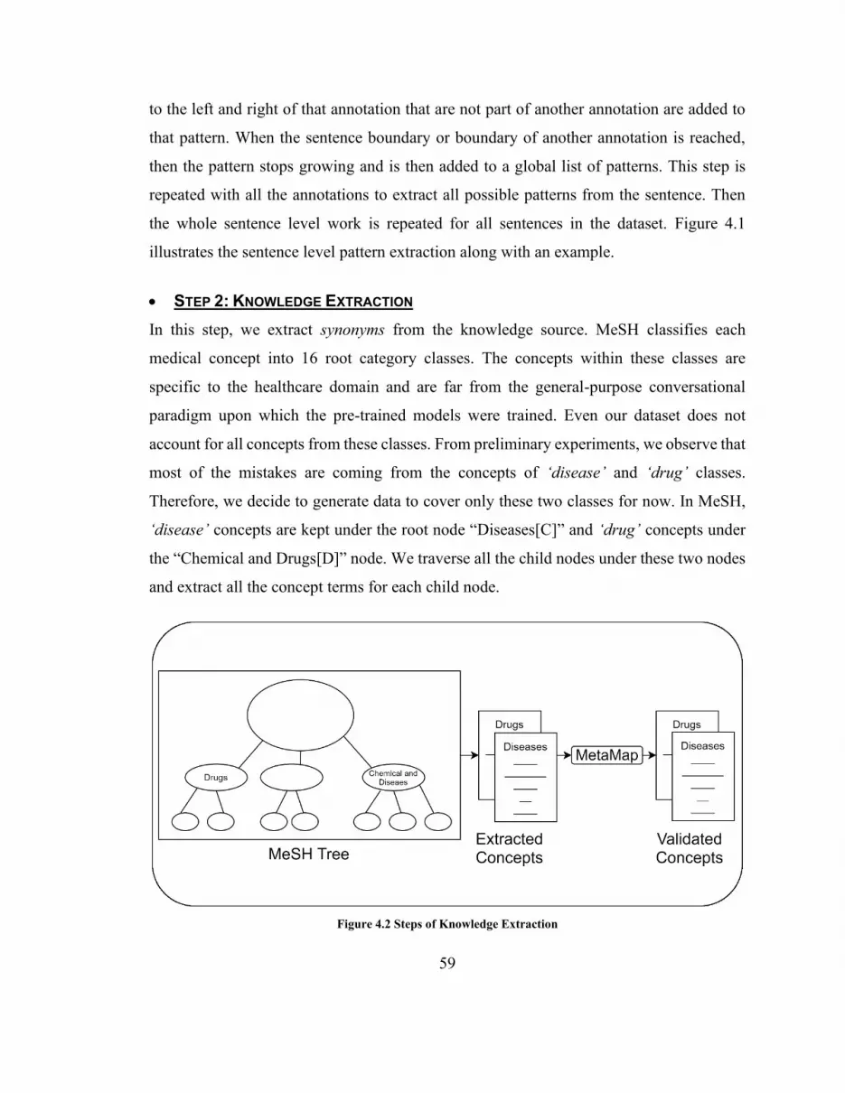
59

to the left and right of that annotation that are not part of another annotation are added to

that pattern. When the sentence boundary or boundary of another annotation is reached,

then the pattern stops growing and is then added to a global list of patterns. This step is

repeated with all the annotations to extract all possible patterns from the sentence. Then

the whole sentence level work is repeated for all sentences in the dataset. Figure 4.1

illustrates the sentence level pattern extraction along with an example.

• STEP 2: KNOWLEDGE EXTRACTION

In this step, we extract synonyms from the knowledge source. MeSH classifies each

medical concept into 16 root category classes. The concepts within these classes are

specific to the healthcare domain and are far from the general-purpose conversational

paradigm upon which the pre-trained models were trained. Even our dataset does not

account for all concepts from these classes. From preliminary experiments, we observe that

most of the mistakes are coming from the concepts of ‘disease’ and ‘drug’ classes.

Therefore, we decide to generate data to cover only these two classes for now. In MeSH,

‘disease’ concepts are kept under the root node “Diseases[C]” and ‘drug’ concepts under

the “Chemical and Drugs[D]” node. We traverse all the child nodes under these two nodes

and extract all the concept terms for each child node.

Figure 4.2 Steps of Knowledge Extraction

60

In MeSH, each medical concept enlists all candidate and qualifier terms, while defining a

separate list for the preferred terms of that concept. Many of these terms are closely related

to the concept but are not strictly synonymous with the terms that are in use by the

physicians. Moreover, root nodes of MeSH include all the concepts that are from all

domains of medical science, while for this work we are only interested in those concepts

that are applicable in the pediatric emergency departments. As an example, the “Chemical

and Drugs[D]” node contains a concept “Propoxur” which is an insecticide. “Propoxur” is

not related to pediatric care and is not applicable in our case. Therefore, it is required to

filter out such terms from our extracted lists to ensure that the terms are semantically

similar to our working domain. To filter the lists, we considered a validation step where

only those terms are validated and kept that are semantically closer to our dataset, and all

other terms were dropped.

To validate the extracted concepts, we passed each concept term to the Metamap and

examined the detected semantic type. If the semantic type matches those that are already

existing in our dataset while the semantic type belongs to the same root node from which

the term is coming, then we consider that term as valid. We collected all the valid terms

for each of the two semantic classes that we extracted. Figure 4.2 depicts the whole process

of knowledge extraction. After the extraction and validation of concepts, we get 24,071

concepts from the ‘disease’ class and 29,935 concepts from the ‘drug’ class.

• STEP 3: AUGMENTATION

In this step, we generate simulated data by using patterns and medical concepts extracted

in previous steps and then augment the simulated data with our original text corpus. Our

strategy in this step is similar to synonym replacement, with a small change that seeks

selection of concept list depending upon the class of concept within each pattern. For this

step, we know that each pattern has exactly one medical concept within it.

61

Figure 4.3 Steps to Generate Augmented Corpus

For each pattern from the patterns list, we check the class of the medical concept. If the

concept belongs to the ‘drug’ class, we select the list of drugs for the augmentation. In case

the concept belongs to the ‘disease’ class, we select the list of diseases. For anything else,

the pattern does not augment. To augment the pattern with the selected list of concepts,

each concept within the list is used to replace the existing concept in the pattern to form a

simulated variation. Each new variation after the replacement is then recorded in the list of

simulated patterns (Figure 4.3). These simulated patterns are then combined with the

original text corpus to form an augmented corpus.

Our data augmentation task enabled us to work with two datasets: original and augmented.

We use both datasets to evaluate our language modeling methods that we define in later

tasks. For the evaluations, we require data augmentation on multiple subsets of our original

dataset. Therefore, we develop a utility program using JAVA to automate the augmentation

process. Our utility program takes lists of concepts (Drugs and Diseases) and a text dataset,

and then it outputs the augmented dataset.

4.5.2 Developing Domain-Specific Language Models

In this task, we develop language models using only the domain-relevant data. For this

purpose, we use both datasets: original and augmented. Augmentation is done using the

62

methods presented in the previous task. Language models are created using the KenLM

toolkit.

KenLM provides methods to develop n-gram based language models in ARPA [117]

format. ARPA is a file format to list down all the calculated probabilities within an n-gram

language model. ARPA formatted models are bulky and not efficient to use for inferences;

hence, for efficient execution, it is required to convert ARPA models into specific data

structures [118]. KenLM also provides functions to convert the ARPA formatted models

into PROBING and TRIE data structure based language models [91]. PROBING data

structure is faster but uses extensive amounts of memory for inferences. In comparison, the

TRIE data structure aims to lower memory consumption. As our compute environment has

a limited stack of memory, we adapt the TRIE data structure to develop our language

models. Project DeepSpeech also supports TRIE structure by providing a native client to

convert the TRIE based language models into efficient binaries that aim speedy execution.

In this task, we use four steps to develop language models. In the first step, we streamline

the dataset by removing all leading and trailing whitespaces from all the sentences and

converting them into lower case. In the second step, the streamlined dataset trains an ARPA

based language model of the 5th order. We use the maximum n-gram order length of 5

because the pre-trained model from DeepSpeech uses the maximum of 5-grams; therefore,

we keep the n-gram order similar for valid comparisons. In the third step, the ARPA model

converts into a TRIE based model. Finally, the TRIE model converts into DeepSpeech

specific binary using its native client.

In this task, we develop language models in two strategies. In the first strategy, we directly

use the original dataset to develop the language models. In the second strategy, we apply

augmentation methods on our original dataset and then use the augmented dataset to

develop the language models.

63

4.5.3 Enhancing Pre-Trained Language Model

In this task, we enhance the pre-trained language model by incorporating information from

our domain-relevant dataset. There are two main reasons to seek this task for the

development of robust language models. The first reason is the insufficiency of our

domain-relevant dataset. We have only 127 kilobytes of text available in the original

dataset. Although after augmenting, we are able to generate about 2 gigabytes of text;

however, the pre-trained DeepSpeech model is trained on about 4 gigabytes of text, which

is still double. Therefore, we hypothesize that developing language models using text from

both data sources can be a better solution. The second reason is due to the preliminary

analysis, where DeepSpeech, with its pre-trained language model, made more critical

mistakes then general mistakes. From the nature of mistakes, we observed that the pre-

trained language model lacks domain-specific vocabulary, evidently due to its training

upon an out-of-domain data source. Therefore, we consider a reduction in critical errors by

introducing domain-relevant vocabulary in the pre-trained model.

Enhancement of the language model entails combining the information from other data

sources (domains) to the existing language model. Language models can be combined by

any of two methods: pooling and interpolation. In the pooling method, the corpus of the

existing language model is pooled with the text from other data sources. The pooled corpus

then trains an enhanced language model. In the interpolation method, a separate language

model is trained using the text from each data source. Afterward, all language models;

existing and newly trained, are merged using weights that are tuned on some validation

text. This validation text is fetched from the target domain.

The interpolation method has some variations [119]. The simplest of all is linear

interpolation, in which all intermediary language models (𝑃𝑖) are combined linearly using

tuned weights (𝜆𝑖) (Equation 3). These weights are tuned over the validation set such that

it maximizes the likelihood operator 𝑃(𝑊|𝐻) for the combined model.

64

Equation 3

𝑃(𝑊|𝐻) = ∑ 𝑃𝑖(𝑊|𝐻)𝜆𝑖

𝑖

KenLM [91] toolkit uses the log-linear interpolation method, which is a slight variation of

the linear interpolation method. In the log-linear interpolation method, individual models

are merged by applying weights as the power and multiplying the powered models

(Equation 4).

Equation 4

𝑃(𝑊|𝐻) = 1

𝑍𝜆(𝐻)∏ 𝑃𝑖(𝑊|𝐻)𝜆𝑖

𝑖

After merging all the models, to complete the interpolation probability, the product is

divided by a normalizing term 𝑍𝜆(𝐻) to ensure that the sum of all probabilities over words

W equals to 1. The normalizing term calculates the product of all words in the vocabulary

of all language models (Equation 5).

Equation 5

𝑍𝜆(𝐻) = ∑ ∏ 𝑃𝑖(𝑊|𝐻)𝜆𝑖

𝑖𝑊

To enhance the pre-trained language model, we experiment with both; pooling and

interpolation; methods. Similar to the previous task, we adopt strategies to use both

datasets; original and augmented. In total, we develop language models in four strategies,

by the combination of methods and datasets. In the first strategy, we use the original dataset

to enhance the pre-trained language model using the pooling method. In the second

strategy, the same dataset is used with the interpolation method. The third and fourth

strategies are similar to the first two, in terms of methods; however, we use augmented

dataset in these strategies.

65

When we use the pooling method, the source corpus of the pre-trained model is pooled

with the domain-specific text of our datasets, and then the pooled text trains new language

models. When we apply the interpolation method, the pre-trained model remains the first

intermediary model, while we train separate models from our datasets and interpolate all

intermediaries. All the models developed in this task are trained using the n-gram order of

5, which denotes the maximum n-gram length in the language model.

4.5.4 Summary

In the language modeling phase, we work on three tasks. In the first task, we focus on the

generation of artificial domain-relevant data using the principles of the synonym

replacement method. We define a three-step method that expects a text corpus to work on,

and in turn, it provides an augmented corpus. In the second and third tasks, we provide

strategies to develop language models by using both datasets; original and augmented. Both

tasks, in combination, develop six strategies to train language models.

1) Training a new language model using the original dataset.

2) Training a new language model using the augmented dataset

3) Enhancing the pre-trained language model using the original dataset using the pooling

method.

4) Enhancing the pre-trained language model using the augmented dataset using the

pooling method.

5) Enhancing the pre-trained language model using the original dataset using the

interpolation method.

6) Enhancing the pre-trained language model using the augmented dataset using the

interpolation method.

All these strategies seek the development of n-gram based language models that are of 5th

order.

66

4.6 Discussion

We consider our solution to be replicable in other domains where noise and domain

robustness is required, and there is insufficient relevant data available. In the acoustic

modeling method, we approached to fine-tune a general-purpose model. As this model is

generic, the same method can be applied in any other domain. However, to replicate our

language modeling methods, particularly the data augmentation, one will need to look for

the domain-specific knowledge sources and concept detection tools for the successful

adaptation of these techniques.

4.7 Conclusion

In this chapter, we present our explored techniques and developed methods to train robust

and domain-specific models. Our methods focused on those acoustically distorted and

sensitive scenarios where there is a shortage of domain-relevant data. We first did the

preliminary analysis using pre-trained models of DeepSpeech. We then developed acoustic

modeling and language modeling methods by taking insights from the analysis. The

acoustic modeling method sought domain adaptation of the pre-built model along with a

fine-tuning operation using our dataset. On the other hand, language modeling focus on the

generation of domain-relevant data. It worked on a three-step method to generate an

augmented dataset, and then it developed six strategies to develop robust language models.

67

Chapter 5. SPEECH RECOGNITION – EVALUATIONS

5.1 Introduction

This chapter provides a detailed evaluation of the methods that we presented in the previous

chapter. Evaluations were done in 2 phases. Figure 5.1 shows the flow of the experiments

that we executed for our evaluations.

Figure 5.1 Flow of experiments

5.2 Setup

5.2.1 Evaluation Phases

Our solution defines methods to enhance both, acoustic and language models within the

speech recognition system, therefore our evaluation strategy consisted of two phases.

1) In the first phase, methods pertaining to each model were evaluated in isolation.

When evaluating the acoustic modeling method (in Section 0), we used the pre-

trained language model for the experiments. Similarly, when evaluating language

modeling methods (in Section 5.4), we used the pre-trained acoustic model. For the

evaluations in this phase, we did experiments with both, training and testing data to

68

analyze the performance when models have seen everything as compared to unseen

environments. We did not use the testing results to tweak the models, therefore we

did not use any separate validation set to test the models in this phase.

2) In the second phase, we evaluated both models in combination. The best performing

models from the first phase were selected to perform evaluations in combination.

We did not evaluate low performing methods in this phase, particularly due to the

fact that the first step of evaluation already gave us such insights. Finally, in this

phase, we used our validation set to present the final validation of our trained

models.

5.2.2 Cross-Validation

We used 10-fold cross-validation throughout the evaluations. Since we used the same

dataset to train both: acoustic and language: models, a conventional method of cross-

validation where the dataset shuffles and split into folds each time before conducting an

experiment can cause problems; specifically in the second phase of evaluations where we

intend to use trained models in combinations. Due to the limited dataset, we also cannot

afford to set aside a testing dataset. Therefore, to ensure reliable and valid evaluations, we

performed the shuffling and splitting task once, and recorded all the folds. Afterward, we

supplied the same folds whenever an experiment used cross-validation.

5.2.3 Interpretation of Results

In the evaluations, we analyze the impact of our methods by examining the difference in

performance and comparing it to baselines. As speech recognition systems are primarily

evaluated on error rates, we will be considering Word Error Rate (WER) along with our

custom metric Critical Error Rate (CER) to measure the performance where a lower error

rate means better performance. However, all the crucial decisions are made on the basis of

CER. There are two ways to examine the difference in performance. One way is to examine

the absolute change in error rates, while the other is to check the relative change with

respect to the error rate of baseline. In our evaluations, we have considered both ways to

examine our results, however, attention is given to the relative performance differences.

69

5.3 Evaluating Acoustic Modeling

This section provides an evaluation of our acoustic modeling method. In this method, we

fine-tuned the pre-trained acoustic model with our dataset. Fine-tuning was done till 8

epochs. We stopped at the 8th epoch due to the continuous increase in testing error rates.

Cross-validation was used to calculate testing error rates. For each of the 10 folds, the pre-

trained model was separately fine-tuned, and the error rates from all folds were averaged.

This process was repeated at each epoch. Error rates for training cases were calculated

directly by using the whole dataset for fine-tuning and using the same data to calculate

errors. Figure 5.2 shows the trend of errors on each epoch (horizontal axis) for both error

rates (vertical axis) and Table 5.1 lists down the values of error rates

Figure 5.2 Error loss in Acoustic Model training

70

Table 5.1 Training and testing error rates for Acoustic Model training

CER WER

Training CV Testing Training CV Testing

nth

Ep

och

1 27.59% 38.09% 26.84% 36.94%

2 19.62% 32.31% 19.43% 32.04%

3 16.47% 29.57% 16.56% 29.77%

4 13.06% 27.42% 13.53% 27.83%

5 12.57% 27.45% 12.94% 28.11%

6 10.84% 27.22% 11.47% 28.01%

7 9.25% 28.17% 9.84% 28.86%

8 9.37% 28.35% 9.75% 29.28%

5.3.1 Analysis

Analysis of error rates in comparison with the number of epochs showed that the model

reached a local minima on our dataset on around 4th to 6th epochs. Our analysis of the error

rates shows that the 6th epoch is the most efficient (CER: 27.22%) on the basis of CER,

while the 4th epoch is the most efficient (WER: 27.83%) on the basis of WER. With the

fine-tuning method, we were able to achieve 22.16% absolute and 44.88% relative

reduction in CER and 18.8% absolute and 40.32% relative reduction in WER (Table 5.2).

As the performance comparison was very close (error difference within a range of 0.2%),

models from the 4th to 6th epoch were selected for further evaluations of the second phase.

Table 5.2 Absolute and relative change in error rates after acoustic modeling

CER WER

Pre-trained AM 49.38% 46.63%

Pre-trained AM + fine-tuning 27.22% 27.83%

└ Absolute change -22.16% -18.80%

└ Relative change -44.88% -40.32%

71

5.4 Evaluating Language Modeling Methods

This section provides an evaluation of our language modeling methods. We provided six

strategies to train domain-relevant language models for improved recognition. In our

evaluations, we combined all those strategies to develop 8 evaluation scenarios that cover

all methods. Table 5.3 provides the details of each evaluation scenario.

Table 5.3 List of scenarios for Language Model evaluations

S.

No. Evaluation Scenario Strategy Details

1 Pre-trained LM Baseline: Performance from the preliminary

experiment is considered.

2 No LM No LM is used in this scenario.

3 New LM

+ Original in-domain corpus

New LM is trained using the text corpus from

the original in-domain dataset.

4 New LM

+ Augmented in-domain corpus

New LM is trained using the text corpus from

the augmented in-domain dataset.

5

Pre-trained LM

+ Original in-domain corpus

+ Pooling Method

Pre-trained LM is enhanced using the text

corpus from the original in-domain dataset

using the pooling method.

6

Pre-trained LM

+ Original in-domain corpus

+ Interpolation Method

Pre-trained LM is enhanced using the text

corpus from the original in-domain dataset

using the interpolation method.

7

Pre-trained LM

+ Augmented in-domain corpus

+ Pooling Method

Pre-trained LM is enhanced using the text

corpus from the augmented in-domain dataset

using the pooling method.

8

Pre-trained LM

+ Augmented in-domain corpus

+ Interpolation Method

Pre-trained LM is enhanced using the text

corpus from the augmented in-domain dataset

using an interpolation method.

72

Scenario 1 was developed to provide a baseline for this evaluation; therefore, we did not

run any experiments in this scenario; instead, the results from preliminary experiments

were considered. Scenario 2 was developed to test the performance of DeepSpeech without

the use of any language model, as it is not a required component in speech recognition. For

the experiments within this scenario, all audio clips from our original dataset were used to

calculate error rates. In all other scenarios, language models were trained and tested using

training and testing datasets. While evaluating the training error rates, language models

were trained using the whole text corpus from the original dataset and all audio clips from

the same dataset were used to test those models. While evaluating testing error rates, we

used 10-fold cross-validation.

5.4.1 Analysis

The analysis of our results shows that DeepSpeech did mistakes for more than half the time

in scenario 2 when no language model was used. Upon comparing the error rates with

baseline, one can see that the average CER increased around 8% and WER increased

around 10% when DeepSpeech did not use any language model. This provides evidence of

the importance of language models in the process of speech recognition. Moreover, when

such language models were used that has already seen the testing data while training, the

recognition performance matched the top of the line cloud-based SR (Google). This is not

a valid comparison to build a conclusion; nevertheless, it highlights the ability of language

models to significantly boost the recognition performance. Table 5.4 shows the error rates

for all scenarios when the training dataset was used to test the models that were trained

using the corpus from the same dataset. The table also shows error rates from the first 2

scenarios to provide a comparison, even though no language model was trained in those

scenarios.

73

Table 5.4 Training error rates from each evaluation scenario

Table 5.5 Cross-validated error rates from each evaluation scenario

74

Cross-validated experiments show that all our methods improved DeepSpeech

performance since we observe lower error rates as compared to the baseline in each

experimented scenario. We note a maximum absolute reduction of 4.81% WER and 9.9%

CER in our experiments, which translates into a 10.31% relative reduction in WER and

20.04% CER. Table 5.5 presents a bar chart plot and values of error rates in each scenario,

while Table 5.6 lists the absolute and relative differences as compared to the baseline.

Table 5.6 Absolute and relative change in error rates compared to baseline

Evaluation

Scenario

Critical

Error

Rate

Absolute

Difference

(CER)

Relative

Difference

(CER)

Word

Error

Rate

Absolute

Difference

(WER)

Relative

Difference

(WER)

Baseline

Pre-Trained LM 49.38% 0.00% 0.00% 46.63% 0.00% 0.00%

New LM

+ Original corpus 39.49% -9.9% -20.04% 41.82% -4.81% -10.31%

New LM

+ Augmented corpus 45.05% -4.33% -8.77% 43.10% -3.53% -7.57%

Pre-trained LM

+ Original corpus

+ Pooled

47.12% -2.26% -4.59% 45.03% -1.6% -3.43%

Pre-trained LM

+ Original corpus

+ Interpolated

42.40% -6.98% -14.13% 43.28% -3.35% -7.18%

Pre-trained LM

+ Augmented corpus

+ Pooled

47.04% -2.35% -4.75% 44.56% -2.07% -4.43%

Pre-trained LM

+ Augmented corpus

+ Interpolated

44.02% -5.36% -10.86% 42.76% -3.87% -8.29%

75

As we presented multiple methods that are applied in combination with each evaluation

scenario, we were interested in analyzing the impact of each individual method on the

performance of DeepSpeech. Therefore, we defined four independent variables based on

our methods, whose values represent results from each experimented scenario. Table 5.7

lists all variables and their values along with the scenarios that are represented by each

value combination. We assigned the value 1 to denote a True or ‘Yes’, meaning that the

respective variable was applied to the scenario, whereas, the value 0 denotes False or ‘No’.

Table 5.7 Variables to analyze each experimented method

Variables → Augmentation

of Original corpus

Development of in-domain

LM

Enhancement of Pre-Trained

LM using Pooling

Enhancement of Pre-Trained

LM using Interpolation

Evaluation Scenario ↓

3 0 1 0 0

4 1 1 0 0

5 0 0 1 0

6 0 0 0 1

7 1 0 1 0

8 1 0 0 1

Based on these variables, we analyzed the contribution of each method in improving the

performance of DeepSpeech. For this analysis, we applied linear regression where the null

hypothesis is that there is no change in performance within the different experimented

scenarios. Our analysis used only three of these variables since we had to drop the use of

variable “Development of in-domain LM” due to its direct correlation with other

enhancement variables (“Enhancement of Pre-Trained LM using Pooling” and

“Enhancement of Pre-Trained LM using Interpolation”). In scenarios 3 and 4, we

experimented with the methods that are based on the dropped variable; however, values

from other variables are still able to represent these scenarios (False for both of

enhancement variables translates into a True for dropped variable). We applied regression

analysis on both error rates individually by keeping them as the dependent variables. Figure

5.3 shows the results summary of regression analysis when WER is taken as the predicted

variable. Figure 5.4 shows the results summary of regression analysis for CER. In total 6

76

scenarios were compared each having 100 observations, therefore the summaries have

shown 600 observation count.

Figure 5.3 Result summary of regression analysis using WER

Figure 5.4 Result summary of regression analysis using CER

The ANOVA results from regression analyses reject the null hypothesis when CER is taken

as the performance factor, which provides the domain-specific error rate. Due to the

importance of critical errors, we argue that some of our methods have a significant impact

on the performance of recognition than others, even when there does not seem to have a

significant difference in general word errors. However, in these analyses, we were not able

to support any single method in providing a significant contribution to error reduction.

Therefore, we investigated more on our results to see the combined effects of our methods.

77

We firstly analyzed the results of those scenarios that applied the augmentation method to

compare with those scenarios that used original datasets. We observe that the augmentation

method increased error rates as compared to those language models that were created only

with our original dataset corpus. However, in those scenarios where we were enhancing

the pre-trained language model, the augmentation method did show some reduction in error

rates. We noted a maximum of 1.19% relative reduction in WER and 0.18% relative

reduction in CER; however, these reductions are not reliable, as we also observe substantial

increase (3.81% relative) in critical errors when enhancement is done using an interpolation

method. Table 5.8 mentions absolute and relative differences between all scenarios using

original and augmented datasets.

Table 5.8 Comparing error rates between original and augmented corpus

CER WER

New

LM

Pre-

Trained

LM

+Pooling

Pre-Trained

LM

+Interpolation

New

LM

Pre-

Trained

LM +

Pooling

Pre-Trained

LM

+Interpolation

Original corpus 39.49% 47.12% 42.40% 41.82% 45.03% 43.28%

Augmented corpus 45.05% 47.04% 44.02% 43.10% 44.56% 42.76%

└Absolute Diff. 5.57% -0.08% 1.62% 1.28% -0.47% -0.52%

└Relative Diff. 14.10% -0.18% 3.81% 3.05% -1.03% -1.19%

Secondly, we analyzed all those scenarios which train new language models to compare

with those scenarios that enhance the pre-trained model using the pooling method as well

as those using the interpolation method. We note that enhancement, in general, is not

effective in reducing error rates; however when interpolation is used to enhance the pre-

trained model, we observed 2.29% relative reduction of CER and 0.78% of WER using the

augmented corpus. From all other scenarios, a new language model using only the original

(un-augmented) corpus gave us the lowest error rates. Table 5.9 and Table 5.10 lists the

absolute and relative differences in error rates when using pooling and interpolation

methods in comparison to the new domain-specific language modeling method.

78

Table 5.9 Comparing error rates between new and enhanced pooled model

CER WER

Using

Original

Corpus

Using

Augmented

Corpus

Using

Original

Corpus

Using

Augmented

Corpus

New LM 39.49% 45.05% 41.82% 43.10%

└Enhanced LM using Pooling 47.12% 47.04% 45.03% 44.56%

└Absolute Difference 7.63% 1.98% 3.21% 1.46%

└Relative Difference 19.33% 4.40% 7.67% 3.40%

Table 5.10 Comparing error rates between new and enhanced interpolated model

CER WER

Using

Original

Corpus

Using

Augmented

Corpus

Using

Original

Corpus

Using

Augmented

Corpus

New LM 39.49% 45.05% 41.82% 43.10%

└Enhanced LM using Interpolation 42.40% 44.02% 43.28% 42.76%

└Absolute Difference 2.92% -1.03% 1.46% -0.33%

└Relative Difference 7.39% -2.29% 3.48% -0.78%

To sum up our analysis, we observe three key performance behaviors of our methods. 1)

The pooling method to enhance the pre-trained model has the least impact on the reduction

of error rates. 2) The application of the augmentation method on our original dataset,

however, did enhance the impact of the pooling method, yet it was not able to surpass the

standalone impact of the interpolation method. 3) Nevertheless, the development of simple

domain-specific language models has the highest impact, although, enhancement of the

pre-trained model seems a more logical option as it provides an opportunity to generate

models that are trained on a larger set of information.

To understand these behaviors, we analyzed the construction of the clinical notes from our

dataset i.e., our target domain. In the notes, we observe many patterns that were recurring

79

in almost the whole dataset. An instance that we observe that usually occur in the start of

every note is, “This is a <age> <weeks/month/year> old <white/black/other ethnicity>

<male/female> …”. Some examples that follow this pattern are; “This is a 2 months old

white male …”, “This is a 4-year-old black female ...”. Due to many of such patterns that

physicians mostly follow while dictating notes, a language model needs to learn them in

order to perform efficient recognition. If there happens to be a glitchy output from the

acoustic side, a language model will only be able to refine that output if it is already aware

of such patterns. The main purpose of language model training is, in fact, to pick the

recurring patterns from the training set. Therefore, when we talk about the pre-trained

model, it implies that this model has already identified patterns from the datasets on which

it was trained. Hence, when we try to enhance the pre-trained model, we try to teach it

some new patterns. The pre-trained model was trained on about 4 gigabytes of text,

whereas the text from our original dataset all combined is not more than 150 kilobytes.

Therefore, we consider that our smaller text corpus was not able to make a significant

impact while enhancing the pre-trained model due to the smaller size. The property of the

pooling method to give equal weight to all data sources also supports this idea. This also

explains the increased impact of error reduction by the use of the augmentation dataset, as

it increases the size of the domain-relevant text corpus.

After analysis, we selected language models from all scenarios for the second phase

experiments, except those scenarios that implement the pooling method. We dropped the

pooling method for further evaluations due to two main reasons. Firstly, it has shown the

least performance gains, as we have mentioned above. Secondly, pooling is one of the two

model enhancement methods that we experimented with; therefore, we only wanted to

continue with one best method of enhancement.

80

5.5 Combined Evaluation

In this section, we provide our second phase of evaluation. In this phase, no new model

was trained, instead, the best performing models; that we selected from previous

evaluations; were analyzed further. We selected multiples of both: acoustic and language;

models and tested all their combinations on our original dataset using the same cross-

validation folds upon which the models were trained. Table 5.11 lists the error rates for all

tested combinations in this evaluation phase.

Table 5.11 Error rates after testing with combined models.

CER WER

Acoustic Model → 4th Epoch 5th Epoch 6th Epoch 4th Epoch 5th Epoch 6th Epoch

Language Model ↓

Pre-trained LM

+ Original Corpus

+ Interpolated

26.55% 26.04% 25.51% 28.30% 28.12% 27.90%

Pre-trained LM

+ Augmented Corpus

+ Interpolated

25.73% 25.89% 25.17% 26.97% 27.41% 26.95%

New LM

+ Original Corpus 24.03% 24.28% 24.05% 27.18% 27.51% 27.35%

New LM

+ Augmented Corpus 26.65% 26.10% 25.74% 27.13% 27.49% 27.23%

5.5.1 Analysis

The combined evaluation showed that we achieved the lowest word error rate (WER:

26.95%) from the combination of the acoustic model of the 6th epoch and the pre-trained

language model that is enhanced using augmented corpus. However, this model

combination was slightly behind with respect to critical error rates. The lowest critical error

rate (CER: 24.03%) was achieved by the 4th epoch acoustic model in combination with a

new language model that was trained using only the original dataset.

The analysis of results shows that the language modeling methods of dataset augmentation

and model interpolation works best in combination to reduce general error rates. In terms

81

of WER, the augmented interpolated language models performed better than standalone

augmented and standalone interpolated models and were also the overall best performing

models.

Table 5.12 Performance comparison of DeepSpeech (before and after) with Google

When analyzing critical errors, we found that the 4th epoch acoustic model did less critical

mistakes when combined with new language models, and the 6th epoch acoustic models

did less critical mistakes with interpolated language models. However, the lowest critical

error rate was achieved by newly trained language models on the original dataset. The

augmented interpolated language models were the second-lowest with about 4.7% relative

difference.

82

In the end, we found that all of our acoustic and language modeling methods, in

combination, were able to significantly improve the performance of DeepSpeech by

reducing error rates from 46.63% to 26.95% WER and from 49.38% to 25.17% CER. This

reduction relatively translates into a 42.2% reduction in WER and 49.02% in CER. This

improvement enables DeepSpeech to deliver performance that is relatively close to the

performance of top-of-the-line cloud-based SR (Google). Table 5.12 shows the error rates

of Google, DeepSpech before applying our methods and DeepSpeech after applying our

acoustic and language modeling methods.

5.6 Working Examples

In this section, we have provided examples of critical and word errors within the

transcribed notes that we observed with the best performing model combinations. In this

section, we present a best-case examining transcribed note with the least critical errors, a

worst-case examining a note with the most critical errors and two random cases. The two

model combinations that we are examining are 1) 4th epoch acoustic model and new

language model with the original corpus, and 2) 6th epoch acoustic model and enhanced

pre-trained language model with the augmented corpus.

5.6.1 Best Case

In all our 100 notes, the best-transcribed note achieved a CER as low as 6.25% with the 1st

model combination where it made only 5 critical mistakes out of 80 total critical concepts.

With the 2nd model combination, it achieved 7.5% CER and made 6 critical mistakes. The

quality of the corresponding speech in the audio note is found to be clear without any

background noise. The dictation is at a normal pace and it appears to be recorded in a closed

room with a relaxed environment. Almost all critical mistakes, in this case, were found to

be homonyms. For example, “enterovirus” was mistaken as “ether is” and “two older” as

“told or”. Table 5.13 lists transcriptions from both model combinations. All the highlighted

and bold words and phrases are the errors. The yellow highlights are general word errors,

while green highlighted and underlined are critical errors.

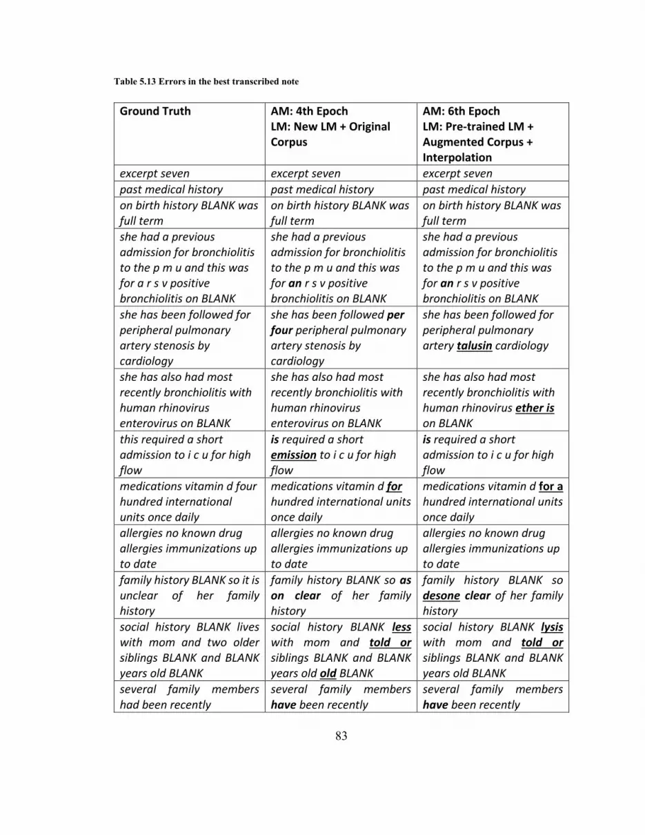
83

Table 5.13 Errors in the best transcribed note

Ground Truth AM: 4th Epoch LM: New LM + Original Corpus

AM: 6th Epoch LM: Pre-trained LM + Augmented Corpus + Interpolation

excerpt seven excerpt seven excerpt seven

past medical history past medical history past medical history

on birth history BLANK was full term

on birth history BLANK was full term

on birth history BLANK was full term

she had a previous admission for bronchiolitis to the p m u and this was for a r s v positive bronchiolitis on BLANK

she had a previous admission for bronchiolitis to the p m u and this was for an r s v positive bronchiolitis on BLANK

she had a previous admission for bronchiolitis to the p m u and this was for an r s v positive bronchiolitis on BLANK

she has been followed for peripheral pulmonary artery stenosis by cardiology

she has been followed per four peripheral pulmonary artery stenosis by cardiology

she has been followed for peripheral pulmonary artery talusin cardiology

she has also had most recently bronchiolitis with human rhinovirus enterovirus on BLANK

she has also had most recently bronchiolitis with human rhinovirus enterovirus on BLANK

she has also had most recently bronchiolitis with human rhinovirus ether is on BLANK

this required a short admission to i c u for high flow

is required a short emission to i c u for high flow

is required a short admission to i c u for high flow

medications vitamin d four hundred international units once daily

medications vitamin d for hundred international units once daily

medications vitamin d for a hundred international units once daily

allergies no known drug allergies immunizations up to date

allergies no known drug allergies immunizations up to date

allergies no known drug allergies immunizations up to date

family history BLANK so it is unclear of her family history

family history BLANK so as on clear of her family history

family history BLANK so desone clear of her family history

social history BLANK lives with mom and two older siblings BLANK and BLANK years old BLANK

social history BLANK less with mom and told or siblings BLANK and BLANK years old old BLANK

social history BLANK lysis with mom and told or siblings BLANK and BLANK years old BLANK

several family members had been recently

several family members have been recently

several family members have been recently

84

5.6.2 Worst Case

In our results, the worst transcription achieved the CER of 59.6% with 2nd model

combination and 54.8% CER with 1st model combination. We observed that the quality of

the corresponding audio note is significantly lower than other notes. We note high echo

and reverberation in the audio while appearing that the speaker is away from the recording

device. This audio note was also filled with a high amount of background noise, especially

the overlapping noise that is corrupting the speech signals. We hear loud baby cries and

parents trying to soothe the baby in the background by talking and playing with the baby.

These interruptions reflect on the mistakes. For example, in one place “abdominal pain” is

mistaken as “a dona panadol”. This transcription is not a homonym for its gold standard.

Another similar example is when “upper respiratory tract infection” transcribes into “offer

reichstein”. These examples show that due to overlapping noise, a lot of speech signal is

lost, resulting in a sloppy transcription. Table 5.14 presents the comparison of

transcriptions for both model combinations. Green highlights show critical mistakes.

Table 5.14 Errors in the worst transcribed note

Ground Truth AM: 4th Epoch LM: New LM + Original Corpus

AM: 6th Epoch LM: Pre-trained LM + Augmented Corpus + Interpolation

this is a four year almost

five year old female with

trisomy twenty one

he is a four year always

five year old female at ten

twenty one

he is a four year as five

year old female as try

twenty one

presenting with two to

three week history of upper

respiratory tract infection

that has lingered

awakening with a cough

and having the cough

during the day and

sometimes at night

is an in a to the three

weeks history as offer

rather infection of lines

waiting with her cough

and having (the) cough

during the day and some

time at night

is anion so to three weeks

history as offer reichstein

of linear waiting with call

and having (the) cough

during the day had some

time (at) tight

ventolin of no benefit

recently

that on no better we that on no batel rashes

she has had no fevers with

this

she (has) had no fevers

with this

(she has) at no fevers with

this

85

possible headache no other

pain

four headache nor her

pain

four endantadine

she has had abdominal

pain and vomiting a week

ago that resolved over

about a day and resulted in

multiple episodes of

vomiting

she has had a do paid

(and) vomiting a week no

that resolved over about a

vein (and) result is well

colitis following

she has had a dona

panadol in a week no the

resolved over about ada in

result as well colicines

following

she has been on p o

steroids for the last five

days as per the parents

usual approach to acute

asthma

she says on p o per i for

(the last) five days her the

parents usual got his used

for as no

she see n p o ser for (the

last) five days her the

parents usual proctocele

for as mopeg

paragraph past medical

history immunizations are

up to date

paragraph past medical

history immunizations are

(up to) date

ph past medical history

immunizations (are) up to

date

she has had a tetralogy of

fallot repaired trisomy

twenty one and she is on

valproic acid and

clobazam for seizure

disorder which is quiescent

for the last two years

ten had also or care

trisomy twenty one and she

(is) on a for acid episode

for (seizure disorder)

which is a two years

on fenoterol some or

paired trisomy twenty one

and she (is) on dolo acidic

anorectics two years

on exam no respiratory

stress normal air entry

with no wheeze airway

breathing and circulation

stable

on exam no respiratory

stress normal artery with

no wheezer we breathing

in certain stable

on exam no respiratory

stress normal reentry with

no leader we breathing and

circulation stable

pink soft belly normal left

ear normal right ear

pain saw a day normal as

ear nor rays

pain sagatal normal last

ear nor river

snotty nose but not

dramatically swollen

tonsils, slightly red, no pus.

not dramatically acute

not of note a iron in last or

or to widened no refused

to one week ago i saw so

so i group is probably a

mild mild being a certain

in wide per were more

operation the in are work

but i do an a b released

nodose but no oestro

intraorbital red neural

perforin was miosis so so

iridoids probably mild

iletin ceresan viper werner

osteoid an a b q resin

86

5.6.3 Random Cases

We chose two random notes, in between the above-presented best and worst cases, to

analyze the mistakes. Upon examining the corresponding audio recordings, we found that

the noise levels remained between the above-defined two example cases. There were no

overlapping noises, however, we could listen to some reverberation. On a few occasions,

the physician’s dictation pace increased dramatically, which directly increased mistakes in

transcriptions. On one of such occasions, the phrase “feet swept out from underneath him”

was mistaken as “feet slept out from under eat him”.

The first random note we examined achieved 11.66% CER with the 1st model combination

and 14.4% CER with 2nd model combination. Table 5.15 mentions the transcription we

received with both model combinations.

Table 5.15 Errors in the first examined note transcription

Ground Truth AM: 4th Epoch LM: New LM + Original Corpus

AM: 6th Epoch LM: Pre-trained LM + Augmented Corpus + Interpolation

this is an eighteen month old black female

this is a ten month old black female

this is a ten month old black female

presenting with a seizure like episode at home

presenting with a seizure like episode at home

presenting with a seizure like episode at home

child was perfectly well until three days ago when sniffles and cough became apparent

child was perfectly well until three days ago when sniffles and cough became apparent

child was perfectly well until three days ago when sniffles and cough became apparent

last evening at about eighteen hundred hours the child experienced a mild fever of thirty eight point five

last evening (at) about eighteen hundred hours the child experience on mild (of) fever thirty eight point five

last evening (at) about eighteen hundred hours the child experience a mild fever (of) thirty eight point five

this morning on rousing her from her bed and she stiffened exhibited five to fifteen seconds of shaking movements suggestive of

this morning on rising her for her bed if she stiffened excited five to fifteen seconds of of shaking movement suggestive of

this morning on the rising her for her bed if she stiffened excited five to fifteen seconds of of shaking movement

87

tonic clonic seizure and then settled into a deep sleep from which she roused fifteen minutes later

tonic clonic seizure and in settled into a deep sleep for which she was fifteen minutes later

suggestive of tonic clonic seizure and intensain to a deep sleep for which she resistin in the later

by the time she arrived at the i w k emergency she was awake and alert and cranky

in time she wrist the i w k emergency is she was awake and alert and cranky

date she arrived at the i w k emergency i she was awake and alert and cranky

parents have never seen similar seizure activity before

parents have never seen similar seizure activity before

parents have never seen similar seizure activity before

past medical history reveals immunizations up to date and normal birth and pregnancy history with no specialist and no regular medications and no known allergies

past medical history revealed immunizations up to date a normal birth and pregnancy history with no specialists and no regular medications and no known allergies

past medical history reveals immunizations up to date a normal birth and pregnancy history with no specialist and no regular medications and no known allergies

family history reveals febrile seizures in dad as a child

family history reveals febrile seizures in dad as a child

family history reveals febrile seizures in dead as a child

physical exam revealed a cranky child who settled with care

physical exam revealed a cranky child who settled with care

physical exam revealed a cranky child who settled with care

ear nose and throat exam revealed a red throat with no exudate suggestive of a viral pharyngitis

ear nose and throat exam revealed a red throat with no x date suggestive of a viral pharyngitis

ear nose and throat exam revealed a red throat with no exo date suggestive of a viral paris

ears were normal lungs were clear

ears were normal lungs were clear

ears were normal lungs were clear

cardiac exam was unremarkable

cardiac exam was unremarkable

cardiac exam was unremarkable

abdominal exam was normal

abdominal exam was normal

abdominal exam was normal

neurological exam revealed a child who following ibuprofen was playful and interactive and no focal finding on

neurological exam revealed a child who following ibuprofen was playful and interim and no focal findings on

neurological exam revealed a child who following ibuprofen was playful and interacting and no focal findings under local exam is cover

88

neurological exam was discovered

neurological exam is descend

new paragraph impression is that this is simple febrile seizure

new paragraph impression is that this is simple febrile seizure

new paragraph impression is that this is simple febrile seizure

parents were counseled and reassured

parents were counseled and reassured

parents were counseled and reassured

instructions were given with regards to the delivery of ibuprofen as needed for pain and fever but the parents were cautioned that this would not reduce the risk of further seizures.

instructions were given with regards to the delivery of ibuprofen as needed for pain and fever by the parents were cousin that this would not reduced the risk of for other seizures

instructions were given with regards to the delivery of i do provided for pain and fever but the parents were cation that this would not reduced the rose of further seizures

we stated the seizure risk at about one or two percent over the rest of this illness

we stayed the seizures (risk) at about one or two percent over the rest of the illness

we state the seizure risk at about one or two percent over the rest of the sinus

but cautioned them that further febrile seizures were likely between now and six years of age

but out on them that further febrile i sure were likely between now and six years of age

but cation them that further febrile tissue (were) likely between no and six years of age

her parents were advised to return to the emergency department with further seizures for further assessment

a parents were advised to return to the emergency department with rather seizures refer her assessment

a parents were advised to return to the emergency department with further seizures refer assessment

diagnosis viral upper respiratory tract infection with febrile seizure

diagnosis for upper respiratory tract infection with febrile seizures

diagnosis boro upper parry tract infection with febrile seizure

89

The second random note we examined achieved 22.41% CER with the 1st model

combination and 24.13% CER with 2nd model combination. Table 5.16 shows the

transcription of the second random note we examined.

Table 5.16 Errors in the second examined note transcription

Ground Truth AM: 4th Epoch LM: New LM + Original Corpus

AM: 6th Epoch LM: Pre-trained LM + Augmented Corpus + Interpolation

excerpt thirty one excerpt thirty one excerpt thirty one

medications at admission medications at admission medications at admission

two hundred and fifty

milligrams of amoxil t i d

for ten days started on

BLANK

to turn fifty milligrams of a

lot p i d for ten days see on

BLANK

to endrin fifty milligrams of

a moban t i d for ten days

are on BLANK

examination at admission examination and admission examination and admission

BLANK was afebrile and

vitally stable

BLANK is a febrile advised

this table

BLANK was a febrile and

vita e table

head and neck exam was

unremarkable cervical

lymph nodes were palpable

and less than one point five

centimeters in diameter

head and neck exam was

unremarkable service

lymph nodes with health

able and less than one point

five centimeters and via

head and neck exam was

unremarkable service

lymph nodes but palpable

and less than one point five

centimeters and dia

cardiac exam was normal cardiac exam was normal carb exam was normal

respiratory exam showed

increased work of

breathing

respiratory exam showed

increased work of everting

respiratory exam showed

increased work of retin

intercostal indrawing on

the right side

intercostal indrawing on

the right side

intercostal in von on vit

side

good air entry bilaterally

and course crackles and

wheezes throughout both

lung fields

a good air entry bilaterally

and course crackles one a

throat business

a good air entry bilaterally

and coarse crackles and

tear out pulseless

her abdominal exam was

unremarkable

her abdominal exam was

unremarkable

her abdominal exam was

unremarkable

allergies none allergies non allergies on

immunization status immunizations status immunizations status

90

After reviewing the individual cases, we observed that DeepSpeech was able to understand

the domain-specific speech for the most part. However, we noted 3 factors that are

prominently linked with the errors.

1) Reverberation

On average our dataset has low levels of reverberation. However, those audio notes

having high reverberation are consistently linked with high numbers of errors.

2) Overlapping Noise

Similar to reverberations, most of the notes in our dataset have moderate noise levels

that do not interfere with the speech. Therefore, such instances skew the performance

of transcriptions to a large extent.

3) Dictation Pace

Within the notes, we observed that the commonly occurring phrases are uttered at a

high pace, while complicated sentences are uttered slowly. However, when the speech

pace is up, transcription starts to show errors mostly by skipping critical words.

91

5.7 Final Validation

In this section, we report the results of our acoustic and language models on a separate

validation dataset. In the process of dataset preparation (Section 3.4.2), we separated a

validation set that we did not use in any of our prior experiments. Therefore, in this final

validation, we used our validation dataset upon all of our selected models, which were

trained from the whole original dataset. Table 5.17 lists the error rates for all model

combinations.

Table 5.17 Error rates on the validation dataset

CER WER

Acoustic Model → 4th Epoch 5th Epoch 6th Epoch 4th Epoch 5th Epoch 6th Epoch

Language Model ↓

Pre-trained LM

+ Original Corpus

+ Interpolated

32.09% 30.52% 30.41% 35.99% 34.39% 34.65%

Pre-trained LM

+ Augmented Corpus

+ Interpolated

33.24% 32.04% 33.30% 35.20% 34.23% 35.02%

New LM

+ Original Corpus 30.98% 29.63% 28.96% 34.99% 34.14% 33.84%

New LM

+ Augmented Corpus 34.30% 33.89% 34.61% 35.70% 35.34% 35.79%

We observed similar behaviors from the results of the final validation. With respect to

WER, the lowest error rates were from the enhanced pre-trained models that use the

augmented dataset and newly trained models on the original dataset. The lowest two error

rates from these language models only had an absolute difference of 0.09%. However, with

respect to CER, we found that newly trained models on the original dataset did a relative

maximum of 5% less critical mistakes then the enhanced pre-trained models.

92

5.8 Discussion

Throughout the evaluations, we observe that newly trained language models on our original

(un-augmented) dataset were performing similar to, or sometimes better than those

language models that apply our augmentation and model enhancement methods,

specifically in regard to critical errors. We consider that this was due to the extremely small

size of our dataset, which impacts the performance in two ways.

1) Language modeling is all about vocabulary and speech patterns. Thus, the small size

of our dataset does not cover both aspects sufficiently to reflect the target domain. We

tried to handle the vocabulary aspect by dataset augmentation method; however, we

were not able to introduce more domain-specific speech patterns.

2) The pre-trained model is trained on a significantly larger dataset than ours. Moreover,

when our small dataset breaks down into folds for cross-validation, it creates many

unseen scenarios for the testing. Thus, all those unseen domain-specific speech patterns

get compensation by the prior knowledge of the pre-trained model, which does not

reflect our target domain.

In addition to these two reasons, our limited implementation of the augmentation method

also hinders the reduction of critical errors. Since our definition of critical errors entails all

the domain-specific vocabulary, yet we only used two domain-specific classes (drugs and

diseases) to augment our augmentation method. Therefore, all the concepts of remaining

domain-specific classes also remain unseen in the experiments with testing folds.

The interpolation method that develops a language model using information from multiple

data sources has the ability to adjust in case the volume of data is not similar across all

sources. As there is a huge size difference in the data source of the pre-trained language

model and our dataset, the interpolation method logically has the means to cope up in this

situation. However, interpolation requires a separate tuning set from the target domain to

calculate weights for each data source. Since our dataset is already limited, fetching a

tuning set from it makes it even smaller. Therefore, we found that in our experiments the

93

interpolation method performed fairly closer to stand-alone models, but they were not able

to surpass the performance. Had we had a slightly larger dataset; we consider that the

interpolation method would have been the best in performance.

5.9 Conclusion

This chapter presents an evaluation of our defined methods. We have shown that by using

the fine-tuning method on the pre-trained deep speech acoustic model, WER relatively

decreased by 40.32% CER by 44.88% on our original dataset. After applying the data

augmentation method to our dataset and using the interpolation method to enhance the pre-

trained language model, we managed to reduce the error rates further relatively by 42.2%

WER and 49.02% CER. In our evaluations, we observed that the pooling method to

enhance the pre-trained language model had the least impact on the reduction of error rates.

Furthermore, when we applied our language modeling methods in isolation, neither of

those methods had a reducing impact on error rates. However, when applied in

combination, we observed lower error rates when the pre-trained language model was

enhanced using the interpolation method and augmented dataset.

94

Chapter 6. CLASSIFICATION OF TRANSCRIPTION INTO

SOAP CATEGORIES

6.1 Introduction

This chapter presents our work to categorize clinical transcriptions as a SOAP structured

clinical report. To achieve our second objective, we have selected an exemplar-based

concept detection algorithm [102] with the motivation to extend it for SOAP classification.

This algorithm was chosen particularly due to its nature of using the word n-gram based

approach that we consider working in our problem. In previous work, Mowery [101] have

used an n-gram based approach as well and showed positive results. However, their work

poses two major limitations. This exemplar-based algorithm takes care of both limitations.

Firstly, it makes use of overlapping word grams that fully exploit the sentence sequences.

Secondly, since it works on exemplar matching, it should not have an impact on class

imbalance.

6.2 Methods

6.2.1 Assigning SOAP categories to Dataset

Our dataset did not provide prior assignments of sentences into SOAP categories; hence

we perform data labeling manually on our dataset. We perform this task before working on

methods to analyze class proportions of our dataset and to make logical decisions. To label

the sentences within our dataset, we referred to the definitions of SOAP categories and

related literature to identify the guiding principles for each category. Learning on those

principles we skimmed over the dataset looking for commonly occurring patterns within

each category. Based on the understanding we developed by these guiding principles and

patterns, we heuristically assigned a SOAP label with each sentence within our dataset.

The heuristics we applied for each of the SOAP category is given below.

1) Subjective

Sentences having narrations of tales happened to patients and are from the patient’s

perspective. Subjective sentences are mostly in the past tense defining a scene

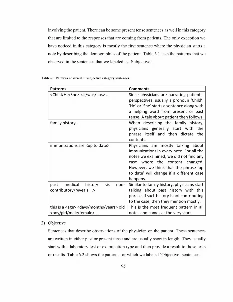
95

involving the patient. There can be some present tense sentences as well in this category

that are limited to the responses that are coming from patients. The only exception we

have noticed in this category is mostly the first sentence where the physician starts a

note by describing the demographics of the patient. Table 6.1 lists the patterns that we

observed in the sentences that we labeled as ‘Subjective’.

Table 6.1 Patterns observed in subjective category sentences

Patterns Comments

<Child/He/She> <is/was/has> ... Since physicians are narrating patients’ perspectives, usually a pronoun ‘Child’, ‘He’ or ‘She’ starts a sentence along with a helping word from present or past tense. A tale about patient then follows.

family history ... When describing the family history, physicians generally start with the phrase itself and then dictate the contents.

immunizations are <up to date> Physicians are mostly talking about immunizations in every note. For all the notes we examined, we did not find any case where the content changed. However, we think that the phrase ‘up to date’ will change if a different case happens.

past medical history <is non-contributory/reveals ...>

Similar to family history, physicians start talking about past history with this phrase. If such history is not contributing to the case, then they mention mostly.

this is a <age> <days/months/years> old <boy/girl/male/female> ...

This is the most frequent pattern in all notes and comes at the very start.

2) Objective

Sentences that describe observations of the physician on the patient. These sentences

are written in either past or present tense and are usually short in length. They usually

start with a laboratory test or examination type and then provide a result to those tests

or results. Table 6.2 shows the patterns for which we labeled ‘Objective’ sentences.

96

Table 6.2 Patterns observed in objective category sentences

Patterns Comments

<EXAM NAME> <is/was> <normal/unremarkable/uncomplicated/...>

Subjective sentences are talking about laboratory and physical exam results. Mostly these exams are good, so physicians are noting that down.

<EXAM NAME> reveals ... In case an exam reveals something, they also mention that.

On exam <child/he/she> <was/has> ... Mostly for physical exams, physicians simply use ‘On exam’.

the rest of exam <was/is> ... This pattern is also fairly visible in the notes.

<BODY PART> <is/are> <normal/clear/...> While defining results of physical exam, physicians note down the state of each body part they examined.

3) Assessment

Sentences that describe the assessment of the physician on the patient. These sentences

usually have the word ‘diagnosis’ in them along with a disease or medical condition.

Table 6.3 mentions some patters for ‘Assessment’ sentences

Table 6.3 Patterns observed in assessment category sentences

Patterns Comments

diagnosis is <DIAGNOSIS> The word ‘diagnosis’ is prominent in assessment category sentences.

<Medicine name and dosage> was prescribed

This is a loose pattern that we don’t find following a general style. In concept, this pattern mentions about the medications and treatments that are prescribed to the patient.

parents were <reassured/instructed> ... This pattern mentions all the instructions and reassurances that the physician has given to the parents of the patient which starts with the phrase ‘parents were instructed …’ and ‘parents were reassured that…’

97

4) Plan

Sentences that describe plans of the physician for the future treatments on the patient.

These sentences are usually written in the future tense. Table 6.4 lists the patterns for

‘Plan’ category sentences.

Table 6.4 Patterns observed in plan category sentences

Patterns Comments

... follow up ... This is a loose pattern that look for sentences with the phrase ‘follow up’. One variation that we observed multiple time is “Follow up as necessary”

<child/parents> <was/were> advised to return if...

This pattern mentions the advice of physician to return if some condition happens.

<Plans for future treatments> This is also a loose pattern. Generally, it looks for future treatment options. Physician does not seem to follow a strict word sequence for this.

All the sentences from our original dataset are extracted, and each sentence is manually

labeled according to the heuristics defined above. The labeled dataset is saved such that

features represent sentences and labels consist of one of the SOAP categories. In this

process, we observe that there is a class imbalance in our dataset. We note around 47%

Subjective, 35.3% Objective, 11% Assessment, and 6.7% Plan sentences in our dataset.

The imbalance property of our dataset matches the way clinical reports are usually written.

The same spread of classes is shown by Mowery [101] which also supports our observation.

98

6.2.2 Exemplar-based Concept Detection

Concept detection is a problem in NLP to extract relevant information from text

collections. Juckett presents an exemplar-based algorithm to link text to semantically

similar classes [102]. It maps each word within the text with probable class assignments.

Figure 6.1 highlights the algorithm. The algorithm is named Fuzzy matching. Juckett then

presents another algorithm Output array creation that takes the output values from Fuzzy

matching to create an array of detected concepts.

Figure 6.1 Exemplar based algorithms proposed by Juckett [102]

The Fuzzy matching algorithm expects to have some relevant text available that are already

categorized by human annotators to train exemplars. Exemplars are defined as the

collection of unique text strings that belong to specific semantic classes. In this algorithm,

exemplars are stored as Bag of Words (BOW) and Bag of Bi-characters (BOB). For each

sentence in the training set, an exemplar pair of BOW and BOB is created. BOW is the set

of all words within the training sentence. BOB is created after removing spaces from the

99

sentence and then extracting all overlapping character bi-grams. All generated exemplar

BOW and BOB are then stored along with the class assignments of training sentences.

To perform concept detection, the query sentence is first filtered for punctuations and

determiners are removed. It then creates overlapping word n-grams to the maximum of 5th

order (1-gram, 2-gram … 5-gram). Each word n-gram is converted into BOW and BOB

and stored. It gives a list of BOW and BOB for all possible word n-grams (till the order 5)

within the query. For each word n-gram, exemplars are selected that are of length between

n and 4n. For each selected exemplar, the Jaccard Index [120] of exemplar and word n-

gram is calculated for both; BOW and BOB, and the larger of these two values is selected.

After having similarity values of word n-gram with each exemplar, top n values are

selected. Word n-gram and exemplar information for the selected values are then stored.

Figure 6.2 Outline of word-class array [102]

After selecting the top n values, the algorithm Output array creation generates a word-by-

class map. Word-by-class map is a two-dimensional array where rows are the words in the

query text, and columns are the classes. Each cell within the array gets the score of word-

class combination. From the stored values in fuzzy matching, all values are selected whose

n-gram has the word, and exemplar belongs to the class. All these values are then added,

and the resultant value is stored as the word-class combination score. Figure 6.2 highlights

a word-class matrix as shown in [102].

100

6.2.3 Exemplar-based Sentence Classification

The second objective of this thesis requires the classification of textual units from

transcriptions into one of the SOAP categories. We consider sentences as a textual unit. To

achieve our objective, we develop an exemplar-based sentence classification algorithm on

the principles of exemplar-based concept detection by extending it to work on whole

sentences and provide confidence scores for each class. We use this algorithm due to its

nature to exploit word sequences. Moreover, since this algorithm work on exemplars, class

imbalance does not make a huge impact. As it selects top n scores for each n-gram, it can

optimally perform as long as there is a minimum of n exemplars available for each class.

Juckett took many assumptions during the development of the concept-detection algorithm

[102]. Since we adapt and extend this algorithm for a different problem and situation, we

identify four key areas that possibly develop an issue. Therefore, we investigate each of

those areas to find an optimal solution. After having a solution, we consider each area as

an independent variable to test the impact of our solution concerning the original

implementation. Details for each identified area are given below.

1) Stop Words

Stop words removal is a widely accepted and effective pre-processing step in various

problems of NLP [121]. However, the concept detection algorithm does not remove

stop words from their processing step. Moreover, in the arguments, Juckett [102] does

not provide any justification for keeping the stop words. Therefore, in this work, we

consider the removal of stop words since it has shown to have significant performance

improvements in text categorization tasks [122]. We apply a step to remove stop words

and make it optional in our classification algorithm by including it as an input

parameter.

2) Maximum word n-gram length limit

In the concept-detection algorithm, the query sentence converts into word-grams of

varying lengths from 1-gram to the maximum of 5-grams. There were two reasons

given for limiting the maximum n-gram length till the 5th order. Frist is that the dataset

101

on which Juckett [102] experimented, had shorter exemplars where 2/3rd of exemplars

were of word length five or less. The second reason is that each increasing word-gram

length increases the computation time exponentially. In our situation, the dataset has

sentences with an average length of 13 words, whereas 2/3rd of sentences are about 17

words or lower. With the same reasoning, we should look at 17-gram exemplars.

However, since the magnitude of the difference is more than double, a limit of 17-

grams can cause the algorithm to run for much more extended periods. Therefore, we

approach not to limit the length of maximum word n-grams in the algorithm; instead,

move the limit as an input parameter. There are two reasons for this approach. First, it

is easier to evaluate with varying maximum lengths. Second, this enables adaptation of

this algorithm to use on a dataset having sentences of different average lengths.

3) Exemplar type

The concept detection algorithm keeps full-text strings in the exemplars. Juckett [102]

does not report the considerations they took while defining exemplars. As we extend

the algorithm in our problem domain, we recognize that keeping full-text strings in

exemplars can cause some problems.

The current approach creates one exemplar per text string from the training text. We

have a small dataset, in which sentence length ranges from 3 words to 49 words. These

text strings come from natural speech and can have larger compound sentences.

Creating one exemplar for these larger text strings limits the opportunity to create

multiple exemplars. Moreover, due to the longer size of such text strings, they will be

skipped in many comparisons with shorter word n-grams, as the algorithm only selects

exemplars of length n to 4n for comparison with any word n-gram.

Size Sentence

A 5 Past medical history is unremarkable

B 5 Immunizations are up to date

C 11 Past medical history shows immunizations are up to date and unremarkable

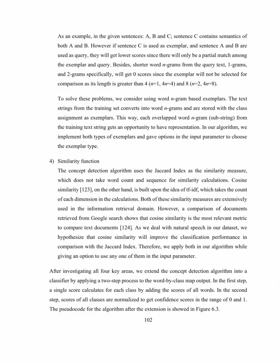
102

As an example, in the given sentences: A, B and C; sentence C contains semantics of

both A and B. However if sentence C is used as exemplar, and sentence A and B are

used as query, they will get lower scores since there will only be a partial match among

the exemplar and query. Besides, shorter word n-grams from the query text, 1-grams,

and 2-grams specifically, will get 0 scores since the exemplar will not be selected for

comparison as its length is greater than 4 (n=1, 4n=4) and 8 (n=2, 4n=8).

To solve these problems, we consider using word n-gram based exemplars. The text

strings from the training set converts into word n-grams and are stored with the class

assignment as exemplars. This way, each overlapped word n-gram (sub-string) from

the training text string gets an opportunity to have representation. In our algorithm, we

implement both types of exemplars and gave options in the input parameter to choose

the exemplar type.

4) Similarity function

The concept detection algorithm uses the Jaccard Index as the similarity measure,

which does not take word count and sequence for similarity calculations. Cosine

similarity [123], on the other hand, is built upon the idea of tf-idf, which takes the count

of each dimension in the calculations. Both of these similarity measures are extensively

used in the information retrieval domain. However, a comparison of documents

retrieved from Google search shows that cosine similarity is the most relevant metric

to compare text documents [124]. As we deal with natural speech in our dataset, we

hypothesize that cosine similarity will improve the classification performance in

comparison with the Jaccard Index. Therefore, we apply both in our algorithm while

giving an option to use any one of them in the input parameter.

After investigating all four key areas, we extend the concept detection algorithm into a

classifier by applying a two-step process to the word-by-class map output. In the first step,

a single score calculates for each class by adding the scores of all words. In the second

step, scores of all classes are normalized to get confidence scores in the range of 0 and 1.

The pseudocode for the algorithm after the extension is showed in Figure 6.3.

103

Figure 6.3 Pseudocode for Exemplar-based Sentence Classification Algorithm

104

6.2.4 Summary

To achieve our objective, we extend the exemplar-based concept detection algorithm for

SOAP classification. Five changes are done in this regard. The first change is to give an

option in the input parameter to remove stop words. Second, maximum word n-gram length

is made variable by taking a max length as input. Third, a word n-gram based exemplar is

developed, and an option is given as an input parameter to select the exemplar type. Fourth,

an option is given as an input parameter for similarity matric to use either the Jaccard Index

or Cosine Similarity. Fifth, the word-by-class map output is processed using a two-step

process to calculate a single confidence score for each class for the query.

105

6.3 Evaluation

6.3.1 Experimental Setup

We implemented our exemplar-based sentence classifier and then evaluated it on our

dataset using four independent variables that correspond to the four proposed

improvements. These variables are directly derived from the key areas that we identified

and enhanced. One of the independent variables is the maximum word n-gram length limit,

for which we did not specify any length; therefore, we experimented with lengths from 1

to 15. All other independent variables have two conditions each that give us 8 cases for

experiments. All these cases are given a number. Table 6.5 shows all the cases. Each of

these cases is experimented with varying maximum word n-gram length limits, which gave

us 120 total conditions to experiment (8 cases x 15 maximum word n-gram length limits).

Table 6.5 Cases based on Stop Word, Similarity Function and Exemplar type

Cases Stop Word Similarity Function Exemplar Type

1

w/ Stop Words

Cosine Sentence

2 n-gram

3 Jaccard

Sentence

4 n-gram

5

w/o Stop Words

Cosine Sentence

6 n-gram

7 Jaccard

Sentence

8 n-gram

For each condition, experiments are done in a one-vs-rest method, which means for each

SOAP category, a different binary classifier is trained and tested. For instance, when

experimenting with the ‘Subjective’ category, all subjective sentences in the dataset are

given positive labels (1), and all other sentences are given a negative label (0). The same

is repeated for all other categories. Although our classifier can perform multi-class

classification, yet we choose this strategy because SOAP categories have a very thin line

of separation which can impact the classification performance with our imbalanced dataset.

As an example, the sentence “we prescribed him ...” should be an assessment, whereas,

with a subtle change “we will prescribe him …” becomes a plan. However, in our dataset,

106

both of these categories have limited sentences. We also observe Mowery [101] applying

the same evaluation strategy, due to the same problems.

We conducted all experiments with 5x5 cross-validations. Dataset was randomly shuffled,

and 5-fold cross-validation was performed. This process was repeated four more times. For

each SOAP category, 25 results were retrieved, which in total gave us 100 results for each

condition. Ground truth, confidence score, and condition details were stored from all

experiments.

Confidence scores from our classifier show the predicted probability of having a positive

label. In this work, we did not specify any mechanism to select any threshold for binary

prediction (positive or negative). Therefore, to evaluate our classifier and to compare all

the experimental conditions, we used Precision-Recall Curve (PRC), since it provides an

accurate evaluation in case of imbalance dataset as compared to Receiver Operating

Characteristic (ROC) [125].

Area Under PRC (AUPRC) is represented by Average Precision (AP), where higher AP

means better classification performance. In this work, we used AP as the main

performance evaluation measure, which also serves as the dependent variable for all our

independent variables. We used regression testing to analyze the impact of each

independent variable, and based on the results, we selected the most optimal combination

of independent variables. We then thoroughly analyze the classification performance of the

experimental condition that is according to the selected variables. Three of our independent

variables: stop words, similarity function, and exemplar type; are categorical, though has

only two values in each. Therefore, we converted them into numerical variables for

regression testing.

We analyzed results from all SOAP categories separately as well as in combination. To

analyze the overall performance, we took both averages: micro-average and macro-

average. In micro-averaging, we directly calculate precision and recall values from overall

107

results, whereas, in macro-averaging, we calculated precision and recall values first for

individual categories and then averaged them.

Table 6.6 Conversion of categorical variables to numeric

Independent Variable Categorical Value Numeric Value

Maximum word n-gram Length Limit - 1 … 15

Stop Words w/ Stop Words 0

w/o Stop Words 1

Similarity Function Cosine 0

Jaccard 1

Exemplar Type Sentence 0

n-gram 1

In this evaluation, we focus on six main questions.

1. What is the baseline performance of the classifier before improvements?

2. What is the optimal maximum word n-gram length limit for SOAP classification?

3. Does the removal of stop words enhance classification performance?

4. What is the best exemplar type for SOAP classification?

5. What is the best similarity function for SOAP classification?

6. What is the performance of the classifier using optimal conditions?

6.3.2 Results

We experimented with all 120 conditions and analyzed the results to answer the six

questions. In this section, we first analyze the baseline performance of the classifier before

applying any improvement. Then we analyze the impact of each improvement on the

classification performance and select the optimal values for each improvement category.

Finally, we analyze the performance of the classifier on the conditions that correspond to

the optimal values.

108

• BASELINE PERFORMANCE

We consider case 3 using a maximum word n-gram length limit of 5 as the baseline

condition, as this condition equals of classifier without having any improvements. In this

condition, we observed an overall micro-averaged AP score of 0.886, while having AP

scores of 0.932 for ‘Subjective’, 0.911 for ‘Objective’, 0.563 for ‘Assessment’ and 0.765

for ‘Plan’ category. Figure 6.4 shows the AUPRC for the baseline condition.

Figure 6.4 Precision-Recall curve of the baseline condition

We compiled a list of example sentences along with their confidence scores from baseline

condition and actual SOAP category in Table 6.7. We highlight the top confidence scores

while underlined scores show that the highest confidence score is given to the actual SOAP

category. The list shows 3 examples each from the ‘Subjective’ and ‘Objective’ category,

and 2 examples each from ‘Assessment’ and ‘Plan’ categories.

109

Table 6.7 Confidence scores of sentences from the baseline condition

Sentence Confidence Scores Actual

SOAP Category

Subjective Objective Assessment Plan

1

paragraph past medical history immunizations are up to date

0.88791 0.0884 0.04866 0.05589 Subjective

2

immunizations up to date and no significant medical issues

0.83285 0.14976 0.11717 0.11628 Subjective

3

child was already starting to show return to normal function with crying and purposeful movements

0.46867 0.47539 0.41664 0.35019 Subjective

4

ear nose and throat exam revealed a runny nose mildly red throat and normal ears

0.17412 0.8412 0.11327 0.13244 Objective

5

new paragraph family sorry physical exam revealed entirely normal neurological exam with no focal findings

0.29106 0.69507 0.13999 0.14118 Objective

6

blood work was taken four hours after ingestion revealing non toxic acetaminophen levels

0.59756 0.23034 0.41212 0.14035 Objective

7 a diagnosis was croup treatment

0.3143 0.30527 0.71247 0.18112 Assessment

8 i note no allergies 0.66861 0.32717 0.19232 0.07669 Assessment

9 child will follow up with family doctor

0.23159 0.17391 0.12547 0.74356 Plan

10

a throat swab was sent today should it be positive we will call her and start her on antibiotics

0.3523 0.46499 0.41026 0.3531 Plan

110

• ANALYZING THE IMPACT OF IMPROVEMENTS

In all experimented conditions, the overall best performance was achieved by the condition

using case 1 with maximum word n-gram length limit of 5th order. This condition achieved

the highest micro-averaged AP score of 0.897. However, we observed that for individual

SOAP categories, different conditions showed better performance for different categories,

and no one condition was optimal for all SOAP categories. We list down the highest and

lowest AP scores we observed for each SOAP category along with overall combined scores

in Table 6.8. The magnitude of different highlights that our suggested improvements are

having a major impact on performance, especially with assessment and plan categories.

Table 6.8 Highest and Lowest AP scores for SOAP categories

SOAP Category Highest AP Lowest AP Difference

Subjective 0.957 0.881 0.076

Objective 0.919 0.836 0.083

Assessment 0.626 0.396 0.230

Plan 0.820 0.705 0.115

Micro-Averaged 0.897 0.812 0.085

Macro-Averaged 0.808 0.716 0.092

Results from regression tests on all 120 conditions showed that all independent variables

influenced classification performance, except similarity function which is consistently

insignificant for all SOAP categories. Table 6.9 highlights the results of regression testing.

Table 6.9 Summary of regression analysis results

Independent

Variables → Max n-gram Length Stop Words

Similarity

Function Exemplar Type

SOAP Categories ↓ P-value T Stat P-value T Stat P-value T Stat P-value T Stat

Subjective 1.125E-08 6.155 1.554E-19 -10.944 0.512 0.658 0.0725 -1.812

Objective 2.988E-07 5.444 3.503E-10 -6.869 0.189 1.321 2.920E-27 -14.292

Assessment 0.046 -2.019 1.036E-21 -11.874 0.375 -0.891 0.011 -2.584

Plan 0.009 -2.625 0.002 3.215 0.068 -1.841 0.039 -2.090

Micro-Average 3.375E-06 4.885 2.783E-32 -16.585 0.284 1.077 2.596E-11 -7.386

Macro-Average 0.984 -0.020 3.292E-22 -12.087 0.256 -1.141 2.490E-09 -6.469

111

• IMPACT OF MAXIMUM N-GRAM LENGTH LIMIT

Regression analysis showed that changing the maximum n-gram length limit had a

significant change in performance. However, the direction of change varied within SOAP

categories. We observed that sentences from ‘Subjective’ and ‘Objective’ categories were

better classified with higher order of n-grams, whereas, ‘Assessment’ and ‘Plan’ categories

favored shorter n-grams. Figure 6.5 draws the trend line of 6th-degree polynomial after

plotting all AP scores for all cases on ordinate with max n-gram lengths on the abscissa.

Figure 6.5 All AP scores over n-gram max length

112

The trend line validates the regression analysis; however, it highlights diminishing

increment in AP for ‘Subjective’ and ‘Objective’ categories with the increasing n-gram

lengths. For the ‘Assessment’ category, we see continuous declination of performance

along n-gram lengths. ‘Plan’ category, however, shows inconsistency, where performance

rapidly increased for the first few increments in n-gram lengths, then it started to fall,

nevertheless, the fall was not much. These opposite behaviors from SOAP categories

regarding max n-gram length explain the high P-value (0.984) for macro-averaged scores.

All 8 cases mostly followed the same trend; however, we did observe some anomalies. In

the ‘Subjective’ category, we marked 3 cases to have slight differences. In cases 3 and 8,

we saw another spike in scores with the higher values of max n-gram length. In case 5

specifically, we observed that n-gram lengths had no significant impact. We had the same

observation about the ‘Objective’ category in case 5. For the ‘Assessment’ category, cases

5 and 6 seemed to have no impact due to n-gram lengths, and case 8 was observed to be

favoring larger n-grams. We observed the same behavior with the ‘Plan’ category, where

cases 5 and 8 had no impact, whereas, case 6 favored larger n-grams. Overall, case 5

(without stop words, cosine similarity, sentence exemplars) appeared to be immune to the

n-gram lengths. We confirmed this observation by applying a t-test on the AP scores which

gave us a P-value of 0.196. After analyzing scores, we realized that there cannot be a single

selection for max n-gram length; therefore, we picked the best performing max n-gram

length from each case (Table 6.10).

Table 6.10 Best performing values for maximum n-gram length for each case

SOAP Categories ↓ All Cases Case 1 Case 2 Case 3 Case 4 Case 5 Case 6 Case 7 Case 8

Subjective 8 8 9 14 6 11 9 14 15

Objective 11 11 5 11 7 6 7 12 12

Assessment 1 1 3 1 2 15 15 1 15

Plan 6 2 3 2 2 14 8 6 8

Micro-Average 5 5 5 14 7 15 9 10 15

Macro-Average 3 3 3 6 2 15 15 6 15

113

• IMPACT OF STOP WORDS REMOVAL

It is evident from the regression analysis that stop words removal had a significant change

in the classification performance for all categories. However, for all the categories except

‘Plan’, the direction of change is negative (-ve t-stat value). This means that the

performance of only the ‘Plan’ category increased by removing stop words, whereas, all

other categories performed better when we keep stop-words in the sentences. Figure 6.6

shows the box plots for AP scores after categorizing them with and without stop words.

In Figure 6.6, all box plots are placed in the same sequence as shown in the legends on the

left. To be specific, from left to right, the first 2 plots represents the results from all SOAP

categories combined, the second pair represents results only for ‘Subjective’ category, the

third pair represents ‘Objective’ category, the fourth pair represent ‘Assessment’ category

and the fifth pair represent ‘Plan’ category. All the blue shaded plots (left on each pair) are

made from performance scores when stop words were kept in the sentences. On the other

hand, green-shaded plots (right on each pair) are from the scores when stop words were

removed. The x mark within plots shows the mean, and the dots outside plots show outliers.

While analyzing these plots, we can see that although ‘Plan’ sentences were better

classified without stop words, this performance was not very reliable, since the plot spread

is wider along with some outliers.

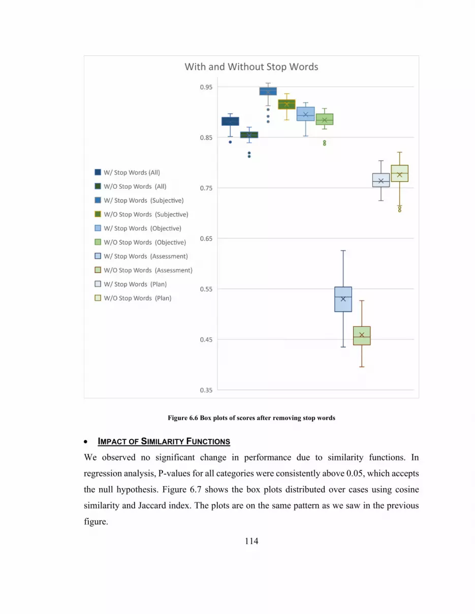
114

Figure 6.6 Box plots of scores after removing stop words

• IMPACT OF SIMILARITY FUNCTIONS

We observed no significant change in performance due to similarity functions. In

regression analysis, P-values for all categories were consistently above 0.05, which accepts

the null hypothesis. Figure 6.7 shows the box plots distributed over cases using cosine

similarity and Jaccard index. The plots are on the same pattern as we saw in the previous

figure.

115

Figure 6.7 Comparing performance based on similarity function (Cosine vs Jaccard)

• IMPACT OF EXEMPLAR TYPES

In our analysis, sentence based exemplars were better than n-gram based exemplars on all

SOAP categories. Figure 6.8 shows the box plots for scores based on exemplar-type. Blue

shaded plots are for sentence based exemplars and green shaded plots are for n-gram

exemplars. These plots validate the results of regression analysis as the mean and median

for each blue shaded plot is higher than the corresponding green-shaded plot.

116

Figure 6.8 Comparing performance based on exemplar type (sentence vs n-gram)

• OPTIMAL PERFORMANCE

Results from regression analysis presented that classification performance varied across

individual SOAP categories. Therefore, we inspected the optimal performance for each

category separately. We select the conditions having the highest AP scores for each

category and analyze the improvements that go within that condition. We also calculate the

F1 scores for the selected conditions using varying threshold levels. The highest F1 scores

are reported with each category. Table 6.11 provides a summary of optimal conditions for

117

each SOAP category along with the magnitude of improvement as compared to baseline

performance.

Table 6.11 Summary of optimal conditions for each SOAP category

SOAP Category

Base AP Score

Max AP Score

AP Improved

Optimal Maximum word n-gram length limit

Best Case

Subjective 0.932 0.957 0.025 8 1

Objective 0.911 0.919 0.008 11 3

Assessment 0.563 0.626 0.063 1 1

Plan 0.765 0.82 0.55 6 7

For the ‘Subjective’ category, we achieved max performance (AP: 0.957) with case 1 using

the maximum word n-gram length limit of the 8th order. This means that when our classifier

is set to break query sentences in word n-grams till 8-grams, use sentence based exemplar

and keep stop words, it will give the best classify ‘Subjective’ category sentences. Since

the similarity function has no significance, we select the condition with cosine similarity

as its score was moderately better. Figure 6.9 shows the AUPRC for this condition, where

we achieved an F1 score of 0.912.

Figure 6.9 Precision-Recall Curve of best performing condition for Subjective

118

We selected some examples and list them in Table 6.12 showing sentences with their actual

SOAP category and confidence scores we obtained using our classifiers with this condition.

The top 6 example shows the behavior of this condition on ‘Subjective’ sentences, while

rest shows behavior on other categories. We highlight the top-scoring category while

underline shows that our classifier predicted the actual category for the given sentence.

Table 6.12 Confidence scores of sentences from case 1 using 8-gram limit

Sentence Confidence Scores Actual SOAP

Category Subjective Objective Assessment Plan

1 no concussive findings

0.80509 0.296 0.25021 0 Subjective

2

immediately afterwards paramedics were called on arrival

0.4717 0.3464 0.50901 0.23972 Subjective

3 no medications 0.75963 0.24037 0.211 0 Subjective

4

past medical history reveals a healthy athletic male with no significant medical issues

0.75253 0.25061 0.22631 0.17429 Subjective

5

by the time she arrived at the IWK emergency she was awake and alert and cranky

0.51804 0.41937 0.33357 0.38002 Subjective

6

family history reveals febrile seizures in dad as a child

0.51926 0.40717 0.30884 0.38605 Subjective

7 tracheal palpation did not elicit pain

0.76971 0.39352 0.15284 0.24594 Objective

8 lungs were clear 0.18333 0.77103 0.24431 0.19585 Objective

9 the likely choice of antibiotics will be amoxicillin

0.36357 0.37519 0.42211 0.57157 Plan

10 diagnosis fracture radius ulna

0 0.55951 0.60422 0 Assessment

119

For the ‘Objective’ category, best scores (AP: 0.919) were achieved by condition using

case 3 and the maximum word n-gram length limit of 11. We achieved an F1 score of 0.846

in this condition. Figure 6.10 illustrates the AUPRC for this condition. Table 6.13 mentions

some examples from this condition, where the top 5 examples show the behavior of this

condition over the ‘Objective’ category. The rest of the examples show the performance

over other SOAP categories.

Table 6.13 Confidence scores of sentences from case 3 using 11-gram limit

Sentence Confidence Scores Actual

SOAP Category

Subjective Objective Assessment Plan

1

ear nose and throat exam revealed a red throat with no exudate suggestive of a viral pharyngitis

0.27987 0.72597 0.18146 0.1777 Objective

2

blood work was taken four hours after ingestion revealing non toxic acetaminophen levels

0.62871 0.20222 0.37966 0.14458 Objective

3 rest of the physical exam was without comment

0.20491 0.83209 0.15358 0.24458 Objective

4

new paragraph family sorry physical exam revealed entirely normal neurological exam with no focal findings

0.28433 0.71114 0.12414 0.12644 Objective

5

his neurovascular status in the effected limb is normal

0 0.67539 0 0 Objective

6

past medical history reveals immunizations up to date and normal

0.76841 0.22902 0.15446 0.13135 Subjective

120

birth and pregnancy history with no specialist and no regular medications and no known allergies

7 diagnosis fracture radius ulna

0 0.49184 0.69675 0 Assessment

8 chest xray revealed a dense left lower consolidation

0.34847 0.69141 0.21597 0.11372 Assessment

9 child will follow up with family doctor

0.29484 0.15295 0.0951 0.7286 Plan

10 parents were counseled and reassured

0.35712 0.33844 0.61333 0.29793 Plan

Figure 6.10 Precision-Recall Curve of best performing condition for Objective

121

For the ‘Assessment’ category, case 1 using maximum word n-gram length limit of 1st

order excelled (AP: 0.626) among all other conditions. This condition managed an F1 score

of 0.63. Figure 6.11 depicts AUPRC for this condition. Table 6.14 lists example sentences

from this condition showing highlighted confidence scores along with the actual SOAP

category. Top 5 examples show the behavior of this condition over ‘Assessment’ category

sentences, while rest show the behavior over other categories.

Table 6.14 Confidence scores of sentences from case 1 using 1-gram limit

Sentence Confidence Scores Actual SOAP

Category Subjective Objective Assessment Plan

1 a diagnosis was croup treatment

0.39702 0.299 0.71162 0.18063 Assessment

2 diagnosis is viral respiratory tract infection

0.41961 0.33547 0.64259 0.10616 Assessment

3 croup instructions were delivered

0.41324 0.5422 0.54945 0.33527 Assessment

4 i note no allergies 0.65644 0.35877 0.31561 0.14695 Assessment

5

diagnosis viral upper respiratory tract infection with febrile seizure

0.44084 0.31599 0.52301 0.18636 Assessment

6

immediately afterwards paramedics were called on arrival

0.4717 0.3464 0.50901 0.23972 Subjective

7

new paragraph impression is that this is simple febrile seizure

0.49094 0.33401 0.5078 0.33077 Objective

8

post reduction film showed good placement of the bones

0.5516 0.49871 0.49488 0.31146 Objective

9 child was hydrated and happy

0.44425 0.55868 0.4596 0.40219 Objective

10 parents were counseled and reassured

0.40641 0.38024 0.54527 0.38648 Plan

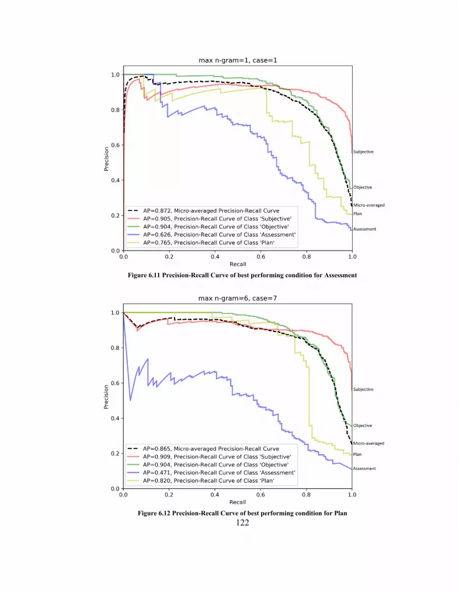
122

Figure 6.11 Precision-Recall Curve of best performing condition for Assessment

Figure 6.12 Precision-Recall Curve of best performing condition for Plan

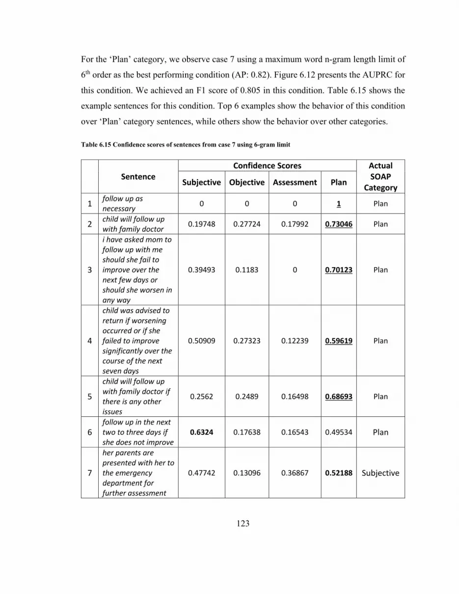
123

For the ‘Plan’ category, we observe case 7 using a maximum word n-gram length limit of

6th order as the best performing condition (AP: 0.82). Figure 6.12 presents the AUPRC for

this condition. We achieved an F1 score of 0.805 in this condition. Table 6.15 shows the

example sentences for this condition. Top 6 examples show the behavior of this condition

over ‘Plan’ category sentences, while others show the behavior over other categories.

Table 6.15 Confidence scores of sentences from case 7 using 6-gram limit

Sentence Confidence Scores Actual

SOAP Category

Subjective Objective Assessment Plan

1 follow up as necessary

0 0 0 1 Plan

2 child will follow up with family doctor

0.19748 0.27724 0.17992 0.73046 Plan

3

i have asked mom to follow up with me should she fail to improve over the next few days or should she worsen in any way

0.39493 0.1183 0 0.70123 Plan

4

child was advised to return if worsening occurred or if she failed to improve significantly over the course of the next seven days

0.50909 0.27323 0.12239 0.59619 Plan

5

child will follow up with family doctor if there is any other issues

0.2562 0.2489 0.16498 0.68693 Plan

6 follow up in the next two to three days if she does not improve

0.6324 0.17638 0.16543 0.49534 Plan

7

her parents are presented with her to the emergency department for further assessment

0.47742 0.13096 0.36867 0.52188 Subjective

124

8

child was already starting to show return to normal function with crying and purposeful movements

0.5657 0.35864 0.31614 0.47694 Subjective

9

she presented to a walk in clinic where she was told that she did not have a concussion

0.53009 0.36812 0.36995 0.54721 Subjective

10

instructions were given with regards to the delivery of ibuprofen as needed for pain and fever but the parents were cautioned that this would not reduce the risk of further seizures

0.43787 0.35454 0.3649 0.44165 Objective

6.4 Discussion

In this evaluation, we used 238 sentences to evaluate our classifier, which is far less than

4130 sentences that Mowery [101] used in their study; however, we achieved comparable

performance in almost all SOAP categories.

The performance of our classifier significantly improved with ‘Plan’ category sentences

when we applied the stop word removal operation. We observe that this change is

specifically due to the nature of ‘Plan’ sentences. Usually, in this category, physicians talk

in the future tense. For example, “Child will follow up …” and “We will perform …”. In

this case, when stop words are removed, the grammatical structure of a sentence becomes

more prominent and highlights those keywords like ‘will’ and ‘shall’ that be the key

identifiers of the future tense.

In our experiments, we also noticed a significant performance change with varying

maximum n-gram lengths, which ranged from the lowest overall AP score of 0.81 to the

highest of 0.89. We also observed that each SOAP category behaves differently with

125

different n-grams. Juckett [102] has implemented the concept-detection algorithm with the

max n-gram length equals to 5 for each class, owing to the small-phrase lengths of their

dataset. Using the same principle, we expected better performance with longer n-grams.

In this work, we also evaluated the use of the Jaccard index as the similarity function in

comparison to the cosine similarity function. We argued that the Jaccard Index only takes

the union of all lexicons for calculations and does not impact with repeated words, and

cosine similarity should work better. However, after experiments, our argument failed to

achieve support from the results, which made it evident that similarity function has no

significant impact on the performance.

6.5 Conclusion

This chapter provides an approach to use an exemplar-based concept detection algorithm

to develop a SOAP classifier. This classifier was implemented and was experimented with

four independent variables having a total of 120 variations where each variation was tested

for each of the SOAP categories separately. These experiments were defined to show a

directional insight into our approach, yet due to the small dataset, it does not provide a

meaningful conclusion. With the provided dataset, we make two suggestions. The first

suggestion is to use the longer n-grams for better classification in ‘Subjective’ and

‘Objective’ categories, whereas shorter n-grams for ‘Assessment’ and ‘Plan’ categories.

However, the drawback of longer n-grams is that for each increasing n-gram, processing

time increases exponentially. The second suggestion is to make separate classifiers for each

of the SOAP categories and remove stop words specifically for Plan category classifiers.

126

Chapter 7. DISCUSSION

7.1 Introduction

This chapter constructs a thorough discussion based on our work for both of our research

objectives. It highlights the observations that we made while performing this research. This

chapter then presents a 3-Layer solution framework that is based upon our observations.

Afterward, it reports the limitations of this work and provides possible and potential

improvements that can be done in the future. Finally, this chapter ends by providing a

conclusion towards this thesis.

7.2 Observations

We demonstrated our work on a 2-layer solution model, with the approach of having an

end-to-end solution. However, when we observe the output of the first layer, we found no

punctuation marks. The reason for this is that SR returns speech in free text format. These

texts bare no lexical entities other than words, such as punctuation marks, paragraph

indentation. On the other hand, Natural Language Processing (NLP) tasks usually work on

text data that are rich with punctuation marks. It means that output from SR systems can

create havoc with NLP methods; therefore, it is highly desired to enrich SR output with

punctuation marks before transmitting it to our final layer.

While working with the dictations, we also observed that some of them were recorded

while patients were still in the room. For our experiments, this created issues because of

the increased level of background noise. As we are working towards an end-to-end

solution, we made a realization that an autonomous report generation solution will allow

providers to record dictations anywhere and anytime. Most of the time, it should be

happening right after the encounter, possibly in front of the patient. For such scenarios, we

believe that patients will be hearing of what is said, hence they will get the chance to

provide clarification for any detail, which will be beneficial in reducing the dictation errors.

Fratzke [51] observed the same pattern when they implemented a voice-assisted

technology.

127

7.3 3-Layer Solution Framework

In this thesis, we observed that the output from the first layer is not fully compatible to be

used as the input of our second layer. Therefore, to develop a true end-to-end solution, we

need to specify a processing layer in between both layers whose purpose should be to

streamline the output of the first layer for the next layer.

Sentence boundaries are marked by using a dot, also known as period. This dot shows

where a sentence has ended in the text. In our final layer, we are using the sentence as the

unit to classify. Therefore, those transcriptions without punctuation marks will certainly

have some issues. A quick review shows that there are various solutions available that deal

with the punctuation prediction task. We found a punctuation predictor based on a

bidirectional recurrent neural network model with attention mechanism [126] that provides

pre-trained models based on Wikipedia text. We tested this solution on our dataset and

analyzed the results visually. We observed a few mistakes, though it generally felt

satisfactory. This simple review of the problem shown us that punctuation prediction is an

established problem in the research domain; hence we should give it a separate focus in

our solution.

Figure 7.1 Design for 3-Layer Solution Framework

With all the observations we made in this work, we present a potential 3-layer solution

framework for the problem of clinical documentation. All of the layers in this framework

are connected as a pipeline. Figure 7.1 represents the design of the 3-layer solution

framework. Each layer of this framework is defined below.

128

1. The first layer of this framework expects physicians recorded audio clips. This layer

processes the input audio into text by using a noise and domain robust speech

recognition system.

2. In the second layer, the transcriptions from the first layers are analyzed for

punctuations. Transcriptions are enriched with predicted punctuations and are given to

the third layer.

3. In the third layer, punctuated transcriptions are then classified for clinical reports.

Sentences from transcriptions are extracted and then classified for various categories

of the report structure.

7.4 Limitations

The size of the dataset possesses the biggest limitation of this work. Due to the small size

of the dataset, we had to tweak our experiments accordingly. While experimenting with

acoustic models, we initially wanted to train standalone models as well to hold a

comparison. However, a few trials with training exhibited the limitations. Therefore, we

skipped that scenario from our experiments. Similarly, during the SOAP classification, we

sensed a lower level of overall classification performance. The algorithm that we extended

and implemented in this layer was tested on a dataset five times in size than ours. Hence,

we believe that a lower dataset has introduced a limitation in our work.

Another limitation of this work is that all of the dataset labeling tasks were done by us,

without the help of any domain specialist. We perceived the need for a specialist at two

points. Firstly, at the time of generating gold standard transcriptions for dictation audios,

and secondly, when we labeled the sentences into SOAP categories. While preparing

transcriptions, we took help from one of the fellow members of our research group, who

has a medical degree. However, we do not consider this fellow a domain specialist since it

never practiced in the domain.

129

7.5 Future Work

This work is primarily experimental; however, it sets a direction for further research. This

thesis presents the solutions in terms of research areas that combine to form a solution

framework. Particularly, the solution depends on three research areas: continuous speech

recognition, punctuation prediction, and sentence classification. Any work that is done in

any of these research areas has the potential to enhance the presented solution framework.

Open-sourced offline SR are improving at a rapid pace. While working on this thesis, a

new open-sourced offline SR Wav2Letter++ [94] was released reporting better

performance then DeepSpeech [76] using similar models and datasets. Wav2Letter++ is

developed to scale and work in real-life environments. At the time of our experimentations,

its pre-trained models were not released, however, they are available at the time of writing

this thesis. Wav2Letter++ is also based on the concept of end-to-end SR, whilst providing

features to use custom acoustic models of different architectures. Therefore, we consider

that using this toolkit can be a perfect next step towards the enhancement of this work.

At the time of selecting methods for our final layer, we did not explore the sentence

classification solutions from other domains. One can argue this as a limitation, but we

consider this as the opportunity to move ahead in a logical manner. Since we were only

able to find one study that addressed the problem of sentence segmentation for SOAP

categories, the next logical step we took was to explore for similar problems within the

same (healthcare) domain. Therefore, we consider that this work provides the basis to

explore solution ideas from a different domain. We expect that examination of supervised

approaches towards text classification for this problem can pose as an appropriate work in

this direction.

In the previous subsections, this chapter presented a 3-layer solution framework. We

consider that this provides the opportunity to research the problem of clinical

documentation in a more systematic way. However, the framework still needs active

research and evaluations. Therefore, as future work, this 3-layer solution framework can

be enhanced.

130

7.6 Conclusion

Clinical documentation is a challenging process that poses multiple problems. Researchers

are experimenting with speech recognition since its inception to develop efficient solutions.

A review suggests that such solutions still lack adoption among healthcare providers. One

reason is the lack of accuracy in domain-specific noisy environments. Another reason is

that providers still need to intervene and perform manual changes. Therefore, this thesis

considers the problem from the end-to-end perspective. It identifies two research objectives

and translates them into individual layers of a solution model.

The first layer seeks efficient transcription of dictations in domain-specific and acoustically

distorted environments. We selected the DeepSpeech speech recognition system and

performed preliminary experiments. We then presented methods to enhance the

performance of both: acoustic and language; models. Evaluations show that all our

modeling methods improve DeepSpeech performance. We show that by adapting and fine-

tuning the pre-trained acoustic model, along with enhancing the pre-trained language

model using the augmented corpus from the domain-specific dataset, DeepSpeech can

achieve performance levels very close to Google Speech API.

The second layer aims to categorize transcriptions into SOAP categories. We select an

exemplar-based concept detection algorithm and extend it to develop a sentence classifier.

We identify four areas to enhance and implement our classifier for SOAP classification.

Evaluations show that each SOAP category requires a separate setting for optimal

performance, and no single set of independent variables will deliver the best performance

for all categories.

In this work, we observe that a two-layer solution could not exhibit as an end-to-end

solution due to the lack of punctuations in the transcriptions. Therefore, this thesis

discusses a 3-layered solution framework that can have the potential to become an end-to-

end solution.

131

REFERENCES

[1] T. K. Colicchio and J. J. Cimino, “Clinicians’ reasoning as reflected in electronic

clinical note-entry and reading/retrieval: a systematic review and qualitative

synthesis,” J. Am. Med. Informatics Assoc., vol. 26, no. 2, pp. 172–184, 2019.

[2] A. Mathioudakis, I. Rousalova, A. A. Gagnat, N. Saad, and G. Hardavella, “How to

keep good clinical records,” Breathe, vol. 12, no. 4, pp. 371–375, Dec. 2016.

[3] B. G. Arndt et al., “Tethered to the EHR: Primary care physician workload

assessment using EHR event log data and time-motion observations,” Ann. Fam.

Med., vol. 15, no. 5, pp. 419–426, 2017.

[4] C. Sinsky et al., “Allocation of physician time in ambulatory practice: A time and

motion study in 4 specialties,” Ann. Intern. Med., vol. 165, no. 11, pp. 753–760,

Dec. 2016.

[5] J. Holbrook and R. Aghababian, “A computerized audit of 15,009 emergency

department records,” Ann. Emerg. Med., vol. 19, no. 2, pp. 139–144, 1990.

[6] T. G. Poder, J. F. Fisette, and V. Déry, “Speech Recognition for Medical Dictation:

Overview in Quebec and Systematic Review,” J. Med. Syst., vol. 42, no. 5, p. 89,

May 2018.

[7] “mozilla/DeepSpeech: A TensorFlow implementation of Baidu’s DeepSpeech

architecture.” [Online]. Available: https://github.com/mozilla/DeepSpeech.

[Accessed: 20-Nov-2019].

[8] M. Amatayakul, “EHR versus EMR: what’s in a name?,” J. Healthc. Financ.

Manag. Assoc., vol. 63, no. 3, p. 24, 2009.

[9] W. Kondro, “CMAJ 2011 election survey: research.,” CMAJ, vol. 183, no. 8, pp.

E463--4, May 2011.

132

[10] J. H. Seo et al., “A pilot study on the evaluation of medical student documentation:

assessment of SOAP notes,” Korean J. Med. Educ., vol. 28, no. 2, pp. 237–241, Jun.

2016.

[11] M. Gardiner, “Clinical documentation.,” Texas dental journal, 2013. [Online].

Available: https://searchhealthit.techtarget.com/definition/clinical-documentation-

healthcare.

[12] D. R. Maines, Social Organization of Medical Work (Book)., vol. 8, no. 4. Chicago,

IL, US, IL, US: University of Chicago Press, 1986.

[13] K. R. Sando, E. Skoy, C. Bradley, J. Frenzel, J. Kirwin, and E. Urteaga, “Assessment

of SOAP note evaluation tools in colleges and schools of pharmacy,” Curr. Pharm.

Teach. Learn., vol. 9, no. 4, pp. 576–584, Jul. 2017.

[14] J. L. Belden, R. J. Koopman, S. J. Patil, N. J. Lowrance, G. F. Petroski, and J. B.

Smith, “Dynamic electronic health record note prototype: Seeing more by showing

less,” Journal of the American Board of Family Medicine, vol. 30, no. 6. American

Board of Family Medicine, pp. 691–700, 01-Nov-2017.

[15] M. R. Andrus et al., “Development and Validation of a Rubric to Evaluate Diabetes

SOAP Note Writing in APPE,” Am. J. Pharm. Educ., vol. 82, no. 9, p. 6725, 2018.

[16] L. A. Lenert, “Toward Medical Documentation That Enhances Situational

Awareness Learning,” AMIA ... Annu. Symp. proceedings. AMIA Symp., vol. 2016,

pp. 763–771, 2016.

[17] K. M. Lisenby et al., “Ambulatory care preceptors’ perceptions on SOAP note

writing in advanced pharmacy practice experiences (APPEs),” Curr. Pharm. Teach.

Learn., vol. 10, no. 12, pp. 1574–1578, Dec. 2018.

[18] P. F. Pearce, L. A. Ferguson, G. S. George, and C. A. Langford, “The essential

SOAP note in an EHR age,” Nurse Pract., vol. 41, no. 2, pp. 29–36, Feb. 2016.

133

[19] C. T. Lin, M. McKenzie, J. Pell, and L. Caplan, “Health care provider satisfaction

with a new electronic progress note format: SOAP vs APSO format,” JAMA Internal

Medicine, vol. 173, no. 2. American Medical Association, pp. 160–162, 28-Jan-

2013.

[20] E. L. Siegler and R. Adelman, “Copy and Paste: A Remediable Hazard of Electronic

Health Records,” American Journal of Medicine, vol. 122, no. 6, pp. 495–496, Jun-

2009.

[21] F. Jelinek, R. L. Mercer, and L. R. Bahl, “25 Continuous speech recognition:

Statistical methods,” in Handbook of Statistics, vol. 2, 1982, pp. 549–573.

[22] J. Li, L. Deng, Y. Gong, and R. Haeb-Umbach, “An overview of noise-robust

automatic speech recognition,” IEEE Trans. Audio, Speech Lang. Process., vol. 22,

no. 4, pp. 745–777, Apr. 2014.

[23] W. Ghai and N. Singh, “Literature Review on Automatic Speech Recognition,” Int.

J. Comput. Appl., vol. 41, no. 8, pp. 42–50, Mar. 2012.

[24] K. Jing and J. Xu, “A Survey on Neural Network Language Models.”

[25] A. J. Nathan and A. Scobell, “How China sees America,” Foreign Aff., vol. 91, no.

5, pp. 391–397, 2012.

[26] K. Saxena, R. Diamond, R. F. Conant, T. H. Mitchell, I. G. Gallopyn, and K. E.

Yakimow, “Provider Adoption of Speech Recognition and its Impact on

Satisfaction, Documentation Quality, Efficiency, and Cost in an Inpatient EHR.,”

AMIA Jt. Summits Transl. Sci. proceedings. AMIA Jt. Summits Transl. Sci., vol.

2017, pp. 186–195, 2018.

[27] F. R. Goss et al., “A clinician survey of using speech recognition for clinical

documentation in the electronic health record,” Int. J. Med. Inform., vol. 130, p.

103938, Oct. 2019.

134

[28] “Home - PubMed - NCBI.” [Online]. Available:

https://www.ncbi.nlm.nih.gov/pubmed/. [Accessed: 25-Nov-2019].

[29] L. Zhou et al., “Analysis of Errors in Dictated Clinical Documents Assisted by

Speech Recognition Software and Professional Transcriptionists,” JAMA Netw.

Open, vol. 1, no. 3, p. e180530, Jul. 2018.

[30] T. Hodgson, F. Magrabi, and E. Coiera, “Evaluating the efficiency and safety of

speech recognition within a commercial electronic health record system: A

replication study,” Appl. Clin. Inform., vol. 9, no. 2, pp. 326–335, 2018.

[31] B. W. Leeming, D. Porter, J. D. Jackson, H. L. Bleich, and M. Simon,

“Computerized radiologic reporting with voice data-entry,” Radiology, vol. 138, no.

5, pp. 585–588, Mar. 1981.

[32] A. H. Robbins et al., “Speech-controlled generation of radiology reports,”

Radiology, vol. 164, no. 2, pp. 569–573, Aug. 1987.

[33] A. Zafar, J. M. Overhage, and C. J. McDonald, “Continuous speech recognition for

clinicians,” J. Am. Med. Informatics Assoc., vol. 6, no. 3, pp. 195–204, 1999.

[34] M. M. Teel, R. Sokolowski, D. Rosenthal, and M. Belge, “Voice-enabled structured

medical reporting,” Conf. Hum. Factors Comput. Syst. - Proc., vol. 13, no. 1, pp.

595–602, 1998.

[35] K. Korn, “Voice recognition software for clinical use.,” J. Am. Acad. Nurse Pract.,

vol. 10, no. 11, pp. 515–517, 1998.

[36] R. Et, “Voice-enabled Reporting Systems Application of Information Technology,”

1997.

[37] O. A. Buch and N. P. Reddy, “Speaker verification for telemedical applications,”

Annu. Int. Conf. IEEE Eng. Med. Biol. - Proc., vol. 2, no. C, pp. 902–903, 1997.

135

[38] T. M. Murray, M. L. Kruse, J. A. Battcher, J. W. Woods, H. L. Edmonds, and M. P.

Palaheimo, “’Hands-off’--Voice activated automated anesthesia recordkeeping and

monitoring system (ARMS),” in Conference Proceedings - IEEE

SOUTHEASTCON, 1990, vol. 3, pp. 822–824.

[39] N. A. Linn, R. M. Rubenstein, A. E. Bowler, and J. L. Dixon, “Improving the quality

of emergency department documentation using the voice-activated word processor:

interim results.,” Proc. Annu. Symp. Comput. Appl. Med. Care, vol. 1992, no. 1, pp.

772–776, 1992.

[40] D. N. Mohr, D. W. Turner, G. R. Pond, J. S. Kamath, C. B. De Vos, and P. C.

Carpenter, “Speech recognition as a transcription aid: A randomized comparison

with standard transcription,” J. Am. Med. Informatics Assoc., vol. 10, no. 1, pp. 85–

93, 2003.

[41] Y. D. Derman, T. Arenovich, and J. Strauss, “Speech recognition software and

electronic psychiatric progress notes: Physicians’ ratings and preferences,” BMC

Med. Inform. Decis. Mak., vol. 10, no. 1, p. 44, Aug. 2010.

[42] G. C. David, A. C. Garcia, A. W. Rawls, and D. Chand, “Listening to what is said -

Transcribing what is heard: The impact of speech recognition technology (SRT) on

the practice of medical transcription (MT),” Sociol. Heal. Illn., vol. 31, no. 6, pp.

924–938, Sep. 2009.

[43] R. M. Issenman and I. H. Jaffer, “Use of voice recognition software in an outpatient

pediatric specialty practice,” Pediatrics, vol. 114, no. 3, pp. e290--e293, 2004.

[44] R. Hoyt and A. Yoshihashi, “Lessons learned from implementation of voice

recognition for documentation in the military electronic health record system.,”

Perspect. Health Inf. Manag., vol. 7, no. Winter, p. 1e, Jan. 2010.

[45] K. Patel and M. Harbord, “Digital dictation and voice transcription software

enhances outpatient clinic letter production: a crossover study,” Frontline

Gastroenterol., vol. 3, no. 3, pp. 162–165, Jul. 2012.

136

[46] T. Marukami, S. Tani, A. Matsuda, K. Takemoto, A. Shindo, and H. Inada, “A basic

study on application of voice recognition input to an electronic nursing record

system-evaluation of the function as an input interface,” J. Med. Syst., vol. 36, no.

3, pp. 1053–1058, Jun. 2012.

[47] M. Johnson et al., “A systematic review of speech recognition technology in health

care,” BMC Med. Inform. Decis. Mak., vol. 14, no. 1, p. 94, Dec. 2014.

[48] H. Suominen, L. Zhou, L. Hanlen, and G. Ferraro, “Benchmarking Clinical Speech

Recognition and Information Extraction: New Data, Methods, and Evaluations,”

JMIR Med. Informatics, vol. 3, no. 2, p. e19, Apr. 2015.

[49] S. Ajami, “Use of speech-to-text technology for documentation by healthcare

providers,” Natl. Med. J. India, vol. 29, no. 3, pp. 148–152, 2016.

[50] J. Fernandes, I. Brunton, G. Strudwick, S. Banik, and J. Strauss, “Physician

experience with speech recognition software in psychiatry: Usage and perspective,”

BMC Research Notes, vol. 11, no. 1. BioMed Central, p. 690, 01-Oct-2018.

[51] J. Fratzke, S. Tucker, H. Shedenhelm, J. Arnold, T. Belda, and M. Petera,

“Enhancing nursing practice by utilizing voice recognition for direct

documentation,” J. Nurs. Adm., vol. 44, no. 2, pp. 79–86, Feb. 2014.

[52] A. H. Abdelaziz, “Comparing Fusion Models for DNN-Based Audiovisual

Continuous Speech Recognition,” IEEE/ACM Trans. Audio Speech Lang. Process.,

vol. 26, no. 3, pp. 475–484, Mar. 2018.

[53] G. Saon, T. Sercu, S. Rennie, and H. K. J. Kuo, “The IBM 2016 English

conversational telephone speech recognition system,” in Proceedings of the Annual

Conference of the International Speech Communication Association,

INTERSPEECH, 2016, vol. 08-12-Sept, pp. 7–11.

137

[54] W. Xiong et al., “The microsoft 2016 conversational speech recognition system,”

ICASSP, IEEE Int. Conf. Acoust. Speech Signal Process. - Proc., pp. 5255–5259,

Sep. 2017.

[55] K. Garg and G. Jain, “A comparative study of noise reduction techniques for

automatic speech recognition systems,” in 2016 International Conference on

Advances in Computing, Communications and Informatics, ICACCI 2016, 2016, pp.

2098–2103.

[56] Y. Gong, “Speech recognition in noisy environments: A survey,” Speech Commun.,

vol. 16, no. 3, pp. 261–291, Apr. 1995.

[57] K. Kinoshita et al., “The reverb challenge: Acommon evaluation framework for

dereverberation and recognition of reverberant speech,” in IEEE Workshop on

Applications of Signal Processing to Audio and Acoustics, 2013, pp. 1–4.

[58] S. Thomas, S. Ganapathy, and H. Hermansky, “Recognition of reverberant speech

using frequency domain linear prediction,” IEEE Signal Process. Lett., vol. 15, pp.

681–684, 2008.

[59] A. Wisler, V. Berisha, A. Spanias, and J. Liss, “Noise robust dysarthric speech

classification using domain adaptation,” in 2016 Digital Media Industry and

Academic Forum, DMIAF 2016 - Proceedings, 2016, pp. 135–138.

[60] L. Deng et al., “Distributed speech processing in MiPad’s multimodal user

interface,” IEEE Trans. Speech Audio Process., vol. 10, no. 8, pp. 605–619, Nov.

2002.

[61] M. L. Seltzer, D. Yu, and Y. Wang, “An investigation of deep neural networks for

noise robust speech recognition,” in ICASSP, IEEE International Conference on

Acoustics, Speech and Signal Processing - Proceedings, 2013, pp. 7398–7402.

138

[62] H. Meutzner, S. Araki, M. Fujimoto, and T. Nakatani, “A generative-discriminative

hybrid approach to multi-channel noise reduction for robust automatic speech

recognition,” in ICASSP, IEEE International Conference on Acoustics, Speech and

Signal Processing - Proceedings, 2016, vol. 2016-May, pp. 5740–5744.

[63] T. Menne, R. Schluter, and H. Ney, “Speaker Adapted Beamforming for Multi-

Channel Automatic Speech Recognition,” 2018 IEEE Spok. Lang. Technol. Work.

SLT 2018 - Proc., pp. 535–541, Jun. 2019.

[64] S. F. Boll, “Suppression of Acoustic Noise in Speech Using Spectral Subtraction,”

IEEE Trans. Acoust., vol. 27, no. 2, pp. 113–120, Apr. 1979.

[65] J. S. Lim and A. V. Oppenheim, “Enhancement and Bandwidth Compression of

Noisy Speech,” Proc. IEEE, vol. 67, no. 12, pp. 1586–1604, 1979.

[66] R. Rehr and T. Gerkmann, “Cepstral noise subtraction for robust automatic speech

recognition,” in ICASSP, IEEE International Conference on Acoustics, Speech and

Signal Processing - Proceedings, 2015, vol. 2015-Augus, pp. 375–378.

[67] S. Park, Y. Jeong, M. S. Kim, and H. S. Kim, “Linear prediction-based

dereverberation with very deep convolutional neural networks for reverberant

speech recognition,” in International Conference on Electronics, Information and

Communication, ICEIC 2018, 2018, vol. 2018-Janua, no. 1, pp. 1–2.

[68] F. Weninger, S. Watanabe, Y. Tachioka, and B. Schuller, “Deep recurrent de-

noising auto-encoder and blind de-reverberation for reverberated speech

recognition,” in ICASSP, IEEE International Conference on Acoustics, Speech and

Signal Processing - Proceedings, 2014, no. 2, pp. 4623–4627.

[69] J. Li, Y. Huang, and Y. Gong, “Improved cepstra minimum-mean-square-error noise

reduction algorithm for robust speech recognition,” in ICASSP, IEEE International

Conference on Acoustics, Speech and Signal Processing - Proceedings, 2017, pp.

4865–4869.

139

[70] A. Narayanan and D. Wang, “Joint noise adaptive training for robust automatic

speech recognition,” in ICASSP, IEEE International Conference on Acoustics,

Speech and Signal Processing - Proceedings, 2014, pp. 2504–2508.

[71] A. Prodeus and K. Kukharicheva, “Training of automatic speech recognition system

on noised speech,” in 2016 IEEE 4th International Conference Methods and Systems

of Navigation and Motion Control, MSNMC 2016 - Proceedings, 2016, pp. 221–

223.

[72] J. Rajnoha, “Multi-Condition Training for Unknown Environment Adaptation in

Robust ASR Under Real Conditions,” Acta Polytech., vol. 49, no. 2, pp. 3–7, Jan.

2009.

[73] M. Fujimoto and H. Kawai, “Comparative evaluations of various factored deep

convolutional rnn architectures for noise robust speech recognition,” in ICASSP,

IEEE International Conference on Acoustics, Speech and Signal Processing -

Proceedings, 2018, vol. 2018-April, pp. 4829–4833.

[74] A. Prodeus and K. Kukharicheva, “Automatic speech recognition performance for

training on noised speech,” in 2nd International Conference on Advanced

Information and Communication Technologies, AICT 2017 - Proceedings, 2017, pp.

71–74.

[75] S. Watanabe et al., “ESPNet: End-to-end speech processing toolkit,” in Proceedings

of the Annual Conference of the International Speech Communication Association,

INTERSPEECH, 2018, vol. 2018-Septe, pp. 2207–2211.

[76] D. Amodei et al., “Deep speech 2: End-to-end speech recognition in English and

Mandarin,” 33rd Int. Conf. Mach. Learn. ICML 2016, vol. 1, pp. 312–321, Dec.

2016.

[77] A. Hannun et al., “Deep Speech: Scaling up end-to-end speech recognition,” Dec.

2014.

140

[78] D. Yu and J. Li, “Recent progresses in deep learning based acoustic models,”

IEEE/CAA J. Autom. Sin., vol. 4, no. 3, pp. 396–409, Jul. 2017.

[79] C. X. Qin, D. Qu, and L. H. Zhang, “Towards end-to-end speech recognition with

transfer learning,” Eurasip J. Audio, Speech, Music Process., vol. 2018, no. 1, p. 18,

Dec. 2018.

[80] Z. You, D. Su, and D. Yu, “Teach an All-rounder with Experts in Different

Domains,” in ICASSP, IEEE International Conference on Acoustics, Speech and

Signal Processing - Proceedings, 2019, vol. 2019-May, pp. 6425–6429.

[81] R. Lyer, M. Ostendorf, and H. Gish, “Using out-of-domain data to improve in-

domain language models,” IEEE Signal Process. Lett., vol. 4, no. 8, pp. 221–223,

Aug. 1997.

[82] D. Janiszek, R. De Mori, and F. Bechet, “Data augmentation and language model

adaptation,” in ICASSP, IEEE International Conference on Acoustics, Speech and

Signal Processing - Proceedings, 2001, vol. 1, pp. 549–552.

[83] M. Creutz, S. Virpioja, and A. Kovaleva, “Web augmentation of language models

for continuous speech recognition of SMS text messages,” in EACL 2009 - 12th

Conference of the European Chapter of the Association for Computational

Linguistics, Proceedings, 2009, pp. 157–165.

[84] H. Cucu, L. Besacier, C. Burileanu, and A. Buzo, “ASR domain adaptation methods

for low-resourced languages: Application to Romanian language,” in European

Signal Processing Conference, 2012, pp. 1648–1652.

[85] A. Sethy, S. Narayanan, and B. Ramabhadran, “Data Driven Approach for Language

Model Adaptation using Stepwise Relative Entropy Minimization,” in 2007 IEEE

International Conference on Acoustics, Speech and Signal Processing - ICASSP ’07,

2007, vol. 4, pp. IV-177-IV–180.

141

[86] A. K. Baughman, S. Hammer, and D. Provan, “Using language models for

improving speech recognition for U.S. Open Tennis Championships,” IBM J. Res.

Dev., vol. 61, no. 4/5, pp. 15:1-15:9, Jul. 2017.

[87] A. Graves and N. Jaitly, “Towards end-to-end speech recognition with recurrent

neural networks,” in 31st International Conference on Machine Learning, ICML

2014, 2014, vol. 5, pp. 3771–3779.

[88] J. J. Godfrey, E. C. Holliman, and J. McDaniel, “SWITCHBOARD: Telephone

speech corpus for research and development,” in ICASSP, IEEE International

Conference on Acoustics, Speech and Signal Processing - Proceedings, 1992, vol.

1, pp. 517–520.

[89] M. Schuster and K. K. Paliwal, “Bidirectional recurrent neural networks,” IEEE

Trans. Signal Process., vol. 45, no. 11, pp. 2673–2681, 1997.

[90] “TensorFlow.” [Online]. Available: https://www.tensorflow.org/. [Accessed: 05-

Nov-2019].

[91] Kenneth Heafield, “KenLM: Faster and Smaller Language Model Queries,” in

Proceedings of the Sixth Workshop on Statistical Machine Translation, 2011, pp.

187--197.

[92] D. Povey et al., “The Kaldi Speech Recognition Toolkit,” in IEEE 2011 Workshop

on Automatic Speech Recognition and Understanding, Hilton Waikoloa Village, Big

Island, Hawaii, US, Cambridge: IEEE Signal Processing Society, 2011.

[93] “PyTorch.” [Online]. Available: https://pytorch.org/. [Accessed: 05-Nov-2019].

[94] V. Pratap et al., “Wav2Letter++: A Fast Open-source Speech Recognition System,”

in ICASSP, IEEE International Conference on Acoustics, Speech and Signal

Processing - Proceedings, 2019, vol. 2019-May, pp. 6460–6464.

[95] A. Hannun, A. Lee, Q. Xu, and R. Collobert, “Sequence-to-Sequence Speech

Recognition with Time-Depth Separable Convolutions.”

142

[96] T. Likhomanenko, G. Synnaeve, and R. Collobert, “WHO NEEDS WORDS?

LEXICON-FREE SPEECH RECOGNITION A PREPRINT,” 2019.

[97] R. Singh, W. Walker, and P. Wolf, “The CMU Sphinx-4 Speech Recognition

System,” Evaluation, pp. 2–5.

[98] V. Këpuska, “Comparing Speech Recognition Systems (Microsoft API, Google API

And CMU Sphinx),” Int. J. Eng. Res. Appl., vol. 07, no. 03, pp. 20–24, Mar. 2017.

[99] A. Lee and T. Kawahara, “Recent development of open-source speech recognition

engine Julius,” APSIPA ASC 2009 - Asia-Pacific Signal Inf. Process. Assoc. 2009

Annu. Summit Conf., pp. 131–137, 2009.

[100] Google Cloud STT, “Cloud Speech-to-Text - Speech Recognition | Cloud Speech-

to-Text API | Google Cloud,” 2018. [Online]. Available:

https://cloud.google.com/speech-to-text/. [Accessed: 05-Nov-2019].

[101] D. Mowery, J. Wiebe, S. Visweswaran, H. Harkema, and W. W. Chapman,

“Building an automated SOAP classifier for emergency department reports,” J.

Biomed. Inform., vol. 45, no. 1, pp. 71–81, Feb. 2012.

[102] D. A. Juckett, E. P. Kasten, F. N. Davis, and M. Gostine, “Concept detection using

text exemplars aligned with a specialized ontology,” Data and Knowledge

Engineering, vol. 119, North-Holland, pp. 22–35, 01-Jan-2019.

[103] C. Cieri, D. Miller, and K. Walker, “The fisher corpus: A resource for the next

generations of speech-to-text,” in Proceedings of the 4th International Conference

on Language Resources and Evaluation, LREC 2004, 2004, pp. 69–71.

[104] V. Panayotov, G. Chen, D. Povey, and S. Khudanpur, “Librispeech: An ASR corpus

based on public domain audio books,” in ICASSP, IEEE International Conference

on Acoustics, Speech and Signal Processing - Proceedings, 2015, vol. 2015-Augus,

pp. 5206–5210.

143

[105] D. E. R. T. U. München and E. Gazetić, “Comparison Between Cloud-based and

Offline Speech Recognition Systems,” DER TECHNISCHEN UNIVERSITÄT

MÜNCHEN, 2018.

[106] A. R. Aronson and F. M. Lang, “An overview of MetaMap: Historical perspective

and recent advances,” J. Am. Med. Informatics Assoc., vol. 17, no. 3, pp. 229–236,

2010.

[107] “MeSH Browser.” [Online]. Available: http. [Accessed: 06-Nov-2019].

[108] “Deep Domain Adaptation In Computer Vision - Towards Data Science.” [Online].

Available: https://towardsdatascience.com/deep-domain-adaptation-in-computer-

vision-8da398d3167f. [Accessed: 16-Nov-2019].

[109] I. Redko, E. Morvant, A. Habrard, M. Sebban, and Y. Bennani, Advances in Domain

Adaptation Theory. ISTE Press - Elsevier, 2019.

[110] S. Ben-David, J. Blitzer, K. Crammer, A. Kulesza, F. Pereira, and J. W. Vaughan,

“A theory of learning from different domains,” Mach. Learn., vol. 79, no. 1–2, pp.

151–175, May 2010.

[111] M. Suzuki, N. Itoh, T. Nagano, G. Kurata, and S. Thomas, “Improvements to N-

gram Language Model Using Text Generated from Neural Language Model,” in

ICASSP, IEEE International Conference on Acoustics, Speech and Signal

Processing - Proceedings, 2019, vol. 2019-May, pp. 7245–7249.

[112] “These are the Easiest Data Augmentation Techniques in Natural Language

Processing you can think of — and they work.” [Online]. Available:

https://towardsdatascience.com/these-are-the-easiest-data-augmentation-

techniques-in-natural-language-processing-you-can-think-of-88e393fd610.

[Accessed: 13-Nov-2019].

144

[113] X. Zhang, J. Zhao, and Y. LeCun, “Character-level Convolutional Networks for

Text Classification,” Adv. Neural Inf. Process. Syst., vol. 2015-Janua, pp. 649–657,

Sep. 2015.

[114] “WordNet | A Lexical Database for English.” [Online]. Available:

https://wordnet.princeton.edu/. [Accessed: 18-Nov-2019].

[115] “Thesaurus.com | Synonyms and Antonyms of Words at Thesaurus.com.” [Online].

Available: https://www.thesaurus.com/. [Accessed: 18-Nov-2019].

[116] E. Abrahamsson, T. Forni, M. Skeppstedt, and M. Kvist, “Medical text

simplification using synonym replacement: Adapting assessment of word difficulty

to a compounding language.”

[117] S. Young Gunnar Evermann Mark Gales Thomas Hain Dan Kershaw Xunying Liu

Gareth Moore Julian Odell Dave Ollason Dan Povey Valtcho Valtchev Phil

Woodland, “The HTK Book,” 1995.

[118] “ARPA Language models – CMUSphinx Open Source Speech Recognition.”

[Online]. Available: https://cmusphinx.github.io/wiki/arpaformat/. [Accessed: 12-

Dec-2019].

[119] D. Klakow, “Log-linear interpolation of language models,” in ICSLP, 1998, no.

January, pp. 1–4.

[120] “Jaccard Index Definition | DeepAI.” [Online]. Available:

https://deepai.org/machine-learning-glossary-and-terms/jaccard-index. [Accessed:

19-Nov-2019].

[121] A. Schofield, M. Magnusson, and D. Mimno, “Pulling Out the Stops: Rethinking

Stopword Removal for Topic Models.”

[122] C. Silva and B. Ribeiro, “The Importance of Stop Word Removal on Recall Values

in Text Categorization,” in Proceedings of the International Joint Conference on

Neural Networks, 2003, vol. 3, pp. 1661–1666.

145

[123] G. Salton and M. J. McGill, Introduction to Modern Information Retrieval - Chapter

6, page 203. New York, NY, USA: McGraw-Hill, Inc., 1986.

[124] V. Thada and V. Jaglan, “Comparison of Jaccard, Dice, Cosine Similarity

Coefficient To Find Best Fitness Value for Web Retrieved Documents Using

Genetic Algorithm.”

[125] T. Saito and M. Rehmsmeier, “The precision-recall plot is more informative than

the ROC plot when evaluating binary classifiers on imbalanced datasets,” PLoS One,

vol. 10, no. 3, p. e0118432, Mar. 2015.

[126] O. Tilk and T. Alumäe, “Bidirectional recurrent neural network with attention

mechanism for punctuation restoration,” Proc. Annu. Conf. Int. Speech Commun.

Assoc. INTERSPEECH, vol. 08-12-Sept, no. September, pp. 3047–3051, 2016.

Appendix A. AP SCORES FOR SOAP CLASSIFICATION

Table A.1 Micro-Averaged AP-Scores of All Classes

Conditions

1 2 3 4 5 6 7 8

max

n-g

ram

len

gth

1 0.87152 0.84058 0.84252 0.85159 0.85459 0.81910 0.85184 0.81206

2 0.88061 0.86977 0.86825 0.87163 0.85796 0.84112 0.84968 0.84737

3 0.89237 0.86801 0.88100 0.87971 0.85346 0.84504 0.86390 0.85155

4 0.88720 0.87295 0.88759 0.87017 0.86087 0.85578 0.84566 0.84874

5 0.89675 0.88257 0.88595 0.87578 0.85288 0.83935 0.86702 0.86095

6 0.88218 0.87506 0.89358 0.87889 0.86509 0.84752 0.86476 0.84768

7 0.89209 0.87731 0.89252 0.88206 0.85856 0.85403 0.85644 0.85793

8 0.89512 0.87937 0.89425 0.88162 0.86106 0.85125 0.86177 0.84217

9 0.89086 0.88086 0.89328 0.87426 0.85684 0.85889 0.86656 0.85883

10 0.88856 0.88010 0.88967 0.87997 0.86259 0.84090 0.87013 0.85468

11 0.89134 0.87508 0.89125 0.87686 0.85885 0.85197 0.85369 0.84510

12 0.88846 0.87587 0.89400 0.88105 0.85362 0.84972 0.86796 0.85585

13 0.88870 0.86693 0.89375 0.87600 0.85575 0.83931 0.85644 0.85642

14 0.87369 0.87150 0.89542 0.87421 0.86041 0.85231 0.86727 0.84845

15 0.88625 0.87110 0.88969 0.87362 0.86681 0.85358 0.85403 0.86945

Table A.2 Macro-Averaged AP-Scores of All Classes

Conditions

1 2 3 4 5 6 7 8

max

n-g

ram

len

gth

1 0.79998 0.75426 0.76915 0.76028 0.76414 0.71638 0.77121 0.72274

2 0.80459 0.77561 0.79090 0.79243 0.75770 0.75826 0.76001 0.75260

3 0.80807 0.78539 0.79045 0.78538 0.76450 0.75281 0.76895 0.76315

4 0.79333 0.78249 0.78759 0.76358 0.76157 0.75335 0.75009 0.75843

5 0.80807 0.78237 0.79266 0.76794 0.75546 0.75181 0.75882 0.77015

6 0.78405 0.77931 0.80132 0.76689 0.76495 0.75031 0.77623 0.75212

7 0.79768 0.77712 0.79728 0.76820 0.76913 0.75521 0.74464 0.76786

8 0.79060 0.77587 0.79075 0.77641 0.76729 0.76235 0.76174 0.75969

9 0.79412 0.77728 0.78958 0.75259 0.76786 0.75242 0.74746 0.76732

10 0.78881 0.77820 0.78910 0.76923 0.76689 0.76032 0.76641 0.75721

11 0.79597 0.77398 0.79302 0.77094 0.76086 0.76354 0.76075 0.73879

12 0.78550 0.77857 0.79082 0.78332 0.74792 0.76637 0.76998 0.76448

13 0.79340 0.76907 0.79065 0.75373 0.75489 0.74406 0.75701 0.75932

14 0.77876 0.77184 0.79121 0.76499 0.76382 0.75211 0.75768 0.76184

15 0.78395 0.76465 0.78830 0.76070 0.77167 0.77614 0.74695 0.77150

147

Table A.3 AP-Scores of Two Classes (Subjective vs All)

Conditions

1 2 3 4 5 6 7 8 m

ax n

-gra

m le

ngt

h

1 0.90501 0.89149 0.88107 0.90806 0.91505 0.89741 0.89351 0.88440

2 0.93336 0.92283 0.91246 0.92152 0.92710 0.89072 0.88780 0.91804

3 0.94239 0.91865 0.92768 0.94003 0.90400 0.90593 0.91811 0.90613

4 0.94333 0.93144 0.94016 0.93299 0.92555 0.92370 0.90864 0.91680

5 0.95273 0.94288 0.93150 0.94842 0.92308 0.89751 0.92782 0.92390

6 0.94767 0.94021 0.94799 0.95153 0.92594 0.90369 0.90920 0.91275

7 0.94967 0.94131 0.94568 0.94773 0.90604 0.92381 0.92287 0.93336

8 0.95740 0.93798 0.94737 0.95101 0.92411 0.91136 0.90881 0.90886

9 0.94873 0.95107 0.94773 0.94274 0.90559 0.93126 0.92834 0.92388

10 0.94585 0.94358 0.94162 0.94536 0.92514 0.90118 0.93022 0.91742

11 0.94941 0.94000 0.93928 0.94745 0.92916 0.91121 0.90954 0.92416

12 0.95327 0.93872 0.94868 0.94808 0.91769 0.90859 0.92494 0.91523

13 0.95026 0.93438 0.95207 0.94390 0.92459 0.90395 0.90351 0.92396

14 0.93729 0.92832 0.95703 0.95128 0.91915 0.91917 0.93349 0.92274

15 0.95010 0.93111 0.94280 0.94444 0.92890 0.90565 0.91919 0.93660

Table A.4 AP-Scores of Two Classes (Objective vs All)

Conditions

1 2 3 4 5 6 7 8

max

n-g

ram

len

gth

1 0.90375 0.85260 0.87347 0.85891 0.87562 0.83632 0.87708 0.84159

2 0.89769 0.88483 0.89230 0.88298 0.88828 0.87137 0.88961 0.87662

3 0.90800 0.87393 0.90164 0.88555 0.89864 0.86943 0.88837 0.87976

4 0.90251 0.88142 0.90932 0.88496 0.89250 0.88372 0.88241 0.88566

5 0.90749 0.89293 0.91095 0.87892 0.87744 0.87557 0.90670 0.87394

6 0.89953 0.87594 0.91214 0.88282 0.90129 0.87362 0.90426 0.87490

7 0.90831 0.88341 0.90971 0.89423 0.89659 0.88469 0.88819 0.87681

8 0.91126 0.89258 0.91615 0.88261 0.88810 0.87390 0.89979 0.86681

9 0.91129 0.88297 0.91712 0.89106 0.90063 0.87826 0.90311 0.87514

10 0.91113 0.88707 0.91147 0.89191 0.89916 0.87251 0.90402 0.87803

11 0.91130 0.89220 0.91876 0.88074 0.88890 0.87459 0.90308 0.87257

12 0.90712 0.88976 0.91710 0.88228 0.89269 0.87452 0.90712 0.88933

13 0.90656 0.87141 0.91521 0.89360 0.89582 0.87049 0.90602 0.88417

14 0.90707 0.88522 0.91463 0.87518 0.89538 0.88458 0.90084 0.86635

15 0.90746 0.88614 0.91403 0.88204 0.89858 0.87836 0.88369 0.88256

148

Table A.5 AP-Scores of Two Classes (Assessment vs All)

Conditions

1 2 3 4 5 6 7 8 m

ax n

-gra

m le

ngt

h

1 0.62572 0.51981 0.58515 0.54963 0.48264 0.42715 0.50811 0.41564

2 0.58350 0.52195 0.56644 0.57512 0.43244 0.49223 0.47429 0.44123

3 0.59137 0.55334 0.55362 0.53872 0.44582 0.47400 0.47320 0.48630

4 0.53987 0.53424 0.54579 0.47043 0.43733 0.45967 0.40620 0.45350

5 0.60639 0.50124 0.56271 0.48171 0.43891 0.45345 0.42155 0.51026

6 0.51899 0.50746 0.56486 0.47294 0.43950 0.46482 0.47102 0.44875

7 0.55083 0.49840 0.57151 0.48657 0.48152 0.46541 0.42106 0.47560

8 0.53778 0.49373 0.55106 0.49727 0.45034 0.46598 0.46191 0.46540

9 0.55811 0.50911 0.53652 0.43471 0.45231 0.46446 0.44352 0.49112

10 0.55279 0.52788 0.53187 0.47275 0.43585 0.47011 0.46762 0.45519

11 0.56682 0.51310 0.55637 0.51224 0.43034 0.49273 0.44681 0.44773

12 0.54444 0.50459 0.54401 0.54557 0.43188 0.50355 0.44888 0.48709

13 0.56513 0.49285 0.53277 0.44201 0.39557 0.44036 0.45409 0.45822

14 0.52844 0.51922 0.53272 0.48407 0.42753 0.42670 0.42524 0.49405

15 0.54566 0.50524 0.53355 0.45283 0.49985 0.52671 0.44175 0.52557

Table A.6 AP-Scores of Two Classes (Plan vs All)

Conditions

1 2 3 4 5 6 7 8

max

n-g

ram

len

gth

1 0.76542 0.75312 0.73690 0.72453 0.78324 0.70465 0.80615 0.74932

2 0.80380 0.77281 0.79240 0.79008 0.78297 0.77872 0.78832 0.77451

3 0.79052 0.79562 0.77884 0.77720 0.80953 0.76187 0.79611 0.78040

4 0.78761 0.78287 0.75510 0.76593 0.79089 0.74632 0.80311 0.77775

5 0.76565 0.79241 0.76548 0.76269 0.78241 0.78070 0.77922 0.77251

6 0.77001 0.79364 0.78029 0.76025 0.79305 0.75910 0.82042 0.77209

7 0.78190 0.78535 0.76220 0.74425 0.79237 0.74693 0.74642 0.78567

8 0.75596 0.77918 0.74840 0.77476 0.80662 0.79814 0.77646 0.79768

9 0.75836 0.76597 0.75696 0.74186 0.81290 0.73569 0.71488 0.77912

10 0.74545 0.75426 0.77144 0.76691 0.80741 0.79749 0.76379 0.77821

11 0.75635 0.75062 0.75767 0.74334 0.79502 0.77564 0.78358 0.71071

12 0.73718 0.78119 0.75350 0.75734 0.74943 0.77882 0.79898 0.76625

13 0.75164 0.77764 0.76255 0.73542 0.80356 0.76144 0.76442 0.77093

14 0.74224 0.75461 0.76046 0.74943 0.81323 0.77798 0.77115 0.76423

15 0.73256 0.73611 0.76280 0.76349 0.75936 0.79384 0.74318 0.74126