hmms and related speech recognition technologies - CiteSeerX

Springer Handbook on Speech Processing and Speech Communication 1

HMMS AND RELATED SPEECH RECOGNITION TECHNOLOGIES

Steve Young

Cambridge University Engineering DepartmentTrumpington Street, Cambridge, CB2 1PZ, United Kingdom

e-mail: [email protected]

Almost all present day continuous speech recog-nition (CSR) systems are based on Hidden MarkovModels (HMMs). Although the fundamentals ofHMM-based CSR have been understood for severaldecades, there has been steady progress in refiningthe technology both in terms of reducing the impactof the inherent assumptions, and in adapting the mod-els for specific applications and environments. Theaim of this chapter is to review the core architectureof a HMM-based CSR system and then outline themajor areas of refinement incorporated into modern-day systems.

1. INTRODUCTION

Automatic continuous speech recognition (CSR) issufficiently mature that a variety of real world ap-plications are now possible including command andcontrol, dictation, transcription of recorded speechand interactive spoken dialogues. This chapter de-scribes the statistical models that underlie current-day systems: specifically, the hidden Markov model(HMM) and its related technologies.

The foundations of modern HMM-based contin-uous speech recognition technology were laid downin the 1970’s by groups at Carnegie-Mellon, IBMand Bell Labs [1, 2, 3]. Reflecting the compu-tational power of the time, initial development inthe 1980’s focussed on whole word small vocabu-lary applications[4, 5]. In the early 90’s, attentionswitched to continuous speaker-independent recog-nition. Starting with the artificial 1000 wordRe-source Managementtask [6], the technology devel-oped rapidly and by the mid-1990’s, reasonable ac-curacy was being achieved for unrestricted dictation.

Much of this development was driven by a seriesof DARPA and NSA programmes[7] which set evermore challenging tasks culminating most recently insystems for multilingual transcription of broadcastnews programmes[8] and for spontaneous telephoneconversations[9].

Although the basic framework for CSR has notchanged significantly in the last ten years, the de-tailed modelling techniques developed within thisframework have evolved to a state of considerablesophistication (e.g. [10, 11]). The result has beensteady and significant progress and it is the aim ofthis chapter to describe the main techniques by whichthis has been achieved. Many research groups havecontributed to this progress, and each will typicallyhave their own architectural perspective. For the sakeof logical coherence, the presentation given here issomewhat biassed towards the architecture developedat Cambridge and supported by the HTK SoftwareToolkit[12]1.

The chapter is organised as follows. In section 2,the core architecture of a typical HMM-based recog-niser is described [13]. Subsequent sections then de-scribe the various improvements which have beenmade to this core over recent years. Section 3 dis-cusses methods of HMM parameter estimation andissues relating to improved covariance modelling.In sections 4 and 5, methods of normalisation andadaptation are described which allow HMM-basedacoustic models to more accurately represent specificspeakers and environments. Finally in section 6, themulti-pass architecture refinements adopted by mod-ern transcription system is described. The chapterconcludes in section 7 with some general observa-

1Available for free download athtk.eng.cam.ac.uk


tions and conclusions.

2. ARCHITECTURE OF A HMM-BASEDRECOGNISER

The principal components of a large vocabulary con-tinuous speech recogniser are illustrated in Fig 1.The input audio waveform from a microphone is con-verted into a sequence of fixed size acoustic vectorsY = y1..yT in a process called feature extraction.The decoder then attempts to find the sequence ofwordsW = w1 . . . wK which is most likely to havegeneratedY , i.e. the decoder tries to find

W = argmaxW

{p(W |Y )} (1)

However, sincep(W |Y ) is difficult to model directly,Bayes’ Rule is used to transform (1) into the equiva-lent problem of finding:

W = argmaxW

{p(Y |W )p(W )}. (2)

The likelihoodp(Y |W ) is determined by anacous-tic modeland the priorp(W ) is determined by alan-guage model.2 The basic unit of sound representedby the acoustic model is thephone. For example, theword “bat” is composed of three phones /b/ /ae/ /t/.About 40 such phones are required for English.

For any givenW , the corresponding acousticmodel is synthesised by concatenating phone modelsto make words as defined by a pronunciation dictio-nary. The parameters of these phone models are esti-mated from training data consisting of speech wave-forms and their orthographic transcriptions. The lan-guage model is typically anN -gram model in whichthe probability of each word is conditioned only onits N − 1 predecessors. TheN -gram parameters areestimated by counting N-tuples in appropriate textcorpora. The decoder operates by searching throughall possible word sequences using pruning to re-move unlikely hypotheses thereby keeping the searchtractable. When the end of the utterance is reached,

2In practice, the acoustic model is not normalised and the lan-guage model is often scaled by an empirically determined constantand a word insertion penalty is added i.e. in the log domain the to-tal likelihood is calculated aslog p(Y |W ) + αp(W ) + β|W |whereα is typically in the range 8 to 20 andβ is typically in therange 0 to -20.

the most likely word sequence is output. Alterna-tively, modern decoders can generate lattices contain-ing a compact representation of the most likely hy-potheses.

The following sections describe these processesand components in more detail.

2.1. Feature Extraction

The feature extraction stage seeks to provide a com-pact encoding of the speech waveform. This encod-ing should minimise the information loss and providea good match with the distributional assumptionsmade by the acoustic models. Feature vectors aretypically computed every 10ms using an overlappinganalysis window of around 25ms. One of the sim-plest and most widely used encoding schemes usesMel-Frequency Cepstral Coefficients (MFCCs)[14].These are generated by applying a truncated cosinetransformation to a log spectral estimate computedby smoothing an FFT with around 20 frequency binsdistributed non-linearly across the speech spectrum.The non-linear frequency scale used is called aMelScaleand it approximates the response of the hu-man ear. The cosine transform is applied in orderto smooth the spectral estimate and decorrelate thefeature elements.

Further psychoacoustic constraints are incorpo-rated into a related encoding calledPerceptual LinearPrediction (PLP)[15]. PLP computes linear predic-tion coefficients from a perceptually weighted non-linearly compressed power spectrum and then trans-forms the linear prediction coefficients to cepstral co-efficients. In practice, PLP can give small improve-ments over MFCCs, especially in noisy environmentsand hence it is the preferred encoding for many sys-tems.

In addition to the spectral coefficients, first order(delta) and second-order (delta-delta) regression co-efficients are often appended in a heuristic attemptto compensate for the conditional independence as-sumption made by the HMM-based acoustic models.The final result is a feature vector whose dimension-ality is typically around 40 and which has been par-tially but not fully decorrelated.


2.2. HMM Acoustic Models

As noted above, the spoken words inW are decom-posed into a sequence of basic sounds calledbasephones. To allow for possible pronunciation varia-tion, the likelihoodp(Y |W ) can be computed overmultiple pronunciations3

p(Y |W ) =∑

Q

p(Y |Q)p(Q|W ) (3)

Each Q is a sequence of word pronunciationsQ1 . . .QK where each pronunciation is a sequenceof base phonesQk = q

(k)1 q

(k)2 . . .. Then

p(Q|W ) =

K∏

k=1

p(Qk|wk) (4)

wherep(Qk|wk) is the probability that wordwk ispronounced by base phone sequenceQk. In practice,there will only be a very small number of possibleQk for eachwk making the summation in (3) easilytractable.

Each base phoneq is represented by a continuousdensity hidden Markov model (HMM) of the formillustrated in Fig 2 with transition parameters{aij}and output observation distributions{bj()}. The lat-ter are typically mixtures of Gaussians

bj(y) =

M∑

m=1

cjmN (y; µjm, Σjm) (5)

whereN denotes a normal distribution with meanµjm and covarianceΣjm, and the number of compo-nentsM is typically in the range 10 to 20. Since thedimensionality of the acoustic vectorsy is relativelyhigh, the covariances are usually constrained to bediagonal. The entry and exit states arenon-emittingand they are included to simplify the process of con-catenating phone models to make words.

Given the composite HMMQ formed by con-catenating all of its constituent base phones then theacoustic likelihood is given by

p(Y |Q) =∑

X

p(X, Y |Q) (6)

3Recognizers often approximate this by amaxoperation so thatalternative pronunciations can be decoded as though they were al-ternative word hypotheses.

whereX = x(0)..x(T ) is a state sequence throughthe composite model and

p(X, Y |Q) = ax(0),x(1)

T∏

t=1

bx(t)(yt)ax(t),x(t+1)

(7)The acoustic model parameters{aij} and{bj()}

can be efficiently estimated from a corpus of trainingutterances using Expection-Maximisation (EM)[16].For each utterance, the sequence of baseforms isfound and the corresponding composite HMM con-structed. A forward-backward alignment is used tocompute state occupation probabilities (the E-step)and the means and covariances are then estimatedvia simple weighted averages (the M-step)[12, Ch7]. This iterative process can be initialised by as-signing the global mean and covariance of the data toall Gaussian components and setting all transititionprobabilities to be equal. This gives a so-calledflatstart model. The number of component Gaussians inany mixture can easily be increased by cloning, per-turbing the means and then re-estimating using EM.

This approach to acoustic modelling is often re-ferred to as thebeads-on-a-stringmodel, so-calledbecause all speech utterances are represented by con-catenating a sequence of phone models together.The major problem with this is that decomposingeach vocabulary word into a sequence of context-independent base phones fails to capture the verylarge degree of context-dependent variation that ex-ists in real speech. For example, the base form pro-nunciations for “mood” and “cool” would use thesame vowel for “oo”, yet in practice the realisationsof “oo” in the two contexts are very different due tothe influence of the preceding and following conso-nant. Context independent phone models are referredto asmonophones.

A simple way to mitigate this problem is to usea unique phone model for every possible pair of leftand right neighbours. The resulting models are calledtriphonesand if there areN base phones, there arelogically N3 potential triphones. To avoid the result-ing data sparsity problems, the complete set oflog-ical triphonesL can be mapped to a reduced set ofphysical modelsP by clustering and tying togetherthe parameters in each cluster. This mapping pro-cess is illustrated in Fig 3 and the parameter tyingis illustrated in Fig 4 where the notation x-q+y de-


notes the triphone corresponding to phone q spokenin the context of a preceding phone x and a followingphone y. The base phone pronunciations Q are de-rived by simple look-up from the pronunciation dic-tionary, these are then mapped to logical phones ac-cording to the context, finally the logical phones aremapped to physical models. Notice that the context-dependence spreads across word boundaries and thisis essential for capturing many important phonologi-cal processes. For example, the [p] in “stop that” hasits burst suppressed by the following consonant.

The clustering of logical to physical models typi-cally operates at the state-level rather than the modellevel since it is simpler and it allows a larger setof physical models to be robustly estimated. Thechoice of which states to tie is made using decisiontrees[17]. Each state position4 of each phoneq hasa binary tree associated with it. Each node of thetree carries a question regarding the context. To clus-ter statei of phoneq, all statesi of all of the log-ical models derived fromq are collected into a sin-gle pool at the root node of the tree. Depending onthe answer to the question at each node, the pool ofstates is successively split until all states have trick-led down to leaf nodes. All states in each leaf nodeare then tied to form a physical model. The ques-tions at each node are selected from a predeterminedset to maximize the likelihood of the training datagiven the final set of state-tyings. If the state outputdistributions are single component Gaussians and thestate occupation counts are known, then the increasein likelihood achieved by splitting the Gaussians atany node can be calculated simply from the countsand model parameters without reference to the train-ing data. Thus, the decision trees can be grown veryefficiently using a greedy iterative node splitting al-gorithm. Fig 5 illustrates this tree-based clustering.In the figure, the logical phones s-aw+n and t-aw+nwill both be assigned to leaf node 3 and hence theywill share the same central state of the representativephysical model.5

The partitioning of states using phonetically-driven decision trees has several advantages. In par-ticular, logical models which are required but werenot seen at all in the training data can be easily syn-

4invariably each phone model has three states5The total number of tied-states in a large vocabulary speaker

independent system typical ranges between 1000 and 5000 states

thesised. One disadvantage is that the partitioningcan be rather coarse. This problem can be reducedusing so-calledsoft-tying[18]. In this scheme, a post-processing stage groups each state with its one ortwo nearest neighbours and pools all of their Gaus-sians. Thus, the single Gaussian models are con-verted to mixture Gaussian models whilst holding thetotal number of Gaussians in the system constant.

To summarise, the core acoustic models of amodern speech recogniser is typically comprised ofa set of tied-state mixture Gaussian HMM-basedacoustic models. This core is commonly built in thefollowing steps[12, Ch 3]:

1. A flat-start monophone set is created in whicheach base phone is a monophone single-Gaussian HMM with means and covariancesequal to the mean and covariance of the trainingdata.

2. The parameters of the single-Gaussian mono-phones are iteratively re-estimated using 3 or 4iterations of EM.

3. Each single Gaussian monophone q is clonedonce for each distinct triphone x-q+y that ap-pears in the training data.

4. The set of training data single-Gaussian tri-phones is iteratively re-estimated using EM andthe state occupation counts of the last iterationare saved.

5. A decision tree is created for each state in eachbase phone, the single-Gaussian triphones aremapped into a smaller set of tied-state triphonesand iteratively re-estimated using EM.

6. Mixture components are iteratively split and re-estimated until performance peaks on a held-outdevelopment set.

The final result is the required tied-state context-dependent mixture Gaussian acoustic model set.


2.3. N -gram Language Models

The prior probability of a word sequenceW =w1..wK required in (2) is given by

p(W ) =

K∏

k=1

p(wk|wk−1, . . . , w1) (8)

For large vocabulary recognition, the conditioningword history in (8) is usually truncated toN − 1words to form anN -gram language model

p(W ) =

K∏

k=1

p(wk|wk−1, wk−2, . . . , wk−N+1) (9)

whereN is typically in the range 2 to 4. TheN -gram probabilities are estimated from training textsby countingN -gram occurrences to form maximumlikelihood (ML) parameter estimates. For example,let C(wk−2wk−1wk) represent the number of occur-rences of the three wordswk−2wk−1wk and similarlyfor C(wk−2wk−1), then

p(wk|wk−1, wk−2) ≈C(wk−2wk−1wk)

C(wk−2wk−1)(10)

The major problem with this simple ML estimationscheme is data sparsity. This can be mitigated by acombination of discounting and backing-off, knownasKatz smoothing[19]

p(wk|wk−1, wk−2)

=C(wk−2wk−1wk)

C(wk−2wk−1)if C > C′

= dC(wk−2wk−1wk)

C(wk−2wk−1)if 0 < C ≤ C′

= α(wk−1, wk−2) p(wk|wk−1) otherwise (11)

whereC′ is a count threshold,d is a discount coeffi-cient andα is a normalisation constant. Thus, whenthe N -gram count exceeds some threshold, the MLestimate is used. When the count is small the sameML estimate is used but discounted slightly. The dis-counted probability mass is then distributed to the un-seenN -grams which are approximated by a weightedversion of the corresponding bigram. This idea canbe applied recursively to estimate any sparseN -gramin terms of a set of back-off weights andN−1-grams.

The discounting coefficient is based on the Turing-Good estimated = (r +1)nr+1/rnr wherenr is thenumber ofN -grams that occur exactlyr times in thetraining data. Although Katz smoothing is effective,there are now known to be variations which work bet-ter. In particular, Kneser-Ney smoothing consistentlyoutperforms Katz on most tasks [20, 21].

An alternative approach to robust language modelestimation is to use class-based models in which forevery wordwk there is a corresponding classck [22,23]. Then,

p(W ) =

K∏

k=1

p(wk|ck)p(ck|ck−1, . . . , ck−N+1)

(12)As for word based models, the classN -gram proba-bilities are estimated using ML but since there are farfewer classes (typically a few hundred) data sparsityis much less of an issue. The classes themselves arechosen to optimise the likelihood of the training setassuming a bigram class model. It can be shown thatwhen a word is moved from one class to another, thechange in perplexity depends only on the counts of arelatively small number of bigrams. Hence, an itera-tive algorithm can be implemented which repeatedlyscans through the vocabulary, testing each word tosee if moving it to some other class would increasethe likelihood [24].

In practice it is found that for reasonably sizedtraining sets, an effective language model for largevocabulary applications consists of a word-based tri-gram or 4-gram interpolated with a class-based tri-gram.

2.4. Decoding and Lattice Generation

As noted in the introduction to this section, themost likely word sequenceW given a sequence offeature vectorsY = y1..yT is found by search-ing all possible state sequences arising from allpossible word sequences for the sequence whichwas most likely to have generated the observeddata Y . An efficient way to solve this problemis to use dynamic programming. Letφj(t) =maxX {p(y1, . . . ,yt, x(t) = j|M)} i.e. the maxi-mum probability of observing the partial sequencey1..yt and then being in statej at time t given themodelM. This probability can be efficiently com-


puted using the Viterbi algorithm

φj(t) = maxi

{φi(t − 1)aij} bj(yt) (13)

It is initialised by settingφj(t) to 1 for the ini-tial state and 0 for all other states. The probabil-ity of the most likely word sequence is then givenby maxj{φj(T )} and if every maximisation decisionis recorded, a traceback will yield the required bestmatching state/word sequence.

In practice, a direct implementation of the abovealgorithm becomes unmanageably complex for con-tinuous speech where the topology of the models, thelanguage model constraints and the need to boundthe computation must all be taken account of. For-tunately, much of this complexity can be abstractedaway by a simple change in viewpoint.

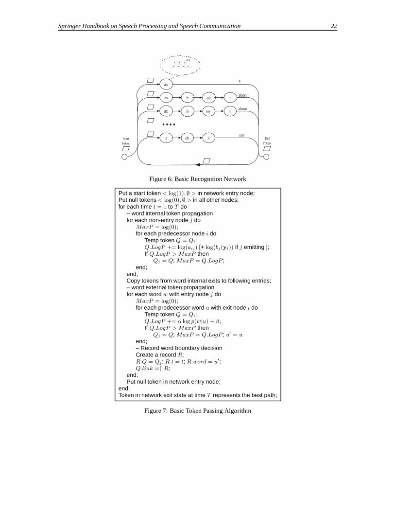
First, the HMM topology can be made explicitby constructing a recognition network. For task ori-ented applications, this network can represent the ut-terances that the user is allowed to say i.e. it can rep-resent a recognition grammar. For large vocabularyapplications, it will typically consist of all vocabu-lary words in parallel in a loop. In both cases, wordsare represented by a sequence of phone models as de-fined by the pronunciation dictionary (see Fig 6), andeach phone model consists of a sequence of states asindicated by the inset. If a word has several pronun-ciations as in the general case described by (3), theyare simply placed in parallel.

Given this network, at any timet in the search, asingle hypothesis consists of a path through the net-work representing an alignment of states with featurevectorsy1..yt, starting in the initial state and endingat statej, and having a log likelihoodlog φj(t). Thispath can be made explicit via the notion of atokenconsisting of a pair of values< logP, link > wherelogP is the log likelihood6 and link is a pointer toa record of history information [25]. Each networknode corresponding to each HMM state can store asingle token and recognition proceeds by propagat-ing these tokens around the network.

The basic Viterbi algorithm given above can nowbe recast for continuous speech recognition as theTo-ken Passingalgorithm shown in outline in Fig 7. Thetermnoderefers to a network node corresponding toa single HMM state. These nodes correspond to ei-

6Often referred to as thescore

ther entry states, emitting states or exit states. Es-sentially, tokens are passed from node to node and ateach transition the token score is updated.

When a token transitions from the exit of a wordto the start of the next word, its score is updatedby the language model probability plus any word in-sertion penalty. At the same time the transition isrecorded in a recordR containing a copy of the token,the current time and identity of the preceding word.The link field of the token is then updated to pointto the recordR. As each token proceeds through thenetwork it accumulates a chain of these records. Thebest token at timeT in a valid network exit node canthen be examined and traced back to recover the mostlikely word sequence and the boundary times.

The above Token Passing algorithm and associ-ated recognition network is an exact implementationof the dynamic programming principle embodied in(13). To convert this to a practical decoder for speechrecognition, the following steps are required:

1. For computational efficiency, only tokens whichhave some likelihood of being on the best pathshould be propagated. Thus, every propagationcycle, the log probability of the most likely to-ken is recorded. All tokens whose probabilitiesfall more than a constant below this are deleted.This results in a so-calledbeam searchand theconstant is called thebeam width.

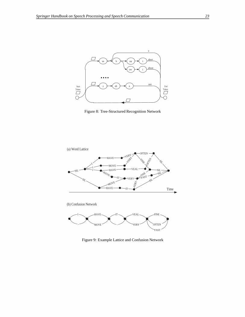
2. As a consequence of beam search, 90% of thecomputation is actually spent on the first twophones of every word, after that most of the to-kens fall outside of the beam and are pruned.To exploit this, the recognition network shouldbetree-structuredso that word initial phones areshared (see Fig 8).

3. However, sharing initial phones makes it impos-sible to apply an exact language model probabil-ity during word-external token propagation sincethe identity of the following word is not known.Simply delaying the application of the languagemodel until the end of the following word is notan option since that would make pruning inef-fective. Instead, an incremental approach mustbe adopted in which the language model proba-bility is taken to be the maximum possible prob-ability given the set of possible following words.As tokens move through the tree-structured word


graph, the set of possible next words reduces ateach phone transition and the language modelprobability can be updated with a more accurateestimate.

4. The HMMs linked into the recognition networkshould be context dependent and for best per-formance, this dependency should span wordboundaries. At first sight this requires a massiveexpansion of the network, but in fact a compactstatic network representation of cross-word tri-phones is possible [26].

5. The dynamic programming principle relies onthe principle that the optimal path at any nodecan be extended knowing only the state infor-mation given at that node. The use ofN -gramlanguage models causes a problem here sinceunique network nodes would be needed to distin-guish all possibleN − 1 word histories and forlarge vocabulary decoders this is not tractable.Thus, the algorithm given in Fig 7 will only workfor bigram language models. A simple way tosolve this problem is to store multiple tokens ineach state thereby allowing paths with differinghistories to “stay alive” in parallel. Token prop-agation now requires a merge and sort operationwhich although computationally expensive canbe made tractable.

The above description of a large vocabulary de-coder covers all of the essential elements needed torecognise continuous speech in real time using just asingle pass over the data. For off-line batch transcrip-tion of speech, significant improvements in accuracycan be achieved by performing multiple passes overthe data. To make this possible, the decoder mustbe capable of generating and saving multiple recog-nition hypotheses. A compact and efficient structurefor doing this is theword lattice[27, 28, 29].

A word lattice consists of a set of nodes repre-senting points in time and a set of spanning arcs rep-resenting word hypotheses. An example is shown inFig 9 part (a). In addition to the word ids shown inthe figure, each arc can also carry score informationsuch as the acoustic and language model scores. Lat-tices are generated via the mechanism for recordingword boundary information outlined in Fig 7, exceptthat instead of recording just the best token which isactually propagated to following word entry nodes,

all word-end tokens are recorded. For the simplesingle-token Viterbi scheme, the quality of latticesgenerated in this way will be poor because many ofthe close matching second best paths will have beenpruned by exercising the dynamic programming prin-ciple. The multiple token decoder does not sufferfrom this problem, especially if it is used with a rela-tively short-span bigram language model.

Lattices are extremely flexible. For example, theycan be rescored by using them as an input recognitionnetwork and they can be expanded to allow rescor-ing by a higher order language model. They canalso be compacted into a very efficient representationcalled aconfusion network[30, 31]. This is illustratedin Fig 9 part (b) where the “-” arc labels indicatenull transitions. In a confusion network, the nodesno longer correspond to discrete points in time, in-stead they simply enforce word sequence constraints.Thus, parallel arcs in the confusion network do notnecessarily correspond to the same acoustic segment.However, it is assumed that most of the time the over-lap is sufficient to enable parallel arcs to be regardedas competing hypotheses. A confusion network hasthe property that for every path through the originallattice, there exists a corresponding path through theconfusion network. Each arc in the confusion net-work carries the posterior probability of the corre-sponding wordw. This is computed by finding thelink probability of w in the lattice using a forward-backward procedure, summing over all occurrencesof w and then normalising so that all competing wordarcs in the confusion network sum to one. Confusionnetworks can be used for minimum word-error de-coding, to provide confidence scores and for mergingthe outputs of different decoders [32, 33, 34, 35] (seesection 6).

Finally, it should be noted that all of the aboverelates to one specific approach to decoding. If sim-ple Viterbi decoding was the only requirement, thenthere would be little variation amongst decoder im-plementations. However, the requirement to supportcross-word context-dependent acoustic models andlong span language models has led to a variety of de-sign strategies. For example, rather than have multi-ple tokens, the network state can be dynamically ex-panded to explicitly represent the currently hypoth-esised cross-word acoustic and long-span languagemodel contexts [36, 37]. These dynamic network


decoders are more flexible than static network de-coders, but they are harder to implement efficiently.Recent advances in weighted finite-state transducertechnology offer the possibility of integrating all ofthe required information (acoustic models, pronunci-ation, language model probabilities, etc) into a sin-gle very large but highly optimised network) [38].This approach offers both flexibility and efficiencyand is therefore extremely useful for both researchand practical applications.

A completely different approach to decoding isto avoid the breadth-first strategy altogether and use adepth-first strategy. This gives rise to a class of recog-nisers calledstack decoders. Stack decoders werepopular in the very early developments of ASR sincethey can be very efficient. However, they require dy-namic networks and their run-time search character-istcs can be difficult to control [39, 40].

3. HMM-BASED ACOUSTIC MODELLING

The key feature of the HMM-based speech recogni-tion architecture described in the preceding section isthe use of diagonal covariance multiple componentmixture Gaussians for modelling the spectral distri-butions of the speech feature vectors. If speech reallydid have the statistics assumed by these HMMs andif there was sufficient training data, then the mod-els estimated using maximum likelihood would beoptimal in the sense of minimum variance and zerobias [41]. However, since this is not the case, there isscope for improving performance both by using alter-native parameter estimation schemes and by improv-ing the models. In this section, both of these aspectsof HMM design will be discussed. Firstly, discrimi-native training is described and then methods of im-proved covariance modelling will be explored.

3.1. Discriminative Training

Standard maximum likelihood training attempts tofind a parameter setλ which maximises the log like-lihood of the training data, i.e. for training sentencesY 1 . . . Y R, the objective function is

FML (λ) =

R∑

r=1

log pλ(Y r|MWr) (14)

whereWr is the word sequence given by the tran-scription of ther’th training sentence andMWr

isthe corresponding composite HMM synthesised byconcatenating phone models (denoted byQ in sec-tion 2.2). This objective function can be maximisedstraightforwardly using a version of EM known asthe Baum-Welch algorithm [42]. This involves it-eratively finding the probability of state-componentoccupation for each frame of training data usinga forward-backward algorithm, and then computingweighted averages. For example, defining the fol-lowing “counts”

Θrjm(M) =

Tr∑

t=1

γrjm(t)yr

t

∣

∣

∣

∣

∣

M

(15)

and

Γrjm(M) =

Tr∑

t=1

γrjm(t)

∣

∣

∣

∣

∣

M

(16)

whereγrjm(t) is the probability of the model occu-

pying mixture componentm in statej at timet giventraining sentenceY r and modelM, then the updatedmean estimate is given by ML as

µjm =

∑R

r=1 Θrjm(MWr

)∑R

r=1 Γrjm(MWr

)(17)

i.e. the average of the sum of the data weighted bythe model component occupancy.

The key problem with the ML objective functionis that it simply fits the model to the training data andit takes no account of the model’s ability to discrim-inate. An alternative objective function is to max-imise the conditional likelihood using the MaximumMutual Information (MMI) criterion [41, 43]

FMMI (λ) =

R∑

r=1

logpλ(Y r|MWr

)p(Wr))∑

W pλ(Y r|MW )p(W ))

(18)Here the numerator is the likelihood of the data giventhe correct word sequenceWr whilst the denomina-tor is the total likelihood of the data given all possi-ble word sequencesW . Thus, the objective functionis maximised by making the correct model sequencelikely and all other model sequences unlikely. It istherefore discriminative. Note also that it incorpo-rates the effect of the language model and hence moreclosely represents recognition conditions.


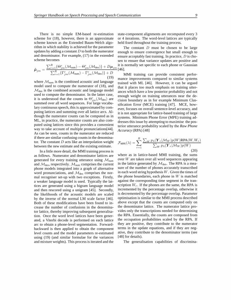
There is no simple EM-based re-estimationscheme for (18), however, there is an approximatescheme known as the Extended Baum-Welch algo-rithm in which stability is achieved for the parameterupdates by adding a constantD to both the numeratorand denominator. For example, (17) in the extendedscheme becomes

µjm =

∑R

r=1{Θrjm(Mnum) − Θr

jm(Mden)} + Dµjm∑R

r=1{Γrjm(Mnum) − Γr

jm(Mden)} + D(19)

whereMnum is the combined acoustic and languagemodel used to compute the numerator of (18), andMden is the combined acoustic and language modelused to compute the denominator. In the latter case,it is understood that the counts inΘr

jm(Mden) aresummed over all word sequences. For large vocabu-lary continuous speech, this is approximated by com-puting lattices and summing over all lattice arcs. Al-though the numerator counts can be computed as inML, in practice, the numerator counts are also com-puted using lattices since this provides a convenientway to take account of multiple pronunciations[44].As can be seen, counts in the numerator are reducedif there are similar confusing counts in the denomina-tor. The constantD acts like an interpolation weightbetween the new estimate and the existing estimate.

In a little more detail, the MMI training process isas follows. Numerator and denominator lattices aregenerated for every training utterance usingMnum

andMden, respectively.Mnum comprises the currentphone models integrated into a graph of alternativeword pronunciations, andMden comprises the nor-mal recogniser set-up with two exceptions. Firstly,a weaker language model is used. Typically the lat-tices are generated using a bigram language modeland then rescored using a unigram [45]. Secondly,the likelihoods of the acoustic models are scaledby the inverse of the normal LM scale factor [46].Both of these modifications have been found to in-crease the number of confusions in the denomina-tor lattice, thereby improving subsequent generalisa-tion. Once the word level lattices have been gener-ated, a Viterbi decode is performed on each latticearc to obtain a phone-level segmentation. Forward-backward is then applied to obtain the componentlevel counts and the model parameters re-estimatedusing (19) (and similar formulae for the variancesand mixture weights). This process is iterated and the

state-component alignments are recomputed every 3or 4 iterations. The word-level lattices are typicallyheld fixed throughout the training process.

The constantD must be chosen to be largeenough to ensure convergence but small enough toensure acceptably fast training. In practice,D is cho-sen to ensure that variance updates are positive andit is normally set specific to each phone or Gaussian[46].

MMI training can provide consistent perfor-mance improvements compared to similar systemstrained with ML [46]. However, it can be arguedthat it places too much emphasis on training utter-ances which have a low posterior probability and notenough weight on training utterances near the de-cision boundary as in for example Minimum Clas-sification Error (MCE) training [47]. MCE, how-ever, focuses on overall sentence-level accuracy, andit is not appropriate for lattice-based training of largesystems. Minimum Phone Error (MPE) training ad-dresses this issue by attempting to maximise the pos-terior utterance probability scaled by theRaw PhoneAccuracy(RPA) [48]

FMPE(λ) =R∑

r=1

∑

W pλ(Y r|MW )p(W )RPA(W, Wr)∑

W pλ(Y r|MW )p(W )

(20)where as in lattice-based MMI training, the sumsoverW are taken over all word sequences appearingin the lattice generated byMden. The RPA is a mea-sure of the number of phones accurately transcribedin each word string hypothesisW . Given the times ofthe phone boundaries, each phone inW is matchedagainst the corresponding time segment in the tran-scriptionWr. If the phones are the same, the RPA isincremented by the percentage overlap, otherwise itis decremented by the percentage overlap. Parameteroptimisation is similar to the MMI process describedabove except that the counts are computed only onthe denominator lattice. The numerator lattice pro-vides only the transcriptions needed for determiningthe RPA. Essentially, the counts are composed fromthe occupation probabilities scaled by the RPA. Ifthey are positive, they contribute to the numeratorterms in the update equations, and if they are neg-ative, they contribute to the denominator terms (see[48] for details).

The generalisation capabilities of discrimina-


tively trained systems can be improved by interpo-lating with ML. For example, the H-criterion inter-polates objective functions:αFMMI + (1 − α)FML

[49]. However, choosing an optimal value forα isdifficult and the effectiveness of the technique de-creases with increasing training data [50]. A moreeffective technique isI-smoothingwhich increasesthe weight of the numerator counts depending on theamount of data available for each Gaussian compo-nent [48]. This is done by scaling the numeratorcountsΓr

jm(Mnum) andΘrjm(Mnum) by

1 +τ

∑

r Γrjm(Mnum)

(21)

whereτ is a constant (typically about 50). Asτ in-creases from zero, more weight is given to ML.

3.2. Covariance Modelling

An alternative way of improving the acoustic mod-els is to allow them to more closely match the truedistribution of the data. The baseline acoustic mod-els outlined in section 2.2 use mixtures of diagonalcovariance Gaussians chosen as a compromise be-tween complexity and modelling accuracy. Never-theless, the data is clearly not diagonal and hencefinding some way of improving the covariance mod-elling is desirable. In general the use of full covari-ance Gaussians in large vocabulary systems would beimpractical due to the sheer size of the model set7.However, the use of shared orstructuredcovariancerepresentations allow covariance modelling to be im-proved with very little overhead in terms of memoryand computational load.

One the simplest and most effective structuredcovariance representations is the Semi-Tied Covari-ance (STC) matrix [51]. STC models the covarianceof them’th Gaussian component as

Σm = A−1Σm(A−1)T (22)

whereΣm is the component specific diagonal covari-ance andA is the STC matrix shared by all compo-nents. If the component meanµm = Aµm then com-ponent likelihoods can be computed by

N (y; µm, Σm) = |A|N (Ay; µm, Σm) (23)

7Although given enough data it can be done [11]

Hence, a single STC matrix can be viewed as a lineartransform applied in feature space. The componentparametersµm andΣm represent the means and vari-ances in the transformed space and can be estimatedin the normal way by simply transforming the train-ing data. The STC matrix itself can be efficiently esti-mated using a row by row iterative scheme. Further-more it is not necessary during training to store thefull covariance statistics at the component level. In-stead, an interleaved scheme can be used in which theA matrix statistics are updated on one pass throughthe training data, and then the component parame-ters are estimated on the next pass [51]8. This can beintegrated into themixing-upoperation described insection 2.2. For example, a typical training schememight start with a single Gaussian system and anidentity A matrix. The system is then iteratively re-fined by reestimating the component parameters, up-dating theA matrix, and mixing-up until the requirednumber of Gaussians per state is achieved. As well ashaving a single globalA matrix, the Gaussian com-ponents can be clustered and assigned oneA matrixper cluster. For example, there could be oneA ma-trix per phone or per state depending on the amountof training data available and the acceptable numberof parameters. Overall, the use of STC can be ex-pected to reduce word error rates by around 5% to10% compared to the baseline system. In addition toSTC, other types of structured covariance modellinginclude factor-analysed HMMs [52], sub-space con-strained precision and means (SPAM) [53], and EM-LLT [54].

It can be shown [51] that simultaneous opti-misation of the full set of STC parameters (i.e.{A, µm, Σm}) is equivalent to maximising the auxil-iary equation

QSTC =∑

t,m

γm(t) log

(

|A|2

|diag(A W (m)AT )|

)

(24)where

W (m) =

∑

t γm(t)ym(t)ym(t)T

∑

t γm(t)(25)

and whereym(t) = y(t) − µm. If each Gaus-sian component is regarded as a class, thenW (m) is

8The means can in fact be updated on both passes.


the within class covariance and it can be shown that(24) is the maximum likelihood solution to a gen-eralised form of linear discriminant analysis calledHeteroscedastic LDA (HLDA) in which class covari-ances are not constrained to be equal [55]. The matrixA can therefore be regarded as a feature space trans-form which discriminates Gaussian components andthis suggests a simple extension by whichA can alsoperform a subspace projection, i.e.

y = Ay =

[

A[p]y

A[d−p]y

]

=

[

y[p]

y[d−p]

]

(26)

where the d-dimensional feature space is divided intop usefuldimensions andd − p nuisancedimensions.The matrixA[p] projectsy into a p-dimensional sub-space which is modelled by the diagonal Gaussianmixture components of the acoustic models. Thed − p nuisance dimensions are modelled by a globalnon-discriminating Gaussian. Equation 24 can there-fore be factored as

QHLDA =∑

t,m

γm(t)

log

(

|A|2

|diag(A[p] W (m)AT[p])||diag(A[d−p] TAT

[d−p])|

)

(27)

whereT is the global covariance of the training data.The forms of equations (24) and (27) are similar andthe optimal value forA[p] can be estimated by thesame row-by-row iteration used in the STC case.

For application to LVCSR,y can be constructedeither by concatenating successive feature vectors, oras is common in HTK-based systems, the standard39-element feature vector comprised of static PLPcoefficients plus their 1st and 2nd derivatives are aug-mented by the 3rd derivatives and then projected backinto 39 dimensions using a39×52 HLDA transform.

Finally note that, as with semi-tied covariances,multiple HLDA transforms can be used to allow thefull acoustic space to be covered by a set of piece-wise linear projections [56].

4. NORMALISATION

Normalisation attempts to condition the incomingspeech signal in order to minimise the effects of vari-

ation caused by the environment and the physicalcharacteristics of the speaker.

4.1. Mean and Variance Normalisation

Mean normalisation removes the average featurevalue and since most front-end feature sets are de-rived from log spectra, this has the effect of reduc-ing sensitivity to channel variation. Cepstral variancenormalisation scales each individual feature coeffi-cient to have a unit variance and empirically this hasbeen found to reduce sensitivity to additive noise[57].

For transcription applications where multiplepasses over the data are possible, the necessary meanand variance statistics should be computed over thelongest possible segment of speech for which thespeaker and environment conditions are constant. Forexample, in broadcast news transcription this will bea speaker segment and in telephone transcription itwill be a whole side of a conversation. Note that forreal time systems which operate in a single continu-ous pass over the data, the mean and variance statis-tics must be computed as running averages.

4.2. Gaussianization

Given that normalising the first and second orderstatistics yields improved performance, an obviousextension is to normalise the higher order statisticsso that the features are Gaussian distributed. Thisso-calledGaussianizationis performed by finding atransformz = φ(y), on a per element basis, such thatp(z) is Gaussian. One simple way to achieve this isto estimate a cumulative distribution function (cdf)for each feature elementy

F0(y) =1

N

N∑

i=1

h(y − yi) = rank(yi)/N (28)

wherey1..yN are the data to be normalised,h(.) isthe step function andrank(yi) is the rank ofyi whenthe data are sorted. The required transformation isthen

zi = Φ−1

(

rank(yi)

N

)

(29)

whereΦ(·) is the cdf of a Gaussian [58].


One difficulty with this approach is that when thenormalisation data set is small the cdf estimate canbe noisy. An alternative approach is to estimate anM component Gaussian mixture model (GMM) onthe data and then use this to approximate the cdf[59],that is

zi = Φ−1

(

∫ yi

−∞

M∑

m=1

cmN (y; µm, σ2m)dy

)

(30)

whereµm andσ2m are the mean and variance of the

m’th GMM component. This results in a smootherand more compact representation of the Gaussianiza-tion transformation[60].

4.3. Vocal Tract Length Normalisation

Variations in vocal tract length cause formant fre-quencies to shift in frequency in an approximatelylinear fashion. Thus, one simple form of nor-malisation is to linearly scale the filter bank cen-tre frequencies within the front-end feature extrac-tor to approximate a canonical formant frequencyscaling[61]. This is calledVocal Tract Length Nor-malisation (VTLN).

To implement VTLN two issues need to be ad-dressed: definition of the scaling function and esti-mation of the appropriate scaling function parame-ters for each speaker. Early attempts at VTLN useda simple linear mapping but as shown in Fig. 10(a)this results in a problem at high frequencies wherefemale voices have no information in the upper fre-quency band and male voices have the upper fre-quency band truncated. This can be mitigated by us-ing a piece-wise linear function of the form shownin Fig. 10(b)[57]. Alternatively, a bilinear trans-form can be used[62]. Parameter estimation is per-formed using a grid search plotting log likelihoodsagainst parameter values. Once the optimal valuesfor all training speakers have been computed, thetraining data is normalised and the acoustic modelsre-estimated. This is repeated until the VTLN param-eters have stabilised. Note here that when comparinglog likelihoods resulting from differing VTLN trans-formations, the Jacobean of the transform shouldstrictly be included. This is however very complexto estimate and since the application of mean andvariance normalisation will reduce the affect of thisapproximation, it is usually ignored.

For very large systems, the overhead incurredfrom iteratively computing the optimal VTLN pa-rameters can be considerable. An alternative is toapproximate the effect of VTLN by a linear trans-form. The advantage of this approach is that the op-timal transformation parameters can be determinedfrom the auxiliary function in a single pass over thedata[63].

VTLN is particularly effective for telephonespeech where speakers can be clearly identified. Itis less effective for other applications such as broad-cast news transcription where speaker changes mustbe inferred from the data.

5. ADAPTATION

A fundamental idea in statistical pattern classificationis that the training data should adequately representthe test data, otherwise a mis-match will occur andrecognition accuracy will be degraded. In the case ofspeech recognition, there will always be new speak-ers who are poorly represented by the training data,and new hitherto unseen environments. The solutionto these problems isadaptation. Adaptation allows asmall amount of data from a target speaker to be usedto transform an acoustic model set to make it moreclosely match that speaker. It can be used both intraining to make more specific and/or more compactrecognition sets and it can be used in recognition toreduce mismatch and the consequent recognition er-rors.

There are varying styles of adapation which affectboth the possible applications and the method of im-plementation. Firstly, adaptation can besupervisedinwhich case accurate transcriptions are available forall of the adaptation data, or it can beunsupervisedin which case the required transcriptions must be hy-pothesised. Secondly, adaptation can beincrementalor batch-mode. In the former case, adaptation databecomes available in stages, for example, as is thecase for a spoken dialogue system when a new callercomes on the line. In batch-mode, all of the adapta-tion data is available from the start as is the case inoff-line transcription.

This section describes the main approaches toadaptation and its application in both recognition andtraining.


5.1. Maximum A Posteriori (MAP) Adaptation

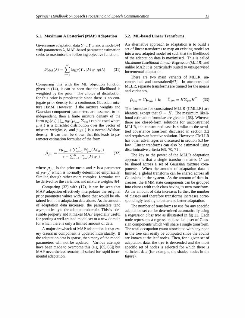
Given some adaptation dataY 1..Y R and a modelMwith parametersλ, MAP-based parameter estimationseeks to maximise the following objective function,

FMAP(λ) =R∑

r=1

log p(Y r|MWr)p(λ) (31)

Comparing this with the ML objection functiongiven in (14), it can be seen that the likelihood isweighted by the prior. The choice of distributionfor this prior is problematic since there is no con-jugate prior density for a continuous Gaussian mix-ture HMM. However, if the mixture weights andGaussian component parameters are assumed to beindependent, then a finite mixture density of theform pD(cj)

∏

m pW (µjm, Σjm) can be used wherepD(.) is a Dirichlet distribution over the vector ofmixture weightscj andpW (.) is a normal-Wishartdensity. It can then be shown that this leads to pa-rameter estimation formulae of the form

µjm =τµjm +

∑R

r=1 Θrjm(MWr

)

τ +∑R

r=1 Γrjm(MWr

)(32)

whereµjm is the prior mean andτ is a parameterof pW (.) which is normally determined empirically.Similar, though rather more complex, formulae canbe derived for the variances and mixture weights [64]

Comparing (32) with (17), it can be seen thatMAP adapation effectively interpolates the originalprior parameter values with those that would be ob-tained from the adaptation data alone. As the amountof adaptation data increases, the parameters tendasymptotically to the adaptation domain. This is a de-sirable property and it makes MAP especially usefulfor porting a well-trained model set to a new domainfor which there is only a limited amount of data.

A major drawback of MAP adaptation is that ev-ery Gaussian component is updated individually. Ifthe adaptation data is sparse, then many of the modelparameters will not be updated. Various attemptshave been made to overcome this (e.g. [65, 66]) butMAP nevertheless remains ill-suited for rapid incre-mental adaptation.

5.2. ML-based Linear Transforms

An alternative approach to adaptation is to build aset of linear transforms to map an existing model setinto a new adapted model set such that the likelihoodof the adaptation data is maximised. This is calledMaximum Likelihood Linear Regression(MLLR)andunlike MAP, it is particularly suited to unsupervisedincremental adaptation.

There are two main variants of MLLR: un-constrained and constrained[67]. In unconstrainedMLLR, separate transforms are trained for the meansand variances,

µjm = Gµjm + b; Σjm = HΣjmHT (33)

The formulae for constrained MLLR (CMLLR) areidentical except thatG = H . The maximum likeli-hood estimation formulae are given in [68]. Whereasthere are closed-form solutions for unconstrainedMLLR, the constrained case is similar to the semi-tied covariance transform discussed in section 3.2and requires an iterative solution. However, CMLLRhas other advantages as discussed in section 5.3 be-low. Linear tranforms can also be estimated usingdiscriminative criteria [69, 70, 71].

The key to the power of the MLLR adaptationapproach is that a single transform matrixG canbe shared across a set of Gaussian mixture com-ponents. When the amount of adaptation data islimited, a global transform can be shared across allGaussians in the system. As the amount of data in-creases, the HMM state components can be groupedinto classes with each class having its own transform.As the amount of data increases further, the numberof classes and therefore transforms increases corre-spondingly leading to better and better adaptation.

The number of transforms to use for any specificadaptation set can be determined automatically usinga regression class treeas illustrated in fig 11. Eachnode represents a regression class i.e. a set of Gaus-sian components which will share a single transform.The total occupation count associated with any nodein the tree can easily be computed since the countsare known at the leaf nodes. Then, for a given set ofadaptation data, the tree is descended and the mostspecific set of nodes is selected for which there issufficient data (for example, the shaded nodes in thefigure).


When used in unsupervised mode, MLLR isnormally applied iteratively[72]. First, the un-known test speech is recognised, then the hypothe-sised transcription is used to estimate MLLR trans-forms. The test speech is then re-recognised using theadapted models. This is repeated until convergence isachieved. A refinement of this is to use recognitionlattices in place of the 1-best hypothesis to accumu-late the adaptation statistics. This approach is morerobust to recognition errors and avoids the need tore-recognise the data since the lattice can simply berescored[73].

5.3. Adaptive Training

Ideally, an acoustic model set should encode justthose dimensions which allow the different classes tobe discriminated. However, in the case of speaker in-dependent (SI) speech recognition, the training datanecessarily includes a large number of speakers andhence acoustic models trained directly on this set willhave to “waste” a large number of parameters encod-ing the variablity between speakers rather than thevariability between spoken words which is the trueaim.

One way to overcome this is to replace the singleSI model set with a cluster of more specific modelswhere each model can be trained on more homoge-nous data. This is calledCluster Adaptive Train-ing (CAT). At recognition time, a linear combinationof models is selected where the set of interpolationweights, in effect, forms a speaker specific transform[74, 75, 76]. More recently discriminative techniqueshave been applied to CAT with some success [77].

An alternative approach to CAT is to use adap-tation to transform each training set speaker to forma canonical model. This is calledSpeaker AdaptiveTraining (SAT)and the conceptual schema for this isshown in Fig. 12 [78]. When only mean transforma-tions are used, SAT is straightforward. A transformis estimated for each speaker, and then the parame-ters of the canonical model set are estimated by mod-ifying the statistics to account for the tranform. Forexample, to estimate the canonical model means, thecounts in (15) and (16) are modified as follows:

Θrjm(M) =

Tr∑

t=1

γrjm(t)G(r) T Σ−1

jm(yrt − b(r))

∣

∣

∣

∣

∣

M

(34)and

Γrjm(M) =

Tr∑

t=1

γrjm(t)G(r) T Σ−1

jmG(r)

∣

∣

∣

∣

∣

M

(35)

whereG(r), b(r) is the transform for the speaker ut-tering training sentencer. The mean is then esti-mated using (17) as normal.

Rather than modifying the statistics, the use ofCMLLR allows adaptive training to be simplified fur-ther and allows combined mean and variance adap-tation. Similar to the case for semi-tied covariances,the CMLLR transformed likelihood can be computedsimply by regarding it as a feature space transforma-tion, i.e. for any mixture componetm of statej

N (y; µjm, Σjm) =1

|G|N (G−1(y − b); µjm, Σjm)

(36)whereµjm andΣjm are the transformed means andvariances as in (33) (withG = H)). Thus a SAT sys-tem can be built using CMMLR simply by iteratingbetween the estimation of the canonical model usingestimation of the transformed training data and thetransforms using the canonical model.

Finally, note that SAT trained systems incur theproblem that they can only be used once transformshave been estimated for the test data. Thus, an SImodel set is typically retained to generate the initialhypothesised transcription or lattice needed to com-pute the first set of transforms.

6. MULTI-PASS RECOGNITIONARCHITECTURES

The previous sections have reviewed some of the ba-sic techniques available for both training and adapt-ing a HMM-based recognition system. In general,any particular combination of model set and adap-tation technique will have slightly different charac-teristics and make different errors. Furthermore, ifthe outputs of these systems are converted to confu-sion networks as explained in section 2.4, then it is


straightforward to combine the confusion networksand then select the word sequence with the overallmaximum posterior likelihood. Thus, modern tran-scription systems typically utilise multiple model setsand make multiple passes over the data.

A typical architecture is shown in Fig. 13. A firstpass is made over the data using a relatively simple SImodel set. The 1-best output from this pass is usedto perform a first round of adaptation. The adaptedmodels are then used to generate lattices using a basicbigram or trigram word-based language model. Oncethe lattices have been generated, a range of morecomplex models and adaptation techniques can beapplied in parallel to providen candidate output con-fusion networks from which the best word sequenceis extracted. These 3rd pass models may include MLand MPE trained systems, SI and SAT trained mod-els, triphone and quinphone models, lattice-basedMLLR, CMLLR, 4-gram language models interpo-lated with class-ngrams and many other variants. Forexamples of recent large-scale transcription systemssee [11, 60, 79].

The gains obtained from this type of system com-bination can vary but overall performance is more ro-bust across a range of task domains. Finally, note thatadaptation can work more effectively if the requiredhypothesised transcriptions are generated by a differ-ent system. Thus, cross adaptation is also an increas-ingly popular architectural option.

7. CONCLUSIONS

This chapter has reviewed the core architecture ofa HMM-based CSR system and outlined the ma-jor areas of refinement incorporated into modern-day systems. Diagonal covariance continuous den-sity HMMs are based on the premise that each in-put frame is independent, its components are decor-related and have Gaussian distributions. Since noneof these assumptions are true, the various refine-ments described above can all be viewed as attemptsto reduce the impact of these false assumptions.Whilst many of the techniques are quite complex,they are nevertheless effective and overall substantialprogress has been made. For example, error rates onthe transcription of conversational telephone speechwere around 45% in 1995. Today, with the benefit ofmore data, and the refinements described above, error

rates are now well below 20%. Similarly, broadcastnews transcription has improved from around 30%WER in 1997 to below 15% today.

Despite their dominance and the continued rateof improvement, many argue that the HMM architec-ture is fundamentally flawed and performance mustasymptote. Of course, this is undeniably true sincewe have in our own heads an existence proof. How-ever, no good alternative to the HMM has been foundyet. In the meantime, the performance asymptoteseems to be still some way away.

8. REFERENCES

[1] JK Baker. The Dragon System - an Overview.IEEE Trans Acoustics Speech and Signal Pro-cessing, 23(1):24–29, 1975.

[2] F Jelinek. Continuous Speech Recognition byStatistical Methods. Proc IEEE, 64(4):532–556, 1976.

[3] BT Lowerre. The Harpy Speech RecognitionSystem. PhD thesis, Carnegie Mellon, 1976.

[4] LR Rabiner, B-H Juang, SE Levinson, andMM Sondhi. Recognition of Isolated Digits Us-ing HMMs with Continuous Mixture Densities.ATT Technical J, 64(6):1211–1233, 1985.

[5] LR Rabiner. A Tutorial on Hidden MarkovModels and Selected Applications in SpeechRecognition.Proc IEEE, 77(2):257–286, 1989.

[6] PJ Price, W Fisher, J Bernstein, and DS Pallet.The DARPA 1000-word Resource Managementdatabase for continuous speech recognition. InProc ICASSP, volume 1, pages 651–654, NewYork, 1988.

[7] SJ Young and LL Chase. Speech Recogni-tion Evaluation: A Review of the US CSR andLVCSR Programmes.Computer Speech andLanguage, 12(4):263–279, 1998.

[8] DS Pallet, JG Fiscus, J Garofolo, A Martin, andM Przybocki. 1998 Broadcast News Bench-mark Test Results: English and Non-EnglishWord Error Rate Performance Measures. Tech-nical report, National Institute of Standards andTechnology (NIST), 1998.

[9] JJ Godfrey, EC Holliman, and J McDaniel.SWITCHBOARD. InProc ICASSP, volume 1,pages 517–520, San Francisco, 1992.


[10] G Evermann, HY Chan, MJF Gales, T Hain,X Liu, D Mrva, L Wang, and P Woodland.Development of the 2003 CU-HTK Conversa-tional Telephone Speech Transcription System.In Proc. ICASSP, Montreal, Canada, 2004.

[11] H Soltau, B Kingsbury, L Mangu, D Povey,G Saon, and G Zweig. The IBM 2004 Conver-sational Telephony System for Rich Transcrip-tion. In Proc ICASSP, Philadelphia, PA, 2005.

[12] SJ Young et al. The HTK BookVersion 3.4. Cambridge University,http://htk.eng.cam.ac.uk, 2006.

[13] SJ Young. Large Vocabulary ContinuousSpeech Recognition.IEEE Signal ProcessingMagazine, 13(5):45–57, 1996.

[14] SB Davis and P Mermelstein. Comparisonof Parametric Representations for Monosyl-labic Word Recognition in Continuously Spo-ken Sentences.IEEE Trans Acoustics Speechand Signal Processing, 28(4):357–366, 1980.

[15] H Hermansky. Perceptual Linear Predictive(PLP) Analysis of Speech.J Acoustical Soci-ety of America, 87(4):1738–1752, 1990.

[16] AP Dempster, NM Laird, and DB Rubin. Max-imum likelihood from incomplete data via theEM algorithm. J Royal Statistical Society Se-ries B, 39:1–38, 1977.

[17] SJ Young, JJ Odell, and PC Woodland. Tree-Based State Tying for High Accuracy AcousticModelling. InProc Human Language Technol-ogy Workshop, pages 307–312, Plainsboro NJ,Morgan Kaufman Publishers Inc, 1994.

[18] X Luo and F Jelinek. Probabilistic Classifi-cation of HMM States for Large Vocabulary.In Proc Int Conf Acoustics, Speech and SignalProcessing, pages 2044–2047, Phoenix, USA,1999.

[19] SM Katz. Estimation of Probabilities fromSparse Data for the Language Model Compo-nent of a Speech Recogniser.IEEE Trans ASSP,35(3):400–401, 1987.

[20] H Ney, U Essen, and R Kneser. On StructuringProbabilistic Dependences in Stochastic Lan-guage Modelling.Computer Speech and Lan-guage, 8(1):1–38, 1994.

[21] SF Chen and J Goodman. An EmpiricalStudy of Smoothing Techniques for Language

Modelling. Computer Speech and Language,13:359–394, 1999.

[22] PF Brown, VJ Della Pietra, PV de Souza,JC Lai, and RL Mercer. Class-based n-gramModels of Natural Language.ComputationalLinguistics, 18(4):467–479, 1992.

[23] R Kneser and H Ney. Improved Cluster-ing Techniques for Class-based Statistical Lan-guage Modelling. InProc Eurospeech, pages973–976, Berlin, 1993.

[24] S Martin, J Liermann, and H Ney. Algorithmsfor Bigram and Trigram Word Clustering. InProc Eurospeech’95, volume 2, pages 1253–1256, Madrid, 1995.

[25] SJ Young, NH Russell, and JHS Thorn-ton. Token Passing: a Simple Concep-tual Model for Connected Speech Recogni-tion Systems. Technical Report CUED/F-INFENG/TR38, Cambridge University Engi-neering Department, 1989.

[26] K Demuynck, J Duchateau, and D van Com-pernolle. A Static Lexicon Network Repre-sentation for Cross-Word Context DependentPhones. InProc Eurospeech, pages 143–146,Rhodes, Greece, 1997.

[27] SJ Young. Generating Multiple Solutions fromConnected Word DP Recognition Algorithms.In Proc IOA Autumn Conf, volume 6, pages351–354, 1984.

[28] H Thompson. Best-first enumeration of pathsthrough a lattice - an active chart parsingsolution. Computer Speech and Language,4(3):263–274, 1990.

[29] F Richardson, M Ostendorf, and JR Rohlicek.Lattice-Based Search Strategies for Large Vo-cabulary Recognition. InProc ICASSP, vol-ume 1, pages 576–579, Detroit, 1995.

[30] L Mangu, E Brill, and A Stolcke. Finding Con-sensus Among Words: Lattice-based Word Er-ror Minimisation. Computer Speech and Lan-guage, 14(4):373–400, 2000.

[31] G Evermann and PC Woodland. Posterior Prob-ability Decoding, Confidence Estimation andSystem Combination. InProc. Speech Tran-scription Workshop, Baltimore, 2000.

[32] G Evermann and PC Woodland. Large vo-cabulary decoding and confidence estimation


using word posterior probabilities. InProc.ICASSP 2000, pages 1655–1658, Istanbul,Turkey, 2000.

[33] V Goel, S Kumar, and B Byrne. SegmentalMinimum Bayes-Risk ASR Voting Strategies.In ICSLP, 2000.

[34] J Fiscus. A Post-Processing System to YieldReduced Word Error Rates: Recogniser Out-put Voting Error Reduction (ROVER). InProcIEEE ASRU Workshop, pages 347–352, SantaBarbara, 1997.

[35] D Hakkani-Tur, F Bechet, G Riccardi, andG Tur. Beyond ASR 1-best: Using word confu-sion networks in spoken language understand-ing . Computer Speech and Language, In press,2006.

[36] JJ Odell, V Valtchev, PC Woodland, andSJ Young. A One-Pass Decoder Design forLarge Vocabulary Recognition. InProc HumanLanguage Technology Workshop, pages 405–410, Plainsboro NJ, Morgan Kaufman Publish-ers Inc, 1994.

[37] X Aubert and H Ney. Large Vocabulary Contin-uous Speech Recognition Using Word Graphs.In Proc ICASSP, volume 1, pages 49–52, De-troit, 1995.

[38] M Mohri, F Pereira, and M Riley. WeightedFinite State Transducers in Speech Recognition.Computer Speech and Language, 16(1):69–88,2002.

[39] F Jelinek. A Fast Sequential Decoding Algo-rithm Using a Stack.IBM J Research and De-velopment, 13, 1969.

[40] DB Paul. Algorithms for an Optimal A*Search and Linearizing the Search in the StackDecoder. InProc ICASSP, pages 693–996,Toronto, 1991.

[41] A Nadas. A Decision Theoretic Formula-tion of a Training Problem in Speech Recogni-tion and a Comparison of Training by Uncon-ditional Versus Conditional Maximum Likeli-hood.IEEE Trans Acoustics Speech and SignalProcessing, 31(4):814–817, 1983.

[42] B-H Juang, SE Levinson, and MM Sondhi.Maximum Likelihood Estimation for Multivari-ate Mixture Observations of Markov Chains.IEEE Trans Information Theory, 32(2):307–

309, 1986.[43] LR Bahl, PF Brown, PV de Souza, and RL Mer-

cer. Maximum Mutual Information Estima-tion of Hidden Markov Model Parameters forSpeech Recognition. InProc ICASSP, pages49–52, Tokyo, 1986.

[44] V Valtchev, JJ Odell, PC Woodland, andSJ Young. MMIE Training of Large VocabularyRecognition Systems.Speech Communication,22:303–314, 1997.

[45] R Schluter, B Muller, F Wessel, and H Ney.Interdependence of Language Models and Dis-criminative Training. InProc IEEE ASRUWorkshop, pages 119–122, Keystone, Col-orado, 1999.

[46] P Woodland and D Povey. Large Scale Dis-criminative Training of Hidden Markov Modelsfor Speech Recognition.Computer Speech andLanguage, 16:25–47, 2002.

[47] W Chou, C H Lee, and BH Juang. MinimumError Rate Training Based on N-best StringModels. InProc ICASSP 93, pages p652–655,Minneapolis, 1993.

[48] D Povey and P Woodland. Minimum PhoneError and I-Smoothing for Improved Discrim-inative Training. InProc ICASSP, Orlando,Florida, 2002.

[49] PS Gopalakrishnan, D Kanevsky, A Nadas,D Nahamoo, and MA Picheny. Decoder Selec-tion based on Cross-Entropies. InProc ICASSP,volume 1, pages 20–23, New York, 1988.

[50] PC Woodland and D Povey. Large ScaleDiscriminative Training for Speech Recogni-tion. In ISCA ITRW Automatic Speech Recogni-tion: Challenges for the Millenium, pages 7–16,Paris, 2000.

[51] MJF Gales. Semi-tied Covariance Matrices ForHidden Markov Models. IEEE Trans Speechand Audio Processing, 7(3):272–281, 1999.

[52] AV Rosti and M Gales. Factor Analysed Hid-den Markov Models for Speech Recognition.Computer Speech and Language, 18(2):181–200, 2004.

[53] S Axelrod, R Gopinath, and P Olsen. Modelingwith a Subspace Constraint on Inverse Covari-ance Matrices. InICSLP 2002, Denver, CO,2002.


[54] P Olsen and R Gopinath. Modeling Inverse Co-variance Matrices by Basis Expansion. InProcICSLP 2002, Denver, CO, 2002.

[55] N Kumar and AG Andreou. Heteroscedasticdiscriminant analysis and reduced rank HMMsfor improved speech recognition.Speech Com-munication, 26:283–297, 1998.

[56] MJF Gales. Maximum Likelihood MultipleSubspace Projections for Hidden Markov Mod-els. IEEE Trans Speech and Audio Processing,10(2):37–47, 2002.

[57] T Hain, PC Woodland, TR Niesler, and EWDWhittaker. The 1998 HTK System for Tran-scription of Conversational Telephone Speech.In Proc IEEE Int Conf Acoustics Speechand Signal Processing, pages 57–60, Phoenix,1999.

[58] G Saon, A Dharanipragada, and D Povey. Fea-ture Space Gaussianization. InProc ICASSP,Montreal, Canada, 2004.

[59] SS Chen and R Gopinath. Gaussianization. InNIPS 2000, Denver, Colorado, 2000.

[60] MJF Gales, B Jia, X Liu, KC Sim, P Wood-land, and K Yu. Development of the CUHTK2004 RT04 Mandarin Conversational Tele-phone Speech Transcription System. InProc.ICASSP, Philadelphia, PA, 2005.

[61] L Lee and RC Rose. Speaker Normalisation Us-ing Efficient Frequency Warping Procedures. InICASSP’96, Atlanta, 1996.

[62] J McDonough, W Byrne, and X Luo. SpeakerNormalisation with All Pass Transforms. InProc ISCLP98, Sydney, 1998.

[63] DY Kim, S Umesh, MJF Gales, T Hain, andP Woodland. Using VTLN for Broadcast NewsTranscription. InICSLP04, Jeju, Korea, 2004.

[64] J-L Gauvain and C-H Lee. Maximum a Poste-riori Estimation of Multivariate Gaussian Mix-ture Observations of Markov Chains.IEEETrans Speech and Audio Processing, 2(2):291–298, 1994.

[65] SM Ahadi and PC Woodland. CombinedBayesian and Predictive Techniques for RapidSpeaker Adaptation of Continuous DensityHidden Markov Models.Computer Speech andLanguage, 11(3):187–206, 1997.

[66] K Shinoda and C H Lee. Structural MAPSpeaker Adaptation using Hierarchical Priors.In Proc ASRU’97, Santa Barbara, 1997.

[67] CJ Leggetter and PC Woodland. Maxi-mum Likelihood Linear Regression for SpeakerAdaptation of Continuous Density HiddenMarkov Models. Computer Speech and Lan-guage, 9(2):171–185, 1995.

[68] MJF Gales. Maximum Likelihood Lin-ear Transformations for HMM-Based SpeechRecognition.Computer Speech and Language,12:75–98, 1998.

[69] F Wallhof, D Willett, and G Rigoll. Frame-discriminative and Confidence-driven Adapta-tion for LVCSR. In Proc ICASSP’00, pages1835–1838, Istanbul, 2000.

[70] L Wang and P Woodland. Discriminative Adap-tive Training using the MPE Criterion. InProcASRU, St Thomas, US Virgin Islands, 2003.

[71] S Tsakalidis, V Doumpiotis, and WJ Byrne.Discriminative Linear Transforms for Fea-ture Normalisation and Speaker Adaptation inHMM Estimation. IEEE Trans Speech and Au-dio Processing, 13(3):367–376, 2005.

[72] P Woodland, D Pye, and MJF Gales. Itera-tive Unsupervised Adaptation using MaximumLikelihood Linear Regression. InICSLP’96,pages 1133–1136, Philadelphia, 1996.

[73] M Padmanabhan, G Saon, and G Zweig.Lattice-based Unsupervised MLLR for SpeakerAdaptation. InProc ITRW ASR2000: ASRChallenges for the New Millenium, pages 128–132, Paris, 2000.

[74] TJ Hazen and J Glass. A Comparison of NovelTechniques for Instantaneous Speaker Adapta-tion. InProc Eurospeech’97, pages 2047–2050,1997.

[75] R Kuhn, L Nguyen, J-C Junqua, L Goldwasser,N Niedzielski, S Finke, K Field, and M Con-tolini. Eigenvoices for Speaker Adaptation. InICSLP’98, Sydney, 1998.

[76] MJF Gales. Cluster Adaptive Training of Hid-den Markov Models.IEEE Trans Speech andAudio Processing, 8:417–428, 2000.

[77] K Yu and MJF Gales. Discriminative ClusterAdaptive Training.IEEE Trans Speech and Au-dio Processing, 2006.


[78] T Anastasakos, J McDonough, R Schwartz, andJ Makhoul. A Compact Model for SpeakerAdaptive Training. InICSLP’96, Philadelphia,1996.

[79] R Sinha, MJF Gales, DY Kim, X Liu, KC Sim,and PC Woodland. The CU-HTK MandarinBroadcast News Transcription System. InICASSP’06, Toulouse, 2006.


Feature Extraction

Decoder Y W

Speech Feature Vectors Words

"Stop that."

Acoustic Models

Pronunciation Dictionary

Language Model

Figure 1: Architecture of a HMM-based Recogniser

a aa22

a12 a23 a34 a45

33 44

1 2 3 4 5

Y

2

y1 y2 y3 y4 y5

1b2y( ) b2y( ) 3( )b3y ( )b4y4 ( )b4y5

=

AcousticVector

Sequence

Markov Model

Figure 2: HMM-based Phone Model

(silence) Stop that (silence)

sil s t oh p th ae t sil

m1 m23 m94 m32 m34 m984 m763 m2 m1

W

Q

L

P

sil sil -s+ t s- t +oh t -oh+p oh-p+ th p- th + ae th - ae + t ae - t + sil sil

Figure 3: Context Dependent Phone Modelling


t-ih+n t-ih+ng f-ih+l s-ih+l

t-ih+n t-ih+ng f-ih+l s-ih+l

Tie similar states

Figure 4: Formation of Tied-State Phone Models

s- aw + n

t - aw + n

s- aw + t

etc 1 2 3

5 4 3 2 1

n y

R=central-cons?

y

y

n n

n

L =nasal? R=nasal?

L =central-stop?

states in each leaf node are tied

base phone = aw

Figure 5: Decision Tree Clustering


ax

ax

ax

z eh n

b oa t

b

....

ax

a

abort

zen Start

Token End

Token

ow t about

Figure 6: Basic Recognition Network

Put a start token < log(1), ∅ > in network entry node;Put null tokens < log(0), ∅ > in all other nodes;for each time t = 1 to T do

– word internal token propagationfor each non-entry node j do

MaxP = log(0);for each predecessor node i do

Temp token Q = Qi;Q.LogP += log(aij) [+ log(bj(yt)) if j emitting ];If Q.LogP > MaxP then

Qj = Q; MaxP = Q.LogP ;end;

end;Copy tokens from word internal exits to following entries;– word external token propagationfor each word w with entry node j do

MaxP = log(0);for each predecessor word u with exit node i do

Temp token Q = Qi;Q.LogP += α log p(w|u) + β;If Q.LogP > MaxP then

Qj = Q; MaxP = Q.LogP ; u′ = u

end;– Record word boundary decisionCreate a record R;R.Q = Qj ; R.t = t; R.word = u′;Q.link =↑ R;

end;Put null token in network entry node;

end;Token in network exit state at time T represents the best path;

Figure 7: Basic Token Passing Algorithm


ax

z eh n

b oa t

....

a

abort

zen Start

Token End

Token

ow t about

Figure 8: Tree-Structured Recognition Network

HAVE

HAVE HAVE

I

I MOVE

VERY

VERY

I SIL

SIL

VEAL

OFTEN

OFT

EN

SIL

SIL SIL

SIL

FINE

IT VERY FINE

FAST

VER

Y

MOVE

HAVE IT

(a) Word Lattice

I HAVE IT VEAL FINE

- MOVE - VERY OFTEN

FAST

(b) Confusion Network

Time

Figure 9: Example Lattice and Confusion Network


Warped Frequency

Actual Frequency

(b)

f low f high

Warped Frequency

Actual Frequency

male

female

warp factor

(a) male

female

Figure 10: Vocal Tract Length Normalisation

...

Global Class

Base classes - one per Gaussian

... ...

Figure 11: A Regression Class Tree

Speaker 1 Transform

Speaker N Transform

Canonical Model

Speaker 1 Model

Speaker 2 Transform

Speaker 2 Model

Speaker N Model

...

Data for Speaker 1

Data for Speaker 2

Data for Speaker N

... ...

Figure 12: Adaptive Training


Pass 1: Initial Transcription

Pass 2: Lattice Generation

Adapt

P3.1

Adapt

P3.n

...

Lattices

Combine

Figure 13: Multi-pass/System Combination Architecture

Indexadaptation, 15

backing-off, 5base phones, 3Baum-Welch, 8Bayes’ Rule, 2beam search, 6bigram, 7, 9

cepstral mean normalisation, 11class-based language model, 5cluster adaptive training (CAT), 14confusion network, 7conjugate prior, 13constrained MLLR, 13, 14covariance modelling, 10

dictionary, 2discriminative training, 8dynamic network decoder, 8dynamic programming, 5

extended Baum-Welch, 9

feature extraction, 2forward-backward algorithm, 3, 8

Gaussianization, 11

H-criterion, 10heteroscedastic LDA (HLDA), 11hidden Markov model toolkit (HTK), 1, 11

I-smoothing, 10

Jacobean, 12

language model, 2, 5language model look-ahead, 6language model scaling, 2lattice-baed MMI, 9linear prediction, 2linear transform, 10logical model, 4

MAP adaptation, 13maximum likelihood, 8

maximum likelihood linear regression (MLLR), 13maximum mutual information (MMI), 8mel-frequency cepstral coefficients (MFCCs), 2minimum classification error (MCE), 9minimum phone error, 9mixture of Gaussians, 3mixture splitting, 4monophones, 3

N-gram, 5N-gram smoothing, 5

perceptual linear prediction (PLP), 2phone, 2phonetic decision tree, 4phonological processes, 4physical model, 4pronunciation dictionary, 4pronunciation variation, 3, 9

raw phone accuracy, 9regression coefficients, 2regression tree, 13

semi-tied covariance, 10speaker adaptive training, 14stack decoder, 8state clustering, 4structured covariance, 10system combination, 15

tied-state triphones, 4token, 6token-passing, 6triphones, 3

variance normalisation, 11Viterbi algorithm, 6vocal tract length normalisation (VTLN), 12

Wishart density, 13word insertion penalty, 2word lattice, 7, 9word-link record, 6

26

hmms and related speech recognition technologies - CiteSeerX

Documents

Transcript of hmms and related speech recognition technologies - CiteSeerX