Input�Output HMMs for Sequence Processing

Yoshua Bengio� Paolo Frasconi

Dept� Informatique et Dipartimento di Sistemi

Recherche Op�erationnelle e Informatica

Universit�e de Montr�eal Universit�a di Firenze

Montreal� Qc H�C��J� ��� Firenze �Italy�

September � �

Abstract

We consider problems of sequence processing and propose a solution based on a discrete state model

in order to represent past context� We introduce a recurrent connectionist architecture having a modular

structure that associates a subnetwork to each state� The model has a statistical interpretation we call

Input�Output Hidden Markov Model �IOHMM�� It can be trained by the EM or GEM algorithms�

considering state trajectories as missing data� which decouples temporal credit assignment and actual

parameter estimation�

The model presents similarities to hidden Markov models �HMMs�� but allows us to map input se�

quences to output sequences� using the same processing style as recurrent neural networks� IOHMMs are

trained using a more discriminant learning paradigm than HMMs� while potentially taking advantage

of the EM algorithm�

We demonstrate that IOHMMs are well suited for solving grammatical inference problems on a

benchmark problem� Experimental results are presented for the seven Tomita grammars� showing that

these adaptive models can attain excellent generalization�

�also� AT�T Bell Laboratories� Holmdel� NJ

�

� Introduction

For many learning problems� the data of interest have a signi�cant sequential structure� Problems of

this kind arise in a variety of applications� ranging from written or spoken language processing� to the

production of actuator signals in control tasks� to multivariate time�series prediction� Feedforward neural

networks are inadequate in many of these cases because of the absence of a memory mechanism that can

retain past information in a �exible way� Even if these models include delays in their connections ���� the

duration of the temporal contingencies that can be captured is �xed a priori by the architecture rather

than being inferred from data� Furthermore� for some tasks� the appropriate size of the input window

�or delays varies during the sequence or from sequence to sequence� Recurrent neural networks� on the

other hand� allow one to model arbitrary dynamical systems �� �� and can store and retrieve contextual

information in a very �exible way� i�e�� for durations that are not �xed a priori and that can vary from one

sequence to another� In sequence analysis systems that can take context into account in a �exible manner

�such as recurrent neural networks and HMMs� one �nds some form of �state variable or representation

of past context� With a state�space representation the main computations can be divided into �� updating

the state or context variable �the state transition function� and � computing or predicting an output�

given the current state �the output function�

Up to now� research e�orts on supervised learning for recurrent networks have been almost exclusively

focused on gradient descent methods and a continuous state�space� Numerous algorithms are available

for computing the gradient� For example� the back�propagation through time �BPTT algorithm ��� �� is

a straightforward generalization of back�propagation that allows one to compute the complete gradient

in fully recurrent networks� The real time recurrent learning �RTRL algorithm ��� �� �� is local in time

and produces a partial gradient after each time step� thus allowing on�line weights updating� Another

algorithm was proposed for training local feedback recurrent networks ��� ���� It is also local in time�

but requires computation only proportional to the number of weights� like back�propagation through

time� Local feedback recurrent networks are suitable for implementing short�term memories but they

have limited representational power for dealing with general sequences ���� ���

However� practical di�culties have been reported in training recurrent neural networks to perform tasks

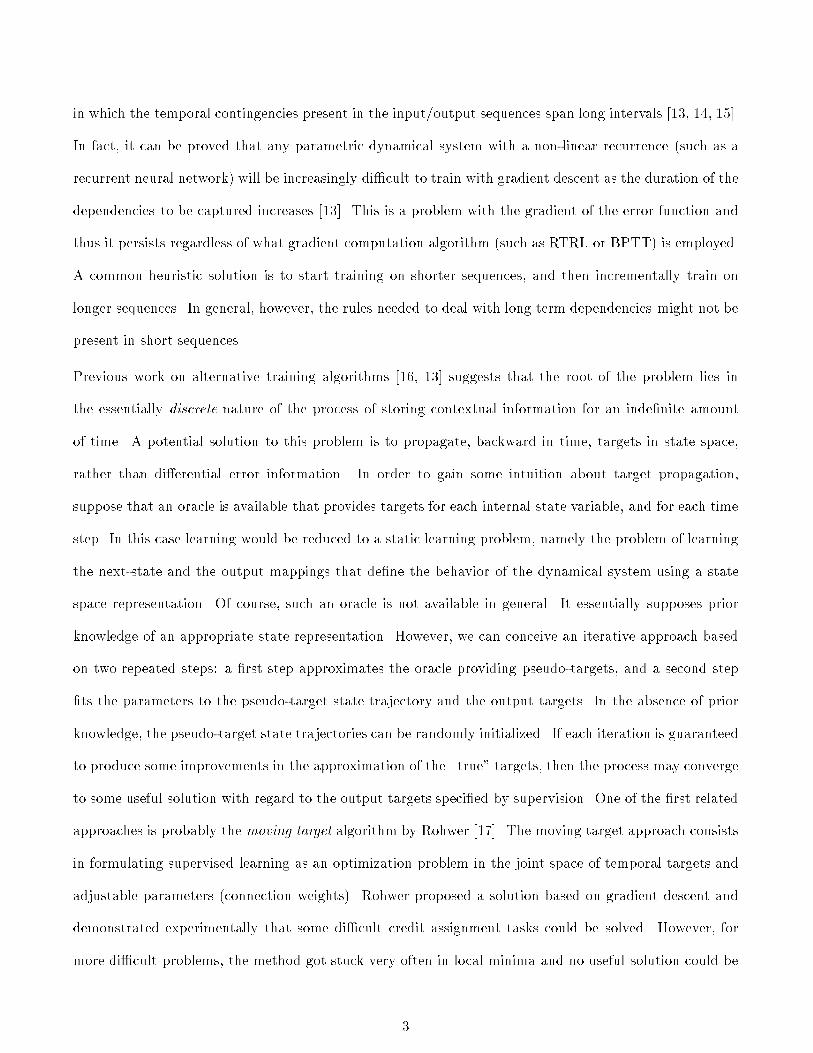
in which the temporal contingencies present in the input�output sequences span long intervals ���� ��� ����

In fact� it can be proved that any parametric dynamical system with a non�linear recurrence �such as a

recurrent neural network will be increasingly di�cult to train with gradient descent as the duration of the

dependencies to be captured increases ����� This is a problem with the gradient of the error function and

thus it persists regardless of what gradient computation algorithm �such as RTRL or BPTT is employed�

A common heuristic solution is to start training on shorter sequences� and then incrementally train on

longer sequences� In general� however� the rules needed to deal with long term dependencies might not be

present in short sequences�

Previous work on alternative training algorithms ���� ��� suggests that the root of the problem lies in

the essentially discrete nature of the process of storing contextual information for an inde�nite amount

of time� A potential solution to this problem is to propagate� backward in time� targets in state space�

rather than di�erential error information� In order to gain some intuition about target propagation�

suppose that an oracle is available that provides targets for each internal state variable� and for each time

step� In this case learning would be reduced to a static learning problem� namely the problem of learning

the next�state and the output mappings that de�ne the behavior of the dynamical system using a state

space representation� Of course� such an oracle is not available in general� It essentially supposes prior

knowledge of an appropriate state representation� However� we can conceive an iterative approach based

on two repeated steps� a �rst step approximates the oracle providing pseudo�targets� and a second step

�ts the parameters to the pseudo�target state trajectory and the output targets� In the absence of prior

knowledge� the pseudo�target state trajectories can be randomly initialized� If each iteration is guaranteed

to produce some improvements in the approximation of the �true targets� then the process may converge

to some useful solution with regard to the output targets speci�ed by supervision� One of the �rst related

approaches is probably the moving target algorithm by Rohwer ����� The moving target approach consists

in formulating supervised learning as an optimization problem in the joint space of temporal targets and

adjustable parameters �connection weights� Rohwer proposed a solution based on gradient descent and

demonstrated experimentally that some di�cult credit assignment tasks could be solved� However� for

more di�cult problems� the method got stuck very often in local minima and no useful solution could be

�

obtained�

Extending previous work ����� in this paper we propose a statistical approach to target propagation�

based on the EM algorithm� We consider a parametric dynamical system having n discrete states and we

introduce a modular architecture� with subnetworks associated to discrete states� The architecture can be

interpreted as a statistical model and can be trained by the EM or generalized EM �GEM algorithms of

Dempster� Laird� � Rubin ����� by considering the internal state trajectories as missing data� In this way

learning is factored into a temporal credit assignment subproblem and a static learning subproblem that

consists in �tting parameters to the next�state and output mappings de�ned by the estimated trajectories�

In order to iteratively tune parameters with the EM or GEM algorithms� the system propagates forward

and backward a discrete distribution over the n states� resulting in a procedure similar to the Baum�Welsh

algorithm used to train standard hidden Markov models �HMMs ��� �� ��

The main di�erence between standard HMMs and the model presented here� is that the former represent

the distribution P �yT� of output sequences yT� � y��y�� � � � �yT � whereas the latter represents the condi�

tional distribution P �yT� j uT� of output sequences given input sequences u

T� � u��u�� � � � �uT � The model

presented here is therefore called Input�Output HMM� or IOHMM� IOHMMs are trained by maximizing

the conditional likelihood P �yT� j uT� � This is a supervised learning problem since the output sequence

yT� plays the role of a desired output in response to the input sequence uT� � If the output represents clas�

si�cation decisions to be made when the input sequence is given� this approach is more discriminant than

standard HMMs �trained to maximize the likelihood of the observations� For example� in applications

of HMMs to isolated word recognition �a special case of sequence classi�cation� a separate model is con�

structed for each word �class and trained on instances of that class only� This type of training is said to

be not discriminant because each model �in our example� each word model is trained independently� we

try to model the type of observations �here� acoustic representative of that class �here� word� Instead�

discriminant training strategies do not attempt to build the best model of observations for each class�

but rather focus on on the di�erences between the type of observations for each class� in order to better

predict whether a given observation belongs to one class or another� Thus� models trained by discriminant

approaches can be expressed with less degrees of freedom� since they concentrate the use of parameters

�

on the decision surface between the classes� rather than on the distribution of data everywhere� Another

advantage of more discriminant training criteria is that they tend to be more robust to incorrectness of

the model� and for this reason sometimes perform better ��� ���

Both the input and output sequences can be multivariate� discrete or continuous� Thus IOHMMs can

perform sequence regression �y continuous or classi�cation �y discrete� For example� in a task such as

phoneme recognition� uT� may be a sequence of acoustic vectors �such as cepstral parameters and y

T� may

consist of a discrete sequence of phonetic labels� In sequence classi�cation tasks �such as isolated word

recognition� the output can be the label yT of a class� de�ned only at the end of each sequence� Other

potential �elds of application are robot navigation� system identi�cation� and time�series prediction� For

example� for economic time�series� the input sequences could be di�erent economic time�series� the output

sequence could be a prediction for the future values of some of these variables� and the hidden states could

represent di�erent regimes of the economy �e�g�� business cycles� For applications such as handwriting or

speech recognition� the output sequence �e�g�� a sequence of characters or phonemes does not have to be

synchronized with the input sequence �e�g�� pen trajectory or acoustic sequence�

Like in HMMs� using Markov assumptions� the distribution of outputs given the inputs can be factored

into sums of products of two types of factors� output probabilities and transition probabilities�

�� P �yt j xt�ut is the output distribution given the state xt and input ut at time t� This speci�es the

output function of the dynamical system�

� P �xt j xt���ut is the matrix of transition probabilities at time t� conditioned on current input ut�

This speci�es the state transition function of the dynamical system�

Therefore� a simple way to obtain an IOHMM from an HMM is to make the output and transition

probabilities function of an input ut at each time step t� The output distribution P �yt jut is obtained as

a mixture of probabilities ���� in which each component is conditional on a particular discrete state� and

the mixing proportions are the current state probabilities� conditional on the input� Hence� the model

has also interesting connections to the mixture of experts �ME architecture by Jacobs� Jordan� Nowlan

� Hinton ���� Like in the mixture of experts� sequence regression is carried out by associating di�erent

�

modules to di�erent states and letting each module �t the data �e�g�� compute the expected value of the

output given the state and input� E�yt j xt�ut� during the interval of time when it receives credit� As

in the mixture of experts� the task decomposition is smooth� Unlike the related approach of ���� the

gating �or switching between experts is provided by expert modules �one per state i computing the state

transition distribution P �xt j xt���i�ut �conditioned on the current input�

Another connectionist model extending hidden Markov models to process discrete input and output

streams was proposed in ���� for modeling the distribution of an output sequence y given an input

sequence u�

Other interesting related models are the various hybrids of neural networks and HMMs that have been

proposed in the literature �such as ��� ��� ��� ��� As in IOHMMs with neural networks for modeling

the transition and output distributions� for all of these models� the strictly neural part of the model is

feedforward �or has a short horizon� whereas the HMM is used to represent the longer�term temporal

structure �and in the case of speech� the prior knowledge about this structure�

Experiments on arti�cial tasks ���� have shown that a simpli�ed version of the approach presented here can

deal with long�term dependencies more e�ectively than recurrent networks trained with back�propagation

through time or other alternative algorithms� The model used in ���� has very limited representational

capabilities and can only map an input sequence to a �nal discrete state� In the present paper we describe

an extended architecture that allows one to fully specify both the input and output portions of data�

as required by the supervised learning paradigm� In this way� general sequence processing tasks can be

addressed� such as production� classi�cation� or prediction�

The paper is organized as follows� Section is devoted to a circuit description of the architecture and its

statistical interpretation� In section � we derive the equations for training IOHMMs� In particular� we

present an EM version of the learning algorithm that can be used for discrete inputs and linear subnetworks�

and a GEM version for general multilayered subnetworks� In section � we compare IOHMMs to other

related models for sequence processing� such as standard HMMs and other recurrent Mixture of Experts

architectures� In section � we analyze from a theoretical point of view the learning capabilities of the

model in the presence of long�term dependencies� arguing that improvements can be achieved by adding

�

an extra term to the likelihood function and�or by constraining the state transitions of the model� Finally�

in section � we report experimental results for a classical benchmark study in grammatical inference

�Tomita�s grammars� The results demonstrate that the model can achieve very good generalization using

few training examples�

� Input�Output Hidden Markov Models

��� The Proposed Architecture

Whereas recurrent networks usually have a continuous state space� in IOHMMs we will consider a proba�

bility distribution over a discrete state dynamical system� based on the following state space description�

xt � f�xt���ut

yt � g�xt�ut

��

where ut � Rm is the input vector at time t� yt � Rr is the output vector� and

xt � V � f�� � � � � � ng is a discrete state� These equations de�ne a generalized Mealy �nite state machine�

in which inputs and outputs may take on continuous values� f�� is referred to as the state transition func�

tion and g�� is the output function� In this paper� we consider a probabilistic version of these dynamics�

where the current inputs and the current state distribution are used to estimate the output distribution

and the state distribution for the next time step�

Admissible state transitions will be speci�ed by a transition graph G � fV � �Eg� whose vertices correspond

to the model�s states� G describes the topology of the underlying Markov model� A transition from state

j to state i is admissible if and only if there exists an edge eij � �E � We de�ne the set of successors for

each state j as� Sjdef� fi � V � �eij � �Eg�

The proposed system is illustrated in Figure �� The architecture is composed by a set of state networks

N j � j � � � � �n and a set of output networks Oj � j � � � � �n� Each one of the state and output networks is

uniquely associated to one of the states in V � and all networks share the same input ut� Each state network

Nj has the task of predicting the next state distribution P �xt j xt���i�ut� based on the current input and

given that the previous state xt�� � j� Similarly� each output network Oj computes some parameters of

�

)

, )

tt

...1 n

...O1

On

N N

current input t

t t

delay

)

current state distribution

current expected output, given past input sequence

softmax softmax

convexweighted sum

convexweighted sum

1t−1

t1,tϕ

ζ =tη =

t

1,tη =

t

t−1ζ =

t−1

t

=

P(x |

x = 1

P(x |

1u

t1

u

tu

tu

u

u

x =1t−1P( x | E[y | , ]

E[y | ]

Figure �� The proposed architecture� IOHMM and recurrent mixture of experts�

the distribution for the current output of the system� P �yt j xt�i�ut� given the current state and input�

Typically� the output networks compute the expected output value� �i�t � E�yt j xt � i�ut��

All the subnetworks are assumed to be static� i�e�� they are de�ned by means of algebraic mappings

Nj�ut� �j and Oj�ut��j� where �j and �j are vectors of adjustable parameters �e�g�� connection weights�

We assume that these functions are di�erentiable with respect to their parameters� The ranges of the

functions Nj� may be constrained in order to account for the underlying transition graph G� Each output

�ij�t of the state subnetwork Nj is associated to one of the successors i of state j� Thus the last layer

of Nj has as many units as the cardinality of Sj� For convenience of notation� we suppose that �ij�t are

de�ned for each i� j � �� � � � � n and we impose the condition �ij�t � � for each i not belonging to Sj� To

guarantee that the variables �ij�t are positive and summing to �� the softmax function ���� is used in the

last layer�

�ij�t �eaij�tX

��Sj

ea�j�t� j � �� � � � � n� i � Sj �

where aij�t are intermediate variables that can be thought of as the activations �e�g� weighted sums of the

�

output units of subnetwork N j � In this way�

nXi��

�ij�t � � �j� t� ��

and � can be given a probabilistic interpretation� As shown in Figure �� the outputs � of the state

networks are used to recursively compute at each time step the vector �t � Rn� which represents the

current �memory of the system� and can be interpreted as the current state distribution� given the past

input sequence� This �memory variable is computed as a linear combination of the outputs of the state

networks� gated by its value at the previous time step�

�t �nX

j��

�j�t�� �j�t ��

where �j�t � ���j�t� � � � � �nj�t���

Output networks compete to predict the global output of the system �t � Rr�

�t �nX

j��

�j�t�j�t ��

where �j�t � Rr is the output of subnetwork Oj �

At this level of description� we do not need to further specify the internal architecture of the state and

output subnetworks� as long as they compute a di�erentiable function of their parameters�

��� A Probabilistic Model

As hinted above� this connectionist architecture can be also interpreted as a probability model� To simplify�

we assume here a multinomial distribution for the state variable xt� i�e�� a probability is computed for each

possible value of the state variable xt� Let us consider �t� the main variable of the temporal recurrence

�t �Pn

j�� �j�t���j�t� If we initialize the vector �� to positive numbers summing to �� it can be interpreted

as a vector of initial state probabilities� Because �� is a convex sum� �t is a vector of positive numbers

summing to � for each t� and it will be given the following interpretation�

�i�t � P�xt � i j ut� ��

having denoted by ut� the subsequence of inputs from time � to t� inclusively� When making certain

conditional independence assumptions described in the next section� equation �� then has the following

�

probabilistic interpretation�

P �xt � i j ut� �

nXj��

P �xt � i j xt���j�utP �xt���j j ut��� ��

i�e�� the subnetworks N j compute transition probabilities conditioned on the input ut�

�ij�t � P�xt � i j xt�� � j�ut ��

As in neural networks trained to minimize the output mean squared error �MSE� the output �t of this

architecture can be interpreted as an expected �position parameter for the probability distribution of the

output yt� However� in addition to being conditional on an input ut� this expectation is also conditional

on the state xt�

�i�t � E�yt j xt � i�ut�� ��

The total probability P �yt jut�� is obtained as a mixture of the probabilities P �yt j xt�i�ut��i� which

are conditional to the present state �� For example� with a Gaussian output model for each subnetwork

�corresponding to a mean squared error criterion� the output distribution is in fact a mixture of Gaussians�

In general� the state distribution predicted by the set of state subnetworks provides the mixing proportions�

P �yt j ut� �

Xi

P �xt � i jut�P �yt j xt�i�ut ���

where the actual form of the output densities P �yt j xt�i�ut will be chosen according to the task� For

example a multinomial distribution is suitable for sequence classi�cation� or for symbolic mutually exclu�

sive outputs� Instead� a Gaussian distribution is adequate for producing continuous outputs� In the �rst

case we use a softmax function at the output of subnetworks Oj � in the second case we use linear output

units for the subnetworks Oj �

��� Conditional Dependencies

The random variables �for input� state� and output involved in the probabilistic interpretation of the

proposed architecture have a joint probability P�uT� �x

T� �y

T� � Without conditional independency as�

�To simplify the notation� we write the probability P�X � x� that the discrete random variable X takes on the value x

as P�x�� unless this introduces some ambiguity� Similarly� if X is a continuous variable we use P�x� to denote its probability

density�

��

yt��

ut��

yt

ut ut��

yt��

xt�� xt xt��xt�� xt xt��

yt��ytyt��

�a �b

Figure � �a� Bayesian network expressing conditional dependencies among the random variables in the

probabilistic interpretation of the recurrent architecture� �b� Bayesian network for a standard HMM�

sumptions� the amount of computation necessary to estimate the probabilistic relationships among these

variables can quickly get intractable� Thus we introduce an independency model over this set of random

variables� For any three random variables A�B and C� we say that A is conditionally independent on B

given C� written I�A�C�B� if P�A � a jB � b� C � c � P�A � a j C � c for each pair �a� c such that

P�A � a� C � c � �� A dependency model M is a mapping that assigns truth values to �independence

predicates of the form I�A�C�B� Rather than listing a set of conditional independency assumptions� we

prefer to express dependencies using a graphical representation� A dependency model M can be repre�

sented by means of a directed acyclic graph �DAG� called Bayesian network ofM � A formal de�nition of

Bayesian networks can be found in ����� In practice a Bayesian network is constructed by allocating one

node for each variable in S and by creating one edge A� B for each variable A that is believed to have

a direct causal impact on B�

Assumption � We suppose that the DAG G depicted in Figure �a is a Bayesian network for the depen�

dency model M associated to the variables uT� � x

T� �y

T� �

One of the most evident consequences of this independency model is that only the previous state and the

current input are relevant to determine the next state� This one�step memory property is analogue to the

Markov assumption in hidden Markov models� In fact� the Bayesian network for HMMs can be obtained

by simply removing the ut nodes and arcs from them �see Figure b� However� there are other basic

��

di�erences between this architecture and standard HMMs� both in terms of computing style and learning�

These di�erences will be further discussed in ����

� A Supervised Learning Algorithm

The learning algorithm for the proposed architecture is derived from the maximum likelihood principle�

An extension that takes into account priors on the parameters is straightforward and will not be discussed

here� We will discuss here the case where the training data are a set of P pairs of input�output sequences�

independently sampled from the same distribution�

Ddef� �U �Y

def� f�u

Tp� �p�y

Tp� �p� p � � � � �Pg�

Let � denote the vector of parameters obtained by collecting all the parameters �j and �i of the archi�

tecture� The likelihood function is then given by��

L���Ddef� P�Y j U �� �

PYp��

P�yTp� �p j u

Tp� �p��� ���

The output values �used here as targets may also be speci�ed intermittently� For example� in sequence

classi�cation tasks� one is only interested in the output yT at the end of each sequence� The modi�cation of

the likelihood to account for intermittent targets is straightforward� According to the maximum likelihood

principle� the optimal parameters are obtained by maximizing ���� The optimization problem arising from

this formulation of learning can be addressed in the framework of parameter estimation with missing data�

where the missing variables are the state paths X � fxTp� �p� p � � � � �Pg �describing a path in state space�

for each sequence� Let us �rst brie�y describe the EM algorithm�

��� The EM Algorithm

EM �estimation�maximization is an iterative approach to maximum likelihood estimation �MLE� origi�

nally proposed in ����� Each iteration is composed of two steps� an estimation �E step and a maximization

�In the following� in order to simplify the notation� the sequence index p may be omitted�

�

�M step� The aim is to maximize the log�likelihood function l���D � logL���D where � are the pa�

rameters of the model and D are the data� Suppose that this optimization problem would be simpli�ed

by the knowledge of additional variables X � known as missing or hidden data� The set Dc � D � X is

referred to as the complete data set �in the same context D is referred to as the incomplete data set�

Correspondingly� the log�likelihood function lc���Dc is referred to as the complete data likelihood� X is

chosen such that the function lc���Dc would be easily maximized if X were known� However� since X is

not observable� lc is a random variable and cannot be maximized directly� Thus� the EM algorithm relies

on integrating over the distribution of X � with the auxiliary function

Q��� �� � EX

hlc���Dc j D� ��

i��

which is the expected value of the complete data log�likelihood� given the observed data D and the

parameters �� computed at the end of the previous iteration� Intuitively� computing Q corresponds to

�lling in the missing data using the knowledge of observed data and previous parameters� The auxiliary

function is deterministic and can be maximized� An EM algorithm thus iterates the following two steps�

for k � �� � � � �� until a local maximum of the likelihood is found�

Estimation� Compute Q�����k� � EX �lc���Dc j D���k��

Maximization� Update the parameters as ��k��� � argmax� Q�����k�

���

In some cases� it is di�cult to analytically maximize Q�����k�� as required by the M step of the above

algorithm� and we are only able to compute a new value ��k��� that produces an increase of Q� In this

case we have a so called generalized EM �GEM algorithm�

Update the parameters as ��k��� �M���k� where M�� is such that

Q�M���k����k� � Q���k����k��

���

The following theorem guarantees the convergence of EM and GEM algorithms to a �possibly local

maximum of the �incomplete data likelihood�

Theorem � �Dempster et al� ����� For each GEM algorithm

L�M���D � L���D ���

��

where the equality holds if and only if

Q�M���� � Q����� ���

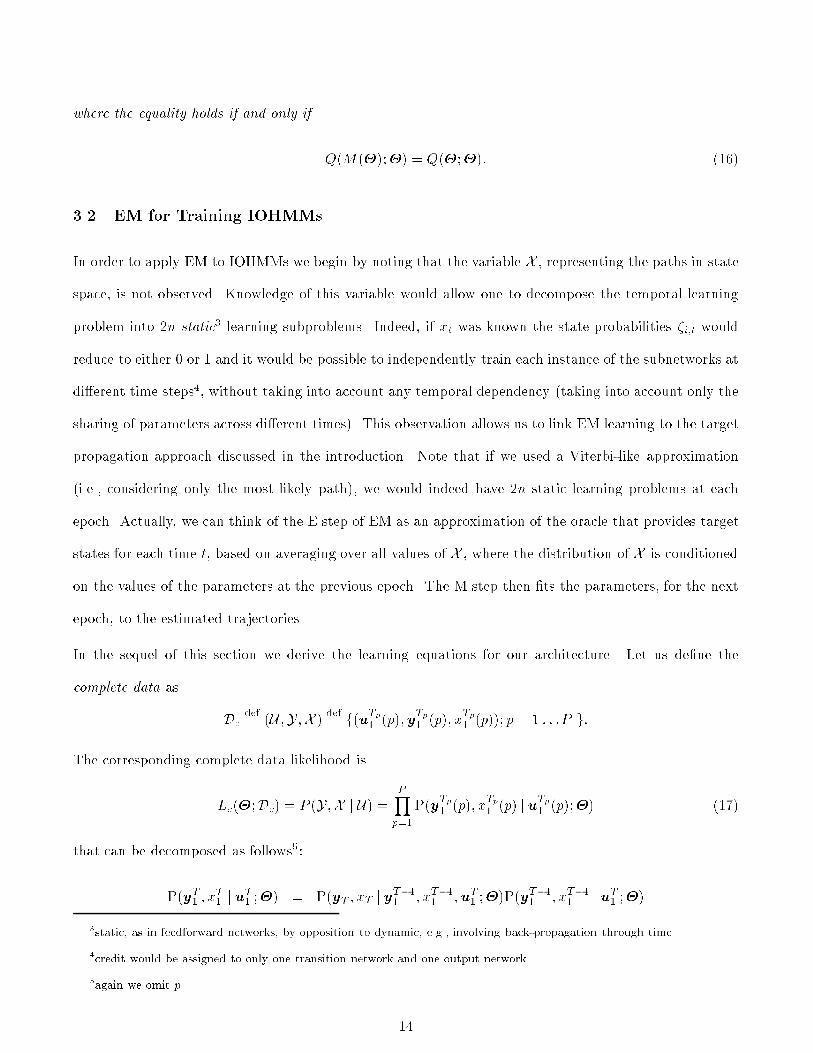
��� EM for Training IOHMMs

In order to apply EM to IOHMMs we begin by noting that the variable X � representing the paths in state

space� is not observed� Knowledge of this variable would allow one to decompose the temporal learning

problem into n static� learning subproblems� Indeed� if xt was known the state probabilities �i�t would

reduce to either � or � and it would be possible to independently train each instance of the subnetworks at

di�erent time steps�� without taking into account any temporal dependency �taking into account only the

sharing of parameters across di�erent times� This observation allows us to link EM learning to the target

propagation approach discussed in the introduction� Note that if we used a Viterbi�like approximation

�i�e�� considering only the most likely path� we would indeed have n static learning problems at each

epoch� Actually� we can think of the E step of EM as an approximation of the oracle that provides target

states for each time t� based on averaging over all values of X � where the distribution of X is conditioned

on the values of the parameters at the previous epoch� The M step then �ts the parameters� for the next

epoch� to the estimated trajectories�

In the sequel of this section we derive the learning equations for our architecture� Let us de�ne the

complete data as

Dcdef� �U �Y �X

def� f�u

Tp� �p�y

Tp� �p� x

Tp� �p� p� � � � �P g�

The corresponding complete data likelihood is

Lc���Dc � P �Y �X j U �PYp��

P�yTp� �p� x

Tp� �p ju

Tp� �p�� ���

that can be decomposed as follows�

P�yT� � xT� j u

T� �� � P�yT � xT j y

T��� � xT��� �uT� ��P�y

T��� � xT��� j uT

� ��

�static� as in feedforward networks� by opposition to dynamic� e�g�� involving back�propagation through time�

�credit would be assigned to only one transition network and one output network�

�again we omit p�

��

� P�yT � xT j xT���uT ��P�yT��� � xT��� j uT��

� ��� ���

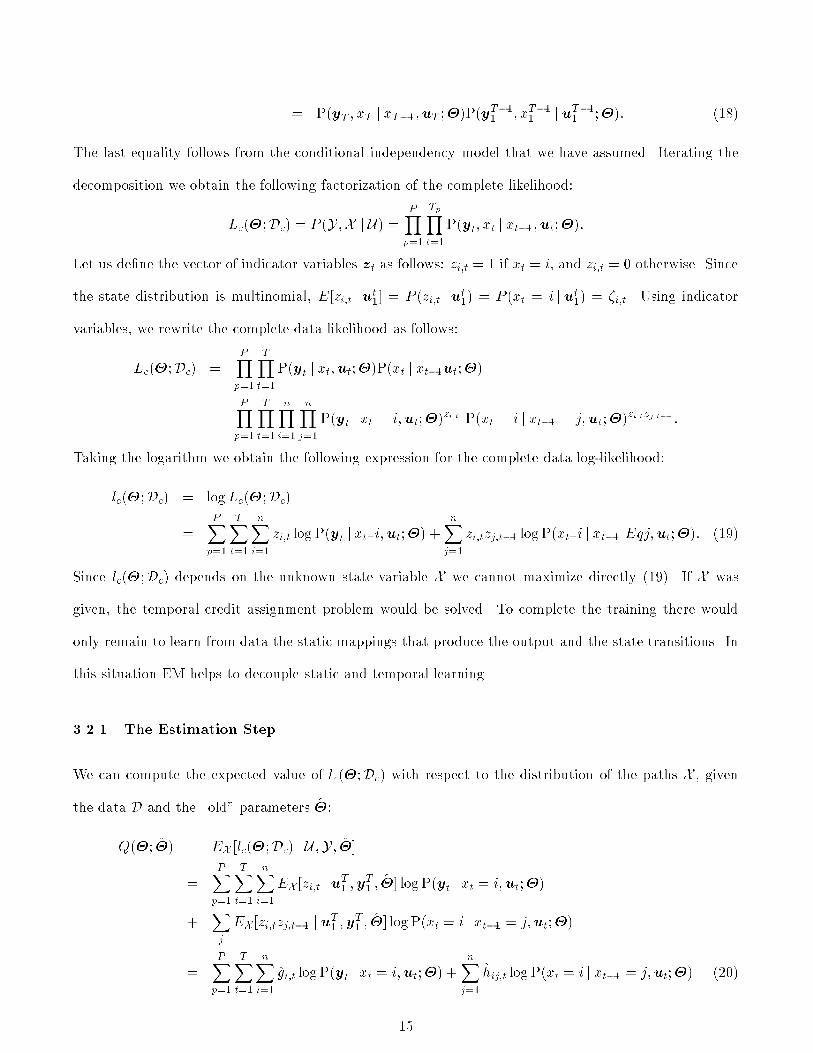
The last equality follows from the conditional independency model that we have assumed� Iterating the

decomposition we obtain the following factorization of the complete likelihood�

Lc���Dc � P �Y �X j U �PYp��

TpYt��

P�yt� xt j xt���ut���

Let us de�ne the vector of indicator variables zt as follows� zi�t � � if xt � i� and zi�t � � otherwise� Since

the state distribution is multinomial� E�zi�t j ut�� � P �zi�t jut

� � P �xt � i j ut� � �i�t� Using indicator

variables� we rewrite the complete data likelihood as follows�

Lc���Dc �PYp��

TYt��

P�yt j xt�ut��P�xt j xt��ut��

�PYp��

TYt��

nYi��

nYj��

P�yt j xt � i�ut��zi�t P�xt � i j xt�� � j�ut��

zi�tzj�t�� �

Taking the logarithm we obtain the following expression for the complete data log�likelihood�

lc���Dc � logLc���Dc

�PXp��

TXt��

nXi��

zi�t log P�yt j xt�i�ut�� �nX

j��

zi�tzj�t�� log P�xt�i j xt�� Eqj�ut��� ���

Since lc���Dc depends on the unknown state variable X we cannot maximize directly ���� If X was

given� the temporal credit assignment problem would be solved� To complete the training there would

only remain to learn from data the static mappings that produce the output and the state transitions� In

this situation EM helps to decouple static and temporal learning�

����� The Estimation Step

We can compute the expected value of lc���Dc with respect to the distribution of the paths X � given

the data D and the �old parameters ���

Q��� �� � EX �lc���Dc j U �Y � ���

�PXp��

TXt��

nXi��

EX �zi�t juT� �y

T� ���� log P�yt j xt � i�ut��

�Xj

EX �zi�tzj�t�� j uT� �y

T� ���� log P�xt � i j xt�� � j�ut��

�PXp��

TXt��

nXi��

�gi�t log P�yt j xt � i�ut�� �nX

j��

�hij�t log P�xt � i j xt�� � j�ut�� ��

��

where gi�tdef� P �xt � i j uT

� �yT� ��� and the hij�t

def� P �xt � i� xt�� � j j uT

� �yT� �� are the elements of the

autocorrelation matrix for consecutive state pairs� The hat in �gi�t and �hij�t means that these variables are

computed using the old parameters ���

In order to compute hij�t and gi�t we introduce the following probabilities� borrowing the notation from

the HMM literature�

�i�tdef� P�yt�� xt � i jut

�� ��

�i�tdef� P�yTt�� j xt � i�uTt � �

�i�t can be rewritten as follows�

�i�t � P�yt�� xt � i j ut�

�X�

P�yt�� xt � i� xt�� � � j ut�

�X�

P�yt j yt��� xt � i� xt�� � ��ut

�P�xt � i j yt��� � xt�� � ��ut�P�yt��� � xt�� � � j ut� ��

and thus� using the conditional independence assumptions graphically depicted in Figure and previously

discussed� we obtain

�i�t � P �yt j xt�i�utX�

�i��ut���t��� ��

where P �yt j xt�i�ut speci�es the output distribution in state i and �i��ut speci�es the next state

distribution in state i� both conditioned on the current input� This recursion is initialized with the initial

state probabilities �i��def� P �x� � i �which can �xed a priori or learned as extra parameters� as in HMMs�

In general� we will constrain the model to end up in one of several �nal states from the set F � so the

likelihood L���Dp for a sequence p can be written in terms of the ��s�

L � P�yT� j uT� �

Xi�F

P�yT� � xT � i j uT� �

Xi

�i�T � ��

Similarly� a backward recursion can be established for �i�t�

�i�t � P�yTt�� j xt� i�uTt

�X�

P�yTt��� xt���� j xt� i�uTt

�X�

P�yt�� j yTt��� xt����� xt� i�u

Tt P�y

Tt�� j xt����� xt� i�u

Tt P�xt���� j xt� i�u

Tt ��

��

and thus using the conditional independence assumptions�

�i�t �X�

P �yt�� j xt���l�ut��i�ut�����t��� ��

where the backward recursion is initialized with �i�T � � if i � F and � otherwise� It is maybe useful to

remark how these distributions are computed� P �yt j xt�i�ut is obtained by running subnetwork Oi on

the input vector ut� and plugging the target vector yt and Oi�s output �i�t into the algebraic expression

of the output distribution� �i��ut is simply the ��th output of subnetwork Ni� fed with the input vector

ut�

The transition posterior probabilities hij�t can be expressed in terms of � and ��

hij�t � P�xt�i� xt���j j yT�u

T�

� P�xt�i� xt���j�yT� j u

T� P�y

T� ju

T�

� P�yTt�� j xt�i� xt���j�yt��u

T� P�yt j xt�i� xt���j�y

t��� �uT� P�y

t��� � xt���j j u

T� P�xt�i j xt���j�y

t��� �uT� L

� P�ytjxt�i�ut�j�t���i�t�ij�utL ��

where the last equation is obtained using the conditional independency assumptions and L is the con�

ditional likelihood �equation �� The state posterior probabilities gi�t can be obtained by summing h�s�

withP

j hij�t� or directly�

gi�t � P�xt�i j yT�u

T�

� P�xt�i�yT� j u

T� L

� P�yTt�� j xt � i�yt��uT� P�y

t�� xt�i ju

T� L

� �i�t�i�tL ��

To summarize� we obtain equations similar to those used to train HMMs with the Baum�Welch algorithm�

A forward linear recursion �equation � can be used to compute the likelihood �equation �� During

training� a backward linear recursion �equation � is performed� that is equivalent to back�propagating

through time gradients of the likelihood with respect to the ��s ��i�t ��L��i�t

� see also ����� Notice that the

sums in equations ��� �� and �� can be constrained by the transition graph underlying the model�

��

����� The Maximization Step

Each iteration of the EM algorithm requires to maximize Q�����k�� As explained below� if the subnet�

works are linear this can be done analytically �for example with symbolic inputs� In general� however� if

the subnetworks have hidden sigmoidal units� or use a softmax function to constrain their outputs to sum

to one� the maximum of Q cannot be found analytically� In these cases we can resort to a GEM algorithm�

that simply produces an increase in Q� for example by gradient ascent� Although Theorem � guarantees

the convergence of GEM algorithms to a local maximum of the likelihood� their convergence may be

signi�cantly slower compared to EM� However� the parameterization of transition probabilities through

layers of neural units makes the learning algorithm smooth and suitable for use in on�line mode �i�e��

updating the parameters after each sequence presentation� rather than accumulating parameter change

information over the whole training set� This is a desirable property ���� and may often help to speed up

learning� Indeed� in several experiments we noticed that convergence can be accelerated using stochastic

�i�e�� on�line gradient ascent on the auxiliary function�

����� General form of the IOHMM training algorithm

In the most general form� IOHMM training can be summarized by the following algorithm�

Algorithm �

� foreach training sequence �uT��yT

�� do � Estimation step

��� foreach state j�� � � �n do

compute �ij�t� i � Sj and �j�t� by running forward the state and the output subnetworks Nj and Oj�

��� foreach i�� � � �n do

compute �i�t and �i�t �forward backward recurrences ���� and ���� using the current value � of the

parameters�

compute the posterior probabilities hij�t �for each j such that i � Sj� and gi�t �eqs� ���� and��� ���

� foreach state j�� � � �n do � Maximization step

��� adjust the parameters �j of state subnetwork Nj to maximize �or increase� for a GEM algorithm� the

functionPX

p��

TXt��

nXi��

hij�t logP �xt � i j xt���j�ut� �j��

��

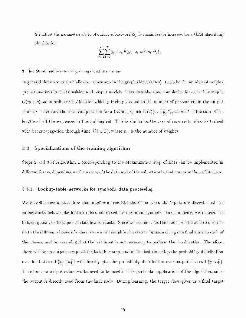
��� adjust the parameters �j to of output subnetwork Oj to maximize �or increase� for a GEM algorithm�

the functionPXp��

TXt��

gj�t logP �yt j xt � j�ut��j��

� let ��� and iterate using the updated parameters�

In general there arem � n� allowed transitions in the graph �for n states� Let p be the number of weights

�or parameters in the transition and output models� Therefore the time complexity for each time step is

O�m� p� as in ordinary HMMs �for which p is simply equal to the number of parameters in the output

models� Therefore the total computation for a training epoch is O��m� pT � where T is the sum of the

lengths of all the sequences in the training set� This is similar to the case of recurrent networks trained

with backpropagation through time� O�nwT � where nw is the number of weights�

��� Specializations of the training algorithm

Steps and � of Algorithm � �corresponding to the Maximization step of EM can be implemented in

di�erent forms� depending on the nature of the data and of the subnetworks that compose the architecture�

����� Lookuptable networks for symbolic data processing

We describe now a procedure that applies a true EM algorithm when the inputs are discrete and the

subnetworks behave like lookup tables addressed by the input symbols� For simplicity� we restrict the

following analysis to sequence classi�cation tasks� Since we assume that the model will be able to discrim�

inate the di�erent classes of sequences� we will simplify the system by associating one �nal state to each of

the classes� and by assuming that the last input is not necessary to perform the classi�cation� Therefore�

there will be no output except at the last time step� and at the last time step the probability distribution

over �nal states P�xT juT� will directly give the probability distribution over output classes P�y j u

T� �

Therefore� no output subnetworks need to be used in this particular application of the algorithm� since

the output is directly read from the �nal state� During learning� the target class gives us a �nal target

��

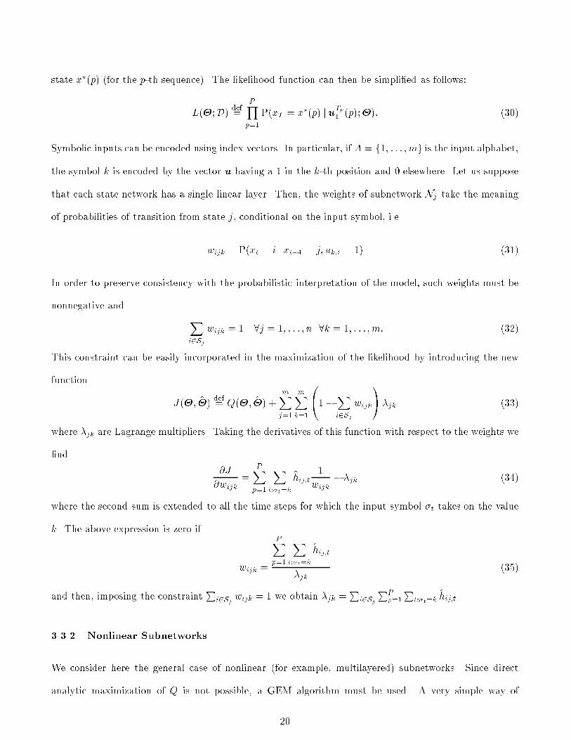
state x��p �for the p�th sequence� The likelihood function can then be simpli�ed as follows�

L���Ddef�

PYp��

P�xT � x��p juTp� �p��� ���

Symbolic inputs can be encoded using index vectors� In particular� if A � f�� � � � � mg is the input alphabet�

the symbol k is encoded by the vector u having a � in the k�th position and � elsewhere� Let us suppose

that each state network has a single linear layer� Then� the weights of subnetwork Nj take the meaning

of probabilities of transition from state j� conditional on the input symbol� i�e�

wijk � P�xt � i j xt�� � j� uk�t � � ���

In order to preserve consistency with the probabilistic interpretation of the model� such weights must be

nonnegative and

Xi�Sj

wijk � � �j � �� � � � � n �k � �� � � � � m� ��

This constraint can be easily incorporated in the maximization of the likelihood by introducing the new

function

J��� ��def� Q��� �� �

mXj��

mXk��

����

Xi�Sj

wijk

�Ajk ���

where jk are Lagrange multipliers� Taking the derivatives of this function with respect to the weights we

�nd

�J

�wijk

�PXp��

Xt�t�k

�hij�t�

wijk

� jk ���

where the second sum is extended to all the time steps for which the input symbol �t takes on the value

k� The above expression is zero if

wijk �

PXp��

Xt�t�k

�hij�t

jk���

and then� imposing the constraintP

i�Sjwijk � � we obtain jk �

Pi�Sj

PPp��

Pt�t�k

�hij�t�

����� Nonlinear Subnetworks

We consider here the general case of nonlinear �for example� multilayered subnetworks� Since direct

analytic maximization of Q is not possible� a GEM algorithm must be used� A very simple way of

�

producing an increase in Q is to use gradient ascent� The derivatives of Q with respect to the parameters

can be easily computed as follows� Let jk be a generic weight in the state subnetwork N j � From equation

�� we have

�Q��� ��

� jk�

PXp��

TpXt��

Xi�Sj

�hij�t�

�ij�t

��ij�t

� jk���

where the partial derivatives ��ij�t

��jkcan be computed using back�propagation�

Similarly� denoting with �ik a generic weight of the output subnetwork Oi� we have�

�Q��� ��

��ik�

PXp��

TpXt��

rX���

�gi�t�

��i��tlogP �yt j xt�i�ut

��i��t��ik

���

where��i��t�ik

are also computed using back�propagation� Intuitively� the parameters are updated as if the

estimation step of EM had provided soft targets for the outputs of the n subnetworks� for each time t�

� Comparisons

��� Standard Hidden Markov Models

The model proposed here is a natural extension of HMMs ��� �� �� the distribution of the output

sequence is conditioned on an input sequence� Furthermore� we propose to parameterize the next�state

and output distributions with complex modules such as arti�cial neural networks�

The most typical applications of standard HMMs are in automatic speech recognition ��� ���� In these

cases each lexical unit is associated to one model Mi� During recognition one computes for each model

the probability P�yT� jMi of having generated the observed acoustic sequence yT� � During training the

parameters are adjusted to maximize the probability that the correct model Mi generates the acoustic

observations associated to instances of the i�th lexical unit� Training is therefore not discriminant� it does

not try to learn how to decide which phoneme sequence is most likely� instead it learns �in an essentially

unsupervised way what is the distribution of observations associated to each class �e�g�� phoneme� The

likelihood of observations is maximized using the Baum�Welsh algorithm� which is an EM algorithm�

Dynamic programming techniques may be used to decode the most likely sequence of states� This most

likely state sequence can be also used during training �Viterbi algorithm to approximate the estimation

�

step of EM�

The architecture proposed in this paper di�ers from standard HMMs in two respects� computing style

and learning� With IOHMMs� sequences are processed similarly to recurrent networks� e�g�� an input

sequence can be synchronously transformed into an output sequence� This computing style is real�time

and predictions of the outputs are available as the input sequence is being processed� This architecture

thus allows us to model a transformation from an input sequence space to an output sequence space� in

this way� all the fundamental sequence processing tasks such as production� prediction� and classi�cation

can be dealt with� Finally� standard HMMs are based on a homogeneous Markov chain� whereas in

IOHMMs� transition probabilities are conditional on the input and thus depend on time� resulting in

an inhomogeneous Markov chain� Consequently� the dynamics of the system �speci�ed by the transition

probabilities are not �xed but are adapted in time depending on the input sequence�

The other fundamental di�erence is in the learning procedure� While interesting for their capabilities

of modeling sequential phenomena� a weakness of standard HMMs is their poor discrimination power

when trained by maximum likelihood estimation �MLE ����� Consider� for example� the application of

HMMs to speech recognition� In the MLE framework� each lexical unit model �corresponding to a word

or a phoneme is trained to �t the distribution of that particular unit� Each model learns from positive

examples only� without being informed by the teacher of what classes it will have to compete with� An

approach that has been found useful to improve discrimination in HMMs is based on maximum mutual

information �MMI training ����� When using MMI� the parameters for a given model are adjusted taking

into account the likelihoods of all the models and not only the likelihood of the model for the correct class

�as with the MLE criterion� It has been pointed out that supervised learning in neural networks and

discriminant learning criteria like MMI are actually strictly related ����� Unfortunately� MMI training of

standard HMMs can only be done with gradient ascent� On the other hand� for IOHMMs� the parameter

adjusting procedure is based on MLE and EM can be used� The variable yT� is used as a desired output

in response to the input uT� � resulting in more discriminant training�

Furthermore� as discussed in section �� IOHMMs are better suited for learning to represent long�term

context than HMMs �the argument hinges on the fact that IOHMMs are non�homogeneous�

Finally� it is worth mentioning that a number of hybrid approaches have been proposed to integrate

connectionist approaches into the HMM framework� For example in ���� the observations used by the

HMM are generated by a recurrent neural network� Bourlard et al� ��� ��� use a feedforward network

to estimate state probabilities� conditioned on the acoustic sequence� Instead of deriving an exact EM

or GEM algorithm� they apply Viterbi decoding in order to estimate the most likely state trajectory�

thereafter used as a target sequence for the feedforward network� A common feature of these algorithms

and the one proposed in this paper is that neural networks are used to extract temporally local information

whereas a Markovian system integrates long�term constraints� Unlike most of these systems� IOHMMs

represent a conditional distribution of a �desired output sequence when an �observed input sequence

is given� rather than being a model of some observation sequence� Furthermore �for some classes of

output and transition models� the EM algorithm can still be applied� even though IOHMMs represent a

discriminant model �whereas other hybrids of neural networks with HMMs which are discriminant can�t

be trained with the EM algorithm�

��� First and Second Order Recurrent Networks

A �rst order fully recurrent network with sigmoidal nonlinearities evolves according to the nonlinear

iterated map xt � f�Wxt�� � Vut� where xt is a continuous state vector and W and V are weight

matrices� The dynamics of an IOHMM� instead� are controlled by the recurrence �t �Pn

j�� �j�t�� �j�ut�

that updates the state distribution �t given the input sequence ut�� In the IOHMM case� the dynamics are

linear in the state variable �but nonlinear in the inputs� which may result in less general computational

capabilities� compared to recurrent networks� In order to gain some intuition about the computational

power of IOHMMs� it is useful to consider the limit case of transition probabilities that tend to � or

�� Such deterministic behavior �corresponding to equation � is obtained when the output units of the

state networks are saturated �� In this case� each state network j partitions the input space into n

regions �ij such that a transition from state j at time t � � to state i at time t occurs if and only

if ut � �ij � If multilayered state networks with enough hidden units are used� then� because of the

�In fact� the softmax function is used �eq� �� and lim���e�aiP�e�a�

equals to � if i � argmax� a� and otherwise�

�

universality results ����� the regions �ij can be arbitrarily shaped� When the output units of the state

networks are not saturated �i�e� transition probabilities are not exactly � or �� we can obtain a similar

interpretation� except that the regions �ij have soft boundaries�

Because of the multiplicative links� there are some analogies between our architecture and second order

recurrent networks that encode discrete states ����� A second order network with n state units and m

inputs evolves according to the equation

xt � f

��

nXj��

xj�t��Wjut

�A ���

whereWj � j � �� � � �n are n bym matrices of weights� An IOHMM that uses one�layered state subnetworks

would evolve� instead� with the linear recurrence

�t �nX

j��

�j�t��f �Wjut � ���

Following ����� a second order network can represent discrete states by �one�hot encoding� xi�t � � if the

state at time t is i� and xi�t � � otherwise� If these encoding assumption are satis�ed �again� this will

happen if the state units are saturated� equations �� and �� are equivalent� In second order networks

encoding discrete states� the previous state selects the weight matrix Wj to be used to predict the next

state� given the input� Thus the saturated second order network behaves like a modular architecture�

similar to the one we have described� in which distinct subnetworks are activated at time t depending on

the discrete state at time t � �� A similar interpretation of second order networks� although limited to

symbolic inputs� was proposed in �����

��� Adaptive Mixtures of Experts

Adaptive mixtures of experts �ME ��� and hierarchical mixtures of experts �HME ��� have been intro�

duced as a divide and conquer approach to supervised learning in static connectionist models� A mixture

of experts is composed by a modular set of subnetworks �experts that compete to gain responsibility in

modeling outputs in a given region of input space� The system output y is obtained as a convex combina�

tion of the experts� outputs yj � y �P

j gjyj where the weights gj are computed as a parametric function

�

of the inputs by a separate subnetwork �gating network that assigns responsibility to di�erent experts for

di�erent regions of the input space�

�t

O� O�

Network

Gating

ut

Figure �� The mixture of controllers �MC architecture �Cacciatore � Nowlan� �����

Recently� Cacciatore � Nowlan ��� have proposed a recurrent extension to the ME architecture� called

mixture of controllers �MC� in which the gating network has feedback connections� thus taking temporal

context into account� The MC architecture is shown in Figure �� The IOHMM architecture �i�e�� Figure �

can clearly be interpreted as a special case of the MC architecture� in which the gating network has a

modular structure and second order connections� In practice� Cacciatore � Nowlan used a one layer �rst�

order gating net� resulting in a model with weaker capacity� However� the more signi�cant di�erence lies

in the organization of processing� In the MC architecture modularity is exploited at the output prediction

level� whereas in IOHMMs modularity is exploited at the state prediction level as well� Another potentially

important di�erence lies in the presence of a saturating non�linearity in the recurrence loop of the MC

architecture� as in most recurrent networks� Instead� the recurrence loop of IOHMMs is purely linear�

It has been shown that such a non�linearity in the loop makes very di�cult the learning of long�term

context ���� �see next section for a discussion of learning long�term dependencies�

Learning in the MC architecture uses approximated gradient ascent to optimize the likelihood� in contrast

to the EM supervised learning algorithm proposed by Jordan � Jacobs ����� for the HME� The approx�

imation of gradient is based on one step truncated back�propagation through time �somehow similar to

Elman�s approach ���� and allows online updating for continually running sequences� which is useful for

control tasks� As shown earlier in this paper� the interpretation of the state sequences of IOHMMs as

�

missing data yields to maximization of the likelihood with an EM or a GEM algorithm�

� Learning Temporal Dependencies with IOHMMs

Generally speaking� sequential data presents long�term dependencies if the data at a given time t is

signi�cantly a�ected by the past data at times � t� Accurate modeling of such sequences is typically

di�cult� In the case of recurrent networks trained by gradient descent� credit assignment through time

is represented by a sequence of gradients of the error function with respect to the state of the sigmoidal

units� However� many researchers have found this procedure ine�ective for assigning credit over long

temporal spawns ���� ��� ���� In the case of IOHMMs trained by the EM algorithm� credit assignment

through time is represented by the sequences of posterior �i�e�� after having observed the data probabilities

P �xt�i j ut��y

t�� In the following we summarize the main results on the problem of learning long�term

dependencies with Markovian models� which include IOHMMs and HMMs� A formal analysis of this

problem can be found in �����

��� Temporal Credit Assignment

In previous work ���� we found theoretical reasons for the di�culty in training parametric non�linear

dynamical systems to capture long�term dependencies� For such systems� the dynamical evolution is

controlled by a non�linear iterated map at � M�at���ut� with at a continuous state vector� Systems

described by such an equation include most recurrent neural network architectures� The main result states

that either long�term storing or gradient propagation is harmed� depending on whether kM �k� the norm

of the Jacobian of the state transition function� is less or greater than one� If kM �k � � then the system

is endowed with robust dynamical attractors that can be used to reliably store pieces of information for

an arbitrary duration� However� gradients will vanish exponentially as they are propagated backward in

time� If kM �k � � then gradients do not vanish� but information about past inputs is gradually lost and

can be easily deleted by noisy events� For example� if element A of the system can be used to detect

particular conjunctions of inputs and state� and element B can latch that information� the problem is that

in order to train A one has to back�propagate through B� but gradients through B vanish over long time

�

periods�

In the present paper we have introduced a connectionist model whose dynamical behavior is controlled

by the constrained linear recurrence equation �t � ��ut�t��� where �t is interpreted as a probability

distribution de�ned over a set of discrete states� and ��ut corresponds to a matrix of transition proba�

bilities� In this case� the norm of the Jacobian of the state transition function is constrained to be exactly

one� Like in recurrent networks� learning in non�deterministic Markovian models generally becomes in�

creasingly di�cult as the span of the temporal dependencies increases ����� However� a very important

qualitative di�erence is that in Markovian models long�term storing and temporal credit assignment are

not necessarily incompatible� they either both occur or are both impractical� They both occur in the very

special case of an essentially deterministic model� The di�culty increases as the model becomes more

non�deterministic and is worst when it is completely ergodic� Eigenvalues of ��ut which are less than

� correspond to a loss of information about initial conditions� a di�usion of information through time�

Conversely� credit assignment backwards through time is harmed by this phenomenon of di�usion during

the backward phase �which is just the transpose of the forward phase� On the contrary� if most of the

eigenvalues of ��ut are close to one �i�e�� the models tend towards a deterministic behavior� then both

storing and credit assignment are more e�ective�

In order to provide some intuitions about the practical di�culty in learning long�term dependencies with

Markovian models� let us consider a sequence classi�cation problem with a discrete target variable y

for the last step of each training sequence� If the sequences are long and contain relevant classi�cation

information at their beginning� then clearly the task exhibits long�term dependencies� Key variables in the

temporal credit assignment problem are the probabilities �j�t of state j at time t� given the observed target

y� As shown in section �� these variables are computed during the estimation step of EM� They actually

correspond to the gradient of the likelihood with respect to the state probabilities �j�t� i�e�� they indicate

how the probabilities associated to each state at each time step should increase in order to increase the total

likelihood� We have found that in most cases the �j�t tend to become independent of j for t very far away

from the �nal supervision� Clearly� this re�ects a situation of maximum uncertainty about the changes

required to increase the likelihood� If all �j�t are the same for a given t� then all the states at this time

�

step are equally responsible for the �nal likelihood� no �small change of parameters would increase the

likelihood� This represents a serious di�culty for propagating backwards in time e�ective temporal credit

information� and makes very di�cult learning in the presence of long�term dependencies� However� when

the transition probabilities are close to � or �� long�term context can be propagated and credit assignment

through time performed correctly� Such a situation can be found for example in problems of grammar

inference in which the input�output data is essentially deterministic �as with the task studied in section ��

An analysis of this problem of credit assignment is presented in ����� in which we study the problem from a

theoretical point of view� applying established mathematical results on Markov chains ���� to the problem

of learning long term dependencies in homogeneous and non�homogeneous HMMs� Although the analysis

is the same for both ordinary HMMs and IOHMMs� there is a very important di�erence in the simplest

cure� which is to have transition probabilities near � or �� An HMM with deterministic �or almost

deterministic transition probabilities is not very useful because it can only model simple cycles� On the

other hand an IOHMM can perform a large class of interesting computations �such as grammar inference

with this same constraint� because the transition probabilities can vary at each time step depending on

the input sequence� The analyses reported in ���� also suggest that fully connected transition graphs have

the worst behavior from the point of view of temporal credit propagation� The transition graph can be

constrained using some prior knowledge on the problem� There are two main bene�ts that can be gained

by introducing prior knowledge into an adaptive model� improving generalization to new instances and

simplifying learning ���� ��� ���� Techniques for injecting prior knowledge into recurrent neural networks

have been proposed by many researchers ���� ��� ���� In these cases the domain knowledge is supposed to

be available as a collection of transition rules for a �nite automaton� A similar approach could be used

to choose good topologies of the transition graph in Markovian models �e�g�� HMMs or IOHMMs� For

example� structured left�to�right HMMs have been introduced in speech recognition with a topology that

is based on elementary considerations about speech production and the structure of language ��� ����

�

��� Reducing Credit Di�usion by Penalized Likelihood

As outlined in ����� the undesired di�usion of temporal credit depends on the fast convergence of the

rank of the product of n successive matrices of transition probabilities as n increases� The rate of rank

lossage can be reduced by controlling the norm of the eigenvalues of the transition matrices �t� The ideal

condition for credit assignment is a �!� transition matrix� whose eigenvalues are on the unitary complex

circle� Since the determinant of a matrix equals the product of its eigenvalues� a simple way to reduce the

di�usion e�ect is to add a penalty term to the log likelihood� as follows�

l���D � �PXp��

TpXt��

jdet�tj ���

where the constant � weights the in�uence of the penalty term� In this case� the maximization step of

EM will require gradient ascent �i�e�� we need to use a GEM algorithm� The contribution of the penalty

term to the gradient can be computed using the relationship

�jdet�tj

��ij�t

� jdet�tj����t

�ji� ���

We have found this �trick useful for some particularly nasty problems with very long sequences such as

the parity problem �see next section�

��� Experimental Comparisons with Recurrent Networks

We present here results on two problems for which one can control the span of input�output dependencies�

The �sequence problem and the Parity problem� These two simple benchmarks were used in ���� to

compare the long�term learning capabilities of recurrent networks trained by back�propagation and �ve

other alternative algorithms�

The �sequence problem is the following� classify a univariate input sequence� at the end of the sequence�

in one of two types� when only the �rst N elements �N � � in our experiments of this sequence carry

information about the sequence class� The sequences are constructed arti�cially by choosing a di�erent

random initial pattern for each class� Only the �nal time step in the output sequence is considered for

classifying the input sequence� Uniform noise is added to the input sequence� For the �rst � methods

�see Tables �!� we used a fully connected recurrent network with � units �with � free parameters�

�

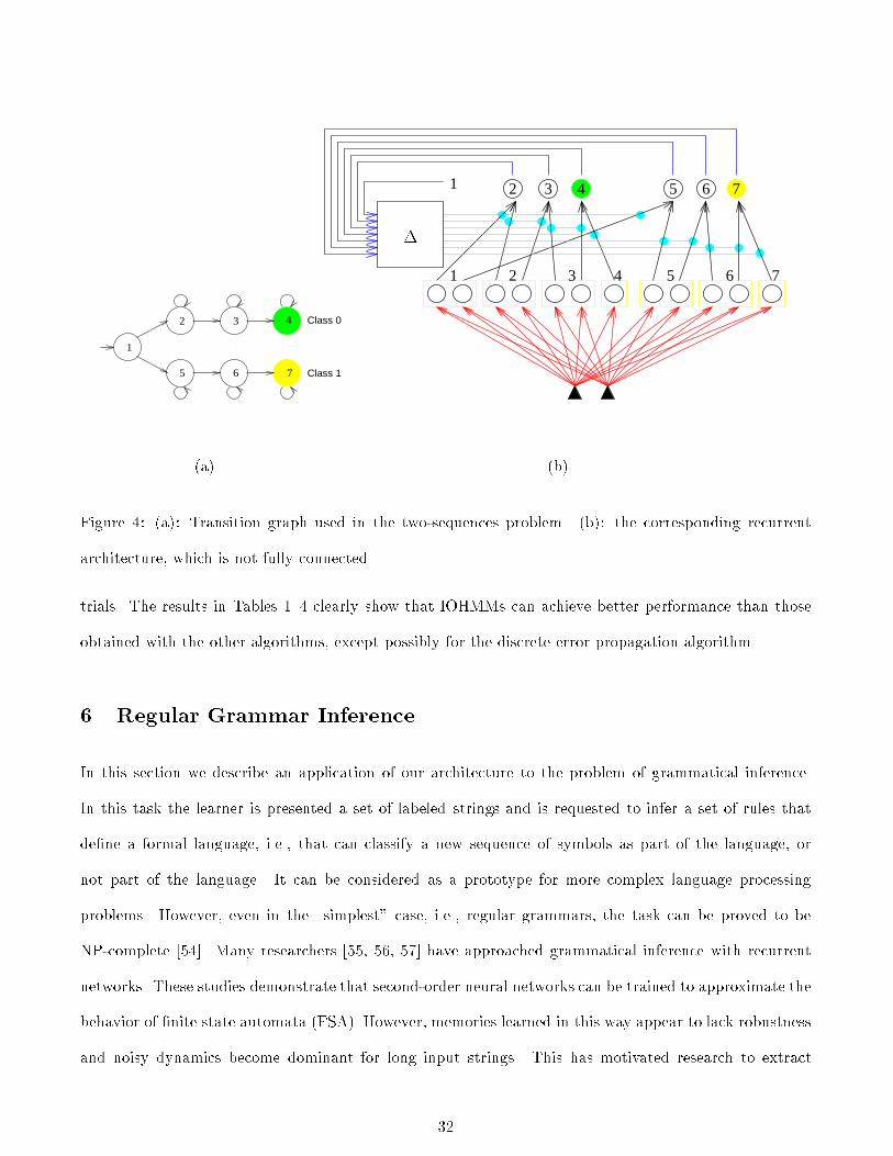
For the IOHMM� we used a ��state system with a sparse connectivity matrix �an initial state� and two

separate left�to�right sub�models of three states each to model the two types of sequences� as shown in

Figure �a� No output subnetworks are required in this case and supervision may be expressed in terms of

desired �nal state� as explained in section ������ The resulting architecture is shown in Figure �b� Other

experiments with a full transition matrix yield much worse results� although improvements were obtained

by introducing the penalty term ����

The parity problem consists in producing the parity of an input sequence of ��s and ���s �i�e�� a � should be

produced at the �nal output if and only if the number of ��s in the input is odd� The target is only given

at the end of the sequence� For the �rst � methods we used a minimal size network �� input� � hidden� �

output� � free parameters� For the IOHMM� we used a �state system with a full connectivity matrix� In

this task we found that performance could be drastically improved by using stochastic gradient ascent in

a way that helps the training algorithm get out of local optima� The learning rate is decreased when the

likelihood improves but it is increased when the likelihood remains �at �the system is stuck in a plateau

or local optimum�

For both tasks and each method� initial parameters were chosen randomly for each of � training trials�

Noise added to the input sequence was also uniformly distributed and chosen independently for each

training sequence� We considered two criteria� �� the average classi�cation error at the end of training�

i�e�� after a stopping criterion has been met �when either some allowed number of sequence presentations

has been performed or the task has been learned� � the average number of function evaluations needed

to reach the stopping criterion�

In the tables� �p�n stands for pseudo�Newton ����� Time�weighted pseudo�newton is a variation in which

derivatives with respect to the instantiation of a parameter at a particular time step are weighted by

the inverse of the corresponding second derivatives ����� Multigrid is similar to simulated annealing with

constant temperature �� The discrete error propagation algorithm ���� attempts to propagate backwards

discrete error information in a recurrent network with discrete units� Each column of the tables corresponds

to a value of the maximum sequence length T for a given set of trials� The sequence length for a particular

training sequence was picked randomly within T and T � Numbers reported are averages over � or more

��

Table �� �sequences problem� Final classi�cation error with respect to the maximum sequence length�� �� �� �� ���

back�prop �� �� �� �� ��

pseudo�newton �p�n� � � �� �� �

time�weighted p�n � � �� ��

multigrid � � � � �

discrete error prop� � �� � �� ��

simulated annealing � � � ��

IOHMMs � � � � �

Table � �sequences problem� " sequence presentations with respect to the maximum sequence length�� �� �� �� ���

back�prop �� e� ���e� �� e� ���e� ���e�

pseudo�newton �p�n� ���e� ���e� �� e� ���e� ���e�

time�weighted p�n ���e� ���e� ���e� �� e� ��e�

multigrid ���e� ���e� ���e� �� e� ���e�

discrete error prop� ���e� ���e� ���e� ���e� ���e�

simulated annealing ���e� �� e� ���e� �e� ���e�

IOHMMs ���e� ���e� �� e� ���e� �� e�

Table �� Parity problem� Final classi�cation error with respect to the maximum sequence length�� � �� �� �� ��� ���

back�prop � �� �� �� ��

pseudo�newton �p�n� � �� �� �� �� �

time�weighted p�n �� � �� ��

multigrid �� �� ��

discrete error prop� � � � �

simulated annealing � �� �

IOHMMs � � � �� � ��

Table �� Parity problem� " sequence presentations with respect to the maximum sequence length�� � �� �� ��� ���

back�prop ���e� ���e� ��e� ���e� ���e�

pseudo�newton �p�n� ���e� �� e� �� e� �e� ���e� ���e�

time�weighted p�n ���e� ��e� ���e� ���e�

multigrid ���e� ���e� ���e�

discrete error prop� ���e� � e� ���e� ���e�

simulated annealing ���e� ���e� ���e�

IOHMMs ���e� ���e� ���e� ���e� ���e� ���e�

��

Class 0

Class 1

1

2 3 4

5 6 7

1

1 2 3 4 5 6 7

432 5 6 7

�

�a �b

Figure �� �a� Transition graph used in the two�sequences problem� �b� the corresponding recurrent

architecture� which is not fully connected�

trials� The results in Tables �!� clearly show that IOHMMs can achieve better performance than those

obtained with the other algorithms� except possibly for the discrete error propagation algorithm�

� Regular Grammar Inference

In this section we describe an application of our architecture to the problem of grammatical inference�

In this task the learner is presented a set of labeled strings and is requested to infer a set of rules that

de�ne a formal language� i�e�� that can classify a new sequence of symbols as part of the language� or

not part of the language� It can be considered as a prototype for more complex language processing

problems� However� even in the �simplest case� i�e�� regular grammars� the task can be proved to be

NP�complete ����� Many researchers ���� ��� ��� have approached grammatical inference with recurrent

networks� These studies demonstrate that second�order neural networks can be trained to approximate the

behavior of �nite state automata �FSA� However� memories learned in this way appear to lack robustness

and noisy dynamics become dominant for long input strings� This has motivated research to extract

�

Table �� De�nitions of the seven Tomita grammars

Grammar De�nition

� ��

����

� string does not contain ��n����m�� as a substring� string does not contain ��� as a substring� string contains an even number of ���s and ���s� number of ��s � number of ��s is a multiple of �� ��������

automata rules from the trained network ���� ���� In many cases� it has been shown that the extracted

automaton outperforms the trained network� Although FSA extraction procedures are relatively easy

to devise for symbolic inputs� they may be more di�cult to apply in tasks involving a sub�symbolic or

continuous input space� such as in speech recognition� Moreover� the complexity of the discrete state space

produced by the FSA extraction procedure may grow intolerably if the continuous network has learned a

representation involving chaotic attractors� Other researchers have attempted to encourage a �nite�state

representation via regularization ���� or by integrating clustering techniques in the training procedure �����

We report experimental results on the application of IOHMMs to a set of regular grammars introduced by

Tomita ���� and afterwards used by other researchers as a benchmark to measure the accuracy of inference

methods based on recurrent networks ���� ��� ��� ��� ���� The grammars use the binary alphabet f�� �g

and are reported in Table �� For each grammar� Tomita also de�ned a small set of labeled strings to be

used as training data� One of the di�culties of the task is to infer the proper rules �i�e�� to attain perfect

generalization using these impoverished data�

Since the task is to classify each sequence in two classes �namely� accepted or rejected strings� we used

a scalar output and we put supervision at the last time step T � The �nal output yT was modeled as a

Bernoulli variable� i�e� P �yT � �yT

T �� � �T ��y

T � where �T is the system �nal �expected output and

the target output yT � � if the string is rejected and yT � � if it is accepted� During test we adopted

the criterion of accepting the string if �T � ���� It is worth mentioning that �nal states cannot be used

directly as targets #as done in section ��� # since there can be more than one accepting or rejecting

��

# states

Grammar #1

2 4 6

0.60

0.65

0.70

0.75

0.80

0.85

0.90

0.95

1.00

3 5 7 8

# states

Grammar #2

3 5 7

0.20

0.40

0.60

0.80

1.0

4 6 8

# states

Grammar #3

3 5 7

0.00

0.20

0.40

0.60

0.80

1.0

4 6 8

# states

Grammar #4

3 5 7

0.00

0.20

0.40

0.60

0.80

1.0

4 6 8

Figure �� Convergence and generalization attained by varying the number of discrete states n in the

model� Results are averaged over � trials� Frequency of convergence to e � � classi�cation errors on

the training set� Frequency of convergence to e � � classi�cation errors on the training set� The two

gray levels of the vertical bars show the corresponding accuracies on the test data� The triangles ��

denote the generalization accuracy for the best and the worst trial� The horizontal dashed line represents

the best result reported by Watrous � Kuhn� �continued � � ��

��

# states

Grammar #5

3 4 5 6 7 8

0.00

0.20

0.40

0.60

0.80

1.0

3 5 7 8

Ave. accuracy e<3 Ave accuracy e=0 Convergence e<3 Convergence e=0 Accuracy worst trial Accuracy best trial Watrous & Kuhn best

# states

Grammar #6

3 5 7

0.20

0.40

0.60

0.80

1.0

4 6 8

# states

Grammar #7

3 5 7

0.00

0.20

0.40

0.60

0.80

1.0

4 6 8

Figure �� �� � � continuation�

��

Table �� Summary of experimental results on the seven Tomita�s grammars �see text for explanation�

Grammar Sizes Frequency of Accuracies

n� FSA min Convergence Average Worst Best W�K Best

� � � ���� ����� ����� ����� �����

� � � ���� � �� ���� ����� �����

� � ���� ��� �� ����� ���

� � � ���� ����� ����� ����� ���

� � � ���� ����� ����� ����� ����

� � � ���� ����� ����� ����� ����

� � ���� ���� ���� ����� ���

state� In ���� this problem is circumvented by appending a special �end symbol to each string� However�

in our case this would increase the number of parameters�

The task of accepting strings can be solved by a Moore �nite state machine ����� in which the output is

function of the state only �i�e�� strings are accepted or rejected depending on what �nal state is reached�

Hence� we did not apply external inputs to the output networks� that reduced to one unit fed by a bias

input� In this way� each output network computes a constant function of the last state reached by the

model� The system output is a combination of these� weighted by �t� the state distribution at time t�

Given the absence of prior knowledge about plausible state paths� we used an ergodic transition graph in

which all transitions are allowed� Each state network was composed of a single layer of n neurons with

a softmax function at their outputs� Input symbols were encoded by two�dimensional index vectors �i�e��

ut � ��� ��� for the symbol � and ut � ��� ��� for the symbol �� The total number of free parameters is

thus n� � n�

In the experiments we measured convergence and generalization performance using di�erent sizes for the

recurrent architecture� For each setting we ran � trials with di�erent seeds for the initial weights� We

considered a trial successful if the trained network was able to correctly label all the training strings�

In order to select the model size �i�e�� the number of states n we generated a small data set composed of �

randomly selected strings of length T � �� and we applied a cross�validation criterion� For each grammar

we trained seven di�erent architectures having n � � � � � � � � and we selected the value n� that yielded the

��

best average accuracy on the cross�validation data set� Interestingly� except for grammars and �� the

same n� would have been obtained by choosing the smallest model successfully trained to correctly classify

the learning set� as shown in Figure �� This �gure shows the generalization accuracy �triangles and the

frequency of convergence to zero errors on the training set �squares� for each of the grammars� with a

comparison to the best result of � trials obtained by Watrous � Kuhn ���� with a second�order recurrent

network �dashed horizontal line on the same data� We see that most of the IOHMM trials performed

better than the best of � recurrent network trials and that the best IOHMM trial always generalized

perfectly �unlike the best recurrent network� For comparison� in Table � we also report for each grammar

the number of states of the minimal recognizing FSA �����

We tested the trained IOHMMs on a corpus of �� � � binary strings of length T � �� The �nal results

are numerically summarized in Table �� The column �Convergence reports the fraction of trials that

succeeded to separate the training set� The next three columns report averages and order statistics �worst

and best trial of the fraction of correctly classi�ed strings� measured on the successful trials� For each

grammar these results refer to the model size n� selected by cross�validation� Generalization was always

perfect on grammars ����� and �� For each grammar� the best trial also attained perfect generalization�

These results compare very favorably to those obtained with second�order networks trained by gradient

descent� when using the training sets proposed by Tomita� For comparison� in the last column of Table �

we reproduce the results reported by Watrous � Kuhn ���� in the best of �ve trials� Other researchers

also obtained interesting results� although they are not directly comparable because of the use of larger�

training sets ���� ��� or di�erent experimental conditions ����� In most of the successful trials we observed

that the model learned a �deterministic behavior� i�e�� the transition probabilities were asymptotically

converging either to � or to � �exact values of � or � would require to develop in�nite weights because

of the softmax function� Of course this is consistent with the deterministic nature of the problem� It is

however interesting to note that� apart from numerical precision problems� these trained models actually

behave like �nite automata� rendering trivial the extraction of the corresponding deterministic automaton�

Indeed� for grammars ������ and �� we found that the trained IOHMMs behave exactly like the minimal

We used the training sets dened by Tomita �� �

��

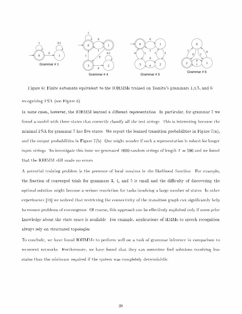
0 1

1

0

0,1

Grammar # 1

0 1

23

10 1 1

0

1

0

0

Grammar # 5

0

12

10

10

10

Grammar # 6

0 1

23

1

01

0

0,11

0

Grammar # 4

Figure �� Finite automata equivalent to the IOHMMs trained on Tomita�s grammars ������ and ��

recognizing FSA �see Figure ��

In some cases� however� the IOHMM learned a di�erent representation� In particular� for grammar � we

found a model with three states that correctly classify all the test strings� This is interesting because the

minimal FSA for grammar � has �ve states� We report the learned transition probabilities in Figure ��a�

and the output probabilities in Figure ��b� One might wonder if such a representation is robust for longer

input strings� To investigate this issue we generated ���� random strings of length T � ��� and we found

that the IOHMM still made no errors�

A potential training problem is the presence of local maxima in the likelihood function� For example�

the fraction of converged trials for grammars �� �� and � is small and the di�culty of discovering the

optimal solution might become a serious restriction for tasks involving a large number of states� In other

experiments ���� we noticed that restricting the connectivity of the transition graph can signi�cantly help

to remove problems of convergence� Of course� this approach can be e�ectively exploited only if some prior

knowledge about the state space is available� For example� applications of HMMs to speech recognition

always rely on structured topologies�

To conclude� we have found IOHMMs to perform well on a task of grammar inference in comparison to

recurrent networks� Furthermore� we have found that they can sometime �nd solutions involving less

states than the minimum required if the system was completely deterministic�

��

xt�� �t � � �t � �

�

0 1 20

.2

.4

.6

.8

1.0

0 1 20

.2

.4

.6

.8

1.0

�

0 1 20

.2

.4

.6

.8

1.0

0 1 20

.2

.4

.6

.8

1.0

0 1 20

.2

.4

.6

.8

1.0

0 1 20

.2

.4

.6

.8

1.00

12

0

.2

.4

.6

.8

1.0

�a �b

Figure �� Learned transition probabilities for grammar " �� �a� Transition probabilities� bar chart on

row j and column k represents the discrete distribution P�xt j xt�� � j� ut � k� �b� Probabilities of

accepting the input string� P �yT � � j xT � This network correctly classi�es all the test strings�

� Conclusions

We have presented a recurrent architecture suitable for modeling an input�output relationship in discrete

state dynamical systems� The architecture has a probabilistic interpretation� called Input�Output Hidden

Markov Model �IOHMM� and can be trained by an EM or GEM algorithm� using the state paths as

missing data� It can be seen both as an extension of standard Hidden Markov Models �HMMs� with

a conditioning input sequence� and as an extension of the mixture of experts �ME model ���� with a

constrained linear feedback loop and two sets of experts �for predicting the output and for predicting the

next state�

On two test problems� in which the span of the temporal dependencies can be controlled� we have found

that IOHMMs learn long�term dependencies more e�ectively than back�propagation and other alternative

algorithms described in ���� ���� An analysis of the problem of credit assignment through time in HMMs

and IOHMMs ���� explains why they could solve this problem better than recurrent networks �which

��

have a non�linearity in the recurrence loop� and revealed that best results would be obtained when

transition probabilities are near � or �� Although this corresponds to uninteresting models in the case

of HMMs� it corresponds to a large class of useful models in the case of IOHMMs� because the latter

are non�homogeneous �transition probabilities change during the sequence� Furthermore� when HMMs

are trained with the �more e�cient than gradient ascent EM algorithm they are trained in a basically

non�discriminant way� whereas IOHMMs can be trained with the EM algorithm while using a discriminant

training criterion�

The results obtained in recent experiments suggest that IOHMMs are appropriate for solving grammatical

inference problems� In particular� for the benchmark problem proposed by Tomita ����� IOHMMs compare

favorably to second order nets trained by gradient descent� in terms of generalization performance�

Future work will have to address extensions of this model in several directions� How well does the

algorithm perform on larger scale tasks with a large state space$ How can we use dynamic programming

in applications such as speech recognition where we wish to assign a certain meaning to particular states

or transitions$ How well does the algorithm work on tasks of sequence prediction �e�g� multivariate

time�series and sequence production �e�g� control and robotics tasks$ Are there other ways to improve

credit assignment through time when the data to be modeled is very non�deterministic$ We are exploring

a solution based on a hierarchical representation of the state� This can be achieved by introducing several

sub�state variables whose Cartesian product corresponds to the system state� Each of these sub�state

variables can operate at a di�erent time scale� thus allowing credit to propagate over long temporal spans

for some of these variables� A di�erent option for simplifying the sequential learning task� is to exploit

some form of prior knowledge� which can be used� not only to reduce the number of free parameters� but

also� to reduce the di�culty in capturing long�term dependencies�

References

��� A� Waibel� T� Hanazawa� G� Hinton� K� Shikano� and K� Lang� �Phoneme recognition using time�delay neural

networks�� IEEE Transactions on Acoustics� Speech� and Signal Processing� vol� �� pp� ������ � � � �

��� D� Seidl and D� Lorenz� �A structure by which a recurrent neural network can approximate a nonlinear dynamic

��

system�� in Proceedings of the International Joint Conference on Neural Networks� vol� �� pp� � ���� July

� ��

��� E� Sontag� �Systems combining linearity and saturations and relations to neural networks�� Tech� Rep� SYCON�

����� Rutgers Center for Systems and Control� � ��

��� D� Rumelhart� G� Hinton� and R�Williams� �Learning internal representations by error propagation�� in Parallel

Distributed Processing �D� Rumelhart and J� McClelland� eds��� vol� �� ch� �� pp� �������� Cambridge� MIT

Press� � ���

��� B� Pearlmutter� �Learning state space trajectories in recurrent neural networks�� Neural Computation� vol� ��

pp� ������ � � � �

��� G� Kuhn� �A �rst look at phonetic discrimination using connectionist models with recurrent links�� CCRP �

IDA SCIMP working paper No����� Institute for Defense Analysis� Princeton� NJ� � ��

�� A� Robinson and F� Fallside� �Static and dynamic error propagation networks with application to speech

coding�� in Neural Information Processing Systems �D� Anderson� ed��� �Denver� CO�� pp� �������� American

Institute of Physics� New York� � ���

��� R� Williams and D� Zipser� �A learning algorithm for continually running fully recurrent neural networks��

Neural Computation� vol� �� pp� ������� � � �

� � M� Gori� Y� Bengio� and R� De Mori� �BPS� A learning algorithm for capturing the dynamical nature of speech��

in Proceedings of the International Joint Conference on Neural Networks� �Washington D�C��� pp� ��������

IEEE� New York� � � �

���� M� Mozer� �A focused back�propagation algorithm for temporal pattern recognition�� Complex Systems� vol� ��

pp� �� ����� � � �

���� P� Frasconi� M� Gori� and G� Soda� �Local feedback multi�layered networks�� Neural Computation� vol� �� no� ��

pp� �������� � ��

���� A� Tsoi and A� Back� �Locally recurrent globally feedforward networks� a critical review of architectures�� IEEE

Transactions on Neural Networks� vol� �� no� �� pp� �� ��� � � ��

���� Y� Bengio� P� Simard� and P� Frasconi� �Learning long�term dependencies with gradient descent is di�cult��

IEEE Transactions on Neural Networks� vol� �� no� �� pp� ������� � ��

��

���� M� C� Mozer� �The induction of multiscale temporal structure�� in Advances in Neural Information Processing

Systems � �J� Moody� S� Hanson� and R� Lipmann� eds��� �San Mateo� CA�� pp� ������� Morgan Kaufmann�

� ��

���� R� Rohwer� �The time dimension of neural network models�� ACM Sigart Bulleting� vol� �� pp� ������ July

� ��

���� Y� Bengio� P� Frasconi� and P� Simard� �The problem of learning long�term dependencies in recurrent networks��

in IEEE International Conference on Neural Networks� �San Francisco�� pp� ������� �� IEEE Press� � ��

�invited paper��

��� R� Rohwer� �The �moving targets� training algorithm�� in Advances in Neural Information Processing Systems

� �D� Touretzky� ed��� �Denver� CO�� pp� �������� Morgan Kaufmann� San Mateo� � ��

���� Y� Bengio and P� Frasconi� �Credit assignment through time� Alternatives to backpropagation�� in Advances in

Neural Information Processing Systems � �J� Cowan� G� Tesauro� and J� Alspector� eds��� Morgan Kaufmann�

� ��

�� � A� P� Dempster� N� M� Laird� and D� B� Rubin� �Maximum�likelihood from incomplete data via the EM

algorithm�� Journal of Royal Statistical Society B� vol� � � pp� ����� � �

���� L� E� Baum� T� Petrie� G� Soules� and N� Weiss� �A maximization technique occuring in the statistical analysis

of probabilistic functions of Markov chains�� Ann� Math� Statistic�� vol� ��� pp� ������� � ��

���� S� Levinson� L� Rabiner� and M� Sondhi� �An introduction to the application of the theory of probabilistic

functions of a Markov process to automatic speech recognition�� Bell System Technical Journal� vol� ��� no� ��

pp� ��������� � ���

���� A� Poritz� �Hidden Markov models� a guided tour�� in Proc� Int� Conf� Acoustics� Speech� and Signal Processing�

pp� ���� � ���

���� A� Kehagias� �Stochastic recurrent networks� Prediction and classi�cation of time series�� tech� rep�� Brown

University� Division of Applied Mathematics� Providence� RI �� ��� � ��

���� H� Leprieur and P� Ha�ner� �Discriminant learning with minimum memory loss for improved non�vocabulary

rejection�� in EUROSPEECH���� �Madrid� Spain�� � ��

���� Y� Bengio� Y� LeCun� and D� Henderson� �Globally trained handwritten word recognizer using spatial repre�

sentation� space displacement neural networks and hidden Markov models�� in Advances in Neural Information

Processing Systems � �J� Cowan� G� Tesauro� and J� Alspector� eds��� pp� �� ��� � ��

�

���� G� J� McLachlan and K� E� Basford� Mixture models Inference and applications to clustering� Marcel Dekker�

� ���

��� R� A� Jacobs� M� I� Jordan� S� J� Nowlan� and G� E� Hinton� �Adaptive mixture of local experts�� Neural

Computation� vol� �� pp� ��� � ��

���� T� W� Cacciatore and S� J� Nowlan� �Mixtures of controllers for jump linear and non�linear plants�� in Advances

in Neural Information Processing Systems � �J� Cowan� G� Tesauro� and J� Alspector� eds��� �San Mateo� CA��

Morgan Kaufmann� � ��

�� � H� Bourlard and C� Wellekens� �Links between hidden Markov models and multilayer perceptrons�� IEEE

Transactions on Pattern Analysis and Machine Intelligence� vol� ��� pp� �������� � ��

���� H� Bourlard and N� Morgan� Connectionist Speech Recognition� A Hybrid Approach� vol� �� of The Kluwer

international series in engineering and computer science� Boston� Kluwer Academic Publishers� � ��

���� Y� Bengio� R� De Mori� G� Flammia� and R� Kompe� �Global optimization of a neural network�hidden Markov

model hybrid�� IEEE Transactions on Neural Networks� vol� �� no� �� pp� ������ � � ��

���� E� Levin� �Word recognition using hidden control neural architecture�� in International Conference on Acous

tics� Speech and Signal Processing� �Albuquerque� NM�� pp� �������� � ��

���� J� Bridle� �Probabilistic interpretation of feedforward classi�cation network outputs� with relationships to

statistical pattern recognition�� inNeurocomputing Algorithms� Architectures� and Applications �F� Fogelman�

Soulie and J� H�erault� eds��� New York� Springer�Verlag� � � �

���� J� Pearl� Probabilistic Reasoning in Intelligent Systems Networks of Plausible Inference� Morgan Kaufmann�

� ���

���� J� Bridle� �Training stochastic model recognition algorithms as networks can lead to maximum mutual infor�

mation estimation of parameters�� in Advances in Neural Information Processing Systems � �D� Touretzky�

ed��� pp� ������� Morgan Kaufmann� � ��

���� P� Baldi and Y� Chauvin� �Smooth on�line learning algorithms for hidden Markov models��Neural Computation�

vol� �� no� �� pp� ������� � ��

��� L� R� Rabiner� �A tutorial on hidden Markov models and selected applications in speech recognition�� Proceed

ings of the IEEE� vol� � no� �� pp� ������� � � �

��

���� P� Brown� The AcousticModeling problem in Automatic Speech Recognition� PhD thesis� Dept� of Computer

Science� Carnegie�Mellon University� � ��

�� � K� Hornik� M� Stinchcombe� and H� White� �Multilayer feedforward networks are universal approximators��

Neural Networks� vol� �� pp� �� ����� � � �

���� C� L� Giles and C� W� Omlin� �Inserting rules into recurrent neural networks�� in Neural Networks for Signal

Processing II� Proceedings of the ���� IEEE workshop �Kung� Fallside� Sorenson� and Kamm� eds��� pp� ������

IEEE Press� � ��

���� G� Z� Sun� H� H� Chen� Y� C� Lee� and C� L� Giles� �Recurrent neural networks� hidden Markov models and

stochastic grammars�� in Proc� Int� Joint Conference on Neural Networks� vol� I� �San Diego CA�� pp� � ����

� ��

���� M� I� Jordan and R� A� Jacobs� �Hierarchies of adaptive experts�� in Advances in Neural Information Processing

Systems � �J� Moody� S� Hanson� and R� Lipmann� eds��� �San Mateo� CA�� pp� ��� �� Morgan Kaufmann�

� ��

���� J� Elman� �Finding structure in time�� Cognitive Science� vol� ��� pp� � ����� � ��

���� Y� Bengio and P� Frasconi� �Di�usion of credit in markovian models�� in Advances in Neural Information Pro

cessing Systems � �G� Tesauro� D� S� Touretzky� and J� Alspector� eds��� �San Mateo� CA�� Morgan Kaufmann�

� ��

���� E� Seneta� Nonnegative Matrices and Markov Chains� New York� Springer� � ���

���� Y� S� Abu�Mostafa� �Learning from hints in neural networks�� Journal of Complexity� vol� �� pp� � ��� �� � ��

��� G� G� Towell� J� W� Shavlik� and M� O� Noordewier� �Re�nement of approximate domain theories by knowledge�

based neural networks�� in Proceedings of the Eighth National Conference on Arti cial Intelligence� �Boston�

MA�� pp� �������� � ��

���� V� Tresp� J� Hollatz� and S� Ahmad� �Network structuring and training using rule�based knowledge�� in Ad

vances in Neural Information Processing Systems � �S� J� Hanson� J� D� Cowan� and C� L� Giles� eds��� San

Mateo� CA� Morgan Kaufman Publishers� � ��

�� � C� W� Omlin and C� L� Giles� �Training second�order recurrent neural networks using hints�� in Machine

Learning Proc� of the Ninth Int� Conference �D� Sleeman and P� Edwards� eds��� �San Mateo CA�� Morgan

Kaufmann� � ��

��

���� R� Maclin and J� W� Shawlik� �Re�ning domain theories expressed as �nite�state automata�� in Machine

Learning Proceedings of the Eighth International Workshop �L� Birnbaum and G� Collins� eds��� �San Mateo

CA�� Morgan Kaufmann� � ��

���� P� Frasconi� M� Gori� M� Maggini� and G� Soda� �Uni�ed integration of explicit rules and learning by example

in recurrent networks�� IEEE Transactions on Knowledge and Data Engineering� vol� � no� �� pp� ��������

� �� �in press��

���� R� Bakis� �Continuous speech recognition via centisecond acoustic states�� in ��st Meeting of the Acoustic

Society of America� April � ��

���� S� Becker and Y� LeCun� �Improving the convergence of back�propagation learning with second order methods��

in Proceedings of the ���� Connectionist Models Summer School �D� Touretzky� G� Hinton� and T� Sejnowski�

eds��� �Pittsburg � ���� pp� � ��� Morgan Kaufmann� San Mateo� � � �

���� D� Angluin and C� Smith� �Inductive inference� Theory and methods�� Computing Surveys� vol� ��� no� ��

pp� ����� � � ���

���� C� L� Giles� C� B� Miller� D� Chen� H� H� Chen� G� Z� Sun� and Y� C� Lee� �Learning and extracted �nite state

automata with second�order recurrent neural networks�� Neural Computation� vol� �� no� �� pp� � ������ � ��

���� J� B� Pollack� �The induction of dynamical recognizers�� Machine Learning� vol� � no� �� pp� � ����� � ��

��� R� L� Watrous and G� M� Kuhn� �Induction of �nite�state languages using second�order recurrent networks��

Neural Computation� vol� �� no� �� pp� �������� � ��

���� M� Gori� M� Maggini� and G� Soda� �Insertion of �nite state automata into recurrent radial basis function

networks�� Tech� Rep� DSI��� �� Universit�a di Firenze �Italy�� � �� �submitted��

�� � S� Das and M� C� Mozer� �A uni�ed gradient�descent�clustering architecture for �nite state machine induction��

in Advances in Neural Information Processing Systems � �J� Cowan� G� Tesauro� and J� Alspector� eds��� Morgan

Kaufmann� � ��

���� M� Tomita� �Dynamic construction of �nite�state automata from examples using hill�climbing�� in Proceedings

of the Fourth Annual Cognitive Science Conference� �Ann Arbor� MI�� pp� �������� � ���

���� J� E� Hopcroft and J� D� Ullman� Introduction to Automata Theory� Languages� and Computation� Reading�

MA� Addison�Wesley Publishing Company� Inc�� � �

��