STATE-BASED GAUSSIAN SELECTION IN LARGEVOCABULARY CONTINUOUS SPEECHRECOGNITION USING HMMSM.J.F.Gales1, K.M.Knill2 & S.J.YoungJanuary 1997 (revised January 1998)EDICS Number: SA 1.6.10Cambridge University Engineering Department,Trumpington Street, Cambridge CB2 1PZ, EnglandEmail: mjfg@watson.ibm.com, kmk@nuance.com, sjy@eng.cam.ac.ukAbstractThis paper investigates the use of Gaussian Selection (GS) to increase the speed of alarge vocabulary speech recognition system. Typically 30-70% of the computational time of acontinuous density HMM-based speech recogniser is spent calculating probabilities. The aimof GS is to reduce this load by selecting the subset of Gaussian component likelihoods thatshould be computed given a particular input vector. This paper examines new techniques forobtaining \good" Gaussian subsets or \shortlists". All the new schemes make use of stateinformation, speci�cally which state each of the Gaussian components belongs to. In this waya maximum number of Gaussian components per state may be speci�ed, hence reducing thesize of the shortlist. The �rst technique introduced is a simple extension of the standard GSmethod, which uses this state information. Then, more complex schemes based on maximisingthe likelihood of the training data are proposed. These new approaches are compared withthe standard GS scheme on a large vocabulary speech recognition task. On this task, theuse of state information reduced the percentage of Gaussians computed to 10-15%, comparedwith 20-30% for the standard GS scheme, with little degradation in performance.1M.J.F.Gales is now at the IBM T.J. Watson Research Center, Yorktown Heights, NY 10598, USA.2K.M. Knill is now at Nuance Communications, 1380 Willow Rd, Menlo Park, CA 94025, USA.

List of Tables1 Change in the average forced alignment likelihood of the ARPA 1994 H1 de-velopment data for SGS and SBGS systems, compared to the standard no GSsystem. . . . . . . . . . . . . . . . . . . . . . . . . . . . . . . . . . . . . . . . . 212 Recognition performance of the standard no GS, SGS and SBGS systems onthe ARPA 1994 H1 task. . . . . . . . . . . . . . . . . . . . . . . . . . . . . . . . 213 The percentage of states assigned at each context level in MLGS and OGS.�(d) is the context dependent level, �(i) is the context independent level and�(�) is cluster level, with � = 1:9. . . . . . . . . . . . . . . . . . . . . . . . . . . 224 Change in the average forced alignment likelihood of the ARPA 1994 H1 de-velopment data for MLGS and OGS with li = 50, compared to the standardno GS system. . . . . . . . . . . . . . . . . . . . . . . . . . . . . . . . . . . . . 225 Recognition performance of MLGS and OGS on the ARPA 1994 H1 task withN1 = 6, N3 = 1 and � = 1:9. . . . . . . . . . . . . . . . . . . . . . . . . . . . . 226 Summary of comparative performance for the various selection schemes on theARPA 1994 H1 Task. . . . . . . . . . . . . . . . . . . . . . . . . . . . . . . . . . 23

2

1 IntroductionHigh accuracy large vocabulary continuous speech recognition (LVCSR) HMM-based systems havebeen developed in recent years. These systems tend to operate at several times real-time whichis not practical for most applications. Techniques are therefore required to reduce the decodingtime to faster than real-time, while maintaining, or staying close to, the same level of accuracy.To obtain a high level of accuracy, LVCSR HMM-based systems typically use continuous densityHMMs (CDHMMs). In such systems, calculation of the state likelihoods makes up a signi�cantproportion (between 30 to 70%) of the computational load. This is a result of the need to usemultiple mixture Gaussian output distributions in a state. Anywhere from 8 to 64 Gaussiancomponents are typically used and each Gaussian component must be separately evaluated inorder to determine the overall likelihood. A wide variety of techniques may be used to reducethe amount of computation required. Most of these techniques involve alteration of the acousticfeature vector and/or the acoustic models from the full CDHMM system. For example, lineardiscriminant analysis [Hunt and Lefebre, 1989] can be used to reduce the number of elements inthe feature vector, or the Gaussian components may be more tightly \tied" as in a semi-continuousHMM system [Huang et al., 1990]. The problem with these techniques is that, in the majority ofcases, these modi�cations lead to a degradation in performance. An alternative approach is to useGaussian Selection (GS) [Bocchieri, 1993]. GS methods reduce the likelihood computation of asystem by only computing the likelihood of a selected subset, or \shortlist" [Murveit et al., 1994],of Gaussian components at each frame. The underlying system remains unchanged. This paperpresents techniques to optimise the selection of the shortlists within the GS framework to minimisethe likelihood computation without degrading recognition accuracy.The motivation behind GS is as follows. If an input vector is an outlier with respect to aGaussian component distribution, i.e. it lies on the tail of the distribution, then the likelihood ofthat Gaussian component producing the input vector is very small. This results in the likelihoodof the input frame per Gaussian component within a state having a large dynamic range, withone or two Gaussian components tending to dominate the state likelihood for a particular inputvector. Hence, the state likelihood could be computed solely from these Gaussian componentswithout a noticeable loss in accuracy. GS methods attempt to e�ciently select these Gaussiancomponents, or a subset containing them, for each input vector. A number of di�erent methodshave been proposed which can be classi�ed in terms of their approach to partitioning the acousticspace, including; vector quantisation (VQ) [Bocchieri, 1993, Murveit et al., 1994], binary searchtrees [Fritsch and Rogina, 1996], dynamic searches [Beyerlein, 1994, Beyerlein and Ullrich, 1995]or a combination of these [Ortmanns et al., 1997].This paper addresses the question of how to select the \best" shortlist given a division of acous-tic space. The best shortlist can be de�ned as the one that minimises the likelihood computation1

for no, or minimal, loss in recognition accuracy. This work was based on the original GS schemeproposed by Bocchieri [Bocchieri, 1993]. However, it is directly applicable to any VQ-based GSscheme and similar methods may be applied to any static GS approach. The range of GS tech-niques is described in section 2. Section 3 reviews the standard GS scheme of Bocchieri, howthe Gaussian codewords are generated and how performance is assessed. The following sectiondescribes how state information may be incorporated into the selection process. Section 5 detailsa re�nement of this based on a maximum likelihood approach to GS. These schemes are evaluatedon a standard large vocabulary speech recognition task, the unlimited vocabulary Hub 1 task fromthe 1994 ARPA evaluation [Pallett et al., 1995].2 Gaussian Selection TechniquesIn the original implementation of GS by Bocchieri [Bocchieri, 1993] the acoustic space is divided upduring training into a set of vector quantised regions. Each Gaussian component is then assignedto one or more VQ codewords. The subset of Gaussians linked to a codeword is commonly calledthe shortlist [Murveit et al., 1994]. During recognition, the input speech vector is vector quantised,that is the vector is mapped to a single VQ codeword. The likelihood of each Gaussian componentin this codeword's shortlist is computed exactly. For the remaining Gaussian components, thelikelihood is approximated. The VQ codebooks can be generated by clustering either the Gaussiancomponents [Bocchieri, 1993] or training data [Murveit et al., 1994].Alternatively acoustic space can be partitioned by building binary search trees and assigningGaussian components relative to the tree nodes. One such technique is the Bucket Box Intersection(BBI) [Fritsch and Rogina, 1996]. In each dimension of acoustic space there is a region wherethe log probability of a Gaussian component exceeds some threshold. The regions associatedwith a particular Gaussian component are enclosed within a K-dimensional box. This allowsrapid partitioning of the acoustic space. The acoustic space is partitioned by building a K-d (Kdimensions, depth d) binary tree. This produces 2d disjoint rectangular regions (buckets). Thetree is built so that the splits between regions minimise the number of bucket-box intersections.In recognition, an input vector can be assigned to a unique bucket by descending the tree. OnlyGaussians whose box's intersect with the current bucket are computed. Multiple trees are builtfor di�erent groups of Gaussian components. This type of scheme is best suited to systems witha large number of Gaussian components per state (or mixture).If the HMM system has a single shared covariance then fast dynamic searches can be imple-mented during recognition to determine which Gaussian components are close to the input vector 3.3On-line distance metric based searches are not suited to systems without a shared covariance as the computationrequired to perform the search is close to the full likelihood computation.2

Fast nearest neighbour searches take advantage of the fact that Gaussian components can be elim-inated from likelihood computation based on a partial or relative (to other Gaussian components)distance. The exact distance between the Gaussian component and the input vector thereforedoes not have to be computed so approximations can be used in the search. For example theRecall-Jump-Eliminate and partial-distance algorithms [Beyerlein, 1994] and the Hamming dis-tance approximation [Beyerlein and Ullrich, 1995]. Alternatively, a tree can be built dynamicallysuch as in the projection search algorithm (PSA) [Ortmanns et al., 1997]. In the PSA, acousticspace is gradually partitioned to leave a small hypercube centered around the input vector. Thenumber of Gaussian component likelihoods to be fully evaluated is reduced at each partition byeliminating the Gaussian components that lie outside the new hypercube. Unlike the K-d tree,a dimension may be revisited. These techniques can be combined with each other or with VQshortlists [Ortmanns et al., 1997].3 VQ-Based Gaussian SelectionThe �rst task in VQ-based Gaussian selection is to generate a set of codewords, or clusters. Eachcodeword is then assigned a shortlist of Gaussians. When an input vector is mapped to a codewordduring recognition, the likelihood of each Gaussian in the associated shortlist is computed. Thedecrease in computational load is dependent on the size of this shortlist.3.1 Gaussian Cluster GenerationFor the work presented here a single codebook was used. The codewords were generated byclustering Gaussians during training as follows. A weighted Euclidean distance between the meanswas used to calculate the distance between the ith and jth Gaussians.�(�i; �j) = 1K KXk=1 fw(k)(�i(k)� �j(k))g2 (1)where K is the feature vector dimension, �i(k) is the kth component of vector �i, and w(k)is equal to the inverse square root of the kth diagonal element of the average of the covari-ances of the Gaussian set N (�m;�m);m = 1; : : : ;M , where �m is the diagonal covariance of themth Gaussian component. Using this metric, a clustering procedure based on the Linde-Buzo-Gray [Linde et al., 1980] algorithm was applied to minimise the average (per Gaussian component)distortion, �avg , �avg = 1M MXm=1� �min�=1 �(�m; c�)� (2)3

where M is the number of Gaussian components in the model set, � is the number of clusters(pre-de�ned), and c� is the centre (codeword) of the �th cluster ��,c� = 1size(��) Xm2�� �m; � = 1; : : : ;� (3)In all schemes, it is necessary to assign each observation vector (i.e. speech input vector)to one of the clusters during recognition in order to select the Gaussian shortlist to evaluate.The appropriate cluster is selected by determining the cluster centroid, c�, which minimises theweighted Euclidean distance to the observation vector, o(t), at time t,�t = argmin�� �(o(t); c�) (4)In some of the Gaussian selection schemes proposed here it is also necessary to assign the trainingdata to one of the clusters. Although the same cluster selection scheme may be used, there isalso the option of using a softmax assignment. Hence for generality when describing the variousGaussian selection schemes, the cluster selection will be described in terms of a \probability",p(��jo(t)). However, in all experiments described in this work a hard assignment as determinedby equation 4 was actually used.3.2 Standard Gaussian SelectionIf a Gaussian shortlist for cluster ��, ��, was generated solely from the Gaussians used in thecluster generation, the clusters would be disjoint. When used in recognition, errors would then belikely since the likelihood of some Gaussians close to the input feature vector but not in the selectedcluster would be excluded from the full computation. To avoid this, clusters share Gaussians asfollows. Given a threshold � � 0, an input feature vector, o, is said to fall on the tail of the mthGaussian if 1K KXk=1 (o(k)� �m(k))2�2m(k) � 1 (5)where �2m(k) is the ith diagonal element of�m. Thus, if the cluster centroid is taken to be a typicalinput feature vector, the Gaussian shortlist, ��, of codeword ��, can be de�ned as consisting ofall Gaussians such that [Bocchieri, 1993]G(m) 2 �� i� 1K KXk=1 (c�(k)� �m(k))2�2avg(k) � � (6)where �2avg(i) is the ith diagonal element of the matrix of the average covariance of all Gaussiansin the HMM set and G(m) indicates Gaussian component m of the standard recognition system.An alternative method for determining which Gaussians are to be in the shortlist is to useG(m) 2 �� i� 1K KXk=1 (c�(k)� �m(k))2q(�2avg(k)�2m(k)) � � (7)The advantage of this measure is that Gaussian components with large variances are encouraged4

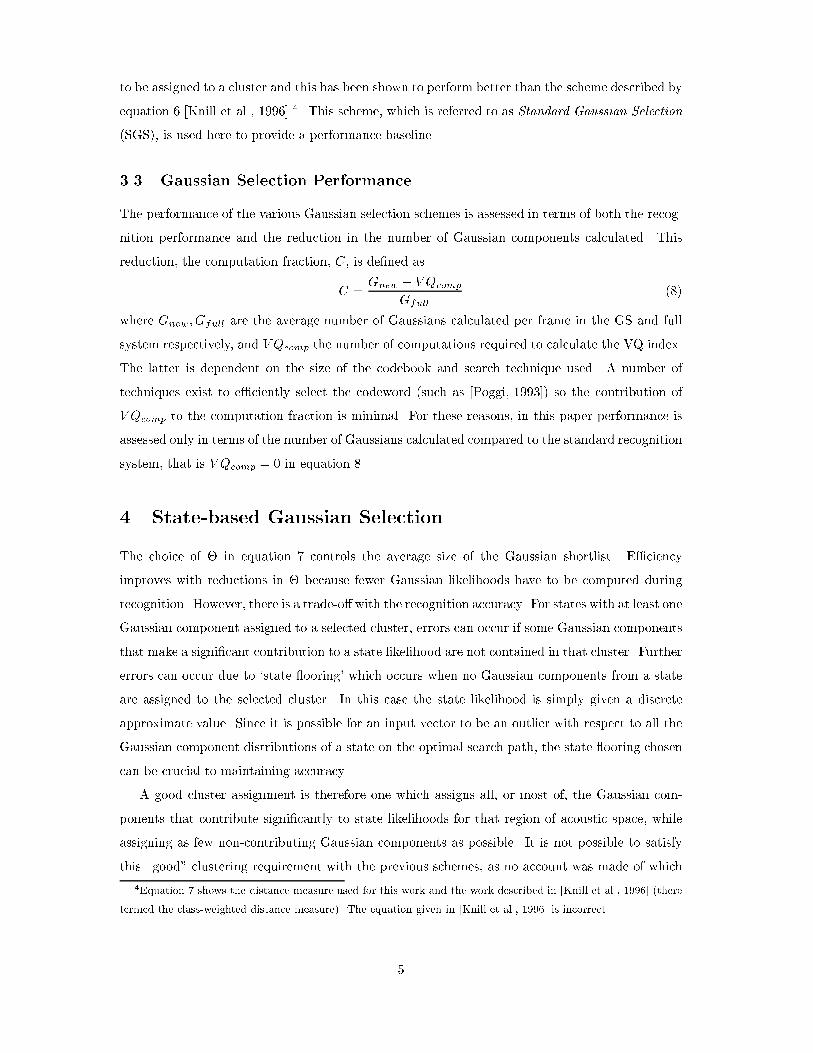
to be assigned to a cluster and this has been shown to perform better than the scheme described byequation 6 [Knill et al., 1996] 4. This scheme, which is referred to as Standard Gaussian Selection(SGS), is used here to provide a performance baseline.3.3 Gaussian Selection PerformanceThe performance of the various Gaussian selection schemes is assessed in terms of both the recog-nition performance and the reduction in the number of Gaussian components calculated. Thisreduction, the computation fraction, C, is de�ned asC = Gnew + V QcompGfull (8)where Gnew ; Gfull are the average number of Gaussians calculated per frame in the GS and fullsystem respectively, and V Qcomp the number of computations required to calculate the VQ index.The latter is dependent on the size of the codebook and search technique used. A number oftechniques exist to e�ciently select the codeword (such as [Poggi, 1993]) so the contribution ofV Qcomp to the computation fraction is minimal. For these reasons, in this paper performance isassessed only in terms of the number of Gaussians calculated compared to the standard recognitionsystem, that is V Qcomp = 0 in equation 8.4 State-based Gaussian SelectionThe choice of � in equation 7 controls the average size of the Gaussian shortlist. E�ciencyimproves with reductions in � because fewer Gaussian likelihoods have to be computed duringrecognition. However, there is a trade-o� with the recognition accuracy. For states with at least oneGaussian component assigned to a selected cluster, errors can occur if some Gaussian componentsthat make a signi�cant contribution to a state likelihood are not contained in that cluster. Furthererrors can occur due to `state ooring' which occurs when no Gaussian components from a stateare assigned to the selected cluster. In this case the state likelihood is simply given a discreteapproximate value. Since it is possible for an input vector to be an outlier with respect to all theGaussian component distributions of a state on the optimal search path, the state ooring chosencan be crucial to maintaining accuracy.A good cluster assignment is therefore one which assigns all, or most of, the Gaussian com-ponents that contribute signi�cantly to state likelihoods for that region of acoustic space, whileassigning as few non-contributing Gaussian components as possible. It is not possible to satisfythis \good" clustering requirement with the previous schemes, as no account was made of which4Equation 7 shows the distance measure used for this work and the work described in [Knill et al., 1996] (theretermed the class-weighted distance measure). The equation given in [Knill et al., 1996] is incorrect.5

state the Gaussian component belonged to. The concept of retaining the Gaussian componentto state information is therefore introduced (based on preliminary work in [Knill et al., 1996]).This scheme will be referred to as State-Based Gaussian Selection (SBGS). SBGS allows a maxi-mum number of Gaussian components associated with each state to be de�ned using the followingselection routine G(jm) 2 �� i� G(jm) 2 argminm (n) fD(G(jm); c�)g (9)whereG(jm) is the Gaussian componentm of state j, D(G(jm); c�) represents the \distance" fromG(jm) to the cluster centroid c� and for this work is the same measure as used in equation 7,and argminm(n)fg represents selecting the minimum n Gaussian components according to theselected distance measure. There is also an added constraint that D(G(jm); c�) � �.The state-based selection process can be further re�ned if the following assumption is made.That is, the Gaussian components closest to the cluster centroid are more likely to produce thedata that will be mapped to that codeword. Under this assumption, those states with Gaussiancomponents near to the centre of the cluster should be modelled more accurately by assigningmore Gaussian components from these states. This is essentially equivalent to assigning moreGaussian components from states which are often seen in the training data for that codeword andfewer to those seen less. This requirement is most easily achieved using a \multi-ring" approach.In this approach, two extra thresholds are applied, �1, �2, where �1 < �2 � �. If the distanceof the closest Gaussian component of state j to the cluster centroid c� is less than �1 then themaximum number of Gaussian components in the shortlist associated with that state is set to N1.The second threshold �2 is then used to give a maximum number of Gaussian components forstates whose closest Gaussian component falls between �1 and �2. This is simply described by thefollowing algorithm for selecting the maximum number of Gaussian components n in equation 9if (minm fD(G(jm); c�)g � �1) thenn = N1else if (minm fD(G(jm); c�)g � �2) thenn = N2else n = 0where N1 � N2 � 0, with the constraint throughout that for all selected Gaussian componentsD(G(jm); c�) � �. Thus �2 controls which states are to be \ oored" and �1 controls whichstates are more accurately modelled. This is a simple two-ring approach, though of course morecomplex functions may be used.6

5 Maximum Likelihood Gaussian Selection5.1 Selection ProcessGaussian selection aims to select the set of Gaussians that will best model the data that will beassigned to a particular cluster during recognition. The GS techniques described above base thisselection purely on distance from the cluster centroid. This is clearly sub-optimal since it requirestwo crude assumptions to be made. First, the centroid is assumed to be representative of theacoustic realisations of each Gaussian associated with that cluster. However, since Gaussians frommany di�erent phonetic contexts will usually be assigned to the same cluster, the associated dataframes may di�er substantially. Thus, the cluster centroid may be a poor representation of thedata from a particular context. Second, the choice of Gaussians takes no account of their abilityto model the data. For example the actual distribution may be bimodal, with one peak near thecenter of the cluster and the second further out. Simply choosing the closest Gaussian componentsto the cluster center will not well model the data in this case.To overcome these problems an alternative scheme, Maximum Likelihood Gaussian Selection(MLGS) is proposed. The aim of this scheme is to select the set of Gaussians that minimise thedi�erence in likelihood of the training data between the standard and Gaussian selected systems5.Thus, the Gaussian shortlist for state j and cluster ��, �̂�, is selected according to�̂� = argmin�� 8<: TXt=1 j(t)p(��jo(t)) log0@ MjXm=1wjmN (o(t);�jm;�jm)1A �TXt=1 j(t)p(��jo(t)) log0@ XG(jm)2�� wjmN (o(t);�jm;�jm)1A9=; (10)where Mj is the number of Gaussian components in state j and the state occupation probability j(t) is given by j(t) = p(qj(t)jOT ) (11)where qj(t) denotes the occupation of state j at time t. This probability is computed from thesystem with no GS. Hence the basic criterion for selecting Gaussian components for the shortlistis to choose the set that minimises the loss in likelihood between the standard no GS system andthe new GS system with the assumption that the frame-state alignments do not signi�cantly alter.Given that Gaussian components may only be left out, the Gaussian shortlist that maximisesthe probability of the training data, will be the one that minimises equation 106. To �nd the\true" best set of Gaussian components requires checking through all possible combinations of therequired number of Gaussians. The ordering of the groups of Gaussian components is then based5These are not really likelihoods, but auxiliary function values. It is therefore assumed for this work that theframe-state alignment will be the same for both the full and Gaussian selected scheme.6This assumes that a well trained initial model set is used.7

on the likelihood scores. This may be done, but for many systems quickly becomes impractical7.Appendix A describes an algorithm which closely approximates this desired scheme.For practical applications, however, a simpler implementation strategy is desirable. If it isassumed that for a state-cluster pairing, the associated data is well modelled by the n Gaussiancomponents from that state with the highest likelihood, then the selection process becomesG(jm) 2 �� i� G(jm) 2 argmaxm (n)( TXt=1 j(t)p(��jo(t)) log �wjmN (o(t);�jm;�jm)�) (12)Although this approximate scheme is only guaranteed to yield the maximum likelihood solutionwhen a single Gaussian component is to be selected, it is computationally very e�cient. It alsorequires relatively little memory, since it is only necessary to store the probability of the state-cluster pairing for each Gaussian component-cluster pairing. It is this implementation of maximumlikelihood GS that is used in this work and is referred to as MLGS.A simple alternative scheme, not based on likelihoods, which attempts to improve the modellingof the data from the state-cluster pairing is to use the occupancy counts. HereG(jm) 2 �� i� G(jm) 2 argmaxm (n)( TXt=1 jm(t)p(��jo(t))) (13)where the component occupation probability jm(t) is given by jm(t) = p(qjm(t)joT ) (14)and qjm(t) indicates \being in" Gaussian component m of state j at time t. Again this probabilityis calculated using the standard, no GS, system. This selects the set of Gaussian components withthe greatest occupancy for that cluster-state pairing. The example of bimodal distributions istherefore well handled as the Gaussian components \nearest" the two maxima should have higheroccupancy counts. Unfortunately in this scheme the data from Gaussian components with lowoccupancy counts is completely ignored when selecting the Gaussian components for the shortlist.This will be referred to as Occupancy Gaussian Selection (OGS).5.2 Handling Limited Training DataIt has so far been implicitly assumed that there is an in�nite amount of training data. Thus allstate-cluster pairs that will ever be feasible will have non-zero occupancies. Of course in realitythis is not the case. For most large vocabulary systems the number of Gaussian components andstates is selected to make best use of the available training data. It is therefore very unlikely thatall feasible pairings will be observed. However what can be stated is that the most likely pairingsare liable to occur in the training data.7Suppose that 4 Gaussian components are to be selected from each 12 Gaussian component state. In this case,there are 495 ( 12!4!8! ) combinations to consider for each state-cluster pairing. This also assumes that it is knowna-priori the number of Gaussian components required for the particular pairing.8

In most systems the vast majority of the occupancies for these state-cluster pairings will bezero. Additionally many of the remaining pairings will have very low counts making them verypoor estimates of the true8 data associated with the state-cluster pairing. Hence basing a selectionprocess on such state-cluster pairings may result in a \poor" shortlist. However the problem ofrobust estimates is a standard one in speech recognition. Many of the standard techniques used forrobustly building large vocabulary systems may be used here, for example appendix B describeshow decision trees may be used for this task.In the work presented here, however, a simple backing-o� scheme is used whereby each state-cluster pairing is only used without any modi�cation if there is \su�cient data". At this mostspeci�c level, the context-dependent level, the determination of \su�cient data" is simply based ona minimum occupancy measure, ld. For those states exceeding this threshold the selection processis the same as equation 12. Unfortunately many state-cluster pairings will have low occupancycounts and for these pairings it is necessary to back-o� to the context-independent level. If allcontexts of each phone have the same HMM topology, then each state may be separately consideredat the context-independent level. For MLGS with backo�, the shortlist selection function de�nedby equation 12 is thus modi�ed as followsG(jm) 2 �� i� G(jm) 2 argmaxm (n)8<: Xk2s(j) TXt=1 k(t)p(��jo(t)) log �wjmN (o(t);�jm;�jm)�9=;(15)where s(j) indicates the list of all states associated with the same monophone as state j and in thesame state position. Again a minimum occupancy threshold, li, may be used to determine whetherthere is su�cient data at this stage. If there is still insu�cient data it is necessary to back-o� tothe cluster level. Here all data associated with a particular cluster is used in the selection process.At this stage there is little useful temporal information in the state position, so all the states arecombined together. The selection process now becomesG(jm) 2 �� i� G(jm) 2 argmaxm (n)( TXt=1 p(��jo(t)) log �wjmN (o(t);�jm;�jm)�) (16)The shortlist generated using equation 16 is the same as that which would be produced if SBGSwere used with a likelihood distance measure. It is not possible to sensibly back-o� any further.This simple backing-o� scheme has been described in terms of the MLGS scheme. It is notappropriate for the OGS scheme as it would be necessary to select which of the Gaussian compo-nents in the state to assign the occupancy of the additional backed-o� data. This may be done,using either of the assignment schemes described in appendix A, but is not considered here. Inthis work a partial OGS scheme was implemented. OGS was used to select Gaussian componentsin states that satis�ed the context-dependent threshold, ld. For the remaining states, the MLGS8In the sense of the data associated with an in�nitely large training database.9

scheme was used.5.3 Number of Gaussians Per CodewordThe SBGS scheme uses a varying number of Gaussians for each state depending on how \close"the nearest Gaussian component for a state was to the cluster centroid. A similar scheme is used inMLGS. When considering the total likelihood of the training data, rather than one state at a time,it is logical to assign more Gaussian components to commonly occurring states than less commonlyoccurring ones. This may be calculated more explicitly in the MLGS scheme (than SBGS) as thestate-cluster occupancy counts may be calculated. Hence, the number of Gaussian componentsmay now be directly related to the state-cluster occupancies. However there is a problem withthis approach. For state-component pairings that seldom occur the occupancy counts will be very\noisy" and as such a poor measure of which states to \ oor" completely. For the experimentscarried out here state ooring was determined simply by how \close" a Gaussian was to the clustercentroid.For the MLGS and the partial OGS schemes with backing-o� described above the maximumnumber of Gaussians from a state per codeword was determined in the following way. For eachstate-cluster pairing, state j and cluster ��,if (PTt=1 j(t)p(��jo(t)) > ld) thenn = N1else if (Pk2s(j)PTt=1 k(t)p(��jo(t)) > li) thenn = N2else if (minm fD(G(jm); c�)g � �)n = N3else n = 0This is a very simple scheme for selecting the number of Gaussians required. If more complexschemes are used, such as those described in appendix A, it is possible to explicitly calculate thecontribution of each Gaussian component to the likelihood score of the training data.In common with all other GS schemes, there is the question of how to deal with the ooredstates and, to a lesser extent, the oored Gaussian components. For all the experiments carriedout in this paper a simple �xed value was used for all the oored Gaussian components. To obtainthe contribution of each oored Gaussian component to the state likelihood, this value is scaledby the Gaussian component weight. Hence the likelihood of a oored state is the same �xed value.The oor value used in this work was not optimised for the speci�c task chosen.10

6 Experiments and Results6.1 System DescriptionsThe HTK standard large vocabulary speech recognition system was used to compare the per-formance of the various GS schemes. This was con�gured as a gender-independent cross-word-triphone mixture-Gaussian tied-state HMM system identical to the \HMM-1" model set used in theHTK 1994 ARPA evaluation system [Woodland et al., 1995]. The acoustic training data consistedof 36493 sentences from the SI-284 WSJ0 and WSJ1 sets, and the LIMSI 1993 WSJ lexicon andphone set were used. The system was trained using decision-tree-based state-clustering [Young et al., 1994]to de�ne 6399 speech states. A 12 component mixture Gaussian distribution was then trained foreach tied state to give a total of about 6 million parameters. The speech data was parameterisedinto 12 MFCCs, C1 to C12, along with normalised log-energy and the �rst and second di�eren-tials of these parameters. This yielded a 39-dimensional feature vector to which cepstral meannormalisation was applied. In the GS schemes, a 512 codeword VQ codebook was used.The data used for evaluation were the ARPA 1994 H1 development and evaluation testsets. The 1994 ARPA H1 task is an unlimited vocabulary task recorded in a clean9 environ-ment. A 65k word list and dictionary were used with a trigram language model as describedin [Woodland et al., 1995]. All decoding used a dynamic-network decoder [Odell et al., 1994]which can either operate in a single-pass or rescore pre-computed word lattices. For e�ciencyreasons, the results presented here are based on lattice rescores10. This means that the percentageof Gaussians calculated is higher than would be the case if a full recognition run was used.6.2 ResultsTable 1 goes hereInitially the performance was assessed by calculating the forced alignment likelihoods usingthe recognition from the standard system11. This allows the measure in equation 10 to be directlycalculated. Table 1 shows the results for SGS and SBGS schemes. The top line represents theperformance of the standard no GS system. Using SGS there is little degradation in likelihood9Here the term \clean" refers to the training and test conditions being from the same microphone type with ahigh signal-to-noise ratio.10Large lattices were used in this task, so recognition performance is not expected to be signi�cantly a�ected.11Strictly the state boundaries positions should be �xed in the alignment task. For the results in this work thestate boundaries are allowed to move, so the �gures given will be a slight overestimate of the \true" numbers. Thisis felt to be a second-order a�ect and is not expected to alter the relative values signi�cantly.11

score. This indicates that the use of tail thresholding schemes yields a good choice of Gaussians.Using SBGS reduced the likelihood score.Table 2 goes hereThe �gures in table 1 indicate that SBGS removes some of the Gaussians that should becalculated, but gives no indication of how this a�ects performance. Table 2 shows recognition rateand percentage of Gaussians calculated. As expected the SGS scheme showed little degradationin performance, however 36% of the Gaussians were required to be calculated. Despite the dropin likelihood score, the degradation in recognition performance for the SBGS schemes was small.On the evaluation task using a two ring approach with 5 Gaussian components in the inner ring,calculating only 17.4% of the Gaussians resulted in only a slight degradation of 3.3% in relativeperformance. When only 4 Gaussian components are allowed in the inner ring, degradations areseen in both the likelihood and recognition performance.Table 3 goes hereBefore presenting recognition results for MLGS and OGS, it is interesting to note the e�ectsthat the various occupancy thresholds have on the number of Gaussians selected per context.Table 3 shows the percentage of states assigned to each context group according to the valueof ld and li. Naturally as ld increased the percentage assigned at the context dependent leveldecreased, this is approximately equivalent to reducing �. This of course has an a�ect on thenumber of Gaussian components assigned to each codeword. For example, for MLGS with N1 =6; N2 = 2; N3 = 1;� = 1:9, the average number of Gaussian components per codeword decreasedfrom 6189 to 5735 when ld was increased from 10.0 to 20.0 (from a total of over 75000 Gaussiancomponents).Table 4 goes hereAs before, the performance of the MLGS scheme was �rst assessed in terms of the likelihoodreduction when forced aligning to the recognition transcriptions of the standard system. These are12

illustrated in table 4. At the low occupancy count of ld = 10 there is little degradation in likelihoodfor the 12 Gaussian component case. However reducing the number of Gaussian components orincreasing ld does a�ect the likelihood score. It is interesting to compare the MLGS schemewith the OGS scheme. At the same thresholds there was a smaller reduction in likelihood usingOGS than MLGS. This indicates that the simple decision rule used in MLGS is sub-optimal.Unfortunately the OGS scheme is only applicable at the context dependent level prior to anybacking-o� (MLGS is used to assign the other states here). However, this does indicate that theuse of a more complex selection process such as that described in appendix A may be bene�cial.Table 5 goes hereFrom table 4, reducing the value of N1 from 6 to 4 seriously a�ected the likelihood. N1 wastherefore set to 6 and various parameters investigated in terms of the percentage of Gaussianscalculated and word error rates. The results are shown in table 5. Comparing these performance�gures with those in table 2 shows that similar performance may be obtained at a reduced numberof Gaussians calculated. For example on the evaluation data a performance degradation of onlyaround 3% may be achieved with under 14% of the Gaussians calculated, compared to over 17%with SBGS. It is also worth noting the performance when N2 = 1 where the percentage of Gaus-sians calculated is reduced by around 20%. This reduction is not surprising given that around 50%of the states (see table 3) are assigned to the context independent grouping. Hence, any reductionin the number of Gaussian components taken per state from this group signi�cantly lowers theoverall number of Gaussians. However, this is at some cost to the recognition performance, forexample the development data results are degraded by around 5% (or 2% relative to the N2 = 2case).It is worth pointing out that the MLGS approach requires the setting of more variables intraining than either SGS or SBGS. However, MLGS has the advantage that the choice of thresholdsmay be explicitly related to values measured from the training data. For the other schemes, lessexplicit methods have to be used.Table 6 goes hereFinally, table 6 shows the performance of a series of comparable GS schemes (in terms ofrecognition accuracy). All the state-based Gaussian schemes show signi�cant reductions in the13

percentage of Gaussians calculated compared to the SGS scheme. The performance of the MLGSand OGS schemes show further improvements compared to the SBGS scheme.The performance of the various GS schemes may also be compared with directly reducing thenumber of Gaussians used to model the data associated with each state. Halving the number ofspeech Gaussians to six per state gave an error rate of 10.08% and 10.91% on the H1 developmentand evaluation sets respectively. These �gures are signi�cantly worse than any of the GS schemes,both in terms of increasing the word error rate and percentage of Gaussians calculated.The experiments presented in this section illustrate some of the possible options, and their af-fects on recognition performance, for improved GS. For practical systems other issues besides thepercentage of Gaussians computed must be considered in computing the overall reduction in com-putational load. For example, storing the codeword entries is an additional memory requirementthat could possibly increase paging. These considerations could lead to lower overall reductionsin computational load. Nonetheless, the importance of incorporating state information in the GSprocess clearly has large potential gains over standard schemes.7 ConclusionsThis paper has considered the problem of Gaussian selection. In particular it has addressed theproblem of, having split the acoustic space into a set of clusters, how to select the \best" shortlistof Gaussians to associate with each cluster. Various new selection schemes have been introducedbased on the use of state information, speci�cally which state each of the Gaussian componentsbelongs to. First a simple extension of standard GS was described, SBGS, where a constrainton the maximum number of Gaussian components per state was applied. Then more complexschemes, MLGS and OGS, were presented based on selecting Gaussians such that the likelihood ofthe training data is maximized. Techniques for handling limited training data were also described.The techniques using state information were compared with the standard GS scheme on a largevocabulary task, the 1994 ARPA Hub 1. On this task a substantial reduction in the computationof Gaussians was achieved. Despite the fact that lattice rescores were used, thus yielding a higherpercentage of Gaussians calculated than if a full system was run, less than 15% of the Gaussianswere required to be calculated with little degradation in performance.In this paper only the simpler versions of maximum likelihood Gaussian selection have beenexamined. Future work will use decision trees to handle limited training data and more complexselection schemes.14

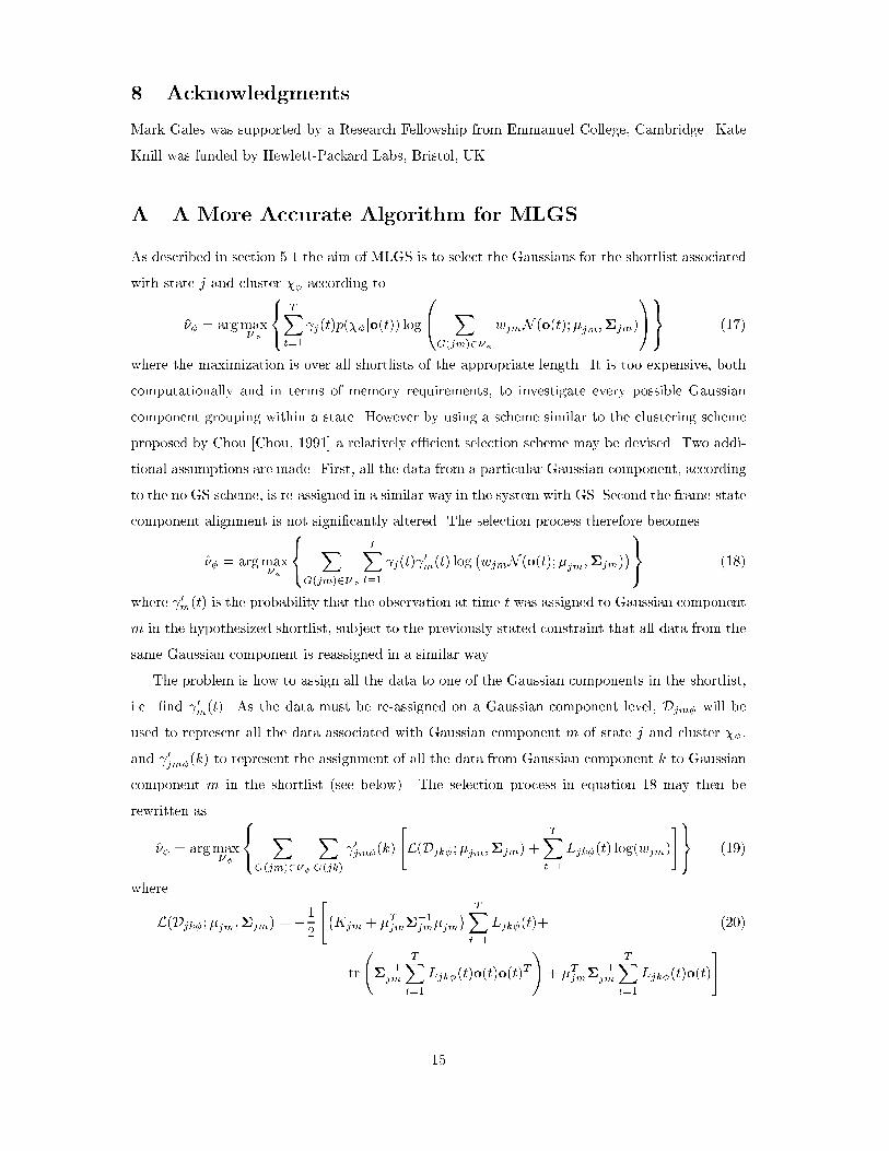
8 AcknowledgmentsMark Gales was supported by a Research Fellowship from Emmanuel College, Cambridge. KateKnill was funded by Hewlett-Packard Labs, Bristol, UK.A A More Accurate Algorithm for MLGSAs described in section 5.1 the aim of MLGS is to select the Gaussians for the shortlist associatedwith state j and cluster �� according to�̂� = argmax�� 8<: TXt=1 j(t)p(��jo(t)) log0@ XG(jm)2�� wjmN (o(t);�jm;�jm)1A9=; (17)where the maximization is over all shortlists of the appropriate length. It is too expensive, bothcomputationally and in terms of memory requirements, to investigate every possible Gaussiancomponent grouping within a state. However by using a scheme similar to the clustering schemeproposed by Chou [Chou, 1991] a relatively e�cient selection scheme may be devised. Two addi-tional assumptions are made. First, all the data from a particular Gaussian component, accordingto the no GS scheme, is re-assigned in a similar way in the system with GS. Second the frame-statecomponent alignment is not signi�cantly altered. The selection process therefore becomes�̂� = argmax�� 8<: XG(jm)2�� TXt=1 j(t) 0m(t) log �wjmN (o(t);�jm;�jm)�9=; (18)where 0m(t) is the probability that the observation at time t was assigned to Gaussian componentm in the hypothesized shortlist, subject to the previously stated constraint that all data from thesame Gaussian component is reassigned in a similar way.The problem is how to assign all the data to one of the Gaussian components in the shortlist,i.e. �nd 0m(t). As the data must be re-assigned on a Gaussian component level, Djm� will beused to represent all the data associated with Gaussian component m of state j and cluster ��,and 0jm�(k) to represent the assignment of all the data from Gaussian component k to Gaussiancomponent m in the shortlist (see below). The selection process in equation 18 may then berewritten as�̂� = argmax�� 8<: XG(jm)2�� XG(jk) 0jm�(k)"L(Djk�;�jm;�jm) + TXt=1 Ljk�(t) log(wjm)#9=; (19)whereL(Djk�;�jm;�jm) = �12 "�Kjm + �Tjm��1jm�jm� TXt=1 Ljk�(t)+ (20)tr ��1jm TXt=1 Ljk�(t)o(t)o(t)T!+ �Tjm��1jm TXt=1 Ljk�(t)o(t)#15

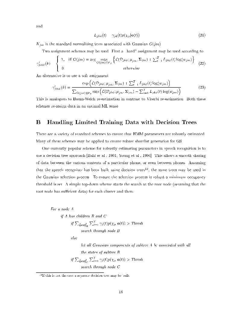
and Ljk�(t) = jk(t)p(��jo(t)) (21)Kjm is the standard normalising term associated with Gaussian G(jm).Two assignment schemes may be used. First a \hard" assignment may be used according to 0jm�(k) =8><>: 1; i� G(jm) = arg maxG(jm)2�� nL(Djk�;�jm;�jm) +PTt=1 Ljk�(t) log(wjm)o0 otherwise (22)An alternative is to use a soft assignment. 0jm�(k) = exp�L(Djk�;�jm;�jm) +PTt=1 Ljk�(t) log(wjm)�PG(jm)2�� exp�L(Djk� ;�jm;�jm) +PTt=1 Ljk�(t) log(wjm)� (23)This is analogous to Baum-Welch re-estimation in contrast to Viterbi re-estimation. Both theseschemes re-assign data in an optimal ML sense.B Handling Limited Training Data with Decision TreesThere are a variety of standard schemes to ensure that HMM parameters are robustly estimated.Many of these schemes may be applied to ensure robust shortlist generation for GS.One currently popular scheme for robustly estimating parameters in speech recognition is touse a decision tree approach [Bahl et al., 1991, Young et al., 1994]. This allows a smooth sharingof data between the various contexts of a particular phone, or even between phones. Assumingthat the speech recogniser has been built using decision trees12, the same trees may be used inthe Gaussian selection process. To ensure the selection process is robust a minimum occupancythreshold is set. A simple top-down scheme starts the search at the root node (assuming that theroot node has su�cient data) for each cluster and then:For a node Aif A has children B and Cif PLeafBPTt=1 j(t)p(��jo(t)) > Threshsearch through node Belse let all Gaussian components of subtree A be associated with allthe states of subtree Bif PLeafC PTt=1 j(t)p(��jo(t)) > Threshsearch through node C12If this is not the case a separate decision tree may be built.16

else let all Gaussian components of subtree A be associated with allthe states of subtree Celse let all Gaussian components of subtree A be associated with all thestates of subtree Awhere LeafB indicates all leaves of subtree B. Using this scheme the set of Gaussian componentsto be associated with each state is easily derived. The selection process to be used determines howthis information is to be used. For the standard MLGS scheme the following selection process isused.G(jm) 2 �� i� G(jm) 2 argmaxm (n)8<: Xk2s(j) TXt=1 k(t)p(��jo(t)) log �wjmN (o(t);�jm;�jm)�9=;(24)where s(j) is the list of all Gaussian components associated with state j as determined by thedecision tree. For the accurate MLGS scheme described in appendix A, all Gaussian componentsassociated with state j must be assigned to one of the Gaussian components in the hypothesisedshortlist, i.e. 0jm�(k) is calculated for all Gaussian components.

17

References[Bahl et al., 1991] Bahl, L. R., de Souza, P. V., Gopalkrishnan, P. S., Nahamoo, D., and Picheny,M. A. (1991). Context dependent modelling of phones in continuous speech using decision trees.In Proceedings DARPA Speech and Natural Language Processing Workshop, pages 264{270.[Beyerlein, 1994] Beyerlein, P. (1994). Fast log-likelihood computation for mixture densities in ahigh-dimensional feature space. In Proc. ICSLP, pages 271{274, Yokohama.[Beyerlein and Ullrich, 1995] Beyerlein, P. and Ullrich, M. (1995). Hamming distance approxi-mation for a fast log-likelihood computation for mixture densities. In Proc. Eurospeech, pages1083{1086, Madrid.[Bocchieri, 1993] Bocchieri, E. (1993). Vector quantization for e�cient computation of continuousdensity likelihoods. In Proc. ICASSP, volume II, pages II{692{II{695, Minneapolis.[Chou, 1991] Chou, P. (1991). Optimal partitioning for classi�cation and regression trees. IEEETrans PAMI, 13:348.[Fritsch and Rogina, 1996] Fritsch, J. and Rogina, I. (1996). The bucket box intersection (BBI)algorithm for fast approximate evaluation of diagonal mixture gaussians. In Proc. ICASSP,volume 2, pages II{273{II{276, Atlanta.[Huang et al., 1990] Huang, X. D., Lee, K. F., and Hon, H. W. (1990). On semi-continuous hiddenMarkov modelling. In Proc. ICASSP, pages 689{692.[Hunt and Lefebre, 1989] Hunt, M. and Lefebre, C. (1989). A comparison of several acousticrepresentations for speech recognition with degraded and undegraded speech. In ProceedingsICASSP, pages 262{265.[Knill et al., 1996] Knill, K. M., Gales, M. J. F., and Young, S. (1996). Use of Gaussian selectionin large vocabulary continuous speech recognition using HMMs. In Proc. ICSLP, volume 1,pages I{470{I{473, Philadelphia.[Linde et al., 1980] Linde, Y., Buzo, A., and Gray, R. M. (1980). An algorithm for vector quantizerdesign. IEEE Trans Comms, COM-28(1):84{95.[Murveit et al., 1994] Murveit, H., Monaco, P., Digalakis, V., and Butzberger, J. (1994). Tech-niques to achieve an accurate real-time large-vocabulary speech recognition system. In Proc.ARPA Workshop on Human Language Technology, pages 368{373, Plainsboro, N.J.[Odell et al., 1994] Odell, J. J., Valtchev, V., Woodland, P. C., and Young, S. J. (1994). A one passdecoder design for large vocabulary recognition. In Proceedings ARPA Workshop on HumanLanguage Technology, pages 405{410. 18

[Ortmanns et al., 1997] Ortmanns, S., Firzla�, T., and Ney, H. (1997). Fast likelihood compu-tation methods for continuous mixture densities in large vocabulary speech recognition. InProceedings Eurospeech, pages 139{142.[Pallett et al., 1995] Pallett, D. S., Fiscus, J. G., Fisher, W. M., Garofolo, J. S., Lund, B. A.,Martin, A., and Przybocki, M. A. (1995). 1994 benchmark tests for the ARPA spoken languageprogram. In Proceedings ARPA Workshop on Spoken Language Systems Technology, pages 5{36.[Poggi, 1993] Poggi, G. (1993). Fast algorithm for full-search VQ encoding. Electronics Letters,29(12):1141{1142.[Woodland et al., 1995] Woodland, P. C., Odell, J. J., Valtchev, V., and Young, S. J. (1995).The development of the 1994 HTK large vocabulary speech recognition system. In ProceedingsARPA Workshop on Spoken Language Systems Technology, pages 104{109.[Young et al., 1994] Young, S. J., Odell, J. J., and Woodland, P. C. (1994). Tree-based state tyingfor high accuracy acoustic modelling. In Proceedings ARPA Workshop on Human LanguageTechnology, pages 307{312.

19

C BiographiesMark J.F. Gales studied for the B.A. in Electrical and Information Sciences at the Universityof Cambridge from 1985-88. Following graduation he worked as a consultant at Roke ManorResearch Ltd. In 1991 he took up a position as a Research Associate in the Speech Vision andRobotics group if the Engineering Department at Cambridge University. In 1996 he completed hisdoctoral thesis: Model-Based Techniques for Robust Speech Recognition. From 1995-1997 he wasa Research Fellow at Emmanuel College Cambridge. He is currently a Research Sta� Member inthe Speech goup at the IBM T.J.Watson Research Center. His research interests include robustspeech recognition, speaker adaptation, segmental models of speech and large-vocabulary speechrecognition.Katherine M. Knill (S'90, M'94) received the BEng Degree in electronic engineering andmathematics from Nottingham University, England, in 1990, and the PhD and DIC degrees fromImperial College, London University, England, in 1994. She was sponsored during this time (1986-1993) by Marconi Underwater Systems Ltd, England. In October 1993 she joined the Speech,Vision and Robotics Group at Cambridge University, England. Her primary research focus waskeyword spotting for audio document retrieval, in collaboration with Hewlett-Packard Labs, Bris-tol, England. She is currently working for Nuance Communications, Menlo Park, CA, which shejoined in January 1997. A member of the algorithms group, she works on developing commercialtelephone-based automatic speech recognition system.Stephen J. Young completed the PhD in speech synthesis in 1977 after taking a First inelectrical sciences, both at Cambridge University, UK. He took a Lectureship at UMIST beforejoining the Cambridge University Engineering Department in 1984 as a Lecturer and Fellow ofEmmanuel College. He was promoted to a Readership in October 1994 and elected to the Chairof Information Engineering in December 1994. His research intersets include speech recognition,language modelling and multimedia applications. He is currently head of the Speech, Vision andRobotics (SVR) Group and he is Technical Director of Entropic Cambridge Research Ltd . He isa Fellow of the Institute of Acoustics and European Editor of Computer Speech and Language.

20

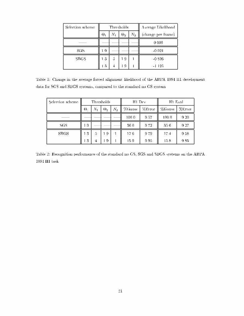
Selection scheme Thresholds Average Likelihood�1 N1 �2 N2 (change per frame)| | | | | 0.000SGS 1.9 | | | -0.021SBGS 1.3 5 1.9 1 -0.8261.3 4 1.9 1 -1.125Table 1: Change in the average forced alignment likelihood of the ARPA 1994 H1 developmentdata for SGS and SBGS systems, compared to the standard no GS system.Selection scheme Thresholds H1 Dev H1 Eval�1 N1 �2 N2 %Gauss %Error %Gauss %Error| | | | | 100.0 9.57 100.0 9.20SGS 1.9 | | | 36.0 9.72 35.6 9.27SBGS 1.3 5 1.9 1 17.6 9.79 17.4 9.581.3 4 1.9 1 15.9 9.95 15.8 9.85Table 2: Recognition performance of the standard no GS, SGS and SBGS systems on the ARPA1994 H1 task.

21

Codewords Thresh. %States Assign.� ld li �(d) �(i) �(�)10.0 50.0 11.9 45.0 43.1512 20.0 50.0 8.2 48.4 43.450.0 50.0 4.6 51.9 43.5Table 3: The percentage of states assigned at each context level in MLGS and OGS. �(d) is thecontext dependent level, �(i) is the context independent level and �(�) is cluster level, with � = 1:9.Selection scheme Max. Cmpts. Average LikelihoodN1 N2 N3 (change per frame)12 2 1 -0.241MLGS (ld = 10) 6 2 1 -0.6214 2 1 -1.048MLGS (ld = 20) 6 2 1 -0.6606 1 1 -0.785MLGS (ld = 50) 6 2 1 -0.746OGS (ld = 20) 6 2 1 -0.555Table 4: Change in the average forced alignment likelihood of the ARPA 1994 H1 developmentdata for MLGS and OGS with li = 50, compared to the standard no GS system.Selection scheme Thresh. H1 Dev H1 Evalld li %Gauss %Error %Gauss %Error10.0 50.0 15.4 9.78 15.2 9.35MLGS (N2 = 2) 20.0 50.0 14.1 9.84 13.9 9.4650.0 50.0 12.6 10.11 12.5 9.41MLGS (N2 = 1) 20.0 50.0 11.4 10.02 11.2 9.49OGS (N2 = 2) 20.0 50.0 14.1 9.78 13.9 9.56Table 5: Recognition performance of MLGS and OGS on the ARPA 1994 H1 task with N1 = 6,N3 = 1 and � = 1:9. 22

Selection scheme H1 Dev H1 Eval%Gauss %Error %Gauss %Error| 100.0 9.57 100.0 9.20SGS 36.0 9.72 35.6 9.27SBGS 17.6 9.79 17.4 9.58MLGS 14.1 9.84 13.9 9.46OGS 14.1 9.78 13.9 9.56Table 6: Summary of comparative performance for the various selection schemes on the ARPA1994 H1 Task.

23