SCALABLE GAUSSIAN PROCESS METHODS FOR SINGLE ...
174
SCALABLE GAUSSIAN PROCESS METHODS FOR SINGLE-CELL DATA A thesis submitted to the University of Manchester for the degree of Doctor of Philosophy in the Faculty of Biology, Medicine and Health 2019 Sumon Ahmed School of Health Sciences
-
Upload
khangminh22 -
Category
Documents
-
view
1 -
download
0
Transcript of SCALABLE GAUSSIAN PROCESS METHODS FOR SINGLE ...

SCALABLE GAUSSIAN PROCESS
METHODS FOR SINGLE-CELL DATA
A thesis submitted to the University of Manchester
for the degree of Doctor of Philosophy
in the Faculty of Biology, Medicine and Health
2019
Sumon Ahmed
School of Health Sciences

Contents
Abstract 11
Declaration 12
Copyright 13
Acknowledgements 14
1 Introduction 16
1.1 Motivation . . . . . . . . . . . . . . . . . . . . . . . . . . . . . . . 18
1.2 Aims and objectives . . . . . . . . . . . . . . . . . . . . . . . . . 20
1.3 Thesis outline . . . . . . . . . . . . . . . . . . . . . . . . . . . . . 21
2 Background 23
2.1 Pseudotime and trajectory inference . . . . . . . . . . . . . . . . . 24
2.1.1 Pseudotime and trajectory inference algorithms . . . . . . 24
2.1.2 Differential expression and branching . . . . . . . . . . . . 33
2.2 Gaussian process inference . . . . . . . . . . . . . . . . . . . . . . 35
2.2.1 Covariance function . . . . . . . . . . . . . . . . . . . . . . 36
2.2.2 GP regression . . . . . . . . . . . . . . . . . . . . . . . . . 42
2.2.3 Sparse GP regression . . . . . . . . . . . . . . . . . . . . . 44
2.2.4 Gaussian process latent variable model . . . . . . . . . . . 47
2.2.5 Overlapping mixture of Gaussian processes . . . . . . . . . 48
2.2.6 Gaussian process software packages . . . . . . . . . . . . . 48
2.3 Gaussian process methods for single-cell data . . . . . . . . . . . . 49
2.3.1 Pseudotime inference . . . . . . . . . . . . . . . . . . . . . 49
2.3.2 Differential expression and branching . . . . . . . . . . . . 51
2

3 Probabilistic pseudotime estimation 54
3.1 GrandPrix: Scaling up the Bayesian GPLVM . . . . . . . . . . . . 54
3.1.1 Model . . . . . . . . . . . . . . . . . . . . . . . . . . . . . 55
3.1.2 Inference . . . . . . . . . . . . . . . . . . . . . . . . . . . . 56
3.2 Results and discussion . . . . . . . . . . . . . . . . . . . . . . . . 59
3.2.1 Inferring withheld time points and smooth pseudotime tra-
jectories . . . . . . . . . . . . . . . . . . . . . . . . . . . . 60
3.2.2 Correctly identifying precocious cells . . . . . . . . . . . . 63
3.2.3 Recovering cell cycle peak times . . . . . . . . . . . . . . . 66
3.2.4 Recovering Diffusion Pseudotime (DPT) . . . . . . . . . . 68
3.2.5 2D visualization of ∼68k Peripheral Blood Mononuclear
Cells (PBMCs) . . . . . . . . . . . . . . . . . . . . . . . . 70
3.2.6 Extending the model to infer pseudotime-branching . . . . 77
3.3 Summary . . . . . . . . . . . . . . . . . . . . . . . . . . . . . . . 87
4 Uncovering gene-specific branching 90
4.1 DEtime model . . . . . . . . . . . . . . . . . . . . . . . . . . . . . 90
4.1.1 Extension to non-Gaussian likelihood . . . . . . . . . . . . 94
4.1.2 Inference . . . . . . . . . . . . . . . . . . . . . . . . . . . . 95
4.2 Identifying differentially expressed genes using single-cell data . . 98
4.3 Branching Gaussian Process (BGP) . . . . . . . . . . . . . . . . . 111
4.3.1 Branching kernel . . . . . . . . . . . . . . . . . . . . . . . 112
4.3.2 Inference . . . . . . . . . . . . . . . . . . . . . . . . . . . . 113
4.3.3 BGP results . . . . . . . . . . . . . . . . . . . . . . . . . . 116
4.3.4 Limitations of the BGP . . . . . . . . . . . . . . . . . . . 117
4.4 Multivariate BGP (mBGP) . . . . . . . . . . . . . . . . . . . . . 122
4.4.1 Inference . . . . . . . . . . . . . . . . . . . . . . . . . . . . 123
4.4.2 Experimental results . . . . . . . . . . . . . . . . . . . . . 126
4.5 Summary . . . . . . . . . . . . . . . . . . . . . . . . . . . . . . . 132
5 Conclusion 134
5.1 Accomplished results . . . . . . . . . . . . . . . . . . . . . . . . . 135
5.2 Research output . . . . . . . . . . . . . . . . . . . . . . . . . . . . 138
5.3 Future work . . . . . . . . . . . . . . . . . . . . . . . . . . . . . . 139
5.3.1 Pseudotime inference . . . . . . . . . . . . . . . . . . . . . 139
5.3.2 Branching inference . . . . . . . . . . . . . . . . . . . . . . 140
3

5.3.3 Inferring pseudotime-branching . . . . . . . . . . . . . . . 141
A Additional material for Chapter 3 158
A.1 Sparse GP Regression . . . . . . . . . . . . . . . . . . . . . . . . 158
A.2 Sparse GPLVM . . . . . . . . . . . . . . . . . . . . . . . . . . . . 162
A.3 Roughness statistics . . . . . . . . . . . . . . . . . . . . . . . . . 166
B Additional material for Chapter 4 167
B.1 Derivation of multivariate branching Gaussian process (mBGP) . 167
B.1.1 Sparse approximation . . . . . . . . . . . . . . . . . . . . . 173
Word Count: 34547
4

List of Tables
2.1 An overview of some popular pseudotime and trajectory inference
methods. . . . . . . . . . . . . . . . . . . . . . . . . . . . . . . . . 53
3.1 Number of iterations to convergence required by GrandPrix ini-
tialised using tSNE to optimise 2D latent spaces from∼68k PBMCs
for different number of inducing points. . . . . . . . . . . . . . . . 76
3.2 Fitting time required per iteration by GrandPrix initialised using
tSNE to optimise 2D latent spaces from ∼68k PBMCs for different
number of inducing points. . . . . . . . . . . . . . . . . . . . . . . 77
4.1 Posterior cell assignment to the top branch by BGP for the top six
biomarkers of hematopoietic stem cells (HSCs) . . . . . . . . . . . 120
4.2 Percentage (%) of cell assignment consistency achieved by BGP
for each pair of the top six biomarkers of hematopoietic stem cells
(HSCs) . . . . . . . . . . . . . . . . . . . . . . . . . . . . . . . . . 122
4.3 Comparison of prior and posterior cell assignment for the mBGP
model . . . . . . . . . . . . . . . . . . . . . . . . . . . . . . . . . 132
5

List of Figures
2.1 Illustration of the squared exponential covariance function . . . . 37
2.2 Illustration of the OU-process covariance function . . . . . . . . . 39
2.3 Samples from the Matern3/2 and Matern5/2 covariance functions. . 39
2.4 Illustration of the smooth periodic covariance function . . . . . . 40
2.5 Illustration of the quasi-periodic OU-process covariance function . 41
2.6 Gaussian process regression . . . . . . . . . . . . . . . . . . . . . 44
3.1 Comparison between actual cell capture times and estimated pseu-
dotimes using GPLVM for Arabidopsis thaliana microarray data . 61
3.2 Comparison of performance and fitting time between GrandPrix
and DeLorean for Arabidopsis thaliana microarray data . . . . . . 62
3.3 Average roughness statistics of estimated pseudotime using Grand-
Prix for Arabidopsis thaliana data. . . . . . . . . . . . . . . . . . 64
3.4 Estimated pseudotime for mouse dendritic cells using GrandPrix
and comparison of fitting time required by both DeLorean and
GrandPrix for different number of inducing points . . . . . . . . . 65
3.5 Expression profiles over estimated pseudotime for some selected
genes from PC3 human prostate cancer cell line . . . . . . . . . . 67
3.6 Comparison of GrandPrix estimated pseudotime for mouse embry-
onic stem cells with the actual cell capture time and the pseudotime
estimated using DPT . . . . . . . . . . . . . . . . . . . . . . . . . 69
3.7 Comparison of GrandPrix estimated pseudotime without using in-
formative prior for mouse embryonic stem cells with the actual cell
capture time and the pseudotime estimated using DPT . . . . . . 71
3.8 Time required by GrandPrix per iteration for ∼68k peripheral
blood mononuclear cells (PBMCs) when using different number
of CPU cores for both 32 and 64 bit floating point precision . . . 73
3.9 2D visualisation of∼68k peripheral blood mononuclear cells (PBMCs) 75
6

3.10 Comparison of the adjusted rand index (ARI) values of the models
with different initialisations and experimental setups . . . . . . . 76
3.11 Lower dimensional representations of the single-cell qPCR data
from early developmental stages using PCA and the Bayesian GPLVM
with prior mean in one latent dimension based on capture times . 78
3.12 Latent space reconstruction using the Bayesian GPLVM without
and with prior for the single-cell qPCR data from early develop-
mental stages . . . . . . . . . . . . . . . . . . . . . . . . . . . . . 80
3.13 Comparison between the actual capture times and the GrandPrix
estimated pseudotimes from the 2-D and 1-D model with infor-
mative prior for single-cell qPCR data from early developmental
stages . . . . . . . . . . . . . . . . . . . . . . . . . . . . . . . . . 81
3.14 The expression profiles of the two known markers genes against
the estimated pseudotime from single-cell qPCR data of early de-
velopmental stages . . . . . . . . . . . . . . . . . . . . . . . . . . 82
3.15 The expression profiles of top 10 differentially expressed genes be-
tween the stages trophectoderm (TE) and epiblast (EPI) against
the estimated pseudotime for single-cell qPCR data of early devel-
opmental stages . . . . . . . . . . . . . . . . . . . . . . . . . . . . 83
3.16 The expression profiles of top 10 differentially expressed genes
between the stages primitive endoderm (PE) and epiblast (EPI)
against the estimated pseudotime for single-cell qPCR data of early
developmental stages . . . . . . . . . . . . . . . . . . . . . . . . . 84
3.17 The expression profiles of top 10 differentially expressed genes
between the stages trophectoderm (TE) and primitive endoderm
(PE) against the estimated pseudotime for single-cell qPCR data
of early developmental stages . . . . . . . . . . . . . . . . . . . . 85
3.18 Heatmap showing the expression profiles of 48 genes from single-
cell qPCR data of early developmental stages across the estimated
pseudotime as well as the added extra latent dimension . . . . . . 86
3.19 Effect of changing the prior variance on the estimated pseudotime
for single-cell qPCR data of early developmental stages . . . . . . 88
4.1 Illustration of branching kernel for two latent functions . . . . . . 93
4.2 Examples of the DEtime model fit on Arabidopsis thaliana time
series for a gene with perturbation and a gene without perturbation 99
7

4.3 Examples of the DEtime model fit on Arabidopsis thaliana time
series for an early and a late perturbation genes . . . . . . . . . . 100
4.4 DEtime with Gaussian likelihood model fit on the mouse haematopoi-
etic stem cells (HSCs) for an early and a late branching genes . . 102
4.5 DEtime with negative binomial (NB) likelihood model fit on the
mouse haematopoietic stem cells (HSCs) for an early and a late
branching genes . . . . . . . . . . . . . . . . . . . . . . . . . . . . 104
4.6 DEtime with Gaussian likelihood model fit on the top six biomark-
ers of mouse haematopoietic stem cells (HSCs) . . . . . . . . . . . 105
4.7 DEtime with negative binomial (NB) likelihood model fit on the
top six biomarkers of mouse haematopoietic stem cells (HSCs) . . 106
4.8 DEtime model fit on the expression profile of marker IRF8 from
mouse haematopoietic stem cells (HSCs) . . . . . . . . . . . . . . 108
4.9 DEtime model fit on the expression profile of marker APOE from
mouse haematopoietic stem cells (HSCs) . . . . . . . . . . . . . . 109
4.10 DEtime model fit on the expression profile of marker ERP29 from
mouse haematopoietic stem cells (HSCs) . . . . . . . . . . . . . . 110
4.11 Illustration of branching kernel for 3 latent functions . . . . . . . 114
4.12 Branching GP (BGP) fit for the early branching gene MPO from
mouse haematopoietic stem cells (HSCs) . . . . . . . . . . . . . . 118
4.13 Example of inconsistent cell assignments by Branching GP (BGP)
while using a strong prior assignment probability of 0.80 . . . . . 121
4.14 Example of inconsistent cell assignments by Branching GP (BGP)
while using a very strong prior assignment probability of 0.99 . . . 121
4.15 Multivariate branching GP (mBGP) model fit on a simulated dataset127
4.16 Multivariate branching GP (mBGP) model fit on genes showing
very strong evidence of branching from mouse haematopoietic stem
cells (HSCs) . . . . . . . . . . . . . . . . . . . . . . . . . . . . . . 130
4.17 Multivariate branching GP (mBGP) model fit on the expression
profile of 12 genes having strong evidence of branching from mouse
haematopoietic stem cells (HSCs) . . . . . . . . . . . . . . . . . . 131
8

List of Abbreviations
AGA Approximate graph abstraction
ARI Adjusted rand index
BEAM Branch expression analysis modelling
BGP Branching Gaussian process
DE Differentially expressed
DPT Diffusion pseudotime
EPI Epiblast
FDR False discovery rate
FITC Fully Independent Training Conditional
GLM Generalized linear modeling
GP Gaussian process
GPLVM Gaussian process latent variable model
HCA Human Cell Atlas
hESC Human embryonic stem cell
HMC Hamiltonian Monte Carlo
HMM Hidden Markov model
HSC Hematopoietic stem cell
HSMM Human skeletal muscle myoblasts
ICA Independent components analysis
KNN K-nearest-neighbour
LHS Latin Hypercube Sampling
mBGP Multivariate branching Gaussian process
MCMC Markov Chain Monte Carlo
MS Mean square
ML Machine learning
MST Minimum spannig tree
9

OMGP Overlapping Mixture of Gaussian Processes
OU Ornstein-Uhlenbeck
PBMC Peripheral blood mononuclear cell
PCA Principal components analysis
PE Primitive endoderm
PMF Probability mass function
qNSC Quiescent neural stem cells
RBF Radial basis function
RMSE Root mean square error
RNA-seq RNA-sequencing
sc Single-cell
SCDS Single-cell data science
SE Squared exponential
TE Trophectoderm
TI Trajectory inference
tSNE t-Stochastic neighbourhood embedding
UMAP Uniform manifold approximation and projection
VFE Variational Free Energy
VI Variational inference
10

The University of Manchester
Sumon AhmedFaculty of Biology, Medicine and HealthSchool of Health SciencesDivision of Informatics, Imaging and Data SciencesDoctor of PhilosophyScalable Gaussian process methods for single-cell dataJanuary 11, 2020
The analysis of single-cell data creates the opportunity to examine the tempo-ral dynamics of complex biological processes where the generation of time courseexperiments is challenging or technically impossible. One popular approach is tolearn a lower dimensional manifold or trajectory through the data that capturesmajor sources of variation in the data. Gene expression patterns can then bealigned through different lineages in the trajectory as smooth functions of pseu-dotime which promises to facilitate the identification of differentially expressed(DE) genes across trajectories.
We briefly review some popular trajectory inference and downstream anal-ysis methods along with their strengths and assumptions. We provide a briefoverview of Gaussian process (GP) inference and describe how GPs can be usedfor dimensionality reduction and data association, which later facilitate proba-bilistic pseudotime estimation and downstream analysis to inferring DE genesand branching times.
We present a scalable implementation of the Gaussian process latent vari-able model (GPLVM) and develop a pseudotime estimation method that scalesto droplet-based large volume single-cell datasets and can be extended to higherdimensional latent spaces to capture other sources of variation such as branch-ing dynamics. The model’s efficacy is evaluated on a number of datasets fromdifferent organisms collected using different protocols. The model converges sig-nificantly faster compared to existing methods whilst achieving comparable esti-mation accuracy.
We reimplement an existing downstream analysis method for identifying branch-ing dynamics from bulk time series data and apply it on single-cell data after pseu-dotime inference, extending the models to model counts data. We also present thelimitations of a recent approach to inference of branching dynamics in single-celldata and extend the model to mitigate its limitations. Our downstream analysismodels are shown to successfully identify branching locations for individual geneswhen applied on simulated data and single-cell mouse haematopoietic stem cells(HSCs) data.
11

Declaration
No portion of the work referred to in this thesis has been
submitted in support of an application for another degree
or qualification of this or any other university or other
institute of learning.
12

Copyright
i. The author of this thesis (including any appendices and/or schedules to
this thesis) owns certain copyright or related rights in it (the “Copyright”)
and s/he has given The University of Manchester certain rights to use such
Copyright, including for administrative purposes.
ii. Copies of this thesis, either in full or in extracts and whether in hard or
electronic copy, may be made only in accordance with the Copyright, De-
signs and Patents Act 1988 (as amended) and regulations issued under it
or, where appropriate, in accordance with licensing agreements which the
University has from time to time. This page must form part of any such
copies made.
iii. The ownership of certain Copyright, patents, designs, trademarks and other
intellectual property (the “Intellectual Property”) and any reproductions of
copyright works in the thesis, for example graphs and tables (“Reproduc-
tions”), which may be described in this thesis, may not be owned by the
author and may be owned by third parties. Such Intellectual Property and
Reproductions cannot and must not be made available for use without the
prior written permission of the owner(s) of the relevant Intellectual Property
and/or Reproductions.
iv. Further information on the conditions under which disclosure, publication
and commercialisation of this thesis, the Copyright and any Intellectual
Property and/or Reproductions described in it may take place is available
in the University IP Policy (see http://documents.manchester.ac.uk/
DocuInfo.aspx?DocID=24420), in any relevant Thesis restriction declara-
tions deposited in the University Library, The University Library’s regula-
tions (see http://www.library.manchester.ac.uk/about/regulations/)
and in The University’s policy on presentation of Theses.
13

Acknowledgements
First and foremost, I would like to thank my supervisor Professor Magnus Rattray
whose excellent support and mentorship turned my PhD studies into quite a
memorable and exhilarating adventure. It is his continuous effort in showing
me the right path towards my ultimate goal that has brought me near the final
destination of my three-year journey. Magnus shared a lot of his ideas with
me and encouraged me to explore them in my own ways which enhanced my
critical thinking capacity, and ultimately contributed towards building up my
research skills. His mentorship was not just limited within the boundaries of
academia; he motivated me to be a better human being: someone who is more
patient, composed, sympathetic and humble. It has been a privilege to have
the opportunity to work with him, to know him and I am looking forward to
collaborating with him in the following years.
Secondly, I would like to thank my co-supervisor Alexis Boukouvalas for his in-
valuable guidance during the first half of my PhD for providing me with hands-on
training on probabilistic modelling, especially on Gaussian process, and helping
me boost up my confidence. Alexis was always there to explain everything to
me point by point and with utmost care. No matter what difficulty I was going
through, he was constantly there to help me out.
I would like to thank Nuha for collaborating the work presented in Chapter 4.
Thank you Joanne, and Peyman for helping me in the proofreading process and
providing valuable insights in better elaborating the arguments in the thesis. A
special thanks to Joanne for spending a considerate amount of time till the very
last moment.
I would also like to thank Syed to familiarise me with single-cell technology.
Thanks for being the ready stock for my favourite snack items; without them, I
would not have been able to work long hours at the office. I express my gratitude
to Jing, Lijing and Mudassar for their warm and welcoming attitude; they were
14

always there by my side since the very first day. I would also like to acknowledge
Jamie, Robert and Rebecca for their constant support.
I specially express my gratitude to the Commonwealth Scholarship Commis-
sion (CSC) for funding my studies. My thanks go to the University of Manchester
that provided me with all the necessary facilities one could ask for in making
one’s PhD studies a smooth and pleasing one. I will always cherish the memories
I made at UoM, at the corridors of Smith Building, and on the pavements of
Oxford Road.
Beyond the academic grounds, I would like to acknowledge my friends who
created a second home away from home for me. Thanks to Shaown and Mahbub
for all those late night hangouts and gossips. Thanks to all my friends based in
Manchester for the fun times we have had together, especially for all the energetic
and challenging badminton sessions; these sessions could really help me escape
from the stress of research. I feel myself lucky to be part of this great community
for the last three years.
Back home, I would like to thank my wife Daisy for her endless patience and
always keeping faith in me. This thesis would never be a reality without her
endless support, inspiration, and motivation from the other end of the globe. I
want to thank her for being a crucial part of my journey. Thank you for being
the light during the times of darkness when I got completely lost about what to
do next, for believing in my abilities no matter what.
Finally, I express my gratitude to my parents to whom I am forever indebted
to for all my achievements, for whatever I am today. I am sure they would have
been the happiest to see me grow and achieve whatever I have achieved today. I
dedicate this thesis to them.
15

Chapter 1
Introduction
In recent years, the field of functional genomics has advanced very rapidly and the
analysis of single-cell data is now playing a very important role. The assaying
of the single-cell transcriptome has gained widespread popularity over the last
few years. The first single-cell RNA-sequencing (RNA-seq) study was introduced
ten years back by Tang et al. (2009), where a single 4-cell mouse blastomere was
isolated manually. The RNA sequencing procedure was carried out for each cell
individually. The motivation of the study was to produce embryonic samples cap-
turing the richness of gene expression profiles compared to microarray techniques.
Since this first study, there has been continuously growing interests in assaying
single-cells at higher resolution and on a larger scale.
In 2012, Ramskold et al. (2012) developed a robust single-cell sequencing
protocol Smart-Seq that could give full length read coverage across transcripts.
Smart-Seq was based on the SMART template switching technology and the
sequencing data produced was more familiar to the users of traditional RNA-
seq. Thus bioinformatics analysis techniques, specially at the pre-processing stage
were easily applicable on this data (Hwang et al., 2018). For example, to align the
reads form single-cell RNA-seq experiments, the same Burrows-Wheeler Aligner
(BWA) (Li and Durbin, 2010) or STAR (Dobin et al., 2013) aligner can be used.
However, for downstream analysis specialised tools and algorithms are to be used
for single cell RNA-seq data due to the difference in the nature of single cell
RNA-seq data. For instance, Vallejos et al. (2017) have shown how three bulk
RNA-seq normalisation methods, i.e. reads per million (RPM), DESeq (Anders
and Huber, 2010) and trimmed mean of M values (TMM) (Robinson and Oshlack,
2010) that are commonly used for normalising single-cell RNA-seq can produce
16
CHAPTER 1. INTRODUCTION 17
misleading results. They have also examined two methods BASiCS (Vallejos
et al., 2015) and scran (Lun et al., 2016) developed for single-cell data analysis
and have highlighted the importance of using single-cell analysis pipelines instead
of bulk analysis pipelines to take the full advantages of the richness of single-cell
data. More recently, Laehnemann et al. (2019) have described the data science
challenges which are unique to single-cell data and have given rise to the era of
Single-Cell Data Science (SCDS). The authors have highlighted twelve central
grand challenges of SCDS as well as the current status and future opportunities
of this emerging new research area.
Later the Smart-Seq protocol was refined to develop Smart-Seq2 that signifi-
cantly reduced the library preparation cost and helped single-cell RNA-sequencing
gain attention on a global scale (Picelli et al., 2013, 2014). In the following years,
single-cell protocols continued to improve very rapidly and nowadays it is possible
to assay tens of thousands of cells by using droplet based techniques such as Drop-
seq (Macosko et al., 2015) as well as the massively parallel 10x platform (Zheng
et al., 2017).
This mass production of single-cell data has opened the doors to examining
complex biological systems more closely, ranging from the microbial ecosystem to
the genomics of human cancer (Gawad et al., 2016). In single-cell technology the
transcriptome of each cell is measured individually, in contrast to the bulk RNA-
seq technology where the measurement is performed by averaging gene expression
across a cell population. Averaging transcriptomes across a cell population fails
to capture transcriptomic variation across individual cells. Recent studies have
shown that many questions can be answered in a more refined way at single-
cell level (see e.g. Gawad et al., 2016; Hwang et al., 2018). For instance, during
differentiation, each cell defines its fate based on the signal received from other
cells and other stimuli. Moreover, the developmental rate is not the same in
each cell across a cell population, hence similar changes in transcriptomes can
be observed at varying time scales for different cells. Therefore, averaging the
expression profiles across a population of cells in a bulk analysis fails to mimic
the true picture of the developmental and differential processes at the cellular
level.
Examining the differences in gene expression at single-cell level can facilitate
the identification of novel cell types which is not possible by analysing bulk gene
expression. Single-cell data have been used to identify multiple distinct as well

CHAPTER 1. INTRODUCTION 18
as rare cell types (Grun et al., 2015; Kolodziejczyk et al., 2015). Single-cell data
have been used to detect outliers within a cell population that promises to help
researchers understand drug resistance and relapse in cancer treatment (Shaf-
fer et al., 2017). Single-cell RNA-seq have also been used to identify different
subtypes of neuron cells (see Poulin et al. (2016) for a review). The ambitious
Human Cell Atlas (HCA) project aims to construct a comprehensive map of the
human body similar to google map for cities (Regev et al., 2017). The project
aims to characterise all cells in a healthy human body, their numbers, locations,
types and molecular compositions. Once completed, it is expected to provide a
3D map of how cells work together to make tissues and how changes in this map
is altered between healthy and diseased cells.
Single-cell sequencing has been used extensively to study differentiating cells,
tracking changes in gene expression as cells progress. Early examples include
identifying switch-like changes in gene expression profiles by reconstructing the
trajectory of differentiating primary human myoblasts (Trapnell et al., 2014),
as well as the identification of bi-potent progenitor cells by analysing the lin-
eage structure of differentiating alveolar cells from mouse (Treutlein et al., 2014).
Single-cell sequencing has been used to study differentiating hematopoietic stem
cells (HSCs) (Paul et al., 2015; Kowalczyk et al., 2015; Zhou et al., 2016), differ-
entiating CD4+ T cells (Lonnberg et al., 2017; Stubbington et al., 2016) and more
recently Cao et al. (2019) provide a global view of mammalian organ development
by using single-cell data from mice.
1.1 Motivation
While the analysis of single-cell genomics data promises to reveal novel states of
complex biological processes, it is challenging due to inherent biological and tech-
nical noise. It is often useful to reduce high-dimensional single-cell gene expression
profiles into a low-dimensional latent space capturing major sources of inter-cell
variation in the data. Popular methods for dimensionality reduction applied to
single-cell data include linear methods such as Principal and Independent Com-
ponents Analysis (P/ICA) (Trapnell et al., 2014; Ji and Ji, 2016) and non-linear
techniques such as t-stochastic neighbourhood embedding (tSNE) (Maaten and
Hinton, 2008; Becher et al., 2014), diffusion maps (Haghverdi et al., 2015, 2016),
Uniform manifold approximation and projection (UMAP) (McInnes et al., 2018;

CHAPTER 1. INTRODUCTION 19
Cao et al., 2019) and the Gaussian Process Latent Variable Model (GPLVM) (Lawrence,
2005; Buettner and Theis, 2012; Buettner et al., 2015). In some cases the dimen-
sion is reduced to a single pseudotime dimension representing the trajectory of
cells undergoing some dynamic process such as differentiation or cell division. The
trajectory may be linear, branching or even cyclic depending on the underlying
process.
Different formalisms are used to represent a pseudotime trajectory. In graph-
based methods (Trapnell et al., 2014; Bendall et al., 2014; Shin et al., 2015;
Ji and Ji, 2016), a simplified graph or tree is estimated. By using different
path-finding algorithms, these methods try to find a path through a series of
nodes. These nodes can correspond to individual cells (Trapnell et al., 2014;
Bendall et al., 2014) or groups of cells (Shin et al., 2015; Ji and Ji, 2016) in the
graph. Another group of methods (Marco et al., 2014; Campbell et al., 2015;
Street et al., 2018) uses curve fitting to characterize the pseudotime trajectory.
Principal curves are used to model the trajectory and each cell is assigned a
pseudotime according to its low-dimensional projection on the principal curves.
On the other hand, in the diffusion pseudotime (DPT) framework (Haghverdi
et al., 2016), there is no initial dimension reduction. DPT uses random walk
based inference where all the diffusion components are used to infer pseudotime.
There are also probabilistic approaches that infer pseudotemporal ordering of cells
within the Bayesian framework considering associated uncertainty in pseudotime
estimation (Campbell and Yau, 2016; Reid and Wernisch, 2016; Strauß et al.,
2018).
The downstream analysis of trajectory inference needs to track changes in gene
expression profiles during dynamic processes such as cell cycle, cellular activation
or cell type differentiation. To understand the underlying biological process, it
is important to identify genes that are differentially expressed across multiple
lineages in the trajectory. Moreover, it is also interesting to discover gene-specific
branching locations, i.e. to identify genes following the global branching structure
as well as genes that start differentiating early or late compared to the cellular
branching point. Currently there are few such methods. The tradeSeq pack-
age (Van den Berge et al., 2019) provides a number of statistical tests to identify
DE genes, while BEAM (Qiu et al., 2017a) and GPfates (Lonnberg et al., 2017)
provide additional functionality for estimating branching locations of individual

CHAPTER 1. INTRODUCTION 20
genes. Boukouvalas et al. (2018) have developed a probabilistic approach to iden-
tifying gene-specific branching times that considers the associated uncertainty in
assigning cells to different lineages, and that approach is further developed in this
thesis.
Gene expression can be extremely noisy at the single-cell level, which demands
the development of probabilistic approaches for both trajectory inference as well
as downstream analysis. Single-cell datasets are becoming available in larger
volumes day by day, for example, Cao et al. (2019) recently assayed approximately
2 million cells. Therefore it is vital that single-cell analysis tools are scalable to
increasing number of cells. While there are probabilistic methods for analysing
single-cell data, they are often not computationally efficient enough to work with
larger datasets. Therefore, there is a growing need for developing computationally
efficient probabilistic approaches that will scale to continuously growing single-cell
datasets.
1.2 Aims and objectives
The aim is to develop scalable models that can handle both biological and tech-
nical noise inherent in single-cell data. The approach pursued here is to develop
variational Bayesian methods, which offer a principled yet pragmatic answer to
these challenges. The core of our models is the Gaussian process which has been
used extensively to model uncertainty in regression, classification and dimension
reduction tasks (see e.g. Challis et al., 2015; Buckingham-Jeffery et al., 2018; Eyre
et al., 2018; Poolman et al., 2019; Lonnberg et al., 2017). The models we develop
are based on sparse variational approximations which require only a small num-
ber of inducing points, hence very limited computational resources to efficiently
produce a full posterior distribution.
The objectives of this project can be summarised by the following points:
• Develop a probabilistic pseudotime estimation algorithm using the varia-
tional sparse approximation of the Bayesian GPLVM (Titsias and Lawrence,
2010) allowing the incorporation of prior knowledge in the form of an in-
formative prior.
• Investigate how extending the pseudotime model to include additional la-
tent dimensions allows for improved pseudotime estimation in the case of

CHAPTER 1. INTRODUCTION 21
branching dynamics.
• Extend methods that were originally developed to identify differentially ex-
pressed (DE) genes in bulk datasets to be used in single-cell analysis to
identify DE genes along different lineages or branches in the trajectory,
comparing this approach with other single-cell downstream analysis meth-
ods.
• Develop an improved downstream analysis method to identify gene-specific
branching locations for all the genes together, unlike the existing methods
where inference is carried out for one gene at a time.
• Provide scalable and efficient implementations of our models within a flex-
ible architecture that allows numeric computations to be performed across
a number of CPU cores as well as GPUs.
1.3 Thesis outline
The main contribution of this thesis is to develop scalable methods for pseudo-
time estimation and for gene-specific branching point identification. The methods
developed are non-parametric and based on sparse Gaussian process approxima-
tions, hence can quantify the inherent uncertainty in single-cell analysis. In detail,
the rest of the thesis has been organised as follows:
In Chapter 2, we first provide a general overview of pseudotime inference
followed by the brief descriptions of some popular pseudotime and trajectory in-
ference algorithms. We then briefly review the tools that have been developed
to perform downstream analysis in single-cell data. Next, we provide an intro-
duction to the Gaussian process (GP). We describe some popular choices for the
covariance function and proceed to review GP regression and sparse GP regres-
sion. We discuss and compare two well known sparse approximation techniques.
We then briefly introduce the GPLVM, the Overlapping mixture of Gaussian pro-
cesses (OMGP) and provide a list of GP implementations. We briefly highlight
the flexible architecture of the GPflow package (Matthews et al., 2017) which we
have used to implement our models. Finally, we discuss the associated uncertainty
in pseudotime estimation along with cell assignment in downstream analysis of
pseudotime inference and Gaussian process methods that try to quantify this.

CHAPTER 1. INTRODUCTION 22
In Chapter 3, we provide the details of our pseudotime estimation algorithm
GrandPrix and compare its performance against other pseudotime and trajec-
tory inference algorithms (e.g. Reid and Wernisch, 2016; Haghverdi et al., 2016).
We describe the sources of scalability of our model and through a number of
experimental results we highlight the factors that can play crucial roles in pseu-
dotemporal ordering of cells at single-cell resolution.
In Chapter 4, we first briefly describe the DEtime method (Yang et al., 2016)
that was originally developed to identify the perturbation point where two time
courses start to diverge. We give details of our reimplementation of this model and
application on single-cell data to identify DE genes as well as gene-specific branch-
ing points. Next, we review the branching Gaussian process (BGP) (Boukouvalas
et al., 2018) model for identifying branching locations for individual genes. We
highlight the shortcomings of the BGP model and extend the model to develop
the multivariate BGP (mBGP) model that overcomes these limitations.
In Chapter 5, we summarise the key contributions of this thesis. We identify
and discuss potential future extensions of the current work.

Chapter 2
Background
Recent developments in single-cell RNA-sequencing allow gene expression to be
profiled in thousands of cells. In some cases, the cells being profiled are under-
going differentiation but there are no time labels in the data. However, gene
expression dynamics can be investigated by using a pseudotemporal ordering of
cells. Pseudotemporal ordering is based on the principle that cells represent a
time series, in which each cell corresponds to a distinct time point along the pseu-
dotime trajectory, corresponding to the progress through a process of interest. In
this chapter, we review popular methods for pseudotemporal inference.
A sample may contain a continuum of stem cells, differentiated cells and inter-
mediates. In that case pseudotime methods can be used to investigate differenti-
ation by fitting models of branching dynamics. Gene expression can be modelled
through different lineages of the trajectory as smooth functions of pseudotime
to examine whether individual genes are differentially expressed. We describe
some recent methods to infer differential expression or branching downstream of
pseudotime inference.
Gene expression is intrinsically stochastic at the single-cell level. Therefore,
analysing gene expression data at single-cell level demands several new chal-
lenges to be addressed. The Gaussian Process provides principle probabilistic
approaches to inferring pseudotemporal ordering of cells, as well as being useful
in more general dimensionality reduction of single-cell data. We provide a brief
overview of Gaussian process inference focusing on models and algorithms applied
in this thesis.
23

CHAPTER 2. BACKGROUND 24
2.1 Pseudotime and trajectory inference
Cells are the fundamental units of life. The developmental process starts from a
single cell even in the most complex organisms. Cells progress through a series
of development and differentiation stages to be converted to more functionally
specific terminal cell types. For example, stem cells can be differentiated into
neurons or skin cells (Dimos et al., 2008) and the entire blood system can be
restored from a single hematopoietic stem cell (HSC) (Sugimura et al., 2017; Lis
et al., 2017). Cells may progress through cell cycle (Liu et al., 2017) or may
undergo apoptosis (Spencer and Sorger, 2011). During these processes, all the
cells do not progress at the same rate. Cells receive signals from other cells and
other stimuli which can define their fate decisions. Similar changes in transcrip-
tomes can be observed on varying time scales for different cells. Therefore, to
understand molecular mechanisms that control cell dynamics, it is useful to track
gene expression evolution over time at single-cell resolution.
Most high-throughput gene expression measurement techniques to date, in-
cluding single-cell RNA-sequencing, are destructive, hence it is not possible to
profile the same cell at different times. It may seem reasonable to repeatedly
assay a set of cells at different time points as in the case of bulk analysis. But
gene expression is intrinsically stochastic at the single-cell level, leading to asyn-
chronicity (Trapnell et al., 2014). Some cells at a particular time point may be
transcriptionally more similar to the cells at later time points whereas some cells
may have more similarity with cells at previous time points. Therefore, trajectory
data at single-cell resolution has to be modelled with care. One useful approach
to modelling this data is to assign each cell a pseudotime (Trapnell et al., 2014).
Pseudotime is a numeric value in arbitrary units and it does not represent the
physical (capture) time, but is indicative of a cell’s progress through a dynamic
process. Statistical inference can be used to try and uncover gene expression
dynamics by inferring where each cell lies in some pseudotemporal ordering.
2.1.1 Pseudotime and trajectory inference algorithms
The first single-cell pseudotime estimation algorithm Monocle was published by
Trapnell et al. (2014). Since then more than 70 algorithms have been developed
to model cellular dynamics (Saelens et al., 2019). Each of these algorithms has a
relative set of strengths as well as assumptions. While early models were limited

CHAPTER 2. BACKGROUND 25
to estimating a linear trajectory only, recent developments allow the inference
of more complex lineage structure such as trajectories with multiple bifurcations
where lineages can be represented by smooth or cyclic functions. In Table 2.1,
we have summarised some pseudotime and trajectory inference algorithms. We
briefly describe a few popular methods in the following sections. A comprehensive
study on trajectory inference algorithms along with their relative strengths and
assumptions is available in Saelens et al. (2019) where 45 trajectory inference
algorithms have been benchmarked.
Monocle
Monocle starts by selecting genes for the inference. In the original work, Trapnell
et al. (2014) consider genes that are differentially expressed between time points,
but other formalisms can be adopted. The algorithm proceeds to reduce the
dimensionality of the data using Independent Component analysis (ICA). The
high dimensional gene expression data are projected into a two dimensional latent
space. Monocle then constructs a minimum spanning tree (MST) using the lower
dimensional representation of the data. Finally, the algorithm tries to identify
the longest path through the MST which corresponds to the longest sequence
of similarly expressed cells. During differentiation, cells may follow two or more
different trajectories. Thus, after finding the longest path, Monocle tries to find
the alternate paths by examining the cells which are not on the main trajectory.
These sub-trajectories are then ordered and connected to the main trajectory by
the algorithm and each cell is assigned both a trajectory and pseudotime label.
Monocle was used to study the differentiation pattern of human skeletal muscle
myoblasts (HSMM). Trapnell et al. (2014) examined the gene expression dynamics
that lead the development of myocytes and mature myotubes. They showed
that the differentiation of stems cells into skeletal myoblasts follows a continuous
trajectory rather than discrete steps and how the estimation of pseudotemporal
ordering could help understand the underlying cellular process.
Wanderlust
Wanderlust (Bendall et al., 2014) orders the high-dimensional input data into k-
nearest-neighbour (KNN) graphs. The algorithm generates the graphs based on
some assumptions including that the input data contain cells of the entire biolog-
ical process, the progression trajectory of the process does not contain branches,

CHAPTER 2. BACKGROUND 26
cells are arranged on a single path, and changes in the expression profiles are
gradual along the whole developmental process. Moreover, the model is based
on the similarity among the cells and hence the cells having similar expression
profiles are connected in the generated graph. The algorithm applies repetitive
randomized shortest path methods on the generated graph and thus assigns pseu-
dotime to individual cells. The algorithm was applied to analyse human B cell
lymphopoiesis, where Wanderlust successfully constructs the trajectories which
span from the hematopoietic stem cell to the naive B cells.
Waterfall
Waterfall (Shin et al., 2015) is another graph-based algorithm for estimating pseu-
dotime closely related to Monocle. The algorithm first uses hierarchical clustering
and identifies the main groups. Then it uses PCA to reduce the data into two di-
mensions and constructs a MST that connects the clusters. Pseudotime is defined
for each cell based on their location on the tree. The algorithm uses some marker
genes for identifying the direction while assigning pseudotime. After pseudotime
is defined for each cell, the algorithm uses a Hidden Markov Model (HMM) for
gene expression analysis. Shin et al. (2015) considered expression state of each
gene as binary (high/low) along pseudotime, thus by using a HMM the algorithm
can infer the switch-like (in)activation of genes. Waterfall was used to reconstruct
the developmental trajectory of hippocampal quiescent neural stem cells (qNSCs)
collected from adult mouse.
TSCAN
TSCAN (Ji and Ji, 2016) is another algorithm that uses MST to order cells where
it uses clusters instead of cells to reduce the number of nodes in the tree. At first,
the genes with similar expression profiles are grouped together into clusters us-
ing hierarchical clustering. For each gene cluster and each cell, the expression
profiles of all genes are averaged to produce cluster-level profiles. Despite gene
clustering reducing the dimensionality, the expression profile of each cell still re-
mains in a high-dimensional space. The algorithm then uses PCA to reduce the
dimensionality of the data. After dimension reduction, cells having a similar level
of expression in component space are grouped together to produce cell clusters.
TSCAN then constructs the MST that connects the centres of all clusters. By
default, TSCAN considers the longest path as the main path and also lists all

CHAPTER 2. BACKGROUND 27
the branching paths from their origin. Thus all the clusters are annotated with a
trajectory as well as an order. After cluster-level ordering, the algorithm projects
each cell onto the tree edges and cell-level pseudotime ordering is performed. The
proposed method was compared with similar graph-based approaches of pseudo-
time estimation (Trapnell et al., 2014; Shin et al., 2015) and the authors concluded
that clustering is a useful technique for reducing variability and improving pre-
diction accuracy.
Embeddr
Embeddr (Campbell et al., 2015) uses nonparametric curve fitting to infer pseu-
dotemporal ordering of cells. First, it selects high-variance genes and builds a k
nearest neighbour graph using the correlation metric among cells. The algorithm
then applies non-linear dimensionality reduction of the gene expression data by
using the laplacian eignemaps algorithm. Then it uses principal curves through
the centre of the manifolds and assigns pseudotime based on the arc-length from
the manifolds edge. Embeddr was applied on two publicly available single-cell
datasets (Trapnell et al., 2014; Treutlein et al., 2014) where the algorithm suc-
cessfully estimated pseudotime across differential processes as well as identifying
marker genes involved in these temporal processes.
Oscope
Oscope (Leng et al., 2015) is developed to identify oscillating genes using un-
synchronised single-cell RNA-seq data. First, Oscope selects a set of candidate
genes by fitting a 2D sinusoidal function to every pair of genes and selects only
those having reasonably better fits. Then genes that co-oscillate are grouped
together by using the k- medoids algorithm. Finally, the the estimation of order-
ing cells is completed independently for each gene cluster. This involves using a
nearest-insertion algorithm starting with a random ordering of the cells. Oscope
was applied to human embryonic stem cells (hESCs) (Chen et al., 2011) and us-
ing different experimental setups, the model successfully characterised oscillating
gene groups and oscillation phase of individual genes. Recently Boukouvalas et al.
(2019) have improved this approach and developed Osconet that provides a non-
parametric hypothesis test to identify co-oscillatory genes based on a pre-defined
false discovery rate (FDR) threshold. The performance of Osconet is evaluated
by applying it on simulated data as well as on real data. The experimental results

CHAPTER 2. BACKGROUND 28
show that this new approach is more versatile and robust in identifying larger
sets of known oscillatory genes compared to the original Oscope method.
Wishbone
Wishbone (Setty et al., 2016) is an extension of the Wanderlust algorithm and
is developed for bifurcating single-cell data. Wishbone estimates pseudotempo-
ral ordering of cells based on their developmental progression and identifies the
pseudotime point at which cells start diverging. Wishbone uses the assumption
that the trajectory has exactly one bifurcation point and assigns each cell either
to the trunk (pre-bifurcation) state or to one of the branches (post-bifurcation).
First, Wishbone constructs a KNN graph of cells and uses a shortest path al-
gorithm to find the initial ordering. To avoid the effect of the greedy nature of
shortest path algorithms, Wishbone uses diffusion map (Coifman et al., 2005) for
dimension reduction. Diffusion map is a non-linear dimension reduction algorithm
that guaranties the preservation of the structure of the high dimensional data.
Wishbone uses a set of randomly selected points through the trajectory termed
waypoints to iteratively re-estimate the ordering. The inconsistencies between
the waypoints are indicative of a branching point. Finally, Wishbone uses tSNE
to visualise the inferred trajectories in a lower dimensional space. Wishbone was
used to examine T-cell development and produced trajectory and branches anal-
ogous to the known stages of T-cell differentiation. Wishbone was also applied
on a published dataset of mouse hematopoietic stem cells (Paul et al., 2015) to
investigate its applicability in identifying cellular branching dynamics.
Diffusion pseudotime (DPT)
Diffusion pseudotime (DPT) (Haghverdi et al., 2016) is developed based on ro-
bust estimation of cell-to-cell distances. DPT uses a diffusion like random walk
technique to measure the transition between cells which is based on the Euclidean
distance measurements in diffusion map space. In DPT method all the diffusion
components are used and their is no strict dimension reduction step. DPT uses
diffusion map to denoise the high dimensional data.
The DPT algorithm first constructs a weighted KNN graph on cells where each
cell’s distance is calculated by using a Gaussian kernel. Using a Gaussian kernel
ensures the preservation of local similarity among cells in high dimensional space.
The accessible space of each cell is defined by locally adjusting kernel lengthscale
CHAPTER 2. BACKGROUND 29
for individual cells based on the distance measurements to k nearby cells. The
model uses random walks of arbitrary lengths on the generated KNN graph and
calculates the probability for each cell transitioning to other cells. The calcu-
lated probability of each cell is stored in a vector and the diffusion pseudotime
between two cells is simply the Euclidean distance between their corresponding
vectors. The DPT algorithm needs the user to select a root node and the pseu-
dotime of each cell is calculated as the diffusion pseudotime with respect to the
pre-specified root node. To identify branching points, DPT iteratively compares
two distinct DPT ordering of cells. DPT was applied on published single-cell
datasets (Moignard et al., 2015; Klein et al., 2015) where the algorithm recon-
structed pseudotemporal ordering of cells and identified metastable or transient
cell states leading to cell fate decisions.
Monocle 2
Monocle 2 (Qiu et al., 2017a) uses reversed graph embedding (RGE) and by
learning a principal graph (Gorban and Zinovyev, 2010) it can identify multiple
lineages in a fully unsupervised procedure. It does not require information about
the marker genes describing the biological process of interest or the number of
branches in the global topology. Like Monocle, Monocle 2 (Qiu et al., 2017a)
starts with selecting genes using an unsupervised manner they termed dpFeature.
dpFeature selects genes that are differentially expressed among clusters of cells.
The cells are clustered using the density peak clustering algorithm that operates
on the lower dimensional representation of data generated using tSNE.
After the genes of interest are selected, Monocle 2 uses the DDRTree algo-
rithm (Mao et al., 2015) to get a lower dimensional representation. The algorithm
proceeds by constructing a spanning tree on a selected set of centroids of data.
The centroids are selected automatically by using the k-medoids clustering algo-
rithm in the lower dimensional space. Monocle 2 then learns the tree by iteratively
refining each vertex’s position as well as reconstructing new spanning trees. Once
a tree is learned, the algorithm needs the user to define a root and each cell’s
pseudotime is calculated based on its distance from the user defined root node.
At the same time each cell is assigned a branch label automatically according to
its position on the principal graph. Qiu et al. (2017a) applied Monocle 2 on a
couple of datasets from blood development studies (Trapnell et al., 2014; Olsson
et al., 2016) and the algorithm identified global cellular topologies with multiple
lineages.

CHAPTER 2. BACKGROUND 30
Slingshot
Slingshot (Street et al., 2018) is a multiple lineage detection algorithm and does
not require the number of lineages to be pre-specified. It is a two step algorithm.
First, it generates a global lineage topology. To do so, Slingshot clusters cells and
builds a minimum spanning tree of clusters. It then orders cell clusters based
on a given root node and generates a global lineage structure, where all lineages
share the common initial cluster and each lineage has a unique terminal cell
cluster. Second, Slingshot identifies pseudotime ordering for each lineage. This
is done by smoothing each lineage by using simultaneous principal curves (Hastie
and Stuetzle, 1989). This refines the assignment of each cell to a lineage. The
outcome is lineage-specific pseudotemporal ordering as well as assignment weights
representing individual cells belonging to different lineages.
Although Slingshot can be directly applied on the high dimensional gene ex-
pression data, it is highly recommended to reduce the dimensionality using a
dimension reduction algorithm. As Slingshot uses Euclidean distances, the curve-
fitting approach of Slingshot may fail in a high dimensional space. Additionally,
along with root node specification, Slingshot allows incorporation of prior knowl-
edge about the terminal states of lineages which imposes a local constraint on
the MST algorithm. Incorporating terminal cell clusters does not restrict the
number of lineages that will be identified, but facilitates the model in identifying
biologically meaningful global branching structure (Street et al., 2018). Slingshot
was applied on a number of published datasets (Trapnell et al., 2014; Shin et al.,
2015; Fletcher et al., 2017) to demonstrate its ability of identifying single lineage
as well as multiple lineages.
Monocle 3
Monocle 3 (Cao et al., 2019) is a recently proposed algorithm that considers tra-
jectories as a forest rather than a single tree and can learn multiple disconnected
or disjoint lineage structures. To achieve this, Monocle 3 uses the approximate
graph abstraction (AGA) method (Wolf et al., 2019) to partition cells into a num-
ber of supergroups and ensures that the cells belonging to different supergroups
can not be part of the same trajectory.
Monocle 3 starts with normalising the high dimensional noisy single-cell RNA-
seq data. This normalised data is projected onto the top 50 principal components
to ensure the reduction of noise and the tractable downstream computation. It

CHAPTER 2. BACKGROUND 31
then uses the non-linear dimension reduction method UMAP (McInnes et al.,
2018) and projects cells onto a two dimensional space. UMAP preserves the
global structure of the data by placing related cell types close to one another.
The algorithm then proceeds by clustering the cells. Monocle 3 uses the Louvain
community detection algorithm (Blondel et al., 2008) that groups cells based on
their mutual similarity. The adjacent groups are then merged to form a number
of supergroups. Finally, the algorithm advances to learn the trajectories that
individual cells can follow during development and differentiation. Monocle 3
uses the reversed graph embedding technique (similar to Monocle 2) to organise
cells into trajectories. It learns a principal graph that fits within the data and
each cell is projected onto it. The algorithms then needs the user to specify one or
more points as the root node(s) of the tree(s). The pseudotime of each cell is then
calculated which is the closest distance between a cell and the starting points of
the graph. Monocle 3 was used to examine the transcriptional dynamics of mouse
organogenesis at single-cell level where the data encompassed around 2 million
cells and the algorithm identified hundreds of cell types and 56 trajectories.
Comparison of pseudotime and trajectory inference algorithms
In their benchmark study Saelens et al. (2019) have shown that pseudotime and
trajectory inference algorithms perform differently across different datasets and
there is no single method that performs well across every dataset. They have
used ∼200 simulated and real datasets and have characterised the models based
on four key concepts, i.e. (i) accuracy of prediction, (ii) scalability to larger
number of cells and genes, (iii) stability of prediction in case of subsampling the
data, and (iv) usability of developed applications or tools.
They have explained that the performance of a model greatly depends on the
types of trajectories such as linear, bifurcating or cyclic inherent in the data. For
example, Slingshot tries to find trajectories having less branches and therefore
performs comparatively better for the datasets that describe simpler lineages
structure. On the other hand, the DDRTree based algorithm Monocle 2 tends
to infer more lineages and performs better on the datasets describing complex
topologies. Therefore, these algorithms may produce different trajectories when
applied on the same dataset, and there is no standard guideline about which one
better describes the underlying biological process.

CHAPTER 2. BACKGROUND 32
Saelens et al. (2019) have found that the scalability of most trajectory infer-
ence algorithms are overall unsatisfactory. For instance, they found that graph
and tree based methods needed more than one hour for a typical droplet-based
dataset of ten thousand cells and ten thousand genes.
The stability of prediction has been tested by applying the models on ten
subsamples of datasets and then calculating the average similarity in predicted
trajectories for each pair of models. While it was expected that the predictions
would be similar for similar input data, Saelens et al. (2019) found that the
stability of models varies significantly. As gene expression is stochastic at single-
cell level, this instability is quite evident. We have discussed the sources of
uncertainty in pseudotime estimation in Section 2.3.1.
Finally, they investigated the quality of software packages based on imple-
mentation and user-friendliness. They calculated a score for each method based
on the standard software engineering perspective and considered the quality of
software packaging, documentation, automated code testing, etc. While most of
the software satisfied almost every basic criterion, an issue they identified is the
inconsistencies among the different versions of the same software. They recom-
mended that the researchers should be more careful on this issue, although there
is no clear relation between method accuracy and usability.
Saelens et al. (2019) have concluded that although numerous advances have
been achieved in pseudotime and trajectory inference algorithms in the last
decade, still several issues need to be addressed. Finding a topology that describes
data properly is a difficult task; methods may either overestimate or underesti-
mate the complexity of the trajectories. Therefore, new methods are needed to
be developed where inference will be carried out in an unbiased manner. These
methods should scale to continuously growing droplet-based single-cell datasets
and should be able to produce stable predictions. Finally, they recommended
that standard software engineering practices should be followed while developing
new tools. These tools need to come with proper documentation that will help
researchers to analyse their data using these tools. In this thesis, we have pre-
sented a pseudotime estimation method that adequately covers all of these issues
(see Chapter 3).

CHAPTER 2. BACKGROUND 33
2.1.2 Differential expression and branching
Recent advances in trajectory inference algorithms are enabling researchers to
examine complex biological processes such as development and differentiation.
An important downstream task of trajectory inference is to identifying genes
that are associated with different lineages in the trajectory. To comprehend
the development and differentiation process, it is important to discover genes
that are differentially expressed across multiple lineages as they may be the vital
players in cell fate decisions. While a flurry of trajectory inference methods have
been developed in recent years, only a handful of downstream analysis tools can
adequately accommodate the identification of DE genes as well as gene-specific
branching times.
TradeSeq
In a recent study, Van den Berge et al. (2019) have developed the tradeSeq
package to investigate genes that are differentially expressed along pseudotime.
It incorporates a number of statistical tests to identify different types of DE gene
expression patterns within a lineage as well as among multiple lineages. In single-
cell technology, the expression profiles are represented by the counts of sequencing
reads correspond to an exon, a transcript or a gene. Although single-cell protocols
have been improved greatly in past years, it is still very noisy. Single-cell RNA-
seq data are very sparse and have a large number of zeros. When a very small
amount of RNA is present in a single cell (low sequencing depth), some genes may
not be detected while they are actually expressed, leading to an excess of zeros in
the expression matrix. These are called technical zeros or dropouts (Kharchenko
et al., 2014). On the other hand, there are also biological zeros, i.e. some genes are
inactive in a cell due to its biological process and thus have no counts. Therefore,
the presence of excess zeros or zero inflation compared to the standard count
based distributions such as negative binomial have both biological and technical
reasons. Methods have been developed based on zero-inflated negative binomial
(ZINB) distributions to address zero inflation inherent in single-cell data (Van den
Berge et al., 2018; Risso et al., 2018). However, it has also been argued that under
UMI normalisation there is no zero-inflation beyond what would be expected with
a standard negative binonimial model (Svensson, 2019).
TradeSeq is based on the Negative binomial distribution and by using observation-
level weights it can also model zero inflation. To work with, tradeSeq needs the

CHAPTER 2. BACKGROUND 34
pseudotime of each cell as well as hard or soft assignment of the cells to different
branches to be computed beforehand. Once the trajectory is inferred, the model
tries to find smooth functions for the gene expression profiles along the pseudo-
time axis for every individual lineage. Each lineage is represented by a separate
cubic spline basis function using a negative binomial noise distribution and the
model tries to end every lineage at the knot point of the cubic spline smoother.
In the default setup tradeSeq uses 10 knot points, although this number can
be increased. While more knots offer more flexibility, the risk of overfitting is
also increased. Finally, tradeSeq uses null hypothesis testing for each gene to
examine whether it is differentially expressed. TradeSeq was applied on two
published mouse datasets (Paul et al., 2015; Fletcher et al., 2017) to examine DE
genes. TradeSeq identifies the differential expression patterns for known biomark-
ers and clusters different gene expression patterns based on their similarity with
the known marker genes.
BEAM
The branch expression analysis modelling (BEAM) approach (Qiu et al., 2016)
comes with the Monocle 2 package (Qiu et al., 2017a) and allows the identification
of events in pseudotime where gene expression patterns start to diverge. BEAM
is a penalised spline based approach that can identify gene-specific branching
points.
In BEAM, the trajectory inference is performed by Monocle 2, hence usual
regulations of the Monocle 2 package are automatically applied (see Section 2.1.1).
For example, the initial dimension reduction can be carried out using only ICA,
DDRTree or UMAP (Van den Berge et al., 2019). After trajectory inference is
performed, BEAM uses a generalized linear modelling (GLM) (see e.g. McCul-
lagh, 2019) approach to identify branching locations. First, BEAM uses GLM
with natural splines and performs a regression on the data where branch assign-
ment of each cell is known and a separate curve is fit for each lineage. In the
second step, BEAM fits the null model. It performs another regression fit on the
data where the branch label for individual cells are unknown and a single curve
is fit for all cells, i.e. there is only one lineage. Finally, it compares these two
models by using a likelihood ratio test to determine DE genes.
BEAM not only identifies DE genes but supports the identification of gene-
specific branching times. To do so, BEAM fits separate spline curves for both

CHAPTER 2. BACKGROUND 35
lineages ranging from progenitor cells to terminal cell fate states. Then for each
gene, from the end of pseudotime, the model starts to calculate the divergence in
gene expression between two lineages. The search continues to move backward
until it reaches the point where the gene expression started to diverge; the diver-
gence in gene expression between two lineages will be zero at this point. BEAM
identifies the point in pseudotime as the branching time for a gene where the
divergence in gene expression between two lineages becomes smaller than a user
defined threshold value.
Some interesting observations can be deduced from this approach. For gene
expression profiles where the smooth functions cross each other more than once,
BEAM will always identify the last crossing point as the branching point, which
may be misleading. BEAM uses hard cell assignments available from Monocle 2,
thus gene-specific branching time identified by BEAM will be biased towards the
global branching location. The model will fail to adequately identify the gene-
specific branching times earlier than the global branching time (Boukouvalas
et al., 2018). BEAM was applied on single-cell datasets (Treutlein et al., 2014;
Shalek et al., 2014) to identify DE genes as well as their most likely branching
points.
2.2 Gaussian process inference
A Gaussian process (GP) describes a distribution over functions. Functions eval-
uated at any finite set of points will follow a multivariate Gaussian distribution.
A GP is characterised by a mean function and a covariance function. Consider a
one-dimensional function f(x),
f ∼ GP(µ, k) ,
where µ = µ(x) is the mean function and k = k(x, x′) is the covariance function,
often referred to as the kernel function. The mean function is simply the mean
of function values at any particular time x,
µ(x) = E[f(x)] ,

CHAPTER 2. BACKGROUND 36
while the covariance function is the covariance of function values at any two input
points x and x′
k(x, x′) = E[f(x)f(x′)]− E[f(x)]E[f(x′)] .
In most practical cases the mean of the distribution is not known and set to
zero. Therefore, the covariance function plays a more fundamental role in GP
modelling than the mean function. The covariance function controls the second
order statistics and can be chosen based on different second order features such
as smoothness and periodicity.
2.2.1 Covariance function
The covariance function comes from some parametric family which determines
typical properties of the samples f(x). For example, a popular choice for regres-
sion is the squared exponential (SE) covariance function
SE : k(x, x′) = σ2 exp
(−(x− x′)2
2l
). (2.1)
This covariance function also known as the radial basis function (RBF) kernel.
Given a set of input points {x1, x2, ..., xN}, the Gram matrix K can be calculated
whose entries are Kp,q = k(xp, xq) . As k is a covariance function, the matrix K is
also called the covariance matrix in relevant literature (Rasmussen and Williams,
2006).
Figure 2.1 shows an example of the SE covariance function. Figure 2.1 (a)
describes the covariance matrix and Figure 2.1 (b) shows two functions sampled
from a GP with this covariance function. The covariance function has two pa-
rameters: the process variance σ2 determines the scale of the functions, i.e. the
marginal variance of the function at a specific value of x. The lengthscale l deter-
mines how frequently the function crosses the mean or zero-line on average. As
l → ∞ samples approach straight lines while as l → 0 samples approach white
noise, which is a completely uncorrelated Gaussian process.
The SE or RBF covariance function is infinitely differentiable, therefore a GP
with this covariance function can model very smooth functions (Figure 2.1 (b)).
This choice is popular in regression over data that is thought to come from a
smooth underlying model, e.g. bulk gene expression time course data is averaged

CHAPTER 2. BACKGROUND 37
x
x
(a)
f(x)
x
(b)
Figure 2.1: Illustration of the squared exponential covariance function. Theinput set is generated by using a discretisation of the x-axis and contains 200evenly distributed points within the range [0, 20] . The kernel hyperparametersused are σ2 = 1 and l = 2 . (a) Covariance matrix. (b) Two random functionsdrawn from a Gaussian process.
over millions of cells and may therefore be expected to change smoothly in time.
However, Stein (1999) has argued that such a strong assumption of smoothness
maybe misleading for many physical systems and have proposed the use of Matern
class of covariance functions.
The Matern class of covariance function can be considered as a generalisation
of the radial basis function. The general expression can be represented as (see
e.g. Rasmussen and Williams, 2006)
Matern(v=p+1/2) :
k(x, x′) = σ2 exp
(−√
2ν|x− x′|l
)Γ (p+ 1)
Γ (2p+ 1)
p∑i=0
(p+ 1)!
i!(p− 1)!
(√8ν|x− x′
l
)p−i
,
(2.2)
which is a product of an exponential and a polynomial of order p, where ν is
a positive parameter and p is a non-negative parameter. The Matern class of
covariance function is dνe − 1 time differentiable in the mean square (MS) sense.
For instance, Matern1/2 or Ornstein-Uhlenbeck (OU) process covariance function
CHAPTER 2. BACKGROUND 38
is given by
OU : k(x, x′) = σ2 exp
(−|x− x′|
l
). (2.3)
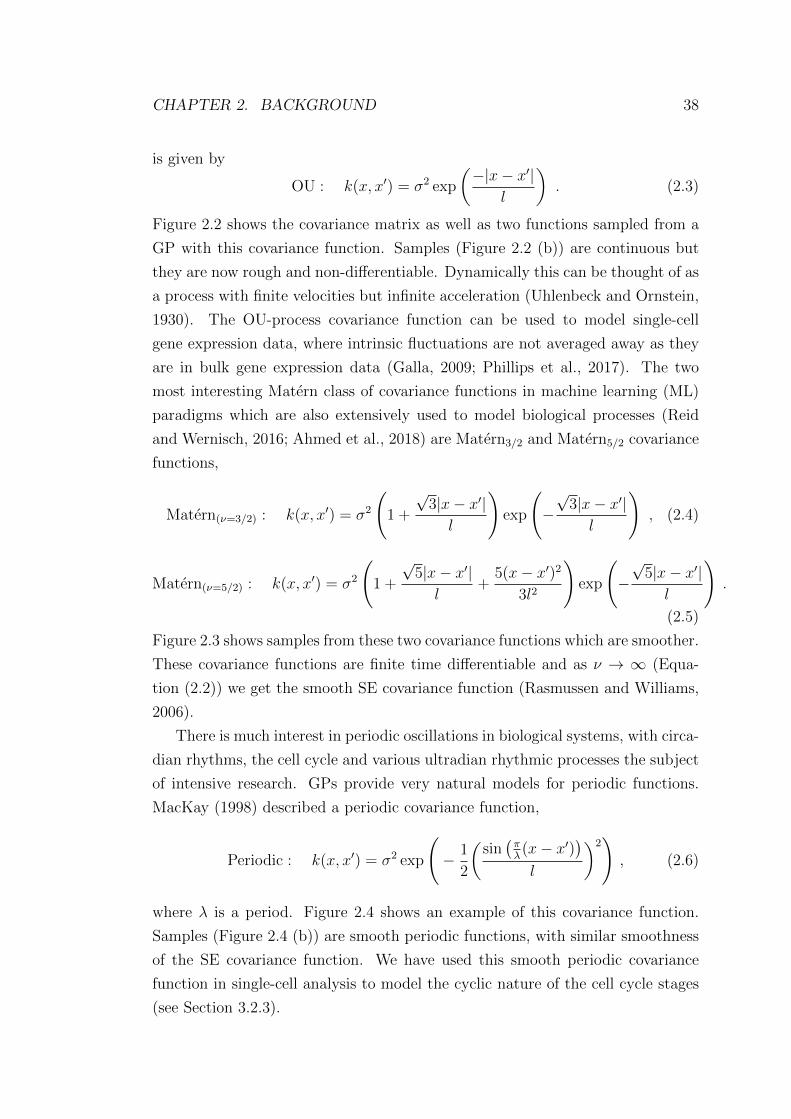
Figure 2.2 shows the covariance matrix as well as two functions sampled from a
GP with this covariance function. Samples (Figure 2.2 (b)) are continuous but
they are now rough and non-differentiable. Dynamically this can be thought of as
a process with finite velocities but infinite acceleration (Uhlenbeck and Ornstein,
1930). The OU-process covariance function can be used to model single-cell
gene expression data, where intrinsic fluctuations are not averaged away as they
are in bulk gene expression data (Galla, 2009; Phillips et al., 2017). The two
most interesting Matern class of covariance functions in machine learning (ML)
paradigms which are also extensively used to model biological processes (Reid
and Wernisch, 2016; Ahmed et al., 2018) are Matern3/2 and Matern5/2 covariance
functions,
Matern(ν=3/2) : k(x, x′) = σ2
(1 +
√3|x− x′|l
)exp
(−√
3|x− x′|l
), (2.4)
Matern(ν=5/2) : k(x, x′) = σ2
(1 +
√5|x− x′|l
+5(x− x′)2
3l2
)exp
(−√
5|x− x′|l
).
(2.5)
Figure 2.3 shows samples from these two covariance functions which are smoother.
These covariance functions are finite time differentiable and as ν → ∞ (Equa-
tion (2.2)) we get the smooth SE covariance function (Rasmussen and Williams,
2006).
There is much interest in periodic oscillations in biological systems, with circa-
dian rhythms, the cell cycle and various ultradian rhythmic processes the subject
of intensive research. GPs provide very natural models for periodic functions.
MacKay (1998) described a periodic covariance function,
Periodic : k(x, x′) = σ2 exp
(− 1
2
(sin(πλ(x− x′)
)l
)2), (2.6)
where λ is a period. Figure 2.4 shows an example of this covariance function.
Samples (Figure 2.4 (b)) are smooth periodic functions, with similar smoothness
of the SE covariance function. We have used this smooth periodic covariance
function in single-cell analysis to model the cyclic nature of the cell cycle stages
(see Section 3.2.3).

CHAPTER 2. BACKGROUND 39
x
x
(a)
f(x)
x
(b)
Figure 2.2: Illustration of the OU-process covariance function. The input setis generated by using a discretisation of the x-axis and contains 500 evenly dis-tributed points within the range [0, 20] . As this covariance function is very rough,we have used more input points to get an accurate path. The kernel hyperpa-rameters used are σ2 = 1 and l = 2 . (a) Covariance matrix. (b) Two randomfunctions drawn from a Gaussian process.
f(x)
x
(a) Matern3/2
f(x)
x
(b) Matern5/2
Figure 2.3: Samples from the two most popular Matern class of covariancefunctions. The input set is generated by using a discretisation of the x-axisand contains 200 evenly distributed points within the range [0, 20] . The kernelhyperparameters used are σ2 = 1 and l = 2 .

CHAPTER 2. BACKGROUND 40
x
x
(a)
f(x)
x
(b)
Figure 2.4: Illustration of the smooth periodic covariance function. The inputset is generated by using a discretisation of the x-axis and contains 500 evenlydistributed points within the range [0, 20] . The kernel hyperparameters are setto σ2 = 1, l = 0.5 and λ = 7 . (a) Covariance matrix. (b) Two random functionsdrawn from a Gaussian process.
The strong smoothness and absolute periodicity assumptions of the standard
periodic covariance function (Equation (2.6)) may not be a suitable choice for
many biological processes, thus the quasi-periodic OU process covariance func-
tion (Westermark et al., 2009) is used in relevant studies (see Rattray et al.
(2019) for a brief review).
Quasi-periodic OU : k(x, x′) = σ2 exp
(−|x− x
′|l
)cos
(|x− x′|lcos
). (2.7)
Here, the OU process covariance function (Equation (2.3)) is multiplied by a
Cosine covariance function where lcos is the lengthscale (determining the period)
of the Cosine covariance function. This is a simple example of how two kernels
can be combined to produce a new one (for more information, see Rasmussen
and Williams (2006)). Figure 2.5 shows the covariance matrix and a couple
of functions sampled from a GP with the quasi-periodic OU process covariance
function. The samples (Figure 2.5 (b)) are rough and approximately periodic
but oscillations gradually shift in phase over time so that they are not precisely
periodic. Phillips et al. (2017) used GP inference to identify stochastic oscillations
in single-cell microscopy data by fitting a GP model with the quasi-periodic OU
process covariance function.

CHAPTER 2. BACKGROUND 41
x
x
(a)
f(x)
x
(b)
Figure 2.5: Illustration of the quasi-periodic OU-process covariance function.The input set is generated by using a discretisation of the x-axis and contains200 evenly distributed points within the range [0, 20] . The process variance is setto σ2 = 1, the lengthscale of the OU-process covariance function and the Cosinecovariance function are set to l = 2 and lcos = 2/π respectively . Using units of πfor the lengthscale of the Cosine covariance function makes the kernel consistentwith the smooth periodic kernel (Equation (2.6)). (a) Covariance matrix. (b)Two random functions drawn from a Gaussian process.
The covariance functions we discussed above are all stationary, as they only de-
pend on the distance between time points x−x′. This stationarity assumption can
break down in certain applications. For example, gene expression time course data
may be collected after a perturbation leading to a rapid initial transient phase
before settling down to a constant value asymptotically. Non-stationary alterna-
tives have therefore been developed which can better model changes in amplitude
or lengthscale of gene expression data over time (see e.g. Heinonen et al., 2014).
Choosing an appropriate candidate set of covariance functions can be done
using application domain knowledge while statistical model selection can be used
to select the best one from this candidate set. For example, the roughness or
periodicity properties of a system may be suggested from first principles mod-
elling (Phillips et al., 2017) or the experimental design may suggest a hierarchical
data structure (Hensman et al., 2013). The automatic statistician (Duvenaud
et al., 2013) performs an automatic search over the space of covariance functions
and has some heuristics to pick the best one. Statistical model selection can
then be addressed using standard likelihood-based or Bayesian model selection
strategies, with recent methods to estimate out-of-sample prediction accuracy

CHAPTER 2. BACKGROUND 42
showing great promise (Vehtari et al., 2017). A nice feature of GP models is that
the sample paths can be analytically integrated out to obtain a marginal likeli-
hood that depends on relatively few parameters (see Section 2.2.2). This is an
attractive feature of GPs for both maximum likelihood and Bayesian integration
approaches, since there are relatively few parameters to optimise or integrate over
using numerical methods.
2.2.2 GP regression
Given a finite set of noise-corrupted measurements at different times, we are
interested in which underlying functions are most likely to have generated the
observed data. If we assume that the covariance function is known then this is
very easy to do with a GP, because we can condition and marginalise exactly
with Gaussian distributions.
In the regression setting, we have a data set D with regressors X = {xn}Nn=1
and corresponding real-valued targets Y = {yn}Nn=1. In the case of time course
data then the regressors are an ordered vector such that xn ≥ xn−1 but there is no
restriction on the spacing since GPs operate over a continuous domain. We allow
the case xn = xn−1 since that provides a simple way to incorporate replicates. We
assume that measurement noise in Y, denoted by ε, is independently Gaussian
distributed ε ∼ N (0, σ2noiseI) with variance σ2
noise and the underlying model for Y
as a function of X is f(·), so that
Y = f(X) + ε, (2.8)
where f(X) represents a sample from a GP evaluated at all the times in the
vector X. Our prior modelling assumption is that the function f is drawn from
a GP prior with zero mean and covariance function k(x, x′). The probability of
the data Y under the model is obtained by integrating out the function f(X),
p(Y|X) =
∫N (Y|f , σ2
noiseI)N (f |0, KNN) df
= N (Y|0, KNN + σ2noiseI) , (2.9)
where we have written f = f(X) and KNN = k(X,X) is the N × N covariance
matrix with elements k(xp, xq) determined by the covariance function k .

CHAPTER 2. BACKGROUND 43
A typical regression analysis will be focused on a new input x∗ and its pre-
diction f∗. Based upon Gaussian properties (Rasmussen and Williams, 2006) the
posterior distribution of f∗ given data Y is f∗|Y ∼ N (µ∗, C∗) with
µ∗ = k(X, x∗)>(KNN + σ2
noiseI)−1Y,
C∗ = k(x∗, x∗)− k(X, x∗)>(KNN + σ2
noiseI)−1k(X, x∗) ,
where k(X, x∗) is the N × 1 matrix of covariances evaluated between the training
input set X and the new test input x∗ and k(x∗, x∗) is the covariance evaluated
for the new input x∗ .
This is the posterior prediction of the function f at a specific time point x∗ but
is easily generalised to the full functional posterior distribution, showing that the
posterior function is another GP (Rasmussen and Williams, 2006). We see above
that the mean prediction is a weighted sum over data with weights larger for
nearby points in a manner determined by the covariance function. The posterior
covariance captures our uncertainty in the inference of f∗ which will typically be
reduced as we incorporate more data. Figure 2.6 shows an example of regression
with a squared exponential covariance function. In Figure 2.6 (a) we show some
samples from the prior and Figure 2.6 (b) is the posterior distribution fitted to
four observations. In this case, the data are observed without noise (σ2noise = 0)
but we still have uncertainty because many functions are consistent with the data.
The posterior shows which functions are likely given the data and our prior belief
in the underlying function. The prior expects functions to be smooth and not
to change very rapidly, and therefore our uncertainty increases gradually as we
move away from the data.
We often refer to the parameters of the covariance function (including the noise
variance) as hyper-parameters, since the function f(x) itself can be considered a
functional parameter of the model. The log-likelihood of the hyper-parameters
L(θ) is the logged probability of the data in Equation (2.9),
L(θ) = logN (Y|0, KNN + σ2I)
= −N2
log (2π)− 1
2log∣∣σ2
noiseI +KNN
∣∣− 1
2Y>(σ2
noiseI +KNN)−1Y .
(2.10)
This likelihood function has a complex form and may be multimodal so that

CHAPTER 2. BACKGROUND 44
f(x)
x
(a) Prior
f(x)
x
(b) Posterior
Figure 2.6: GP regression: (a): Ten samples drawn from a GP with a squaredexponential covariance function with hyper-parameters α = 1 and l = 1. (b):Five samples from the posterior distribution after observing four data pointswithout any observation noise (σ2
noise = 0). The functions are constrained topass through the data but the posterior distribution captures the uncertaintyaway from the data. The shading shows two standard deviations of posteriordistribution at each time.
hyper-parameter inference by either maximum likelihood or Bayesian inference
requires numerical optimisation or integration methods such as gradient decent
or Markov Chain Monte Carlo (MCMC).
However, the most common practical limitation of GPs in practice is the com-
putation required for inference; for each optimisation step the algorithm requires
O(N3) time and O(N2) memory, where N is the number of training examples.
Thus, to make the model computationally tractable, specially for large datasets,
a variety of sparse approximations have been proposed (Quinonero-Candela and
Rasmussen, 2005).
2.2.3 Sparse GP regression
Sparse approximations are useful techniques for practical inference of Gaussian
processes (GP) to deal with large datasets. Sparse approximations rely on a
small number of parameters termed inducing or auxiliary points that approxi-
mate the posterior distribution over functions. Sparse GP approximations reduce
the complexity to O(NM2), where M � N is the number of inducing points.

CHAPTER 2. BACKGROUND 45
The inducing points may be chosen from the training dataset or be an arbitrary
set such as a uniform grid in the input space. Further they may be treated as
constant or be optimised with respect to the model likelihood. The two most pop-
ular inducing point approximations for GPs are the Fully Independent Training
Conditional (FITC) (Snelson and Ghahramani, 2006) and the Variational Free
Energy approximation (VFE) (Titsias, 2009). The two methods differ in both
theoretical aspects as well as how the inducing points are handled.
Both methods can be succinctly summarized by a different parametrisation
of the marginal likelihood bound:
Ls(θ) = −N2
log(2π)− 1
2log |QNN +G|︸ ︷︷ ︸
complexity penalty
− 1
2Y> (QNN +G)−1 Y︸ ︷︷ ︸
data fit
− 1
2σ2noise
tr(T )︸ ︷︷ ︸trace term
.
(2.11)
For the VFE approximation we have
QNN = KNMK−1MMKMN , (2.12)
GVFE = σ2noiseIN , (2.13)
TVFE = KNN −QNN , (2.14)
where QNN is approximating the true covariance matrix KNN , but only involves
the inversion of a M ×M matrix KMM . KMM is the covariance matrix on the
inducing inputs Z; KNM is the cross covariance matrix between the training and
inducing inputs, i.e. between X and Z and KMN = KTNM .
The objective function of Equation (2.11) consists of three terms: the data fit
term imposes a penalty on data not well explained by the model; the complexity
term characterises the volume of probable datasets which are compatible with the
data fit term and therefore penalises complex models fitting well on only a small
ratio of datasets. Finally, the trace term measures the additional error due to the
sparse approximation. Without this term VFE may overestimate the marginal
likelihood as with previous methods of sparse approximation such as FITC. In
fact, the objective function of the FITC can be obtained from Equation (2.11)

CHAPTER 2. BACKGROUND 46
by using the same expression for QNN and taking
GFITC = diag [KNN −QNN ] + β−1IN , (2.15)
TFITC = 0, (2.16)
which clearly shows that the objective function of the FITC can be obtained by
modifying the GP prior
p(f |U) = N (f |0, QNN + diag [KNN −QNN ]) , (2.17)
where U are the inducing or auxiliary points.
In FITC, the inducing points are acting as an extra set of hyperparameters
to parametrise the covariance matrix QNN . As this approach changes the prior,
the continuous optimisation of the latent variable f with respect to the inducing
points U does not guarantee to approximate the full GP posterior (Titsias, 2009).
Moreover, as f is heavily parametrised because of the extra hyperparameter U
and the trace term is 0, overfitting may arise at the time of jointly estimating the
inducing points and hyperparameters. For both the VFE and FITC approxima-
tions, the inducing points may be chosen randomly from the training inputs or
optimized with respect to the marginal likelihood bound (for the detailed deriva-
tion of the bound as well as a more detail discussion of FITC and VFE, see
Section A.1).
We have developed our methods using the VFE approximation that tries
to maximise a lower bound to the exact marginal likelihood in order to select
the inducing points and model hyperparameters jointly. It minimises the KL
divergence (Kullback and Leibler, 1951) between the variational GP and the full
posterior GP which allows it to avoid overfitting as well as to approximate the
exact GP posterior.
While working with the inducing point approach, we have found that when
the input dimension is low (e.g. pseudotime estimation from single-cell data), it
is often sufficient to have a relatively small number of inducing points. Recently
Burt et al. (2019) have described that the number of inducing points M can of-
ten grow slowly with N . They have shown that as the datasets grow larger, the
number of inducing points can grow slowly for the KL divergence between the
approximation and the posterior to become very small. For a common case of
GP regression with the squared exponential covariance function (Equation (2.1)),

CHAPTER 2. BACKGROUND 47
they prove that the number of inducing points M can grow logarithmically with
the number of data points N . If inputs are D-dimensional and Gaussian dis-
tributed, then M = O(logDN
)is sufficient. They have shown that sparse GP
models can approximate the posterior efficiently using a smaller number of induc-
ing points. They conclude that the computational requirements of GP modelling
grow manageably as data volume increases, hence GP frameworks will continue
to evolve to becoming practical tools for analysing larger datasets.
2.2.4 Gaussian process latent variable model
GPs can be used for dimensionality reduction of multivariate data by treating
the regressors X as parameters (or latent variables) to be inferred along with the
functions f(X). Recall the GP model in Equation (2.8). Consider a multivariate
GP regression model for many data dimensions yi, with i = 1 . . . D, each with
their own GP function fi,
yin = fi(xn) + εin .
In the case of pseudotime inference then X = [xn] is a vector but more generally it
will live in some low-dimensional space that we would like to project our data into.
We treat X as a latent variable that has to be inferred along with the functions fi
and associated covariance hyper-parameters. This is the Gaussian Process Latent
Variable Model (GPLVM) which is a popular probabilistic approach for non-linear
dimensionality reduction (Lawrence, 2005; Titsias and Lawrence, 2010).
The log-likelihood can be worked out similarly to standard GP regression in
Equation (2.10), except that X is now a parameter of the model,
L(θ,X) = −ND2
log (2π)− D2
log∣∣σ2
noiseI +KNN
∣∣− 12tr[(σ2
noiseI +KNN)−1YY>],
(2.18)
where KNN has elements k(xp, xq) that depend on X through the covariance
function. In the original formulation of the GPLVM the latent points X were op-
timised by Maximum Likelihood (Lawrence, 2005) but later the Bayesian GPLVM
was introduced which placed a prior on X and a variational Bayesian inference
algorithm was used to approximate the posterior distribution over the latent
space (Titsias and Lawrence, 2010)(see Section A.2).

CHAPTER 2. BACKGROUND 48
2.2.5 Overlapping mixture of Gaussian processes
A mixture of GPs can be used for association problem, i.e. labelling data points
based on the latent functions that generate them. The overlapping mixture of
Gaussian processes (OMGP) (Lazaro-Gredilla et al., 2012) is a mixture model
where each mixture component corresponds to a latent GP function, and data
points at any time point can be allocated to any of these mixture components.
If data are multivariate and there are Mf different latent GP functions, then
F = {F1, F2, ..., FD} where Fd = {f1d, ..., fMf
d} and each fdm represents the latent
function associated with trajectory m for output dimension d. The OMGP uses
a N ×Mf binary associator matrix Z that defines the association between ob-
servations and latent functions where each row of Z can have only one non-zero
entry. The model needs to infer Z along with the set of latent functions F and
covariance hyperparameters θ. The model’s log-likelihood becomes
L(θ,F, Z) = logN(Y|ZF, σ2
noiseI)
= −ND2
log(2πσ2noise)−
1
2σ2noise
D∑d=1
(Yd − ZFd)> (Yd − ZFd) , (2.19)
where Yd is the observations for output dimension d. Unfortunately this log-
likelihood is not mathematically tractable as it needs to integrate out Z. Lazaro-
Gredilla et al. (2012) used non-standard variational inference algorithms (King
and Lawrence, 2006; Lazaro-Gredilla and Titsias, 2011) and derived a variational
collapsed lower bound to approximate the posterior (see Section B.1).
2.2.6 Gaussian process software packages
Gradient-based methods for optimisation (e.g. quasi-Newton or conjugate gradi-
ent) or Bayesian inference (e.g. Hamiltonian Monte Carlo, HMC) are imple-
mented in a number of popular GP inference software packages such as the
python packages GPy (GPy, since 2012), GPflow (Matthews et al., 2017), Gpy-
torch (Gardner et al., 2018) as well as the MATLAB libraries GPML (Rasmussen
and Nickisch, 2010) and GPstuff (Vanhatalo et al., 2013).
We have implemented our methods within the GPflow package that uses Ten-
sorFlow for its core computations, thus the inference can be performed in parallel
across multiple CPU cores and GPUs. Variational inference (VI) is the primary

CHAPTER 2. BACKGROUND 49
approximation method used in GPflow. The package is well tested and can pro-
vide accurate calculations for approximate inferences. GPflow supports the sparse
variational techniques and hence ensures scalable approximations, which we have
found very useful. Moreover, automatic differentiation support of GPflow simpli-
fies the model implementation by removing the extra burden of reimplementing
gradients. Finally, unlike other implementations of GP that assume an uninfor-
mative prior, the flexible architecture of GPflow package allows us to incorporate
prior knowledge in the form of an informative prior (see Chapter 3).
2.3 Gaussian process methods for single-cell data
One major drawback of the methods described in Section 2.1.1 is the absence
of an explicit probabilistic framework. They only provide a single point esti-
mate of pseudotime, concealing the impact of biological and technical variabil-
ity. Thus, the inherent uncertainty associated with pseudotime estimation is not
propagated to the downstream analysis and its consequences remain unknown.
While it may seem possible to develop probabilistic versions of these algorithms
with sufficient work, these algorithms will be mathematically intractable and
computationally infeasible1. Gaussian process (GP) inference provides a flexible
nonparametric probabilistic modelling framework that can be applied to single-
cell high-dimensional snapshot expression data for pseudotime estimation and for
gene-specific branching identification.
2.3.1 Pseudotime inference
The robustness of the estimated pseudotime for the models described in Sec-
tion 2.1.1 can be examined by re-estimating the pseudotimes multiple times under
different initial conditions, parameter settings or samples of the original data. For
instance, Campbell and Yau (2016) have examined the pseudotime estimation of
Monocle where they have taken multiple random subsets of data and re-estimated
the pseudotimes for each of them. They have shown that the pseudotime points
assigned by Monocle for the same cell can vary significantly across the random
subsets taken. This uncertainty in pseudotime assignment motivates the use of
probabilistic analysis techniques. The GPLVM is a non-linear probabilistic model
1See Randomized algorithm (en.wikipedia.org/wiki/Randomized_algorithm) to learnhow to introduce a degree of randomness to a non-probabilistic or deterministic algorithm.

CHAPTER 2. BACKGROUND 50
for dimension reduction (Lawrence, 2005) and has been used extensively to anal-
yse single-cell data. Buettner and Theis (2012) used the GPLVM for non-linear
dimension reduction to uncover the complex interactions among differentiating
cells. Buettner et al. (2015) used the GPLVM to identify subpopulations of
cells where the algorithm also dealt with confounding factors such as cell cycle.
More recently, Bayesian versions of the GPLVM have been used to model pseu-
dotime uncertainty. Campbell and Yau (2016) have proposed a method using the
GPLVM to model pseudotime trajectories as latent variables. They used Markov
Chain Monte Carlo (MCMC) to draw samples from the posterior pseudotime
distribution, where each sample corresponds to one possible pseudotime ordering
for the cells with associated uncertainties.
As well as allowing for uncertainty in inferences, Bayesian methods have the
advantage of allowing the incorporation of additional covariates which can inform
useful dimensionality reduction through the prior. In particular, pseudotime es-
timation methods may usefully incorporate capture times which may be available
from a single-cell time series experiment. For example, in the immune response
after infection, gene expression profiles show a cyclic behaviour which makes it
challenging to estimate a single pseudotime. Zwiessele and Lawrence (2016) used
the Bayesian GPLVM framework to estimate the Waddington landscape using
single-cell transcriptomic data; the probabilistic nature of the model allows for
more robust estimation of the topology of the estimated epigenetic landscape.
Reid and Wernisch (2016) have developed DeLorean, a Bayesian approach
that uses a GPLVM with a prior structure on the latent dimension. The latent
dimension in their model is a one-dimensional pseudotime and the prior relates
it to the cell capture time. This helps to identify specific features of interest such
as cyclic behaviour of cell cycle data. The pseudotime points estimated by their
model are in proximity to the actual capture time and use the same scale. Further,
Lonnberg et al. (2017) have adopted this approach and used sample capture time
as prior information to infer pseudotime in the their trajectory analysis. DeLorean
was applied on three different datasets from three different organisms collected
using different protocols (Windram et al., 2012; Shalek et al., 2014; McDavid
et al., 2014) where the model successfully estimated pseudotemporal ordering of
cells as well as cell cycle stages.
However, although the Bayesian GPLVM provides an appealing approach for
pseudotime estimation with prior information, existing implementations are too

CHAPTER 2. BACKGROUND 51
computationally inefficient for application to large single-cell datasets, e.g. from
droplet-based RNA-Seq experiments. In Chapter 3, we develop a new efficient
implementation of the Bayesian GPLVM with an informative prior which allows
for application to much larger datasets than previously considered.
2.3.2 Differential expression and branching
Lonnberg et al. (2017) developed GPfates that models cell differentiation towards
multiple fate decisions as well as supporting downstream analysis. The trajec-
tory inference in GPfates is a three-step procedure. First, the lower dimensional
representation of the data is achieved using a non-linear dimension reduction
algorithm GPLVM (Lawrence, 2005). Second, the model estimates pseudotime
for each cell. GPfates uses the Bayesian GPLVM with the informative prior ap-
proach motivated by the DeLorean model (Reid and Wernisch, 2016). Finally, the
algorithm uses the Overlapping Mixture of Gaussian Processes (OMGP) (Lazaro-
Gredilla et al., 2012) approach to assign cells to different branches. OMGP is a
collection of mixture components and each observation is assigned to one of these
components. In the single-cell paradigm, the observations are the cells and the
transcriptional state of a cell can be represented by the expression profiles of
all genes, a single gene, or a lower dimensional projection of the data. In GP-
fates, each mixture component corresponds to a different lineage. In the standard
OMGP, each component spreads throughout the entire (pseudo)time domain, but
in the case of branching structure, all components or lineages are identical before
the branching point (trunk state) and are different after the branching points.
GPfates uses this concept. Initially, from the starting of pseudotime, GPfates
considers the cells are in the trunk state and by setting the probability of cells
belonging to each branch to 0.5, the model converges to similar latent functions
in the trunk. The algorithm proceeds through the pseudotime and identifies the
event as a branching point where the likelihood experiences a sharp fall. GP-
fates employs a change point model to perform this analysis. In Chapter 4, we
introduce alternative branching models that strictly enforce the functions to be
identical before branching.
Once the trajectory inference is performed, GPfates uses the OMGP model
fit for downstream analysis. For each gene, GPfates creates a new model using
the fitted parameters and calculates the marginal likelihood of the model where
the transcriptional state of a cell is replaced with the individual gene expression.
CHAPTER 2. BACKGROUND 52
This model represents the gene bifurcating. GPfates then creates another model
for the same gene using arbitrary parameter values and calculates the marginal
likelihood. This model represents the gene not bifurcating. GPfates then com-
pares the likelihoods from these models which is eventually indicative whether
the gene expression is differentially expressed across the lineages.
GPfates also supports the identification of a gene-specific branching location.
It follows a similar approach of inferring global branching time, but instead of
using the transcriptional state of cells, it uses the individual gene expression.
GPfates was used to study the differentiation of CD4+ T cells into functionally
separate T helper cells where GPfates reconstructed the molecular trajectories
related to the development of Th1 and Tfh helper cells during blood-stage in
Plasmodium infected mouse.
However, the methods described here considers cell assignment to different
branches are fixed during downstream analysis. Recently, Boukouvalas et al.
(2018) have developed a non-parametric downstream analysis approach branch-
ing Gaussian process (BGP) that incorporates the associated cell assignment
uncertainty in the inference process (see Section 4.3). In this contribution, we ex-
tend the existing methodologies (e.g. Yang et al., 2016; Boukouvalas et al., 2018)
to work with single-cell resolution and provide efficient implementations that can
adequately identify DE genes as well as gene-specific branching locations.

CHAPTER 2. BACKGROUND 53
Table 2.1: An overview of some popular pseudotime and trajectory inferencemethods.
Met
hod
Ref
eren
ce
Pri
orre
quir
ed
Init
ial
DR
Cel
lor
der
ing
Pro
bab
ilis
tic
Bra
nch
ing
Monocle Trapnell et al. (2014) Yes ICA MST No Yes
Wanderlust Bendall et al. (2014) Yes NA KNN graph No Yes
Waterfall Shin et al. (2015) No PCA MST No No
TSCAN Ji and Ji (2016) No PCA MST No No
Embeddr Campbell et al. (2015) No Laplacian Principal curve No Noeigenmaps
SCUBA Marco et al. (2014) No tSNE Principal curve No Yes
Oscope Leng et al. (2015) No K- medoids Nearest No Noinsertion
Wishbone Setty et al. (2016) Yes NA KNN graph No Yes
DPT Haghverdi et al. (2016) Yes NA KNN graph No Yes
pseudogp Campbell and Yau (2016) No PCA GPLVM Yes No
DeLorean Reid and Wernisch (2016) Yes NA GPLVM Yes No
Monocle 2 Qiu et al. (2017a) Yes DDRTree MST No Yes
GPfates Lonnberg et al. (2017) Yes GPLVM GPLVM Yes Yes
Slingshot Street et al. (2018) Yes NA Principal curve No Yes
topslam Zwiessele and Lawrence (2016) Yes GPLVM KNN graph Yes Yes
GrandPrix* Ahmed et al. (2018) Yes NA GPLVM Yes Yes
Monocle 3 Cao et al. (2019) Yes UMAP AGA No Yes
* Method presented in this thesis.

Chapter 3
Scaling up probabilistic
pseudotime estimation
The Gaussian Process Latent Variable Model (GPLVM) is a popular approach
for dimensionality reduction of single-cell data and has been used for pseudotime
estimation with capture time information. However current implementations are
computationally intensive and will not scale up to modern droplet-based single-
cell datasets which routinely profile many tens of thousands of cells.
We provide an efficient implementation GrandPrix, which allows scaling up
this approach to modern single-cell datasets. We also generalize the application of
pseudotime inference to cases where there are other sources of variation, such as
branching dynamics. We apply our method on microarray, nCounter, RNA-seq,
qPCR and droplet-based datasets from different organisms. The model converges
an order of magnitude faster compared to existing methods whilst achieving sim-
ilar levels of estimation accuracy. Further, we demonstrate the flexibility of our
approach by extending the model to higher-dimensional latent spaces that can be
used to simultaneously infer pseudotime and other structures such as branching.
Thus, the model has the capability of producing meaningful biological insights
about cell ordering as well as cell fate regulation.
Availability: github.com/ManchesterBioinference/GrandPrix.
3.1 GrandPrix: Scaling up the Bayesian GPLVM
GrandPrix is motivated by the DeLorean approach (Reid and Wernisch, 2016)(de-
scribed in Section 2.3.1) and uses cell capture time to specify a prior over the
54

CHAPTER 3. PROBABILISTIC PSEUDOTIME ESTIMATION 55
pseudotime. The probabilistic nature of the model can be used to quantify the
uncertainty associated with pseudotime estimation. The GPLVM uses a Gaus-
sian process (GP) to define the stochastic mapping from a latent pseudotime
space to an observed gene expression space. A Gaussian process is an infinite
dimensional multivariate normal distribution characterised by a mean function
and a covariance function (see Section 2.2). In the GPLVM, the mean function
defines the expected mapping from the latent dimension to the observed data and
the covariance function describes the associated covariance between the mapping
function evaluated at any two arbitrary points in the latent space.
3.1.1 Model
The model we use is similar to the Bayesian GPLVM DeLorean model (Reid
and Wernisch, 2016); the main differences between the two approaches lie in how
model inference is accomplished which is discussed in Section 3.1.2. The primary
latent variables in our method are the pseudotimes associated with each cell. The
method expects the technical variability is sufficiently described by a Gaussian
distribution which is often accomplished by taking a logarithmic transformation of
the gene expression data (non-Gaussian likelihoods are investigated in Chapter
4). The critical assumption is that the cell capture times when available are
informative for the biological dynamics of interest. The capture time information
is not always available and the standard GPLVM (Lawrence, 2005) can be used
in the case of no prior information. However, in most biological experiments we
can argue there is usually some prior information. Even having bounds or some
rough idea of the order may be very useful as we have shown in our studies. The
log transformed expression profile of each gene yg is modelled as a non-linear
transformation of pseudotime which is corrupted by some noise ε
yg = fg(t) + ε, (3.1)
where ε ∼ N (0, σ2noise) is a Gaussian distribution with variance σ2
noise. We place
a Gaussian process prior on the mapping function
fg(t) ∼ GP (0, k(t, t′)) , (3.2)
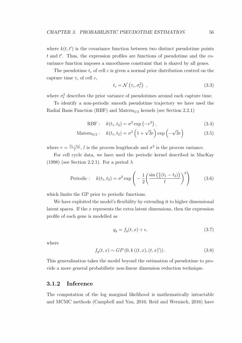
CHAPTER 3. PROBABILISTIC PSEUDOTIME ESTIMATION 56
where k(t, t′) is the covariance function between two distinct pseudotime points
t and t′. Thus, the expression profiles are functions of pseudotime and the co-
variance function imposes a smoothness constraint that is shared by all genes.
The pseudotime tc of cell c is given a normal prior distribution centred on the
capture time τc of cell c,
tc = N(τc, σ
2t
), (3.3)
where σ2t describes the prior variance of pseudotimes around each capture time.
To identify a non-periodic smooth pseudotime trajectory we have used the
Radial Basis Function (RBF) and Matern3/2 kernels (see Section 2.2.1)
RBF : k(t1, t2) = σ2 exp(−r2
), (3.4)
Matern3/2 : k(t1, t2) = σ2(
1 +√
3r)
exp(−√
3r)
(3.5)
where r = |t1−t2|l
, l is the process lengthscale and σ2 is the process variance.
For cell cycle data, we have used the periodic kernel described in MacKay
(1998) (see Section 2.2.1). For a period λ
Periodic : k(t1, t2) = σ2 exp
(− 1
2
(sin(πλ(t1 − t2)
)l
)2)
(3.6)
which limits the GP prior to periodic functions.
We have exploited the model’s flexibility by extending it to higher dimensional
latent spaces. If the x represents the extra latent dimensions, then the expression
profile of each gene is modelled as
yg = fg(t, x) + ε, (3.7)
where
fg(t, x) ∼ GP (0, k ((t, x), (t, x)′)) . (3.8)
This generalisation takes the model beyond the estimation of pseudotime to pro-
vide a more general probabilistic non-linear dimension reduction technique.
3.1.2 Inference
The computation of the log marginal likelihood is mathematically intractable
and MCMC methods (Campbell and Yau, 2016; Reid and Wernisch, 2016) have

CHAPTER 3. PROBABILISTIC PSEUDOTIME ESTIMATION 57
previously been employed for inference. Reid and Wernisch (2016) also use black
box variational approach to integrate over fg(t) that relies on data subsampling to
increase inference efficiency but they still use MCMC for the latent time sampling.
For the Bayesian GPLVM an analytic exact bound for variational inference over
both the GP functions and the latent points exists (Titsias and Lawrence, 2010;
Damianou et al., 2016) but the original derivation and all currently available
packages such as GPy (since 2012) assume an uninformative prior1. We modify
the exact bound to allow for informative priors
log p (Y ) ≥ Eq(t) [log p (Y |t)]−KL [q (t) ||p (t)] (3.9)
where q (t) is the variational distribution and
p (t) =N∏n=1
N(tn|τn, σ2
t
), (3.10)
is the modified prior centred at the capture time τn of cell n with prior variance
σ2t . The capture time prior variance σ2
t should be chosen with care. It should be
large enough so that the cells centred at capture time points τn are well spread
through the entire time course. Choosing a very small value for σ2t will narrow
down the search space of pseudotime orderings and will restrict the inference
process from discovering interesting regions. For a better result we recommend
that the mean of prior over the latent space should be scaled to the interval [0, 1]
and the prior variance can be chosen from the interval [0.1, 1]. We have also
found that a smaller capture time prior variance works better when the data has
more distinct capture time points and vice versa. We have examined the effect
of prior variance σ2t while working with the single-cell early developmental data
from mouse (Guo et al., 2010), which has 7 distinct capture time points, and we
have found that a smaller σ2t = 0.1 gives better results (see Section 3.2.6).
The variational approximation for the inputs q (t) is a factorised Gaussian as
in the standard Bayesian GPLVM (Titsias and Lawrence, 2010)
q (t) =N∏n=1
N(tn|τ ∗n, σ∗
2
t
). (3.11)
1It was true at the time of publishing GrandPrix (Ahmed et al., 2018), since then tools suchas Pyro (Bingham et al., 2019) have been developed to support informative prior.

CHAPTER 3. PROBABILISTIC PSEUDOTIME ESTIMATION 58
The modified lower bound on the model marginal likelihood is used to optimise
all model parameters including the kernel hyperparameters (process variance,
length scale, noise model variance) and the pseudotime locations. The Gaussian
assumption for the variational approximate distribution may fail to adequately
model multimodal distributions and model inference may be susceptible to local
optima, as different pseudotime orderings may provide similarly smooth expres-
sion profiles. Careful initialisation of the mean τ ∗n of variational approximation
q (t) helps the algorithm to obtain good orderings (see Section A.2). Although
using a non-Gaussian distribution would be possible, it would require a more
complex approximate inference scheme (Rasmussen and Williams, 2006). In our
experiments we find the estimated pseudotime ordering to be in close agreement
with known times as reflected by high rank correlation values.
The naive implementation of the Bayesian GPLVM has computational com-
plexity of O(GC3), where G is the number of genes and C is the number of
cells. Campbell and Yau (2016) have incorporated an MCMC implementation of
the Bayesian GPLVM without an approximation in their model and hence their
approach does not scale for large datasets. To make the model computationally
tractable for large datasets, we have adopted the Variational Free Energy (VFE)
sparse approximation (see Section 2.2.3). Sparse GP approximations reduce the
complexity to O(GCM2) where M � C is the number of auxiliary or inducing
points. These inducing points may or may not coincide with actual points. As
M is chosen much smaller than C, sparse approximations can result in significant
reductions in computational requirements.
To reduce computational complexity, Reid and Wernisch (2016) used the Fully
Independent Training Conditional (FITC) approximation (see Section 2.2.3).
This is a simple approach where a specific type of kernel is used to reduce the
computational requirement. The approach is attractive because only the kernel
is affected; the bound on the marginal likelihood is not affected and is therefore
simple to derive. However as Bauer et al. (2016) have shown, this approach is
prone to overfitting as it does not penalize model complexity. They recommend
use of the VFE approximation for GP regression where the bound of the marginal
likelihood is modified to include such a penalty term (see Section 2.2.3 for details).
Lastly, we have implemented our model in the GPflow package whose flexible
architecture allows to perform the computation across multiple CPU cores and
GPUs.

CHAPTER 3. PROBABILISTIC PSEUDOTIME ESTIMATION 59
Therefore, the source of the scalability of GrandPrix compared to DeLorean is
therefore three-fold: model estimation using an exact variational bound, a robust
sparse approximation (VFE vs FITC) and implementation on a scalable software
architecture.
3.2 Results and discussion
The performance of our model has been investigated by applying it on a num-
ber of datasets of varying sizes collected from different organisms using different
techniques. In all cases, GrandPrix converges quickly and uses a small number
of inducing points even for large datasets. First we have compared our method
with the DeLorean model (Reid and Wernisch, 2016) in terms of model fitting
as well as the time required to fit the model on all the datasets used by Reid
and Wernisch (2016); this encompasses the whole-leaf microarrays of Arabidopsis
thaliana (Windram et al., 2012); single-cell RNA-Seq libraries of mouse dendritic
cells (Shalek et al., 2014) and single-cell expression profiles of a human prostate
cancer cell line (McDavid et al., 2014). To reduce the effect of biological and
technical noise, Reid and Wernisch (2016) have used a similar approach of DE-
Seq (Anders and Huber, 2010), where they have calculated cell size based on a
subset of genes and a subset of cells and have used this cell size to normalise
the raw count data. We have downloaded these datasets from the DeLorean
package (Reid and Wernisch, 2016). As we are comparing our model with the
DeLorean model, we have used the same kernel function and capture time prior
variance as in Reid and Wernisch (2016) for these three datasets. Unlike the ap-
proach taken in Reid and Wernisch (2016) where the variational approximation is
computed numerically, our approach provides an exact analytical bound which,
as we show, results in robust parameter estimation. The results produced by our
model are similar to the DeLorean model, but our model converges significantly
faster. All the experiments have been carried out by using the same experimen-
tal setup, which is the same model structure and initial conditions. Overall, our
model outperforms the DeLorean model in both robustness and computational
scalability aspects.
We also apply our approach on more recent droplet-based single-cell data. We
apply the model on mouse embryo single-cell RNA-seq (Klein et al., 2015) and
compare our the predicted pseudotime with results from the diffusion pseudotime

CHAPTER 3. PROBABILISTIC PSEUDOTIME ESTIMATION 60
method (DPT) (Haghverdi et al., 2016). We then apply the model on a large
single-cell dataset of 3′
mRNA count data from peripheral blood mononuclear
cells (Zheng et al., 2017) to demonstrate scalability to tens of thousands of cells.
Finally, we demonstrate the flexibility of the model by applying it on single-
cell qPCR data of early development stages collected from mouse blastocyst (Guo
et al., 2010). We infer a two-dimensional latent space and show that the cap-
ture time used as an informative prior helps to disambiguate pseudotime from
branching structure.
3.2.1 Inferring withheld time points and smooth pseudo-
time trajectories
Windram et al. (2012) examined the effects of Botrytis cinera infection on Ara-
bidopsis thaliana. The time series were measured over 48 hours for both infected
and control conditions. The data contain 24 distinct capture time points where
the expression level of each time point is measured in 2 hour intervals. These
24 times points have been grouped into 4 separate groups, each consisting of 6
consecutive time points, which have been fed to the model for prior initialisation.
Thus the challenge was to infer the exact capture time for the samples when the
actual capture times were withheld.
The inference process uses the cells in the infected condition. Among the
150 genes described by Windram et al. (2012), we have used 100 genes for the
inference process. The remaining 50 genes were left out as held-out genes and
used further to validate the model as in Reid and Wernisch (2016). We have used
the Matern3/2 kernel (Equation (3.5)) and set the capture time prior variance
to σ2t = 9 as in Reid and Wernisch (2016). In Figure 3.1, we have plotted the
estimated pseudotime using 10 inducing points against the actual capture time
and it shows a close correspondence between these two quantities.
In Figure 3.2 we compare out model with the DeLorean model. Figure 3.2 (a)
shows the best and average, over 20 different initialisations, Spearman correlation
between the actual capture time and the estimated pseudotime as the number of
inducing points is increased. Both the best and average correlation values show
that our method has faster convergence for a smaller number of inducing points
than the DeLorean method2. Figure 3.2 (b) depicts the fitting time required by
2Both the best and average correlations led to the same values when ten or more inducingpoints are used.

CHAPTER 3. PROBABILISTIC PSEUDOTIME ESTIMATION 61
Tru
eca
ptu
reti
me
Pseudotime
Figure 3.1: Arabidopsis thaliana microarray data (Windram et al., 2012): Pseu-dotime posterior mean (horizontal axis) vs true capture time. Colours denote theprior information used by the GPLVM model.
both models for different number of inducing points. As our model uses the VFE
approximation with an exact bound, it converges an order of magnitude faster
than the DeLorean model which requires a sampling process for the latent points.
The problem with the sampling approach is that it requires initial burn-in time
to fit the model which makes the inference slower and therefore problematic for
larger datasets.
The means of the estimated pseudotime distribution from the DeLorean and
the GrandPrix models are in good agreement as evident from the Figure 3.2 (a).
Both models also possess similar posterior variance. The average standard devia-
tion of the 24 time points is 0.53 in the GrandPrix model and 0.54 in the DeLorean
ADVI model. The DeLorean MCMC model has a higher average sample standard
deviation (0.98). Having unlimited computational resources, the sample variance
of an MCMC algorithm is expected to approach the true posterior distribution
variance. It therefore seems likely that both variational algorithms are underes-
timating the posterior variance for this dataset. In scenarios where the posterior
variance over pseudotime is important, such as when assessing the uncertainty
of pseudotime assignments (Campbell and Yau, 2016), the potential underesti-
mation of the variance by both variational approaches means that the MCMC

CHAPTER 3. PROBABILISTIC PSEUDOTIME ESTIMATION 62
Sp
earm
anC
orre
lati
on
(a)
Number of inducing points
Fit
tin
gti
me
(s)
(b)
Number of inducing points
Figure 3.2: Arabidopsis thaliana microarray data (Windram et al., 2012): Acomparison of performance and fitting time between the proposed method andDeLorean method. (a): Spearman correlation between the actual capture timeand the estimated pseudotime for different number of inducing points. (b): Fit-ting time required by the models for the same experimental setups.

CHAPTER 3. PROBABILISTIC PSEUDOTIME ESTIMATION 63
approach would be preferable if it were computationally feasible. Unfortunately,
the DeLorean MCMC approach is not computationally feasible when the num-
ber of cells is larger than a few hundred (Saelens et al., 2018). The problem
with MCMC algorithms is that they need extremely long times to reach the de-
sired stationary distributions for large datasets and convergence time can increase
rapidly as the size of the dataset increases (Mossel et al., 2006). Moreover, in the
case of multimodal posterior distributions, the MCMC algorithms may quickly
converge to one of the modes and may fail to explore others even for smaller
datasets (Kucukelbir et al., 2015). There is no straightforward guideline to eval-
uate the accuracy and to examine convergence. Researchers use multiple Markov
chains to compare and examine the accuracy of convergence, which in the long
run increases the computational burden. A systematic study of the challenges
associated with the MCMC algorithms can be found in Mossel et al. (2006) and
a comprehensive comparison between VI and MCMC is available in Blei et al.
(2017).
Reid and Wernisch (2016) defined the roughness statistic Rg as the difference
of consecutive expression measurements under the ordering given by pseudotime
(see Section A.3). Our model estimates smooth pseudotime trajectories which
have close correspondence with the actual capture time points. To verify the
smoothness of our predicted trajectory, we calculated the roughness statistics for
the 50 held out genes. The average Rg for all experiments in Figure 3.2 is the
same for both the DeLorean and Bayesian GPLVM approaches (0.71), reflecting
the pseudotime similarity. Figure 3.3 shows the average Rg of our estimated
pseudotimes which shows the model’s potential to produce smooth trajectories
even when using a small number of inducing points.
3.2.2 Correctly identifying precocious cells
Shalek et al. (2014) investigated the primary bone-marrow-derived dendritic cells
of mouse in three different conditions. The time course data were collected using
single-cell RNA-seq technology. They described several modules of genes which
show different temporal expression patterns through the lipopolysaccharide stim-
ulated (LPS) time course. They identified a core antiviral gene module expressed
in LPS after 2-4 hours, and found two cells captured at the 1 hour mark which
switched to this group precociously. That is, these two cells have genes expressed
which are not expressed in the other cells of the 1 hour group. It reflects the

CHAPTER 3. PROBABILISTIC PSEUDOTIME ESTIMATION 64
Ave
rageRg
Number of inducing points
Figure 3.3: Arabidopsis thaliana microarray data (Windram et al., 2012): Av-erage roughness statistics of estimated pseudotime using GrandPrix for differentnumber of inducing points.
concept that some cells can progress faster through the differentiation process.
Thus the challenge is to assign these two precocious cells at a later pseudotime
than the other cells in the 1 hour group which will confirm the model’s capability
to uncover the developmental time line without being overly influenced by the
capture time prior information.
To fit the model, we have used 307 cells from the LPS time course which
includes the two precocious cells. Among the several gene modules, the inference
process used the top 74 most variably expressed genes from the clusters Id, IIIb,
IIIc, IIId as in Reid and Wernisch (2016). Here we have used the Matern3/2 kernel
(Equation (3.5)) and set the capture time prior variance to σ2t = 1 as in Reid and
Wernisch (2016). Figure 3.4 (a) shows the fitting of our model using 30 inducing
points for the mouse dendritic cell data. The module score (Shalek et al., 2014)
of core antiviral genes have been plotted over the estimated pseudotimes. Two
precocious cells have been assigned pseudotimes in the middle of the 2 hour group
rather than in the 1 hour group, which implies that the model correctly infers that
some cells can progress across the differentiation trajectory faster than others.
Figure 3.4 (b) depicts the fitting time required by the both models for differ-
ent number of inducing points and in all the cases the Bayesian GPLVM model
converges significantly faster than the DeLorean model.

CHAPTER 3. PROBABILISTIC PSEUDOTIME ESTIMATION 65
1
2
3
4
5
0 5Pseudotime
Mod
ule_
scor
e
typeNot precociousPrecocious
Capture TimeUnstimulated1hr2hr4hr6hr
(a)
Fit
ting
tim
e(s
)
(b)
Number of inducing points
Figure 3.4: Mouse dendritic cells (Shalek et al., 2014): (a): The module scoreof core antiviral cells over pseudotime. The two precocious cells (plotted astriangles) have been placed in later pseudotimes than the other cells capturedat 1 hour. A Lowess curve (solid blue line) has been plotted thorough the data.(b): Comparison of fitting time required by both the DeLorean and our modelsfor different number of inducing points while using the same experimental setups.

CHAPTER 3. PROBABILISTIC PSEUDOTIME ESTIMATION 66
3.2.3 Recovering cell cycle peak times
McDavid et al. (2014) examined the effect of cell cycle on single-cell gene expres-
sion across three human prostate cancer cell lines. They assayed the expression
profiles of 333 genes in 930 cells by using single cell nCounter. To model the
cyclic nature of the cell cycle, we have used a periodic kernel (Equation (3.6))
with a capture time prior variance σ2t = 1
4as in Reid and Wernisch (2016). This
ensures the modelling of periodicity in the gene expression corresponding to the
different cell cycle stages. We have used the expression data from the PC3 hu-
man prostate cancer cell line. The inference has been carried out by using the
top 56 differentially expressed genes in 361 cells. The cells identified as G0/G1,
S and G2/M by McDavid et al. (2014) have been mapped to the capture times
of 1, 2 and 3, respectively as in Reid and Wernisch (2016). Due to the additional
challenge of optimizing pseudotime parameters for periodic data, we follow the
approach of Reid and Wernisch (2016) where we have used as initial conditions
random pseudotimes having the largest log likelihood to estimate cell cycle peak
time points. Figure 3.5 shows the expression profiles of some selected genes over
the estimated pseudotime (using 20 inducing points).
The DeLorean model requires 7h 31m to fit the model while our method uses
20 inducing points and takes only 4m 45s to converge whilst achieving similar er-
ror in recovering the cell cycle peak times. The DeLorean approach uses samples
from 40 model initialisations to generate a full posterior GP whilst the BGPLVM
only requires a single initialization as an analytic bound of the marginal likeli-
hood is available. We also attempted to compare the fitting time required for
different numbers of inducing points for this dataset but the sparse kernel used in
the DeLorean packages results into non-invertible covariance matrices. Therefore
the sparse approximation followed in the DeLorean package appears more frag-
ile in cases of non-standard kernels such as the periodic kernel. The estimated
pseudotimes are in good agreement with the cyclic behaviour of the data.
The model also predicts the cell cycle peak time of each gene with similar ac-
curacy level of the DeLorean approach. In the CycleBase database (Santos et al.,
2014), the cell cycle related genes are arranged according to their peak times.
To evaluate the models performance, estimated peak times from the expression
profiles fit by our model have been compared with the peaks times defined by the
CycleBase database. The root mean square error (RMSE) between the estimated
peaks and the CycleBase defined peaks is similar to DeLorean model (∼14.5).

CHAPTER 3. PROBABILISTIC PSEUDOTIME ESTIMATION 67
Figure 3.5: Cell cycle data of PC3 human prostate cancer cell line (McDavidet al., 2014): Expression profiles over estimated pseudotime for some selectedgenes from PC3 human prostate cancer cell line. Each point corresponds to aparticular gene expression in a cell. The points are coloured based on cell cyclestages according to McDavid et al. (2014). The circular horizontal axis (whereboth first and last labels are G2/M) represents the periodicity realized by themethod in pseudotime inference. The solid black line is the posterior predictedmean of expression profiles while the grey ribbon depicts the 95% confidenceinterval. The vertical dotted lines are the CycleBase peak times for the selectedgenes.

CHAPTER 3. PROBABILISTIC PSEUDOTIME ESTIMATION 68
3.2.4 Recovering Diffusion Pseudotime (DPT)
To investigate the robustness and scalability of our method, we have applied it
on droplet-based single-cell data. First, we have applied the model on single-cell
RNA-seq data from mouse embryonic stem cells (ESC) generated using droplet
barcoding (Klein et al., 2015). Klein et al. (2015) developed a method termed
inDrop (indexing droplet) based on droplet microfluidics. They assayed the
gene expression profiles and differentiation heterogeneity of mouse stem cells af-
ter leukaemia inhibitory factor (LIF) withdrawal. They captured the cells at
t = 0, 2, 4 and 7 days and used their protocol to profile 2717 cells with 24175
observed transcripts. Haghverdi et al. (2016) have used this dataset for their
analysis of diffusion pseudotime (DPT). They have applied their model on the
cell cycle normalised data to infer DPT. Haghverdi et al. (2016) have normalised
the count data using library size and log transformation. They have used the
scLVM package (Buettner et al., 2015) for cell cycle normalisation and batch ef-
fects correction. We have used this cell cycle normalised data to assess the quality
of the Bayesian GPLVM inferred pseudotime.
The inference process uses 2717 cells and 2047 genes. The model uses a RBF
kernel (Equation (3.4)) to identify a smooth pseudotime trajectory. As cell cycle
and batch effects are corrected for this dataset, it should be less dependent on the
prior and therefore we have set the capture time prior variance to σ2t = 1. The
pseudotime estimated by our model has a high rank correlation with both the
actual capture time as well as the estimated pseudotime using DPT (Figure 3.6).
As memory is a crucial resource when analysing large volumes of data, we
also examine the effect of lower precision computations. We have examined the
performance of our model under both 64 and 32 bits floating point precision.
In both cases we observe a strong correlation with DPT (∼0.94) but note a
significant reduction in fitting time when using 32 bits precision. For 64 bits
precision the algorithm take ∼32 seconds to converge, whilst it takes only ∼11
seconds to converge for 32 bits precision.
Pseudotime inference without informative prior
We have also run the GrandPrix model without an informative prior. The esti-
mated pseudotime has a high rank correlation with both the actual capture time
(0.92) and the diffusion pseudotime (0.93). Although the rank correlation between

CHAPTER 3. PROBABILISTIC PSEUDOTIME ESTIMATION 69
Tru
eC
aptu
reti
me
(a) Correlation = 0.91
BGPLVM-1 ( Pseudotime)
Diff
usi
onP
seudot
ime
(DP
T)
(b) Correlation = 0.96
BGPLVM-1 ( Pseudotime)
Figure 3.6: Mouse embryonic stem cells (Klein et al., 2015): Comparison ofestimated pseudotime with the actual cell capture time and the pseudotime esti-mated using DPT. The points are coloured according to the actual cell capturetimes. The rank correlation is shown in the caption of each subplot.

CHAPTER 3. PROBABILISTIC PSEUDOTIME ESTIMATION 70
estimated pseudotime and diffusion pseudotime have similar values for both in-
formative priors (Figure 3.6(b)) and non-informative (Figure 3.7(b)), the model
with capture time as an informative prior shows a closer to linear correspondence
to DPT. This is reflected in a higher linear correlation for the informative prior
model (0.964) compared to the non-informative prior model (0.931).
3.2.5 2D visualization of ∼68k Peripheral Blood Mononu-
clear Cells (PBMCs)
We also apply our method on a larger single-cell RNA-seq dataset to further
demonstrate its scalability. Zheng et al. (2017) have presented a droplet-based
technology that enables 3′
messenger RNA (mRNA) digital counting to encapsu-
late tens of thousands of single cells per sample. In their method, reverse tran-
scription takes place within each droplet and barcoded complementary DNAs
(cDNAs) have been amplified in bulk. The resulting libraries are then used for
Illumina short-read sequencing. Their method has 50% cell capture efficiency and
can process a maximum of 8 cells simultaneously in each run. Zheng et al. (2017)
have assayed ∼68k peripheral blood mononuclear cells (PBMCs) demonstrating
the suitability of single-cell RNA-seq technology to characterise large immune cell
populations.
Zheng et al. (2017) first performed deduplication of reads based on UMI tags,
such that counts represent numbers of molecules. Then the UMI count data were
log-normalised and finally, the expression profile of each gene was normalised to
zero mean and unit standard deviation. In majority of the cases of single-cell
experiments, no external classification information is available and thus unsuper-
vised clustering approaches are typically applied to cluster the cells. Unsupervised
clustering or learning the grouping of a set of objects based on their similarity
without using any ground truth or data labels is challenging. At single-cell res-
olution, inherent technical, biological and computational challenges make the
problem even harder. Clustering algorithms depend on the measure of distances
between objects or data points. Single-cell RNA-seq data are high dimensional,
i.e. a larger number of genes are assayed from a larger number of cells. Moreover,
the data are noisy and the expression matrix contains a lot of zeros. There-
fore, differences between distances tend to be smaller and the algorithms may
fail to reliably partition cells into different groups or clusters. To de-noise the

CHAPTER 3. PROBABILISTIC PSEUDOTIME ESTIMATION 71
Tru
eC
aptu
reti
me
(a) Correlation = 0.92
BGPLVM-1 ( Pseudotime)
Diff
usi
onP
seudot
ime
(DP
T)
(b) Correlation = 0.93
BGPLVM-1 ( Pseudotime)
Figure 3.7: Mouse embryonic stem cells (Klein et al., 2015): GrandPrix hasbeen applied without using informative prior. The estimated pseudotime hasvery high correlations with the actual capture time as well as DPT, though theestimated pseudotime does not show similar density to DPT.

CHAPTER 3. PROBABILISTIC PSEUDOTIME ESTIMATION 72
data, feature selection and dimensionality reduction are used. However, linear
dimensionality reduction algorithms such as PCA fails to capture the complex
non-linear relationships between cells. On the other hand, non-linear dimension-
ality reduction algorithms such as tSNE and UMAP offer more flexibility but
requires the users to define parameter values which may greatly affect the projec-
tion of data into lower dimensional space. Moreover, most clustering algorithms
require the users to predefine the resolution of clustering. For instance, the most
popular clustering algorithm k-means needs users to set the number of clusters.
There are no principled or well accepted guidelines for choosing these user defined
parameters. Overestimating or underestimating these parameters may result in
misleading outcomes such as the algorithms may mistakenly consider random
noise as true structures (Kiselev et al., 2019). While the user assumes that each
cluster will represent a true distinct cell type, there is no ground truth or well
accepted fixed criteria. Considering the higher noise in single-cell data, it is very
difficult to distinguish between true biological clusters and technical artefacts.
A comprehensive study on available single-cell unsupervised clustering methods
and tools, associated challenges and opportunities can be found in Kiselev et al.
(2019).
Zheng et al. (2017) used the top 1000 differentially expressed genes ranked by
their normalised dispersion, a similar approach of (Macosko et al., 2015). First
they used PCA to identify the first 50 principal components, then applied the k-
means clustering algorithm and identified 10 distinct cell or cluster labels. They
used tSNE to visualise 10 cell clusters from k-means in a two-dimensional pro-
jection. We use a 2D GPLVM model with no capture time prior information and
an RBF kernel (Equation (3.4)). We use the same top 1000 variably expressed
genes ranked by their normalised dispersion by Zheng et al. (2017). The 2D la-
tent spaces from tSNE are used to initialise the model. We have used 60 inducing
points initialised via Latin Hypercube Sampling (LHS) (McKay et al., 1979; Lar-
son et al., 2005). LHS is a statistical method that gives a near random sample
from a multi-dimensional distribution. The inducing points and hyperparameters
have been optimised jointly with model parameters and the algorithm takes ∼10
minutes to converge on a simple desktop machine3.
3Intel(R) Core(TM) i5-3570 CPU @ 3.40GHz with 16 GB memory.

CHAPTER 3. PROBABILISTIC PSEUDOTIME ESTIMATION 73
Further we have investigated the scalability of the model across varying num-
ber of CPU cores4. For simplicity only the 1D latent positions are optimised,
using fixed values for the kernel hyperparameters l = 1 and σ2 = 1 and the in-
ducing points. In Figure 3.8 we show the time required per iteration when using
different number of CPU cores for both 32 and 64 bit precision. The computa-
tional benefit of lower precision is reduced as the number of cores is increased.
We also note the diminishing returns of increasing the number of CPU cores;
we see an approximately doubling of performance when increasing the number
of cores from 2 to 4 but a reduced benefit when increasing from 8 to 16. We
recommend a small number of cores is assigned to an individual model fitting,
with any remaining resources assigned to perform multiple model fittings using
different initial conditions. The latter is needed to alleviate the local minima
problem inherent when fitting a Bayesian GPLVM model.
Figure 3.8: PBMCs with ∼68k cells (Zheng et al., 2017): Time per iterationusing 1, 2, 4, 8, 16 CPU cores. The algorithm has been applied using both 32 and64 bit floating point precision.
We can further improve the computational performance of the GrandPrix
model by fixing rather than optimising the inducing point locations. This results
in faster convergence without sacrificing accuracy given a sufficient number of
inducing points is used. The effectiveness of this approach stems from the high
amount of redundancy that is typical in larger datasets and offers a way to scale
4The hardware used was a 16-core Intel Ivy Bridge CPUs (E5-2650 v2, 2.60GHz) with 512GB memory. TensorFlow version 1.0.0 and GPflow version 0.3.8.

CHAPTER 3. PROBABILISTIC PSEUDOTIME ESTIMATION 74
up the GrandPrix approach to datasets with a larger number of cells. Figure 3.9
shows the 2D Bayesian GPLVM visualisation of ∼68k PBMCs. Each cluster label
represents the corresponding clustering reported in Zheng et al. (2017). Figure 3.9
(a) shows the estimated latent dimensions from the model that optimises the
inducing points where as Figure 3.9 (b) corresponds to the model with fixed
inducing points.
To highlight the importance of sensible initialisation we have also used PCA
to initialise the model. Figure 3.10 shows a comparison of the adjusted rand
index (ARI) (Hubert and Arabie, 1985) values between the predicted clustering
from 2D Bayesian GPLVM model (initialised using both PCA and tSNE) and
the clustering reported in Zheng et al. (2017) for different number of inducing
points used. The ARI has a value near to 0.0 if the cluster labelling is performed
randomly and 1.0 for identical clusterings. In all the cases we have used the same
experimental setup as well as same initialisation of the inducing variables. The
model initialised using the tSNE consistently possesses better ARI values than
the model initialised with the PCA. Thus initialisation using the tSNE is helping
the model to discover better local optima.
The performance of VFE approximation is expected to improve with an in-
creasing number of inducing points. Figure 3.10 shows that as we use more
inducing points, we get a bigger ARI between the GrandPrix latent space clus-
tering and the clustering reported in Zheng et al. (2017). However, using more
inducing points requires extra memory and increases the number of model param-
eters. From Figure 3.9 and 3.10, we observe similar ARI values when optimising
or fixing the inducing point locations given a sufficient number of inducing points
(≥ 40 in this case). Thus when using more inducing points, optimising them
does not significantly improve the model performance in terms of the ARI be-
tween the clustering using estimated latent spaces and the clustering reported in
Zheng et al. (2017). Table 3.1 shows the number of iterations required by the
model to converge and Table 3.2 shows the time required for each iteration for
different number of inducing points. Using more inducing points improves the
performance and fixing them reduces the computational cost per iteration with-
out significantly affecting the number of iterations to convergence given enough
inducing points (≥ 40). Conversely, using a small number of inducing points fails
to represent the entire complexity of the system and it is beneficial to optimise
their location. However, the optimisation problem is very hard and non-convex.

CHAPTER 3. PROBABILISTIC PSEUDOTIME ESTIMATION 75
BG
PLV
M-2
(a) Optimizing inducing points
BGPLVM-1
BG
PLV
M-2
(b) Fixing inducing points
BGPLVM-1
Figure 3.9: PBMCs with ∼68k cells (Zheng et al., 2017): 2D visualisation, themodel is initialised using lower dimensional representation from tSNE and uses60 inducing points. (a): The model optimising the inducing points, has an ARI0.538. (b): The model without optimising the inducing points, has an ARI 0.532.Both models have similar level of ARI values, while the latter converges faster.The cell clusters from Zheng et al. (2017) are also shown.

CHAPTER 3. PROBABILISTIC PSEUDOTIME ESTIMATION 76
AR
Iva
lues
Number of inducing points
Figure 3.10: PBMCs with ∼68k cells (Zheng et al., 2017): Comparison of theARI values of the models initialised using the lower dimensional representationfrom both tSNE and PCA for different number of inducing points. The perfor-mance has been analysed by optimising as well as fixing the inducing points.
Local optima are a problem and the optimiser may end up with quite poor solu-
tions. When we are using 20 inducing points initialised using PCA, optimising
the inducing points is making the model converge to a bad local optima. We can
employ some heuristics such as random restarts to reduce the problem but there
are no guarantee that the model will always converge to a better local optima.
Table 3.1: Number of iterations to convergence required by the model initialisedusing tSNE to optimise 2D latent spaces from ∼68k PBMCs for different numberof inducing points. The number of iterations reported are for both the modelsoptimising and fixing the inducing points.
# inducing points 20 40 60
# iterations to converge: Optimizing inducing points 16 29 24
# iterations to converge: Fixing inducing points 56 27 28
Therefore, while working with larger datasets, the model must be initialised
sensibly and inducing point location may be fixed when a sufficient number is
used. Optimising inducing points jointly with model parameters and hyperpa-
rameters may find better minima but constraints on the available computational

CHAPTER 3. PROBABILISTIC PSEUDOTIME ESTIMATION 77
Table 3.2: Fitting time required per iteration by the model initialised usingtSNE to optimise 2D latent spaces from ∼68k PBMCs for different number ofinducing points.
Number of inducing points 20 40 60
Approx. time (s)/iter: Optimizing inducing points 4.2 10.1 24.0
Approx. time (s)/iter: Fixing inducing points 2.7 9.3 19.1
resources may make this impractical. Thus rather than optimising a small number
of inducing points, using more carefully initialised but fixed inducing points may
exhibit better performance. The inducing points can be chosen from a random
subset of the model parameters or from a random multidimensional distribution.
Additionally, if prior knowledge of the system is available, the number of induc-
ing points may be set sensibly, taking into account problem complexity such as
discontinuities, changepoints, etc.
3.2.6 Extending the model to infer pseudotime-branching
To demonstrate the flexibility of our approach, we extend the model to 2D latent
spaces with a capture time prior on one latent dimension and apply it on single-
cell qPCR data of early developmental stages in mouse (Guo et al., 2010). The
gene expression profiles of 48 genes were measured across 437 cells. Cells were
captured from single embryos at different times in mouse embryonic development.
At the 32-cell stage they begin to differentiate into three different cell states in
the 64 cell stage: trophectoderm (TE), epiblast (EPI), and primitive endoderm
(PE). Data normalisation step includes endogenous control genes. For each cell,
the average expression levels of endogenous reference genes Actb and Gapdh were
subtracted (Guo et al., 2010). We downloaded this dataset from python open
data science (pods) software repository (https://github.com/sods/ods). The
data were log normalised and transformed to zero mean and unit standard devi-
ation. We found that aligning one axis with time makes the latent space more
interpretable, with the other dimension capturing differences in cell type. In Fig-
ure 3.11, we see that the non-linear dimensionality reduction of the GPLVM leads
to a cleaner separation of cell stages and types compared to a linear approach
such as PCA.
Next, models with both informative and non-informative priors are examined
(Figure 3.12). Both models use an RBF kernel (Equation (3.4)). Both models are

CHAPTER 3. PROBABILISTIC PSEUDOTIME ESTIMATION 78
PC
-2
PC-1
(a) PCA
BG
PLV
M-2
BGPLVM-1(Pseudotime)
(b) Bayesian GPLVM
Figure 3.11: Single-cell qPCR of early developmental stages (Guo et al., 2010):The single-cell gene expression data are projected onto two latent dimensionsusing PCA and the Bayesian GPLVM with prior mean in one latent dimensionbased on capture times.

CHAPTER 3. PROBABILISTIC PSEUDOTIME ESTIMATION 79
initialized with identical values. For the informative prior, we set the capture time
variance to σ2t = 0.1. The informative prior (Figure 3.12 (b)) on capture time
helps with the identifiability of the model as it aligns the first latent dimension
(horizontal axis) with pseudotime and the second latent dimension (vertical axis)
with the branching structure.
To investigate how the branching dynamics affect the estimation of pseudotime
points, we have used our model to infer the 1D pseudotimes with informative
prior and compared it with the pseudotimes from the 2D informative prior model
(Figure 3.13 (a) and (b)). Both models were run from multiple initial conditions
to ensure a good likelihood optimum was obtained. The 2D model estimate of
the pseudotime is found to have better correspondence with the actual capture
time (Spearman correlation 0.84 vs 0.95), suggesting that the 1-D model is less
able to align all variation with a pseudotime axis.
We have used the estimated pseudotime to visualise changes in the gene ex-
pression levels while the cells are progressing through differentiation stages. In
Figure 3.14, we have plotted the expression profiles of two marker genes against
our estimated pseudotime points. Id2 is a known marker gene for TE, thus it
behaves differently in TE cells from the other two differentiation stages. It is dif-
ferentially expressed between the stages TE and EPI, as well as between TE and
PE (Figure 3.14 (a)). Similarly, Figure 3.14 (b) shows that Sox2 is differentially
expressed between the stages TE and EPI, and between the stages PE and EPI.
Zwiessele and Lawrence (2016) have listed genes that were differentially ex-
pressed for each pair of cell states, i.e. TE and EPI; PE and EPI; TE and PE.
They listed the top 10 differentially expressed genes for each cell type transition.
The marker genes of each cell type transition identified by Zwiessele and Lawrence
(2016) are shown in Figures 3.15, 3.16 and 3.17. We plot the top 10 differentially
expressed genes against the estimated pseudotime from the 2-D model for each
combination of cell type transitions.
Figure 3.18 is a heatmap which shows the expression profiles of all 48 genes
across the estimated pseudotime and the second latent dimension. The heatmap
also shows the gene clustering across cell capture stages. The differentially ex-
pressed genes among three cell states TE, EPI and PE can easily be identified in
the heatmap.
We also investigate the robustness of the model with regards to the prior
variance on pseudotime. In Figure 3.19, we show the accuracy and stability of the

CHAPTER 3. PROBABILISTIC PSEUDOTIME ESTIMATION 80
3 2 1 0 1 22.0
1.5
1.0
0.5
0.0
0.5
1.0
1.5
2.0
1
162
32 ICM
32 TE
4
64 PE
64 TE
64 EPI
8
BG
PLV
M-2
BGPLVM-1
(a) No prior
0.5 0.0 0.5 1.0 1.5
0.6
0.4
0.2
0.0
0.2
0.4
0.6
0.8
1.0
1
162
32 ICM
32 TE464 PE
64 TE
64 EPI
8
BG
PLV
M-2
(b) With prior
BGPLVM-1 (Pseudotime)
Figure 3.12: Single-cell qPCR of early developmental stages (Guo et al., 2010):Latent space reconstruction without and with prior. The bottom captures bothdevelopmental time and branching structure. The cell stage and type labels arealso shown.

CHAPTER 3. PROBABILISTIC PSEUDOTIME ESTIMATION 81
1.0 0.5 0.0 0.5 1.0 1.5 2.0
12
4
8
16
32
64
Capture stages116232 ICM32 TE
464 PE64 TE64 EPI8
Cap
ture
tim
e
Pseudotime
(a) 1D optimization
0.5 0.0 0.5 1.0 1.51248
16
32
64
Capture stages116232 ICM32 TE
464 PE64 TE64 EPI8
(b) 2D optimization
Cap
ture
tim
e
Pseudotime
Figure 3.13: Single-cell qPCR of early developmental stages (Guo et al., 2010):The actual capture times against the estimated pseudotimes from the 2-D and1-D model with informative prior.

CHAPTER 3. PROBABILISTIC PSEUDOTIME ESTIMATION 82
0.5 0.0 0.5 1.0 1.52.0
1.5
1.0
0.5
0.0
0.5
1.0
1.5
2.0
1
162
32 ICM
32 TE
464 PE
64 TE
64 EPI8
Gen
eE
xpre
ssio
n
Pseudotime
(a) Id2 (2D model)
(b) Sox2 (2D model)
Gen
eE
xpre
ssio
n
Pseudotime
Figure 3.14: Single-cell qPCR of early developmental stages (Guo et al., 2010):The expression profiles of the two known markers genes against the estimatedpseudotime shows the time series experiments describing how the genes behavesdifferentially across the differentiation stages.

CHAPTER 3. PROBABILISTIC PSEUDOTIME ESTIMATION 83
Id2
Fgf
4B
mp4
Pec
am1
Sox
2
DppaI
Fn1
Klf
4F
gfr2
Tsp
an8
GeneExpression
Pse
udot
ime
(2D
model
)
Fig
ure
3.1
5:
Sin
gle-
cell
qP
CR
ofea
rly
dev
elop
men
tal
stag
es(G
uo
etal
.,20
10):
Top
10diff
eren
tial
lyex
pre
ssed
genes
bet
wee
nth
est
ages
TE
and
EP
I.

CHAPTER 3. PROBABILISTIC PSEUDOTIME ESTIMATION 84
Fgf
4R
unx1
Fgf
r2G
ata6
Pdgf
ra
Klf
2B
mp4
Gat
a4N
anog
Sox
2
GeneExpression
Pse
udot
ime
(2D
model
)
Fig
ure
3.1
6:
Sin
gle-
cell
qP
CR
ofea
rly
dev
elop
men
tal
stag
es(G
uo
etal
.,20
10):
Top
10diff
eren
tial
lyex
pre
ssed
genes
bet
wee
nth
est
ages
PE
and
EP
I.
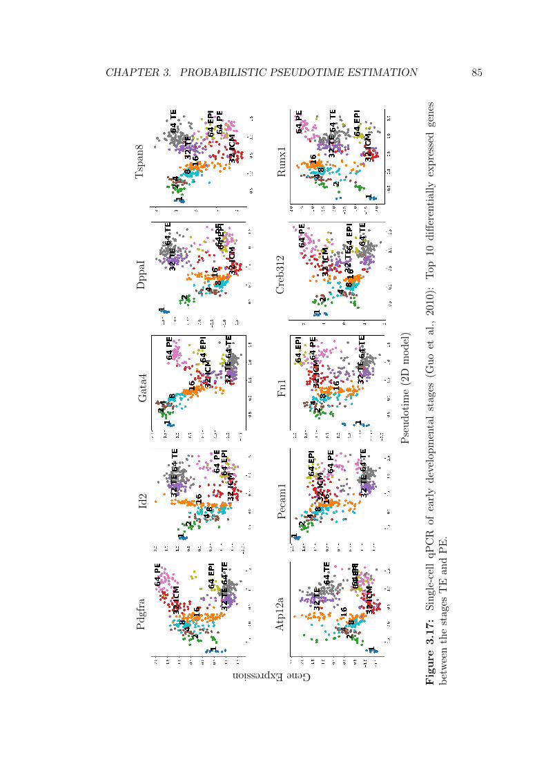
CHAPTER 3. PROBABILISTIC PSEUDOTIME ESTIMATION 85
Pdgf
raId
2G
ata4
DppaI
Tsp
an8
Atp
12a
Pec
am1
Fn1
Cre
b31
2R
unx1
GeneExpression
Pse
udot
ime
(2D
model
)
Fig
ure
3.1
7:
Sin
gle-
cell
qP
CR
ofea
rly
dev
elop
men
tal
stag
es(G
uo
etal
.,20
10):
Top
10diff
eren
tial
lyex
pre
ssed
genes
bet
wee
nth
est
ages
TE
and
PE
.

CHAPTER 3. PROBABILISTIC PSEUDOTIME ESTIMATION 86
Figure 3.18: Single-cell qPCR of early developmental stages (Guo et al., 2010):Heatmap showing the expression profiles of 48 genes across the pseudotime aswell as the added extra latent dimension.

CHAPTER 3. PROBABILISTIC PSEUDOTIME ESTIMATION 87
estimated pseudotime across a large range of prior variances. We also compare to
the case when no prior is used. We use two measures to assess model robustness:
rank correlation to the true experimental capture times (Figure 3.19 (a)) and rank
correlation to the estimated pseudotime using prior variance 0.1. In both figures,
the vertical black dashed line corresponds to the pseudotime at prior variance 0.1,
and the vertical red dashed line represents the model without a prior. The model
is sufficiently robust across the range of prior variances considered. As the prior
variance is increased, model performance gracefully deteriorates approaching the
performance achieved by the no-prior model.
3.3 Summary
Pseudotime estimation in single-cell genomics faces a number of challenges as
many sources of variability, both biological and technical, introduce a significant
amount of statistical uncertainty in the inference process. We develop a pseu-
dotime estimation method GrandPrix that uses a sparse variational Bayesian
GPLVM with an informative prior on the latent space.
Our model possesses several attractive features. Unlike other methods, it does
not require initial dimension reduction and so the mapping from latent variables
to genes is well defined. It is a probabilistic model, hence can provide not only
point estimation but also associated uncertainty which is useful for downstream
analysis (Campbell and Yau, 2016). It uses the VFE sparse approximation which
has an exact bound to the marginal likelihood and avoids overfitting unlike the
FITC approximation used by Reid and Wernisch (2016). Numerical calculations
can be carried out across different floating point precisions. The model is im-
plemented within the GPflow package and computation can be performed across
multiple CPU nodes and GPUs. Finally, the model can be extended to higher
dimensional latent spaces where the interaction of pseudotime with other factors
such as cell type differentiation, can be captured.
We evaluate the model by applying it on a number of datasets from different
organisms. The model produces similar results to the DeLorean model (Reid and
Wernisch, 2016), but typically converges faster. The model successfully repro-
duces the diffusion pseudotime (Haghverdi et al., 2016) for mouse embryonic stem
cells. The model’s scalability is tested by applying it on ∼68k peripheral blood
mononuclear cells, where the model converges quickly (∼6 mins). Finally, we

CHAPTER 3. PROBABILISTIC PSEUDOTIME ESTIMATION 88
Sp
earm
anco
rrel
atio
n
(a) Pseudotimes vs Capture time
Prior variance
Sp
earm
anco
rrel
atio
n
(b) Pseudotimes vs reported pseudotime
Prior variance
Figure 3.19: Single-cell qPCR of early developmental stages (Guo et al., 2010):Effect of changing the prior variance (horizontal axis) on the estimated pseudo-time. The vertical black dashed line represents the prior variance value 0.1 andthe vertical red dashed lines represent the no prior model. (a): Rank correlation(vertical axis) between the actual capture time and the estimated pseudotime.(b) Rank correlation (vertical axis) between the estimated pseudotime points andthe pseudotime using prior variance = 0.1. The model with informative prior ismore accurate even when using a large prior variance compared to the modelwithout a prior.

CHAPTER 3. PROBABILISTIC PSEUDOTIME ESTIMATION 89
have shown the additional flexibility of GrandPrix using a two dimensional latent
space where pseudotime is estimated jointly with the developmental branching
structure. We have also tested the model across mixed precision floating point
numbers, and using a lower precision offers further speed up.
In all cases, the model requires a small number of inducing points and less
computation to generate biologically plausible estimates compared to existing
approaches. Thus the scalability and flexibility of the proposed method ensures
its utility for analysing larger datasets such as those generated from droplet-based
techniques.
We have used i.i.d. Gaussian noise with uniform variance in our model. How-
ever, a non-uniform noise model may be a more suitable choice for single-cell
data as the variability of data points is a subject to change along the pseudo-
time trajectory or across genes. However, a non-uniform noise model requires
additional modelling of how the variability changes across pseudotime (Campbell
and Yau, 2016). Misspecification of the latter may lead to misleading conclusions
and we have therefore selected to use the simpler i.i.d. Gaussian noise with uni-
form variance in our approach. Similarly a count-based noise model may be a
more appropriate choice for single cell data. Using a non-Gaussian noise model
will make the model likelihood intractable and hence increase the computational
complexity of inference5.
Like other GP models, the GPLVM is also very susceptible to local minima.
From Figure 3.10, it is evident that the model converges to different local optima
for different number of inducing points as well as for different initialisations used.
To mitigate the effect of local minima we have used multiple restart using multiple
initial conditions, however it remains challenging to identify the global optimum
or suitable local optima in large-scale problems. Therefore, the GPLVM does
not currently provide an effective replacement for popular dimensionality reduc-
tion approaches such as tSNE or UMAP. However, with good prior information
available, the GPLVM can often find good latent representations.
5To learn more about sources of uncertainty in single-cell analysis, see Campbell and Yau(2016).

Chapter 4
Uncovering gene-specific
branching dynamics
To understand biological processes it is important to identify the events where
individual genes start to follow different lineages in the cellular trajectory readily
available from trajectory inference algorithms. Gaussian process (GP) provides a
flexible framework that can adequately accommodate the identification of gene-
specific branching dynamics.
We provide an efficient reimplementation of a method DEtime that was used
to identify perturbation time where two time courses start to differs. We have
applied this model in case of single-cell data to identify branching locations of
individual genes. We also address the limitations of the branching Gaussian
process (BGP) model, a downstream analysis tool for single-cell data, and extend
it to develop the multivariate BGP (mBGP) model. To scale up inference in
these applications we use sparse variational Bayesian inference algorithms to deal
with large matrix inversions and intractable likelihood functions. We examine
the effectiveness of our approaches on a synthetic dataset, a two sample time
course dataset and a single-cell RNA-seq dataset from mouse haematopoietic
stem cells (HSCs). Our approaches achieve similar levels of accuracy compared
to alternative studies while consistently maintaining biological plausibilities.
4.1 DEtime model
Yang et al. (2016) developed a Gaussian process based approach DEtime to iden-
tify the first point where two gene expression time-course profiles start to differ
90

CHAPTER 4. UNCOVERING GENE-SPECIFIC BRANCHING 91
from one another. They have termed this time point as perturbation time, later
referred to as bifurcation or branching time by Boukouvalas et al. (2018) with a
similar application in the case of single-cell data (see Section 4.3).
Let yc(T) and yp(T) represent noisy measurements of a control and a per-
turbed time course datasets respectively. Before the perturbation time tp, the two
time course profiles are considered as the noisy versions of the same underlying
mean function g(t),
yc(tn) = g(tn) + ε,
yp(tn) = g(tn) + ε for tn ≤ tp,(4.1)
where ε ∼ N (0, σ2noise) is the i.i.d.Gaussian noise with variance σ2
noise. After the
perturbation point tp, the mean function of the control data yc remains the same
and follows g(t) while the mean function of the perturbed data yp changes to
follow h(t),
yc(tn) = g(tn) + ε,
yp(tn) = h(tn) + ε for tn > tp .(4.2)
The idea is to define a joint covariance function k for the branching process
that imposes a constraint on two GP functions g and h to cross at a single point
tp. Now, placing Gaussian process priors on these two noise-free latent functions
and forcing them to intersect at tp, we have
g(t) ∼ GP (0, k (t, t′)) ,
h(t) ∼ GP (0, k (t, t′)) , (4.3)
g(tp) = h(tp) = u,
where k (t, t′) is the covariance function that imposes a smoothness constraint be-
tween two distinct time points t and t′; and u is the functional value at time point
tp. As u is unknown, it can be marginalised out using a Gaussian distribution
prior
u ∼ N (0, k(tp, tp)) ,
where k(tp, tp) is the covariance function evaluated at the intersection point only.

CHAPTER 4. UNCOVERING GENE-SPECIFIC BRANCHING 92
Thus the joint probability distribution of latent functions g and h is
p (g(T), h(T)) =
∫p(g|T, u)p(h|T, u)p(u)du
∝ exp
−1
2
(g
h
)T
Σ−1
(g
h
)∼ N (0,Σ) ,
(4.4)
where Σ is the covariance matrix having the following form
Σ =
(Kgg Kgh
Khg Khh
)=
(k(T,T) k(T,tp)k(T,tp)>
k(tp,tp)k(T,tp)k(T,tp)>
k(tp,tp)k(T,T)
), (4.5)
where k(T,T) and k(T, tp) are the covariance functions evaluated among all
training input time points T and between all training input time points T and
the intersection time point tp respectively. Figure 4.1(a) shows the example func-
tions (left sub-panel) as well as the structure of this covariance function (right
sub-panel). The input time points T are taken in the range [0, 100] and the in-
tersection point is set at tp = 50. Yang et al. (2016) have used this approach in
their study to investigate the changes a biological process undergoes after pertur-
bation. Their method uses datasets containing both perturbed and unperturbed
time courses, and provides a principled statistical approach that can identify a
specific time point at which two underlying time course data (perturbed and
unperturbed) start to differ after perturbation.
Since the latent functions g(t) and h(t) are constrained to intersect at the
perturbation time tp, they follow the Gaussian Process defined by the covariance
structure given in Equation (4.5). Thus, the joint probability distribution of yc
and yp conditioned on tp is,
p (yc(T), yp(T)|tp) ∝ exp
−1
2
(yc
yp
)>Σ−1
(yc
yp
) , (4.6)
∼ N(
0, Σ),
where Σ is the covariance matrix and can be figured out in terms of the covariance

CHAPTER 4. UNCOVERING GENE-SPECIFIC BRANCHING 93
(a)
(b)
Figure 4.1: Illustration of the covariance matrices proposed in Yang et al.(2016). The input T contains 100 evenly distributed time points within therange [0, 100] and the intersection or the perturbation time is set at tp = 50.(a): Two latent functions g and h are intersecting at the perturbation time tp(left sub-panel) and the covariance structure from which these two functions havebeen sampled (right sub-panel). The covariance matrix is evaluated at every pointwithin the input domain [0, 100] for both functions g and h. (b): The samplesand structure of resulting covariance matrix from a control and a perturbed timecourses yc and yp crossing at tp = 50. yc is evaluated at every time point withinthe range [0, 100], where yp is evaluated only the time points ≥ 50.

CHAPTER 4. UNCOVERING GENE-SPECIFIC BRANCHING 94
matrix Σ defined in Equation (4.5),
Σ =
(Kycyc Kycyp
Kypyc Kypyp
), (4.7)
with
Kyc(T1)yc(T2) = Kg(T1)g(T2) + σ2noiseI T1 ∈ T,T2 ∈ T
Kyc(T1)yp(T2) =
{Kg(T1)g(T2)
Kg(T1)h(T2)
T1 ∈ T,T2 ≤ tp
T1 ∈ T,T2 > tp
Kyp(T1)yc(T2) =
{Kg(T1)g(T2)
Kh(T1)g(T2)
T1 ≤ tp,T2 ∈ T
T1 > tp,T2 ∈ T
Kyp(T1)yp(T2) =
Kg(T1)g(T2) + σ2
noiseI
Kh(T1)g(T2)
Kg(T1)h(T2)
Kh(T1)h(T2) + σ2noiseI
T1 ≤ tp,T2 ≤ tp
T1 > tp,T2 ≤ tp
T2 > tp,T1 ≤ tp
T1 > tp,T2 > tp
Figure 4.1(b) shows an example of the covariance matrix Σ. The input time
points are taken evenly spread within the range [0, 100] with a perturbation time
point tp = 50.
4.1.1 Extension to non-Gaussian likelihood
Biological datasets are usually summarised as count data and the negative bi-
nomial (NB) distribution is considered a robust model for fitting counts data.
We have therefore implemented a NB likelihood to work with the GP regression
model. A negative binomial distribution is defined by a mean µ and a non-
negative dispersion parameter α. If y is the read count of a gene, the probability
mass function (PMF) is defined as,
y ∼ NB(µ, α)
=Γ(y + α)
y!Γ(α)
(α
α + µ
)α(µ
α + µ
)y, (4.8)
where Γ is the Gamma function.
A GP regression model with NB likelihood function needs to use a link func-
tion to relate the Gaussian process prior over the latent function f(t) to the

CHAPTER 4. UNCOVERING GENE-SPECIFIC BRANCHING 95
mean of the negative binomial distribution (see e.g. John and Hensman, 2018;
Aijo et al., 2014). We have used an exponential link function, therefore
µ = ef(t) .
The marginal likelihood of the model is,
p(y|T) =
∫p(y|f,T)︸ ︷︷ ︸
NB distribution
p(f |T, θ)df , (4.9)
where θ = {l, σ2} represents the kernel hyperparameters. Using negative binomial
as the likelihood function makes the GP model mathematically intractable. We
have used variational inference (see e.g. Bishop, 2006) to get an approximate
analytical solution of the model. Variational inference involves maximisation of
a variational lower bound
L(q, θ) , Eq(f) [log p(y|f, θ)]−DKL(q(f)||p(f |y)) (4.10)
where q(f) is the approximate posterior distribution. Traditionally, variational
inference algorithms use a tractable family of distribution as the proposal pos-
terior distribution (Opper and Archambeau, 2009; Tran et al., 2016). Here, we
have used the standard Gaussian distribution as the approximate posterior dis-
tribution q(f). Lower bound of Equation (4.10) has been maximised to learn
the model parameters, kernel hyperparameters as well as variational parameters.
The approximate marginal log-likelihood values calculated using Equation (4.10)
for different candidate perturbation points have been used to derive the posterior
distribution over the the perturbation point (see Section 4.1.2). We have also
adapted the sparse version of the variational inference (see Section 2.2.3) to make
the model computationally efficient for handling large datasets.
4.1.2 Inference
Yang et al. (2016) fitted their model using the standard Gaussian Process re-
gression approach described in Section 2.2.2. The perturbation time tp is a
hyperparameter of the joint covariance function of this model along with the
hyperparameters of the GP functions, i.e. lengthscale l and process variance σ2
. Yang et al. (2016) chose to estimate lengthscale and process variance prior to
inferring the perturbation time. The lengthscale and process variance can be

CHAPTER 4. UNCOVERING GENE-SPECIFIC BRANCHING 96
estimated reasonably by fitting two separate GP regression models to the data
from both control and perturbed conditions. The lengthscale and process vari-
ance hyper-parameters are shared across the data from two conditions and can
be estimated by maximum likelihood. To do so, Yang et al. (2016) have max-
imised the likelihood for the case where perturbation time tp approaches to −∞,
which corresponds to two independent GP regression models for the control and
perturbed time course data respectively,
θ = argmaxθ
(lim
tp→−∞pθ(y
c(T), yp(T)|tp, θ)), (4.11)
where θ = {l, σ2}. This leaves the problem of inferring the perturbation time tp
only. As this is a one-dimensional problem, the posterior distribution of tp can be
estimated by using a simple histogram approach. Yang et al. (2016) used a simple
discretisation tp ∈ [tmin, tmin + δ, tmin + 2δ, . . . , tmax] and estimated the posterior
by using the normalised likelihood evaluated at each grid point,
p(tp|yc(T), yp(T)) ' p(yc(T), yp(T)|tp)∑t=tmax
t=tminp(yc(T), yp(T)|t)
, (4.12)
which leverage the model to avoid the need of using complex optimisation or
integration schemes.
We have reimplemented the above approach within the GPflow package which
allows us further to adapt sparse approximation for Gaussian Process inference.
The flexible architecture of the GPflow package also allows the model to work
with non-Gaussian likelihood functions (see Section 4.2).
Figure 4.2 shows an example where we have applied this model on real time
course data that have been also used in Yang et al. (2016). To investigate the
biological significance of identifying gene-specific perturbation times, Yang et al.
(2016) applied their model on a two-sample gene expression time course data
from an experiment with Arabidopsis (Lewis et al., 2015). The experiment was
carried out by infecting the plant with a pathogen to produce the control time
series as well as infecting the plant with a mutated strain of the pathogen to
produce the perturbation time series. The resulting dataset captures changes
in gene expression profiles related to the development of defence and disease in
Arabidopsis.
Figure 4.2 (a) shows the expression profile of a gene with a perturbation

CHAPTER 4. UNCOVERING GENE-SPECIFIC BRANCHING 97
time point around the middle of the time course and Figure 4.2 (b) depicts the
expression profile of a gene with no perturbation. The posterior distribution of
the perturbation time is shown on the lower sub-panel in each case. When there
is no perturbation, the posterior distribution tends to increase towards the end
of the time range as shown in the lower sub-panel of Figure 4.2 (b).
The posterior probability returned by the model can be used to calculate the
Bayes factor that provides evidence for whether the two time courses diverge
(after any time) or are statistically indistinguishable. If the estimated perturba-
tion time is closer to the start of the time course, it is more likely that two time
courses are truly distinct. On the other hand, if the inferred perturbation time is
at the end of the time, it is very likely that the two samples are similar to each
other and are less likely to diverge. Thus a decision can be made over whether or
not there is a perturbation by considering the Bayes factor between a model with
or without a perturbation (Boukouvalas et al., 2018). The logged Bayes factor
between a model with or without perturbation is,
rg = logp(0 < tp < tmax|yc(T), yp(T))
p(tp = tmax|yc(T), yp(T))
= log
1
Nb
tp=tmax∑tp=tmin
p(yc(T), yp(T)|tp)
− log [p(yc(T), yp(T)|tmax)] ,(4.13)
where Nb is the number of bins in the histogram approximation to the posterior
and setting tp = tmax is equivalent to having no perturbation at all. Equa-
tion (4.13) assumes equal prior probability of having a perturbation (at any time
before tmax with equal probability) or not having a perturbation. If the height
of the posterior at the end of time is greater than the average of the posterior
over all earlier times as on the lower sub-panel of Figure 4.2 (b), the probability
of having a perturbation under the model is less than 0.5. As an example, the
evidence of having a perturbation is very strong in Figure 4.2 (a) with a logged
Bayes factor rg = 17.73 and there is fairly a strong evidence of having no pertur-
bation in Figure 4.2 (b) (rg = −3.33). This can be used to rank genes by how
likely it is that their expression profiles are diverging or differentially expressed.
Yang et al. (2016) and Boukouvalas et al. (2018) have used this approach to filter
differentially expressed genes from a large number of available genes prior to us-
ing their respective models for downstream analysis of identifying perturbation or
bifurcation time points. While larger logged Bayes factor indicative of stronger

CHAPTER 4. UNCOVERING GENE-SPECIFIC BRANCHING 98
evidence of branching, Boukouvalas et al. (2018) have found that most of the
branching genes have rg closer to zero thresholds. However, researchers can set
different cutoffs based on domain knowledge to filter genes, e.g. Yang et al. (2016)
have shown analysis using both rg > 4 and rg > 10. One appealing approach
can be calculating the logged Bayes factor for known marker genes and use these
values to determine cutoffs for filtering the desired number of genes (Boukouvalas
et al., 2018). A comprehensive study on the Bayes factor and its applications on
different scientific domains can be found in Kass and Raftery (1995).
Figure 4.3 shows an example where the model is applied on two genes from
the same two-sample gene expression dataset of Arabidopsis (Lewis et al., 2015).
The log normalised data were transformed to zero mean and unit standard de-
viation. Figure 4.3 (a) is an example of an early branching gene, while the gene
in Figure 4.3 (b) is an example of a late branching gene. In each case, the lower
sub-panel represents the posterior distribution over the perturbation time. Yang
et al. (2016) used this approach to rank genes according to perturbation times
from the earliest to the latest. They assigned genes to one of three groups: early,
intermediate and late perturbed genes, which facilitated understand the sequence
of events associated with the immune response to infection.
We have adapted the above-mentioned approach and have applied it on single-
cell RNA-seq to investigate genes that are differentially expressed between dif-
ferent cell lineages. Moreover, to deal with the inherent complexity of single-cell
data, along with the Gaussian likelihood we have also considered non-Gaussian
likelihoods in the GP regression model.
4.2 Identifying differentially expressed genes us-
ing single-cell data
Unlike time series, data from single-cell experiments lack actual time points and
the downstream analysis of identifying DE genes is carried out using pseudotem-
poral ordering of cells. Van den Berge et al. (2019) (Section 2.1.2) use the single-
cell RNA-seq of haematopoietic stem cells (HSCs) from mouse (Paul et al., 2015)
to benchmark the tradeSeq package. The data contain cells that are differenti-
ated into myeloid and erythroid precursor cell types. Paul et al. (2015) analysed
changes in gene expression for myeloid progenitors and created a reference com-
pendium of marker genes related to the development of erythrocytes and several
other types of leukocytes from myeloid progenitors.

CHAPTER 4. UNCOVERING GENE-SPECIFIC BRANCHING 99
Gen
eE
xp
ress
ion
Pro
bab
ilit
yof
per
turb
ati
on
Time
(a) PurturbationG
ene
Exp
ress
ion
Pro
bab
ilit
yof
per
turb
ati
on
Time
(b) No perturbationn
Figure 4.2: Arabidopsis thaliana time series (Lewis et al., 2015): two examplesof the Gaussian Process regression model fit based upon the maximum a posteri-ori (MAP) estimate of the perturbation time (upper sub-panels) and the posteriordistribution of the perturbation time conditioned on model hyperparameter eval-uated at tp = −1000 (lower sub-panels). (a): Gene CATMA1a00045 expressionprofile with a perturbation introduced around halfway along the time range. (b)Gene CATMA1a00180 expression profile without any perturbation. Without per-turbation, the posterior over the perturbation time tends to increase towards theend of the time range (lower sub-panel). A logged Bayes factor (Equation (4.13))(17.73 vs. −3.33) can be used to determine whether a gene expression is showingevidence of perturbation.

CHAPTER 4. UNCOVERING GENE-SPECIFIC BRANCHING 100
Gen
eE
xp
ress
ion
Pro
bab
ilit
yof
per
turb
ati
on
Time
(a) Early perturbationnG
ene
Exp
ress
ion
Pro
bab
ilit
yof
per
turb
ati
on
Time
(b) Late perturbationn
Figure 4.3: Arabidopsis thaliana time series (Lewis et al., 2015): perturba-tion time inference for a two-sample gene expression dataset. Arabidopsis geneexpression dynamics was studied after infection by a wild-type pathogen (bluepoints) and compared with infection by a mutated pathogen (red points). TheGP regression model fit based on the MAP estimate of the perturbation time(upper sub-panels) and the posterior distribution of the perturbation time (lowersub-panels). (a): An example of an early DE gene CATMA1a00010 and (b): anexample of a late DE gene CATMA1a00060 from A. thaliana time series data.

CHAPTER 4. UNCOVERING GENE-SPECIFIC BRANCHING 101
In their study, Van den Berge et al. (2019) have mentioned two small outlier
cell clusters related to the dendritic and eosinophyl cell types. These two outlier
cell clusters do not belong to any particular lineage and have been excluded from
trajectory inference and downstream analysis, which leaves 2660 cells under con-
sideration. For this experiment, tradeSeq downloads normalised data from Mono-
cle 3 vignette (http://cole-trapnell-lab.github.io/monocle-release/monocle3).
The data were normalised using size factors of individual cells and dispersion func-
tion of each gene. TradeSeq uses Slingshot to get trajectory-specific pseudotimes
as well as assignment of cells to different branches. UMAP (McInnes et al., 2018)
is used for initial dimension reduction for Slingshot. Since Slingshot requires cell
or cluster type information, Van den Berge et al. (2019) have clustered the data
using k-means (Lloyd, 1982) clustering algorithm with 7 clusters. As progenitor
cells are known, this information is fed into Slingshot to define the starting point
of the trajectories. Slingshot infers two lineages for this dataset. We have derived
Slingshot produced lineage-specific cell assignments as well as pseudotimes from
the tradeSeq vignette (statomics.github.io/tradeSeq) and have used them in
our investigation of genes that are differentially expressed between lineages. By
using the method introduced in Section 4.1 we can identify DE genes, similar to
tradeSeq, but we are also able to infer when (in pseudotime) each gene begins to
diverge.
Figure 4.4 shows an example where we have applied the DEtime model on the
mouse hematopoiesis single-cell RNA-seq data. The data were log normalised
and transformed to zero mean and unit standard deviation. Figure 4.4 (a) shows
an early branching gene (MPO) and Figure 4.4 (b) is an example of a late branch-
ing gene (LY6E). The upper sub-panels of Figure 4.4 show the Gaussian process
regression model fit with associated credible regions. Here, we have sub-sampled
the data and larger markers in Figure 4.4 represent the cells used in the inference
process. In each case, the bottom sup-panel depicts the posterior probability dis-
tribution over branching time, which reflects the significant amount of uncertainty
associated with the identification of precise branching time.
Figure 4.5 shows an example of the DEtime model with NB likelihood ap-
plied on the expression profiles of the same two genes used in Figure 4.41. The
normalised count data (downloaded from tradeSeq vignette) have been used for
1For NB likelihood figures, we have used lowess to smooth the percentiles through pseudo-time.

CHAPTER 4. UNCOVERING GENE-SPECIFIC BRANCHING 102
log
(Gen
eE
xp
ress
ion
+1)
Bra
nch
ing
pro
bab
ilit
y
Pseudotime
(a) Early branching
log
(Gen
eE
xp
ress
ion
+1)
Bra
nch
ing
pro
bab
ilit
y
Pseudotime
(b) Late branching
Figure 4.4: Mouse haematopoietic stem cells (Paul et al., 2015): two examplesof the DEtime with Gaussian likelihood model fit on the single-cell data. Cellsassignment to different branches as well as the pseudotime of each cell are calcu-lated using the Slingshot algorithm. In both cases, the upper sub-panel shows theGP regression fit based on the MAP estimate of the gene-specific differentiatingtime and the lower sub-panel shows the posterior distribution over the differenti-ating or branching time point. The bigger markers used in the upper sub-panelsto represent the sub-sampled cells that have been used in the inference. (a): Anexample of an early DE gene MPO and (b): an example of a late DE gene LY6E.

CHAPTER 4. UNCOVERING GENE-SPECIFIC BRANCHING 103
NB likelihood. In each case, the upper sub-panel shows the GP regression with
NB likelihood model fit with associated credible regions and the lower sub-panel
plots the posterior uncertainty of the branching location.
From Figure 4.4 and 4.5, it is evident that both models (DEtime with Gaus-
sian likelihood and DEtime with NB likelihood) can efficiently identify early and
late differentially expressed genes. Both of these models provide reasonably sim-
ilar MAP estimate as well as posterior probability of the branching time. As
single-cell data contain a lot of zeros, therefore when we look at the predictive
distribution of the data we find that the model with NB likelihood better models
the data. The credible regions are wide in the case of Gaussian likelihood and
still miss some points that have zero values. On the other hand, in the case of
NB likelihood the credible regions can adequately model the points having zero
values. However, a systematic comparison between these two approaches requires
to apply them on a large number of genes (both synthetic and real) having dif-
ferent kind of expression patterns with varying level of noise. In this thesis, our
interest is to quantify gene-specific branching locations for DE genes. Therefore,
we have applied these approaches only on known DE genes to highlight that both
approaches can identify gene-specific branching locations with a similar level of
accuracy for know biomarkers.
Paul et al. (2015) generated a list of biomarker genes for developing myeloid
cells in their extensive analysis. The top six genes from their list are PRTN3,
MPO, CAR2, CTSG, ELANE, and CAR1. They labelled all of these six genes
as the “key genes” of hematopoiesis process. Thus these six genes are signifi-
cantly differentially expressed between lineages. In fact it was found that MPO
and CAR2 differentiated between erythroid progenitors and myeloid progenitors,
where PRTN3 was identified as monocyte-specific, and the cluster of three genes
ELANE, PRTN3 and MPO was found as the strongest markers for myeloid pro-
genitors as well as monocytes (Van den Berge et al., 2019). We have used the
DEtime model to investigate the branching dynamics of these six marker genes.
Figure 4.6 and 4.7 show the examples of GP regression with Gaussian likeli-
hood and NB likelihood models applied on the six biomarkers respectively. Both
models can adequately accommodate the identification of genes having different
expression patterns between lineages.
Next, we investigate the robustness of this approach in identifying branching
locations for the genes that are differentially expressed across the lineages, but

CHAPTER 4. UNCOVERING GENE-SPECIFIC BRANCHING 104
Gen
eE
xp
ress
ion
(cou
nt)
Bra
nch
ing
pro
bab
ilit
y
Pseudotime
(a) Early branching
Gen
eE
xp
ress
ion
(cou
nt)
Bra
nch
ing
pro
bab
ilit
y
Pseudotime
(b) Late branching
Figure 4.5: Mouse haematopoietic stem cells (Paul et al., 2015): Mousehaematopoietic stem cells (Paul et al., 2015): two examples of the DEtime withNegative Binomial likelihood model fit on the single-cell data. Cells assignmentto different branches as well as the pseudotime of each cell are calculated usingthe Slingshot algorithm. In both cases, the upper sub-panel shows the GP re-gression fit based on the MAP estimate of the gene-specific differentiating timeand the lower sub-panel shows the posterior distribution over the differentiatingor branching time point. The bigger markers used in the upper sub-panels torepresent the sub-sampled cells that have been used in the inference. (a): Anexample of an early DE gene MPO and (b): an example of a late DE gene LY6E.

CHAPTER 4. UNCOVERING GENE-SPECIFIC BRANCHING 105
(a) MPO (b) PRTN3
(c) CTSG (d) CAR2
(e) ELANE (f) CAR1
Pseudotime
Figure 4.6: Mouse haematopoietic stem cells (Paul et al., 2015): Examples ofthe DEtime with Gaussian likelihood model fit on the top six biomarker genesfor developing myeloid cells. Cell assignment to different branches as well as thepseudotime of each cell are calculated using the Slingshot algorithm. The biggermarkers shown in all figures represent the sub-sampled cells that have been usedin the inference. The GP regression fit depicted is based on the MAP estimateof the gene-specific differentiating or branching time.

CHAPTER 4. UNCOVERING GENE-SPECIFIC BRANCHING 106
(a) MPO (b) PRTN3
(c) CTSG (d) CAR2
(e) ELANE (f) CAR1
Pseudotime
Figure 4.7: Mouse haematopoietic stem cells (Paul et al., 2015): Examples ofthe DEtime with Negative Binomial likelihood model fit on the top six biomarkergenes for developing myeloid cells. Cell assignment to different branches as wellas the pseudotime of each cell are calculated using the Slingshot algorithm. Thebigger markers shown in all figures represent the sub-sampled cells that havebeen used in the inference. The GP regression fit depicted is based on the MAPestimate of the gene-specific differentiating or branching time.

CHAPTER 4. UNCOVERING GENE-SPECIFIC BRANCHING 107
show very little or no evidence of having different expression patterns at the end.
TradeSeq denotes the top five genes having this type of expression patterns IRF8,
APOE, ERP29, PSAP, and LAMP1. All of these five genes are known regulators
of hematopoiesis and are discussed in previous studies (Shin et al., 2011; Kuro-
taki et al., 2014; Paul et al., 2015; Marquis et al., 2011; Murphy et al., 2011).
Identifying branching points for these genes is challenging as the model may be
deceived easily, which may lead to wrong inference of branching locations. Fig-
ure 4.8 shows the model with Gaussian likelihood and NB likelihood applied on
the expression profile of gene IRF8. In each case, the upper sub-panel shows the
GP regression model fit where the most probable branching location is identified
using the MAP estimate; and the lower sub-panel describes the posterior proba-
bility over branching location. From Figure 4.8 it is evident that both models can
identify gene-specific branching dynamics even when the gene expression patterns
are very similar.
Figure 4.9 and 4.10 show another two examples of genes APOE and ERP29
respectively. The posterior probability of the branching time for gene ERP29 in
Figure 4.10 indicates an interesting feature. The flat posterior distribution at the
end of time range suggests there is not strong evidence that the gene is branching.
To investigate that we have calculated the logged Bayes factor rg. We found rg =
−0.75 for the model with Gaussian likelihood (Figure 4.10 (a)) and rg = −1.04 for
the model with NB likelihood (Figure 4.10 (b)). Thus in both cases, the logged
Bayes factor also suggests a non differentiating scenario. The gene ERP29 is a
well known regulator of hematopoiesis, but the data we have are not reflecting
branching behaviour, still the model can identify the branching dynamics of this
gene. Thus the model’s efficiency of identifying DE genes relevant to biological
plausibilities spreads out a number of different kinds of expression patterns. While
both the models with Gaussian likelihood and NB likelihood give similar results
in terms of inferring divergence times, the Gaussian likelihood is more readily
extended to more complex models as inference is more straightforward (see e.g.
Section 4.3).
Although this approach is useful to analyse DE genes, uncovering branch-
ing dynamics for individual genes from single-cell data demands some additional
challenges to be addressed. Gene expression encompasses a high level of noise at
the single-cell level, therefore uncertainty regarding which cell belongs to which
branch needs to be considered with care. Boukouvalas et al. (2018) have developed

CHAPTER 4. UNCOVERING GENE-SPECIFIC BRANCHING 108
log
(Gen
eE
xp
ress
ion
+1)
Bra
nch
ing
pro
bab
ilit
y
Pseudotime
(a) Gaussian likelihood
Gen
eE
xp
ress
ion
(cou
nt)
Bra
nch
ing
pro
bab
ilit
y
Pseudotime
(b) Negative Binomial likelihood
Figure 4.8: Mouse haematopoietic stem cells (Paul et al., 2015): Examples ofthe DEtime model fit on gene IRF8 . This gene is differentially expressed butthe expression pattern does not show any evidence of DE at the end of timerange. Cell assignment to different branches as well as the pseudotime of eachcell are calculated using the Slingshot algorithm. In both cases, the upper sub-panel shows the GP regression fit based on the MAP estimate of the gene-specificdifferentiating time and the lower sub-panel shows the posterior distribution overthe differentiating or branching time point. The bigger markers used in the uppersub-panels to represent the sub-sampled cells that have been used in the inference.(a): Example of the model with Gaussian likelihood (b): example of the modelwith Negative Binomial likelihood.

CHAPTER 4. UNCOVERING GENE-SPECIFIC BRANCHING 109
log
(Gen
eE
xp
ress
ion
+1)
Bra
nch
ing
pro
bab
ilit
y
Pseudotime
(a) Gaussian likelihood
Gen
eE
xp
ress
ion
(cou
nt)
Bra
nch
ing
pro
bab
ilit
y
Pseudotime
(b) Negative Binomial likelihood
Figure 4.9: Mouse haematopoietic stem cells (Paul et al., 2015): Examples ofthe DEtime model fit on gene APOE. This gene is differentially expressed butthe expression pattern is showing very little evidence of DE at the end of timerange. Cell assignment to different branches as well as the pseudotime of eachcell are calculated using the Slingshot algorithm. In both cases, the upper sub-panel shows the GP regression fit based on the MAP estimate of the gene-specificdifferentiating time and the lower sub-panel shows the posterior distribution overthe differentiating or branching time point. The bigger markers used in the uppersub-panels to represent the sub-sampled cells that have been used in the inference.(a): Example of the model with Gaussian likelihood (b): example of the modelwith Negative Binomial likelihood.

CHAPTER 4. UNCOVERING GENE-SPECIFIC BRANCHING 110
log
(Gen
eE
xp
ress
ion
+1)
Bra
nch
ing
pro
bab
ilit
y
Pseudotime
(a) Gaussian likelihood
Gen
eE
xp
ress
ion
(cou
nt)
Bra
nch
ing
pro
bab
ilit
y
Pseudotime
(b) Negative Binomial likelihood
Figure 4.10: Mouse haematopoietic stem cells (Paul et al., 2015): Examplesof the DEtime model fit on gene ERP29. This gene is a well known regulatorof hematopoiesis but the expression pattern is showing very little evidence ofDE. Cell assignment to different branches as well as the pseudotime of each cellare calculated using the Slingshot algorithm. In both cases, the upper sub-panelshows the GP regression fit based on the MAP estimate of the gene-specificdifferentiating time and the lower sub-panel shows the posterior distribution overthe differentiating or branching time point. The bigger markers used in the uppersub-panels to represent the sub-sampled cells that have been used in the inference.(a): Example of the model with Gaussian likelihood (rg = −0.75) . (b): exampleof the model with Negative Binomial likelihood (rg = −1.04) .

CHAPTER 4. UNCOVERING GENE-SPECIFIC BRANCHING 111
a more general method branching Gaussian process (BGP) to infer gene-specific
branching dynamics, that provides a posterior estimate of branching locations for
each gene while taking into consideration the uncertainty regarding individual cell
assignment to different branches.
4.3 Branching Gaussian Process (BGP)
The Branching Gaussian Process (BGP) model (Boukouvalas et al., 2018) is de-
veloped on top of the DEtime method discussed in Section 4.1. Considering from
the single-cell data analysis perspectives, both of these models need pseudotime
to be known beforehand. But the model developed by Yang et al. (2016) also
needs all cells to be labelled with the branch each cell belongs to, whereas Boukou-
valas et al. (2018) developed BGP as a probabilistic model over global branching
structure and individual cells assignment to branches needs not be known be-
forehand. This allows BGP to estimate the posterior distribution of branching
time for each gene as well as to quantify uncertainty in assigning branch labels to
each cell. Quantifying this uncertainty is important specially for the genes that
branch earlier than the global branching point (as in Figure 4.12) as cells are
not assigned to a particular branch before the global branching point, hence cell
labels are unknown. The model may also be able to correct incorrect cell labels
from the trajectory inference stage.
BGP uses the Overlapping mixture of Gaussian Processes (OMGP) (Lazaro-
Gredilla et al., 2012) to probabilistically label cells with the branches they belong
to. The OMGP is a mixture model developed for time-series data where each
mixture component is a Gaussian Process function and a data point at any time
point can be assigned to any of the mixture component. For the single-cell data,
pseudotimes represent cells progression through development and are analogous
to time-series. Therefore, each pseudotime point or cell can be assigned to the
mixture components of OMGP similarly. However, in the standard OMGP, mix-
ture components are independent and are represented by individual latent GP
functions, but BGP wishes to model cellular trajectories that are branching.
Therefore, Boukouvalas et al. (2018) have generalised the OMGP model by intro-
ducing dependence among the mixture components. To do so, they have used an
extended version of the branching kernel (Section 4.3.1) which forces the latent
GP functions representing mixture components to intersect and hence to become

CHAPTER 4. UNCOVERING GENE-SPECIFIC BRANCHING 112
dependent on one another.
Thus, the BGP model introduces dependence among the mixture components
of the OMGP and uses similar branch structures to Yang et al. (2016). This gener-
alisation allowed the development of a probabilistic model over cellular branching
structure where cell assignment to different branches needs not to be computed
before hand. BGP allows the estimation of gene-specific branching location while
considering the associated uncertainty in the branch labels for individual cells.
4.3.1 Branching kernel
The branching kernel constrains the latent functions to cross at a branching point.
This is an extended version of the kernel designed in Yang et al. (2016). If the
trunk f and two branches g and h are constrained to intersect at the branching
time tg, then by placing the GP priors on all of these three functions we have,
f(t) ∼ GP (0, k (t, t′)) ,
g(t) ∼ GP (0, k (t, t′)) ,
h(t) ∼ GP (0, k (t, t′)) , (4.14)
f(tg) = g(tg) = h(tg) .
Although the same covariance function was used for all latent functions, the
extension to different covariance functions for different GP functions is quite
straightforward. It would allow the extensive applicability of the BGP model,
for example, one branch could be modelled as a periodic function and the other
branches as non-periodic. This additional flexibility would incur extra compu-
tational budget as more parameters needed to be trained (Boukouvalas et al.,
2018).
The resulting covariance matrix can be worked out in a similar fashion of
Equation (4.5)
Σ =
Kff Kfg Kfh
Kgf Kgg Kgh
Khf Khg Khh
, (4.15)
with
Kfg = K>gf , Kfh = K>hf , and Kgh = K>hg .

CHAPTER 4. UNCOVERING GENE-SPECIFIC BRANCHING 113
Unlike the DEtime model where two latent functions (one control and one
perturbed) were specified and only the control function spanned the branching
location, the BGP model considered three functions for a single branching point.
The BGP allows the discontinuity in the gradient among the trunk f and the two
branches g and h.
Figure 4.11 shows an example of the covariance structure used in Boukouvalas
et al. (2018). The input points are evenly distributed within the range [0, 10] and
the global branching point is tg = 4 . Figure 4.11 (a) shows the examples of func-
tions as well as covariance structure evaluated at every point in the input domain
[0, 10]. Figure 4.11 (b) shows the examples where the discontinuity between the
trunk state and two branches is considered. The trunk f is evaluated only before
the global branching point and two branches g and h are evaluated at every point
after the global branching point.
4.3.2 Inference
Let Y ∈ RN×1 be the expression profile of a gene in N cells and Mf is the
number of branches in global cellular trajectories. A set of dependent latent
Gaussian Process functions F = {f1, f2, . . . , fMf} following the covariance struc-
ture described in Section 4.3.1 can be used to represent the branches in a tree
which is analogous to the cellular trajectories with multiple branches. Each of
this latent function has been defined for each cell, and has size M × 1, where
M = NMf . This extended representation of the functions allows the model to
efficiently re-compute the marginal likelihood corresponds to different branching
locations (Boukouvalas et al., 2018). Let Z ∈ {0, 1}N×M be a binary indicator
matrix determining the assignment of N cells to one of the Mf branches or latent
functions where each row of Z can have only one non-zero entry. As Boukouvalas
et al. (2018) are considering probabilistic or soft assignment of individual cells to
different branches, the indicator matrix Z has to be inferred along with the set
of latent functions F . The model likelihood follows the standard OMGP,
p (Y |F,Z) = N(Y |ZF, σ2I
), (4.16)
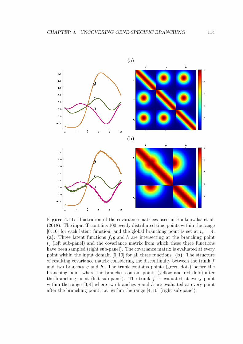
CHAPTER 4. UNCOVERING GENE-SPECIFIC BRANCHING 114
(a)
(b)
Figure 4.11: Illustration of the covariance matrices used in Boukouvalas et al.(2018). The input T contains 100 evenly distributed time points within the range[0, 10] for each latent function, and the global branching point is set at tg = 4.(a): Three latent functions f, g and h are intersecting at the branching pointtg (left sub-panel) and the covariance matrix from which these three functionshave been sampled (right sub-panel). The covariance matrix is evaluated at everypoint within the input domain [0, 10] for all three functions. (b): The structureof resulting covariance matrix considering the discontinuity between the trunk fand two branches g and h. The trunk contains points (green dots) before thebranching point where the branches contain points (yellow and red dots) afterthe branching point (left sub-panel). The trunk f is evaluated at every pointwithin the range [0, 4] where two branches g and h are evaluated at every pointafter the branching point, i.e. within the range [4, 10] (right sub-panel).

CHAPTER 4. UNCOVERING GENE-SPECIFIC BRANCHING 115
where σ2 is the noise variance and as in Lazaro-Gredilla et al. (2012) a categorical
prior was placed on the indicator matrix Z
p (Z) =N∏n=1
M∏m=1
[Π][Z]nmn,m , (4.17)
where for the multinomial distribution∑M
m=1 [Π]nm = 1 . As latent functions are
dependent in BGP, the GP priors over the latent functions do not factorise as the
standard OMGP. Boukouvalas et al. (2018) have placed the following GP prior
on the set of latent functions
p (F | tb) = GP (0, k|tb) , (4.18)
where k is the branching kernel (Section 4.3.1) that constrains the latent GP
functions to intersect at the gene-specific branching location tb.
The model’s hyperparameters can be estimated by maximising a bound on
the log likelihood. The log likelihood of the model is not analytically tractable as
it needs to integrate out the indicator matrix Z. Boukouvalas et al. (2018) have
used variational inference to derive an analytical solution for the lower bound as in
Lazaro-Gredilla et al. (2012), which involves the following mean-field assumption
q(Z, F ) = q(Z)q(F ) ,
where the latent functions F are considered independent of the indicator ma-
trix Z . A lower bound is derived using Jensen’s inequality (see e.g. King and
Lawrence, 2006)
log p (Y |F ) ≥ Eq(Z) [log p (Y |F,Z)]−DKL [q (Z) ||p (Z)] , (4.19)
where q (Z) =∏
n,m ΦZn,mn,m is the variational approximate distribution over Z
which encodes the mean-field assumption of the factorised posterior distribution
over the indicator matrix Z where Φn,m represents the posterior probability of
cell n assigning to branch m. The branch can be either the trunk state or one of
the branches. Next, F is integrated out to derive an exact variational collapsed
bound of the marginal log likelihood log p(Y ) (Boukouvalas et al., 2018).
The branching time posterior probability is calculated for one gene at a time
like the DEtime model. The approximate marginal log likelihood is calculated at
CHAPTER 4. UNCOVERING GENE-SPECIFIC BRANCHING 116
a set of candidate pseudotime points, and similar histogram approach of Equa-
tion (4.12) is used to derive the posterior distribution over the gene-specific
branching location. Boukouvalas et al. (2018) have also derived a sparse ap-
proximation bound of their model that allows BGP to scale up to continuously
growing larger single-cell datasets.
4.3.3 BGP results
The BGP requires pseudotime of each cell to be computed before the model is
applied. It also allows incorporation of some prior information about each gene’s
branching dynamics. By applying a pseudotime and global branching algorithm
such as the diffusion pseudotime (DPT) (Haghverdi et al., 2016), Monocle 2 (Qiu
et al., 2016), Wishbone (Setty et al., 2016), or Slingshot (Street et al., 2018),
the global branching pattern of the cells can be inferred. Consider that tg is
the global branching point in pseudotime but that genes may branch before or
after that point, or possibly not exhibit any branching. Let tb is the pseudotime
of branching, which is considered to be specific to a particular gene. If tb < tg
then the global branching provides no information about which branch the cell
belongs to for tb < t < tg . If tb > tg then the inferred global branching can be
used to increase the probability of a cell being assigned to a particular branch.
Boukouvalas et al. (2018) have used this approach to identify whether individual
gene expression is showing branching dynamics and whether the branching is
early or late in pseudotime. They have used the global branching pattern as an
informative prior p(Z) for all genes.
Figure 4.12 shows an example of the BGP model applied on an early branch-
ing gene from the mouse hematopoietic stem cells (Paul et al., 2015). The data
contain 4423 cells. The log normalised data were transformed to zero mean for
each individual gene. The DDRTree algorithm from Monocle 2 (Qiu et al., 2016)
is used to infer the global cellular branching pattern as well as pseudotime for
each cell. We have used a sub-sample of 870 cells and 30 inducing points to speed
up the model inference. Figure 4.12 (a) shows the prior cell assignment of all
4423 cells which has been derived by running the Monocle 2 algorithm. This
global branching structure is used as the informative prior. Figure 4.12 (b) shows
the posterior cell assignment of 870 cells that have been used in the inference
(top sub-panel). The cells that are away from the global branching time (the
black dashed line in Figure 4.12 (a)) have been assigned to either of the branches

CHAPTER 4. UNCOVERING GENE-SPECIFIC BRANCHING 117
with high confidence. On the other hand, the cells closer to or around the global
branching point possess high level of uncertainty. This is also the case for the
cells equidistant from both branches. The bottom sub-panel of Figure 4.12 (b)
shows the inferred gene-specific branching dynamics along with the posterior
probability of the branching location. This uncertainty has been also reflected
in Figure 4.12 (a) where the magenta background depicts the uncertainty asso-
ciated with the gene-specific branching time (the blue solid line). The uncertain
regions shown in both figures (magenta background in Figure 4.12 (a) and green
dots near branching-time in Figure 4.12 (b)) are indicative of how cell assign-
ment uncertainty is incorporated into the gene-specific branching-time posterior
uncertainty. It emphasises one of the major benefits of developing probabilistic
methods like the BGP for downstream analysis. As single-cell data are noisy, the
cell assignment to different branches should be probabilistic while identifying the
gene-specific branching dynamics.
While the BGP can identify gene specific branching times reliably and its
robustness is verified by comparing with the relevant methods, i.e. the Branch
Expression Analysis Modelling (BEAM) (Qiu et al., 2017b) and the Mixture of
Factor Analysers (MFA) (Campbell and Yau, 2017), the applicability of the BGP
is greatly hindered by its limitations and in some cases it seems impractical from
the biological point of view.
4.3.4 Limitations of the BGP
In the BGP model, the inference is performed independently per gene. This has
two significant drawbacks, namely i) potentially inconsistent cell assignments;
and ii) extensive computational requirements, which have limited the adoption
of the BGP model in practice.
Potentially inconsistent cell assignments
The most notable limitation of the BGP model is its gene-specific branch assign-
ment. For instance, consider the example of the BGP fit on the marker gene
CTSG shown in Figure 4.13. Figure 4.13 (a) shows the prior assignment on the
sub-sampled 771 cells that have been used in the inference. The black dashed
line represents the global branching points, the blue solid line is the inferred

CHAPTER 4. UNCOVERING GENE-SPECIFIC BRANCHING 118
0.0 0.2 0.4 0.6 0.8 1.0
0
25
50
75
100
125
150
Gen
eE
xp
ress
ion
Pseudotime
(a) Prior cell assignment
0.0 0.2 0.4 0.6 0.8 1.00.00
0.25
0.0 0.2 0.4 0.6 0.8 1.0
Gen
eE
xp
ress
ion
Pseudotime
(b) Posterior cell assignment
Figure 4.12: Mouse haematopoietic stem cells (Paul et al., 2015): BranchingGP (BGP) fit for the early branching gene MPO. The DDRTree algorithm ofMonocle 2 is used to estimate the pseudotime point for each cell as well as theglobal branching pattern. (a): Monocle 2 global assignment of cells to the trunkstate (purple) and two branches (green and red). The black dashed line is theglobal branching time. The most probable gene branching time is shown by theblue solid line along with posterior uncertainty over the branching location (ma-genta background). (b): The top sub-panel shows the posterior cell assignmentuncertainty for the cells used in the inference. For easy demonstration, the cellassignment to one of the branches is depicted. The bottom sub-panel representsthe posterior probability distribution over the gene-specific branching location.

CHAPTER 4. UNCOVERING GENE-SPECIFIC BRANCHING 119
gene-specific branching time and the magenta background is the associated un-
certainty over gene-specific branching location. The global branching pattern is
derived by using the Monocle 2 algorithm. The cells at the end of both branches
are the terminal cell states and the posterior should assign these cells with high
confidence to the same branches as in the prior assignments. However, we find
from Figure 4.13 (b) that the posterior assigns some terminal cells (highlighted
by the small blue box) to the alternate branch. This result may be uninformative
and may be misleading as well. Thus, to avoid cell reassignment to the alternate
branches after the global branching point, Boukouvalas et al. (2018) have used
a very strong prior assignment probability of 0.99 in their analysis of single-cell
data. They argued that it would simplify the interpretation of the results, as cells
would no longer switch their branch label. However this reduces the benefit of
the model and still fails to mitigate the cell reassignment problem completely.
Figure 4.14 shows the example where we have conducted the same experiment
of Figure 4.13 using the same experimental setup except a strong prior assignment
probability of 0.99 is used this time. Despite of using a very strong prior assign-
ment probability, the posterior labels some cells (shown in the small blue boxes)
to alternate branches. Although the number of cells changing branch labels is
reduced, the problem is not solved completely. However, as we are dealing with
single-cell data and considering the richness of gene-specific behaviour in differ-
ent branches, as well as sparse measurements of single-cell, this kind of branch
reassignment errors should be widespread. Thus it may be the case that these
terminal cells have been mislabelled by the global branching algorithm, Monocle
2 in this case, and BGP is trying to correct these.
Moreover, The single gene model BGP suffers with potentially inconsistent
cell assignments for different genes; a cell may be assigned to branch A for one
gene and to branch B for another gene. Notably, when analysing pioneer genes
that branch before the global branching time identified by a global method such
as Monocle 2, no prior information on cell branch assignment prior to the global
branching time is available. The assignment of such a pioneer cell to a particular
branch is indicative that the cell is biased towards that particular branch. But it
is not possible to make such a statement based on a single gene. As for another
gene the same cell may be biased towards the alternate branch. Boukouvalas
et al. (2018) have tried to mitigate the risk of inconsistent cell assignments by
placing a strong global prior over the cell assignments, but the problem remains.

CHAPTER 4. UNCOVERING GENE-SPECIFIC BRANCHING 120
In Table 4.1, we have summarised the posterior cell assignments where the
BGP model is applied on the top six biomarkers of HSCs. To ensure the cell
assignment consistency we have used a very strong cell assignment prior proba-
bility of 0.99 . By using this strong cell assignment prior probability, we assume
that cells after the global branching point in pseudotime ordering will no longer
switch their branches. The inference was carried out using the same sub-sampled
771 cells and using the same experimental setup for all genes. In each case, the
sparse model with 30 inducing points is used. Table 4.1 depicts the posterior cell
assignments to the top branch with a very high confidence (0.80) for all six genes.
For each gene, different number of cells show a very strong evidence of being
assigned to the top branch. These cells may actually belong to the top branch or
they have become biased towards the top branch in case of that particular gene.
As different number of cells have been identified for each gene, it clearly indicates
the inconsistent cell assignment.
In Table 4.2, we summarises the cell assignment consistency achieved by BGP.
For each pair of genes, we identify the number of cells that belong to the same
branches in both genes. We then use the total number of cells used in the inference
(771) to calculate the percentage (%) of cell assignment consistency obtained.
Different values in Table 4.2 represent the inconsistency in cell assignment. Thus
the cell assignment reported by the BGP is not informative rather likely to be
misleading. It undoubtedly will produce erroneous, confusing and uninterpretable
results.
Table 4.1: Posterior cell assignment to the top branch by BGP for the top sixbiomarkers of hematopoietic stem cells (HSCs)
Gene name MPO CTSG PRTN3 ELANE CAR2 CAR1
# Cells assigned to the
top branch with high 470 486 508 498 489 525
confidence (≥ 0.80)
Extensive computational requirements
As the BGP estimates the branching time posterior by using the normalised
approximated likelihood calculated at a set of candidate branching points over
the pseudotime domain, the computational requirements are very high when

CHAPTER 4. UNCOVERING GENE-SPECIFIC BRANCHING 121
0.0 0.2 0.4 0.6 0.8 1.010
0
10
20
30
40
Gen
eE
xp
ress
ion
Pseudotime
(a) Prior cell assignment
10
0
10
20
30
40
0.0 0.2 0.4 0.6 0.8 1.00
1
0.0 0.2 0.4 0.6 0.8 1.0
Gen
eE
xp
ress
ion
Pseudotime
(b) Posterior cell assignment
Figure 4.13: Mouse haematopoietic stem cells (Paul et al., 2015): BranchingGP (BGP) fit on the early branching biomarker CTSG. The DDRTree algorithmof Monocle 2 is used to estimate the pseudotime point for each cell as well as theglobal branching pattern. A strong prior assignment probability of 0.80 is used.The cells shown inside the small blue boxes in both figure have changed theirbranch labels from the prior cell assignments to the posterior cell assignments.
0.0 0.2 0.4 0.6 0.8 1.010
0
10
20
30
40
Gen
eE
xp
ress
ion
Pseudotime
(a) Prior cell assignment
10
0
10
20
30
40
0.0 0.2 0.4 0.6 0.8 1.00.0
0.5
0.0 0.2 0.4 0.6 0.8 1.0
Gen
eE
xp
ress
ion
Pseudotime
(b) Posterior cell assignment
Figure 4.14: Mouse haematopoietic stem cells (Paul et al., 2015): BranchingGP (BGP) fit on the early branching biomarker CTSG. The DDRTree algorithmof Monocle 2 is used to estimate the pseudotime point for each cell as well as theglobal branching pattern. A very strong prior assignment probability of 0.99 isused. The cells shown inside the small blue boxes in both figure have changed theirbranch labels from the prior cell assignments to the posterior cell assignments.

CHAPTER 4. UNCOVERING GENE-SPECIFIC BRANCHING 122
Table 4.2: Percentage (%) of cell assignment consistency achieved by BGP foreach pair of the top six biomarkers of hematopoietic stem cells (HSCs)
CTSG PRTN3 ELANE CAR2 CAR1
MPO 94 92 91 91 88
CTSG 96 96 96 92
PRTN3 96 96 92
ELANE 97 93
CAR2 95
analysing many genes. Although the model inference can be done in parallel
(per gene), this still requires a very high computational resource overall. For
instance, an experiments involving hundreds of genes will take many days of clus-
ter time. Boukouvalas et al. (2018) also had to sub-sample the cells in order to
minimise the per-gene computational time, but the computational requirements
still remain very high. This exceptionally high computational load makes their
model impractical in many instances.
To address the limitations discussed above, we propose the multivariate branch-
ing Gaussian Process (mBGP) which performs the inference jointly on all genes
of interest, as the cell assignment only make sense when considering all the rele-
vant genes together. This approach solves the inconsistency issue as well as being
computationally tractable and simpler to use.
4.4 Multivariate BGP (mBGP)
The mBGP approach involves two independent but complementary main ideas:
using a different branching time parameter for each gene, and using a gradient
based optimisation to infer gene-specific branching time.
Multiple branching points, one for each output-gene
We have modified the branching kernel (Section 4.3.1) to hold a branching time
vector with a single scalar value for each output-gene. All output-genes are in-
dependent and the likelihood factorises across multiple outputs. Thus, we can
modify the likelihood calculation to perform the relevant per output calculation

CHAPTER 4. UNCOVERING GENE-SPECIFIC BRANCHING 123
separately for each output (Section 4.4.1). The likelihood calculation passes the
output-gene index explicitly to the branching kernel to get output-specific likeli-
hood. The hyperparameters of the embedded kernel are shared for all outputs.
Gradient search
We have modified the learning algorithm to do dynamic filtering of the posterior
probability of associator Φ = Eq(z)(Z) and the Kullback-Leibler divergence term
DKL based on the current value of branching point (Section 4.4.1). This has
allowed us to use gradients. As the value of the branching point is changed at
each optimisation step, the Φ and the DKL terms are dynamically filtered with
entries before the branching point assigned to the trunk branch.
Using gradient removes the need to do a grid search which would be imprac-
tical in the many output scenario since we have a combinatorial explosion of the
number of combinations. Rather than doing a grid search we have performed
multiple restarts to mitigate the effect of local minima.
4.4.1 Inference
The derivation of the mBGP model directly follows the derivation of the BGP
model (Section 4.3.2), thus the terminologies used here have similar meaning. As
the likelihood factorises for multiple independent outputs, the extension of the
single-output likelihood of Equation (4.16) to multiple independent outputs is
straightforward
p (Y|F , Z) =D∏d=1
N(Yd|ZFd, σ2I
), (4.20)
where D is the number of outputs or genes, Yd is the dth column of the gene
expression matrix Y = {Y1, ..., YD} and Fd denotes the dth column vector from
the set of latent GP functions F = {F1, ..., FD} .
Y ∈ RN×D
F ∈ RM×D
Yd ∈ RN×1
Fd ∈ RM×1
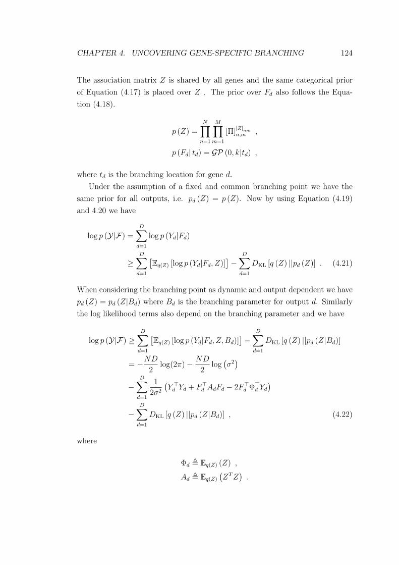
CHAPTER 4. UNCOVERING GENE-SPECIFIC BRANCHING 124
The association matrix Z is shared by all genes and the same categorical prior
of Equation (4.17) is placed over Z . The prior over Fd also follows the Equa-
tion (4.18).
p (Z) =N∏n=1
M∏m=1
[Π][Z]nmn,m ,
p (Fd| td) = GP (0, k|td) ,
where td is the branching location for gene d.
Under the assumption of a fixed and common branching point we have the
same prior for all outputs, i.e. pd (Z) = p (Z). Now by using Equation (4.19)
and 4.20 we have
log p (Y|F) =D∑d=1
log p (Yd|Fd)
≥D∑d=1
[Eq(Z) [log p (Yd|Fd, Z)]
]−
D∑d=1
DKL [q (Z) ||pd (Z)] . (4.21)
When considering the branching point as dynamic and output dependent we have
pd (Z) = pd (Z|Bd) where Bd is the branching parameter for output d. Similarly
the log likelihood terms also depend on the branching parameter and we have
log p (Y|F) ≥D∑d=1
[Eq(Z) [log p (Yd|Fd, Z,Bd)]
]−
D∑d=1
DKL [q (Z) ||pd (Z|Bd)]
= −ND2
log(2π)− ND
2log(σ2)
−D∑d=1
1
2σ2
(Y >d Yd + F>d AdFd − 2F>d Φ>d Yd
)−
D∑d=1
DKL [q (Z) ||pd (Z|Bd)] , (4.22)
where
Φd , Eq(Z) (Z) ,
Ad , Eq(Z)
(ZTZ
).

CHAPTER 4. UNCOVERING GENE-SPECIFIC BRANCHING 125
We have used the mean-field assumption as follows
q(Z,F) = q(Z)q(F) ,
where the variational approximate distribution over Z is similar to the original
BGP model,
q (Z) =∏n,m
ΦZn,mn,m ,
and q(F) factorises as
q(F) =D∏d=1
q(Fd) . (4.23)
Next we integrate out the latent GP functions F to derive the variational col-
lapsed bound for marginal log likelihood.
log p (Y) ≥− ND
2log(2πσ2)− 1
2σ2Y>Y − D
2
D∑d=1
log |Kffd|
− D
2
D∑d=1
log∣∣∣Adσ−2 +K−1
ffd
∣∣∣+D
2
D∑d=1
σ−4Y >d Φd
(Aσ−2 +K−1
ffd
)−1
Φ>d Yd
−D∑d=1
DKL [q (Z) ||pd (Z|Bd)] , (4.24)
where Kffd denotes the covariance matrix dependent on the output branching
parameter Bd. Finally, we have worked out the sparse variation lower bound for
our model.
Ls ,−ND
2log(2πσ2)− 1
2σ2YTY
− 1
2
D∑d=1
[log |Pd| − c>d cd
]− 1
2σ2
D∑d=1
[tr(AdKffd
)− tr
(AdKfudK
−1uudKufd
)]−
D∑d=1
DKL [q (Z) ||pd (Z|Bd)] , (4.25)

CHAPTER 4. UNCOVERING GENE-SPECIFIC BRANCHING 126
where
Pd , I + L−1d KufdAdKfudL
−>d σ−2 ,
Kuud , LdL>d ,
cd , R−1d L−1
d KufdΦ>d Ydσ−2 ,
Pd , RdR>d ,
u is the set of inducing points and subscript d is used to denote the dependence
on the branching time parameter Bd.
Unlike both the DEtime and the BGP models, our model considers all genes
at once. Thus, we cannot use the similar grid search or histogram approach as it
will give a combinatorial explosion of the number of possible combinations. Thus,
to infer gene-specific branching points, we have used gradient search.
Although it is possible to estimate lengthscale and process variance together
with the branching points, we prefer to estimate them prior to inferring branching
locations. We set the branching location of every gene at the starting of time (i.e.
Bd → 0) and estimate the lengthscale and the process variance hyperparameters
by maximum likelihood. After estimating lengthscale and process variance, there
remains branching points vector and associator (Z) to be inferred. We employ
multiple restart on the branching points while the associator is shared. By doing
gradient search we no longer have the posterior immediately available, however
we can estimate it using all the evaluations (for multiple restart) of the bound
evaluated by the optimiser.
4.4.2 Experimental results
Before applying our model, we need the pseudotime of each cell to be calculated.
If the global branching structure is available, we can incorporate it as an infor-
mative prior like the BGP model. We demonstrate the flexibility of our approach
by showing it can be used with different pseudotime methods for different case
studies. First we have applied our model on a synthetic dataset. The result
of this experiment motivates us to investigate the model’s applicability in real
single-cell domain. To demonstrate the effectiveness of our model on real data,
we have then applied it on single-cell RNA-seq data from mouse hematopoietic
stem cells (Paul et al., 2015).

CHAPTER 4. UNCOVERING GENE-SPECIFIC BRANCHING 127
Simulation study
The synthetic data are generated by using the branching GP model with a very
low noise. The data we used contains 75 cells and 8 genes. The data were log
normalised and transformed to zero mean. We have used the Monocle 2 algorithm
to obtain pseudotime of cells and global branching structure. We have used
the global branching structure as an informative prior with a prior assignment
probability of 0.80 . Among 8 genes, 2 genes branch early (tb = 0.1), 4 are
late (tb = 0.8) branching genes and 2 genes do not branch at all (tb = 1.1).
Figure 4.15 shows an example of the mBGP model fit on this data. In all sub-
figures the blue dotted lines are the actual branching times and the red dashed
lines are the estimated branching times. The model reasonably identifies gene-
specific branching times for all genes except an early branching gene (second one).
However, it is more useful to rank genes based on their branching times rather
than identifying the exact branching times, as in the case of real data we do not
know the actual branching time of any gene. Thus if we rank genes based on
the estimated branching times we see that we have the same rank as if we used
the actual branching times. In case of two “no branching” genes the estimated
branching times are shown at the end of the time range as we have truncated
them.
Synth
etic
Gen
eE
xp
ress
ion
Pseudotime
Figure 4.15: Simulation study: An example of the mBGP model fit on a syn-thetic dataset. The data contains early, late and no branching genes. The pseu-dotime is in interval [0, 1] . The blue dotted lines are the actual branching timesand the red dashed lines are the estimated branching time, which also depictedin the caption of of each sub-figure.

CHAPTER 4. UNCOVERING GENE-SPECIFIC BRANCHING 128
Hematopoiesis single-cell RNA-seq
We apply the mBGP model on the hematopoietic stem cells from mouse (Paul
et al., 2015), the same data used in the analysis of the BGP model and also
used by the tradeSeq authors. We have used the Wishbone algorithm (Setty
et al., 2016) to derive the pseudotime of each cell as well as the global branching
structure. This dataset was used in the original Wishbone analysis (Setty et al.,
2016) and we used Wishbone algorithm here to demonstrate the flexibility of our
model across different pseudotime methods. The model is also readily applicable
using pseudotime from other methods such as Monocle. The global branching
pattern is used as an informative prior where we have used prior assignment
probability 0.85 . Boukouvalas et al. (2018) have given a branching time network
of eight genes (Figure 4.16 (a)) that also includes the six biomarkers described
in Van den Berge et al. (2019). These eight genes show the highest evidence of
branching and have the logged Bayes factor rg ≥ 200 (Boukouvalas et al., 2018).
In the branching time network shown in Figure 4.16 (a), the most probable
branching time is annotated with each gene and directed edges are used to repre-
sent pairwise ordering of genes based on the most likely gene-specific branching
time. Boukouvalas et al. (2018) have grouped genes based on the branching time
order relationships among them. For instance, both PRTN3 and CTSG genes
belong to the same group (red group). These two genes are early branching genes
and branch before ELANE, GSTM1, CAR2 and CAR1. On the other hand,
MPO and CALR (yellow group) are also early branching genes and branch be-
fore GSTM1, CAR2 and CAR1, but not necessarily before ELANE. Finally, the
third group consists of genes ELANE and GSTM1 (blue group) that branch be-
fore the gene CAR1. The genes CAR2 and CAR2 can be considered the latest
branching time as there are no gene in this network branches after them.
We have applied the mBGP model on the expression profiles of these eight
genes. We have randomly sub-sampled the data and have used 443 cells for the
inference. We have used the sparse model with 60 inducing points. Figure 4.16 (b)
shows the mBGP model fit on this network of genes. In each sub-figure, the blue
dashed line represents the inferred gene-specific branching time, which is also
depicted inside the parenthesis of the sub-figure caption. Since the actual gene-
specific branching time is not defined for real data, we try to reproduce the same
pairwise ordering of genes already published in Boukouvalas et al. (2018). If we
compare the inferred gene-specific branching times from Figure 4.16 (b), we see

CHAPTER 4. UNCOVERING GENE-SPECIFIC BRANCHING 129
that our model has successfully reproduced the same branching time network of
Figure 4.16 (a). For instance, the inferred branching times for genes PRTN3
and CTSG (red group) are 0.12 and 0.9. These two genes branch earlier than
the genes ELANE (0.16), GSTM1 (0.30), CAR2 (0.28) and CAR1 (0.37), two
yellow group genes MPO (0.12) and CALR (0.17) branch before GSTM1 (0.30),
CAR2 (0.28) and CAR1 (0.37) and finally genes ELANE (0.16), GSTM1 (0.30)
(blue group) branch before CAR1 (0.37) as in the branching time network of
Figure 4.16 (a).
Next we include more genes in our inference. We include four marker genes
(APOE, GATA2, GATA1 and KLF1) for megakaryocyte erythroid progenitors
(MEPs). Figure 4.17 shows the mBGP model fit on the expression profiles of 12
biomarkers where have used prior assignment probability of 0.95. In each sub-
figure the blue dashed line corresponds to the inferred gene-specific branching
time which is also given inside the parenthesis of each sub-figure caption. If we
compare the branching times for individual genes, we see that they reproduce
the branching time network of Figure 4.16 (a). From Figure 4.17, it is evident
that the causal relationships between genes according to their branching times
are preserved and consistent with the network of Figure 4.16 (a). For instance,
red group genes PRTN3 (0.13) and CTSG (0.12) branch earlier than the genes
ELANE (0.16), GSTM1 (0.28), CAR2 (0.18) and CAR1 (0.35) as in the network
of Figure 4.16 (a). The same analogy can be derived for yellow and blue group
genes of Figure 4.16 (a) as well.
The inferred branching time for four other biomarkers (APOE, GATA2, GATA1
and KLF1) also reflect the biological plausibilities and consistent with the results
shown in Boukouvalas et al. (2018) (see Fig. 5c of Boukouvalas et al. (2018)). For
instance, we have already described in Section 4.2 that the expression profile of
the marker APOE shows transitory behaviour. It continues to increase after the
branching point, reaches its peak and then decreases to the level of the alternate
branch. Therefore, the expression profile of APOE shows very little evidence of
branching at the end of the time and the inference algorithm may fail to identify
the branching dynamics or may identify the branching location wrong. Boukou-
valas et al. (2018) have explained how the spline based approach BEAM (Qiu
et al., 2017b) incorrectly identifies the branching location. BEAM erroneously
identifies the last intersection point as the branching location (Boukouvalas et al.,
2018), but from Figure 4.17, we see that the mBGP model correctly identifies the

CHAPTER 4. UNCOVERING GENE-SPECIFIC BRANCHING 130
(a) Branching time gene networkG
ene
Exp
ress
ion
Pseudotime
(b) Estimated branching time
Figure 4.16: Mouse haematopoietic stem cells (Paul et al., 2015): (a): Branch-ing time network of genes showing very strong evidence of branching, loggedBayes factor rg > 200 (reuse with permission from Boukouvalas et al. (2018)).The most probable branching time of each gene is annotated. The directed edgesare used to represent the pairwise ordering of genes based on their branchingtime. The edge colours are representing group of genes having the same laterbranching genes. (b): The mBGP fit on the genes having the strongest evidenceof branching (rg > 200) . The cells (points) are coloured according to the globalbranching pattern derived using the Wishbone algorithm. The blue dashed linein each sub-figure represents the estimated branching time for each gene, whichis also depicted inside the parenthesis in each sub-figure caption.

CHAPTER 4. UNCOVERING GENE-SPECIFIC BRANCHING 131
branching time for the gene APOE. Thus the mBGP model is more robust against
a variety of gene expression patterns and can adequately identify the gene-specific
branching location that can explain the underlying biology.
Next we have analysed the posterior cell assignment by mBGP which follows
the global branching pattern provided as prior. As we have used a very strong
prior assignment probability (0.95), cells belonging to either branches do not
change branch label, i.e. both of the branches have the same cells in the prior
as well as in the posterior. Moreover, few cells from the trunk state become
biased towards either of the branches, which is also expected as they facilitate
the identification of pioneer genes. We have summarised this result in Table 4.3.
Gen
eE
xp
ress
ion
Pseudotime
Figure 4.17: Mouse haematopoietic stem cells (Paul et al., 2015): The mBGPfit on the expression profiles of 12 genes that show very strong evidence of branch-ing (Boukouvalas et al., 2018). The cells (points) are coloured according to theglobal branching pattern derived using the Wishbone algorithm. The blue dashedline in each sub-figure represents the estimated branching time for each gene,which is also depicted inside the parenthesis in each sub-figure caption.

CHAPTER 4. UNCOVERING GENE-SPECIFIC BRANCHING 132
Table 4.3: Comparison of prior and posterior cell assignment for the mBGPmodel
Number of cells
in prior in posterior change label to alternate branch
Branch 1 189 189 0
Branch 2 132 133 0
4.5 Summary
There are many ongoing challenges in analysing gene-specific branching dynamics
from single-cell data. Here we presented two approaches of identifying DE genes
as well as gene-specific branching locations. The models are developed within the
sparse variational Bayesian framework to facilitate the probabilistic downstream
analysis of extremely noisy single-cell data.
First, we reimplemented DEtime, a downstream analysis tool for bulk data.
We examine our implementation on the time series data used in Yang et al. (2016).
Then we extend this model to work with negative binomial (NB) likelihood and
applied it on single-cell mouse hematopoietic stem cell (HSC) data. The models
with Gaussian likelihood as well as NB likelihood adequately identify the bifurca-
tion points for the known marker genes even when the gene expression patterns
are very noisy.
Next, we discussed the BGP model followed by a detailed analysis of its lim-
itations, namely inconsistent cell assignments and heavy computational require-
ments. We develop the multivariate BGP (mBGP) model that extends BGP and
mitigates its limitations. We apply the model on a simulated data to verify its
effectiveness to identify gene-specific branching locations. Then we apply mBGP
on mouse hematopoietic stem cells. We use the expression patterns of the top
DE genes noted by Boukouvalas et al. (2018) where mBGP identifies branch-
ing time rank of genes similar to the BGP study while ensuring cell assignment
consistency.
It should be noted that if we consider the pairwise ordering of the top six
marker genes based on the branching times depicted in Figure 4.6, where Sling-
shot was used to pre-estimate pseudotime, we would derive a different branching

CHAPTER 4. UNCOVERING GENE-SPECIFIC BRANCHING 133
time network than Figure 4.16. In Section 2.3.1, we have discussed the associ-
ated uncertainty in pseudotime and trajectory estimation. Different pseudotime
algorithms generate different cell orderings and hence this uncertainty propagates
to downstream. Ideally, pseudotime uncertainty should also be included in the
model, although that model would be computationally challenging.
Although the proposed mBGP model infers a branching time network similar
to the BGP model, it does not learn cell assignment for the cells belonging to
the trunk state in this dataset. Table 4.3 shows that the cells before the global
branching points are not adequately biased towards any of the branches after
the inference. The reason may be the large number of parameters causing the
gradient search to be stuck at bad local minima. Using stochastic gradient descent
(SGD) may help the model to find better local minima. Moreover, a two-step
approach can be adopted for inference. After running the entire model, in the
second step, we can only use the genes that have a branching time closer to
the global branching point and cells that have a pseudotime before the global
branching time. The number of parameters will be reduced significantly in the
second step and the model may learn more meaningful cell to branch assignment
to facilitate the identification of branching locations for pioneer genes.

Chapter 5
Conclusion
In this thesis, we have presented scalable probabilistic methods for pseudotime
estimation and for post-processing to identify differentially expressed genes and
branching times. The models we presented are non-parametric in nature and
developed within the Bayesian framework. The core of our model is the Gaus-
sian process (GP) which has a long legacy in modelling data. As gene expression
is intrinsically noisy at single-cell resolution, GPs are a sensible choice as they
provide a means to capture model uncertainty, and incorporate prior knowledge.
However, the key bottleneck of applying GP models is that the full covariance
inversion (see Section 2.2.2), required at each iteration of hyperparameter opti-
misation, scales cubically, O(N3), where N is the number of cells in the case of
single-cell data. Therefore we developed our models using the sparse approxi-
mation technique that defines a small number of auxiliary or inducing variables,
that trade off fidelity to the full GP and computational speed. Specifically, for
M inducing points the inference scales as O(NM2) rather than O(N3), where
typically M � N (see Section 2.2.3).
Among a number of sparse approximation techniques, we have used the Vari-
ational Free Energy (VFE) approximation which provides an exact bound to the
marginal likelihood and avoids overfitting unlike other methods such as the FITC
approximation (see Section 2.2.3). Our models can use additional knowledge such
as cell capture times or cell labels to different branches as informative priors. Ex-
perimental results have shown how the incorporation of prior information helps
inference. Moreover, we have implemented our models within the GPflow pack-
age, a scalable software architecture that not only simplifies the implementation
due to the support for automatic differentiation but also allows lower precision
134

CHAPTER 5. CONCLUSION 135
and GPU computations for the necessary matrix operations.
Our approaches have been tested on a variety of datasets from different organ-
isms collected using different protocols. We find that our models have comparable
accuracy to alternative methods for inferring the posterior while converging con-
siderably faster.
5.1 Accomplished results
In Chapter 3, we presented GrandPrix. We have used the Bayesian GPLVM
model with informative priors to perform pseudotime estimation within a proba-
bilistic framework. The model uses cell capture times as priors over pseudotime.
Experimental results show that the properties of pseudotime ordering do not only
depend on the data but also on the prior assumptions about the trajectory such
as proximity to capture time, smoothness and periodicity.
The Bayesian GPLVM framework allows us to predict a number of latent
dimensions along with associated uncertainty. A sampling-based Markov Chain
Monte Carlo implementation of the Bayesian GPLVM is impractical for large
number of cells because of its high computational complexity. We have developed
our model on the basis of a sparse approximation that can generate a full posterior
using only a small number of inducing points.
Grandprix has been applied on a variety of datasets from different organ-
isms collected using different protocols. We find that Grandprix has comparable
accuracy to the DeLorean method for inferring the posterior mean pseudotime
across all datasets used in Reid and Wernisch (2016) while converging consider-
ably faster. The posterior mean from our model agrees closely with the posterior
mean from DeLorean in all cases, but we find that the posterior variance of both
the DeLorean and GrandPrix variational inference algorithms can be underes-
timated when compared to MCMC results (see Section 3.2.1). However, the
DeLorean approach does not scale to datasets with more than a few hundred
cells (Saelens et al., 2018). Our method therefore provides a practical approach
to incorporate prior information into pseudotime estimation but at the cost of
some loss in accuracy when assessing pseudotime uncertainties.
We have applied our model on droplet-based datasets to examine the robust-
ness and scalability of our approach on much larger datasets. Our model suc-
cessfully estimates pseudotimes for single-cell RNA-seq data of mouse embryonic
CHAPTER 5. CONCLUSION 136
stem cells (ESCs) generated using the inDrop protocol. The Bayesian GPLVM
estimated pseudotimes are in good agreement with DPT (Haghverdi et al., 2016)
whilst providing all the benefits of a fully probabilistic model; namely quantifi-
cation of uncertainty in the pseudotime estimation which has been shown to be
of biological relevance (Campbell and Yau, 2016). To demonstrate our models
scalability, we have measured its performance on a ∼68k single-cell dataset of
peripheral blood mononuclear cells. The model converges in 6 minutes on this
large dataset.
Finally, we have applied the model on single-cell qPCR of early developmental
stages to demonstrating its flexibility. We extended the model to higher dimen-
sional latent spaces where the interaction of pseudotime with other factors, such
as cell type differentiation, can be captured. We demonstrated the importance of
this additional flexibility using a two-dimensional latent space where pseudotime
is estimated jointly with the developmental branching structure.
The model performs well across varying floating point precisions. For droplet-
based datasets we have run the model using both 32 and 64 bit floating point
precision and the algorithm produces similar estimation of pseudotime. We expect
that in most cases, low precision will be sufficient to understand the behaviour of
the system offering a way to further scale up our approach without the need for
more expensive hardware. Mixed precision computations would also be possible
with higher-precision computations performed only on the most numerically crit-
ical parts of the algorithm maintaining high accuracy whilst being significantly
faster (Baboulin et al., 2009).
In Chapter 4, we presented two independent but complementary approaches
to inferring differentially expressed (DE) genes as well as gene-specific bifurcation
points.
First, we have reimplemented the downstream analysis tool DEtime (Yang
et al., 2016) for bulk data. The model was developed to detect the first point
(perturbation time) where two time series began to differ. This was done through
a novel covariance function for a branching process. We have extended the DE-
time model to work with both Gaussian likelihood and negative binomial (NB)
likelihood and have used it in downstream analysis of single-cell data.
We demonstrate the effectiveness of the model on a two-sample gene expres-
sion dataset from an experiment with Arabidopsis also used in Yang et al. (2016).
The model returns the posterior over the perturbation time, as well as providing

CHAPTER 5. CONCLUSION 137
evidence for whether the two time series differ (after any time) or are statisti-
cally indistinguishable. We then apply the model on single-cell RNA-seq from
mouse hematopoietic stem cells (HSCs). The model successfully infers the branch-
ing dynamics of biomarker genes for developing myeloid cells described by Paul
et al. (2015). The robustness of the model is examined on known regulators of
hematopoiesis where gene expression patterns are similar and show very little
evidence of differentially expressed.
In all the cases, we have examined the models with Gaussian likelihood and
NB likelihood. We find that both models can adequately identify DE expres-
sion patterns for known biomarkers similar to the tradeSeq package (Van den
Berge et al., 2019), but our models also provide posterior distributions over the
bifurcation times for individual genes.
Second, We briefly reviewed a single-cell downstream analysis tool, the branch-
ing Gaussian process (BGP), and provided a detailed analysis of the limitations
of this model. In BGP, inference is carried out for each gene separately which cre-
ates a potential threat of inconsistent cell assignment. Moreover, computational
requirements become very high when the model needs to analyse many genes.
We presented the multivariate branching Gaussian process (mBGP) model,
which is an extension of the BGP model and mitigates the limitations of the
latter. In mBGP, inference is performed for all genes of interest together where
cell assignment to different lineages is shared. mBGP avoids the danger of cell
assignment inconsistency and is computationally efficient as it employs gradient
search instead of grid search (see Section 4.4).
The mBGP model’s performance is evaluated on a simulated dataset where the
model infers branching dynamics for early, late and no-branching genes. We then
apply the model on the expression patterns of known biomarkers from single-cell
RNA-seq of mouse hematopoietic stem cells (HSCs). mBGP reproduces the same
branching time network of the marker genes showing highest evidence branching
published in Boukouvalas et al. (2018) (Figure 4.16). Experimental results also
demonstrate the robustness of mBGP in inferring gene-specific branching dynam-
ics across a variety of expression patterns even when they may show very little
or no evidence of branching towards the end of pseudotime (Figure 4.17).

CHAPTER 5. CONCLUSION 138
5.2 Research output
The work presented in this thesis contributed to a scientific publication, a book
chapter, an open-source software package and several conference presentations
(talks and posters).
Publication
Sumon Ahmed, Magnus Rattray, and Alexis Boukouvalas. Grandprix: scal-
ing up the bayesian gplvm for single-cell data. Bioinformatics, 35(1):47–54,
2018
Book chapter
Magnus Rattray, Jing Yang, Sumon Ahmed, and Alexis Boukouvalas. Mod-
elling gene expression dynamics with gaussian process inference. Handbook
of Statistical Genomics 4e 2V SET, pages 879–20, 2019
Software package
Python package: GrandPrix
Availability: github.com/ManchesterBioinference/GrandPrix.
Selected presentations
Poster Scaling up probabilistic pseudotime estimation with the GPLVM.
ISMB/ECCB,Prague, 2017 .
Full talk and Poster Using GrandPrix to investigate haematopoietic stem
cell development by single-cell sequencing. ISMB,Chicago, 2018 .
Full talk Uncovering gene-specific branching dynamics using multivariate
branching Gaussian process (mBGP). MASAMB,Cambridge, 2019 .
Poster Uncovering gene-specific branching dynamics using single-cell data.
ISMB,Prague, 2019 .

CHAPTER 5. CONCLUSION 139
5.3 Future work
Based on the achieved results discussed above, several promising avenues of fu-
ture work are immediate which involve addressing the limitations of the current
contributions as well as possible further extensions.
5.3.1 Pseudotime inference
In Section 3.2.6, we have shown that at the time of inferring pseudotime using
GPLVM, extra latent dimensions can be used to describe other biological func-
tions such as branching. The model can be extended to include additional prior
information on these extra latent dimensions; for example the prior could include
information on branching dynamics extracted from the application of branch-
ing models such as Monocle (Qiu et al., 2017b), DPT (Haghverdi et al., 2016),
Slingshot (Street et al., 2018) and Wishbone (Setty et al., 2016).
La Manno et al. (2018) used a kinetic model and predicted the changes of
mRNA expression levels in individual cells at single-cell resolution. They defined
RNA velocity as a high dimensional vector describing the time derivative of gene
expression state. From the definition it is evident that RNA velocity can predict
the future state of each cell in terms of changes in gene expression patterns
as well as the direction or lineages individual cells tend to follow. Gaussian
process models are readily extended to incorporate derivative information. As
differentiation is a linear operation, therefore the derivative of a Gaussian process
is also a Gaussian process (Rasmussen and Williams, 2006). It is possible to
extend the Bayesian GPLVM approach to make inferences based on RNA velocity
and to make predictions about cell fates. In general, the idea is to perform
inference based on a joint Gaussian distribution of function values (expression
profiles) and its time derivatives (RNA velocity). GPs provide a very flexible
architecture to achieve this, we just need to define a mixed covariance function on
function values, between function values and time derivatives, and between time
derivatives1. Such an extension could be useful for inferring complex trajectories
involving branching, cell cycle and oscillation. In these type of trajectories, gene
expressions may be similar at two different pseudotime or vice versa. Therefore
incorporation of time derivatives that reflect the changes in gene expression with
1To learn more about derivative observations Gaussian process, see Rasmussen and Williams(2006).

CHAPTER 5. CONCLUSION 140
respect to time, promises to facilitate the model in identifying more biologically
significant trajectories.
5.3.2 Branching inference
In our work at Chapter 4, we have considered a single branching point, but in
practice biological systems may contain multiple lineages. Although considerable
advances have been made in trajectory inference algorithms, the problem of accu-
rate characterisation of trajectories with multiple lineages remains unsolved. The
biggest challenge for these methods is determinig the number as well as the loca-
tions of bifurcation events. Some methods restrict the number of branches (e.g.
Setty et al., 2016) , whereas some methods need the user to specify the number
of branches (e.g. Trapnell et al., 2014) and there are also methods that use less
supervision while identifying lineages structure (e.g. Qiu et al., 2016; Street et al.,
2018). But there is no principled framework.
The branching covariance function we presented and used in Chapter 4 can be
easily extended for multiple branching points. Then by using Gaussian process
regression with the extended branching kernel it is possible to define a principled
framework to determine the number and the locations of branching points. To do
so, the pseudotime and global branching structure can be inferred using multiple
lineages trajectory inference algorithms such as Slingshot and Monocle 2. Let us
assume the global branching algorithm gives us C number of branching points.
We can define a set of extended branching kernels for the number of branching
points in {0, ..., C} , where the cells belong to the ignored branches (when number
of branching points is less than C) will be merged to other branches. Now we can
build separate GP regression model using each of these kernels and calculate the
marginal likelihood. In principle, if B is the number of branching points (0 ≤ B ≤C) that best describes the data, the GP regression model with branching kernel
having B branching points will have the maximum marginal likelihood. This is
a classical example of GP model selection and can readily be implemented by
extending the DEtime model described in Section 4.1.
The extended branching covariance function is also applicable with the BGP
and the mBGP model and may facilitate the identification of more complex gene-
specific branching dynamics. However, this approach requires the model to deal
with much harder optimisation challenges, since these models consider cell as-
signment uncertainty and re-estimate cell assignment to different branches as a
part of the inference process.

CHAPTER 5. CONCLUSION 141
5.3.3 Inferring pseudotime-branching
The mBGP method (BGP as well) we presented, infers gene-specific branching
after applying another algorithm for inferring pseudotime and the global cellular
branching. So far all existing methods of trajectory inference are two-step pro-
cedures. There are methods that first learn pseudotime of cells followed by the
inference of the global branching structure (e.g. Lonnberg et al., 2017). These
methods do assume that pseudotimes are known without error, when in reality
pseudotime inference is associated with high levels of uncertainty (Campbell and
Yau, 2016). On the other hand, there are methods that first learn the lineages
structure and then infer pseudotime of cells for individual lineages (e.g. Street
et al., 2018). These methods do not fully take into account errors and uncer-
tainty in this initial cell labelling stage prior to pseudotime inference (Boukou-
valas et al., 2018). An interesting extension would therefore be to combine the
mBGP and GPLVM models (an overlapping mixture of GPLVMs with branch-
ing kernel) to jointly model branching and infer latent manifolds from single-cell
expression data, taking all sources of error into account through use of a unified
model.
As a part of this project, we have already developed an open source software
package (e.g. GrandPrix) and a few others (e.g. mBGP) are going to be avail-
able soon. A significant portion of our future efforts involves maintaining these
packages. This includes improving the usability of the software, providing better
documentation and supporting other researchers in analysing their data using our
applications. It is also important to adequately accommodate future trends in
very rapidly growing single-cell sequencing.
Bibliography
Sumon Ahmed, Magnus Rattray, and Alexis Boukouvalas. Grandprix: scaling up
the bayesian gplvm for single-cell data. Bioinformatics, 35(1):47–54, 2018.
Tarmo Aijo, Vincent Butty, Zhi Chen, Verna Salo, Subhash Tripathi, Christo-
pher B Burge, Riitta Lahesmaa, and Harri Lahdesmaki. Methods for time
series analysis of rna-seq data with application to human th17 cell differentia-
tion. Bioinformatics, 30(12):i113–i120, 2014.
Simon Anders and Wolfgang Huber. Differential expression analysis for sequence
count data. Genome biology, 11(10):R106, 2010.
Marc Baboulin, Alfredo Buttari, Jack Dongarra, Jakub Kurzak, Julie Langou,
Julien Langou, Piotr Luszczek, and Stanimire Tomov. Accelerating scientific
computations with mixed precision algorithms. Computer Physics Communi-
cations, 180(12):2526–2533, 2009.
Matthias Bauer, Mark van der Wilk, and Carl Edward Rasmussen. Understanding
probabilistic sparse gaussian process approximations. In Advances in Neural
Information Processing Systems, pages 1533–1541, 2016.
Burkhard Becher, Andreas Schlitzer, Jinmiao Chen, Florian Mair, Hermi R Suma-
toh, Karen Wei Weng Teng, Donovan Low, Christiane Ruedl, Paola Riccardi-
Castagnoli, Michael Poidinger, et al. High-dimensional analysis of the murine
myeloid cell system. Nature immunology, 15(12):1181–1189, 2014.
Sean C Bendall, Kara L Davis, El-ad David Amir, Michelle D Tadmor, Erin F
Simonds, Tiffany J Chen, Daniel K Shenfeld, Garry P Nolan, and Dana Peer.
Single-cell trajectory detection uncovers progression and regulatory coordina-
tion in human b cell development. Cell, 157(3):714–725, 2014.
142

BIBLIOGRAPHY 143
Eli Bingham, Jonathan P Chen, Martin Jankowiak, Fritz Obermeyer, Neeraj
Pradhan, Theofanis Karaletsos, Rohit Singh, Paul Szerlip, Paul Horsfall, and
Noah D Goodman. Pyro: Deep universal probabilistic programming. The
Journal of Machine Learning Research, 20(1):973–978, 2019.
Christopher M Bishop. Pattern recognition and machine learning. springer, 2006.
David M Blei, Michael I Jordan, et al. Variational inference for dirichlet process
mixtures. Bayesian analysis, 1(1):121–143, 2006.
David M Blei, Alp Kucukelbir, and Jon D McAuliffe. Variational inference: A
review for statisticians. Journal of the American Statistical Association, 112
(518):859–877, 2017.
Vincent D Blondel, Jean-Loup Guillaume, Renaud Lambiotte, and Etienne Lefeb-
vre. Fast unfolding of communities in large networks. Journal of statistical
mechanics: theory and experiment, 2008(10):P10008, 2008.
Alexis Boukouvalas, James Hensman, and Magnus Rattray. BGP: identifying
gene-specific branching dynamics from single-cell data with a branching gaus-
sian process. Genome biology, 19(1):65, 2018.
Alexis Boukouvalas, Luisa Cutillo, Elli Marinopoulou, Nancy Papalopulu, and
Magnus Rattray. Osconet: Inferring oscillatory gene networks. bioRxiv, page
600049, 2019.
Michael Braun and Jon McAuliffe. Variational inference for large-scale models
of discrete choice. Journal of the American Statistical Association, 105(489):
324–335, 2010.
Elizabeth Buckingham-Jeffery, Valerie Isham, and Thomas House. Gaussian pro-
cess approximations for fast inference from infectious disease data. Mathemat-
ical biosciences, 301:111–120, 2018.
Florian Buettner and Fabian J Theis. A novel approach for resolving differences in
single-cell gene expression patterns from zygote to blastocyst. Bioinformatics,
28(18):i626–i632, 2012.
Florian Buettner, Kedar N Natarajan, F Paolo Casale, Valentina Proserpio, An-
tonio Scialdone, Fabian J Theis, Sarah A Teichmann, John C Marioni, and
BIBLIOGRAPHY 144
Oliver Stegle. Computational analysis of cell-to-cell heterogeneity in single-cell
rna-sequencing data reveals hidden subpopulations of cells. Nature biotechnol-
ogy, 33(2):155–160, 2015.
David Burt, Carl Edward Rasmussen, and Mark Van Der Wilk. Rates of con-
vergence for sparse variational gaussian process regression. In International
Conference on Machine Learning, pages 862–871, 2019.
Kieran Campbell and Christopher Yau. Order under uncertainty: robust differ-
ential expression analysis using probabilistic models for pseudotime inference.
PLoS Computational Biology, 12(11), 2016.
Kieran Campbell, Chris P Ponting, and Caleb Webber. Laplacian eigenmaps
and principal curves for high resolution pseudotemporal ordering of single-cell
rna-seq profiles. bioRxiv preprint, page 027219, 2015.
Kieran R Campbell and Christopher Yau. Probabilistic modeling of bifurcations
in single-cell gene expression data using a bayesian mixture of factor analyzers.
Wellcome open research, 2, 2017.
Junyue Cao, Malte Spielmann, Xiaojie Qiu, Xingfan Huang, Daniel M Ibrahim,
Andrew J Hill, Fan Zhang, Stefan Mundlos, Lena Christiansen, Frank J
Steemers, et al. The single-cell transcriptional landscape of mammalian organo-
genesis. Nature, 566(7745):496, 2019.
Edward Challis, Peter Hurley, Laura Serra, Marco Bozzali, Seb Oliver, and Mara
Cercignani. Gaussian process classification of alzheimer’s disease and mild
cognitive impairment from resting-state fmri. NeuroImage, 112:232–243, 2015.
Guokai Chen, Daniel R Gulbranson, Zhonggang Hou, Jennifer M Bolin, Victor
Ruotti, Mitchell D Probasco, Kimberly Smuga-Otto, Sara E Howden, Nicole R
Diol, Nicholas E Propson, et al. Chemically defined conditions for human ipsc
derivation and culture. Nature methods, 8(5):424, 2011.
Ronald R Coifman, Stephane Lafon, Ann B Lee, Mauro Maggioni, Boaz Nadler,
Frederick Warner, and Steven W Zucker. Geometric diffusions as a tool for
harmonic analysis and structure definition of data: Diffusion maps. Proceedings
of the national academy of sciences, 102(21):7426–7431, 2005.
BIBLIOGRAPHY 145
Zhenwen Dai, Andreas Damianou, James Hensman, and Neil Lawrence. Gaus-
sian process models with parallelization and gpu acceleration. arXiv preprint
arXiv:1410.4984, 2014.
Andreas C Damianou, Michalis K Titsias, and Neil D Lawrence. Variational
inference for latent variables and uncertain inputs in gaussian processes. The
Journal of Machine Learning Research, 17(1):1425–1486, 2016.
John T Dimos, Kit T Rodolfa, Kathy K Niakan, Laurin M Weisenthal, Hiroshi
Mitsumoto, Wendy Chung, Gist F Croft, Genevieve Saphier, Rudy Leibel,
Robin Goland, et al. Induced pluripotent stem cells generated from patients
with als can be differentiated into motor neurons. science, 321(5893):1218–
1221, 2008.
Alexander Dobin, Carrie A Davis, Felix Schlesinger, Jorg Drenkow, Chris Zaleski,
Sonali Jha, Philippe Batut, Mark Chaisson, and Thomas R Gingeras. Star:
ultrafast universal rna-seq aligner. Bioinformatics, 29(1):15–21, 2013.
David Duvenaud, James Robert Lloyd, Roger Grosse, Joshua B Tenenbaum, and
Zoubin Ghahramani. Structure discovery in nonparametric regression through
compositional kernel search. arXiv preprint arXiv:1302.4922, 2013.
Robert W Eyre, Thomas House, F Xavier Gomez-Olive, and Frances E Griffiths.
Modelling fertility in rural south africa with combined nonlinear parametric and
semi-parametric methods. Emerging themes in epidemiology, 15(1):5, 2018.
Russell B Fletcher, Diya Das, Levi Gadye, Kelly N Street, Ariane Baudhuin,
Allon Wagner, Michael B Cole, Quetzal Flores, Yoon Gi Choi, Nir Yosef, et al.
Deconstructing olfactory stem cell trajectories at single-cell resolution. Cell
stem cell, 20(6):817–830, 2017.
Tobias Galla. Intrinsic fluctuations in stochastic delay systems: Theoretical de-
scription and application to a simple model of gene regulation. Physical Review
E, 80(2):021909, 2009.
Jacob Gardner, Geoff Pleiss, Kilian Q Weinberger, David Bindel, and Andrew G
Wilson. Gpytorch: Blackbox matrix-matrix gaussian process inference with
gpu acceleration. In Advances in Neural Information Processing Systems, pages
7576–7586, 2018.

BIBLIOGRAPHY 146
Charles Gawad, Winston Koh, and Stephen R Quake. Single-cell genome se-
quencing: current state of the science. Nature Reviews Genetics, 17(3):175,
2016.
Alexander N Gorban and Andrei Y Zinovyev. Principal graphs and manifolds. In
Handbook of research on machine learning applications and trends: algorithms,
methods, and techniques, pages 28–59. IGI Global, 2010.
GPy. GPy: A gaussian process framework in python, since 2012.
Dominic Grun, Anna Lyubimova, Lennart Kester, Kay Wiebrands, Onur Basak,
Nobuo Sasaki, Hans Clevers, and Alexander van Oudenaarden. Single-cell
messenger rna sequencing reveals rare intestinal cell types. Nature, 525(7568):
251, 2015.
Guoji Guo, Mikael Huss, Guo Qing Tong, Chaoyang Wang, Li Li Sun, Neil D
Clarke, and Paul Robson. Resolution of cell fate decisions revealed by single-
cell gene expression analysis from zygote to blastocyst. Developmental cell, 18
(4):675–685, 2010.
Laleh Haghverdi, Florian Buettner, and Fabian J Theis. Diffusion maps for high-
dimensional single-cell analysis of differentiation data. Bioinformatics, 31(18):
2989–2998, 2015.
Laleh Haghverdi, Maren Buettner, F Alexander Wolf, Florian Buettner, and
Fabian J Theis. Diffusion pseudotime robustly reconstructs lineage branch-
ing. Nature methods, 13(10):845, 2016.
Trevor Hastie and Werner Stuetzle. Principal curves. Journal of the American
Statistical Association, 84(406):502–516, 1989.
Markus Heinonen, Olivier Guipaud, Fabien Milliat, Valerie Buard, Beatrice
Micheau, Georges Tarlet, Marc Benderitter, Farida Zehraoui, and Florence
dAlche Buc. Detecting time periods of differential gene expression using gaus-
sian processes: an application to endothelial cells exposed to radiotherapy dose
fraction. Bioinformatics, 31(5):728–735, 2014.
James Hensman, Neil D Lawrence, and Magnus Rattray. Hierarchical bayesian
modelling of gene expression time series across irregularly sampled replicates
and clusters. BMC bioinformatics, 14(1):252, 2013.

BIBLIOGRAPHY 147
Lawrence Hubert and Phipps Arabie. Comparing partitions. Journal of classifi-
cation, 2(1):193–218, 1985.
Byungjin Hwang, Ji Hyun Lee, and Duhee Bang. Single-cell rna sequencing
technologies and bioinformatics pipelines. Experimental & molecular medicine,
50(8):1–14, 2018.
Zhicheng Ji and Hongkai Ji. TSCAN: Pseudo-time reconstruction and evaluation
in single-cell rna-seq analysis. Nucleic acids research, 44(13), 2016.
ST John and James Hensman. Large-scale cox process inference using variational
fourier features. arXiv preprint arXiv:1804.01016, 2018.
Robert E Kass and Adrian E Raftery. Bayes factors. Journal of the american
statistical association, 90(430):773–795, 1995.
Peter V Kharchenko, Lev Silberstein, and David T Scadden. Bayesian approach
to single-cell differential expression analysis. Nature methods, 11(7):740, 2014.
Nathaniel J King and Neil D Lawrence. Fast variational inference for gaussian
process models through kl-correction. In European Conference on Machine
Learning, pages 270–281. Springer, 2006.
Vladimir Yu Kiselev, Tallulah S Andrews, and Martin Hemberg. Challenges in
unsupervised clustering of single-cell rna-seq data. Nature Reviews Genetics,
20(5):273–282, 2019.
Allon M Klein, Linas Mazutis, Ilke Akartuna, Naren Tallapragada, Adrian Veres,
Victor Li, Leonid Peshkin, David A Weitz, and Marc W Kirschner. Droplet
barcoding for single-cell transcriptomics applied to embryonic stem cells. Cell,
161(5):1187–1201, 2015.
Aleksandra A Kolodziejczyk, Jong Kyoung Kim, Valentine Svensson, John C
Marioni, and Sarah A Teichmann. The technology and biology of single-cell
rna sequencing. Molecular cell, 58(4):610–620, 2015.
Monika S Kowalczyk, Itay Tirosh, Dirk Heckl, Tata Nageswara Rao, Atray Dixit,
Brian J Haas, Rebekka K Schneider, Amy J Wagers, Benjamin L Ebert, and
Aviv Regev. Single-cell rna-seq reveals changes in cell cycle and differentiation
programs upon aging of hematopoietic stem cells. Genome research, 25(12):
1860–1872, 2015.

BIBLIOGRAPHY 148
Alp Kucukelbir, Rajesh Ranganath, Andrew Gelman, and David Blei. Automatic
variational inference in stan. In Advances in neural information processing
systems, pages 568–576, 2015.
Alp Kucukelbir, Dustin Tran, Rajesh Ranganath, Andrew Gelman, and David M
Blei. Automatic differentiation variational inference. The Journal of Machine
Learning Research, 18(1):430–474, 2017.
Solomon Kullback. Information theory and statistics. New York: Dover, 1968,
2nd ed., 1968.
Solomon Kullback and Richard A Leibler. On information and sufficiency. The
annals of mathematical statistics, 22(1):79–86, 1951.
Daisuke Kurotaki, Michio Yamamoto, Akira Nishiyama, Kazuhiro Uno, Tatsuma
Ban, Motohide Ichino, Haruka Sasaki, Satoko Matsunaga, Masahiro Yoshinari,
Akihide Ryo, et al. Irf8 inhibits c/ebpα activity to restrain mononuclear phago-
cyte progenitors from differentiating into neutrophils. Nature communications,
5:4978, 2014.
Gioele La Manno, Ruslan Soldatov, Amit Zeisel, Emelie Braun, Hannah
Hochgerner, Viktor Petukhov, Katja Lidschreiber, Maria E Kastriti, Peter
Lonnerberg, Alessandro Furlan, et al. Rna velocity of single cells. Nature,
560(7719):494, 2018.
David Laehnemann, Johannes Koster, Ewa Szcureck, Davis McCarthy,
Stephanie C Hicks, Mark D Robinson, Catalina A Vallejos, Niko Beerenwinkel,
Kieran R Campbell, Ahmed Mahfouz, et al. 12 grand challenges in single-cell
data science. Technical report, PeerJ Preprints, 2019.
Vincent E Larson, Jean-Christophe Golaz, Hongli Jiang, and William R Cotton.
Supplying local microphysics parameterizations with information about subgrid
variability: Latin hypercube sampling. Journal of the atmospheric sciences, 62
(11):4010–4026, 2005.
Neil Lawrence. Probabilistic non-linear principal component analysis with gaus-
sian process latent variable models. Journal of Machine Learning Research, 6
(Nov):1783–1816, 2005.
BIBLIOGRAPHY 149
Miguel Lazaro-Gredilla and Michalis K Titsias. Variational heteroscedastic gaus-
sian process regression. In ICML, pages 841–848, 2011.
Miguel Lazaro-Gredilla, Steven Van Vaerenbergh, and Neil D Lawrence. Overlap-
ping mixtures of gaussian processes for the data association problem. Pattern
Recognition, 45(4):1386–1395, 2012.
Ning Leng, Li-Fang Chu, Chris Barry, Yuan Li, Jeea Choi, Xiaomao Li, Peng
Jiang, Ron M Stewart, James A Thomson, and Christina Kendziorski. Oscope
identifies oscillatory genes in unsynchronized single-cell rna-seq experiments.
Nature methods, 12(10):947–950, 2015.
Laura A. Lewis, Krzysztof Polanski, Marta de Torres-Zabala, Siddharth Jayara-
man, Laura Bowden, Jonathan Moore, Christopher A. Penfold, Dafyd J. Jenk-
ins, Claire Hill, Laura Baxter, Satish Kulasekaran, William Truman, George
Littlejohn, Justyna Prusinska, Andrew Mead, Jens Steinbrenner, Richard Hick-
man, David Rand, David L. Wild, Sascha Ott, Vicky Buchanan-Wollaston,
Nick Smirnoff, Jim Beynon, Katherine Denby, and Murray Grant. Tran-
scriptional dynamics driving mamp-triggered immunity and pathogen effector-
mediated immunosuppression in arabidopsis leaves following infection with
Pseudomonas syringae pv tomato dc3000. The Plant Cell, 27(11):3038–3064,
2015.
Heng Li and Richard Durbin. Fast and accurate long-read alignment with
burrows–wheeler transform. Bioinformatics, 26(5):589–595, 2010.
Raphael Lis, Charles C Karrasch, Michael G Poulos, Balvir Kunar, David Red-
mond, Jose G Barcia Duran, Chaitanya R Badwe, William Schachterle, Michael
Ginsberg, Jenny Xiang, et al. Conversion of adult endothelium to immunocom-
petent haematopoietic stem cells. Nature, 545(7655):439, 2017.
Zehua Liu, Huazhe Lou, Kaikun Xie, Hao Wang, Ning Chen, Oscar M Aparicio,
Michael Q Zhang, Rui Jiang, and Ting Chen. Reconstructing cell cycle pseudo
time-series via single-cell transcriptome data. Nature communications, 8(1):22,
2017.
Stuart Lloyd. Least squares quantization in pcm. IEEE transactions on infor-
mation theory, 28(2):129–137, 1982.

BIBLIOGRAPHY 150
Tapio Lonnberg, Valentine Svensson, Kylie R James, Daniel Fernandez-Ruiz,
Ismail Sebina, Ruddy Montandon, Megan SF Soon, Lily G Fogg, Arya Sheela
Nair, Urijah Liligeto, et al. Single-cell rna-seq and computational analysis
using temporal mixture modelling resolves th1/tfh fate bifurcation in malaria.
Science immunology, 2(9), 2017.
Aaron TL Lun, Karsten Bach, and John C Marioni. Pooling across cells to
normalize single-cell rna sequencing data with many zero counts. Genome
biology, 17(1):75, 2016.
Laurens van der Maaten and Geoffrey Hinton. Visualizing data using t-sne.
Journal of machine learning research, 9(Nov):2579–2605, 2008.
David JC MacKay. Introduction to gaussian processes. NATO ASI Series F
Computer and Systems Sciences, 168:133–166, 1998.
Evan Z Macosko, Anindita Basu, Rahul Satija, James Nemesh, Karthik Shekhar,
Melissa Goldman, Itay Tirosh, Allison R Bialas, Nolan Kamitaki, Emily M
Martersteck, et al. Highly parallel genome-wide expression profiling of individ-
ual cells using nanoliter droplets. Cell, 161(5):1202–1214, 2015.
Qi Mao, Li Wang, Steve Goodison, and Yijun Sun. Dimensionality reduction via
graph structure learning. In Proceedings of the 21th ACM SIGKDD Interna-
tional Conference on Knowledge Discovery and Data Mining, pages 765–774.
ACM, 2015.
Eugenio Marco, Robert L Karp, Guoji Guo, Paul Robson, Adam H Hart, Lorenzo
Trippa, and Guo-Cheng Yuan. Bifurcation analysis of single-cell gene expres-
sion data reveals epigenetic landscape. Proceedings of the National Academy
of Sciences, 111(52):E5643–E5650, 2014.
Jean-Francois Marquis, Oxana Kapoustina, David Langlais, Rebecca Ruddy,
Catherine Rosa Dufour, Bae-Hoon Kim, John D MacMicking, Vincent Giguere,
and Philippe Gros. Interferon regulatory factor 8 regulates pathways for anti-
gen presentation in myeloid cells and during tuberculosis. PLoS genetics, 7(6):
e1002097, 2011.
Alexander G. de G. Matthews, Mark van der Wilk, Tom Nickson, Keisuke.
Fujii, Alexis Boukouvalas, Pablo Leon-Villagra, Zoubin Ghahramani, and

BIBLIOGRAPHY 151
James Hensman. GPflow: A Gaussian process library using TensorFlow.
Journal of Machine Learning Research, 18(40):1–6, apr 2017. URL http:
//jmlr.org/papers/v18/16-537.html.
Peter McCullagh. Generalized linear models. Routledge, 2019.
Andrew McDavid, Lucas Dennis, Patrick Danaher, Greg Finak, Michael Krouse,
Alice Wang, Philippa Webster, Joseph Beechem, and Raphael Gottardo. Mod-
eling bi-modality improves characterization of cell cycle on gene expression in
single cells. PLoS Comput Biol, 10(7):e1003696, 2014.
Leland McInnes, John Healy, and James Melville. Umap: Uniform mani-
fold approximation and projection for dimension reduction. arXiv preprint
arXiv:1802.03426, 2018.
Michael D McKay, Richard J Beckman, and William J Conover. Comparison of
three methods for selecting values of input variables in the analysis of output
from a computer code. Technometrics, 21(2):239–245, 1979.
Victoria Moignard, Steven Woodhouse, Laleh Haghverdi, Andrew J Lilly, Yosuke
Tanaka, Adam C Wilkinson, Florian Buettner, Iain C Macaulay, Wajid Jawaid,
Evangelia Diamanti, et al. Decoding the regulatory network of early blood
development from single-cell gene expression measurements. Nature biotech-
nology, 33(3):269, 2015.
Elchanan Mossel, Eric Vigoda, et al. Limitations of markov chain monte carlo
algorithms for bayesian inference of phylogeny. The Annals of Applied Proba-
bility, 16(4):2215–2234, 2006.
Andrew J Murphy, Mani Akhtari, Sonia Tolani, Tamara Pagler, Nora Bijl, Chao-
Ling Kuo, Mi Wang, Marie Sanson, Sandra Abramowicz, Carrie Welch, et al.
Apoe regulates hematopoietic stem cell proliferation, monocytosis, and mono-
cyte accumulation in atherosclerotic lesions in mice. The Journal of clinical
investigation, 121(10):4138–4149, 2011.
Andre Olsson, Meenakshi Venkatasubramanian, Viren K Chaudhri, Bruce J
Aronow, Nathan Salomonis, Harinder Singh, and H Leighton Grimes. Single-
cell analysis of mixed-lineage states leading to a binary cell fate choice. Nature,
537(7622):698, 2016.

BIBLIOGRAPHY 152
Manfred Opper and Cedric Archambeau. The variational gaussian approximation
revisited. Neural computation, 21(3):786–792, 2009.
Franziska Paul, Yaara Arkin, Amir Giladi, Diego Adhemar Jaitin, Ephraim
Kenigsberg, Hadas Keren-Shaul, Deborah Winter, David Lara-Astiaso, Meital
Gury, Assaf Weiner, et al. Transcriptional heterogeneity and lineage commit-
ment in myeloid progenitors. Cell, 163(7):1663–1677, 2015.
Nick E Phillips, Cerys Manning, Nancy Papalopulu, and Magnus Rattray. Identi-
fying stochastic oscillations in single-cell live imaging time series using gaussian
processes. PLoS computational biology, 13(5):e1005479, 2017.
Simone Picelli, Asa K Bjorklund, Omid R Faridani, Sven Sagasser, Gosta Win-
berg, and Rickard Sandberg. Smart-seq2 for sensitive full-length transcriptome
profiling in single cells. Nature methods, 10(11):1096, 2013.
Simone Picelli, Omid R Faridani, Asa K Bjorklund, Gosta Winberg, Sven
Sagasser, and Rickard Sandberg. Full-length rna-seq from single cells using
smart-seq2. Nature protocols, 9(1):171, 2014.
Toryn M Poolman, Julie Gibbs, Amy L Walker, Suzanna Dickson, Laura Farrell,
James Hensman, Alexandra C Kendall, Robert Maidstone, Stacey Warwood,
Andrew Loudon, et al. Rheumatoid arthritis reprograms circadian output path-
ways. Arthritis research & therapy, 21(1):47, 2019.
Jean-Francois Poulin, Bosiljka Tasic, Jens Hjerling-Leffler, Jeffrey M Trimarchi,
and Rajeshwar Awatramani. Disentangling neural cell diversity using single-cell
transcriptomics. Nature neuroscience, 19(9):1131, 2016.
Xiaojie Qiu, Andrew Hill, Yi-An Ma, and Cole Trapnell. Single-cell mrna quan-
tification and differential analysis with census. Nat Meth, pages 309–315, 2016.
Xiaojie Qiu, Andrew Hill, Jonathan Packer, Dejun Lin, Yi-An Ma, and Cole
Trapnell. Single-cell mrna quantification and differential analysis with census.
Nature methods, 14(3):309, 2017a.
Xiaojie Qiu, Qi Mao, Ying Tang, Li Wang, Raghav Chawla, Hannah A Pliner,
and Cole Trapnell. Reversed graph embedding resolves complex single-cell
trajectories. Nature methods, 14(10):979, 2017b.

BIBLIOGRAPHY 153
Joaquin Quinonero-Candela and Carl Edward Rasmussen. A unifying view of
sparse approximate gaussian process regression. Journal of Machine Learning
Research, 6(Dec):1939–1959, 2005.
Daniel Ramskold, Shujun Luo, Yu-Chieh Wang, Robin Li, Qiaolin Deng, Omid R
Faridani, Gregory A Daniels, Irina Khrebtukova, Jeanne F Loring, Louise C
Laurent, et al. Full-length mrna-seq from single-cell levels of rna and individual
circulating tumor cells. Nature biotechnology, 30(8):777, 2012.
Carl Edward Rasmussen and Hannes Nickisch. Gaussian processes for machine
learning (gpml) toolbox. Journal of machine learning research, 11(Nov):3011–
3015, 2010.
Carl Edward Rasmussen and Christopher KI Williams. Gaussian processes for
machine learning. MIT press Cambridge, 2006.
Magnus Rattray, Jing Yang, Sumon Ahmed, and Alexis Boukouvalas. Modelling
gene expression dynamics with gaussian process inference. Handbook of Statis-
tical Genomics 4e 2V SET, pages 879–20, 2019.
Aviv Regev, Sarah A Teichmann, Eric S Lander, Ido Amit, Christophe Benoist,
Ewan Birney, Bernd Bodenmiller, Peter Campbell, Piero Carninci, Menna
Clatworthy, et al. Science forum: the human cell atlas. Elife, 6:e27041, 2017.
John E Reid and Lorenz Wernisch. Pseudotime estimation: deconfounding single
cell time series. Bioinformatics, 32(19):2973–2980, 2016.
Davide Risso, Fanny Perraudeau, Svetlana Gribkova, Sandrine Dudoit, and Jean-
Philippe Vert. A general and flexible method for signal extraction from single-
cell rna-seq data. Nature communications, 9(1):284, 2018.
Mark D Robinson and Alicia Oshlack. A scaling normalization method for dif-
ferential expression analysis of rna-seq data. Genome biology, 11(3):R25, 2010.
Wouter Saelens, Robrecht Cannoodt, Helena Todorov, and Yvan Saeys. A com-
parison of single-cell trajectory inference methods: towards more accurate and
robust tools. bioRxiv, page 276907, 2018.
Wouter Saelens, Robrecht Cannoodt, Helena Todorov, and Yvan Saeys. A com-
parison of single-cell trajectory inference methods. Nature biotechnology, 37
(5):547, 2019.

BIBLIOGRAPHY 154
Alberto Santos, Rasmus Wernersson, and Lars Juhl Jensen. Cyclebase 3.0: a
multi-organism database on cell-cycle regulation and phenotypes. Nucleic acids
research, page gku1092, 2014.
Manu Setty, Michelle D Tadmor, Shlomit Reich-Zeliger, Omer Angel, Tomer Meir
Salame, Pooja Kathail, Kristy Choi, Sean Bendall, Nir Friedman, and Dana
Pe’er. Wishbone identifies bifurcating developmental trajectories from single-
cell data. Nature biotechnology, 34(6):637, 2016.
Sydney M Shaffer, Margaret C Dunagin, Stefan R Torborg, Eduardo A Torre,
Benjamin Emert, Clemens Krepler, Marilda Beqiri, Katrin Sproesser, Patri-
cia A Brafford, Min Xiao, et al. Rare cell variability and drug-induced repro-
gramming as a mode of cancer drug resistance. Nature, 546(7658):431, 2017.
Alex K Shalek, Rahul Satija, Joe Shuga, John J Trombetta, Dave Gennert, Diana
Lu, Peilin Chen, Rona S Gertner, Jellert T Gaublomme, Nir Yosef, et al. Single-
cell rna-seq reveals dynamic paracrine control of cellular variation. Nature, 510
(7505):363–369, 2014.
Dong-Mi Shin, Chang-Hoon Lee, and Herbert C Morse III. Irf8 governs expres-
sion of genes involved in innate and adaptive immunity in human and mouse
germinal center b cells. PloS one, 6(11):e27384, 2011.
Jaehoon Shin, Daniel A Berg, Yunhua Zhu, Joseph Y Shin, Juan Song, Michael A
Bonaguidi, Grigori Enikolopov, David W Nauen, Kimberly M Christian, Guo-
li Ming, et al. Single-cell rna-seq with waterfall reveals molecular cascades
underlying adult neurogenesis. Cell Stem Cell, 17(3):360–372, 2015.
Edward Snelson and Zoubin Ghahramani. Sparse gaussian processes using
pseudo-inputs. In Advances in neural information processing systems, pages
1257–1264, 2006.
Sabrina L Spencer and Peter K Sorger. Measuring and modeling apoptosis in
single cells. Cell, 144(6):926–939, 2011.
ML Stein. Interpolation of spatial data.,(springer: New york). 1999.
Magdalena E Strauß, John E Reid, and Lorenz Wernisch. Gpseudorank: a permu-
tation sampler for single cell orderings. Bioinformatics, 35(4):611–618, 2018.
BIBLIOGRAPHY 155
Kelly Street, Davide Risso, Russell B Fletcher, Diya Das, John Ngai, Nir Yosef,
Elizabeth Purdom, and Sandrine Dudoit. Slingshot: cell lineage and pseudo-
time inference for single-cell transcriptomics. BMC genomics, 19(1):477, 2018.
Michael JT Stubbington, Tapio Lonnberg, Valentina Proserpio, Simon Clare,
Anneliese O Speak, Gordon Dougan, and Sarah A Teichmann. T cell fate and
clonality inference from single-cell transcriptomes. Nature methods, 13(4):329,
2016.
Ryohichi Sugimura, Deepak Kumar Jha, Areum Han, Clara Soria-Valles,
Edroaldo Lummertz Da Rocha, Yi-Fen Lu, Jeremy A Goettel, Erik Serrao,
R Grant Rowe, Mohan Malleshaiah, et al. Haematopoietic stem and progeni-
tor cells from human pluripotent stem cells. Nature, 545(7655):432, 2017.
Valentine Svensson. Droplet scrna-seq is not zero-inflated. bioRxiv, page 582064,
2019.
Fuchou Tang, Catalin Barbacioru, Yangzhou Wang, Ellen Nordman, Clarence
Lee, Nanlan Xu, Xiaohui Wang, John Bodeau, Brian B Tuch, Asim Siddiqui,
et al. mrna-seq whole-transcriptome analysis of a single cell. Nature methods,
6(5):377, 2009.
Michalis K Titsias. Variational learning of inducing variables in sparse gaussian
processes. In International Conference on Artificial Intelligence and Statistics,
pages 567–574, 2009.
Michalis K Titsias and Neil D Lawrence. Bayesian gaussian process latent variable
model. In International Conference on Artificial Intelligence and Statistics,
pages 844–851, 2010.
Dustin Tran, Rajesh Ranganath, and David M Blei. The variational gaussian
process. In International Conference on Learning Representations, pages 1–4,
2016.
Cole Trapnell, Davide Cacchiarelli, Jonna Grimsby, Prapti Pokharel, Shuqiang
Li, Michael Morse, Niall J Lennon, Kenneth J Livak, Tarjei S Mikkelsen, and
John L Rinn. The dynamics and regulators of cell fate decisions are revealed by
pseudotemporal ordering of single cells. Nature biotechnology, 32(4):381–386,
2014.

BIBLIOGRAPHY 156
Barbara Treutlein, Doug G Brownfield, Angela R Wu, Norma F Neff, Gary L
Mantalas, F Hernan Espinoza, Tushar J Desai, Mark A Krasnow, and
Stephen R Quake. Reconstructing lineage hierarchies of the distal lung ep-
ithelium using single-cell rna-seq. Nature, 509(7500):371, 2014.
George E Uhlenbeck and Leonard S Ornstein. On the theory of the brownian
motion. Physical review, 36(5):823, 1930.
Catalina A Vallejos, John C Marioni, and Sylvia Richardson. Basics: Bayesian
analysis of single-cell sequencing data. PLoS computational biology, 11(6):
e1004333, 2015.
Catalina A Vallejos, Davide Risso, Antonio Scialdone, Sandrine Dudoit, and
John C Marioni. Normalizing single-cell rna sequencing data: challenges and
opportunities. Nature methods, 14(6):565, 2017.
Koen Van den Berge, Fanny Perraudeau, Charlotte Soneson, Michael I Love,
Davide Risso, Jean-Philippe Vert, Mark D Robinson, Sandrine Dudoit, and
Lieven Clement. Observation weights unlock bulk rna-seq tools for zero inflation
and single-cell applications. Genome biology, 19(1):24, 2018.
Koen Van den Berge, Hector Roux De Bezieux, Kelly Street, Wouter Sae-
lens, Robrecht Cannoodt, Yvan Saeys, Sandrine Dudoit, and Lieven Clement.
Trajectory-based differential expression analysis for single-cell sequencing data.
BioRxiv, page 623397, 2019.
Jarno Vanhatalo, Jaakko Riihimaki, Jouni Hartikainen, Pasi Jylanki, Ville Tolva-
nen, and Aki Vehtari. Gpstuff: Bayesian modeling with gaussian processes.
Journal of Machine Learning Research, 14(Apr):1175–1179, 2013.
Aki Vehtari, Andrew Gelman, and Jonah Gabry. Practical bayesian model evalu-
ation using leave-one-out cross-validation and waic. Statistics and Computing,
27(5):1413–1432, 2017.
Pal O Westermark, David K Welsh, Hitoshi Okamura, and Hanspeter Herzel.
Quantification of circadian rhythms in single cells. PLoS computational biology,
5(11):e1000580, 2009.

BIBLIOGRAPHY 157
Oliver Windram, Priyadharshini Madhou, Stuart McHattie, Claire Hill, Richard
Hickman, Emma Cooke, Dafyd J Jenkins, Christopher A Penfold, Laura Bax-
ter, Emily Breeze, et al. Arabidopsis defense against botrytis cinerea: chronol-
ogy and regulation deciphered by high-resolution temporal transcriptomic anal-
ysis. The Plant Cell, 24(9):3530–3557, 2012.
F Alexander Wolf, Fiona K Hamey, Mireya Plass, Jordi Solana, Joakim S Dahlin,
Berthold Gottgens, Nikolaus Rajewsky, Lukas Simon, and Fabian J Theis.
Paga: graph abstraction reconciles clustering with trajectory inference through
a topology preserving map of single cells. Genome biology, 20(1):59, 2019.
Jing Yang, Christopher A Penfold, Murray R Grant, and Magnus Rattray. Infer-
ring the perturbation time from biological time course data. Bioinformatics,
32(19):2956–2964, 2016.
Grace XY Zheng, Jessica M Terry, Phillip Belgrader, Paul Ryvkin, Zachary W
Bent, Ryan Wilson, Solongo B Ziraldo, Tobias D Wheeler, Geoff P McDermott,
Junjie Zhu, et al. Massively parallel digital transcriptional profiling of single
cells. Nature communications, 8:14049, 2017.
Fan Zhou, Xianlong Li, Weili Wang, Ping Zhu, Jie Zhou, Wenyan He, Meng Ding,
Fuyin Xiong, Xiaona Zheng, Zhuan Li, et al. Tracing haematopoietic stem cell
formation at single-cell resolution. Nature, 533(7604):487, 2016.
Max Zwiessele and Neil D Lawrence. Topslam: Waddington landscape recovery
for single cell experiments. bioRxiv, 2016. doi: 10.1101/057778. URL https:
//www.biorxiv.org/content/early/2016/06/08/057778.

Appendix A
Additional material for Chapter 3
A.1 Sparse GP Regression
In GP regression, our interest is to model the latent function f (.), given a training
dataset {X, Y } of N inputs {x1, ...,xN} and their corresponding noisy observa-
tions {y1, ...,yN}. Let the dimensionality of inputs and observations be Q and D
respectively and F = {f1, ..., fN} is the collection of latent noise-free outputs.
X ∈ RN×Q
F ∈ RN×D
Y ∈ RN×D
In GP regression , we define a Gaussian Process prior over the latent function
space, where each output is modelled by a separate GP. If GPs are taken to be
independent across the dimensions then we have the prior distribution as follows
p(F |X) =D∏d=1
p(fd|X) , (A.1)
where fd is the dth column of the matrix F and
p(fd|X) = N (fd|0, KNN) . (A.2)
Here KNN = k(X,X) is the covariance matrix of size N × N and is defined by
the covariance function k. Data points Y are the noisy observations and possess
158

APPENDIX A. ADDITIONAL MATERIAL FOR CHAPTER 3 159
a one-to-one relation with the latent function values F . Considering independent
and identically distributed (i.i.d.) Gaussian noise with precision β, we have
p(Y |F ) =D∏d=1
p(yd|fd, β) , (A.3)
where
p(yd|fd, β) = N(yd|fd, β−1IN
). (A.4)
In regression, X is given and we can analytically integrate out F to get the
marginal likelihood function
p(Y |X) =
(∫p(Y |F )p(F |X)dF
)=
D∏d=1
N(yd|0, KNN + β−1IN
). (A.5)
Evaluating the likelihood function of Equation (A.5) requires the inversion of
the N × N covariance matrix KNN which needs O(N3) time complexity, thus
making it impractical for large datasets. To reduce the computational complex-
ity, sparse approximations use a collection of M inducing points instead of the
collection of all training input points which reduces the computational complexity
to O (NM2) with M � N . The inducing points are defined to be in the same
space as the inputs X. The latter may contain a lot of redundancy as only a few
points may be needed to describe domains where the response is smoothly chang-
ing; the inducing point formalism allows to place the majority of the points in
areas where the function response is complex, such as around discontinuities and
changepoints. The collection of inducing points aim to summarise the character-
istics of the latent function space and are treated as sufficient statistics for the
entirety of training data. Let U be the latent function values at the M inducing
points Z
U ∈ RM×D
Z ∈ RM×Q
A Bayesian treatment of the sparse GP regression model requires the analytical
computation of the log marginal likelihood. After introducing the inducing points,
the log marginal likelihood of the model takes the following from
log p(Y |X) = log
∫p(Y |F )p(F |X,U)p(U |Z)dUdF , (A.6)

APPENDIX A. ADDITIONAL MATERIAL FOR CHAPTER 3 160
where
p(U |Z) =D∏d=1
p(ud|Z) . (A.7)
Here ud is the dth column of the matrix U and
p(ud|Z) = N (ud|0, KMM) (A.8)
is the marginal GP prior over the inducing points. KMM is the covariance ma-
trix constructed over the M inducing inputs Z. Titsias (2009) has considered
the inducing points as variational parameters1 which allows him to marginalise
out (F,U) analytically for any values of Z. Taking this interpretation of the
inducing points into consideration, we can drop out the notation Z to simplify
our expressions. To remove the terms having K−1NN , the approximate variational
distribution over the random variables have been factorised as follows
q(F,U) = p(F |X,U)q(U) , (A.9)
where q(U) is a free-form distribution with
q(U) =D∏d=1
q(ud) . (A.10)
As U is the sufficient statistics of F , the optimisation of the variational distri-
bution over Z tries to generate U such a way that makes F approximately con-
ditionally independent from the observations Y given U . Now by using Jensen’s
inequality substituting Equation (A.9) into Equation (A.6)
log p(Y |X) = log
∫q(F,U)
p(Y |F )������p(F |X,U)p(U)
������p(F |X,U)q(U)
dUdF
≥∫q(U)
(p(F |X,U) log p(Y |F )dF + log
p(U)
q(U)
)dU
=D∑d=1
∫q(ud)
(p(fd|X,U) log p(yd|fd)dF + log
p(ud)
q(ud)
)dU .
(A.11)
1Variational parameters are neither hyperparameters nor random variables. They are anextra set of parameters that are used to minimise the distance of the approximating variationaldistribution to the full posterior GP density.

APPENDIX A. ADDITIONAL MATERIAL FOR CHAPTER 3 161
The optimal form of the approximate distribution q(ud) can be found by varia-
tional calculus and re-inserting it back to the Equation (A.11)(reversing Jensen’s
inequity) gives the lower bound of the marginal likelihood (Titsias, 2009)
F =D∑d=1
Fd , (A.12)
where
Fd = log[N(yd|0, QNN + β−1IN
)]− β
2tr(T )
= −N2
log(2π)− 1
2log |QNN +G|︸ ︷︷ ︸
complexity penalty
− 1
2yTd (QNN +G)−1 yd︸ ︷︷ ︸
data fit
− β
2tr(T )︸ ︷︷ ︸
trace term
,(A.13)
with
QNN = KNMK−1MMKMN , GVFE = β−1IN , TVFE = KNN −QNN . (A.14)
Here, QNN is approximating the true covariance matrix KNN , but only involves
the inversion of a M ×M matrix KMM . KMM is the covariance matrix on the
inducing inputs Z; KNM is the cross covariance matrix between the training and
inducing inputs, i.e. between X and Z and KMN = KTNM . The objective function
of Equation (A.12) consists of three terms. Bauer et al. (2016) have explained
that the data fit term imposes a penalty on the data which fall outside of the
covariance ellipse (QNN +G). The complexity term represents the integral of
the data fit term over all possible observations and characterises the volume of
probable datasets which are compatible with the data fit term. Thus, the data fit
and the complexity penalty can be considered directly analogous to the full GP.
Finally, the trace term confirms that the objective function of Equation (A.12)
is a true lower bound for VFE approximation. It penalises the total conditional
variance of the prior p(fd|U), conditioned on the inducing points. Thus the trace
term highlights the fact that the VFE approximation not only models a specific
dataset but also predicts the covariance structure KNN of the full GP and without
this term VFE may overestimate the marginal likelihood like previous methods of
sparse approximation such as FITC. In fact, the objective function of the FITC
can be obtained from Equation (A.12) by using the same expression for QNN and

APPENDIX A. ADDITIONAL MATERIAL FOR CHAPTER 3 162
taking
GFITC = diag [KNN −QNN ] + β−1IN , TFITC = 0 , (A.15)
which clearly shows that the objective function of the FITC can be obtained by
modifying the GP prior
p(fd|U) = N (fd|0, QNN + diag [KNN −QNN ]) . (A.16)
Here the inducing points are acting as an extra set of hyperparameters to parametrise
the covariance matrix QNN . As this approach changes the prior, the continuous
optimisation of the latent variable fd with respect to the inducing points U does
not guarantee to approximate the full GP posterior (Titsias, 2009). Moreover,
as fd is heavily parametrised because of the extra hyperparameter U and the
trace term is 0, overfitting may arise at the time of jointly estimating the in-
ducing points and hyperparameters. To get a comprehensive study of FITC and
VFE approximation methods in terms of both theoretical and practical aspects,
see Bauer et al. (2016).
A.2 Sparse GPLVM
Gaussian Process Latent Variable Model can be considered as the unsupervised
equivalent of GP regression. The model setup is same, but in the GPLVM case X
is unobserved and needs to be treated as a random variable. Thus, the Bayesian
treatment of GPLVM requires to marginalise out X. Titsias and Lawrence (2010)
have developed a variational sparse Bayesian GPLVM using the same technique
of variational sparse GP. From that point, the sparse GP can be thought as a
special form of sparse GPLVM where the input variables X are given with zero
variance.
Using the lower bound developed in the previous subsection, we can easily
derive an exact lower bound for variational sparse Bayesian GPLVM. Let define
the factorised prior distribution over the latent dimensions X
p(X) =N∏n=1
N(xn|µn,Λ−1
n
), (A.17)
where xn is a row of the matrix X and Λn is the precision matrix. Now, by
introducing a variational distribution q(X) constrained to be Gaussian of the

APPENDIX A. ADDITIONAL MATERIAL FOR CHAPTER 3 163
following form
q(X) = q(X|M,L−1) =N∏n=1
N(xn|mn,L−1
n
), (A.18)
with precision matrix Ln and by using the Jensen’s inequality, we can write the
log marginal likelihood as
log p(Y ) = log
∫q(X)
p(Y |X)p(X)
q(X)dX
≥∫q(X) log
p(Y |X)p(X)
q(X)dX
=
∫q(X) log p(Y |X)dX −
∫q(X) log
q(X)
p(X)dX
= Eq(X) [log p(Y |X)]−KL (q(X)||p(X)) .
(A.19)
Thus we have found a bound where the second term is the negative KL divergence
between the distributions q(X) and p(X). As both of these distributions have
been taken Gaussian, this term can be computed analytically. To compute the
first term, we can use the bound developed in Equation (A.12). As Dai et al.
(2014) show, the VFE GP and GPLVM methods are using the same variational
bound with the formers expressions in X turned into expectations over q(X). Let
F = Eq(X) [log p(Y |X)] =D∑d=1
Eq(X) [log p(yd|X)] =D∑d=1
Fd . (A.20)
Now using the lower bound of Equation (A.13)
Fd =− N
2log(2π)− 1
2log∣∣K−1
MMEq(X) [KMNKNM ] + β−1IM∣∣− 1
2yTdWyd
− β
2tr(Eq(X) [KNN ]−K−1
MMEq(X) [KMNKNM ]),
(A.21)
with
W = βIN − β2Eq(X) [KNM ](βEq(X) [KMNKNM ] +KMM
)−1 (Eq(X) [KNM ])T
.

APPENDIX A. ADDITIONAL MATERIAL FOR CHAPTER 3 164
Let
ψ0 = tr(Eq(X) [KNN ]
),
Ψ1 = Eq(X) [KNM ] ,
Ψ2 = Eq(X) [KMNKNM ] .
To calculate the exact bound of variational inference, we need to compute the
Ψ statistics. Titsias and Lawrence (2010) have provided the calculation in a
decomposable way across the latent variables of different observations. Intuitively,
this decomposition is helpful when a new data vector is added to the training set
as it can speed up the computations. Now ψ0 can be written as
ψ0 =N∑n=1
ψn0
where
ψn0 =
∫k (xn,xn)N
(xn|mn,L−1
n
)dxn . (A.22)
Ψ1 is a N ×M matrix, where
(Ψ1)nm =
∫k (xn, zm)N
(xn|mn,L−1
n
)dxn , (A.23)
with zm representing the mth row of the matrix Z. Ψ2 is a M ×M matrix and
can be written as
Ψ2 =N∑n=1
Ψn2
where
(Ψn2 )mm′ =
∫k(xn, zm)k(zm′ ,xn)N
(xn|mn,L−1
n
)dxn . (A.24)
Thus the computations of the Ψ statistics involve convolutions of the kernel func-
tion k with Gaussian densities which are tractable for many standard kernel
functions. Analytic expressions of the statistics (ψ0,Ψ1,Ψ2) for the RBF and lin-
ear kernels can be found in Titsias and Lawrence (2010); Damianou et al. (2016).
Now using the factorization adopted in the distributions p(X) and q(X), the KL
APPENDIX A. ADDITIONAL MATERIAL FOR CHAPTER 3 165
divergence between them can be expressed as (Kullback, 1968)
KL (q(X)||p(X)) =1
2
N∑n=1
[log|Ln||Λn|
+ tr{
(µn −mn)Λn(µn −mn)T + ΛnL−1n
}]−nq
2
(A.25)
The close form exact variational lower bound of the Bayesian GPLVM can be
found by putting the Equations (A.20) and (A.25) into Equation (A.19). This
bound can be jointly maximised with model hyperparameters and variational pa-
rameters {M,L, Z} by applying gradient based optimisation approaches. This is
similar to the MAP optimisation approach adopted in the standard GPLVM (Lawrence,
2005), but here instead of optimising the random variables X, a set of variational
parameters is optimised to get the full posterior distribution of X. Moreover,
the set of inducing points Z are also considered as variational parameters, thus
optimising over the inducing points further improves the approximation of the
posteriors. The full derivation is available in Damianou et al. (2016).
However, the maximisation of the objective function/lower bound may be
hindered by local optima as the likelihood surface is non-convex. To alleviate this
issue, careful initialisations of both hyperparameters and variational parameters
have to be made. In particular, the mean of the variational distributionM can be
initialised based on the association with nearest neighbours of yn in the observed
data Y (Titsias and Lawrence, 2010). An alternative initialisation for M is to
apply dimensional reduction techniques such as PCA, ICA, MDS, tSNE, etc. on
the observed data and use the lower dimensional representation. In Zwiessele and
Lawrence (2016), multiple dimension reduction methods are applied and using
automatic relevance determination, the dominant two latent dimensions are used
for visualisation.
It is well known that variational inference can underestimate the variance
of the posterior distribution in some classes of model. The objective function
of variational inference tries to minimise the KL divergence between the distri-
butions q(.) and p(.) with respect to q(.). As the KL divergence represents an
expectation under the distribution q(.), the objective function penalises placing
mass in q(.) on regions of latent dimensions where p(.) is low, but penalises less
where q(.) has very little mass (Blei et al., 2017). In other words, variational in-
ference tries to fit a low variance estimate to the posterior density. However, Blei
et al. (2006); Braun and McAuliffe (2010); Kucukelbir et al. (2017) have shown
that variational approximation techniques do not necessarily suffer in terms of

APPENDIX A. ADDITIONAL MATERIAL FOR CHAPTER 3 166
accuracy in predicting the posterior mean, which we have also found in our exper-
imental results (see e.g. Chapter 3). Thus, by considering the speed-up benefits,
variational inference is suggested as a suitable choice to handle larger datasets.
A comprehensive study on the variational inference as well as how it differs from
other optimisation techniques such as data subsampling can be found in Blei et al.
(2017).
A.3 Roughness statistics
The roughness statistic was defined in Reid and Wernisch (2016) to evaluate the
smoothness of gene expresion profiles over the estimated pseudotemporal ordering
of cells. For a particular gene
Rg =1
σg
√√√√ 1
C − 1
C−1∑c=1
(xg,zc − xg,zc+1
)2, (A.26)
where C is the number of cells, σg represents the standard deviation of expression
profiles of gene g and xg,zc is the expression measurements for gene g at pseu-
dotime point zc. Clearly, smaller values of Rg are indicative of smoother gene
expresion profiles.

Appendix B
Additional material for Chapter 4
B.1 Derivation of multivariate branching Gaus-
sian process (mBGP)
Let we are given the expression profiles of D genes in N cells Y = {Y1, ..., YD} and
Mf is the number of lineages or branhces in global cellular trajectory. We define
a set of latent GP functions F = {F1, ..., FD} where each Fd = {f1, f2, ..., fMf}
follows the branching kernel structure described in Section 4.3.1. Each of fm is de-
fined for each cell, and has size M×1, where M = NMf . This extended represen-
tation facilitates efficient re-computation of the marginal likelihood corresponds
to different branching locations (Boukouvalas et al., 2018). Let Z ∈ {0, 1}N×M
is a binary indicator matrix representing the assignment of N cells to one of the
Mf branches where each row of Z corresponds to a cell and can have only one
non-zero entry. Therefore we have the following marginal likelihood,
p (Y|F , Z) =D∏d=1
N(Yd|ZFd, σ2I
), (B.1)
where associator Z is shared by all genes, and Yd and Fd represent the dth column
vector of the matrices Y and F respectively. As in Boukouvalas et al. (2018),
we place a categorical prior over Z and a GP process prior over the set of latent
167
APPENDIX B. ADDITIONAL MATERIAL FOR CHAPTER 4 168
functions
p (Z) =N∏n=1
M∏m=1
[Π][Z]nmn,m ,
p(F) =D∏d=1
p(Fd|Bd) ,
p (Fd|Bd) = GP (0, kd|Bd) ,
where kd is the branching kernel (Section 4.3.1) depending on the branching point
parameter Bd for gene d and for the multinomial distribution∑M
m=1 [Π]nm = 1 .
A Bayesian treatment of our model requires the analytical computation of the
log marginal likelihood. Let us first try to integrate out the associator Z . Under
the assumption of a fixed and common branching point we have the same prior
for all genes, i.e. pd (Z) = p (Z), which gives us
log p(Y|F) =D∑d=1
log p(Yd|Fd) , (B.2)
where
log p(Yd|Fd) = log
∫p(Yd, Z|Fd)dZ
= log
∫p(Yd|Fd, Z)pd(Z)dZ (B.3)
The log likelihood of Equation (B.3) is not mathematically tractable as it needs
to integrate out Z which has a multinomial distribution. We can use the following
mean-field assumption to derive an analytical solution,
q(Z,F) = q(Z)q(F) (B.4)
where the latent functions F are considered independent of the indicator matrix
Z. The variational approximate distribution over Z is
q (Z) =∏n,m
ΦZn,mn,m , (B.5)
which encodes the mean-field assumption of the factorised posterior distribution
over the indicator matrix Z where Φn,m represents the posterior probability of

APPENDIX B. ADDITIONAL MATERIAL FOR CHAPTER 4 169
cell n assigning to branch m. The variational distribution q(F) factorises as
q(F) =D∏d=1
q(Fd) . (B.6)
Now from Equation (B.3), using Jensen’s inequality (see e.g. King and Lawrence,
2006)
log p(Yd|Fd) = log
∫q(Z)
p(Yd|Fd, Z)pd(Z)
q(Z)dZ
≥∫q(Z) log
p(Yd|Fd, Z)pd(Z)
q(Z)dZ
=
∫q(Z) log p(Yd|Fd, Z)dZ −
∫q(Z) log
pd(Z)
q(Z)dZ
= Eq(Z) [log p(Yd|Fd, Z)]−KL [q(Z)||pd(Z)] (B.7)
Now using the distribution from Equation (B.1), for the expectation term (first
term) of Equation (B.7) we have
Eq(Z) [log p(Yd|Fd, Z)] = logN(Yd|ZFd, σ2I
)= Eq(Z)
[−N
2log(2π)− N
2log(σ2)− 1
2σ2(Yd − ZFd)> (Yd − ZFd)
]= −N
2log(2π)− N
2log(σ2)
− 1
2σ2
(Y >d Yd + F>d AdFd − 2F>d Φ>d Yd
)(B.8)
where
Φd , Eq(Z) (Z) ,
Ad , Eq(Z)
(ZTZ
),
and subscript d is used to denote their dependence on the (output) gene-specific
branching parameter Bd . To derive the second order expectation Ad, let zi is a

APPENDIX B. ADDITIONAL MATERIAL FOR CHAPTER 4 170
N × 1 indicator vector for the latent function i = m, then we have
Ad[i, j] = Eq(Z)
[∑n
zn,izn,j
]
= Eq(Z)
[∑n
zn,izn,j
](1− δi,j) + Eq(Z)
[∑n
z2n,i
]δi,j
= Eq(Z)
[∑n
zn,izn,j
](1− δi,j) + Eq(Z)
[∑n
zn,i
]δi,j
=
[∑n
Φn,i
]δi,j , (B.9)
where
δi,j =
{1
0
i = j
otherwise .
As zn,i is a binary and a cell cannot belong to more than one branch, therefore
z2n,i = zn,i
zn,izn,j = 0 when i 6= j .
Therefore, in matrix form the second order expectation is
Ad = diag
[∑n
Φn,i
]Mi=1
, (B.10)
where diag means diagonalising of a vector and [.]Mi=1 represents the construction
of a M dimensional vector.
Next we proceed to integrate out the set of latent GP functions Fd
log p(Yd) = log
∫p(Yd|Fd)p(Fd)dFd
= log
∫exp [log p(Yd|Fd)] p(Fd)dFd (B.11)
This bound holds because exponent is a monotonic function. More details are
available in King and Lawrence (2006). Now substituting Equations (B.7) and (B.8)

APPENDIX B. ADDITIONAL MATERIAL FOR CHAPTER 4 171
into Equation (B.11)
log p(Yd) ≥ −N
2log(2πσ2)− 1
2σ2Y >d Yd −KL(q(Z)||pd(Z))
+
∫exp
[− 1
2σ2
(F>d AdFd − 2F>d Φ>d Yd
)]p(Fd)dFd (B.12)
The prior on the set of latent functions is a GP
log p (Fd) = logN (Fd|0, Kd)
= −M2
log (2π)− 1
2log |Kd| −
1
2F>d K
−1d Fd (B.13)
where Kd is the covariance matrix defined by the branching covariance function
kd depending on the branching point parameter Bd . Now∫exp
[− 1
2σ2
(F>d AdFd − 2F>d Φ>Yd
)]p(Fd)dFd = −M
2log (2π)− 1
2log |K|
+
∫exp
[−1
2
(F>d Adσ
−2Fd − 2σ−2F>d Φ>d Yd − F>d K−1d Fd
)]dFd
(B.14)
Completing the square in the exponential term for the last term
−1
2
(F>d Adσ
−2Fd − 2σ−2F>d Φ>d Yd − FdK−1d Fd
)= −1
2F>d(Adσ
−2 +K−1d
)Fd+F
>d σ−2Φ>d Yd
where we have q (Fd) = N (µFd,ΣFd
)
ΣFd=(Adσ
−2 +K−1d
)−1
µFd=(Adσ
−2 +K−1d
)−1σ−2Φ>d Yd
Now recollect the expanding the exponent for a multivariate Gaussian
−1
2(x− µ)T Σ−1 (x− µ) = −1
2xTΣ−1x+ xTΣ−1µ− 1
2µTΣ−1µ .

APPENDIX B. ADDITIONAL MATERIAL FOR CHAPTER 4 172
The last term will therefore appear in the normalisation:∫exp
[−1
2
(F>d Adσ
−2Fd − 2σ−2F>d Φ>d Yd − F>d K−1d Fd
)]dFd =
1
2log |ΣFd
|+ 1
2µ>Fd
Σ−1FdµFd
+M
2log (2π)
(B.15)
The collapsed bound therefore is
log p(Yd) ≥−N
2log(2πσ2)− 1
2σ2Y >d Yd −
1
2log |Kd|
− 1
2log∣∣Adσ−2 +K−1
d
∣∣+1
2µ>Fd
(Adσ
−2 +K−1d
)µFd
−KL [q (Z) ||pd (Z)] (B.16)
As we are considering branching points as dynamic and output dependent,
therefore we have pd (Z|Bd) and similarly the likelihood terms also depend on the
branching point parameter
log p(Yd|Bd) ≥−N
2log(2πσ2)− 1
2σ2Y >d Yd −
1
2log |Kd|
− 1
2log∣∣Adσ−2 +K−1
d
∣∣+1
2µ>Fd
(Adσ
−2 +K−1d
)µFd
−KL [q (Z) ||pd (Z|Bd)] (B.17)
Since we are treating the branching parameter as estimated, the KL term is
calculated as follows
KL [q (Z) ||pd (Z|Bd)] =∑n,m
Φn,m|Bdlog
(Φn,m|Bd
[Π]n,m|Bd
)(B.18)
where Φn,m|Bd= [1, 0, 0] if cell n is prior to branching, i.e. n < Bd, and Φn,mBd
=
[0, φm=1, φm=2] otherwise. Similarly the prior is adjusted [Π]n,m|Bd= [1, 0, 0] if
n < Bd, and [Π]n,m|Bd= [0, πm=1, πm=2] otherwise.

APPENDIX B. ADDITIONAL MATERIAL FOR CHAPTER 4 173
Putting these all together, we extend the variational collapsed bound to mul-
tivariate case with different branching times for different genes
L ,− ND
2log(2πσ2)− 1
2σ2Y>Y
−∑d
KL [q (Z) ||p (Z|Bd)]
− D
2
∑d
[log |Kd|+ log
∣∣Adσ−2 +K−1d
∣∣]+∑d
1
2µTFd
(Adσ
−2 +K−1d
)µFd
(B.19)
We have extended the branching kernel (Section 4.3.1) to hold a branching
time vector with a single scalar value for each gene. We have modified the in-
ference algorithm to do dynamic filtering of Φd and the KL term based on the
current value of branching point. This has allowed us to use gradients. As the
value of the branching point is changed at each optimisation step, the Φd and KL
terms are dynamically filtered with entries before the branching point assigned
to the trunk branch.
B.1.1 Sparse approximation
To speed up the inference, we have derived the sparse variational lower bound for
our model. We introduce the set of inducing variables U and use the following
approximate variational distribution
q(F , U, Z) = p(F|U)q(U)q(Z) (B.20)
where q(U) is a free from distribution
q(U) =D∏d=1
q(Ud) .

APPENDIX B. ADDITIONAL MATERIAL FOR CHAPTER 4 174
Now using the similar sparse approximation approach described in Section A.1,
we achieve the following sparse bound
Ls ,−ND
2log(2πσ2)− 1
2σ2YTY
− 1
2
D∑d=1
[log |Pd| − c>d cd
]− 1
2σ2
D∑d=1
[tr (AdKd)− tr
(AdKfudK
−1uudKufd
)]−
D∑d=1
KL [q (Z) ||pd (Z|Bd)] , (B.21)
where
Pd , I + L−1d KufdAdKfudL
−>d σ−2 ,
Kuud , LdL>d ,
cd , R−1d L−1
d KufdΦ>d Ydσ−2 ,
Pd , RdR>d .
In all cases, subscript d is used to denote the dependence on the branching time
parameter Bd.