A GAUSSIAN PROCEDURE TO TEST FOR COINTEGRATION

By ANTONIO AZNAR* and MARÍA-ISABEL AYUDA

Antonio Aznar

Department of Economic Analysis

University of Zaragoza

Tel.:34 976 761829

Email:aaznar@unizar.es

María-Isabel Ayuda

Department of Economic Analysis

University of Zaragoza

Tel.:34 976 762410

Email:mayuda@unizar.es

*The authors wish to express their thanks for the financial support provided by the Spanish

Ministry of Education, under DGES Project BEC2003 – 01757. We are also grateful to

Manuel Salvador for his helpful comments and suggestions. Antonio Aznar and María-

Isabel Ayuda, Address: Departamento de Análisis Económico, Facultad de CC. EE. y EE.

Doctor Cerrada 1-5, (50005) Zaragoza, SPAIN, Fax:34 976 761996

1

TESTING COINTEGRATION

By ANTONIO AZNAR and MARÍA-ISABEL AYUDA

Correspondence address:

Antonio Aznar

Departamento de Análisis Económico

Facultad de CC. EE. y EE.

Doctor Cerrada 1-5

(50005) Zaragoza

SPAIN

2

ABSTRACT

The paper is dedicated to deriving a gaussian procedure to test for cointegration. We

consider four alternative specifications, depending on the form adopted by the deterministic

terms. We then define the test statistic and derive its asymptotic behaviour under both the

null and the alternative hypotheses. We show that, under the null hypothesis, the test

procedure follows a Standard-Normal distribution. The Monte Carlo results confirm that

the performance of the proposed test procedures is quite satisfactory.

Classification Code: C12, C15, C22

Keywords: integrated process; cointegration; Gaussian procedures; Monte Carlo

experiments

3

1.- INTRODUCTION

Following Ericson and MacKinnon (2002), we can distinguish three general approaches for

testing whether or not non-stationary economic time series are cointegrated: single-equation

static regressions (Engle and Granger (1987)); vector autorregressions (Johansen (1988,

1995)); and single-equation conditional error correction models (Sargan (1964), Davidson et

al. (1978) and Harbo et al. (1998)).

Most of these procedures adopt a testing framework in which a null hypothesis of less

cointegration, that is a simple hypothesis, is tested against the alternative composite

hypothesis of more cointegration. The result is that, under the null hypothesis, the testing

procedure follows a non-standard probability distribution that requires ad-hoc procedures to

determine the limits of the critical region. The paper by Ericson and MacKinnon (2002) is

again the reference for more details on this point.

Against this background, the aim of this paper is to develop a procedure for testing

cointegration which, under the null hypothesis, follows a Standard Normal distribution, so

that the usual critical points can be used to formulate the critical region of the test. We

propose to test a composite null hypothesis of more cointegration, against a simple

alternative hypothesis of less cointegration.

The rest of the paper is organized as follows. In Section 2 we introduce the models

and some preliminaries used in the subsequent sections. The testing procedures and their

asymptotic properties for the different models are described in Section 3. The Monte-Carlo

results are presented and commented on in Section 4. Finally, Section 5 closes the paper with

4

a review of the main conclusions. The proofs of the results formulated in Section 3 are given

in the Appendix.

2.- MODELS AND SOME PRELIMINARIES

Let be an n-dimensional vector of time series variables and let us partition it as: ty

( )t2t1t yyy ′=′ , where has 1 element and t1y ty2′ has the remaining n-1 elements. Assume

that the Data Generating Process (DGP) for ty′ is the following:

ttt uyty 12101 +′++= βδδ (1)

t21t2t2 uyy += − (2)

where 0δ and 1δ are parameters and β ′ is an (n-1) vector of cointegration parameters;

further, we assume that:

t*2tu)L(A εδ += (3)

where ) , with ),0( 2*2 δδ ′= ,( 21 ttt uuu ′=′ tu2′ having (n-1) elements, and with L denoting the

lag operator, such that , with 1−=′ tt zzL ∑= ii LALA )( nIA =0 and

i =1,2,…p with = 0.

nnii

iii AA

AAA

×⎟⎟⎠

⎞⎜⎜⎝

⎛=

2221

1211

pp AA 2212 =

We additionally assume that the roots of 0=)(LA are outside the unit circle. A final

assumption is that are identically and independently distributed sequences of n

dimension gaussian vectors with mean zero and covariance matrix:

⎟⎟⎠

⎞⎜⎜⎝

⎛=

t2

t1t ε

εε

⎟⎟⎠

⎞⎜⎜⎝

⎛Σ

=Σ2220

1011

σσσ

(4)

where 2010 σσ ′= is the (n-1) vector of covariances of u1t with the elements of u2t.

5

Rewrite (1) and (2) as:

t*1

*0t uty)L(H ++= δδ (5)

where and: )(),( n*

n*

111100 00 −− ′=′′=

′δδδδ

⎥⎦

⎤⎢⎣

⎡−

′−=

−− LII01

)L(H1n1n

β

After premultiplying (5) by A(L) and using (3), we obtain:

tt tLAAyLJ εδδδ +++= *2

*1

*0 )()1()( (6)

with and where: ...LJ...LJJ)L(H)L(Ay)L(J iit ++++== 10

0

1

1

11

*0

)1(

)1(

)1(

)1( δδ

⎥⎥⎥⎥⎥⎥

⎦

⎤

⎢⎢⎢⎢⎢⎢

⎣

⎡

=

n

i

a

a

a

AM

M

(7)

and (8) 21

p

1jj1n1

p

1jj1i1

p

1jj111

1n1

1i1

111

*1 hth

ja

ja

ja

t)1(a

t)1(a

t)1(a

t)L(A +=

⎥⎥⎥⎥⎥⎥⎥⎥⎥

⎦

⎤

⎢⎢⎢⎢⎢⎢⎢⎢⎢

⎣

⎡

−

⎥⎥⎥⎥⎥⎥

⎦

⎤

⎢⎢⎢⎢⎢⎢

⎣

⎡

=

∑

∑

∑

=

=

=

δ

δ

δ

δ

δ

δ

δ

M

M

M

M

since [ ] [ ])pt(a...)1t(attLa...La1t)L(a p1i11i1p

p1i11i111i −++−+=+++= δδδ

Let J0 be defined as:

⎥⎦

⎤⎢⎣

⎡ ′−=

−10 0

1

nIJ

β

If we premultiply (6) by , we obtain: 10−J

t1t**

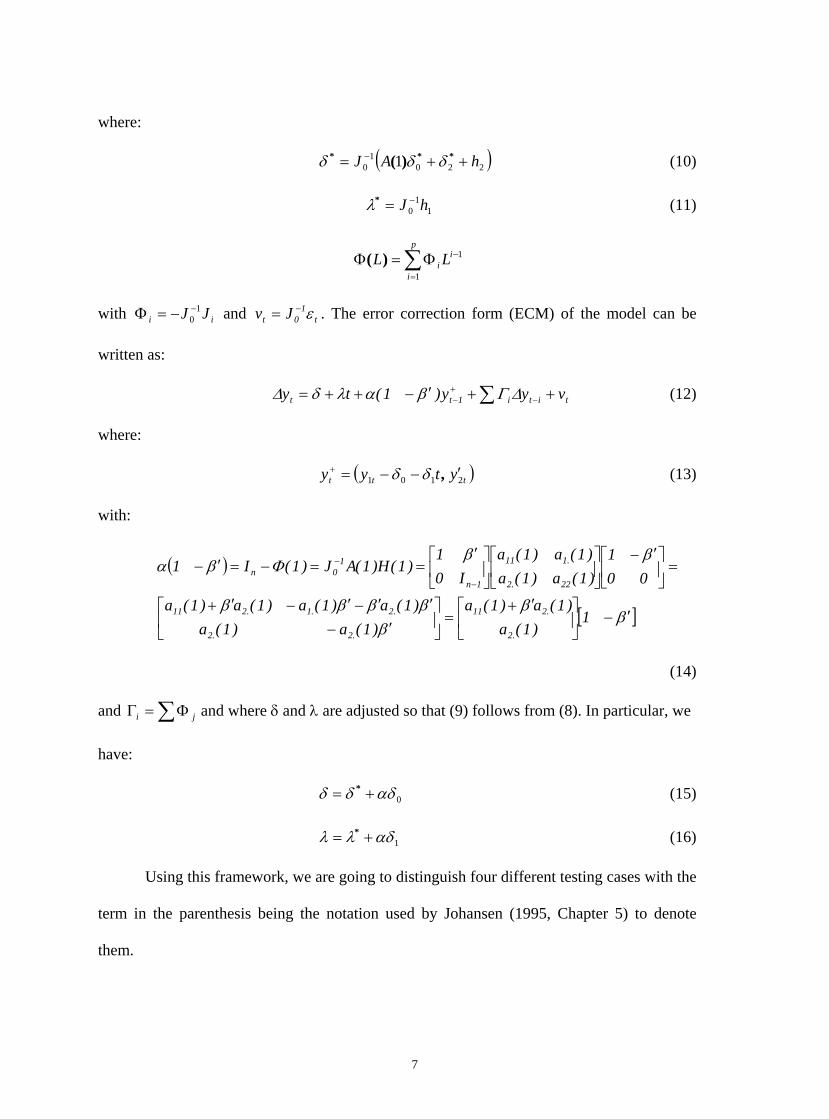
t vy)L(ty +++= −Φλδ (9)

6

where:

( )2201

0 1 hAJ ++= − *** )( δδδ (10)

11

0 hJ −=*λ (11)

∑=

−Φ=Φp

i

ii LL

1

1)(

with and . The error correction form (ECM) of the model can be

written as:

ii JJ 10−−=Φ t

10t Jv ε−=

∑ ++′−++= −+− titi1tt vyy)1(ty ∆Γβαλδ∆ (12)

where:

( )ttt ytyy 2101 ′−−=+ ,δδ (13)

with:

( )

[ ]ββ

βββββ

ββΦβα

′−⎥⎦

⎤⎢⎣

⎡ ′+=⎥

⎦

⎤⎢⎣

⎡′−

′′−′−′+

=⎥⎦

⎤⎢⎣

⎡ ′−⎥⎦

⎤⎢⎣

⎡⎥⎦

⎤⎢⎣

⎡ ′==−=′−

−

−

1)1(a

)1(a)1(a)1(a)1(a

)1(a)1(a)1(a)1(a

001

)1(a)1(a)1(a)1(a

I01

)1(H)1(AJ)1(I1

.2

.211

.2.2

.2.1.211

22.2

.111

1n

10n

(14)

and and where δ and λ are adjusted so that (9) follows from (8). In particular, we

have:

∑Φ=Γ ji

0αδδδ += * (15)

1αδλλ += * (16)

Using this framework, we are going to distinguish four different testing cases with the

term in the parenthesis being the notation used by Johansen (1995, Chapter 5) to denote

them.

7

CASE 1: 0210 === δδδ . Variables around a constant mean; no constant and no linear

trend in the cointegration relation (H2(r)).

In this case, the model is that written in (12), with:

00 == λδ , and tt yy =+

CASE 2: 00 210 ==≠ δδδ ; . Variables around a constant mean; a non-zero constant and

no linear trend in the cointegration relation (H1*(r)).

)y,y(y

)(AJ

ttt

*

201

001

0

01

′−=′=

+=

+

−

δ

λαδδδ

CASE 3: 000 210 ≠=≠ δδδ ,; . Variables around a cointegrated linear trend; a non-zero

constant and no linear trend in the cointegration relation (H1(r)).

In this case,

)y,y(y

))(A(J

ttt

**

201

0201

0

01

′−=′=

++=

+

−

δ

λαδδδδ

CASE 4: 0,0;0 210 ≠≠≠ δδδ . Variables around a non-cointegrated linear trend; a non-

zero constant and a linear trend in the cointegration relation (H*(r)).

In this case, the model is the general model derived previously with as defined in

(12) and δ and λ as defined in (15) and (16), respectively.

+ty

3.- TESTING PROCEDURES

In this section, we propose testing procedures for each of the four cases contemplated

in the previous Section 2. The proof of the asymptotic properties of the proposed tests-

8

statistics will be derived in the first case and then extended, without proof, to the other three

cases.

CASE 1: 0210 === δδδ

Using the restrictions corresponding to this case, we rewrite (1) and the first relation

of (12), respectively, as:

t1t2t1 uyy +′= β (17)

∑∑=

−

=−− ++=

n

1i

1p

1jt1jitij11t1t1 vyuy ∆γα∆ (18)

Let M1 and M2 be two models defined by the following sets of regressors:

{ }{ }jit

jitt

y:M

p,...,,j,n,...,iy,u:M

−

−−

∆

−==∆

2

111 1211

Note that under the null hypothesis, u1t-1 is an I(0) process while, under the alternative,

u1t-1 is an I(1) process. Thus, when we compare M1 and M2 , the first model has an I(0)

variable as the first regressor when the data are generated by the null hypothesis while M1

has an I(1) process as the first regressor when the data are generated by the alternative

hypothesis.

In this paper, we develop a procedure to compare M1 to M2 such that the first regressor of

M1 is always an I(0) process no matter which hypothesis generates the data. To that end, the

first regressor of M1 is defined as a sum of two terms in such a way that when the data are

generated by the null hypothesis the first regressor is dominated by the first term while when

the data are generated by the alternative hypothesis, this first regressor is dominated by the

second term.

9

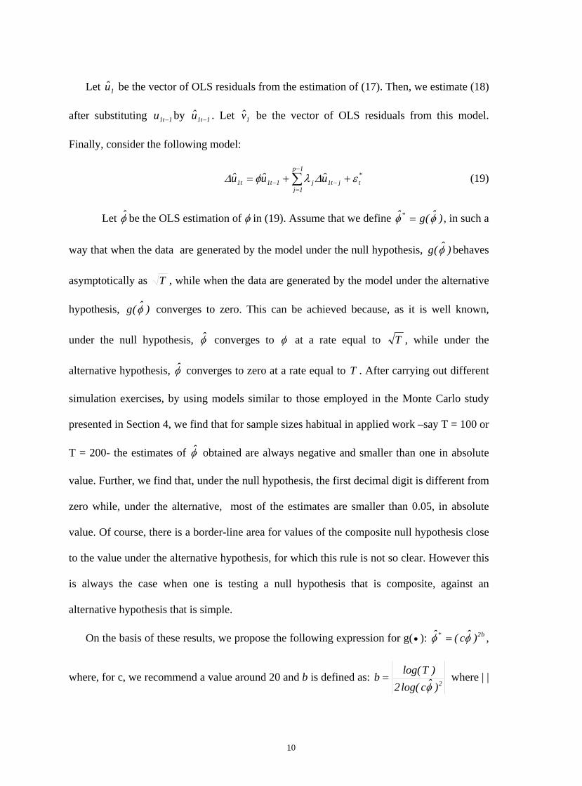
Let be the vector of OLS residuals from the estimation of (17). Then, we estimate (18)

after substituting by . Let be the vector of OLS residuals from this model.

Finally, consider the following model:

1u

1t1u − 1t1u − 1v

∑−

=−− ++=

1p

1j

*tjt1j1t1t1 uuu ε∆λφ∆ (19)

Let φ be the OLS estimation of φ in (19). Assume that we define )ˆ(gˆ * φφ = , in such a

way that when the data are generated by the model under the null hypothesis, )ˆ(g φ behaves

asymptotically as T , while when the data are generated by the model under the alternative

hypothesis, )ˆ(g φ converges to zero. This can be achieved because, as it is well known,

under the null hypothesis, φ converges to φ at a rate equal to T , while under the

alternative hypothesis, φ converges to zero at a rate equal to T . After carrying out different

simulation exercises, by using models similar to those employed in the Monte Carlo study

presented in Section 4, we find that for sample sizes habitual in applied work –say T = 100 or

T = 200- the estimates of φ obtained are always negative and smaller than one in absolute

value. Further, we find that, under the null hypothesis, the first decimal digit is different from

zero while, under the alternative, most of the estimates are smaller than 0.05, in absolute

value. Of course, there is a border-line area for values of the composite null hypothesis close

to the value under the alternative hypothesis, for which this rule is not so clear. However this

is always the case when one is testing a null hypothesis that is composite, against an

alternative hypothesis that is simple.

On the basis of these results, we propose the following expression for g( • ): b2* )ˆc(ˆ φφ = ,

where, for c, we recommend a value around 20 and b is defined as: 2)ˆc

log(log(2

)Tφ

=b where | |

10

denotes absolute value. For these values of b and c, given the values taken by φ it is clear

that, under the null hypothesis, we obtain 1ˆc >φ , while under the alternative hypothesis, we

have that 1ˆc <φ . Hence, defining *φ as b2)ˆc( φ , *φ satisfies the limiting behaviour

assumed for g( ). •

Consider the two following sets of regressors:

)y,...,y,y,...,y,uuˆ(x 1pt21t21pt11t1*t11t1

*t +−−+−−− ′′+=′ ∆∆∆∆φ (20)

)ˆ( **ttt yuz 1∆+= φ (21)

where and are artificial generated variables with mean zero and variance . Note

that x

*tu *

t1u 2*σ

t has n(p-1)+1 elements and that z t has only one. It can be seen that under the null

hypothesis, the first regressor of (20) behaves asymptotically as the first term of the sum,

whilst when the data are generated by the alternative, the first regressor behaves

asymptotically following the pattern of the second term. The same can be said about the

regressor written in (21).

If the null hypothesis holds, then note that when we project t1y∆ on the first set of

regressors written in (20), the projection is on the same space spanned by the regressors

under that hypothesis. On the other hand, when we project this increase on the second set of

regressors in (21), if the data are generated by the null hypothesis, we are projecting this

increase on a process without any structure, whilst if the data are generated by the alternative

hypothesis we are projecting t1y∆ on itself.

Let be the same vector defined in (20) after dividing the first term of it by +1x T .

t1t1tt1 v)1(z)1(xy λλλδ∆ −++−= + (22)

11

where 1δ is the vector of the parameters of the model in (18). Notice that, under the

alternative hypothesis, for λ = 0 , this model asymptotically becomes the model written in

(18). The Ordinary Least Square estimator of λ can be written as:

( ) 11 yMzzMzˆ

XX ∆′′= −λ (23)

where z is the 1×T vector of observations of the variable defined in (21),

with X being the T X)XX(XIM X ′′−= −1 × [n(p-1)+1] matrix of observations of the n(p-

1)+1 elements of the vector defined in (20) and 1y∆ is the 1×T vector of observations of

t1y∆ . In the following theorem we derive the asymptotic properties of this estimator.

THEOREM 1: Assume that the DGP is given by (1) and (2) with

0210 === δδδ and that the disturbances follow the same stochastic properties commented

on in the previous section. Then:

⎟⎟⎟⎟

⎠

⎞

⎜⎜⎜⎜

⎝

⎛

⎯→⎯ 2*

2

2*

11

d ,Tv'vlimp

NˆTσσ

σλ (24)

PROOF: See the Appendix.

Thus, we propose the following statistic to test for cointegration:

21111

/X

X*

)zMz(svvyMzJ

′′−∆′

= (25)

where s2 is the OLS estimated residual variance of the regression of t1y∆ on and in

(22).

+tx tz

The asymptotic properties of this statistic under both hypotheses are as follows:

THEOREM 2: under the null hypothesis that there is one cointegration relation, we

have:

12

)1,0(NJ d* ⎯→⎯

Proof: See the Appendix

THEOREM 3: Under he alternative hypothesis that there is no cointegration relation, it

holds that:

∞⎯→⎯*J

Proof: See the Appendix

CASE 2: 00 210 ==≠ δδδ ; .

Here, we follow using the same testing procedure, but adopting it to the new

restrictions. In particular, a constant is included in (17) and (18), while in (18) and (19) we

use ( ) +−′− 11 tyβ instead of . This same change is introduced in (20), where we define x11 −tu t.

Taking into account these modifications, we redefine the J-test written in (25) and the null

hypothesis is rejected when the value of this statistic is over the critical point corresponding

to a Standard Normal distribution once the nominal size is chosen.

CASE 3: 000 210 ≠=≠ δδδ ,; .

Since, in this case, the linear trends of the two variables are cointegrated, the testing

procedure is the same as that commented on for Case 2.

CASE 4: 0,0;0 210 ≠≠≠ δδδ .

The modifications to be introduced in this case are as follows: a constant and a linear

trend should be included in (17) and (18), while in (18) and (19) we use (13) to define u1t-1.

Introducing these changes in (25), the new J-test is obtained and the corresponding critical

region is derived from the Standard Normal distribution.

13

By using the triangular form of the system of Phillips (1991) and Phillips and

Loretan (1991), the extension of the testing procedure just commented to situations whith

more than one cointegration relation is straightforward.

4. MONTE CARLO STUDY

This section is dedicated to presenting the results from a Monte Carlo simulation study.

Considering a model with two variables, we analyze the behaviour of the test proposed in this

paper for the four cases introduced in the previous sections.

Two broad approaches have been followed in the literature in order to evaluate the

performance of different cointegration testing procedures using Monte Carlo analysis. The

first, based on a transformation of the model into a “canonical form”, can be seen, for

example, in Toda (1994,1995) and in Hubrich et al. (2001); the second, with a DGP close to

what can be regarded as a “structural form”, has been used in Haug (1996), who follows the

same framework used in Gonzalo (1994), among others. In this section, we assume a model

close to this second approach.

In the study, we test for the null hypothesis that the rank of the cointegration space is one,

as against the alternative hypothesis that the rank is zero, i. e., H0: r = 1 against H1: r = 0.

We assume that the data are generated by the following model:

t1t210t1 uyty +++= βδδ (26)

t2t2 uy =∆ (27)

with

t12t1121t111t1 uuu ερρ ++= −− (28)

t21t222t2 uu ερδ ++= − (29)

14

and ~N(0, iidt2

t1t ⎟⎟

⎠

⎞⎜⎜⎝

⎛=

εε

ε )Σ , with ⎟⎟⎠

⎞⎜⎜⎝

⎛= 2

2

21021

σσσρσ

Σ

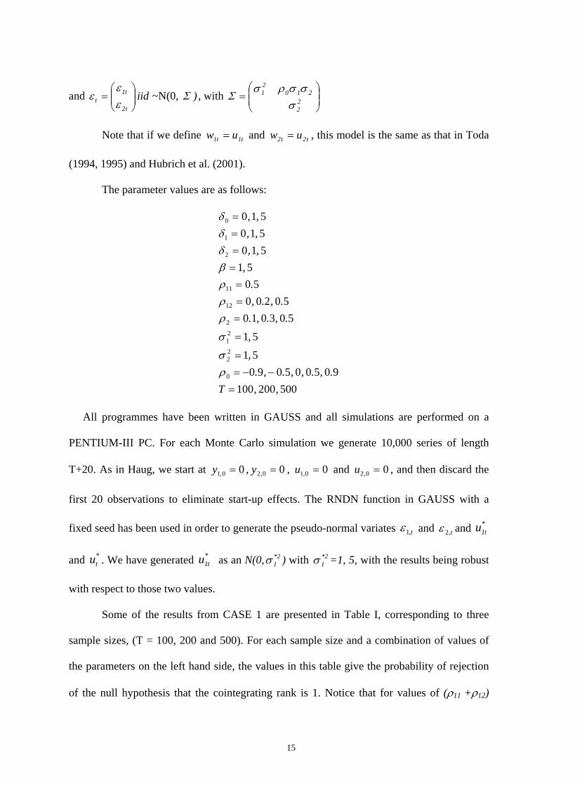
Note that if we define and t1t1 uw = t2t2 uw = , this model is the same as that in Toda

(1994, 1995) and Hubrich et al. (2001).

The parameter values are as follows:

500200100905005090

5151

50301050200

5051

510510510

0

22

21

2

12

11

2

1

0

,,T.,.,,.,.

,,

.,.,..,.,

.,

,,,,,,

=−−=

=

=

===

====

ρσ

σ

ρρρβδδδ

All programmes have been written in GAUSS and all simulations are performed on a

PENTIUM-III PC. For each Monte Carlo simulation we generate 10,000 series of length

T+20. As in Haug, we start at 00,1 =y , 00,2 =y , u1 0 0, = and u2 0 0, = , and then discard the

first 20 observations to eliminate start-up effects. The RNDN function in GAUSS with a

fixed seed has been used in order to generate the pseudo-normal variates ε1,t and ε 2,t and

and . We have generated as an N(0, ) with =1, 5, with the results being robust

with respect to those two values.

*t1u

*tu *

t1u 2*1σ 2*

1σ

Some of the results from CASE 1 are presented in Table I, corresponding to three

sample sizes, (T = 100, 200 and 500). For each sample size and a combination of values of

the parameters on the left hand side, the values in this table give the probability of rejection

of the null hypothesis that the cointegrating rank is 1. Notice that for values of (ρ11 +ρ12)

15

smaller than one, the values in the table give the empirical size, while for (ρ11 +ρ12) = 1, these

values give account of the power. A 5% nominal size has been used in all cases.

TABLE I

From an examination of the values, we can appreciate that the empirical size is close

to the nominal size, even for small sample sizes. The power, although not very high in small

samples, increases as expected, as the sample size increases. Moreover, the results are robust

with respect to changes of ρ0 , ρ2 and , i = 1, 2. 2iσ

The results for CASE 2 are presented in Table II. As in the previous case, they make

clear that the empirical size is close to the nominal 5% size in almost every case. Further,

they appear to cofirm that when (ρ11 +ρ12) = 1, the power is rather low for small sample sizes.

However, the power increases as the sample size grows and approach unity when T = 500.

TABLE II

The same conclusions are derived from Table III, CASE 3, and Table IV, CASE 4:

empirical size close to the 5% nominal size and low power for samples around T = 100;

however, this power increases as the sample size grows, although at a slower rate than in the

two previous cases:

TABLE III

TABLE IV

16

5.- CONCLUSIONS

This paper has been dedicated to deriving a test procedure for testing cointegration that,

under the null hypothesis, follows a Standard Normal distribution. To that end, we have considered

four alternative specifications, depending on the form adopted by the deterministic terms.

The test procedure has been based on the comparison of the form adopted by a relation of

the Error Correction Form, under the null hypothesis that there is one coitegration relation, with

respect to the form adopted by that relation when it is assumed that there is no cointegraion. Since

the form corresponding to the case with cointegration has one regressor that behaves as an I(0)

process under the null hypothesis, and as an I(1) process under the alternative hypothesis, we have

defined a new set of regressors in which one of them is defined in terms of the sum of the two

elements in such a way that the I(0) character of the regressor is maintained no matter which

hypothesis generates the data.

By using these new set of regressors, we have derived the cointegration testing procedure

in Section 3 and it has been shown that the procedure, under the null hypothesis, follows a

standard Normal distribution.

In the closing section of the paper, we have considered the results from some Monte-Carlo

simulations. For a wide range of values of the parameters of the model, it has been shown that the

proposed test has a good performance, both in terms of how close the empirical size is to the

nominal size, and in terms of the high power values.

REFERENCES

Davidson, J. E. H., D. F.Hendry, F. Srba & S.Yeo (1978) Econometric modelling of the

aggregate time-series relationship between consumers expenditure and income in the united

kingdom. Economic Journal 88, 661-692.

17

Davidson, R. & J. G. MacKinnon (1981) Several tests for model specification in the presence

of alternative hypotheses. Econometrica 46,781-793.

Engle, R. F. & C. W. J. Granger (1987) Cointegration and error-correction: representation,

estimation and testing. Econometrica 55, 251-276.

Ericson, N. R. & J. G. MacKinnon (2002) Distribution of error correction tests for

cointegration. Econometrics Journal 5, 285-318.

Gonzalo, J. (1994) Five alternative methods of estimating long-run equilibrium relationships.

Journal of Econometrics 60, 203-233.

Hamilton, J. D. (1994) Time Series analysis. Princenton University Press. New Jersey.

Harbo, I., S. Johansen, B. Nielsen & A. Rahbek (1998) Asymptotic inference on cointegrating

rank in partial systems. Journal of Business and Economic Statistics 16, 4, 388-399.

Haug, A. A. (1996) Tests for cointegration: a Monte Carlo comparison. Journal of

Econometrics 71, 89-115.

Hubrich, K., H. Lütkepohl & P. Saikkonen (2001) A review of systems cointegration tests.

Econometrics Review 20 (3), 247-318.

Johansen, S. (1988) Statistical analysis of cointegrating vectors. Journal of Economic

Dynamics and Control 12, 231-254.

Johansen, S. (1995) Likelihood-based inference in cointegrated vector autoregressive models.

Oxford University Press.

Phillips, P. (1991) Optimal inference in cointegrated ssystems. Econometrica, 59, 283-306.

Phillips, P. and Loretan, M. (1991) Estimating long-run economic equilibria. Review of

Economic Studies, 58,99-125.

18

Sargan, J. D. (1964) Wages and prices in the United Kingdom: a study. In P. E. Hart, G. Mills

& J. K. Whitaker (eds.), Econometric Methodology, Econometric Analysis for National Economic

Planning, vol.16 of Colston Papers, 25-54. London: Butterworths.

Toda, H. Y. (1994) Finite sample properties of likelihood ratio tests for cointegration ranks

when linear trends are present. Review of Economics and Statistics 76, 66-79.

Toda, H. Y. (1995) Finite sample performance of likelihood ratio tests for cointegration ranks

in vector autoregressions. Econometric Theory 11, 1015-1032.

APPENDIX

First, some preliminary results, useful when proving the three theorems, are collected

in the following lemma.

LEMMA1: Let the DGP be (1)-(2) with 0,0,0 210 === δδδ . Then:

(i) t1p

t1 uu ⎯→⎯

(ii) ⎟⎟⎠

⎞⎜⎜⎝

⎛=⎯→⎯′ −−

1110

0100p12

11 Qq

qqQXHXH

(iii) QXXH p*1

12 ⎯→⎯′−

(iv) is OzXH 12 ′−

p(1)

(v) )1(OzzM pp

x +⎯→⎯

(vi) 2*pX2 zMz

T1 σ⎯→⎯′

where H1 and H2 are, respectively:

⎟⎟⎠

⎞⎜⎜⎝

⎛=

− )1p(n

2/1

1 I00T

H and ⎟⎟⎠

⎞⎜⎜⎝

⎛=

− )1p(n

2/3

2 TI00T

H

19

and where Q is a square matrix of constants of order n(p-1)+1, is the matrix of

observations of the regressors in (18) and δ

*1X

1 is the vector of n(p-1)+1 parameters of these

regressors.

PROOF:

(i) Write as: tu1

t2t1t2t1t1 y)ˆ(uyˆyu βββ −−=−=

where β is the Ordinary Least Square estimator of β: ∑

∑=t2

t2t1

yyy

β . Since, when the

variables are cointegrated, ( β -β) is Op(T-1), then the result follows.

(ii) Let X be partitioned as )Xx(X 10= , where x0 is the 1T × vector of

observations of the first element of xt and X1 is the )1p(nT −× matrix of observations of

the rest of elements of xt. The term on the left hand side of (ii) can be written as:

⎟⎟⎟⎟

⎠

⎞

⎜⎜⎜⎜

⎝

⎛

′

′′

=′ −−

TXX

TXx

Txx

XHXH11

2/310

200

12

11 (A.1)

The convergence of the (1,1) element of this matrix is:

∑ ∑ ∑ −− ++=′ *

t11t1*

22*t12

21t1

2*22

00 uuˆ2T1u

T1uˆ

T1

Txx

φφ

and, since, as we have already stated, Tˆ 2* ≈φ and T≈*φ (asymptotically), by using (i) we

have that:

00p

200 q)0(

Txx

1=⎯→⎯

′γ (A.2)

which is the variance of u1t.

20

The asymptotic convergence of the i-th generic element of 2/310

TXx′

is, for i = 1, 2, ...,n

and j = 1,...,p-1:

)1j(T

yu

yuT

1yuˆT

1yxT

1

i,1 yupjit1t1

pjit

*t2/3jit1t1

*2/3jitt02/3

−⎯→⎯

⎯→⎯+=

∑

∑∑∑

−−

−−−−

∆γ∆

∆∆φ∆ (A.3)

With respect to the convergence of the ij-th element of T

XX 11′ , we have that:

)jk(T

yyli y,y

pkltjit −⎯→⎯∑ −−∆∆γ

∆∆ (A.4)

(iii) The left hand side term of this expression can be written as:

⎥⎥⎥⎥

⎦

⎤

⎢⎢⎢⎢

⎣

⎡

∆′

∆′′

=′

−

−

TYX....

TYx

Tux

XXH//

,

*

1

230

23110

11

2 (A.5)

The convergence of 2/31,10

Tux −′

is as follows:

00p

1t1*t12/31t11t1

*2/3 quu

T1uuˆ

T1

⎯→⎯⎟⎠⎞

⎜⎝⎛ + ∑∑ −−−φ (A.6)

using (i) and the fact that Tˆ* ≈φ .

The convergence of 2/30

TYx ∆′

and T

YX ∆′1 is straightforward, because YX 1 ∆=′ .

(iv) We have that:

11

2**1

21

2 yXHuXˆHzXH ∆φ ′+′=′ −−− (A.7)

Note that

11

21*1

1211

*1

121

12 vXHXXH)vX(XHyXH ′+′=+′=′ −−−− δδ∆ (A.8)

21

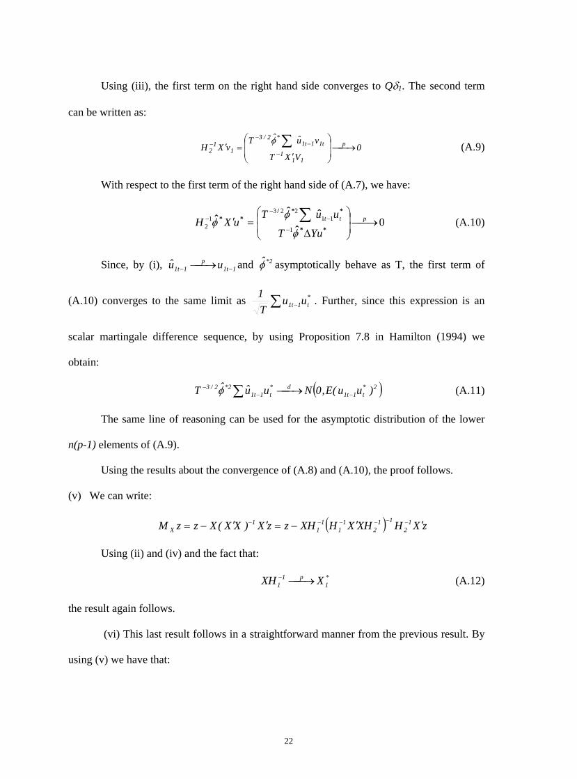
Using (iii), the first term on the right hand side converges to Qδ1. The second term

can be written as:

0VXT

vuˆTvXH p

111

t11t1*2/3

11

2 ⎯→⎯⎟⎟

⎠

⎞

⎜⎜

⎝

⎛

′=′

−

−−

− ∑φ (A.9)

With respect to the first term of the right hand side of (A.7), we have:

01

11223

12 ⎯→⎯⎟

⎟⎠

⎞⎜⎜⎝

⎛

∆=′

−

−−

− ∑ ptt

YuT

uuTuXH

**

**/**

ˆˆˆ

ˆφ

φφ (A.10)

Since, by (i), and 1t1p

1t1 uu −− ⎯→⎯ 2*φ asymptotically behave as T, the first term of

(A.10) converges to the same limit as ∑ −*t1t1 uu

T1 . Further, since this expression is an

scalar martingale difference sequence, by using Proposition 7.8 in Hamilton (1994) we

obtain:

( )2*t1t1

d*t1t1

2*2/3 )uu(E,0NuuˆT −−− ⎯→⎯∑φ (A.11)

The same line of reasoning can be used for the asymptotic distribution of the lower

n(p-1) elements of (A.9).

Using the results about the convergence of (A.8) and (A.10), the proof follows.

(v) We can write:

( ) zXHXHXHXHzzX)XX(XzzM 12

112

11

11

1X ′′−=′′−= −−−−−−

Using (ii) and (iv) and the fact that:

*1

p11 XXH ⎯→⎯− (A.12)

the result again follows.

(vi) This last result follows in a straightforward manner from the previous result. By

using (v) we have that:

22

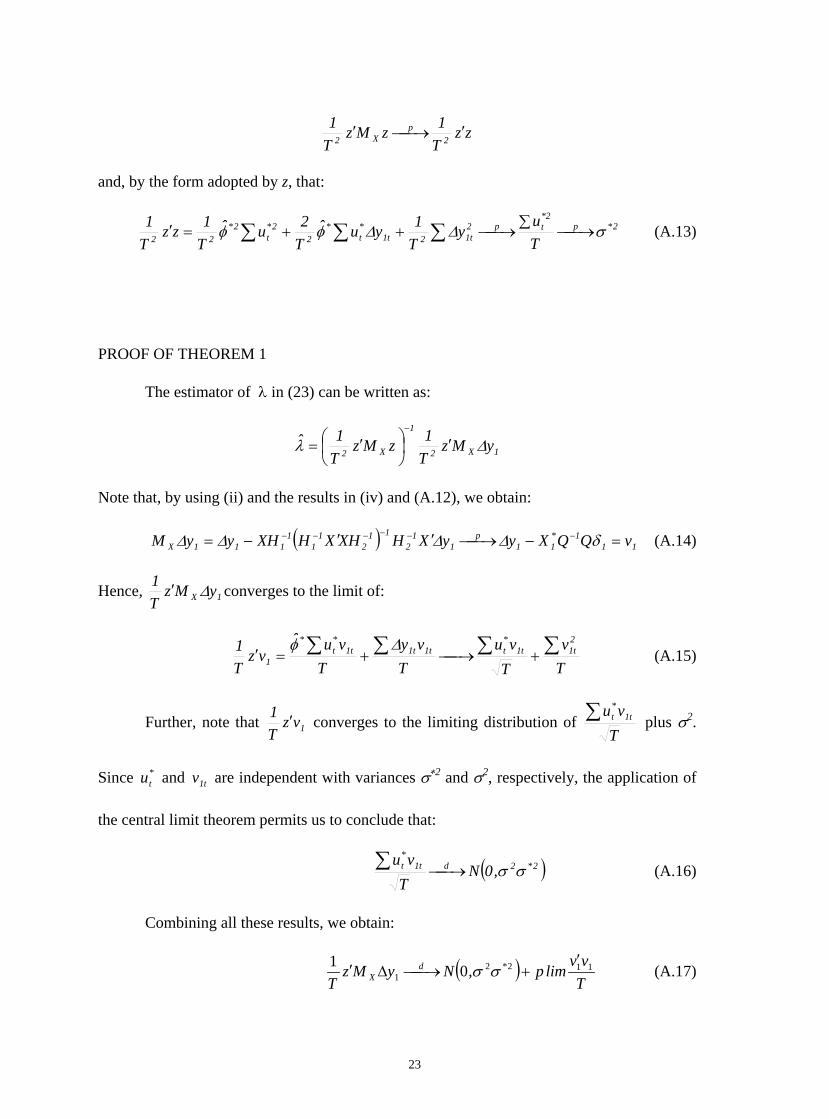
zzT1zMz

T1

2p

X2′⎯→⎯′

and, by the form adopted by z, that:

2*p2*

tp2t12t1

*t

*2

2*t

2*22 T

uy

T1yuˆ

T2uˆ

T1zz

T1 σ∆∆φφ ⎯→⎯∑⎯→⎯++=′ ∑∑∑ (A.13)

PROOF OF THEOREM 1

The estimator of λ in (23) can be written as:

1X2

1

X2 yMzT1zMz

T1ˆ ∆λ ′⎟

⎠⎞

⎜⎝⎛ ′=

−

Note that, by using (ii) and the results in (iv) and (A.12), we obtain:

( ) 111*

11p

11

211

21

11

111X vQQXyyXHXHXHXHyyM =−⎯→⎯′′−= −−−−−− δ∆∆∆∆ (A.14)

Hence, 1X yMzT1 ∆′ converges to the limit of:

Tv

Tvu

Tvy

Tvuˆ

vzT1 2

t1t1*tt1t1t1

*t

*

1∑∑∑∑ +⎯→⎯+=′

∆φ (A.15)

Further, note that 1vzT1 ′ converges to the limiting distribution of

Tvu t1

*t∑ plus σ2.

Since and are independent with variances σ*tu t1v ∗2 and σ2, respectively, the application of

the central limit theorem permits us to conclude that:

( 2*2dt1*t ,0NT

vuσσ⎯→⎯ )∑ (A.16)

Combining all these results, we obtain:

( )Tvvlimp,NyMz

T*d

X1122

1 01 ′+⎯→⎯∆′ σσ (A.17)

23

By using (vi), the result is:

⎟⎟⎟⎟

⎠

⎞

⎜⎜⎜⎜

⎝

⎛ ′

⎯→⎯′⎟⎠⎞

⎜⎝⎛ ′=

−

2*

2

2*

11

d1X

1

X2 ,Tvvlimp

NyMzT1zMz

T1ˆT

σσ

σ∆λ (A.18)

PROOF OF THEOREM 2:

We have:

( )

)1,0(N

TzMz

sTvv

TzMzˆT

TzMzs

TzMz

Tvv

TzMz

yMzT1

TzMz

zMzsvvyMzJ

d

2/1

2X

111

2X

2/1

2X

1

2X

111

2X

1x

1

2X

2/1X

111X

⎯→⎯

⎟⎠⎞

⎜⎝⎛ ′

′⎟⎠⎞

⎜⎝⎛ ′

−=

=

⎟⎠⎞

⎜⎝⎛ ′

⎟⎠⎞

⎜⎝⎛ ′

′⎟⎠⎞

⎜⎝⎛ ′

−′⎟⎠⎞

⎜⎝⎛ ′

=′

′−′=

−

−

−−

λ

∆∆

By using (vi) and the fact that, under the null hypothesis, 21111 σ⎯→⎯′

⎯→⎯′ pp

Tvv

Tvv and

, the proof follows. 2p2s σ⎯→⎯

PROOF OF THEOREM 3

Here, the proof follows because, under the alternative hypothesis, 1X yMzT1 ∆′ and

Tvv 11′ converge to different limits, and furthermore, because 0s p2 ⎯→⎯ t1y∆ is projected on

itself.

24

TABLE I: CASE 1: 0210 === δδδ

SIZE AND POWER OF THE TEST WHEN THE COINTEGRATION RANK IS r = 1 (ρ12 =0,

0.2) OR r =0 (ρ12 = 0.5); ( AND 5,1,5.0 2111 === σβρ )12

2 =σ

ρ12 ρ2 ρ0 T = 100 T = 200 T = 500

0 0.1 -0.9 0.117 0.052 0.052 0 0.080 0.053 0.054 0.9 0.065 0.049 0.053 0.3 -0.9 0.112 0.053 0.053 0 0.080 0.053 0.054 0.9 0.064 0.049 0.053 0.2 0.1 -0.9 0.056 0.051 0.052 0 0.055 0.050 0.055 0.9 0.057 0.048 0.053 0.3 -0.9 0.056 0.051 0.053 0 0.055 0.050 0.054 0.9 0.056 0.049 0.053 0.5 0.1 -0.9 0.289 0.489 0.804 0 0.438 0.693 0.886 0.9 0.282 0.494 0.806 0.3 -0.9 0.245 0.420 0.738 0 0.455 0.708 0.881 0.9 0.245 0.426 0.734

25

TABLE II: CASE 2: 00 210 ==≠ δδδ ; .

SIZE AND POWER OF THE TEST WHEN THE COINTEGRATION RANK IS r = 1 (ρ12 =0.

0.2) OR r =0 (ρ12 = 0.5); ( AND 5,1,5.0 2111 === σβρ )12

2 =σ )1( 0 =δ

ρ12 ρ2 ρ0 T = 100 T = 200 T = 500

0 0.1 -0.9 0.081 0.052 0.052 0 0.075 0.050 0.048 0.9 0.058 0.050 0.049 0.3 -0.9 0.061 0.052 0.052 0 0.061 0.050 0.047 0.9 0.058 0.050 0.048 0.2 0.1 -0.9 0.054 0.050 0.052 0 0.058 0.050 0.048 0.9 0.056 0.049 0.048 0.3 -0.9 0.054 0.051 0.052 0 0.056 0.050 0.048 0.9 0.055 0.048 0.049 0.5 0.1 -0.9 0.205 0.469 0.897 0 0.195 0.465 0.901 0.9 0.198 0.459 0.899 0.3 -0.9 0.193 0.468 0.895 0 0.197 0.466 0.900 0.9 0.195 0.457 0.902

26

TABLE III: CASE 3: 0,0;0 210 ≠≠= δδδ

SIZE AND POWER OF THE TEST WHEN THE COINTEGRATION RANK IS

r = 1 (ρ12 =0. 0.2) OR r =0 (ρ12 = 0.5); ( AND5,1,5.0 2111 === σβρ )12

2 =σ )1,1( 21 == δδ

ρ12 ρ2 ρ0 T = 100 T = 200 T = 500

0 0.1 -0.9 0.085 0.054 0.054 0 0.080 0.053 0.048 0.9 0.062 0.050 0.048 0.3 -0.9 0.061 0.053 0.053 0 0.063 0.052 0.048 0.9 0.061 0.049 0.049 0.2 0.1 -0.9 0.055 0.054 0.054 0 0.059 0.052 0.048 0.9 0.059 0.049 0.049 0.3 -0.9 0.055 0.051 0.052 0 0.057 0.051 0.048 0.9 0.058 0.050 0.049 0.5 0.1 -0.9 0.219 0.472 0.883 0 0.194 0.453 0.886 0.9 0.208 0.462 0.882 0.3 -0.9 0.198 0.466 0.884 0 0.202 0.458 0.887 0.9 0.198 0.448 0.881

27

TABLE IV: CASE 4: 0,0;0 210 ≠≠≠ δδδ

SIZE AND POWER OF THE TEST WHEN THE COINTEGRATION RANK IS

r = 1 (ρ12 =0. 0.2) OR r =0 (ρ12 = 0.5); ( AND 5,1,5.0 2111 === σβρ )12

2 =σ

)1,1,1( 210 === δδδ

ρ12 ρ2 ρ0 T = 100 T = 200 T = 500

0 0.1 -0.9 0.069 0.056 0.054 0 0.082 0.053 0.048 0.9 0.059 0.049 0.048 0.3 -0.9 0.060 0.053 0.053 0 0.066 0.052 0.048 0.9 0.060 0.049 0.048 0.2 0.1 -0.9 0.056 0.056 0.054 0 0.060 0.053 0.048 0.9 0.057 0.049 0.048 0.3 -0.9 0.055 0.052 0.053 0 0.057 0.052 0.048 0.9 0.057 0.049 0.049 0.5 0.1 -0.9 0.123 0.270 0.788 0 0.089 0.242 0.793 0.9 0.091 0.247 0.790 0.3 -0.9 0.095 0.254 0.787 0 0.090 0.242 0.793 0.9 0.090 0.241 0.786

28