Energy consumption and GDP in Italy: cointegration and causality analysis

Energy consumption and GDP in Italy: cointegrationand causality analysis

Cosimo Magazzino

Received: 4 January 2014 / Accepted: 16 April 2014 / Published online: 30 April 2014� Springer Science+Business Media Dordrecht 2014

Abstract The aim of this article was to assess the empirical evidence of the nexus

between GDP and energy consumption for Italy during the period 1970–2009, using a time

series approach. After a brief introduction, a survey of the economic literature on this issue

is shown, before discussing the data and introducing some econometric techniques. Sta-

tionarity tests reveal that both series are nonstationary, or I(1). Moreover, a cointegration

relationship is found between the two variables. The short-run dynamics of the variables

show that the flow of causality runs from energy use to GDP, and there is a long-run

bidirectional causal relationship (or feedback effect) between the two series. Consequently,

we conclude that energy is a limiting factor to GDP growth in Italy and that energy

conservation policy should be formulated and implemented wisely.

Keywords Energy policies � Energy consumption � GDP � Stationarity �Cointegration � Causality � Italy

JEL Classification B22 � C22 � N54 � Q43

1 Introduction

The causal relation between energy consumption and economic growth has been a well-

studied topic. Energy is one of the essential factors for any country’s economic

C. Magazzino (&)Department of Political Sciences, Roma Tre University, Via G. Chiabrera 199, 00145 Rome, Italye-mail: [email protected]

C. MagazzinoItalian Economic Association (SIE), Ancona, Italy

C. MagazzinoRoyal Economic Society (RES), London, UK

123

Environ Dev Sustain (2015) 17:137–153DOI 10.1007/s10668-014-9543-8

development and therefore plays an important role in economic activities: energy demand

and supply and pricing impact on the socioeconomic development, the living standards,

and the overall quality of life of the people (Iwayemi 1998). On the other hand, higher

level of economic development could induce more energy consumption.

Over the past three decades, many studies—using the concepts of cointegration and

Granger causality—focused on several countries and time period. Since the pioneering

study by Kraft and Kraft (1978), empirical findings are mixed and, for some countries,

controversial (Ozturk 2010). The results differ even on the direction of causality and the

short-term versus long-term effects on energy policies. Depending upon what kind of

causal relationship exists, its policy implications may be significant (Dakhlaoui et al.

2012).

GDP and energy consumption of developing countries are increasing exponentially,

whereas GDP and energy consumption of developed countries are increasing linearly.

Because of the international goal of curbing the increase in global temperature to a

maximum of 2 �C in the context of global warming, governments are interested in studying

the relationship between energy consumption and GDP. To achieve this goal, it has

become necessary to assess the impacts of policies that promote energy conservation and

efficiency on national GDP and economic growth. According to the International Energy

Agency (IEA), ‘‘80 % of emissions from the energy sector that were planned for 2020 have

already been reached and 40 % of CO2 emissions from OECD countries.’’ This accelerated

trend in global emissions represents a step backward in the battle against global warming

(Campo and Sarmiento 2013).

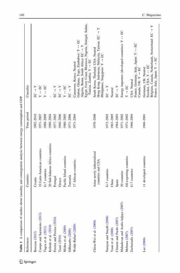
Moreover, multiple causality studies have been done for many countries in the world;

however, few studies have been devoted to the analysis of this nexus for the Italian case:

Erol and Yu (1987), Soytas and Sari (2003, 2006), Lee (2006), Zachariadis (2007), Lee and

Chang (2007), Chontanawat et al. (2008), Narayan and Smyth (2008), Tugcu et al. (2012),

and Magazzino (2014a, b).

In Italy, gas and oil are by far the largest sources of primary energy (around 77 % of the

total). Thus, qualitatively, we would expect that a decline in energy production would be

accompanied by a decline in GDP.

Therefore, this paper examines the nexus between real per capita GDP and per capita

energy consumption in Italy for the period 1970–2009, using time series methodologies on

stationarity, cointegration, and causality. The results might help to define and implement

the appropriate energy development policies in Italy. The data used in our empirical

analyses are obtained by Total Economy Database (TED) and International Energy Agency

(IEA).

Besides the Introduction, the outline of this paper is as follows. Section 2 provides a

survey of the economic literature on the nexus between energy consumption and GDP.

Section 3 contains an overview of the applied empirical methodology and a brief dis-

cussion of the data used. Section 4 discusses our empirical results. Section 5 presents some

concluding remarks, and finally, Sect. 6 gives suggestions for future researches.

2 The nexus between energy consumption and GDP

The directions of the causality relationship between energy consumption and domestic

product may be categorized into four types, each of which has important implications for

energy policy (Apergis and Payne 2009; Cheng et al. 2007; Payne 2009).

138 C. Magazzino

123

As explained in Ozturk (2010), which contains a detailed literature review, we can have

the following:

• Neutrality hypothesis: If no causality exists between GDP and energy consumption, it

implies that energy consumption is not correlated with GDP. The absence of Granger

causality supports the neutrality hypothesis as documented by Akarca and Long (1980),

Yu and Hwang (1984), Yu and Choi (1985), Erol and Yu (1987), Yu and Jin (1992),

Cheng (1995), Masih and Masih (1996), Glasure and Lee (1997), Fatai et al. (2002),

Soytas and Sari (2003), Altinay and Karagol (2004), Chontanawat et al. (2006), Jobert

and Karanfil (2007), Lee (2006), Soytas et al. (2007), Zachariadis (2007), Chiou-Wei

et al. (2008), Karanfil (2008), Yuan et al. (2008), Halicioglu (2009), Payne (2009),

Soytas and Sari (2009), and Wolde-Rufael (2009).

• Conservation hypothesis: the unidirectional causality running from GDP to energy

consumption. This hypothesis has found empirical supports in Kraft and Kraft (1978),

Abosedra and Baghestani (1989), Masih and Masih (1996), Cheng and Lai (1997),

Cheng (1997, 1999), Soytas et al. (2001), Aqeel and Butt (2001), Soytas and Sari

(2003, 2006), Lee (2006), Zachariadis (2007), Zamani (2007), Mehrara (2007), Lise

and Van Montfort (2007), Lee and Chang (2007), Chiou-Wei et al. (2008), Ang (2008),

Zhang and Cheng (2009), and Wolde-Rufael (2009).

• Growth hypothesis: the unidirectional causality running from energy consumption to

GDP. This hypothesis is in line with the empirical findings in Stern (1993), Masih and

Masih (1996), Glasure and Lee (1997), Stern (2000), Asafu-Adjaye (2000), Soytas and

Sari (2003), Wolde-Rufael (2004), Thoma (2004), Lee (2005), Lee and Chang (2005),

Soytas and Sari (2006), Lee (2006), Lee and Chang (2007), Ho and Siu (2007), Climent

and Pardo (2007), Ang (2007), Narayan and Smyth (2008), Chiou-Wei et al. (2008),

Wolde-Rufael (2009), Odhiambo (2009), Tsani (2010), Pereira and Pereira (2010), and

Borozan (2013).

• Feedback hypothesis: If there exists a bidirectional causality flow between GDP and

energy consumption, the feedback hypothesis is shown by Hwang and Gum (1991),

Masih and Masih (1996, 1997), Asafu-Adjaye (2000), Yang (2000), Hondroyiannis

et al. (2002), Glasure (2002), Soytas and Sari (2003), Paul and Bhattacharya (2004), Oh

and Lee (2004a, 2004b), Ghali and El-Sakka (2004), Soytas and Sari (2006), Lee

(2006), Zachariadis (2007), Mahadevan and Asafu-Adjaye (2007), Erdal et al. (2008),

Belloumi (2009), Mishra et al. (2009), Wolde-Rufael (2009), Tugcu et al. (2012), and

Campo and Sarmiento (2013).

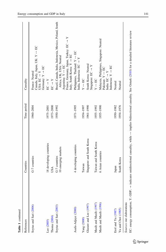
Table 1 above presents a concise overview on causality between GDP and energy

consumption discussed in several studies on this topic.

3 Econometric methodology and data

In this research, we use time series econometric analysis. In particular, the VAR (Vector

AutoRegressive) and VEC (Vector Error Correction) models were used.1

Most of time series have unit root as many studies indicated, including Nelson and

Plosser (1982), and as proved by Stock and Watson (1988) and Campbell and Perron

(1991) among others that most of the time series are nonstationary. The presence of a unit

1 For detailed analyses of the time series modelling used see, among others: Lutkepohl (2005), Enders(2003), Dagum (2002), Franses (2002), Hamilton (1994).

Energy consumption and GDP in Italy 139

123

Ta

ble

1A

com

par

ison

of

studie

sab

out

causa

lity

and

coin

tegra

tion

anal

ysi

sbet

wee

nen

ergy

consu

mpti

on

and

GD

P

Ref

eren

ces

Co

un

trie

sT

ime

per

iod

Cau

sali

ty

Bo

roza

n(2

01

3)

Cro

atia

19

92–

20

10

EC?

Y

Cam

po

and

Sar

mie

nto

(20

13)

10

Lat

in-A

mer

ican

countr

ies

1971–2007

Y$

EC

Tu

gcu

etal

.(2

01

2)

G-7

cou

ntr

ies

19

80–

20

09

Y$

EC

Keb

ede

etal

.(2

01

0)

20

Su

b-S

ahar

anA

fric

aco

un

trie

s1

98

0–

20

04

–

Per

eira

and

Per

eira

(20

10)

Po

rtu

gal

19

77–

20

03

EC?

Y

Tsa

ni

(20

10)

Gre

ece

19

60–

20

06

EC?

Y

Mis

hra

etal

.(2

00

9)

Pac

ific

Isla

nd

cou

ntr

ies

19

80–

20

05

Y$

EC

Od

hia

mb

o(2

00

9)

Tan

zan

ia1

97

1–

20

06

EC?

Y

Wold

e-R

ufa

el(2

00

9)

17

Afr

ican

cou

ntr

ies

19

71–

20

04

Cam

ero

on,

Ken

ya:

Neu

tral

Gab

on

,G

han

a,T

og

o,

Zim

bab

we:

Y$

EC

Alg

eria

,B

enin

,S

ou

thA

fric

a:E

C?

YE

gy

pt,

Ivo

ryC

oas

t,M

oro

cco,

Nig

eria

,S

eneg

al,

Su

dan

,T

un

isia

,Z

amb

ia:

Y?

EC

Ch

iou-W

eiet

al.

(20

08)

Asi

ann

ewly

indu

stri

aliz

edco

un

trie

san

dU

SA

1970–2000

South

Kore

a,T

hai

land,

US

A:

Neu

tral

Ho

ng

Ko

ng

,In

do

nes

ia,

Mal

aysi

a,T

aiw

an:

EC?

YP

hil

ippin

es,

Sin

gap

ore

:Y

?E

C

Nar

ayan

and

Sm

yth

(20

08)

G-7

cou

ntr

ies

19

72–

20

02

EC?

Y

Yu

anet

al.

(20

08)

Chin

a1

96

3–

20

05

Neu

tral

Cli

men

tan

dP

ard

o(2

00

7)

Sp

ain

19

84–

20

03

EC?

Y

Mah

adev

anan

dA

safu

-Adja

ye

(2007)

20

countr

ies

1971–2002

Ener

gy

import

ers

(dev

eloped

countr

ies)

:Y$

EC

Meh

rara

(20

07)

Oil

-ex

po

rtin

gco

un

trie

s1

97

1–

20

02

Y?

EC

Zac

har

iad

is(2

00

7)

G-7

cou

ntr

ies

19

60–

20

04

US

A:

Neu

tral

Fra

nce

,G

erm

any

,It

aly

,Ja

pan

:Y$

EC

Can

ada,

UK

:Y

?E

C

Lee

(20

06)

11

dev

elo

ped

cou

ntr

ies

19

60–

20

01

Ger

man

y,

UK

:N

eutr

alS

wed

en,

US

A:

Y$

EC

Bel

giu

m,

Can

ada,

Net

her

lan

ds,

Sw

itze

rlan

d:

EC?

YF

ran

ce,

Ital

y,

Jap

an:

Y?

EC

140 C. Magazzino

123

Ta

ble

1co

nti

nued

Ref

eren

ces

Co

un

trie

sT

ime

per

iod

Cau

sali

ty

So

yta

san

dS

ari

(20

06)

G-7

cou

ntr

ies

19

60–

20

04

Fra

nce

:N

eutr

alC

anad

a,It

aly

,Ja

pan

,U

K:

Y$

EC

US

A:

EC?

YG

erm

any:

Y?

EC

Lee

(20

05)

18

dev

elo

pin

gco

un

trie

s1

97

5–

20

01

EC?

Y

Th

om

a(2

00

4)

US

A1

97

3–

20

00

EC?

Y

So

yta

san

dS

ari

(20

03)

G-7

cou

ntr

ies

10

emer

gin

gm

ark

ets

19

50–

19

92

Bra

zil,

Can

ada,

Ind

ia,In

do

nes

ia,M

exic

o,P

ola

nd,S

outh

Afr

ica,

UK

,U

SA

:N

eutr

alA

rgen

tina:

Y$

EC

Fra

nce

,G

erm

any

,Ja

pan

,T

urk

ey:

EC?

YIt

aly

,S

outh

Ko

rea:

Y?

EC

Asa

fu-A

dja

ye

(20

00)

4d

evel

op

ing

cou

ntr

ies

19

71–

19

95

Ph

ilip

pin

es,

Th

aila

nd:

Y$

EC

Ind

ia,

Ind

on

esia

:E

C?

Y

Yan

g(2

00

0)

Tai

wan

19

54–

19

97

Y$

EC

Gla

sure

and

Lee

(19

97)

Sin

gap

ore

and

So

uth

Ko

rea

19

61–

19

90

So

uth

Ko

rea:

Neu

tral

Sin

gap

ore

:E

C?

Y

Mas

ihan

dM

asih

(19

97)

Tai

wan

and

So

uth

Ko

rea

19

55–

19

92

Y$

EC

Mas

ihan

dM

asih

(19

96)

6A

sian

cou

ntr

ies

19

55–

19

90

Mal

aysi

a,P

hil

ippin

es,

Sin

gap

ore

:N

eutr

alP

akis

tan

:Y$

EC

Ind

ia:

EC?

YIn

do

nes

ia:

Y?

EC

Ero

lan

dY

u(1

98

7)

Jap

an1

95

0–

19

82

Neu

tral

Yu

and

Cho

i(1

98

5)

So

uth

Ko

rea

19

54–

19

76

Neu

tral

Sourc

eso

ur

elab

ora

tio

ns

EC

:en

erg

yco

nsu

mp

tio

n;

Y:

GD

P;?

indic

ates

unid

irec

tional

causa

lity

,w

hil

e$

impli

esbid

irec

tional

causa

lity

.S

eeO

zturk

(20

10)

for

ad

etai

led

lite

ratu

rere

vie

w


123

root in any time series means that the mean and variance are not independent of time.

Conventional regression techniques based on nonstationary time series produce spurious

regression, and statistics may simply indicate only correlated trends rather than a true

relationship (Granger and Newbold 1974). Spurious regression can be detected in

regression model by low Durbin-Watson statistics and relatively moderate R2 (Phillips

1986).

One of the most widely used unit root tests is the ADF (Dickey and Fuller 1979).

Alternatively, Phillips (1986) and Phillips and Perron (1988) proposed a nonparametric

method to correct a wide variety of serial correlation and heteroskedasticity (PP). Perron

(1989, 1990) demonstrates that if a time series exhibits stationary fluctuations around a

trend or a level containing a structural break, then unit root tests will erroneously

conclude that there is a unit root. PP and ADF tests have the same asymptotic

distributions.

Elliott et al. (1996) proposed a modified Dickey–Fuller t test (known as the DF–GLS

test). Essentially, this test is an augmented Dickey–Fuller test, except that the time series

are transformed via a generalized least squares (GLS) regression before performing the

test. The augmented Dickey–Fuller test involves fitting a regression of the form

Dyt ¼ aþ byt�1 þ dt þ n1Dyt�1 þ n2Dyt�2 þ . . .þ nkDyt�k þ et ð1Þ

and then testing the null hypothesis H0: b = 0. The DF–GLS test is performed analogously

but on GLS-detrended data. The null hypothesis of the test is that yt is a random walk,

possibly with drift.

Finally, the Kwiatkowski et al. (1992) test differs from the common unit root tests (such

as ADF, PP, and DF–GLS) by having a null hypothesis of stationarity. The test may be

conducted under the null of either trend stationarity (the default) or level stationarity.

Inference from this test is complementary to that derived from those based on the Dickey–

Fuller distribution.

Then, we examine the unit root properties of the variables, accounting for structural

breaks. The present paper employs Andrews and Zivot (1992) test to address this issue.

This test is performed by running the following regression:

xt ¼ l þ bt þ axt�1 þXk

i¼1

diDxt�i þ et ð2Þ

for t = 1, …, T, where xt is a potentially nonstationary time series, and the terms Dxt-i,

where i = 1, …, k, are included to purge any serial correlation among the residuals.

Furthermore, Clemente, Montanes, and Reyes (1998) have developed a procedure that

allows for one or two breaks in the mean of the series.

The nonstationary series with the same order of integration may be cointegrated if there

exists some linear combination of the series that can be tested for stationarity. The Jo-

hansen and Juselius procedure (Johansen 1988; Johansen and Juselius 1990) is preferable

to test for cointegration for more than two series. Notwithstanding, in the present case, if

the cointegration vector exists, it must be unique.

Moreover, Johansen and Juselius procedure is considered better than Engle and Granger

even in the two time series case and has better small sample properties since it allows

feedback effects among the variables under investigation where it is assumed in the Engle

and Granger procedure that there are no feedback effects between the variables. The

procedure is based on likelihood ratio (LR) test to determine the number of cointegration

142 C. Magazzino

123

vectors in the regression. Johansen technique enables to test for the existence of nonunique

cointegration relationships.

Three tests statistics are suggested to determine the number of cointegration vectors:

The first is the Johansen’s ‘‘trace’’ statistic method, the second is his ‘‘maximum eigen-

value’’ statistic method, and the third method chooses r to minimize an information

criterion.

Having established the long-run equilibrium relationship between energy consumption

and GDP, the short-run adjustments are estimated using the error correction model (ECM).

This model is based on the two following equations:

DXt ¼ a0 þ a1et�1 þXm

i¼1

aiDXt�i þXn

i¼1

ajDYt�i þ et ð3Þ

DYt ¼ b0 þ b1ut�1 þXm

i¼1

biDYt�i þXn

i¼1

bjDXt�i þ gt ð4Þ

where et-1 and ut-1 represent the error correction terms which are the lagged residuals

from the cointegration relations. The error correction terms will capture the speed of the

short-run adjustments toward the long-run equilibrium. Furthermore, the error correction

model Eqs. (3) and (4) allow testing for short-run as well the long-run causality between

energy consumption and GDP.

The short-run causality is based on a standard F test statistics to test jointly the

significance of the coefficients of the explanatory variable in their first differences. The

long-run causality is based on a standard t test. Negative and statistically significant

values of the coefficients of the error correction terms indicate the existence of long-run

causality.

For the purpose of this paper, all the variables analyzed have been expressed in a

logarithmic scale. First, one feels intuitively that the amount of energy that a nation uses is

related to its productivity, as expressed in its GDP and its population, which of course

drives GDP. Therefore, in order to compare nations with different outputs and populations,

it seems wise to divide both consumed energy and GDP by population. Our empirical study

uses the time series data of real per capita GDP and per capita energy consumption for the

1970–2009 period in Italy. The data are obtained from the Total Economy Database (2010)

maintained and updated by the Conference Board of the Groningen Growth and Devel-

opment Centre, and from International Energy Agency (IEA).2 In this paper, per capita

energy consumption is expressed in terms of kilogram oil-equivalent, while per capita GDP

is expressed in constant 1990 US$. The choice of the starting period was constrained by the

availability of data on energy consumption. Figure 1 shows the dynamic of our series,

where the vertical lines underline the two oil shocks. In the right-side panel, the first-

differences series are graphed.

In Table 2, the variables of the model are summed up. The time series contain yearly

data in per capita real terms.

Figure 1 shows the historical trends of real per capita GDP and per capita energy

consumption for Italy in a log scale.3

As a preliminary analysis, some descriptive statistics are presented in the following

Table 3.

2 See, for more details: http://www.ggdc.net/databases/ted.htm and http://www.iea.org/.3 For more details, see Ranci (2011).


123

http://www.ggdc.net/databases/ted.htm

http://www.iea.org/

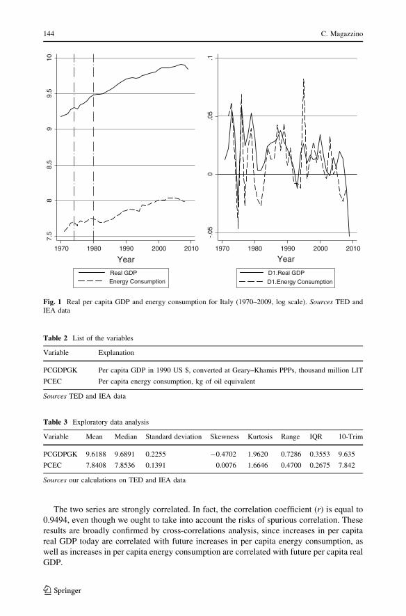
The two series are strongly correlated. In fact, the correlation coefficient (r) is equal to

0.9494, even though we ought to take into account the risks of spurious correlation. These

results are broadly confirmed by cross-correlations analysis, since increases in per capita

real GDP today are correlated with future increases in per capita energy consumption, as

well as increases in per capita energy consumption are correlated with future per capita real

GDP.

7.5

88.

59

9.5

10

1970 1980 1990 2000 2010

Year

Real GDPEnergy Consumption

-.05

0.0

5.1

1970 1980 1990 2000 2010

Year

D1.Real GDP

D1.Energy Consumption

Fig. 1 Real per capita GDP and energy consumption for Italy (1970–2009, log scale). Sources TED andIEA data

Table 2 List of the variables

Variable Explanation

PCGDPGK Per capita GDP in 1990 US $, converted at Geary–Khamis PPPs, thousand million LIT

PCEC Per capita energy consumption, kg of oil equivalent

Sources TED and IEA data

Table 3 Exploratory data analysis

Variable Mean Median Standard deviation Skewness Kurtosis Range IQR 10-Trim

PCGDPGK 9.6188 9.6891 0.2255 -0.4702 1.9620 0.7286 0.3553 9.635

PCEC 7.8408 7.8536 0.1391 0.0076 1.6646 0.4700 0.2675 7.842

Sources our calculations on TED and IEA data

144 C. Magazzino

123

4 Discussion of empirical results

As a first step, we obtained the log transformations of the time series. The inter-quartile

range (IQR) shows the absence of severe outliers in our samples. Then, we applied time

series techniques on stationarity and unit root processes, in order to check some stationarity

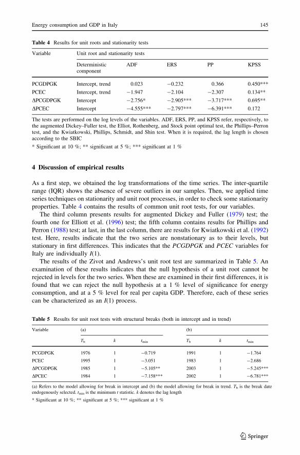
properties. Table 4 contains the results of common unit root tests, for our variables.

The third column presents results for augmented Dickey and Fuller (1979) test; the

fourth one for Elliott et al. (1996) test; the fifth column contains results for Phillips and

Perron (1988) test; at last, in the last column, there are results for Kwiatkowski et al. (1992)

test. Here, results indicate that the two series are nonstationary as to their levels, but

stationary in first differences. This indicates that the PCGDPGK and PCEC variables for

Italy are individually I(1).

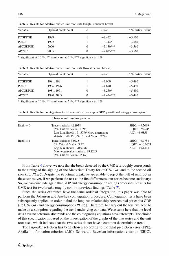
The results of the Zivot and Andrews’s unit root test are summarized in Table 5. An

examination of these results indicates that the null hypothesis of a unit root cannot be

rejected in levels for the two series. When these are examined in their first differences, it is

found that we can reject the null hypothesis at a 1 % level of significance for energy

consumption, and at a 5 % level for real per capita GDP. Therefore, each of these series

can be characterized as an I(1) process.

Table 4 Results for unit roots and stationarity tests

Variable Unit root and stationarity tests

Deterministiccomponent

ADF ERS PP KPSS

PCGDPGK Intercept, trend 0.023 -0.232 0.366 0.450***

PCEC Intercept, trend -1.947 -2.104 -2.307 0.134**

DPCGDPGK Intercept -2.756* -2.905*** -3.717*** 0.695**

DPCEC Intercept -4.555*** -2.797*** -6.391*** 0.172

The tests are performed on the log levels of the variables. ADF, ERS, PP, and KPSS refer, respectively, tothe augmented Dickey–Fuller test, the Elliot, Rothenberg, and Stock point optimal test, the Phillips–Perrontest, and the Kwiatkowski, Phillips, Schmidt, and Shin test. When it is required, the lag length is chosenaccording to the SBIC

* Significant at 10 %; ** significant at 5 %; *** significant at 1 %

Table 5 Results for unit root tests with structural breaks (both in intercept and in trend)

Variable (a) (b)

Tb k tmin Tb k tmin

PCGDPGK 1976 1 -0.719 1991 1 -1.764

PCEC 1995 1 -3.051 1983 1 -2.686

DPCGDPGK 1985 1 -5.105** 2003 1 -5.245***

DPCEC 1984 1 -7.158*** 2002 1 -6.781***

(a) Refers to the model allowing for break in intercept and (b) the model allowing for break in trend. Tb is the break date

endogenously selected. tmin is the minimum t statistic. k denotes the lag length



123

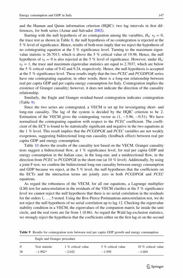
From Table 6 above, we note that the break detected by the CMR test roughly corresponds

to the timing of the signing of the Maastricht Treaty for PCGDPGK, and to the second oil

shock for PCEC. Despite the structural break, we are unable to reject the null of unit root in

these series; yet, if we perform the test at the first differences, our series become stationary:

So, we can conclude again that GDP and energy consumption are I(1) processes. Results for

CMR test for two breaks roughly confirm previous findings (Table 7).

Since the series examined have the same order of integration, this paper was able to

perform the Johansen and Juselius cointegration procedure. Cointegration tests have been

subsequently applied, in order to find the long-run relationship between real per capita GDP

(PCGDPGK) and energy consumption (PCEC). Therefore, to carry out the test, we need to

make an assumption regarding the trend underlying our data. We assume here that the level

data have no deterministic trends and the cointegrating equations have intercepts. The choice

of this specification is based on the investigation of the graphs of the two series and the unit

root tests, which indicate that the two series do not have a common deterministic trend.

The lag-order selection has been chosen according to the final prediction error (FPE),

Akaike’s information criterion (AIC), Schwarz’s Bayesian information criterion (SBIC),

Table 6 Results for additive outlier unit root tests (single structural break)

Variable Optimal break point k t stat 5 % critical value

PCGDPGK 1989 1 -2.432 -3.560

PCEC 1992 1 -3.344* -3.560

DPCGDPGK 2006 0 -5.130*** -3.560

DPCEC 2005 0 -7.025*** -3.560


Table 7 Results for additive outlier unit root tests (two structural breaks)

Variable Optimal break point k t-stat 5 % critical value

PCGDPGK 1981, 1991 1 -3.000 -5.490

PCEC 1986, 1996 1 -4.670 -5.490

DPCGDPGK 1981, 1991 0 -5.230* -5.490

DPCEC 1980, 2005 0 -7.434*** -5.490


Table 8 Results for cointegration tests between real per capita GDP growth and energy consumption

Johansen and Juselius procedure

Rank = 0 Trace statistic: 42.1938(5% Critical Value: 19.96)Log-Likelihood: 171.3796 Max.-eigenvaluestatistic: 3.0735 (5% Critical Value: 9.24)

SBIC: -9.5099HQIC: -9.6245AIC: -9.6859

Rank = 1 Trace statistic: 3.07355% Critical Value: 9.42Log-Likelihood: 190.9398Max.-eigenvalue statistic: 39.1203(5% Critical Value: 15.67)

SBIC: -9.7784HQIC: -10.0074AIC: -10.1303

146 C. Magazzino

123

and the Hannan and Quinn information criterion (HQIC): two lag intervals in first dif-

ferences, for both series (Aznar and Salvador 2002).

Starting with the null hypothesis of no cointegration among the variables, H0: r0 = 0,

the trace test as shown in Table 8, the null hypothesis of no cointegration is rejected at the

5 % level of significance. Hence, results of both tests imply that we reject the hypothesis of

no cointegrating equation at the 5 % significance level. Turning to the maximum eigen-

value statistic is 26.7013, which is above the 5 % critical value of 19.96. Hence, the null

hypothesis of r0 = 0 is also rejected at the 5 % level of significance. However, under H0:

r0 = 1, the trace and maximum eigenvalue statistics are equal to 2.7037, which are below

the 5 % critical value of 9.42 and 9.24, respectively. Hence, the null hypothesis is accepted

at the 5 % significance level. These results imply that the two PCEC and PCGDPGK series

have one cointegrating equation; in other words, there is a long-run relationship between

real per capita GDP and per capita energy consumption for Italy. Cointegration implies the

existence of Granger causality; however, it does not indicate the direction of the causality

relationship.

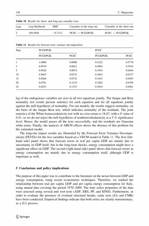
Similarly, the Engle and Granger residual-based cointegration indicates cointegration

(Table 9).

Since the two series are cointegrated, a VECM is set up for investigating short- and

long-run causality. The lag of the system is decided by the HQIC criterion to be 2.

Estimation of the VECM gives the cointegrating vector as (1, -5.96, -0.51). We have

normalized the cointegrating equation with respect to the PCEC coefficient. The coeffi-

cient of the ECT is found to be statistically significant and negative in the two equations at

the 1 % level. This result implies that the PCGDPGK and PCEC variables are not weakly

exogenous, suggesting bidirectional long-run causality (feedback effect) between real per

capita GDP and energy consumption.

Table 10 shows the results of the causality test based on the VECM. Granger causality

tests suggest a bidirectional flow, at 1 % significance level, for real per capita GDP and

energy consumption in the Italian case, in the long-run; and a unidirectional flow, in the

direction from PCEC to PCGDPGK in the short-run (at 10 % level). Additionally, by using

a joint F-test, we confirm the bidirectional long-run causality between energy consumption

and GDP because we reject, at the 5 % level, the null hypotheses that the coefficients on

the ECTs and the interaction terms are jointly zero in both PCGDPGK and PCEC

equations.

As regard the robustness of the VECM, for all our equations, a Lagrange multiplier

(LM) test for autocorrelation in the residuals of the VECM clarifies at the 5 % significance

level we cannot reject the null hypothesis that there is no serial correlation in the residuals

for the orders 1, …, 5 tested. Using the Box-Pierce Portmanteau autocorrelation test, we do

not reject the null hypothesis of no serial correlation up to lag 12. Checking the eigenvalue

stability condition in a VECM, the eigenvalues of the companion matrix lie inside the unit

circle, and the real roots are far from 1 (0.86). As regard the Wald lag-exclusion statistics,

we strongly reject the hypothesis that the coefficients either on the first lag or on the second

Table 9 Results for cointegration tests between real per capita GDP growth and energy consumption

Engle and Granger procedure

N Test statistic 1 % critical value 5 % critical value 10 % critical value

36 -1.902* -2.642 -1.950 -1.604


123

lag of the endogenous variables are zero in all two equations jointly. The Jarque and Bera

normality test results present statistics for each equation and for all equations jointly

against the null hypothesis of normality. For our models, the results suggest normality, on

the basis of the Jarque–Bera test, which indicates normality of the residuals. The joint

statistics of the White homoscedasticity test with no cross terms is 18.67, with a P value of

0.41, so we do not reject the null hypothesis of nonheteroskedasticity at a 5 % significance

level. Hence, the model passes all the tests successfully, and the residuals are Gaussian

white noise. Finally, the analysis of ARCH effects shows the absence of this problem for

the estimated model.

The long-run impact results are illustrated by the Forecast Error Variance Decompo-

sitions (FEVDs) for the two variables based on a VECM model in Table 11. The first (left-

hand side) panel shows that forecast errors in real per capita GDP are mainly due to

uncertainty in GDP itself, but in the long-term shocks, energy consumption might have a

significant effect on GDP. The second (right-hand side) panel shows that forecast errors in

energy consumption are mainly due to energy consumption itself, although GDP is

important as well.

5 Conclusions and policy implications

The purpose of this paper was to contribute to the literature on the nexus between GDP and

energy consumption, using recent econometric techniques. Therefore, we studied the

relationship between real per capita GDP and per capita energy consumption for Italy,

using annual data covering the period 1970–2009. The time series properties of the data

were assessed using several unit root tests (ADF, ERS, PP, and KPSS). Furthermore, in

order to evaluate the presence of eventual structural breaks, some tests (ZA and CMR)

have been conducted. Empirical findings indicate that both series are clearly nonstationary,

as a I(1) process.

Table 10 Results for short- and long-run causality tests

Lags Log-likelihood SBIC Causality in the long run Causality in the short run

2 189.4949 -9.7312 PCEC $ PCGDPGK PCEC ? PCGDPGK

Table 11 Results for forecast error variance decomposition

Step PCGDPGK PCEC

PCGDPGK PCEC PCGDPGK PCEC

1 1.0000 0.0000 0.4222 0.5778

3 0.9979 0.0021 0.4084 0.5916

5 0.9926 0.0074 0.3954 0.6046

10 0.9667 0.0333 0.3663 0.6337

15 0.9268 0.0732 0.3415 0.6585

20 0.8781 0.1219 0.3202 0.6798

25 0.8253 0.1747 0.3019 0.6981

148 C. Magazzino

123

Cointegration analysis revealed that there is a long-run relationship between GDP and

energy consumption. Based on a VEC model after testing for multivariate cointegration

between per capita energy use and per capita GDP, we found that energy enters signifi-

cantly into the cointegration space. The short-run dynamics of the variables show that the

flow of causality runs from energy use to GDP, and there is a long-run bidirectional causal

relationship (or feedback effect) between the two series. Yet, if there is a bidirectional

causal relationship, then economic growth may demand more energy, whereas more energy

consumption may also induce economic growth. Therefore, energy consumption and

economic growth complement each other such that radical energy conservation measures

may significantly hinder economic growth (Yang 2000; Belloumi 2009). In fact, the level

of economic activity and energy consumption mutually influence each other in that a high

level of economic growth leads to a high level of energy consumption and vice versa.

Nevertheless, this sort of dependence indicates the need to diversify energy sources,

inasmuch as the country must weigh the need for sustainable economic growth against the

environmental costs associated with excessive energy consumption.

Furthermore, the short-run causality findings seem to confirm the ‘‘growth hypothesis’’

in the case of Italy, i.e., that implementation of energy conservation policies would not

adversely affect output, but on the contrary would steer economic growth. It follows that

the cuts in energy consumption due to the enactment of the ‘‘Kyoto Protocol’’ will actually

harm the Italian economy.

In brief, the economy of Italy seems to be declining as a consequence of the increasing

cost (or—equivalently—declining energy returns) of primary energy sources, mainly

natural gas and crude oil. If such is the case, decline is irreversible. The only possibility to

avoid this outcome is to decouple the economy from nonrenewable resources, generating

energy using renewable ones.

6 Suggestions for future researches

Further analysis may be conducted studying the nexus between different sources of energy

and GDP in Italy (Magazzino 2012). This could well contribute to the debate on Italy’s

return to nuclear power. Our conclusions for Italy may be relevant for a number of

countries that have to go through a similar development path of increased pressure on

already scarce energy resources. Moreover, a lot of researcher recently explored the

dynamic relationship between emissions, economic growth, and energy consumption.

Thus, to achieve sustainable economic growth, it might be explored the dynamic rela-

tionship between emissions, economic growth, and energy consumption for Italy. Finally,

future research could include variables such as physical capital, human capital, and labor to

estimate the long-run elasticities, following the methods of Mankiw et al. (1992).

References

Abosedra, S., & Baghestani, H. (1989). New evidence on the causal relationship between United Statesenergy consumption and gross national product. Journal of Energy Development, 14, 285–292.

Akarca, A. T., & Long, T. V. (1980). On the relationship between energy and GNP: A reexamination.Journal of Energy Development, 5, 326–331.

Altinay, G., & Karagol, E. (2004). Structural break, unit root, and the causality between energy consumptionand GDP in Turkey. Energy Economics, 26(6), 985–994.


123

Andrews, D., & Zivot, E. (1992). Further evidence on the Great Crash, the oil price shock, and the unit-roothypothesis. Journal of Business and Economic Statistics, 10, 251–270.

Ang, J. B. (2007). CO2 emissions, energy consumption, and output in France. Energy Policy, 35,4772–4778.

Ang, J. B. (2008). Economic development, pollutant emissions and energy consumption in Malaysia.Journal of Policy Modeling, 30, 271–278.

Apergis, N., & Payne, J. E. (2009). Energy consumption and economic growth in Central America: Evi-dence from a panel cointegration and error correction model. Energy Economics, 31, 211–216.

Aqeel, A., & Butt, M. S. (2001). The relationship between energy consumption and economic growth inPakistan. Asia Pacific Development Journal, 8(2), 101–110.

Asafu-Adjaye, J. (2000). The relationship between energy consumption, energy prices and economicgrowth: Time series evidence from Asian developing countries. Energy Economics, 22, 615–625.

Aznar, A., & Salvador, M. (2002). Selecting the rank of the cointegration space and the form of the interceptusing an information criterion. Econometric Theory, 18, 926–947.

Belloumi, M. (2009). Energy consumption and GDP in Tunisia: Cointegration and causality analysis.Energy Policy, 37(7), 2745–2753.

Borozan, D. (2013). Exploring the relationship between energy consumption and GDP: Evidence fromCroatia. Energy Policy, 59, 373–381.

Campbell, J. Y., & Perron, P. (1991). Pitfalls and opportunities: What macroeconomists should know aboutunit roots and cointegration, NBER macroeconomics annual. Cambridge, MA: MIT Press.

Campo, J., & Sarmiento, V. (2013). The relationship between energy consumption and GDP: Evidence froma panel of 10 Latin American countries. Latin American Journal of Economics, 50(2), 233–255.

Cheng, B. S. (1995). An investigation of cointegration and causality between energy consumption andeconomic growth. Journal of Energy Development, 21, 73–84.

Cheng, B. S. (1997). Energy consumption and economic growth in Brazil, Mexico and Venezuela: A timeseries analysis. Applied Economics Letters, 4(11), 671–674.

Cheng, B. S. (1999). Causality between energy consumption and economic growth in India: An applicationof cointegration and error-correction modeling. Indian Economic Review, 34, 39–49.

Cheng, B. S., & Lai, T. W. (1997). An investigation of co-integration and causality between energyconsumption and economic activity in Taiwan. Energy Economics, 19(4), 435–444.

Chen, S. T., Kuo, H. I., Chen, C. C. (2007). The relationship between GDP and electricity consumption in 10Asian countries, Energy Policy, 35, 2611–2621.

Chiou-Wei, S. Z., Chen, C.-F., & Zhu, Z. (2008). Economic growth and energy consumption revisited—Evidence from linear and nonlinear Granger causality. Energy Economics, 30(6), 3063–3076.

Chontanawat, J., Hunt, L. C., & Pierse, R. (2006). Causality between energy consumption and GDP:Evidence from 30 OECD and 78 Non-OECD Countries, SEEDS Working Paper, 113.

Chontanawat, J., Hunt, L. C., & Pierse, R. (2008). Does energy consumption cause economic growth?Evidence from a systematic study of over 100 countries. Journal of Policy Modeling, 30, 209–220.

Clemente, J., Montanes, A., & Reyes, M. (1998). Testing for a unit root in variables with a double change inthe mean. Economics Letters, 59, 175–182.

Climent, F., & Pardo, A. (2007). Decoupling factors on the energy-output linkage: The Spanish case. EnergyPolicy, 35, 522–528.

Dagum, E. B. (2002). Analisi delle serie storiche: Modellistica, previsione e scomposizione. Milan:Springer.

Dakhlaoui, D., Amiri, K., & Talbi, B. (2012). Climate components and economic growth in Tunisia:Cointegration and causality analysis. Australian Journal of Basic and Applied Sciences, 6(9), 171–177.

Dickey, D. A., & Fuller, W. A. (1979). Distribution of the estimators for autoregressive time series with aunit root. Journal of the American Statistical Association, 74, 427–431.

Elliott, G., Rothenberg, T. J., & Stock, J. H. (1996). Efficient tests for an autoregressive unit root. Eco-nometrica, 64, 813–836.

Enders, W. (2003). Applied econometric time series. Chichester: Wiley.Erdal, G., Erdal, H., & Esengun, K. (2008). The causality between energy consumption and economic

growth in Turkey. Energy Policy, 36(10), 3838–3842.Erol, U., & Yu, E. S. H. (1987). On the causal relationship between energy and income for industrialized

countries. Journal of Energy Development, 13, 113–122.Fatai, K., Oxley, L., & Scrimgeour, F., (2002). Energy consumption and employment in New Zealand:

Searching for causality. Paper presented at NZAE conference. Wellington, 26–28 June 2002.Franses, P. H. (2002). Time series models for business and economic forecasting. Cambridge: Cambridge

University Press.

150 C. Magazzino

123

Ghali, K. H., & El-Sakka, M. I. T. (2004). Energy use and output growth in Canada: A multivariatecointegration analysis. Energy Economics, 26, 225–238.

Glasure, Y. U. (2002). Energy and national income in Korea: Further evidence on the role of omittedvariables. Energy Economics, 24, 355–365.

Glasure, Y. U., & Lee, A. (1997). Cointegration, error correction and the relationship between GDP andenergy: The case of South Korea and Singapore. Resource and Energy Economics, 20, 17–25.

Granger, C. W. J., & Newbold, P. (1974). Spurious regressions in econometrics. Journal of Econometrics, 2,111–120.

Halicioglu, F. (2009). An econometric study of CO2 emissions, energy consumption, income and foreigntrade in Turkey. Energy Policy, 37, 1156–1164.

Hamilton, J. D. (1994). Time series analysis. Princeton: Princeton University Press.Ho, C-Y., Siu, K. W. (2007). A dynamic equilibrium of electricity consumption and GDP in Hong Kong:

and empirical investigation. Energy Policy, 35(4), 2507–2513.Hondroyiannis, G., Lolos, S., & Papapetrou, E. (2002). Energy consumption and economic growth:

Assessing the evidence from Greece. Energy Economics, 24, 319–336.Hwang, D., & Gum, B. (1991). The causal relationship between energy and GNP: The case of Taiwan.

Journal of Energy Development, 16, 219–226.Iwayemi, A. (1998). Energy sector development in Africa. African development report.Jobert, T., & Karanfil, F. (2007). Sectoral energy consumption by source and economic growth in Turkey.

Energy Policy, 35, 5447–5456.Johansen, S. (1988). Statistical analysis of cointegrating vector. Journal of Economic Dynamics and Con-

trol, 12(2–3), 231–255.Johansen, S., & Juselius, K. (1990). Maximum likelihood estimation and inference on cointegration with

applications to the demand for money. Oxford Bulletin of Economics and Statistics, 52(2), 169–210.Karanfil, F. (2008). Energy consumption and economic growth revisited: Does the size of unrecorded

economy matter? Energy Policy, 36(8), 3029–3035.Kebede, E., Kagochi, J., & Jolly, C. M. (2010). Energy consumption and economic development in Sub-

Saharan Africa. Energy Economics, 32, 532–537.Kraft, J., & Kraft, A. (1978). On the relationship between energy and GNP. Journal of Energy and

Development, 3, 401–403.Kwiatkowski, D., Phillips, P. C. B., Schmidt, P., & Shin, Y. (1992). Testing the null hypothesis of sta-

tionarity against the alternative of a unit root: How sure are we that economic time series have a unitroot? Journal of Econometrics, 54, 159–178.

Lee, C. C. (2005). Energy consumption and GDP in developing countries: A cointegrated panel analysis.Energy Economics, 27, 415–427.

Lee, C. C. (2006). The causality relationship between energy consumption and GDP in G-11 countriesrevisited. Energy Policy, 34, 1086–1093.

Lee, C. C., & Chang, C. P. (2005). Structural breaks, energy consumption, and economic growth revisitedevidence from Taiwan. Energy Economics, 27, 857–872.

Lee, C. C., & Chang, C. P. (2007). Energy consumption and GDP revisited: A panel analysis of developedand developing countries. Energy Economics, 29, 1206–1223.

Lise, W., & Van Montfort, K. (2007). Energy consumption and GDP in Turkey: Is there a co-integrationrelationship? Energy Economics, 29, 1166–1178.

Lutkepohl, (2005). New introduction to multiple time series analysis. Milan: Springer.Magazzino, C. (2012). On the relationship between disaggregated energy production and GDP in Italy.

Energy & Environment, 23(8), 1191–1207.Magazzino, C. (2014a). Electricity Demand, GDP and employment: Evidence from Italy. Frontiers in

Energy, 8, 1, 31–40.Magazzino, C. (2014b). The relationship between CO2 emissions, energy consumption and economic

growth in Italy. International Journal of Sustainable Energy (forthcoming).Mahadevan, R., & Asafu-Adjaye, J. (2007). Energy consumption, economic growth and prices: A reas-

sessment using panel VECM for developed and developing countries. Energy Policy, 35(4),2481–2490.

Mankiw, N. G., Romer, D., & Weil, D. N. (1992). A contribution to the empirics of economic growth. TheQuarterly Journal of Economics, 107(2), 407–437.

Masih, A. M. M., & Masih, R. (1996). Energy consumption and real income temporal causality, results for amulti-country study based on cointegration and error-correction techniques. Energy Economics, 18,165–183.


123

Masih, A. M. M., & Masih, R. (1997). On temporal causal relationship between energy consumption, realincome and prices; some new evidence from Asian energy dependent NICs based on a multivariatecointegration/vector error correction approach. Journal of Policy Modeling, 19(4), 417–440.

Mehrara, M. (2007). Energy consumption and economic growth: The case of oil exporting countries. EnergyPolicy, 35(5), 2939–2945.

Mishra, V., Smyth, R., & Sharma, S. (2009). The energy-GDP nexus: Evidence from a panel of PacificIsland countries. Resource and Energy Economics, 31(3), 210–220.

Narayan, P. K., & Smyth, R. (2008). Energy consumption and real GDP in G7 countries: New evidence frompanel cointegration with structural breaks. Energy Economics, 30, 2331–2341.

Nelson, C., & Plosser, C. (1982). Trends and random walks in macroeconomics time series: Some evidenceand implications. Journal of Monetary Economics, 10, 139–162.

Odhiambo, N. M. (2009). Energy consumption and economic growth nexus in Tanzania: An ARDL boundstesting approach. Energy Policy, 37(2), 617–622.

Oh, W., & Lee, K. (2004a). Causal relationship between energy consumption and GDP: The case of Korea1970–1999. Energy Economics, 26(1), 51–59.

Oh, W., & Lee, K. (2004b). Energy consumption and economic growth in Korea: Testing the causalityrelation. Journal of Policy Modeling, 26, 973–981.

Ozturk, I. (2010). A literature survey on energy-growth nexus. Energy Policy, 38, 340–349.Paul, S., & Bhattacharya, R. N. (2004). Causality between energy consumption and economic growth in

India: A note on conflicting results. Energy Economics, 26(6), 977–983.Payne, J. E. (2009). On the dynamics of energy consumption and output in the US. Applied Energy, 86(4),

575–577.Pereira, A. M., & Pereira, R. M. M. (2010). Is fuel-switching a no-regrets environmental policy? VAR

evidence on carbon dioxide emissions, energy consumption and economic performance in Portugal.Energy Economics, 32, 227–242.

Perron, P. (1989). The great crash, the oil price shock, and the unit root hypothesis. Econometrica, 57,1361–1401.

Perron, P. (1990). Testing for a unit root in a time series with a changing mean. Journal of Business andEconomic Statistics, 8, 153–162.

Phillips, P. C. B. (1986). Understanding spurious regression in econometrics. Journal of Econometrics,33(3), 311–340.

Phillips, P. C. B., & Perron, P. (1988). Testing for a unit root in time series regression. Biometrika, 75,335–346.

Ranci, P. (Ed.). (2011). Economia dell’energia. Bologna: il Mulino.Soytas, U., & Sari, R. (2003). Energy consumption and GDP: Causality relationship in G-7 countries and

emerging markets. Energy Economics, 25, 33–37.Soytas, U., & Sari, R. (2006). Energy consumption and income in G7 countries. Journal of Policy Modeling,

28, 739–750.Soytas, U., & Sari, R. (2009). Energy consumption, economic growth, and carbon emissions: Challenges

faced by an EU candidate member. Ecological Economics, 68(6), 1667–1675.Soytas, U., Sari, R., & Ewing, B. T. (2007). Energy consumption, income, and carbon emissions in the

United States. Ecological Economics, 62(3–4), 482–489.Soytas, U., Sarı, R., & Ozdemir, O. (2001). Energy consumption and GDP relation in Turkey: A cointe-

gration and vector error correction analysis. Economies and Business in Transition, 838–844.Stern, D. I. (1993). Energy and economic growth in the USA. A multivariate approach, Energy Economics,

15, 137–150.Stern, D. I. (2000). A multivariate cointegration analysis of the role of energy in the US macroeconomy.

Energy Economics, 22, 267–283.Stock, J., & Watson, M. (1988). Testing for common trends. Journal of the American Statistical Association,

83, 1097–1107.Thoma, M. (2004). Electrical energy usage over the business cycle. Energy Economics, 26, 463–485.Tsani, S. Z. (2010). Energy consumption and economic growth: A causality analysis for Greece. Energy

Economics, 32, 582–590.Tugcu, C. C., Ozturk, I., & Aslan, A. (2012). Renewable and non-renewable energy consumption and

economic growth relationship revisited: Evidence from G7 countries. Energy Economics, 34(6),1942–1950.

Wolde-Rufael, Y. (2004). Disaggregated industrial energy consumption and GDP: The case of Shanghai,1952–1999. Energy Economics, 26, 69–75.

Wolde-Rufael, Y. (2009). Energy consumption and economic growth: The experience of African countriesrevisited. Energy Economics, 31(2), 217–224.

152 C. Magazzino

123

Yang, H. Y. (2000). A note on the causal relationship between energy and GDP in Taiwan. EnergyEconomics, 22(3), 309–317.

Yu, E. S. H., & Choi, J. Y. (1985). The causal relationship between energy and GNP: An internationalcomparison. Journal of Energy and Development, 10, 249–272.

Yu, E. S. H., & Hwang, B. K. (1984). The relationship between energy and GNP: Further results. EnergyEconomics, 6, 186–190.

Yu, E. S. H., & Jin, J. C. (1992). Cointegration tests of energy consumption, income, and employment.Resources and Energy, 14, 259–266.

Yuan, J.-H., Kang, J.-G., Zhao, C.-H., & Hu, Z.-G. (2008). Energy consumption and economic growth:Evidence from China at both aggregated and disaggregated levels. Energy Economics, 30, 3077–3094.

Zachariadis, T. (2007). Exploring the relationship between energy use and economic growth with bivariatemodels: New evidence from G-7 countries. Energy Economics, 29, 1233–1253.

Zamani, M. (2007). Energy consumption and economic activities in Iran. Energy Economics, 29,1135–1140.

Zhang, X.-P., & Cheng, X.-M. (2009). Energy consumption, carbon emissions, and economic growth inChina. Ecological Economics, 68, 2706–2712.


123

Energy consumption and GDP in Italy: cointegration and causality analysis

Documents

Transcript of Energy consumption and GDP in Italy: cointegration and causality analysis