OXFORD BULLETIN OF ECONOMICS AND STATISTICS, 54, 3 (1992) 0305-9049 $3.00 .

THE POWER OF COINTEGRATION TESTS

Jeroen J. M. Kremers, Neil R. Ericsson and Juan J. Dolado I

1. INTRODUCTION

Contrasting inferences about the presence of cointegration often appear in empirical investigations. For example, in applying the cornmonly used 'two­step' procedure proposed by Engle and Granger (1987), the Dickey-Fuller unit-root test may only marginally reject the null hypothesis of no cointegra­tion, if it rejects at all. By contrast, the coefficient on the error-correction term in the corresponding dynamic model of the same data may be 'highly statistically significant', strongly supporting cointegration; cf. Kremers (1989), Hendry and Ericsson (1991a), and Campos and Ericsson (1988). Both procedures are tests of cointegration, so why should there be such a contrast? A plausible explanation centers on an implicit common factor restriction imposed when using the Dickey-Fuller statistic to test for cointe­gration. If that restriction is invalid, the Dickey-Fuller test remains consist­ent, but loses power relative to cointegration tests that do not impose a common factor restriction, such as those based upon the estimated error­correction coefficient.

This paper examines the asymptotic and finite sample properties of the two procedures for a simple, single-lag, bivariate process. Even with more lags and more variables, the reason for the low power of the Dickey-Fuller test remains. The error-correction-based test is preferable because it uses available information more efficiently than the Dickey-Fuller test.

Section II describes the process of interest and derives the relationship between the error-correction mechanism and the equation from which the Dickey-Fuller statistic is calculated. Section III presents the asymptotic distribution of each test statistic under the null hypothesis of no cointegra-

I This paper represents the views of the authors and should not be interpreted as reflecting those of the Dutch Ministry of Finance, the Board of Govemors of the Federal Reserve System, the Bank of Spain, or other members of their staff. This paper was prepared in part while the second and third authors were visiting INSEE and CEPREMAP, who we thank for generous hospitality. We are grateful to Javier Andrés, Anindya Banerjee, Julia Campos, Christian Gourieroux, David Hendry, S0ren Johansen, Augustín Maravall, A1ain Monfort, Mark Salmon, Jim Stock, and Hong-Anh Tran for helpful discussions, and to Lisa Barrow and Rafael Domenech for research assistance. AH numerical results were obtained using PC-NAIVE ~._ ... ~. PC-GIVE Version 6.01; cf. Hendry and Neale (1990) and Hendry (1989). /.~., 00

325 1

326 BULLETIN

tion, while Section IV gives the corresponding asymptotic distributions under the altemative hypothesis of cointegration, using fixed and 'near non­cointegrated' altematives. Section V generalizes the results for testing in multivariate, multiple-Iag systems. Section VI interprets sorne Monte Cario finite sample evidence in light of the asymptotic formulae. Section VII empirically illustrates the two testing procedures with Hendry and Ericsson's (1991 b) quarterly data on UK narrow money demando Derivations of all new results appear in the Appendix.

n. A SIMPLE BIVARIATE PROCESS

Using a simple dynamic bivariate process, this paper focuses on the relative merits of the two-step Engle-Granger and single-step dynamic-model procedures for testing for the existence of cointegration. See Engle and Granger (1987) on the former and Banerjee, Dolado, Hendry and Smith (1986) in ter alia on the latter. The former is characterized by a Dickey-Fuller (DF) statistic used to test for the existence of a unit root in the residuals of a static cointegrating regression. The latter is based upon the t-ratio of the coefficient on the error-correction term in a dynamic model reparameterized as an error-correction mechanism (ECM), noting that cointegration implies and is implied by an ECM. This t-ratio is denoted the ECM statistic. This section describes the data generation process (DGP) and derives the analytical relationship between the ECM and the equation for the DF statistic.

The bivariate process- considered is one of the simplest imaginable, and has been used elsewhere for expository purposes; cf. Davidson, Hendry, Srba and Yeo (1978) and Banerjee, Dolado, Hendry and Smith (1986). It is a linear first-order vector autoregression with normal disturbances, at least one unít root, and Granger-causality in only one direction. For expositional convenience, this DGP is written as a conditional ECM (1) and a m~rginal unít-root process (2):

~y¡ =a~z¡+ b(y -zL-, + e¡ ~z¡=u¡

(1) t= 1, ... , T, (2)

where ~ is the first-difference operator 1 - L, L is the lag operator, and T is the sample size. The variables y¡ and Z¡ are integrated of order one [denoted I( 1)] and are possibly cointegrated. For y = In Y and z = In Z, a is the short­run elasticity of Y with respect to Z. The parameter b is the error-correction coefficient in the conditional model of y¡, given lagged y and current and lagged z; and e¡ and U¡ are the disturbances in this conditional/marginal fac­torization. Without los s of generality, the cointegrating vector for (YI z¡)' is (1, - 1) if YI and z¡ are cointegrated.

For simplicity, the (hypothesized) cointegrating vector is assumed known. Such a priori knowledge of the cointegrating vector anses frequently in

THE POWER OF COINTEGRATION TESTS 327

economic models of long-run behavior, as in modeling (logs of) consumers' expenditure and disposable income, wages and prices, money and income, or the exchange rate and foreign and domes tic price levels.2 AIso, Z¡ is assumed weakly exogenous for the parameters in the conditional model ( 1); see Engle, Hendry and Richard (1983) and Johansen (1992a).

As Section V shows, the logical issues arising from cornmon factor restric­tions apply to processes more general than (1 )-( 2). Specifically, the cointe­grating vector or vectors may be estimated and may enter more than one equation (e.g., no weak exogeneity); and a constant term, seasonal dummies, additional variables, and additional lags may be included. However, sorne statistics' distributions are more complicated with such generalizations, so we focus on this bivariate case.

The parameter space is restricted to {O~a~l, -l<b~O}. In many empirical studies, a'" 0.5 and b'" - 0.1, with a~ > a;. That is, the short-run elasticity (a) is smaller than the long-run elasticity (unity), adjustment to remaining disequilibria is slow, and the innovation error variance for the regressor process is larger than that of the conditional ECM.

The variables y¡ and z¡ are cointegrated or not, depending upon whether b < O or b = O. Thus, tests of cointegration rely upon sorne estimate of b. In the ECM approach, equation (1) itself is estimated by OLS (denoted by a circumflex A):

~y¡ = á~z¡ + bw¡_, + tI' where the putative disequilibrium is:

(3)

(4)

The t-ratio based upon b is the ECM statistic, denoted tECM ' It is used to test the null hypothesis that b = O, i.e., that y and z are not cointegrated with a cointegrating vector (1, - 1).

The DF statistic derives from a different regression, so it is helpful to establish the relationship between the DF regression equation and the ECM in ( 1). Specifically, subtract ~z¡ from both sides of (1) and re-arrange:

~(y-zL=b(y-zL_, +[(a-1)~z¡+eJ (5)

N oting (4), equation (5) may be rewritten as:

(6)

where the disturbance e¡ is: e¡=(a-1)~z¡+e¡. (7)

2See Davidson, Hendry, Srba and Yeo (1978), Hendry, Muellbauer and Murphy (1990), Sargan (1964), Nymoen (1992), Hendry and Ericsson (1991a, 1991b), and Johansen and Juselius (1990a, 1990b) ínter alía.

2

328 BULLETIN

OLS estimation of (6) (denoted by a tilde ~) generates:

dw,=bw,_1 +el· (8)

The t~ratio based upon b is the DF statistic, denoted tOF here [i in Dickey and Fuller, 1979]. This t~ratio is also used to test whether or not YI and ZI are cointegrated with cointegrating vector (1, -1). See Dickey and Fuller (1979, 1981) and Engle and Granger ( 1987).

In contrast to the estimated ECM in (3), the estimated DF equation (8) ignores potential information contained in dz,. Equivalently, (6) imposes the restriction that a equals unity. That is, the short~run elasticity (a) equals the long~run elasticity (unity). More generally, (6) imposes a common factor, as follows from rewriting (4) and (6):

(9)

or

[1- (1 + b) L] YI = [1- (1 + b) L] ZI + e" (10)

where [1- (1 + b) L] is the factor common to YI and ZI in (10).3 The transformation of (1) to (6), (9), and (10) provides several insights.

First, (1), (6), (9), and (10) are equivalent representations, given the rela­tionship between the errors El and el in (7); but the two errors are not equal unless a = 1 or dZ, = O. Second, and relatedly, the common factor restriction in ( 10) [and so in (6) and (9)] is invalid unless a = 1, noting that:

[l-(l+b)L]y,=[a-(a+b)L]z,+E" (11) from (1). Interestingly, even if the common factor restriction is invalid, el remains white noise for this DGP. Nonetheless, el is not an innovation with respect to current and lagged Z and lagged y; cf. Granger (1983) and Hendry and Richard (1982) on the distinction between white noise and innovations. Since empirically estimated short- and long-run elasticities often differ markedly (as noted aboye), imposing their equality in the DF statistic is rather arbitrary. Third, (9) motivates the use of unit-root statistics in testing for cointegration. If wl has a unit root, then wl is non-stationary, b = O, and YI and Z I are not cointegrated with the cointegrating vector (1, - 1). Conversely, if WI

has its root inside the unit circle, then wl is stationary, b < O, and YI and ZI are cointegrated.

III. DISTRIBUTION OF THE STATISTICS UNDER THE NULL HYPOTHESIS (NO COINTEGRATION)

The null hypothesis is no cointegration: that is, b= O in (1)-(2). Because W I _ 1 [in (3) and (8)] is not stationary under this hypothesis, distributional results

3 See Hendry and Mizon (1978) and Sargan (1964, 1980) on commo~ factors.

THE POWER OF COINTEGRATION TESTS 329

from 'standard' asymptotic theory do not apply. This section describes the asymptotic distributions of the DF and ECM statistics under that null hypothesis, and obtains a normal approximation to the distribution of the ECM t~ratio when a ~ 1.

For expositional convenience, we adopt certain notational conventions conceming Brownian motion (or Wiener) processes. Consider a normal, independently and identically distributed variable r¡ l' t = 1, ... , T: that is, r¡,-1N(0, a~). In this paper, r¡1 is usually either el' El' or UI. Define BT. '1(r) as the partial sum ~Itrlr¡'/J( Ta~), where r lies in [0,1], and [Tr] is the integer part of Tr. As discussed in Phillips (1987b), BT.'1(r) converges weakly to a standardized Wiener process, denoted B'1(r). Frequently, the argument r is suppressed, as is the range of integration over r, when that range is lO, 1J. Thus, integrals such as fóB'1(r)2 dr are written as f B~. The symbol ,~' denotes weak convergence of the associated probability measures as the sample size T -+ oo. See Banerjee, Dolado, Galbraith and Hendry ( 1992) for a detailed discussion of Wiener processes.

The DF statistic [from (8)] is:

tOF = bjese(b)

= [(~W¡_I)-I(~W'_ldW/)]IJ[ü; '(~W¡_I)-I] = (~W¡_I)-I/2(~WI_1 el)jüe , (12)

where ese(') is the estimated standard error of its argument, ü; is the estimated residual variance in (8), and all summations ~ are from 1 to T unless otherwise noted. Dickey and Fuller ( 1979) show that:

(13)

under the null hypothesis. Dickey lin Fuller, 1976, p. 373] tabulates by Monte Cario the finite sample distribution for tOF, from whichcritical values may be taken for constructing a unit-root test.

The DF statistic has several important properties. First, its distribution is skewed to the left, and it has a negative median. In part because of these characteristics, the use of (negative) one-sided normal critical values may result in over-rejection under the null hypothesis. Second, the distribution of the DF statistic is invariant to au , a t , and a, even in finite samples; cf. (12).

Banerjee, Dolado, Hendry and Smith (1986, Theorem 4) derive the asymptotic distribution of the t-ratio on b in the ECM (3). Our Appendix corrects their formula and obtains a simpler normal approximation for a ~ 1. Since ~dzlwl_l.is Op( T) and E(UIE/)=O, the ECM t-ratio is:

tECM = bjese(b)

(14)

where a~ is the estimated residual variance in (3), and Mann and Wald's (1943) order notation is used. Ignoring the term of Op( T -1/2), (14) is identical

3

330 BULLETIN

to the DF statistic in (12), except that el appears rather than el' Using properties of independent Brownian motion, the lirniting distribution of tECM

is:

tECM ~ (f Be dB,)!J(f B;)

(a-1)fB"dB,+s-lfB,dB, ~ 2 2 1 2 2' J[(a-1)fB,,+2(a-1)s fB"B,+s fB,]

where s is the ratio aja, (assumed strictly positive).

(15)

As will be discussed below, the distribution of tECM depends on the relative importance of the two terms comprising e, in (7), which are (a - 1) I:!z, and e,. Specifically, it is useful to define a 'signal-to-noise' ratio:

q = -(a-1) s, (16)

where q2 is the variance of (a - 1) I:!ZI relative to that of e l' Equally, q2 is g¡ 2/( 1 - g¡ 2), where g¡ 2 is the population R 2 with b = O for I:! w, regressed on wl _ 1 and I:!ZI' as in (28) below.

The asymptotic distribution of the ECM statistic has several unusual properties. First, because I:!z, is observed and is conditioned upon in estimat­ing (3), q measures the amount of information present on the invalidity of the common factor restriction (for a given T). Second, and relatedly, when a = 1 (and so q = O), (15) simplifies to the D F distribution (13), noting that el = el (and hence Be = B,) for a = 1. Third, for a #- 1, ( 15) can be reparameterized in terms of q exclusively, rather than a and s separately:

tECM ~ I 2 - 1 2f 2]' .¡[fB,,-2q fB"B,+q B, (17)

The asymptotic distribution of tECM is sensitive to a and s only insofar as they enter q.

Fourth, for large q, (17) is approximately a standardized normal distribu­tion:

(18)

This second approximation is 'small-a' in nature or, equivalently, assumes the signal-to-noise ratio for (3) to be large; cf. Kadane (1970, 1971 ).4 As q varies from small to large, the asymptotic distribution of tECM shifts from the DF distribution to the normal distribution. To obtain ( 18), note that ( 17) is:

(19)

4 Complementary interpretations exist. From (1) and (2) with b = O and a ~ O, YI and ZI are virtuaIly identicaI series for large q (a constant term and factor of proportic:mality aside! ~eca~se the variance of aL!.ZI is large relative to that of f l . Thus, YI and ZI appear comtegrated, gIVmg .n~e to 'standard' inferentiaI procedures for b. This reasoning does not apply to the DF staUstIc because it is invariant to the variance of el'

THE POWER OF COINTEGRATION TESTS 331

Since Bu and B, are independent Brownian motions, the ratio in (19) is normally distributed; see Phillips and Park (1988).

Thus, when the common factor restriction in (9) is invalid and I:!ZI con­tributes substantively to the determination of I:! YI' the t-ratio on the error­correction term in (3) is approximately normal, even when the error-correction coefficient is zero and so YI and ZI are not cointegrated. That simplifies conducting inference with tECM when q is large.5 The distribution of tOF is independent of a, au' and a, (and thus of s and q), even in finite samples, so no parallel approximation exists for tOFo

To summarize, in so far as distributions under the null are concerned, tECM has a distinct advantage over tOF when q is known to be large because of the former's approximate normality under that condition. The next section considers distributions under the alternative hypothesis of cointegration, and so the issue of power.

IV. DISTRIBUTION OF THE STATISTICS UNDER THE ALTERNATIVE

HYPOTHESIS (COINTEGRATION)

The alternative hypothesis is cointegration: namely, b < O in (1 H 2). This section examines the asymptotic distributions of the DF and ECM statistics under both fixed and local alterna ti ves. A priori, the distributions derived undér either alternative could approximate the underlying finite sample distributions well, so both altematives are of interest. Under a fixed alterna­tive, W,_ 1 in (3) and (8) is stationary, so distributional results foUow from con­ventional central limit theorems. Under a local alternative, the non-conventional asymptotic theory developed by Phillips (1988) for near­integrated series can be applied.

Section 4.1 compares the asymptotic distributions of the DF and ECM statistics under a fixed alterna ti ve; Section 4.2 compares them under a local alternative. When a = 1, the two statistics are asymptotically equivalent. When a #- 1, the ECM test can be arbitrarily more powerful than the DF test.

4.1. Distributions under a Fixed Alternative

Under a fixed altemative, this subsection analyzes the components of the DF and ECM statistics, from which the properties of the statistics themselves can be compared.

For the DF statistic, the numerator is:

b= (~W~-'-l)-l(~WI_lI:!W,) = b +(~W~_l)-l(~W'_l eJ, (20)

51f no information is available on the magnitude of q, then it appears advisable to use the DF criticaI values for the ECM statistic because they are larger in absolute value than the critical vaIues for the normal. This choice follows from the definition of statistical size involving the supremum over the appropriate parameter space, here, being over the range of a and S.

4

332 BULLETIN

from which it follows that:

TI/2 '(b - b)=> N(O, a;/a~),

where a~ = a;/[ 1 - (1 + b)2]. The denominator of the DF statistic is:

ese(b)= T-I/2ae/aw + Op( T-I).

For the ECM statistic, the numerator is:

0= b +(l:W~_I¡-I(l:Wt_1 Et)+ Op(T -1),

which implies:

TI/2 '(0 - b)=> N(O, a;/a~).

The denominator of the ECM statistic is:

ese(o)= T-I/2 a.law + Op( T-I).

(21)

(22)

(23)

(24)

(25)

Combining these results obtains a relationship between the two statistics:

tECM o/ese(o) tDF b /ese( b)

= a./a, + Op( T-I/2). (26)

That is, the ECM statistic isapproximately ae/a, times the DF statistic. That factor of proportionality is at least unity,and in general is greater thanunity, noting that:

a;/a; =[(a-1)2a;' + aWa;

=(1 + q2)~ 1 (27)

from (7). The degree ofinequality depends upon q. Relative power is likewise affected, as illustrated in Section VI via Monte Cario.

Intuition for the differences between the statistics is as follows. The ECM regression conditions on both 6.z t and W t - l' whereas the DF regression conditions on only wt - I , thereby losing potentially valuable information from 6.zt • Rewriting (5) helps clarify:

(28)

where, as an extreme example, Et "" O, a oF 1, and Var(6.zt) is 'substantial' (and so q is large). The ECM (28) has a near perfect fit, a and b are estimated with near exact precision, and the ECM t-ratio for b is (arbitrarily) large. However, the DF statistic is invariant to the variance of et (and so to the values of a and s), and the distribution of the DF statistic depends upon only b and T. For a suitably small (but nonzero) value of b and a given T, the DF statistic has Httle power (e.g., approximating its size) while the ECM statistic has power close to unity. This arises because the DF stat~stic ignores valuable information about 6.zt that is present in et' Nevertheless, both statistics are

THE POWER OF COINTEGRATION TESTS 333

Op( TI /2) under a fixed alternative, so motivating a local alternative to obtain statistics of O p( 1 ).

4.2. Distributions under a Local Alternative

To formalize the previous intuition, we apply Phillips's (1988) noncentral distribution theory to analyze the local asymptotic properties of the test statistics. The DGP is (1 )-(2) with the local alternative:

b = ec/T - 1 "" c /T, (29)

where c is a negative fixed scalar. The local alternative (29) parallels the usual Pitman-type local alterna ti ve, except that, in order to obtain statistics of O p( 1), (29) differs from the null by O p( T - 1 ), rather than by O p( T - 1/2).

To proceed, we follow Phillips (198 7b) and use the diffusion process:

K~(r)=f" ér-j)c dB~(j) ()

(30)

where K~(r) is an implicit function of c. If c=O, then K~(r) is B~(r). As with B~, the argument r and the limits of integration are dropped if no ambiguity arises from doing so.

Under the local alternative (29), the DF statistic is distributed as:

(31)

see Phillips (198 7b, p. 541; 1988, (26)). As shown in the Appendix, the ECM statistic is distributed as:

t =>C(1+q2)1/2(fK2)1/2+ (a-1)fKll dB,+s-lfK,dB, ECM e J[(a-1)2fK~+2(a-1)s IfKIIK,+s 2fK;]'

(32)

Properties of the asymptotic distributiorts in (31) and (32) are closely related to results under the null hypothesis. First, when c=O, (32) simplifies to the distribution under the null, (17). Likewise, the asymptotic distribution (31) for the DF statistic reduces to (13) under the null. Second, when a= 1, (32) simplifies to the DF distribution (31). Third, for aoF 1, (32) can be reparameterized in terms of c and q exclusively:

t => c( 1 + 2)1/2(fK2)1/2 + f KII dB, - q - I f K, dB, (33) ECM q e J[fK2 - 2 - IfK K + -2fK~l'

11 q 11 E q E

5

334 BULLETIN

Fourth, for large q, (33) is approximately a standardized normal distribution:

tECM~ N(c(1 + q2)1/2(f K~)1/2, 1)+ Op(q-I), (34)

conditional on the process for UI • Fifth, the unconditional mean of tECM can be approximated as:

(35)

where y =c(1 + q2)1/2. The powers of the DF and ECM statistics can be summarized, as follows.

For a given pair of values for e and T, the DF statistic has an associated asymptotic power, derivable from (31) and its critical value. For the same (e, T) pair and sorne comparable critical value, q can be arbitrarily large, in which case the ECM statistic is conditionally approximately normally dis­tributed with unit variance. Further, its unconditional mean is negative and arbitrarily large, so its power can be arbitrarily elose to unity. Thus, the ECM test has greater power than the DF test when q is sufficiently large, and the two tests have the same power when q = O.

V. GENERALlZATIONS

The common factor 'problem' of the DF statistic remains when (1) ineludes additional variables, additional lag~ of variables, a constant term, seasonal dummies, and/or a more complicated cointegrating vector. Furthermore, augmented versions of the DF statistic [such as Dickey and Fuller's, 1981 ADF statistic) and non-parametric corrections [such as in Phillips, 1987a, and Phillips and Perron, 1988) do not resol ve this problem. This section examines the common factor problem for a more general structure. It then shows how common factors can appear in systems procedures, as illustrated by Stock and Watson's (1988) test for common trends and avoided by Johansen's (1988) procedure.

Consider three generalizations of (1): lagged as well as current values of IlYI and Ilz 1 may appear, ZI is a vector rather than a scalar, and the cointegrat­ing vector is (1, - A')', being normalized on y but being otherwise unrestricted. Letting d(L) and a(L) be suitable scalar and vector polynomials in the lag operator L, ( 1 ) becomes:

(36)

Subtracting d(L )A' Ilz , from both sides (rather than Ilz 1 as in Section II) obtains:

d(L) Il( Y- A'Z), =b(y - A'Z ),-1 + ([a(L)' - d(L) A') Ilz , + E,} (37) or

(38)

THE POWER OF COINTEGRATION TESTS 335

where

(39)

and

(40)

Equations (38), (39), and (40) generalize (6), (4), and (7).When el is not white noise, (38) is not a regression equation, and below we comment on that case.

The ADF statistic is based upon (38), and so imposes the common factor restriction:

a(L)=d(L)).. (41)

If invalid, that restriction implies a loss of information (and so a loss of power) for the ADF test relative to the ECM test from (36). The caveat about common fadors applies to other single-equation unit-root-type cointegration tests constructed from a static relationship between YI and ZI' ineluding Phillips's (1987a) Za and ZI statistics, Phillips and Perron's (1988) generaliza­tions thereon, and Sargan and Bhargava's (1983) statistic. The problem is not with the unit root tests per se: they may be quite useful for determining an individual series's order of integration. Rather, the difficulty arises from testing for cointegration via testing for a unit root (or the lack thereof) in the purported disequilibrium measure YI- A' ZI'

The ADF tests applied to (38) may encounter an additional difficulty. Whereas el is white noise in the simple example (6), it need not be in (38); cf. (7) and (40). If not, then, in order to generate white noise errors, the ADF regression would need a lag length longer than that required in the ECM. Conversely, choosing too short a lag length for the ADF statistic can create misleading inferences; cf. Kremers (1988).

System analysis of cointegration faces similar problems. In a system notation following Johansen (1988), let XI denote the entire vector of 1(1) variables under study, of dimension p x 1. One interesting and commonly used representation for XI is the Gaussian, finite-order vector autoregressive process:

(42)

or

(43)

where n(L) is the [th order, pxp matrix polynomial 'L;=on¡V, r(L) is a related p x p matrix polynomial, and n = n( 1). But for the normalization no = Ip , n(L) is unrestricted; so n and r(L) are also unrestricted. Cointegra­tion of variables in XI implies that n is of reduced rank (r, say), so n can be factorized as:

n = af3', (44)

6

336 BULLETIN

where a and pare full-rank p x r matrices. The rows of p' are cointegrating vectors, and the coefficients in a are the weights on the cointegrating vectors in each equation.

Sorne 'systems' procedures focus on the roots of P'xl rather than on the properties of XI itself. Such procedures impose 'system common factors', as can be seen by pre-multiplying (43) by P':

(45)

or

[Ir - G(L) L] ~WI =(P' a) w l - 1 + tfJl' (46)

where wl is now the vector P'x l , G(L) is an r x r matrix polynomial in L, and tfJl is:

tfJ, = [p'r(L) - G(L) PI] ~X,-l + P' V,. (47)

Equations (46 )-(47) parallel (38) and (40) for a single equation. The disturbance tfJ, may contain valuable, predictable information for two

reasons. First, unless the restriction G(L) P' = PT(L) holds, lags of ~x, enter tfJl" Second, if z, is weakly exogenous, then P' VI may be explained in part by current z [as in (1 )]. Both reasons imply a loss of information from analyzing wl rather than XI when testing for cointegration.

As an example, Stock and Watson's (1988) test for common trends imposes common factors, except when the maintained hypothesis is p common trends (i.e., no cointegration). Stock and Watson's statistic is derived from a vector autoregression in the hypothesized common trends P'1. XI [their equation (3.1 )], which is an autoregression 'complementing' (46). Unless P 1. is square, their autoregression omits lags in P'xl , and so ignores potentially valuable information.

Johansen (1988, 1991) and Johansen and Juselius (1990a) derive a Iikeli­hood-based method for testing the rank of ¡r and, conditional upon a given rank, conducting inference about a and p. Because (43) is the basis for inference, this method avoids common factor problems. AII short-run dynamics in r(L) are unrestricted, and so are 'structural' rather than 'error' dynamics: the Johansen procedure parallels the ECM procedure, but with the system complete. Conversely, the ECM procedure is a special case of Johansen's for a system in which the cointegrating vectors appear in only the equation of interest. Under that condition, it is valid to analyze only the equation of interest, as a conditional equation; cf. Dolado, Ericsson and Kremers (1989) and Johansen (1992a).

VI. FINITE SAMPLE EVIDENCE

To analyze the size and power of the DF and ECM tests, a set of Monte Cario experiments were conducted with (1) and (2) as the DGP. Without loss of generality, a; = 1. That leaves the parameters (s, a, b) and the sample size T

THE POWER OF COINTEGRATION TESTS 337

as experimental design variables, noting that s now is al/' This Monte CarIo study is solely meant to iIIustrate the common factor issue, so we chose a full factorial design of:

(a, s)=[(1.0, 1), (0.5, 6), (0.5,16)]

b = (0.0 [no cointegration], - 0.05 [cointegrationJ)

T=20, (48)

resulting in six experiments. The number of replications per experiment was N = 10,000, the first 20 observations of each replication were discarded in order to attenuate the effect of initial values, and new z's were generated for each replication.

The parameter values were chosen with the following in mind. For a = 1.0 (and so q = O), only s = 1 is considered, since the analytical resuIts in Sections III and IV imply exact or asymptotic inváriance of the statistics to s when the common factor restriction is val id. For a = 0.5, the values s = 6 and s = 16 imply q = 3 and q = 8 respectively, with the latter very 'strongly' violating the common factor restriction. The two values of b, 0.0 and - 0.05, imply lack of and existence of cointegration respectively, although, in the latter case, the stationary root of the system is still large: 0.95. Finally, the sample size is small by most econometric standards, and implies a low power of the DF statistic for the nonzero value of b.

Table 1 Iists rejection frequencies of the DF and ECM statistics under the hypotheses of no cointegration and cointegration. These rejection fre­quencies correspond to size and power, provided the correct critical values are used. Panel s A and B of the table report rejection frequencies for one­sided tests at two nominal sizes, 5 percent and 1 percent. For each, three criti­cal values are examined: those from Dickey in Fuller (1976, Table 8.5.2, p. 373) for T= 25, those of the normal distribution, and (for power) those esti­mated from our Monte CarIo with b = O. The values of b and q appear at the top of the table: they define the experiments, and q in particular is important for the ECM statistic.

In Panel A (5 percent critical values) under 'no cointegration', rejection frequencies for tOF are virtually unchanged as q varies, in line with the invariance result. With the Dickey-Fuller critical value, the rejection frequency for tECM matches that of tOF for q = O, and shrinks to well below the nominal rejection frequency for large q (e.g., 3.5 percent for q = 8). With the Gaussian critical value, the rejection frequency for tECM is 9.5 percent for q = O, approximately double the nominal value, and tends toward the nominal value for large q. Such over-rejection Iimits the use of Gaussian critical values in practice.

In Panel A under 'cointegration', the power of the DF statistic is approxi­mately 10 percent, whether with Dickey-Fuller or estimated critical values. As expected, its power is insensitive to q and to the choice of critical value.

7

338 BULLETIN

TABLE 1 Rejection Frequencies and Estimated Means Of the Statistics

No cointegration: b = 0.0 Cointegration: b = - 0.05

q q Critical value and statistic O 3 8 O 3 8

A. Rejection frequency at the 5 percent critical value (in percent)

Dickey-Fuller ( -1.95) DF 5.4 5.6 5.4 9.6 10.3 10.1 ECM 5.4 4.1 3.5 9.9 50.2 91.6

Gaussian (-1.645) DF 9.4 9.5 9.7 17.3 18.1 17.4 ECM 9.5 7.2 6.4 17.3 60.6 94.3

Estimated l

DF [-2.01] [-2.03] [-2.02] 8.2 8.9 8.8 ECM [ -2.02] [ -1.88] [ -1.80] 8.6 52.4 92.9

B. Rejection frequency at the 1 percent critica! va!ue (in percent)

Dickey-Fuller ( - 2.66) DF 1.1 1.3 1.2 2.1 2.1 2.3 ECM 1.3 1.2 0.9 2.3 30.2 82.8

Gaussian ( - 2.3 26 ) DF 2.5 2.7 2.4 4.5 4.7 4.6 ECM 2.6 2.1 1.7 4.5 39.2 87.3

Estimated l

DF [-2.76] [ -2.80] [-2.77] 1.6 1.6 1.7 ECM [ -2.80] [ -2.76] [-2.62] 1.7 27.9 83.4

C. Estimated means of the statistics2

mean(tDF ) -0.34 -0.38 -0.37 -0.95 -0.96 -0.95

mean(tECM ) -0.34 -0.13 -0.04 -0.93 -2.09 -5.08

r/J2 0.0 0.0 0.0 -0.71 -2.24 -5.70

Notes: I Under the null of no cointegration, Monte Cario estimates of the critica! values are

reported, in square brackets. Under the alternative, rejection frequencies are reported. The estimated critica! values used for the DF statistic are the averages of those obtained under the null: - 2.02 for 5 percent and - 2.78 for 1 percent. The estimated critical values used for the ECM statistic are those obtained under the null, and they vary with q.

2 Monte Cario standard errors on the estimated mean s are approximately 0.0 l.

THE POWER OF COINTEGRATION TESTS 339

The power of the ECM statistic for q = O is virtually identical to that of the DF statistic. However, as q increases, so does the power of the ECM statistic. At q = 8, its power is over 90 percent. The common factor restriction is disastrous for the Dickey-Fuller procedure in such instances. Conversely, the ECM procedure can gain markedly in power because it allows more flexible dynamics than the DF procedure. Panel B reports similar results at the 1 percent critical value.

Panel C lists the estimated means of tDF and tECM across experiments, and the approximate asymptotic mean of tECM ' which is y/J2. The estimated mean of the DF statistic appears invariant to q, as implied by Sections III and IV. Its estimated mean is more negative with cointegration than without cointegration, reflecting inter afia the negative noncentrality c(f K;)1 /2 in (31 ). The estimated mean of tECM is not invariant to q. Under the null of no cointegration, it tends to zero as q increases. With cointegration, the estimated mean of tECM is approximately y / J2, and becomes large and nega­tiv~ as q increases. In these experiments, q = 3 and q = 8 appear quite 'large' for the mean of tECM ' but not for tail properties. That suggests using the Dickey-Fuller or related critical values for tECM rather than Gaussian critical values, in order to control size.

VII. EMPIRICAL EVIDENCE

This section tests for cointegration in Hendry and Ericsson's (1991 b) quarterly data on UK money demand to show how the DF and ECM statistics can differ empirically. The data are nominal MI (M), 1985 price total final expenditure (Y), the corresponding deflator (P), the three-month local authority interest rate (R3), and the (learning-adjusted) retail sight deposit interest rate (Rra). Below, lower case denotes logarithms. Hendry and Ericsson (1991b) describe the data in their appendix. Johansen (1992b) finds that m and P appear I( 2), and are cointegrated as m - p, which is I( 1). Thus, to avoid possible inferential complexities with I( 2) variables, we consider whether or not m - p, y, !J.p, R3, and Rra are cointegrated.

The static regression of these variables obtains: -(m - p)t= -0.07 Yt+ 0.94 !J.Pt- 2.1 R3t+6.9 Rrat+ 11.8 (49)

T=100[1964(3)-1989(2)) 0=9.646% dw=0.18.

While direct statistical inference on the estimated coefficients in (49) is difficult, note that the income elasticity is negative, not positive; and the inflation elasticity is positive, not negative. Neither property is 'economically sensible'. Additionally, the two interest rate semi-elasticities are numerically quite different in absolute magnitud e, so an interest rate differential does not seem plausible as a measure of the opportunity cost.

8

340 BULLETIN

The augmented Dickey-Fuller regression ADF(4) for the residuals w, from (49) is:

4

~W,= -0.182 W'-l + ¿ ~i~W'-i (50) (0.053) i=l

T= 95 [1965(4)-1989(2)] a= 3.690% tADF = - 3.41.

Here and in equations below, 'i denotes a generic coefficient, and standard errors are in parentheses. MacKinnon's (1991) 10 percent critical value for the DF statistic is - 4.25 for T= 95, so the variables do not appear cointegrated by this measure. Even so, the coefficient on W,_ 1 is negative and large numerically, implying a root of approximately 0.8.

In the error-correction framework, the long-run relationship between the variables may be obtained by estimating an autoregressive distributed lag in the variables and solving numerically for that long-run solution. Estimating the fifth-order autoregressive distributed lag for m - p, y, ~p, R3, and Rra obtains this long-run solution:

(m -p),= 1.10 y,-7.4 ~p,-7.3 R3, + 7.2 Rra,-0.8 (51) (0.27) (1.8) (1.2) (0.7) (2.9)

T= 100 [1964(3)-1989(2)].

The long-run income elasticity is near unity, and inflation has a strong negative long-run effect. Further, the interest-rate coefficients are nearly equal in magnitude, opposite in sign, so in the long run, interest rates appear to matter only through the net interest rate (R3 - Rra, denoted R*).

Re-estimating the autoregressive distributed lag as an error-correction model obtains:

~ 4

~(m-pL= -0.149 W'-l + ¿ ~i~(m-pL-i (0.023) i=l

4

+ ¿ ~¡'(~Y'-i' ~2 P'-i' ~R3'_i' ~Rrat-i) (52) i=O

T= 100 [1964(3)-1989(2)] a= 1.320% tECM = - 6.39,

where the lagged residual from (51) is now W,_ 1, the error-correction termo Even in this highly over-parameterized model, the ECM statistic exceeds MacKinnon's (1991) DF 1 percent critical value of - 5.18. The equation standard error in (52) is far smaller than that in (50), implying that the common factor restriction in (50) is invalid [COMFAC X2(20) = 64.6].

The contrast between the DF and ECM statistics is robust to the choice of lag length and to whether or not long-run price homogeneity is imposed. Further, results from system analysis match the ECM results aboye. For a

THE POWER OF COINTEGRATION TESTS 341

corresponding vector autoregression, Ericsson, Campos and Tran ( 1991 ) test and strongly reject the null of no cointegration in favor of one cointegrating vector, using Johansen's (1988, 1991) procedure. The system estimate of the first cointegrating vectoris (1, - 0.77,5.67,5.82, -7.72), close to that in (51), noting that signs on unnormalized coefficients reverse. The first column in the estimated weighting matrix a is ( - 0.22,0.00,0.04,0.07,0.01)', consistent with weak exogeneity of ~p, y, R3, and Rra in the money equation for the cointegrating vector. That exogeneity permits valid conditional inference in the money equation, such as with the autoregressive distributed lag aboye.

The ECM statistic in (52) contains an estimated cointegrating vector, so the appropriateness of MacKinnon's tables for this tECM is as yet a conjecture, albeit a natural one. As an alternative, consider Hendry and Ericsson's (1991b) equation (6) - a constant, parsimonious simplification of an auto­regressive distributed lag in the money demand variables:

....----...... ~(m -p),= -0.69 ~p,-0.17 ~(m -p-Y)'-l -0.630 Ri (53)

(0.13) (0.06) (0.060)

- 0.093 (m - p - Y)'-l + 0.023 (0.009) (0.004)

T=100[1964(3)-1989(2)] a=1.313% tEcM =-1O.87.

This equation imposes the long-run coefficients on prices and income, thus mirroring the analysis in Sections U-IV. While the error correction coefficient is somewhat smaller than before, the ECM statistic is even more highly significant than in (52). Prices and income have short-run elasticities of 0.31 and zero respectively, which contrast with their unit long-run elasticities and imply substantial violation of the common factor restriction in (50). Hendry and Ericsson ( 1991 b, Section 4) further discuss the economic and statistical merits of (53).

VIII. SUMMARY

Over the last several years, testing for cointegration has become an important facet of the empirical analysis of economic time series, and various tests have been proposed and widely applied. This paper illustrates how a statistic based upon the estimation of an ECM can be approximately normally dis­tributed when no cointegration is present, even though the equivalent DF statistic has a non-normal asymptotic distribution. With cointegration, the ECM statistic can genera te more powerful tests than those based upon the DF statistic applied lO the residuals of a static cointegrating relationship. These differences arise because the DF statistic ignores potentially valuable information - specifically, it imposes a possibly invalid common factor restriction. Phrased somewhat differently, a loss of information can occur from assuming error dynamics rather than structural dynamics. Both

9

342 BULLETIN

empirical and Monte CarIo finite sample evidence support these analytical results.

Ministry of Finance, The Hague, and Erasmus University, Rotterdam The Netherlands International Finance Division, Federal Reserve Board, Washington De Research Department, Bank of Spain, Madrid

REFERENCES

Banerjee, A, Dolado, J. J., Galbraith, J. W and Hendry, D. E (1992). Co-integration, E"or-Co"ection and the Econometric Analysis of Non-stationary Data, Oxford University Press, forthcoming.

Banerjee, A, Dolado, J. J., Hendry, D. E and Smith, G. W (1986). 'Exploring Equilibrium Relationships in Econometrics Through Static Models: Sorne Monte Carlo Evidence', BULLETIN, Vol. 48, pp. 253-77.

Billingsley, P. (1968). Convergence of Probability Measures, John Wiley and Sons, NewYork.

Campos, J. and Ericsson, N. R. (1988). 'Econometric Modeling of Consumers' Expenditure in Venezuela', International Finance Discussion Paper No. 325, Board of Governors of the Federal Reserve System, Washington, DC.

Davidson, J. E. H., Hendry, D. E, Srba, E and Yeo, S. (1978). 'Econometric Model­ling of the Aggregate Time-series Relationship between Consumers' Expenditure

. and Income in the United Kingdom', Economic Journal, Vol. 88, pp. 661-92. Dlckey, D. A and Fuller, W A (1979). 'Distribution of the Estimators for Auto­

regressive Time Series with a Unit Root', Journal of the American Statistical Association, Vol. 74,pp.427-31.

Dic~ey, D.~. an~ Fuller,.W A P981). 'Likelihood Ratio Statistics for Autoregressive T1ffie Senes wlth a Urut Root ,Econometrica, Vol. 49, pp. 1057-72.

Dolado, J. J., Ericsson, N. R. and Kremers, J. J. M. (1989). 'Inference in Conditional Dynamic Models with Integrated Variables', paper presented at the European Meeting of the Econometric Society, Munich, Germany, September.

EngIe, R. E and Granger, e. W J. (1987). 'Co-integration and Error Correction: Representation, Estimation, and Testing', Econometrica, Vol. 55, pp. 251-76.

EngIe, R. E, Hendry, D. E and Richard, J.-E (1983). 'Exogeneity', Econometrica, Vol. 51, pp. 277-304.

Ericsson, N. ~., Campos, J. and Tran, H.-A (1991). 'PC-GIVE and David Hendry's Econometnc Methodology', International Finance Discussion Paper No. 406, Board of Governors of the Federal Reserve System, Washington, DC; Revista de Econometria, forthcoming.

Fuller, W. A (1976).lntroduction to Statistical Time Series, John Wiley and Sons, New York.

Granger, C. W J. (1983). 'Forecasting White Noise' in ZelIner, A (ed.), Applied Time Series Analysis of Economic Data, Bureau of the Census, Washington, De.

Hend~, D. E (1989). PC-G1VE: An lnteractive Econometric Modelling System, VerslOn 6.0/6.01, Oxford, Institute of Economics and Statistics and Nuffield College, University of Oxford.

THE POWER OF COINTEGRATION TESTS 343

Hendry, D. E and Ericsson, N. R. (1991a). 'An Econometric Analysis of U.K. Money Demand in Monetary Trends in the United Sta tes and the United Kingdom by Milton Friedman and Anna J. Schwartz', American Economic Review, Vol. 81, pp. 8-38.

Hendry, D. E and Ericsson, N. R. ( 1991 b). 'Modeling the Demand for N arrow Money in the United Kingdom and the United States', European Economic Review, Vol. 35, pp. 833-81.

Hendry, D. E and Mizon, G. E. (1978). 'Serial Correlation as a Convenient Simplifi­cation, Not a Nuisance: A Comment on a Study of the Demand for Money by the Bank of EngIand', Economic Joumal, Vol. 88, pp. 549-63.

Hendry, D. E, Muellbauer, J. N. J. and Murphy, A (1990). 'The Econometrics. of DHSY', Chapter 13 in Hey, J. D. and Winch, D. (eds.), A Century of Economlcs: 100 Years of the Royal Economic Society and the Economic Joumal, Basil Black­well, Oxford.

Hendry, D. E and Neale, A J. (1990). PC-NA1VE: An lnteractive Programfo.r Monte Cario Experimentation in Econometrics, Version 6.01, Oxford, Instltute of Economics and Statistics and Nuffield College, University of Oxford.

Hendry, D. E and Richard, J.-F. (1982). 'On the Formulation of Empirical Models in Dynamic Econometrics', Joumal of Econometrics, Vol. 20, pp. 3-33.

Johansen, S. (1988). 'Statistical Analysis of Cointegration Vectors', Joumal of Economic Dynamics and Control, Vol. 12, pp. 231-54.

Johansen, S. (1989). 'The Power Function of the Likelihood Ratio Test for Cointegra­tion', Preprint No. 1989:8, Institute of Mathematical Statistics, University of Copenhagen, Copenhagen, Denmark. .

Johansen, S. (1991). 'Estimation and Hypothesis Testing of Cointegration Vectors In Gaussian Vector Autoregressive Models', Econometrica, Vol. 59, No. 6, pp. 1551-80. .

Johansen, S. (1992a). 'Cointegration in Partial Systems and the Efficiency of Single-equation Analysis', Journal of Econometrics, Vol. 52, pp. 389-402.. ..

Johansen, S. (1992b). 'Testing Weak Exogeneity and the Order of COlntegratlon In UK Money Demand Data', Joumal of Policy Modeling, Vol. 14, pp. 313-34.

Johansen, S. and Juselius, K. (1990a). 'Maximum Likelihood Estimation and Inference on Cointegration - With Applications to the Demand for Money', BULLETIN, Vol. 52, pp. 169-210.

Johansen, S. and Juselius, K. (1990b). 'Sorne Structural Hypotheses in a Multivariate Cointegration Analysis of the Purchasing Power Parity and the U ncovered Interest Parity for UK', Preprint No. 1990: 1, Institute of Mathematical Statisti.cs, University of Copenhagen, Copenhagen, Denmark; Journal of Econometrlcs, forthcoming.

Kadane, J. B. (1970). 'Testing Overidentifying Restrictions When the Disturbances Are Small', Journal of the American Statistical Association, Vol. 65, pp. 182-85.

Kadane, J. B. (1971). 'Comparison of k-Class Estimators When the Disturbances Are Small', Econometrica, Vol. 39, pp. 723-37.

Kremers, J. J. M. (1988). 'Long-run Limits on the US Federal Debt', Economics Letters, Vol. 28, pp. 259-62.

Kremers, J. J. M. (1989). 'U.S. Federal Indebtedness and the Conduct of Fiscal Policy', Journal of Monetary Economics, Vol. 23, pp. 219-38. .

Kremers, J. J. M., Ericsson, N. R. and Dolado, J. J. (1992). 'The Power of COlntegra­tion Tests', International Finance Discussion Paper No. 431, Board of Governors

10

344 BULLETIN

of the Federal Reserve System, Washington, DC. MacKinnon, J. G. (1991). 'Critical Values for Cointegration Tests', Chapter 13, in

Engle, R. F. and Granger C. W. J. (eds.), Long-Run Economic Relationships: Read-ings in Cointegration, Oxford University Press, Oxford.

Mano, H. B. and Wald, A. (1943). 'On Stochastic Limit and Order Relationships', Anna/s of Mathematical Statistics, Vol. 14, pp. 217-26.

Nymoen, R. (1992). 'Finnish Manufacturing Wages 1960-1987: Real-wage Flexi­bility and Hysteresis', Joumal of Policy Modeling, Vol. 14.

Phillips, P. C. B. (1986). 'Understanding Spurious Regressions in Econometrics', Joumal of Econometrics, Vol. 33, pp. 311-40.

Phillips, P. C. B. (1987a). 'Time Series Regression with a Unit Root', Econometrica, Vol. 55, pp. 277-301.

Phillips, P. C. B. (198 7b). 'Towards a Unified Asymptotic Theory for Autoregres­sion', Biometrika, Vol. 74, pp. 535-47.

Phillips, P. C. B. (1988). 'Regression Theory for Near-integrated Time Series', Econo-metrica, Vol. 56, pp. 1021-43.

Phillips, P. C. B. and Durlauf, S. N. (1986). 'Multiple Time Series Regression with Integrated Processes', Review of E conomic Studies, Vol. 53, pp. 473-95.

Phillips, P. C. B. and Park, J. Y. (1988). 'Asymptotic Equivalence of Ordinary Least Squares and Generalized Least Squares in Regressions with Integrated Regressors', Joumal of the American Statistical Association, Vol. 83, pp. 111-15.

Phillips, P. C. B. and Perron, P. (1988). 'Testing for a Unit Root in Time Series Regres­sion', Biometrika, Vol. 75, pp. 335-46.

Sargan, J. D. (1964). 'Wages and Prices in the United Kingdom: A Study in Econo­metric Methodology', in Hart, P. E., Milis, G. and Whitaker, 1. K. (eds.), Econo-metric Analysis for National Economic Planning, Colston Papers, Vol. 16, Butterworths, London, 25-63 (with discussion); reprinted in Hendry, D. F. and Wallis, K. F. (eds.) (1984) Econometrics and Quantitative Economics, Basil Black­well, Oxford.

Sargan, J. D. (1980). 'Sorne Tests of Dynamic Specification for a Single Equation', Econometrica, Vol. 48, pp. 879-97.

Sargan, J. D. and Bhargava, A. (1983). 'Testing Residuals from Least Squares Regres­sion for Being Generated by the Gaussian Random Walk', Econometrica, Vol. 51, pp. 153-74.

Stock, 1. H. and Watson, M. W. (1988). 'Testing for Common Trends', Joumalofthe American Statistical Association, Vol. 83, pp. 1097-1107.

White, H. (1984). Asymptotic 1heory for Econometricians, Academic Press, Orlando, Florida.

APPENDIX: ASYMPTOTIC DISTRIBUTIONS

This Appendix derives asymptotic distributions under a local altemative of cointegration, following (e.g.) Phillips (1987b) and Johansen (1989). The DGP is (1 H 2) with b = ec / T - 1. The proofs proceed by rescaling summations to be O p( 1), applying the functionallimit results in Table A.1, and dropping

THE POWER OF COINTEGRATION TESTS 345

TABLEA.! Asymptotic Distributions of Sample Moments Under the Nul/ Hypothesis of

No Cointegration

Sample moment

T-2~(y~)2

T-2~Z~

T-2~z,y~

T-l~y~_le,

T-l~Z'_IU,

T-l~w'_le,

T-l~y~_IU,

T-l~Z'_le,

T-1/2~~Z,_1 e,

T-l~W'_le,

T-2~W~

Brownian motion Altemative representation representation

Basic relationships

a 2f B2 , , a~f B~

a,auf B,B" a;fB,dB, (a;/2}[B,(I)L 1]

a~f B"dBu (aU2}[B,,(1)2-1]

a;f Be dB" (a;/2) [B,(l)2 -1]

a,aufB,dB"

a,aufB"dB,

a,auf dBu dB, N(O, a;a~)

Implied auxiliary relationships

a,a,fB,dB, or (a-l) a,aufBudB, + a;fB,dB, a 2fB2 or (a-1)2a 2fB2+2(a-1)aafB B +a2fB2 el' uu EUUE fE

Notes: ' 1. The variable Yiis defined as: Y7 = I E¡.

¡=o 2. Because u, and E, are independent and e,=(a-l)u,+E" it follows that a,B,=

(a - 1) a"B" + acB, and a, dB, =(a - 1) a" dB" + a f dB,. Likewise, under the local alternative, a"K, =(a -1) a"K" + a,K, and a, dK, =(a -1) a" dK" + a, dK,.

3. Under the local alternative, three of the formulae in the table change: T-I~w'_le,~ a;f K, dB" T-l~W'_1 E,~ a,a,f K, dB" and T-2~W~ ~ a;f K;, with corresponding adjustments for their decompositions.

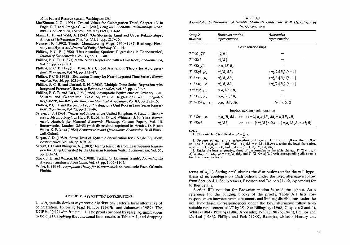
terms of op( 1). Setting e = O obtains the distributions under the null hypo­thesis of no cointegration. Distributions under the fixed alternative follow from Section 4.1. See Kremers, Ericsson and Dolado (1992, Appendix) for further details.

Section I1l's notation for Brownian motion is used throughout. As a reference for the building blocks of the proofs, Table A.1 lists cor­respondences between sample moments and limiting distributions under the null hypothesis. Correspondences under the local altemative follow from suitable replacement of 'B' by 'K'. See Billingsley (1968, Chapters 2 and 4), White (1984), Phillips (1986, Appendix; 1987a; 1987b; 1988), Phillips and Durlauf (1986), Phillips and Park (1988), Banerjee, Dolado, Hendry and

11

346 BULLETIN

Smith (1986, Appendix), and Banerjee, Dolado, Galbraith and Hendry (1992) for derivation of the results in the tableo

The DF Statistic. The DF statistic is:

tOF = (l:w7_1 t 1/2 '(l:W'_ld w,/ae )

= c( T - 2l:w7_l/a;)I/2 + (T- 2l: w7_l/a;t 1/2.( T-1l:W,_1 e,/ a;)+ Op( T-1/2)

(Al)

See Dickey and Fuller (1979) and Phillips (1987a, 1987b) for details. From (Al), the (exact) distribution of tOF is invariant to the scaling of w" and so to the choice of a, aU. and a,. With no cointegration, the last line of (Al) simplifies to (f Be dBe)/J(f B;), the 'Dickey-Fuller' distribution.

The ECM Statistic. The OLS estimator (a by in (3) is:

(A2)

Substituting the definition of dy, into (A2) and pre-multiplying by the matrix diag( T 1/2, T) obtains:

(A3)

The rates of convergence for a and b imply that:

a; = l:i;¡( T - 2).

= a; + Op( T-1 /2). (A4)

By partitioned inversion of the matrices involved in calculating tECM ' and applying the limit results in Table A.1 under the local alternative, the ECM statistic is:

tECM = blese(b)

= c( ael aE ) (T - 2l:w7_11 a;)l/2 + (T - 2l:w7_1 )-1/2( T-1l:w,_1 e,/ aE

)

THE POWER OF COINTEGRATION TESTS

~ c( 1 + q2)1/2(f K;)I/2 + (f Ke dB,)/J(f K;) 347

21/2(f 2)1/2+ (a-1)fK"dB,+s-lfK,dB, ~ c(l + q) Ke J[(a-1)2f K~ + 2(a-1) S -If K"K, +s 2f K;]'

noting (16) and the relation between e" u" and e, (and so between K" Ku, andK.).

U nder the null hypothesis, (A5) simplifies to (15), which itself can be written as (17) when a~ 1 and as the Dickey-Fuller distribution (13) when a = 1. Equations (A3) and (15) correct Banerjee, Dolado, Hendry and Smith ( 1986, Theorem 4).

Under the local alternative, (A5) simplifies to (Al) when a= 1. When a ~ 1, (A5) can be reparameterized in terms of e and q alone, rather than in terms of e, a, and s:

tECM ~ c( 1 + q2)1/2([q2/( 1 + q2)]f K~ - 2[q I( 1 + q2)]f KuK, +( 1 + q2)-1 f K;)l/2

f K" dB,- q-If K, dB, +J[f 2 2 -lfK K + 2fK2) , K,,- q '" q ,

(A6)

noting that (1 + q2) K; = q2 K~ - 2qKuK, + K;. In order to obtain a 'large-q' approximation without having tECM -+ - 00, we hold c( 1 + q2)1/2 constant while expanding in q. Thus, we define a new parameter y, which is:

y=c(1+q2)1/2. (A7)

For large q and constant y, (A6) simplifies to:

tECM~ y(f K~)1/2 +(f Ku dB,)/J(fK~) + Op(q-I). (A8)

Derivation of the distribution of (A8) parallels Phillips and Park (1988, p. 114, Proof of Theorem 2.3). The bivariate Brownian motion (B" KJ' is defined on a probability space, denoted (Q, F, P). Let Fu denote the sub a-field of F generated by Ku. Then the second term on the right-hand side of (A8) is a standardized normal distribution, conditional on Fu (and also unconditionally). Thus, tECM is itself approximately conditionally distributed as a standardized normal variate:

tECM 1"~N(y(fK~)1/2, l)+Op(q-I). (A9)

In essence, (A9) is conditional on {u,}, and so on {z,}. Under the null hypothesis, y = O so tECM is both conditionally and uncondi­

tionally asymptotic N(O,l), to Op(q -1), from Phillips and Park (1988). Comparison of the unconditional distributions of tECM and tOF under the local alternative requires several steps.

12

348 BULLETIN

First, note that the distribution of tOF in (Al) is invariant to q. Thus, for given values of T, e, and its critical value, tOF has a given power, p* (say). Second, (fK;)1/2 in (A9) is non-negative; and, for any O( 1 ~ O> O), there exists a 'IC > O such that:

Prob[(fK~)1/2~ 'IC]> 1- O. (AlO)

Third, note that e is negative; and y in (A9) is e(l + q2)1/2, which is O(q). Now, consider a critical value for tECM equivalent to that for tOFo For sorne q large enough, y(f K~)1/2 [and so tECM itself] is more negative than that critical value with probability arbitrarily close to unity. Thus, for large q, tests using tECM have greater power than those using tOFo

An approximation to the unconditional mean of tECM helps in analyzing the Monte Cario simulations:

(A11)

The two approximations arriving at y[E(f K~)P/2 are standard. The deriva­tion of E(f K~) proceeds as follows.

The integral f K;, can be generated as the large-T limit of T-2"i:.~;/a~ for the process:

(A12)

where p = eclT, e < O, and ~o = O. Without loss of generality, a~ = 1. For any t>O,

E(~n=(l- p2t)/(1- p2) =(1- e2ctIT)/(1- e2clT )

by repeated substitution of (A12). Thus, it follows that:

App.lyingL'Hopital's rule (as T- 00), the large-sample limit of (A14) is:

limT_coE(T-2"i:.~n=(e2c-1- 2e)/(4e2).

(A13)

(A14)

(A15)

Applying L'Hopital's rule again (this time as q - 00 and so as e - O) obtains:

lime_o limT_ co E( T-2"i:.~n = lim,_oe 2c/2 = 1/2. (A16)

13