Human activities and global warming: a cointegration analysis

MPRAMunich Personal RePEc Archive

Human activities and global warming: acointegration analysis

Hui Liu and Gabriel Rodrıguez

University of Ottawa

2005

Online at http://mpra.ub.uni-muenchen.de/9939/MPRA Paper No. 9939, posted 9. August 2008 13:44 UTC

http://mpra.ub.uni-muenchen.de/

http://mpra.ub.uni-muenchen.de/9939/

Human activities and global warming:a cointegration analysis*

Hui Liu, Gabriel Rodrıguez*

Department of Economics, University of Ottawa, P.O. Box 450, Station A, Ottawa, ON, Canada K1N 6N5

Received 25 July 2003; received in revised form 22 February 2004; accepted 30 March 2004

Abstract

Using econometric tools for selecting I(1) and I(2) trends, we found the existence of static long-run steady-state and dynamiclong-run steady-state relations between temperature and radiative forcing of solar irradiance and a set of three greenhouse gases

series. Estimates of the adjustment coefficients indicate that temperature series is error correcting around 5e65% of the disequilibriaeach year, depending on the type of long-run relation. The estimates of the I(1) and I(2) trends indicate that they are driven by linearcombinations of the three greenhouse gases and their loadings indicate strong impact on the temperature series. The equilibrium

temperature change for a doubling of carbon dioxide is between 2.15 and 3.4 (C, which is in agreement with past literature and thereport of the IPCC in 2001 using 15 different general circulation models.� 2004 Elsevier Ltd. All rights reserved.

JEL classification: C22; Q00

Keywords: Global warming; Radiative forcing; Cointegration; I(1) process; I(2) process; Unit roots

1. Introduction

One of the main conclusions achieved by theIntergovernmental Panel on Climate Change (IPCC,2001) is that temperature series is warming for the past150 years. Furthermore, the same reference attributesthe responsibility of the changes to human activitiesgenerated greenhouse gases. A basic argument in thisdiagnostic is that temperature series are higher com-pared to the pre-industrial periods; see also Santer et al.(1996). There are two sources for this evidence. Theyare the physically-based simulation models of climateand the statistical analysis of historical data, respec-tively. The simulation models of climate are based onphysical motion equations trying to describe the princi-pal issues governing the behavior of temperature. Theyalso include the radiative forcing of greenhouse gases

and tropospheric sulfates. This kind of model are gen-erally referred as general circulation models (GCMs).

On the other hand, the statistical analysis dealsdirectly with the historical record of the temperaturevariables, solar irradiance and greenhouse gases. Insome cases, this approach uses simple and standardstatistical or econometric tools in identifying for theeffects of human activities (greenhouse gases) on thetemperature series. However, because all these timeseries exhibit strong trends, classical tools will indicatespurious positive relation among these variables. Inconsequence, it is important to identify clearly the timeseries properties of the data before starting any otherkind of analysis between the series. In this aspect, theprincipal goal is the identification for the existence ofunit roots in the data which means the existence ofstochastic trends. It is the starting point of the researchagenda of Stern and Kaufmann (1997, 1999, 2000) andKaufmann and Stern (2002).1 Using different statistical

www.elsevier.com/locate/envsoft

Environmental Modelling & Software 20 (2005) 761e773

* This paper is drawn from the first chapter of the Ph.D.

dissertation of Hui Lui at the University of Ottawa.

* Corresponding author. Tel.: C1-613-562-5800; fax: C1-613-562-

5999.

E-mail address: [email protected] (G. Rodrıguez).

1 See next section for a brief but more complete survey of the

literature.

1364-8152/$ - see front matter � 2004 Elsevier Ltd. All rights reserved.

doi:10.1016/j.envsoft.2004.03.017

http://www.elsevier.com/locate/envsoft

mailto:[email protected]

tests for the identification of unit roots, they find thattemperature series is an I(1) process,2 and that green-house gases contain two unit roots. After analyzing forcausality between different set of time series, Stern andKaufmann (1997) investigate the existence of long-runsteady-state relations (i.e. cointegration between sets ofvariables) using multivariate techniques proposed byJohansen (1988, 1995b). They conclude that there existsa long-run relation between the set of variables and thattemperature series is reacting to the disequilibriatowards this steady-state relation in around 40e50%each year. However, the authors believe that this value istoo high and it may be a consequence of the existence ofI(2) trends in the system. Kaufmann and Stern (2002)recognizes the necessity to take into account for I(2)trends in an adequate statistical framework.

The statistical framework for I(2) is proportionatedby the approach suggested by Johansen (1992, 1995a);see also Paruolo (1996); Rahbek et al. (1999); Paruoloand Rahbek (1999). It is more complex but richer interms of the long-run relations that we may find. In fact,there are the standard (static) long-run steady-staterelations but there also exist the dynamic long-runsteady-state relations which are given by the linearcombinations between the levels of the variables andtheir first differences. It is also possible to find medium-run steady-state relations. In this paper, we follow thisapproach.

The empirical results show that global temperatureand solar irradiance series are I(1) processes, carbondioxide is an I(2) process, and methane and nitrousdioxide seem to contain explosive roots. According tothis evidence, three different systems are proposed,estimated and analyzed. The results indicate thattemperature series is error correcting around 10e50%of the disequilibria each year, depending of the type ofsteady-state relation that is considered. Regarding theequilibrium temperature change for a doubling ofcarbon dioxide, the results indicate that it is between2.1 and 3.4 (C, depending of the steady-state used tocalculate it. It is worth noting that these values are inagreement with other values found in the literature (seeKaufmann and Stern, 2002) and the average valuecalculated by the Intergovernmental Panel on ClimateChange (IPCC, 2001).

The rest of this paper is organized as follows. Section2 presents a brief review of the literature. Section 3 dealswith the methodological issues while Section 4 presentsthe empirical results. Section 5 concludes.

2. A brief review of the literature

In order to place this work in the context of theliterature on climate change, a brief summary of some ofthe relevant papers is provided below. When we observepictures of global temperature series, greenhouse gasconcentrations, and solar irradiance, all give us theinformation that they have increased in the last 150years; see also Stern and Kaufmann (2000). Presence ofstrong trends implies that the use of standard statisticalor econometric tools will indicate a significant andpositive association between sets of variables analyzed.Unfortunately, the use of standard statistical or eco-nometric tools is misleading in this context. Therefore,a careful analysis of the statistical properties of the timeseries appears as a necessary condition for an adequateempirical analysis. This is the starting point of theresearch applied by Stern and Kaufmann (1997, 1999,2000), and Kaufmann and Stern (1997, 2002). Apartfrom them, there is little research that explicitly arguedin favor of the use of econometric time series methods,such as Tol (1994), Tol and de Vos (1998), andSchonwiese (1994). Some other exceptions in the anal-ysis of the time series properties of global temperatureseries are Bloomfield (1992), Bloomfield and Nychka(1992), Woodward and Gray (1993, 1995), Galbraithand Green (1993); Richards (1993); Fomby andVogelsang (2002). Before them, most of the researchanalyzing the relationship between temperature andforcing variables have used simple regression models asin Lean et al. (1995), or frequency domain methods as inKuo et al. (1990) and Thomson (1995, 1997).

The analysis of the time series properties of tempera-ture, solar irradiance, greenhouse gases and othervariables has been performed in Stern and Kaufmann(1997). One of the principal conclusions of their researchis that global temperature series has a unit root or in otherterms, this time series has a stochastic trend, which isdenoted by I(1). At the same time, greenhouse gasesvariables have been found to contain one or two unitroots. The econometric tools used were the well knownunit root statistics proposed by Dickey and Fuller (1979),Said and Dickey (1984), Phillips and Perron (1988), andSchmidt and Phillips (1992). As a consequence of the sizeand power problems of these unit root statistics indetecting for more than one unit root,3 there is not acomplete and clear picture regarding the degree ofintegration of the greenhouse gases. However, the evi-dence in favor of twounit roots is present inmore thanoneunit root test. It is also recognized in Stern andKaufmann(1999, 2000), and Kaufmann and Stern (2002).

When the time series are non-stationary there is roomto test for cointegration, that is, the possible existence of2 A time series yt is integrated of order d, which is denoted by I(d ) if

d differences are needed to transform it into a stationary time series.

Therefore, I(1)/I(2) means that the series has to be differenced one/two

times to achieve stationarity. 3 See Haldrup and Lildholdt (2002).

762 H. Liu, G. Rodrıguez / Environmental Modelling & Software 20 (2005) 761e773

long-run relationships between sets of variables ana-lyzed. In other words, it is possible to find linearcombinations of the variables that annihilates thestochastic trends. The rest of linear combinations arestill stochastic trends and they drive the behavior of thetime series. The cointegrating relations are named alsostatic long-run relations because they represent a steady-state relation between sets of variables. Because in theshort term the variables are not in the steady state, theywill react to these disequilibria. In the case of tem-perature, for example, it is possible to find a steady-staterelation with greenhouse gases and natural factors (solarirradiance, for example). In the short term, the tem-perature (and the other variables) reacts to the dis-equilibria exhibiting an error correction behavior.

The only two trials to deal with the identification ofcointegration relations have been Stern and Kaufmann(1997) and Kaufmann and Stern (2002). Using themethodology of Johansen (1988, 1995b),4 they arrive atthe conclusion that there exists a long-run relationshipbetween time series of temperature, solar irradianceand a set of greenhouse gases. The estimates of theshort-run dynamic model indicate that temperature iscorrecting around 40e60% of the disequilibria eachyear. The authors consider that this value is too highand they attribute its cause to the existence of I(2)trends.

The acceptation that time series of greenhouse gasescontain I(2) trends is also present in Stern andKaufmann (1999, 2000). In both papers, the authorsapply a multivariate structural time series approach tomodel temperature, natural factors and greenhousegases.5 The advantage of this kind of models is thatdifferent alternatives for the deterministic componentsare allowed. Also, it is possible to allow for I(1) and I(2)trends. The model is also flexible in including cyclicalcomponents. The basic conclusions are that most timeseries analyzed contain a stochastic trend with thegreenhouse gases containing stochastic I(2) trends.Therefore, the two independent stochastic trends in thedata are associated to the radiative forcings due togreenhouse gases, solar irradiance, and troposphericsulfate aerosols that are found in the northern hemi-sphere, respectively. More recent research but applied tothe temperature of Australia is Lenten and Moosa(2003). According to their results, temperatures in sixAustralian locations are I(1) processes, the cyclicalcomponent is not significant, seasonality is deterministicand the irregular (or noise) component is very significant.

On the other hand, some different results areproportionated by Kelly (2000). He finds that temper-ature series contains a unit root but that greenhouse

gases are stationary around a time trend. This impres-sive result implies that temperature rise is due to longrun cycles, and that the relationship with greenhousegases is spurious. These results are in completeopposition to most of the research detailed before.However, applying first difference to temperature series,Kelly (2000) estimated a regression between growthrates of temperature and greenhouse gases, findingsupport to previous results regarding the significantinfluence of these gases on temperature series.

One important and uncertain parameter of thegeneral circulation models (GCMs) is the temperaturesensitivity which is measured as the equilibriumtemperature change per unit of the change in radiativeforcing. As Kelly (2000) argues, an alternative measure,directly proportional to the climate sensitivity, is thetotal equilibrium (steady-state) temperature changefrom a doubling of greenhouse gases, frequentlydenoted as DT2x. Kelly (2000) finds that this parameteris between 1.27 and 1.33 (C; while for Kaufmann andStern (2002) its value is around 2.0 and 2.5 (C, inagreement with the general circulation models. It isworthwhile to mention that the IPCC (2001) argues thatthe average value of DT2x is 3.5 (C after considering15 different models.6

In this paper we still use time series tools to analyzefor the existence of steady-state relations between temp-erature series, solar irradiance and a set of greenhousegases. However, unlike the traditional approach of usingthe so called I(1) model, as Stern and Kaufmann (1997)and Kaufmann and Stern (2002), we use econometrictools allowing for the presence of I(2) trends in theidentification of the long-run relationships. The use ofmore sophisticated econometric tools taking into ac-count for the presence of I(2) trends has been recognizedby Stern and Kaufmann (1999). The presence of twounit roots in time series allows us to use the so called I(2)model (see Johansen, 1992, 1995a, 1995b). In this modelthe number of cointegrating relations are detected, soare the number of I(1) and I(2) stochastic trends that stillin the system and drive the behavior of some variables.In terms of the cointegrating relations, unlike theanalysis of the I(1) model, the I(2) model allows forthe existence of two types of cointegration. The first typeis a linear combination of the variables in their levels,which is the same definition as that in the I(1) model.The second type of cointegration is the possibility thatthere are linear combinations between the levels of thevariables and their growth rates. It is named polynomialcointegration and also dynamic steady-state relations.Further details of I(1) and I(2) models are presented inthe next section.

4 See the I(1) model below for further methodological details.5 This methodology is based on Harvey (1989).

6 The standard deviation is 0.92 (C and the range goes from 2.0 to

5.1 (C.

763H. Liu, G. Rodrıguez / Environmental Modelling & Software 20 (2005) 761e773

3. Methodological issues

In this section we provide elements relevant to under-standing the methodological approach applied in theempirical analysis. Regression with nonstationary timeseries implies spurious regression except when thereexists a linear combination (or more than one) betweenthese variables that reduce the dimension of the spacespanned by them. This is known as cointegration.

3.1. The I(1) model

Let yt, a vector containing n variables, be representedby the following VAR(k):

yt ¼Xk

i¼1

Pyt�iCFDtC3t ð1Þ

where it is assumed that 3t is a sequence of i.i.d. zeromean with covariance matrix U. In most cases it is alsoassumed that the errors are Gaussian which is denotedby 3twN (0,U). The variable Dt contains the possibledeterministic components of the process, such as a con-stant, a time trend, seasonal dummies and interventiondummies. This is the model proposed by Johansen(1988, 1995b) and is widely used in empirical applica-tions.7

The system (1) is reparameterized as a vector errorcorrection model (VECM):

Dyt ¼ Pyt�1CXk�1

i¼1

GiDyt�iCFDtC3t ð2Þ

with

P ¼ �ICXk

i¼1

Pi; Gi ¼Xk

j¼iC1

Pj:

Notice that the matrix

G ¼ I�Xk�1

i¼1

Gi:

I(1) cointegration occurs when the matrix P is ofreduced rank, r!n where P may be factorized intoP=ab#, a and b are both full rank matrices ofdimension n!r; the matrix a contains the adjustmentcoefficients and b the cointegration vectors. Thesevectors have the property that b#yt is stationary, eventhough yt itself is non-stationary. Notice that there alsoexist full rank matrices at and bt of dimensionn!(n�r) which are orthogonal to a and b, such thata#ta=0 and b#tb=0, and the rank(bt,b)=n.

An alternative representation of the cointegratedVAR model is in terms of the common stochastic trendsrepresentation, see Stock and Watson (1998). Accordingto that, the yt vector is represented by

yt ¼ FDtCCXt

i¼1

3iCCðLÞ3t ð3Þ

where C=bt(a#tGbt)�1a#t and C(L)3t corresponds toa n-dimensional I(0) component. Using this representa-tion it is possible to observe that although yt isn-dimensional, the vector series is driven by just n�rcommon stochastic I(1) trends which are

a#tXt

i¼1

3i:

In terms of observable variables the I(1) directions arecalculated as b#tyt which are just a particular linearcombinations of the stochastic trends.

To test the rank of matrix P, Johansen (1995a,b)developed maximum likelihood cointegration testingmethod using the reduced rank regression techniquebased on canonical correlations. The procedure consistsof obtaining an n!1 vector of residuals r0t and r1t fromauxiliary regressions (regressions of Dyt and yt�1 ona constant and the lagged Dyt�1.Dyt�kC1). Theseresiduals are used to obtain the (n!n) residual productmatrices:

Sij ¼ ð1=TÞXT

t¼1

ritr#it; ð4Þ

for i, j=0, 1. The next step is to solve the followingeigenvalue problem

KlS11 � S10S�100 S01 K ¼ 0 ð5Þ

which gives the eigenvalues l1R.Rln and the corre-sponding eigenvectors b1 through bn, which are also thecointegrating vectors. A test for the rank of matrix P

can now be performed by testing how many eigenvaluesl equals to unity. One test statistic for the resultingnumber of cointegration relations is the Trace statistic(see Johansen, 1988), which is a likelihood ratio testdefined by

Trace ¼ �TXn

i¼rC1

logð1� liÞ ð6Þ

Another useful test is given by testing the significanceof the estimated eigenvalues themselves

lmax ¼ �T logð1� liÞ: ð7Þ

In trace test, the null hypothesis is r=0 (no cointegration)against the alternative hypothesis that r O 0 (cointegra-tion). The lmax statistic tests the null hypothesis that r=r0versus the alternative hypothesis that r=r0C1, where

7 There are large number of empirical applications using this

statistical framework. Two very detailed and influential applications

are Johansen and Juselius (1992 and 1994).


r0=0, 1,., n�1. For further details regarding theconstruction of these statistics, see Johansen (1995b).

In summary, the I(1) model allows to identify therank of cointegration (r) and the number of stochastictrends driving the yt vector. Because in this model it isassumed that yt contains variables with order of integra-tion no larger than one, it is clear that the number ofunit roots left in the system is n�r. Notice that theestimate of b (the cointegration vector) is not identifiedin the sense that any linear combination of b is alsoa cointegration vector. In this sense, researchers have toidentify these vectors by imposing restrictions that are inmost cases suggested by the economic theory. Forexample, in a vector containing four variables, a possiblerestriction is that the coefficient associated to the secondvariable is zero. If the statistic (distributed as a c2) doesnot reject the null hypothesis, it means that the secondvariable is long-run excluded from the cointegrationvector. Another example is the restriction of long-runhomogeneity between a set of variables. If the nullhypothesis is not rejected, it means that the unit vector(i.e. [1, �1,., �1]) may be used in the subsequentanalysis. The estimated adjustment coefficients (a) arealso tested for restrictions but in this case, therestrictions are associated with the null hypothesis ofweak exogeneity.

3.2. The I(2) model

In the I(1) model, the matrixP is of reduced rank andthe matrix a#tGbt is of full rank. For the system to beI(2) it is also required that the matrix a#tGbt be ofreduced rank s1!n�r. Following Johansen (1992,1995a,b), the model (2) can be reparameterized as

D2yt ¼ Pyt�1 � GDyt�1CXk�2

i¼1

JiD2yt�iCFDtC3t ð8Þ

where the matrix G is included as a parameter and

Ji ¼ �Xk�1

j¼iC1

Gj:

With the matrix a#tGbt of reduced rank (sq), it ispossible, as in the I(1) model, to define parametermatrices x and h such that the second reduced rankcondition is a#tGbt=zh# with z and h both matrices ofdimension (n�r)!s1.

As in the I(1) model, the number of cointegrationrelations (or I(0) relations) is denoted by r. However,unlike I(1) models, n�r does not only represent thenumber of I(1) trends in I(2) models. It contains boththe total of I(1) trends and that of I(2) trends, denoted ass1 and s2, respectively. Consequently there are param-eters describing the I(0), I(1) and I(2) directions of the

variables and an important goal of the I(2) model is theiridentification. Following the notation of Juselius (1999),these matrices are b, bt1 and bt2 associated withdimensions r, s1 and n�r�s1=s2 respectively.8 Paruolo(1996) denotes r, s1, s2 as the integration indices ofthe VAR.

In a similar way as in the I(1) model, the commontrends representation of I(2) model is given by

yt ¼ FDtCC2

Xt

j¼1

Xj

i¼1

3iCC1

Xt

i¼1

3iCC �ðLÞ3t ð9Þ

where C2 ¼ bt2ða#t2Qbt2Þ�1a#t2 and C*(L) is a matrix

polynomial with all roots strictly outside of the unitcircle. The first clear observation is that yt has s2common I(2) trends given by

a#t2

Xt

j¼1

Xj

i¼1

3i:

In terms of observable variables, it is given by b#t2ytwhich are just linear combinations of the I(2) stochastictrends.

Furthermore, as mentioned by Haldrup (1999), thecombinations b#yt can cointegrate to I(0) level and/orhave the property that they potentially cointegrate withb#t2Dyt, which is I(1) by construction. This is named aspolynomial cointegration. These r relations are b#yt�db#t2Dyt which define the I(0) directions. However, notall the r I(0) relations need include the differenced I(2)components. In fact, after defining dt such that d#td=0,there will be r�s2 non-polynomially cointegratedrelations given by d#tb#yt; and s2 polynomial cointegrat-ing relations given by d#b#yt�d#db#t2Dyt.

9

The approach suggested by Johansen (1992, 1995b)to identify the number of I(2) trends is conducted asa combination of regression and reduced rank re-gression. It is performed in a similar way as the deter-mination of the cointegration rank in the I(1) model.The difference is that now two reduced rank conditionsneed to be examined. This is more complicated in thesense that the second reduced rank condition dependson the first reduced rank condition. Instead of a joint

8 The notation and technical details of the I(2) model are complex.

Further details regarding the calculation of matrices bt1 and bt2 are

in Juselius (1999), also Haldrup (1999) using a slightly different

notation. In summary, because z and h exist, their complements, ztand ht, also exist. Then it is possible to define atZ{at1, at2} and

btZ{bt1, bt2}, where at1Zat(a#tat)�1z at2Zatzt, bt1Zbt(b#tbt)�1h and bt2Zbtht. Therefore, b, bt1 and bt2 are

mutually orthogonal and thus jointly describe a basis for the

n-dimensional space. The a has a similar property.9 The possibility to decompose r (in r0 and r1, say) exists only when r

O s2. In this case, the r cointegrating relations can be divided into

r0Zr�s2 directly stationary CI(2,2) relations and r1Zs2 polynomially

cointegrating relations.


estimation of the indices r and s1, Johansen (1992, 1995a)suggests a two step procedure. The first step is to solve thereduced rank problem associated with the matrixP=ab#. It calculates the estimates of ar, br, atr, andbtr for each value of r=0, 1,., n�1. The second stepdeals with the second reduced rank condition problem byreplacing the unknown matrices atr, and btr with theestimates from the first step. The problem is solved for ors1=0,.,n�r�1. Then what remains to be determined iswhich combinations of r and s1 should be chosen. Becausesteps 1 and 2 proportionate an array of different valuesfor r and s1 corresponding to different sub-models, theselection of r and s1 can be performed in the followingway.10 The array is read starting from the left corner. Ifthe null hypothesis is rejected, the next element (continu-ing to the right) is read and so on. After the first row isdone, and if no acceptation is observed, we read thesecond row of the array. We continue until the first non-rejection is found. The associated values of r, s1 and s2 areselected as the integration indices. Complete technicaldetails can be found in Paruolo (1996); Johansen (1992,1995a).

It must be emphasized that only the space spanned bythe cointegrating vectors is identified; the single cointe-gration relations are unidentified. This issue is alsopresent in the I(1) model but this problem is morecomplex in I(2) models.11

What is perhaps more interesting is the fact that in anI(2) model there exist more than one steady-state rela-tions. Recall that in an I(1) models, the cointegrationrelations b#yt represents the static long-run steady-staterelation. In the present case, we have two additionalsteady-state relations. One is medium-run steady-staterelations represented by b#t1Dyt. The other is dynamiclong-run steady-state relations represented by the poly-nomially cointegrating relations (see Juselius, 1999, 2003).In consequence, there exist different adjustment coeffi-cients associated with each of these steady-state relations.

One should keep in mind that tools for analyzing I(2)models and statistics used to select integration indexesare not yet fully developed in econometric literature.This is the reason why the selection of the number of I(2)trends should be combined with other tools. One ofthem, as suggested by Juselius (1999), is the calculus ofthe roots of the companion matrix. If yt vector containsvariables that are integrated no more than order one,then the total number of unit roots (or close to the unitcircle) of the companion matrix must be n�r. If thereexists more than n�r roots close to the unit circle, it

constitutes a indicator for the presence of I(2) trends.When there are I(2) trends, the number of roots close tothe unit circle is s1C2s2.

Another useful indicator for the presence of I(2)trends is to compare the graphs of b#yt and b#R1t, whereR1t is a vector of residuals from regressing yt�1 onlagged short-run effects (Dyt�i, i=1, 2,., k�1) and Dt.If the first graph looks non-stationary whereas thesecond graph looks stationary, it can be considered asa strong support for the presence of I(2) trends.

Recently a few empirical applications in the field ofeconomics have used the I(2) framework. Without theintention to be exhaustive, some of these references areRahbek et al. (1999), Kongsted (2003), Holtemoller(2002), Vostroknutova (2003), Juselius (1999, 2003),Fiess and MacDonald (2001), and Haldrup (1999). It isworthwhile to mention that some of these papers, afteridentifying for the presence of I(2) trends, proceedwith transforming the variables in such a form thata standard I(1) analysis can be performed (see Fiess andMacDonald, 2001). Almost all references mentionedstudy nominal variables such as money supply, nominalwages, and fundamentally prices. We do not know thata similar methodology has been applied to climate series.

4. Empirical analysis

4.1. The data and preliminary issues

The data used in this paper include the time series ofglobal mean temperature deviation (denoted by temp),the concentrations of methane (ch4), nitrous dioxide(n2o), carbon dioxide (co2).

12 All data are from the website of Goddard Institute for Space Studies available athttp://www.giss.nasa.gov. The data are transformedinto radiative forcing,13 which affects the temperature

10 The test statistic is denoted as Hr,s and it is the same notation

used in the empirical analysis.11 Regarding the adjustment coefficients, for example, the notion of

weak exogeneity is now different. Paruolo and Rahbek (1999) have

proposed a sequential approach to test for weak exogeneity in the I(2)

model.

12 A preliminary version of the paper included data of chlorofluor-

ocarbons (cfc11 and cfc12). Graphical inspection of both time series

indicates zero values until 1950, after what they increased very fast.

These two variables were found to be I(2) processes in Stern and

Kaufmann (2000).We decided exclude both time series for the following

reasons: (i) the visual analysis indicates a particular behavior that may

distort the analysis; (ii) their importance in terms of all greenhouse is

reduced; (iii) increasing the dimension of the system of equations to be

estimated, therefore reducing the number of freedom degrees given our

sample size; and (iv) identification of cointegration relations is complex

and unlike the field of economics, we are not sure what are the physical

relationships and interactions between all these greenhouse gases series,

solar irradiance and temperature time series. Therefore, by excluding

both variables, we reduce the possibility to find too many cointegration

relations which are always difficult to identify and interpret.13 Radiative forcing is the change of the net irradiance caused by

factors such as greenhouse gases, water vapor, solar radiation.

Greenhouse gases are of particular interest, as they are most likely

to change radiative forcings over the next decade. The net irradiance is

the difference of the irradiance that the earth absorbed minus the

irradiance the earth emitted, expressed inWm�2, whereW is a measure

of energy (Watt) and m indicates meters.


http://www.giss.nasa.gov

directly and indirectly. The formulae are tabulated in theIntergovernmental Panel of Climate Change (IPCC,2001). Therefore the radiative forcing of greenhousegases at time t are denoted by r f ch4t, r f n2ot, r f co2t. Wealso include radiative forcing of solar irradiance (r f sunt)as another variable in the system.

Fig. 1 presents the evolution of the time series for theperiod under study, 1856e2001. It is a similar period asanalyzed by the previous literature but with more recentinformation. A clear observation appearing from Fig. 1is the fact that all greenhouse gases variables presentstrong upward trends that have been observed in theprevious literature.

As that argued in the literature (Stern and Kaufmann,2000), an essential preliminary step in the analysis ofthese variables is the identification of the time seriesproperties. One way to approach this issue is theapplication of univariate unit root tests. Stern andKaufmann (2000) proceeded using three different uni-variate unit root tests. However, as documented byHaldrup and Lildholdt (2002), these statistics areincorrect. Because when testing for I(2) and the un-derlying series is indeed integrated of order two, thesestatistics give rise to an excessive rejection of the nullhypothesis of a unit root in favor of the stationary andexplosive alternatives. This size distortion is causedby the fact that the test statistics have a different dis-tribution originated by one additional unit root. Inconsequence, the recommendation of Haldrup and

Lildholdt (2002) is to test I(2) against I(1) priorto testing I(1) against I(0). The authors conclude thatall basic univariate unit root tests suffer from thisissue.

In a set of results not reported here,14 we applied theapproach suggested by Dickey and Pantula (1987) andalso the statistic proposed by Hasza and Fuller (1979).The results indicated that the carbon dioxide seriescontains two unit roots, that is, it is an I(2) process. Thetemperature and solar irradiance series were found to beI(1) processes, the other greenhouse gases series understudy (nitrous dioxide and methane) appeared contain-ing explosive roots. The last result is not totally clearafter the application of all statistics. The difficulty withthis case is the fact that explosive roots mimic thebehavior of I(2) processes, see Haldrup and Lildholdt(2002).

In summary, most of the results confirm the previousresults found in the literature, see Stern and Kaufmann(2000). Although it appears to be the case, we adoptanother strategy in this paper. This approach consists ofapplying multivariate techniques to detect the number ofI(0), I(1) and I(2) trends in the system. As we will see in

1850 1900 1950 2000

-0.5

0.0

0.5 temp

1850 1900 1950 2000

-0.2

-0.1

0.0

0.1 rfsun

1850 1900 1950 2000

0.5

1.0

1.5rfco2

1850 1900 1950 2000

0.2

0.4rfch4

1850 1900 1950 2000

0.05

0.10

0.15rfn2o

Fig. 1. Global temperature deviations (temp), radiative forcing of solar irradiance (rfsun), carbon dioxide (rfco2), methane (rfch4) and nitrous dioxide

(rfn2o); units in Wm�2; 1856e2001.

14 But they are available upon request. We applied standard ADF

test (Dickey and Fuller, 1979; Said and Dickey, 1984), Phillips-Perron

test (Phillips and Perron, 1988), and ADF based on GLS detrended

data as suggested by Elliott et al. (1996).


the next analysis, there are more than one possible casein the selection of the integration indices.15

4.2. The first case

The first case is represented by the system with ourfive variables, i.e., yt={tempt, r f sunt, r f co2t, r f ch4t, r fn2ot}. Table 1 presents the results obtained from theapplication of the approach of Johansen (1988, 1995b)in determining the rank of matrix P16. Both Trace andlmax statistics indicate that r=3, that is, there exist threecointegration relations. Because n=5, we haves1Cs2=n�r=2.

Table 2 presents the results of the statistic Hr,s forselecting s2. The first row represents the value of thestatistic, the second and third rows are the critical valuesat 95.0% and 97.5% (in italics). As we explained in theprevious section, reading of this table starts from theleft-corner and we continue to the right. If noacceptation is found, we continue to the second row ofvalues (r=1). The procedure stops when a non-rejectionis found. In the present case, the results indicate thats2=0 and consequently s1=2. Then, there are two I(1)trends and there is no I(2) trends in the system.However, note that using critical values at 97.5%, it ispossible to find s2=1 and consequently s1=1.

As suggested by Juselius (1999), a good way tocomplement this information is the calculus of theeigenvalues of the companion matrix. The eight largestmodules obtained from the unrestricted VAR are:1.0292, 1.0292, 0.9641, 0.9641, 0.9384, 0.9384, 0.7163,0.7163. It appears to exist two explosive roots and foureigenvalues close to the unit circle. In other words, thereappears to exist four unit roots in the system. Now,

because the first step (in the I(1) framework, see Table 1)indicates r=3, we proceed with imposing this restrictionand now the eight largest modules of the restricted VARare: 1.0283, 1.0283, 1.000, 1.000, 0.9378, 0.9378, 0.7179,0.7179. There are two unit roots as a consequence of therestriction of r=3 but there are two more eigenvaluesclose to the unit circle. It indicates, again, the existenceof four unit roots.17 Remember that in the I(2)framework the total number of unit roots is given bys1C2s2, which in the present case indicates that s1=0and s2=2.

In summary, we have some different informationusing the Hr,s statistic and the eigenvalues of the com-panion matrix. We decide to working with both alter-natives. Then, they are r=3, s1=1, s2=1 and r=3,s1=0, s2=2, respectively. In the following, they arenamed as Case 1 and Case 2, respectively.

Following the notation used in the previous section,Table 3a presents cointegration relations and adjust-ment parameters corresponding to Case 1. Notice thatthere are two cointegrating relations including only thelevels of the variables ðb0;iyt; i ¼ 1; 2Þ: Furthermore, therelation b1yt � k1Dyt denotes the polynomially cointe-gration relation or what we denoted in the previoussection as the dynamic steady-state relation. The bottompanel gives the corresponding loadings ða0;1; a0;2; a1Þ:and the coefficients that reflect the composition of thestochastic I(1) and I(2) trends at1 and at2: The tablealso presents vectors bt1 and bt2 that denote theloadings (adjustment parameters) to the stochastic I(1)and I(2) trends.

Table 3a specifies that around 46.6% of the dis-equilibrium in the static long-run steady-state is

Table 1

Testing for cointegrating ranks

H0 lmax Trace lmax 90%

critical values

Trace 90%

critical values

r=0 83.6 196.2 34.8 82.7

r=1 49.4 112.5 29.1 59.0

r=2 41.9 63.1 23.1 39.1

r=3 14.2 21.3 16.9 23.1

r=4 7.1 7.1 10.5 10.6

Yt ¼ ðtempt; r f sunt; rfco2t; rfch4t; rfn2otÞ#.

Table 2

Testing for integration indices

r Hr,s Qr

0 418.0 312.6 252.0 220.8 198.2 196.2

(198.2) (167.9) (142.2) (119.8) (101.5) (87.2)

(203.2) (173.4) (147.1) (124.4) (105.6) (91.2)

1 268.6 171.4 136.8 114.8 112.5

(137.0) (113.0) (92.2) (75.3) (62.8)

(141.5) (117.4) (96.5) (79.0) (66.1)

2 163.4 91.2 69.0 63.1

(86.7) (68.2) (53.2) (42.7)

(90.8) (71.4) (55.9) (45.8)

3 57.9 36.2 21.3

(47.6) (34.4) (25.4)

(50.7) (36.8) (27.9)

4 15.3 7.1

(19.9) (12.5)

(22.2) (14.2)

n�r�s=s2 5 4 3 2 1 0

Yt ¼ ðtempt; rfsunt; rfco2t; rfch4t; rfn2otÞ#:

15 Analysis of I(1) and I(2) models was performed using CATS for

RATS, see Hansen and Juselius (1995). A slightly modified version of

the program of Rahbek et al. (1999) has been used. We also thank

electronic communications with H.C. Kongsted who proportionated

his program used in Kongsted (2003). The estimations of the error

correction models were performed using PcGive 10.0, see Doornik and

Hendry (2001).16 In all cases, we consider linear trends in the data. An intercept

and a time trend are also allowed in the cointegration space. In terms

of the I(2) framework, it is the model suggested by Rahbek et al.

(1999).

17 Notice that the two explosive roots seem to confirm the

univariate analysis.


corrected by the temperature series each year. This issimilar as that found by Stern and Kaufmann (2000).On the other hand, the result that temperature series donot react to the second static long-run relation is alsointeresting. The response of the temperature series to thedynamic steady-state relations is 19.1%. As we know,these dynamic steady-state relations ( polynomiallycointegration relations) include the levels and thegrowth rates of the variables. Therefore, the resultindicates the response of temperature series to disequi-libria towards the steady-state. Regarding to themedium-run steady-state relation ðbt1DytÞ, we observethat it is composed by temperature, solar irradiance,carbon dioxide and methane series.

Regarding the stochastic I(1) and I(2) trends, we havethe following observations. Firstly, it appears that bothI(1) and I(2) trends are driven by three greenhouse gasesðat1; at2Þ, whereas the influence of methane andnitrous dioxide is higher in stochastic I(2) trend ðat2Þ:In other words, permanent shocks to the threegreenhouse gases seem to have generated the I(2) trend.Secondly, the respective loadings (or adjustment param-eters) to these stochastic I(1) and I(2) trends indicatethat temperature series, solar irradiance and carbondioxide are influenced by them ðbt1; bt2Þ: The resultsalso show that temperature, carbon dioxide, and solarirradiance are more influenced by the stochastic I(1)trend ðbt1Þ: However, the stochastic I(2) trend seems toaffect strongly the temperature series ðbt2Þ:

Regarding the equilibrium temperature change fora doubling of carbon dioxide (DT2x), the results indicatethat it is 3.4 (C; see the first long-run steady-staterelation. This value is higher than those found in theliterature but it is in agreement with the average ofestimates from 15 general circulation models coupled tomixed-layer ocean models reported in IPCC (2001).

Table 3b proportionates similar information but forthe case r=3; s1=0; s2=2. In this case the results showthat there is only one static long-run steady-state

relation and two dynamic steady-state relations. Theloading corresponding to the long-run steady-state rela-tion seem to indicate that temperature series is not errorcorrecting which may indicate that the disequilibria arenot corrected at all. The response to the dynamic steady-state is, as before, higher and with the correct sign. Infact, it appears that temperature series is correcting4.8% and 64.6% (each year) of the disequilibria pre-sented in these relations.

Because in this case s1=0, there are not I(1) trends inthe system. The two I(2) trends seem to be driven bycarbon dioxide and nitrous dioxide in the first caseðat2;1Þ and by the three greenhouse gases in the secondcase ðat2;2Þ. Observing the coefficients in bt2;1 andbt2;2, it is clear that the higher influence (in both cases)is on temperature series. All these results confirm theanalysis of Kaufmann and Stern (2002).

4.3. The second case

Univariate and multivariate analysis seem to indicatethat there are explosive roots in the system. Therefore,an alternative analysis is to separate the five-variablesystem into two sub-systems. The first system containsthree variables: temperature, solar irradiance and car-bon dioxide. The second system has two variables:methane and nitrous dioxide, the two variables thatseem to have explosive roots.

Tables 4a and b present the Trace and lmax statistics.Notice that the selection of the rank of matrix P is valideven when there are explosive or I(2) trends, see Nielsen(2001, 2002). Table 4a (3-variables system) indicates thatr=1. The same result is found for Table 4b (2-variablessystem).

Tables 5a and b present the results from the Hr,s

statistic. The numbers in italic are critical values at95% quantiles. In the case of the 3-variables system(Table 5a), we found s2=1 and consequently s1=1.The seven largest modules of the companion matrix

Table 3a

Decomposing the systems into I(0), I(1) and I(2) spaces; Case 1

b0;1 b0;2 b1 k1 bt1 bt2

temp 1.000 1.000 1.000 �79.039 �3.921 �5.698

rfsun �0.078 �4.639 �1.638 �26.868 �3.006 �1.937

rfco2 �0.792 �2.161 7.303 �35.985 9.647 �2.594

rfch4 0.928 5.565 �22.491 �21.236 2.074 �1.531

rfn2o �36.398 2.774 96.030 �1.872 �0.258 �0.135

trend 0.015 0.004 �0.050

a0;1 a0;2 a1 at1 at2

temp �0.466 0.067 �0.191 �0.000 �0.001

rfsun �0.034 0.096 �0.014 �0.001 �0.002

rfco2 �0.015 0.010 �0.005 0.007 �0.007

rfch4 �0.003 0.002 �0.002 0.011 0.095

rfn2o �0.000 0.002 0.000 �0.009 0.125

Yt ¼ ðtempt; rfsunt; rfco2t; rfch4t; rfn2otÞ#.

Table 3b

Decomposing the systems into I(0), I(1) and I(2) spaces; Case 2

b0 b1;1 k1 b1;2 k2 bt2;1 bt2;2

temp 1 1 17.424 1 �20.510 8.404 �5.473

rfsun �5.931 �0.238 �32.565 �0.959 3.306 7.540 �0.954

rfco2 �3.127 �5.878 96.770 1.648 �28.565 �9.968 �3.149

rfch4 6.308 12.513 22.507 �7.305 �8.875 �0.838 �1.444

rfn2o 16.920 �88.710 �2.954 14.819 0.401 0.617 �0.054

trend 0.003 0.049 �0.007

a0 a1;1 a1;2 at2;1 at2;2

temp 0.100 �0.048 �0.646 0.0001 �0.002

rfsun 0.075 0.002 �0.031 0.001 �0.007

rfco2 0.009 �0.002 �0.017 �0.018 0.050

rfch4 0.002 0.000 �0.005 0.000 0.139

rfn2o 0.000 �0.000 0.000 0.065 0.048

Yt ¼ ðtempt; r f sunt; rfco2t; rfch4t; rfn2otÞ#.


corresponding to the unrestricted VAR are: 0.9942,0.9297, 0.8402, 0.8402, 0.7796, 0.6543, 0.6543. It seemsthere are two roots close to the unit circle. When r=1 isimposed, the seven largest modules are: 1.000, 1.000,0.9546, 0.8494, 0.8494, 0.6844, 0.6844. We have two unitroots as the results of restriction r=1. However, there isanother root 0.9546 very close to the unit circle, and thisindicates the presence of I(2) trends. Therefore, accord-ing to the results of the eigenvalues of the companionmatrix, the total number of unit roots is s1C2s2=3. Thisis in agreement with the results of the statistic Hr,s.Because we have the evidence that solar irradiance andtemperature are both I(1) variables from univariatetests, it seems that carbon dioxide is the one responsiblefor the existence of the I(2) trend.

For the system with 2 variables (Table 5b), the resultsindicate s2=1, therefore, s1=0. In this case, theexistence of one I(2) trend is difficult to accept sinceour preliminary results (see the last sub-section) indicatethat there are two explosive roots which should beattributed to the two variables in the 2-variable system.The five largest modules of the companion matrix fromthe unrestricted VAR are: 1.0393, 1.0393, 0.8374,0.6901, 0.6901. When r=1 is imposed, the eigenvaluesare: 1.029, 1.029, 1.000, 0.714, 0.714. We have one unitroot corresponding to the restriction of r=1 and twoexplosive roots. Others are not close to the unit circle.This information indicates that there is no I(2) trend inthis system, whereas it seems to verify that explosiveroots mimic the behavior of I(2) trends, as reported byHaldrup and Lildholdt (2002). Therefore in this case weconclude with r=1, s1=1 and s2=0.

Table 6 shows the estimates of b1; k1; a1; bt1; bt2;at1 and a12.

18 Each year the temperature series cor-rects 12.6% the disequilibria in the dynamic long-run

steady-state relation ( polynomial cointegration). It isinteresting to observe that the I(1) trend is driven bytemperature and radiative forcing of solar irradiance butnot by radiative forcing of carbon dioxide. However, theI(2) trend is completely driven by this greenhouse gas.The magnitude of the estimates of bt1 tells us that theI(1) trend affects significantly all variables in the system,with the major effect on temperature series. Because thisI(1) trend is driven by the temperature series itself andfor the radiative forcing of solar irradiance, the esti-mates of bt1 indicate that this trend corresponds to‘inertial’ (or persistent) factors (temperature itself) andnatural factors (radiative forcing of solar irradiance). Inthe case of the magnitudes of bt2, the effects are alsoappreciated on temperature series. This I(2) trend couldcorrespond to the human factors, that is, the greenhousegases effects, in this case represented by radiative forcingof carbon dioxide.

The cointegration relation detected in the 2-variablesystem indicates a relationship between radiative for-cing of methane and nitrous dioxide. We introduce thisrelation (together with the polynomial cointegrationrelation found in the 3-variable system) in the errorcorrection model to calculate the response of thetemperature series to these steady-state relations.19 Theresults indicate that temperature series responds 50.18%to the static long-run relation between radiative forcingof methane and nitrous. These results are in agreementwith those results found in the last sub-section.

Table 4a



critical values

Trace 90%

critical values

r=0 36.1 54.5 23.1 39.1

r=1 14.7 18.4 16.9 23.0

r=2 3.7 3.7 10.5 10.6

Yt ¼ ðtempt; rfsun; rfco2tÞ#.

Table 4b



critical values

Trace 90%

critical values

r=0 43.3 52.2 16.9 23.0

r=1 8.9 8.9 10.5 10.6

Yt ¼ ðrfch4t; rfn2otÞ#.

Table 5a


r Hr,s Qr

0 213.5 114.9 58.0 54.5

(86.7) (68.2) (53.2) (42.7)

1 102.0 21.6 18.4

(47.6) (34.4) (25.4)

2 6.4 3.7

(19.9) (12.5)

n�r�s=s2 3 2 1 0

Yt ¼ ðtempt; rfsun; rfco2tÞ#.

Table 5b


r Hr,s Qr

0 77.3 53.2 52.2

(47.6) (34.4) (25.4)

1 15.6 8.9

(19.9) (12.5)

n�r�s=s2 2 1 0

Yt ¼ ðrfch4t; rfn2otÞ#.

18 There is no similar estimates in the case of the 2-system variables

because there are not I(2) trends.

19 For each one of the cases presented, we estimated the respective

VECM. These estimated were submitted to different test to evaluate

for the presence of autocorrelation, heteroskedasticity, misspecifica-

tion, normality and stability. The equation of temperature appears

robust to all these diagnostic tests. Results are available upon request.


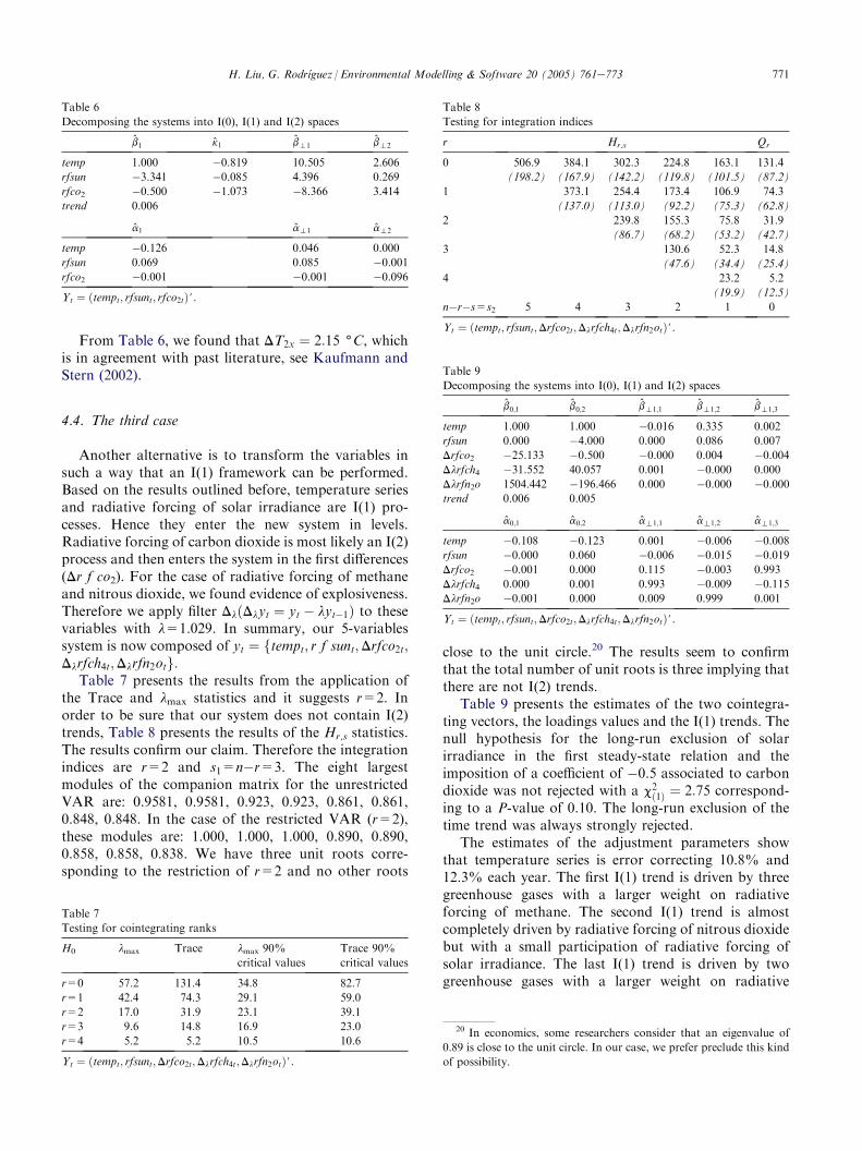
From Table 6, we found that DT2x ¼ 2:15 (C, whichis in agreement with past literature, see Kaufmann andStern (2002).

4.4. The third case

Another alternative is to transform the variables insuch a way that an I(1) framework can be performed.Based on the results outlined before, temperature seriesand radiative forcing of solar irradiance are I(1) pro-cesses. Hence they enter the new system in levels.Radiative forcing of carbon dioxide is most likely an I(2)process and then enters the system in the first differences(Dr f co2). For the case of radiative forcing of methaneand nitrous dioxide, we found evidence of explosiveness.Therefore we apply filter DlðDlyt ¼ yt � lyt�1Þ to thesevariables with l=1.029. In summary, our 5-variablessystem is now composed of yt ¼ ftempt; r f sunt;Drfco2t;Dlrfch4t;Dlrfn2otg:

Table 7 presents the results from the application ofthe Trace and lmax statistics and it suggests r=2. Inorder to be sure that our system does not contain I(2)trends, Table 8 presents the results of the Hr,s statistics.The results confirm our claim. Therefore the integrationindices are r=2 and s1=n�r=3. The eight largestmodules of the companion matrix for the unrestrictedVAR are: 0.9581, 0.9581, 0.923, 0.923, 0.861, 0.861,0.848, 0.848. In the case of the restricted VAR (r=2),these modules are: 1.000, 1.000, 1.000, 0.890, 0.890,0.858, 0.858, 0.838. We have three unit roots corre-sponding to the restriction of r=2 and no other roots

close to the unit circle.20 The results seem to confirmthat the total number of unit roots is three implying thatthere are not I(2) trends.

Table 9 presents the estimates of the two cointegra-ting vectors, the loadings values and the I(1) trends. Thenull hypothesis for the long-run exclusion of solarirradiance in the first steady-state relation and theimposition of a coefficient of �0.5 associated to carbondioxide was not rejected with a c2

ð1Þ ¼ 2:75 correspond-ing to a P-value of 0.10. The long-run exclusion of thetime trend was always strongly rejected.

The estimates of the adjustment parameters showthat temperature series is error correcting 10.8% and12.3% each year. The first I(1) trend is driven by threegreenhouse gases with a larger weight on radiativeforcing of methane. The second I(1) trend is almostcompletely driven by radiative forcing of nitrous dioxidebut with a small participation of radiative forcing ofsolar irradiance. The last I(1) trend is driven by twogreenhouse gases with a larger weight on radiative

Table 6

Decomposing the systems into I(0), I(1) and I(2) spaces

b1 k1 bt1 bt2

temp 1.000 �0.819 10.505 2.606

rfsun �3.341 �0.085 4.396 0.269

rfco2 �0.500 �1.073 �8.366 3.414

trend 0.006

a1 at1 at2

temp �0.126 0.046 0.000

rfsun 0.069 0.085 �0.001

rfco2 �0.001 �0.001 �0.096

Yt ¼ ðtempt; rfsunt; rfco2tÞ#.

Table 7



critical values

Trace 90%

critical values

r=0 57.2 131.4 34.8 82.7

r=1 42.4 74.3 29.1 59.0

r=2 17.0 31.9 23.1 39.1

r=3 9.6 14.8 16.9 23.0

r=4 5.2 5.2 10.5 10.6

Yt ¼ ðtempt; rfsunt;Drfco2t;Dlrfch4t;Dlrfn2otÞ#.

Table 8


r Hr,s Qr

0 506.9 384.1 302.3 224.8 163.1 131.4

(198.2) (167.9) (142.2) (119.8) (101.5) (87.2)

1 373.1 254.4 173.4 106.9 74.3

(137.0) (113.0) (92.2) (75.3) (62.8)

2 239.8 155.3 75.8 31.9

(86.7) (68.2) (53.2) (42.7)

3 130.6 52.3 14.8

(47.6) (34.4) (25.4)

4 23.2 5.2

(19.9) (12.5)

n�r�s=s2 5 4 3 2 1 0


Table 9

Decomposing the systems into I(0), I(1) and I(2) spaces

b0;1 b0;2 bt1;1 bt1;2 bt1;3

temp 1.000 1.000 �0.016 0.335 0.002

rfsun 0.000 �4.000 0.000 0.086 0.007

Drfco2 �25.133 �0.500 �0.000 0.004 �0.004

Dlrfch4 �31.552 40.057 0.001 �0.000 0.000

Dlrfn2o 1504.442 �196.466 0.000 �0.000 �0.000

trend 0.006 0.005

a0;1 a0;2 at1;1 at1;2 at1;3

temp �0.108 �0.123 0.001 �0.006 �0.008

rfsun �0.000 0.060 �0.006 �0.015 �0.019

Drfco2 �0.001 0.000 0.115 �0.003 0.993

Dlrfch4 0.000 0.001 0.993 �0.009 �0.115

Dlrfn2o �0.001 0.000 0.009 0.999 0.001


20 In economics, some researchers consider that an eigenvalue of

0.89 is close to the unit circle. In our case, we prefer preclude this kind

of possibility.


forcing carbon dioxide and again, a small participationof radiative forcing of solar irradiance.

5. Conclusions

This paper applies multivariate I(1) and I(2) tools toidentify for the existence and the number of long-runsteady-state relations between temperature series andradiative forcing of solar radiance and a set of threegreenhouse gases. One of the results indicate thattemperature and radiative forcing of solar irradianceseries appear to be I(1) processes, radiative forcing ofcarbon dioxide is an I(2) process, and radiative forcingof methane and nitrous dioxide seem to containexplosive roots. In most variables (temperature, radia-tive forcing of solar irradiance and carbon dioxide), ourresults confirm previous evidence in the literature.

Given the complex structure and properties of the timeseries, we analyzed three alternative cases. In the firstcase, a 5-variable system is considered. The second caseconsisted of variables with I(1) and I(2) characteristicsand the ones with explosive behavior separately. The lastsystem considers a transformation of the variables in sucha way that the I(1) framework can be used. Overall, allsystems show that temperature series is error correctingthe disequilibria towards the static steady-state ordynamic steady-state relations. The degree of adjustmentof the temperature depends on which cointegratingrelations is considered but it goes from 5% to 65%. Thehigher rates of adjustment are comparable to the resultsfound by Stern and Kaufmann (2000). In some cases,however, temperature series is not error correcting for thelong-run disequilibria. It means that there is nothing inthe system (the earth and its components) that allows forcorrecting these disequilibria. On the other hand, thehigher rates of adjustment respect to other disequilibriacould suggest abrupt changes in temperature in order tocorrect for these disequilibria.

Another interesting result is the composition of theI(1) and I(2) trends. According to our results, bothtrends are essentially composed by a linear combinationof greenhouse gases that are affecting the temperatureseries strongly. In an specific case, we find that the I(1)trend is driven by temperature and radiative forcing ofsolar irradiance, whereas the I(2) trend is driven bya linear combination of the three greenhouse gases orexclusively by the radiative forcing of carbon dioxide.The first component could be associated to inertial and/or natural factors. In the case of the second component,it could be related to human factors.

Finally, we find that the equilibrium temperaturechange for a doubling of carbon dioxide is between 2.15and 3.4 (C, which is agreement with previous literatureand the report of the IPCC (2001) using 15 differentgeneral circulation models.

Acknowledgements

An earlier version of this paper has benefited fromuseful comments from the participants to the 35thAnnual Conference of the Canadian Economic Associ-ation, Calgary, 2001. We thank constructive commentsfrom two referees and the Editor. The writing of thispaper was finished while G.R. was visiting the School ofEconomics of the University of New South Wales,Australia, and he thanks particularly Garry Barret.Financial support from the Faculty of Social Sciences isacknowledged.

References

Bloomfield, P., 1992. Trends in global temperature. Climatic Change

21, 1e16.

Bloomfield, P., Nychka, D., 1992. Climate spectra and detecting

climate change. Climatic Change 21, 275e287.

Dickey, D.A., Fuller, W.A., 1979. Distribution of the estimators for

autoregressive time series with a unit root. Journal of the American

Statistical Association 74, 427e431.

Dickey, D.A., Pantula, S.G., 1987. Determining the order of differ-

encing in autoregressive process. Journal of Business and Economic

Statistics 5, 455e461.

Doornik, D.A., Hendry, D.F., 2001. Modelling Dynamic Systems

Using PcGive 10.0, vol. II. Timberlake Consultants, UK.

Elliott, G., Rothenberg, T., Stock, J.H., 1996. Efficient tests for an

autoregressive unit root. Econometrica 64, 813e839.

Fiess, N., MacDonald, R., 2001. The instability of the money demand

function: an I(2) interpretation. Oxford Bulletin of Economics and

Statistics 63 (4), 475e495.Fomby, T., Vogelsang, T., 2002. Application of size robust trend

analysis to global warming temperature series. Journal of Climate

15, 117e123.Galbraith, J.W., Green, C., 1993. Inference about trend in global

temperature data. Climatic Change 22, 209e221.

Haldrup, N., 1999. A review of the econometric analysis of I(2)

variables. In: Oxley, L., McAleer, M. (Eds.), Practical Issues in

Cointegration Analysis. Blackwell, Oxford.

Haldrup, N., Lildholdt, P., 2002. On the robustness of unit root tests in

the presence of double unit roots. Journal of Time Series Analysis

23 (2), 155e171.Hansen, H., Juselius, K., 1995. CATS in RATS, Manual to

Cointegration Analysis of Time Series. Estima, Evanston, IL.

Harvey, A.C., 1989. Forecasting, Structural Time Series Models, and

the Kalman Filter. Cambridge University Press.

Hasza, D.P., Fuller, W.A., 1979. Estimation of autoregressive

processes with unit roots. Annals of Statistics 7, 1106e1120.

Holtemoller, O., 2002. Money and Prices: An I(2) Analysis for the

Euro Area. Working Paper. Humboldt-Universitat, Berlin.

IPCC (Intergovernmental Panel on Climate Change). 2001. In:

Houghton, J.T., Ding, Y., Griggs, D.J. (Eds.), Climate Change

2001: the Intergovernmental Panel on Climate Change Scientific

Assessment. Cambridge University Press, Cambridge, UK, New

York, NY, USA, pp. 358.

Johansen, S., 1988. Statistical analysis of cointegration vectors.

Journal of Economic Dynamics and Control 12, 231e254.Johansen, S., 1992. A representation of vector autoregressive process

of order 2. Econometric Theory 8, 188e202.

Johansen, S., 1995a. A statistical analysis of cointegration for I(2)

variables. Econometric Theory 11, 25e59.


Johansen, S., 1995b. Likelihood-Based Inference in Cointegrated

Vector Autoregressive Models. Oxford University Press, Oxford.

Johansen, S., Juselius, K., 1992. Testing structural hypothesis in

a multivariate cointegration analysis of the PPP and the UIP for

UK. Journal of Econometrics 53, 211e244.Johansen, S., Juselius, K., 1994. Identification of the long-run and the

short-run structure. An application to the ISLM Model. Journal of

Econometrics 63, 7e36.Juselius, K., 1999. Price convergence in the medium and long run: an

I(2) analysis of six price indices. In: Engle, R.F., White, H. (Eds.),

Cointegration, Causality and Forecasting (A Festschrift in Honour

of Clive W.J. Granger). Oxford University Press, New York.

Juselius, K., 2003. Inflation, money growth, and I(2) analysis.

Unpublished manuscript.

Kaufmann, A., Stern, D.I., 1997. Evidence for human influence on

climate from hemispheric temperature relations. Nature 388, 39e44.Kaufmann, A., Stern, D.I., 2002. Cointegration analysis of hemi-

spheric temperature relations. Journal of Geophysical Research

107 (D2), 10.1029/2000JD000174.

Kelly, D.L., 2000. Unit Roots in the Climate: Is the Recent Warming

Due to Persistent Shocks? Working Paper. Department of Eco-

nomics, University of Miami.

Kuo, C., Lindberg, C., Thompson, D.J., 1990. Coherence established

between atmospheric carbon dioxide and global temperature.

Nature 388, 39e44.

Kongsted, H.C., 2003. An I(2) Cointegration Analysis of Small-

Country Import Price Determination. Institute of Economics,

University of Copenhagen.

Lean, J., Beer, J., Bradley, R., 1995. Reconstruction of solar irradiance

since 1610: implications for climate change. Geophysical Research

Letters 22, 3195e3198.

Lenten, L.J.A., Moosa, I.A., 2003. An empirical investigation into

long-term climate change in Australia. Environmental Modelling &

Software 18, 59e70.Nielsen, B., 2001. The Asymptotic distribution of unit root tests of

unstable autoregressive processes. Econometrica 69, 211e219.

Nielsen, B., 2002. Cointegration Analysis of Explosive Processes.

Discussion Paper. Nuffield College, Oxford.

Paruolo, P., 1996. On the determination of integration indices in I(2)

systems. Journal of Econometrics 72, 313e356.

Paruolo, P., Rahbek, A., 1999. Weak exogeneity in I(2) VAR systems.

Journal of Econometrics 93, 281e308.Phillips, P.C.B., Perron, P., 1988. Testing for a unit root in time series

regression. Biometrika 75, 335e346.

Rahbek, A., Kongsted, H.C., Jorgensen, C., 1999. Trend stationarity

in the I(2) cointegration model. Journal of Econometrics 90,

265e289.

Richards, G.R., 1993. Change in global temperature: a statistical

analysis. Journal of Climate 6, 546e559.

Said, E.S., Dickey, D.A., 1984. Testing for unit roots in autoregressive-

moving average models of unknown order. Biometrika 71,

599e607.

Santer, B.D., Taylor, K.E., Wigley, T.M.L., Johns, T.C., Jones, P.D.,

Karoly, D.J., Mitchell, J.F.N., Oort, A.H., Penner, J.E., Ram-

aswamy, V., Schwartzkopf, M.D., Stouffer, R.J., Tett, S., 1996. A

search for human influences on the thermal structure of the

atmosphere. Nature 382, 39e46.

Schmidt, P., Phillips, P.C.B., 1992. LM tests for a unit root in the

presence of deterministic trends. Oxford Bulletin of Economics and

Statistics 54, 257e287.

Schonwiese, C.-D., 1994. Analysis and prediction of global climate

temperature change based on multiforced observational statistics.

Environmental Pollution 83, 149e154.Stern, D.I., Kaufmann, R.K., 1997. Time Series Properties of Global

Climate Variables: Detection and Attribution of Climate Change.

Working Paper in Ecological Economics, 9702. Center for

Resource and Environmental Studies, Australian National Uni-

versity.

Stern, D.I., Kaufmann, R.K., 1999. Econometric analysis of global

climate change. Environmental Modelling & Software 14,

597e605.

Stern, D.I., Kaufmann, R.K., 2000. Detecting a global warming signal

in hemispheric temperature series: a structural time series analysis.

Climatic Change 47, 411e438.Stock, J.H., Watson, M.W., 1998. Testing for common trends. Journal

of the American Statistical Association 83, 1097e1107.

Tol, R.S., DS, J., 1994. Greenhouse statistics-time series analysis: part

II. Theoretical and Applied Climatology 49, 63e74.

Tol, R.S., de Vos, A.F., 1998. A Bayesian statistical analysis of the

enhanced greenhouse effect. Climatic Change 38, 87e112.

Thomson, D.J., 1995. The seasons, global temperature, and precession.

Science 268, 59e68.

Thomson, D.J., 1997. Dependence of global temperatures on

atmospheric CO2 and solar irradiance. Proceedings of the National

Academy of Sciences USA 94, 8370e8377.Vostroknutova, E., 2003. Shock Therapy? An I(2) Cointegration

Analysis of the Russian Stabilization. EUI Working Paper ECO,

No. 2003/16. Department of Economics, European University

Institute.

Woodward, W.A., Gray, H.L., 1993. Global warming and the problem

of testing for trend in time series data. Journal of Climate 6,

953e962.

Woodward, W.A., Gray, H.L., 1995. Selecting a model for detecting

the presence of a trend. Journal of Climate 8, 1929e1937.


Human activities and global warming: a cointegration analysis

Documents

Transcript of Human activities and global warming: a cointegration analysis