15

Mr. SHARP. Thank you very much, Dr. Firor. We are going to

take a break for probably 10 or 15 minutes as we go over to vote

and come back and then we will be happy to hear from our other

two witnesses before we have questions for the panel.

Thank you .

[ Brief recess.]

Mr. SHARP. Thank you very much for your patience with the

House schedule. Dr. Hansen, we'll be very pleased to hear from you

at this point. We were just discussing duringthe break how we can

start solving problems. We're not that good, I'm afraid .

STATEMENT OF JAMES E. HANSEN

Mr. HANSEN. Thank you for the opportunity to testify today on

the greenhouse effect, or, as I sometimes call it , the hothouse

effect.

My testimony today is based in large part on research carried

out with my colleagues at the NASA Goddard Institute for Space

Studies , which is located at Columbia University in New York City.

Before I present our results, I'd like to state that the fact that

NASA has approvedpresentation of our scientific research results,

does not imply that NASA has taken a policy position with regard

to the greenhouse effect.

Also, I would like to point out that our scientific results are

recent. Some are still in press or in preparation and we do not

expect every scientist to agree with all of our results. I will address

questions of scientific uncertainty in my remremarks.

My principal conclusions are; number one, the earth is presently

warmer than at any time in the history of instrumental measure

ments. Number two, the greenhouse effect is probably the principal

cause of the current global warmth . Number three , our computer

climate simulations suggest that the greenhouse effect is already

large enough to begin to affect the probability of extreme events

such as summer heat waves.

[Slide]

Mr. HANSEN. My first conclusion is illustrated by the first Vu

Graph which shows the global temperature over the period of in

strumental records, which is about 100 hundred years — based on

measurements at about 2,000 meteorological stations located

around the world . The present temperature is the highest in this

period of record. The rate of warming in the past 25 years is the

highest on record. During 1988, so far, is so much warmer than

1987, that barring an improbable cooling during the rest of the

year, 1988 will be the warmest year on record . The 5 warmest

years, counting 1988, all occurred in the 1980's. So there's no real

doubt or scientific dispute that the earth is getting warmer at a

rapid rate .

My second conclusion isthat the greenhouse effect is probably

the principal cause of the global warming. This conclusion requires,

first, that the observed warming be larger than natural climate

variability and, second, that the magnitude and nature of the

warmingbe consistent with the greenhouse mechanism .

These are difficult and complicated issues and yet they are

simple, because the simple fact of the matter is that the earth in

16

the past 25-30 years has warmed by an amount which is three

times larger than the magnitude of the typical natural climate

fluctuation. We can therefore state with a high degree of confi

dence, that it is a real warming trend - not a chance fluctuation.

In my opinion, we can say this with about 99 percent confidence,

but I'm aware that there are questions about exactly how you

define that confidence. It may be better if I simply state that it is a

high degree of confidence and thereby avoid discussion with some

of mycolleagues, which discussion can simply confuse the issue.

Now , the second half of the problem : are the magnitude and nature

of the observed warming consistent with the greenhouse mecha

nism ?

Again , this is a complex issue and we don't have time for details

here. The simple answer is, yes, the magnitude and trend of the

global temperature rise are similar to what is expected and com

puted for the greenhouse effect and so is the next level of detail in

the climate change — the spatial and seasonal distribution of the

warming.

All together, the evidence that the earth is warming by an

amount which is too large to be a chance fluctuation and the simi

larity of the warming to that expected from the greenhouse effect,

represent a very strong case, in my opinion , that the greenhouse

effect has been detected and is changing our climate now.

My third conclusion concerns the impact of the greenhouse effect

on the likelihood and the severity of heat wave drought situations .

We have used our global climate model for numerical simulations

of the greenhouse effect on a large computer. These climate models

are not yet sufficiently realistic to reliably simulate regional cli

mate patterns, but they can give us an indication of the magnitude

of expected greenhouse climate changes and how these compare to

natural climate fluctuations.

What we find is that the greenhouse effect, as yet, is quite a bit

smaller than the natural fluctuations of climate which occur from

year to year at a given place. So, please don't call me next season if

it's cold in Indiana, and tell me that the greenhouse theory is

wrong, because that's not an inference which you could make.

What our climate models do show, is that the greenhouse effect is

reaching a magnitude now where it can have a noticeable impact

on the probability of a warmseason .

This die here, represents the probability of having a hot summer

during the period 1950-1980. The Weather Bureau defines the one

third hottest summers during that period as hot - simply as a defi

nition as to what “ hot ” is ata given locality. So the probability of a

hot summer is represented by having two out of the six diefaces

colored red. Similarly, the probability of having a cold summer, by

their definition , is the one third coldest summers during the period

1950-1980. We represent that by the blue sides on the die face. The

typical or average conditions are represented by the white sides.

By 1995, which is 7 years in the future, we calculate that the

greenhouse effect has changed the probabilities such that four sides

of the die are red. One side is white for conditions average for 1950

1980, and one side is blue, or colder than average 1950-1980 condi

tions. So one thing you can say is, that even in the 1990's, with the

expected increased greenhouse effect, there are going to be some

17

years which are colder than normal - probably about 2 years

during the 1990's.

The main thing I want to say from this, is that it's my opinion

that at least by 1995, the manin the street is going to notice this

change in the probabilities. He is going to say, what's going on

here? This die is loaded. We're having hot summers more often

than we used to and the hottest ones are hotter than they used to

be.

Of course, one thing that concerns me is that when we get to this

point, the man in the street, who's also the voter in the booth , is

going to say, why didn't you scientists and Congressmen warn us

about this and maybe even consider doing something about it ? I'm

afraid that perhaps all that we'll be able to say is, well, we did

think aboutit one hot summer in 1988, but there were scientific

uncertainties and we couldn't figure them out exactly and the next

season wasn't so hot, so we didn't have 100 percent confidence and

we were afraid to risk our reputations, et cetera.

Now , with regard to the drought, let me say that there is strong

scientific evidence that the large greenhouse effect that is expected

several decades in the future, if green house gases continue to in

crease at recent rates, that this will cause a significant increase in

the frequency and the severity of heat wave/drought situations in

mid -latitude ,continental regions such asthe United States.

Moreover, the climate simulations that we've done with our

model at the Goddard Institute suggest that the greenhouse effect

in the late 1980's and in the 1990'sis already large enough to in

crease the likelihood of heat wave /drought situations in the south

east and the Midwest United States, even though it is inappropri

ate to blame a specific drought on the greenhouse effect.

My written testimony, the same as the testimony I gave at the

Senate a couple weeks ago , contains further discussion of that

topic. I would like to finish by making a few brief recommenda

tions, if the chairman will allow.

Mr. SHARP. I would be happy to .

Mr. HANSEN . These are the personal opinions of Jim Hansen ,

Ridgewood, NJ. I have not attempted to get official approval of

them .

Number one, I think we have to provide more support for stu

dents and post-doctoral researchers in the global climate area.

When we get to this point in the 1990's, when the man in the

street can see that theclimate is, in fact, changing, we had better

have the brain power to begin to understand the climate system ,

to understand the system and some of the implications of that

changing climate. Right now , it seems to me the best students are

going into law school, into medical school, and we need to be able

to attract some of the best students into this area .

Number two, we need to have global observations to understand

the climate. That means observationsfrom space, from the ground,

and within the oceans. The data need to be collected over a suffi

ciently long time period; so we need to get started soon.

Numberthree, my final recommendation , I think we could take

some steps now to reduce the rate of growth of the greenhouse

effect. Chlorofluorocarbons, which destroy ozone as well as cause 20

percent of the greenhouse effect, could be phased out entirely over

18

an appropriate period of time. The manufactures agree that there

are orwill be substitutes for the chlorofluorocarbons.

Also, we should increase our energy efficiency, because CO2

causes 55-60 percent of the greenhouseeffect. There's a lot of room

for improved efficiency. It would have other benefits, independent

of thegreenhouse effect, especially on our balance of payments def

icit. How to get at that problem is, of course , a major difficulty and

that's something you can address better than I can. I know that

there are majorways that we could improve our energy efficiency.

Finally, I think we should discourage deforestation and encour

age reforestation, because that would not only reduce atmosphere

CO2, but also preserve the habitat for innumerable, valuable biolog

ical species. The impact of these kinds of steps on the short run is

going to be relatively small, but it's very important, because it

would change the direction in which the greenhouse effect is

headed . Instead of the sharp, upward ramp that we're on now , it

could put us on a more manageable course on the longer term , over

the next several decades. Thank you.

[Testimony resumes on p. 53.]

[ The prepared statement of Mr. Hansen follows:]

19

STATEMENT OF

James E. Hansen

NASA Goddard Institute for Space Studies

2880 Broadway , New York , N.Y. 10025

PREFACE

This statement is based largely on recent studies carried out with my

colleagues S. Lebedeff , D. Rind , I. Fung , A. Lacis , R. Ruedy , G. Russell and

P. Stone at the NASA Goddard Institute for Space Studies .

My principal conclusions are : ( 1 ) the earth is warmer in 1988 than at any

time in the history of instrumental measurements , ( 2 ) the global warming is now

sufficiently large that we can ascribe with a high degree of confidence a cause

and effect relationship to the greenhouse effect , and ( 3 ) in our computer climate

simulations, the greenhouse effect now is already large enough to begin to affect

the probability of occurrence of extreme events such as summer heat waves ; the

model results imply that heat wave / drought occurrences in the Southeast and

Midwest United States may be more frequent in the next decade than in

climatological ( 1950-1980 ) statistics .

1. Current global temperatures

Present global temperatures are the highest in the period of instrumental

records , as shown in Fig . 1. The rate of global warming in the past two decades

is higher than at any earlier time in the record . The four warmest years in the

past century all have occurred in the 1980's .

The global temperature in 1988 up to June 1 is substantially warmer than the

like period in any previous year in the record . This is illustrated in Fig . 2 ,

which shows seasonal temperature anomalies for the past few decades . The most

recent two seasons ( Dec. - Jan . - Feb. and Mar. - Apr. -May , 1988 ) are the warmest in

the entire record . The first five months of 1988 are so warm globally that we

conclude that 1988 will be the warmest year on record unless there is a

remarkable , improbable cooling in the remainder of the year .

2. Relationship of global warming and greenhouse effect

Causal association of current global warming with the greenhouse effect

requires determination that ( 1 ) the warming is larger than natural climate

variability , and ( 2 ) the magnitude and nature of the warming is consistent with

the greenhouse warming mechanism . Both of these issues are addressed

quantitatively in Fig . 3 , which compares recent observed global temperature

change with climate model simulations of temperature changes expected to result

from the greenhouse effect .

The present observed global warming is close to 0.4 ° C , relative to

' climatology ', which is defined as the thirty year ( 1951-1980 ) mean . A warming

of 0.4 ° C is three times larger than the standard deviation of annual mean

temperatures in the 30 -year climatology . The standard deviation of 0.13ºC is a

typical amount by which the global temperature fluctuates annually about its 30

year mean ; the probability of a chance warming of three standard deviations is

about 1% . Thus we can state with about 99 % confidence that current temperatures

represent a real warming trend rather than a chance fluctuation over the 30 year

period .

20

3

We have made computer simulations of the greenhouse effect for the period

since 1958 , when atmospheric CO2 began to be measured accurately . A range of

trace gas scenarios is considered so as to account for moderate uncertainties in

trace gas histories and larger uncertainties in future trace gas growth rates .

The nature of the numerical climate model used for these simulations is described

in attachment A ( reference 1 ) . There are major uncertainties in the model , which

arise especially from assumptions about ( 1 ) global climate sensitivity and ( 2 )

heat uptake and transport by the ocean , as discussed in attachment A. However ,

the magnitude of temperature changes computed with our climate model in various

test cases is generally consistent with a body of empirical evidence ( reference

2 ) and with sensitivities of other climate models ( reference 1 ) .

The global temperature change simulated by the model yields a warming over

the past 30 years similar in magnitude to the observed warming ( Fig . 3 ) . In both

the observations and model the warming is close to 0.4 ° C by 1987 , which is the

99 % confidence level .

It is important to compare the spatial distribution of observed temperature

changes with computer model simulations of the greenhouse effect , and also to

search for other global changes related to the greenhouse effect , for example ,

changes in ocean heat content and sea ice coverage . As yet , it is difficult to

obtain definitive conclusions from such comparisons , in part because the natural

variability of regional temperatures is much larger than that of global mean

temperature . However , the climate model simulations indicate that certain gross

characteristics of the greenhouse warming should begin to appear soon , for

example, somewhat greater warming at high latitudes than at low latitudes ,

greater warming over continents than over oceáns , ' and cooling in the stratosphere

while the troposphere warms . Indeed , observations contain evidence for all these

characteristics , but much more study and improved records are needed to establish

the significance of trends and to use the spatial information to understand

better the greenhouse effect . Analyses must account for the fact that there are

climate change mechanisms at work , besides the greenhouse effect ; other anthropo

genic effects , such as changes in surface albedo and tropospheric aerosols , are

likely to be especially important in the Northern Hemisphere .

We can also examine the greenhouse warming over the full period for which

global temperature change has been measured , which is approximately the past 100

years . On such a longer period the natural variability of global temperature is

larger ; the standard deviation of global temperature for the past century is

0.2 ° C . The observed warming over the past century is about 0.6-0.7 ° C . Simulated

greenhouse warming for the past century is in the range 0.5 ° -1.0 ° C , depending

upon various modeling assumptions ( e.g. , reference 2 ) . Thus , although there are

greater uncertainties about climate forcings in the past century than in the past

30 years , the observed and simulated greenhouse warmings are consistent on both

of these time scales .

Conclusion . Global warming has reached a level such that we can ascribe

with a high degree of confidence a cause and effect relationship between the

greenhouse effect and the observed warming . Certainly further study of this

issue must be made . The detection of a global greenhouse signal represents only

a first step in analysis of the phenomenon .

21

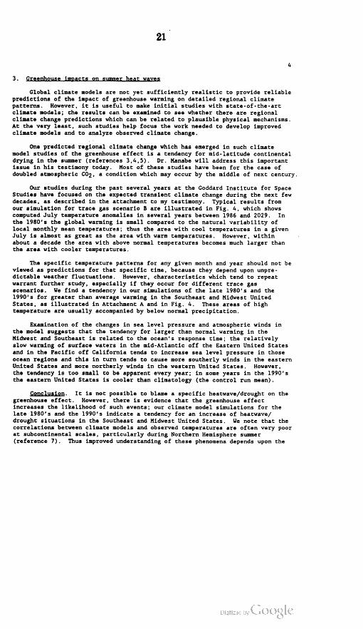
3 . Greenhouse impacts on summer heat waves

Global climate models are not yet sufficiently realistic to provide reliable

predictions of the impact of greenhouse warming on detailed regional climate

patterns . However , it is useful to make initial studies with state - of - the - art

climate models ; the results can be examined to see whether there are regional

climate change predictions which can be related to plausible physical mechanisms .

At the very least , such studies help focus the work needed to develop improved

climate models and to analyze observed climate change .

One predicted regional climate change which has emerged in such climate

model studies of the greenhouse effect is a tendency for mid - latitude continental

drying in the summer ( references 3,4,5 ) . Dr. Manabe will address this important

issue in his testimony today . Most of these studies have been for the case of

doubled atmospheric CO2 , a condition which may occur by the middle of next century .

Our studies during the past several years at the Goddard Institute for Space

Studies have focused on the expected transient climate change during the next few

decades , as described in the attachment to my testimony . Typical results from

our simulation for trace gas scenario B are illustrated in Fig . 4 , which shows

computed July temperature anomalies in several years between 1986 and 2029. In

the 1980's the global warming is small compared to the natural variability of

local monthly mean temperatures; thus the area with cool temperatures in a given

July is almost as great as the area with warm temperatures . However , within

about a decade the area with above normal temperatures becomes much larger than

the area with cooler temperatures .

The specific temperature patterns for any given month and year should not be

viewed as predictions for that specific time , because they depend upon unpre

dictable weather fluctuations . However , characteristics which tend to repeat

warrant further study , especially if they occur for different trace gas

scenarios . We find a tendency in our simulations of the late 1980's and the

1990's for greater than average warming in the Southeast and Midwest United

States , as illustrated in Attachment A and in Fig . 4 . These areas of high

temperature are usually accompanied by below normal precipitation .

Examination of the changes in sea level pressure and atmospheric winds in

the model suggests that the tendency for larger than normal warming in the

Midwest and Southeast is related to the ocean's response time ; the relatively

slow warming of surface waters in the mid -Atlantic off the Eastern United States

and in the Pacific off California tends to increase sea level pressure in those

ocean regions and this in turn tends to cause more southerly winds in the eastern

United States and more northerly winds in the western United States . However ,

the tendency is too small to be apparent every year ; in some years in the 1990's

the eastern United States is cooler than climatology ( the control run mean) .

Conclusion It is not possible to blame a specific heatwave /drought on the

greenhouse effect . However , there is evidence that the greenhouse effect

increases the likelihood of such events ; our climate model simulations for the

late 1980's and the 1990's indicate a tendency for an increase of heatwave/

drought situations in the Southeast and Midwest United States . We note that the

correlations between climate models and observed temperatures are often very poor

at subcontinental scales , particularly during Northern Hemisphere summer

( reference 7 ) . Thus improved understanding of these phenomena depends upon the

22

development of increasingly realistic global climate models and upon the

availability of global observations needed to verify and improve the models .

REFERENCES

1 . Hansen J. , I. Fung, A. Lacis , D. Rind , G. Russell , S. Lebedeff , R. Ruedy and

P. Stone , 1988 , Global climate changes as forecast by the GISS 3 - D model ,

J. Geophys . Res . ( in press ) .

Hansen , J. , A. Lacis , D. Rind , G. Russell , P. Stone , I. Fung , R. Ruedy and

J. Lerner , 1984 , Climate sensitivity : analysis of feedback mechanisms ,

Geophys . Mono . , 29 , 130-163 .

3. Manabe , S. , R. T. Wetherald and R. J. Stauffer , 1981 , Summer dryness due to

an increase in atmospheric CO2 concentration , Climate Change , 3 , 347-386 .

4 . Manabe , S. and R. T. Wetherald , 1986 , Reduction in summer soil wetness in

duced by an increase in atmospheric carbon dioxide , Science , 232 , 626-628 .

5. Manabe , S. and R. T. Wetherald , 1987 , Large - scale changes of soil wetness

induced by an increase in atmospheric carbon dioxide , J. Atmos . Sci . , 44 ,

1211-1235 .

6. Hansen , J. and s . Lebedeff, 1987 , Global trends of measured surface air

temperature, J. Geophy's . Res. , 92 , 13,345-13,372 ; Hansen , J. and s .

Lebedeff , 1988 , Global surface air temperatures : update through 1987 ,

Geophys . Res . Lett . , 15 , 323-326 .

Grotch , s . , 1988 , Regional intercomparisons of general circulation model

predictions and historical climate data , Dept. of Energy Report ,

DOE /NBA - 0084 .

23

GLOBAL TEMPERATURE TREND0.6

(5 months)Annual Mean

5 Year Running Meono

0.2

........

O

AT

(°C)

m

n-0.2

-0.4 %

tw

I Error Estimates (95% Confidence)

-0.6

-0.8

1880 1900 1920 1940 1960 1980 1990

DATE

Fig . 1. Global surface air temperature change for the past century , with the

zero point defined as the 1951-1980 nean . Uncertainty bars ( 95$ confidence

limits) are based on an error analysis as described in reference 6 ; inner bars

refer to the 5 -year nean and outer bars to the annual mean . The analyzed un

certainty is a result of incomplete spatial coverage by measurement stations,

primarily in ocean areas . The 1988 point compares the January -May 1988 tempera

ture to the nean for the same 5 months in 1951-1980 .

Global Temperature Change

0.6

0.4

....

::::::::**0.3

0.2 nos

----

AT

(°C) ........

....... fronter

:

O

***.........

ind

Looms

::.........

-0.2

Limit

:11111

-0.4

1958 1965 1980 1985 19881970 1975

Date

Fig . 2. Global surface air temperature change at seasonal resolution for the

past 30 years . Figures 1 and 2 are updates of results in reference 6 .

24

1.5 Annual Mean Global Temperature Change

Estimated Temperatures During

Altithermal and Eemian Times

1.0

AT

(° C )

8

0.5

0%

.OBSERVED

SCENARIO A

SCENARIO B

SCENARIO C.

-0.4v

1960

V

1970

v

1980

v

1990

Date

V

2000 2010

V

2019

Fig . 3. Annual mean global surface air temperature computed for trace gas scenarios

A , B and C described in reference 1. ( Scenario A assumes continued growth rates of

trace gas emissions typical of the past 20 years, i.e. , about 1.58 yr emission

growth ; scenario B has emission rates approximately fixed at current rates ; scenario

c drastically reduces trace gas emissions between 1990 and 2000. ) Observed

temperatures are from reference 6. The shaded range is an estimate of global

temperature during the peak of the current and previous interglacial periods , about

6,000 and 120,000 years before present , respectively . The zero point for

observations is the 1951-1980 mean (reference 6 ) ; the zero point for the model is

the control run mean .

!

25

SCENARIO

B

JULY

1986

ME

AN

AT

:+0.6

°CME

ANAT

:+0.2

°C90

JULY

2000

60

30

0 -30 -60

-90

MEAN

AT

:+0.3

°C90

JULY

1987

ME

ANAT

:+1.0

°CJULY

2015

Z조

60

30 30

-90

MEAN

AT

:+0.5

°C90

JULY

1990

MEAN

AT

:+ 1.5

°CJULY

2029

30 -30

-60

.90 -180

-120

-60

60

120

180

-100

-120

-60

O60

120

180

ATI

°c)

-2

2

Fig

.4.Simulated

July

surface

air

temperature

anomalies

for

six

individual

years

of

scenario

B,

compared

toa100

year

control

run

with

1958

atmospheric

composition

(see

Attachment

A).

26

ATTACHMENT A

Global Climate Changes as Forecast by Goddard Institute for Space Studies

Three -Dimensional Model

J. HANSEN, I. FUNG, A. LACIS, D. RIND, S. LEBEDEFF, R. RUEDY, AND G. RUSSELL

NASA Goddard Space Flighe Cenier, Goddard Institutefor Space Studies, New York

P. STONE

Massachusetts Institute ofTechnology, Cambridge

We use a three -dimensional climate model, the Goddard Institute for Space Studies (GISS) model II

with 8 by 10 horizontal resolution , to simulatethe global climate effectsof time-dependent variations

of atmospheric trace gases and aerosols. Horizontal heat transport by the ocean is fixed at valuesestimated for today's climate, and the uptake of heat perturbations by the ocean bencath the mixed

layer is approximated as vertical diffusion. We make a 100-year control run and perform experiments

for three scenarios of atmospheric composition. These experiments begin in 1988 and include measured

or estimated changes in atmospheric Co., CH , N , O , chlorofluorocarbons ( CFCs) and stratospheric

aerosols for the period from 1958 to the present. Scenario A assumes continued exponential trace gas

growth, scenario B assumes a reduced linear growth of trace gases, and scenario C assumes a rapid

cunailment of trace gas emissions such that the net climate forcing ceases to increase after the year

2000. Principal results from the experiments are as follows: (1) Global warming to the level attained at

the peak of the current interglacial and the previous interglacial occurs in all three scenarios; however,

there are dramatic differences in the levels of future warming, depending on trace gas growth. (2 ) The

greenhouse warmingshould be clearly identifiable in the 1990s; the global warming within the nextseveral years is predicted to reach and maintain a level at least three standard deviations above the

climatology of the 1950s. (3 ) Regions where an unambiguous warming appears earliest are low - latitude

oceans, China and interior areas in Asia, and ocean areas near Antarctica and the north pole; aspects

of the spatial and temporal distribution of predicted warming are clearly model-dependent,implying the

possibility of model discrimination by the 1990s and thusimproved predictions, if appropriate

observations are acquired. ( 4 ) The temperature changes are sufficiently large to have major impacts on

people and other parts of the biosphere, as shown by computed changes in the frequency of extreme

events and by comparison with previous climate trends. (5 )The model results suggest some near - term

regional climate variations, despite the fixed ocean heat transpon which suppresses many possible

regional climate fluctuations, for example, during the late 1980s and in the 1990s there is a tendencyfor greater than average warming in the southeastem and central United States and relatively cooler

conditions or less than average warming in the westem United States and much of Europe. Principal

uncertainties in the predictions involve the equilibrium sensitivity of the model to climate forcing, the

assumptions regarding heat uptake and transport by the ocean , and the omission of other less -cenain

climate forcings.

To appear in the Journal of Geophysical Research .

27

1. INTRODUCTION

Studies of the climate impact of increasing atmospheric 5.2 examines the spatial distribution of predicted decadalCo , have been made by means of experiments with three temperature changes, and seation 53 examines short -term

dimensional (3D ) climate models in which the amount of Co , and local temperature changes. In section 6, we summarizewas instantaneously doubled or quadrupled, with the model the model predictions and discuss the principal caveats and

then integrated forward in time to a new steady state assumptions upon which the results depend.

(Manabe and Wetherald, 1975; Manabe and Stouffer, 1980; Our transient climate experiments were initiated in early

Hansen et al., 1984 ; Washington and Meehl, 1984; Wilson and 1983, being run as a background job on the GISS mainframeMitchell, 1987). These models all yield a large climate computer, a general-purpose machine (Amdahl V - 6 ) of mid

impact at equilibrium for doubled CO2, with global mean 1970s vintage. Results for scenario A were reported at a

warming of surface air between about 20 and 5 ° C . conference in June 1984 (Shands and Hoffman, 1987), and

However, observations show that CO , is increasing grad results from all scenarios were presented at several later

ually: its abundance was 315 parts per million by volume conferences.

(ppmv) in 1958 when Keeling initiated accurate measurements

and is now about 345 ppmy, with current mean annual 2. CLIMATE MODEL

increments of about 1.5 ppmv (Keeling et al ., 1982). Also The atmospheric component of the global climate model

there are at least two other known global radiative forcingswe employ is described and its abilities and limitations for

of comparable magnitude: growth of several other trace simulating today's climate are documented as model II

gases (Wang et al., 1976; Lacis et al., 1981; Ramanathan et(Hansen a al. ( 1983 ), hereafter referred to as paper 1) .

al ., 1985] and variations in stratospheric aerosols due to The model solves the simultaneous equations for conserva.volcanic eruptions (Lamb, 1970; Mitchell, 1970 ; Schneider and tion of energy, momentum , mass, and water vapor and theMoss, 1975; Pollack at al., 1976; Hansen et al., 1978, 1980; equation ofstate on a coarse grid with nine atmospheric

Robock, 1981). Still other radiative forcings, such as changes layers and horizontal resolution 8º latitude by 10° longitude.

of solar irradiance, tropospheric aerosols, and land surface The radiation calculation includes the radiatively significant

properties, may also be significant, but quantitative informa atmospheric gases, aerosols, and cloud panicles. Cloudtion is insufficient to define the trends of these forcings cover and height are computed, but cloud opacity is

over the past several decades.specified as a function of cloud type, altitude, and thick

In this paper we study the response of a 3D global ness. The diurnal and seasonal cycles are included. The

climate model to realistic rates of change of radiative ground hydrology and surface albedo depend upon the local

forcing mechanisms. The transient response of the climate vegetation. Snow depth is computed, and snow albedo

system on decadal time scales depends crucially on the includes effects of snow age and masking by vegetation.

response of the ocean, for which adequate understanding The equilibrium sensitivity of this model for doubled CO2

and dynamical models are not available. Our procedure is to (315 ppmv - 630 ppmu) is 4.2° C for global mean surface air

use simple assumptions about ocean heat transport. Specifi- temperature (Hansen etal. (1984), hereafter referred to as

cally we assume that during the next few decades the rate paper 2 ). This is within, but near the upper end of, theand pattern of horizontal ocean heat transport will remain range 30 1.5 ° C estimated for climate sensitivity by

unchanged and the rate of heat uptake by the ocean National Academy of Sciences committees (Chamey, 1979 ;beneath the mixed layer can be approximated by diffusive Smagorinsky, 1982 ), where their range is a subjeative

mixing of heat perturbations. This "surprise -free" represen- estimate of the uncertainty based on climate-modeling

tation of the ocean provides a first estimate of the global studies and empirical evidence for climate sensitivity. The

transient climate response which can be compared both to sensitivity of our model is near the middle of the range

observations and to future simulations developed with aobtained in recent studies with general circulation models

dynamically interactive ocean . We include in this paper a . (GCMs) (Washington and Mechl, 1984; paper 2,1984; Manabe

description of the experiments and an analysis of computed andWetherald,1987; Wilson and Mitchell, 1987).

temperature changes; other computed quantities, such as Ocean temperature and ice cover were specified climatolchanges in the atmospheric generalcirculation, precipitation, ogically in the versionof model II documented in paper 1 .

and sea ice cover will be presented elsewhere.In the experiments described here and in paper 2, ocean

The climate model employed in our studies is described intemperature and ice cover are computed based on energy

section2. Results of a 100-year control run of this model, exchange with the atmosphere, ocean heat transport, and

with the atmospheric composition foxed, are briefly described the ocean's heat capacity. The treatments of ocean

in section 3. Three scenarios for atmospheric trace gases temperature and ice cover are nearly the same here as in

and stratospheric aerosols are defined in section 4. Results · paper 2, with the following exception. In paper 2, since the

of the climate model simulations for these three scenariosobjective was to study equilibrium (1 • • ) climate changes,

are presented in section 5: section 5.1 examines the computer time was saved by specifying the maximum mixed

predicted global warming and the issue of when the global layer depth as 65 m and by allowing no exchange of heat

warming should exceed natural climate variability, sectionbetween the mixed layer and the deeper ocean . In this

2

28

paper, since we are concerned with the transient climate forcing, one which must be compared with results from

response, we include the entire mixed layer with seasonally dynamically interactive ocean models when such models are

varying depth specified from observations, as described in applied to this problem .

Appendix A , and ( except in the control - run ) we allow

diffusive vertical heat transport beneath the level defined 3. A 100 YEAR CONTROL RUN

by the annual maximum mixed layer depth. The global meanA 100- year control run of the model was carried out with

depth of this level is about 125 m and the effective global the atmospheric composition fixed at estimated 1958 values.diffusion coefficient beneath it is about 1 cm s ?.

Specifically, atmospheric gases which are time-dependent inThehorizontal transport of heat in the ocean isspecified later experiments are set at the values 315 ppmv for CO2,

fromestimates for today's ocean, varying seasonallyat each 1400 partsperbillion byvolume (ppby) for CH ,, 292.6ppbv

gridpoint,as describedin AppendixA. In our experiments for N2O, 15.8 parts per trillion bý volume (pptv) for

with changing atmospheric composition,wekeepthe ocean CCIFF-11),and 50.3 pptv for CCLF ,(F-12).

horizontal heat transport and the mixed layer depth )The ocean mixed layer depth varies geographically and

identical to that in the control run, i.e., no feedback of seasonally, based on climatological data specified in

climate change on occan heat transport is permitted in these Appendix A. No heat exchange across the level defined by

experiments. Our rationale for this approach as a first step the annual maximum mixed layer depth was permitted in the

is that it permits a realistic atmospheric simulation and control run described in this section. Thepurpose of this

simplifies analysis of the experiments. Initial experiments constraint was to keep the response time of the model short

with an idealized interactive atmosphere /ocean model suggest enough that it was practical to extend the model integration

that the assumption of no feedback maybea good first over severaltimeconstants, thus assuring near-equilibrium

approximation for small climate perturbations in thedirection of a warmerclimate(Bryanet al., 1984; Manabe conditions. The isolatedmixed layer responsetime is 10-20

and Bryan, 1985). In addition, experiments with azonal yearsfor a climatesensitivity of4 ° C for doubled CO2, as

shown in paper 2. Note that the seasonal thermocline (i.e.,average heat balance model suggest that the globalaverage the water between the base of the seasonal mixed layer and

climate sensitivity does not depend strongly on the feed the annualmaximum mixed layer depth ) can have a different

back in the ocean heat transport (Wang et al., 1984). temperature each year; this heat storage and release can

However, we stress that this" surprise-free" representation affectthe interannualvariability of surfacetemperature.

of the ocean excludes the effects of natural variability ofThe variation of the global-mean annual-mean surface air

ocean transports and the possibility of switches in the basic temperature during the 100-year control run is shownin

mode ofocean circulation. Broecker a al. [ 1985], for Figure 1. The global mean temperature at the endof the

example, have suggested that sudden changes intherate runis very similar to thatat the beginning, but there is

of deepwater formation may be associated with oscillations substantial unforced variability on all time scales that can

of the climate system . Discussions of the transient ocean be examined, that is, up to decadal time scales. Note that

response have been given by Schneider and Thompson an unforced change in global temperature of about 0.4° C

( 1981), Bryan et al. (1984 ), and others. We consider oursimple treatment of the ocean to beonlya first step in (0.3°C, if the curveis smoothed witha S-year running

studying the climate response to a slowly changing climate mean) Occurred in one 20- year period ( years 50-70 ). The

0.5

0.4 Global - Mean Annual - Mean Surface Air Temperature

100 year control run

0.3

0.2

ATS

(°C) 0.1

timun

.

-0.1

Moreww

-0.25

0.35 10 20 30 70 80 90 10040 50 60

Time ( years)

Fig 1. Global-mean annual-mean surface air temperature trend in the 100-year control run.

3

29

standard deviation about the 100 -year mean is 0.11 ° C . This indication of how the predicted climate trend depends upon

unforced variability of global temperature in the model is trace gas growth rates . Scenario A assumes that growth

only slightly smaller than the observed variability of global rates of trace gas emissions typical of the 1970s and 1980s

surface air temperature in the past century, as discussed in will continue indefinitely, the assumed annual growth

section 5. The conclusion that unforced ( and unpredictable) averages about 1.5 % of current emissions, so the net

climate variability may account for a large portion of greenhouse forcing increases exponentially. Scenario B has

climate change has been stressed by many researchers; for decreasing trace gas growth rates, such that the annual

example, Lorenz ( 1968), Hasselmann ( 1976] and Robock increase of the greenhouse climate forcing remains approxi

(1978 ). mately constant at the present level. Scenario C drastically

The spatial distribution of the interannual variability of reduces trace gas growth between 1990 and 2000 such that

temperature in the model is compared with observational the greenhouse climate forcing ceases to increase after 2000 .

data in Plate 1. The geographical distribution of surface air The range of climate forcings covered by the three

temperature variability is shown in Plate la for the model scenarios is further increased by the fact that scenario A

and Plate 16 for observations. The standard deviation includes the effect of several hypothetical or crudely

ranges from about 0.25 ° C at low latitudes to more than 1 ° C estimated trace gas trends ( ozone, stratospheric water vapor,

at high latitudes in both the model and observations. The and minor chlorine and fluorine compounds) which are not

model's variability tends to be larger than observed over included in scenarios B and C.

continents; this arises mainly from unrealistically large These scenarios are designed to yield sensitivity experi

model variability (by about a factor of 2) over the conti ments for a broad range of future greenhouse forcings.

nents in summer, as shown by the seasonal graphs of Scenario A, since it is exponential, must eventually be on

Hansen and Lebedeff ( 1987). The interannual variability of the high side of reality in view of finite resource con

the zonal mean surface air temperature, as a function of straints and environmental concerns ,' even though the

latitude and month , is shown in Plate lc and ld for the growth of emissions in scenario A (-1.5% yr- ) is less than

model and observations. The seasonal distribution of the rate typical of the past century ( +4 % yr l). Scenario C

variability in the model is generally realistic, except that is a more drastic curtailment of emissions than has generally

the summer minimum in the northern hemisphere occurs been imagined; it represents elimination of chlorofluoro

about 1 month early. The interannual variability of carbon (CFC ) emissions by 2000 and reduction of CO2 and

temperature as a function of height is more difficult to other trace gas emissions to a level such that the annual

check, because observations of sufficient accuracy are growth rates are zero (i.c., the sources just balance the

limited to radiosonde data. J. Angell (private communica- sinks) by the year 2000. Scenario B is perhaps the most

tion, 1987) has analyzed data from 63 radiosonde stations, plausible of the three cases.

averaged the temperature change zonally, and cabulated the The abundances of the trace gases in these three

data with a resolution of seven latitude bands and four scenarios are specified in detail in Appendix B. The net

heights, the lowest of these heights being the surface air; greenhouseforcing, ało, for these scenarios is illustrated in

the interannual variability of the results is shown in Plate Figure 2; AT , is the computed temperature change at equili

1f. Reasons for smaller variability in the model, Plate le, brium (1 - ) for the given change in trace gas abundances,

probably include (1) identical ocean heat transport every with no climate feedbacks included (paper 2) . Scenario A

year, which inhibits occurrence of phenomena such as El reaches a climate forcing equivalent to doubled co , in

Niño and the associated variability of upper air temperature, about 2030, scenario B reaches that level in about 2060,and

and ( 2) stratospheric drag in the upper model layer of the scenario C never approaches that level. Note that our

nine-layer model II, which reduces variability in the strato scenario A goes approximately through the middle of the

sphere and upper troposphere, as shown by experiments with range of likely climate forcing estimated for the year 2030

a 23 - layer version of the model which has its top at 85 km by Ramanathan et al. ( 1985), and scenario B is near the

[Rind et al., 1988 ). lower limit of their estimated range. Note also that the

We use these interannual variabilities in section 5 to help forcing in scenario A exceeds that for scenarios B and C

estimate the significance of predicted climate trends and to for the period from 1958 to the present, even though the

study where it should be most profitable to search for early forcing in that period is nominally based on observations;

evidence of greenhouse climate effects. We defer further this is because scenario A includes a forcing for some

discussion of model variability and observed variability to speculative trace gas changes in addition to the measured

that section . ones ( see Appendix B).

Our climate model computes explicitly the radiative4. RADIATIVE FORCING IN SCENARIOS A , B AND C forcing due to each of the above trace gases, using the

4.1 . Trace Gases correlated k - distribution method (paper 1 ). However, we

We define three trace gas scenarios to provide an anticipate that the climate response to a given global

96-150 O - 89 - 2

30

AT

.(°C)

radiative forcing at. is similar to first order for different about trace gas trends. The forcing for any other scenario

gases, as supported by calculations for different climate of atmospheric trace gases can be compared to these three

forcings in paper 2. Therefore results obtained for our cases by computing 07.0) with formulas provided in

three scenarios provide an indication of the expected Appendix B.

climate response for a very broad range of assumptions

4.2. Stratospheric Aerosols

1.5 Stratospheric aerosols provide a second variable climate

forcing in our experiments. This forcing is identical in allCO2 forcing three experiments for the period 1958-1985, during which

1.0 time there were two substantial volcanic eruptions, Agung inScenario

А 1963 and El Chichón in 1982. In scenarios B and C,

B additional large volcanoes are inserted in the year 19950.5 : ( identical in properties to El Chichón ), in the year 2015

( identical to Agung), and in the year 2025 ( identical to El

Chichón ), while in scenario A no additional volcanic aerosols

are included after those from El Chichón have decayed to

the background stratospheric aerosol level. The strato

spheric aerosols in scenario A are thus an extreme case,2.0F

CO2 + troce gasesamounting to an assumption that the next few decades will

be similar to the few decades before 1963, which were free

of any volcanic eruptions creating large stratospheric optical1.5

depths. Scenarios B and C in effect use the assumption

that the mean stratospheric aerosol optical depth during the

doubled CO2 next few decades will be comparable to that in the volcani1.OH

Ramanathan et al. (1985) cally active period 1958–1985.

The radiative forcing due to stratospheric aerosols

depends upon their physical properties and global distri0.5 bution . Sufficient observational data on stratospheric

opacities and aerosol properties are available to define the

stratospheric aerosol forcing reasonably well during the past

few decades, as described in Appendix B. We subjectively

estimate the uncertainty in the global mean forcing due to

CO2+ trace gases + oerosols stratospheric aerosols as about 25 % for the period from 19581.5

to the present. It should be possible eventually to improve

the estimated aerosol forcing for the 1980s, as discussed in

Appendix B.

1.0F The global radiative forcing due to aerosols and green

house gases is shown in the lower panel of Figure 2.

Stratospheric aerosols have a substantial effect on the netQ5

forcing for a few years after major cruptions, but within a

few decades the cumulative Coz/trace gas warming in

scenarios A and B is much greater than the aerosol cooling .

O

ATO

(°C)

oh5. TRANSIENT SIMULATIONS

-0.5 5.1. Global Mean Surface Air Temperature1960 1980 2000 2020 2040

The global mean surface air temperature computed forDate scenarios A , B , and C is shown in Figure 3 and compared

with observations, the latter based on analyses of HansenFig 2. Greenhouse forcing for trace gas scenarios A , B, andC andLebedeff( 1987) updated to include 1986 and 1987 data.as described in the text. AT . is the equilibrium greenhousewarming for noclimate feedbacks . The doubled co, levelof Figure 3ais the annual mean result and Figure 36 is the 5

forcing. 17.- 1.25° C,occurs when the co ,and tracegases added year running mean . In Figure 3a the temperature range

after 1958provide a forcing equivalent to doubling co , from 315 0.5-1.0 ° C above 1951-1980 climatology is noted as anPpm to 630 ppm . The co , plus trace gas forcing estimated by

Ramanathan et al. ( 1985 ) for the year 2030 is also illustrated.estimate of peak global temperatures in the current and

5

31

1.5 Annual Mean Global Temperature Change

Estimated Temperatures During

Altithermal and Eemian Times

1.0

N.

AT

(°C)

0.5

Pog

OBSERVED

SCENARIO A

SENARIO B

SCENARIO C ...

-0.4v

1960

v

1970

v

19801990 2000

V

2010

Date

2019

( a )

4

5- Year Running Meon

3

AT

(°C)

CBSERVED

SCENARIO A

SCENARIO B

SCENARIO C

1960 1980 2020 20402000

Date

2060

( b )

Fig. 3. Annual-meanglobal surface air temperature computed for scenarios A , B and C. Observational data is from

Hansen and Lebedeff (1987, 1988 ). The shaded range in Figure 32 is an estimate of global temperature duringthe

peak of the current andpreviousinterglacial periods, about 6,000 and 120,000years before preseni, respectively. The

zero point for observations is the 1951–1980 mean (Hansen and Lebedeff, 1987); the zero point for the model is the

control run mean . (a ) Annual mean global temperature change, 1958-2019; (b) Five-year running mean , 1960–2060.

32

previous interglacial periods, based on several climate The model predicts, however, thắt within the next several

indicators (National Academy of Sciences (NAS ), 1975); years the global temperature will reach and maintain a 30

despite uncertainties in reconstructing global temperatures level of global warming, which is obviously significant.

at those times, it is significant that recent interglacial Although this conclusion depends upon certain assumptions,

periods were not much warmer than today.

such as the climate sensitivity of the model and the absence

Interpretation of Figure 3 requires quantification of theof large volcanic eruptions in the next few years, as

magnitude of natural variability in both the model and discussed in Section 6, it is robust for a very broad range

observations and the uncertainty in the measurements. As of assumptions about CO , and trace gas trends, as illus

mentioned in the description of Figure 1, the standard trated in Figure 3 .deviation of the model's global mean temperature is 0.11 ° C Another conclusion is that global warming to the level

for the 100 -year control run, which does not include the attained at the peak of the current interglacial and the

thermocline. The model simulations for scenarios A , B, and previous interglacial appears to be inevitable; even with the

C include the thermocline heat capacity, which slightly drastic, and probably unrealistic, reductions of greenhouse

reduces the model's short-term variability; however, judging forcings in scenario C , a warming of 0.5 ° C is attained

from the results for scenario A , which has a smooth within the next 15 years. The eventual warming in this

variation of climate forcing, the model's standard deviation scenario would exceed 1 ° C , based on the forcing illustrated

remains about 0.1° C . The standard deviation about the 100 in Figure 2 and the feedback factor f = 3.4 for our GCM

year mean for the observed surface air temperature change (paper 2 ). The 1 ° C level of warming is exceeded during the

of the past century (which has a strong trend ) is 0.20° C ; next few decades in both scenarios A and B; in scenario A

it is 0.12 ° C after detrending (Hansen et al., 1981). The that level of warming is reached in less than 20 years and

0.12° C detrended variability of observed temperatures wasin scenario B it is reached within the next 25 years.

obtained as the average standard deviation about the ten

10-year means in the past century, if, instead , we compute5.2. Spatial Distribution ofDecadal Temperature Changes

the average standard deviation about the four 25-year 5.2.1. Geographical distribution . The geographical distri

means, this detrended variability is 0.13ºC . For the period bution of the predicted surface air temperature change for

1951-1980, which is commonly used as a reference period, the intermediate scenario B is illustrated in the left -hand

the standard deviation of annual temperature about the 30 column of Plate 2 for the 1980s, 1990s and 2010s. The

year mean is 0.13 ° C . It is not surprising that the vari- right-hand column is the ratio of this decadal temperature

ability of the observed global temperature exceeds the change to the interannual variability ( standard deviation) of

variability in the GCM control run, since the latter contains the local temperature in the 100-year control run (Plate la ).

no variable climate forcings such as changes of atmospheric Since the interannual variability of surface air temperature

composition or solar irradiance; also specification of ocean in the model is reasonably similar to the variability in the

heat transport reduces interannual variability due to such real world (Plate 1b), this ratio provides a practical measure

phenomena as El Niño /Southern Oscillation events. Finally, of when the predicted mean greenhouse warming is locally

we note that the lo error in the observations due to significant.

incomplete coverage of stations is about 0.05 ° C for the Averaged over the full decade of the 1980s, the model

period from 1958 to the present (Hansen and Lebedeff, shows a tendency toward warming, but in most regions the

1987), which does not contribute appreciably to the vari decadal-mean warming is less than the interannual vari

ability ( standard deviation) of the observed global tempera- ability of the annual mean . In the 1990s the decadal-mean

ture. We conclude that, on a time scale of a few decades warming is comparable to the interannual variability for

or less, a warming of about 0.4° C is required to be signi- many regions, and by the 2010s almost the entire globe has

ficant at the 30 level (99 % confidence level).very substantial warming, as much as several times the

There is no obviously significant warming trend in either interannual variability of the annual mean .the model or observations for the period 1958–1985. During The warming is generally greater over land than over the

the single year 1981, the observed temperature nearly ocean and is greater at highlatitudes than at low latitudes,

reached the 0.4 ° C level of warming, but in 1984 and 1985 being especially large in regions of sea ice. Regions where

the observed temperature was no greater than in 1958. the warming shows up most prominently in our model,

Early reports show that the observed temperature in 1987 relative to the interannual variability, are ( 1) low -latitude

again approached the 0.4 ° C level (Hansen and Lebedeft, ocean regions where the surface response time is small ( see

1988), principally as a result of high tropical temperatures Figure 15 of paper 2) because of a shallow ocean mixed

associated with an El Niño event which was present for the layer and small thermocline diffusion , specifically regions

full year. Analyses of the influence of previous El Niños on such as the Caribbean, the East Indies, the Bay of Bengal,

northern hemisphere upper air temperatures (Peixoto and and large parts of the Indian, Atlantic and Pacific Oceans

Don, 1984) suggest that global temperature may decrease in near or just north of the equator, (2 ) China, where the

the next year or two .model's variability is twice as large as the observed

7

33

variability, ( compare with Plate 1) and the interior down . model's variability and observed variability (Plate 1 ) , Plate 3

wind portion of the Eurasian continent, especially the suggests that the best place to look for greenhouse warming

Kazakh - Tibet -Mongolia -Manchuria region, and ( 3) ocean in the surface air may be at middle and low latitudes in

areas near Antarctica and the north pole, where sea ice both hemispheres, with the signal-to -noise in summer being

provides a positive climate feedback. The regions predicted as great or greater than in winter.

to have earliest detectability of greenhouse warming are un 5.2.3. Latitude-height distribution . The dependence of

doubtedly model dependent to some extent; as discussed the predicted temperature changes on altitude is investigated

later, this model dependence, in conjunction with global in Plate 4, which shows the predicted upper air temperature

observations, may soon provide valuable information on change as a function of pressure and latitude (left-hand

climate mechanisms. side) and the ratio of this to the model's interannual

The predicted signal-to -noise ratio ( AT / o ) is generally variability (right-hand side ). Although the predicted green

smaller at any given geographical location than it is for the house warming in our climate model is greater in the upper

global mean (Figure 3), because the noise is significantly troposphere at low latitudes than it is at the surface, the

reduced in the global average. Thus for the single purpose signal-to - noise ratio does not have a strong height depenof detecting a greenhouse warming trend, the global mean dence in the troposphere. The dominant characteristic of

temperature provides the best signal. The geographical the predicted atmospheric temperature change is strato

distribution of the predicted global temperature change also spheric cooling with tropospheric warming. This characcan be used for " optimal weighting" of global data to teristic could be a useful diagnostic for the greenhouse

enhance early detection of a climate trend ( Bell, 1982), but effect, since, for example, a tropospheric warming due tothe impact of such weighting is modest and model increased solar irradiance should be accompanied by only adependent. slight stratospheric cooling ( compare with Figure 4 in paper

Our results suggest that the geographical patterns of 2) . However, the large signal-to -noise for the stratospheric

model predicted temperature change, in combination with cooling in Plate 4 is partly an artifact of the unrealistically

observations, should become valuable soon for discriminating small variability at stratospheric levels in our nine-layer

among alternative model results, thus providing information model; the model predictions there need to be studied

on key climate processes which in tur may help narrow the further with a model which has more appropriate vertical

rangefor predictions of future climate. For example, Plate 2 structure .

shows a strong warming trend in sea ice regions bordering 5.2.4. Comparisons with observations. Global maps of

the Antarctic continent; on the contrary, the ocean atmos observed surface air temperature for the first 7 years of the

phere model of S. Manabe and K. Bryan ( private communi. 1980's show measurable warming, compared to observations

cation, 1987) shows cooling in this region for the first few for 1951-1980 , especially in central Asia, northern North

decades after an instant doubling of atmospheric CO2. The America, the tropics, and near some sea ice regions (Hansen

contrary results probably arise from different heat trans et al ., 1987). There are general similarities between these

ports by the oceans in the GISS and Geophysical Fluid observed patterns of warming and the model results (Plate

Dynamics Laboratory (GFDL) models. As a second example, 2 ); the magnitude of the warming is typically in the range

our model yields a strong warming trend at low latitudes as 0.5-1.00 defined in Plate 1. Perhaps a more quantitative

does the British Meteorological Office (BMO) model (Wilson statement could be made by using the observational and

and Mitchell, 1987), while the GFDL and National Center for model data in detection schemes which optimally weight

Atmospheric Research (NCAR ) models (Washington and different geographical regions (e.g., Bell, 1982; Bamet ,

Meehl, 1984] yield minimal warming at low latitudes. The 1986). The significance of such comparisons should increase

contrary results in this case may arise from the treatments after data are available for the lastfew years of the 1980s,

of moist convection, as the GISS and BMO models use which are particularly warm in the model. However,

penetrative convection schemes and the GFDL and NCAR information from the pattern of surface warming is limited

models use a moist adiabatic adjustment. Judging from 1 by the fact that similar patterns can result from different

Plate 2 the real world laboratory may provide empirical climate forcings (Manabe and Wetherald , 1975;paper 2 ).

evidence relating to such climate mechanisms by the 1990s. Comparisons of temperature changes as a function of

5.22. Latitude- season distribution . The dependence of height may be more diagnostic of the greenhouse effect, as

the prediaed temperature changes on season is investigated mentioned earlier . Analysis of radiosonde data for the

in Plate 3, which shows the predicted surface air tempera- period 1960–1985 by Angell (1986) suggests a global warming

ture change for scenario B as a function of latitude and of about 0.3 ° C in the 300 to 850-mbar region and a cooling

month (left-hand side) and the ratio of this to the of about 0.5 ° C in the 100 to 300 -mbar and 50 to 100-mbar

models interannual variability (right-hand side). Although regions over that 25- year period. Although the warming in

the largest aTs are at high latitudes and in the winter, the the lower troposphere and cooling in the stratosphere are

variability is also largest at high latitudes and in the consistent with our model results ( Plate 4), the upper

winter. Considering also the differences between the tropospheric (100-300 mbar) cooling is not. The temperature

8

34

changes are about 0.5-10, based on the natural variability in signal-to -noise ratio of greenhouse effects, it is important

the model and observations ( Plate 1). Note that our to also examine the model predictions for evidence of

illustrated model results are for the period 1980–1989. greenhouse effects on the frequency and global distribution

None of the climate models which have been applied to of short - term climate disturbances. Such studies will be

the greenhouse climate problem yield upper tropospheric needed to help answer practical questions, such as whether

- cooling as found in observations by Angell (1986 ). If this the greenhouse effect has a role in observed local and

characteristic of the observations persists over the next regional climate fluctuations.

several years, as the modeled temperature changes reach We illustrate here samples of model results at seasonal

higher levels of mathematical significance, it will suggest and monthly temporal resolutions, and we estimate the

either a common problem in the models or that we need to effect of the temperature changes on the frequency of

include additional climate forcing mechanisms in the extreme temperatures at specific locales. The object is not

analyses. Although the trend in the observations is not yet to make predictions for specific years and locations, but

clear, it is perhaps worthwhile to point out examples of rather to provide some indication of the magnitude of

mechanisms which could produce a discrepancy between practical impacts of the predicted temperature changes.

model and observations. 5.3.1. Summer and winter maps. We comparein Plate 5

Concerning possible common model problems, a prime the computed temperature changes in scenarios A, B, and C

a priori candidate would be the modeling of moist convec- for June- July -August and December -January -February of

tion, since it is a principal process determining the vertical the 1990s. In both seasons the warming is much greater in

temperature gradient. However,the treatment of convection scenario A than in scenarios B and C, as also illustrated

in the models (GFDL, GISS, NCAR and BMO) ranges from in Figure 3. The relative warmings are consistent with the

moist adiabatic adjustment to penetrating convection, and all global radiative forcings for the three scenarios shown in

of these models obtain strong upper tropospheric warming. Figure 2; the greaterforcing in scenario A arises partly

A more likely candidate among internal model deficiencies from greater trace gas abundances and partly from the

may be the cloud feedback . Although some of the models assumed absence of large volcanic eruptions.

include dynamical/radiative cloud feedback, they do not Features in the predicted warming common to all scenarios

include optical/radiative feedbacks. For example, it is include a tendency for the greatest warming to be in sea

possible that the opacity of (upper tropospheric) cirrus ice regions and land areas, as opposed to the open oceans.

clouds may increase in a warming climate; this would At high latitudes the warming is greater in winter than in

increase the greenhouse effect at the surface, while causing summer. We also notice a tendency for certain patterns in

a cooling in the upper troposphere. the warming, for example, greater than average warming in

A good candidate for changing the temperature profile the easternUnited States and less warming in the westem

among climate forcings is change of the vertical profile of United States. Examination of the changes in sea level

ozone, since some observations suggest decreasing ozone pressure and atmospheric winds suggests that this pattern in

amounts in the upper troposphere and stratosphere along the model may be related to the ocean's response time; the

with increases in the lower troposphere ( Bolle et al ., 1986 ). relatively slow warming of surface waters in the mid

Another candidate climate forcing is change of the atmos Atlantic off the Eastern United States and in the Pacific off

pheric aerosol distribution; as discussed in Appendix B , it California tends to increase sea level pressure in those

will be possible to specify changes of stratospheric aerosols ocean regions and this in tum tends to cause more

in the 1980s more accurately than we have attempted in this southerly winds in the eastern United States and more

paper, but little information is available on changes in northerly winds in the western United States. However, the

tropospheric aerosols. Still another candidate climate tendency is too small to be apparent every year; in some

forcing is solar variability, although changes of total solar years in the 1990s the eastern United States is cooler than

irradiance such as reported by Willson et al. ( 1986) would climatology (the control run mean ) and often the western

not yield opposite responses in the upper and lower United States is substantially warmer than climatology.

troposphere, changes in the spectral distribution of the solar Moreover, these regional patterns in the warming could be

irradiance may have a more complicated effect on tempera modified if there were major changes in ocean heat

ture profiles. transports.

These examples point out the need for observations of the 5.3.2 . July maps. We examine in Plate 6 the temperature

different climate forcing mechanisms and climate feedback changes in asingle month (July) for several different years

processes during coming years as the greenhouse effect of scenario B. In the 1980s the global warming is small

increases. Such observations are essential if we are to compared to the natural variability of local monthly mean

reliably interpret the causes of climate change and the temperature; thus any given location is about as likely to be

implications for further change. cooler than climatology as warmer than climatology, and, as

shown in Plate 6, the area with cool temperatures in a

53. Short- Term and Local Temperature Changesgiven July is about as great as the area with warm tempera

Although long-term large-area averages increase the tures. But by the year 2000 there is an obvious tendency

9

35

for it to be warm in more regions, and by the year 2029 it predicted warming for a given decade to observed local daily .

is warm almost everywhere. temperatures for the period 1950–1979. This procedure is

Monthly temperature anomalies can be readily noticed by intended to minimize the effect of errors in the control run

the average person or " man in the street". A calibration climatology, which are typically several degrees Centigrade.

of the magnitude of the model predicted warming can be The principal assumption in this procedure is that the shape

obtained by comparison of Plate 6 with maps of observations of the temperature distribution about the mean will not

for recent years, as published by Hansen et al. ( 1987) using change much as the greenhouse warming shifts the mean to

the same color scale as employed here. This comparison higher values. We tested this assumption, as shown in

shows that the warm events predicted to occur by the 2010s Figure 4 for the 10 grid boxes which approximately cover

and 2020s are much more severe than those of recent the United States, and found it to be good. The illustrated

experience, such as the July 1986 heat wave in the southern case is the most extreme in our scenarios, the decade of the

United States, judging from the area and magnitude of the 2050s of scenario A , for which the global mean warming is

hot regions. about 4 ° C . Note in particular that there is no evidence

5.3.3. Frequency of extreme events . Although the that the distribution toward high temperatures in the

greenhouse effect usually measured by the change of summer becomes compressed toward the mean as the mean

mean temperature, the frequency and severity of extreme increases; indeed, the small change in the distribution which

temperature events is probably of greater importance to the occurs is in the sense of greater variability, suggesting that

biosphere. Both plants and animals are affected by extreme our assumption of no change in the distribution will yield a

temperatures, and regions of habitability are thus often conservative estimate for the increase in the frequency of

defined by the range of local temperatures. hot events.

We estimate the effect of greenhouse warming on the We also examined the effect of the greenhouse warming

frequency of extreme temperatures by adding the model on the amplitude of the diurnal cycle of surface air

6

Maximum T

January

- Control Run

2050's , Scenario AMinimum T

January

Et10-20 -15 -10 -5 o 5

Tmer ( ° C ) - Tma. I* C )

15 20 -25 -20 -15 -10 -5 o 5

Tender (°C )-7min (° C )

15 20

( b )

5F Maximum T

July

Minimum T

July

-20 -15 -10 -5 0 5 10 15 20-25 -20 -15 -10 -5 10 15 20

Tmes (° C )-Trail* C ) ( c ) Tom (° C )-Tomin ( C ) (d )

O 5

Fig. 4. Distribution of daily maximum and daily minimum temperatures in January and July for 10 grid boxes

(latitudes 31 ° to 47N , longitudes 75° to 125W ) approximately covering the United States. The solid line represents

years 92-100 of the control run and the dotted line is for years 2050-2059 of scenario A. The mean temperature at

cach grid box is subtracted out first, before computing the mean distribution for the 10 grid boxes.

10

36

Doys per year with t » 95°F (35° C ) Days per year with Tmin 2 75 °F (-24° C )60

Days per year with Is 32°F ( OⓇC )

Washington , D.C.

37

5859

dowd.

.15 IS . us

Clima- ABC

tology

ABC AC A Clima-ABC ABC AC. A Clima- ABC ABC ACA

2010's 2030. zoso's fology 1990 ': 2010's 2030 : poso's tology 1990 : 2010's 2030': 2050 '

SO

New York 6611.6363

31

22

34

Climo-ABCtology 1990's 2010:

Ас. А Clima-ABC ABC AC A Clima- ABC2030 : zoso : rology 1980's 2010's 2030's 2050's tology 1990's

ABC ACA2010's 2030's 2050

90

82Memphis

2928 28262523 2928 2926 25 26

soso20

33

LOW

Clima. ABCtology 1990's

ABC AC A Clima- ABC2010's 2030's zoso's tology 1990 '

ABC2010

AC. A Clima-ABC2030's 20so's tology

Авс2010's

Ас. А2030's 205c's

130120.120

Omaha

33

20 .916 16

2020 ....716

L子 Ei

Clima-ABC ABC AC A Climg-ABC ABC AC A Clima- ABC Авс Ас. Аtology 1990's 2010's 2010s 20so's fology 2010's 2030': zoso's tology 1990's 2010's 2030 ': 2050 ':

Fig. S. Climatology and model -based estimatesoffuture frequency of extreme temperature inseveral cities, specifically. days with maximum temperature above 95 °F ( 35° C ), days with minimum temperature above 75° F ( 24 ° C ), and dayswithminimum temperature below 35 ° F ( ° C ). Climatology is for the 3 decades 1950–1979; the long and short bars ( and

the dotted and dashed horizontal lines) specify the interannual and interdecadal variability (standard deviation ), respecteively, for these 30 years of data . A , B and C represent trace gas scenarios A , B, and C. The vertical scale for dayswith Ts 32° F (0 ° C ) is a factor of 2 less than the scale for the other two quantities.

11

37

temperature. In our doubled CO2 experiment (paper 2) the We note, however, that if, say, a blue die face is used for adiurnal cycle over land areas decreased by 0.7° C , with cold summer, there is still one blue die face in both the

greatest changes at low latitudes; for grid boxes in the 1990s and the first decade of the next century. Thus thereUnited States the changes of diurnal amplitude ranged from remains a substantial likelihood of a cold season at any

a decrease of 0.8 ° C to an increase of 0.5 ° C . The changes given location for many years into the future.

of diurnal amplitude in the transient experiments varied We concluded earlier that the magnitude of global mean

from grid box to grid box, but did not exceed several tenths greenhouse warming should be sufficiently large for scien

of a degree centigrade. Thus for simplicity we neglected tiſic identification by the 1990s. We infer from the

this effea in our estimates of changes in the frequencies of computed change in the frequency of warm summers thatextreme temperatures. the man in the street is likely to be ready to accept thatThe estimated change in the mean number of days per scientific conclusion. We also conclude that if the world

year with temperature exceeding 95 ° F (35 ° C ), minimum follows a course between scenarios A and B, the temperatemperature exceeding 75 ° F ( * 24 ° C ), and minimum tempera ture changes within several decades will become large

ture below 32° F (0 ° C ) is shown in Figure 5 for several enough to have major effects on the quality of life for

cities. The scenario results were obtained by adding the mankind in many regions.

mean decadal warming ( relative to the last 9 years of the The computed temperature changes are sufficient to have

control run) of the four model grid points nearest each city a large impact on other parts of the biosphere. A warming

to the 1950–1979 observed temperatures. We employ a

broad -area 10-year mean change, so that the variability is Frequency of Hot Summers100

provided principally by the observed climatology.

The results in Figure 5 illustrate that the predicted 905( o ) Washington D.C.

changes in the frequency of extreme events in the 1990s80

generally are less than the observed interannual variability,

but the changes become very large within the next few70

decades. The large effects are not a result of unusual local 60

results in the model's computed AT. The computed warmings50 |

in the United States are typical of other land areas in the

model. For the case of doubled CO2, which we can compare 40

with other models, the warming we obtain in the United 30States (about 4.5 ° C , see paper 2) is intermediate between

20Fthe warmings in the GFDL (Manabe and Wetherald , 1987)

and NCAR (Washington and Meehl, 1984) models. 10F

Even small temperature changes of less than the100H

interannual variability can be noticeable to the man in

the street and can have significant impacts on the bio 90F ( b ) Omaha

sphere. As one measure of the detectability of local 80 !

greenhouse warming, we consider the frequency of warm70

summers. We arbitrarily define the 10 warmest summers

( June- July - August) in the period 1950–1979 as "hot," the 10 60

coolest as " cold ," and the middle 10 as "normal." The 50

impact of the model-computed warming on the frequency of40 ) Scenorio Ahot summers is illustrated in Figure 6 for the region of

Washington, D.C., based on the four grid boxes covering the 30 ........ Scenorio B

eastern part of the United States, and for the region of ---- Scenorio C20FOmaha, based on the four independent west -central grid

boxes. In both regions by the 1990s the chance of a hot

summer exceeds 50 % in all three scenarios, and it exceeds 0

70 % in scenario A. 1960's 1990's 2020's 2050's

With hot, normal and cold summers defined by 1950–1979 DECADE

observations as described earlier, the climatological proba Fig. 6. Estimate of the probability of the summer being "hot ",

bility of a hot summer could be represented by two faces shown for two locations for scenarios A , B, and C. A "hot"

( say painted red ) of a six - faced die. Judging from our summer is one in which the mean temperature exceeds a value

model, by the 1990s three or four of the six die faces willwhich was chosen such that one third of the summers were "hot" in

1950–1979 observations. The estimated probability for hot summersbe red. It seems to us that this is a sufficient " loading of in the 1990s is shown by the shaded region for the range of

the dice that it will be noticeable to the man in the street. scenarios .

PERCENT

PERCENT

10 .

12

38

of 0.5 °C per decade implies typically a poleward shift of within the next several years, and by the 1990s there should

isotherms by 50 to 75 km per decade. This is an order of be a noticeable increase in the local frequency of warm

magnitude faster than the major climate shifts in the events; ( 3) some regions where the warming should be

paleoclimate record , and faster than most plants and trees apparent earliest are low -latitude oceans, certain continental

are thought to be capable of naturally migrating (Davis, areas, and sea ice regions; the three - dimensional pattern of

1988 ). Managed crops will need to be adapted to more the predicted warming is model-dependent, implying that

extreme conditions in many locales. For example, following appropriate observations can provide discrimination among

the suggestion of S. Schneider (private communication, 1987) alternative model representations and thus lead to improved

we estimated the effect of greenhouse warming on the climate predictions; ( 4) the temperature changes are

likelihood of a run of 5 consecutive days with maximum sufficiently large to have major impacts on man and his

temperature above 95° F . Observations at Omaha, Nebraska environment, as shown by computed changes in the fre

for the 30-year period 1950–1979 show 3 years per decade quency of extreme events and by comparison with previous

with at least one such run of 95° F temperatures. With the climate trends; (5 ) some near -term regional climate varia

warming from our model this becomes 5 years per decade in tions are suggested; for example, there is a tendency in the

the 1990s in scenario A ( 4 years per decade in scenarios B model for greater than average warming in the southeastern

and C ), 7 years per decade in the 2020s in scenario A ( 6 and central United States and relatively cooler conditions or

years per decade in scenario B and4 years per decade in less than average warming in the western U.S. and much of

scenario C ), and 9 years per decade for doubled CO2. Such Europe in the late 1980s and in the 1990s.

temperature extremes are thought to be harmful to comIn this section we summarize the principal assumptions

productivity (Meams et al ., 1984); thus these results imply upon which these results depend. In the subsection 6.5 we

that the impact on crops can be very nonlinear with stress the need for global observations and the development

increasing mean temperature. Another example of nonlinear of more realistic models.

response by the biosphere to increasing temperature is

evidence that many coral populations expell their symbiotic 6.1 . Climate Sensitivity

algae when water temperature rises above about 30° C , whichThe climate model we employ has a global mean surface

leads to death of the coral if temperatures remain in thatair equilibrium sensitivity of 4.2 ° C for doubled CO2. Other

range, as evidenced by recent events in the tropicsrecent GCMs yield equilibrium sensitivities of 2.5-5.5°C,

[Roberts, 1987).and we have presented empirical evidence favoring the range

Negative impacts of greenhouse warming on the biosphere

areundoubtedly greatest in regionswherespeciesareclose Sciences (Chamey, 1979; Smagorinsky, 1982]recommended2.5 ° -5 ° C (paper 2 ). Reviews by the National Academy of

to maximum temperature tolerance limits. Such impacts may therange1.50-4.5°C, whilea more recent review by

be at leastpartially balanced by improved opportunities for Dickinson (1986) recommended 1.5-5.5° C.

productive life in other regions. Also the " fertilization "

effect on crops due to increasing atmospheric CO, (Lemon, decades or less are not very sensitive to the model's equilForecast temperature trends for time scales of a few

1983] and other greenhouse climate effects such as changes ibriumclimate sensitivity (Hansen et al., 1985). Therefore

inprecipitation Manabe and Wetherald, 1987) may have climate sensitivity would have to be much smaller than

impactsbesides that of the temperature change.Our 4.2°C, say 15-2°C,inorderto modify our conclusions sig

intention here is only to show that temperature changes nificantly. Althoughwe have argued (paper 2] that such a

themselvescan have a major impact on lifeand thatthese smallsensitivityisunlikely, it wouldbeusefulforthe sake

effects may begin to be felt soon . We emphasize that it is of comparison to haveGCM simulations analogous to the

the possibility of rapid climate changewhich isof most oneswe presented here, but withalowclimate sensitivity.

concern for the biosphere; there may not be sufficienttime Until such a study is completed, we can only state that the

formany biosystems to adapt to the rapid changes forecast observedglobal temperature trend is consistent with the

for scenarios A and B." high " climate sensitivity of the present model. However,

extraction of the potential empirical information on climate6. DISCUSSION

sensitivity will require observations to reduce other uncer

Our simulations of the global climate response to realistic tainties, as described below . The needed observations

time-dependent changes of atmospheric trace gases and include other climate forcings and key climate processes

aerosols yield the following results: (1) global warming such as the rate of heat storage in the ocean.within the next few decades at least to the maximum levels

achieved during the last few interglacial periods occurs for 6.2. Climate Forcings

all the trace gas scenarios which we consider, but theClimate forcing due to increasing atmospheric greenhouse

magnitude of further warming depends greatly on futuretrace gas growth rates; (2) the global greenhouse warming gases in the period from 1958 to the present is uncertain by

perhaps 20 % (Appendix B); the uncertainty about futureshould rise above the level of natural climate variability greenhouse forcing is considerably greater. Therefore our

13

39

procedure has been to consider a broad range of trace gas: fication, but available information on trends is not suffi

scenarios and to provide formulae (Appendix B) which allow ciently quantitative for inclusion in our global simulations.

calculation of where the climate forcing of any alternative It is desirable that calibrated long-term monitoring of

scenario fits within the range of forcings defined by our tropospheric aerosols and surface albedo be obtained in the

scenarios A , B, and C. future.

We emphasize that as yet greenhouse gas climate forcingdoes not necessarily dominate over other global climate 6.3 . Ocean Heat Storage and Transport

forcings. For example, measurements from the Nimbus 7 Our ocean model is based on the assumption that for the

satellite show that the solar irradiance decreased by about small climate forcings of the past few decades and the next

0.1% over the period 1979 to 1985 (Willson et al., 1986; few decades, horizontal transport of heat by the ocean will

Fröhlich , 1987). As shown by the formulae in Appendix B, not change significantly and uptake of heat perturbations by

this represents a negative climate forcing of the same order the ocean beneath the mixed layer will be at a rate similar

of magnitude as the positive forcing due to the increase of to that of passive tracers simulated as a diffusive process.

trace gases in the same period. The observed trend implies We believe that these assumptions give a global result which

the existence of significant solar irradiance variations on is as reliable as presently possible, given available know

decadal timescales, but it does not provide information over ledge and modeling abilities for the ocean ; in any case, this

a sufficient period for inclusion in our present simulations. approach providesa first result against which later results

The greenhouse gas forcing has increased more or less obtained with dynamically interactive oceans can be

monotonically, at least since 1958; thus the greenhouse gas compared.

climate forcing in the 1980s including the " unrealized " However, we stress that our ocean model yields relatively

warming (Hansen et al., 1985) due to gases added to the smooth surprise -free temperature trends. It excludes the

atmosphere before the 1980s probably exceeds the solar possibility of shifts in ocean circulation or in the rate of

irradiance forcing, unless there has been a consistent solar deepwater formation . There is evidence in paleoclimate

trend for 2 decades or more. If the solar irradiance records that such ocean fluctuations have occurred in the

continues to decrease at the rate of 1979–1985 it could past (Broecker et al., 1985 ), especially in the North Atlantic,

reduce the warming predicted for the 1990s; on the other where, for example, a reduction in the rate of deepwater

hand, if the decline of solar irradiance bottoms out in the formation could reduce the strength of the Gulf Stream and

late 1980's, as recent data suggest (Willson and Hudson , thus lead to a cooling in Europe. We caution that our

1988 ), and if the irradiance begins an extended upward ocean model assumptions exclude the possibility of such

trend, it is possible that the rate of warming in the next sudden shifts in regional or global climate.

decade could exceed that in our present scenarios. Continued We also stress the importance of measuring the rate of

monitoring of the solar irradiance is essential for inter- heat storage in the ocean. As discussed earlier and by

pretation of near -term climate change and early identifi- Hansen etal. ( 1985), on the time scale of a few decades

cation of greenhouse warming. there is not necessarily a great difference in the sur

Stratospheric aerosols also provide a significant global face temperature response for a low climate senitivity (say

climate forcing, as evidenced by the effects of Mt. Agung 1.50-2 ° C for doubled CO2) and a high climate sensitivity

( 1963) and El Chichón ( 1982) aerosols on our computed ( say 4 * -5 ° C for doubled CO2). However, the larger climate

global temperatures. Thus iſ a very large volcanic eruption sensitivity leads to a higher rate of heat storage in the

occurred in the next few years, it could significantly reduce ocean . Since theoretical derivations of climate sensitivity

the projected warming trend for several years. On the depend so sensitively on many possible climate feedbacks,

other hand, if there are no major volcanic eruptions in the such as cloud and aerosol optical properties (Somerville and

remainder of the 1980s or the 1990s, that would tend to Remer, 1984 ; Chartson et al., 1987), the best opportunity for

favor more rapid warming than obtained in scenarios B and major improvement in our understanding of climate sensi

C , which assumed an eruption in the mid - 1990s of the tivity is probably monitoring of internal ocean temperature.

magnitude of El Chichón. Interpretation of near -term Such measurements would be needed along several seaions

climate change will require monitoring of stratospheric crossing the major oceans: In principle, the measurementsacrosols, as well as solar irradiance . would only be needed at decadal intervals, but continuous

Other climate forcings, such as changes in tropospheric measurements are highly desirable to average out the effectaerosols or surface albedo, are also potentially significant of local fluctuations.

(Appendix B ); they probably are important on a regional ,

basis, and perhaps influence the temperature of the entire 6.4 . Initial Conditions

northern hemisphere. Examples of changing aerosolBecause of the long response time of the ocean surface

abundance include the arcic haze, long-range transport of temperature, the global surface temperature can be in

desert aerosols, and perhaps urban and rural aerosols of substantial disequilibrium with the climate forcing at any

anthropogenic origin. Significant surface albedo variations given time. By initiating our experiments in 1958 after a

may be associatedwith large-scale deforestation and deserti

14

1

1

40

long control run with 1958 atmospheric composition, we expected climate changes in the 1990s present at once a

implicitly assume that the ocean temperature was approxi great scientific opportunity, because they will provide a

mately in equilibrium with the initial atmospheric composi chance to discriminate among alternative model representation . Our results could be significantly modified by a tions, and a great scientific challenge, because of demands

different assumption. For example, if there were substantial that will be generated for improved climate assessment and

unrealized greenhouse warming in 1958 due to a steady prediction

increase of greenhouse forcing between the 1800s and 1958,

incorporation of that disequilibrium in our initial conditions

would have caused the global temperature to rise faster than APPENDIX A: OCEAN MODEL AND OCEAN DATA

it did in our experiments. We initiated our experiments in The seasonal transport of heat in our ocean model is

1958 principally because that is when accurate Co, measure specified by the convergence ( or divergence) of heat at eachments began. However, 1958 also appears to be a good

ocean grid point, determined from energy balance as thestarting point to minimize the possibility of a major dis difference between the time rate of change of heat storage

equilibrium between the initial ocean surface temperature and the heat flux at the air sea interface. The heat

and the atmospheric forcing. Global temperature peaked storage is calculated from the Robinson and Bauer (1981)about 1940 and was level or declined slightly in the 2 ocean surface temperatures, the northern hemisphere

decades between 1940 and 1958. Regardless of whether the horizontal ice extent of Walsh and Johnson ( 1979 ), the

1940 maximum was an unforced Nuctuation of temperature or southern hemisphere ice extent of Alexander and Mobley

due to a maximum of some climate forcing, one effect of ( 1974), and mixed layer depths compiled from Nationalthat warm period is to reduce and perhaps eliminate any Oceanographic Data Center (NODC) bathythermograph data

unrealized greenhouse warming in 1958 .(National Oceanic and Atmospheric Administration (NOAA ),

It would be useful to also carry out simulations which 1974 ). The surface heat flux was saved from a 2 year run

begin in say the 1800s, thus reducing uncertainties due to of model II (paper 1) which used these monthly ocean

possible disequilibrium in the initial conditions. Thesesurface temperatures as boundary conditions. Figure 1 of

experiments would be particularly appropriate for extracting paper 2 shows this surface heat flux . The calculation ofempirical information on climate sensitivity from the

the ocean heat transport is described in more detail byobserved warming in the past century . Such experiments Russell et al. ( 1985), whose Figure 5 shows the geographical

were beyond the capability of our computer ( circa 1975 distribution of the mixed layer depths for February and

Amdahl). Moreover, because of greater uncertainties in August. The global area-weighted value of the annual

climate forcings before 1958, such experiments probably maximum mixed layer depth is 127 m.would not yield more reliable predictions of future climate

The gross characteristics of the ocean surface heat fluxtrends. and implied ocean heat transport appear to be realistic, with

heat gain and flux divergence at low latitudes and heat loss6.5. Summary and flux convergence at high latitudes. A comprehensive

Our model results suggest that global greenhouse warming comparison of the annual ocean heat transport by Miller et

will soon rise above the level of natural climate variability. al. ( 1983) shows that the longitudinally integrated transport

The single best place to search for the greenhouse effect in each ocean basin is consistent with available knowledge

appearsto be the global mean surface air temperature. If it of actual transports.

rises and remains for a few years above an appropriate In our 100-year control run there is no exchange of heat

significance level, which we have argued is about 0.4 ° C for at the base of the mixed layer. In the experiments with

99 % confidence ( 30), it will constitute convincing evidence varying atmospheric composition, we mimic, as a diffusion

of a cause and effect relationship, i.e., a "smoking gun," in process, the flux of temperature anomalies from the mixed

aurrent vernacular. layer into the thermocline. The thermocline, taken to be

Confirmation of the global warming will enhance the the water below the annual macimum mixed layer, is

urgency of innumerable questions about the practical impacts structured with eight layers of geometrically increasing

of future climate change. Answers to these questions will thickness, with a total thickness of about 1000 m.

depend upon the details of the timing, the magnitude and An effective diffusion coefficient, k, is estimated below

the global distribution of the changes of many climate para the annual maximum mixed layer of each grid point using an

meters, information of a specificity which cannot presently empirical relation between the penetration of transient inenbe provided. Major improvements are needed in our under tracers and the local water column stability (paper 2 ), the

standing of the climate system and our ability to predict latter being obtained from the annual mean density distri

climate change. bution calculated from Levitus ( 1982). The resulting global

We conclude that there is an urgent need for global distribution of k is shown in Figure 15a of paper 2. There

measurements in order to improve knowledge of climate is alow exchange rate ( k * 0.2 cm’s 4) at lowlatitudes and

forcing mechanisms and climate feedback processes. The a high exchange rate in the North Atlantic and southem

15

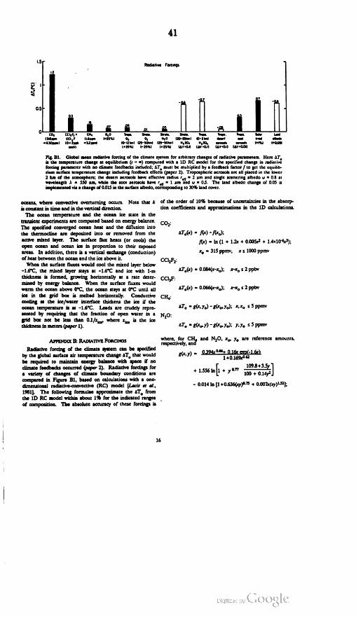
41

1.5Rodiative Forcings

12

을

0706

0.5

0.3

07

SaleCO , CC izle( 315ppm cci,

630ppm ) 10.2PPDwach )

сн .( 1.6 ppo

12pont

N ,0(* 25 % )

.09 OS.01

Tropo. Siroto Strato .O , Myo

(0-12 km ) (25-50m) 125-50 lum )(-25 % )

Streto .120-25 m )MASO

(AT.0.1)

Tropo10-2 )

M ,SO( AT + 0.1 )

Trope . Trope.desert toolosals coronas

(ATQI) (Ar.2011

( + Qos )

Fig. B1. Global mean radiative forcing of the climate system for arbitrary changes of radiative parameters. Here AT .

is the temperature change at equilibrium ( - ) computed with a ID RC model for the specified change in radiative

forcing parameter with no climate feedbacks included ; at, must be multiplied by a feedback factorf to get the equilib

rium surface temperature change including feedback effecis (paper 2). Tropospheric acrosols are all placed in the lower

2 km of the atmosphere; the desen acrosols have effective radius Ferie - 2 um andsingle scattering albedo w =0.8 at

wavelength 1 = 550 nm , while the soot aerosols have leres 1 um and w = 05. The land albedo change of 0.05 is

implemented via a change of 0.01S in the surface albedo, corresponding to 30 % land cover.

oceans, where convective overturning occurs . Note that k of the order of 10% because of uncertainties in the absorp

is constant in time and in the vertical direction . tion coefficients and approximations in the ID calculations.

The ocean temperature and the ocean ice state in the

transient experimentsare computed based onenergybalance. coz:The specified converged ocean heat and the diffusion into

the thermocline are deposited into or removed from the AT . (x ) = f (x ) -* );

active mixed layer. The surface flux heats (or cools) thef(x ) = In (1 + 1.2x + 0.0052 + 1.4x10-6 ? );

open ocean and ocean ice in proportion to their exposed

areas. In addition, there is a vertical exchange ( conduction) Xo = 315 ppmv, xs 1000 ppmv

of heat between the ocean and the ice above it . CCl2Fz:When the surface fluxes would cool the mixed layer below

-1.6 ° C , the mixed layer stays at -1.6 ° C and ice with 1-m AT . (x) = 0.084( x - x . ); x-* , s 2 ppbv

thickness is formed, growing horizontally at a rate deter- CC13F :

mined by energy balance. When the surface fluxes would

warm the ocean above 0 ° C , the ocean stays at 0 ° C until allAT .( x) = 0.066 (x -x .); x - x , s 2 ppbv

ice in the grid box is melted horizontally. Conductive CHA:

cooling at the ice /water interface thickens the ice if the

ocean temperature is at -1.6°C. Leads are crudely repre AT . - g (x, y ) -864o,yo); * , * , s 5 ppmy

sented by requiring that the fraction of open water in a NO:

grid box not be less than 0.1 / Zice, where zice is the ice

thickness in meters (paper 1). AT . -8(* o, Y) -864o,yo); y,yo s5 ppmv

APPENDIX B: RADIATIVE FORCINGS

Radiative forcing of the climate system can be specified

by the global surface air temperature change AT . that would

be required to maintain energy balance with space if no

climate feedbacks occurred (paper 2 ). Radiative forcings for

a variety of changes of climate boundary conditions are

compared in Figure B1, based on calculations with a one

dimensional radiative - convective (RC ) model (Lacis et al.,

1981). The following formulae approximate the at , from

the iD RC model within about 1 % for the indicated ranges

of composition. The absolute accuracy of these forcings is

where, for CH , and N2O , X, Yo are reference amounts,respectively, and

8(x, y) = 0.394 0.66+ 0.16r exp( -1.6x)

1 + 0.16 % -0.62

109.8 + 3.5y+ 1.556 In 1 + y 0.77

100+ 0.14y2

- 0.014 In ( 1 + 0.636 (xy )0.75 + 0.007x (xy) 1-52 ];

- 1.556 1n [1+

16

1

42

Specifically, in scenario A Co , increases as observed by

Keeling for the interval 1958-1981 (Keeling et al., 1982)

and subsequently with 1.5 % yol growth of the annual

H2SO , aerosols ( 20 km ): increment. CCLF ( F-11) and CCLF, ( F -12) emissions are

AT .(1 ) = -5.81; + (1 = 550 nm ) s 0.2from reported rates (Chemical Manufacturers Association

(CMA) 1982) and assume 3% yrd increased emission in the

H2SO , aerosols (0-2km ): future, with atmospheric lifetimes for the gases of 75 and

AT (1) = -6.51; 9 (1 = 550 nm ) s 0.2150 years, respectively. CH , based on estimates given by

Lacis et al. (1981), increases from 1.4 ppbv in 1958 at a rate

Solar irradiance: of 0.6 % yr until 1970, 1% yrıl in the 1970s and 1.5% yr -1

AT . ( -) = 0.67x ; * = AS. ( % ) s 1%thereafter. N20 increases according to the semiempirical

formula of Weiss ( 1981), the rate being 0.1% yr in 1958, 0.2 %

Land albedo: yrl in 1980, 0.4% yrs in 2000, and 0.9 % yrl in 2030 .

AT . ( t) = -0.12 %, x- A albedo of land area s 0.1 Potential effects of several other trace gases ( such as Oz,

stratospheric H2O, and chlorine and fluorine compounds

Trace gas scenarios. Trace gas trends beginning in 1958 other thanCCLF and CCLF ) are approximated by multi

(when accurate measurements of Co , began )wereestimated plying the CCLFand CCLF amountsby2.

from measurement data available in early 1983, when we In scenarioB the growth of the annual increment of Co ,

initiated our transient simulations. References to the is reduced from 1.5 % yrd today to 1% yol in 1990,

measurements are given by Shands and Hoffman (1987). 0.5 % yrd in 2000, and 0 in 2010; thus after 2010 the annual

Figure B2 summarizes the estimated decadal increments to increment in co , is constant, 1.9 ppmv yr'? The annual

global greenhouse forcing. The forcings shown by dotted growth of CCIF andCCLF , emissions is reduced from 3%

lines in Figure B2 are speculative; their effect was included yr today to 2 % yıl in 1990, 1% yrs in 2000 and 0 in

in scenario A but was excluded in scenarios B and C. The 2010. The methane annual growth rate decreases from 1.5 %

CH , forcing in the 1980s represents a 1.5 % yra growth yra today to 1.0 % in 1990 and 0.5 % yrd in 2000. NGO

rate; recent data ( Bolle et al., 1986, Blake and Rowland, increases are based on the formula of Weiss (1981), but

1987) suggest that a 1.1% yr growth rate probably is more the parameter specifying annual growth in anthropogenicrealistic . emission decreases from 3.5 % today to 2.5 % in 1990,

0.10

DECADAL INCREMENTS OF GREENHOUSE FORCING

0.08

-

03

St He

0.06

-

F11

ATO

(°C)

CF Mugo CO2F12

F110.04

-

CO2CO2 : 87 str .

F12

Meno

CFCS 15.6

0.02 )12.8

CO2 8.2 NO pomF12

NOpom CHA

03 St,Hopm

CHApom

-MOCHA

1850 - 1960 1960's 1970's 1980's

(per decade)

DECADES

Fig. B2. Estimated decadal additions to global mean greenhouse forcing of the climate system . The value of AT . is

defined in the caption of Figure Bl. Forcings shown by dotted lines are highly speculative.

17

43

0.04

0.03

0.02Optical

Depth

QOI

-0.01ISSO 1969 1970 1975 1979

Dote

1.5% in 2000, and 0.5 % in 2010. No increases are included with 2 times greater a in the northern region than in the

for other chlorofluorocarbons, Og, stratospheric H20, or any Southern region. Beginning 10 months after the eruption, 1

other greenhouse gases. decayed exponentially with a 12 -month time constant.

In scenario C the CO2 growth is the same as in scenarios

A and B through 1985;between 1985 and 2000 the annual

co , incrementis foxed at 1.5 ppmv yr *?; after 2000, CO2 Aerosol Optical Depth of Mouno Loo

ceases to increase, its abundance remaining fixed at 368

ppmv. CCIF and CCLF, abundances are the same as in

scenarios A and B until1990; thereafter, CCIF and CCLF2

emissions decrease linearly to zero in 2000. CH , abundance

is the same as in scenarios A and B until 1980; between

1980 and 1990 its growth rate is 1% yr !; between 1990 and

2000 its growth rate is 0.5 % yr ?; after 2000, CH, ceases to

increase, its abundance remaining fixed at 1916 ppbv. As in

scenario B , no increases occur for the other chlorofluoro

carbons, Og, stratospheric H20 , or any other greenhouse

gases.

Scratospheric aerosol scenarios. The radiative forcing dueWh

to stratospheric aerosols depends principally upon their

optical thickness at visible wavelengths, their opacity in the Fig. B3. Aerosol optical depth measured at Mauna Loa (light

thermal infrared region, and their global distribution. curve )after subtraction of the mean value for 1958–1962. The

Because of the small size of long-lived stratospheric heavy line istheoptical depthat Mauna Loa,obtained from the3Daerosols, their effect on planetary albedo generally exceeds tracermodel, as discussedin the text. The arrows mark the timestheir effect on infrared transmission (Hansen et al., 1980 ). of eruption ofAgung, Awu, Femandina and Fuego, respectively .

Thus the most important acrosol radiative parameter is the

optical thickness at visible wavelengths, 1. We base the The optical properties of the stratospheric aerosols beforeestimated , before El Chichón primarily on solar trans- 1982 are based on measurements of Agung aerosols. The

mission measurements at Mauna Loa (Mendonca, 1979), size distribution we used is that given by Toon and Pollack

together with calculations with a 3D tracer model (Russell ( 1976 ), which is based on measurements by Mossop ( 1964 ); itand Lemer, 1981). has mean effective radius and variance (Hansen and Travis,

The measured optical depth at Mauna Loa, after subtrac- 1974) of regs * 0.2 im and ved * 0.6. These aerosols are

tion of the mean 1958-1962 value, which is assumed to assumed to be spheres of sulfuric acid solution (75 % acid by

represent the local background value, is shown as the light weight) with refractive index given by Palmer and Williams

line in Figure B3. An arbitrary amount of tracer substance ( 1975). We used size data for the Ei Chichón aerosolswas introduced in the stratosphere of the tracer model at based on measurements of Hoffman and Rosen (1983). Their

the time and location of the volcanic eruptions of Agung May 1982 data had rett • 1.4 um , veme * 0.4, while their

( 1963 ), Awu ( 1966 ), Fernandina ( 1968) and Fuego (1974 ). October 1982 data had rete * 0.5 um , vere * 0.15. We

The computed amount of tracer at Mauna Loa was then interpolated linearly between these two size distributions for

multiplied by the scale factor required such that the the 6 month period April 1982 to October 1982, and

computed transmission equaled the mean measured trans- thereafter used the small-particle ( October 1982) size

mission at Mauna Loa in the two years following the distribution . These various size distributions yield the same

cruption; the modeled aerosol opacity is illustrated by the cooling at the Earth's surface as a function of 2 (1 - 550

heavier line in Figure B3. The tracer model thus defined nm ) within a few percent, as computed with the ID RC

the global distribution of aerosol optical depth for the model, but the large particles cause a greater stratospheric

period 1958–1979 . heating. For example, the May 1982 distribution yields a

The aerosol optical depths for El Chichón, based on early warming of 5 °C at 23 km , the Oaober 1982 distribution

reports (M. P. McCormick, privatecommunication ), later yields 2 °C, and the Mossop (1964) aerosols yield 1.5 ° C .published by McCormick et al., ( 1984 ), were specified as An extensive measurement campaign was mounted after

follows. For the first 6 months after the eruption, the the El Chichón eruption in 1982, which will allow a more

opacity was uniformly distributed between the equator and precise calculation of the geographical and altitute distri

30°N , increasing linearly from 1=0 at the time of eruption bution of the radiative forcing than for any previous

to q = 0.25 3 months after the eruption and remaining volcano. We are working with J. Pollack and P. McCormickconstant for the next 3 months. Subsequently, the opacity to make use of the fulldata now available for a compre

was uniform from 90 ° to 30 °N and from 30° N to 90 °S, but hensive study of the climate impact in that period.

18

44

However, the scenarios in our present simulations were Hansen, J., and S. Lebedeff,Global trends of measured surface air

defined in early 1983 when only sketchy data on the El temperature, J. Geophys. Res.92, 13,345-13,372, 1987.

Chichón acrosols were available, so the uncertainty in theHansen, J., and S. Lebedeff, Global surface air temperatures: update

through 1987,Geophys. Res. Len ., 15, 323–326, 1988.aerosol forcing after El Chichón in our present simulations Hansen , J. E, and D. Travis , Light scattering in planetary

is comparable to that in the prior years. atmospheres,Space Sci. Rev., 16 , 527-610, 1974.

Hansen, J. E., W. C. Wang, and A. A. Lacis, Mount Agung eruption

provides test of a global climatic perturbation, Science, 199,

1065-1068, 1978 .

Hansen, J. E., A A. Lacis, P. Lec, and W.C. Wang, Climatic effects

of atmospheric aerosols, Ann . N. Y. Acad. Sci., 338, 575-587,

Acknowledgements. We thank Jim Angell,Alan Robock and Steve 1980 .

Schneider for comments on the first draft of this paper, Patrice Hansen, J., E. Johnson, A. Lacis, S. Lebedeff, P. Lee, D. Rind, and

Palmer and Jeff Jonas for helping produce the color ligures, Jose G. Russell, Climate impact of increasing atmospheric carbon

Mendoza for drafting other figures, and Carolyn Paurowski for dioxide, Science, 213, 957-966, 1981.

desktop typesetting. This work has been supported by the NASA Hansen , J., G. Russell,D. Rind, P. Stone, A Lacis, S. Lebedeff,

Climate Program and EPA grant R812962-01-0 . R Ruedy and L. Travis, Efficient three -dimensional global

models for climate studies: models I and II, Mon. Weather Rev.,

111, 609-662, 1983

REFERENCESHansen, J., A. Lacis, D. Rind, G. Russell, P. Stone, 1. Fung,

R Ruedy, and J. Lemer, Climate sensitivity. Analysis of feedback

Alexander, R C., and R L Mobley, Monthly average sea-surface mechanisms, in Climate Processes and Climaie Sensitivity,

temperature and ice-pack limits on a 1* global grid , Rep. 4-1310 Geophys. Monogr. Sat., Vol. 29 , edited by J. E. Hansen and

ARPA,30pp., Rand Corp., Santa Monica, 1974. T. Takahashi,pp. 130–163,AGU, Washington, D.C., 1984 .

Angell, J. K., Annual and seasonal global temperature changes in Hansen, J., G. Russell, A. Lacis, I. Fung, D.Rind, and P. Stone,

the troposphere and low stratosphere, 1960–1985, Mon. Weather Climate response times:Dependenceon climate sensitivity andRav ., 114, 1922-1930, 1986 . ocean mixing, Science, 229, 857-859, 1985.

Barnett, T. P., Detection of changes in the global troposphere Hansen, J., 1. Fung, A. Lacis, S. Lebedeff, D. Rind, R Ruedy, andtemperaturefield induced by greenhouse gases, J. Geophys. Res., G. Russell, Predictions of near - term climate evolution : What can

91,6659-6667, 1986. we tell decision makers now ?, paper presented at First North

Bell, T. L , Optimal weighting of data to detect climate change: American Conference on Preparing forClimate Change, Climate

Application to the carbon dioxide problem , J. Geophys. Res., 87, Institute, Washington, Oct. 27–29, 1987.

11,161-11,170, 1982 . Hasselmann ,K , Stochastic climate models, I. Theory, Tellus, 28,Blake, D. and S. Rowland , Increasing global concentrations 473-485, 1976 .of tropospheric methane, paper presented at Symposium on Hoffman, D. J., and J. M. Rosen, Sulfuric acid droplet formationAtmospheric Methane. Am . Chem . Soc., Denver, Colo ., and growth in the stratosphere after the 1982 eruption of El

April 5-10, 1987. Chichón, Science, 222, 325-327, 1983.

Bolle, H. J., W. Sciler, and B. Bolin, Other greenhouse gasesand Keeling, C D., R. B. Bacastow, and T. P. Whorf, Measurements ofacrosols, in The Greenhouse Effeci, Climate Change, and Eco the concentration of carbon dioxide at Mauna Loa observatory,

systems, edited by B. Bolin , B. A. Doos, J. Jager and R A. Hawaii, in Carbon Dioxide Review : 1982, edited by W. C. Clark,

Warrick, pp. 157–203, John Wiley, New York, 1986. pp. 377–385,Oxford University Press, New York, 1982.

Broecker, W. S., D. M. Peteet, and D. Rind, Does the ocean - atmo Lacis, A., J. Hansen, P. Lee, T. Mitchelland S. Lebedeff, Green

sphere system have more than one stable mode of operation ?, house effectof trace gases, 1970–1980, Geophys. Res. Leu ., 8,

Nature, 315, 21-26 , 1985. 1035-1038 , 1981.

Bryan, K., F. G. Komro , and C Rooth, The ocean's transient Lamb, H. H., Volcanic dust in the atmosphere; With a chronology

response to global surface temperature anomalies, in Climate and assessment of its meteorological significance, Philos. Trans.

Processes and Climate Sensitiviry, Geophys. Monogr. Ser ., Vol. 29, R Soc. London, Sa. A., 266, 425-533, 1970.

edited by J. E Hansen and T. Takahashi, pp. 29–38, AGU, Lemon, E R (ed.), Co , and Planks: The Response of Plants to

Washington D.C., 1984 . Rising Levels of Atmospheric Carbon Dioxide, MAAS Sel. Symp.

Charlson, R J., J. E Lovelock, M. O. Andreae, and S. G. Warren, Vol. 84, Westview Press, Boulder, Colorado, 1983.

Oceanicphytoplankton,atmospheric sulphur, cloud albedoand Levitus,S., Climatological Atlas of the World Ocean , NOAA

climate, Nature,326, 655-661, 1987, Prof. Pap . 13, Natl. Oceanic and Atmos. Admin.,

Charney, J., Carbon dioxide and climate: A scientific assessment, Washington, D.C., 1982.

33 pp., National Academy Press, Washington, D.C., 1979. Loreaz ,E N., Climatic determinism , Meteorol. Monograph., 30,

Chemical Manufacturers Association , World production and release 1-3, 1968

of chlorofluorocarbons 11 and 12through 1981 , Calculations by Manabe, S., and K. Bryan, CO2-induced changein a coupledocean

EI. du Pont de Nemours and Company, Inc., Washington, D.C., atmosphere model anditspaleoclimatic implications, J. Geophys.

1982 Res., 90, 11,689–11,707, 1985.

Davis,M.B., Lags in vegetation response to climate change, Clim . Manabe, S., and R J. Stouffer, Sensitivity of a global climate

Change, in press, 1988. model to an increase of co , concentration in the atmosphere,

Dickinson, Ř E , The climate system and modeling of future J. Geophys. Res., 85, S529-5554, 1980.

climate, in The Greenhouse Effecs Climate Change, and Eco Manabe, S., and R.T. Wetherald, The effects of doubling thesystems, edited by B. Bolin , B. A. Doos, J. Jager, and RA co , concentration on theclimate of a general circulation model,

Warrick, pp . 206-270, John Wiley, New York, 1986 . J. donos. Sci., 32, 3–5, 1975.

Prohlich, C., Variability of the solar " constant on time scales of Manabe, S., and R T. Wetherald, Large-scale changes of soil

minutes to years , J. Geophys. Res., 92, 796-800, 1987. wetness induced by an increase in atmospheric carbon dioxide,

J. Aomos. Sci., 44 , 1211-1235, 1987.

19

45

McCormick, M. P., T. J. Swissler, W. H. Fuller, W. H. Hunt, and Toon, O. B., and J. B. Pollack, A global average model of

M. T. Osborn, Airbome and ground -based lidar measurements of atmospheric acrosols for radiative transfer calculations, J. Appl.

the ElChichón stratospheric aerosol from 90 ° N to 56 °S , Geofis. Mescorol., 15, 225-246, 1976 .

Inil , 23, 187-221, 1984 . Walsh, J., and C Johnson, An analysis of Arctic sea ice fluctua

Meams, L 0., R W. Katz and S. H. Schneider, Extreme high tions, J.Phys. Oceanogr., 9, 580-591, 1979 .

temperature events: changes in their probabilities with changes in Wang, W. C., G. Molnar, T. P. Mitchell, and P. H. Stone, Effects ofmean temperature, J. Clim .Appl. Mereorol., 23, 1601-1613, 1984. dynamical heat fluxes on model climate sensitivity, J. Geophys.

Mendonca,B. G. (Ed.), Geophysical Monitoring for Climate Res., 89, 4699-4711, 1984 .

Change, No. 7, Summary Report 1978, 131 pp., NOAA Envir. Res. Wang, W. C., Y. L Yung, A. A. Lacis, T. Mo and J. E. Hansen,

Lab., Boulder, Colorado, 1979. Greenhouse effects dueto man -made perturbations of trace gases,Miller, J. R , G. L. Russell and L C. Tsang, Annual oceanic heat Science, 194,685-690, 1976 .

transports computed from an atmospheric model, Dyn. Aimos. Washington, W. M.,and G. A. Mechi, Seasonal cycle experiment on

Oceans, 7, 95-109, 1983 . the climate sensitivity due to adoubling of co, with an atmos

Mitchell, J. M., A preliminary evaluation of atmospheric pollution as pheric general circulation model coupledto a simple mixed -layer

aause of global temperature fluctuation of the pastcentury, in ocean model,J. Geophys. Res., 89, 4475-9503, 1984.

Global Effects of Environmenial Pollution, edited by S. F. Singer, Weiss, R P.,The temporal and spatial distribution of tropospheric

pp. 139–155, Springer - Verlag, New York, 1970. nitrous oxide, J. Geophys. Res ., 86, 7185-7195, 1981.

Mossop, S. Com Volcanic dust collected at an altitude of 20 km , Willson, R C., and H. S. Hudson, Solar luminosity variations in

Nature, 203, 824-827, 1964 . solar cycle 21, Nature, 332, 810–812, 1988.

National Academy of Sciences, Understanding Climatic Change, Willson ,R C , H. S. Hudson, C. Frohlich, and R.W. Brusa, Long

239 pp ., Washington,D.C., 1975.term downward trend in total solar irradiance , Science, 234,

National Oceanographic and Atmospheric Administration, User's 1114-1117, 1986.

Guide to NODC Data Services, Environmental Data Service, Wilson, C. A., and J. F. B. Mitchell, A 2XCO , climate sensitivity

Washington, D.C., 1974. experiment with a global climate model including a simple ocean,

Palmer, K F., and D. Williams, Optical constants of sulfuric acid , final report CEC contract CL- 114 UK (H), British Meteorol.

Applications to the clouds of Venus ?, Appl. Opt., 14, 208-219, Office , Bracknell, U.K., 1987.

1975.

Peixoto, J. P., and A. H. Oort, Physics of climate. Rev. Mod. Phys.,S6 , 365-429, 1984 . I. Fung, J. Hansen, A. Lacis, S. Lebedeff, D. Rind, R Ruedy and

Pollack, J. B., O. B. Toon, C. Sagan, A. Summers, B. Baldwin and G. Russell, NASA Goddard Space Flight Center, Goddard Institute

W.Van Camp, Volcanic explosions andclimatic change: A theo for Space Studies, 2880 Broadway, NewYork, NY 10025 .

retical assessment, d. Geophys. Res.,81, 1071-1083, 1976 . P. Stone, Center for Meteorology and Physical Oceanography,

Ramanathan, V., R J. Cicerone, H. B. Singh, and J. T. Kichl, Trace Massachusetts Institute of Technology, Cambridge, Massachusetts

gas trends and their potential role in climate change, J. Geophys. 02139.

Res., 90,5547-5566, 1985.

Rind, D., R Suozzo, N. K. Balachandran, A. Lacis, and G. Russell,

The GISS global climate /middle atmosphere model, Part I Model

structure and climatology, J. Aomos. Sci., 45, 329-370, 1988.

Roberts, L., Coral bleaching threatens Atlantic reefs, Science, 238,

1228-1229, 1987.

Robinson, M., and R Bauer, Oceanographic Monthly Summary 1,

No. 2, pp . 2–3, NOAA Natl. Weather Serv ., W322, Washington,

D.C., 1981.

Robock, A., Internally and externally caused climate change,

J. Atmos. Sci., 35, 1111-1122, 1978 .

Robock, An, A latitudinally dependent volcanic dust veil index, and

its effect on climate simulations, J. Volcanol. Geotherm . Res., II ,67-80, 1981.

Russell, G. L , and J. A. Lemer, A new finite-differencing

scheme for the tracer transport equation , J. Appl. Meteorol., 20,1483-1498, 1981.

Russell, G. L., J. R Miller and LC Tsang, Seasonal oceanic heat

transports computedfrom an atmospheric model, Dynam . Atmos.Oceans, 9, 253–271, 1985.

Schneider, S. H., and S. L Thompson, Atmospheric co , and

climate: importance of the transient response, J. Geophys.Res.,

86, 3135–3147, 1981.

Schneider, S. H., and C Mass, Volcanic dust, sunspots, and

temperature trends, Science, 190, 741-746, 1975.

Shands, W. E , and J. S. Hoffman, (Ed .), The Greenhouse Effeci,

Climate Change, andU.S.Foresis, 304 pp, Conservation Founda

tion, Washington, D.C., 1987.

Smagorinsky, J., Carbon dioxide and climate : A second assessment.

239 pp, National Academy Press, Washington, D.C., 1982 .

Somerville, R C J., and L A Remer, Cloud optical thickness

feedbacks in the co , climate problem , J. Geophys. Res ., 89,9668-9672 , 1984.

20

46

Plate 1. Interannual variability (standard deviation ) of temperature in the 100 year control run ( left side) and as

estimated from observations ( right side). (a ), (b ), (c ) and ( ) show the interannual variability of surface air tempera

ture, and ( e )and( ) show the interannual variability of the longitude-integrated upper air temperature. (6) and (d) are

based on 1951–1980 observations at meteorological stations analyzed by Hansen and Lebedeff ( 1987 ). V is based on

1958–1985 radiosonde data analyzed byAngell (1986 ). Regions without data are black.

Plate 2. Left side: decadal mean temperature change obtained for scenario B, relative to the control run , for the

decades 1980s, 1990s and 2010s. Right side: ratio of the computed temperature change to the interannual variability of

the annual mean temperature in the 100 year control run (Plate la).

Plate 3. Left side: decadal mean temperature change for scenario B as a function of latitude and season , for the

decades 1980s, 1990s and 2010s. Right side: ratio of the computed temperature change to the interannual variability of

the monthly mean temperature in the 100 year control run ( Plate 1c)

Plate 4. Left side: decadal mean temperature change for scenario B as a function of pressure and latitude, for the

decades 1980s, 1990s and 2010. Right side: ratio of the computed temperature change to the interannual variability of

the annual mean temperature in the 100 year control run (Plate le).

Plate S. Simulated June- July-August (left side) and December-January - February temperature anomalies in the 1990s,

compared to the 100 year control run with 1958 atmospheric composition .

Plate 6. Simulated July surface air temperature anomalies for six individual years of scenario B, compared to the 100

year control run with 1958 atmospheric composition.

1

47

90 ALU SARUN OBSERVED

300 30

20 18 -720 60 80

25 50 75

c ) NON ALYT DYEAR RUN OBSERVED

300V

50

SONO

AL

MOSS

30 50

48

-3

OBD

O21

.09

09

021

OB1

180

021

09

-60

OZI

08106

08

0

30

09

LIR

06

0102

06

-60

-300

30

-109

90

$0661

5,066

06

09

-30

030

TE

60

7

1980's

/19

QIHVNOS

1980's

90

SCENARIO

BAT

1°c)

49SCENARIO

&T(°C)90

1980's

SCENARIO

BATI

1980

'

60 d

LATITUDE

0 -30

09 -

06

1990's

1990's

90

LATITUDE

-30

-60

-90

2010's

2010

90

30

LATITUDE

0

30

-60

06-

JFM AM JJ ASO ND

MONTH

MAM

WV

A SON D

MONTH

-3-2

T

23434

567

1

50

SCENARIO

BAT

(°c)1980's

SCENARIO

BAT

/1980's

200

400

( AN ) 380ssd

600

800

1000

1990's

1990's

o

200

400

PRESSURE(MB)

600

800

1000

2010's

2010's

200

400

PRESSURE(MB)

600

800

1000

60

30

-60

-90

06

o-30

LATITUDE

09

30

-60

-90

LATITUDE

-1.5-1

.-500.5

1

1.5

2.5

-6-4

-2

02468

51

SCENARIO

90

AAT

(9)JUN

-AUG

,1990

$SCENARIO

Aat

(°C)DEC

-FEB

,1990

60 30 o

bo

-30

-60

-90

SCENARIO

890

SCENARIO

8

7

601

30

0 -30

-60

-90

SCENARIO

C90

SCENARIO

C

?

601

30

0 1-30

-60

-90-180

-120

60

60

120

180

-180

-120

-60

o

60

120

180

-22

!

1

52

SCENARIO

.B

MEAN

AT

:+0.2

°CJULY

1986

MEAN

AT

+0.6

°CJULY

2000

60 0

-30

-60

-

-90

MEAN

01

:+0.3

° CJULY

1987

MEAN

OT

:+10

°CJULY

2015

06

60

30

0

-30

-60

-90

MEAN

AT

:+0.5

°C90

JULY

1990

MEAN

AT

:+1.5

°CJULY

2029

7

09

30 o

-30 -180

-120

09

60

120

180

-180

-120

-60

09

120

081

Arlºc

)

-3

2

53

Mr. SHARP. Thank you very much, Dr. Hansen . Dr. MacCracken .

STATEMENT OF MICHAEL C. MacCRACKEN

Mr. MacCRACKEN. Thank you, Mr. Chairman . I've been invited

to come and provide some perspective on limitations and uncertain

ties in our understanding.This is not an easy topic becauseitgets

into discussing details and nuances of how things are done. I think

it's a very important one and it raises some very important issues

to be considering.

First, I'd like to say that I agree with the previous speakers and I

think there's a broad scientific consensus that the greenhouse

effect is real. It's not the only factor that's probably affecting the

climate, but it's probably the most important one. We are changing

atmospheric composition. This is going to cause the temperature to

rise, not by perhaps tenths ofa degree, but by degrees. It's going to

cause sea levels to rise and it's going to cause shifting of precipita

tion .

There are many things we don't know about this and there are

many reasons that uncertainties arise about how much the emis

sions will bein the future; how the atmospheric composition and

chemistry will change; how climate will change; how the environ

ment will respond and I'm just going to focus on the climate as

pects of that here.

The questions that come up are by how much the climate will

change ; where it will occur and when it will happen. I think the

uncertainty, the level of uncertainty that exists in this, is of the

order of a factor of 2, on many kinds of questions — how much the

warming might be in a hundred years in the midwestern United

States; or how much sea level might rise over the next hundred

years.

They are not factors of 10 uncertainty; they're factors of 2 uncer

tainty. But these can stillbe important andraise interesting policy

kinds of questions. First, I should say that this is a very, very diffi

cult question to work on. It's a little bit like predicting what's

goingto — the details of what would happen if you have a cigarette

with smoke rising and you have all the little eddies. The little

eddies that are occurring and waves and things that are happen

ing, are the weather that one would be experiencing; predicting

that into the future, is very, very hard . It's something that we can

try to do and we can try and figure out how wide thesmoke plume

might be and what the frequency of these eddies might be, to give

us a sense ofwhat's happening.

Basically , Jim Hansen has talked about his research . There are

four groups in the United States and several others abroad that are

studying this problem . The four U.S. groups in addition to the

group at the Goddard, are at the Geophysical Fluid Dynamics Lab

oratory atPrinceton, at the National Center for Atmospheric Re

search in Boulder, and at Oregon State University.

Each of these groups has been working for more than a decade,

with what resources they have, to do thebest possible job that they

can. These models, still, however, have quite a number of shortcom

ings that are important to consider. What we have been doing at

Livermore on behalf of the Department of Energy, is looking at

.PUB

]ENERGY POLICY IMPLICATIONS OF GLOBAL

WARMING

2/3 UNIVERSITY OF CALIFORNIA

RIVERSIDE1-229

UNIVERSITY OF CA. RIVERSIDE LIBRARY

MAY 1 5 1989

3 1210 01570 1905

LIBRARY

GOVERNMENT PUBLICATIONS DEPT.

U.S. DEPOSITORY

HEARINGS

BEFORE THE

SUBCOMMITTEE ON

ENERGY AND POWER

OF THE

COMMITTEE ON

ENERGY AND COMMERCE

HOUSE OF REPRESENTATIVES

ONE HUNDREDTH CONGRESS

SECOND SESSION

JULY 7 AND SEPTEMBER 22, 1988

Serial No. 100-229

Printed for the use of the Committee on Energy and Commerce

U.S. GOVERNMENT PRINTING OFFICE

WASHINGTON : 1989961505

For sale by the Superintendent of Documents, Congressional Sales Office

U.S. Government Printing Office, Washington , DC 20402

toe COMMITTEE ON ENERGY AND COMMERCE

PHILIPRWA OD12.California »

1

j

JOHN D. DINGELL, Michigan, Chairman

JAMES H. SCHEUER , New York NORMAN F. LENT, New York

EDWARD R. MADIGAN , Illinois

CARLOS J. MOORHEAD, California

JAMESJ,FLORIO , New Jersey . ** MATTHEW J. RINALDO , New Jersey

EDWARD J. MARKEY, Massachusetts WILLIAM E. DANNEMEYER , California

THOMAS A. LUKEN , Ohio BOB WHITTAKER , Kansas

DOUG WALGREN , Pennsylvania THOMAS J. TAUKE, Iowa

AL SWIFT, Washington DON RITTER, Pennsylvania

MICKEY LELAND , Texas DAN COATS, Indiana

CARDISS COLLINS, Illinois THOMAS J. BLILEY, JR., Virginia

MIKE SYNAR , Oklahoma JACK FIELDS , Texas

W.J. " BILLY” TAUZIN , Louisiana MICHAEL G. OXLEY, Ohio

RON WYDEN , Oregon HOWARD C. NIELSON , Utah

RALPH M. HALL , Texas MICHAEL BILIRAKIS , Florida

DENNIS E. ECKART, Ohio DAN SCHAEFER , Colorado

WAYNE DOWDY, Mississippi JOE BARTON , Texas

BILL RICHARDSON , New Mexico SONNY CALLAHAN , Alabama

JIM SLATTERY, Kansas

GERRY SIKORSKI, Minnesota

JOHN BRYANT, Texas

JIM BATES, California

RICK BOUCHER , Virginia

JIM COOPER, Tennessee

TERRY L. BRUCE, Illinois

WM . MICHAEL KITZMILLER , Staff Director

MARGARET A. DURBIN , Minority Chief Counsel/Staff Director

SUBCOMMITTEE ON ENERGY AND POWER

PHILIP R. SHARP , Indiana , Chairman

DOUG WALGREN , Pennsylvania CARLOS J. MOORHEAD , California

AL SWIFT, Washington WILLIAM E. DANNEMEYER , California

MIKE SYNAR , Oklahoma JACK FIELDS, Texas

W.J. " BILLY" TAUZIN , Louisiana MICHAEL G. OXLEY, Ohio

BILL RICHARDSON , New Mexico MICHAEL BILIRAKIS , Florida

JOHN BRYANT, Texas DAN SCHAEFER, Colorado

TERRY L. BRUCE, Illinois JOE BARTON , Texas

EDWARD J. MARKEY, Massachusetts SONNY CALLAHAN , Alabama

MICKEY LELAND , Texas NORMAN F. LENT, New York

RON WYDEN , Oregon ( Ex Officio )

RALPH M. HALL, Texas

WAYNE DOWDY, Mississippi

JOHN D. DINGELL, Michigan

(Ex Officio )

JOHN A. Riggs, Staff Director

JUDI GREENWALD, Counsel

TERESA A. GORMAN , Minority Staff Associate

( II )

CONTENTS

Page

1

83

4

Hearings held on:

July 7, 1988 ...

September 22, 1988 ..........

Statement of:

Firor, John W., Director, Advance Study Program , National Center for

Atmospheric Research ...........

Fisher, Linda, Assistant Administrator for Policy Planning, and Evalua

tion , Environmental Protection Agency .....

Fitzpatrick , Donna R., Undersecretary, Department of Energy

Gibbons, John H., Director, Office of Technology Assessment...

Hansen, James E. , Chief, NASA Goddard Institute for Space Studies ..........

MacCracken , Michael C. , Division Leader, Atmospheric and Geophysical

Sciences Division , Lawrence Livermore National Laboratory

Mintzer,Irving, senior associate, Energy, Climate, and Air Pollution Pro

gram , WorldResources Institute ...

Material submitted for the record by:

American Forestry Association , statement ........

Energy Department, " Public Papers of the Presidents"

165

85

191

15

53

108

262

217

( III )

..

This is a reproduction of a library book that was digitized by Google as part of an ongoing effort to preserve the information in books and make it universally accessible.

https://books.google.com