
Working time: Theory and policy implications
250
This is page i Printer: Opaque this WORKING TIME. Theory and Policy Implications François CONTENSOU Radu VRANCEANU January 23, 2000
Transcript of Working time: Theory and policy implications

This is page iPrinter: Opaque this
WORKING TIME.Theory and Policy Implications
François CONTENSOU Radu VRANCEANU
January 23, 2000
vranceanu
Text Box
Please cite as: François Contensou and Radu Vranceanu, Working Time. Theory and Policy Implications, Edward Elgar, Cheltenham, UK, 2000. ISBN 1-85898-996-5
vranceanu
Text Box
Pre-print version

ii
ABSTRACT This is a blank page. page ii

iii
Pages iii

iv
Page iv.

This is page vPrinter: Opaque this
Contents
Foreword xv
1 Brief history of working time theory 11.1 The Mercantilists and the scarcity of labor . . . . . . . . . . 11.2 The Classics and Marx . . . . . . . . . . . . . . . . . . . . . 3
1.2.1 Smith and Marx on working time . . . . . . . . . . . 31.2.2 Reported facts and their interpretation in Marx’s ap-
proach . . . . . . . . . . . . . . . . . . . . . . . . . . 41.2.3 Other facts and alternative interpretations . . . . . . 51.2.4 The exploitation paradox . . . . . . . . . . . . . . . 6
1.3 Early neoclassical views . . . . . . . . . . . . . . . . . . . . 71.3.1 Léon Walras and the consistency of private decen-
tralized economies . . . . . . . . . . . . . . . . . . . 71.3.2 Jevons’ utility and disutility analysis . . . . . . . . . 81.3.3 A controversy about the short run supply of labor . 10
1.4 Conclusion . . . . . . . . . . . . . . . . . . . . . . . . . . . 12
2 Basic facts 152.1 Trends in working hours . . . . . . . . . . . . . . . . . . . . 162.2 Hours of work: structure . . . . . . . . . . . . . . . . . . . . 222.3 Do people think they work too much? . . . . . . . . . . . . 232.4 Conclusion . . . . . . . . . . . . . . . . . . . . . . . . . . . 27
3 Working time policy: an overview 29

vi Contents
3.1 Why regulate working time? . . . . . . . . . . . . . . . . . . 293.2 Work-sharing methods in international comparison . . . . . 313.3 Working time reduction: three country cases . . . . . . . . . 33
3.3.1 France: reducing working time by law . . . . . . . . 333.3.2 Germany: negotiated working time reduction . . . . 363.3.3 Japan: another way of negotiating . . . . . . . . . . 37
3.4 Working time: regulation vs. flexibility . . . . . . . . . . . . 393.5 Conclusion . . . . . . . . . . . . . . . . . . . . . . . . . . . 40
4 The standard neoclassical view of the labor market 434.1 Introductory considerations . . . . . . . . . . . . . . . . . . 43
4.1.1 The demand for labor services: the perfect homogene-ity assumption . . . . . . . . . . . . . . . . . . . . . 43
4.1.2 Equilibrium and rationing . . . . . . . . . . . . . . . 454.2 The neoclassical hours supply . . . . . . . . . . . . . . . . . 47
4.2.1 Main assumptions about workers’ constraints and pref-erences . . . . . . . . . . . . . . . . . . . . . . . . . 47
4.2.2 Optimal working time: the individual supply of hours 504.2.3 The compensated working time supply . . . . . . . . 524.2.4 The response of the individual labor supply to the
wage rate . . . . . . . . . . . . . . . . . . . . . . . . 534.2.5 Empirical estimates of labor supply functions . . . . 554.2.6 Surplus from work . . . . . . . . . . . . . . . . . . . 56
4.3 Comments on the elementary neoclassical model of hourssupply . . . . . . . . . . . . . . . . . . . . . . . . . . . . . . 584.3.1 The composite good: a caveat about relative prices . 584.3.2 Labor supply, wages and competing home production 614.3.3 Reservation wage and lump-sum cost of working: a
quantum . . . . . . . . . . . . . . . . . . . . . . . . . 634.4 Conclusion . . . . . . . . . . . . . . . . . . . . . . . . . . . 654.5 Appendix: Examples of theoretical utility functions . . . . . 66
5 Working time, production and cost functions 695.1 Contemporary demand side contributions to working time
analysis . . . . . . . . . . . . . . . . . . . . . . . . . . . . . 695.1.1 The critique of the elementary neoclassical approach 695.1.2 Basic Generalized Production Functions . . . . . . . 725.1.3 Empirical estimates of constant output elasticity Gen-
eralized Production Functions . . . . . . . . . . . . . 765.2 A formal representation of the production decision . . . . . 77
5.2.1 Describing production and cost structures . . . . . . 775.2.2 Conventional production and cost functions . . . . . 785.2.3 Characterizing technologies and cost structures . . . 795.2.4 More definitions . . . . . . . . . . . . . . . . . . . . 805.2.5 Working with equipment . . . . . . . . . . . . . . . . 83

Contents vii
5.3 Production and cost functions . . . . . . . . . . . . . . . . . 845.3.1 Individual contribution functions . . . . . . . . . . . 845.3.2 Generalizing the representation of labor cost structure 84
5.4 Output density functions and cost density functions . . . . 855.4.1 The general form . . . . . . . . . . . . . . . . . . . . 855.4.2 Time profile of output density . . . . . . . . . . . . . 855.4.3 The Hicksian “optimal” day . . . . . . . . . . . . . . 865.4.4 Individual profile of output density . . . . . . . . . . 865.4.5 A simple optimal working schedule . . . . . . . . . . 87
5.5 The two dimensional demand for labor in the general case . 885.5.1 The cost minimization problem . . . . . . . . . . . . 885.5.2 Profit maximization . . . . . . . . . . . . . . . . . . 905.5.3 Profit maximization and the total demand for hours 91
5.6 The two dimensional demand for labor with a specific g.p.f. 915.6.1 From a simple o.d.f. to the specific g.p.f. . . . . . 915.6.2 Profit maximization and the demand for workers and
hours . . . . . . . . . . . . . . . . . . . . . . . . . . 925.6.3 Comparative statics of profit maximization: the im-
pact of varying wages . . . . . . . . . . . . . . . . . 945.6.4 On the impossibility of a decentralized equilibrium
in the labor market with a constant wage rate . . . . 955.7 Conclusion . . . . . . . . . . . . . . . . . . . . . . . . . . . 96
6 Working time in a cost minimization problem 996.1 Neoclassical production function with fixed costs of labor . 1006.2 Consequences of supply determined working time . . . . . . 1056.3 A more general approach: labor effectiveness . . . . . . . . . 106
6.3.1 The cost minimization problem . . . . . . . . . . . . 1066.3.2 Second order conditions . . . . . . . . . . . . . . . . 1076.3.3 Graphic solution . . . . . . . . . . . . . . . . . . . . 1086.3.4 An exercise of comparative statics . . . . . . . . . . 108
6.4 Cost minimization with factor substitution . . . . . . . . . 1106.4.1 The case with unconstrained working hours . . . . . 1106.4.2 The impact of a mandatory reduction in working hours111
6.5 Conclusion . . . . . . . . . . . . . . . . . . . . . . . . . . . 113
7 Cost minimization, heterogeneous workers and asymmetricinformation 1157.1 The decision problem of the firm . . . . . . . . . . . . . . . 116
7.1.1 Main assumptions and constraints . . . . . . . . . . 1167.1.2 Kuhn and Tucker conditions . . . . . . . . . . . . . 118
7.2 Optimal contracts and working time . . . . . . . . . . . . . 1197.2.1 The discriminating case . . . . . . . . . . . . . . . . 1197.2.2 Non-discriminating contracts . . . . . . . . . . . . . 120

viii Contents
7.2.3 The case of non-binding incentive compatibility con-straints . . . . . . . . . . . . . . . . . . . . . . . . . 123
7.3 Legal interference on working time . . . . . . . . . . . . . . 1267.4 Conclusion . . . . . . . . . . . . . . . . . . . . . . . . . . . 127
8 Premium pay for overtime 1298.1 Institutional schemes and possible supply response . . . . . 1298.2 Premium pay for overtime in a cost minimization set-up . . 1338.3 Comparative statics on hours . . . . . . . . . . . . . . . . . 1358.4 Conclusion . . . . . . . . . . . . . . . . . . . . . . . . . . . 136
9 Working time in a profit maximization framework 1399.1 Introduction . . . . . . . . . . . . . . . . . . . . . . . . . . . 1399.2 Main assumptions . . . . . . . . . . . . . . . . . . . . . . . 141
9.2.1 The workers’ consent to work . . . . . . . . . . . . . 1419.2.2 Generalized technology . . . . . . . . . . . . . . . . 143
9.3 The optimal contract: wages and hours . . . . . . . . . . . . 1449.3.1 Profit maximizing under the workers’ utility constraint1449.3.2 The special case of perfect man-hours substitution . 1479.3.3 The full-employment utility level . . . . . . . . . . . 148
9.4 Effect of a mandatory reduction of working time . . . . . . 1499.4.1 Sensitivity of employment to small variations of the
constraint . . . . . . . . . . . . . . . . . . . . . . . . 1509.4.2 Employment as a function of the working time con-
straint . . . . . . . . . . . . . . . . . . . . . . . . . . 1509.4.3 A simple simulation . . . . . . . . . . . . . . . . . . 151
9.5 Working time reduction under predetermined unemploymentbenefits . . . . . . . . . . . . . . . . . . . . . . . . . . . . . 152
9.6 Conclusion . . . . . . . . . . . . . . . . . . . . . . . . . . . 1549.7 Appendix I: Second order conditions . . . . . . . . . . . . . 1559.8 Appendix II: Comparative statics of fixed costs . . . . . . . 156
10 Working time in a trade union model 15710.1 Trade unions and hours negotiation . . . . . . . . . . . . . . 15710.2 Main assumptions . . . . . . . . . . . . . . . . . . . . . . . 160
10.2.1 The productive sector and the profit function . . . . 16010.2.2 The union’s objective function . . . . . . . . . . . . 161
10.3 Wage rate and working time are simultaneously negotiated 16210.4 Introducing a binding working time constraint . . . . . . . . 166
10.4.1 Analytical considerations . . . . . . . . . . . . . . . 16610.4.2 A numerical simulation . . . . . . . . . . . . . . . . 168
10.5 Conclusion . . . . . . . . . . . . . . . . . . . . . . . . . . . 16910.6 Appendix: Main elasticities and their relationships . . . . . 170

Contents ix
11 Complementary labor services and working time regula-tion 17311.1 Introduction . . . . . . . . . . . . . . . . . . . . . . . . . . . 17311.2 Main assumptions . . . . . . . . . . . . . . . . . . . . . . . 175
11.2.1 The production function and the structure of laborservices . . . . . . . . . . . . . . . . . . . . . . . . . 175
11.2.2 Worker compensating wage . . . . . . . . . . . . . . 17611.3 The unconstrained hours decision of the firm . . . . . . . . 176
11.3.1 The cost minimization problem . . . . . . . . . . . . 17711.3.2 Optimal employment . . . . . . . . . . . . . . . . . . 178
11.4 Employment under the hours constraint . . . . . . . . . . . 17911.4.1 The analytical approach . . . . . . . . . . . . . . . . 17911.4.2 A numerical example . . . . . . . . . . . . . . . . . . 179
11.5 Conclusion . . . . . . . . . . . . . . . . . . . . . . . . . . . 181
12 Working time reduction in a vertically integrated two-sectormodel 18312.1 Introduction . . . . . . . . . . . . . . . . . . . . . . . . . . . 18312.2 Explaining working time: a simple model of the labor contract185
12.2.1 The compensating wage function . . . . . . . . . . . 18512.2.2 The optimal contract . . . . . . . . . . . . . . . . . . 186
12.3 The vertical structure of the economy . . . . . . . . . . . . 18712.3.1 Sector 1: Production of the productive service. . . . 18712.3.2 Sector 2: Production of the consumption commodity 188
12.4 Equilibrium and comparative statics . . . . . . . . . . . . . 18812.4.1 A graphic introduction . . . . . . . . . . . . . . . . . 18812.4.2 The analytical approach . . . . . . . . . . . . . . . . 190
12.5 Special cases of fixed proportions . . . . . . . . . . . . . . . 19212.5.1 Fixed proportion of labor . . . . . . . . . . . . . . . 19212.5.2 Fixed proportion of output: the trucking case . . . . 193
12.6 Conclusion . . . . . . . . . . . . . . . . . . . . . . . . . . . 194
13 Working hours and unemployment in a matching model 19713.1 Introduction . . . . . . . . . . . . . . . . . . . . . . . . . . . 19713.2 Main assumptions . . . . . . . . . . . . . . . . . . . . . . . 199
13.2.1 The firm and its technology . . . . . . . . . . . . . . 19913.2.2 Workers’ consent to work and the labor contract . . 19913.2.3 The matching function . . . . . . . . . . . . . . . . . 201
13.3 The free profit maximization . . . . . . . . . . . . . . . . . 20213.3.1 Profit function and the optimal decision . . . . . . . 20213.3.2 Three basic equations . . . . . . . . . . . . . . . . . 20313.3.3 Equilibrium unemployment and hours of work . . . . 204
13.4 The policy of working time reduction . . . . . . . . . . . . . 20513.4.1 The steady state solutions . . . . . . . . . . . . . . . 20513.4.2 The adjustment dynamics . . . . . . . . . . . . . . . 206

x Contents
13.5 Conclusion . . . . . . . . . . . . . . . . . . . . . . . . . . . 208
14 Deregulation of overtime premium and employment dy-namics 20914.1 Introductory concepts: overtime and flexibility . . . . . . . 20914.2 Main assumptions . . . . . . . . . . . . . . . . . . . . . . . 21114.3 The cost minimization problem . . . . . . . . . . . . . . . . 212
14.3.1 Euler necessary conditions . . . . . . . . . . . . . . . 21214.3.2 First regime: the case with positive labor hoarding . 21314.3.3 Second regime: the production constraint is binding 213
14.4 A simplified dynamic submodel . . . . . . . . . . . . . . . . 21414.5 The labor cost functions and existence of labor hoarding
intervals . . . . . . . . . . . . . . . . . . . . . . . . . . . . . 21614.6 The case of a periodic activity constraint . . . . . . . . . . 21714.7 Conclusion . . . . . . . . . . . . . . . . . . . . . . . . . . . 21814.8 Appendix: Participation constraint . . . . . . . . . . . . . . 219
References 221
Index 230
Index 231

This is page xiPrinter: Opaque this
List of Figures
1.1 Optimal working time . . . . . . . . . . . . . . . . . . . . . 91.2 Demand for income and total hours supply . . . . . . . . . 12
4.1 Equilibrium wage . . . . . . . . . . . . . . . . . . . . . . . . 474.2 Network of indifference curves . . . . . . . . . . . . . . . . . 494.3 Hours supply . . . . . . . . . . . . . . . . . . . . . . . . . . 514.4 The reservation wage . . . . . . . . . . . . . . . . . . . . . . 524.5 Income and substitution effects . . . . . . . . . . . . . . . . 554.6 Surplus from work . . . . . . . . . . . . . . . . . . . . . . . 574.7 Compensation of a wage rate decrease . . . . . . . . . . . . 584.8 Optimal working time: at home and on-the-job . . . . . . . 624.9 Reservation wage with “commuting” costs . . . . . . . . . . 644.10 Involuntary unemployment . . . . . . . . . . . . . . . . . . 65
5.1 Standard effectiveness function . . . . . . . . . . . . . . . . 755.2 A special O.D.F. . . . . . . . . . . . . . . . . . . . . . . . . 925.3 Profit function . . . . . . . . . . . . . . . . . . . . . . . . . 935.4 Isoprofit network for predetermined wage . . . . . . . . . . 945.5 Optimal staff and working time under wage variation . . . . 955.6 Internal vs. external equilibrium . . . . . . . . . . . . . . . 96
6.1 Optimal working time . . . . . . . . . . . . . . . . . . . . . 1016.2 Cost minimizing contract under utility constraint . . . . . . 1026.3 Optimal contract: firm and worker point of view . . . . . . 103

xii Contents
6.4 Constrained working time . . . . . . . . . . . . . . . . . . . 1046.5 Optimal contract under hours supply constraint . . . . . . . 1066.6 Optimal working time: overwork . . . . . . . . . . . . . . . 1096.7 Optimal working time: insider underemployment . . . . . . 110
7.1 Optimal contracts: discrimination case . . . . . . . . . . . . 1217.2 Optimal contracts: non-discrimination case . . . . . . . . . 1247.3 Non-binding incentive constraints . . . . . . . . . . . . . . . 1257.4 Hours constraint and the optimal duration . . . . . . . . . . 127
8.1 Premium wage for overtime and the hours supply . . . . . . 1328.2 Cost minimizing hours . . . . . . . . . . . . . . . . . . . . . 1348.3 Impact of reducing statutory hours . . . . . . . . . . . . . . 136
9.1 Compensating wage function and workers’ rationing . . . . 1439.2 Labor contract setting: the general case . . . . . . . . . . . 1469.3 The case of perfect man-hours substitution . . . . . . . . . 1479.4 Flexible utility level and outside equilibrium . . . . . . . . . 1499.5 Working time constraints and the employment path . . . . 152
10.1 Equilibrium working time and workers’ compensation . . . 16510.2 Impact of the hours constraint on employment and other
variables . . . . . . . . . . . . . . . . . . . . . . . . . . . . . 169
11.1 Demand for less qualified workers . . . . . . . . . . . . . . . 18011.2 Demand for highly qualified workers . . . . . . . . . . . . . 18011.3 Total demand for workers . . . . . . . . . . . . . . . . . . . 181
12.1 Vertical structure of the economy . . . . . . . . . . . . . . . 18512.2 Equilibrium and comparative statics . . . . . . . . . . . . . 189
13.1 Steady state equilibrium . . . . . . . . . . . . . . . . . . . . 20513.2 Steady state unemployment, constrained and unconstrained
hours . . . . . . . . . . . . . . . . . . . . . . . . . . . . . . . 207
14.1 Employment and hours time paths . . . . . . . . . . . . . . 21514.2 Compensation function . . . . . . . . . . . . . . . . . . . . . 217

This is page xiiiPrinter: Opaque this
List of Tables
2.1 Annual hours worked per person employed, 1870-1992. Source:Maddison (1995). (a) 1985 . . . . . . . . . . . . . . . . . . . 16
2.2 Average yearly working time per wage earner, 1990 and 1996.Source: OECD, Employment Outlook, 1998. (a) 1984, (b)total employment . . . . . . . . . . . . . . . . . . . . . . . . 17
2.3 Part-time workers as a percentage of total employment ac-cording to national definitions. Source: OECD, EmploymentOutlook, 1998. (a) 1993 . . . . . . . . . . . . . . . . . . . . . 18
2.4 Contributions of various factors to recent changes in aver-age annual hours of employees. Source: OECD, EmploymentOutlook, 1998 . . . . . . . . . . . . . . . . . . . . . . . . . . 19
2.5 The pattern of weekly working time in 1997, selected Euro-pean countries (full-time employees; actual hours per week).Source: Labor Force Survey 1997, Eurostat (1998) . . . . . . 22
2.6 Wage earners: average weekly hours per socio-professionalcategory in 1997. Source: Labor Force Survey 1997, Eurostat(1998) . . . . . . . . . . . . . . . . . . . . . . . . . . . . . . 23
2.7 Distribution of usual-length work day by hourly wage deciles,American men aged 25-64. Source: Costa (1998) who useddata from the US Bureau of Statistics surveys in the 19thcentury . . . . . . . . . . . . . . . . . . . . . . . . . . . . . 24
2.8 Preferred working time and income. Percentage of total an-swers. Source: Bell and Friedman (1994) . . . . . . . . . . . 24

xiv Contents
2.9 Preferred working time (overall). Source: European Commis-sion (1995) . . . . . . . . . . . . . . . . . . . . . . . . . . . 25
2.10 Preferred working time, selected countries, 1994. Source: Eu-ropean Commission (1995). (a) Pro memoria: actual yearlyworking hours per employed person (in UK, hours per wageearner) . . . . . . . . . . . . . . . . . . . . . . . . . . . . . . 26
2.11 Perceived hours vs. pay increase trade-off in the EuropeanUnion. Source: European Commission (1995) . . . . . . . . 27
4.1 Elasticity of daily hours worked with respect to the hourlywage. American men aged 25-64. Source: Costa (1998) . . . 56
5.1 Estimated output elasticities . . . . . . . . . . . . . . . . . 765.2 Production decision: matching hours and workers . . . . . . 785.3 Constant workforce . . . . . . . . . . . . . . . . . . . . . . . 795.4 Constant and permanent workforce . . . . . . . . . . . . . . 805.5 Irregular working time . . . . . . . . . . . . . . . . . . . . . 80
8.1 Overtime in manufacturing, selected countries, 1996. (a) allsectors; (b) male employment. Sources: OECD, EmploymentOutlook, 1998. For France: DARES, Monthly Labor Survey,1996. For the US: Bureau of Labor Statistics. (c) from Duch-esne (1997) . . . . . . . . . . . . . . . . . . . . . . . . . . . 130
8.2 Overtime regulation in selected countries, 1996. Source: OECD,Employment Outlook, 1998 . . . . . . . . . . . . . . . . . . . 138
10.1 Extent of unionization in the OECD. Source: OECD, Em-ployment Outlook, 1997 . . . . . . . . . . . . . . . . . . . . 158
11.1 Unemployment rate with respect to education level, 1995.Source: OECD, Employment Outlook, 1998. . . . . . . . . . 175

Contents xv
Foreword
The activity of the productive sector of the economy amounts to destroy-ing leisure time and other renewable or non renewable resources to creategoods and services. In the now ubiquitous decentralized private economies,the rhythm of the productive machinery, as measured by its requirementsin terms of human working time, is not decreed. As a market fact, hav-ing direct and overwhelming consequences on output and welfare, a clearunderstanding of its determination is a first order necessity.A simple answer has been proposed by the elementary version of the
neoclassical school, which boldly considers working time as a regular com-modity. In this analysis, working time is explained jointly by the terms inwhich destroyed leisure time creates goods, depending upon the appliedtechnology, and by consumption/leisure preferences. Free workers must beretained at the working place by wages able to compensate the disutility ofwork, and stay as long as this compensation is effective; for a given technol-ogy, actual working time in a competitive economy would be determined,in last resort, by their individual psychology.Hard facts, however, are not easily reconciled with simple models. If
free markets generally bring out Walrasian equilibrium, in which, owingto flexibility of the wage rate and other prices, all forms of rationing areeliminated, how can we account for unemployment or for the dissatisfactionwith actual working time steadily reported by incumbent workers?In particular, market forces sometimes lead to a paradoxical situation
in which overwork by insiders and joblessness are simultaneously to bedeplored, unsurprisingly nurturing the development of the work-sharingparadigm. If the productive sector induces a lopsided distribution of tasksin which some individuals work too much and others not at all, why shouldgovernments abstain from imposing time limits expected to compel thefirms to reshuffle their demand for labor services in favor of the unem-ployed?This paradigm, based on an alleged market failure, has gained some po-
litical momentum in the countries plagued by substantial unemploymentfigures, especially where the cultural context indulges government inter-ference in the economy. This explains why the rationale behind workingtime regulation has shifted in such places from health safeguarding to jobsharing considerations.It must be acknowledged that if calls for capped working time are some-
times stated in naive and oversimplified terms, the tools of received eco-nomic theory cannot be readily applied to the challenging question of pre-dicting the reaction of a market economy to such regulation. Economic

xvi Contents
theory has in fact evolved and refined its concepts at length with somebenign neglect for working time issues. Only in recent years, a host oflabor economists, to mention only Alison Booth, Pierre Cahuc, Lars Calm-fors, Felix FitzRoy, Daniel Hamermesh, Robert Hart or Michael Hoel, havebrought a significant contribution into this field of academic literature.The state of the art explains why this book does not present itself as
a frontal attack on the problem of working time mandatory reduction. Itaims chiefly at reconsidering labor contract theory with an emphasis onworking time determination in a series of different economic or analyticalcontexts. As a main contribution, utility competition has been extensivelyapplied to static and dynamic analysis of the market for labor services andhas proved a convenient way of including both wages and working time inthe participation constraint which firms have to accept.The sensitivity of employment to imposed maximum working time is ex-
amined at each step as an application. Our analyses shed their own light onthis topic, and emphasize the general conditions under which such a pol-icy may be effective. It turns out that the obtained relationship betweenworking time and employment may be quite complex, even if significantsimplifying assumptions are taken for granted with respect to the function-ing of the economy. Such a conclusion should temper sanguine optimismin this matter, and a serious diagnosis before embarking on such policies isclearly called for.It must be noticed that all the results have in fact been obtained in line
with the neoclassical paradigm, only improving the terms of its applicationwithin its own method. Further research may still be contemplated alongthese lines: interaction of labor demand and productive equipment, effectsof working time on the accumulation and growth process, interaction be-tween effort variables and working time and so on. Other important devel-opments might be derived from more consideration bestowed on externali-ties. Working time affects more than the individual worker’s utility. Leisuretime in common within different social groups makes possible specific ac-tivities and may also create congestion effects, adding to the complexity ofdefining optimum states and describing the rules of their decentralization.
The text is organized as follows:In Chapter 1, the evolution of relevant economic thought is epitomized,
starting from the Mercantilists and ending with pioneering neoclassicalwriters. Chapter 2 describes the basic stylized observable facts pertainingto working time and Chapter 3 proposes a survey of the main policiesapplied in the domain of working time.Chapter 4 focuses on the traditional view of the individual labor supply.
Refining traditional analyses, Chapter 5 investigates in formal terms thefoundations of cost and production functions.Chapter 6 develops cost minimization models, building on more detailed
cost and production structures than standard analysis; Chapter 7 extends

Contents xvii
the previous problem to heterogeneous workers and emphasizes the role ofanti-discrimination rules or incomplete information in the design of optimallabor contracts by the firm. In Chapter 8 the adjustment of firms to legalovertime premium schemes is detailed.The profit maximizing hypothesis is better fitted to describing the long
run adaptation of the economic system. In Chapter 9 working time is ana-lyzed under utility competition in the labor market. More organized labormarkets are introduced in Chapter 10 where profit maximization takesplace in an economy in which trade unions have a dominant influence onsupply side.The following two chapters are more policy oriented. Chapter 11 brings
out the role of complementariness between two types of jobs. Chapter 12considers the case of an economy made up of two vertically integratedsectors, where a working time constraint is applied to hours in the sectorproviding a productive service to the second sector.Dynamic analysis is introduced first in the framework of a flow model of
labor market with a matching function as detailed in Chapter 13. Chapter14 finally sketches the adjustment of working time and employment inthe presence of cost of change applying to employment and when marketconstraints or stylized flexibility agreements supersede the public policyapplying to overtime premium rates.
AcknowledgmentsWe express our gratitude to our families and friends who supported us
when carrying out this interesting project and had to put up with the ex-ternal effects of our untimely overwork. We benefited from highly valuablecomments from the participants in the workshops “Economie du Travail”of the Paris 1 and Paris 2 Universities, in the EALE Conferences in Khania(1996), Aarhus (1997) and Regensburg (1999). We are grateful to PierreCahuc and Felix FitzRoy for their comments on our own research used inthis text, but we claim exclusive responsibility for its shortcomings andimperfections.In ESSEC, Dean Van Wijk was of constant and warm support and we
benefited from the research center facilities. In the library, serendipitousSophie Chaton-Magnanou proved that obtaining whatever remote or ar-cane reference is compatible with constant friendliness. Delphine Perrotand Vanessa Ribes provided useful assistance with bibliographical research.Last but not least, we thank Kirk Thomson for skilfully reviewing our
text.

xviii Contents

This is page 1Printer: Opaque this
1Brief history of working time theory
The history of economic thought clearly illustrates the variety of intellec-tual attitudes to the explanation of working time and to the assessment ofits role in the general functioning of the economy. In the three tradition-ally distinguished stages of the development of economic analysis, authorscalled Mercantilists, Classics and Neoclassics have in fact offered deeplyconflicting versions of labor contracts, in different material and ideologi-cal contexts. As far as the first two categories of writers are concerned,working time was always analyzed in close connection with the pervasivenotion of the subsistence wage. In the second half of the nineteenth century,Karl Marx, as a dissident Classic, deserves special scrutiny, since workingtime lies at the heart of the concept of surplus value extraction. In thelast decades of the same century, the founders of the Neoclassical Schoolbrought in turn a radical change, affecting mainly the tools of economicanalysis by means of new concepts designed with unprecedented precision,such as utility functions or production functions. Leaving aside the subsis-tence concept and placing great emphasis on the workers’ consent to work,they fundamentally transformed the theory of wages and the explanationof working time.
1.1 The Mercantilists and the scarcity of labor
It is well known that the so-called mercantilist authors had more diversitythan unity, and defining the gist of their thought is possible only at risk

2 1. Brief history of working time theory
of oversimplification. Most of them, however, such as Jean Bodin, Bernardde Mandeville, and more explicitly Josiah Child (in his Brief ObservationsConcerning Trade and Interest of Money, 1668) far from being harbingersof Malthusian preoccupations, seem to be concerned by what they considerto be the scarcity of population and labor services. This demographic pre-occupation induces them paradoxically to recommend low wages, strictlycommensurate with subsistence levels.A stylized account of their interpretation of labor markets can be summa-
rized in the following way: workers have such consumption/leisure prefer-ences that they adjust their individual labor supply (the number of hoursthey want to work) to their objective of obtaining mere subsistence. Insuch circumstances, any increase in the hourly wage rate therefore reducesproportionally this number of hours. William Petty’s observation (Politi-cal Arithmetick, 1690), according to which higher prices of the necessitiespurchased by the working class (supposed to induce lower real wage rates)generally entail an increased labor supply, explicitly illustrates this view.Combined with a derogatory value judgement on leisure (spare time iswasted in taverns), such an analysis entitles the wise to advise againstpay rises, which are doomed to aggravate the scarcity of labor (see alsoScrepanti and Zamagni, 1993).Two implicit postulates of this doctrine are worth noticing:
• The assumed preferences of the workers imply what is called a nega-tively sloped individual (short term) labor supply curve whose elas-ticity with respect to the hourly wage rate is (-1); a 1% increase inthe wage rate would systematically trigger a one per cent reduction ofthe voluntarily worked hours. This point is compatible with contem-porary textbook analysis where a backward bending supply curve isoften exhibited as a possible consequence of individual preferences.1
It is an especially well-suited approximation in situations of exhaust-ing working days, any increase in potential income created by a higherhourly wage rate being dissipated in “buying” rest time.
• The effective working time is not unilaterally determined by the em-ployer; it is at least influenced by the workers’ preferences. In con-temporary terms, actual working time is close to the worker’s supplycurve.
This last observation shows that in the opinion of the mercantilist writers,the employers could not control simultaneously wages and working time.Had they been able to fix working time and the daily compensation of work,increasing wages would not entail losses in available labor services and themercantilist recommendation could not be understood. Setting working
1 It will be shown in Chapter 4 that such supply behavior may be viewed as a limitcase derived from well-behaved neoclassical utility functions.

1.2 The Classics and Marx 3
time and wages within certain bounds was possible in a feudal societyand is always possible when the employer is, at least locally a monopsony,buying labor services from isolated workers with no alternative income. Thefact that the workers’ preferences are reflected by actual working times,implies a minimum level of competition between employers on the labormarket. When the firms are profit maximizers, workers’ mobility amongnon-perfectly colluding employers explains that their preferences do matterin the observable labor conditions.
1.2 The Classics and Marx
1.2.1 Smith and Marx on working time
The unchallenged authority of Adam Smith, from the publication of hismasterpiece An Inquiry into the Nature and Causes of the Wealth of Na-tions in 1776, to the dawn of the neoclassical school and later, has notcontributed to fostering the interest of economists in the determination ofworking time. It is worth noticing that in his immensely influential text,encompassing so many different economic and social topics, working timereceives little attention and mostly indirect.A striking feature of Smith’s account of labor relations however, is his
intimate conviction that collusion among employers is a natural state of af-fairs, admitting few exceptions, for instance when there is excess demand onthe goods market. Consequently, the balance of negotiating powers is con-siderably biased to the detriment of workers, unable, for want of resources,to sustain any lasting conflict. The role of the state in this view consistsmainly in sustaining this unequal situation and protecting the propertyrights of the better-off.In spite of this dismal representation of the workers’ fate, Smith considers
that wages tend to rise (above the subsistence level) when the economy isgrowing and to fall when it is in a steady state, but he draws no definiteconclusion about individual working time in general.If Adam Smith abstained from building clear explanations of working
time, in many other respects he set the stage for the far reaching analysesof Karl Marx, simultaneously his follower and his contradictor. Marx isthe only significant classical writer in economics, who explicitly devotedan entire chapter of his work to the determination of daily working time.Below, we consider exclusively the ideas expressed in Das Kapital, Chapter10, “The Working Day”, disregarding any form of posthumous Marxianeconomics (Marx, 1867).Marx’s ambition consists in demonstrating that the civil liberties and po-
litical equality obtained in Western Europe after eliminating the remnantsof feudal bonds are illusions obscuring the reality of persistent slavery inthe economic side of life. For this purpose, he brings hard facts into the

4 1. Brief history of working time theory
picture, resorting mainly to excerpts from reports by physicians or BritishFactory Inspectors appointed by Parliament and he upholds an exclusiveinterpretation of them.
1.2.2 Reported facts and their interpretation in Marx’sapproach
Among the facts mentioned by Marx in a detailed and serious inquiry is theappalling condition of workers, including a strikingly abusive daily workingtime. Many employers appear to impose upon men, women and children adaily burden often grossly incompatible with human health and the verypreservation of the labor force. The British Parliament had reacted to thissituation by imposing the increasingly binding rules of the Factory Acts(1833, 1850, 1864), intended to curb the capitalists’ greed for what was tobe called surplus value and to limit the inordinate extension of the workingday.Marx also infers additional information about workers’ preferences from
a survey conducted in 1848 by Leonard Horner, a competent factory inspec-tor, at a moment when working time for adult males was still unregulated.According to this report, 70% of the men wanted a reduction of their work-ing time to 10 hours (from 12), the others wanted to work 11 hours, butonly a negligible minority wanted to maintain the existing 12 hours day.The most striking aspect of Marx’s analysis is the clear and explicit as-
sumption that there is a market for “labor power” but not a market forlabor services. This means that an employer, having paid for the subsis-tence of the worker is entitled to use this power as long as he wants. Hence,there is a fundamental conflict between workers and employers. It is worthnoticing that subsistence is to be understood as a one dimensional concept,being defined as a minimum standard of the consumption of goods andthere is no such thing as a subsistence level of rest time. Since workersneed food and other minimum necessities in the very short run, whereasthe effects of overwork on health may not be immediately felt, the indi-vidual employer is constrained by the former subsistence dimension andnot by the latter. At the individual level, each employer tends thereforeto increase working time and the “exploitation rate”, which explains theharsh conditions imposed upon workers, sometimes leading to the attritionof their labor power. As a class, the capitalists want the working class tokeep its working capacity. This collective objective, conflicting with theirindividual interests is achieved through the limiting terms of the FactoryActs.2
2According to Marx, the famous law is in fact comparable to regulations preventingthe farmers from applying too intensive techniques, profitable in the short run, butdetrimental to the future fertility of land.

1.2 The Classics and Marx 5
In spite of the proclaimed intentions of the author, it is not so easy todetermine the precise explanation of observed working time suggested inthis famous chapter, since two different theories are actually invoked in thistext.On the one hand, if we accept the argument that the British Parliament
is the repository of power of the capitalist class, the Factory Acts are noth-ing but a roundabout way for this group to reach what is called, in mod-ern games theory, a cooperative sustainable equilibrium, incompatible withpure competition and in which the second dimension of the subsistence con-straint is given due consideration. In this interpretation, the working classis absent economically and politically from working time determination andactual working time is mainly explained by the terms of the law.On the other hand, in the same text, working time is considered as the
central stake of class struggle.
Hence is it that in the history of capitalist production, thedetermination of what is a working-day, presents itself as theresult of a struggle, a struggle between collective capital, i.e.,the class of capitalists and collective labor, i.e., the workingclass. (Marx, 1867, p.235)
Actual working time should therefore be explained by the balance ofpower between capitalists and workers. This balance of power changes ac-cording to circumstances and in particular throughout the economic cycle.In periods of glut on the goods market, unemployment increases and stillstrengthens the negotiating position of employers. In consequence, workingtime should change counter-cyclically. Such an interpretation implies aneconomic role of the working class in more or less decentralized negotia-tions, cyclical changes in the length of the working day not being ruled bylaws.
1.2.3 Other facts and alternative interpretations
We have seen that Marx reported the main results of Horner’s inquiry inLancashire, in which a majority of workers called for a shorter working day.But recorded answers to Horner’s questions also explicitly indicated thatthese people were ready to accept simultaneously a proportional decreaseof the daily wage bill.3 Such an attitude is not easy to reconcile either withthe strict subsistence doctrine, or with the basic assumption that employersbuy working power and not labor services. Can the above mentioned millworkers really wish to earn, in the proposed ten hours (two hours less thanthe real duration), an income representing less than subsistence?
3Of course, no survey is necessary to show that workers would prefer to work less fora constant daily compensation.

6 1. Brief history of working time theory
Some other interesting facts — also omitted by Marx — were reportedin the same inquiry, giving a more complete picture of preferences andlabor market competition. Ewin G. West (1983, p.275), having retrievedthe original survey, directly quotes Leonard Horner:
It has however been again and again stated to me by mill-owners, that those who wish to work their factories more thanten hours a day have no difficulty in finding adult males toenable them to do so; that at all times, when a mill was workinglonger hours than its neighbors, it was always sure to drawto it the best hands; and that at this time most mill-ownerswho cannot, from the nature of their manufacture work withoutyoung persons and women, and therefore not more than tenhours a day, are loosing some of their best workers among theadult males, by their going to mills where they can get higherwages by working twelve hours.
If we are to believe this last excerpt, it is clear that the market existsfor labor services and not for labor power, a longer working time havingan explicit cost for the employer and involving increased earnings for theemployee. Workers’ mobility exists, at least in some instances, and, whenthere is rivalry among their potential employers, they are able to expressin some way their consumption/leisure preferences.
1.2.4 The exploitation paradox
Marx defines the exploitation rate by dividing the day into two theoreticalintervals: in the first interval t1, the worker produces the counterpart ofhis own subsistence. In the following interval t2, he produces surplus valuecaptured by the employer. The exploitation rate e is defined by e = t2/t1.In this analysis, he follows the lines already drawn by his contemporaryclassical economists. In particular, Nassau Senior argued against the Fac-tory Acts, saying that profits, being reaped in the last hours of a workingday, a reduction of working time could curtail them to the point of drivingcapital away from trade.If the employer pays for the labor power only and can extend working
time at no internal cost, he will tend to do so. But if competition in thelabor market compels employers to pay a fixed hourly wage rate insteadof a fixed daily subsistence level, exploitation should take a very differentform. Disdainfully compared to a store of energy, the worker could yieldless and less power as time elapses. Due to exertion, worker’s efficiencydiminishes over time. Thus, fresh workers in the first hours of activity maywork faster and produce fewer rejects than tired workers in the last hoursof the day, at the same hourly cost. In such circumstances, the employer’sinterest would consist in shortening the working day to be able to keep the

1.3 Early neoclassical views 7
highest possible working pace. To minimize wage costs per unit of output,he would try to buy only the most productive labor services obtained fromfresh workers. In other words, for any given output the firm would tend tosubstitute late hours with early hours provided by new workers supposedto be available in the “reserve army” of the unemployed. The constraint ofproviding the worker with subsistence creates, however, a lower limit to thisreduction. In such a case, the conflict over working time would be exactlyopposite to the one described in Marx’s analysis, the workers demanding asufficient number of hours.Marx’s argument against the classical economists is that they failed to
show that the general situation created by unfettered capitalism turnsworkers into slaves, behind the scene of civil and political emancipation. Itseems clear that slavery in his text is not proven, but assumed from theoutset. This is a consequence of Marx’s notion of a labor power market inwhich what is traded is the right to put people to work for an undefinedtime interval. The persons you can arbitrarily compel to work for shorteror longer periods without any form of compensation are nothing but slaves.From such premises, proving exploitation is straightforward. In Marx’s vi-sion, capitalism is a special case of a slave system in which the slaves are notowned but rented for the price of subsistence. Consequently, the attritionof the productive forces of the workers is no loss for the individual capi-talist, and the State has to interfere and supply a moderating constraint,in fact the working time dimension of subsistence. This constraint enablesthe system to follow a course deemed sustainable by the capitalist class,but bound to self-destruction according to Marx’s final predictions.
1.3 Early neoclassical views
1.3.1 Léon Walras and the consistency of privatedecentralized economies
Neoclassical thought introduced radical changes in economic analysis withdirect consequences for the theory of labor markets and wages. The founda-tion of the new school, once called “marginalist”, is traditionally attributedto Stanley W. Jevons, Carl Menger and Léon Walras, but, in fact, it followsearlier steps taken by Hermann Heinrich Gossen in 1854.4
In the neoclassical paradigm, great emphasis is placed on individualchoices as a consequence of individual liberties in the sphere of economics.The most consistent and synthetic model of this time is that of Walras
4His fundamental text is Entwicklung der Gesetze des menschlichen Verkehrs undder daraus fließenden Regeln für menschilches Handeln. See Blaug (1985, Chapter 8)and Screpanti and Zamagni (1993) for a detailed account of this remarkable period ofeconomic thought.

8 1. Brief history of working time theory
(Eléments d’économie politique pure, 1874). Walrasian economics, restingon the notion of the General Equilibrium System, have played a major rolein shaping the subsequent development of economic theory. The centraleconomic problem in this stream of thought consists in assessing the ca-pacity of decentralized private economies to generate a relative price systemsignaling the marginal cost of commodities and bringing about a so-called“Walrasian equilibrium”. This last notion refers to a state of the economyin which all the transactions planned by the individual agents are mutuallycompatible, given the resources and the available productive techniques. Itis an ideal state in which any form of rationing has been eliminated by thesystem of relative prices. Each form of supply motivated by a positive priceis matched by an equivalent demand. The existence of a General Equi-librium is therefore a test of the consistency of competitive decentralizedeconomies. It can be said that the Walrasian General Equilibrium Systemis a formalized version of the celebrated Adam Smith’s “invisible hand”parable.As far as labor markets are concerned, Walrasian static equilibrium im-
plies full employment, all the hours supplied by workers being exactly de-manded by firms. It is worth noticing that this should imply external equi-librium (every person wanting to work finds a job for the market wage) andinternal equilibrium (every incumbent employee works exactly the numberof hours he or she wants). In fact, Walras is not explicit about labor mar-ket equilibrium. His abstract approach tends to include labor services ina broader concept of factors of production and his book does not containany detailed analysis of labor supply behavior, able to match what can befound in Stanley Jevons’ treatise The Theory of Political Economy, firstpublished in 1871.Resorting to the concept of utility functions, the latter author was able
to formalize elegantly the individual behavior with respect to work. Hismodel does not explicitly aim at working time determination but is closelyassociated with this question.
1.3.2 Jevons’ utility and disutility analysis
It may seem surprising that such a familiar notion as work needs a formaldefinition. Jevons defines work as “any painful exertion of mind or bodyundergone partly or wholly with a view to future good” (Jevons, 1871,p.168). An activity cannot be considered as work without an element ofpain or negative utility calling for compensation.According to him, it is possible to explain the activity of a worker in
considering the balance between the utility derived from the produce ofwork and the disutility of the productive energy spent. A diagrammaticapproach is proposed by the author (Figure 1.1 reproduces the originalgraph).

1.3 Early neoclassical views 9
x
u
utility of produce
disutility of work
0 m
FIGURE 1.1. Optimal working time
The output x being measured on the horizontal axis, an upper curve in-dicates the incremental utility derived from the output from labor, assumedto be monotonously decreasing. A lower curve indicates the increments ofutility derived from labor itself. It is assumed that this marginal utility isfirst (for small values of the activity index) negative, may cross the hor-izontal axis, but diminishes again for higher activity levels. The workerincreases satisfaction until the output reaches a point m where disutility ofincremental activity exactly offsets utility of the incremental production.Pointmmay illustrate the choice of an independent producer or of a hired
worker as well. In this latter case, the upper curve indicates the marginalutility of earned wages.The suggested model explicitly determines optimum output and implic-
itly explains working time; noting the utility of output by u = u(x), thedisutility of labor as a function of elapsed time t by L = L(t), and intro-ducing a production function x = x(t), the optimal working time is definedby:
du
dx
dx
dt=
dL
dt(1.1)
this equality corresponding to the first order condition in the problem ofmaximizing u {x(t)}− L(t).The author has sketched the comparative statics of his model. An in-
creased wage rate may induce the workers to supply fewer hours if theupper curve shifts in such a way that point m moves leftward. This ex-plains the most current behavior of regular workers. If some professionals(successful lawyers or physicians) tend to work more when they are in in-creased demand, it is because they can afford in such circumstances toselect the most interesting cases or because working itself is not felt sonegatively: “In some characters and in some occupations, in short, success

10 1. Brief history of working time theory
of labor only excites to new exertions, the work itself being of an interest-ing and stimulating nature” (Jevons, 1871, p.182). This sort of occupationhowever should not be called “work”, after the very definition suggested bythe author.After Jevons’ contribution, the new analytical apparatus changed the
terms of debates about the determination of labor supply. Long term la-bor supply being mainly influenced by demographic facts, short term laborsupply was assimilated to the choice of the number of hours people wantedto work. A further step was taken by influential writers like Alfred Marshall(1920) and Francis Edgeworth (1925) supporting the view that effective du-ration of work was directly explained by this supply, pointing at the relativefreedom of workers to adjust working time by occupational or geographicmutations. The effective daily duration of work was considered to be de-termined by the supply side, since firms which comply with workers’ choicehave a competitive advantage in bidding in the labor market. (This argu-ment will be developed in Chapter 6.) The new school was consequentlyat odds with the demand determined working time in Marx’s approach.It must however be kept in mind that economists of that time were notunanimously inclined to accept this vision of the labor contract. Böhm-Bawerk was still upholding a far less idealized interpretation: “Bound bythe fetters of the wage contract, or at least of long established vocationalhabits, we perform the serious economic tasks of our calling, for the mostpart at least, in a definite number of working hours a day” (Böhm-Bawerk,1888, p.178). No hint is given to help know who has forged the fetters, withwhich objectives and under which limitations.
1.3.3 A controversy about the short run supply of labor
The controversy between the American economist Frank Knight and theinfluential British professor Lionel Robbins illustrates the early neoclassicalconsiderations pertaining to the short run supply curve.5
Knight’s (1921) analysis was built in utility terms; he claimed that anyincrease of the wage rate was bound to reduce the number of hours workerswere ready to supply:
Suppose that at a higher rate per hour or per piece, a manpreviously at the perfect equilibrium adjustment works as be-fore and earns a proportionately higher income. When, now, hegoes to spend the extra money, he will naturally want to in-crease his expenditure for many commodities consumed and totake on some new ones. To divide his resources in such a way asto preserve equal importance of equal expenditure in all fieldshe must evidently lay out part of his new funds for increased
5See Douglas (1934) for a detailed comment on this controversy.
1.3 Early neoclassical views 11
leisure; i.e. buy back some of his working time or spend someof his money by the process of not earning it. (Knight, 1921,p.117—118)
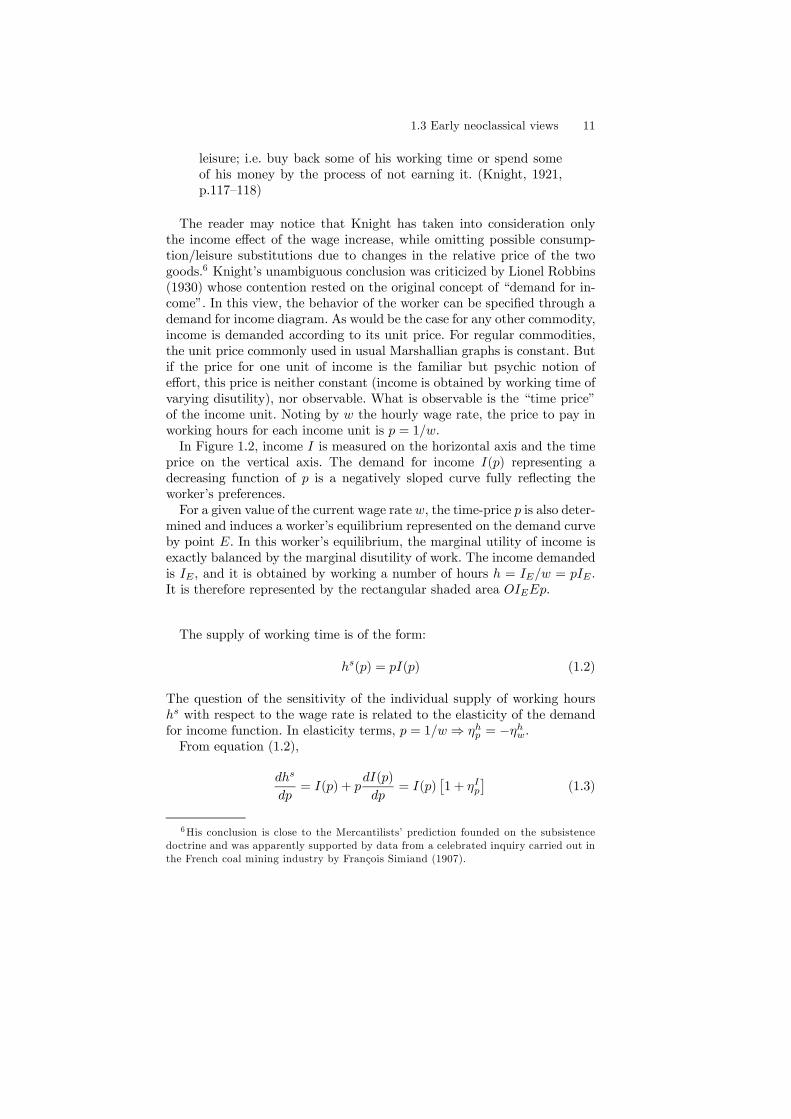
The reader may notice that Knight has taken into consideration onlythe income effect of the wage increase, while omitting possible consump-tion/leisure substitutions due to changes in the relative price of the twogoods.6 Knight’s unambiguous conclusion was criticized by Lionel Robbins(1930) whose contention rested on the original concept of “demand for in-come”. In this view, the behavior of the worker can be specified through ademand for income diagram. As would be the case for any other commodity,income is demanded according to its unit price. For regular commodities,the unit price commonly used in usual Marshallian graphs is constant. Butif the price for one unit of income is the familiar but psychic notion ofeffort, this price is neither constant (income is obtained by working time ofvarying disutility), nor observable. What is observable is the “time price”of the income unit. Noting by w the hourly wage rate, the price to pay inworking hours for each income unit is p = 1/w.In Figure 1.2, income I is measured on the horizontal axis and the time
price on the vertical axis. The demand for income I(p) representing adecreasing function of p is a negatively sloped curve fully reflecting theworker’s preferences.For a given value of the current wage rate w, the time-price p is also deter-
mined and induces a worker’s equilibrium represented on the demand curveby point E. In this worker’s equilibrium, the marginal utility of income isexactly balanced by the marginal disutility of work. The income demandedis IE , and it is obtained by working a number of hours h = IE/w = pIE .It is therefore represented by the rectangular shaded area OIEEp.
The supply of working time is of the form:
hs(p) = pI(p) (1.2)
The question of the sensitivity of the individual supply of working hourshs with respect to the wage rate is related to the elasticity of the demandfor income function. In elasticity terms, p = 1/w⇒ ηhp = −ηhw.From equation (1.2),
dhs
dp= I(p) + p
dI(p)
dp= I(p)
£1 + ηIp
¤(1.3)
6His conclusion is close to the Mercantilists’ prediction founded on the subsistencedoctrine and was apparently supported by data from a celebrated inquiry carried out inthe French coal mining industry by François Simiand (1907).

12 1. Brief history of working time theory
p
IIncome0
Demand for income
Hours-price of theincome unit
I(p)
E
IE
FIGURE 1.2. Demand for income and total hours supply
where ηIp stands for the elasticity of the demand for income with respect
to its unit pricedI
dp
p
I.
Therefore, ηIp < (−1) ⇒ ηhp < 0 and ηhw > 0. The individual supplyelasticity of working time ηhw is therefore positive if η
Ip < (−1), negative if
ηIp > (−1).Lionel Robbins’ interpretation is attractive since it is performed in the
familiar terms of demand schedules and critical elasticities analogous to theterms involved in the famous King law. It is compatible with different shortrun labor supply behaviors which were to be more thoroughly explainedin terms of indifference curves and income and substitution effects in thesubsequent development of neoclassical thought (see Chapter 4).
1.4 Conclusion
As this first chapter sets out to confirm, working time is a permanent topicin economic analysis, closely linked to the notion of worker’s welfare, evenif this latter concept was initially perceived as a subsistence limit. The suc-cessive doctrines related to the elements of labor contract clearly depend onmore or less arbitrary selections of axioms in the representation of basic cir-cumstances in which labor relations are formed. The Mercantilists allowedfor some form of competition among firms, and scarcity of workers enabledthem to impose their preferred working time. This optimum working timerests on specific implicit assumptions in terms of the individual preferencesof the workers. The Classics switched to an opposite negotiation context

1.4 Conclusion 13
in which a structural excess supply of workers tends to empty the worker’schoice and drive down wages to the subsistence level, giving no expressionto individual consumption/leisure preferences. Marx attempted to give ageneral status to his analysis of a special case, in which the market forworking hours yields to a market for labor power. The precise conditionfor the stability of this form of exchange in terms of market structures,individual and collective behavior were not clearly enunciated.Traditional neoclassical writers introduced a more explicitly axiomatic
form of thought and gave more details about their representation of mar-ket structures, preferences, productive techniques and individual behavior.The most sanguine of them developed an idealized vision of the economy,in which flexible prices — including wage rates — eliminate all forms of ra-tioning such as joblessness or overwork. Such an optimistic view may beobtained only at the price of overstating the realm of perfect competition,overlooking intrinsic features of labor cost structure and time varying work-ers’ effectiveness, as well as neglecting the role of limited information andof collective bargaining in labor relations.Modern working time analysis should take into consideration the essential
features of contemporary labor markets. After presenting the main observedstylized facts and policies, this text will build on several theoretical analysesin a more general framework.

14 1. Brief history of working time theory

This is page 15Printer: Opaque this
2Basic facts
Over the twentieth century, the recorded yearly average number of hoursworked per employee has steadily declined in most countries of the indus-trialized world.However, since the early eighties, this trend has faded and even reversed
in some countries. Whereas working time was rather uniformly distributedamong the main industrializing countries in the first decade of the century,the recent evolution in the nineties has introduced more variety, and devi-ations are tending to increase from one country to another. For instance,although worked hours continue to decline steadily in the Netherlands,they have slightly increased in the United States, Sweden and Finland, andstabilized in France.A wide range of durations now prevails in observed working time. A
working week of 40 hours is still the current norm in most economies ofthe Western world, but the fraction of employees actually working 40 hoursis falling. In many countries, the respective proportions of people workingvery short and very long hours have increased, contributing to increaseddomestic variance.Part-time jobs in particular have become common in many countries.
While this development may reflect a choice by employees in some cases, itis also often interpreted as a consequence of the need for more varied andflexible arrangements expressed by employers having to cope with stringentconstraints imposed by technology and customers.At a more subjective level, it must be said that a lot of surveys tend to
confirm that many employees are in some sense not satisfied with the actual

16 2. Basic facts
duration of their work; but the nature of this rationing is not uniform, sincesome of them wish to work more for the going hourly wage, and others less.
2.1 Trends in working hours
As is well known, in the first factories established in Manchester and inthe neighboring towns of Lancashire, at the end of the eighteenth century,working time was extremely long. According to Bienefeld (1972), the repre-sentative textile factory used to operate 69 hours per week at the beginningof the nineteenth century, extending its working week to the bewilderingscore of 72 hours in 1830. By mid-century, textile firms still demandedbetween 58 to 60 hours (10.5—11 hours of work per day from Monday toFriday and 3—7 hours on Saturday). Such orders of magnitude must be keptin mind when considering the weekly standard of 40 hours recorded todayin the greatest part of the developed world.Maddison (1995) brings into the picture some interesting evidence per-
taining to the long term trend (1870-1992) in hours per worker (Table2.1). For more than a hundred years, the trend in annual hours has beenclearly downward sloping, but with large discrepancies between countries.This downward trend was reinforced after the Second World War, with thenotable exception of Japan, where working hours reached a peak in 1960.
YEAR Canada France W. Ger. Italy Japan UK US1870 2964 2945 2941 2886 2945 2984 29641890 2789 2770 2765 2714 2770 2807 27891913 2605 2588 2584 2536 2588 2624 26051929 2399 2297 2284 2228 2364 2286 23421938 2240 1848 2316 1927 2391 2267 20621950 1967 1926 2316 1997 2166 1958 18671960 1877 1919 2081 ... 2318 1913 17951973 1788 1771 1804 1612 2042 1688 17171987 1673 1543 1607 1528(a) 2020 1557 16081992 1656 1542 1563 1490 1876 1491 1589
TABLE 2.1. Annual hours worked per person employed, 1870-1992. Source: Mad-dison (1995). (a) 1985
It is worth mentioning that in the same interval 1870—1992, estimatesof per capita GDP have been multiplied by a factor close to ten (Maddi-son, 1995). Since the share of wages in output remained rather constantthroughout the interval, one may infer that, in the long run, this fall in
2.1 Trends in working hours 17
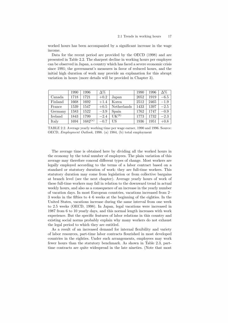
worked hours has been accompanied by a significant increase in the wageincome.Data for the recent period are provided by the OECD (1998) and are
presented in Table 2.2. The sharpest decline in working hours per employeecan be observed in Japan, a country which has faced a severe economic crisissince 1991; the government’s measures in favor of reduced hours, and theinitial high duration of work may provide an explanation for this abruptvariation in hours (more details will be provided in Chapter 3).
1990 1996 ∆% 1990 1996 ∆%Canada 1718 1721 +0.2 Japan 2052 1919 −6.5Finland 1668 1692 +1.4 Korea 2512 2465 −1.9France 1539 1547 +0.5 Netherlands 1433 1397 −2.5Germany 1583 1522 −3.9 Spain 1762 1747 −0.9Ireland 1843 1799 −2.4 UK(b) 1773 1732 −2.3Italy 1694 1682(a) −0.7 US 1936 1951 +0.8
TABLE 2.2. Average yearly working time per wage earner, 1990 and 1996. Source:OECD, Employment Outlook, 1998. (a) 1984, (b) total employment
The average time is obtained here by dividing all the worked hours inthe economy by the total number of employees. The plain variation of thisaverage may therefore conceal different types of change. Most workers arelegally employed according to the terms of a labor contract based on astandard or statutory duration of work: they are full-time workers. Thisstatutory duration may come from legislation or from collective bargainsat branch level (see the next chapter). Average yearly hours of work ofthese full-time workers may fall in relation to the downward trend in actualweekly hours, and also as a consequence of an increase in the yearly numberof vacation days. In most European countries, vacations increased from 2—3 weeks in the fifties to 4—6 weeks at the beginning of the eighties. In theUnited States, vacations increase during the same interval from one weekto 2.5 weeks (OECD, 1998). In Japan, legal vacations were increased in1987 from 6 to 10 yearly days, and this normal length increases with workexperience. But the specific features of labor relations in this country andexisting social norms probably explain why many workers do not exhaustthe legal period to which they are entitled.As a result of an increased demand for internal flexibility and variety
of labor resources, part-time labor contracts flourished in most developedcountries in the eighties. Under such arrangements, employees may workfewer hours than the statutory benchmark. As shown in Table 2.3, part-time contracts are quite widespread in the late nineties. (Note that most

18 2. Basic facts
definitions of part-time contracts changed between 1979 and 1996, thusdata in the respective columns cannot serve for direct comparisons.)
1979 1996 1979 1996Canada 13.8 18.9 Japan 15.4 21.8Finland 6.6 7.9 Netherlands 16.6 36.5France 8.1 16.0 Sweden 23.6 23.6Germany 11.4 15.1(a) UK 16.4 22.2Italy 5.3 5.4 US 16.4 18.3
TABLE 2.3. Part-time workers as a percentage of total employment according tonational definitions. Source: OECD, Employment Outlook, 1998. (a) 1993
Average yearly hours per incumbent worker may vary under the influenceof changes in the number of hours included in the full-time contract or as aconsequence of a varying proportion of part-time workers in the economy.Table 2.4 attempts to summarize these simultaneous influences.
As can be seen, in most cases both the decrease in the average annualhours of the full-time workers and the increase in the number of part-timejobs have contributed to the downward trend in average working hoursduring the century.It would be interesting to further analyze the two idiosyncratic situations
of the United States and Sweden. In the latter, the positive variation islargely due to increased hours included in part-time contracts, stronglyweighted by a large number of women participating in the labor market,and to a significant fall in absenteeism after the last recession (Anxo, 1995).In the case of the United States, the data have sometimes been displayed
in apparently contradicting terms. Schor (1991, p.1) claims that: “in thelast twenty years the amount of time Americans have spent at their jobs hasrisen steadily... Working hours are already longer than they were forty yearsago”. This particular account has not found much support in subsequentor alternative enquiries. In a thorough and detailed study, Coleman andPencavel (1993) showed that between 1940 and 1988 the annual averageworking time per worker has been “virtually constant”. McGrattan andRogerson (1998) find that between 1950 and 1990, average weekly hours perworker in the United States fall from 40.71 to 36.64. Many other relevantdetails pertaining to working hours patterns and disaggregated tendenciesmay be found in these two last references.Many proponents of a mandatory reduction in working time have in mind
some idea of work-sharing. In a preliminary empirical approach, it can besaid that a definite negative relationship between employment and working

2.1 Trends in working hours 19
Overallchangeinhours
(1+2+3)
Changein hours(full-timeworkers)(1)
Changein hours(part-timeworkers)(2)
Changeinshare ofpart-timeworkers(3)
Belgium 1983—93 -7.5 -2.5 0.2 -4.9Canada 1983—93 -1.1 0.7 0.5 -2.3Denmark 1985—93 -6.6 -7.1 -0.9 1.4France 1983—93 -4.1 0.4 0.7 -4.4Germany 1983—93 -10.9 -6.1 -0.9 -3.9Greece 1983—93 -1.0 -1.6 -0.4 1.3Ireland 1983—93 -7.4 -1.0 -0.4 -6.0Italy 1983—93 -3.7 -3.0 0.4 -0.9Luxemburg 1983—93 -2.1 -0.9 -0.1 -1.1Netherlands 1987—93 -6.6 0.0 3.2 -11.3Portugal 1983—93 -6.9 -6.5 0.6 -0.3Spain 1987—93 -6.0 -3.8 -0.4 -1.8Sweden 1987—94 7.7 1.8 3.6 2.3UK 1983—93 -1.5 3.8 -0.5 -5.0US 1983—93 7.3 4.7 1.3 1.2Average (all) 1983—93 -3.1 -1.4 0.5 -1.7
TABLE 2.4. Contributions of various factors to recent changes in average annualhours of employees. Source: OECD, Employment Outlook, 1998
hours would provide major support in favor of this policy. The followinggraphs display working hours and employment for five countries on thebasis of the ILO Yearbook of Labor Statistics, 1997.
37.5
38
38.5
39
39.5
40
40.5
41
41.5
42
42.5
1977
1979
1981
1983
1985
1987
1989
1991
1993
1995
20800
21000
21200
21400
21600
21800
22000
22200
22400
22600
22800
hoursemployment
Working hours and employment in France, 1977—1996

20 2. Basic facts
36
37
38
39
40
41
42
43
1977
1979
1981
1983
1985
1987
1989
1991
1993
23000
24000
25000
26000
27000
28000
29000
hours
employment
Working hours and employment in West Germany, 1977—1993
39.2
39.4
39.6
39.8
40
40.2
40.4
40.6
40.8
1987
1988
1989
1990
1991
1992
1993
1994
1995
1996
23500
24000
24500
25000
25500
26000
26500
27000
27500
hoursemployment
Working hours and employment in the United Kingdom, 1987—1996

2.1 Trends in working hours 21
41.0
42.0
43.0
44.0
45.0
46.0
47.0
48.0
1978
1980
1982
1984
1986
1988
1990
1992
1994
1996
48000
50000
52000
54000
56000
58000
60000
62000
64000
66000
hours
employment
Working hours and employment in Japan, 1977—1996
33
33.5
34
34.5
35
35.5
36
36.5
1977
1979
1981
1983
1985
1987
1989
1991
1993
1995
0
20000
40000
60000
80000
100000
120000
140000
hours
employment
Working hours and employment in the United States, 1977—1996
Inspection of these graphs unfortunately gives little help in determin-ing whether working time and employment are negatively correlated. Inthe United Kingdom, the two series seem to be positively correlated, inWest Germany and Japan negatively correlated, in France and the UnitedStates only loosely correlated. In Japan, the abrupt fall in hours may havecushioned the rise in unemployment during the current crisis.

22 2. Basic facts
2.2 Hours of work: structure
In most countries, the standard duration of work is close to 40 hours perweek, and men work longer days than women (OECD, 1998). There areimportant differences between countries, as emphasized by Eurostat, theEuropean statistical office (Table 2.5).
Hours per week: 1—35 36—39 40 41—45 46+ TotalEurope 15 8.1 31.4 32.2 8.9 19.4 100%Germany 8.2 38.9 34.7 4.1 14.1 100%France 7.6 61.5 8.4 8.8 13.7 100%Italy 10.3 20.4 40.8 7.9 20.6 100%Netherlands 1.2 35.4 50.9 1.6 10.9 100%Spain 6.0 8.9 60.7 7.2 17.2 100%Sweden 2.8 13.5 67.6 6.5 9.6 100%UK 9.1 21.9 13.8 20.1 35.1 100%
TABLE 2.5. The pattern of weekly working time in 1997, selected Europeancountries (full-time employees; actual hours per week). Source: Labor Force Sur-vey 1997, Eurostat (1998)
Hours of work also vary according to the activity sector and the socio-professional category. According to the Eurostat Labor Force Survey (1998),in the Europe of 15, actual hours of work were in 1997 the highest in agri-culture (44.8 hours) and lowest in the service sector (39.7) and in manu-facturing (36.8 hours).Nobody would be surprised to learn that executives work the longest
hours. Less easy to explain is the relatively reduced weekly hours of theless qualified people, as shown in Table 2.6. This pattern is valid throughoutthe European region (Greece excepted); the most striking situation is in theNetherlands, where average weekly working time of less-qualified workersis only 23.0 hours.
The same pattern applies to the United States economy. According toRones at al. (1997), in 1993, 45% of the managers and sales persons per-formed over 49 hours per week (as compared with a 40 hours statutoryweek); on the other hand, only 16% of the less qualified employees worksuch a long time.Analyzing the trends of working hours, Coleman and Pencavel (1993)
report that since 1940, hours fell for those with relatively little schoolingand rose for well-educated people. As they mentioned, “a rising trend in thework hours of the well-educated also squares with reports of longer hours

2.3 Do people think they work too much? 23
France Ger. Italy UK EU-15Managers and administrators 44.6 43.4 41.4 45.6 43.9Academic and scientificprofessions
35.6 38.2 29.7 40.2 36.6
Associated professionaland technical
37.1 36.1 38.1 38.9 36.9
Clerical and secretarial 35.5 34.2 37.2 33.5 35.1Selling 35.0 33.0 38.3 27.7 33.2Agricultural and fishingworkers
37.2 39.2 38.7 37.1 38.9
Craft and related 38.8 38.4 40.0 43.8 39.7Plant and machine operatives 39.0 39.2 39.9 44.0 40.2Unskilled workers 31.5 31.1 36.6 29.9 32.4Armed forces 45.9 41.1 ... 45.3 42.4Total 36.7 36.3 37.4 37.4 36.8
TABLE 2.6. Wage earners: average weekly hours per socio-professional categoryin 1997. Source: Labor Force Survey 1997, Eurostat (1998)
among professional and managerial workers” (Coleman and Pencavel, 1993,p.282).Costa (1998) points to the recent tendency of low-paid workers to do
fewer hours than highly-paid workers, as compared to the relatively longhours done by the same category of wage earners at the end of the nine-teenth century (Table 2.7). The author comments that the largest declinein hours worked took place before 1973, probably in the 1920s. The bulkof the reduction is attributable to low wage-earners.1
2.3 Do people think they work too much?
Workers’ preferences are undoubtedly an important factor accounting fordifferences between countries with respect to working hours pattern. A firstattempt to infer such preferences is based on surveys. As will soon be madeclear, different statistics often seem to contradict one another.In 1989, the International Social Survey Programme (ISSP) organized a
survey among the OECD countries. They asked every individual: “Thinkof the number of hours you work and the money that you make in yourmain job, including regular overtime. If you had only one of three choices,
1Costa (1998) argues that the observed shift in hours is due to a large extent tochanges in the supply, as opposed to changes in the demand for hours resulting fromtechnological improvements.

24 2. Basic facts
hourly wage deciles 1890s 1973 1991<10 (bottom) 10.99 8.83 8.0510—20 10.46 8.47 8.4720—30 10.50 8.54 8.5330—40 10.63 8.38 8.6140—50 10.31 8.34 8.5950—60 9.99 8.33 8.6160—70 10.29 8.33 8.4770—80 10.07 8.32 8.6680—90 9.64 8.26 8.64>=90 (top) 8.95 8.22 8.72
90th/10th 0.81 0.93 1.0890th/50th 0.90 0.99 1.0150th/10th 0.94 0.94 1.07
TABLE 2.7. Distribution of usual-length work day by hourly wage deciles, Amer-ican men aged 25-64. Source: Costa (1998) who used data from the US Bureauof Statistics surveys in the 19th century
which of the following would you prefer: (1) work longer hours and earnmore money, (2) work the same number of hours and earn as much money,(3) work fewer hours and earn less money”. A summary of the answers —as a percentage of total answers — is presented in Table 2.8.
Answer:more hoursmore pay
same hourssame pay
fewer hoursless pay
Austria 22.59 71.53 5.88Germany 13.50 76.41 10.09Italy 31.03 62.43 6.53Ireland 30.37 64.64 4.99Netherlands 17.54 70.16 12.29Norway 24.36 68.70 6.93UK 23.77 68.05 8.17US 32.67 61.83 5.51
TABLE 2.8. Preferred working time and income. Percentage of total answers.Source: Bell and Friedman (1994)
According to this survey, in many countries, about one third of the em-ployees are not satisfied with present hours of work; it is worth noticingthat the unsatisfied would, in general, prefer to increase working hours; the

2.3 Do people think they work too much? 25
Netherlands appears to be the country with the largest minority of workersdesiring to work less.Kahn and Lang (1996a, 1996b) mention several surveys carried out in the
eighties in the United States and Canada which show that approximatelyhalf of all workers would like to work a different number of hours perweek if they could continue to receive their usual hourly wage. About twothirds of the rationed workers would like to work more hours and only onethird would like to work fewer hours. Drolet and Morissette (1997) presentthe results of the Survey of Work Arrangements held in November 1995by Statistics Canada: two thirds of paid workers in Canada declared theywere satisfied with their work hours; 27% favored more hours for more payand only 6% preferred fewer hours for less pay. This pattern is robust as itholds for each of the ten provinces, age group, education level, industrialand professional group.As indicated by a number of opinion polls, the North American pattern,
with workers wishing to work more at the going wage rate, seems to havealso prevailed in the eighties in Japan (Takagy, 1993).The European Commission organized various ad hoc labor market sur-
veys, covering inter alia working time issues, in 1984, 1989 and 1994. Aquestionnaire was addressed to over 10 000 employees in all sectors of theEU. An interesting question was: “Assuming that the present hourly wagerate remained unchanged, would you like to work less, as long or longer?”Table 2.9 pinpoints the tendency of European workers to work shorterhours, a result that seems at odds with the ISSP query. However, the factthat 21% would like to work longer hours cannot be neglected: obviously,worker rationing goes both ways, even though overwork seems to be pre-vailing in this survey.
1989 1994Total 100% 100%Answer :- less 37 29- as long 51 48- longer 8 21- no reply 4 2
TABLE 2.9. Preferred working time (overall). Source: European Commission(1995)

26 2. Basic facts
The tendency is stable throughout Europe (Table 2.10), with the notableexception of France, where 67% of the respondents would like to workmore.2
Country Answer:(actual hoursa) Total: Less As long Longer No replyW. Germany(1552)
100% 30 62 7 1
France(1520)
100% 21 11 67 1
Italy(1682)
100% 29 50 17 4
Netherlands(1395)
100% 21 67 12 0
Spain(1746)
100% 32 52 12 4
UK(1728)
100% 33 53 13 1
TABLE 2.10. Preferred working time, selected countries, 1994. Source: EuropeanCommission (1995). (a) Pro memoria: actual yearly working hours per employedperson (in UK, hours per wage earner)
Inference from such surveys is difficult since, when asked “If the choicewere offered at the next wage round between an increase of pay for thesame hours of work and shorter working time for the same pay you get now,which would you prefer?”, most people prefer the pay increase, even if inanswer to the former question they had declared that they would prefer lesshours (Table 2.11). Most European countries stick to this pattern, with thenotable exceptions of Denmark and the Netherlands which favored workingtime reductions.
Of course, the results of such enquiries should be interpreted very cau-tiously, since the answers are highly sensitive to external factors, such asthe general economic and political environment, the economic cycle, the
2 In a special study devoted to the UK labor market and based on data from theBritish Household Panel Survey (BHSP) of 1991, Stewart and Swaffield (1997) foundthat most male British workers are subject to overwork. They estimate a mean value ofdesired working time by manual men of 43 hours per week, less than actually performedby this category of workers.
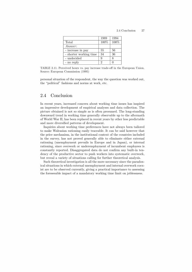
2.4 Conclusion 27
1989 1994Total 100% 100%Answer :- increase in pay 55 56- shorter working time 34 36- undecided 9 8- no reply 2 0
TABLE 2.11. Perceived hours vs. pay increase trade-off in the European Union.Source: European Commission (1995)
personal situation of the respondent, the way the question was worked out,the “political” fashions and norms at work, etc.
2.4 Conclusion
In recent years, increased concern about working time issues has inspiredan impressive development of empirical analyses and data collection. Thepicture obtained is not so simple as is often presumed. The long-standingdownward trend in working time generally observable up to the aftermathof World War II, has been replaced in recent years by other less predictableand more diversified patterns of development.Inquiries about working time preferences have not always been tailored
to make Walrasian rationing easily traceable. It can be said however thatthe price mechanism, in the institutional context of the countries includedin the survey, has not proved generally able to eliminate either externalrationing (unemployment prevails in Europe and in Japan), or internalrationing, since overwork or underemployment of incumbent employees isconstantly reported. Disaggregated data do not confirm any built-in ten-dency of the productive sector to push workers into systematic overwork,but reveal a variety of situations calling for further theoretical analysis.Such theoretical investigation is all the more necessary since the paradox-
ical situations in which external unemployment and internal overwork coex-ist are to be observed currently, giving a practical importance to assessingthe foreseeable impact of a mandatory working time limit on joblessness.

28 2. Basic facts

This is page 29Printer: Opaque this
3Working time policy: an overview
3.1 Why regulate working time?
From material presented in Chapter 2, it appears that during the twentiethcentury, recorded hours of work have steadily and considerably decreasedthroughout the industrialized world. This fall might be interpreted as aspontaneous development in an increasingly decentralized economic system,within a general equilibrium framework, since both supply and demand con-siderations are able to account for a downward trend. State interventioncould also have influenced this outcome. The rationale for government in-terference in working time determination exists and has been inspired overtime by varying conceptions and objectives.The role of law in this matter was first intended to protect the workers
from excessive working days judged detrimental to their health and welfarein the long run. Such overwork preoccupations seem to have prevailed inWestern Europe from the middle of the nineteenth century to the recon-struction era in the aftermath of World War II. Throughout this period,increasingly protective limits were imposed first by the British Parliament,often followed in particular by the regulations devised in continental Eu-rope.1
Assuming perfect competition in a pure Walrasian interpretation of eco-nomic life, these rules can be understood as protecting the workers against
1For instance, the notion of a fixed working week and a standard weekend restingtime was establised in Britain by 1890 or so (Cross, 1989).

30 3. Working time policy: an overview
themselves, since actual working time, considered as a market equilibriummagnitude, is supposed to reflect their own preferences (for details, seeChapter 4). The market sector of the economic machinery destroys leisureor home production, in order to produce marketable goods and services.To justify state intervention, we have to think that under the rule of freemarket forces, this process goes too far. Short-sighted workers may not beable to fully evaluate the global effect of long working hours on health orpersonal development. In this case, the government, as guarantor of thepublic interest, is entitled to overrule the system and superimpose its con-sumption/leisure preferences on those of the workers.As we have seen in Chapter 1, according to the interpretation of Karl
Marx, working time limits would protect the workers against the employers’greed for profits. Some neoclassical writers themselves have referred to thebounded rationality of employers, unable to realize that, due to exertion orother efficiency considerations, shorter working days do not necessarily im-ply substantially reduced output.2 In such a case, equilibrium working timedoes not sustain the economic system in a Pareto-optimal configuration.Limited rationality of workers, unable to understand their long term
welfare requirements, or limited rationality of employers, overestimatingthe consequences on output of reduced working time, have been, and stillare, alleged foundations for the regulation of working hours.In periods of high unemployment however, such welfare considerations
tend to be overshadowed by the more pragmatic goal of job creation ob-tained from a hypothetical man-hours substitution process. For instance,during the Great Depression, this idea was widely circulated. As early as1933, the International Labor Office considered a proposal by the Italiangovernment advising a uniform hours standard intended to reduce compe-tition and to reabsorb unemployment. Trade unions fiercely called for a 40hour week, and, like today, required that no wage cut should accompanythe reduction of hours (Cross, 1989).More recently, in particular after the second oil shock, faced by high and
persistent unemployment, a number of governments have resorted againto working time regulations which were perceived as a politically sustain-able way to create or defend jobs.3 Most often, these policies are groupedtogether under the term of “work-sharing”, which can be defined as anypolicy involving a redistribution of employment through a reorganizationof working time. Some measures, like a general reduction in working hours,voluntary part-time working and job sharing, aim at reducing daily orweekly hours of work. These measures might foster the demand for workersonly if the technological process and cost structures are such that profit
2 See the comment of John Hicks (1932) on the concept of “optimal working day”.3Additional and more detailed information on working time policies can be found in
the OECD 1998 Employment Outlook, the Policy Bulletin of the European EmploymentObservatory and the 1999 issues of the European Industrial Relations Review.
3.2 Work-sharing methods in international comparison 31
maximizing firms tend to compensate the law induced scarcity of availablehours by new hires. However, in some cases, this substitution is not feasi-ble in the short run; some other longer term measures such as paid-leavearrangements, career break or early retirement may be attempted, not be-ing subject to the same shortcomings. In this case, firms would be morelikely to replace an incumbent worker who leaves the firm (temporarily ordefinitively) by a new one.
3.2 Work-sharing methods in internationalcomparison
The general reduction in working hours is probably the most intuitivelyappealing work-sharing method; during the last two decades it has benefitedfrom significant popular support, especially in countries plagued by highunemployment.The typical work-sharing regulation involves limitations on working hours
for all workers, most often with the declared objective of creating jobs. Suchregulations are often based on three elements: statutory working hours (ingeneral a weekly norm beyond which an overtime premium wage is due), anovertime premium to be paid for hours longer than the statutory level and aquota of maximum permitted overtime hours (on a weekly or yearly basis).Such reductions may be negotiated between workers and the trade unionsor may be imposed by law. For instance, throughout the nineties, Germantrade unions have successfully pushed for a reduction of the statutory work-ing week to 35 hours. During the same period, in Japan, the governmentalsupport for a reduced 40 hour working week has finally shifted the balancein favor of the trade unions, which have also succeeded in reducing workingtime in the last few years. In France, a law passed in 1998 set up a methodfor introducing a statutory 35 hour week by 2002 at the latest. The Italiangovernment is seriously considering a similar move. In 1999, unions in Fin-land, Greece, Spain, Sweden, Belgium and Switzerland are advocating asimilar policy (they are in general silent on the possibility of a consecutivereduction in the wage bill that should accompany the reduction in hours).More details on the policy of working time reduction will be presented inthe next section, containing three country cases.Some countries have encouraged voluntary part-time working, imple-
menting various incentives intended to prompt workers to reduce theirworking hours, while encouraging employers to hire replacement workers.This method is very popular in the Netherlands where the governmentstrives to guarantee part-timers equal treatment with full-timers. In Bel-gium, the government introduced in 1994 an incentive grant for employeesaccepting a move from a full-time to a part-time job. In 1997, the law wasfurther extended: workers reducing their working time by at least 20% and

32 3. Working time policy: an overview
up to 50% are entitled to a two-year incentive grant proportional to the ex-tent of the working time reduction. In Austria, under the Solidarity Model(1998), employees reducing their working hours and the replacement work-ers hired are entitled to a solidarity premium for a period of up to two yearsfrom the date of recruitment of the latter; this premium is equivalent to ashare of the unemployment benefits pro rata to the extent of the workingtime reduction. In some countries, employers must pay a fixed contributionper employee (for public health, pensions, unemployment benefits), at leastunder a certain wage-income threshold. Such a practice is obviously detri-mental to the extension of part-time jobs. Consequently, many attemptshave been recorded lately, aiming at replacing such thresholds with con-tributions proportional to the wage income, sometimes coupled with anexemption for low wage workers (in Canada, Finland and France).Job sharing in a strict sense is a special part-time arrangement where
two persons share the tasks of a full-time job, dividing the full-time wageon a proportional basis. While this practice has developed in the last fewyears, only Finland has passed a law to organize such deals.One recent innovation in the realm of work-sharing policies in Germany
was the adoption in 1996 of a part-time early retirement scheme. Underthis regulation, older workers are encouraged to work on a part-time basis,in order to push firms to recruit younger people. Employees aged over 55may cut working time by 50% for a five-year maximum period. They willbe paid by the firm on the basis of their actual hours, but the governmentwill reimburse 20% of their pay and pension contributions if employers alsoaward a further 20% of pay and recruit young people.In some other cases, work-sharing is not considered in relation to short
lapses of time (day or week) but in a life-cycle perspective. In this approach,some employees, deemed more able to cope with joblessness are encouragedto leave, and firms are encouraged to replace them with unemployed per-sons. For instance, under paid-leave arrangements, workers take extendedperiods of paid leave, most often with a vocational training objective, withunemployed people being recruited to replace them. In Austria, employ-ees may take a six month to one year training leave, without pay; duringthis period they may benefit from a training indemnity, proportional tothe parental indemnity. Other countries like Belgium, the Netherlands orFinland have taken the same steps. Career breaks refer to workers takingperiods of unpaid leaves, for various reasons (care for children, undertakinga trip, etc.). Many countries have set up early retirement schemes, whereworkers near the retirement age are allowed to cease work with a reducedpension during the intermediate years. In such cases, working time policydoes not purport to create new jobs but only aims at redistributing the jobrationing among different subpopulations.As will be seen in the following chapters, this text focuses on the choice
of working time defined in a short period interpretable as a day or a week;therefore, the later analytical chapters will place special emphasis on work-

3.3 Working time reduction: three country cases 33
ing hours regulation, in particular on the general reduction in working timeand on the ability of this measure to increase employment.
3.3 Working time reduction: three country cases
General reductions in working hours are often very popular policies; whilestrongly opposed by firms, they benefit from significant public support inmany developed countries. Trade unions also back them, or at least a specialvariant, where reduction in working hours is to be achieved with a constantwage bill. In this case, the impact on the economy is not simple, since thesuggested measure implies simultaneously a new value of the working timeconstraint and an increase of the hourly wage rate. Policy makers are thusin the difficult situation of arbitrating between the various social partners.Three country cases allow us to highlight the complex character of publicdecisions intended to support work-sharing policies, in particular by meansof a general reduction in working hours. We choose three countries wherethe work-sharing paradigm seems to be particularly influential.
3.3.1 France: reducing working time by law
Like many other developed countries, France inherited a legal system aim-ing at protecting the workers from excessive burdens, essentially throughweekly hours limits and overtime premium constraints imposed on employ-ers.4
In the context of the global economic slump in the early 1980s, theFrench Parliament, however, decided in 1981 that the statutory workingtime should be reduced from 40 to 39 hours per week, with an overtimewage fixed at 1.25 of the regular rates. The law also introduced a fifth weekof paid vacation and reduced the retirement age from 65 to 60 years. Themaximum overtime was limited to 130 hours per year. Unfortunately, thelaw did not prove able to curb soaring unemployment and the followinggovernments gave up the idea of mandatory reduction of working time.5
They finally adopted a more flexible policy also aiming at reducing hours,but by means of powerful incentives.In general, regulations passed after 1981 granted the firms agreeing to
reduce the duration of work substantially alleviated social contributions,contingent upon maintaining or increasing employment. In some sense, this
4The French passed a first working time regulation in 1848, when the maximum dailyduration was set at 12 hours.
5According to an empirical analysis by Crépon and Kramarz (1999), workers whowere working 40 hours a week in March 1981 (when the reduction was decided) are lesslikely to be employed in 1983, than identical workers who, in 1981, were working 39hours.

34 3. Working time policy: an overview
type of regulation aimed at internalizing the social cost of joblessness. Thefirms able to create jobs by working time reduction are given a share of thesavings they induce in favor of the unemployment compensation budget.The most important incentive program was laid down in June 1996 (“LoiRobien”). Firms which simultaneously reduce the duration of work (by10%) and hire, benefit from a significant social charge credit (amountingto 30—40% of the employer’s contribution). This labor cost reduction isgranted for a rather long activity interval, up to seven years (Freyssinet,1997). Although there was no obligation for firms and workers to engagein negotiations under the terms of this law, by the end of June 1998, some2900 agreements had been signed under this regulation, covering 278 000workers and creating or safeguarding 15 500 jobs, according to the FrenchMinistry of Employment and Solidarity.As the early results of this law seemed rather short of its expected ben-
efits — unemployment in France was still very high (11.8% in May 1998)— the socialist government embarked on an active process inspired by thework-sharing paradigm, more dirigiste and more in the spirit of the 1981law. The so-called “Loi Aubry” of June 13, 1998 and the correspondingimplementation decrees simultaneously set a new weekly norm (35 hoursper week), imposed a method (compulsory collective bargaining) and intro-duced accompanying measures, mainly public support for the most diligentfirms.The law fixes the statutory working week at 35 hours as of January 1,
2000 for firms with more than 20 workers and as of January 1, 2002 forall firms. It is important to note that the figure of 35 hours representsthe statutory, not the obligatory, working time: firms are allowed to hireworkers for more than 35 hours, but must pay the higher wage rate for thisextra time (1.25 times the normal rate).6
Having established this norm, the law requires enterprises to bargainwith their respective social partners (in most cases, trade unions) overthe conditions under which the reduction is to take place. Negotiationson working time must be carried out at the level of the firm, but in somecases, branch or national level negotiations can also take place. In addition,a company is entitled to a five-year tax credit if it cuts working hours byat least 10% and creates jobs or avoids redundancies of at least 6% of itsworkforce.According to a report by the French Ministry for Employment and Soli-
darity, on July 21, 1999 more than 11 500 firm level agreements had beensigned on working time, covering almost two million employees. At branchlevel, 101 agreements had been concluded by July 1999.7 In many sectors,
6By June 1999, the government proposed some inflection to the initial text. Hence,firms will benefit from a one-year transition period, during which the wage premium onweekly hours exceeding the 35 and below 39 will be only 10% (instead of 25%).
7For information update, see http://www.35h.travail.gouv.fr.

3.3 Working time reduction: three country cases 35
the government judged them consistent with its objectives of supportingemployment and decided on their extension to all firms of the branch.However, the most important adopted branch agreement was also the
most litigious. With 1.8 million employees and a turnover close to $37billion, the engineering branch is the most important industrial activity inFrance. An agreement was signed in July 1998 between UIMM, the employ-ers’ union and three main worker trade-union confederations (FO, CFTC,CGC). As requested, the statutory working time will become 35 hours perweek, but the number of authorized overtime hours was extended from 94hours to 180 hours per year and worker. Overtime can be compensated ei-ther by holidays in the subsequent period or by extra wages. Furthermore,the 35 weekly hours imply a reference annual period of 1645 hours, withfirms able to vary weekly hours at their convenience within an upper limitof 10 daily hours. Also, the agreement lays down the possibility of spe-cial labor contracts establishing a lump-sum payment for predeterminedtasks, independently of the implied working time. Many other sectors havenow applied for extensions of this particular agreement. For the time being,the government has refused to acknowledge them, on the grounds that suchagreements will not boost the demand for workers. Somewhat ironically, thelaw triggered a bargaining process ending in an agreement finally grantingmore flexibility to the firms and not satisfying the government objective ofactual working time reduction of the incumbent workers.The main goal of the Aubry law was to create or save jobs, by limiting
the labor service supply by incumbent workers. Whether this goal has beenachieved or not, it is of course very difficult to assess. According to the abovementioned official statistics, by July 1999, the measure would have createdor saved 100 000 jobs. But firms may have wished to disguise spontaneousjob creations as jobs related to the law just in order to take advantageof government benefits. Between July 1998 and July 1999, unemploymentin France fell by some 0.5%. However, this favorable outcome cannot bedissociated from the overall improvement of the French economy, recordinga yearly growth rate of 2.1%. According to recent OECD (1999) empiricalestimations, “...the job dividend [of the Aubry law] is uncertain. The reformcould contribute only moderately to reducing unemployment, especiallygiven the eventual weakening of potential and actual output that it willentail if it leads to significantly higher unit labor costs”.It may be noticed that the Aubry law seems to have brought some unex-
pected benefits to firms: if the law forced employers and trade unions to ne-gotiate on working time, traditional limits on night or weekend hours havesimultaneously been lifted. This provided a good opportunity to identifyand exploit efficiency gains related to greater flexibility. As a result, mostof the agreements on reduced hours included clauses allowing for higherworking hour variance in time. The law provoked a wave of reorganizationsat firm level that may have improved their competitiveness.

36 3. Working time policy: an overview
The evolution of the legal framework and political preoccupations per-taining to working time sketched for France have also affected other Euro-pean countries, a prominent example being Italy. In this country, legislationon working time dates back to a 1923 Royal Decree limiting working timeto eight hours and weekly working time to 48 hours. This legislation hasnot been revised since, social partners preferring to regulate working timethrough collective bargaining. The working week has therefore graduallybeen reduced as a result of negotiations between unions and employers atsectorial level. Today, these negotiations materialize in statutory workingweeks close to the “traditional” 40 hours spread over five days in most sec-tors. At the beginning of 1999, the government came up with a proposalvery similar to the French law, which would bring down to 35 hours thestatutory week by 2001. Unlike France, the law would merely set a target,unions and employers being free to negotiate on how they can introducethe system gradually. For the time being, weekly hours keep on falling asa result of the negotiations between workers and unions.
3.3.2 Germany: negotiated working time reduction
A long-standing legal framework for working time in this country restedupon a law adopted in 1938, establishing a maximum duration of workof 48 hours per week. In 1994, this law was revised, mainly to allow formore flexibility in the organization of work. The German law can be de-scribed as very permissive, and this would explain why unions felt obligedto start a campaign for the reduction of working time. During the last twodecades work-sharing has been increasingly perceived as an efficient way tofight unemployment and sectorial negotiations of the labor contracts havesystematically included working time issues.In 1977, the DGB (the main trade union confederation in Germany) drew
up a “Proposal for Restoring Full Employment”, which included the possi-bility of reducing working hours. Starting with 1984, German unions beganto push more effectively toward reducing standard hours on an industry byindustry basis, with the declared goal of raising employment. Unions inGermany bargain at the industry level and, as in France, the terms of thecollective contract apply not only to members but to almost all workers aswell. The first important agreement was signed in 1985 in the engineeringsector at the end of an important strike initiated by the powerful tradeunion of engineering workers, IG Metall. Statutory weekly hours were re-duced to 38.5 but more flexibility was conceded in the organization of themanufacturing process. This agreement was followed by others coined insimilar terms in the printing, manufacturing and service industries.By 1990 Germany had entered a period of recession, a fertile ground for
work-sharing policies. A flagship experiment was carried out by the carmaker Volkswagen, which in 1993 introduced a cut in working hours (andpay) in favor of job guarantees (Blyton and Trinczek, 1997). Given the

3.3 Working time reduction: three country cases 37
sales forecast of 1993, the company’s estimated overemployment for 1994was about 20%. By the end of 1993, 30 000 out of 100 000 jobs were underthreat. The negotiated solution consisted in adopting a standard 28.8 hoursweek (initially for two years). This shorter week, which corresponds roughlyto a 20% reduction in hours, came with a 16% reduction in the yearlygross income (mainly by eliminating bonuses and special premiums, whilemaintaining the monthly wage constant). Most of the workers said theywere satisfied with this arrangement. By 1995, a new agreement had beensigned, with more advantages accruing then to the employers, for instance,the reference week shifted to 30 hours and the company was allowed toincrease hours to 38.8 hours per week if necessary, without having to paya premium for overtime.In 1990, the trade union IG Metall and employers in this branch nego-
tiated a sectorial agreement which aimed at reducing hours of work to 35hours per week without loss of pay. By early 1995, such framework agree-ments on work sharing had been signed in ten industrial sectors in Germany,covering 6.5 million workers. In general, these agreements led to a reduc-tion in the actual hours. Unions announced that they had managed to get“full wage compensation”, equivalent to an increase in the wage rate. UsingGerman Socio-Economic Panel data for 1984—1994, Hunt (1999) found thatfor a one hour reduction in the statutory working time, actual working timeof the manufacturing worker fell by 0.88 to one hour. Moreover, a one hourreduction was in general associated to a 2.2% increase in the basic hourlywage, relative to sectors with no hours reduction. This wage response couldbe responsible for the lack of empirical cogent evidence concerning a sub-sequent increase in employment (in fact, in some cases, employment couldeven have been reduced). According to Hunt (1999, p.145): “Germany’swork sharing experiment has thus allowed those who remained employedto enjoy lower hours at a higher hourly wage, but likely at the price of loweroverall employment”.
3.3.3 Japan: another way of negotiating
The Labor Standards Law of 1947 introduced the principle of eight hours aday and 48 hours per week in Japan for the first time; at the same time, theMinistry of Labor was given the responsibility for the regulation of workinghours.Even if the overall working hours of Japanese workers steadily decreased
after the 1960 peak of 2318 yearly hours, in the eighties Japan still dis-tinguished itself in the developed world by very long hours of work. By1987, the actual annual working hours of production workers in Japan wereroughly 420 hours longer than in the United States and Germany (Mad-dison, 1995). Overtime was much longer in Japan than in other majorcountries and annual paid vacations much shorter.

38 3. Working time policy: an overview
In 1987, working time legislation was modified to allow for gradual re-ductions in statutory working time, and it established a long run objectiveof 40 hours per week. Initially, statutory working time was lowered from 48to 46 hours. At the same time, the minimum holidays went from six to tendays per year, increasing by one day per seniority year, up to 20 days peryear. Hours exceeding the statutory level were to be paid at a premium rateat least 25% above the normal wage. Constraints on working hours werefurther tightened in 1989, when a new law limited the number of overtimehours to 450 hours per year.It is important to remark, however, that at this period, unemployment in
Japan was quite low. In this context, work-sharing could not be a desiredoutcome; on the contrary, the government would have preferred to avoidthe inflationary pressures that any increase in the demand for workers couldentail. Why, then, was the law modified? One important motivation of theJapanese government to support a general reduction in working time wasto avert increasing criticism from abroad: Japan was running huge tradesurpluses with its main partners, and some of them claimed that the reasonfor this imbalance could be found in the unduly long hours supplied byJapanese workers (Takagi, 1993). In addition, some other voices claimedthat working time reduction would improve the structure of global demandby reducing exports and increasing leisure related domestic consumption,would support workers’ welfare by qualitative improvements in working life,and would maintain social vitality (Sugeno, 1992).In the nineties, the motivation for shorter hours has tended to change
as Japan entered a very severe and persistent recession. Statutory hourswere reduced to 44 weekly hours in 1991. Under the pressure of increasingunemployment, a “Five Year Plan for Improvement of Living Standards”was implemented in 1992 advocating a more rapid shift towards the targetof 40 hours week established in 1987. In 1993, the quota on overtime hourswas brought down to 360 hours. While the Labor Standards Law prescribesthat employers pay a premium of at least 25% above the normal wage, bythe mid-nineties many firms were paying a 30% premium on overtime hoursand a 40% premium on Saturday, Sunday and holiday work.The policy of the macro-management of hours seems to have succeeded
in reducing working time in the context of a deep economic crisis. By 1996,the total working hours in Japan and the United States were brought inline: according to the 1999 Asahi Shimbun Japan Almanac, in 1996 annualworking hours in manufacturing in America amounted to 1986 comparedto 1993 in Japan, the latter still penalized by a smaller number of holidays.Overtime hours in the US manufacturing sector now exceed overtime hoursin Japan.As in Germany, the revision of the Labor Standards Law was in general
opposed by employers while obtaining the support of most union leaders.An important role in the process of negotiating and amending the law washeld by the Ministry of Labor who strongly supported the policy. Inter alia,

3.4 Working time: regulation vs. flexibility 39
the public body promised that if the unions and the management agreed onreducing working time to 40 hours per week, it might agree to deregulateother elements of the working hours policy to allow more flexible allocationsof hours (Kume, 1998).
3.4 Working time: regulation vs. flexibility
As mentioned before, working time regulations have been introduced firstlywith the aim of protecting people against the side effects of hours whichare too long, and later in order to stimulate employment within the work-sharing paradigm. However, when state interventions interfere with mar-ket equilibrium in the allocation of hours, additional costs are inflicted onfirms, on workers, or on both. This would explain why, in the most regu-lated economies, we can often hear an opposing argument in favor of moreflexibility, as a means of making the functioning of labor markets moreefficient.In the last decade, many countries have moved toward greater hours
flexibility in order to allow firms to make a better fit between their laborrequirements and the demand for output. As mentioned by Bosch (1997),working time has always been adjusted to match fluctuations in production.To cope with demand peaks, firms systematically have recourse to overtime;they may also hire full-time or part-time temporary workers or extend theworking hours of the part-time workers. Of course, such fluctuations inthe demand for labor services would be more important in the servicesector than in manufacturing, since production in the former is more laborintensive and stocks cannot be accumulated.Traditional forms of expanding the duration of work — weekend, evening,
night and holiday working — were usually regulated in most developed coun-tries. As reported by the OECD (1995, 1998), in the last few years, a num-ber of countries have eased bans on such schedules, either by regulatoryinterventions or by collective bargaining at the branch level. When suchworking time was permitted in a number of situations, the discomfort wascompensated by premium pay. In addition, several original work organiza-tion schemes are currently being tried out by firms throughout the world,for instance: work during standard breaks, staggered operation of costlyequipment and staggered vacations.A popular measure concerns so-called “annualization”, wherein employ-
ers are allowed to vary weekly working hours (within certain limits) whileholding the annual amount of time at a predetermined level. This work or-ganization is particularly useful for highly seasonal activities and may ruleout the need for adjusting employment by laying off people in periods of lowdemand and hiring relatively untrained people in periods of high demand.For instance, in Austria the revision of the Working Time and Rest Periods

40 3. Working time policy: an overview
Act (April 1997) authorized the one year reference period in working timecalculations. The model requires a limit of 48 normal hours per week andnine or ten working hours per day, the actual distribution of hours result-ing from collective negotiations. In France, annualization was introduced in1982 and was successively extended in 1987 and 1993. The law establishesa maximum yearly duration of work, based on the week of 44 hours; thestatutory weekly duration is 39 hours; actual hours may fluctuate aroundthis average, extra hours giving the right to premium hours compensation.According to the government’s proposal (July 1999), by 2001—2002 workinghours may fluctuate within the week around the statutory 35 hours; in thiscase, hours exceeding 1600 hours per year should be considered as overtimeand be paid at the premium wage. In Germany, annualization was intro-duced through negotiations; in 1985 the reference period for working timewas set in the engineering industry at two months, then extended to sixmonths in 1987 and to one year in 1994 (Bosch, 1997). In Japan, employersare allowed to increase hours above the statutory duration (the referenceperiods being the week, the month or the quarter) without paying overtimeprovided that on average working time does not exceed the statutory time(Sasajima, 1995). Negotiations between employees and employers with re-spect to changes in the work schedule are compulsory. Other countries, likeBelgium, Italy and the Scandinavian ones, have also introduced one yearreference periods as concerns the distribution of hours.Workers also require more flexibility in the choice of work schedules. In
recent years, more firms have also agreed on flexible work schedules, whereworkers may vary the time they begin or end work. For instance, accordingto the May 1997 Current Population Survey (CPS), in the United Statesabout 25 million full-time wage workers had benefited from such arrange-ments, that is 27% of the workforce. This figure contrasts sharply withthe 15.1% recorded in 1991. It should be noted that while most managers,executives and administrators had flexible working schedules, operators,craft, repair workers, and low qualified workers were the least likely tohave flexible work schedules. In France, according to a survey by the Na-tional Institute of Statistics (Insee), in 1995, 8.1% of the wage earners hadthe choice of freely determining working hours (Boisard and Fermanian,1999).
3.5 Conclusion
Under the pressure of high unemployment in the eighties and nineties, gov-ernments in continental Europe and Japan have supported trade union callsfor a reduction in working hours. The Scandinavian countries and Austriaimplemented rather “soft” work-sharing policies, where fiscal incentives orsubsidies were provided to employers or employees who voluntarily agreed

3.5 Conclusion 41
on hours reductions. In a more authoritarian way, constraints on statutoryweekly hours were legally imposed in France (in 1981 and 1998) or concededby employers under the pressure of strike-threatening unions in Germany.In Japan, working hours regulation was initiated by the government withan objective of convergence with the main economic partners; during theeconomic crisis in the 1990s, it appears to have cushioned the unemploy-ment impact of the drastic reduction in demand for labor services.In contrast, hours of work in the United Kingdom are highly deregulated.
There is no statutory working week and unions and firms freely negotiatecomplex wage and work schemes to cope with demand fluctuations. Indeed,working time policy in this country seems to be guided by the need forimproved flexibility, rather than by an objective of job creation.The United States and Canada have rather simple regulations on working
time, and have not reinforced the constraints in the last twenty years. Forinstance, in the United States the only piece of legislation with importanteffects on working time is a provision of the Fair Labor Standards Actof 1938, according to which working time exceeding 40 hours per weekmust be paid at time and a half. In these countries, the policy of workingtime reduction does not generally receive much public support and unionsthemselves are rather silent on the question (Hunt, 1998). As a consequence,the few contemporary proponents of this policy prefer to point to the risk ofoverwork on morale or intellectual development rather than to the potentialgains in terms of employment.The situations portrayed in this chapter correspond to a wide spectrum
of state intervention on working time. In the contemporary context of highunemployment, the main objective of the regulation of working time is to“share” jobs. The efficiency of such a policy depends on many factors. De-veloped countries differ with respect to their economic structure: they aremore or less integrated into the world economy, they have a more or lessimportant public sector, they have a more or less generous social welfaresystem, and so on. In particular, they have different labor market struc-tures: some of them are highly unionized, others are not. Working time andwage negotiations may take place at different levels: national, sectorial orfirm. This important diversity should be taken into account in any seriousattempt to assess the potential outcome of a working time policy.In the following chapters, after analyzing the factors determining working
time in the absence of hours constraints, we will highlight the impact ofmandatory working time reductions on employment and other importantmacroeconomic variables in different economic contexts.

42 3. Working time policy: an overview

This is page 43Printer: Opaque this
4The standard neoclassical view of thelabor market
Standard neoclassical analysis of the labor market rests on the atomisticfrictionless Walrasian representation of the economy. With both goods andlabor markets competitively organized, no individual agent or group ofagents may unilaterally influence prices, including the hourly wage rate.It will be shown that as a consequence of the currently accepted axioms,firms appear to be indifferent with respect to the composition of the flowof labor services in hours or employment. Working time in this context isessentially determined on the supply side of the market.This chapter has two main objectives: the received theory of labor market
equilibrium is summarized in a perspective placing particular emphasis onworking time determination, and therefore needing a careful description ofworker preferences; simultaneously, a whole set of notations and axiomsused throughout this text receive a formal definition.
4.1 Introductory considerations
4.1.1 The demand for labor services: the perfect homogeneityassumption
On the demand side of the labor market, firms apply a technology requiringa homogeneous flow of labor services L. This flow is sufficiently defined bythe product between a number of employed workers n and a number ofworking hours h; workers are homogeneous and individual effectiveness intime is also assumed constant. This perfect homogeneity assumption of

44 4. The standard neoclassical view of the labor market
labor input means that one hour supplied by any individual, for instance,in the beginning of the working day is a perfect substitute for another hoursupplied by any other individual at the same time, or in the afternoon. Inthis case, L = nh.The return to additional labor services is positive but decreasing. In the
simplest case, when labor is the only explicit productive factor, measur-ing the flow of output by y, the productive technique is represented bya function y = F (L). This function is supposed to be concave, implyingF 0(L) > 0 and F 00(L) < 0.The cost of labor services is assumed limited to a wage bill of the form
C(n, h) = wnh = wL, where w stands for the real wage rate. The costis linear in labor services. Consequently, in the (Oh,On) space, for a con-stant value of L, any hyperbola defined by nh = L may be consideredsimultaneously as an isoquant defined by F (nh) = F (L) or as an isocostC(n, h) = wnh.Profit maximizing firms buy labor services provided the productivity
of an additional unit is greater than its price. This maximizing behaviormay be represented by the profit function π = F (L)− wL. Implicitly, thegoods market being in equilibrium, firms are able to sell all their output atthe market price and no constraint applies to the level of activity. Profitmaximization therefore requires as first order condition:1
dπ
dL= F 0(L)− w = 0 (4.1)
In equation (4.1), the well-known equality of the real wage rate and marginalproductivity does not apply to workers, but to the more abstract notion oflabor services.A more explicit form of the profit function is obtained by considering
the profit under the form π = F (nh) − wnh, i.e. as a function of the twodirectly controlled variables n and h.First order conditions are:
∂π
∂n= hF 0(nh)− wh = 0 (4.2)
∂π
∂h= nF 0(nh)− wn = 0 (4.3)
In this context, ∂π/∂n and ∂π/∂h are respectively called the “extensivemargin” and the “intensive margin” of the firm, respectively representingthe sensitivity of profit to employment and to working time.Profit maximization occurs when both margins have been eliminated.
It is easy to check that when condition (4.1) holds, both extensive and
1Concavity of the production function entails concavity of the profit function andfirst order conditions are sufficient to determine its unique global maximum.

4.1 Introductory considerations 45
intensive margins are eliminated. The sufficient condition for profit maxi-mization in this context is the use of a determined amount of labor servicesL∗, such that condition (4.1) holds, implying F 0(L∗) = w or L∗ = F 0−1(w).This quantity of labor services is uniquely determined, since F 00(L) < 0 ev-erywhere implies that the function F 0(L) is monotonously decreasing.The demand for labor services is subject to the “law of demand”: dif-
ferentiating (4.1) yields dL∗/dw = 1/F 00(L∗) < 0, a local property of thedemand function.More generally, if we consider two different possible wages, w1 and w2,
since L∗(w) is the unique solution to profit maximization, we can write:
F (L∗1)− w1L∗1 > F (L∗2)− w1L
∗2 (4.4)
F (L∗2)− w2L∗2 > F (L∗1)− w2L
∗1 (4.5)
Adding equation (4.4) and equation (4.5), we get:
(w2 − w1)(L∗2 − L∗1) < 0 (4.6)
This is a global property holding (∀w1,∀w2). Higher wages always imply areduced demand for labor services.The composition of the flow of labor services, i.e. the precise demand
for workers n∗ and the firm’s demand for hours h∗, is left undetermined;the firm is indifferent and could accept any combination (n, h) such thatnh = L∗, since such combinations entail the same labor cost and the sameoutput.The above mentioned law of demand appears to be supported by empir-
ical analyses (see the survey by Hamermesh, 1986).
4.1.2 Equilibrium and rationing
We call “internal equilibrium” a situation in which the optimum workingtime from the worker’s point of view denoted hs coincides with the optimumworking time from the firm’s point of view h∗. Insider rationing takes placeoutside of internal equilibrium, for instance when firms impose more hoursthan desired by the workers; this situation will be called “overwork”. Theopposite case in which the firm would impose a suboptimal working timefrom the worker’s point of view is called “insider underemployment”.We call “external equilibrium” the situation in which all the persons
wanting to work are really employed. Outside rationing on the labor mar-ket may take the well-known form of “open unemployment” measured bythe difference between the number of people wanting to work and the num-ber of workers hired by firms. Open unemployment is politically much moreconspicuous than the insider underemployment and may be more detrimen-tal to social welfare, but it must be kept in mind that it does not necessarilyexhaust the rationing of labor services in the market.

46 4. The standard neoclassical view of the labor market
In its most idealized version, the neoclassical analysis explains the elim-ination of any rationing in the following way: on the supply side, workerswish to provide working time as long as the utility increase related to thesupplementary consumption derived from an additional hour of work ex-ceeds the working effort disutility. As will be shown in detail in the nextsection, any value of a constant wage rate w implies an optimum workingtime from the worker’s point of view denoted hs(w). It simultaneously de-termines a demand for labor services L∗(w). Each firm can adjust workingtime to the value hs(w) at no cost and is induced to do so since workermobility implies that any employer trying to impose another working timewould either lose its employees or be obliged to compensate them for non-optimal working time, reducing its own competitiveness.2
The actual working time is therefore determined by worker preferences;internal equilibrium obtains and the demand for workers by the firm istherefore:
n∗(w) =L∗(w)
hs(w)(4.7)
If we consider that the productive sector is composed of f identical firmsand if N individuals want to participate in the job market whatever thewage rate, external equilibrium obtains for values w∗ such that:
n∗(w) = N/f (4.8)
The basic neoclassical assumptions do not guarantee that the solution ofequation (4.8) is unique. Uniqueness is granted if the demand for workersn∗(w) is monotonously decreasing in w. Since
dn∗(w)
dw=
1
[hs(w)]2
∙∂L∗(w)
∂whs(w)− L∗(w)
∂hs(w)
∂w
¸
a sufficient condition is∂L∗(w)
∂whs(w) < L∗(w)
∂hs(w)
∂w∀w, or in equivalent
elasticity terms, ηL∗
w < ηhs
w : the wage elasticity of the demand for laborservices should be lower than the wage elasticity of the individual hourssupply. Of course, since the law of demand implies a negative elasticity ofthe demand for labor services with respect to the wage rate, ηh
s
w ≥ 0 is afortiori sufficient for uniqueness.We represent in Figure 4.1 the equilibrium wage rate for a decreasing
demand for workers: total workforce N depends upon demographic trends,technological changes affect L∗(w); changes in tastes modify hs(w) andconsequently the function n∗(w). Equation (4.8) and Figure 4.1 lend them-selves to comparative statics analysis. In any case, the actual working time
2A clear account of this view may be found for instance in Stigler (1966), chapter 16.

4.2 The neoclassical hours supply 47
workers
wage rate
0
N/f
w*
n*
FIGURE 4.1. Equilibrium wage
is finally explained by hs(w∗). The traditional neoclassical analysis relativeto working time appears to be related to the supply side of the market. It istherefore necessary to give more development to the analysis of individuallabor supply functions.
4.2 The neoclassical hours supply
4.2.1 Main assumptions about workers’ constraints andpreferences
In a one period representation (a symbolic day), worker satisfaction is ex-plained solely by the availability of two homogeneous commodities, respec-tively called consumption and leisure, denoted by c and l.The consumption unit may be interpreted either as a truly unique good,
or as a composite commodity standing for all the goods available in thiseconomy. Each day, the individual may receive an autonomous flow of re-sources obtained from family support, subsidies, income from real or fi-nancial assets whose total value in consumption units is denoted y, anda labor earned income denoted wh, where w is a constant real wage (inconsumption units per hour) and h the duration of work. Consumption istherefore limited by c ≤ y+wh. The fact that the worker cannot influencethe market wage rate may be viewed as a particular case of the common“price-taking” assumption.Leisure l is the number of unworked hours within the day, or the private
time the individual spends outside the working place. Denoting total avail-

48 4. The standard neoclassical view of the labor market
able time by T and working time by h, we get the basic identity: T = l+hor, normalizing T to unity, 1 = l + h.Worker preferences are represented by a utility function in consumption
and working time U(c, h), subject to the following axioms:
Axiom 1 Continuity: U(c, h) is defined ∀c > 0 and ∀h ∈ ]0, 1[ and is twicecontinuously differentiable.
Axiom 2 Strong non-satiation: ∀c > 0 and ∀h ∈ ]0, 1[ , marginal utilitiesUc > 0, Uh < 0; ceteris paribus, more consumption is preferred to lessconsumption and less labor is preferred to more.3
As a consequence of axioms 1 and 2, it is possible to define, for anyconstant value S of the utility level, a “working time compensating con-sumption function”, c(h) uniquely defined by:
U [c(h), h] = S (4.9)
In the (Oh,Oc) space, the compensating function c(h) is an indifferencecurve corresponding to the constant utility level S. Its derivative c0(h) =µdc
dh
¶U=S
is called the marginal rate of compensation of working time.
Differentiating (4.9) with respect to h yields the value of this derivative inmarginal utility terms:
c0(h) = −Uh [c(h), h]Uc [c(h), h]
(4.10)
From axiom 1, the slope of an indifference curve is well defined, and fromaxiom 2, this slope is always positive.The concept of the indifference curve makes it possible to introduce in a
convenient way a third important assumption.
Axiom 3 Convexity of the indifference curves.
Preferences of the worker are such that the marginal rate of compensationis an increasing function of h, therefore c00(h) > 0 ∀h. Differentiating (4.10)with respect to h shows that a necessary and sufficient condition for thisinequality to hold is in terms of the utility function:
det
⎛⎝ 0 Uc UhUc Ucc UchUh Uhc Uhh
⎞⎠ > 0 (4.11)
It is also currently assumed that for constant hours, successive increasesin consumption bring decreasing utility gains, that is Ucc < 0 and that for
3 Individual preference may be alternatively represented by a utility function havingconsumption and leisure as arguments U(c, l). In this case Uc > 0, Ul > 0.

4.2 The neoclassical hours supply 49
constant consumption, successive increases in working time bring decreas-ing variations in utility, Uhh < 0. This supplementary assumption howeveris not necessary for the results obtained in this chapter. It does not implyaxiom 3 and is not implied by it.4
Figure 4.2 represents indifference curves compatible with the three ax-ioms.
0hours
1
Consumption
utilityincreases
U(c,h)=S
AB
B'
FIGURE 4.2. Network of indifference curves
Utility in B is higher than in A, because the same consumption level isobtained in a shorter working time. Point B0 is also preferred to A, becausethe same amount of work comes with more consumption. Any point on acurve that lies to the northwest of another one is preferred to any point ona curve to the southeast.Convexity of the indifferences curves illustrates the increasing marginal
rate of compensation: the consumption required for an additional hour ofwork is larger when working time is already large (for instance, at pointB0 in Figure 4.2) than if working time is low (point B). At the extreme,when working time is close to unit, leisure is scarce and the typical workerclaims a high compensation for an increased working time.Finally, different workers may have different preferences and thus differ-
ent indifference maps in the (Oc,Oh) space. For instance, two individualswith the same initial working time and consumption, if asked to work onemore hour may be more or less demanding in consumption terms. Often,to simplify matters, we will consider homogeneous workers, but in some
4A simple example is given by the utility function U = c(1− h), satisfying axiom 3,but with non-decreasing marginal utilities.
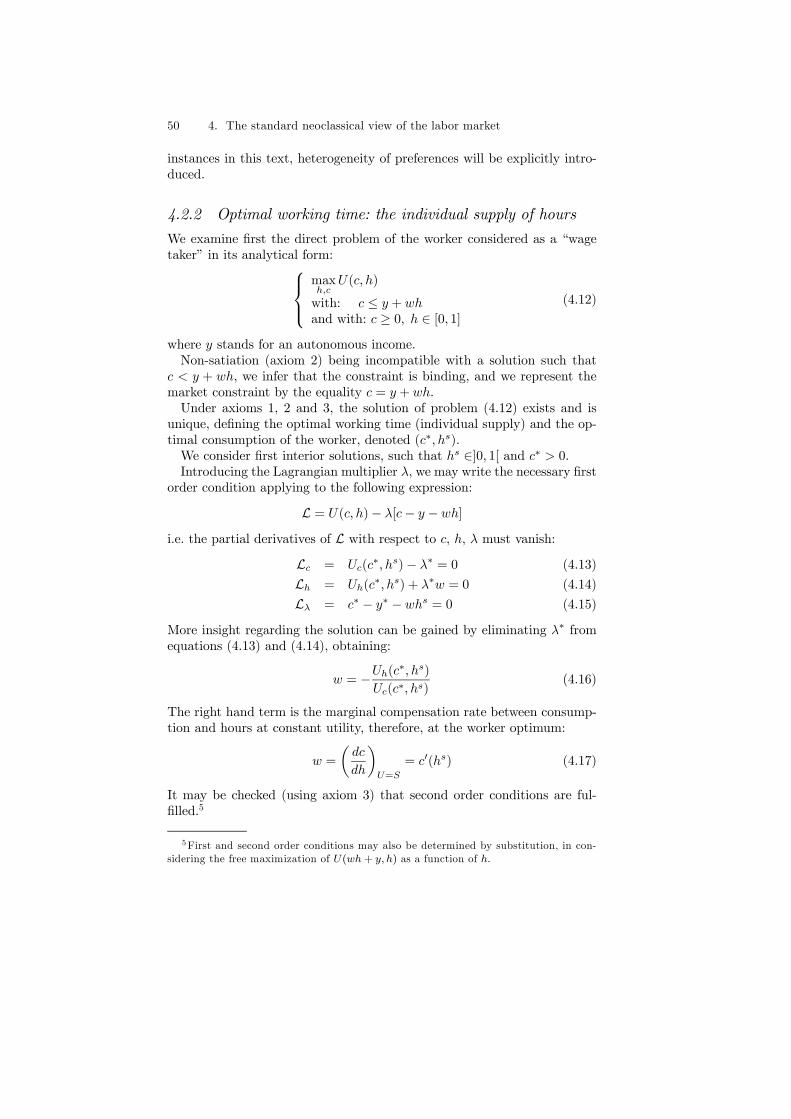
50 4. The standard neoclassical view of the labor market
instances in this text, heterogeneity of preferences will be explicitly intro-duced.
4.2.2 Optimal working time: the individual supply of hours
We examine first the direct problem of the worker considered as a “wagetaker” in its analytical form:⎧⎪⎨⎪⎩
maxh,c
U(c, h)
with: c ≤ y + whand with: c ≥ 0, h ∈ [0, 1]
(4.12)
where y stands for an autonomous income.Non-satiation (axiom 2) being incompatible with a solution such that
c < y + wh, we infer that the constraint is binding, and we represent themarket constraint by the equality c = y + wh.Under axioms 1, 2 and 3, the solution of problem (4.12) exists and is
unique, defining the optimal working time (individual supply) and the op-timal consumption of the worker, denoted (c∗, hs).We consider first interior solutions, such that hs ∈]0, 1[ and c∗ > 0.Introducing the Lagrangian multiplier λ, we may write the necessary first
order condition applying to the following expression:
L = U(c, h)− λ[c− y − wh]
i.e. the partial derivatives of L with respect to c, h, λ must vanish:
Lc = Uc(c∗, hs)− λ∗ = 0 (4.13)
Lh = Uh(c∗, hs) + λ∗w = 0 (4.14)
Lλ = c∗ − y∗ − whs = 0 (4.15)
More insight regarding the solution can be gained by eliminating λ∗ fromequations (4.13) and (4.14), obtaining:
w = −Uh(c∗, hs)
Uc(c∗, hs)(4.16)
The right hand term is the marginal compensation rate between consump-tion and hours at constant utility, therefore, at the worker optimum:
w =
µdc
dh
¶U=S
= c0(hs) (4.17)
It may be checked (using axiom 3) that second order conditions are ful-filled.5
5First and second order conditions may also be determined by substitution, in con-sidering the free maximization of U(wh+ y, h) as a function of h.
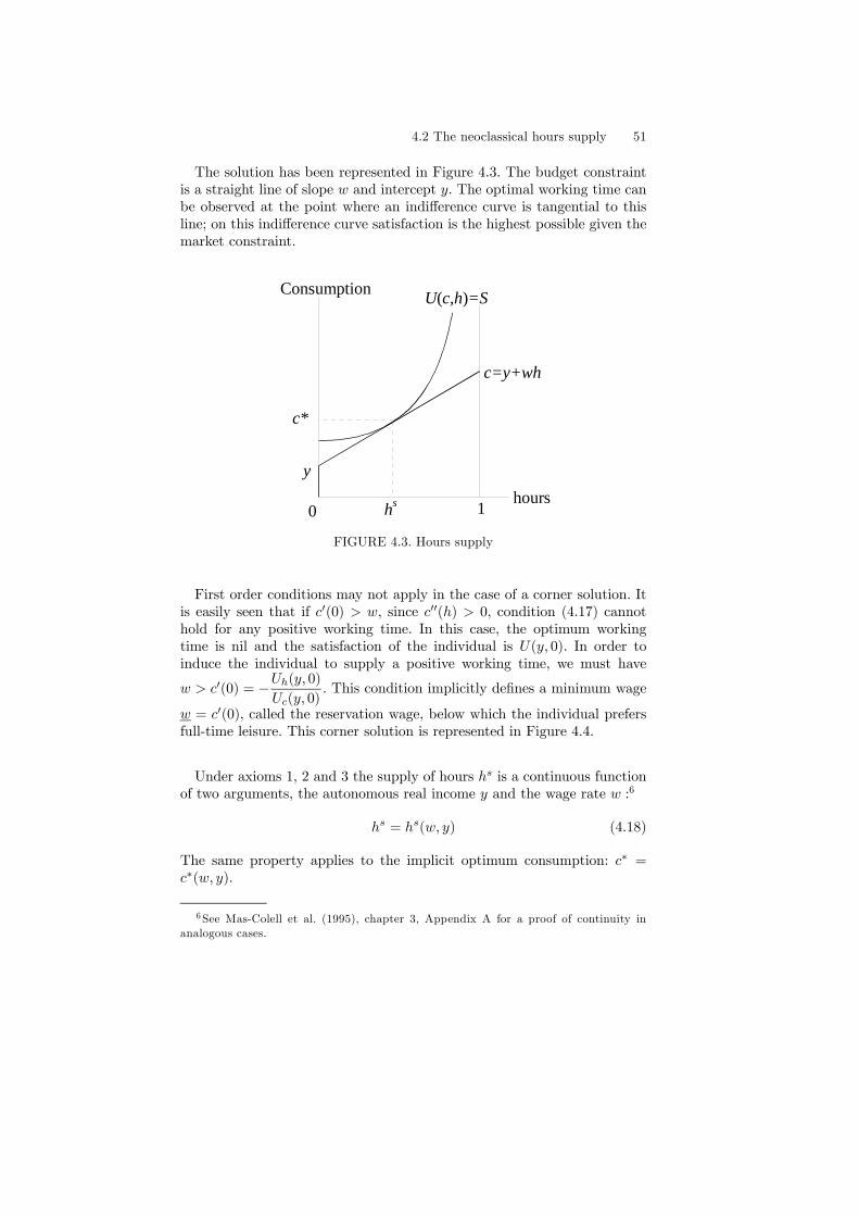
4.2 The neoclassical hours supply 51
The solution has been represented in Figure 4.3. The budget constraintis a straight line of slope w and intercept y. The optimal working time canbe observed at the point where an indifference curve is tangential to thisline; on this indifference curve satisfaction is the highest possible given themarket constraint.
0hours1
Consumption U(c,h)=S
y
c=y+wh
c*
hs
FIGURE 4.3. Hours supply
First order conditions may not apply in the case of a corner solution. Itis easily seen that if c0(0) > w, since c00(h) > 0, condition (4.17) cannothold for any positive working time. In this case, the optimum workingtime is nil and the satisfaction of the individual is U(y, 0). In order toinduce the individual to supply a positive working time, we must have
w > c0(0) = −Uh(y, 0)Uc(y, 0)
. This condition implicitly defines a minimum wage
w = c0(0), called the reservation wage, below which the individual prefersfull-time leisure. This corner solution is represented in Figure 4.4.
Under axioms 1, 2 and 3 the supply of hours hs is a continuous functionof two arguments, the autonomous real income y and the wage rate w :6
hs = hs(w, y) (4.18)
The same property applies to the implicit optimum consumption: c∗ =c∗(w, y).
6 See Mas-Colell et al. (1995), chapter 3, Appendix A for a proof of continuity inanalogous cases.

52 4. The standard neoclassical view of the labor market
0hours1
Consumption
y
c = y + wh_
S
FIGURE 4.4. The reservation wage
The supply curve is usually understood as the partial relationship hs(w)between the working hours offered by the individual and the wage rate. Agreat deal of attention has been given, in particular, to the sensitivity ofthe labor supply with respect to the wage rate, ∂hs(w, y)/∂w.
4.2.3 The compensated working time supply
In order to analyze in depth the shape of the labor supply curve, we sug-gest introducing first the auxiliary concept of “compensated working timesupply”.Let us consider a new problem: determine in the (Oc,Oh) space the point
(c, h) minimizing the autonomous income y necessary to enable the workerto attain utility level S, when the wage rate is w.In analytical form, this problem can be written:⎧⎨⎩ min {y}
with: y = c− whand with: U(c, h) ≥ S
(4.19)
The utility constraint is clearly binding and first order conditions must befulfilled in the following Lagrangian form:
L =c− wh− σ [U(c, h)− S]
Lc = 1− σUc(c, h) = 0 (4.20)
Lh = −w − σUh(c, h) = 0 (4.21)
Lσ = U(c, h)− S = 0 (4.22)

4.2 The neoclassical hours supply 53
Elimination of σ from the first two equations shows that w = −Uh(c, h)Uc(c, h)
,
and using equation (4.10):
w = c0(h) (4.23)
As a consequence of our assumptions, the compensated labor supply func-tion is a continuous function of its arguments:
h = h(w,S)
Differentiating equation (4.23) gives the sign rule:
∂h
∂w=
1
c00(h)> 0 (4.24)
The objective function takes its minimum value y = c−wh; from the conti-nuity of the compensated equilibrium and from its definition, the objectivefunction is itself continuous in S and w and is denoted y = y(w,S).
Proposition 4 It can be shown that ∂y/∂w = −h.Proof. Since y = c− wh :
∂y
∂w=
∂c
∂w− h− w
∂h
∂w(4.25)
Differentiating (4.22) with respect to w yields: Uc∂c
∂w+ Uh
∂h
∂w= 0; hence
from (4.20) and (4.21),1
σ
"∂c
∂w− w
∂h
∂w
#= 0 and finally, from (4.25):
∂y
∂w= −h (4.26)
4.2.4 The response of the individual labor supply to the wagerate
We are now able to analyze the effect of a change of the wage rate on theoptimum working time, using the following identity:7
h(w,S) = hs [w, y(w,S)] (4.27)
7For an illustration of dual methods in the context of standard consumption theory,see Mas-Colell et al. (1995), chapter 3.

54 4. The standard neoclassical view of the labor market
This basic identity means that the point (c, h) may be given two possibleinterpretations: it is the solution of (4.19) and also the solution of (4.12) ify = y(w,S).Differentiating both members with respect to w, we obtain:
∂h
∂w=
∂hs
∂w+
∂hs
∂y
∂y
∂w
and using equation (4.26):
∂hs
∂w=
∂h
∂w+ h
∂hs
∂y(4.28)
If the wage rate increases, the worker’s response may be considered as thesum of two components.The first component is a pure substitution effect: given that one hour of
work is better paid, the compensated individual tends to substitute leisurewith consumption and would like to work more: ∂h/∂w > 0.The second is an autonomous income effect. The sign of this income effect
is left undetermined by the accepted axioms on preferences. If leisure is an“inferior” commodity, increased income prompts workers to supply moreworking hours, ∂hs/∂y > 0; in this case, there is no ambiguity about thesign of the individual labor supply response, as both effects go in the samedirection, ∂hs/∂w > 0.However, in the opposite case in which leisure is a “normal” commodity,
in other words, if people tend to increase their demand for leisure whentheir autonomous income increases, ∂hs/∂y < 0. In this case, the net effectof the wage increase depends on the magnitude of the two components,∂hs/∂w ≶ 0.Figure 4.5 depicts a situation in which leisure is a normal commodity,
and in which the substitution effect prevails.
When the wage rate increases from w1 to w2, the substitution effectwould increase working time to h3, but the income effect tends to offsetthis first term, final working time being h2; in this case h2 is still largerthan h1.In the presence of a positive autonomous income (y > 0), equation (4.28)
lends itself to an analysis in elasticity terms: multiplying both members ofequation (4.28) by w/h, this takes the form:
ηhs
w = ηhw + θηhs
y (4.29)
where θ = wh/y represents the ratio of labor earned income over au-tonomous income, ηh
s
w stands for the uncompensated wage elasticity ofhours of work, ηhw is the income compensated wage elasticity (income is

4.2 The neoclassical hours supply 55
0 hours1
Consumption
y
c = y + w1h
h1
c = y + w2h
c = y + w2h
h3h2
^
y
FIGURE 4.5. Income and substitution effects
adjusted to hold utility constant), while θηhy is the so-called “total incomeelasticity” (Pencavel 1986).If there is no autonomous income, y = 0, θ = +∞, ηh
s
y = 0 but by
definition, θηhs
y = w∂hs
∂y.
4.2.5 Empirical estimates of labor supply functions
As mentioned in Chapter 1, the first forms of this analysis were suggestedby Lionel Robbins (1930) who argued quite convincingly that only empiricalanalysis could reveal the actual form of the relationship between wages andthe working hours supply; since an early attempt to estimate hours supplyfunctions by Douglas (1934), an impressive number of studies have beendevoted to this issue. According to Pencavel (1986, p.3) “labor supply hasbecome the most active area of all labor economics research”.Most empirical estimates use cross-sectional data to reveal the supply
behavior in the short run. These studies analyze workers’ participation orannual hours of work as they are affected by wage rates (w in our notation)or unearned income (y). As emphasized by Ehrenberg and Smith (1994),the most reliable studies are those which focus on hours supply of men,since the supply decision of women is highly sensitive to child-rearing andhousehold work arrangements for which data are sketchy at best.Pencavel (1986) quotes fourteen studies on the hours response of Amer-
ican men carried out in the seventies and eighties. The central tendency ofestimates of the uncompensated wage elasticity of hours of work lies be-

56 4. The standard neoclassical view of the labor market
tween [−0.17, 0.08], and a simple average of all estimates (except a positiveoutlier) is ηh
s
w = −0.12. According to the same author, from these studies itmay be reasonably inferred that ηhw = 0.11 and the total income elasticityis θηhy = −0.23. Apart from two papers, all the other studies found thatthe income effect is negative, thus leisure appears to be a normal good. Healso surveys several studies on British men, and finds support for a similarconclusion, in favor of a seemingly backward bending supply curve.As far as women are concerned, supplied working time seems to exhibit
positive response to wage increases. Killingsworth and Heckman (1986) andBlundell (1993) survey several studies carried out in the eighties and earlynineties, most of them reporting positive uncompensated elasticities andnegative income elasticities. For instance, the uncompensated wage elastic-ity of hours of work reported in the eight studies surveyed by Blundell liesin the interval [0.10, 0.71], with an outlier of 1.44. Of course, the behav-ior of women appears to be highly sensitive to marital status, the numberof children and the age of children. As a rather general feature, all thesecross-sectional analyses for men and women conclude that both income andsubstitution effects are small.Long run supply behavior is difficult to grasp, insofar as many factors
are unstable. As mentioned in Chapter 2, in the last 200 years, hours ofwork have declined throughout the Western world while wages and GDPper inhabitant have risen steadily. If one reasonably assumes that technicalprogress is responsible for an upward shift of the demand for labor services,in the light of this chapter, the observed tendency would suggest that thehour supply curve must be backward bending. However, in the eighties thedownward trend in working hours tended to stabilize and even to reversein some countries. The elementary neoclassical model could be made con-sistent with this observation if the supply becomes at least locally morerigid. Costa (1998) brings out some evidence in favor of this view.
All workers Hourly workers1890s −0.304 −0.5361973 −0.087 −0.0231991 −0.017 +0.104
TABLE 4.1. Elasticity of daily hours worked with respect to the hourly wage.American men aged 25-64. Source: Costa (1998)
4.2.6 Surplus from work
As mentioned before, when the wage rate is higher than the lower reser-vation limit, workers supply a positive amount of time, hs(w) > 0; this

4.2 The neoclassical hours supply 57
optimum working time enables the individual to increase his utility fromthe value S0 = U(y, 0) to S∗ = U(y + whs, hs).The surplus from work is defined by the autonomous income increase v
which would compensate the individual for being prevented from workingat all. It is implicitly defined by:
U(y + v, 0) = S∗
This compensation is represented in Figure 4.6.
0 hours1
Consumption
hs
yy+v
S0S*
FIGURE 4.6. Surplus from work
A general expression for the compensation of wage variations may be ob-tained from properties of the objective function in the compensated prob-lem (4.19). For instance, if the wage rate decreases from the initial valuew1 to the final value w2, by definition of the function y(w,S), the necessarycompensation is γ(w1, w2) = y(w2, S
∗1)− y(w1, S∗1) where S∗1 is the satisfac-
tion level reached in the initial equilibrium: S∗1 = U [y + w1hs(w1), h
s(w1)].
Since ∂y/∂w = −h, this may be written γ(w1, w2) = −w2Zw1
h(w,S∗1)dw. It
can be represented by the grey shaded area at the left of the compensatedsupply curve and between the two horizontal lines of ordinates w2 and w1(Figure 4.7), where it may be seen that h(w,S∗) = 0 for small values of w.
In this perspective, surplus from work may be viewed as the compensa-tion for a wage variation going from an initial value w1 to zero:
v = γ(w1, 0) =
w1Zw=0
h(w,S∗1)dw

58 4. The standard neoclassical view of the labor market
0 hours
wage rate
w1
w2
h (w)sh(w)^
FIGURE 4.7. Compensation of a wage rate decrease
4.3 Comments on the elementary neoclassicalmodel of hours supply
4.3.1 The composite good: a caveat about relative prices
We have used in the above analysis the familiar notion of the real wagerate. In using the compact notation S = U(c, h) we consider either thatonly one good exists in the economy or that c stands for the consumptionof a composite commodity. In the latter case, a utility function U(c, h)may be defined in the following way. Recording the consumption of them goods by (x1...xi...xm), we consider first a neoclassical utility functionV (x1...xi...xm, h) (with Vh < 0) representing constant preferences and de-note (x∗1...x
∗i ...x
∗m) the vector of consumption, solution of the problem:⎧⎪⎨⎪⎩
maxx1...xi...xm
V (x1...xi...xm, h)
with:mXi=1
pixi ≤ c(4.30)
where c and h are considered predetermined and where pi represents themoney price of the ith good. From standard demand theory, (x∗1...x
∗i ...x
∗m)
is uniquely determined and is a continuous function of c, h and all pricespi. It is possible to define U(c, h) by U(c, h) = V (x∗1...x
∗i ...x
∗m, h); this new
function is an “indirect utility function”, c standing for a money flow ofincome available for consumption. This function is well defined for a givenprice structure and satisfies axioms 1, 2 and 3.8
8Proof of this statement is a technical exercice omitted here.

4.3 Comments on the elementary neoclassical model of hours supply 59
In what sense can we say that a constant wage rate implies a constantlabor supply when c stands for a composite commodity ?To illustrate the problem in intuitive terms, consider the following case.
A worker is so fond of golf that in an initial situation, he spends as muchmoney playing his favorite sport as purchasing food. In a first assumption,we imagine that the price of food is increased by 20%, other prices beingconstant. His nominal wage rate is adjusted in order to make the consump-tion and leisure-time bundle of the initial reference state exactly possible.In a second assumption, the hourly cost of golf is increased by 20%, otherprices being constant. Once again, his nominal wage rate is adjusted inorder to make the consumption and leisure-time bundle of the initial ref-erence state exactly possible. We can say that the worker is compensatedin both cases, and that the real wage rate has been in some sense keptconstant. Can we predict that this worker’s labor supply is affected in thesame way?When the price of food increases, the compensated worker tends to reduce
somewhat his consumption because of the substitution effect, but eatingless or eating lower quality food does not impinge so directly on the durationof meals and on the demand for leisure. When the price of golf increases,the compensated worker with neoclassical preferences is going to reducetime spent on golf courses and this could very well induce him to supplymore working hours.In order to examine the effects of changes in prices, the worker’s problem
may be rewritten in terms of the direct utility function:⎧⎪⎨⎪⎩max
x1...xi...xm,hV (x1...xi...xm, h)
with:mXi=1
pixi =Wh+ Y(4.31)
In problem (4.31), the wage rate W and the income Y are in money terms.The first order conditions applying to the Lagrangian form associated tothis problem are:
Vi − λpi = 0, ∀i = (1, ...,m)Vh + λW = 0mXi=1
pix∗i =Whs + Y
(4.32)
The resulting labor supply function is of the form:
hs = hs(p1...pi...pm,W, Y ) (4.33)
This function clearly verifies the following homogeneity property:
∀µ > 0, hs(µp1...µpi...µpm, µW, µY ) = hs(p1...pi...pm,W, Y ) (4.34)
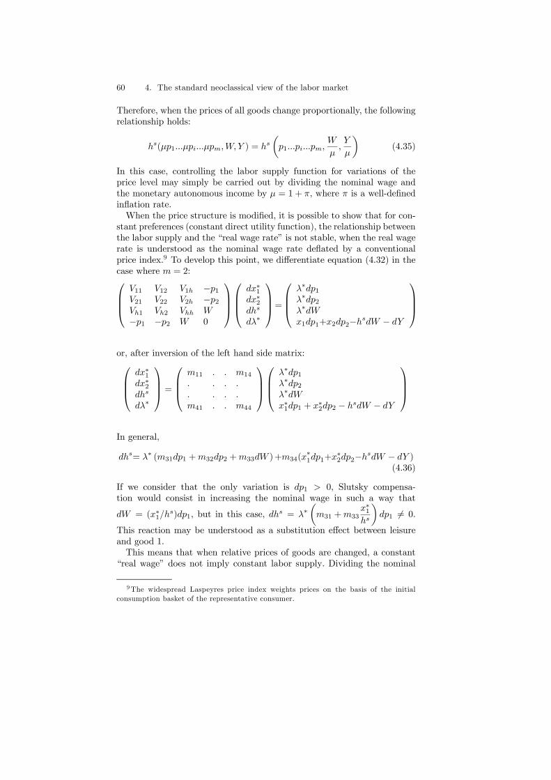
60 4. The standard neoclassical view of the labor market
Therefore, when the prices of all goods change proportionally, the followingrelationship holds:
hs(µp1...µpi...µpm,W, Y ) = hsµp1...pi...pm,
W
µ,Y
µ
¶(4.35)
In this case, controlling the labor supply function for variations of theprice level may simply be carried out by dividing the nominal wage andthe monetary autonomous income by µ = 1 + π, where π is a well-definedinflation rate.When the price structure is modified, it is possible to show that for con-
stant preferences (constant direct utility function), the relationship betweenthe labor supply and the “real wage rate” is not stable, when the real wagerate is understood as the nominal wage rate deflated by a conventionalprice index.9 To develop this point, we differentiate equation (4.32) in thecase where m = 2:⎛⎜⎜⎝
V11 V12 V1h −p1V21 V22 V2h −p2Vh1 Vh2 Vhh W−p1 −p2 W 0
⎞⎟⎟⎠⎛⎜⎜⎝
dx∗1dx∗2dhs
dλ∗
⎞⎟⎟⎠=⎛⎜⎜⎝
λ∗dp1λ∗dp2λ∗dWx1dp1+x2dp2−hsdW − dY
⎞⎟⎟⎠
or, after inversion of the left hand side matrix:⎛⎜⎜⎝dx∗1dx∗2dhs
dλ∗
⎞⎟⎟⎠ =
⎛⎜⎜⎝m11 . . m14
. . . .
. . . .m41 . . m44
⎞⎟⎟⎠⎛⎜⎜⎝
λ∗dp1λ∗dp2λ∗dWx∗1dp1 + x∗2dp2 − hsdW − dY
⎞⎟⎟⎠
In general,
dhs= λ∗ (m31dp1 +m32dp2 +m33dW )+m34(x∗1dp1+x
∗2dp2−hsdW − dY )
(4.36)
If we consider that the only variation is dp1 > 0, Slutsky compensa-tion would consist in increasing the nominal wage in such a way that
dW = (x∗1/hs)dp1, but in this case, dhs = λ∗
µm31 +m33
x∗1hs
¶dp1 6= 0.
This reaction may be understood as a substitution effect between leisureand good 1.This means that when relative prices of goods are changed, a constant
“real wage” does not imply constant labor supply. Dividing the nominal
9The widespread Laspeyres price index weights prices on the basis of the initialconsumption basket of the representative consumer.
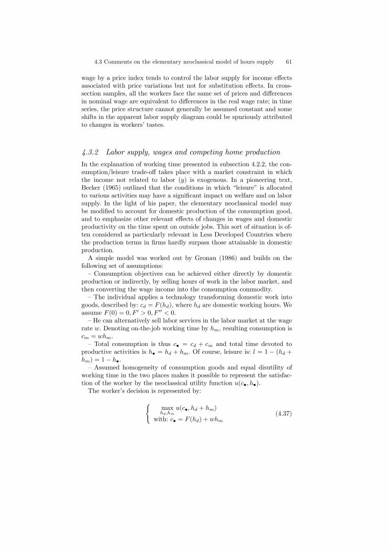
4.3 Comments on the elementary neoclassical model of hours supply 61
wage by a price index tends to control the labor supply for income effectsassociated with price variations but not for substitution effects. In cross-section samples, all the workers face the same set of prices and differencesin nominal wage are equivalent to differences in the real wage rate; in timeseries, the price structure cannot generally be assumed constant and someshifts in the apparent labor supply diagram could be spuriously attributedto changes in workers’ tastes.
4.3.2 Labor supply, wages and competing home production
In the explanation of working time presented in subsection 4.2.2, the con-sumption/leisure trade-off takes place with a market constraint in whichthe income not related to labor (y) is exogenous. In a pioneering text,Becker (1965) outlined that the conditions in which “leisure” is allocatedto various activities may have a significant impact on welfare and on laborsupply. In the light of his paper, the elementary neoclassical model maybe modified to account for domestic production of the consumption good,and to emphasize other relevant effects of changes in wages and domesticproductivity on the time spent on outside jobs. This sort of situation is of-ten considered as particularly relevant in Less Developed Countries wherethe production terms in firms hardly surpass those attainable in domesticproduction.A simple model was worked out by Gronau (1986) and builds on the
following set of assumptions:— Consumption objectives can be achieved either directly by domestic
production or indirectly, by selling hours of work in the labor market, andthen converting the wage income into the consumption commodity.— The individual applies a technology transforming domestic work into
goods, described by: cd = F (hd), where hd are domestic working hours. Weassume F (0) = 0, F 0 > 0, F 00 < 0.— He can alternatively sell labor services in the labor market at the wage
rate w. Denoting on-the-job working time by hm, resulting consumption iscm = whm.— Total consumption is thus c• = cd + cm and total time devoted to
productive activities is h• = hd + hm. Of course, leisure is: l = 1 − (hd +hm) = 1− h•.— Assumed homogeneity of consumption goods and equal disutility of
working time in the two places makes it possible to represent the satisfac-tion of the worker by the neoclassical utility function u(c•, h•).The worker’s decision is represented by:(
maxhd,hm
u(c•, hd + hm)
with: c• = F (hd) + whm(4.37)

62 4. The standard neoclassical view of the labor market
The corresponding Lagrangian form is:
L = u(c•, hd + hm)− λ[c• − F (hd)− whm] (4.38)
entailing first order conditions:
uc = λ (4.39)
uh = λF 0(hd) (4.40)
uh = λw (4.41)
Thus from equation (4.40) and equation (4.41) we have F 0(hd) = w which
defines hsd, and from (4.39) and (4.41), MRS =
µdc
dh
¶U=S
= −UhUc
= w
which defines total hours supply hs•. Then hsm = hs• − hsd.The solution is depicted in Figure 4.8:
0hours
1
Consumption
c = cd + whm
cd
c cd = F(hd)
y
hds hs.
FIGURE 4.8. Optimal working time: at home and on-the-job
In order to analyze the response of the market supply of labor hsm towage rate fluctuations, it is possible to consider the two logically consecu-tive stages of the worker’s decision. The first decision consists in working athome for a time hsd, solely determined by F
0(hd) = w. This first decision de-termines the market line and its intercept on the vertical axis noted y. In asecond stage, the worker’s choice may be interpreted as a standard workingtime decision in which the “autonomous” income y becomes a function ofthe wage rate w denoted y(w).With the help of Figure 4.8 it can be checked
that y(w) = F (hsd)−whsd and thereforedy
dw= [F 0(hsd)− w]
dhsddw−hsd = −hsd.

4.3 Comments on the elementary neoclassical model of hours supply 63
Considering the total working time as a function of w, we can write thefollowing identity:
hs•(w) = hs [w, y(w)] (4.42)
Thereforedhs•(w)
dw=
∂hs
∂w+
∂hs
∂y
dy
dw=
∂hs
∂w− hsd
∂hs
∂y. The term
∂hs
∂witself
can be decomposed to substitution and income effects according to equation
(4.28):∂hs
∂w=
∂h
∂w+ hs•
∂hs
∂y. We then have:
dhs•dw
=∂h
∂w+ (hs• − hsd)
∂hs
∂y=
∂h
∂w+ hsm
∂hs
∂y
Also, F 0(hsd) = w impliesdhsddw
=1
F 00(hd).
Since hsm = hs• − hsd, we finally obtain:
dhsmdw
=dhs•dw− dhsd
dw=
∂h
∂w+ hsm
∂hs
∂y− 1
F 00(hsd)(4.43)
The effect of an increased wage rate on the supply of market hours by work-ers having their own productive abilities is decomposed into three terms.Only the income effect, restricted to hours sold on the market may be neg-ative. The order of magnitude of the third term can be overwhelming if thetechnology is close to linearity, F 00(hd) taking small values. The responseof labor supply for this type of worker may therefore be very different fromthe standard prediction.
4.3.3 Reservation wage and lump-sum cost of working: aquantum
The standard labor supply theory implies strong continuity properties; inparticular, when the wage rate decreases toward its reservation value asdefined in subsection 4.2.2, the supplied working time continuously dimin-ishes and approaches zero. Very short working durations are however rarelyobserved, a fact which can be interpreted in labor supply terms if we in-troduce more details into the worker’s feasible set description. We considerthat the worker incurs a fixed cost z if working. This lump sum may beinterpreted as the cost of having to commute to the workplace and arrivewith a suitable appearance, but it may more significantly include the lossof support or subsidy granted to the unemployed. In this case the laborsupply is hs(w, y− z) if the resulting satisfaction equals or exceeds the sat-isfaction level recorded when not working at all, but saving the fixed cost.This more encompassing notion of reservation wage ew is therefore defined

64 4. The standard neoclassical view of the labor market
as the solution of the following equation:
U [y − z + whs(w, y − z), hs(w, y − z)] = U(y, 0)
Worker’s behavior in the presence of lump costs can be represented by thesupply function:
hs =
½hs(w, y − z), for w ≥ ew
0, for w < ewWhen the wage rate decreases towards the reservation limit, labor supplytends to an indivisible quantum of working time, denoted eh. Figure 4.9illustrates the determination of ew and eh.
0hours1
Consumption
y
h~
y-z
wh~
c(h)
c~
FIGURE 4.9. Reservation wage with “commuting” costs
We show how the reservation wage rate in the case where unemploymentbenefits are lost by the incumbent workers modifies the representation ofoutside equilibrium in the labor market. According to equation (4.7), thefirm demand for workers takes the form:
n∗(w) =L∗(w)
hs(w)
The demand for workers does not exist where w < w since in this casehs(w) = 0. The number n∗(w) represents the maximum amount of workerswillingly hired by the representative firm.The supply of workers per firm (each providing hs(w)) is:
ns =
½N/f, if w ≥ w0, if w < w

4.4 Conclusion 65
workers
wage rate
0
N/f
w
n*
~
n*(w)~ ns
E
FIGURE 4.10. Involuntary unemployment
that is, the participation rate becomes nil for wages inferior to the reserva-tion wage rate.If the demand for workers is weak, the special situation depicted in Fig-
ure 4.10 may arise: n∗(w) < N/f. Workers are indifferent between holdinga job or not; those who do not have one (ns − n∗(w)) can either be calledinvoluntary unemployed, insofar as they would take an available job atthe going wage, or voluntary unemployed, since their situation is a con-sequence of their preferences and since they incur no welfare loss fromunemployment.10
It may be checked that ew = c0(eh) and convex indifference curves implythat ew and eh are both increasing in z. In the Appendix to this chapter,the reservation wage and the corresponding quantum of working time areexplicitly calculated as functions of the fixed cost z for a simple theoreticalutility function.
4.4 Conclusion
In this chapter, emphasis was placed on the analysis of the labor supply,which dominated the early period of neoclassical economics. We show howconsiderations on consumption/leisure preferences themselves may explainthe variety of durations of work, for a non-differentiated flow of labor ser-vices provided to firms. One of the main shortcomings of this elementaryneoclassical view is its incapacity to account for obvious worker rationing
10See De Vroey (1998) for an analysis of the two terms in historical perspective.

66 4. The standard neoclassical view of the labor market
and systematic conflicts over working hours. These difficulties come fromthe obvious oversimplification of the demand side. In the late sixties, someauthors begin to pay more attention to the composition of the flow of laborservices. The next chapter proposes a brief description of these advancesand develops an original description of the productive process, introducingthe concept of “output density function”.
4.5 Appendix: Examples of theoretical utilityfunctions
We suggest examining basic utility functions able to convey the three ax-ioms concerning preferences adopted in this chapter and to illustrate simplysome of the proposed concepts. The time unit is the day so h ∈ ]0, 1[ .• U = c(1− h)Axioms 1, 2 and 3 hold; a fixed level of satisfaction S defines a compen-
sating function (or an indifference curve) c(h) = S/(1− h).
The first derivative c0(h) =
µdc
dh
¶U=S
= S(1 − h)−2 and the second
derivative c00(h) = 2S(1− h)−3 are both defined and positive for h ∈]0, 1[.The corresponding hours supply function is hs(w, y) = (w−y)/2w, where
y is an autonomous income.For w ≥ S,the compensated labor supply function is h(w,S) = 1−
pS/w.
In the absence of fixed costs entailed by working, the reservation wageis w = y. If the fact of working implies the loss of z consumption units(foregone unemployment benefits), a new value of the reservation wage canbe computed. This value is the solution of: U [y − z + whs(w), hs(w)] =U(y, 0); applying the assumed utility function, it may be shown that therelevant solution of this equation is ew = z+y+2
√zy, an increasing function
of z; the quantum of labor supplied for this value of the wage rate is eh =z +√zy
z + y + 2√zy
. It may be checked that z = 0 ⇒ ew = y and eh = 0.• U = (c− c0)
α(1− h)1−α, α ∈ ]0, 1[This utility function introduces a term c0 which may be interpreted as a
subsistence consumption; preferences are not defined for c < c0.A given satisfaction level S defines an indifference curve c(h) = c0 +
S1α (1− h)
α−1α .
The slope of the indifference curve is therefore: c0(h) =µdc
dh
¶U=S
=
S1α
µ1− α
α
¶(1− h)−
1α =
µ1− α
α
¶µc− c01− h
¶> 0 ∀h ∈ ]0, 1[ , the param-
eter α tuning the slope of the indifference curve.

4.5 Appendix: Examples of theoretical utility functions 67
The compensating function is convex c00(h) = S1α
µ1− α
α2
¶(1−h)−
1+αα >
0 ∀h ∈ ]0, 1[ .The hours supply function is hs(w, y) = α+[(c0−y)(1−α)]/w; therefore,
∂hs/∂w is nil if y = c0, negative if y < c0 and positive if y > c0.The reservation wage is w = (y − c0)(1− α)/α, increasing with y.This utility function is able to illustrate the mercantilist view of labor
supply mentioned in Chapter 1. Consider the case where y = 0 (workershave no autonomous income). In this case, hs(w, 0) = α+c0(1−α)/w imply-ing lim
α→0{hs(w, 0)} = c0/w. This limit depicts a situation in which no finite
increase in consumption would be able to compensate an increased workingtime when the subsistence requirement is satisfied. It involves ηh
s
w = −1.
• Quasi-linear utility functions
It is often convenient to use quasi-linear utility functions, i.e. functions ofthe form U(c, h) = c−v(h), where v(h) is a convex function such that v(0) =0, v0(h) > 0, v00(h) > 0. Such functions generate convex compensatingfunctions (or indifference curves) defined for any given value of S by c(h) =S + v(h) and therefore c0(h) = v0(h) and c00(h) = v00(h) > 0. The hourssupply function is hs(w) = v0−1(w), with dhs/dw = 1/v00(h) > 0.In a space (Oh,Oc), the satisfaction level related to an indifference curve
has a consumption equivalent visualized by the ordinate c(0) = S. Thesurplus derived fromWalrasian supply in the labor market is also visualizedon the vertical axis. (An application of these functions to working timetheory will be provided in Chapter 7.)

68 4. The standard neoclassical view of the labor market

This is page 69Printer: Opaque this
5Working time, production and costfunctions
5.1 Contemporary demand side contributions toworking time analysis
5.1.1 The critique of the elementary neoclassical approach
The standard textbook analysis of the demand side of the labor marketdraws exclusively on standard production functions, in which the flow oflabor input is entirely defined as the product of the number of employedpeople and the number of hours worked per day, or other implicit timeunit. As seen in Chapter 4, with such production functions, and assumingstandard labor cost functions, the wage-taking firm is totally indifferent tothe composition of the labor input. Competition can therefore bring aboutthe optimal working day from the worker’s point of view, corresponding tothe notional labor supply.Production and cost functions are in fact symbolic and highly simplified
representations of the economically relevant aspects of complex productionprocesses. They are generally conceived as parsimonious tools, able to inte-grate the most basic properties of firm behavior into broader descriptionsof the economic system. As building blocks of involved models, their owncomplexity must be kept at sufficiently low levels.More formally, production functions — in the standard form — explain
which flow of output y can be obtained by applying a stock of capitalK, and a flow of labor services L. This relationship is represented by a

70 5. Working time, production and cost functions
concave, twice differentiable function F (K,L). The neoclassical standardform implies, in particular, the following assumptions:
1. The stock of capital is generally considered to be composed of Khomogeneous equipment units.
2. The flow of labor services is (most often implicitly) supposed to beof the form L = nh, where n is the number of homogeneous workersand h is the number of homogeneous hours.
3. The total cost incurred by the producer is explained by the samevariables, and the currently used functions are of the form C(K,L) =wL+ (δ+ r)K. Its first term is the wage bill, where w stands for thehourly real wage rate. The second term is the rental cost of capitalincluding an exponential depreciation component represented by δKand a financial cost rK, where r is the prevailing real interest rate.By a suitable choice of units, the price of the capital unit is equal toone.
Under these assumptions, the profit function is also concave: π(K,L) =F (K,L)− wL− (δ + r)K.From standard microeconomic analysis, we know that first order condi-
tions are therefore sufficient to characterize a profit global maximizationinput mix. The corresponding point (K∗, L∗) = argmax {π(K,L)} is theunique solution, and is such that K∗ = K∗(w, δ+ r) and L∗ = L∗(w, δ+ r)are continuous functions of their arguments. Since hours supplied by out-siders or by insiders are perfect substitutes in the productive process, andsince labor costs are wL, isoquants and isocosts in space (Oh,On) coa-lesce in the hyperbola representing the equation L∗ = nh. In this case,as explained in detail in Chapter 4, firms are strictly neutral in terms ofworking time, and indetermination on (n, h) can be lifted by the workers’preferences.Historical evidence has revealed, however, the existence of persistent con-
flicts between employees and firms over working time (Chapter 2). Twotypes of disequilibrium especially should be considered: overwork, i.e. thesituation where the duration of work determined by the firm exceeds theWalrasian labor supply and insider underemployment, the opposite ra-tioning in which the worker is constrained to more leisure than demandedfor the current wage rate. Explaining the actual working time and imper-fect equilibrium in a decentralized economy has thus required improveddescriptions of labor costs or production processes.As far as costs structures are concerned, most authors apply the two-part
form pioneered by Rosen (1968):
C(w,n, h) = n(wh+ θ) (5.1)
5.1 Contemporary demand side contributions to working time analysis 71
where the product of the real wage rate w and individual hours h representsthe total wage bill (or wage compensation), and θ stands for the “fixed costsof labor”.The wage rate may itself be considered as predetermined, or depending
on other variables, including in particular the duration of work.Fixed costs of labor are expenses depending only on the number of work-
ers and independent of the working time; in some sectors such costs may bequite substantial.1 An exhaustive list of these costs is impossible to drawup, but we can mention: costs incurred in providing the workers with in-dividual equipment and job environment (personal computer, office room,lunch facilities, etc.), management of the personnel files, etc. Firms oftenhave to provide workers with some form of specific training; they conse-quently incur in the steady state various costs proportionate to the staffand to the staff turnover, as well as a financial cost induced by investmentsunk in human capital.It is worth noticing that the distribution of labor costs in fixed and
variable forms is also affected by government interference and regulation.In most OECD countries, social charges collected from employers for fi-nancing the social welfare and unemployment compensation schemes areindividually limited by a ceiling. For those workers with wages below thisceiling, social charges are still proportional to the wage income, thereforebehaving like variable costs; for workers with wages above the ceiling, thecontribution appears as a lump-sum tax, thus behaving like a fixed cost.In a thorough analysis of non-wage costs, Hart (1984) published quan-
titative estimations of these fixed labor costs in the UK and the US. In1981, the ratio of variable to total (variable plus fixed) costs was around0.89 if payments for days not worked are excluded, or 0.80 if payments fornon-worked days are included.In relation to the productive process, it must be kept in mind that some
early authors, before and throughout the neoclassical period, have provedquite aware of its complex underlying structure and their points of viewwere coined in explicit terms:
Two hundred grenadiers pulling ropes for a few hours havebeen able to lift the Luxor obelisk on the Place de la Concorde; afew grenadiers pulling for two hundred hours could not. (PierreJoseph Proudhon, 1840)...if a man continually works beyond a certain point, the
intensity of his work will be reduced to such an extent thatthe gain in longer hours will be more than offset by the loss inhourly output, so that if he had worked less his average outputwould have been greater. (Lionel Robbins, 1929, p.26 )
1See Oi (1962) for an early analysis of the labor input as a quasi-fixed factor.

72 5. Working time, production and cost functions
Increased leisure means increased facilities for rest and recre-ation; rest and recreation improve physical strength and in-crease alertness; these in their turn react upon efficiency... Somemen might turn out more if the hours were longer, some menmore if they were shorter; but if the total output is maximizedat a given length of day, that length is the optimum. (JohnHicks, 1932, p.105)
5.1.2 Basic Generalized Production Functions
Such considerations are at the core of various generalizations of the produc-tion functions which contemporary labor market analysis has worked out.By definition, Generalized Production Functions (g.p.f.) do away with theimplicit assumption of perfect substitution between workers and hours (inlogarithms). In general terms, g.p.f. are functions of the form:
y = ϕ(n, h,K)
where y is the daily flow of output, n is a continuous variable approximatingthe number of hired workers, h is the daily working time per individual andK is the worker’s capital endowment. Different authors have suggested aparticular g.p.f., able in their view to capture the particular features ofthe productive process they want to emphasize.For instance, Hoel (1986) argues that production in the manufacturing
sector should be represented as:
y = hF (n) (5.2)
F ( ) being a concave function. In his interpretation, equipment is not homo-geneous, the firm employing a stock of machines of varying quality and staffis subject to diminishing returns, because successive workers are equippedwith tools of decreasing efficiency. On the other hand, the output is linearin working time, and this function does not express the effect of exertion onproduction. It must be noticed that Hoel’s function is also compatible withanother (non-exclusive) interpretation according to which the concavity ofF ( ) should be attributed to the productivity structure of a heterogeneouslabor force or to labor coordination effects and not to heterogeneous equip-ment.According to Calmfors and Hoel (1989) output depends on hours and
employment according to the function y = F (nh, shK), where the integers stands for the number of shifts and K is the stock of capital. The productsh indicates in fact the number of hours per day for which the equipment isused. In the case of a production function homogeneous of degree one, wehave for instance: F (nh, shK) = (nh)a(shK)1−a, (a < 1), and the obtainedform is also linear in working time:
y = hF (n, sK) (5.3)

5.1 Contemporary demand side contributions to working time analysis 73
Shift work is often present in those activities where the costs of stoppingand starting production are high (for instance, production of nuclear elec-tric power requires permanent monitoring; steel production also requirescontinuous production flow). Protective services (police, firefighters andemergency health care) also require shift work. However, the bulk of con-temporary production does not rely on such an organization. According todata published by the US Bureau of Labor Statistics, in 1997, 82.9% ofthe full-time paid workers in the United States were on regular daytimeschedules. Only 2.9% of them were on rotating shifts and 8.1% did eveningor night shifts. The same pattern was observed in France, where the Na-tional Institute of Statistics (Insee) recorded that, in 1995, only 10.4% ofthe wage earners worked on regular shifts (Boisard and Fermanian, 1999).Hoel and Vale (1986) observed that firms incur an output loss when
recruiting new employees, as a result of time diversion in training the newlyhired in the workplace. Such losses are thus proportional to the firm’sturnover q, and would justify a production function in which only effectiveworking time contributes to explain output:
y = F [(h− tq)n] = F (nh− tqn) (5.4)
In equation (5.4), q is the turnover rate and t represents the necessarytraining time per employee. In such a case, the output elasticity with respectto hours ηyh should be larger than the output elasticity with respect toworkers ηyn, since from equation (5.4) ηyn = (1− tq/h) ηyh and thereforeηyh > ηyn.As already mentioned, in the conventional neoclassical analysis, the stan-
dard definition of labor services is the total number of hours, i.e. L = nh,and, whatever the production function applied to this flow of labor ser-vices, ηyn = ηyh. Rather than using the general form of g.p.f., the improvedfunctions encountered in modern working time analysis are usually basedon a specific concept of labor services to be included as an argument of theproduction function. This concept acknowledges the fact that the contribu-tion of hours and workers to the flow of labor services may justify a moreflexible representation than the simple multiplicative form, i.e. L = L(n, h)with Ln > 0 and Lh > 0.In this new setting, the marginal contribution to labor services of addi-
tional hours obtained from the employment of a new worker or by extendingthe average working time of incumbent workers may significantly differ. Inthis perspective, labor services are often described by the form introducedby Ehrenberg (1971):
L = ng(h) (5.5)
In this multiplicative form, the “effectiveness function” g(h) indicates theindividual contribution of a worker to the flow of labor services. It is gen-erally assumed that g(0) = 0 and g0(h) > 0, additional time generating

74 5. Working time, production and cost functions
additional output. As emphasized by Hart (1987), it is also most oftensupposed that g00(h) > 0 for some h ≤ h0, “warming-up” or other favor-able effects prevailing and increasing the marginal efficiency for durationsinferior to a threshold h0: in this case, successive equal time increments gen-erate increasing increments of labor services. For “long” durations h > h0,the effects of exertion and perhaps boredom prevail and g00(h) < 0, thatis the contribution of successive time units to the flow of labor servicesdiminishes (Figure 5.1).2
The time structure of the two effects (warming-up and exertion) explainsthe variations in average efficiency g(h)/h. In this context, it is possible todefine the number of hours h1 which maximizes average efficiency. Sinceh1 = argmax {g(h)/h}, from the first order condition for an interior solu-tion, i.e. if h1 ∈ ]0, 1[, this maximization implies g(h1) = h1g
0(h1). If theeffectiveness function is such that g00(h) > 0 for h < h0 and g00(h) < 0 forh > h0 it is possible to show that h1 > h0. For h < h1, increasing hoursentail increasing average efficiency, and beyond this threshold, increasinghours decrease average efficiency. In the light of this comment, it must benoticed that exertion may sometimes occur even if average productivityincreases.Figure 5.1 summarizes the relationship between such an efficiency func-
tion g(h), the marginal efficiency g0(h) and average efficiency g(h)/h. It
must be noticed that, from the l’Hôpital rule, limh→0
g(h)
h= lim
h→0g0(h) ≥ 0.
Researchers have suggested different specifications for the effectivenessfunction. For instance, FitzRoy and Hart (1985) and Hart (1987) haveintroduced two positive parameters τ and , considering that g(h) = 0, forh < τ and g(h) = (h− τ) , for h > τ with 0 < < 1. Time τ is interpretedas closing a “set-up” interval. Although this form reflects exertion as soonas h > τ, since in this case g00(h) < 0, average productivity increases during
a first time interval, then diminishes for h >τ
1− > τ .
Other authors introduced constant elasticity functions, like g(h) = hβ,where β < 1 is interpreted as a dominant fatigue effect, and β > 1 as adominant warming-up effect (see Booth and Schiantarelli, 1987; Andersen,1987; FitzRoy, 1993; D’Autume and Cahuc, 1997).It should be noted in general terms that the introduction of the currently
proposed efficiency functions is nothing but a special way of building ag.p.f., defined for instance by ϕ(n, h,K) = F [ng(h),K]. The empiricalmeaning of the labor services as an argument of a production functionis however questionable, since a degree of freedom is introduced in defin-ing jointly the production function and the labor services input. For in-stance the constant output elasticity function y = Kγnαhβ is a simple
2This form has already been advocated by Chapman (1909).

5.1 Contemporary demand side contributions to working time analysis 75
g(h)
g(h)/h
g' (h)
h1h
h0
0
Worker effectiveness
h0
Average and marginalworker effectiveness
h1
h0
working hours
working hours
FIGURE 5.1. Standard effectiveness function
g.p.f., which can be interpreted in different ways. We can define labor ser-vices by L = nhβ/α; in this case the corresponding production function isy = KγLα. Alternatively, labor services may be defined by L = nα/βh, thecorresponding production function being y = KγLβ . The only empiricallydeterminable relationship is therefore the g.p.f. version relating observableoutput y to observable inputs K,n, h. The two suggested interpretationsin terms of labor services are apparently opposed, since in one case, theselabor services are linear in n, in the other case linear in h. They describehowever the same productive process. Labor services as a malleable andmeasurable input are therefore defined in accordance with some conven-tion. For instance, if there exists in the economy a productive process inwhich the labor services are directly considered as productive without any

76 5. Working time, production and cost functions
collateral factors or intermediation, L = ng(h) may be defining efficiencyg(h) from the output obtained in this particular process by n individualsworking h hours. The flow L, used as an argument of a production functionrelated to other activities, may be interpreted in such a case as a form ofopportunity cost of production.It is important to remark that the notion of labor services has been ex-
tensively used by economists who developed “efficiency wage” models ofthe labor market (see for pioneering papers Solow, 1979; Akerlof, 1982;Shapiro and Stiglitz 1984). In their view, worker effort in the workplacewould be an increasing function of the wage rate relative to some referenceincome obtained from alternative activities. This positive relationship be-tween wages and effort has been justified either by better morale under thegift-exchange paradigm, or by the increasing opportunity costs of shirkingwhen effort on the job is private information to the worker. There werea few attempts to combine working time and efficiency wage approachesbased on more sophisticated g.p.f. For instance, in their production func-tion (equation 5.4), Hoel and Vale (1986) considered that the quit rate qis a decreasing function of the wage rate. Also, Schmidt-Sørensen (1991)proposed an effectiveness function where individual labor services dependnot only on hours of work as in standard working time models, but also onrelative wages as in efficiency wage models.
5.1.3 Empirical estimates of constant output elasticityGeneralized Production Functions
On the empirical side, many researchers, following Feldstein (1967), haveestimated constant output elasticity functions in which hours and employ-ment are separately dealt with. The suggested basic functional form is:
y = F (K,n, h) = AKηKnηnhηh (5.6)
Table 5.1 recapitulates the main results (we only report the most significantvalues of the quoted studies).
ηK ηn ηh DataFeldstein (1967) 0.25 0.76 1.90 UK cross-section, 1960
Craine (1973) 0.12 0.68 1.89US manufacturingpanel 1949-1967
Leslie and Wise (1980) 0.32 0.64 0.64 UK panel, 1948-1968
Åberg (1987) 0.25 0.75 0.71Swedish panel1963-1982
Hart and McGregor (1988) 0.60 0.45 0.99W. German panel1968-1978
TABLE 5.1. Estimated output elasticities

5.2 A formal representation of the production decision 77
These empirical findings may be interpreted in the terms of former the-oretical considerations. If we suppose that the labor services are linear inworkers we may define L = nhβ , and the former production function maybe written as y = KηKLα with α = ηn. In this case, the elasticity of laborservices with respect to hours β = ηh/ηn, i.e. the ratio of output elastici-ties with respect to hours and employment. Except for the findings of Leslieand Wise (1980), in which ηh = ηn supported the traditional neoclassicalview (β = 1), all these studies revealed that the estimated output elasticityratio β = ηh/ηn > 1, suggesting a strong warming-up effect in the vicinityof the equilibrium.The results of Hart and McGregor (1988) support the form proposed by
Hoel (1986), given that ηh is close to one, while ηn is smaller than one.Of course, such empirical estimations are based on observations limited
to small variations around central values; they provide us with limitedinformation about the global shape of effectiveness or production functions,and can have only a local reliability in the design of working time policies.The purpose of this chapter is to examine the foundations underlying
generalized production and cost functions extensively used by all contem-porary working time analyses. From a first simple but formal representationof production choices, we move towards more practical tools, emphasizingthe implicit assumptions adopted at each stage. We show in particular thatg.p.f. might themselves be grounded on a deeper description of produc-tion, formalized through the concept of “density”. It is in some instanceseasier and more intuitive to enunciate assumptions about technology atthis first stage, and this concept yields a more flexible and interpretablerendition of various productive processes.
5.2 A formal representation of the productiondecision
5.2.1 Describing production and cost structures
The production decision is a choice among a considerable number of possi-ble combinations of elements belonging to different sets. A formal approachis useful to fully evaluate the standard neoclassical assumptions, to do awaywith some ambiguous expressions and to introduce more detailed assump-tions in more general settings.Consider first the simplest case, consisting of putting people to work
without equipment. A production decision may be represented after defin-ing:— a time set T = {1, ...t...,H} whose elements are individualized equal
time intervals (hours) where it is legally and physically possible to work ina day, and

78 5. Working time, production and cost functions
— an individual set I = {1, ...i..., N} whose elements are distinguishableworkers available to be hired.The employer’s decision consists in determining which person will be
working in each time interval. Formally, this decision is represented bya subset P of the Cartesian product D = I ⊗ T. An empty subset P = ∅means that there is no work at all; P = D would mean that every individualworks all the time. The employer may also decide to distribute workers intodifferent teams and establish hierarchies within teams and between them,but this aspect will be neglected for simplicity.Such a Cartesian product is represented in Table 5.2.
i\t 1 ... t ... H1 (1, 1) (1,H)
i (i, t)
N (N, 1) (N,H)
TABLE 5.2. Production decision: matching hours and workers
In this framework, (i, t) ∈ P means that an individual i does work attime t.Restricting ourselves to describing single output technologies, a formal
production function may be defined as a set function, i.e. a mapping φ(P )of the Cartesian product I ⊗ T into R+1 . Similarly, a cost function is aset function i.e. a mapping C(P ) of the Cartesian product I ⊗ T into R+1 .Profit maximization consists in determining P ∗ = argmax
P{φ(P )− C(P )} ;
it implies cost minimization, i.e. P ∗ = argminP{C(P )} with φ(P ) = φ(P ∗).
5.2.2 Conventional production and cost functions
Conventional production and cost functions used in received theory attemptto explain output or cost, not from the set P itself, but from functions ofone or several real variables themselves obtained from P, and supposed toconvey the relevant information about the production decision. What isassumed is the existence of variables x1 = h1(P ), ..., xi = hi(P ), ..., xn =hn(P ), and of functions f( , ...., ) and g( , ....., ) such that:
φ(P ) = f(x1, ..., xi, ..., xn)
C(P ) = g(x1, ..., xi, ..., xn)

5.2 A formal representation of the production decision 79
The arguments of usual production functions are in fact proxies expectedto represent production sets with sufficient information to account for themain relevant features of the production process.The simplest case is the situation assumed by the standard neoclassical
function where φ(P ) = f(L) with L = card(P ), the number of elementsin P, and C(P ) = wL, w being a constant wage rate.Generalized Production Functions assume in a more flexible way φ(P ) =
ϕ(n, h), when n and h represent workforce and working time unambiguouslydefined from P.
5.2.3 Characterizing technologies and cost structures
We denote the set of incumbent workers at time t by:
z(t) = {i | (i, t) ∈ P}
The set of retained workers or workforce z is then defined by z = {i | (i, t) ∈P} for some t or z = ∪t∈T {z(t)} .Symmetrically, the working schedule of the ith individual is:
s(i) = {t | (i, t) ∈ P}
The operating schedule of the firm is defined as the set of hours s wherethere is some work (z(t) is non-empty). Therefore s = {t | (i, t) ∈ P} forsome i or s = ∪i∈z {s(i)} .A “constant” workforce n exists if z(t) contains n elements or zero ac-
cording to the value of t. A “permanent” workforce is a particular case ofa constant workforce in which all included workers have the same workingschedule coinciding with the operating schedule of the firm: s(i) = s ∀i.Tables 5.3, 5.4 and 5.5 where individuals are represented by capital let-
ters illustrate the defined notions and the distinction between a constantworkforce and a permanent workforce, the elements of P being representedby blackened cases.
i\t 1 2 3 4 5A ¥B ¥ ¥C ¥ ¥ ¥D ¥ ¥E ¥
TABLE 5.3. Constant workforce

80 5. Working time, production and cost functions
In Table 5.3 the workforce n is constant at n = 3, but the individ-ual working schedules are different: s(A) = {1} ; s(B) = {1, 2} ; s(C) ={1, 2, 3} ; s(D) = {2, 3} ; s(E) = {3} . The operating schedule of the firm iss = {1, 2, 3} ; it coincides with s(C) only, and z = {A,B,C,D,E} .In Table 5.4, the workforce is constant and permanent, insofar as s =
{2, 3, 4} = s(A) = s(B) = s(C); z = {A,B,C} .
i\t 1 2 3 4 5A ¥ ¥ ¥B ¥ ¥ ¥C ¥ ¥ ¥DE
TABLE 5.4. Constant and permanent workforce
In Table 5.5, s = {1, 2, 3, 4, 5} whereas s(A) = {1, 3, 4} ; s(B) = {2, 3, 5} ;s(C) = {4} ; s(D) = {1} ; s(E) = {5} ; z = {A,B,C,D,E}
i\t 1 2 3 4 5A ¥ ¥ ¥B ¥ ¥ ¥C ¥D ¥E ¥
TABLE 5.5. Irregular working time
The “operating time” of the firm is the number of hours in the operatingschedule and is denoted h. In Tables 5.3 and 5.4, h = 3; in Table 5.5, h = 5.
5.2.4 More definitions
• Homogeneous workers
Workers are homogeneous at time t for the technology φ( ) if ∀P, ∀i, ∀i0such that (i, t) /∈ P, (i0, t) /∈ P :
φ {P ∪ (i, t)} = φ {P ∪ (i0, t)} (5.7)
Workers are generally homogeneous if (5.7) holds for all t.Here i and i0 represent insiders if (i, t0) ∈ P for some t0 6= t or (i0, t00) ∈ P
for some t00 6= t, outsiders in the opposite case.
5.2 A formal representation of the production decision 81
• Homogeneous time
Hours are homogeneous for individual i and for the technology φ( ) if∀P, ∀t, ∀t0 such that (i, t) /∈ P, (i, t0) /∈ P :
φ {P ∪ (i, t)} = φ {P ∪ (i, t0)} (5.8)
Hours are generally homogeneous if (5.8) holds for all i.
• General homogeneity
Labor services are homogeneous if ∀P, ∀(i, t) /∈ P, ∀(i0, t0) /∈ P :
φ {P ∪ (i, t)} = φ {P ∪ (i0, t0)} (5.9)
Condition (5.7) implies that all the individuals are perfect substitutes attime t; this could not be true for t0 6= t (for instance, if t0 is the hottesthour of the day and if i and i0 are unequally susceptible to heat).Condition (5.8) always holding implies that the incremental output ob-
tained from the addition of an hour worked by any individual does notdepend on t.Conditions (5.7) and (5.8) always holding are equivalent to condition
(5.9).
• Relative workers’ homogeneity
Condition (5.7) is rather strong; it involves the assumption that an extrahour obtained from somebody having already worked many hours bringsthe same incremental output as that obtained in the same interval from afresh outsider. It does not allow for any form of warming up or exertionof human abilities in the production process. The influence of t on indi-vidual productivity may have two different meanings: consider for instancethat t indicates late hours in the evening and that the output obtained att by harvesters is comparatively small. This could be interpreted as theconsequence of two facts.The first influence could be related to dim light at sunset creating an
adverse circumstance for work; this is an intrinsic property of time t.The other (non exclusive) interpretation is related to the fact that har-
vesters may have worked for the full day and be tired. A relative conceptof workers’ homogeneity may therefore be suggested.Workers are relatively homogeneous if ∀P such that s(i) = s(i0) ⇒
φ {P ∪ (i, t)} = φ {P ∪ (i0, t)} . In this case, workers are perfect substitutesif they have the same working schedules. The definition may be generalizedto all t.

82 5. Working time, production and cost functions
• Additive technologies
A technology is worker additive if φ {∪i∈z [s(i)]} =Xi∈z
φ [s(i)] .
It is worker subadditive if φ {∪i∈z [s(i)]} <Xi∈z
φ [s(i)] and it is worker
superadditive if φ {∪i∈z [s(i)]} >Xi∈z
φ [s(i)] .
Proudhon’s parable (page 71) is clearly related to a worker superadditivetechnology, as well as the celebrated texts by Adam Smith in which theefficiency of large scale production is brought out.Similarly, a technology is time additive if φ {∪t∈s [z(t)]} =
Xt∈s
φ [z(t)] .
It is time subadditive if φ {∪t∈s [z(t)]} <Xt∈s
φ [z(t)] and it is time super-
additive if φ {∪t∈s [z(t)]} >Xt∈s
φ [z(t)] .
Hicks’ observation (page 72) clearly refers to a time subadditive technol-ogy.When, and only when, a technology is generally additive (worker and
time additive), we can write
φ {P1 ∪ P2} = φ {P1}+ φ {P2}− φ {P1 ∩ P2}
These properties may be assumed globally (∀P ) or locally (within somesubset of I ⊗ T ).
• Worker linear technology
Technology φ( ) is linear in workers if there exists a constant α(t) suchthat ∀P, for any constant value of t and ∀i such that (i, t) /∈ P, φ {P ∪ (i, t)}= φ(P ) + α(t).
• Time linear technology
Similarly, technology φ( ) is linear in hours if there exists a constantβ(i) such that ∀P, for any constant value of i and ∀t such that (i, t) /∈ P,φ {P ∪ (i, t)} = φ(P ) + β(i).
• General linearity
Technology is linear if it is linear in workers and in hours. In this case,∀i and ∀t, β(i) = α(t) and φ(P ) = αL.Additivity and (general) homogeneity imply linearity.

5.2 A formal representation of the production decision 83
5.2.5 Working with equipment
The role of equipment in production and cost functions is conventionallyintroduced through a unique continuous variable K, standing for the ma-terial environment of the labor force, measured in homogeneous units.In order to extend our formal representation, we have to introduce a set
E of distinguishable equipment units: E = {1, ...k, ...K} .A production decision is represented by a subset P of the Cartesian
product D = I ⊗ T ⊗ E. Therefore, (i, t, k) ∈ P means that individual iis working at time t with equipment k. If (i, t, k) ∈ P and (i, t, k0) ∈ P ,individual i at time t is using simultaneously equipment k and k0. Withthis notation, we can define:
• Collective equipment
If (i, t, k) ∈ P ∀i ∈ z and ∀t ∈ s, k is collective equipment (used by allelements of the workforce when working).
• Individual equipment
If (i, t, k) ∈ P ⇒ (i0, t, k) /∈ P , k is individual equipment (cannot be usedsimultaneously by two different workers).
• Personal equipment
If (i, t, k) ∈ P ⇒ (i0, t0, k) /∈ P, k is personal equipment (cannot be usedat all by different workers).
For instance, a building may be collective equipment, a hammer individ-ual equipment; a personal computer may exemplify personal equipment.Equipment, as well as workers, has working schedules s(k); in some in-
stances, s(k) = T, the equipment is constantly in use. In some instances,shift work permits full utilization of permanent equipment; individuals ofthe same shift are assigned one of three non-overlapping working scheduless1, s2 and s3 such that s1 ∪ s2 ∪ s3 = s(k) = T.Taking into consideration the effect of equipment in production and cost
is usually done by introducing a unique variable K as an argument ofproduction and cost functions. It has been seen that the distinction be-tween collective and individual equipment may play a significant role inthe cost functions, since individual equipment is included in the conceptof the “fixed cost of labor”. Most often capital is omitted; it is implicitlyassumed constant and its effect is conveyed by the form of the proposedfunction.

84 5. Working time, production and cost functions
5.3 Production and cost functions
5.3.1 Individual contribution functions
Individual contribution functions may be used to explain output in thefollowing way:
φ(P ) =Xi∈z
Xt∈s(i)
f [i, t, s(i), z(t)] (5.10)
Output is related to the individual contributions of all elements of the work-force, the contribution to output of individual i at time t being influencedby its working schedule s(i), and by the entire set of other workers alsoworking at time t, z(t). In spite of its summation signs, expression (5.10)is not confined to additive technologies.Worker additivity is the special case in which the individual contribution
does not depend on other workers who are simultaneously active: φ(P ) =Xi∈z
Xt∈s(i)
f [i, t, s(i),• ] .
Time additivity obtains if individual contributions are not affected bythe worker’s time schedule: φ(P ) =
Xi∈z
Xt∈s(i)
f [i, t,• , z(t)] .
General additivity is reflected by φ(P ) =Xi∈z
Xt∈s(i)
f [i, t,• ,• ] .
5.3.2 Generalizing the representation of labor cost structure
The notions of additivity, linearity and homogeneity also apply to costfunctions. If a legal premium applies to hours worked during the night,hours are not homogeneous. In studies pertaining to labor market discrim-ination, particular cost structures have been introduced in which, due toethnic prejudices, wages to be paid to elements of one ethnic group have tobe increased if they have to work in a team with elements of another group(see the survey by Cain, 1986). In such a case, the additivity property oflabor cost functions is clearly ruled out.A rather general cost function may be suggested:
C(P ) =Xi∈z
Xt∈s(i)
w [i, t, s(i), z(t)] (5.11)
This function can explain the cost in a complete market system where eachindividual may be paid a different price for each hour according to hisworking schedule s(i) and the worker’s environment z(t). If the cost of in-dividual i at time t does not depend on the other employees simultaneouslyat work, z(t) is omitted.

5.4 Output density functions and cost density functions 85
The standard cost function assumed in textbook examples is implic-itly C(P ) = wL with L = card(P ); it assumes a flat structure, w =w [i, t, s(i),• ], whereas (5.11) encompasses cost differences related to in-dividuals, hours and individual working schedules.The Marxian notion of a market for “labor power” (introduced in Chap-
ter 1) implies C(P ) = wn, w being the cost of subsistence, n = card(z);the cost of labor is not altered by variations of working schedules.
5.4 Output density functions and cost densityfunctions
For continuous arguments, the individual contribution functions may beturned into density functions; integrating density functions yields g.p.f.Whereas output density functions may be mathematically equivalent togeneralized production functions, conveying the same information aboutthe productive process, it will be shown that they lend themselves in someinstances to more intuitive interpretations.
5.4.1 The general form
Introducing continuous time and a (more symbolic) continuous individualindex, restricting ourselves to subsets P implying permanent workforce nduring a time interval [t0, t0 + h], we can write (5.10) in the form:
y = φ(P ) =
nZi=0
t0+hZt=t0
f(i, t, n, h)didt (5.12)
In this form, a common working schedule is determined by t0 and h, the setof workers z(t) is constant and is determined by n, the integration domainis rectangular in the (Ot,Oi) space and f(i, t, n, h) is called an OutputDensity Function (o.d.f.).Along the same lines, the expression (5.11) has a cost density version:
C =
nZi=0
t0+hZt=t0
w(i, t, n, h)didt (5.13)
The standard form in which w(i, t, n, h) = w yields by integration: C =wnh.
5.4.2 Time profile of output density
In the context of a permanent workforce, the partial derivative ∂f(i, t, n, h)/∂tindicates how the flow contribution to output of individual i changes over
86 5. Working time, production and cost functions
time for a given working schedule h, owing to warming-up, exertion or
other facts. We denote by½t :
∂f(i, t, n, h)
∂t> 0
¾the “warming-up set” of
individual i and by½t :
∂f(i, t, n, h)
∂t< 0
¾the “exertion set” of individual
i. These sets coincide for relatively homogeneous workers.Partial derivative ∂f(i, t, n, h)/∂h indicates how the individual contribu-
tion in density terms is affected at each point in time by variations of thetotal working time. As suggested by the quotation from Lionel Robbins(page 71), this partial derivative may be expected to be negative.
5.4.3 The Hicksian “optimal” day
o.d.f. forms make it possible to construe an analytical interpretation of theHicksian “optimal” working day conceived as the output maximizing valueof h, denoted h∗. A necessary condition for this maximization is, accordingto Leibniz’s rule applied to (5.12):
dy
dh=
nZi=0
f(i, t0 + h∗, n, h∗)di+
nZi=0
t0+h∗Z
t=t0
∂f(i, t, n, h∗)
∂hdidt = 0 (5.14)
The first term is expected to be positive and measures the sensitivity ofthe output to change in work duration, if this change had no impact on theworkers’ contribution (density) at each point in time.Hicks’ line of reasoning clearly supposes ∂f(i, t, n, h∗)/∂h < 0; the second
term is therefore negative and records the impact of an increased workingschedule on density in the whole integration domain.
5.4.4 Individual profile of output density
For a given value of t, the density f(i, t, n, h) also has the individual indexas an argument. The influence of i on the density has two possible inter-pretations: on the one hand, labor forces may be heterogeneous; in thiscase the definition of f(i, t, n, h) rests on an implicit ordering of workers,called to participate in production according to a stable rule; on the otherhand, the index i may indicate a properly ordered series of different jobsor places, each one being occupied by a worker. In this case, the index istands for a job matched by a worker. Variation in density may be relatedto this job structure and not necessarily to individual intrinsic efficiency.
If f(i, t, n, h) does not depend on i, we can write
nZi=0
f(•, t, n, h)di =
nf(•, t, n, h) and (5.12) takes the form y = n
t0+hZt=t0
f(•, t, n, h)dt; further-

5.4 Output density functions and cost density functions 87
more, if the technology is worker additive, the described technology is linear
in workers and this expression is further simplified, y = n
t0+hZt=t0
f(•, t,• , h)dt.
In this case, the condition (5.14) applies under the simplified form:
∂y
∂h= f(•, t+ h∗,• , h
∗) +
t0+hZt=t0
∂f(•, t,• , h∗)
∂hdt
5.4.5 A simple optimal working schedule
If the technology is linear in workers, an optimal (i.e. profit maximizing)collective working schedule may be characterized in the following way, con-sidering also a linear labor cost function. In intensive variables (profit,output and cost per worker), we can write:
π =
t1Zt=t0
f(t, t1 − t0)dt− w(t1 − t0)
If we consider profit maximizing by the choice of a unique profit maximizingworking interval, with h = t1 − t0, first order conditions imply:
∂π
∂t0= w − f(t∗0, t
∗1 − t∗0)−
t∗1Zt=t∗0
∂f(t, t∗1 − t∗0)
∂hdt = 0 (5.15)
and:
∂π
∂t1= f(t∗0, t
∗1 − t∗0)− w +
t∗1Zt=t∗0
∂f(t, t∗1 − t∗0)
∂hdt = 0 (5.16)
Increasing t0 saves on labor cost (w); the output is reduced by a shortenedworking time f(t∗0, t
∗1 − t∗0), but increased by the effect of shorter hours
on the density integrated on the whole interval. If the technology rigidlydetermines the output density, the terms under the integral sign are nil.

88 5. Working time, production and cost functions
5.5 The two dimensional demand for labor in thegeneral case
Ignoring equipment and conventionally setting t0 = 0, we interpret theg.p.f. as:
ϕ(n, h) =
nZi=0
hZt=0
f(i, t, n, h)didt
implying in particular: ϕh(n, h) =
nZi=0
f(i, h, n, h)di+
nZi=0
hZt=0
∂f(i, t, n, h)
∂hdidt.
The right hand interpretation having the advantage of explicitly distin-guishing the effect of h on total output as an integration limit and its effectas a parameter of output density.In the same way, it is possible to define the generalized cost function by
C(n, h) =
nZi=0
hZt=0
w(i, t, n, h)didt.
5.5.1 The cost minimization problem
The cost minimization problem of a predetermined output y is:⎧⎪⎨⎪⎩min(n,h)
C(n, h)
with n ≥ 0, h ≥ 0and ϕ(n, h) ≥ y
(5.17)
Let us denote by (n, h) the solution.Considering first the cost minimization problem, any interior solution
must satisfy first order and second order conditions.
• First order conditions
First order conditions applying to the Lagrangian form L = C(n, h) −σ [ϕ(n, h)− y] must hold for interior solutions n > 0, h > 0, the outputconstraint being saturated:
Cn(n, h)− σϕn(n, h) = 0 (5.18)
Ch(n, h)− σϕh(n, h) = 0 (5.19)
ϕ(n, h) = y (5.20)

5.5 The two dimensional demand for labor in the general case 89
Taking the total derivative of equation (5.20) with respect to y and using(5.18) and (5.19), it is possible to show that ∂C(n, h)/∂y = σ (the value ofthe Lagrangian multiplier being identified as marginal cost).Existence and uniqueness of solutions are related to concavity properties
of the production and cost functions.3
First order conditions for an interior solution may also be brought outby considering the isoquant and isocost curves implied by the two func-tions. Let ψ(h) be defined by ϕ {ψ(h), h} = ϕ(n, h) = y, and ξ(h) byC {ξ(h), h} = C(n, h); we can then write:
ψ0(h) = −ϕh {ψ(h), h}ϕn {ψ(h), h}
(5.21)
ξ0(h) = −Ch {ξ(h), h}Cn {ξ(h), h} (5.22)
The convexity properties of the isoquant and of the isocosts are related tothe first and second order partial derivatives of the production and costfunction. It may be shown in differentiating (5.21) and (5.22) that:
ψ00(h) = ϕ−3n det
⎛⎝ 0 ϕn ϕhϕn ϕnn ϕnhϕh ϕhn ϕhh
⎞⎠ (5.23)
ξ00(h) = C−3n det
⎛⎝ 0 Cn Ch
Cn Cnn Cnh
Ch Chn Chh
⎞⎠ (5.24)
If we introduce the cost function:
m(h) = C {ψ(h), h} (5.25)
the first order condition is:
m0(h) = ψ0(h)Cn {ψ(h), h}+ Ch {ψ(h), h} = 0 (5.26)
In other terms ψ0(h) = −Ch
Cn= ξ0(h); the isoquant and the isocost are
mutually tangent.In a point where first order conditions (5.18) and (5.19) hold, ψ0(h) =
ξ0(h).
3For instance, it is easily checked that with the standard wage-taking cost functionC = wnh and production functions of the form ϕ(n, h) = nαhβ , such interior solutionsdo not exist for α 6= β.

90 5. Working time, production and cost functions
• Second order conditions
A necessary second order condition for a local cost minimum is m00(h) >
0. Differentiating (5.26), we can write for a point where first order condi-tions hold:
m00(h) = Cn
£ψ00(h)− ξ00(h)
¤> 0 (5.27)
Since Cn < 0, this condition is fulfilled if the isoquant is more convex thanthe isocost at the point where they are mutually tangential. First order andsecond order conditions are jointly sufficient for a local minimum of the costfunction under output constraint. In the opposite case where ξ00(h) > ψ00(h)first order conditions characterize a local maximum of the cost under theoutput constraint, as can be checked graphically.
5.5.2 Profit maximization
The profit function π = ϕ(n, h)−C(n, h) makes it possible to define a twodimensional demand for labor services, i.e. (n∗, h∗) solution of:(
max(n,h)
{π(n, h) = ϕ(n, h)− C(n, h)}
with n ≥ 0, h ≥ 0(5.28)
• First order conditions
πn(n, h) = ϕn(n, h)− Cn(n, h) = 0 (5.29)
πh(n, h) = ϕh(n, h)− Ch(n, h) = 0 (5.30)
These equations can be interpreted as the absence of both “extensive” and“intensive” profit margins.
• Second order conditions
The determinant of the Hessian matrix:µϕnn − Cnn ϕnh − Cnh
ϕhn − Cnh ϕhh − Chh
¶(5.31)
should be negative definite, the special form of (5.31) for a standard costfunction C = wnh being:µ
ϕnn ϕnh − wϕnh − w ϕhh
¶(5.32)

5.6 The two dimensional demand for labor with a specific g.p.f. 91
5.5.3 Profit maximization and the total demand for hours
Proposition 5 Within the concavity domain of the profit function, withC = wnh, an increase in the wage rate w necessarily diminishes the opti-mum labor flow L∗ = n∗h∗, generalizing the standard Law of Demand.
Proof. Consider two distinct values of the wage rate, w1 and w2 induc-ing respectively profit maximizing values (n∗1, h
∗1) and (n
∗2, h∗2). The profit
function being concave, we can write:
ϕ(n∗1, h∗1)− w1n
∗1h∗1 > ϕ(n∗2, h
∗2)− w1n
∗2h∗2 (5.33)
ϕ(n∗2, h∗2)− w2n
∗2h∗2 > ϕ(n∗1, h
∗1)− w2n
∗1h∗1 (5.34)
Adding (5.33) and (5.34) gives:
(w2 − w1)(n∗2h∗2 − n∗1h
∗1) < 0 (5.35)
This global result implies the local sign rule:
dL∗
dw=
d(n∗h∗)
dw< 0 (5.36)
This result doesn’t specify the separate response of h∗ and n∗ to varia-tions of w. It will be shown later on that this indeterminacy may be removedfor special generalized cost and production functions. L is here a flow ofhours and not a labor services input.
5.6 The two dimensional demand for labor with aspecific g.p.f.
5.6.1 From a simple o.d.f. to the specific g.p.f.
In order to bring more intuition to this abstract analysis, we will intro-duce a particular g.p.f., grounded in a stylized description of a standardproduction process, then we will study the demand for hours and workerswhen the cost of labor is of the standard linear form C = wnh.We consider a generally additive technology represented by the simplified
output density function:
f(i, t) = e−γi(1− υt2) (5.37)
where i is the individual continuous index, i ∈ [0, n] and t is the momentof the day when output density is recorded, t ∈ [0, 1].Since capital is omitted, the parameter γ can be interpreted as measur-
ing the impact of the quality structure of the equipment — workers being

92 5. Working time, production and cost functions
matched with tools of decreasing efficiency — or a diminishing quality of co-ordination. We suppose therefore γ > 0. In this case, the decreasing returnset encompasses the interval [0, n] .The parameter υ tunes the effect of exertion on the density function.
Whatever i, density goes to zero when t tends top1/υ. It is therefore
assumed that υ ≥ 1. The exertion set encompasses the interval [0, h]. Figure5.2 illustrates this particular density function for γ = 0.5, υ = 1.
10.5
t
i
f(i, t)
FIGURE 5.2. A special O.D.F.
Integrating density (5.37) across individual and time indexes, we obtainthe special Generalized Production Function:
ϕ(n, h) =
nZi=0
hZt=0
e−γi(1− υt2)didt =1
γ(1− e−γn)(h− υ
h3
3) (5.38)
The output density approach is clearly vindicated by the fact that it isextremely difficult to infer the assumptions on technology implicit in (5.38).It is possible to check that the function ϕ(n, h) is strictly concave in (n, h)within a well-defined domain, although the original density function is notconcave in (i, t).
5.6.2 Profit maximization and the demand for workers andhours
As already mentioned, cost functions could also be based on a cost den-
sity concept, such that: C =
hZt=0
nZi=0
w(i, t)dzdt. To simplify the example

5.6 The two dimensional demand for labor with a specific g.p.f. 93
we assume a constant wage rate, implying a flat job structure and a flattime structure of the cost density. This simplified cost function has beentraditionally adopted, especially in studying the stylized context where amonopoly union determines the wage rate and concedes to the employer“the right to manage” (to determine n and h):
C =
hZt=0
nZi=0
wdidt = wnh (5.39)
We show hereafter that the special technology we have introduced throughan o.d.f. representation yields an interior solution in the profit maximiza-tion problem with this standard labor cost function.The profit function is π(w, n, h) = ϕ(n, h)− wnh or, in g.p.f. terms:
π(w, n, h) =1
γ(1− e−γn)(h− υ
h3
3)− wnh (5.40)
Figure 5.3 represents profits for various values of n and h (we set γ = 0.5and w = 0.25).
FIGURE 5.3. Profit function
For an interior solution, we denote the profit maximizing values of theendogenous variables n∗(w) and h∗(w).The solution should verify the first order conditions:
πn = 0 = e−γn(h− υh3
3)− wh (5.41)
πh = 0 =1
γ
¡1− e−γn
¢(1− υh2)− wn (5.42)
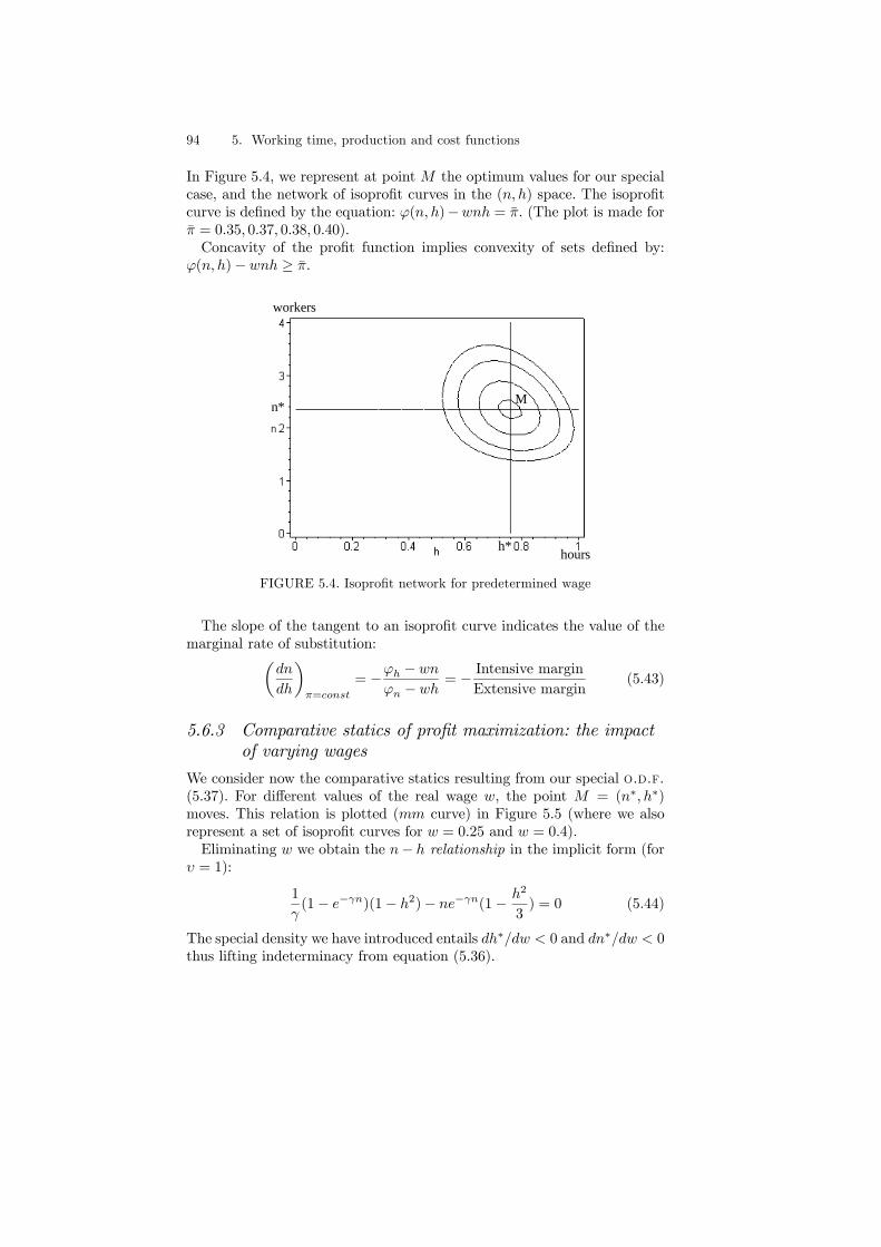
94 5. Working time, production and cost functions
In Figure 5.4, we represent at point M the optimum values for our specialcase, and the network of isoprofit curves in the (n, h) space. The isoprofitcurve is defined by the equation: ϕ(n, h)−wnh = π. (The plot is made forπ = 0.35, 0.37, 0.38, 0.40).Concavity of the profit function implies convexity of sets defined by:
ϕ(n, h)− wnh ≥ π.
M
h*
n*
hours
workers
FIGURE 5.4. Isoprofit network for predetermined wage
The slope of the tangent to an isoprofit curve indicates the value of themarginal rate of substitution:µ
dn
dh
¶π=const
= −ϕh − wn
ϕn − wh= − Intensive margin
Extensive margin(5.43)
5.6.3 Comparative statics of profit maximization: the impactof varying wages
We consider now the comparative statics resulting from our special o.d.f.(5.37). For different values of the real wage w, the point M = (n∗, h∗)moves. This relation is plotted (mm curve) in Figure 5.5 (where we alsorepresent a set of isoprofit curves for w = 0.25 and w = 0.4).Eliminating w we obtain the n− h relationship in the implicit form (for
υ = 1):
1
γ(1− e−γn)(1− h2)− ne−γn(1− h2
3) = 0 (5.44)
The special density we have introduced entails dh∗/dw < 0 and dn∗/dw < 0thus lifting indeterminacy from equation (5.36).

5.6 The two dimensional demand for labor with a specific g.p.f. 95
m
m
M (w = 0.25)
M' (w' = 0.4)
increasing wages
FIGURE 5.5. Optimal staff and working time under wage variation
5.6.4 On the impossibility of a decentralized equilibrium inthe labor market with a constant wage rate
The former analysis puts forward a possible source of conflict in the labormarket, if the wage rate is a linear price of labor. As shown, firms manifestan explicit demand for hours and workers; only, by fortunate coincidence,this two dimensional demand simultaneously matches the individual supplyof hours and the global supply of workers.More precisely, if profits are of the form π(n, h) = ϕ(n, h) − wnh, full
equilibrium requires the following conditions:
ϕn(n, h)− wh = 0 (5.45)
ϕh(n, h)− wn = 0 (5.46)
n = ns(w) (5.47)
h = hs(w) (5.48)
This system of four equations cannot generally be solved by three endoge-nous variables {n, h,w}.Figure 5.6 depicts possible configurations in the labor market when
ns(w) = n. The northeast quadrant represents the internal supply and de-mand for individual hours, the northwest quadrant represents the externalsupply (assumed constant for simplicity) and the demand for workers. Atthe external (full-employment) equilibrium (point B), insiders work longerthan desired hours; at the internal equilibrium (point A), unemploymentn−nA is observed. Obviously, in the case depicted in Figure 5.6, a perfectlyflexible wage would not be able to simultaneously eliminate rationing in theinternal and external markets.

96 5. Working time, production and cost functions
w
workers hours
wA A
B wB
45° m
m
hA hBnA
workers
n*(w) h*(w)
hs(w)n_
n_
real wage rate
FIGURE 5.6. Internal vs. external equilibrium
The elementary neoclassical case is the special situation in which thereexists a function F (, ) such that ϕ(n, h) = F (nh) ∀(n, h). In this caseϕn(n, h) = hF 0(nh) and ϕh(n, h) = nF 0(nh). The equality w = F 0(nh)eliminates simultaneously the extensive and the intensive margins, solvingthe first two equations of the former system.
5.7 Conclusion
In this chapter, focus was set on the complexity of the productive pro-cess. From a formal description, we evolved towards more tractable butreductive concepts emphasizing, however, the respective roles of hours andemployment. In the next chapters, generalized production functions andgeneralized cost structures will be extensively in use, a better knowledgeof these concepts being a basic precondition of a precise understanding ofactual labor contracts and of any prediction pertaining to the effects ofmandatory working time reductions.Mandatory working time reductions aim at increasing employment, in
a man-hours substitution process. In a decentralized economy, the firmsbeing able to subject employment to their profit maximization policy, we
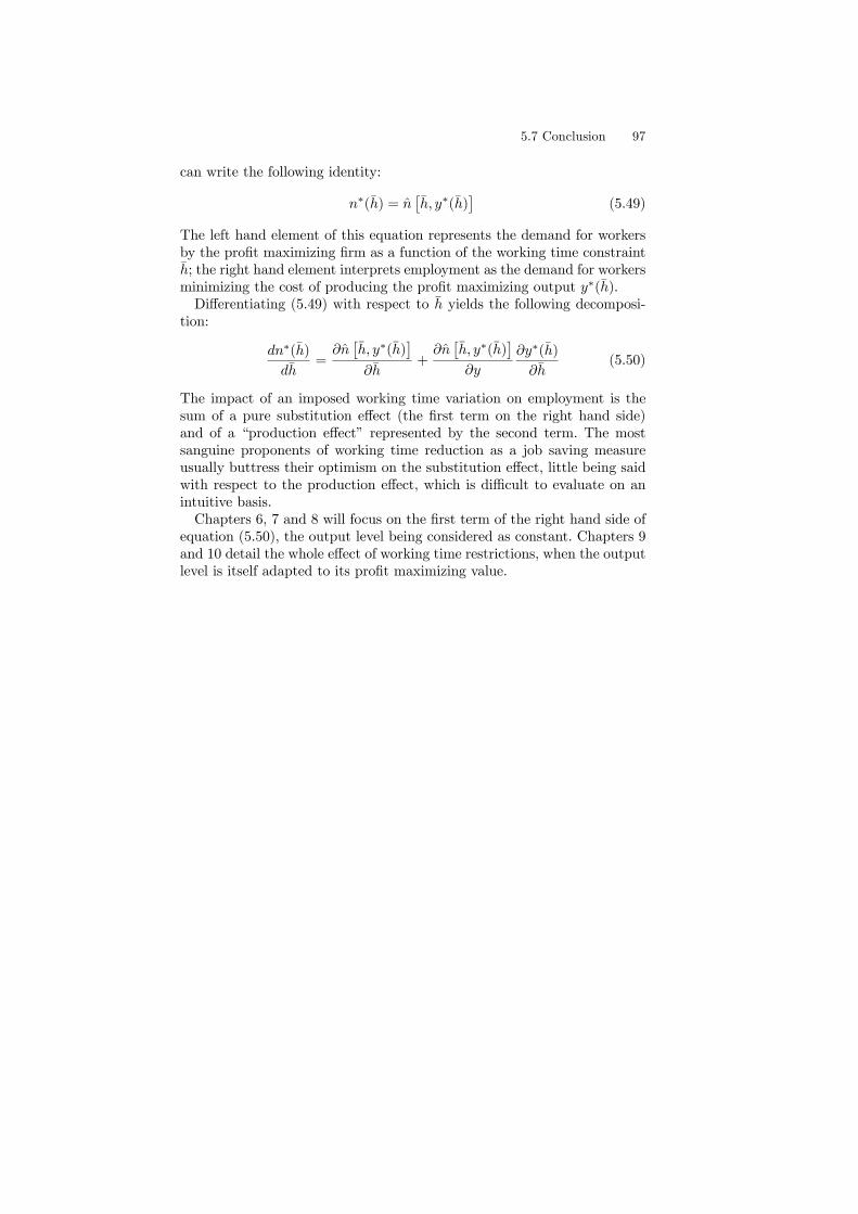
5.7 Conclusion 97
can write the following identity:
n∗(h) = n£h, y∗(h)
¤(5.49)
The left hand element of this equation represents the demand for workersby the profit maximizing firm as a function of the working time constrainth; the right hand element interprets employment as the demand for workersminimizing the cost of producing the profit maximizing output y∗(h).Differentiating (5.49) with respect to h yields the following decomposi-
tion:
dn∗(h)
dh=
∂n£h, y∗(h)
¤∂h
+∂n£h, y∗(h)
¤∂y
∂y∗(h)
∂h(5.50)
The impact of an imposed working time variation on employment is thesum of a pure substitution effect (the first term on the right hand side)and of a “production effect” represented by the second term. The mostsanguine proponents of working time reduction as a job saving measureusually buttress their optimism on the substitution effect, little being saidwith respect to the production effect, which is difficult to evaluate on anintuitive basis.Chapters 6, 7 and 8 will focus on the first term of the right hand side of
equation (5.50), the output level being considered as constant. Chapters 9and 10 detail the whole effect of working time restrictions, when the outputlevel is itself adapted to its profit maximizing value.

98 5. Working time, production and cost functions

This is page 99Printer: Opaque this
6Working time in a cost minimizationproblem
In Chapter 5, a formal approach helped to represent production processesand cost structures in a less simplified context than is usually assumed inconventional microeconomics. In this chapter, generalized production andlabor cost functions are applied to the general problem of labor expenseminimization by the firm. Cost minimization is always a necessary conditionfor profit maximization, but it may also apply directly to the “Keynesian”case, in which firms are constrained in the goods market, being able to sellonly limited quantities, at least in the short run. In this case, their optimaldecision is limited to choosing the minimum cost input mix.In section 6.1 we highlight the role played by fixed costs of labor only in
explaining the optimal labor contract from the firm’s point of view and theemployer’s tendency to extract longer hours than are willingly supplied bythe workers. Section 6.2 examines the particular case where the employeris constrained to provide workers with a working time duration equal totheir individual supply and emphasizes the inefficient character of this sit-uation. Section 6.3 introduces a slightly more elaborate model, where theproduction function is also generalized to allow for imperfect man-hourssubstitution.

100 6. Working time in a cost minimization problem
6.1 Neoclassical production function with fixedcosts of labor
We begin the analysis with a very simple model of working time determina-tion, where the principal extension of the traditional neoclassical analysisconsists in introducing a more general labor cost structure. As mentionedin Chapter 5, in a static framework, labor costs are made up of wage costsand various fixed costs proportional only to the number of people at work,but independent of working time.In this simple framework, the labor market is supposed to be competi-
tive. Firms must therefore submit labor contracts that workers are willingto accept, that is, must provide them with a utility level higher or equalto some reservation utility. This reservation utility level is open to vari-ous interpretations: in a perfectly homogeneous and flexible labor marketeconomy, this level should be understood as endogenous; it is an expres-sion of the satisfaction level obtained by workers at full employment andis a common constraint imposed on all firms. In other cases, with externalunemployment, it should be associated with unemployment compensationand with maximum leisure time. In more structured economies, the con-straining utility level would be the outcome of negotiations between unions,firms and the state, a kind of social contract.More formally, let us denote by s this minimum utility requirement.
Worker preferences may be represented by a neoclassical utility functionu = u(c, h), having as arguments consumption possibilities c and workingtime h. Following standard neoclassical assumptions, uc > 0, uh < 0. Thelength of the reference period will be normalized, which implies a maximumworking time h = 1.Then, condition u(c, h) ≥ s, often called ”participation constraint”, im-
plies an acceptancy region in the plane (Oc,Oh) bordered by a frontier c(h)implicitly defined by u [c(h), h] = s and defined in Chapter 4 as the “work-ing time compensating consumption function”. Following the neoclassicalparadigm, we assume that this compensating consumption is increasingand convex: c0(h) > 0, c00(h) > 0, with c(0) = c0 ≥ 0 and lim
h→1c(h) = ∞
(Figure 6.1).
With the participation constraint may be associated a reservation valueof the wage rate noted wr, defined as the minimum hourly wage rate con-vincing the employee to work; at this wage rate, workers’ hours supply hris the solution to the problem: min
h{c(h, s)/h} and corresponds to point R
in Figure 6.1.Labor expenses are therefore E = n(c + θ), where c is workers’ daily
compensation and θ stands for the fixed costs per worker; these costs havebeen discussed at length in Chapter 5.
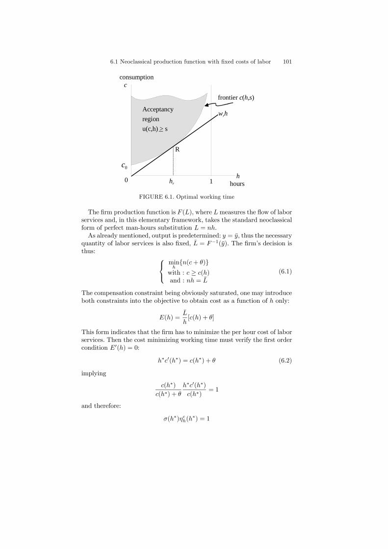
6.1 Neoclassical production function with fixed costs of labor 101
h
c
0 1
c0
Acceptancyregionu(c,h) > s_
consumption
hours
wrh
R
hr
frontier c(h,s)
FIGURE 6.1. Optimal working time
The firm production function is F (L), where Lmeasures the flow of laborservices and, in this elementary framework, takes the standard neoclassicalform of perfect man-hours substitution L = nh.As already mentioned, output is predetermined: y = y, thus the necessary
quantity of labor services is also fixed, L = F−1(y). The firm’s decision isthus: ⎧⎨⎩
minh{n(c+ θ)}
with : c ≥ c(h)and : nh = L
(6.1)
The compensation constraint being obviously saturated, one may introduceboth constraints into the objective to obtain cost as a function of h only:
E(h) =L
h[c(h) + θ]
This form indicates that the firm has to minimize the per hour cost of laborservices. Then the cost minimizing working time must verify the first ordercondition E0(h) = 0:
h∗c0(h∗) = c(h∗) + θ (6.2)
implying
c(h∗)
c(h∗) + θ
h∗c0(h∗)
c(h∗)= 1
and therefore:
σ(h∗)ηch(h∗) = 1

102 6. Working time in a cost minimization problem
where ηch(h) is the elasticity of the compensation function with respect toh and σ(h) is the ratio of wage cost to total labor cost per worker.Graphically, the solution may be easily illustrated using isocost lines, i.e.
the sets of values of c and h assigning a constant value E to the expenditure
function E =L
h[c+ θ]. An isocost line is defined by the explicit function:
c = −θ + E
Lh
It can be represented in the (Oc,Oh) plane by a straight line of slope (E/L)and crossing the vertical axis at c = −θ.The compensating consumption function and two isocost lines are rep-
resented in Figure 6.2. The decision of the firm is represented by point Fwhere the solid line is tangent to the compensatory consumption. It corre-sponds to the lowest cost E∗, compatible with workers’ acceptance of thelabor contract.
E diminishes
h
c c(h)c=-θ+(E*/L)h
h*
−θ
c(h*) F
0
FIGURE 6.2. Cost minimizing contract under utility constraint
It is easily seen from Figure 6.2 that the contract proposed by the firmin this setting has an efficiency property since at F, cost is minimizedunder the workers’ satisfaction constraint and equivalently, workers’ utilityis maximized under the cost constraint.

6.1 Neoclassical production function with fixed costs of labor 103
However, if we consider that workers’ compensation is delivered by meansof a linear wage, it can easily be shown that under this contractual arrange-ment, ∀θ > 0, they would prefer to work shorter hours (and earn a lowercompensation) than imposed by the firm.Let us denote by hs(w) the individual labor supply function, that is the
working time which maximizes the workers’ satisfaction for any wage rate,w.
hs(w) = argmaxh{u(wh, h)}
The hourly wage rate w∗ required to provide the optimal compensationc(h∗) is defined by c(h∗) = w∗h∗ and is equal to the slope of the straight linejoining the origin to the point F describing the firm’s decision (c(h∗), h∗).But as clearly shown in Figure 6.3, this configuration implies systematic
overwork, that is hs(w∗) < h∗. Obviously, the existence of fixed costs oflabor is sufficient to prompt firms to demand more than Walrasian workinghours. The point W representing the Walrasian supply by the worker andthe point F do not coincide.
h
c
0
c(h)c=-θ+(E/L)h
h*
−θ
c(h*)=w*h*
hs
F
W
FIGURE 6.3. Optimal contract: firm and worker point of view
Walrasian rationing of the insiders could be reduced by introducing amandatory constraint on working hours, h < h∗. In this framework, work-ers’ rationing would disappear at R where the hours constraint and the wage
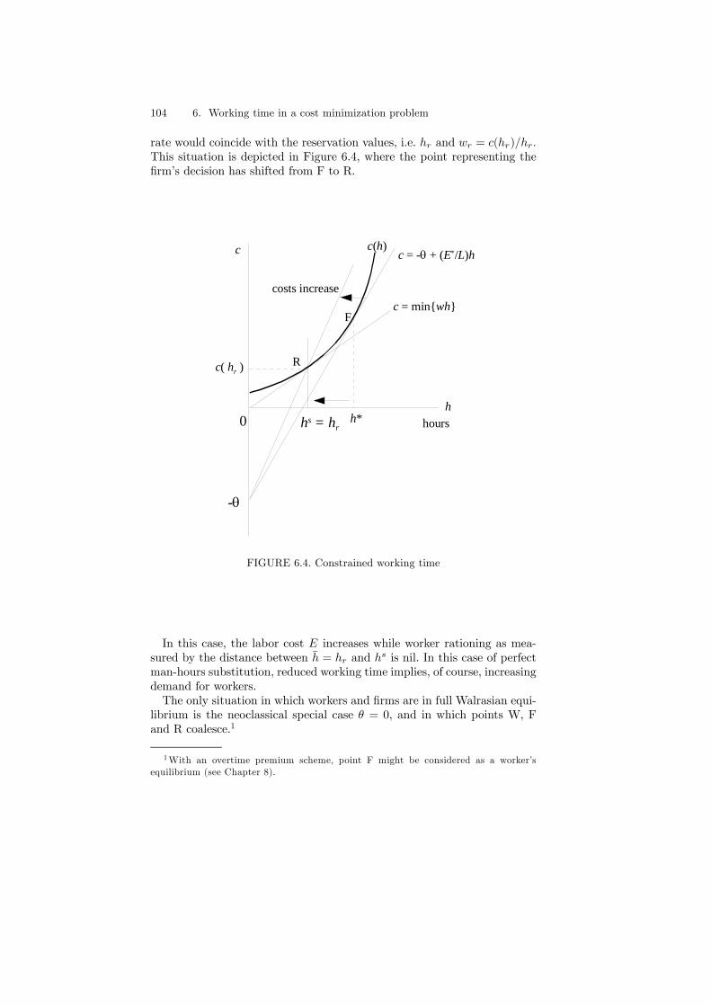
104 6. Working time in a cost minimization problem
rate would coincide with the reservation values, i.e. hr and wr = c(hr)/hr.This situation is depicted in Figure 6.4, where the point representing thefirm’s decision has shifted from F to R.
h
c
0
c(h)c = -θ + (E*/L)h
h*
c = min{wh}
hs = hr
-θ
costs increase
hours
c( hr )
F
R
FIGURE 6.4. Constrained working time
In this case, the labor cost E increases while worker rationing as mea-sured by the distance between h = hr and hs is nil. In this case of perfectman-hours substitution, reduced working time implies, of course, increasingdemand for workers.The only situation in which workers and firms are in full Walrasian equi-
librium is the neoclassical special case θ = 0, and in which points W, Fand R coalesce.1
1With an overtime premium scheme, point F might be considered as a worker’sequilibrium (see Chapter 8).

6.2 Consequences of supply determined working time 105
6.2 Consequences of supply determined workingtime
The situation in which the firms would be allowed to determine the hourlywage rate, but should comply with the number of hours optimally suppliedby the workers is worth further analysis. In this case, the output constrainedfirm (F (L) = y) solves the following cost minimization problem:⎧⎨⎩
minw{n[whs(w) + θ]}
with: w ≥ wr
and: nhs(w) = L
(6.3)
Substituting n with L/hs(w), the firm’s decision is represented by maxi-
mization of E(w) = L
∙w +
θ
hs(w)
¸.
For an interior solution, the first order condition E0(w) = 0 implies
θhs0(w)
[hs(w)]2= 1 (6.4)
or, in elasticity terms:
whs(w) = θηhs
w
or else:
σ =ηh
s
w
1 + ηhsw
where σ is the share of wage costs in total labor costs and ηhs
w the wageelasticity of the hours supply.The consequences of such a situation are depicted in Figure 6.5. The
feasible contracts are limited to the points of the RS curve where the util-ity of the worker is maximized for the current wage rate. Minimum totallabor cost may be obtained (interior solution) for the particular worker’sequilibrium W where the RS curve is tangent to an isocost straight line.The incurred labor cost is higher than at point F where the firm minimizescost by controlling wages and working time.
Comparative statics related to the fixed cost θ can explain how somesurplus from work may be obtained by the worker. In the absence of suchcosts, W clearly coincides with R and the worker is exactly compensated.For higher values of θ, point W moves upwards on the RS curve indicatingpositive surplus from work. From (6.4), this surplus appears if θ > θ0 =
[hs(wr)]2
hs0(wr). If θ increases indefinitely, (6.4)⇒ hs0(w) = 0, isocost lines tend

106 6. Working time in a cost minimization problem
h
c
0
c(h)
c = −θ + (E*/L)h
h*hr
-θ
hours
c( hr )
F
R
S
W
FIGURE 6.5. Optimal contract under hours supply constraint
to be vertical and the wage policy amounts to maximizing the individuallysupplied working time, in order to reduce the number of workers.Last but not least, the contract W is not efficient. At this point, it might
be shown that the indifference curve and the isocost line are not mutuallytangent and border a set of points yielding simultaneously more satisfactionto the worker and reduced labor costs. As inefficient contracts are highlyunstable, in the following developments of this book we concentrate on thecase of utility constraints on the decision of the firm.
6.3 A more general approach: labor effectiveness
This section extends the cost minimization problem under utility competi-tion to a more general form of the production function.
6.3.1 The cost minimization problem
As in the former case, the production function is F (L), with F 0(L) >0, F 00(L) < 0 where L are labor services. Here we consider that hours

6.3 A more general approach: labor effectiveness 107
and workers are no longer perfect substitutes in the production of laborservices. We hold however the multiplicatively separable form introducedin the former chapter: L = ng(h), where g0( ) > 0. Note that the elasticityof labor services with respect to workers ηLn = 1; the elasticity of labor
services with respect to hours ηLh =hg0(h)
g(h)= ηgh. Output is predetermined,
implying L = L. The labor cost function is: E(n, h) = n[c(h) + θ] wherec(h) represents worker compensation and θ are the fixed costs per worker.The cost minimization problem is therefore:(
minh,n
{n[c(h) + θ]}with: ng(h) = L
(6.5)
The Lagrangian L = {n[c(h) + θ]− λ[ng(h)− L]} entails first order condi-tions:
Ln = c(h) + θ − λg(h) = 0 (6.6)
Lh = nc0(h)− λng0(h) = 0 (6.7)
Lλ = ng(h)− L = 0 (6.8)
Dividing equation (6.7) by equation (6.6) we obtain the following form offirst order conditions applying to the cost minimizing working time h∗:
c0(h∗)
c(h∗) + θ=
g0(h∗)
g(h∗)(6.9)
In terms of elasticities, equation (6.9) may be written equivalently:
σ(h∗)ηch(h∗) = ηgh(h
∗)
with ηgh(h∗) =
h∗g0(h∗)
g(h∗), ηch(h
∗) =h∗c0(h∗)
c(h∗), and σ(h∗) =
c(h∗)
c(h∗) + θis the
share of wage costs in total labor costs.
6.3.2 Second order conditions
The conditions for cost minimization under output constraint with gener-alized production and cost functions have been detailed in Chapter 5, andapply here in the special setting at hand. They may be readily specifiedby considering the labor costs as a function of h only. Since ng(h) = L, we
can consider that the firm minimizes E(h) = Lc(h) + θ
g(h).

108 6. Working time in a cost minimization problem
At a point where the first order condition (6.9) holds, i.e. E0(h∗) = 0,the second order condition E00(h∗) > 0 is equivalent to:
c00(h)g(h) > g00(h) [c(h) + θ]
It is always fulfilled if g00(h) < 0. It may be fulfilled for positive values of
g00(h), if g00(h) < c00(h)g(h)
c(h) + θ.
6.3.3 Graphic solution
As in the case of prefect man-hours substitution, the solution h∗ can beobtained graphically by introducing the auxiliary concept of an isocostcurve. An isocost curve represents all the pairs (c, h) generating a givenlabor cost. Let us consider the expenditure function: E(n, h) = n[c(h) + θ]and substitute n by L/g(h). Then, a constant cost curve of E0 level isdefined by:
c =E0Lg(h)− θ (6.10)
Notice that the isocost curve has the same shape as the worker effectivenessfunction g(h). As explained in Chapter 5, this function may be convex forthe first hours, then become concave, given that exertion may justify posi-tive but decreasing contribution of additional hours to output. It interceptsthe vertical axis at −θ. The smaller the cost, the lower is the curve. There-fore, cost minimization necessitates establishing the lower isocost curve,consistent with the workers’ minimum satisfaction constraint. Figure 6.6shows the solution as the point F. The lowest isocost curve corresponds tothe minimum cost E∗. In this picture, workers still perform longer thandesired hours, h∗ > hs(w∗), as in the case of perfect man-hours substitu-tion. However, in the case of generalized production functions, this outcomeis no longer certain: Figure 6.7 shows the alternative situation of insiderunderemployment, in which workers would like to work longer than actualhours.
The workers’ supply and the firms’ demand for hours might coincide onlyin the exceptional case where the isocost curve is tangent to the compensa-tion function for a duration equal to the reservation hours, hr. In this case,the slope of the isoscost curve is equal to the slope of the compensationfunction and is equal to the reservation wage; points W and F coalesce.
6.3.4 An exercise of comparative statics
The impact of varying effectiveness and of fixed labor costs on the optimalduration is easily determined in the particular case where g(h) = hβ, β < 1.

6.3 A more general approach: labor effectiveness 109
h
c
0
c(h) c=-θ+(E*/L)g(h)
h*
−θ
c(h*)
hours
w*h*
hs
F
W
FIGURE 6.6. Optimal working time: overwork
Then condition (6.9) becomes:
c0(h∗)
c(h∗) + θ=
β
h∗(6.11)
Comparative statics of the equilibrium working time may be sketched withrespect to changes in the relevant parameters, i.e.: θ, related to the fixedcosts of labor and β, related to worker effectiveness in time.By differentiating equation (6.11), we show that for β < 1 an increase in
hour effectiveness contributes to increasing working time:
dh∗
dβ=
c(h∗) + θ
(1− β)c0(h∗) + h∗c00(h∗)> 0
ηh∗
β =βσ
ηch∗ [(1− β) + ηc0h∗ ]
> 0
σ being the share of wages in total labor cost. The elasticity ηc0
h∗ =h∗c00(h∗)
c0(h∗)is positive by the convexity assumption.As expected, an increase in the fixed cost of labor would push firms to
increase working time:
dh∗
dθ=
β
(1− β)c0(h∗) + h∗c00(h∗)> 0
ηh∗
θ =
µ1− σ
σ
¶β
ηch∗ [(1− β) + ηc0h∗ ]
> 0

110 6. Working time in a cost minimization problem
h
c
0
c(h)
c=-θ+(E*/L)g(h)
h*
−θ
c(h*)
hours
w*h*
hs
F
W
FIGURE 6.7. Optimal working time: insider underemployment
The response of employment to changes in parameters is important fora policy purpose. For a predetermined output, employment is implicitlygiven by: g(h∗)n∗ = L, thus
dn∗
dh∗= −n
∗g0(h∗)
g(h∗)
or in elasticity terms:
ηn∗
h∗ = −ηgh
Thus, any change in the parameter value which implies a reduction inequilibrium working time would also bring an increase in employment:
ηn∗
β = −ηghηhβ and ηn∗
θ = −ηghηhθthat is, increasing fixed costs and worker effectiveness would decrease thedemand for workers.
6.4 Cost minimization with factor substitution
6.4.1 The case with unconstrained working hours
In this subsection we consider more general situations, in which both cap-ital and labor services may be adjusted, output still being considered aspredetermined.

6.4 Cost minimization with factor substitution 111
Denoting by k the number of equipments units, the flow of capital servicesis K = kz(h), where z(h) is a “capital effectiveness function”. The functionz(h) captures the relationship between working time h and the flow ofservices from the capital endowment. It may be constant, increasing ordecreasing. In the simplest case, z(h) = h, implying that capital servicesare linear in hours, unmanned capital being unproductive.The technology is represented by the generalized production function:
y = F (K,L) = F [kz(h), ng(h)] (6.12)
where L represents labor services and has the already mentioned form,L = ng(h).We assume that the rental cost of capital is of the form (δ + r)k; the
depreciation of equipment does not depend upon the daily working time.Under these assumptions, the cost minimization problem is:(
mink,n,h
{k(r + δ) + n[c(h) + θ]}with: F [kz(h), ng(h)] = y
(6.13)
where c(h) is the compensating consumption function and θ are the fixedcosts of labor. The solution (n∗, k∗, h∗) should verify first order conditionsrelative to the Lagrangian form:
L = k(r + δ) + n[c(h) + θ]− λ{F [kz(h), ng(h)]− y} (6.14)
First order conditions applying to (6.14) are:
Ln = c(h) + θ − λg(h)FL = 0 (6.15)
Lk = r + δ − λz(h)FK = 0 (6.16)
Lh = nc0(h)− λ[kz0(h)FK + ng0(h)FL] = 0 (6.17)
From (6.15) and (6.17), we obtain a special condition for the solution h∗:
c0(h∗)
c(h∗) + θ=
g0(h∗)
g(h∗)+
K
L
FKFL
z0(h∗)
z(h∗)(6.18)
We denote the share of wage costs in total labor costs by σ(h). Defining
L(K) by F (K,L(K)) = y, we denote ηLK =K
LL0(K) = −K
L
FKFL
< 0. Then,
the former expression may be written in equivalent elasticity terms,
σ(h∗)ηch(h∗)− ηgh(h
∗) = −ηLKηzh(h∗) (6.19)
6.4.2 The impact of a mandatory reduction in working hours
In the following, we consider the effects of a binding constraint on workinghours, the law imposing a maximal duration, h ≤ h∗. As seen in Chapter 3,

112 6. Working time in a cost minimization problem
in the work-sharing paradigm, such a policy is expected to induce firms tosubstitute hours with workers. It must be noticed that in our assumptionsthe reduction of hours for given n and k implies a simultaneous reductionof labor and capital services.In this case, working time is no longer a control variable and first order
conditions (6.15) and (6.16) only apply; from them we can write an expres-sion for the ratio of marginal productivities of the two forms of services:
FKFL
=
µg(h)
z(h)
¶µr + δ
c(h) + θ
¶(6.20)
To explore the consequences of mandatory working time reduction, we in-troduce a simple homogeneous Cobb-Douglas production function: F (K,L)
= KαL1−α, implying ηLK = −KFKLFL
= − α
1− αand therefore:
FKFL
=
µα
1− α
¶µng(h)
kz(h)
¶(6.21)
From (6.20) and (6.21), k =µ
α
1− α
¶µc(h) + θ
r + δ
¶n.
Substituting k in the constraint y =£kz(h)
¤α £ng(h)
¤1−α, we obtain:
lnn = Const+ ln(y)− α ln[c(h) + θ]− α ln[z(h)]− (1− α) ln[g(h)](6.22)
Differentiating (6.22) with respect to h finally yields:
ηnh(h) = −ηgh(h)− αηzh(h)− α
£σ(h)ηch(h)− ηgh(h)
¤(6.23)
This last relation in elasticity terms shows the complexity of the responseof the cost minimizing firm to a mandatory working time reduction, whenthe quantity of productive capital is flexible. In some cases, equation (6.23)however takes a simpler form.For instance, if the constraint applies to an initially free system, (6.19)
holds and we can write σ(h∗)ηch(h∗) − ηgh(h
∗) = −ηLKηzh(h∗). Given thatin the case of the Cobb-Douglas form ηLK = −α/(1 − α), equation (6.23)becomes:
ηnh(h∗) = −ηgh(h∗)−
µα
1− α
¶ηzh(h
∗) (6.24)
It may be noted that the man-hours substitution which would take place ifcapital services were kept constant is indicated by the first term of the righthand side of equation (6.24). The impact of human working time on capitalservices is indicated by the elasticity ηzh. If the function z(h) is increasingin h, (ηzh > 0), men are needed to offset fewer hours and capital services.

6.5 Conclusion 113
If z(h) is decreasing in h, (ηzh < 0), man-hours substitution is limited inconsequence of increased capital services per time-unit. If we consider thesimple case in which z(h) = h, and therefore ηzh(h) = 1 ∀h, the elasticityof employment with respect to working time is:
ηnh(h∗) = −ηgh(h∗)−
µα
1− α
¶(6.25)
The additional effect of labor capital substitution on the elasticity ηnh(h)represented by α/(1−α) is a consequence of fewer capital services suppliedby a given stock of equipments when working hours are reduced.
6.5 Conclusion
The cost minimizing approach helps emphasize the role of fixed costs oflabor and of varying effectiveness in the determination of working time bythe firms, when they are constrained to offer contracts compatible with aminimum satisfaction of workers. It clearly reveals the possibility of varioustypes of insider rationing.When the production function is neoclassical (builds on the assumption
of perfect man-hours substitution), the mere existence of fixed costs ex-plains the employer’s tendency to require longer hours than are willinglysupplied.Introducing a more general description of production and allowing for
varying effectiveness, the model shows a more complex situation, in whichinsider rationing may go either way; in particular, if worker effectiveness intime decreases sharply, employers may prefer short working hours despitefixed costs per worker; in this case, the possibility of insider underemploy-ment, with workers working fewer than desired hours per period, cannotbe ruled out. This leads to a reversed conflict about working time.In the cost minimization framework, imposing a binding constraint on
working hours may contribute to increase the demand for workers, giventhe induced scarcity in labor and capital services. The measure is howeveraccompanied by a reduction in profits.The model at hand is a useful benchmark for more detailed analysis of
working time in the context of predetermined output. In the next chapter,we investigate the case of workers who are identically productive but havedifferent consumption/leisure preferences, and we put forward the optimalcontract offered by the firm.

114 6. Working time in a cost minimization problem
This is page 115Printer: Opaque this
7Cost minimization, heterogeneousworkers and asymmetric information
In Chapter 6, we considered homogeneous workers, not only in terms ofproductive skills but also in relation to their consumption/leisure prefer-ences. Firms were perfectly informed about workers’ characteristics anddetermined the optimal input mix given a unique participation constraintapplying to all of them. This chapter considers an extension of cost mini-mization problems, focusing on the design of optimal compensation schemeswhen workers differ only in terms of consumption/leisure preferences orreservation utility levels. In this generalized setting, a new issue arises: isthe employer entitled to offer a definite contract to a worker or a subset ofworkers exclusively? Such a policy, when it is feasible, is often termed “dis-criminatory”, identical labor services being finally paid differently. It mustbe noticed that the mainstream of economic analysis applied to discrimina-tion tends to define this concept in a restrictive way: there is discriminationif the same economically homogeneous good or service is sold (or bought) atdifferent prices. Most models of this tradition tend to account for differentwages applying to workers who are identical under all attributes includingtastes, apart from some economically irrelevant parameters such as sex orethnicity (see the survey by Cain 1986). Here, we consider discriminationas the ability of the firm to reserve different contracts for workers of thesame skill, but having varied working hours compensation demands.The feasibility of this cost minimizing policy depends firstly upon the le-
gal and institutional environment of the firm. In some countries, employersare given considerable freedom in their contracting practices and the prin-ciple of equal reward for equal work does not really apply. For instance, theFrench law tolerates unequal treatment of workers as a form of the right

116 7. Cost minimization, heterogeneous workers and asymmetric information
to manage in the private sector, except if the differences are based on sex,religion or race. Even in the case where discrimination is not forbidden on alegal basis, its application may be difficult, to the extent that worker typesare in general private information, unknown to the employer. In this situa-tion, the firm can only offer a set of contracts defining working time and itscompensation, and leave workers free to make their choice. This particularsetting is related to a standard category of problems usually included un-der the heading of “mechanism design”, and has been extensively studiedby recent microeconomic theory, in particular as applied to second pricediscrimination by the monopolist. The reader may find detailed analysesof this topic in Fudemberg and Tirole (1991, chapter 7) and Mas-Collel etal. (1995, chapter 14).The text is organized as follows. In the first section, we introduce the
main assumptions and the general Kuhn and Tucker conditions encompass-ing different particular types of solutions. Section 7.2 deals with the specialcase where some of the more demanding workers are left unemployed, firstin the discriminating case, then when discrimination is ruled out. The lastsection 7.3 investigates the implications of a policy of mandatory workingtime reduction.
7.1 The decision problem of the firm
7.1.1 Main assumptions and constraints
We consider the general problem of minimizing the cost of a given outputunder a set of constraints.a) Workers are clustered into a finite number of types, according to their
consumption/leisure preferences and their minimum utility requirementlevels. Preferences of the type i worker are represented by quasi-linear util-ity functions ui(ci, hi) = ci − vi(hi) where ci and hi respectively measurethe total wage compensation and the number of working hours per period.In each case vi(0) = 0, v0i(hi) > 0, and v
00i (hi) > 0. Each type of worker has
a reservation utility level si defined as the utility levels attainable outside,through unemployment benefits or other job opportunities. A contract isaccepted only if ci − vi(h) ≥ si.1
In the following, to keep the analysis as simple as possible, we considertwo types only: i = (1, 2). Then, the firm has to determine labor contracts(c1, h1) and (c2, h2) subject to participation constraints P1 and P2:
c1 − v1(h1) ≥ s1 (P1)
1Corneo (1995) analyzed the participation decision of heterogeneous workers accord-ing to their autonomous income.

7.1 The decision problem of the firm 117
c2 − v2(h2) ≥ s2 (P2)
b) If discrimination is impossible, incentive compatibility constraints mayalso appear, as a consequence of free contract choice by workers of alltypes. These constraints called IC1and IC2 are obtained by writing thatthe contract earmarked for one type of worker is at least as well appreciatedby this type as the contract designed for the other type; this implies in oursetting:
c1 − v1(h1) ≥ c2 − v1(h2) (IC1)
c2 − v2(h2) ≥ c1 − v2(h1) (IC2)
c) The amount of output to be produced is predetermined and requiresa quantity L of labor services. The technology is neoclassical in the sensethat hours and workers are perfect substitutes in the production of one unitof labor services. While workers differ regarding their consumption/leisurepreferences, they are homogeneous with respect to their effectiveness intime. Denoting by n1 (n2) the number of type 1 (type 2) workers, thequantity constraint, pertaining to the necessary amount of labor services isobviously binding in any case and holds as an equality:
n1h1 + n2h2 = L (QC)
d) We assume that workers of the first type are available in number n1,workers of the second type in number n2 . Then, availability constraints are
n1 ≤ n1 (AC1)
n2 ≤ n2 (AC2)
The objective of the firm consists in minimizing total labor costs:
E = n1c1 + n2c2 + θ(n1 + n2)
all the above mentioned constraints being fulfilled. As in previous chapters,we denote by θ the fixed cost per incumbent worker, whatever its type.Non-negative slack variables must be introduced where there are inequal-
ity constraints. If e1 and e2 stand for unemployed workers in each type,availability constraints AC are:
n1 + e1 = n1 (7.1)
n2 + e2 = n2 (7.2)
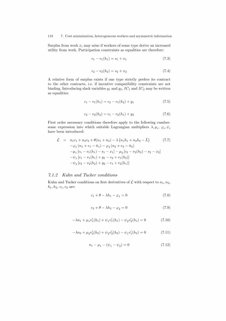
118 7. Cost minimization, heterogeneous workers and asymmetric information
Surplus from work xi may arise if workers of some type derive an increasedutility from work. Participation constraints as equalities are therefore:
c1 − v1(h1) = s1 + x1 (7.3)
c2 − v2(h2) = s2 + x2 (7.4)
A relative form of surplus exists if one type strictly prefers its contractto the other contracts, i.e. if incentive compatibility constraints are notbinding. Introducing slack variables y1 and y2, IC1 and IC2 may be writtenas equalities:
c1 − v1(h1) = c2 − v1(h2) + y1 (7.5)
c2 − v2(h2) = c1 − v2(h1) + y2 (7.6)
First order necessary conditions therefore apply to the following cumber-some expression into which suitable Lagrangian multipliers λ, µi, ϕi, ψihave been introduced:
L = n1c1 + n2c2 + θ(n1 + n2)− λ¡n1h1 + n2h2 − L
¢(7.7)
−ϕ1 (n1 + e1 − n1)− ϕ2 (n2 + e2 − n2)
−µ1 [c1 − v1(h1)− s1 − x1]− µ2 [c2 − v2(h2)− s2 − x2]
−ψ1 [c1 − v1(h1) + y1 − c2 + v1(h2)]
−ψ2 [c2 − v2(h2) + y2 − c1 + v2(h1)]
7.1.2 Kuhn and Tucker conditions
Kuhn and Tucker conditions on first derivatives of L with respect to n1, n2,h1, h2, c1, c2 are:
c1 + θ − λh1 − ϕ1 = 0 (7.8)
c2 + θ − λh2 − ϕ2 = 0 (7.9)
−λn1 + µ1v01(h1) + ψ1v
01(h1)− ψ2v
02(h1) = 0 (7.10)
−λn2 + µ2v02(h2) + ψ2v
02(h2)− ψ1v
01(h2) = 0 (7.11)
n1 − µ1 − (ψ1 − ψ2) = 0 (7.12)

7.2 Optimal contracts and working time 119
n2 − µ2 − (ψ2 − ψ1) = 0 (7.13)
Conditions related to non-negative slack variables e1, e2, x1, x2, y1, y2 are:
−ϕ1 ≥ 0 and e1ϕ1 = 0 (7.14)
−ϕ2 ≥ 0 and e2ϕ2 = 0 (7.15)
µ1 ≥ 0 and x1µ1 = 0 (7.16)
µ2 ≥ 0 and x2µ2 = 0 (7.17)
−ψ1 ≥ 0 and y1ψ1 = 0 (7.18)
−ψ2 ≥ 0 and y2ψ2 = 0 (7.19)
Conditions related to the Lagrangian multipliers are equivalent to the con-straints.
7.2 Optimal contracts and working time
The above system is compatible with a variety of situations. In the fol-lowing, we will focus on an interesting case, where some workers of themore demanding type 1 are unemployed. The availability constraint is notbinding, implying ϕ1 = 0. It can be checked that the hourly wage rateis necessarily higher for this type, since from equations (7.8) and (7.9),c1h1= λ− θ
h1and
c2h2= λ+
ϕ2 − θ
h1with ϕ2 < 0.
The decision problem of the firm must be considered in two different situ-ations according to the feasibility or impossibility of discrimination amongworkers.
7.2.1 The discriminating case
We can first consider the basic subproblem in which the firm is able toassign different contracts to different workers. Incentive compatibility con-straints do not apply and participation constraints are necessarily bothbinding.2 In this case, equations (7.8) to (7.19) hold with ψ1 = ψ2 = x1 =x2 = 0.
2 In the event of a positive surplus for one type, cost could be reduced by the employerin decreasing compensation for this type in keeping with all the constraints.

120 7. Cost minimization, heterogeneous workers and asymmetric information
From (7.12) and (7.13), n1 = µ1 and n2 = µ2; therefore (7.10) and (7.11)imply:
v01(h1) = v02(h2) = λ (7.20)
Finally, (7.8) and (7.9) may be written:
c1 = h1v01(h1) + ϕ1 − θ (7.21)
= h1v01(h1)− θ
c2 = h2v02(h2) + ϕ2 − θ, with ϕ2 < 0 (7.22)
This solution is depicted in Figure 7.1 where points F1 and F2 illustratethe cost minimizing contracts. The contract F1 is equivalent to labor costminimization of labor services obtained from type 1 workers, a problemthat has been analyzed at length in Chapter 6.
As in this analysis, the minimum cost per type 1 worker is obtained atthe tangency point between the indifference curve at the reservation leveland the lower isocost line. Unlike the former analysis, the quantity of laborservices demanded is endogenous.Let us denote the solution to the general problem h∗1, h
∗2, n∗1 and n
∗2 = n2,
with L∗1 = n∗1h∗1 and L∗2 = n∗2h
∗1. Whatever L∗1, the cost of these la-
bor services has been minimized. Constant costs for type 1 workers imply
n1(c1 + θ) = E1, entailing isocost lines of equation: c1 = −θ +E1L∗1
h1. The
firm seeks to minimize E1 under the constraint c1−v(h1) > s1. The lowestcost is obtained at the tangency point F1 between the indifference curveat the reservation level and the less abrupt isocost line (the slope at theisocost lines increases with costs).We know from condition (7.20) that at the optimum, the slopes of the
indifference curves are identical. Then, the other point F2 is obtained byshifting this isocost line to the right, until it reaches the tangency pointwith the indifference curve of the type 2 workers. Notice that with discrim-ination, no worker retains any surplus from work.The multiplier λ coincides with the wage rate ci/hi only for a type of
worker in excess supply (ϕi = 0) and in the special case where the firmincurs no fixed labor costs θ = 0. In such a case, the employer pays thereservation wage rate of this type and working time coincides with its Wal-rasian supply.
7.2.2 Non-discriminating contracts
When discrimination is ruled out, workers choose among the proposed con-tracts so as to maximize their satisfaction and the incentive compatibility
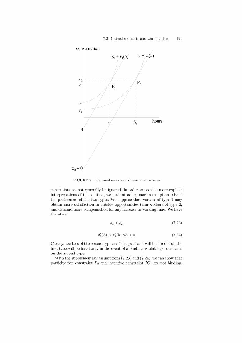
7.2 Optimal contracts and working time 121
consumption
hoursh1 h2
c2
c1
s1
s2
−θ
ϕ2 − θ
F1
F2
s1 + v1(h) s2 + v2(h)
FIGURE 7.1. Optimal contracts: discrimination case
constraints cannot generally be ignored. In order to provide more explicitinterpretations of the solution, we first introduce more assumptions aboutthe preferences of the two types. We suppose that workers of type 1 mayobtain more satisfaction in outside opportunities than workers of type 2,and demand more compensation for any increase in working time. We havetherefore:
s1 > s2 (7.23)
v01(h) > v02(h) ∀h > 0 (7.24)
Clearly, workers of the second type are “cheaper” and will be hired first; thefirst type will be hired only in the event of a binding availability constrainton the second type.With the supplementary assumptions (7.23) and (7.24), we can show that
participation constraint P2 and incentive constraint IC1 are not binding.

122 7. Cost minimization, heterogeneous workers and asymmetric information
To show that P2 is not binding, we note that from (7.5) c2 − v2(h2) ≥c1 − v2(h1), since v1(0) = v2(0) = 0, (7.24) ⇒ v1(h) > v2(h) ∀h > 0,therefore c1−v2(h1) > c1−v1(h1). Then, (7.3)⇒ c1−v1(h1) ≥ s1 and from(7.23), s1 > s2. Therefore c2−v2(h2) > s2. In the absence of discrimination,one category of workers may reap a surplus from work.Since P2 is not binding, IC2 is necessarily binding (otherwise the firm
could reduce labor cost by reducing c2). Suppose that the two incentivecompatibility constraints are simultaneously binding, (7.5) and (7.6) withy1 = y2 = 0 would imply: v1(h2)−v1(h1) = v2(h2)−v2(h1), in contradictionto (7.24). IC1 is therefore not binding and P1 is binding.On this set of assumptions, Kuhn and Tucker conditions (7.8) to (7.19)
hold with: x1 = 0, µ1 > 0; x2 > 0, µ2 = 0; y2 = 0, ψ2 > 0; y1 > 0, ψ1 = 0.In such a case, the following equations obtain:
µ1 = n1 + n2 (7.25)
λ = v02(h2) (7.26)
n2 = υ2 (7.27)
Under these assumptions, we can state several interesting propositions.
Proposition 6 Type 1 workers are requested to work fewer hours than type2.
Proof. Introducing equations (7.25), (7.26) and (7.27) in (7.10) yields:
v01(h1) =n1v
02(h2) + n2v
02(h1)
n1 + n2(7.28)
This last equation shows that either v02(h1) < v01(h1) < v02(h2) or v02(h1) >
v01(h1) > v02(h2) but (7.24)⇒ v02(h1) < v01(h1) and the second case must berejected. We have therefore:
v02(h1) < v01(h1) < v02(h2) (7.29)
Since v02(h1) < v02(h2),
h1 < h2 (7.30)
Proposition 7 When some workers of type 1 are unemployed, ruling outdiscrimination entails a shorter working time for incumbent workers of thistype.

7.2 Optimal contracts and working time 123
Proof. In this case, ϕ1 = 0, and condition (7.8) holds under the form:
c1 = λh1 − θ (7.31)
The binding participation constraint is:
c1 = s1 + v1(h1) (7.32)
Then, equations (7.31) and (7.32) imply:
v1(h1) = λh1 − (θ + s1) (7.33)
In the discriminating case, equation (7.33) is satisfied with λ = v01(h1). Inthe non-discriminating case, it is satisfied with λ = v02(h2). From (7.29)v02(h2) > v01(h1) or v
02(h2) = v01(h1) + α, where α > 0. Noting by hd1 the
discriminating solution and by hnd1 the non-discriminating solution, we canwrite:
v1(hd1) = hd1v
01(h
d1)− (θ + s1) (7.34)
and
v1(hnd1 ) = hnd1
£v01(h
nd1 ) + α
¤− (θ + s1) (7.35)
The last two equations, and α > 0 imply:
v1(hnd1 )− hnd1 v01(h
nd1 ) > v1(h
d1)− hd1v
01(h
d1) (7.36)
The function g1(h) ≡ v1(h) − hv01(h) is monotonously decreasing since itsderivative is g01(h) = −hv001 (h) < 0. In this case, condition (7.36)⇒ hnd1 < hd1
We represent in Figure 7.2 the case in which the first type of worker isin excess supply (ϕ1 = 0) and fixed costs are neglected (θ = 0). Points F1and F2 characterize the discriminating solution that has already been de-picted in Figure 7.1; points F 01 and F
02 indicate the non-discriminating case;
moving from F1 to F 01 implies increasing the cost of labor services obtainedfrom type 1, this increase being offset by a reduced incentive compatibil-ity constraint applying to the contract designed for type 2. Consequently,cnd1 = hnd1 v02(h
nd2 ) and cnd2 = hnd2 v02(h
nd2 ) + ϕ2 with ϕ2 < 0.
It may be seen that in F 01, the type 1 worker would like to work more ata constant wage rate, and in F 02 workers of type 2 would like to work less.
7.2.3 The case of non-binding incentive compatibilityconstraints
When discrimination is feasible, constraints IC1 and IC2 do not apply.Ruling out discrimination however does not imply that incentive compati-bility constraints are necessarily binding. In some instances, the firm is able
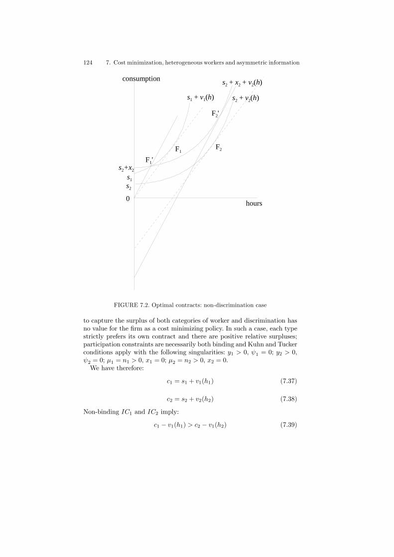
124 7. Cost minimization, heterogeneous workers and asymmetric information
consumption
hours
s1s2
F1F2
s1 + v1(h) s2 + v2(h)
F1'
F2'
s2+x2
s2 + x2 + v2(h)
0
FIGURE 7.2. Optimal contracts: non-discrimination case
to capture the surplus of both categories of worker and discrimination hasno value for the firm as a cost minimizing policy. In such a case, each typestrictly prefers its own contract and there are positive relative surpluses;participation constraints are necessarily both binding and Kuhn and Tuckerconditions apply with the following singularities: y1 > 0, ψ1 = 0; y2 > 0,ψ2 = 0; µ1 = n1 > 0, x1 = 0; µ2 = n2 > 0, x2 = 0.We have therefore:
c1 = s1 + v1(h1) (7.37)
c2 = s2 + v2(h2) (7.38)
Non-binding IC1 and IC2 imply:
c1 − v1(h1) > c2 − v1(h2) (7.39)
7.2 Optimal contracts and working time 125
c1 − v1(h1) > c2 − v1(h2) (7.40)
Substituting c1 and c2 in (7.39) and (7.40) with their expressions in (7.37)and (7.38) yields the following inequalities:
s1 + v1(h1) < s2 + v2(h1) (7.41)
s1 + v1(h2) > s2 + v2(h2) (7.42)
These two inequalities are compatible only with crossing indifference curves,as represented in Figure 7.3.
consumption
hours
s1
s2
F1=F1'
s1 + v1(h)
s2 + v2(h)
F2=F2'
0
FIGURE 7.3. Non-binding incentive constraints
Crossing indifference curves may therefore explain optimality and feasi-bility of different wage rates for workers having the same productive abilitiesbut different preferences, and not submitted to any discriminating pressure.In the case depicted in this subsection, the cost minimizing policy set
up by the employer is compatible with a working time structure of thewage rate which looks like a premium pay for overtime scheme. This mayprovide a theoretical background for the empirical analysis by Hart andRuffel (1993) who have analyzed the highly deregulated labor market inthe United Kingdom and put forward the emergence of spontaneously ne-gotiated contracts with an overtime structure.3
3Premium schemes for long hours are investigated in Chapter 8.

126 7. Cost minimization, heterogeneous workers and asymmetric information
7.3 Legal interference on working time
As put forward in subsection 7.2.2, in the absence of discrimination, thecost minimizing design links the contracts offered to the two different typesof workers. In this section we consider the consequences of a superimposedundifferentiated legal limit to working hours, denoted h. Legal reduction(dh < 0) cannot change employment of type 2 workers who are all em-ployed, but is intended to foster employment of the first type who are inexcess supply. We have seen in Proposition 6 that h1 < h2. In such a case,a (not too strong) legal constraint may be directly binding only for type 2.We know that employment and working time of the two types are there-
fore related by the labor services constraint:
n1h1 + n2h = L (7.43)
In differentiating (7.43), the elasticity of employment n1 with respect to hmay be decomposed in the following way:
ηn1h= −L2
L1− ηh1
h(7.44)
where L1 = n1h1 and L2 = n2h. The policy of working time reductionwould obviously contribute to increase employment (of type 1 workers) ifthe second term ηh1
hwere nil. Unfortunately, under a mandatory working
time reduction the optimum working time exacted from type 1 workersmay increase. The second term ηh1
his thus negative and tends to offset
the man-hours substitution effect. If the ratio L2/L1 is small, this adverseeffect would dominate the favorable substitution effect.This may be established in the following terms. In the proximity of h2,
constraints P1 and IC2 remain binding, and the problem of the cost min-imizing firm is in our set of assumptions (we assume away fixed costs forsimplicity) equivalent to:
min{E = n1c1 + n2c2}
under constraints:n1h1 + n2h2 = L, h2 = h, n2 = n2, (IC2) ⇒ c2 − v2(h2) = c1 − v2(h1)
and (P1)⇒ c1 = v1(h1) + s1.After substitutions, the objective may be expressed as a function of h1
only:
E(h1) =L− n2h
h1[v1(h1) + s1] + n2
£v1(h1) + s1 + v2(h)− v2(h1)
¤(7.45)
First order condition on (7.45) implies:
L− n2h
h1
∙v01(h1)−
v1(h1) + s1h1
¸+ n2 [v
01(h1)− v02(h1)] = 0 (7.46)

7.4 Conclusion 127
The general comparative statics showing the effect of varying h on theoptimal value h1 solution of (7.45) is cumbersome. For a simpler treatment,we suggest introducing the quadratic proxies v1(h) = α1h
2 and v2(h) =α2h
2 with α1 > α2. In this case, it may be shown that (7.46) takes theform: ¡
L− n2h¢ ¡s1 − α1h
21
¢= 2n2(α1 − α2)h
31 (7.47)
In Figure 7.4, the left hand side of this equation and the right hand sideare represented as functions of h1. Their intersection (point A) determineson the horizontal axis the cost minimizing value of h1.
hours, type 1h1
))(( 21112 hshnL α−−
0
31212 )(2 hn α−α
0<∆h
A
A'
FIGURE 7.4. Hours constraint and the optimal duration
Decreasing h clearly shifts the curve representing the left hand side up-wards, implying increasing working hours for the workers of the first type;the elasticity ηh1
his therefore negative.
7.4 Conclusion
Introducing diversity of preferences in cost minimization problems revealsnew properties of optimal labor contracts. When firms do not know thetrue characteristics of the workers, or if the law precludes discriminatoryattitudes, the employer’s problem amounts to offering a cost minimizing setof labor contracts that motivates workers to freely reveal their preferences,by selecting the contract devised for their type. Moreover, in such a case, theresponse of the productive sector to a mandatory hours constraint applyingto those most inclined to accept long hours may have disappointing effectson total employment, insofar as it implies an increased number of hoursworked by the type of workers initially working fewer hours.

128 7. Cost minimization, heterogeneous workers and asymmetric information
The next chapter introduces the analysis of legal overtime paymentschemes often superseding the individual participation constraint.

This is page 129Printer: Opaque this
8Premium pay for overtime
8.1 Institutional schemes and possible supplyresponse
In many countries, legislated schemes interfere with labor contracts by im-posing a well-defined working time structure on the wage rate. In the UnitedStates, for instance, the Fair Labor Standard Act requires applying a 50%premium on hours worked each week beyond a threshold of 40 hours. Inmany other instances, working time regulations also impose a two-partcompensating system, in which hours exceeding some statutory level arepaid at a premium wage rate.Such regulated paying schemes may be represented by the following form:
wage rate =½
w, for h ≤ h0aw, for h > h0
(8.1)
i.e., a normal wage rate applies to hours up to a threshold h0, firms hav-ing to pay a times this normal wage for hours exceeding this threshold.In some countries, two successive thresholds are defined and determine theapplication of different (increasing) premium rates. In some cases, upperbounds on absolute durations of work have also been adopted. Hours pay-ment schemes often include many other elements of complexity, describedin detail in OECD, Employment Outlook, 1998.Worker coverage by these schemes varies from one country to another
(see Table 8.1).

130 8. Premium pay for overtime
Percentage of workersaccepting overtime
Overtime(hours per week)
Australia 32.1 2.7Canada 17.0(c) 1.4Finland 10.6 0.9France 14.0 ...
Germany(a) ... 1.2Italy ... 5.0Japan ... 3.4UK(b) 53.3 5.3US ... 4.2
TABLE 8.1. Overtime in manufacturing, selected countries, 1996. (a) all sectors;(b) male employment. Sources: OECD, Employment Outlook, 1998. For France:DARES, Monthly Labor Survey, 1996. For the US: Bureau of Labor Statistics.(c) from Duchesne (1997)
Table 8.2 at the end of the chapter describes the basic elements of suchregulations in various countries.What rationale lies behind such a widespread intervention of public au-
thority? Mandatory overtime payment schemes are most often vindicatedby different arguments:— An overtime premium increases the relative cost of supplementary
hours obtained from insiders compared with hours supplied by outsideworkers. When the firm faces peak demand on the goods market, it istherefore encouraged to hire new workers, reducing unemployment. Thisargument clearly resorts to the work-sharing paradigm in a dynamic con-text. For transitory activity increases, specific costs incurred by the firm inrelation to changing numbers of workers creates an incentive to require theneeded hours from the insiders. The overtime payment premium applyingto them tends to counterpoise such cost of change, shifting the labor costminimizing policy of the firm in favor of outsiders.— In pure statics, mandatory overtime premium may be understood as
protecting workers against the consequences of contracts they might ac-cept, but deemed individually or socially detrimental by the authoritiesthemselves. Too many hours of work may slowly ruin individuals’ healthor prevent them from investing in education or child rearing. Such behav-ior may be considered as detrimental to the development of the society inthe long run and this form of market failure would appear if workers havea shorter planning horizon (life-time) than policy makers (several gener-ations). In such a case, the law on working time pursues its own welfareobjectives and aims at protecting workers against themselves.An interesting question consists in conjecturing what would happen in
the absence of such regulations. As we have seen in Chapter 6, competitionamong firms compels them to design contracts providing workers with a
8.1 Institutional schemes and possible supply response 131
minimum utility level. If workers have neoclassical preferences, the feasi-ble working contracts would exhibit a time increasing wage rate structure.The compensatory wage function c(h) being convex, the effective compen-satory wage rate w(h) = c(h)/h would be increasing. The mandatory over-time premium scheme could therefore be interpreted as an institutionalarrangement which approximates workers’ preferences while economizingon the complexity and transaction costs of private negotiations.The study by Hart and Ruffel (1993) would corroborate this hypothesis.
They found that in the highly deregulated British economy where contractsand pay for overtime are freely negotiated between employers and work-ers in many sectors, the observed schemes are consistent with an overtimepremium proportional to the basic wage rate. “In general however, whilecomplicated non-monotonic relationships are possible, the marginal over-time premium of the individual worker may be typified either as a constantor as a rising step function of overtime hours” (Hart and Ruffel, 1993,p.184). Their estimations of the negotiated premium are close to 1.5. Itturns out that the working time structure of the wage rate negotiated inthe free labor market of the United Kingdom is close to the a priori legis-lated scheme in the United States. In Japan, regulation is more permissive,requiring a 1.25 times premium; Hart et al. (1996) showed that for verylong working weeks, the negotiated marginal premium in this country risesto 1.32.1
Another possible interpretation for such freely negotiated premium payfor overtime agreements may be suggested by our analysis in Chapter 7:when the firm must recruit heterogeneous workers in terms of preferences,but does not have the right or practical possibility to discriminate amongthem, in some cases the incentive constraints may not be binding and theresulting optimal agreements coincide with a two-part wage rate.As a first important consequence, overtime premium rules should affect
the hours supply behavior. If we represent the worker’s decision as thesolution of the problem:⎧⎨⎩ max {u(c, h)}
with½
c = wh, if h ≤ h0c = wh0 + aw(h− h0), if h > h0
(8.2)
it is easily checked that the feasible set in the space (Oh,Oc) is no longerconvex. In this case, the solution of problem (8.2) may not be unique andthe comparative statics on h0 or a reveal individual discontinuity in thesupply behaviorIt must be noticed, however, that the overtime premium scheme may
also be interpreted as restoring a Walrasian equilibrium when the contract
1See also Bell and Hart (1998) for a detailed observation of overtime patterns in theUK.

132 8. Premium pay for overtime
devised by the firm minimizes the cost of labor under the worker’s utilityconstraint. As has been shown in Chapter 6, with fixed cost of labor θ, thecost minimizing labor contract F is not compatible with Walrasian supplyW for the effective wage rate (Figure 8.1). But point F as a worker’s equi-librium may be supported by an infinity of overtime premium rules as in(8.2) corresponding with varied w and h0, provided that aw = c0(h). Suchwage structures do not change the cost minimizing contract, but make itpossible to decentralize efficient transactions under the form of equilibri-ums.
h
c
0
c(h)
h*
c = wh
hs
-θ
hours
FW
h0
c = wh0 + aw(h - h0)
FIGURE 8.1. Premium wage for overtime and the hours supply
Comparative statics on a for given values of w and h0 may be understoodstatistically, for a given population. For different values of a, individualsupply may switch from h < h0 to positive overtime h > h0. Empiricalestimates have been attempted from US cross-sectional data by Idson andRobins (1991). They find that an increase of a from 1.5 to 2 will onlyincrease the probability that a worker will offer to work overtime from0.2999 to 0.3032, implying a negligible impact of this increment on thesupply side.In the following developments of this chapter, we take a closer look at the
employment effect of this regulation on the demand for workers. The anal-

8.2 Premium pay for overtime in a cost minimization set-up 133
ysis will be carried out in the cost minimization framework where outputis taken as given by the firm.
8.2 Premium pay for overtime in a costminimization set-up
In this chapter we analyze the employment and hours decision of a firmwhose output is predetermined, an economic context that has already beenintroduced in Chapter 6.2 The firm is a “price taker” in a broad sense,since it considers the wage rate as predetermined, either determined by atrade union or resulting from some form of equilibrium in the labor market.Technology is represented by some production function F (L), where laborservices L take the multiplicative form L = ng(h), n being the number ofworkers and g(h) an effectiveness function.The legal daily compensation schedule is represented by a piecewise linear
function in worked hours. Then, allowing for a premium pay for overtime,it takes the form:
χ(h) =
½wh, if h ≤ h0
wh0 + aw(h− h0), if h > h0
with a > 1. The function χ(h) is therefore convex, presenting a kink forh = h0. Although this expression describes daily compensation as an in-creasing function in hours of work, it should be clearly distinguished fromthe compensating consumption function c(h) introduced in Chapters 4 and6, and utilized throughout this text. The compensation function c(h) isa pure consequence of workers’ consumption/leisure preferences and of aminimum demanded utility level; the function χ(h) is an exogenous ruleonly representing a legal constraint, given a predetermined “normal” wagerate w. In the following, we consider that the legal premium rule only isbinding, the participation constraint being not binding.The basic labor cost function is therefore:
E(n, h) = n[χ(h) + θ]
where and θ are the fixed costs per worker.If output is predetermined, then the required labor input is also exoge-
nous, L = L. In this case, using ng(h) = L, the cost function takes the
form: E(h) =L
g(h)[χ(h) + θ].
The first order condition E0(h) = 0 necessarily applies to the cost min-imizing duration h∗ if h∗ 6= h0. It can easily be shown that this optimal
2Alternative analyses of this subject are available in texts by Hart (1987) or Cahucand Zylberberg (1996).

134 8. Premium pay for overtime
number of hours verifies:
χ0(h)
χ(h) + θ=
g0(h)
g(h)(8.3)
A graphic solution may also be suggested, after introducing the auxiliaryconcept of isocost curve (defined in Chapter 6). In space (Oh,Oc), the pairs
(h, c) implying a constant cost E0 verify E0 =L
g(h)[c+θ]. Then, an isocost
curve is explicitly defined by c =E0Lg(h)− θ (previous equation 6.10). Its
shape is easily derived from g(h); since g(0) = 0, it intersects the verticalaxis in −θ. Lower constant cost levels define lower isocost curves on thegraph. The solution (h∗, c∗) to the cost minimization problem is depictedin Figure 8.2. It represents the case where supplied working time exceedsthe statutory hours, but, of course, the corner where solution h∗ = h0 mayalso obtain. It is worth noticing that in the traditional neoclassical case,the efficiency function being linear, g(h) = h, isocosts are straight lines andthis corner solution h∗ = h0 necessarily obtains.
h0 h*
−θ
χ(h*)
hoursh0
slope = aw
χ(h)
c= −θ + (E*/L)g(h)_
c
FIGURE 8.2. Cost minimizing hours
Explicit solutions may be obtained for specific effectiveness functions.We suggest considering the efficiency function introduced by Hart (1987):for h > τ, g(h) = (h− τ)β , with β < 1 to account for some exertion effect,and τ ≥ 0 being interpreted as a set-up time. Then equation (8.3) takes

8.3 Comparative statics on hours 135
the form:
aw
[wh0 + aw(h− h0)] + θ=
β
h− τ
and implies a cost minimizing working time:
h∗ =βθ + awτ − wh0β(a− 1)
aw(1− β)(8.4)
It must be kept in mind that the cost minimizing solution explains de-mand determined working time. It may not be feasible if it does not provideworkers with a sufficient utility level; in other words if the participationconstraint is not satisfied by the solution (h∗, χ(h∗)) . In some cases, theparticipation function and the legal constraint may be simultaneously bind-ing. It may be checked graphically that the solution may not be efficient,i.e. may not minimize labor costs for constant workers’ satisfaction.
8.3 Comparative statics on hours
We are now able to analyze the impact of varying the premium coefficienta and the statutory duration h0 on the optimal working time.In the standard neoclassical case g(h) = h and with fixed costs of labor,
the cost minimizing working time coincides with the threshold h∗ = h0.In this case, a reduction of the threshold obviously reduces the hours de-manded, while increases in a have no effect on h∗.We have shown that in the case of the concave efficiency function g(h) =
(h − τ)β for h > τ, (β < 1), the worker may undertake overtime hours.From equation (8.4), we have:
∂h∗
∂a= −β(θ + wh0)
wa2(1− β)< 0 (8.5)
or, in equivalent elasticity terms,
a
h∗∂h∗
∂a= − (θ + wh0)
(θ + wh0) + aw(τ/β − h0)< 0
As expected, an increase in the wage premium should reduce the optimalnumber of demanded hours.This sort of reaction has been empirically confirmed by Hamermesh and
Trejo (1999). We have seen that under the Fair Labor Standards Act, thefederal law in the United States requires that hours of work beyond 40hours per week should be paid time and a half. California was one of thefew states having imposed additional restrictions. In local regulations, Cal-ifornia has required for many years that most women receive an overtime

136 8. Premium pay for overtime
premium of 50% of the normal wage, for time exceeding eight hours a day.Starting from 1980, the same regulation has been extended to men, creat-ing favorable circumstances to test the impact of this measure on workedhours. According to the estimates by the authors, a 1% increase in theovertime premium is responsible for a 0.5% reduction in overtime hours.On the other hand, keeping the same assumptions in the form of the ef-
fectiveness function, it may be shown that reducing the statutory thresholdh0, for constant wage rate and premium ratio, would increase demandedworking hours, since from (8.4):
∂h∗
∂h0= −β(a− 1)
a(1− β)< 0 (8.6)
Such a response is not especially intuitive, but can easily be illustrated bymeans of Figure 8.3.
h0
χ(h)
h1*
−θ
hoursh0h2*
c
FIGURE 8.3. Impact of reducing statutory hours
8.4 Conclusion
For a constant activity level, supposing for instance price rigidities andKeynesian equilibrium, the cost minimizing models could provide someclues from which can be inferred the response of the productive sector interms of employment to changing parameters of the wage scheme. Suchchanges modify the cost minimizing working time h∗ and have an oppositeeffect on employment.

8.4 Conclusion 137
Indeed, the relationship between working time and employment is easilyobtained by differentiating the labor services constraint L = ng(h). For aconstant level of labor services, we can write:
dL = g(h)dn+ ng0(h)dh = 0
which implies the following negative elasticity of the demand for workerswith respect to working hours:
ηnh ≡h
n
dn
dh= −hg
0(h)
g(h)≡ −ηgh < 0 (8.7)
General a priori predictions should be avoided since assumptions aboutthe form of the efficiency function play a dominant role. The models mayonly help determine which relevant parameters in particular should be es-timated in order to obtain the conditional predictions of comparative stat-ics. Cost minimization models give some insights into more general settingssince any profit maximization policy requires cost minimization; more de-pendable comparative statics should however be claimed from models inwhich activity levels are endogenous, i.e. under the assumption of profitmaximization.

138 8. Premium pay for overtime
Statutoryweeklyhours
Premium wagefor overtime(in excess of normal hours)
Maxi-mumweeklyhours
Australia 38—4050% the first 4 hoursthen 100%
void
Austria 40 50% 50Belgium 40 50% (100% during the weekend) 60Canada 40—48 50% voidCzech Rep. 40.5 25% 51Denmark 37 50% the first hour, then increasing 48Finland 40 50% the first 2 hours, then 100% 45France 39 25% the first 8 hours, then 50% 48Germany 48 25% 60
Greece 4025% the first 60 hours per year50% the other 60 hours
48
Hungary 40 50% 52Ireland 48 25% 60Italy 48 25% 60Japan 40 25% voidKorea 44 50% 56Luxemburg 40 25% blue collars, 50% white collars 48Mexico 48 100% 57Netherlands 45 no regulation 60New Zealand 40 no regulation 48Norway 40 40% voidPortugal 40 50% the first hour, then 75% 50Spain 40 ... 54Sweden 40 no regulation 47Switzerland 45 (50) 25% 48 (52)Turkey 45 50% 61 (66)UK ... collectively bargained voidUS 40 50% void
TABLE 8.2. Overtime regulation in selected countries, 1996. Source: OECD, Em-ployment Outlook, 1998

This is page 139Printer: Opaque this
9Working time in a profitmaximization framework
9.1 Introduction
We have so far obtained general results by describing and interpreting theterms of labor contracts, using detailed descriptions pertaining to laborcost structures or working efficiency functions in the general framework ofcost minimization. All these results necessarily hold in the case of profitmaximization, for the profit maximizing output level.The productive sector, however, may be considered either as working
under an output constraint justified by some form of price rigidity as as-sumed in conventional Keynesian economics, or as optimally adjusting theactivity to its profit maximizing value. This second point of view is oftenconsidered as more representative of long run reactions in the productivesector where rigidities may be overcome.In this new chapter, as in the cost minimization approach (Chapter 6),
the production function is generalized to account for imperfect substitu-tion between workers and hours. We consider that firms must provide therepresentative worker with a minimum utility level to be obtained from atwo-dimensional labor contract, determining simultaneously his or her con-sumption and leisure time. This utility constraint level is first consideredin an unemployment context as predetermined, either by some unspecifiedinstitutional force, or by the utility level obtained out of work — dependingmainly on the prevailing terms of the unemployment benefits. The situa-tion in which the minimum requirements are flexible and decrease in thepresence of outside unemployment is then considered; in this pure market

140 9. Working time in a profit maximization framework
economy, the minimum utility level is endogenous. This approach may beviewed as an attempt to generalize the endogenous equilibrium wage rateof standard textbook analysis.1
Under our assumptions, it is shown how the terms of the labor contract,(hours and wage rate) as well as the employment level, are jointly deter-mined. Different configurations are possible from the worker’s point of view,ranging from overwork (working more than desired for the going wage), toinsider’s underemployment (working less than desired). Comparative stat-ics makes it possible to infer the impact of varying labor effectiveness, fixedcosts of labor, or an exogenous utility level on the explained variables. Fi-nally, the effect of mandatory working time reductions on the employmentlevel is examined. While pointing out the complex relationship betweenlabor effectiveness, fixed costs of labor, and demand for workers when thehours of work are constrained, the model developed here shows that if alimit on the duration of work is imposed on an initially free system, afirst favorable effect on employment might be achieved for a constant util-ity level of workers. For a particular production function, it is shown bymeans of a numerical simulation that further applications of the constraintmay decrease the employment level after reaching a maximum value. Conse-quently, only a too “strong” working-time constraint would have a perverseeffect on the demand for workers.Since unemployment is usually compensated with resources levied on
the firm’s wage bill, we finally introduce an elementary small size versionof the equilibrium model in which a government operates under a balancedbudget constraint. The authorities determine the level of unemploymentbenefits. For given consumption/leisure preferences, this welfare level ofthe unemployed determines the terms of the participation constraint ofthe workers. The tax rate to be applied on paid wages in order to exactlyfinance unemployment benefits results from this welfare objective and fromthe actual unemployment level; it is therefore an endogenous variable.The chapter is organized as follows. Section 9.2 reformulates the basic as-
sumptions about workers’ consumption/leisure preferences, cost structureand the productive process, which have already been developed in generalterms in previous chapters. Equilibrium working time, wage rate and em-ployment are analyzed in section 9.3. The impact on employment of a cut inthe legal working time is investigated in section 9.4. Section 9.5 sketches therole of endogenous payroll taxes in a simple general equilibrium framework.
1This chapter is a modified version of “A model of working time under utility com-petition in the labor market” published in the Journal of Economics (Zeitschrift fürNationalöekonomie), vol. 67, 1998, by the authors.

9.2 Main assumptions 141
9.2 Main assumptions
9.2.1 The workers’ consent to work
The workers’ utility function is neoclassical: u = u(c, l), where c standsfor the daily consumption flow and l for the daily leisure time. Moreover,c = wh, where h is the daily working time and w the real wage rate. Then,h + l = 1 (using the day as time unit) and the utility function can berewritten as: u = u(wh, 1− h).The following axioms describe the preferences of workers:
Axiom 8 Strong non-satiation and strict quasi-concavity implying respec-tively: u1 = ∂u/∂c > 0 u2 = ∂u/∂(1 − h) > 0 and convexity of any set inthe (Oc,Ol) space such that u(c, l) ≥ u0.
Axiom 9 Workers accept only the contracts providing them with at leasta utility level noted s.
The condition u(wh, 1 − h) ≥ s defines thus in the (Oh, Ow) spacean acceptance region, bounded by a frontier represented by the function:w = w(h, s). That is w(h, s) is implicitly defined by:
u(wh, 1− h) = s (9.1)
We call w(h, s) the hours compensating wage rate function; for any pre-determined s, it represents the minimum wage rate firms must pay in orderto determine workers to accept an h-hours contract (while granting themthe utility level s). In the following, s being explicitly assumed constant,we note w(h) = w(h, s). (This concept is related to the concept of “hourscompensating consumption function”, such as defined in Chapter 6, wherec(h) ≡ hw(h).)
Axiom 10 Individual preferences are consistent with a convex acceptanceregion, implying w00(h) > 0.
Notice that the quasi-concavity assumption on u(c, l) is not sufficient fora convex acceptance region in (Oh, Ow) space.
Axiom 11 We also assume that extreme values of the daily working timeimply infinite values of w0(h), i.e.: h → 0 ⇒ w0(h) → −∞ and h → 1 ⇒w0(h)→∞.
All these assumptions are consistent with many neoclassical utility func-tions, for instance the multiplicative form: u(wh, 1 − h) = wh(1 − h). Itshould be noticed that such utility functions embody relevant features ofconsumption/leisure preferences since any increase in resources due to alonger working day should compensate not only the direct nuisance inducedby the extra work but also the reduction in leisure time which prevents theindividual from enjoying his consumption possibilities.

142 9. Working time in a profit maximization framework
One may remark that for any w, the utility function u(, ) allows us todefine the individual Walrasian labor supply, i.e. the optimal working timefrom the worker’s point of view for a given wage rate:
hs(w) = argmaxh{u(wh, 1− h)} (9.2)
Under the former set of assumptions, it is possible to state the followingrule in terms of the compensating wage rate function:
Proposition 12 The contract {w(h), h} proposed by the firm coincides
with workers’ Walrasian labor supply hs(w) if w0(h) =µdw
dh
¶u=s
= 0; it
involves overwork if the contract implies longer hours than the Walrasian
supply h > hs(w) if w0(h) =µdw
dh
¶u=s
> 0 and insider underemployment
h < hs(w) if w0(h) =µdw
dh
¶u=s
< 0.
Proof. Differentiating u(wh, 1 − h) = s yields the slope of the com-
pensatory wage function w0(h) =
µdw
dh
¶u=s
=u2 − wu1
hu1. The first or-
der consequence of any variation dh of worked hours for a constant w is:
du = (u1w − u2)dh. Workers’ Walrasian supply requiresµdu
dh
¶w=Cst
=
0 and consequently w0(h) =
µdw
dh
¶u=s
= 0. For w0(h) 6= 0 two cases may
arise. Since hu1 > 0, w0(h) =µdw
dh
¶u=s
> 0 ⇒ (wu1 − u2) < 0, imply-
ingµdu
dh
¶w=Cst
< 0: the utility of the worker would be increased by a
reduced working time at the going wage (overwork prevails). Conversely,
w0(h) =
µdw
dh
¶u=s
< 0⇒ (wu1 − u2) > 0, implyingµdu
dh
¶w=Cst
> 0: the
worker would welcome increased working hours (insider underemploymentprevails).Figure 9.1 suggests an intuitive explanation in the case w0(h) > 0. Two
first curves are represented: w(h, s) is the compensatory wage function for
the competitive utility level s and w0(h) =
µdw
dh
¶u=s
is the subsequent
marginal utility with respect to hours. The latter is an increasing func-tion, given the assumption on the convexity of the compensatory wagecurve. Let us consider a working time h such that w0(h) 6= 0. In order tomotivate workers to accept this duration, the firm should pay them thewage rate w(h, s). But for this wage rate workers would like to work onlyhs[w(h, s)], and get a higher utility level s. The third upper curve repre-

9.2 Main assumptions 143
sents the compensatory wage function for this desired utility level, w(h, s).As hs[w(h, s)] < h, overwork prevails.
w(h,s)
10hours
w w'(h,s)w(h,s)
w(h,s)
h
^
~
hr hs
wr
FIGURE 9.1. Compensating wage function and workers’ rationing
We also represented the reservation wage wr; the worker would not sup-ply positive hours if the wage rate falls below this threshold. Of course, if
w0(h) =
µdw
dh
¶u=s
< 0, the opposite situation of insider underemployment
occurs, i.e. hs[w(h, s)] > h.
9.2.2 Generalized technology
Generalizing the neoclassical paradigm, we consider technologies in which,due to fatigue or other factors, workers and hours (in logarithms) are notperfect substitutes. This can be done by integrating a production functiony = F (L) — where y stands for output and L for labor input, with standardproperties F (0) = 0, F 0( ) > 0, F 00( ) < 0, but defining the labor input as aflow of labor services: L = ng(h) where n is the number of people at workand g(h) is the labor effectiveness function (see Chapter 5). We considerincreasing functions g0(h) > 0,∀h. A local property of the effectivenessfunction is its elasticity with respect to working hours, i.e.: ηgh = hg0/g.
144 9. Working time in a profit maximization framework
We also consider a generalized cost (or expenditure) function taking byassumption the two-part simplified form:
E = (wh+ θ)n, with θ > 0, (9.3)
where wnh is the linear part of the wage bill and θn captures the variouscosts depending only on the number of people at work.
9.3 The optimal contract: wages and hours
9.3.1 Profit maximizing under the workers’ utility constraint
By assumption, enterprises maximize profits in a goods market in full com-petitive equilibrium. In the labor market, firms are “utility-takers”, thelabor contract (wage, hours) providing workers with a minimum utilitylevel denoted s.The firm decision problem is thus:(
maxw,n,h
{π(w, n, h) = F [ng(h)]− wnh− θn}with: u(wh, 1− h) ≥ s
Using alternatively the former concept of compensatory wage function, w =w(h, s) denoted for simplicity w = w(h), the problem can be reconsidered asan unconstrained maximization in only two variables, the utility inequalityconstraint being obviously saturated:
maxn,h
{π(n, h) = F [ng(h)]− w(h)nh− θn} (9.4)
First order conditions are expressed in terms of extensive (πn) and intensiveprofit margins (πh):
πn = g(h)F 0 [ng(h)]− hw(h)− θ = 0 (9.5)
πh = ng0(h)F 0 [ng(h)]− nhw0(h)− nw(h) = 0 (9.6)
A solution of problem (9.4) is a labor contract {h∗, w(h∗)} and an optimumemployment level n∗ as implicitly determined by (9.5):2
g(h∗)F 0 [n∗g(h∗)]− h∗w(h∗)− θ = 0
2For a predetermined utility level, n∗ may be consistent with the existence of unem-ployed persons. The case where unemployment pushes the utility constraint down to thepoint of external equilibrium will be analyzed later on.

9.3 The optimal contract: wages and hours 145
To gain additional insight into the solution, we introduce the already de-fined elasticity of the labor effectiveness function ηgh and eliminate F
0( ) inequations (9.5) and (9.6):
w0(h∗) = ηghθ
(h∗)2− (1− ηgh)
w(h∗)
h∗(9.7)
(Second order conditions are scrutinized in Appendix I.)According to Proposition 12, if w0(h) > 0, overwork prevails; if w0(h) = 0
workers provide the Walrasian supply; if w0(h) < 0 insiders are submittedto underemployment.According to equation (9.7), ηgh ≥ 1 ⇒ w0(h) > 0 and overwork is the
only configuration possible.The absence of worker rationing requires w0(h) = 0, implying:
ηghθ
h2− (1− ηgh)
w(h)
h= 0 (9.8)
This condition can only be satisfied for ηgh < 1 since (9.8) implies:
ηgh =h∗w(h∗)
θ + h∗w(h∗)< 1 (9.9)
It must be noticed that for ηgh < 1 the three situations (overwork, Walrasiansupply, insider underemployment) are possible, insiders’ underemploymentbeing the likely outcome of small values of ηgh.To bring out more clearly the determinants of the labor contract, we can
write equation (9.7) in a slightly different form:
w0(h∗) = ηghθ
(h∗)2+ (1− ηgh)
∙−w(h
∗)
h∗
¸(9.10)
Equation (9.10) reveals a basic feature of the profit maximizing contractderived from the first order conditions: the first derivative of the compen-satory wage function must coincide with a weighted average of the twowell-defined functions θ/h2 and −w(h)/h. It applies to fixed or variablelabor effectiveness elasticities and lends itself to a graphic illustration help-ing to bring out clear comparative statics. Drawing in Figure 9.2 the twocurves θ/h2 and −w(h)/h in the (Oh,Ow) space, we represent the righthand side of equation (9.10) as a combination of the two curves respectivelyweighted by ηgh and (1− ηgh) named ZZ. The case of a constant elasticityηgh = η ∈ ]0, 1[ yielding a convex combination is used in the suggestedcurve.The solution is observed at the intersection A of ZZ and w0(h).3
3We cannot rule out another intersection between ZZ and w0(h), indicating a possiblemultiplicity of solutions especially for small values of η and θ. Contrary to FitzRoy(1993), this multiplicity is not general. As shown in Appendix II, in the domain whereg00(h) < 0 the profit function is concave and therefore can admit only one maximum.

146 9. Working time in a profit maximization framework
The situation of overwork would prevail for high fixed costs and/or ηghclose to (or higher than) one, as the curve ZZ would cross the w0(h) curvein its positive region. The reverse situation, of insider underemployment,would emerge for low fixed costs and/or low ηgh.It must be noticed that the wage rate in this model is entirely determined
by the labor effectiveness function, the worker’s preferences and fixed costsof labor. As in most efficiency wage models, this wage rate appears discon-nected from the marginal productivity, or more generally from the formof the production function (Solow, 1979). Of course, this last result stemsfrom our assumption in which the services of labor L are multiplicativelyseparable in workers and hours.
w(h)/hw'(h)
10 h*
A θ
h²
hours
w, w' θ
ZZZ'Z'
-w(h)/h
A'
FIGURE 9.2. Labor contract setting: the general case
Some comparative statics can be sketched in Figure 9.2. An increase inη is represented by an upward shift of ZZ towards Z0Z0 unambiguouslyincreasing working time and the wage rate.

9.3 The optimal contract: wages and hours 147
An increase in fixed cost θ also shifts the ZZ curve upwards and thereforeincreases h∗. Appendix II shows in analytical terms that the sign of thesensitivities of employment and working time to variations of the fixedcosts is well defined: dn∗/dθ < 0 and dh∗/dθ > 0.
9.3.2 The special case of perfect man-hours substitution
When η = 1, as implicitly assumed in the neoclassical standard case, equa-tion (9.10) takes the simple form w0(h) = θ/h2. In this case, the ZZ curveand θ/h2 coalesce, yielding the situation depicted in Figure 9.3, where over-work would prevail.
w(h,s)
w'(h,s)
10 h*
θ
hours
w, w'h²θ
h
w(h,s)
s
w(h*)
~
A
FIGURE 9.3. The case of perfect man-hours substitution
The segment BC = h∗ − hs(w∗) measures an unavoidable gap betweenthe optimal working time in the workers’ view and the optimal workingtime in the firm’s view. Only in the elementary version of the neoclassicalcase when θ = 0 and w0(h) = 0 does the firm’s optimal duration match theworkers’ Walrasian supply.

148 9. Working time in a profit maximization framework
Overtime work at a premium wage rate could be introduced at this stage.The cost of a worker being only related to its consumption claim c(h) =hw(h), the firm determines the optimal working time h∗ and has to paythe compensating consumption c(h∗) = h∗w(h∗). As mentioned in Chapter8, this consumption can be achieved by a family of non linear wages of theform:
c(h∗) = w0h0 + aw0(h∗ − h0), if h∗ > h0 (9.11)
where h0 separates regular and premium hours and aw0 (with a > 1) isthe premium wage rate. With more parameters under its control, the firmis able for instance to eliminate overwork in choosing a particular value for
w0 =u1 [c(h
∗), 1− h∗]
au2 [c(h∗), 1− h∗], h0 being fixed in accordance with (9.11). When
legal constraints impose h0 and a, the firm may not generally be able tofully eliminate the insider rationing. It is important to notice that optimumworking time from the firm’s point of view and the compensating consump-tion associated with this duration are independent of the payment scheme.In the following, we limit ourselves to the linear wage rate specification.
9.3.3 The full-employment utility level
The former analysis can be extended to the situation where the worker’srequirements are flexible, unemployed outsiders being able to bid downthe utility constraint level. In this case, outside equilibrium between thedemand and the supply for workers determines the constraining utility leveldenoted uE compatible with full employment.This type of situation may be analyzed by the simulation of a simplified
case with g(h) = hβ (implying ηgh = β). The computations use a particu-lar neoclassical production function F (n, h) = Q
¡nhβ
¢αand a particular
utility function which entails the above mentioned property of a convexacceptance region: u(wh, 1− h) = wh(1− h). This utility function impliesa compensatory wage function: w(h) = s/(h− h2).Figure 9.4 depicts two isoprofit networks in the plane (Oh,On) of equa-
tion π(n, h) = constant, the first obtained for s = 1, the second fors0 = 0.65. The other parameters have been assigned the following values:Q = 100, α = 0.75, β = 0.9, θ = 30. Points A and A0 indicate the profitmaximizing demand for workers and hours corresponding respectively to sand s0.When considering variations in the utility constraint level, the point A
which describes the labor contract offered by the unconstrained firm slidesalong a positively sloped curve denoted qq0. For instance, a reduction inthe utility level shifts the point A to A0.
This exercise makes it possible to infer some interesting properties of theexternal (full-employment) equilibrium. Consider a constant labor force,

9.4 Effect of a mandatory reduction of working time 149
workers
hours
q
q'
A(s =1)
A'(s' =0.65)
hE
n_
.
.
decreasingutility
increasingutility
FIGURE 9.4. Flexible utility level and outside equilibrium
n. Without a legal hour constraint, full-employment will be obtained atpoint E when workers’ utility demands uE are weak enough to fulfill thecondition: n∗ = n. At this point, the full-employment working time hE isindicated by the qq0 curve.The full-employment real wage rate is implicitly determined by first order
conditions. For instance, we can write from (9.5):
wE =g(hE)
hEF 0 [ng (hE)]−
θ
hE(9.12)
This expression encompasses as a special case the standard rule w = F 0(L)when g(h) = h and θ = 0. The labor contract is compatible with overworkor insider partial unemployment along the terms indicated by equation(9.10).
9.4 Effect of a mandatory reduction of workingtime
The model makes it possible to analyze the effects on employment of amandatory reduction in working hours. We first study the sensitiveness ofemployment to infinitesimal working time reductions, then we investigatethe employment path for any value of the working time constraint.

150 9. Working time in a profit maximization framework
9.4.1 Sensitivity of employment to small variations of theconstraint
Let us consider that an upper limit h is set on the duration of work, withh < h∗. The firm must pay the wage w(h) and its decision is limited to thechoice of the optimal value of n, denoted n.The first order condition (9.5) implicitly defines n:
πn = g(h)F 0£ng(h)
¤− hw(h)− θ = 0 (9.13)
By differentiating (9.13) one can determine the sensitivity of the demandfor workers with respect to h:
dn
dh= −ngg
0F 00 + g0F 0 − (w + hw0)
g2F 00= −πnh
πnn(9.14)
The sign and size of this expression indicate the local efficiency of manda-torily reducing the working time. From (9.6), we know that g0F 0 − (w +hw0) =
πhn= 0 when h coincides with its profit maximizing value h∗, but
g0F 0 − (w+ hw0) > 0 when the constraint is binding and the sign of (9.14)is therefore indeterminate.However, when the mandatory reduction applies to an initially free sys-
tem, the effect of the measure is easily determined. Since g0F 0−(w+hw0) =0, equation (9.14) ⇒ dn
dh= −ng
0
g, the elasticity of the demand for workers
with respect to h is:
ηnh = −ηgh
This incipient value coincides with the sensitiveness already obtained inthe context of output constrained behavior (Chapter 6).When working time is already constrained, g0F 0 − (w + hw0) > 0, thus
the terms of the man-hours substitution indicated by equation (9.14) maybe less favorable to employment.In the light of the former analysis, the legal reduction of working time in
an unconstrained system leads first to an increase in employment.
9.4.2 Employment as a function of the working timeconstraint
Equation (9.13) implies F 0[ng(h)] = [hw(h) + θ]/g(h), leading to:
n(h) =1
g(h)F 0−1½hw(h) + θ
g(h)
¾(9.15)
Equation (9.15) brings out an important structural feature of the economy,i.e. the relationship between the working time constraint and employment,

9.4 Effect of a mandatory reduction of working time 151
under constant worker utility. The precise shape of this function depends ong(h), F (L) and w(h). A thorough global analysis would therefore requireprecise knowledge of these three relevant functions. Consequently, n(h)could, a priori, have local or global extrema for h ∈ ]0, 1[ .From equation (9.14) it appears that maximizing employment n by a
working time constraint implies, for an interior solution, the first ordercondition:
dn
dh= 0⇒ ngg0F 00 + g0F 0 = (w + hw0) (9.16)
Denoting the elasticity of the marginal productivity with respect to laborservices ηF
0
L = LF 00/F 0, the elasticity of the compensating wage with re-spect to hours ηwh = hw0/w, the elasticity of output with respect to hours
ηFh =dF
dh
h
F= hng0F 0/F and labor’s share of output ψ = wnh/F (ng(h)),
equation (9.16) takes the form:
ψ (1 + ηwh ) = ηFh
³1 + ηF
0
L
´(9.17)
This first order condition is not sufficient and one cannot rule out the pos-sibility of the multiplicity of extrema of the function (9.15), in the generalcase.
9.4.3 A simple simulation
The existence of an interior global maximum of the former function isillustrated by a simple simulation using the already mentioned particularneoclassical production function: F (n, h) = Q
¡nhβ
¢αand the particular
utility function: u(wh, 1− h) = wh(1− h). In order to analyze the impactof the hours constraint, in Figure 9.5 we draw first the isoprofit networkin the plane (Oh,On) of equation π(n, h) = constant. Parameters wereassigned the same values as before, Q = 100, β = 0.9, α = 0.75, θ = 30. Inparticular, the utility constraint is set to s = 1.The slope of a given isoprofit curve is dn/dh = −πh/πn. It is indeter-
minate (takes the form 0/0) at the point A where the profit is maximizedwithout constraint. When the time constraint is binding, the firm choosesthe number of workers which maximizes profits (in keeping with the firstorder condition (9.13): πn = 0 ).In Figure 9.5, the time constraint is represented by a vertical line and the
employment constrained choice is the point where this vertical is tangentto an isoprofit curve. For various levels of the constraint the employmentchoice follows the curve denoted mm0. This last curve represents the graphof n(h). Of course, the point A belongs to mm0 since n(h∗) = n∗.

152 9. Working time in a profit maximization framework
workers
hours
AB
h*hB
_
m
m'
.
FIGURE 9.5. Working time constraints and the employment path
It can be checked that, as indicated by equation (9.14), in the neighbor-hood of A the mandatory reduction in working hours implies an increasein the demand for workers and a decrease in profits; in addition, for “low”durations of work, the terms of the substitution man/hours worsen and therelationship is inverted. Consequently, maximum employment is reached fora particular value of the working time constraint. In the simulation, thismaximum employment level, denoted B on Figure 9.5, is equal to 11.59 fora duration of work hB = 0.81, which can be compared with the uncon-strained choice (point A), where n∗ = 11.45 and h∗ = 0.84.
9.5 Working time reduction under predeterminedunemployment benefits
It is worth considering a situation in which the authorities simultaneouslycontrol the unemployment benefits and working time. Interesting investi-gations pertaining to the multiplicity of solutions of similar systems maybe found in FitzRoy et al. (1999). We restrict our analysis to a very sim-ple model in which the productive sector comprises f identical competitivefirms. Technology is still represented by y = F [ng(h)].The government determines a working time constraint h ≤ h.

9.5 Working time reduction under predetermined unemployment benefits 153
The workers (in number N) are identical. They accept working contracts(c, h) if u(c, h) ≥ u(b, 0) where b stands for the unemployment benefits inconsumption units. This participation constraint defines a working timecompensatory wage rate w(h, b) such that u {hw(h, b), h} = u(b, 0). Thiscompensatory wage function is increasing in b.The government determines the unemployment benefit level b = b, and
applies a flat tax rate τ on the cost of labor service to levy the correspondingresources. Unemployment is U = N − fn, and the government budgetconstraint implies:
b(N − fn) = τfnhw(h, b) (9.18)
Under the participation constraint, each firm maximizes its profit π =F [ng(h)]−nhw(h, b)(1+ τ); we suppose that in the solution, the intensivemargin is positive ng0(h)F 0 [ng(h)]− n(w + hwh)(1 + τ) > 0; the workingtime constraint is therefore binding, and h = h. The only control variablefor the firm is employment n; the competitive hypothesis entails that thefirm individually considers τ as fixed.The general equilibrium of this system is therefore represented by equa-
tion (9.18) and elimination of the extensive margin, i.e. the first ordercondition:
πn = g(h)F 0£ng(h)
¤− hw(h, b)(1 + τ) = 0 (9.19)
In this simple context, the government is in fact responsible for the endoge-nous variables n,U,w and τ .Generous unemployment compensation b may induce a high unemploy-
ment level. In what terms is a policy of working time reduction able toreduce joblessness?For a given value of b, a smaller value of h should (in comparative stat-
ics) reduce the individual compensation; but no simple rule can be inferredsince the reaction of the endogenous variables depends on unspecified char-acteristics of the g.p.f.For small variations of h, theoretical predictions of comparative stat-
ics may be obtained by differentiating the system of equations (9.18) and(9.19). Variations of endogenous variables are related to dh by:µ
g2F 00 −hwb+ τ hw nhw
¶µdndτ
¶= dh
µ(1 + τ)
¡w + hwh
¢−g0F 0−ng0gF 00
−nτ¡w + hwh
¢ ¶(9.20)
After inversion of (9.20), the sensitivity of the firm’s individual employmentto the imposed working time may be calculated:
dn
dh= −ngg
0F 00 + g0F 0 − (w + hwh)
g2F 00 +¡b+ τhw
¢/n
(9.21)

154 9. Working time in a profit maximization framework
The order of magnitude and even the sign of this sensitivity cannot be read-ily inferred without the specification of the compensatory wage function —itself depending upon the worker’s preferences — and of working efficiencyfunctions.We have to note that the sensitivity expressed by (9.21) applies locally
to any solution of (9.18) and (9.19). It clearly encompasses the relationship(9.14) as a special case with no government; it includes as a special andtrivial case the elementary neoclassical result in which production is con-stant and the employment reaction is reduced to a pure substitution effect
withdn
dh= −n
h. This may be obtained by considering in (9.21) F 0 = w,
g = h, g0 = 1, wh = b = τ = 0.
9.6 Conclusion
The first steps taken in generalizing the neoclassical paradigm, i.e. intro-ducing fixed costs of labor, generalizing the representation of the productiveprocess and submitting competitive labor contracts to the workers’ utilityconstraint enabled us to draw a more flexible and comprehensive picture ofthe labor market than the standard neoclassical view. In Chapter 6, laborcontracts were explained in a cost minimization perspective; in the presentchapter, we introduced additional complexity, considering the situation inwhich profit maximizing firms also hold the flow of output under control.In such conditions, a linear wage rate (the only price in our two commodi-
ties economy) is not generally able to eliminate simultaneously internal andexternal rationing; insider rationing is a natural outcome, with or withoutcompeting outsiders. The model makes it possible to analyze the structuralfactors influencing the rationing, by means of two central parameters: θ —related to the fixed costs of labor and ηgh — related to the notion of laboreffectiveness. If — as the empirical studies surveyed in Chapter 5 wouldsuggest — the labor effectiveness elasticity is higher than one, fixed costsof labor entail higher wages, longer hours and overwork. In such industrieswhere low fixed costs or low effectiveness elasticities prevail, the oppositeinsiders’ rationing would occur. If the minimum utility requirements arerigid, insider overwork and unemployment are unfortunately compatible.In spite of its drastic simplifications, the predictions of this model seem to
be consistent with observed covariations of wages, employment and work-ing time, especially if we refer to the stylized facts recorded by Layardet al. (1991) or Elmeskov (1993). These authors revealed that over a longperiod of time (10 to 20 years), countries where the duration of work hasgone down have simultaneously recorded an increase in the unemploymentlevel. Although other alternative explanations could be proposed, such aparadoxical evolution is consistent with this model: an increase in the min-

9.7 Appendix I: Second order conditions 155
imum level of utility claimed by the workers would shift the equilibriumdownwards on the qq0 curve in Figure 9.4.Insider satisfaction being assumed constant, a reduction in the legal
working time may entail an increase in employment within a limited do-main at the expense of profits. It must be noted that this favorable resultresting on constant workers’ utility implies an hourly wage rate reduction.More appealing, a decrease in fixed costs of labor would simultaneouslyreduce working time, increase employment and profits.The view adopted here fits best economies with highly deregulated la-
bor markets, like the British one. Most economies in continental Europehave more structured labor markets, where legal constraints and collectivebargaining between unions and firms play a central role in the formationof the equilibrium contract. The model may anyway provide an elemen-tary interpretation for this set-up by considering the role played by unionsor state regulation in granting insiders a minimum utility level. The nextchapter builds on an alternative explanation, which explicitly models theobjectives of the trade unions and the bargaining process.
9.7 Appendix I: Second order conditions
A local maximum of the profit function is reached when conditions (9.5)and (9.6) are fulfilled, and if the Hessian of the profit function is negativedefinite.The Hessian is obtained in calculating the second derivatives:
H =
µπnn πnhπhn πhh
¶=
µg2F 00 g0F 0+gg0nF 00−w − hw0
g0F 0+gg0nF 00−w − hw0 n£(g0)2nF 00 + g00F 0 − (2w0 + hw00)
¤ ¶H is definite negative iff Tr(H) > 0 and det(H) > 0; this requires πnn <0, πhh < 0 and πnnπhh > (πhn)
2.In a point where first order conditions prevail, g0F 0 = w + hw0 and we
can write:
H =
µg2F 00 gg0nF 00
gg0nF 00 n£(g0)2nF 00 + g00F 0 − (2w0 + hw00)
¤ ¶The condition πnn < 0 is always fulfilled; πhh < 0 iff:
g00F 0 < (2w0 + hw00)− (g0)2nF 00 (9.22)
The condition det(H) > 0 is fulfilled iff:
g00F 0 < (2w0 + hw00) (9.23)

156 9. Working time in a profit maximization framework
Since (g0)2nF 00 < 0, (9.23)⇒(9.22).The only second order condition is therefore g00F 0 < (2w0 + hw00). The
second member of this inequality is the second derivative of c(h) = hw(h)where u [c(h), 1− h] = s. Decreasing marginal rates of substitution betweenconsumption and leisure imply therefore c00(h) = 2w0 + hw00 > 0.In particular, if g00 ≤ 0, first order conditions are sufficient. The domain
where g00 ≤ 0 is included in the concavity domain of the profit function.
9.8 Appendix II: Comparative statics of fixed costs
We show that in our assumptions, an increase dθ of the fixed cost of laboralways implies a positive variation dh∗ of hours and a negative variationdn∗ of employment for profit maximizing contracts.Differentiating equation (9.5), we obtain:
g0F 0dh∗ + gF 00 (gdn∗ + n∗g0dh∗)− c0dh∗ − dθ = 0
which can be simplified, since (9.6)⇒ g0F 0 − c0 = 0, into the form:
g2F 00dn∗ + n∗gg0F 00dh∗ = dθ (9.24)
Differentiating (9.6), we obtain:
gg0F 00dn∗ +¡g00F 0 + n∗(g0)2F 00 − c00
¢dh∗ = 0 (9.25)
Solving the system (9.24) and (9.25), and after noticing that:¡g00F 0 + n∗(g0)2F 00 − c00
¢= πhh/n
∗
We obtain:
dn∗
dθ=
πhhn∗g2F 00 (g00F 0 − c00)
(9.26)
dh∗
dθ= − g0
g (g00F 0 − c00)(9.27)
The signs of the two sensitivities are unambiguous: dn∗/dθ < 0 and dh∗/dθ >0 since F 00 < 0 and second order conditions imply (Appendix I) πhh < 0and, in keeping with condition (9.23), g00F 0 − c00 < 0. In the special case
g(h) = h, g0 = 1, g00 = 0, yielding:dn∗
dθ= − πhh
nh2F 00c00and
dh∗
dθ=
1
hc00.

This is page 157Printer: Opaque this
10Working time in a trade union model
10.1 Trade unions and hours negotiation
Modern working time analysis builds on a host of generalizations of thestandard neoclassical paradigm. Labor economists have generalized pro-duction functions, doing away with the assumption of perfect substitutionbetween hours and workers. They have also introduced two-part cost struc-tures, where fixed costs of labor and non-linear wages are explicitly dealtwith. In this more detailed context, demand for labor services evolves into atwo-dimensional magnitude: optimum (profit maximizing) number of work-ers and optimal working time. As far as the structure of the labor marketis concerned, we argued in former chapters why firms would not competeany longer for workers in pure wage terms. In more realistic terms, theparticipation constraint imposed on firms by labor market competition isa minimum satisfaction level derived by the worker from a labor contractspecifying working time and its wage compensation. In the former chap-ters, several models have explained equilibrium working hours, wages andemployment in this more adequate set-up and provided different interpre-tations for the observed insider rationing.In many countries, however, in particular in continental Europe, trade
unions play a central role in the labor market as they hold the right to ne-gotiate the collective labor contract on behalf of the workers. In this case,the problem of working time determination is substantially modified, sinceunions may not only transpose the goals of the individual worker, but alsohave specific objectives, like membership building and employment pro-

158 10. Working time in a trade union model
tection. Table 10.1 presents the main characteristics of the union systemsin the OECD countries in 1994. The first column indicates the estimatedmembership rate, and the second column the coverage rate, that is theproportion of employed persons that are covered by a collective agreement.
Unionizationrate
Coveragerate
Australia 35 80Austria 42 98Belgium 54 90Canada 38 36Denmark 76 69Finland 81 95France 9 95Germany 29 92Italy 39 82Japan 24 21Netherlands 26 81New Zealand 30 31Norway 58 74Portugal 32 71Spain 19 78Sweden 91 89Switzerland 27 50United Kingdom 34 47United States 16 18
TABLE 10.1. Extent of unionization in the OECD. Source: OECD, EmploymentOutlook, 1997
Since the pioneering work by Dunlop (1944) and Ross (1948) , an impres-sive literature has investigated the economics of trade unions, focusing onemployment and wage determination. Working time was paid relatively lessattention as a theoretical matter. Among the notable exceptions, Calmfors(1985), Booth and Schiantarelli (1987, 1988), FitzRoy et al. (1999) workedout monopoly union models, where the union unilaterally sets wages (andsometimes hours), the firms finally setting employment to maximize profits.Although this framework helps emphasize some results usefully contrastedwith the purely competitive labor market approach, it is, however, a limitcase, since in modern industrial practice, unions seldom impose anything;in general, they bargain over a set of variables in order to achieve theirobjectives (Layard et al., 1991). This point of view is confirmed by the ILO(1997) World Labor Report on contemporary industrial relations in an in-ternational comparison, which points at the significant emphasis placed onworking time issues in the collective bargaining process observed in Europe.

10.1 Trade unions and hours negotiation 159
More general than the monopoly case, another approach using Nash(1950) negotiation theory has been introduced by McDonald and Solow(1981) to the bargaining process in the labor market.1 This method hasalso been used by Booth and Schiantarelli (1987, 1988), D’Autume andCahuc (1997) or Cahuc and Granier (1997) to analyze the determination ofemployment and wages under the influence of predetermined working time.In these analyses, wages are negotiated between the firm and the union,employment is set by the firm in the right to manage tradition (Nickell,1982), and working time is either chosen by the individual on his supplycurve or settled at a different negotiation level.A further generalization is due to Booth and Ravallion (1993) who explic-
itly include working time in the set of negotiated variables, as suggested bythe way collective negotiations occur in most continental European coun-tries, to mention only France, Germany and Italy as outstanding examples.They still consider a two-tier process in which employment is decided bythe firm in a second stage. The labor contract resulting from the negoti-ation reflects the trade union decision to maximize a utilitarian objectivefunction, subject to an isoprofit constraint. This analytical framework en-ables them to study the marginal impact of politically controlled hours onequilibrium employment. It must be noticed, however, that the proposedmodel rests on a limited concept of union rationality: the suggested objec-tive function of the union includes employment as an argument, but thisvariable, although controlled by the firm in a second stage, is considered asconstant by the union in the first stage. In other words, during the laborcontract bargaining phase, the union does not take into account the ex postemployment response of the firm.In this chapter, we attempt to carry a step further the analysis by Booth
and Ravallion (1993). As assumed in their text, both working time andwages are brought to the negotiation table, while employment only is keptunder the firm’s control. At variance with them, we apply the Nash solu-tion to the bargaining problem: this enables us to work out a well-definedsolution for equilibrium working time, wages and employment. We also con-sider a more flexible union objective, allowing for variable relative weightof employment and individual utility in the union’s objective. Last, but notleast, we consider that the value of employment is not considered as prede-termined in the first stage of negotiation, the union fully anticipating theconsequences of the negotiated wage rate and working time on the demandfor workers as a consequence of the right to manage.
1The Nash (1950) axiomatic approach builds on a set of “natural” properties of thesolution. Critics have put forward the fact that replacing one natural property by anotherone, as plausible as the original, entails a different solution. However, in the eighties,analyses of dynamic strategic games came to support Nash’s solution. See Rubinstein(1982), Binmore et al. (1986) or Sutton (1986).

160 10. Working time in a trade union model
The model does not include the possible link between employment andthe tax burden related to unemployment benefits, an important featurein the monopoly union model by FitzRoy et al. (1999). Our approach istherefore relevant if negotiations take place at a highly decentralized level(the case of Canada, Japan, New Zealand, United States, but also, to alesser extent, of continental Europe; see OECD (1997)). In this institutionalcontext, it may reasonably be assumed that unions and firms take tax ratesas given.In section 10.3 we focus on the contract terms obtained without any leg-
islated constraint on working time. Comparative statics about the terms ofthe labor contract are possible in relation to varying parameters like fixedcosts, worker effectiveness in time, bargaining power or relative weightsof insiders and unemployed in the unions’ objective. Section 10.4 analyzesthe impact of a mandatory reduction in working time on employment andwages. After computing negotiated values of the wage rate, we finally bringout an important structural feature of the economy through a function re-lating employment to the level of the legal working time. A relatively sim-ple condition for a favorable effect of the law on the employment level isderived analytically; numerical simulation is used to show that a first favor-able effect may be achieved by a relatively weak constraint, but that furtherenforcement of the constraint would generate perverse results. Given thatmost policies of working time reductions consider significant variations inthe hours constraint, the possibility of bringing out a global relationshipbetween hours and employment seems to be a useful feature of our model.
10.2 Main assumptions
10.2.1 The productive sector and the profit function
We introduce a production function in which the number of workers andworking time are separate arguments represented respectively by (contin-uous) variables n, and h. By suitable choice of unit, h ∈ [0, 1] .If y stands for output in real terms, the technology is represented by
y = F (L) where F ( ) is a concave production function and L a measureof the flow of labor services. It is further assumed that L = ng(h) whereg(h) is an effectiveness function. In this case, elasticities involving y, L, hare related by the equation ηyh = ηyLη
Lh .
Our assumptions will be conveyed in a simple form by constant elasticityfunctions F (L) = Lα and g(h) = hβ and finally:
y = A¡nhβ
¢αwith A > 0, α ∈ ]0, 1[ , β > 0.As in former chapters, we denote by β the elasticity of labor services with
respect to hours, thus L = nhβ . Our model does not impose any restriction

10.2 Main assumptions 161
on this parameter; one may adopt the view held by the advocates of thereduction of working time and assume that β < 1. In this case, αβ < α:due to exertion effects or other factors, the hours elasticity of output issupposed to be smaller than the elasticity with respect to the number ofworkers, and productivity (y/nh) is a decreasing function of working time.The cost structure is kept very simple, including only labor expenses of
the form:
E = (wh+ θ)n
w being the wage rate and θ representing the individual cost of incumbentworkers. For more compact notation, we often use alternatively the notionof per period compensation c = wh; in this case E = (c+ θ)n.Booth (1995) notices that trade unions contribute to higher fixed costs,
given their claims for fringe benefits like health insurance, pensions, vaca-tions, supplementary unemployment insurance, in general computed on aper head basis.Capital is kept implicit, insofar as it represents collective equipment;
some of the individual equipment expenses (computers, office space) canhowever be considered as included in the fixed cost.Consequently, the firm profit function is:
π(n, h,w) = Anαhαβ − (wh+ θ)n (10.1)
In fact, π(n, h,w) represents economic profit if capital costs can be ne-glected; it represents surplus from work in the opposite case.
10.2.2 The union’s objective function
The objective of the union is supposed to be equivalent to maximizing asimple function V of two arguments: the insider’s satisfaction S and thenumber of employed people n.The individual satisfaction of the insider S is explained by a neoclassical
utility function of real consumption and leisure time available each dayS = u(c, 1−h) (the length of the day is normalized). For simplicity, we usethe following multiplicative form:
S = c(1− h) (10.2)
Since c = wh, this function entails a rigid individual Walrasian labor supplyhs = 0.5 ∀w.2Following Pemberton (1988), the suggested union’s objective function is:
V = (S − S0)νn1−ν (10.3)
2A more general form could be: u = wh (1 − h)1− , leading to hs = ∀w. Thesimplified version used in this text for parsimony does not alter the main conclusions.

162 10. Working time in a trade union model
with ν ∈ [0, 1] and where S0 is the individual satisfaction attainable out ofemployment. The relative weight of the insiders in the objective functionis indicated by ν; in the limit (unlikely) case where ν = 0, the union isonly interested in expanding employment; when ν = 1, the union is purelyupholding the incumbent workers’ interest.
10.3 Wage rate and working time aresimultaneously negotiated
We consider that the wage rate w as well as the working time h are ne-gotiated between the firm and the trade union, and that the firm keepsemployment n under its control in the “right to manage” tradition. Moreprecisely, the firm sets employment after the negotiation, being only ableto eliminate the extensive margin. In this case, it can be checked that aunique solution to the profit maximization problem exists whatever w > 0and h > 0, if α ∈ ]0, 1[. The employment chosen by the firm verifies thefirst order condition πn = 0 ⇔ αAnα−1hαβ = wh+ θ. The firm’s demandfor workers is thus:
n(w, h) =
µαAhαβ
wh+ θ
¶ 11−α
(10.4)
Introducing in equation (10.1) this optimal employment value, we get themaximum profit function:
π(w, h) = Anαhαβ − (wh+ θ)n (10.5)
We adopt the Nash (1950) solution to the bargaining problem, in consid-ering that the result of the negotiation maximizes the weighted productof union’s utility and firm’s profit (the fall-back payoffs are assumed to benil):
bT (w, h) = h(S(w, h)− S0)ν (n(w, h))1−ν
i1−λ[bπ(w, h)]λ , λ ∈ [0, 1]
(10.6)
where λ and 1− λ are the respective unknown but predetermined negotia-tion powers of the firm and of the union (Roth, 1979).Taking logarithms of equation (10.6), the Nash maximand becomes:
lnnbT (w, h)o = ν(1− λ) ln {S(w, h)− S0} (10.7)
+(1− ν)(1− λ) ln {n(w, h)}+ λ ln {bπ(w, h)}The first order conditions related to this problem are (in terms of partialelasticities with respect to w and h):
ν(1− λ)ηS−S0w + (1− ν)(1− λ)ηnw + ληπw = 0 (10.8)

10.3 Wage rate and working time are simultaneously negotiated 163
ν(1− λ)ηS−S0h + (1− ν)(1− λ)ηnh + ληπh = 0 (10.9)
The system formed by equations (10.8) and (10.9) can be simplified inintroducing relations between elasticities shown in the Appendix to thischapter. More precisely, from equation (10.38) in the Appendix, ηnh = δ +ηnw, where δ = αβ/(1−α). According to equation (10.39), ηπw = αηnw. Fromequation (10.41), ηπh = δ + ηπw, thus η
πh = δ + αηnw.
The system of first order conditions can therefore be rewritten:
ν(1− λ)ηS−S0w + [(1− ν)(1− λ) + αλ] ηnw = 0 (10.10)
ν(1− λ)ηS−S0h + [(1− ν)(1− λ) + αλ] ηnw + δ [(1− ν)(1− λ) + λ] = 0(10.11)
Substracting equation (10.11) from equation (10.10) yields:
ηS−S0w − ηS−S0h = δ(1− ν)(1− λ) + λ
ν(1− λ)(10.12)
From definition (10.2): ηS−S0w − ηS−S0h =ch
S − S0, and equation (10.12)
becomes:
ch
S − S0= δ
(1− ν)(1− λ) + λ
ν(1− λ)
Defining
Φ ≡ δ(1− ν)(1− λ) + λ
ν(1− λ)
we write equation (10.12)ch
S − S0= Φ and since S = c(1−h), worker daily
compensation c may be considered as an explicit function of h:
c =S0Φ
Φ− (1 +Φ)h (10.13)
After introducing the explicit values of elasticities ηS−S0w =S
S − S0, ηnw =
−µ
1
1− α
¶c
c+ θ(equation 10.36), and ηπw = αηnw (equation 10.39), equa-
tion (10.10) takes the form:
S
S − S0=(1− ν)(1− λ) + αλ
ν(1− λ)(1− α)
µc
c+ θ
¶(10.14)

164 10. Working time in a trade union model
or, after defining Ψ ≡ ν(1− λ)(1− α)
(1− ν)(1− λ) + αλ,
S − S0S
= Ψ
µc+ θ
c
¶(10.15)
This equation relates two interpretable magnitudes: (S − S0)/S is the rel-ative welfare loss an insider would undergo having to quit; (c+ θ)/c is theratio of the labor cost to labor income.Since S = c(1 − h), equation (10.15) makes it possible to represent the
negotiated value of c as another explicit function of h:
c =Ψθ
1−Ψ +S0
(1−Ψ) (1− h)(10.16)
The negotiated value of working time h is therefore a solution of the non-linear equation formed by equation (10.13) and equation (10.16).
S0Φ
Φ− (1 +Φ)h =Ψθ
1−Ψ +µ
1
1−Ψ
¶µS01− h
¶(10.17)
Representing graphically in Figure 10.1 the left hand side of equation(10.17) as L(h) and the right hand side as R(h), the equilibrium work-ing time h is given by the intersection of the two curves. The ordinateof the intersection indicates the equilibrium compensation of the insiders,c = wh. Employment can be inferred from equation (10.4), n = n(w, h).
The comparative statics of the negotiated equilibrium in relation to fixedcosts is easily determined, Ψ and Φ being both independent of θ : anincrease in θ shifts R(h) upwards, which entails longer hours and highercompensation. The general comparative statics of the solution w and his cumbersome, and further information at this stage should be gainedthrough numerical simulation.The existence of an interior solution requires L(0) < R(0). A sufficient
condition is: Ψ < 1 ⇐⇒ ν(1− λ)(1− α)
(1− ν)(1− λ) + αλ< 1. This condition is obvi-
ously fulfilled when ν → 0 or if α → 1; more generally, the condition on νfor given α and λ is:
ν <1− λ(1− α)
1 + (1− α)(1− λ)(10.18)
The evolution of the solution when Ψ → 1 is worth closer analysis. InFigure 10.1, the intersection of L(h) and R(h) shifts upwards, suggestinginfinitely increasing compensation. From equation (10.17) it is possible tocheck that when Ψ → 1, the limit of the negotiated working time is h1 =

10.3 Wage rate and working time are simultaneously negotiated 165
h0 1
S0
L(h) R(h)
S0+Ψθ1−Ψ
Φ1+Φ
h~
c=whworkers' compensation
wh~~
hours
FIGURE 10.1. Equilibrium working time and workers’ compensation
Φ
1 +Φ(of course, generally changes in parameters influencing Ψ have also
an impact on Φ).The existence sufficient condition (10.18) may be interpreted in a more
intuitive way in the case of privileged insiders, i.e. when the union is unaf-fected by the employment level (ν = 1). In this case,
Ψ =
µ1− λ
λ
¶µ1− α
α
¶and Φ = δ
λ
1− λ
Then,
Ψ < 1⇐⇒ λ
1− λ>1− α
α
There is a negotiated solution if the relative weight of the firm in thenegotiation is sufficient.
When this relative weight tends to the limitλ
1− λ→ 1− α
α, Ψ → 1,
compensation c increases indefinitely and simultaneously, since δ =αβ
1− α,
Φ → β and h1 →β
1 + β.3 In the perfect man-hours substitution special
case, β = 1, and this limit coincides with the Walrasian supply.
3This unrealistic feature of the model in a limit case is clearly an idiosyncratic prop-erty related to our basic constant elasticity assumption of the production function, mak-

166 10. Working time in a trade union model
10.4 Introducing a binding working time constraint
10.4.1 Analytical considerations
Let us consider now the macroeconomic impact of a mandatory reductionin working hours. We consider that the regulation imposes h ≤ h; (i.e., theconstraint is binding). As before, the decision of the firm after negotiationconsists in eliminating the extensive margin by the choice of n. Thereforebπn = 0 makes it possible to define:
n(w) =
"αAh
αβ
wh+ θ
# 11−α
(10.19)
Then profits bπ(w) are defined for a given h by:
bπ(w) ≡ Ah bN(w)iα hαβ − whn(w)− θn(w) (10.20)
As the individual utility can be written S(w) = w(h− h2), the negotiated
wage rate is expected to maximize the Nash bargaining product:
bT (w) = ∙(S(w)− S0)ν³ bN(w)´1−ν¸1−λ [bπ(w)]λ (10.21)
Maximizing lnh bT (w)i implies:ν(1− λ)ηS−S0w + (1− ν)(1− λ)ηnw + ληπw = 0 (10.22)
As shown in the Appendix, ηπw = αηnw, and equation (10.22) yields:
ηS−S0w +(1− λ)(1− ν) + αλ
ν(1− λ)ηnw = 0
Substituting elasticities with their values computed in the Appendix, i.e.
ηS−S0w =S
S − S0and ηnw = −
µ1
1− α
¶wh
wh+ θ, equation (10.22) can be
written:
S − S0S
= Ψ
µc+ θ
c
¶(10.23)
where we recall that Ψ ≡ ν(1− λ)(1− α)
(1− ν)(1− λ) + αλ.
ing positive profits compatible with any wage rate for a sufficiently small scale of pro-duction, but does not generally impair its validity.

10.4 Introducing a binding working time constraint 167
Since S = c(1− h), the negotiated compensation for a given h is:
c(h) =θΨ
(1−Ψ) +S0
(1−Ψ)(1− h)(10.24)
Employment chosen by the firm as a function of h is then given by:
n(h) =
"αAh
αβ
c(h) + θ
# 11−α
(10.25)
Or in terms of the predetermined parameters:
n(h) =
"αA(1−Ψ)hαβ(1− h)
θ(1− h) + S0
# 11−α
(10.26)
This expression describes an important structural feature of our economy,employment being an explicit function of the imposed working time and ofrelevant parameters.It is now possible to scrutinize the response of negotiated employment
with respect to the working time constraint. From (10.25), we write:
ln(n) =1
1− α
©ln(αA) + αβ ln(h)− ln
£c(h) + θ
¤ª(10.27)
implying:
n0(h)
n(h)=
1
1− α
½αβ
h− c0(h)
c(h) + θ
¾(10.28)
The condition for a favorable impact on employment of an imposed workingtime reduction is n0(h) < 0 or:
αβ <hc0(h)
c(h) + θ(10.29)
It must be noted that this condition has an expression in elasticity terms:
ηyh < ηchσ(h), where σ stands for the proportionc(h)
c(h) + θ, i.e. the ratio of
compensation over total labor cost of a worker.Introducing equation (10.24) in equation (10.29) yields after some sim-
plifications the following condition:
αβ <S0h
θ(1− h)2 + S0(1− h)(10.30)
Clearly, the right hand side of equation (10.30) is monotonously increasingin h in the relevant interval and is nil for h = 0. We thus cannot rule out
168 10. Working time in a trade union model
the possibility that the condition is fulfilled for durations of work above athreshold denoted by hc.A remarkable feature of this condition is that all the parameters related
to the negotiation terms vanish; the switching point between favorable ef-fect and perverse effect of the mandatory time reduction is determined byS0 and θ only. When there are no fixed costs, θ = 0 and the condition issimply:
αβ <h
(1− h)(10.31)
In this case, the threshold is hc =αβ
1 + αβ. The policy of working time
reduction contributes to increasing employment if the initial duration waslarger then this critical value. (When h coincides with the Walrasian laborsupply, h = 0.5 and the condition on hours elasticity is αβ = ηyh < 1.)
10.4.2 A numerical simulation
A numerical simulation is useful at this stage to illustrate in detail theresponse of the economy to the legislated working time constraint.Parameter λ = 0.5, implying equal bargaining power between the union
and the firm; parameter ν = 0.5, i.e. the union’s objective takes the tra-ditional utilitarian form; output elasticity with respect to labor services isα = 0.75, and labor services elasticity with respect to hours is β = 0.9, asenvisaged by proponents of working time reductions. The other parametersare: A = 1, θ = 0.15 and S0 = 0.05.Solving equation (10.17), the free equilibrium duration of work is h =
0.61. Then we solve for employment n = 0.95, worker compensation c =0.16, firm’s profits Π = 0.39 and union utility V = 0.11.Then we use equation (10.26) to plot employment as a function of the
constrained working time, i.e. for h < h = 0.61. Of course, if h > h, theconstraint is not binding and the free equilibrium prevails. Figure 10.2 rep-resents employment, profits, compensation and union’s utility as functionsof the working time constraint.
Computations show that firm’s profits are maximized for h = 0.53, em-ployment is maximized for hc = 0.41 and union utility is maximized forh = 0.38.In this example, a mandatory reduction in the working hours imposed
on a free system might cause first a favorable employment effect.4 In a firstinterval, both firm’s profits and union’s utility increase. This seeminglyparadoxical result is a natural consequence of the hypothesized negotiation
4Simulations performed for varying β, λ and ν indicate that this result is robust.
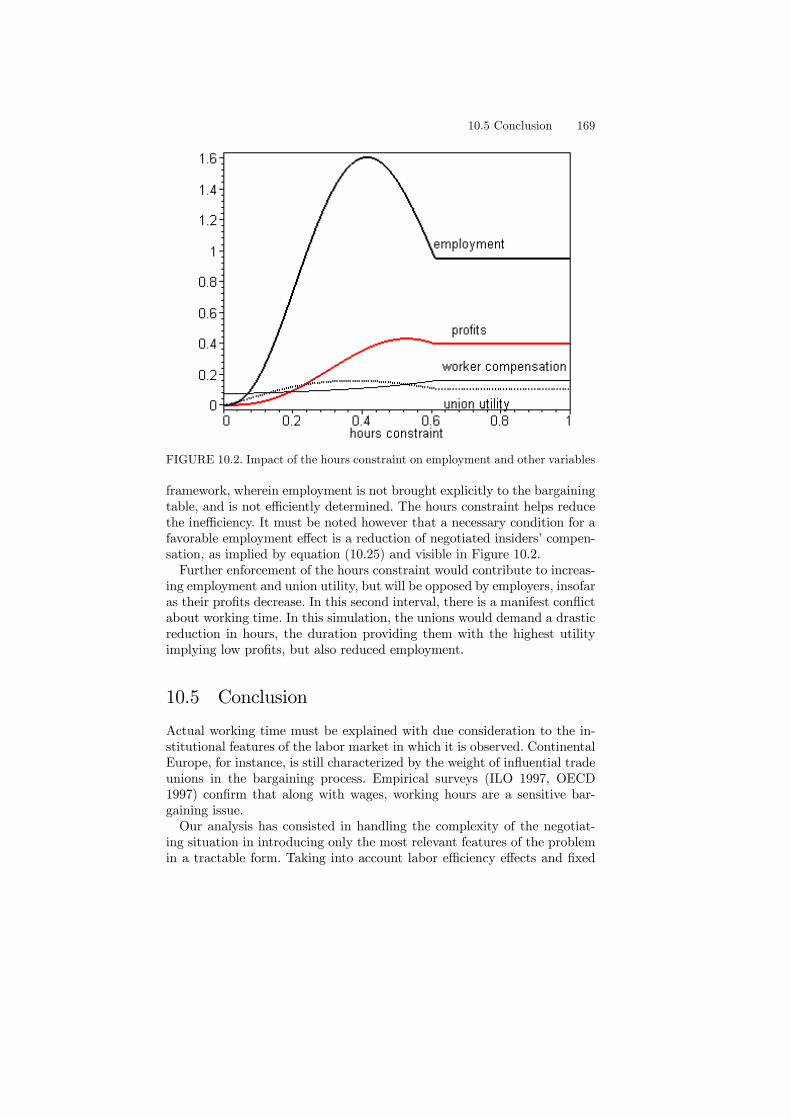
10.5 Conclusion 169
FIGURE 10.2. Impact of the hours constraint on employment and other variables
framework, wherein employment is not brought explicitly to the bargainingtable, and is not efficiently determined. The hours constraint helps reducethe inefficiency. It must be noted however that a necessary condition for afavorable employment effect is a reduction of negotiated insiders’ compen-sation, as implied by equation (10.25) and visible in Figure 10.2.Further enforcement of the hours constraint would contribute to increas-
ing employment and union utility, but will be opposed by employers, insofaras their profits decrease. In this second interval, there is a manifest conflictabout working time. In this simulation, the unions would demand a drasticreduction in hours, the duration providing them with the highest utilityimplying low profits, but also reduced employment.
10.5 Conclusion
Actual working time must be explained with due consideration to the in-stitutional features of the labor market in which it is observed. ContinentalEurope, for instance, is still characterized by the weight of influential tradeunions in the bargaining process. Empirical surveys (ILO 1997, OECD1997) confirm that along with wages, working hours are a sensitive bar-gaining issue.Our analysis has consisted in handling the complexity of the negotiat-
ing situation in introducing only the most relevant features of the problemin a tractable form. Taking into account labor efficiency effects and fixed

170 10. Working time in a trade union model
costs, the model captures the main elements of the profit structure of thefirm. The union has a rather general objective, allowing for variable weightassigned to individual and collective interests. The Nash approach to thenegotiation problem makes it possible to compound the conflicting objec-tives of the parties and to determine employment and the final terms ofthe labor contract.It must be acknowledged, however, that this model cannot claim to be
a full general equilibrium construction and should be seen as a first steptowards a more complete treatment. The fixed costs have been consideredas full dissipation of value. In fact, they represent resources for a secondomitted sector supplying the corresponding services and whose activity isproportional to these costs. While the model fully takes into considerationthe relation between the negotiated variables and the employment level, itdoes not take into consideration the link between employment and the taxburden related to unemployment benefits. Thus, our model is relevant ifnegotiations take place at a highly decentralized level, the union taking asgiven global unemployment; in the opposite case of centralized bargaining,the tax impact on the demand for workers should be brought into thepicture.The analysis in this chapter finally reveals an important structural fea-
ture of the unionized economy, i.e. the relationship between exogenouslyimposed maximum working time and the employment level obtaining whenthe parties have expressed their bargaining powers. By numerical simula-tion, it has been shown that if a limit on the duration of work is imposed onan initially unconstrained system, decentralized negotiation may, at first,induce reduced compensation for the incumbent workers and therefore afavorable effect on employment might be expected. Further enforcement ofthe constraint would entail perverse employment consequences.
10.6 Appendix: Main elasticities and theirrelationships
When working time is predetermined either by legal constraint or by nego-tiated commitments, the demand for workers by the firm eliminates onlythe extensive margin, and the following equations hold:
πN = 0⇔ αAnα−1hαβ = wh+ θ (10.32)
by = F (n, h) = Anαhαβ (10.33)
Multiplying equation (10.32) by n gives αby = wnh + θn = E (labor ex-penses) and therefore profit is related to output by:
bπ = (1− α)by (10.34)

10.6 Appendix: Main elasticities and their relationships 171
Employment elasticities with respect to wages and hoursTaking logarithms of equation (10.32) yields:
ln {αA}+ (α− 1) ln {n}+ αβ ln {h} = ln {wh+ θ} (10.35)
Taking the partial derivative of equation (10.35) with respect to w:
(α− 1)n
∂n
∂w=
h
wh+ θ
and finally:
ηnw = −µ
1
1− α
¶wh
wh+ θ(10.36)
Taking the partial derivative of (10.35) with respect to h:
(α− 1)n
∂n
∂h+
αβ
h=
w
wh+ θ
and multiplying the two sides by h :
ηnh =αβ
1− α−µ
1
1− α
¶wh
wh+ θ(10.37)
Definingαβ
1− α= δ, equation (10.37) and equation (10.36) are related by:
ηnh = δ + ηnw (10.38)
Profit elasticities with respect to wages and hoursProfit elasticities with respect to w and h can be related to ηnw in the
following way:From equation (10.34), ηπw = ηyw and ηπh = ηyh.From equation (10.33), ηyw = αηnw and we can write:
ηπw = αηnw (10.39)
From (10.33), ηyh = αηnh + αβ and therefore:
ηπh = αηnh + αβ (10.40)
To show the relation between ηπh and ηπw, it is possible either directly tocalculate the elasticities at a point where equation (10.32) holds, or equiv-alently to combine equations (10.38), (10.39) and (10.40). The value ofηnh from equation (10.38) is introduced in equation (10.40), giving ηπh =αδ + αηnw + αβ.From equation (10.39), ηnw = α−1ηπw, therefore:
ηπh = δ + ηπw (10.41)

172 10. Working time in a trade union model

This is page 173Printer: Opaque this
11Complementary labor services andworking time regulation
11.1 Introduction
The preceding chapters analyzed how working time is determined in theabsence of hours regulations, then examined the impact of binding hoursconstraints on the main endogenous economic variables, in particular, onthe level of employment. This chapter and the next one will analyze theimpact of a mandatory reduction in working hours on employment un-der more detailed assumptions concerning the structure of the productiveprocess.As mentioned in Chapter 3, the main objective of the working time policy
in periods of high unemployment is to prompt firms to hire more workersand most work-sharing policies finally call for a uniform reduction in theworking day for all activity sectors, qualifications and occupations. Suchsimple forms of the work-sharing paradigm are undoubtedly based on aspecial technological case in which workers are perfect substitutes for oneanother.However, as previously reported in Table 2.6, observable working hours
are the highest for qualified workers and the lowest for the less qualifiedones. For instance, in the European Union, in 1997, managers worked inaverage 43.9 hours a week, while less qualified workers spent only 32.4 hoursa week at the workplace (Eurostat, 1998).A model with globally substitutable labor services could indirectly ac-
count for this stylized and pervasive fact. The elementary neoclassicalmodel detailed in Chapter 4 is able to explain the diversity of work du-

174 11. Complementary labor services and working time regulation
rations, by considering segmented labor markets and differences in pref-erences; yet, such an explanation cannot account for workers’ internal ra-tioning reported in different surveys (Chapter 2). As put forward in otherchapters, the fixed cost of labor and varying effectiveness in time may ex-plain the wedge between the optimal duration of work from the firm’s pointof view and the hours desired by the workers. These models are also basedon the assumption of substitutable labor services.In this chapter, we explore the consequences of the special case in which
two types of work are considered. The two types will be interpreted inrelation to the qualification level. There is perfect substitution within eachtype: an assembly line worker may be replaced by another or a salesmanby another salesman, and perfect complementarity is assumed between thetwo types of labor services. Working time may be set independently for thetwo types. Workers of both groups may have different effectiveness in time,in keeping with the nature of their jobs. It will be seen in particular thatif the effectiveness of the less qualified workers is more affected by fatiguethan it is for the qualified, a shorter working time may be imposed on themby the cost minimizing firms.In this case of basic complementarity between two forms of labor services
related to two types of different workers, a policy of working time reductionactually binding only for the qualified staff may entail quite paradoxical ef-fects. As the unit cost of the labor service increases, the total demand forthose services is depressed; the direct consequence is a reduction in the de-mand for non-qualified workers. This is clearly an undesirable consequence,insofar as the less qualified workers are more exposed to unemploymentthan the qualified. As Table 11.1 shows, this pattern is stable throughoutthe Western world. For instance, in 1995, the EU-15 unemployment rate ofthose having an education level inferior to secondary level is 13.7%, whilethe unemployment rate of those having a university degree is only 5.8%.Below, we present a formal model of working time determination within a
profit-maximization framework, a context that has been analyzed at lengthin Chapter 9, but with two complementary forms of labor services. Westill consider that labor market competition compels firms to design la-bor contracts compatible with the participation constraint, i.e. implying aminimum utility level attainable by workers. After specifying the main as-sumptions, we analyze the decision problem of the firm, then we study theinfluence of an hours constraint on the demand for each type of workers.

11.2 Main assumptions 175
Minimum education level:Lower thansecondary
SecondaryHighereducation
Belgium 13.4 7.5 3.6France 14.0 8.9 6.5Germany 13.3 7.9 4.9Ireland 16.4 7.6 4.2Italy 9.1 7.9 7.3Spain 20.6 18.5 14.5The Netherlands 7.9 4.8 4.1Sweden 10.1 8.7 4.5UK 12.2 7.4 3.7EU-15 13.7 8.2 5.8OECD 12.3 6.5 4.2
TABLE 11.1. Unemployment rate with respect to education level, 1995. Source:OECD, Employment Outlook, 1998.
11.2 Main assumptions
11.2.1 The production function and the structure of laborservices
We consider that the firm uses a homogeneous flow of labor input measuredby L. One unit of this input is obtained by combining one unit of laborservices of type 1 (non-qualified) and λ units of labor services of type 2(qualified). Qualified and less qualified workers are therefore strictly com-plementary. The parameter λ is a fixed ratio related to the applied technol-ogy. The composite labor input may be combined with existing equipmentto produce the final good. For a constant stock of capital, output is aconcave function in the labor input, y = F (L), with F 0 > 0, F 00 < 0.The flow of non-qualified labor services (index 1) is supplied by n1 em-
ployees working h1 hours in terms described by a constant elasticity func-tion: g1(n1, h1) = n1h
β11 ; the flow of qualified labor services (index 2) is
supplied by n2 employees working h2 hours and is indicated by g2(n2, h2) =n2h
β22 .We assume that the working times of qualified and less qualified workers
are set independently. We further assume that, due to exertion, outputelasticity with respect to hours is lower than unity. This fatigue effect isassumed to be stronger in the case of less qualified workers. Formally, 0 <β1 < β2 ≤ 1.

176 11. Complementary labor services and working time regulation
11.2.2 Worker compensating wage
Workers have neoclassical preferences, represented by the utility functionu (wh, 1− h) , where w is the hourly wage rate, and 1 − h is the availableleisure time. As in the previous chapters, the representative firm has toprovide workers with a minimum satisfaction level, denoted by s. The pro-ducers’ constraint is thus u (wh, 1− h) ≥ s, and for well-behaved utilityfunctions, the constraint should be saturated in the labor cost minimiza-tion problem. The compensating wage rate w(h) conditional for the utilityrequirement s is then implicitly defined by: u [hw(h), 1− h] = s.In the case of segmented labor markets for qualified and non-qualified
workers, this minimum utility level might not be the same. In purely com-petitive labor markets, this satisfaction level should be consistent with fullemployment; but our approach is also compatible with positive unemploy-ment if the satisfaction requirement is subject to downward rigidity. Thislast interpretation yields the framework in which work-sharing policies inthe form of working time limits may be analyzed.For simplicity, we introduce an analytically convenient form of utility
function:
u (wh, 1− h) = [wh]γ [1− h](1−γ) (11.1)
where γ ∈ [0, 1]. The resulting compensating wage function is then: w(h) =
s1γ [1− h]
γ−1γ h−1, implying a compensated wage-hours elasticity:
ηwh =hw0(h)
w(h)=
h− γ
γ(1− h)(11.2)
For a predetermined wage rate w, the corresponding Walrasian hours sup-ply is:
hs(w) = argmaxh{u (wh, 1− h)}
It can be verified that with the particular utility function defined in (11.1),hs(w) = γ ∀w.
11.3 The unconstrained hours decision of the firm
The profit function of the firm is π = F (L)−mL, wherem is the cost of oneunit of the composite labor input. On our assumptions, m does not dependon L and profit maximization may be divided for analytical purposes intotwo stages.In the first stage, the cost of the labor input must be minimized. The
cost incurred by the firm for each unit of labor services is the sum of the

11.3 The unconstrained hours decision of the firm 177
costs of the two types of labor services; it takes the form:
m(n1, n2, h1, h2) = n1h1w1(h1) + n2h2w2(h2) (11.3)
where w1(h1) and w2(h2) are the relevant compensating wage functions.1
The first problem consists in determining m = min {m(n1, n2, h1, h2)}, thecontrol variables of the firm being n1, n2, h1, h2. In the second stage, thefirm determines L∗ = argmax
L{F (L)− mL} .
11.3.1 The cost minimization problem
There is no constraint on available workers, but one unit of labor inputrequires one unit of less qualified labor services and λ units of qualified ones;consequently, the constraints n1h
β11 = 1 and n2h
β22 = λ apply. Therefore,
we substitute in (11.3) n1 with h−β11 and n2 with λh
−β22 obtaining a new
form of the objective function with only two independent arguments:
m(h1, h2) = h1−β11 w1(h1) + λh
1−β22 w2(h2) (11.4)
First order conditions are thus:
∂m
∂h1= (1− β1)h
−β11 w1(h1) + h
1−β11 w01(h1) = 0
∂m
∂h2= λ(1− β2)h
−β22 w2(h2) + λh
1−β22 w02(h2) = 0
In terms of the hours-elasticity concept applied to the compensating wagefunctions w(h), the two first order conditions may be written:
ηw1h1 = −(1− β1) (11.5)
ηw2h2 = −(1− β2) (11.6)
But according to equation (11.2), ηw1h1 =h1 − γ1
γ1(1− h1)and ηw2h2 =
h2 − γ2γ2(1− h2)
.
Optimal hours from the firm’s point of view are therefore:
h1 =γ1β1
1− γ1 + γ1β1(11.7)
h2 =γ2β2
1− γ2 + γ2β2(11.8)
1We omit for the purpose of parsimony the fixed costs of labor.

178 11. Complementary labor services and working time regulation
Cost minimizing hours increase in both parameters, i.e. increase when work-ers assign higher importance to consumption or when worker effectivenessdecreases less strongly in the duration of work.
It can be noticed that β < 1 and γ ∈ ]0, 1[⇒ h =βγ
1− γ + γβ< γ = hs,
indicating that rationing prevails: the hours laid down in the labor contractdo not satisfy the individual supply (workers are in a situation of insideunderemployment).In this framework, the longer hours of work of the qualified (type 2) can
be explained by considering the respective values of γ and β for the twotypes. Since h increases in the two parameters, it can be said that for iden-tical consumption/leisure preferences, longer hours are explained by lesstime dependent effectiveness β2 > β1 (due to more significant physical ex-ertion during the working day for type 1). If effectiveness follows the sametime pattern for both types (β1 = β2) longer working time for type 2 isexplained by differences in consumption/leisure preferences: more exhaust-ing and monotonous tasks for the less qualified are expressed by γ1 < γ2,implying h1 < h2.The minimum cost of the labor unit is obtained by introducing in equa-
tion (11.4) the durations indicated by equations (11.7) and (11.8).In the following, in order to keep the analysis as simple as possible, we
only consider the case of identical preferences, γ1 = γ2 = 1/2, and wherethe satisfaction level s is the same in the two markets. The compensated-wage functions are therefore identical and take the special form: w(h) =s2/h(1 − h). In this case, optimal working times are respectively h1 =
β1/(1 + β1) and h2 = β2/(1 + β2), the differences in the effectivenessfunction alone being responsible for the hours wedge.The minimum unit cost is:
m = s2∙(1 + β1)
1+β1
(β1)β1
+ λ(1 + β2)
1+β2
(β2)β2
¸(11.9)
11.3.2 Optimal employment
Then, the total demand for labor input can be obtained by considering theprofit function of the productive sector:
π = F (L)− mL (11.10)
The first order condition is: F 0(L∗) = m, which determines the demandfor labor input L∗ = F 0−1(m). By differentiating this condition, we get thesensitivity of the demand for labor input with respect to cost:
dL∗
dm=
1
F 00(L∗)< 0 (11.11)

11.4 Employment under the hours constraint 179
The demand for non-qualified workers is then: n∗1 = L∗h−β11 , and the de-
mand for qualified workers is: n∗2 = λL∗h−β22 .
Finally, the activity level is F (L∗).
11.4 Employment under the hours constraint
11.4.1 The analytical approach
This model makes it possible to analyze the employment impact of amandatory constraint on working time. If the maximal duration of work islimited by a legal constraint, h ≤ h, two situations may be considered:a) the hours constraint applies only to those workers who perform the
longer hours, i.e. the qualified: h1 < h < h2. Introducing h in the wage-compensating function of type 2 workers yields the new expression for theunit cost:
m(h1, h) = s2∙(1 + β1)
1+β1
(β1)β1
+ λh(−β2)
1− h
¸(11.12)
The unit cost can only increase with reduced hours. In this case, the demandfor total labor input will diminish (dL∗ < 0). As working time of the non-qualified (h1) is unchanged, this implies a reduced demand for this type ofworker (dn∗1 < 0).As to the qualified workers, the cost-increase effect can be offset by a
substitution effect; the total impact on the demand for qualified workers isundetermined.b) the hours constraint applies to both sets of workers: 0 < h < h1. The
unit cost is:
m(h) = s2∙h(−β1)
1− h+ λ
h(−β2)
1− h
¸(11.13)
Two opposing effects are at work: while the unit cost increase entails areduced demand for labor services, the man-hours substitution tends toincrease the demand for workers.
11.4.2 A numerical example
In order to better represent the impact of the hours constraint on thedemand for workers, we will carry out a numerical analysis. We consider thetechnology represented by the production function F (L) = Lα. Parametersare assigned: α = 0.75, λ = 0.5, β1 = 0.5, β2 = 0.85 and s2 = 0.1.Figure 11.1 depicts employment of the non-qualified (n1), Figure 11.2
represents employment of the qualified (n2), and Figure 11.3 representstotal employment n1+n2 (qualified and non-qualified) in the three regions.

180 11. Complementary labor services and working time regulation
FIGURE 11.1. Demand for less qualified workers
FIGURE 11.2. Demand for highly qualified workers
Without constraint (or if the constraint is not binding, h2 < h), theoptimal free durations are h1 = 1/3 and h2 = 0.46. Optimal demand forlabor services is L∗ = 8.52; these services are provided by n∗1 = 14.76non-qualified workers and n∗2 = 8.25 qualified workers.If h1 < h < h2, the unit cost (11.12) increases, L∗ diminishes, h1 = 1/3
is constant, thus n∗1 decreases. On the other hand, n∗2 increases initially
in keeping with a strong man-hours substitution effect. Total employmentincreases, reaches a maximum, then decreases.If 0 < h < h1, the unit cost is given by (11.13). The two opposite effects
are at work, but the effect of reduced demand for labor services dominates.

11.5 Conclusion 181
FIGURE 11.3. Total demand for workers
11.5 Conclusion
Most models of working time determination, including those presented inearlier chapters of this text, are based on a simplifying assumption of homo-geneous workers, substitutable in particular in the supply of labor services.This chapter offers a countervailing example of an economy in which a strictcomplementarity is assumed between two types of labor, made necessary bythe technology currently applied to produce the representative commodity.We have seen that heterogeneous individual preferences and effectivenessin time explain the observed differences in working hours between two com-plementary groups, which may be interpreted as highly qualified and lessqualified workers.When working time limits are superimposed on such a system, it is shown
that the impact of a moderate value of the constraint on working time maybe favorable to global employment. The structure of employment is howevermodified, with the creation of qualified jobs and destruction of non-qualifiedjobs: the policy is not neutral and, unfortunately, would harm those who arethe most exposed to unemployment in the present situation faced by mostcountries in the Western world, i.e. the less qualified workers. Obviously, if

182 11. Complementary labor services and working time regulation
joblessness only affects the non-qualified, such a policy would apply under ashortage of qualified workers; in this case, the adverse effect on unqualifiedjobs would be more significant than suggested by our simulation and wouldbe the only outcome of the mandatory working time reduction.

This is page 183Printer: Opaque this
12Working time reduction in avertically integrated two-sector model
12.1 Introduction
In a context of massive unemployment, a mandatory reduction in work-ing hours is intended to increase the demand for workers and improve thedistribution of rationing in the labor market, more people being neededto supply a constant flow of working hours. In practice, governments havesometimes proved themselves reluctant to impose working hours reductionson industries producing tradable commodities exposed to foreign competi-tion. Some of them have enforced or inspired such constraints in the sectorsmainly producing non-tradable commodities. For instance, in France, thestate-owned company producing and distributing electricity (EDF) adopteda shortened working week by January 1997 (35 hours as compared withthe standard 39 hours) and claimed to alleviate the burden of joblessnessthrough the process of man-hours substitution. A similar working timeconfiguration is reported in Italy. According to CNEL, the Italian nationalcenter for economic and labor research, in 1998, the ENEL state-ownedelectricity monopoly operated under a negotiated 38 hour week, while thepredominant model in the other manufacturing sectors was of 40 hours perweek.In this chapter, we set out to examine in general quantitative terms how
a working time constraint imposed on a first sector producing a factorof production impinges on the total number of jobs supplied in a closedeconomy, when insiders in the job market are able to defend a predeter-mined satisfaction level. The model combines a simple submodel explain-
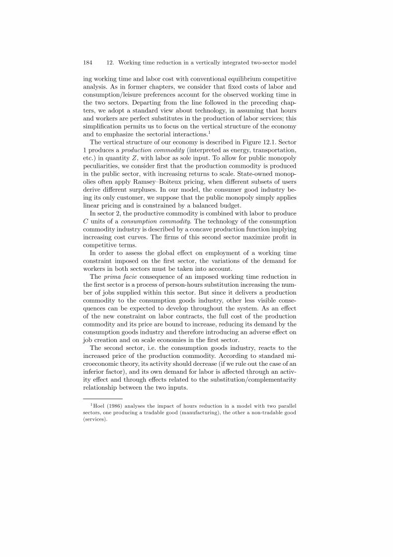
184 12. Working time reduction in a vertically integrated two-sector model
ing working time and labor cost with conventional equilibrium competitiveanalysis. As in former chapters, we consider that fixed costs of labor andconsumption/leisure preferences account for the observed working time inthe two sectors. Departing from the line followed in the preceding chap-ters, we adopt a standard view about technology, in assuming that hoursand workers are perfect substitutes in the production of labor services; thissimplification permits us to focus on the vertical structure of the economyand to emphasize the sectorial interactions.1
The vertical structure of our economy is described in Figure 12.1. Sector1 produces a production commodity (interpreted as energy, transportation,etc.) in quantity Z, with labor as sole input. To allow for public monopolypeculiarities, we consider first that the production commodity is producedin the public sector, with increasing returns to scale. State-owned monop-olies often apply Ramsey—Boiteux pricing, when different subsets of usersderive different surpluses. In our model, the consumer good industry be-ing its only customer, we suppose that the public monopoly simply applieslinear pricing and is constrained by a balanced budget.In sector 2, the productive commodity is combined with labor to produce
C units of a consumption commodity. The technology of the consumptioncommodity industry is described by a concave production function implyingincreasing cost curves. The firms of this second sector maximize profit incompetitive terms.In order to assess the global effect on employment of a working time
constraint imposed on the first sector, the variations of the demand forworkers in both sectors must be taken into account.The prima facie consequence of an imposed working time reduction in
the first sector is a process of person-hours substitution increasing the num-ber of jobs supplied within this sector. But since it delivers a productioncommodity to the consumption goods industry, other less visible conse-quences can be expected to develop throughout the system. As an effectof the new constraint on labor contracts, the full cost of the productioncommodity and its price are bound to increase, reducing its demand by theconsumption goods industry and therefore introducing an adverse effect onjob creation and on scale economies in the first sector.The second sector, i.e. the consumption goods industry, reacts to the
increased price of the production commodity. According to standard mi-croeconomic theory, its activity should decrease (if we rule out the case of aninferior factor), and its own demand for labor is affected through an activ-ity effect and through effects related to the substitution/complementarityrelationship between the two inputs.
1Hoel (1986) analyses the impact of hours reduction in a model with two parallelsectors, one producing a tradable good (manufacturing), the other a non-tradable good(services).

12.2 Explaining working time: a simple model of the labor contract 185
SECTOR 1Productioncommodity Z
SECTOR 2Consumptioncommodity
labor
L1
labor
L2
C Demand
FIGURE 12.1. Vertical structure of the economy
The developments below aim at bringing out the relevant parametersrelated to preferences and technology enabling us to assess the final impactof the suggested constraint on the aggregate job supply in the economy.The validity of the results is limited to small variations of the working timeconstraint; more radical changes would require a different approach takinginto account discontinuities in the labor cost functions.The chapter is organized as follows: the spontaneously adopted working
time in the two sectors is analyzed in the next section. Section 12.3 intro-duces with more precision the structure and decisions of the two sectors.The comparative statics of the model when a working time constraint is im-posed on the first sector is studied in section 12.4. Section 12.5 introducestwo special cases related to fixed proportions; in the second one, sector 1is private and can be interpreted as road transport.
12.2 Explaining working time: a simple model ofthe labor contract
12.2.1 The compensating wage function
Workers have individual consumption/leisure preferences represented bya utility function u(c, l) where c and l represent daily consumption andleisure. This function is assumed to have the standard neoclassical proper-ties. The time unit being the day, the working time h ∈ ]0, 1[ and with alinear real wage rate (in units of the consumption good) w, we can write:
u(c, l) = u(wh, 1− h) (12.1)
The labor supply constraint is represented by a minimum utility level sobtained by the worker. The value of s could be endogenous in a competi-tive labor market and compatible with full employment. We are interested

186 12. Working time reduction in a vertically integrated two-sector model
however in a situation with static unemployment and consider thereforethat union power, insider privileges, or a generous unemployment compen-sation policy explain a level of s non-compatible with labor market staticequilibrium (there is excess supply of workers). Provided that the utilityconstraint is satisfied, the firm determines wages and working time.From equation (12.1), we derive the compensating wage function w(h)
defined by:
u(hw(h), 1− h) = s
As in Chapter 9, we assume preferences such that: w00(h) > 0, ∀h ∈ ]0, 1[ .2
12.2.2 The optimal contract
The techniques applied in the two sectors share the neoclassical propertyaccording to which the labor input L can be measured by the product nh,where n is the number of workers. This means that workers and hours areperfect substitutes (in logarithms) and that our model does not take intoaccount possible productivity effects of the working time variations.The cost of the labor input L is explained by wages and fixed costs
of labor, i.e. costs related to the number of workers n only (described inChapter 5). We consider linear fixed costs of the form θn, implying that,for any labor input L = nh, the labor cost function can be written as:
Ψ(L, h) = w(h)L+ θL
h(12.2)
or, in an equivalent form, Ψ(L, h) = LH(h), with:
H(h) = w(h) +θ
h(12.3)
H(h) represents the full cost of one unit of labor input. Using our assump-tions, it is easily checked that H 00(h) > 0, and first order condition of costminimization explains the optimal working time decided by the firm, h∗:
Ψh(L, h∗) = LH 0(h) = 0⇔ w0(h∗) =
θ
(h∗)2,∀L (12.4)
Some features of the labor cost minimizing contract are worth noticing:— The optimal contract (h∗, w(h∗)) is a separate choice (independent of
the activity level determination and of the demand for L).— As shown in Chapter 9, the fixed cost of labor introduces a systematic
conflict about working time since the optimum value for the firm h∗ is
2As already mentioned, this property is not a general consequence of standard neo-classical assumptions on u(, ) but can be exemplified by very simple utility functionssuch as u = wh(1− h) yielding the compensating wage function w(h) = s/h(1− h).

12.3 The vertical structure of the economy 187
higher than the individual labor supply hs[w(h∗)]. Reduction of workingtime for a constant wage rate would improve the worker’s utility.— If there are two sectors i = (1, 2), the labor market can be considered
either as homogeneous (s1 = s2) or segmented (s1 6= s2). In each sector, itis therefore possible to define Hi(h), the full cost of one unit of labor input,as a function of h, such thatHi(h) = wi(h)+θi/h. On our assumptions, thisfunction admits a unique minimum value h∗i , and hi < h∗i ⇒ H 0
i(hi) < 0and hi > h∗i ⇒ H 0
i(hi) > 0.
12.3 The vertical structure of the economy
The economy comprises two vertically linked sectors. In sector 1, a produc-tive commodity (interpreted as energy, transportation, etc.) is producedin quantity Z, with labor as sole input. In sector 2, the productive com-modity is combined with labor in producing C units of the consumptioncommodity. Sector 2 is the only customer of sector 1.
12.3.1 Sector 1: Production of the productive service.
Technique is described by the production function: Z = F (n1h1) = F (L1).Our increasing returns assumption implies F 00(L1) > 0 and explains publicownership or public control of a single firm. The activity Z of the sector 1is explained by the demand from sector 2.The profit in sector 1 may be written as:
π1 = pF (n1h1)− [w1(h1)n1h1 + θ1n1] (12.5)
where w1(h1) is the compensating wage function associated with a prede-termined utility level s1 and p is the price of the productive commod-ity in terms of the consumption good. In more compact terms: π1 =pF (L1)− L1H1(h1).We assume that the price of the productive commodity or service is set
in application of a zero profit rule:
pF (L1)− L1H1(h1) = 0⇒ p =H1(h1)
q(Z)(12.6)
where q(Z) ≡ F (L1)/L1 is the average productivity of labor in sector 1(q0(Z) > 0).For a given activity Z, the minimum value of p obtains if the labor cost
is minimized by the optimal contract (h∗1, w1(h∗1)) and:
p =w1(h
∗1) + θ1/h
∗1
q(Z)=
H1(h∗1)
q(Z)(12.7)
188 12. Working time reduction in a vertically integrated two-sector model
When a working time constraint h1 is imposed on sector 1, we can writemore generally:
p(Z) =H1(h1)
q(Z)(12.8)
12.3.2 Sector 2: Production of the consumption commodity
The technology applied in this sector is represented by a neoclassical (con-cave) production function relating the number of produced units C to factorconsumption: C = G(L2, Z), where L2 = n2h2.The profit function is:
π2 = G(L2, Z)− w2(h2)L2 − θ2L2h2− pZ (12.9)
where w2(h2) is the compensating wage function associated with a pre-determined utility level s2. Sector 2 is free in determining working time,which will constantly be set at its optimum value h∗2. Therefore:
π2 = G(L2, Z)− L2H2(h∗2)− pZ (12.10)
Profit maximization in sector 2 determines explicitly the demand for laborL2, and implicitly the demand for labor L1, through its demand for Z.The representative firm of sector 2 is a price-taker (takes p as given) andmaximizes its profit.First order conditions applying to maximization of (12.10) are:⎧⎪⎨⎪⎩
∂π2∂L2
= GL (L∗2, Z
∗)−H2(h∗2) = 0
∂π2∂Z
= GZ (L∗2, Z
∗)− p = 0(12.11)
where L∗2 and Z∗ represent the demands for workers and productive services
by sector 1. Obviously, they are both functions of the relative price of theproductive commodity, p.
12.4 Equilibrium and comparative statics
12.4.1 A graphic introduction
First order conditions (12.11) and equation (12.8) determine together theendogenous variables for any value of h1.Graphically (Figure 12.2), the solution can be illustrated in space (OZ,Op)
in which it is possible to draw for a given value of h1:

12.4 Equilibrium and comparative statics 189
— a balanced budget equilibrium locus BB of sector 1, representing p(Z)according to equation (12.8); its negative slope results from our assumptionthat q0(Z) > 0;— a curve representing the demand function for the production good
Z∗(p), denoted by DD. From the general theory of factor demand by com-petitive firms, we know that the slope of this curve is negative. (We considerthe case where the slope of Z∗(p) is steeper than the slope of BB assuming“small” values of q0(Z).)The intersection of the two curves noted (ZE , pE) shows the values of
two endogenous variables in equilibrium.
E
E'
D
D
B
B
B'
B'
0Z
p
price
quantityZE
pE
dh1<0_
FIGURE 12.2. Equilibrium and comparative statics
Comparative statics can be sketched graphically: if we consider an im-posed reduction of working time in the first sector, the labor cost increasesin sector 1 and the BB locus shifts upwards; therefore, dh1 < 0⇒ dpE > 0and dZE < 0. The reduced demand for the productive service introduces afirst offsetting effect on the demand for workers in sector 1.The price variation dpE > 0 entails variations of the activity and of the
demand for labor in sector 2. If the productive factor is not an inferior

190 12. Working time reduction in a vertically integrated two-sector model
factor, the output of the private sector may be expected to diminish. Itsdemand for labor is modified through an activity effect and through asubstitution effect.
12.4.2 The analytical approach
Analytically, we have to determine the local impact of a variation dh onthe total number of available jobs (dN1 + dN2).Equations (12.8) and (12.11) implicitly determine jointly equilibrium val-
ues of a set of principal endogenous variables (Z, p, L2). Since a variation ofp does not change the optimal labor contract in sector 2, a differentiatingsystem (12.11) yields:µ
GLL GLZ
GLZ GZZ
¶µdL2dZ
¶=
µ0dp
Defining D = detµ
GLL GLZ
GLZ GZZ
¶> 0, we can write:
µdL2dZ
¶=1
D
µGZZ −GLZ
−GLZ GLL
¶µ0dp
¶(12.12)
thus:
dL2 = −GLZ
Ddp (12.13)
dZ =GLL
Ddp (12.14)
Differentiating equation (12.8), we obtain:
q(Z)dp+ pq0(Z)dZ = H 01(h1)dh1 (12.15)
Substituting (12.14) for dZ in (12.15), we obtain the sensitivity of theequilibrium value of p with respect to h1:
dp
dh1=
DH 01(h1)
Dq(Z) + pq0(Z)GLL(12.16)
From (12.13) and (12.16), we obtain the sensitivity of the equilibrium valueof L2 with respect to h1:
dL2dh1
= − GLZH01(h1)
Dq(Z) + pq0(Z)GLL(12.17)
Finally, (12.14) and (12.16) imply:
dZ
dh1=
GLLH01(h1)
Dq(Z) + pq0(Z)GLL(12.18)

12.4 Equilibrium and comparative statics 191
The sign of the different sensitivities is ambiguous in the general case. Wemust notice that if the working time is initially free in the first sector(h1 = h∗1), we know from (12.4) that H
01(h1) = w01(h1)−θ1/h21 = 0 and the
numerator of the three last equations is nil in the first order. For h1 < h∗1however, i.e. if the working time is already suboptimal from the firm’s pointof view, H 0
1(h1) < 0.The sign of the denominator Dq(Z)+pq0(Z)GLL is clearly related to the
differences of the slopes (Figure 12.2) of the locus BB and of the demand
curve Z∗(p) for the productive good. The first slope isµdp
dZ
¶BB
= −pq0(Z)
q(Z)
and the slope of the demand curve is (from 12.14)µdp
dZ
¶DD
=D
GLLand
since GLL < 0,D
GLL< −pq
0(Z)
q(Z)⇒ Dq(Z) + pq0(Z)GLL > 0. We consider
in the following that the order of magnitude of scale economies is such thatthe denominator can be considered as positive. In this case, dp > dh1 < 0,dZ/dh1 > 0 and the sign of dL2/dh1 is the same as the sign of GLZ ≷ 0.The final impact of the working time constraint on the total number
of available jobs is obtained by considering the sign and value of (dn1 +dn2)/dh1.In the first sector, we have Z = F (n1h1) and therefore:
dn1dh1
=1
h1F 0(L1)
dZ
dh1− n1
h1
or in elasticity terms:
ηn1h1= −1 +
ηZh1
ηZL1
The first term can be interpreted as representing the “substitution effect”between workers and hours of the constraint variation, the second termbeing the “activity effect”.In sector 2, the working time is constant and therefore:
dn2dh1
=1
h∗2
dL2dh1
The sensitivity of the total number of jobs with respect to the working timeconstraint is explained by three additive terms:
dn1 + dn2dh1
= −n1h1+
1
h1F 0(L1)
dZ
dh1+1
h∗2
dL2dh1
(12.19)
On our assumptions, the favorable substitution effect might be partiallyoffset or more than offset by two other effects. The worst case would take

192 12. Working time reduction in a vertically integrated two-sector model
place when GLZ > 0 since GLZ > 0⇒ dL2/dh1 > 0; reducing the workingtime in sector 1 implies job destruction in sector 2.Values of dL2/dh1 and dZ/dh1 being taken from (12.17) and (12.18), we
can write as a final form:
dn1 + dn2dh1
= −n1h1+
H 01
Dq(Z) + pq0(Z)GLL
∙GLL
h1F 0(L1)− GLZ
h∗2
¸(12.20)
where H 0 < 0, GLL < 0, GLZ ≶ 0.For sufficiently small values of q0(Z) or GLL, the second term of the
right hand side of equation (12.20) is positive iff GLZ >h∗2GLL
h1F 0(L1)(a
negative number). We have to keep in mind that any technology in whichthe marginal productivity of labor is increasing with the consumption ofthe productive commodity implies GLZ > 0 and therefore satisfies thiscondition.
12.5 Special cases of fixed proportions
Our former representation allows for technical substitution between laborand the productive commodity in sector 2. We suggest considering here-after two different special cases of complementarity: in the first case, theproduction commodity is used in a fixed proportion α of labor, Z = αL2(perfect complementarity between the two inputs); in the second case, theproduction commodity is used in a fixed proportion of output, Z = γC.This second case applies in particular when the sector 1 commodity is in-terpreted as a transport service from a predetermined production place toa predetermined consumption area. In both cases, the technology of sector2 is represented by a neoclassical function of a single variable
C = G(L2)
12.5.1 Fixed proportion of labor
In this case, Z = αL2, and the profit function of sector 2 is:
π2 = G(L2)−H2(h∗2)L2 − αpL2
The first order condition is:
dπ2dL2
= G0(L2)− [H2(h∗2) + αp] = 0 (12.21)
Differentiating (12.21) yields
dL2dp
=α
G00(L2)(12.22)

12.5 Special cases of fixed proportions 193
and
dZ
dp=
dZ
dL2
dL2dp
=α2
G00(L2)(12.23)
Using (12.16), we obtain the sensitivities
dL2dh1
=αH 0(h1)
q(Z)G00(L2) + α2pq0(Z)(12.24)
dZ
dh1=
α2H 0(h1)
q(Z)G00(L2) + α2pq0(Z)(12.25)
The sensitivity of the total amount of jobs available (dn1 + dn2)/dh1 isobtained by substituting dL2/dh1 and dZ/dh1 in (12.19) with the righthand side of (12.24) and (12.25).We obtain the following final form:
(dn1 + dn2)
dh1= −n1
h1+
αH 0(h1)
q(Z)G00(L2) + α2pq0(Z)
∙α
h1F 0(L1)+1
h∗2
¸(12.26)
For “small” values of q0(Z), the sign of the second term in (12.26) is positive.Two effects offset the man-hours substitution in sector 1; if G00(L2) alsotakes small values, the order of magnitude of this second term might explainthe overall job destruction when h1 is reduced.
12.5.2 Fixed proportion of output: the trucking case
In France, the threat of strikes and traffic blockades has imposed on firmsa reduced working time in the service activity of road transport (November1997). The model may shed some light on the employment impact of thismeasure.If we interpret sector 1 as supplying transport services to the consump-
tion goods industry, we cannot keep a natural monopoly assumption; weconsider sector 1 as private, working with constant productivity q(Z) = qand under a competitive zero-profit equilibrium. In this case, the BB locusin Figure 12.2 is horizontal and equation (12.8) takes the form:
p =H1(h1)
q(12.27)
As mentioned, the production function indicates C = G(L2). The demandfor the productive factor is Z = γG(L2). The profit function becomes:
π2 = G(L2)−H2(h∗2)L2 − γpG(L2)

194 12. Working time reduction in a vertically integrated two-sector model
where γ is related to the average mileage of the output and p is a per-unitflat tariff.The first order condition is:
G0(L2)(1− γp)−H2(h∗2) = 0 (12.28)
Differentiating (12.27) and (12.28) yields:
dL2dh1
=γG0(L2)H
01(h1)
qG00(L2)(1− γp)(12.29)
and
dZ
dh1=[γG0(L2)]
2H 01(h1)
qG00(L2)(1− γp)(12.30)
The sensitivity of the total amount of available jobs (dn1 + dn2)/dh1 isagain obtained by substituting dL2/dh1 and dZ/dh1 in (12.19) with theright hand side of (12.29) and (12.30). The final form in this special caseis:
dn1 + dn2dh1
= −n1h1+
γG0(L2)H01(h1)
qG00(L2)(1− γp)
∙γG0(L2)
h1F 0(L1)+1
h∗2
¸(12.31)
The sign of the second term of (12.31) is positive (γp < 1). For small valuesof G00(L2), working time reduction in the transport sector may imply jobdestruction at an aggregate level.
12.6 Conclusion
The suggested model is able to indicate the structural elements of the econ-omy accounting for unsatisfactory or paradoxical variations in the numberof available jobs, when working time constraints are applied to the sectorssupplying productive factors or services, and when the workers (insiders)are generally able to defend a constant utility level.In many cases, the perverse effects are negligible if the system is initially
free, i.e. if the working time coincides with its optimum value from thefirms’ point of view, but can play a major role when firms are alreadyconstrained (working time of the truck drivers is obviously constrained bysafety regulations).It must be noticed, however, that joblessness may push down the min-
imum utility requirement. In this case the perverse effect of the appliedworking time constraint would be partially offset by lower compensatingwages. But working time reductions usually seem to be linked to openingnew negotiation rounds between unions and firms. Quite often, the result-ing wage rate variations in the public monopoly do not follow the terms of

12.6 Conclusion 195
a compensatory wage function but improve the utility level of the insiders,sometimes stimulating similar claims in the other sectors.3 In such a case,the total impact on job supply variations is worse than indicated by theterms of our model.
3The French EDF agreement on the reduction of the working week from 38 to 32hours reached in January 1997 is estimated to imply a 9% increase of the hourly wagerate.

196 12. Working time reduction in a vertically integrated two-sector model

This is page 197Printer: Opaque this
13Working hours and unemployment ina matching model
13.1 Introduction
Previous chapters provided several analyses of working time under vari-ous assumptions pertaining to the institutional set-up and the constraintsimposed upon profit maximizing firms of the productive sector. They areall based on a static framework, firms and workers taking once and for alldecisions concerning only one period. This simplifying design allowed us toemphasize the role played by fixed costs of labor and worker time effective-ness functions on the optimal duration of work, given various organizationalcontexts.Recent advances in unemployment analysis build on a dynamic approach
grounded in equilibrium search theory (see the survey by Mortensen andPissarides, 1999). Some authors had provided founding contributions to thisapproach. One should mention the pioneering texts by Stigler (1961), Mc-Call (1970) and various texts collected in a famous book edited by Phelps(1970). More recently, Dale Mortensen and Christopher Pissarides devel-oped this innovative approach in a significant way. These two authors in-troduced a macroeconomic notion of matching technology, explaining howall the firms are able at each point in time to convert vacancies into em-ployment at a rate depending on an indicator of labor market tightness.The standard search economy is subject to a sequence of exogenous
shocks, entailing job destructions and job creations; there are large flowsin and out of jobs, with unemployed persons searching for jobs and firmssearching for workers. In search economies, the influence of costly infor-

198 13. Working hours and unemployment in a matching model
mation technology interfering with decentralized transactions in the labormarket is explicitly modeled. Costly information explains why at any pointin time, unemployed able workers and job vacancies coexist.In this context, Walrasian equilibrium is substituted by search equilib-
rium. As clearly stated by Pissarides (1990, p.4):
Equilibrium in the system is defined by a state in whichfirms and workers maximize their respective objective functions,subject to the matching and separation technologies, and inwhich the flow of workers into unemployment is equal to theflow of workers out of unemployment.
This chapter develops an introductory analysis of working time along thisresearch path. This particular issue was extensively studied by Marimonand Zilibotti (1999) who analyzed the employment impact of a workinghours constraint under various specifications of individual preferences andRocheteau (1999) who worked out a matching model with moral hazard,carrying a step further the “shirking” approach once pioneered by Shapiroand Stiglitz (1984) and applied to the working time issue by Moselle (1996).We focus on the employment behavior of an economy made up of manyfirms, each of them taking the global state of vacancies and unemploymentvariables as given. In contrast to Marimon and Zilibotti (1999) who con-sider homogeneous labor services estimated by the men-hours product, orto Rocheteau (1999) who introduces a technology where output is linearin the number of workers, the generalized production function introducedin this text allows for different output elasticities with respect to hoursand workers. Indeed, as mentioned in Chapter 5, many empirical studieshave shown that hours and workers are not perfect substitutes (in loga-rithms) in the production of labor services. Our approach simplifies on thenegotiation issues (developed in Chapter 10) and plainly considers a partic-ipation constraint expressed with the help of a working time compensatingconsumption function used in an intertemporal framework.The first part of the chapter studies an unregulated labor market, where
the firm is free to choose working time and employment so as to maxi-mize intertemporal profits. We show that the steady state of this economyis fully described by three equations: the obtained system may be numeri-cally solved for the relevant endogenous variables, i.e. hours of work, unem-ployment and probability of filling a vacancy. We put forward a solution inwhich unemployment and individual overwork coexist, an economic contextwhich makes a policy of working time reduction particularly appealingIn the second part of the text, the model is used to study the unem-
ployment effect of a binding constraint on working hours demanded by thefirm. Numerical simulations show that a weak constraint may help to re-duce unemployment down to a minimum value, but further enforcements ofthe constraint entail perverse effects. Particular focus is given to the specialcase where the hours constraint matches the worker supply.
13.2 Main assumptions 199
13.2 Main assumptions
13.2.1 The firm and its technology
The productive sector is represented by a firm producing a homogeneousgood to be sold at a predetermined unit price. Technology is summarizedby a production function having as arguments the number of workers Nand the daily hours per worker h:
F (N,h) = ANαhβ , with: 0 < α < 1, 0 < β,A > 0 (13.1)
Such a function is compatible with different output elasticities with respectto hours and to workers, an empirical finding first put forward by theempirical studies mentioned in Chapter 5. For purpose of parsimony, A = 1.Setting the day as the relevant time period, and using the time index t,daily output is: yt = Nα
t hβt .
All the firms are identical and the number of firms is supposed constant;1
Nt stands simultaneously for the firm’s employment input and for globalemployment.The total labor force is assumed to be constant and equal to L. Therefore
global unemployment Ut = L−Nt.
13.2.2 Workers’ consent to work and the labor contract
Firms retain workers with labor contracts indicating an hourly wage ratewt and the daily hours of work ht. The daily satisfaction of an employedperson (or worker) increases with his consumption possibilities, which arethemselves equal to the daily wage income ct = wtht, and decreases withhours of work, ht. Formally, worker daily satisfaction is of the form S(ct, ht),where t is the day index, with S1 > 0, S2 < 0. The daily satisfaction of theunemployed person is constant and will be denoted S.2
Individuals would accept a contract {wt, ht} if it provides them with anintertemporal utility level (denoted V E) at least equal to the intertempo-ral utility of the unemployed person (denoted V U ). Such a participationconstraint ties the hands of the firms, which must offer workers labor con-tracts such that V E ≥ V U . In this elementary framework, the individualworker has no bargaining power and the employer is able to submit take-itor leave-it contracts.3
1 If f is the number of firms, global employment should be denoted fNt.2This minimal satisfaction index may be written as S = S(b, 1), where b stands for
unemployment benefits. Obviously, ∂S/∂b > 0.3 In Marimon and Zilibotti (1999) or Rocheteau (1999), workers and the firm split
the surplus from the match under a Nash bargaining procedure.

200 13. Working hours and unemployment in a matching model
Proposition 13 The firm should provide workers with a wage compensa-tion such that the daily satisfaction of the employed person equals the dailysatisfaction of the unemployed S(ct, ht) = S.
Proof. Let us denote by q the probability of an employed person losinghis job during the time period t, and by p the probability of an unemployedperson finding a job during the period t. Given a psychological discount rateρ > 0, the expected life-time utility of the employed person is:
V E = S(ct, ht) + (1 + ρ)−1[qV U + (1− q)V E ]
and the expected life-time utility of the unemployed person is:
V U = S + (1 + ρ)−1[pV E + (1− p)V U ]
In an equivalent form, these two equations can be written as:
ρV E = (1 + ρ)S(ct, ht) + q(V U − V E) (13.2)
ρV U = (1 + ρ)S + p(V E − V U ) (13.3)
Substracting (13.3) from (13.2), we get:
(ρ+ q + p)(V E − V U ) = (1 + ρ)[S(ct, ht)− S]
If the firm fixes wages such that V E = V U , then S(ct, ht) = SThe intertemporal decision is thus reduced to the static case studied in
preceding chapters where individuals would accept the terms of the contractif it provides them with a daily (or instantaneous) satisfaction equal to thedaily satisfaction of the unemployed person.Thus c(ht), the minimal daily compensation required by the person asked
to work ht hours, is implicitly defined by:
S(c(ht), ht) = S (13.4)
Notice that c(ht) is one particular indifference curve; it is therefore a convexfunction, in keeping with the standard neoclassical axioms on consump-tion/leisure preferences.For instance, a particular utility function, able to convey in a straight-
forward way the neoclassical assumptions is:
S(ct, ht) = cϕt (1− ht)1−ϕ, ϕ ∈]0, 1[ (13.5)
where the length of the day has been set to one. It implies the compensationfunction:
c(ht) =¡St¢ 1ϕ (1− ht)
ϕ−1ϕ (13.6)

13.2 Main assumptions 201
and a positive compensation-hours elasticity: ηc(h)h =htdc(ht)
c(ht)dht=(1− ϕ)ht(1− ht)ϕ
.
It can be noticed that this elasticity increases in ht.Let us also introduce the concept of individual hours supply, i.e. worker
desired daily hours for any wage rate, hst (wt). Formally, the hours supplyis defined by:
hst = argmaxht
S(wtht, ht) ∀wt (13.7)
Under the former definition of c(h), actual hours coincide with the indi-vidual supply if c0(h) = c(h)/h or ηc(h)h = 1; overwork occurs if c0(h) >
c(h)/h or ηc(h)h > 1.With the particular utility function indicated by equa-tion (13.5), hst = ϕ,∀w.
13.2.3 The matching function
In an economy with decentralized trade, vacant jobs and unemployed jobseekers take time to locate each other; information on vacant jobs is notimmediately available to workers. Thus unemployed persons and vacan-cies coexist and only a fraction of the potential matches occurs during agiven time period. Following the approach pioneered by Diamond (1982),Mortensen (1982) and Pissarides (1984), this complex process may be de-scribed by an aggregate matching function.4
Let us denote by Ut the number of unemployed persons and by Vt thenumber of vacancies. Also, letMt denote the number of unemployed personswho find jobs during period t (i.e. the number of successful matches betweenvacancies and the unemployed). Given the frictions in the labor market,Mt < min{Ut,Vt}. It is further assumed that Mt is an increasing functionin both Vt and Ut, and is quasi-concave and homogeneous of degree one(Pissarides, 1990). It follows that:
Mt =M(Vt, Ut) (13.8)
A convenient form for M(, ) is the constant elasticity specification: Mt =V 1−zt Uz
t , with z < 1.Denoting the relative number of traders in the market by ζt = Vt/Ut,
the probability of filling a vacancy is:
m(ζt) =M(Vt, Ut)
Vt=
V 1−zt Uz
t
Vt=
µVtUt
¶−z= (ζt)
−z (13.9)
4The main innovation of these papers consists in modelling market frictions by an ex-ogenously given matching function relating the number of successful matches per periodto the stock of vacancies and unemployed persons. There is an obvious likeness betweenthe matching technology and a traditional production function which encompasses in asimple relationship the influence on output of two inputs.

202 13. Working hours and unemployment in a matching model
In keeping with traditional literature, ζ = V/U will be interpreted as aproxy for the “tightness” of the labor market.Under these assumptions, the probability of an unemployed person finding
a job during the period t is:
Mt
Ut=
VtUt
Mt
Vt= ζtm(ζt) (13.10)
In the constant elasticity formulation of the matching function, ζtm(ζt) =(ζt)
1−z, thus the probability of finding a job is increasing in ζt.
13.3 The free profit maximization
13.3.1 Profit function and the optimal decision
During each t period, a fraction q of the occupied jobs is destroyed asa consequence of various random shocks that disturb this economy. Thisseparation rate is assumed to be structural. With previous notation, em-ployment evolves according to:
Nt+1 = (1− q)Nt +mtVt (13.11)
where mt = m(ζt). The number of vacancies can thus be written as: Vt =[Nt+1 − (1− q)Nt]/mt.Let κ be the cost of maintaining one vacancy unoccupied. This can be
seen either as an advertising cost or an opportunity cost related to idle cap-ital. Firms also incur fixed costs of labor, proportional only to the numberof employees and which have already been introduced in former chapters.These fixed costs per worker will be denoted by θ. Introducing a discountfactor δ = (1+r)−1, the firm’s objective consists in maximizing the presentvalue P of a sequence of profits:
P =∞Xt=0
δt[Nαt h
βt −Ntc(ht)− θNt − κVt]
=∞Xt=0
δt∙Nαt h
βt −Ntc(ht)− θNt − κ
Nt+1 − (1− q)Nt
mt(13.12)
The firm controls vacancies and hours; employment is indirectly controlledfollowing (13.11). In terms of employment and hours, first order conditionsare:
∂P∂Nt
= 0⇒ αNα−1t hβt = c(ht) + θ +
κ
δmt−1− κ(1− q)
mt(13.13)
∂P∂ht
= 0⇒ βNα−1t hβ−1t = c0(ht) (13.14)

13.3 The free profit maximization 203
In free equilibrium, the firm simultaneously adjusts vacancies (employment)and hours so as to maximize intertemporal profits. The steady state equi-librium may be characterized by three equations.
13.3.2 Three basic equations
The m− h relationship
Let us first substitute Nα−1t = c0(ht)/βh
β−1t in equation (13.13):
αhtc0(ht)
β= c(ht) + θ +
κ
δmt−1− κ(1− q)
mt(13.15)
Denotingα
β= , with ηch =
htc0(ht)
c(ht)and 1/δ = 1 + r, then acknowledging
that in the steady state m(ζt) = m(ζt−1) = m(ζ), the former equationbecomes:
m(ζ) =κ(q + r)
( ηch − 1)c(ht)− θ(13.16)
With the constant elasticity form of the matching function, m(ζ) = (ζ)−z,
z < 1; then (ζt)−z =
κ(q + r)
(kηch − 1)c(ht)− θ, and the probability of getting out
of the unemployment pool is an increasing function of the hours of work:
ζm(ζ) =
∙( ηch − 1)c(ht)− θ
κ(q + r)
¸1− z
z (13.17)
The u− h relationship
Condition (13.14) allows us to infer a relationship between hours and unem-ployment. Indeed, Nα−1
t = β−1h1−βt c0(ht). But for a constant labor force,Nt = L− Ut, it results that:
[L(1− ut)]α−1
= β−1h1−βt c0(ht) (13.18)
where ut = Ut/L is the unemployment rate. In the following, we considerthe case in which due to exertion effect, β < 1, the right hand side of(13.18) is therefore an increasing function in ht, thus the unemploymentrate and hours are positively related.
The u−m relationship
Unemployment dynamics are indicated by:
Ut+1 = Ut + qNt −Mt (13.19)

204 13. Working hours and unemployment in a matching model
As in the steady state Ut+1 = Ut, then qN =M, i.e.: q(L− U) = ζm(ζ)U.After some calculus, we reach the well-known equation:
u =q
q + ζm(ζ)(13.20)
In equation (13.20), the term ζm(ζ) measures the probability of findinga job for an unemployed worker. In the steady state, unemployment is adecreasing function in this probability (itself increasing in ζ). Expressingζm(ζ) in terms of the unemployment rate u and the vacancy rate v wouldyield a Beveridge curve, i.e. a decreasing relationship between the two vari-ables, such as revealed from data by the British economist in the forties.
13.3.3 Equilibrium unemployment and hours of work
Equations (13.16), (13.18) and (13.20) characterize a system with the un-knowns h, u and ζm(ζ). As we consider only steady state values, the sub-script t may be omitted. The solution of the system, if it exists, is denoted{h∗, u∗, ζ∗m(ζ∗)}.
Graphic solution
Figure 13.1 sketches a graphic solution in the plane (Oh,Ou). First, therelationship (13.18) is depicted as the increasing ZZ0 curve. Then, accord-ing to equation (13.20), unemployment decreases in ζm(ζ), the probabilityof the unemployed person finding a job; this probability itself increaseswith working hours in keeping with equation (13.17); we may thereforedraw a second decreasing curve Y Y 0 summarizing the two relationships.The steady state equilibrium is depicted at point E, and characterizes thesteady state equilibrium values of unemployment and duration of work.
Comparative statics of the solution may be performed. For instance, in-creases in q, interpreted as higher economic turbulences, would shift thecurve Y Y 0 upward: hours of work and unemployment increase simultane-ously. Increases in fixed costs θ and κ would have a similar effect.
Numerical solution
The system (13.16), (13.18) and (13.20) may be numerically solved. Weassign a standard figure for α = 0.64; if an exertion effect is at work, onemay reasonably assume that β < α ≤ 1, we thus set β = 0.60. The otherparameters are S = 0.4, ϕ = 0.65, z = 0.25, κ = 0.25, θ = 0.05, r = 0.06,q = 0.15, L = 1. The solution is
h∗ = 0.68
u∗ = 18.45%
ζ∗m(ζ∗) = 0.66

13.4 The policy of working time reduction 205
E
unemployment
hours
Z
Z'Y
Y'
0
FIGURE 13.1. Steady state equilibrium
The daily compensation is equal to c∗ = 0.45 and the firm’s daily profitsare positive, π∗ = 0.169.Notice that a reduction in the minimal satisfaction requirement would
lead — as expected — to a lower unemployment rate (for instance, if S =0.395, u∗ = 16.10%). The impact of other changes in the parameter valuesmay be analyzed in a similar way.Finally, it can be seen that workers are in a situation of overwork, that
is actual working time (h∗) exceeds their hours supply (hs = 0.65).
13.4 The policy of working time reduction
13.4.1 The steady state solutions
The former section developed a simple model of working time and unem-ployment determination in a decentralized economy where the employer isfree to choose the optimal mix of hours and workers. In a context of massiveunemployment, a government may be tempted to impose a constraint onhours of work in order to push firms to substitute hours with workers. Letus denote by h the hours constraint.Under this constraint the firm operates with a positive intensive margin
∂P/∂ht > 0, but is still able to optimize employment: the extensive marginis nil, ∂P/∂Nt = 0 whatever t. Remember that in order to attract workers,the firm must pay them a compensation c(ht).With h = h, two basic equations characterize this economy. The first is
based on the zero extensive margin condition (13.13), ∂P/∂Nt = 0:
αNα−1t hβt = c(ht) + θ +
κ
δmt−1− κ(1− q)
mt(13.21)

206 13. Working hours and unemployment in a matching model
which in the steady state becomes:
αNα−1hβ = c(h) + θ +κ(r + q)
m(ζ)
Given that N = L(1− u), it can alternatively be written as:
α [L(1− u)]α−1
hβ = c(h) + θ +κ(r + q)
m(ζ)(13.22)
The second equation is (13.19), which in the steady state was written as:
u =q
q + ζm(ζ)(13.23)
Equations (13.22) and (13.23) have as a solution the constrained hoursunemployment rate u(h) and the constrained hours probability of obtaininga job, ζm(ζ).Figure 13.2 is the plot of u(h), the steady state unemployment value as
a function of the hours constraint (dark line) against the free equilibriumunemployment u∗ determined in the previous section (grey line). Param-eters were assigned the same values as before while h is allowed to varybetween the upper limit h∗ and an arbitrarily chosen inferior limit.Of course, u(h∗) = u∗. It can be seen in Figure 13.2 that a first favorable
effect appears for an hours constraint in the neighborhood of the optimaltime from the firm point of view (h∗). There exists a duration of workfor which unemployment reaches a minimum. Further enforcements of theconstraint would only increase unemployment.
While the former model is consistent with different working time configu-rations, realistic policy proposals would consider only situations where thehours constraint contributes to reducing overwork. Indeed, a policy aimingat bringing working time below the desired hours from the workers’ pointof view (h < hs) would meet little political support, even if it would furtherreduce unemployment.Given this remark, the most appealing policy in our numerical example
would to be h = hs. Unemployment is u(h = hs) = 16.6% (1.8% less thanin the unconstrained equilibrium), the probability of getting job increasesto ζm(ζ) = 0.7537, daily compensation is c1 = 0.43 and firms’ daily profitsare π1 = 0.1475 (lower than in the unconstrained case).
13.4.2 The adjustment dynamics
In the simulation above, we show that by imposing a constraint on workingtime, the steady state unemployment rate may be reduced. What can besaid about the dynamics of the adjustment?

13.4 The policy of working time reduction 207
h*hs
u(h)
u*
unemployment rate
_
h_
FIGURE 13.2. Steady state unemployment, constrained and unconstrained hours
To answer this question, it should be noticed that after a shock, firmsmay adjust vacancies immediately, while employment and unemploymentwill adjust only gradually. By inspection of equation (13.21), it can beobserved that the variable ζt is “forward looking”, i.e. the tension in thelabor market at date t depends on the tension in the labor market at datet+ 1. Furthermore, there is only one constant value of ζ consistent with afinite expectation of ζt+T when T →∞.5 In this case, after a shock on h, ζwill instantaneously jump to its new steady state value ζ (such as resultingfrom (13.22) and (13.23)), and equation (13.19) alone can characterize theunemployment time path.More precisely, equation (13.19) can alternatively be written as:
ut+1 = ut + q(1− ut)− utζm(ζ)
or
ut+1 = ut[1− q − ζm(ζ)] + q (13.24)
Let us denote u0 the initial unemployment value and [1− q − ζm(ζ)] = a.Then, the unemployment time path is obtained by solving the recursive
5Cahuc and Zylberberg (1996, chapter 7.3.1) provide the formal proof for a relatedproblem.

208 13. Working hours and unemployment in a matching model
equation (13.24). The solution is:
ut = u0at +
1− at
1− aq (13.25)
As |a| < 1, the steady state value of unemployment is finite and equal to:
u(h) = limt→∞
ut =q
q + ζm(ζ)(13.26)
This solution also applies to the particular case provided by the numeri-cal simulation. Initially, unconstrained hours unemployment is u0 = u∗ =18.44. For a constraint, h = hs, the steady state unemployment is broughtdown to 16.60%. Immediately after the shock, unemployment becomes:u1 = au∗ + q = u∗[1− q − ζm(ζ)] + q = 16.77%, the rest of the unemploy-ment reduction taking some more time to occur.
13.5 Conclusion
This chapter builds on a simple matching model à la Pissarides (1990)to analyze how unemployment and working time are determined in a de-centralized labor market with trading frictions. The first part of the textinvestigates a free system, where employers hold the right to manage work-ing time. It is shown that, in some cases, overwork and unemployment mayunfortunately coexist. No doubt, in such an economic context a policy ofworking time reduction may be intuitively appealing.In the second part, the matching model is used to study the macroeco-
nomic impact of a mandatory reduction in working hours. It is shown thatin the neighborhood of the optimal duration from the firm’s point of view,the hours constraint may help diminish the unemployment rate (at theexpense of firm profits); in particular, unemployment is reduced when thehours constraint is equal to the individual supply. The numerical simulationalso shows that there is a working time for which unemployment reachesa minimum; below this threshold, further enforcements of the constraintbring about an increase in unemployment.It must be noticed that introducing the flow vision of the labor market
and the matching problem has not drastically changed the results of sim-ulated working time constraints, as compared to already exposed resultsderived from the static models of previous chapters. The generalized modelobtained with this more accurate representation of labor markets makespossible a better interpretation of the impact of working time policy. Itmust be kept in mind however that model tractability depends upon somesupplementary assumptions, like a predetermined quit rate and indepen-dence of the matching function with respect to endogenous state variables.Simulations tend to show that the existence of consistent solutions of suchmodels is critically confined to a narrow range of the parameter values.

This is page 209Printer: Opaque this
14Deregulation of overtime premiumand employment dynamics
14.1 Introductory concepts: overtime and flexibility
Static cost structure of labor services in relation to working time has beenmainly influenced for years by public regulation, since in most industrialcountries, strict overtime premium rules have prevailed. The Fair LaborStandard Act fixing the determination of overtime premium rates is a sim-ple and typical example of such legal interference. The consequences ofmandatory overtime premium rules have been examined in comparativestatics in Chapter 8.In recent years, however, the role of legal constraints and of legally pre-
determined working time premium rates is tending to recede. In many in-stances, firms are granted more flexibility in adjusting their working hoursto a changing environment. In many countries (to mention only France,Germany, Japan), the trend is in favor of so-called flexibility accords, asindicated in Bosch (1997), Takagi (1993), OECD (1998). Such collectiveagreements may take varied and complicated forms, including a whole set ofcontingent provisions related to various states of the world. However, theyalways embody in some form the terms of a trade-off negotiated betweenthe employers’ need for flexibility and the workers’ preferences for somecentral values of working hours. The compensation of workers is usuallycommensurate with the whole working time profile over the year. This formof collective contract between employers and workers is clearly intended togive more leeway to working time fluctuations than the traditional legalframework.
210 14. Deregulation of overtime premium and employment dynamics
But relaxing legal constraints on the duration of the working week or theworking day does not mean that labor costs become flat in working time.In its attempt to change hours, the firm meets either market constraints onthe price structure of labor services or union determined requirements. Thiswould explain why in the United Kingdom, where overtime premiums arefreely negotiated without legal interference, a positive correlation betweenthe hourly wage and the duration of work has been clearly confirmed byHart and Ruffel (1993). Along the same lines, Hart et al. (1996) point outthat in Japan, where working hours regulation requires only a premium of25% applying to hours beyond 40 hours per week, a negotiated premiumof approximately 32% actually applies to late hours of work. The legalconstraint appears to be less binding in this country than the observedconditions in the labor market.This new situation also modifies the setting of dynamic analysis applied
to labor demand. The mainstream of the dynamic approach of the demandfor labor has placed emphasis on explaining the employment time path inrelation to various assumptions pertaining to employment adjustment costbut for a predetermined fixed working time. The behavior of the firm isanalyzed either in a profit maximizing context or under output constraint(Sargent, 1978; Nickell, 1986). An interesting result of this class of modelin their deterministic versions is the fact that they account for anticipatedlabor hoarding around the upturn of the business cycle and give some pre-dictions about the productivity cycle. As intuitively understood, increas-ing penalties for varying the number of persons at work induce the firm todampen its response to activity fluctuations in terms of employment. Butworking time is considered as constant.Treating working time as an endogenous variable in a dynamic model
introduces a second control trajectory into the problem and calls for thecomplementary considerations:— Effectiveness functions may be necessary if labor services are not ho-
mogeneous in time, in particular if the technology lends itself to the effectsof warming-up or exertion.— The participation constraint imposed on the firm is no longer deter-
mined by a competitive wage rate. A well-defined labor cost structure mustbe derived from the requirement of workers expressed either by the marketin a laissez-faire context, or by the terms of the so-called flexibility accords,when the intermediation of unions is to be observed in labor relations.The cost of changing the employment level is however not modified by
the introduction of working time as a new control variable; such costs havealready been analyzed in depth, particularly by Hamermesh (1995) andNickell (1986).In this chapter, we limit ourselves to examining the consequences of styl-
ized working time effectiveness and labor cost structures on the optimaltime paths of employment and working time for demand constrained firmsproducing services or non-storable commodities. As usually assumed in

14.2 Main assumptions 211
comparable models, the firm has point expectations about its future activ-ity. We focus on the general conditions for existence or complete eliminationof labor hoarding and point to some properties of the obtained paths forthe two control variables, employment and hours.The text is organized as follows. After introducing the main assumptions,
we study the cost minimization problem and put forward the conditionsfor the emergence of labor hoarding. The case of periodic activity is thenanalyzed.
14.2 Main assumptions
We investigate the cost minimizing path of the number of employees ntand of their working time ht when the firm operates under the followingconditions:— The demand follows a continuous function of time noted yt.— Fluctuations of demand must be met by output without reducing stocks
(as for services or perishable goods).— Hoarded labor may appear and the number of non-working insiders
(slack) is denoted st.— Individual labor services are related to the number of worked hours by
a continuous efficiency function g = g(ht), such that g(0) = 0, g0(ht) > 0.the elasticity of this function is noted ηgh(h).— Productivity of labor services is constant; it is equal to one by the
choice of measurement unit, so that the following constraint must holdwith st ≥ 0 ∀t:
(nt − st) g(ht) = yt (14.1)
— Labor cost is represented by simplified functions respectively standingfor static costs and dynamic costs (costs of change apply to variations ofthe number nt only; there is no cost intrinsically related to working timevariations).At each point in time, the participation of each worker induces a flow
of cost represented by a stationary continuous function c(h). This partic-ipation cost function c(h) may be considered either as the consequence ofnegotiated flexibility accords holding throughout the analytical period, oras compensation of working time in a strictly competitive labor market.This function indicates the flow of cost paid for each choice by the firm ofa definite working time. The elasticity of this function is denoted ηch(h). Ina first approach, we assume that c(h) is a convex function of h admittinga global minimum h∗ = argmin {c(h)} > 0. In this case, the function c(h)is such that the hourly labor cost of a worker admits a global minimumh = argmin {c(h)/h}; it may be checked that h > h∗ and ηch(h) = 1.(Interpretation of the participation cost function is further detailed in theAppendix.)

212 14. Deregulation of overtime premium and employment dynamics
— The rate of change in the number of employees nt generates anotherflow of expenses represented for simplification by the convex (quadratic)function: et = (γ/2)n2t . In the terminology proposed by Hamermesh (1995)this function describes net costs of change; gross cost of change are ne-glected.— Slack workers and active workers are paid at the same rate according
to the same nominal working time.— There is no cost of change incurred by the firm associated with variation
rates ht.
14.3 The cost minimization problem
14.3.1 Euler necessary conditions
Under these assumptions, the firm’s decision problem is:⎧⎪⎪⎪⎪⎨⎪⎪⎪⎪⎩min
TZt=0
e−ρtnγ2n2t + ntc(ht)
odt
with (nt − st) g(ht) = ytand st ≥ 0
(14.2)
where ρ is a constant continuous discounting rate, and the non-negativityof nt and ht is implied by (14.1).Euler necessary conditions must hold at each point in time, relative to:
L =TZt=0
e−ρtnγ2n2t + ntc(ht)
odt−
TZt=0
λt [(nt − st) g(ht)− yt] dt (14.3)
with st ≥ 0.Therefore we can write this condition for each variable (nt, ht, st, λt), i.e.:
e−ρtc(ht)− λtg(ht) = e−ρtγnt − ρe−ρtγnt (14.4)
e−ρtntc0(ht)− λt [(nt − st)] g
0(ht) = 0 (14.5)
λt ≥ 0 ; stλt = 0 (14.6)
yt = (nt − st) g(ht) (14.7)
Equations (14.4), (14.5), (14.6) and (14.7) are compatible with two differentregimes.

14.3 The cost minimization problem 213
14.3.2 First regime: the case with positive labor hoarding
If there is hoarding, st > 0, λt = 0, and equation (14.5)⇒ c0(ht) = 0,implying a constant working time h∗, unique solution of c0(ht) = 0.This condition may be interpreted by noting that when there is posi-
tive labor hoarding, (14.1) is not binding and the firm simply imposes theworking time which minimizes the direct participation cost of each worker.Consequently, the time path of working time is ht = h∗, and (14.4) takes
the form:
nt = ρnt +c(h∗)
γ(14.8)
The time path n(t) within a labor hoarding interval is therefore of thegeneral following form:
n(t) =ϕ
ρeρt − c(h∗)
ργt+ µ
If we choose the time origin at the beginning of the hoarding interval,for given initial conditions n(0) = n0 and n(0) = n0, θ and µ may bedetermined:
ϕ = n0 +c(h∗)
ργand µ = ρ−1
µρn0 − n0 −
c(h∗)
ργ
¶The employment trajectory is:
n(t) = ρ−1µn0 +
c(h∗)
ργ
¶eρt − c(h∗)
ργt+ n0 − ρ−1
µn0 +
c(h∗)
ργ
¶(14.9)
Using the Taylor’s expansion eρt = 1+ρt+ρ2t2
2+ ..., it can be shown that
limρ→0
n(t) =c(h∗)
2γt2 + n0t+ n0 (14.10)
14.3.3 Second regime: the production constraint is binding
In this case, λt > 0, st = 0, equation (14.5)⇒ λt =e−ρtc0(ht)
e0(ht)> 0 and
therefore c0(ht) > 0.Substituting λt with this value in (14.4) yields:
c(ht)− g(ht)c0(ht)
g0(ht)= γnt − ργnt (14.11)
or in elasticity terms:
c(ht)
∙1− ηc(ht)
ηg(ht)
¸= γnt − ργnt (14.12)

214 14. Deregulation of overtime premium and employment dynamics
In such an interval the two endogenous time paths are also related by theconstraint (14.1) in its binding form:
ntg(ht) = yt
When the constraint is binding, the time paths of working time and em-ployment are finally related by the following system:
c(ht)
∙1− ηch(ht)
ηgh(ht)
¸= γnt − ργnt (14.13)
ntg(ht) = yt (14.14)
(The first equation generalizes the standard neoclassical case in which theleft hand side is nil since ηch(ht) = ηgh(ht) = 1).Equations (14.13) and (14.14) imply continuity of both trajectories within
any interval in which the constraint is binding, since yt and any optimaltrajectory nt (due to the cost of change function) are themselves continu-ous.It may be assumed that the participation cost of the individual worker is
the sum of a fixed cost θ and of a compensating wage rate determined by theflexibility accord. We suppose that the same instantaneous compensatingwage rate applies to all workers, whatever the length of their participationperiod (see our discussion in the Appendix). Therefore, we can write c(ht) =θ+htw(ht). In this case, equation (14.11) may be rewritten for the specialcase where ηgh(h) = 1:
θ − h2tw0(ht) = γnt − ργnt (14.15)
generalizing in a dynamic setting the result obtained in Chapter 9.
14.4 A simplified dynamic submodel
In order to illustrate graphically the possible behavior of this type of sys-tem, we consider the simplified case where the discounting factor is nil,efficiency is linear implying g(h) = h.In this case, when the constraint is not binding (in a hoarding interval),
ht = h∗ ∀t and (14.11) with ρ = 0 takes the form:
nt =c(h∗)
γ
The acceleration of the employment time path is constant and positive ina hoarding interval and nt is a convex function of time. Defining n(0) =n0, n(0) = n0, the evolution of employment follows:
n(t) =c(h∗)
2γt2 + n0t+ n0 (14.16)

14.4 A simplified dynamic submodel 215
This equation coincides with the limit trajectory already described by(14.10).When the constraint is binding, (14.11) takes the simplified form:
nt =c(ht) [1− ηch(ht)]
γ(14.17)
Since c00(h) > 0, we can deduce from (14.17) the following rule: the timepath of the number of hired workers is concave ( nt < 0) when ht > h, isconvex ( nt > 0) if ht < h and admits inflection points when ht = h.Figure 14.1 represents trajectories compatible with the obtained results.
ttime0
n, h
I2 I3
n(t)
h(t)h*
h^
t1 t2 t3 t4
A1 A4
FIGURE 14.1. Employment and hours time paths
In the first interval, t ∈ [0, t1], existence of hoarding implies ht = h∗ ∀tand nt = c(h∗)/γ > 0. In the second interval, t ∈ [t1, t4] , the outputconstraint is binding, the two represented trajectories are related by ntht =yt. Inflection points I2 and I3 of trajectory nt are observed for t = t2 andt = t3, when the working time trajectory ht crosses the dashed horizontalline h = h. Discontinuity of the path h(t) in points such as t1 and t4 arecompatible with continuously varying output. In t1, the slack s(t) jumpsto zero; in t4 it jumps from zero to a positive value.

216 14. Deregulation of overtime premium and employment dynamics
14.5 The labor cost functions and existence oflabor hoarding intervals
We have seen that hoarding implies minimizing the participation cost ofthe worker. If the function c(h) is such that c0(h) > 0 ∀h ∈ ]0, 1[, the firstregime is ruled out and the constraint is constantly binding; flexibility ofworking time has eliminated labor hoarding.For a better analysis of necessary conditions for hoarding, we suggest
introducing simple particular cost functions. It may be assumed that theparticipation cost of the individual worker is the sum of a fixed cost θ and ofa compensating wage rate determined by the flexibility accord. We supposethat the same instantaneous compensating wage rate applies to all workers,whatever the length of their participation period (see our discussion in theAppendix). Therefore, we can write c(ht) = θ + htw(ht).A suggested simple compensating wage function could be of the form:
w(h) = w +α
2(h− h)2 (14.18)
where h = argmin {w(h)} is the wage minimizing working time, and w thecorresponding minimum.The advantage of this function is that the parameter αmay be considered
as reflecting (inversely) the degree of flexibility of the labor agreement: forα = 0, there is no penalty cost related to unpleasant working time, theflexibility is infinite; the situation where α→ +∞ reflects as a limit case thestrict rigidity of working time implicit in cost of change models mentionedabove.The associated participation cost function is a polynomial of the third
degree:
c(h) = θ + wh+αh
2(h− h)2 (14.19)
For h ≥ 0, the global minimum of c(h) is always θ, for h = 0. It can beshown that a local minimum exists for sufficiently large values of α.A local minimum requires c0(h) = 0 and c00(h) < 0. From (14.19), this
local minimum obtains for:
h =2
3h+
1
3
qh2 − 6w/α (14.20)
This solution is real for α > 6w/h2, i.e. a minimum rigidity level. Thisis not however a sufficient condition for hoarding. Since it is only a localminimum of the participation cost function, idle workers may be retainedonly if a supplementary constraint is added to the problem, ruling out tooshort working time. Figure 14.2 illustrates how sufficiently high values of α

14.6 The case of a periodic activity constraint 217
give rise to a local maximum and minimum of the participation cost as afunction of working time. Function c(h) is plotted for w = 1, h = 1/3 andincreasing values of α.
α=0.25
α=0.50
α=0.75
hours
participation cost
additional constraint
FIGURE 14.2. Compensation function
14.6 The case of a periodic activity constraint
Minimizing production cost on a one-period horizon implies the above Eulerconditions on the time interval [0, T ] . If the activity fluctuation is seasonal,y(t+T ) = yt ∀t, and optimal values of nt, nt and ht are also periodic, whenthe system is stationary.
TZt=0
ntdt = n(T )− n(0) = 0 =
TZt=0
ntdt = n(T )− n(0)
If there is no labor hoarding in this whole interval, equation (14.15) appliesand we can write:
TZt=0
h2tw0(ht)dt = θT (14.21)

218 14. Deregulation of overtime premium and employment dynamics
The working time weighted average of the first derivative of the wage func-tion is nil on the whole interval. In our special case where the compensatingwage is quadratic, w0(ht) = α(ht − h) and (14.21) becomes:
1
T
TZt=0
h2t (ht − h)dt =θ
α(14.22)
θ
α→ 0⇒ ht → h ∀t; in the absence of fixed cost or with no flexibility (α→
∞), optimum working time coincides with h. This last equation expresses aconstraint to the distribution of working time around the wage minimizing
value h. Defining moments centered around h by σi =1
T
TZt=0
(ht − h)idt,
and since σ1 = h− h, this constraint on working time distribution (14.22)
may be written, using the identity h2t =hht − h+ h
i2:
σ3 + 2hσ2 + h2(h− h) =θ
α(14.23)
In this last equation, σ3 indicates the skewness of working time aroundh. It must be noticed that this relation must hold whatever the outputtrajectory yt and the value of γ.
14.7 Conclusion
In a deregulated context, pure market constraints or flexibility accordstend to replace the traditional legal system of overtime premium rules.Intended as a trade-off between workers’ preferences and optimum utiliza-tion of collective equipment, such accords usually define sophisticated con-straints and an implicit price structure on labor services. Whereas a legalpremium scheme may be considered as predetermined, the terms of flex-ibility agreements in decentralized economies should be viewed as a formof market equilibrium. Explaining them requires first an understanding oftheir consequences on labor demand.Our model being of a heuristic nature, it may only aim at giving first
indications about the basic features of dynamic demand for workers andhours. It confirms the intuitive view according to which in the case ofmonotonously increasing participation costs, flexibility of working timetends to rule out labor hoarding of the demand constrained firm withpoint expectations. If there is a working time for which the worker par-ticipation cost is minimized, labor hoarding may be the natural choice of

14.8 Appendix: Participation constraint 219
the cost minimizing firm during the upturn. In this case, increased rigidityincreases slack workers and firms’ costs.Labor hoarding is usually considered as an unobservable variable, ex-
posed only to indirect measurement, since it does not take the form of vis-ible idle workers, countable in the productive sector, but manifests itself inreality by less active workers or by situations in which part of the workforceis assigned less productive activities. Theoretical approaches are thereforeespecially needed, introducing profit maximizing behavior and trading un-certainty (Wakita, 1997). More detailed indications should be derived fromcomparative dynamics in more closely descriptive models, whose develop-ment should be considered in particular for a better understanding of theconsequences of recently adopted flexibility agreements.
14.8 Appendix: Participation constraint
The compensation of workers embodied by the function c(h) is supposed tofollow the same pattern whatever the length of their participation in pro-duction. It should be noticed that if we interpret the participation cost as acompensation for working time disutility transmitted by flexibility accordsor directly expressed on a free labor market, the participation constraintcould be inferred from consumption/leisure preferences. If we use a quasi-linear instantaneous utility function, the participation constraint on a giveninterval (t0, t1) could be of the form:
t1Zt=t0
e−ψt [ct − v(ht)] dt ≥t1Z
t=t0
ue−ψtdt (14.24)
where ψ is a psychological discounting factor, v(h) is a convex function andwhere u is the instantaneous utility flow derived from alternative conditionsavailable out of the firm.For a worker participating over the whole output period, the constraint
on the compensation path ct should therefore be written:
TZt=0
e−ψtctdt ≥TZt=0
e−ψtv(ht)dt+ (1− e−ψT )u
ψ(14.25)
In order to justify a stationary instantaneous compensating function c(h)as used in the problem (14.2), we have to think of a situation in which allworkers must be treated equally, whatever the length of their participation.This can be relevant in some contexts, but is somewhat at odds with someparticular situations in which firms are supposed to have a long run com-mitment to insiders (for instance, in Japan). If the workers and the firm

220 14. Deregulation of overtime premium and employment dynamics
have access to the same financial market or more generally, if ρ = ψ,
c(ht) = v(ht) + u (14.26)
makes it possible to interpret the problem (14.2) as exactly satisfying theparticipation constraint for intervals of any duration, eliminating any dif-ference between internal and external labor markets.
This is page 221Printer: Opaque this
References
[1] Aberg, Yngve. The Impact of Working Hours and Other Factors onProduction and Employment . Aldershot, United Kingdom: Avebury,Hants, 1987.
[2] Akerlof, George A. “Labor Contracts as a Partial Gift Exchange,”Quarterly Journal of Economics, 97 :543—569 (1982).
[3] Andersen, Torben M. “Short and Long-Run Consequences of ShorterWorking Hours.” Unemployment Theory, Policy and Structure editedby P. Pedersen and R. Lund, 147—165, De Gruyer, 1987.
[4] Anxo, Dominique. “Working-Time Policy in Sweden.” Proceedingsof the Joint Conference of the European Trade Union Confederationand The European Trade-Union Institute edited by R. Hoffman andJ.A. Lapeyre, 1995.
[5] Becker, Garry. “A Theory of the Allocation of Time,” EconomicJournal , 55 (299):493—517 (1965).
[6] Bell, David N. and Robert A. Hart. “Working Time in Great Britain,1975-1994: Evidence from the New Earnings Survey Panel Data,”Journal of the Royal Statistical Society , 161 (3):327—348 (1998).
[7] Bell, Linda and Richard Friedman. “Why Do Americans and Ger-mans Work Different Hours,” NBER Working Paper , 4808 (1994).
[8] Bienefeld, Michael A. Working Hours in British Industry: An Eco-nomic History. London: Wiedenfeld and Nicholson, 1972.

222 References
[9] Binmore, Ken, et al. “The Nash Bargaining Solution in EconomicModeling,” Rand Journal of Economics , 17 (2):176—188 (1986).
[10] Blaug, Mark. Economic Theory in Retrospect . Cambridge, UnitedKingdom: Cambridge University Press, 1985.
[11] Blundell, Richard. “Labour Supply and Taxation: A Survey,” FiscalStudies, 13 (3):15—40 (1993).
[12] Blyton, Paul and Rainer Trinczek. “Renewed Interest in Work-Sharing? Assessing Recent Developments in Germany,” IndustrialRelations Journal , 28 (1):3—13 (1997).
[13] Böhm-Bawerk, Eugene. Capital and Interest (1959 Edition), 2 .South Holland, Illinois: Libertarian Press, 1888.
[14] Boisard, Pierre and Jean-David Fermanian. “Les Rythmes de TravailHors Norme,” Economie et Statistique, 321-322 (1/2):111—131 (1999).
[15] Booth, Alison. The Economics of the Trade Union. Cambridge,United Kingdom: Cambridge University Press, 1995.
[16] Booth, Alison and Martin Ravallion. “Employment and the Lengh ofthe Working Week in a Unionized Economy in Which Hours of WorkInfluence Productivity,” Economic Record , 69 (207):428—436 (1993).
[17] Booth, Alison and Fabio Schiantarelli. “The Employment Effect of aShorter Working Week,” Economica, 54 :237—248 (1987).
[18] Booth, Alison and Fabio Schiantarelli. “Reductions in Hours andEmployment: What Do Union Models Tell Us.” Employment, Unem-ployment and Labor Utilization edited by Robert A. Hart, 142—161,Boston: Unwin Hyman, 1988.
[19] Bosch, Gerhard. “Annual Working Hours, an International Compar-ison.” Working Time: New Issues, New Norm, New Measures editedby Gerhard Bosch, et al., 14—35, Bruxelles: Dublea, 1997.
[20] Cahuc, Pierre and Pierre Granier. “The Consequences of a ShorterWorking Time: Some Lessons from a General Equilibrium Analysis,”Recherches Economiques de Louvain, 63 (1):13—29 (1997).
[21] Cahuc, Pierre and André Zylberberg. Economie Du Travail . Brux-elles: De Boeck, 1996.
[22] Cain, Glen G. “The Economic Analysis of Labor Market Analy-sis.” Handbook of Labor Economics edited by Orley Ashenfelter andRichard Layard, chapter 13, 693—781, Amsterdam: North-Holland,1986.

References 223
[23] Calmfors, Lars. “Work Sharing, Employment and Wages,” EuropeanEconomic Review , 29 :293—309 (1985).
[24] Calmfors, Lars and Michael Hoel. “Work Sharing, Employment andShiftwork,” Oxford Economic Papers, 41 :758—773 (1989).
[25] Chapman, S. J. “Hours of Labour,” Economic Journal , 19 (75):353—373 (1909).
[26] Coleman, Mary T. and John Pencavel. “Changes in Work Hours ofMale Employees, 1940-1988,” Industrial and Labor Relations Review ,46 (2):262—283 (1993).
[27] Contensou, François and Radu Vranceanu. “A Model of WorkingTime under Utility Competition in the Labor Market,” Journal ofEconomics, 67 (2):146—166 (1998).
[28] Corneo, Giacomo. “Distributional Implications of a Shorter Work-ing Week: An Unpleasant Note,” Journal of Economics , 62 (1):25—31(1995).
[29] Costa, Dora L. “The Unequal Work Day: A Long Term View,” Amer-ican Economic Review , 88 (2):330—334 (1998).
[30] Craine, Roger. “On the Service Flow from Labour,” Review of Eco-nomic Studies, 40 :39—46 (1973).
[31] Crépon, Bruno and Francis Kramartz. “Working 40 Hours or NotWorking 39: Lessons from the 1981 Mandatory Reduction of WeeklyWorking Hours,” CEPR Discussion Paper Series, 2158 (1999).
[32] Cross, Gary. A Quest for Time in Britain and France, 1840-1940 .Berkeley: University of California Press, 1989.
[33] D’Autume, Antoine and Pierre Cahuc. “Réduction de la Duréede Travail: De la Contrainte Légale À la Négociation,” RevueEconomique, 48 (3):549—558 (1997).
[34] Diamond, Peter A. “A Model of Price Adjustments,” Journal ofEconomic Theory , 3 :156—168 (1982).
[35] Douglas, Paul H. The Theory of Wages (1964 Edition). New York:A.M. Kelly, 1934.
[36] Drolet, Marie and René Morissette. “Working More? Less? What DoWorkers Prefer?,” Statistics Canada. Catalogue 75-001-XPE , 4 :32—38 (1997).
[37] Duchesne, Doreen. “Working Overtime in Today’s Labour Market,”Statistics Canada. Catalogue 75-001-XPE , 4 :9—24 (1997).

224 References
[38] Dunlop, John. Wage Determination under Trade Unions. London:Macmillan, 1944.
[39] Edgeworth, Francis Y. Papers Related to Political Economy . London:Macmillan, 1925.
[40] Ehrenberg, Ronald G. “Heterogenous Labor, the Internal Labor Mar-ket and the Dynamics of the Employment-Hours Decision,” Journalof Economic Theory , 3 :84—105 (1971).
[41] Ehrenberg, Ronald G. and Robert S. Smith. Modern Labor Eco-nomics. New York: Harper Collins, 1994.
[42] Elmeskov, Jurgen. “High and Persistent Unemployment: Assesmentof the Problem and Its Causes,” OECD Working Paper , 132 (1993).
[43] EuropeanCommission. “Performances of the European Union LabourMarket. Results of an Ad Hoc Labour Market Survey Covering Em-ployers and Employees,” European Economy , 3 (1995).
[44] Eurostat. Labour Force Survey, Results 1997 . Luxembourg: Euro-stat, the Statistical Office of the European Communities, 1998.
[45] Feldstein, Martin. “Specification of the Labour Input in the Aggre-gate Production Function,” Review of Economic Studies, 34 :375—386(1967).
[46] FitzRoy, Felix R. “On the Uniqueness of Competitive Equilibriumwith an Intensive Margin,” Scottish Journal of Political Economy ,40 (3):283—294 (1993).
[47] FitzRoy, Felix R., et al. “Working Time, Taxation and Unemploy-ment,” University of St. Andrews Discussion Paper , 9901 (1999).
[48] FitzRoy, Felix R. and Robert Hart. “Hours, Layoffs and Unemploy-ment Insurance Funding: Theory and Practise in an InternationalPerspective,” Economic Journal , 95 :700—713 (1985).
[49] Freyssinet, Jacques. “La Loi Robien: Rupture Qualitative OuAubaine Éphémère,” Revue de l’IRES , 23 :5—36 (1997).
[50] Fudemberg, Drew and Jean Tirole. Game Theory . Cambridge, Mas-sachusetts: MIT Press, 1991.
[51] Gronau, Reuben. “Home Production - A Survey.” Handbook of LaborEconomics edited by Orley Ashenfelter and Richard Layard, chap-ter 4, 273—304, Amsterdam: North-Holland, 1986.

References 225
[52] Hamermesh, Daniel S. “The Demand for Labor in the Long Run.”Handbook of Labor Economics edited by Orley Ashenfelter andRichard Layard, chapter 8, 429—468, Amsterdam: North-Holland,1986.
[53] Hamermesh, Daniel S. “Labour Demand and the Source of Adjust-ment Costs,” Economic Journal , 105 :620—634 (1995).
[54] Hamermesh, Daniel S. and Stephen S. Trejo. “The Demand for Hoursof Labor: Direct Evidence from California,” Review of Economics andStatistics (1999). Forthcoming.
[55] Hart, Robert A. The Economics of Non-Wage Labour Costs . Lon-don: Allen and Unwin, 1984.
[56] Hart, Robert A. Working Time and Employment . London: Allenand Unwin, 1987.
[57] Hart, Robert A., et al. “What Shapes are Overtime Premium Sched-ule? Some Evidence from Japan, the UK and the US,” EconomicsLetters, 53 :97—102 (1996).
[58] Hart, Robert A. and Peter McGregor. “The Returns to Labor Ser-vices in West German Manufacturing Industry,” European EconomicReview , 32 :947—963 (1988).
[59] Hart, Robert A. and Robin J. Ruffell. “The Cost of Overtime Hoursin British Production Industries,” Economica, 60 :183—201 (1993).
[60] Hicks, John. The Theory of Wages (1966 Edition). London: Macmil-lan, 1932.
[61] Hoel, Michael. “Employment and Allocation Effects of Reducing theLenght of the Workday,” Economica, 53 :75—85 (1986).
[62] Hoel, Michael and Bent Vale. “Effects on Unemployment of ReducedWorking Time in an Economy Where Firms Set Wages,” EuropeanEconomic Review , 30 :1097—1104 (1986).
[63] Hunt, Jennifer. “Hours Reductions as Work-Sharing,” Brookings Pa-pers on Economic Activity , 1 :339—381 (1998).
[64] Hunt, Jennifer. “HasWork-SharingWorked in Germany?,”QuarterlyJournal of Economics , 114 (1):117—148 (1999).
[65] Idson, Todd L. and Philip K. Robins. “Determinants of VoluntaryOvertime Decisions,” Economic Inquiry, 29 :79—91 (1991).
[66] ILO. World Labour Report 1997-1998. Industrial Relations, Democ-racy and Stability . Geneva: International Labor Office, 1997.

226 References
[67] Jevons, Stanley. The Theory of Political Economy (1888 Edition).London: Macmillan, 1871.
[68] Kahn, Shulamit and Kevin Lang. “The Causes of Hours Constraints:Evidence from Canada,” Canadian Journal of Economics, 28 :914—928 (1996a).
[69] Kahn, Shulamit and Kevin Lang. “Hours Constraint and theWage/Hours Locus,” Canadian Journal of Economics, 29 :S71—S75(1996b).
[70] Killingsworth, Mark R. and James J. Heckman. “Female Labor Sup-ply: A Survey.” Handbook of Labor Economics 1 , edited by OrleyAshenfelter and Richard Layard, chapter 2, 103—198, Amsterdam:North-Holland, 1986.
[71] Knight, Frank H. Risk, Uncertainity and Profit . Boston and NewYork: Houghton Mifflin Co, 1921.
[72] Kume, Ikuo. Disparaged Success. Labor Politics in Postwar Japan.Ithaca: Cornell University Press, 1998.
[73] Layard, Richard, et al. Unemployment. Macroeconomic Perfor-mances and the Labour Market . Oxford: Oxford University Press,1991.
[74] Leslie, Derek and John Wise. “The Productivity of Hours inU.K. Manufacturing and Production Industries,” Economic Journal ,90 :74—84 (1980).
[75] Maddison, Angus. Monitoring the World Economy, 1820-1992 .Paris: OECD, 1995.
[76] Marimon, Ramon and Fabrizio Zilibotti. “Employment and Distribu-tional Effects of Restricting Working Time,” CEPR Discussion PaperSeries, 2127 (1999).
[77] Marshall, Alfred. Principles of Economics (Eighth Edition). London:Macmillan, 1920.
[78] Marx, Karl. Capital: A Critique of Political Economy (1975 Edition),1 . New York: International, 1867.
[79] Mas-Colell, Andreu, et al. Microeconomic Theory . Oxford: OxfordUniversity Press, 1995.
[80] McCall, John J. “Economics of Information and Job Search,” Quar-terly Journal of Economics, 84 :113—126 (1970).

References 227
[81] McDonald, Ian and Robert M. Solow. “Wage Bargaining and Em-ployment,” American Economic Review , 69 :896—908 (1981).
[82] McGrattan, Ellen and Richard Rogerson. “Changes in the HoursWorked Since 1950,” Federal Reserve Bank of Minneapolis QuarterlyReview , Winter :2—19 (1998).
[83] Mortensen, Dale T. “Property Rights and Efficiency in Mating, Rac-ing and Related Games,” American Economic Review , 72 :968—979(1982).
[84] Mortensen, Dale T. and Christopher A. Pissarides. “New Develop-ments in Models of Search in the Labour Market,” CEPR DiscussionPaper Series, 2053 (1999).
[85] Moselle, Boaz. “Efficiency Wages and the Hours/UnemploymentTrade-Off,” Northwestern University, Center for Mathematical Stud-ies in Economics and Management Science Discussion Paper , 1153(1996).
[86] Nash, John F. “The Bargaining Problem,” Econometrica, 18 (2):155—162 (1950).
[87] Nickell, Stephen J. “A Bargaining Model of the Phillips Curve.” LSECenter for Labour Economics Discussion Paper, 1982.
[88] Nickell, Stephen J. “Dynamic Models of Labour Demand.” Hand-book of Labour Economics edited by Orley Ashenfelter and RichardLayard, chapter 9, 473—523, Amsterdam: North-Holland, 1986.
[89] OECD. La Flexibilité de la Durée Du Travail . Paris: OECD, 1995.
[90] OECD. Employment Outlook , chapter Collective Bargaining andEconomic Performances. Paris: OECD, 1997.
[91] OECD. Employment Outlook , chapter Working Hours: Latest Trendsand Policy Initiatives. Paris: OECD, 1998.
[92] OECD. Economic Survey of France, 1999 . Paris: OECD, 1999.
[93] Oi, Walter. “Labor as a Quasi-Fixed Factor of Production,” Journalof Political Economy , 70 :538—555 (1962).
[94] Pemberton, James. “A Managerial Model of the Trade Union,” Eco-nomic Journal , 98 :755—771 (1988).
[95] Pencavel, John. “Labor Supply of Men: A Survey.” Handbook ofLabour Economics edited by Orley Ashenfelter and Richard Layard,chapter 1, 3—96, Amsterdam: North-Holland, 1986.

228 References
[96] Phelps, Edmund S. Microeconomic Foundations of Employment andInflation Theory . New York: Norton, 1970.
[97] Pissarides, Christopher A. “Efficient Job Rejection,” Economic Jour-nal , 94S :97—108 (1984).
[98] Pissarides, Christopher A. Equilibrium Unemployment Theory . Ox-ford: Basil Blackwell, 1990.
[99] Proudhon, Pierre Joseph, “Qu’est-Ce Que la Propriété.” Académiedes Sciences Morales, Besançon, France, 1840.
[100] Robbins, Lionel. “The Economic Effects of Variations of Hours ofLabour,” Economic Journal , March:25—40 (1929).
[101] Robbins, Lionel. “On the Elasticity of Demand for Money in Termsof Effort,” Economica, 10 :123—129 (1930).
[102] Rocheteau, Guillaume. “Working Time Regulation in a Search Econ-omy with Worker Moral Hazard.” Mimeo, DEEP - HEC, Universityof Lausanne., 1999.
[103] Rones, Philip L., et al. “Trends in Hours of Work Since the Mid-1970s,” Monthly Labor Review , April :3—14 (1997).
[104] Rosen, Shervin. “Short-Run Employment Variation on Class-I Rail-roads in the U.S., 1947-1963,” Econometrica, 36 (3-4):511—529 (1968).
[105] Ross, Arthur M. Trade Union Wage Policy . Berkeley: University ofCalifornia Press, 1948.
[106] Roth, Alvin E. Axiomatic Models of Bargaining . Berlin: SpringerVerlag, 1979.
[107] Rubinstein, Ariel. “Perfect Equilibrium in a Bargaining Model,”Econometrica, 50 (1):97—109 (1982).
[108] Sargent, Thomas. “Estimation of Dynamic Demand Schedules underRational Expectations,” Journal of Political Economy , 86 :100—144(1978).
[109] Sasajima, Yoshio. “Japon, Le Cas de L’industrie Métallurgique.” LaFlexibilité Du Travail Paris: OECD, 1995.
[110] Schmidt-Sorensen, J. B. “An Efficiency-Wage-Hours Model andShorter Working Hours,” Scottish Journal of Political Economy ,38 (2):113—131 (1991).
[111] Schor, Juliet B. The Overworked American: The Unexpected Declineof Leisure. New York: Basic Books, 1991.

References 229
[112] Screpanti, Ernesto and Stefano Zamagni. An Outline of the Historyof Economic Thought . Oxford: Clarendon Press, 1993.
[113] Shapiro, Carl and Joseph E. Stiglitz. “Equilibrium Unemployment asa Worker Discipline Device,” American Economic Review , 74 :433—444 (1984).
[114] Simiand, François. Les Salaires Des Ouvriers Des Mines de CharbonEn France; Contribution À la Théorie Économique Du Salaire. Paris:Cornély et Cie, 1907.
[115] Solow, Robert M. “Another Possible Source of Wage Stickiness,”Journal of Macroeconomics, 1 :79—82 (1979).
[116] Stewart, Mark B. and Joanna K. Swaffield. “Constraints on the De-sired Hours of Work of British Men,” Economic Journal , 107 :520—535(1997).
[117] Stigler, George J. “The Economics of Information,” Journal of Po-litical Economy , 69 (3):213—215 (1961).
[118] Stigler, Georges J. The Theory of Prices. New York: Macmillan,1966.
[119] Sugeno, Kazuo. Japanese Labor Law . Washington DC: University ofWashington Press, 1992.
[120] Sutton, John. “Non-Cooperative Bargaining Theory: An Introduc-tion,” Review of Economc Studies, 53 (4):709—724 (1986).
[121] Takagi, Ikuro. “Japan.” Times are Changing: Work Time in 14 In-dustrialized Countries edited by G. Bosch, et al., 213—228, Geneva:International Institute for Labour Studies, 1993.
[122] Vroey, Michel De. “Accounting for Involuntary Unemployment inNeoclasscal Theory: Some Lessons from Sixty Years of Uphill Strug-gle.” Economics and Methodology: Crossing Boundaries edited byR. Backhouse, et al., chapter 4, 177—223, London: Macmillan, 1998.
[123] Wakita, Shigeru. “Chronic Labour Hoarding: Direct Evidence fromJapan,” Japanese Economic Review , 48 (3):307—323 (1997).
[124] West, Ewin G. “Marx Hypotheses on the Length of the WorkingDay,” Journal of Political Economy , 83 (2):266—281 (1983).

230 References
blank

This is page 231Printer: Opaque this
Index
autonomous income, 47
Beveridge curve, 204
class struggle, 5classical economics, 3commuting costs, 63compensated working time sup-
ply, 52compensating consumption func-
tion, 48, 100compensating wage rate function,
141complementary inputs, 192complementary workers, 174conflict on working time, 23, 95,
205costs of varying employment, 212
discrimination, 115discriminatory contracts, 119
effectiveness functionand capital services, 111and labor services, 73
electricity sector, 183
equilibriumexternal and internal, 45search, 198Walrasian, 8
equipment and the production de-cision, 83
Euler conditions, 212exertion effect, 74extensive and intensive margins,
44, 90, 144
fixed cost of labor, 71and trade unions, 161
flexibility, 39, 209, 218full-employment, 95, 148
heterogeneous workersaccording to consumption/lei-
sure preferences, 116according to effectiveness, 175
Hicksian optimal day, 86home production, 61
incentive compatibility constraint,117

232 Index
insider underemployment, 45, 108,142
isocostcurve, 108line, 102
labor hoarding, 213labor power, 4labor services, 73law of demand
generalized, 91, 94standard, 45
matching function, 201Mercantilists, 1
Nash solution to bargaining prob-lems, 162
neoclassical axioms on preferences,48
neoclassical economics, 7
output density function, 85overtime, 31, 129overwork, 45, 103, 142
and Factory Acts, 4
part-time, 17participation constraint, 100, 116policy of working time reduction,
31and asymmetric information,
126and capital/labor substitution,
112and the government’s budget
constraint, 152in a matching model, 205in a profit maximizing model,
149in a trade union model, 166in the primary sector, 183
production functionempirical estimates, 76generalized, 72, 199standard, 69
rationing, 45reservation wage, 51, 63road transport sector, 193
subsistence wage, 2supply curve, 10
and Mercantilists, 2and the price index, 60defined, 52
surplus from work, 57
trade unionbargaining model, 159monopoly union model, 158objective function, 161policy of working time reduc-
tion, 31right to manage, 93, 159
unemployment, 45and less qualified workers, 174and trade frictions, 204involuntary, 65
unemployment benefits, 153
vertical structure, 184
warming-up effect, 74work-sharing, 30working hours
structure, 22surveys, 23trends, 16