Policy Implications of Crop Yield and Revenue Variability at Differing Levels of Disaggregation

Authors Keith H. Coble, Professor

Mississippi State University Coble@agecon.msstate.edu

Robert Dismukes, Agricultural Economist

USDA Economic Research Service dismukes@ers.usda.gov

Sarah Thomas, Graduate Student

Mississippi State University thomas@agecon.msstate.edu

Selected Paper for presentation at the American Agricultural Economics Association Annual Meeting, Portland, Oregon, July 29-August 1, 2007

Copyright 2007 by Keith H. Coble, Robert Dismukes and Sarah Thomas. All rights reserved. Readers may make verbatim copies of this document for non-commercial purposes by any means, provided that this copyright notice appears on all such copies.

Abstract

Revenue variability at different levels of aggregation has been the focus of several

proposals to reform U.S. commodity programs with the 2007 farm bill. In this paper, we

estimate revenue variability—year-to-year deviations from expected revenue—for corn,

soybeans, and cotton at four levels of aggregation: national, state, county and farm. We

examine the factors that cause revenue variability and how differences across crops and regions

would affect producers’ risks. We find that national-level revenue variability is nearly double

national-level yield variability. Spatial disaggregation increases price and yield variability, but

yield variability increases more rapidly than price and revenue variability. A hypothetical

national-level revenue program would reduce risk at the average farm-level by slightly more than

8 percent for corn, about 7 percent for soybeans and about 21 percent for cotton. If one

integrates farm-level revenue coverage with the national-level program the percent risk reduction

more than doubles for both corn and soybeans. Although the increase in risk reduction between

the simple national and the integrated program is proportionately less for cotton, the total risk

reduction for cotton is the greatest among the three crops.

Policy Implications of Crop Yield and Revenue Variability

at Differing Levels of Disaggregation

Revenue variability has been the focus of several proposals to reform U.S. commodity

programs with the 2007 farm bill. The proposals would alter or replace current income support

or stabilization programs, particularly those that that make payments based on commodity prices,

with programs that would make payments when revenues, that is, prices multiplied by yields, fall

short of expected or target levels.

The various proposals differ in the programs that they would replace and in the levels—

national, state, county or farm—at which the commodity revenue coverage would be established

and measured. For instance, the National Corn Growers Association and the American Farm

Bureau Federation have proposed that the existing Counter-Cyclical Payment (CCP) program,

which is based on national prices, be replaced by county average revenue coverage, in the case of

the Corn Growers’ proposal, and state average revenue coverage, in the case of the Farm Bureau

Federation’s proposal; the American Farmland Trust has proposed that the CCP program and the

Marketing Loan Payment program, which is based on differences between a national price, the

loan rate and county prices, be replaced by a program that would make payments when U.S.

average revenue for a commodity falls short of a portion of forecasted revenue. USDA has

proposed that a national average revenue program replace the national CCP program.

1

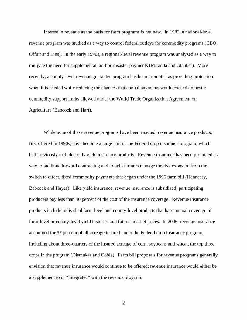
Interest in revenue as the basis for farm programs is not new. In 1983, a national-level

revenue program was studied as a way to control federal outlays for commodity programs (CBO;

Offutt and Lins). In the early 1990s, a regional-level revenue program was analyzed as a way to

mitigate the need for supplemental, ad-hoc disaster payments (Miranda and Glauber). More

recently, a county-level revenue guarantee program has been promoted as providing protection

when it is needed while reducing the chances that annual payments would exceed domestic

commodity support limits allowed under the World Trade Organization Agreement on

Agriculture (Babcock and Hart).

While none of these revenue programs have been enacted, revenue insurance products,

first offered in 1990s, have become a large part of the Federal crop insurance program, which

had previously included only yield insurance products. Revenue insurance has been promoted as

way to facilitate forward contracting and to help farmers manage the risk exposure from the

switch to direct, fixed commodity payments that began under the 1996 farm bill (Hennessy,

Babcock and Hayes). Like yield insurance, revenue insurance is subsidized; participating

producers pay less than 40 percent of the cost of the insurance coverage. Revenue insurance

products include individual farm-level and county-level products that base annual coverage of

farm-level or county-level yield histories and futures market prices. In 2006, revenue insurance

accounted for 57 percent of all acreage insured under the Federal crop insurance program,

including about three-quarters of the insured acreage of corn, soybeans and wheat, the top three

crops in the program (Dismukes and Coble). Farm bill proposals for revenue programs generally

envision that revenue insurance would continue to be offered; revenue insurance would either be

a supplement to or “integrated” with the revenue program.

2

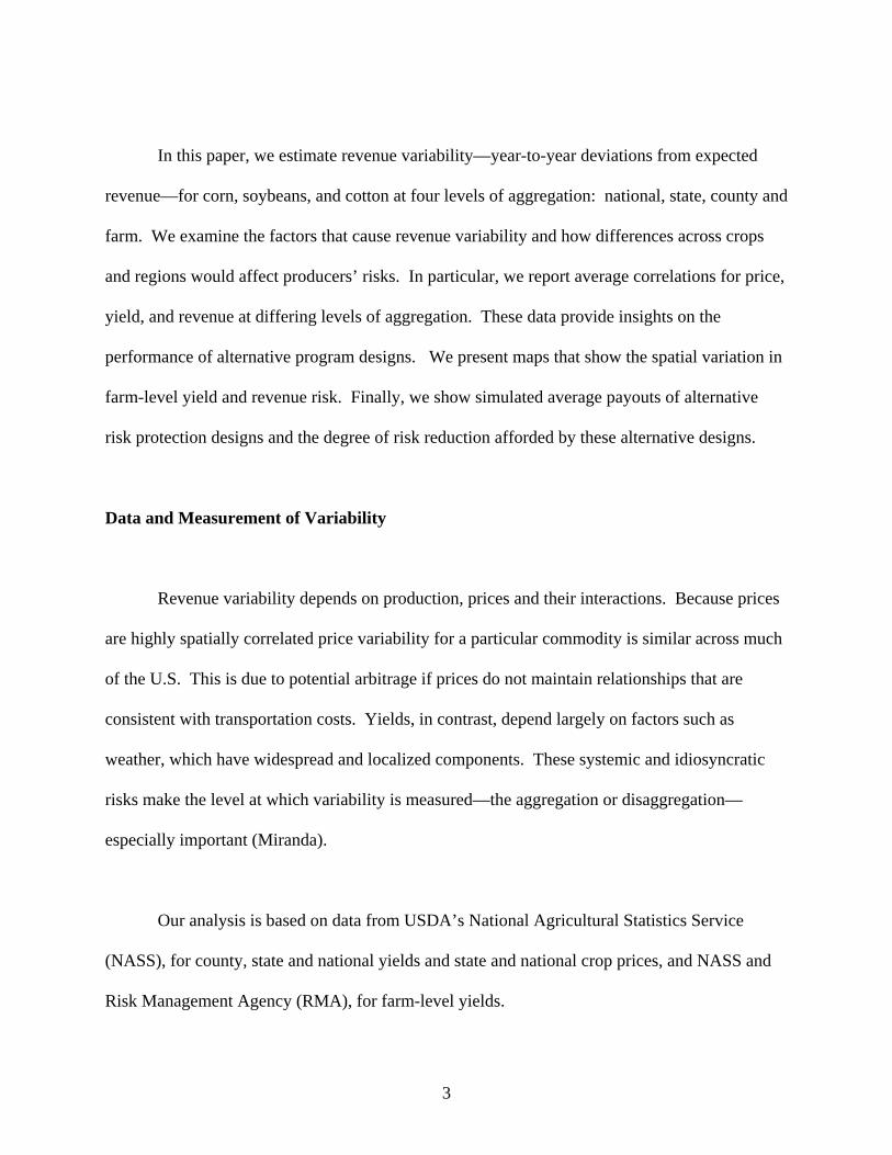
In this paper, we estimate revenue variability—year-to-year deviations from expected

revenue—for corn, soybeans, and cotton at four levels of aggregation: national, state, county and

farm. We examine the factors that cause revenue variability and how differences across crops

and regions would affect producers’ risks. In particular, we report average correlations for price,

yield, and revenue at differing levels of aggregation. These data provide insights on the

performance of alternative program designs. We present maps that show the spatial variation in

farm-level yield and revenue risk. Finally, we show simulated average payouts of alternative

risk protection designs and the degree of risk reduction afforded by these alternative designs.

Data and Measurement of Variability

Revenue variability depends on production, prices and their interactions. Because prices

are highly spatially correlated price variability for a particular commodity is similar across much

of the U.S. This is due to potential arbitrage if prices do not maintain relationships that are

consistent with transportation costs. Yields, in contrast, depend largely on factors such as

weather, which have widespread and localized components. These systemic and idiosyncratic

risks make the level at which variability is measured—the aggregation or disaggregation—

especially important (Miranda).

Our analysis is based on data from USDA’s National Agricultural Statistics Service

(NASS), for county, state and national yields and state and national crop prices, and NASS and

Risk Management Agency (RMA), for farm-level yields.

3

To measure variability of yields at the county, state and national levels, we estimated a

linear time trend from each NASS 1975-2004 yield data series and calculated variability from the

residuals relative the predicted yield for 2006. Given detrended national, state, and county yield

series, we next computed farm yield variability for a representative for each county. This

representative farm is assumed to have a mean yield equal to the expected county yield and yield

variability consistent with the average riskiness of farms insured by RMA’s crop insurance yield

insurance. Given the average premium rate for 65 percent coverage yield insurance for each

crop in each county, we search for a multiplier, k, which will expand county yield variability to a

level that generates the RMA premium rate.

df = dc * k (1)

where df is farm yield deviation from expectation and dc is the deviation in county yield from

expectation and k is an expansion factor. The expansion factor accounts for the disaggregation

effect, the increase in variability between the county and average farm yield. Therefore, using

the crop insurance premium rate, a grid search from 1.0 to 5.0 by intervals of 0.2 was conducted

to find the yield variability that most closely approximates the crop insurance premium rate1.

For example, Bolivar County in Mississippi has an expansion factor of 2.8 for cotton while

cotton in Coahoma County, Mississippi, has an expansion factor of 2.4. Once this equation is

established, the matrix [Yf] is created, which has county and farm yields with T1 rows for each

year and N county columns.

1 Crop insurance is generally sold at the basic or optional unit level, which is typically more disaggregated than the farm. Thus, the effective premium rate data is largely a mix of basic and optional unit rates. The effective premium rates were adjusted downward by 15 percent to approximate farm-level variability.

4

Price variability is estimated from NASS data. National annual marketing-year

average (MYA) prices for 1974 through 2005 are used. State basis adjustments from the national

price are also derived from the historical data. The simulation uses 500 random draws of a five-

year time path. Yields and prices for every location are drawn simultaneously to maintain the

empirical correlations between prices and yields and between yields at different levels of

aggregation. Starting prices for the simulations are determined from December 2006 futures

market prices for 2007 delivery months. The MYA price is obtained by taking the relative price

change associated with the randomly drawn yield shock and multiplying by the previous year’s

MYA price. State prices are obtained by adjusting national price for a regional basis. Five

hundred iterations are used, resulting in 2,500 random draws for each location (five years

multiplied by 500 iterations).

Farm program payments are calculated based on the simulated prices and yields.

Program parameters such as direct payment rates, loan rates, coverage percentages, and target

prices are specified as described in the various programs. Planted acreage is obtained from

NASS for the 2005 crop year. Base acreage for 2002 for each county is obtained from the Farm

Service Agency. Base yields are derived by comparing the national average base yield to the

expected yield. This ratio is applied to the 2007 expected yield for each county.

The current farm programs included in our analysis are Direct Payments (DPs), Loan

Deficiency Payments (LDPs), and Counter-Cyclical Payments (CCPs). To calculate the DP:

BADPDPyDP PRf ***ˆ= (2)

5

where is the predicted farm yield for 2006, DPfy R is defined as the direct payment rate, DPP is

the direct payment percentage and BA is base acreage. The additional information needed to

calculate LDPs is the loan rate parameter. To calculate LDPs:

PAMYALRyLDPs f *),0max(* −= (3)

LR stands for the loan rate and PA represents planted acres. The CCP is calculated as:

( ) BAMYALRDPCCPDPyCCPCCP RTPRfP *),max(**ˆ* −−= (4)

CCP percentage is CCPP; CCPTP is the CCP target price.

We also model programs that would be based on expected revenue for the each of the

three crops: corn, soybeans and cotton. We model two designs that would trigger payments

based on aggregate revenue shortfalls: one that would use national-level aggregate revenue and

another that would use county-level revenue. Each of these designs would guarantee 95 percent

of expected revenue:

))(**95.0,0max(RevGuar iiiii YPYEEP −= (5)

where EP is the expected price, E(Y) is the expected yield. When i = N a national program

trigger is used and when i = C a county trigger is used.

As a third option we model an area-revenue program integrated with farm-level revenue

insurance. Integration of the program with insurance means that revenue program payments

would be deducted from any insurance indemnity payments. The area revenue program would

cover the systemic portion of the loss and the farm insurance would cover the idiosyncratic. This

is sometimes referred to “wrap around” coverage. The program design that we model combines

the national-level 95-percent revenue guarantee with a 75-percent farm-level guarantee, a farm-

6

level coverage insurance currently available under the Federal crop insurance program. The

integrated or wrap around payment is calculated:

))RevGuar()(*),max(*75.0,0max(Wrap iiii YPYEHPEP +−= (6)

Results

For the three crops in the study, national-level revenue variability is nearly double

national-level yield variability (Table 1). This is because yield variability is greatly dampened

by spatial aggregation, while price variability is not; price variability pulls national revenue

variability upward. Spatial disaggregation increases price and yield variability, but yield

variability increases more rapidly than price and revenue variability. The result is that at the

farm-level, revenue variability is typically only about 10 percent higher than yield variability.

Across the crops, cotton yield and revenue variability are highest among the crops at all levels of

aggregation.

To further understand the factors underlying the results in table 1, we report, in tables 2A

through 2C, the average correlation coefficients between yield, price, and revenue for each of the

three crops. The correlations reported in these tables are acre-weighted average correlations.

For example, the reported correlation between farm and national yield is the acre-weighted

average of correlations between farm and national yield for the entire United States given that

there are several hundred farm-level observations.

7

In table 2A we report the results for corn. The upper portion of the table reports the

average correlations for yields at various levels of aggregation. The national corn yield on

average is positively correlated on average with corn yields at the state, county and farm levels,

but the correlation becomes weaker as one compares the national yield with yields at smaller

units of aggregation. The average correlation between national yield and state yield is 0.414 and

drops to 0.315 for the average county and 0.286 for the average farm. Average correlation

between national average corn price and national yield is -0.381 and weakens at smaller units. It

drops by more than half to -0.117 when one goes to the state level yield and drops further, to -

.064, at the farm level. In the lower portion of the table we report correlation of revenue at

various levels of aggregations, and between revenue, price, and yield. These are particularly

important when one considers the risk reduction afforded by various revenue triggered programs.

We pay particular attention to the correlation between farm level revenue and the revenue at

other levels. For corn the average correlation between farm revenue and county revenue is

0.888. And on average the correlation between farm revenue and state revenue is 0.739. It

remains relatively high, 0.56, as one examines the correlation between farm revenue and national

revenue.

The correlations for soybeans (Table 2B) are similar to those for corn. Yields are

positively correlated with each other and prices are negatively correlated with yield at all levels

of aggregation. The farm yield average for soybeans correlated with national yield at a 0.264

level, a slightly weaker correlation than for corn. At the county and state levels correlations with

national yields for soybeans are slightly stronger than for corn, however. The national level

price-yield correlation for soybeans is -0.386, similar to the same correlation for corn. The

8

average correlation between national price and yield drops by more than half, to -0.179, as one

moves to the state level and to -0.096 at the farm level. Correlation of soybean revenue with

national price is strong, 0.959 and about equal to the similar correlation for corn. As one moves

to more disaggregate units the correlation between national soybean revenue and the unit’s

revenue declines, to 0.828 at the state level, 0.764 at the county level and 0.503 at the farm level.

Correlations between national cotton yield and yields at disaggregated levels (Table 2C)

in general tend to be weaker than those for corn and soybeans. The average correlation of state

cotton yield to national cotton yield is 0.275 and it declines to 0.239 when national yield is

correlated with average county yield. And the correlation between the average farm and national

yield is 0.188. While cotton shows negative relationships between yield and price, the

magnitude tends to be relatively small. Even at the national level, the correlation between

national yield and national price is -0.144. This declines rapidly as one goes to the state level

and drops off to an average correlation of -0.027 between farm yield and national price. Cotton

revenue correlations show patterns similar to those of corn and soybeans. However, the

relationship between national revenue and national price, 0.798, is somewhat lower than for corn

and soybeans. Likewise, the correlation between state, county, and national revenue is less than

it is for corn and soybeans. For example, the average correlation between national revenue and

state revenue is 0.387, which declines to 0.263 at the farm level.

To examine the spatial distributions of farm-level yield and revenue variability we

present maps (Figures 1 – 6) of the average, at the county level, coefficient of variation of each

of these farm-level variables for corn, soybeans and cotton. In these maps counties shaded green

9

have relatively low variability at the farm-level (coefficient of variation less than 30 percent).

Those shaded red have the greatest variability (coefficient of variation greater than 50 percent)

and those shaded yellow and orange have intermediate variability (30 – 40 percent and 40 – 50

percent).

Not surprisingly the Corn Belt is largely defined by the low level of yield risk observed in

that region. Counties with the lowest farm-level yield coefficient of variation are spread from

southern Minnesota through Iowa, Illinois, Indiana, and Ohio (Figure 1). In the regions at the

fringes of the Corn Belt, and also in the southern and eastern state, the coefficient of variation

typically nears or exceeds 50 percent. The pattern of revenue variability is similar to that of

yield variability, though fewer counties that have a revenue coefficient of variation less than 30

percent (Figure 2). Still, the counties with high revenue variability tend to be those with high

farm-level yield variability.

The soybean yield variability pattern (Figure 3) is similar to pattern for corn. The heart

of the Midwest has the lowest coefficient of variation. When one turns to farm-level revenue

coefficient of variations for soybeans (Figure 4) the pattern of revenue coefficient of variation, as

with the other two crops, is very similar to yield.

Farm-level yield variability for cotton (Figure 5) differs dramatically across the U.S.

Most of Texas has high coefficients of variations, while the lowest farm-level yield coefficients

of variations are in California. The pattern of revenue coefficient of variation for cotton (Figure

6) is similar to the farm-level yield coefficient of variation pattern. The counties with the lowest

10

farm-level revenue coefficient of variation are in California, while Texas and portions of the

southeast United States have the highest farm-level revenue coefficient of variation.

Having investigated the underlying variability and correlations of various relevant

random prices, yields and revenue, we next report farm program benefits that would be

determined by these random variables. Table 3A reports simulations of the farm program

payments that would occur over the 2008-2012 period if current programs remain in place. The

results reported are five-year average payments per planted acre.

Our analysis, suggests that a continuation of the current DP program, which does not

respond to either price or yield shortfalls, would average about $22.51 per acre for corn, $11.21

per acre for soybeans and $32.30 per acre for cotton. The other commodity programs—CCP,

LDP and Federal crop insurance—are characterized as risk mitigating programs because

payments are related to declines in prices or yields. Of these programs, the CCP program for

corn and soybeans both pay in the neighborhood of $2 per acre per year. These low payments

are partly due to predicted high prices for corn and soybeans over the next several years. In

contrast, prices for cotton are lower relative to the current target price and the CCPs for cotton

would be expected to average $32.30 per year. The LDP program is expected to pay $1.15 per

acre for corn, $5.29 for soybeans and $8.17 for cotton. The crop insurance program indemnity

payments, net of producer paid premium, assume that the producer participates at the 65 percent

yield coverage level. For corn, the average net indemnity would be slightly over $12 per acre;

for soybeans, it would be near $7.25 per acre; for cotton, it would be slightly less than $17 per

11

acre. In total across these current programs would be expected to pay $37.65 per acre for corn,

$26 per acre for soybeans, and slightly over $90 per acre for cotton.

Table 3a reports the expected payments for revenue programs guaranteeing 95 percent of

expected revenue calculated with a national and with a county level trigger. We also examine

the case of where the national level revenue program is integrated with a 75-percent individual

insurance coverage. In the case of corn, the national revenue trigger program would pay

approximately $3.61 per acre, whereas a county triggered program would average paying slightly

under $25 per acre because of the greater revenue variability of county revenue. In a similar

fashion for soybeans, we find that the national revenue program would pay approximately $3.80

per acre, while we estimate the county revenue program would pay $22.43 per acre on average.

Cotton has an expected payout based on 95 percent of expected national revenue of $8.81 per

acre, and a county triggered program for cotton would approximately triple the payout to $25.88

per acre. If we add a farm level 75 percent guarantee integrated with the national revenue

program, we see a payment of slightly over $6 per acre for corn, slightly more than $3 per acre

for soybeans, and $21.42 per acre for cotton.

How well would these programs reduce revenue variability at the farm level? In table 3b

we report risk reduction, calculated as the percentage decrease in the farm-level revenue

coefficient of variation. Given current farm programs, and the hypothetical national, county and

farm revenue programs, our analysis suggests that the reduction in the revenue coefficient of

variation for the current programs range from slightly more than 14 percent for corn up to

slightly more than 33 percent for cotton. Under a national revenue trigger program, the average

12

risk reduction for farms in our analysis would be slightly more than 8 percent for corn, about 7

percent for soybeans and about 21 percent for cotton. In all three cases, the coefficient of

variation is reduced less with the national revenue triggered program than by current programs.

However, if one integrates the nationally triggered revenue program with 75 percent farm-level

revenue coverage the percent risk reduction more than doubles for both corn and soybeans.

Although the increase in risk reduction between the national and the integrated program is

proportionately less for cotton, the total risk reduction for cotton, nearly 35 percent, is the

greatest among the three crops.

The spatial distribution of the risk reduction from alternative revenue program designs is

illustrated in figures 7, 8 and 9. We show the risk reduction at the farm level as one moves from

a 95 percent national revenue program to 95 percent county revenue program for corn (Figure 7),

for soybeans (Figure 8) and for cotton (Figure 9). In these maps an area that is shaded red has a

county triggered risk reduction that is within five percent of the risk reduction afforded by a

nationally triggered program. The orange shaded counties fall between 105 and 110 percent of

the U.S. program’s risk reduction. Counties shaded yellow have risk reduction that is between

10 and 20 percent higher than the U.S. program. And those counties that are shaded green have

a risk reduction from a county triggered program that exceeds 120 percent of the risk reduction

of the nationally triggered program. These analyses give an indication of how correlation

between the triggering programs influences the risk reduction that producers are able to obtain.

In figure 7, it is shown that in the heart of the Corn Belt, a commodity program triggered by

national revenue shortfalls would provide a degree of risk reduction that is similar to a county

triggered program. However, as one moves into regions away from the heart of the Corn Belt,

13

the county triggered program tends to produce at least 20 percent more risk reduction than the

nationally triggered program.

Figure 8 reports the relative risk reduction of a county-triggered program versus a

nationally triggered program for soybeans. Similar to the map for corn, a national program for

soybeans performs more effectively relative to a county program in the heart of the Corn Belt.

Counties where a county triggered program provides much better risk protection are in regions

such as Eastern Kansas and much of the Southeast where the correlation with national revenue is

weaker.

Figure 9 reports the risk reduction obtained by a county versus a national revenue

triggered program for cotton. In this case the nationally triggered program tends to do

reasonably well for the Mid-south, with a risk reduction that is generally within 10 percent of

that obtained by the county program. However, in much of Texas and in the southeast region,

the county triggered program would do a much better job than the nationally triggered program.

Implications

The discussion of revenue-based commodity programs as a farm policy tool has reached

a new level during the 2007 farm bill debate. This discussion should recognize that the

fundamental statistical patterns of revenue risk profoundly influence the effects of the various

proposals. Revenue risk differs from price risk in the magnitude of variability; the underlying

yield variability varies significantly across crops and is affected differently by aggregation. For

14

example, revenue variability is greater at the national level than price variability suggesting that,

all else equal, national revenue trigger programs would generally pay more than price triggered

programs. Likewise, all else equal, moving from a nationally-triggered program to a state or

county-triggered program will be more costly for government because on average disaggregation

increases revenue risk.

A related issue is the degree of correlation between the revenue triggered program

payments and actual losses at the producer level. While producer interest in revenue based

designs seems to be strongest where producers see a negative price-yield correlation in their

locality, the heart of the Corn Belt, for example, revenue payments would tend to be largest for

crops in regions where yield risk is largest and the price-yield correlation does not dampen

revenue variability, that is, areas away from the major production regions.

Our results show several important points for the design of revenue programs. First,

when the revenue trigger is weakly correlated with farm revenue it provides less effective risk

reduction, a situation that is analogous to basis risk in a futures market. Second, the strength of

the price-yield correlation suggests the degree to which a revenue program would make

payments when a producer has a revenue loss and, conversely, the degree to which a revenue

program would not make a payment when a producer does not have a loss. This feature could

make a revenue program more effective at reducing risk than separately triggered price and yield

programs. Replacement of price and yield programs with a revenue program, however, would

have major implications for the largely separate program delivery systems—the Farm Service

15

Agency for the commodity price-based programs and the private crop insurance companies that

sell and adjust Federal crop insurance policies.

16

REFERENCES

American Farm Bureau Federation. “Farm Bill: An Investment That’s Working. Farm Bureau’s Recommendations for the 2007 Farm Bill.” 56 pages. released April 23, 2007. http://www.fb.org/newsroom/farmbill2007/AFBF2007FBProposal.pdfaccessed April 25, 2007 American Farmland Trust. “Agenda 2007: A New Framework and Direction for U.S. Farm Policy.” American Farmland Trust, Washington, DC. 2006. http://www.farmland.org/documents/AFT_Agenda2007_May06.pdfaccessed April 13, 2007 Bruce A. Babcock and Chad E. Hart. “How Much Safety is Available under the U.S. Proposal to the WTO?” Center for Agricultural and Rural Development Briefing Paper 05-BP 48, November 2005. http://www.card.iastate.edu/publications/DBS/PDFFiles/05bp48.pdf Congressional Budget Office. Farm Revenue Insurance: An Alternative Risk-Management Option for Crop Farmers. August 1983. 32 pages. Robert Dismukes and Keith H. Coble. “Managing Risk with Revenue Insurance.” Amber Waves. USDA. November 2006. David A. Hennessy, Babcock, B.A. and Hayes, D. J. “Budgetary and Producer Welfare Effects of Revenue Insurance.” American Journal of Agricultural Economics, Vol. 79, No. 3 (Aug., 1997), pp. 1024-1034. Mario J. Miranda. Area-Yield Crop Insurance Reconsidered. American Journal of Agricultural Economics, Vol. 73, No. 2 (May, 1991), pp. 233-242 Mario J. Miranda and Joseph W. Glauber. Providing Crop Disaster Assistance through a Modified Deficiency Payment Program. American Journal of Agricultural Economics, Vol. 73, No. 4 (Nov., 1991), pp. 1233-1243 National Association of Corn Growers. “Forging a New Direction for Farm Policy.” http://ncga.com/news/notd/pdfs/10_23_06NFSA.pdfaccessed April 13, 2007. Susan E. Offutt and David A. Lins. “Income Insurance for U.S. Commodity Producers: Program Issues and Design Alternatives.” North Central Journal of Agricultural Economics. Vol. 7, No. 1. January 1985. U.S. Department of Agriculture. Farm Bill Proposal. USDA 2007 Farm Bill Proposals. 183 pages. January 31, 2007. http://www.usda.gov/documents/07finalfbp.pdfaccessed April 13, 2007

17

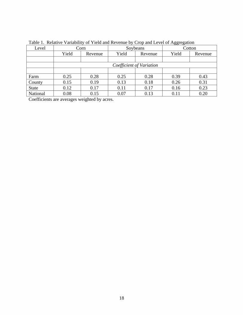
Table 1. Relative Variability of Yield and Revenue by Crop and Level of Aggregation

Level Corn Soybeans Cotton Yield Revenue Yield Revenue Yield Revenue Coefficient of Variation Farm 0.25 0.28 0.25 0.28 0.39 0.43 County 0.15 0.19 0.13 0.18 0.26 0.31 State 0.12 0.17 0.11 0.17 0.16 0.23 National 0.08 0.15 0.07 0.13 0.11 0.20 Coefficients are averages weighted by acres.

18

Table 2a. Corn: Correlation Coefficients of Yield, Price and Revenue by Level of Aggregation Yield Price Revenue Farm County State National Farm County State National Yield: Farm 1.000 County 0.890 1.000 State 0.671 0.713 1.000 National 0.286 0.315 0.414 1.000 Price -0.134 -0.088 -0.117 -0.281 1.000 Revenue: Farm 0.799 0.721 0.527 0.255 0.453 1.000 County 0.544 0.652 0.431 0.033 0.677 0.888 1.000 State 0.316 0.374 0.530 0.038 0.767 0.739 0.859 1.000 National 0.010 0.012 0.015 0.038 0.946 0.560 0.718 0.813 1.000 Price is marketing year average price at national level. Table 2b. Soybeans: Correlation Coefficients of Yield, Price and Revenue by Level of Aggregation Yield Price Revenue Farm County State National Farm County State National Yield: Farm 1.000 County 0.870 1.000 State 0.714 0.812 1.000 National 0.264 0.353 0.429 1.000 Price -0.096 -0.147 -0.179 -0.363 1.000 Revenue: Farm 0.775 0.690 0.531 0.197 0.411 1.000 County 0.409 0.540 0.388 -0.074 0.733 0.840 1.000 State 0.245 0.352 0.434 -0.077 0.794 0.718 0.916 1.000 National -0.078 -0.053 -0.066 -0.095 0.959 0.503 0.764 0.828 1.000 Price is marketing year average price at national level.

19

Table 2c. Cotton: Correlation Coefficients of Yield, Price and Revenue by Level of Aggregation Yield Price Revenue Farm County State National Farm County State National Yield: Farm 1.000 County 0.894 1.000 State 0.742 0.860 1.000 National 0.175 0.188 0.239 1.000 Price -0.045 -0.027 -0.029 -0.144 1.000 Revenue: Farm 0.969 0.870 0.722 0.306 0.158 1.000 County 0.844 0.950 0.816 0.138 0.254 0.894 1.000 State 0.681 0.797 0.928 0.173 0.320 0.746 0.870 1.000 National 0.068 0.089 0.119 0.474 0.798 0.263 0.307 0.387 1.000Price is marketing year average price at national level.

20

Table 3a. Average Simulated Payments, Current Programs and National, County and Farm Revenue Programs Corn Soybeans Cotton Dollars per Acre Current Programs: Direct Payment 22.51 11.21 32.30 Counter-Cyclical Payment 1.94 2.26 32.30 Loan Deficiency Payment 1.15 5.29 8.17 Crop Revenue Insurance Indemnity 12.04 7.25 16.92 ---Total 37.65 26.00 90.04 Revenue Programs: National 3.61 3.80 8.81 County 24.96 22.43 25.88 National with Farm 6.08 3.12 21.42National and county revenue programs are based on 95 percent of expected revenue. Farm revenue program is based on 75 percent of expected revenue. Table 3b. Simulated Reduction of Risk at Farm Level from Current Programs and National, County and Farm Revenue Programs Corn Soybeans Cotton Percent Decrease in Coefficient of Variation Current Programs 14.34 17.09 33.24 Revenue Programs: National 8.14 6.97 20.95 County 14.65 8.58 24.76 National with Farm 19.85 19.30 34.73 National and county revenue programs are based on 95 percent of expected revenue. Farm revenue program is based on 75 percent of expected revenue.

21

Figure 1. Corn Farm-Level Yield Coefficient of Variation

Figure 2. Corn Farm-Level Revenue Coefficient of Variation

22

Figure 3. Soybean Farm-Level Yield Coefficient of Variation

Figure 4. Soybean Farm-Level Revenue Coefficient of Variation

23

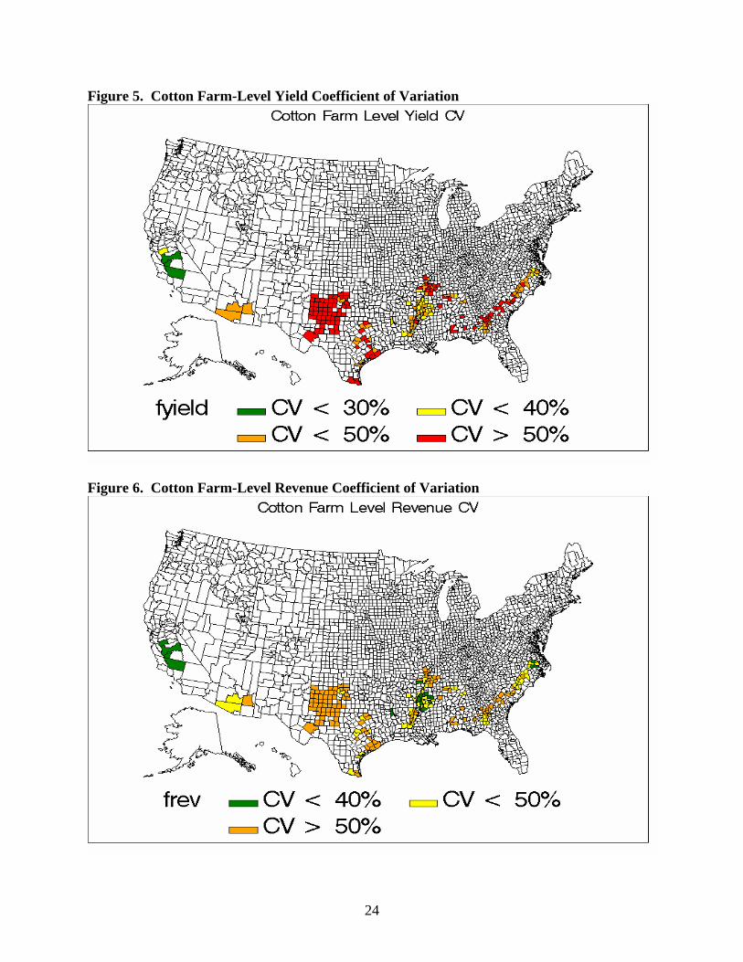
Figure 5. Cotton Farm-Level Yield Coefficient of Variation

Figure 6. Cotton Farm-Level Revenue Coefficient of Variation

24

Figure 7

25

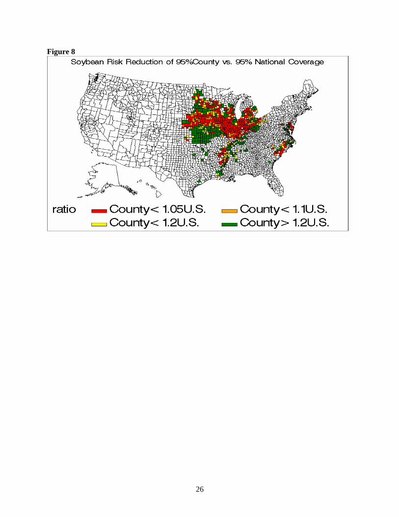
Figure 8

26

Figure 9

27