Air Cargo Revenue Management

Air Cargo Revenue Management

introducing

Unified Density 0|1Scaled Density o|∞


Proefschrift

ter verkrijging van de graad van doctor aan de Universiteit van Tilburg,

op gezag van de rector magnificus,

Prof. dr. F.A. van der Duyn Schouten, in het openbaar te verdedigen ten overstaan van een door

het college voor promoties aangewezen commissie in de aula van de Universiteit

op vrijdag 24 november 2006 om 10:15 uur door

Johannes Blomeyer

geboren op 3 mei 1961 te Frankfurt/Main, Duitsland.

Promotores:

Professor Dr. ir. Hein FleurenProfessor Dr. Jan Bisschop

Printed in Germany. First edition. Proofreading: Giles Stacey (Englishworks)© 2006 Johannes Blomeyer. All rights reserved.

No part of this book may be reproduced without the written permission of the author. Unauthorised duplication is a violation of applicable laws.

While every precaution has been taken in the preparation of this book, the author assumes no responsibility for errors or omissions, or for damages resulting from the use of the information contained herein. In no event shall the author be liable for any loss of profit or any other commercial damage, including but not limited to special, incidental, consequential, or other damages.


Johannes Blomeyer

Dedication

To the country and the people I love most—Colombia.

Acknowledgements

I would like to thank Professor Dr. Hein Fleuren, who supported me from day one and has not stopped since. Many thanks, too, to Professor Dr. Jan Bisschop without whom there would not have even been a day one—and to Ms. Selvy Suwanto from Paragon Decision Technology B.V. for program-ming several versions of the Segment Optimiser in the mathematical pro-gramming language AIMMS. On a more personal level, I would also like to thank my colleagues at Lufthansa.

Preface

Goethe in his ‘Farbenlehre’ associated blue with infinity and saw it as the color of transcendence. Jung associated blue with the vertical, the blue sky above and the blue ocean below; he saw a correspondence with the un-conscious. Yves Klein postulated Monochrome IKB (International Klein Blue) as the color of the universe and hoped to use it to sensitize the whole planet. At about the same time Yuri Gagarin, the first cosmonaut, looked at us from outer space and reported: “The earth is blue.”

This text by Siegfried Loch, printed on the cover of Jasper van’t Hof ’s musical recording “Blue Corner” (ACT 1996, Hamburg), encouraged me to write about Cargo Revenue Management from many different viewpoints—just as Siegfried Loch wrote about blue.

April, 2006Johannes Blomeyer

Table of Contents

.....................................................................Air Cargo Revenue Management+ 1

Part I: Introduction

..............................................................1 Revenue Management in Air Cargo+ 3..................................................................................................1.1 Introduction+ 3

......................................................................................................1.2 Literature+ 8

.........................................................................................2 Preliminary Notes+ 15......................................................................................................2.1 Notation+ 15

....................................................................2.2 Primary and Secondary Units+ 15

Part II: Air Cargo Properties

...............................................3 Initial and Derived Properties in Air Cargo+ 19...................................................................3.1 Weight, Volume, and Revenue+ 19

................................3.2 Density, Standard Density, and Chargeable Weight+ 193.3 Weight Coefficients, Volume Coefficients,

...................................................... and the Rate per Chargeable Weight+ 30.........................3.4 Numerical Examples of Initial and Derived Properties+ 32

...........................................3.5 Simple Set of Derived Air Cargo Properties+ 34......................................3.6 Extended Set of Derived Air Cargo Properties+ 36

..............................................................................................3.7 Contribution+ 39

Part III: Overview of Revenue Management in Air Cargo

......................................4 Basics of a Cargo Revenue Management System+ 41...........................................................................4.1 Flight, Segment, and Leg+ 41

...........................4.2 Flight Revenue, Segment Demand, and Leg Capacity+ 43.................................4.3 Booking Process, Booking, and Booking Request+ 46

.........................................4.4 Instruments in Cargo Revenue Management+ 51..............................................................................................4.5 Contribution+ 56

Part IV: Nonlinear Density Scaling

....................................................................5 Various Densities in Air Cargo+ 59............................................................................................5.1 Linear Density+ 59

........................................................5.2 Unified Density and Scaled Density+ 61..............................................................................................5.3 Contribution + 70

Part V: Forecasting, Optimisation, and Control

.......................................................................6 Segment Demand (Forecast)+ 73.........................................6.1 Segment Demand and Demand Distribution+ 73

.............................................................................6.2 Rate-Density Domains+ 78.................................................................................6.3 Demand Aggregation+ 83

...................................................................................6.4 Rate-Density Grids+ 89..............................................................................................6.5 Contribution+ 91

......................................................................7 Flight Revenue Optimisation+ 93................................7.1 Primal Model to Calculate the Revenue of a Flight+ 94

..................................7.2 Dual Model to Calculate the Revenue of a Flight+ 99................7.3 Kuhn-Tucker Conditions and the Optimal Flight Revenue+ 104

.........................7.4 Rate-Density Grids and the Optimal Flight Revenue+ 107............................................................................................7.5 Contribution + 109

...........................................................................8 Booking Request Control+ 111......................................................................8.1 Marginal Bid Price Control+ 111

........................................................................8.2 Lumpy Bid Price Control+ 114.......................................................8.3 Booking Request Control Overview+ 115

............................................................................................8.4 Contribution+ 124

..........................................9 Booking Request Control with Stowage Loss+ 125...............................................................................9.1 Volume Stowage Loss+ 125

...........................................9.2 Stowage Loss and Optimal Flight Revenue+ 131.........................................................9.3 Maximal Acceptable Stowage Loss + 133

............................................9.4 Stowage Loss and the Primal-Dual Graph+ 136.............................................................................................9.5 Contribution+ 141

............................................................................Summary and Conclusions+ 142

Appendix

..............................................................................................List of Symbols+ 144.................................List of Mathematical Programs, Figures, and Tables+ 148

...................................................................................................Bibliography+ 150..............................................................................................................Index+ 160

..........................................................................................................Abstract+ 166..................................................................................................Samenvatting+ 167

..........................................................................................About the Author+ 169


This dissertation is about Air Cargo Revenue Management: the Revenue Management of the air cargo industry. One of the most basic definitions of Revenue Management is from Kimes (2001, page 3): “Yield Management [or Revenue Management, for that matter] is a method which can help a firm to sell the right inventory unit to the right type of customer, at the right time and for the right price. Yield Management guides the decision of how to allocate undifferentiated units of capacity to available demand in such a way as to maximize profit or revenue. The problem then becomes one of determining how much to sell at what price and to which market segment.” Another definition, and one which is more suited to the airline industry, is by Garvett and Hilton (1999, page 181): “Good revenue maxi-mizers seek to obtain the best possible yields and load factors given the cir-cumstances. Yet it is easy to get high yields by excessively raising fares and limiting the availability of discounts—and in the process ensuring nearly empty flights. Similarly, it is easy to maximize load factors by giving the product away. Neither strategy will lead to profitability […]. The art is to obtain both high load factors and high yields at the same time” (as quoted in O’Connor 2001, page 133)—or, more precisely, to obtain the highest pos-sible revenue.

This dissertation has nine chapters which are clustered into five parts. Part I is the introduction, Part II is about air cargo properties, Part III is an overview of Revenue Management in air cargo, Part IV concerns nonlinear density scaling, and Part V is about forecasting, optimisation, and control.

More specifically, the dissertation is organised as follows: the first chapter introduces Air Cargo Revenue Management in general and gives an over-view of the existing literature on the subject. The second chapter contains some preliminary notes about notation and quantity units, while the third chapter presents the initial and derived properties of items related to air cargo. The elements and instruments of a Cargo Revenue Management System are introduced in the fourth chapter, and the fifth chapter presents the concept of unified density. Segment demand and flight revenue are dis-cussed in the sixth and the seventh chapters. The subject of Chapter 8 is the control of booking requests in air cargo, and booking request control linked to stowage loss is the focus of the ninth chapter. The dissertation ends with a summary and conclusions.

1

PART I: INTRODUCTION

1 Revenue Management in Air Cargo

The idea of managing revenues in the airline industry originated in the pas-senger sector and was first applied in the 1980s. Since then, there have been many attempts to transfer these techniques to other industries, in-cluding but not limited to air cargo, rail cargo, ocean cargo, and tour opera-tors.

Even though the management of cargo revenue is considered to be a disci-pline in its own right, it belongs to the class of Network Revenue Manage-ment problems because Cargo Revenue Management Systems typically in-volve the quantity-based management of multiple resources. In further specifying the subject, Talluri and van Ryzin writing about Network Reve-nue Management stated: “When products are sold as bundles [as is the case in air cargo, because a cargo booking consumes weight and volume], the lack of availability of any one resource in the bundle limits sales. This cre-ates interdependence among the resources, and hence, to maximize total revenues, it becomes necessary to jointly manage (co-ordinate) the capacity controls on all resources” (Talluri and van Ryzin 2004, page 81). It should be noted that a Revenue Management problem does not need to have an explicit network structure to be considered as a Network Revenue Man-agement problem (ibid., page 81).

Furthermore, there is an important difference between Revenue Manage-ment and Pricing: applying quantity-based Revenue Management tech-niques and the act of setting prices are two different things because a quan-tity-based Cargo Revenue Management System does not perform freight pricing. Quantity-based Cargo Revenue Management Systems assume that the products have fixed prices and that booking control manages only the allocation of the resources to the different products (as is, incidentally, the assumption with all quantity-based Revenue Management Systems; Talluri and van Ryzin 2004, page 81).

Starting with an introduction, this chapter is divided into two sections. The first section introduces Cargo Revenue Management in general, and the second gives an overview of the existing literature insofar as it is relevant to the subject matter.

1.1 Introduction

Since many of the concepts in Cargo Revenue Management originated from Passenger Revenue Management, it is helpful to look at the differ-ences and commonalities between passengers and cargo. Before this, how-ever, the demand for air cargo and the specifics of transporting air cargo are discussed.

3

The Demand for Air Cargo

To start with a definition, O’Connor defines air cargo as follows: “The term air cargo is generally used in the broad sense, to include airfreight […], mail, and the several types of expedited small package services to which the term air express is now rather loosely applied” (O’Connor 2001, page 153). Passen-ger baggage on passenger flights is, however, not considered as air cargo.

The demand for air cargo has grown steadily over the past 20 years, and this growth is expected to continue into the future. The goods which are transported by air are as diverse as car parts, live animals, and human re-mains, and most of the cargo traffic is between Europe, Asia, and the United States of America.

Air cargo is, of course, not the only means of transporting freight from A to B, so there is competition. O’Connor (2001, page 180) wrote about the competitors: “Competition with other modes means, as a practical matter, with ocean vessels and with trucks. While railroads carry more in sheer ton-miles of cargo than trucks, nowadays it is of a sort that is not divertible to air: low-value-per-ton commodities such as coal, ores, and grain. The truck, being substantially more expensive than the train yet offering what is usually a much faster service, is the carrier of the high-value-per-ton traf-fic, mostly merchandise and other manufactured or partly processed goods, from which air diverts.” Further, about the competition between vessels and airplanes, he wrote (ibid., page 182): “Various estimates indicate that transportation of the high-value goods for which air and ocean compete, carried on fast modern container vessels, may cost the shipper anywhere between one-tenth and one-third of what it would cost if shipped by air (see Air Cargo World 1996, page 20).” However, “the gap between the two modes with respect to time is far greater. Ship transport may take 10 or 20 days to move cargo where air would take only a day or two. The time ad-vantage by air is so great—so much greater than air’s time advantage over truck on domestic hauls—that international air cargo has shown impressive development despite the cheaper rates by sea” (O’Connor 2001, page 182f.).

Turning to the supply side, an odd feature of the air cargo market is that approximately 50% of the offered cargo capacity is on passenger planes: thus, a large part of the cargo offer derives from passengers travelling on passenger planes since each passenger plane offers a certain amount of cargo capacity (see Holloway 2003, pages 179 and 400).

The Transportation of Air Cargo

A brief overview of the physical transportation of air cargo is given in Figure 1 on Page 5. It shows the process of transporting freight over one or more flight legs. The figure also helps explain some of the business terms used in air cargo.


4

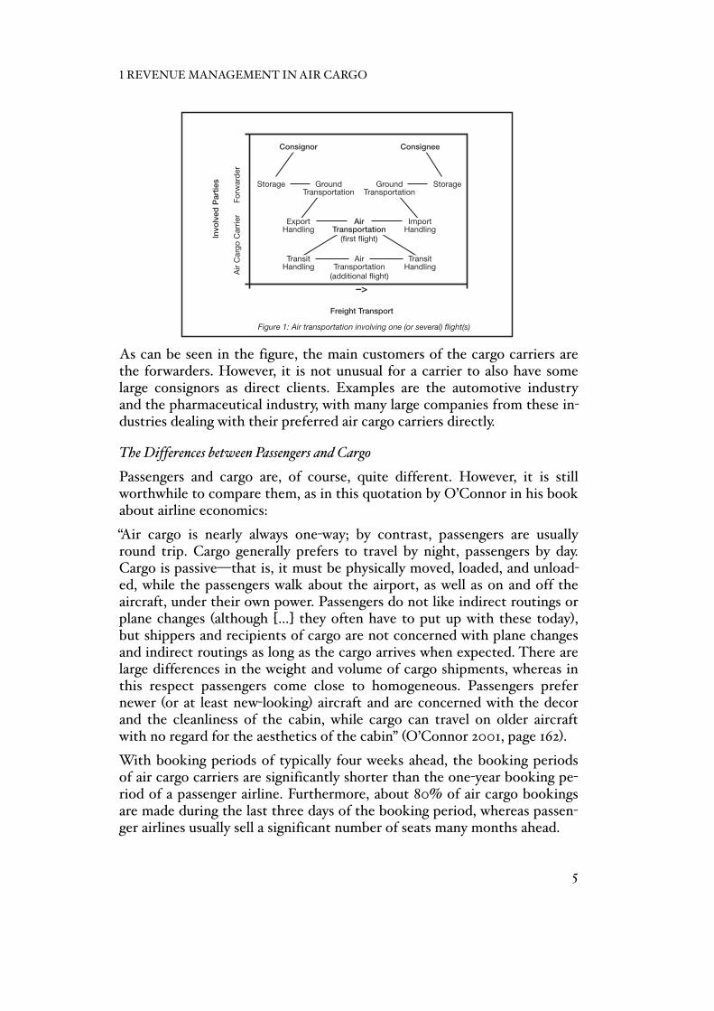
As can be seen in the figure, the main customers of the cargo carriers are the forwarders. However, it is not unusual for a carrier to also have some large consignors as direct clients. Examples are the automotive industry and the pharmaceutical industry, with many large companies from these in-dustries dealing with their preferred air cargo carriers directly.

The Differences between Passengers and Cargo

Passengers and cargo are, of course, quite different. However, it is still worthwhile to compare them, as in this quotation by O’Connor in his book about airline economics:

“Air cargo is nearly always one-way; by contrast, passengers are usually round trip. Cargo generally prefers to travel by night, passengers by day. Cargo is passive—that is, it must be physically moved, loaded, and unload-ed, while the passengers walk about the airport, as well as on and off the aircraft, under their own power. Passengers do not like indirect routings or plane changes (although […] they often have to put up with these today), but shippers and recipients of cargo are not concerned with plane changes and indirect routings as long as the cargo arrives when expected. There are large differences in the weight and volume of cargo shipments, whereas in this respect passengers come close to homogeneous. Passengers prefer newer (or at least new-looking) aircraft and are concerned with the decor and the cleanliness of the cabin, while cargo can travel on older aircraft with no regard for the aesthetics of the cabin” (O’Connor 2001, page 162).

With booking periods of typically four weeks ahead, the booking periods of air cargo carriers are significantly shorter than the one-year booking pe-riod of a passenger airline. Furthermore, about 80% of air cargo bookings are made during the last three days of the booking period, whereas passen-ger airlines usually sell a significant number of seats many months ahead.

over truck on domestic hauls—that international air cargo has shown impressive development despite the cheaper rates by sea” (O’Connor 2001, page 182f.).

Turning to the supply side, an odd feature of the air cargo market is that approximately 50% of the offered cargo capacity is on passenger planes: thus, a large part of the cargo offer derives from passengers travelling on passenger planes since each passenger plane offers a certain amount of cargo capacity (see Holloway 2003, pages 179 and 400).

The Transportation of Air Cargo

A brief overview of the physical transportation of air cargo is given in Figure 1 below, which shows the process of transporting freight over one or more flight legs. The figure also helps explain some of the business terms used in air cargo.

–>

TransitHandling

(additional flight)

(first flight)

AirTransportation

TransitHandling

Figure 1: Air transportation involving one (or several) flight(s)

Freight Transport

Forw

arde

rA

ir C

argo

Car

rier

Invo

lved

Par

ties Ground

TransportationStorage

ImportHandling

GroundTransportation

AirTransportation

ExportHandling

Storage

Consignor Consignee

As can be seen in the figure, the main customers of the cargo carriers are the forwarders. However, it is not unusual for a carrier to also have some large consignors as direct clients. Examples are the automotive industry and the pharmaceutical industry, with many large companies from these industries dealing with their preferred air cargo carriers directly.

The Differences between Passengers and Cargo

Passengers and cargo are, of course, quite different. However, it is still worthwhile to compare them, as in this quote by O’Connor in his book about airline economics:

© 2006 Johannes Blomeyer. All rights reserved. Confidential

June 13, 2006 10!"#$%&'()*(+,%-&.,%#/,(01"(2%3'&$%4

1 REVENUE MANAGEMENT IN AIR CARGO

5

It is also important to note that the ten largest forwarders often generate 70% or more of an air cargo carrier’s business, meaning that an air cargo carrier usually has fewer customers than a passenger airline. Further, the applicable freight rates for the large customers are usually negotiated in advance. The rate between Origin A and Destination B, for example, may be agreed upon at 1.– euro per chargeable kilogram for all bookings by a particular forwarder made within the following three months.

In addition to the above aspects, Holloway noted some further differences between passengers and cargo. According to Holloway (2003, pages 572f.), cargo space is not as ‘fungible’ as a passenger seat (as can be illustrated by heavy shipments that need a specific location within the plane); the car-riage of certain goods is highly regulated (e.g., dangerous goods); and the cargo capacity of a passenger flight (the ‘belly space’) might not be known until very close to departure due to uncertain passenger numbers (‘no-shows’) and unknown baggage figures.

Another difference between passengers and cargo is, according to Herr-mann et al., that low-yield passengers tend to book well in advance, where-as the “excess output of cargo space on many medium- and long-haul routes […] has contributed to the reverse situation where ad hoc late sales are of-ten made at lower-than-contract rates” (see Herrmann et al. 1998; the cita-tion is from Holloway 2003, page 573).

However, passengers and cargo are not completely different, since both have a certain weight and volume, and both can be booked on the same flight (if it is a passenger flight). Both passengers and cargo can be booked in advance, both can be cancelled or might not show up at all, and some-times they share their final destination—as is the case with orchestras and ensembles visiting other countries, since their excess baggage (such as in-struments and sound equipment) is commonly declared and transported not as baggage but as cargo.

The Specifics of Cargo Revenue Management

While Passenger Revenue Management and Cargo Revenue Management share many concepts and ideas (they even share a basic terminology), they are not the same. The major differences are the lumpiness of the cargo demand, the shorter booking period for cargo, the fact that the capacities and the booking requests in air cargo have two dimensions, and the fact that cargo booking requests can cause a substantial amount of stowage loss. However, since the situation with cargo fulfils the general requirements for applying Revenue Management techniques (see Kimes 2001, pages 4ff., for an outline of these requirements, and Hendricks and Elliott (2003) for a discussion on how Cargo Revenue Management is different), an investment in a Cargo Revenue Management System may be sensible—provided that it meets some critical success factors.


6

The Critical Success Factors

One of the most critical success factors is a carrier’s ability to segment the demand according to the customers’ willingness to pay. In cargo, this is remarkably more difficult than on the passenger side because the usual re-strictions used to separate high-yield customers from the low-yield cus-tomers do not hold. There is, for example, no freight ‘under the age of 27’, a ‘Saturday night stay’ does not cause the high-yield freight considerably more discomfort than the low-yield freight, and restrictions requiring the purchase of a return ticket, to give another example, simply do not make sense with cargo.

Hence, segmentation is not easy, and the assumption “that demand for a given [fare] class does not depend on the capacity controls; in particular, [that] it does not depend on the availability of other [fare] classes”, as Tal-luri and van Ryzin put it, is not automatically met. “Its only justification”, they continue, “is if the multiple restrictions associated with each class are so well designed that customers in an upper class will not buy down to a lower class and if the prices are so well separated that customers in a lower class will not buy up to a higher class if the lower class is closed” (Talluri and van Ryzin 2004, page 34).

However, if this assumption is not met, the result is a less than perfect demand segmentation (see Talluri and van Ryzin 2004, page 34); and a less than perfect demand segmentation has, of course, an adverse effect on demand forecasting because buying up—as well as buying down—will result in a different demand than was anticipated in the respective rate classes.

Further, even if a carrier has been successful in segmenting the demand, the demand forecast can still be wrong and, hence, the quality of the demand forecast is critical for the success of any Revenue Management System. This is true for any Revenue Management System, and especially for a Cargo Revenue Management System.

The perceived fairness of a Cargo Revenue Management System is also of great importance since most cargo carriers usually deal with just a few major customers, and they do so on a regular basis. For a further discussion on the subject of perceived fairness in Revenue Management, see Kimes (1994).

Other critical success factors are listed in Hendricks and Elliott (2003) un-der the heading “Challenge Checklists” and in Elliott (2002, pages 11ff.) under the heading “Tactics for Success”.


7

1.2 Literature

An extensive discussion on Revenue Management in general is provided in the book by Talluri and van Ryzin (2004) entitled “The Theory and Prac-tice of Revenue Management”. It does have a section on Cargo Revenue Management but, in comparison with Passenger Revenue Management, this section is small (pages 563-564).

Another influential text on Revenue Management is the Ph.D. thesis by Williamson (1992). This thesis, entitled “Airline Network Seat Inventory Control”, discusses various aspects of managing passenger revenues and is a good introduction to the subject.

The article “Revenue Management and e-Commerce” by Boyd and Bilegan (2003) traces the history of Revenue Management and gives a good over-view of earlier literature on forecasting, optimisation, and control.

The Literature on Cargo Revenue Management

A broad search has revealed that there is little literature specifically on Cargo Revenue Management. The revenue research overview by McGill and van Ryzin (1999), for example, has a bibliography of over 190 refer-ences, but almost all of them refer to Passenger Revenue Management. It is only in the past two or three years that interest in Cargo Revenue Man-agement has risen substantially.

Generally speaking, there are four types of literature on Cargo Revenue Management in the public domain: scientific papers from academia, papers by the vendors of Cargo Revenue Management Systems, reports from practitioners, and published patent applications. In addition to this cargo-specific literature, a number of publications claim that their results can also be applied to cargo.

The major literature that relates to the subject of this dissertation is out-lined below in chronological order.

The article “Air Cargo Revenue Management: Characteristics and Com-plexities” by Raja G. Kasilingam (1996) focuses on the differences between Passenger Revenue Management and Cargo Revenue Management, and discusses “some of the complexities involved in developing and implement-ing [Cargo Revenue Management]” (page 37). Kasilingam also presents a one-dimensional model for overbooking and a one-dimensional model for bucket allocation (a form of booking request control) (pages 41-43).

In his book “Logistics and Transportation: Design and Planning”, Kasil-ingam (1998) wrote about the density of a product (i.e., its volume-to-weight ratio) and about the consequences of density on transportation, storage, and billing (page 25).


8

Kasilingam also noted the importance of grouping products, which “may be done based on their similarity in product characteristics such as weight [and] volume […].” The book has a section about data aggregation, similar-ity measures, and clustering methods (ibid., pages 27 and 29-33). Further-more, it has some information on logistics metrics and notes that it is cru-cial to use the right measurement units (ibid., page 230). Kasilingam also writes about the consolidation business (ibid., page 179), and the contents of his 1996 article are again presented (on pages 189-199). However, most of the book is not sufficiently detailed to capture the specifics of air cargo.

In 1998, in the United States, Talluri filed a patent application entitled “Revenue Management System and Method” (patent number US 6,263,315). The patent concerns multidimensional lookup tables of access price values and, according to Talluri, it has an application in Air Cargo Revenue Man-agement (Talluri 1998, column 10).

Also in 1998, Hamoen published a paper about combination carriers and a dedicated air-cargo hub-and-spoke network (Hamoen 1998). Although this paper is not focused on Cargo Revenue Management, it does contain some interesting information about the economics of air cargo, including net-work types, deregulation, and market segmentation.

Karaesmen’s Ph.D. thesis about Revenue Management also has a chapter on cargo, entitled “Using Bid Prices in Air Cargo Revenue Management”. Karaesmen (2001) claimed on page 4 to “show how a practical airline seat inventory control model can be adapted by air cargo to control both weight and volume capacities.” Furthermore, she claimed that “the model for air cargo requires a continuous linear programming formulation” (ibid., page 4), even though she then went on to refer to the discretisation of the solu-tion space as the most effective way of obtaining numerical results.

The focus of her work, however, was not on finding the best discretisation of the weight and volume space, but to prove, among other things, that “any […] discretization with the same asymptotic property (all regions get smaller in both dimensions […]) can be used” to approximate the infinite dimensional linear programming problem (ibid., page 24; see also pages 23 and 56). Moreover, she claims “that under certain topological conditions, there is no duality gap for our optimization problem [the continuous linear programming formulation]” and that bid prices do exist (ibid., page 23).

It is worth noting that Karaesmen assumed that the revenues from book-ing requests are only a function of their weight and volume (see ibid., page 17), ruling out the possibilities that two booking requests with the same weight and volume could end up being charged at different rates. Hence, Karaesmen did not try to differentiate among the booking requests accord-ing to their rate (at least not beyond their weight and volume consump-tion).


9

The book “An Introduction to Airline Economics” by William E. O’Connor (currently in its sixth edition) has many profound insights into the subject and a dedicated chapter about the economics of air cargo (see O’Connor 2001, pages 153ff.). The chapter about cargo excels in analysing the demand, identifies what drives the supply, and identifies those factors that deter-mine the rates.

In 2001, Gliozzi and Marchetti filed a patent for a “Yield Management Method and System” in Great Britain. This patent application was also filed in the United States under US 2003/0065542 in 2002. In brief, their invention determines “an authorisation to allocate the offered capacity for each capacity variable of each category in the future instance of the service by applying a stochastic model to the historical scenarios according to the corresponding probabilities” (Gliozzi and Marchetti 2003a, page 1). More specifically, they claim to have found an approach that avoids the need for a demand classification by using the original request data and having these sent directly to the optimisation model using multiple stochastic scenarios.

A paper by Gliozzi and Marchetti, entitled “A New Yield Management Ap-proach for Continuous Multi-Variable Bookings: The Airline Cargo Case”, concerns the implementation of a complete Cargo Revenue Management System (Cargo RMS) that was “going to be fully operational in 2002 at a ma-jor European airline” (Gliozzi and Marchetti 2003b, page 386). The paper describes various aspects of managing revenue in air cargo (including the existence of a density mix; ibid., pages 380-381), and emphasises that “both the variables [i.e., the weight and the volume] have to be treated symmetri-cally and at the same level in the definition of the models” (ibid., page 372). Their “New Yield Management Approach for Continuous Multi-Variable Bookings” is based on the 2001 patent application “Yield Management Method and System” by Gliozzi and Marchetti (2003a).

An excellent chapter about the economics of airfreight can be found in Doganis’ book “Flying Off Course” (Doganis 2002). In this chapter, the demand for airfreight services is analysed by considering, for example, the demand for emergency freight, such as spare parts for machinery; the de-mand for legal papers and artwork; the demand for transporting valuables, such as gold and jewellery (because of the added security); the demand for transporting perishables, and, of course, the demand for transporting ‘regu-lar’ freight (ibid., pages 300ff.). Further, the book has a chapter on the eco-nomics of supply and another about the pricing of airfreight.

In the same year, Radnoti published his book “Profit Strategies for Air Transportation” (Radnoti 2002). The book gives a broad overview of vari-ous aspects of air transportation and does not shy away from cargo, even though some of the presented data appeared to be obsolete (they were from the 1960s and 1970s). Still, the book has a hands-on approach and provides many insights into the subject.


10

A 2002 paper by Elliott provides some background information on the eco-nomic trends in air cargo and recommends basing Cargo Revenue Manage-ment on three “strategic realities”. Strategic reality #1 is (according to Elli-ott) that “Revenue Management is an ongoing business function”, strategic reality #2 is that “Revenue Management helps manage the crisis”, and stra-tegic reality #3 is that “Revenue Management opportunities can still be found, even in a depressed market” (see Elliott 2002, pages 7ff.).

The book “Straight and Level: Practical Airline Economics” by Holloway (2003), another book about airline economics, not only has a chapter about Revenue Management but also gives some information concerning how to manage freight revenues.

In 2003, Hendricks and Elliott put a short paper titled “Implementing Rev-enue Management Techniques in an Air Cargo Environment” on the Inter-net. The paper is clearly written, and it “reviews the techniques of Revenue Management and how they relate to the specific nature of the Air Cargo Business” (Hendricks and Elliott 2003, page 1).

The paper “Securing the Future of Cargo”, from the series “Mercer on Travel and Transport”, provides some useful information on why only a few carriers use a Cargo Revenue Management System (Kadar and Larew 2003). On page 5 of the paper, the authors, Kadar and Larew, summarise that “cargo capacity is volatile”, that “cargo demand is multidimensional”, that “cargo customers are concentrated”, and that the “returns on investments are lower for air cargo carriers [than for passenger airlines]” because the cargo carriers are usually smaller in size.

The paper “On an Experimental Algorithm for Revenue Management for Cargo Airlines” by Bartodziej and Derigs (2004) is about an itinerary-based network model that not only considers the routing options in air cargo, but is also able to calculate the bid price of a booking request (pages 60-64).

Slager and Kapteijns wrote a practice paper in 2004 entitled “Implementa-tion of Cargo Revenue Management at KLM”. The paper describes the con-cept and the implementation of a new Cargo Revenue Management System at KLM Airlines after a failed attempt that “had focussed too much on IT and a scientific approach” (Slager and Kapteijns 2004, page 82). The new approach seems to centre on the setting of so-called Shipment Entry Con-ditions (SEC). “The SEC”, they wrote on page 86, “can be set per cubic metre for volume constrained flights, or per kilo for payload restricted flights” but, unfortunately, the paper has no information on how to deal with flights that are expected to be restricted in both weight and volume. Their paper also failed to mention instruments that are available to increase the cargo revenue of a flight, beyond to “protect high margin cargo, on top of eliminating low margin cargo” (ibid., page 90). Additional information on Revenue Management at KLM Cargo can be found in Couzy (2004).


11

In their paper “Fleeting with Passenger and Cargo Origin-Destination Booking Control”, Klabjan and Sandhu (2005) compare Passenger Revenue Management and Cargo Revenue Management, and present a so-called Cargo Mix Bid Price Model. Among other topics (which are only loosely connected to cargo), they focus on the possibility of transporting cargo via different routings (ibid., pages 6ff.). An earlier presentation of their ap-proach was given in Klabjan and Sandhu (2004).

Cooper et al. (2005) model the Cargo Revenue Management problem as a Markov Decision Process and explicitly take into account that the volume of a booking request is, in practice, a random variable because its value “is learned only just before the flight’s departure” (ibid., page 1). They pub-lished a revised version of their paper in 2006 (Cooper et al. 2006).

In the last chapter of his 2005 Ph.D. thesis “Revenue Management: New Features and Models”, Pak presented his approach for managing revenue from air cargo under the title “Bid Prices for a 0–1 Multi Knapsack Prob-lem”. This approach claims—not unlike the one by Gliozzi and Marchetti —to “treat the cargo shipments as the unique items that they are” (Pak 2005, page 9). According to Pak, “the weight, volume and profit of each booking request [per kilogram] are random and continuous variables” (ibid., page 111), and “the fundamental difference between Cargo and Pas-senger Revenue Management, is that cargo shipments are uniquely defined by their profit, weight and volume whereas passengers generally belong to one of a limited number of price classes” (ibid., page 141). He also states that “profit, weight and volume are related to each other since they all re-flect the size of the shipment” (ibid., page 128), but does not elaborate on what is meant by the size of a shipment, if not its weight. An earlier version of Pak’s work was published in 2004 (Pak and Dekker 2004).

Although the paper “Profit Maximization in Air Cargo Overbooking” by Cakanyildirim and Moussawi (2005) is mostly about overbooking, they do include some basic cargo definitions, as, for example, the definition of the density of a piece of cargo, as well as a definition of its chargeable weight. They also mention the phenomenon that is elsewhere known as the density mix (ibid., pages 6-10).

One of the more recent papers about Cargo Revenue Management is by Huang and Hsu (2005), entitled “Revenue Management for Air Cargo Space with Supply Uncertainty”. This paper takes into account the supply uncertainty of available air cargo space on a flight and the incurred penalty for denied boarding (in the air cargo industry, the term ‘denied boarding’ is known as ‘offloads’), but their dynamic programming model is one-dimen-sional, based on weight.


12

They are aware of the business practice of selling chargeable weight, but their statement is that airlines sell cargo space in terms of tonnes or kilo-grams and that the “airlines are not sure that the aircraft can handle the shipments for the space sold” (Huang and Hsu 2005, page 572).

Other papers include those by Bazaraa et al. (2001: a general overview of Cargo Management), Chew et al. (2002: Cargo Revenue Management from the perspective of the forwarder), Feller (2002: Revenue Management as a Dynamic Stochastic Knapsack Problem with multidimensional resources), and Billings et al. (2003: a discussion of various aspects of Cargo Revenue Management). The paper by Gallego and Phillips (2004) about the Revenue Management of flexible products also claims to have applications in air cargo. Further papers include those by Chen et al. (2003: about Cargo Rev-enue Management and routing), Kimms and Müller-Bungart (2004: an arti-cle about the construction of multidimensional booking classes), Naraya-nan (2004: a presentation mainly about the Bayesian forecasting of cargo demand), and Derigs et al. (2006; another paper about Revenue Manage-ment and routing).

The Publications by the Author on the Subject

In 1999, my first thoughts on the subject of Cargo Revenue Management were documented in an unpublished working paper (“for internal use only”) by Lufthansa Cargo. In this paper, the instruments that are available to in-crease the revenue of a flight are described as the rate mix, the load mix, overbooking, pre-flying shipments, rebooking shipments, and short-term capacity adjustments (Blomeyer 1999, page 5).

Further publications have included several patent applications. The results of this dissertation have fed into German patent application DE 10 2004 023 833.2 (priority date 13.05.2004), European patent application EP 1 596 317 A1 (publication date 16.11.2005), and United States patent application US 2006 001 5396 A1 (publication date 19.1.2006).


13


14

2 Preliminary Notes

This chapter has two sections. The first is about the general notation used, and the second section is more specific concerning quantity units and value ranges.

2.1 Notation

The names of the variables, parameters, and constants are case-sensitive and their meaning may depend on the subscript. R, for example, is the rev-enue, r is a rate, and rb is the rate of the booking request b. Furthermore, the concepts can play different roles in various parts of the dissertation. Flight revenue, for example, is mostly treated as a variable, but in the chap-ter about booking request control with stowage loss, flight revenue is used as a parameter. The role of the symbols should, however, be clear within their context.

Units, where applicable, are given in brackets, and the term [unitless] indi-cates that a value has no units.

2.2 Primary and Secondary Units

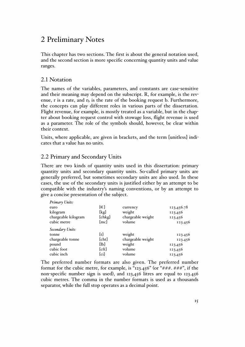
There are two kinds of quantity units used in this dissertation: primary quantity units and secondary quantity units. So-called primary units are generally preferred, but sometimes secondary units are also used. In these cases, the use of the secondary units is justified either by an attempt to be compatible with the industry’s naming conventions, or by an attempt to give a concise presentation of the subject.

Primary Units:euro+ + + + [€]+ + currency+ + + 123,456.78kilogram+ + + [kg]+ + weight++ + + 123,456chargeable kilogram+ + [chkg]++ chargeable weight+ + 123,456cubic metre + + + [mc]+ + volume+ + + 123.456

Secondary Units:tonne+ + + + [t]+ + weight++ + + 123.456chargeable tonne+ + [cht]+ + chargeable weight+ + 123.456pound+ + + + [lb]+ + weight++ + + 123,456cubic foot+ + + [cft]+ + volume+ + + 123,456cubic inch+ + + [ci]+ + volume+ + + 123,456

The preferred number formats are also given. The preferred number format for the cubic metre, for example, is “123.456” (or “###. ###”, if the non-specific number sign is used), and 123,456 litres are equal to 123.456 cubic metres. The comma in the number formats is used as a thousands separator, while the full stop operates as a decimal point.

15

If the decimals of a number are suppressed, the number has a decimal point but no decimals (e.g., “123.”). This number format is mainly used in illustra-tions to save space. Another sign used to save space is the double tilde which denotes an approximate value (e.g., π ≈ 3.14). Finally, a dash, as in “123.– euro”, replaces the zeros after the decimal point.

Please note that the term [mc] has been chosen as an abbreviation for the cubic metre to avoid confusion with the term [cm] used for centimetres. The format [m3] is inconvenient because of its superscript, and the term ‘m3’ could be misleading if it is used as a prefix: m3 45, for example, could be easily read as either 45 cubic metres or 345 metres.

The Date and Time Format

The preferred date and time formats are day.month.year and hour:minute, as in 31.12.2003 and 12:34.

The Rounding Rules

Aside from the preferred formatting, it would be prudent to explain any rounding rules used in the air cargo industry. Reasons for using a rounding rule might be, for instance, a legal requirement, a prevalent business prac-tice, an attempt to achieve numerical stability, or an attempt to simplify the reading of a number. To give an example, a simple rounding rule, which is based on a prevalent business practice, will be presented below.

In air cargo, the chargeable weights of bookings and booking requests are rounded up to the next half chargeable kilogram (see IATA Resolution 502). A chargeable weight of 100.1 chargeable kilograms, for example, will be rounded up to 100.5 chargeable kilograms, while a chargeable weight of 100.6 chargeable kilograms will be rounded to 101 chargeable kilograms. Accordingly, the formula for calculating the rounded chargeable weight is 0.5 2 chargeable weight.

Despite their importance in the specification of a real-world Cargo Reve-nue Management System, rounding rules are not further considered in this dissertation because they are beyond the scope of this dissertation.

The Conversion Rules

To convert primary units into secondary units (and vice versa), several con-version constants are needed. The tonne conversion constant is used to change tonnes into kilograms, and the chargeable tonne conversion con-stant changes chargeable tonnes into chargeable kilograms. Both constants are formally introduced below.

Tonne and Chargeable Tonne Conversion Constants:tc + 1,000 [kg/t]+ + tonne conversion constantchtc+ 1,000 [chkg/cht]+ chargeable tonne conversion constant


16

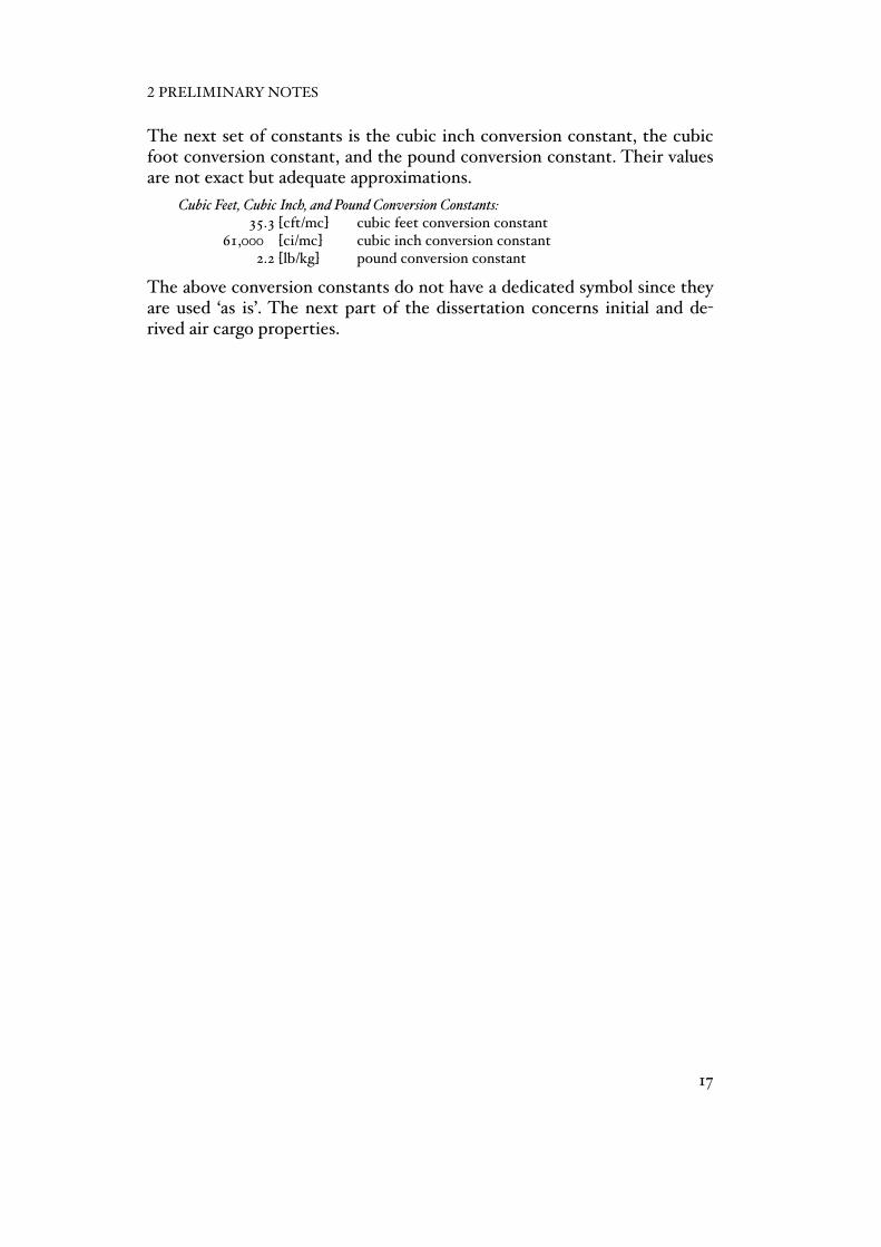
The next set of constants is the cubic inch conversion constant, the cubic foot conversion constant, and the pound conversion constant. Their values are not exact but adequate approximations.

Cubic Feet, Cubic Inch, and Pound Conversion Constants: 35.3 [cft/mc]+ cubic feet conversion constant 61,000 [ci/mc]+ cubic inch conversion constant 2.2 [lb/kg]+ pound conversion constant

The above conversion constants do not have a dedicated symbol since they are used ‘as is’. The next part of the dissertation concerns initial and de-rived air cargo properties.

2 PRELIMINARY NOTES

17

PART II: AIR CARGO PROPERTIES

3 Initial and Derived Properties in Air Cargo

Managing revenue in air cargo is primarily a matter of confirming the ‘ad-vantageous’ booking requests and rejecting the ‘disadvantageous’ ones. How this should be done will be the subject of a later chapter but, clearly, any plan to control the confirmation of a booking request has to do with its initial air cargo properties. The initial air cargo properties are the weight, the volume, and the revenue of an item. The initial air cargo properties are accompanied by so-called derived air cargo properties. Derived air cargo properties are, for example, not only the density of an item and its charge-able weight, but also the weight and volume coefficients of the chargeable weight, as well as its rate. Later in the chapter, a simple set of derived air cargo properties will be presented, and this simple set will then be com-pared with an extended set. The chapter concludes with a consideration of the contribution made to the field.

3.1 Weight, Volume, and Revenue

The weight and volume of bookings, booking requests, and flight capacities are typically expressed in kilograms and cubic metres, or [kg] and [mc], while the revenue of bookings and booking requests is typically expressed in euro, or [€].

The weight, the volume, and the revenue are considered to be initial air cargo properties because they are real quantities in air cargo. The symbols and value ranges of these initial air cargo properties are stated below.

Weight, Volume, and Revenue:W+ [0, ∞) [kg]+ + weightV+ [0, ∞) [mc]+ + volumeR+ [0, ∞) [€]+ + revenue

All quantities have a lower bound of zero because there is no reason, as yet, to believe that negative weight, volume, or revenue quantities make any sense. The given value ranges do not, however, take account of any specific limitations, as, for example, the payload restrictions of an airplane. In the next section, some derived air cargo properties are introduced.

3.2 Density, Standard Density, and Chargeable Weight

The most important derived air cargo properties are the density and the chargeable weight of a piece of freight (or of any other item which has a weight and volume). Both quantities are considered to be derived since they are calculated from the initial air cargo properties of weight and volume. Despite its status of being ‘derived’, the density is a well-known and well-established figure for describing the volume-to-weight ratio of

19

bookings and booking requests in air cargo. The chargeable weight is also well-known in air cargo, but only implicitly and not as an explicit figure. This is because the chargeable weight is the greater of two figures, namely the actual weight and the volume weight. If the volume weight is higher than the actual weight, the volume weight simply replaces the actual weight in certain calculations (for example in the calculation of the booking re-quest’s rate; see www.tci-transport.fr/volum_uk.htm). Prior to discussing the chargeable weight, however, the density and the standard density will be considered.

The Density

The cargo density reflects the bulkiness of an item with bulky items having large volumes per weight, whereas items which are comparatively dense have less volume than one might expect for their weight.

Contrary to the definition of density in physics, the density in air cargo is defined as ‘volume divided by weight’.

Definition of the Density in Air Cargo:d = 1,000 V/W

The conventional unit of density in air cargo is cubic metres per tonne, the symbol is d, and the value ranges from ‘pure weight’, with a density of zero, to ‘pure volume’, with a density of infinity.

Density:d+ [0, ∞] [mc/t]+ + density

Even though the above density definition is perfectly adequate for many calculations, it cannot deal with items that have zero weight. In other words, the density definition must be modified to be able to calculate a density for items (or entities) that have zero weight, and this is achieved by stating that the combination of positive volume and zero weight equates to an infinite density. Items (or entities, for that matter) with zero or infinite densities are, incidentally, not uncommon in air cargo. The bookable flight capacities at departure, for example, are often zero in weight or in volume. Booking updates, which are another entity used in air cargo, can have a zero or an infinite density if only additional weight or additional volume is being requested.

However, there are entities in air cargo that may have no defined density at all. If, for example, the remaining weight and volume capacities of a flight are both zero, the density of the bookable capacity is, in fact, indeter-minate.

By being able to deal with entities that have a positive volume but zero weight, the generic density definition overcomes the arbitrariness of using an entity’s volume divided by its weight as a measure of its density. To be specific, a density which is calculated as a volume divided by a weight will


20

be indeterminate for a zero weight, and the more conventional density, which is calculated as a weight divided by a volume, is indeterminate for a zero volume. However, although the first fraction can handle the zero vol-ume case and the second fraction can handle the zero weight case, neither fraction can handle both. Therefore, there is a fundamental need to define density in air cargo generically and so avoid the necessity of having to work with two definitions. If the density in air cargo is defined generically, it no longer matters whether the density is expressed as a volume divided by its weight, or as a weight divided by its volume. A generic density definition of the volume-divided-by-weight type is given below.

Density as a Function of Weight and Volume:if+ W = 0 and V = 0+ then d is indeterminateelseif+ W > 0 and V ≥ 0+ then d = (V/W) tcelseif+ W = 0 and V > 0+ then d = ∞

As can be seen, the generic density definition makes use of the tonne con-version constant to achieve unit consistency.

It should be noted that the actual density values are rarely affected by the limits placed on weight and volume value ranges. This is because the den-sity is a fraction, and neither the limited value range for the nominator of that fraction, nor the limited value range for its denominator, necessarily lead to a limited density value range. In the world of air cargo, the density range of an item is probably more often restricted by the physical limits on the density itself. Real freight, for example, cannot have a zero density be-cause any tangible cargo has at least some volume and, for a similar reason, it is very unlikely that a physical piece of cargo has an infinite density.

The Standard Density

The standard density is a very important figure in air cargo because it is used for the calculation of the chargeable weight of freight, and the freight’s chargeable weight, in turn, is the basis for the revenue the carrier aims to earn. Although the value of the standard density is, at least in prin-ciple, negotiable, all airlines which are members of the International Air Transport Association (IATA) have agreed on a common value.

Physically, the standard density refers to what is considered as the average density of regular freight. As such, the standard density has not only an ef-fect on the calculation of the freight’s chargeable weight but also on nearly all other aspects of managing and transporting freight in the air cargo in-dustry. The optimum volume-to-weight ratio of the cargo hold of commer-cial cargo airplanes, for example, is similar to the volume-to-weight ratio of the standard density in order to maximise freight carrying opportunities.

Further elaborating on the subject, O’Connor refers to planes that have been designed to be freighters from the drawing board onwards as ‘dedi-cated’ or ‘uncompromised’ cargo aircraft (O’Connor 2001, page 162).

3 INITIAL AND DERIVED PROPERTIES IN AIR CARGO

21

Dedicated freighters differ significantly from freighters that were conver-ted from passenger use or were made at the factory as freighters but using the basic designs of a passenger aircraft because “an aircraft whose initial design was premised on the requirements of passenger service will, when used as a freighter, usually become filled to capacity with respect to space well before the maximum permissible payload weight is reached”, while a dedicated cargo aircraft “should be designed to reflect the usual trade-off between cube [i.e., the volume] and the weight of the cargo that travels in major markets” (ibid., pages 162f.). More information about this subject can be found in Holloway (2003, pages 500f.), Roskam (1989, pages 76ff.) and Wood et al. (2002, page 192).

Besides serving as a guideline in the design of an uncompromised cargo air-craft, the IATA Interline & Revenue Management Services Newsletter (2003, page 14) provides an additional reason why it is important to have a standard density: “… it facilitates the design and the production of standard aircraft containers, pallets and handling equipment, simplifying the move-ment of shipments from one aircraft type to another, and from one airline to another.”

The symbol for the standard density is sdc, and its value is 6 cubic metres per tonne as formally defined below.

IATA Standard Density:sdc+ 6 [mc/t]+ + standard density constant

If the IATA standard density were to be expressed as an inverse (i.e., con-ventional) density in pounds per cubic inch, its value would be approxi-mately 0.006 [lb/ci], while if the standard density were to be expressed as an inverse density in pounds per cubic feet, its value would be approxi-mately 10.4 [lb/cft].

The aforementioned value of 6 cubic metres per tonne has been valid since October 1981; prior to that date, the IATA standard density was 7 cubic metres per tonne. In May 2002, the IATA Composite Cargo Tariff Co-ordinating Committee suggested changing the standard density from 6 cubic metres per tonne to 5 cubic metres per tonne (see the Composite Resolution 502 from the IATA Composite Cargo Tariff Co-ordinating Committee 2002) in order to “incite improvements in the efficiency of packaging methods to reduce the volume of their shipments using more compact […] packaging” because “this would allow airlines to increase ca-pacity with only a marginal increase in operating costs” (IATA Press Release Low Density Cargo March 2005, page 1).

Another reason that an update to the standard density was proposed was that “aircraft performance has improved significantly in the 20 years since this standard was last changed—with more powerful engines able to lift more weight, while the space available in the cargo hold has remained


22

static”, so that many flights “cube out” before they “weigh out” (ibid., page 1). However, Composite Resolution 502 was withdrawn at the Special Composite Cargo Conference in 2005 and never implemented (see IATA 2005, page 1).

Also mentioned in the initial resolution was the fact that the types and overall nature of air cargo have changed. “In the past, air cargo contained heavy machinery and similar commodities and these have been replaced by high-technology products such as computers, software […] and other elec-tronic equipment. Virtually none of these products existed when the first Boeing 747 entered service over 32 years ago. These goods are typically lighter, but are higher in value than most items traditionally shipped by air in the past” (IATA Press Release Low Density Cargo March 2005, page 1). Hence, there is a mismatch between the possibility of lifting more weight and the need to accommodate more volume.

More information about the recent developments in the density of freight can be found in Sulogtra (2002). For a detailed discussion on the motives and consequences of a standard density change, see ACCC (2004). However, for the time being, the value of the standard density remains 6 cubic me-tres per tonne.

Although this value is assumed throughout the dissertation, great care has been taken to make a distinction between the standard density function and its actual value so as to be able to handle future changes without any difficulties. In comparison, the standard densities in sea and road cargo are currently 1 and 3 cubic metres per tonne respectively.

Densities below the standard density are referred to as high densities (even though the numerical values are lower), and densities above the standard density are called low densities (even though the numerical values are higher). Simply put, high-density items are comparatively heavy, and low-density items are comparatively bulky. The explicit definition of what are considered as high, standard and low densities in air cargo is given below.

High, Standard, and Low Densities in Air Cargo:if+ 0 ≤ d < sdc+ + then d is a high densityelseif+ d = sdc+ + then d is a standard densityelseif+ sdc < d ≤ ∞+ + then d is a low density

Typical density figures for various goods are given in Wood et al. (2002) on page 192.


23

For practical purposes, it is useful to further classify these densities into smaller subgroups. A classification with three subgroups for the high-density category and three subgroups for the low-density category is suggested below.

Moderate, Medium, and Extreme Densities in Air Cargo:if+ 0 ≤ d < 2.4+ + then d is an extremely high densityelseif+ 2.4 ≤ d < 4.8+ + then d is a medium high densityelseif+ 4.8 ≤ d < 6+ + then d is a moderately high densityelseif+ d = 6+ + + then d is a standard densityelseif+ 6 < d ≤ 7.5+ + then d is a moderately low densityelseif+ 7.5 < d ≤ 15+ + then d is a medium low densityelseif+ 15 < d ≤ ∞+ + then d is an extremely low density

Even though this classification might look somewhat arbitrary, it is not. Rather, the density classification is based on the unified density. Unified density is a concept which will be explained in Chapter 5 and, as a result of having based the density classification on the unified density, each high-density subgroup is as extreme, medium or moderate as its counterpart among the low-density subgroups (and vice versa). Furthermore, the sug-gested classification is symmetric and centred around the standard density of 6 cubic metres per tonne.

An illustrated example of different densities, including several extremely high densities, one moderately high density, the standard density, and one extremely low density, is given in Figure 2. The figure shows the weight and volume combinations of the following densities (from left to right): ∞, 4, 2, 1.33, 1, 0.8, 0.66, and 0 [mc/t]. The standard density, of 6 cubic metres per tonne, is shown as a dashed line.

According to the definitions of high, standard, and low densities, any com-bination of weight and volume that is located to the left of the standard density line in Figure 2 has a low density, while all combinations of weight

u > 0ij x > 0ij

XVIII

Complementary Slackness Condition

Com

plem

enta

ry S

lack

ness

Con

ditio

n

(Un)profitability and demand selection

u = 0ij

s > 0ij p = 0ij

u = 0ijs = 0ij

p > 0ij

x = 0ijp = 0ij

p = 0iju =ij

x = 0ij

ijijp = 0 ! x

ijijp = x = 0

u = 0 ! sijij

u = s = 0ijiju " 0 = sijij

u " 0 < sijij

x =ij Dij

0 ! x !ij Dij

Booking class sizes as a function of the booking class rate

0 10 20 30 40 6050

4.00

3.50

3.00

2.50

2.00

0.50

1.50

1.00

0.00

Supply and Demand [cht]

Rat

e [e

uro/

chkg

]Wk

demandforecast

lumpy bid price rate

BCxBCx

Booking class rates as a function of the booking class demand

0 10 20 30 40 6050

4.00

3.50

3.00

2.50

2.00

0.50

1.50

1.00

0.00


Rat

e [e

uro/

chkg

]

Wk

demandforecast


BCoptr

minBCr

BCr

WkBCD– BCw

optmax

0 1 2 43 65

4

3

2

1

0

Weight [t]

Volu

me

[mc]

Figure 2: Weight, volume, and density

# m

c/t

4 m

c/t

2 m

c/t

1.33

mc/

t

1 mc/

t

0.8 mc/t

0 mc/t

0.66 mc/t

1)

stan

dard

den

sity

(das

hed)

: 6 c

ubic

met

res

per t

onne

1)

Figure 22: Rate-graph of a segment

0 20 40 60 80 120100

4.00

3.50

3.00

2.50

2.00

0.50

1.50

1.00

0.00

Chargeable Weight [cht]

Rat

e [€

/chk

g]

–> derivedinitial

Figure 20: Various densities and the extended set

Properties

Varia

ble

revenue[€]

revenue[€]

chargeableweight[chkg]

volume[mc]

weight[kg]

revenue[€]

weightcoefficient

[chkg/chkg]


rate[€/chkg]

volumecoefficient

[chkg/chkg]

unified density[unitless]

weight[kg]

0 100 200 400300 500

400

300

200

100

0

Chargeable Weight [chkg]

Rev

enue

[€]

600

Figure 10: Minimum revenue and chargeable weight breakpoints

100r

500+r

500r

R

Density [mc/t]

Rat

e [€

/chk

g]

Figure 25: Booking requests, a rate-density domain, and its gravity center

s

disl dis

u

risu

risl

domaindemandqis

i

disdomaindensity

risdomain

ratex

x

x

x

x

x x

xx

x

x

density[mc/t]

volume[mc]

m

np

u

NW(s, x) NE(s, u)

SW(p, x) SE(p, u)

D =ij 0x =ij

m

ijijp " 0 = xn

ijijp " 0 ! x ijijp " 0 ! u

nn

s>=0

s=0

u>=0


24

and volume that are located to the right of the standard density line have a high density. Infinite densities are located on the ordinate of the graph, zero densities are located on its abscissa, and the zero weight / zero volume combination is located at the graph’s origin. From the meeting of the density lines, it is clear that the zero weight / zero volume combination can have any density, and hence it does make sense to say that the density of the zero weight / zero volume combination is indeterminate.

The Chargeable Weight

The chargeable weight of freight is also known as its billable or dimen-sional weight. The symbol for chargeable weight is cw, and its unit is the chargeable kilogram. The chargeable weight and its quantity unit are speci-fied below.

Chargeable Weight:cw+ [0, ∞) [chkg]+ + chargeable weight

The value range for the chargeable weight goes from zero chargeable kilo-grams to, strictly speaking, less than infinite chargeable kilograms. It may be possible to tighten this value range by taking the particular context of an item into consideration but, more likely, the value range of the chargeable weight will be restricted by certain weight and volume limits.

Without invoking a dedicated chargeable weight unit (and, in fact, without bothering about the units at all), the chargeable weight is the maximum of an item’s actual weight and its volume divided by the standard density. For generic usage, however, this definition is enhanced by using explicit weight-ing factors for weight and volume (instead of using only the standard den-sity), and by using real units (instead of not using units at all). The result, a generic definition of chargeable weight, is given below.

Chargeable Weight as a Function of Weight and Volume:cw = max {W/wc, (V/vc) chtc}

The generic chargeable weight definition uses three constants: the charge-able tonne conversion constant chtc, the weight constant wc, and the vol-ume constant vc. The chargeable tonne conversion constant has a value of 1,000 chargeable kilograms per chargeable tonne and is only used to achieve unit consistency. The weight constant has a value of 1 kilogram per chargeable kilogram and is used to indicate how many kilograms of pure weight can be tendered for each chargeable kilogram, while the volume constant has a value of 6 cubic metres per chargeable tonne and is used to indicate how many litres of pure volume can be tendered for each charge-able kilogram. Hence, the weight and volume constants form the upper bounds of how many kilograms and litres are allowed in one chargeable kilogram. The weight and volume constants are formally introduced on the next page.


25

Weight and Volume Constants for the IATA Standard Density:wc+ 1 [kg/chkg]+ weight constantvc + 6 [mc/cht]+ volume constant

Although the standard density can be derived from the weight and volume constants by means of simple division, the weight and volume constants cannot be derived solely from the standard density. This is because the weight and volume constants have not only to relate to each other but also to the chargeable weight. In other words, the weight and volume constants are the weight and volume weighting factors in calculating an item’s charge-able weight and, even though there may be many weight and volume con-stants with a volume-to-weight ratio equal to the standard density, there is only one set of weight and volume constants that has volume-to-chargeable weight and weight-to-chargeable weight ratios that match the definition of chargeable weight.

The use of the weight and volume constants not only has the advantage that the weighting factors are now readily available, it also has the benefit that the weight and volume constants can be used independently, as in the generic definition of the chargeable weight above.

Essentially, the purpose of computing the chargeable weight of freight is to marry the weight of an item with its volume to create a broader basis for revenue calculation. If the revenue calculation were based on weight or vol-ume alone, either low-density freight or high-density freight would be un-fairly penalised. O’Connor describes chargeable weight as “the dimensional weight policy of an airline” (O’Connor 2001, page 191). He continues: “For articles of very low density, such as cut flowers and empty plastic bottles, the carriers assume a weight higher than the actual weight and compute the rate on that presumed higher weight. That is, the cube [i.e., the volume] of the shipment is measured, and what is really a fictitious weight is used when looking up the rate in the general commodity rate schedule” (ibid., page 191; see also Holloway 2003, page 142).

The chargeable weight of an item can also be used as a proxy for its size. Furthermore, the demand for transporting items can be measured in terms of their chargeable weights.

To illustrate the concept of chargeable weight, Figure 3 gives some weight and volume combinations which lead to the same chargeable weight. One hundred chargeable kilograms, for example, could be 100 kilograms with a volume up to 0.6 cubic metres, or 0.6 cubic metres with any weight up to 100 kilograms.


26

Although the main reason for computing chargeable weight is to have a comprehensive basis for calculating revenue, the chargeable weight offers more: it is a universal economic term, it can be used to reduce the number of different units, and it has a favourable dimensional scaling.

Since these features of the chargeable weight are somewhat complex, they are discussed in more detail below.

❖ Chargeable weight is a universal economic term.

To prepare the discussion on this feature, some background infor-mation on the use of the chargeable weight in practice will first be considered. Commonly, chargeable weight is only calculated for bookings and booking requests, and not for flight capacities. In other words, the demand of a customer is stated as a request for a charge-able weight with a certain density, whereas the supply of the air cargo carrier is stated as an available weight and volume. These values, i.e., of supply and demand as well as the weights and the volumes, cannot be directly compared since they have different units.

Fortunately, and this is the point where the chargeable weight steps in as a universal economic term, the chargeable weight can be also used to describe the space offered by an air cargo carrier. More specifically, the flight capacities, which are usually expressed in weight and volume units, can be transformed into a product offer with an economic unit. Thus, the available weight capacity of a flight will be converted into a chargeable weight offer that has a zero density, and the available volume capacity will be converted into a chargeable weight offer that has an infinite density.

XII

0 10 20 4030 6050

10000

7500

5000

2500

0

Volume [mc]

Wei

ght [

kg]

Weight, volume and chargeable weight (6:1)

2000

1000

3000

4000

5000

6000

7000

8000

9000

Chargeable Weight [chkg] 6:1

0 10 20 4030 6050

10000

7500

5000

2500

0

Volume [mc]

Wei

ght [

kg]


2000

1000

3000

4000

5000

6000

7000

8000

9000

Chargeable Weight [chkg] 5:1 6:1

0 10 20 4030 6050

10000

7500

5000

2500

0

Volume [mc]

Wei

ght [

kg]

Volume critical due to Low Density Booking Requests

d = 83333 chkg

•

d = 22500 chkg

•

•••• Low

DensityBookingRequests

6:1

0 10 20 4030 6050

10000

7500

5000

2500

0

Volume [mc]

Wei

ght [

kg]

Volume critical due to High Density Capacity

d = 83333 chkg

•

d = 22500 chkg

•

•••• Low

DensityBookingRequests

6:1

High DensityBooking Requests

•

0

High DensityBooking Requests

••••

6:1 4:1

0 2 4 86 …10

4.00

3.00

2.00

1.00

Density [mc/ton]

Rat

e [e

uro/

chkg

]

Rate increase due to a change of standard density

0.00

3:1 4:1 5:1 6:10%

50%

100%

150%

200%

Cha

rgea

ble

Wei

ght [

chkg

]

10000

7500

5000

2500

0

Volume [mc]


010

20

4030

6050

Weight [kg]

1000

0

7500

5000

2500 0

6:1

0 1 2 43 65

4

3

2

1

0

Weight [t]

Volu

me

[mc]

Figure 3: Weight, volume, and chargeable weight

600 chkg

500 chkg

1)

stan

dard

den

sity

: 6 c

ubic

met

res

per t

onne

1)

400 chkg

300 chkg

200 chkg

100 chkg


27

From this point of view, a customer is not buying a certain weight and volume but a bundle of two different goods, namely some chargeable weight that has a zero density and some chargeable weight that has an infinite density. Rather, the air cargo carrier is not offering mere capacities but some marketable products. Flight capacities of, say, 50 tonnes and 600 cubic metres can be sold as 50,000 chargeable kilograms that have a zero density and as 100,000 chargeable kilograms that have an infinite density (in practice, however, they are sold together).

Having restated the supply in terms of chargeable kilograms, the weight supply can be compared with the volume supply, and both can be compared with the demand. As an example, we will consider the demands of two booking requests of 1,000 and 3,000 chargeable kilograms with densities of 4 and 9 cubic metres per tonne respectively. Clearly, in terms of chargeable kilograms, the demand of the second booking request is three times higher thanthe demand of the first booking request. Now, if the first booking request is confirmed, it will use 1,000 chargeable kilograms of the zero-density supply and 666 chargeable kilograms of the infinite- density supply, while the second booking request, if confirmed, will use 2,000 chargeable kilograms of the zero-density supply and 3,000 chargeable kilograms of the infinite-density supply. Hence, the volume consumption of the second booking request is three times greater than the weight consumption of the first booking request, and if both requests are confirmed, the remaining weight and volume supply will be 47,000 and 96,334 chargeable kilograms, respectively. In other words, the remaining volume supply will be more than twice as high as the remaining weight supply.

It might be argued that a chargeable kilogram of pure weight (i.e., a chargeable kilogram that has a zero density) cannot be easily compared with a chargeable kilogram of pure volume (i.e., with a chargeable kilogram that has an infinite density) but, from an economic point of view, kilograms and cubic metres are only the physical aspects of what can be sold to the customer, and what can be sold to the customer is the chargeable kilogram (albeit with different densities). The benefit of this economic view of weight and volume is also supported by the fact that rates in the air cargo industry are usually quoted per chargeable weight.

❖ Chargeable weight can be used to reduce the number of different quantity units.

This feature is closely related to the first because any universal term is likely to replace other terms and, in turn, their units. With regard to the chargeable weight, there are two situations:


28

Where the weight and volume dimensions are independent (as with the weight and volume of flight capacities), a reduction in the number of different units can be achieved by converting all occurrences of weights and volumes into quantities that have a chargeable weight of either zero or infinite density. In addition, where the weight and volume dimensions are not independent (as in the weight and volumes of booking requests), a reduction in the number of different units can be achieved by converting all combinations of weight and volume into quantities that have one chargeable weight and one density.

Admittedly, the weight and volume units are not yet completely removed since they are still used in the quantity unit of density (cubic metres per tonne). In Section 2 of Chapter 5, however, this regular density will be replaced by a unitless unified density.

❖ Chargeable weight has favourable dimensional scaling.

This feature is mainly used to even out the noticeably different magnitudes of the weight and volume scales, even though in the fifth chapter the scaling feature of the chargeable weight will also be used in developing the unified density.

The scaling feature of the chargeable weight is based on the weight and volume consumption of cargo that has a standard density, and the idea behind the dimensional scaling is to use the chargeable weight as a universal scale for weight and volume. From this remark, it is clear that the dimensional scaling is closely connected with other features of the chargeable weight (i.e., the unit reduction feature and the universal term feature).

To demonstrate the attraction of dimensional scaling, an example is provided: cargo that has a density of 6 cubic metres per tonne (i.e., cargo that has a standard density) has a weight-to-volume ratio of approximately 166:1, if expressed in kilograms and cubic metres. If expressed in chargeable kilograms, however, the ratio of weight and volume consumptions is only 1:1 (i.e., one chargeable kilogram of zero density per one chargeable kilogram of infinite density). Since the density of typical freight is generally around the standard density, the volume consumption of regular freight—if expressed in chargeable kilograms—does not differ that much from its weight consumption (which should also be expressed in chargeable kilo-grams in order for it to be comparable).


29

The Standard Density, the Density, and the Chargeable Weight

The multitude of relationships between the density, the standard density, and the chargeable weight is illustrated in Figure 4. The figure also shows the precedence of the variables and the flow of calculations.

The flow of calculations is from left to right, i.e., each line in the figure im-plies that the value to its left is used to calculate the value to its right. To calculate the chargeable weight of an item, for example, its weight and vol-ume, and the standard density, are needed.

3.3 Weight Coefficients, Volume Coefficients, and the Rate per Chargeable Weight

In this section, the list of derived air cargo properties—so far only contain-ing the chargeable weight and the density—will be extended by the weight coefficient, the volume coefficient, and the rate. Two tables containing nu-merical examples of some of the initial and the derived air cargo properties are then presented. The tables are followed by a description of the prece-dence of the various air cargo properties during the flow of calculations and, finally, some reversed formulas are given, along with an explanation of what is meant by a reversed formula.

The Weight and Volume Coefficients

The weight and volume coefficients denote the specific weight and volume consumption of one chargeable kilogram with a given density. Since the specific weight and volume consumptions are both expressed in chargeable kilograms, the unit of both coefficients is chargeable kilograms per charge-able kilogram. In other words, the new entries to the list of derived air cargo properties exploit the advanced features of the chargeable weight.

It should be noted that the chargeable kilogram weight consumption is, nevertheless, different from the chargeable kilogram volume consumption. The weight coefficient is expressed in ‘zero-density’ chargeable kilograms


logarithmische Skalierung (6; 13)

1 5.623.161.77 31.17.10 56. 562.316.177.100 1000

… pi-i2 pi-i1 p0 …

keine Skalierung

21 positiond

0 1 32 54 7

keine Skalierung (6 ; 13 )

6 98 121110

Volumengewicht [mc/t]

Skalierte Volumengewichte (ungerade Anzahl von Positionen)

0 1 32 54 7.2

(5; 11)

(5; 13)

(6; 11)

(6; 13)

6 129 !3618

Ska

lieru

ngen

0 0.2 0.60.4 0.8 1.251 2.51.66 !5

0 1.2 3.62.4 64.8

6.25 12.5 25

7.5 1510 !30

0 1 32 54 !

0 0.833 2.51.66 4.1663.33 65 107.5 !3015

8.33


Skalierte Volumengewichte (gerade Anzahl von Positionen)

0 1.09 3.272.18 5.454.36 6.6

(1 ; 10 )

(5; 10)

(5; 12)

(6; 10)

(6; 12)

118.25 !3316.5

Ska

lieru

ngen

0 1.125 2.251.5 !4.5

0 4

5.625 11.25 22.5

6.75 13.59 !27

0 !

0 0.90 2.721.81 4.543.63 5.5 9.166.875 !27.513.75

7.5

1.33 2.66 5.33

1.11 2.22 3.33 4.44

0.880.660.440.22

Position und Volumengewicht [mc/t]

Bes

chre

ibun

g

Legende von unskalierten und logarithmisch skalierten Volumengewichten

logarithmische Skalierung

3)

2)1)

Sta

ndar

d–Vo

lum

enge

wic

ht1)

Anz

ahl v

on P

ositi

onen

2)S

tand

ard–

Volu

men

gew

icht

1)

Anz

ahl v

on P

ositi

onen

2)

(1 ; 11 )2)1)

pi-i2 pi-i1 pposition

Set an Positionen

1 … …32

10100 10… …pi-i1dpi-i2dpositiond3d2d exp

2)1)

circ

a A

ngab

en3)

Sta

ndar

d–Vo

lum

enge

wic

ht1)

Anz

ahl v

on P

ositi

onen

2)

pi-i2 pi-i1 p

Position, Volumengewicht [mc/t] und Unified Density [unitless]

Bes

chre

ibun

g un

d S

kalie

rung

Legende und Unified Densities von skalierten Volumengewichten

10

position

Set an Positionen

skaliertes Volumengewicht

Unified Density des skalierten Volumengewichts

!0 pi-i1dpi-i2d3d2d

1 … …32

ds

1/23ud2ud

0 1/12 1/41/6 5/121/3 7/12

Unified Density des skalierten Volumengewichts (6; 13)

1/2 3/42/3 111/125/6

0 1 32 54 7.2

skaliertes Volumengewicht (6 ; 13 )

6 129 !3618

pi-i1udpi-i2ud……positionud……

positionud

……positiond ……

positiond

Sta

ndar

d–Vo

lum

enge

wic

ht1)

Anz

ahl v

on P

ositi

onen

2)

2)1)

XVII

Table 1: Weight and volume consumption I

VWVolumeWeightSpecific Volume

Consumption v[chkg /chkg ][chkg /chkg ]

Consumption wSpecific WeightDensity

d[mc /t ]

Chargeable

[chkg ]Weight cw

[kg ] [mc ]

0.0060.601.000.60101

0.0061.001.001.0061

0.0041.000.661.0041

0.0021.000.331.00210.0011.000.161.00110.0001.000.001.0001

0.0051.000.831.0051

0.0060.661.000.6691

0.0031.000.501.0031

0.0060.851.000.85710.0060.751.000.7581

………………0.0060.001.000.00!1

"

"

"

"

"

"

"

"

–>

Figure 19: Density, standard density, and unified density

Transformed Variable

Varia

ble

standarddensity[mc/t]


volume[mc]

standarddensity

[mc/t]


weight[kg]

weight[kg]

–>

Figure 4: Density, standard density, and chargeable weight


Varia

ble

–> derivedinitial

Figure 7: Extended set of derived air cargo properties, adapted to costs

Properties

Varia

ble

cost[€]

cost[€]


volume[mc]

volume[mc]

weight[kg]

cost[€]

weightcoefficient

[chkg/chkg]


unit cost[€/chkg]

volumecoefficient

[chkg/chkg]

density[mc/t]

weight[kg]

density[mc/t]


unifieddensity

[unitless]

scaleddensity[mc/t]

or

volume[mc]


volume[mc]

volume[mc]

standarddensity

[mc/t]

weight[kg]

weight[kg]

density[mc/t]




30

per chargeable kilogram, while the volume coefficient is expressed in ‘in-finite-density’ chargeable kilograms per chargeable kilogram. The weight and volume coefficients are specified below.

Weight and Volume Coefficients:w+ [0, 1] [chkg/chkg]+ weight coefficientv+ [0, 1] [chkg/chkg]+ volume coefficient

Clearly, neither the weight coefficient nor the volume coefficient can be less than zero or greater than one because the weight and volume coeffi-cients indicate how many chargeable kilograms of pure weight and how many chargeable kilograms of pure volume will be consumed by one chargeable kilogram. A weight coefficient of two, for example, would lead to two chargeable kilograms—a result which is not consistent with the generic definition of the chargeable weight. The values of the weight and volume coefficients are calculated as follows.

Weight and Volume Coefficients as a Function of Density:if+ d is indeterminate+ then w and v are indeterminateelseif+ 0 ≤ d ≤ sdc+ + then w = 1 and v = d/sdcelseif+ sdc < d < ∞+ + then w = sdc/d and v = 1elseif+ d = ∞+ + + then w = 0 and v = 1

Clearly, the weight and volume coefficients of an item are indeterminate if its density is indeterminate (i.e., if its weight and volume are both zero).

The Rate per Chargeable Weight

The rate per chargeable weight is also known as the yield. The unit of the rate, its symbol, and its value range are stated below.

Rate:r+ [0, ∞) [€/chkg]+ rate per chargeable weight

The rate per chargeable weight is also seen as a derived air cargo property because it is calculated as the revenue of an item divided by its chargeable weight (even though in most cases the sequence is reversed, i.e., the reve-nue of an item is calculated by multiplying the rate by the chargeable weight). The definition of the rate per chargeable weight is given below.

Rate as a Function of Revenue and Chargeable Weight:if+ cw = 0++ + then r is indeterminateelseif+ cw > 0++ + then r = R/cw

Rates are sometimes defined (and agreed upon) as currency per actual weight and, accordingly, the units of these actual-weight rates are, for ex-ample, euro per kilogram or U.S. dollar per pound. However, actual-weight rates are somewhat artificial because bulky freight has comparatively high rates to compensate for the low actual weight, and actual-weight rates can not be calculated for volume-only items (such as volume booking updates). Here, it would be necessary to base the rate on the volume, or better still, on the chargeable weight.


31

It is worthwhile mentioning that the rates per chargeable weight are usu-ally agreed upon between an air cargo carrier and its customers without explicitly considering the density of the freight. This system is used for several reasons: firstly, the rates are often negotiated well before the density of the freight is known and, secondly, often the air cargo carriers do not know in advance whether a density bonus would be justifiable (for more about density bonuses, see Sections 4.4 and 7.2). As a result, freight with a density of, say, two cubic metres per tonne would most likely have the same rate as freight with a density of three cubic metres per tonne, even though the former would need less volume than the latter (everything else being equal). Hence, as a rule, the per-chargeable-weight rates in air cargo are not a function of the density.

A possible exception to this rule is the so-called ad hoc business. This busi-ness concerns freight that has an extraordinary size, an extreme density, or both, and since the rates for ad hoc booking requests are usually negotiated individually, the density of the freight can be, and often will be, taken into account explicitly. More information about negotiated cargo rates can be found in O’Connor (2001, pages 193f.).

3.4 Numerical Examples of Initial and Derived Properties

To illustrate some of the relationships between the initial properties of an item and its derived properties, several numerical examples will be pre-sented. The first example highlights the actual and the specific weight and volume consumption of one chargeable kilogram (note that the specific weight and volume consumption of one chargeable kilogram is numerically equal to its weight and volume coefficient).

As can be seen in Table 1 on Page 33, 1 chargeable kilogram with a density of 10 cubic metres per tonne has a specific weight consumption of 0.60 chargeable kilograms of zero density and a specific volume consumption of 1 chargeable kilogram of infinite density. Since 1 chargeable kilogram of zero density is equal to 1 actual kilogram, and since 1 chargeable kilogram of infinite density is equal to 0.006 cubic metres, the weight and volume consumption of one chargeable kilogram that has a density of 10 is 0.60 kilograms and 0.006 cubic metres.


32

The numerical example in Table 1 also illustrates that changing the density of a chargeable kilogram either affects the specific weight consumption or the specific volume consumption, but not both.

Table 2 below illustrates the actual and the specific weight and volume con-sumption of several chargeable weights. One chargeable kilogram of den-sity 10, for example, consumes 0.60 kilograms and 0.006 cubic metres; 2 chargeable kilograms of density 10 consume 1.20 kilograms and 0.012 cubic metres, etc.

Again, the specific weight and volume consumption of an item is indeter-minate if its chargeable weight is zero.



1 5.623.161.77 31.17.10 56. 562.316.177.100 1000

… pi-i2 pi-i1 p0 …

keine Skalierung

21 positiond

0 1 32 54 7


6 98 121110



0 1 32 54 7.2

(5; 11)

(5; 13)

(6; 11)

(6; 13)

6 129 !3618

Ska

lieru

ngen

0 0.2 0.60.4 0.8 1.251 2.51.66 !5

0 1.2 3.62.4 64.8

6.25 12.5 25

7.5 1510 !30

0 1 32 54 !

0 0.833 2.51.66 4.1663.33 65 107.5 !3015

8.33



0 1.09 3.272.18 5.454.36 6.6

(1 ; 10 )

(5; 10)

(5; 12)

(6; 10)

(6; 12)

118.25 !3316.5

Ska

lieru

ngen

0 1.125 2.251.5 !4.5

0 4

5.625 11.25 22.5

6.75 13.59 !27

0 !

0 0.90 2.721.81 4.543.63 5.5 9.166.875 !27.513.75

7.5

1.33 2.66 5.33

1.11 2.22 3.33 4.44

0.880.660.440.22


Bes

chre

ibun

g



3)

2)1)

Sta

ndar

d–Vo

lum

enge

wic

ht1)

Anz

ahl v

on P

ositi

onen

2)S

tand

ard–

Volu

men

gew

icht

1)

Anz

ahl v

on P

ositi

onen

2)

(1 ; 11 )2)1)


Set an Positionen

1 … …32


2)1)

circ

a A

ngab

en3)

Sta

ndar

d–Vo

lum

enge

wic

ht1)

Anz

ahl v

on P

ositi

onen

2)

pi-i2 pi-i1 p


Bes

chre

ibun

g un

d S

kalie

rung


10

position

Set an Positionen



!0 pi-i1dpi-i2d3d2d

1 … …32

ds

1/23ud2ud

0 1/12 1/41/6 5/121/3 7/12


1/2 3/42/3 111/125/6

0 1 32 54 7.2


6 129 !3618


positionud


positiond

Sta

ndar

d–Vo

lum

enge

wic

ht1)

Anz

ahl v

on P

ositi

onen

2)

2)1)

XVII





d[mc /t ]

Chargeable

[chkg ]Weight cw

[kg ] [mc ]

0.0060.601.000.60101

0.0061.001.001.0061

0.0041.000.661.0041

0.0021.000.331.00210.0011.000.161.00110.0001.000.001.0001

0.0051.000.831.0051

0.0060.661.000.6691

0.0031.000.501.0031

0.0060.851.000.85710.0060.751.000.7581

………………0.0060.001.000.00!1

"

"

"

"

"

"

"

"

–>



Varia

ble



volume[mc]

standarddensity

[mc/t]


weight[kg]

weight[kg]

–>



Varia

ble


volume[mc]

volume[mc]

standarddensity

[mc/t]

weight[kg]

weight[kg]

–> derivedinitial


Properties

Varia

ble

cost[€]

cost[€]


volume[mc]

volume[mc]

weight[kg]

cost[€]

weightcoefficient

[chkg/chkg]


unit cost[€/chkg]

volumecoefficient

[chkg/chkg]

density[mc/t]

weight[kg]

density[mc/t]


unifieddensity

[unitless]

scaleddensity[mc/t]

or

volume[mc]

density[mc/t]



slv

high density low density

volume cost[euro]

VIII

Five elements with one chargeable kilogram and different densities Table 2: Weight and volume consumption II




d[mc /t ]

Chargeable

[chkg ]Weight cw

[kg ] [mc ]

………………0.0181.801.000.60103

0.0060.601.000.60101………………

0.0183.001.001.0063

0.0061.001.001.0061………………

0.0003.000.001.00030.0002.000.001.00020.0001.000.001.0001

0.0000.00***0

0.0122.001.001.0062

0.0121.201.000.60102

* indeterminate

!

!!

Weight[kg ]

1.001.00

1.000.660.50

Volume[mc ]

0.0040.003

0.0060.0060.006

v[chkg /chkg ]

0.660.50

1.001.001.00

w

1.001.00

1.000.660.50

][chkg /chkgd

[mc /t ]

43

69

12

Item[–]

IH

JKL

…

6.6

6.0

5.4

4.8

4.23.6

3 1

0.91

… …

3,000

3,0003,000

3,000

3,000

3,000

3,300

Third Booking RequestSecond Booking RequestFirst Booking Request

Table 3: The effects of 1.8 [mc] stowage loss on three booking requests

–> derivedinitial

Extended set of derived air cargo properties, adapted to volume costs

PropertiesVa

riabl

e

volume cost[euro]


volume[mc]

volume[mc]

volume cost[euro]


unit cost[euro/chkg]

volumecoefficient

[chkg/chkg]

density[mc/t]

–> derivedinitial

Extended set of derived air cargo properties, adapted to weight costs

Properties

Varia

ble

weight cost[euro]

weight cost[euro]


weight[kg]

weight cost[euro]

weightcoefficient

[chkg/chkg]



density[mc/t]

weight[kg]

ds4d 5d3d

Density [mc/t]

Rat

e [e

uro/

chkg

]

Rate-density domains, gravity centers and the standard density

6r

5r

Dij

xx

xxxi=21 i=22

x) c

harg

eabl

e w

eigh

t boo

king

requ

est

) cha

rgea

ble

wei

ght g

ravi

ty c

ente

r

Scaled (Regular) Density at Position [mc/t]

Rat

e at

Pos

ition

[€/c

hkg]

([€

/kg]

)

Figure 26: Comparison of two different rate-density grid setups

3

2

1

7d6d4d 5d3d2d1d

……

……

Density [mc/t]

Rat

e [e

uro/

chkg

]

Optimal and maximal booking class sizes

……

…

…

…

…

…

…

…

…

…

…

…

…

…

…

…

…

…

…

…

…

…

…

… …

…

…

…

…

… …

…

… …

…

…

…

9r

8r

7r

6r

5r

4r

3r

2r

1r

bookingclass

segment

43

7 …

2

456123

0 0 [chkg]

65

BCoptx max

BCx

j=1

dij

domaindemand

domaindensity

rlbookingrequest

raterijdomain rate

lD

bookingrequestdemand

dlbookingrequestdensity

!"#$%&%'$(

)"*+,-.


(o)

(o)

(o)

(o)

(o)

(o)o

o o

o

o

o

o

o

o

o

o

o

slwd aaaaaaaaaaaaaaasl qslr sl

3.41

3.75

3.75

3.75

3.75

0.5

1

1

0.9

0.8

0.7

1

1

1

11 0.6 3.75

3.75

" 0 3.41

" 0 3.75 3,000

3,3003,600

3,900

4,200

4,500

4,800

slwdsl r sl qsl

1

1

1

1

11

1

slv

" 0 3.13

" 0 2.88

" 0 2.68

" 0 2.50

" 0 2.34

9.9 0.61 3.41

9 0.67 3.75 3,000

3,3003,600

3,900

4,200

4,500

4,800

slwdsl r sl qsl

1

1

1

1

11

1

slv

10.8 0.56 3.13

11.7 0.51 2.88

12.6 0.48 2.68

13.5 0.44 2.50

14.4 0.42 2.34

number ofpositions

position1 … …32

num

ber o

fpo

sitio

nspo

sitio

n…

…

s


33

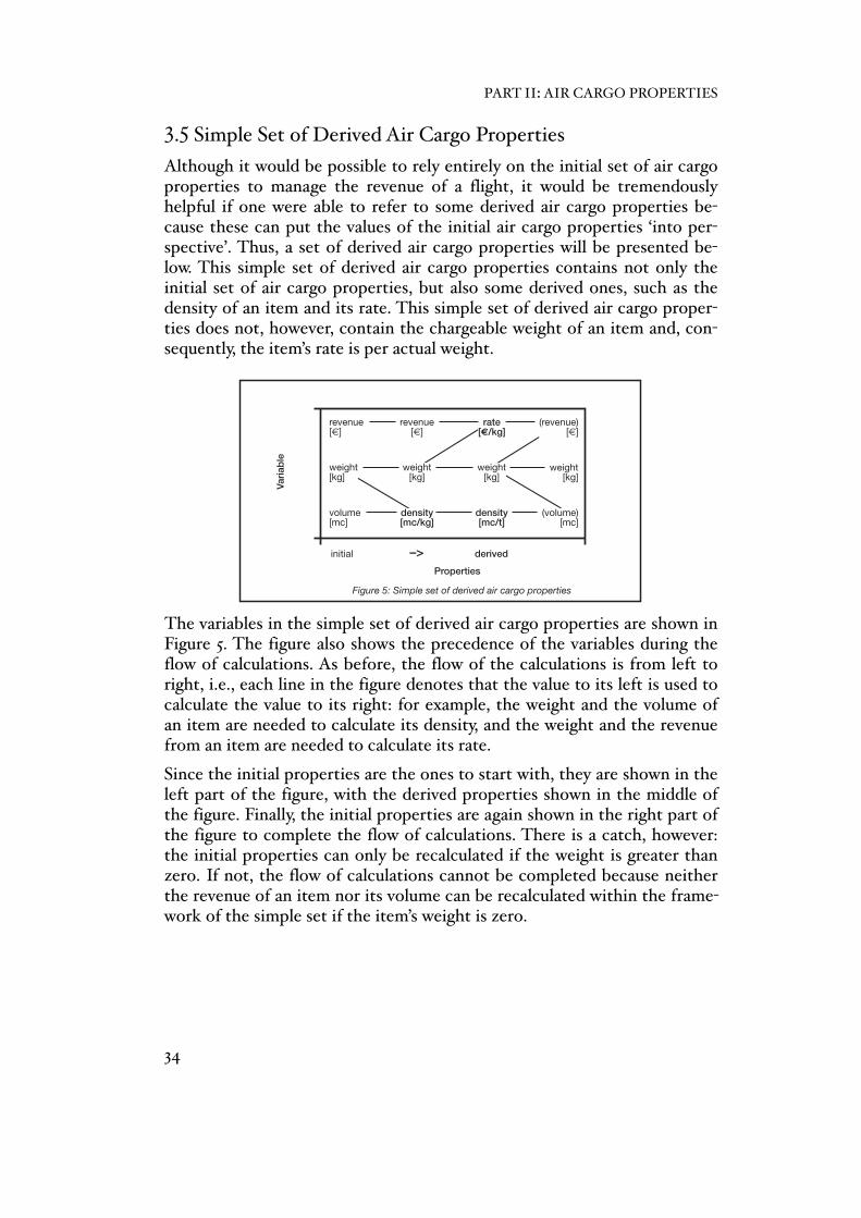
3.5 Simple Set of Derived Air Cargo Properties

Although it would be possible to rely entirely on the initial set of air cargo properties to manage the revenue of a flight, it would be tremendously helpful if one were able to refer to some derived air cargo properties be-cause these can put the values of the initial air cargo properties ‘into per-spective’. Thus, a set of derived air cargo properties will be presented be-low. This simple set of derived air cargo properties contains not only the initial set of air cargo properties, but also some derived ones, such as the density of an item and its rate. This simple set of derived air cargo proper-ties does not, however, contain the chargeable weight of an item and, con-sequently, the item’s rate is per actual weight.

The variables in the simple set of derived air cargo properties are shown in Figure 5. The figure also shows the precedence of the variables during the flow of calculations. As before, the flow of the calculations is from left to right, i.e., each line in the figure denotes that the value to its left is used to calculate the value to its right: for example, the weight and the volume of an item are needed to calculate its density, and the weight and the revenue from an item are needed to calculate its rate.

Since the initial properties are the ones to start with, they are shown in the left part of the figure, with the derived properties shown in the middle of the figure. Finally, the initial properties are again shown in the right part of the figure to complete the flow of calculations. There is a catch, however: the initial properties can only be recalculated if the weight is greater than zero. If not, the flow of calculations cannot be completed because neither the revenue of an item nor its volume can be recalculated within the frame-work of the simple set if the item’s weight is zero.

mpsmwps mvps

XX

Varia

ble

–> derivedinitial

Figure 5: Simple set of derived air cargo properties

Properties

Chargeable weight density scaling for high density freight

0 1/12 1/6 1/4 1/3 5/12 1/2

Unified Density [–]C

harg

eabl

e W

eigh

t [ch

kg]

1.0

0.8

0.6

0.4

0.2

0

6

CD

0 1 32 54

void

void

Density [mc/t]

BCAB

CD'

BC'

AB'

volume c

onsumptio

n

weight consumption

No chargeable weight density scaling for low density freight

Unified Density [–]

Cha

rgea

ble

Wei

ght [

chkg

]

1.0

0.8

0.6

0.4

0.2

0

6

void

void

Density [mc/t]

7 98 1110 12

FGEFDE

FG'EF'

DE'

0.5 0.75

weight consumption

volume consumption

8/117/106/95/84/7

Figure 28: Legend of some of the primal parameters and variables

0 10 20 30 40 6050

4.00

3.50

3.00

2.50

2.00

0.50

1.50

1.00

0.00


Rat

e [€

/chk

g]

qis

ris fwcl

sisxis

fr

Figure 31: Legend of some of the dual parameters and variables

0 10 20 30 40 6050

4.00

3.50

3.00

2.50

2.00

0.50

1.50

1.00

0.00


Rat

e an

d C

ost [

€/c

hkg]

qis

ris

pis

uis

mwpl

fr

bwclbwcl

mps

2 4 96 18

Rat

e [€

/chk

g]

Figure 36: Marginal and full segment prices, and the dual modes

Density [mc/t]

9r

8r

7r

6r

5r

4r

3r

2r

1 0 = r

0 !

mwps

mvps

fps

fvps

fwps definitely profitable(dual mode 1)

profitable(dual mode 2)

not profitable(dual mode 3)

10 = cw

2cw

3cw

4cw

5cw

6cw

cwharg

eabl

e W

eigh

t [ch

t]

bcsbwcs

mps

Rat

e [€

/chk

g]

9r

8r

7r

6r

5r

4r

3r

2r

1 0 = r

mwps

mvps

fp

a

a

s

fvps

fwps definitelyprofitable

profitable

not profitable

feasible

rActual Booking

Request

Actual BookingRequest

q10 = cw

2cw

3cw

4cw

5cw

6cw

cwharg

eabl

e W

eigh

t [ch

t]

bcsbwcs

Rat

e [€

/chk

g]

9r

8r

7r

6r

5r

4r

3r

2r

1 0 = r

fps

fvps


profitable

feasible

fcsfvcs

fwcs

definitely feasible



fvcsfwcs fcs

s

a

ar

q

density[mc/t]

(revenue)[€]

revenue[€]

revenue[€]

rate[€/kg]

weight[kg]

(volume)[mc]

weight[kg]

weight[kg]

volume[mc]

density[mc/kg]

weight[kg]


34

This set of derived air cargo properties is not only remarkably simple (hence its name), the variables and definitions in the simple set are often used in commercial Cargo Revenue Management Systems. Moreover, the variables and definitions in the simple set of derived air cargo properties are often used in the scientific literature on Cargo Revenue Management (see, for example, Kasilingam 1996, Couzy 2004, Klabjan and Sandhu 2005, Pak 2005, Bartodziej and Derigs 2004, as well as Derigs et al. 2006). Never-theless, the simple set of derived air cargo properties has some disad-vantages which are not easily overcome.

These disadvantages are:

❖ The derived air cargo properties in the simple set cannot replace the initial air cargo properties for items that have zero weight. In other words, the weight, the rate per weight, and the density of an item are no substitute for the item’s weight, volume, and revenue.

❖ The simple set of derived air cargo properties cannot easily be adapted to deal with items that have zero weight. If, for example, the simple set was instead based on the volume as the main dimen-sion (rather than the weight), the simple set would then not be able to deal with items that have a zero volume.

❖ The simple set of derived air cargo properties does not explicitly contain the chargeable weight; the simple set is focused on the physical aspects of transportation.

❖ Within the simple set of derived air cargo properties, the weight and the volume are treated as two separate dimensions and cannot easily be compared.

❖ Since the simple set of derived air cargo properties does not contain the chargeable weight, the set cannot take advantage of the charge-able weight’s advanced features (i.e., of being a universal economic term, of being able to reduce the number of different quantity units, and of having favourable dimensional scaling).

❖ The rates in the simple set of derived air cargo properties are different from the market rates (which are per chargeable weight). Moreover, the rates in the simple set of derived air cargo properties are rates per input factor (i.e., per weight or per volume) and not rates per output product (i.e., per chargeable weight).

To overcome these disadvantages, an extended set of derived air cargo properties is required and this will be presented next.


35

3.6 Extended Set of Derived Air Cargo Properties

The extended set contains the initial set of air cargo properties plus the following derived air cargo properties: the chargeable weight, the weight and volume coefficients, the rate per chargeable weight, and the density.

The initial and derived air cargo properties of the extended set are shown in Figure 6. Also shown in the figure are the precedence of the properties and the flow of calculations. The main difference between the extended and the simple sets of derived air cargo properties is that the extended set is centred on the chargeable weight rather than the actual weight. Conse-quently, all weights and volumes are expressed in terms of their chargeable weight, and the rate is also per chargeable weight.

The formulas to recalculate the initial air cargo properties from the derived air cargo properties of the extended set are presented below. These formu-las are called “reversed formulas”.

Reversed Formulas of the Extended Set:W = w × cw × wcV = (v × cw × vc)/chtcR = r × cw

All the formulas needed to calculate the values of a particular column from the values in the preceding column have now been presented. Other formu-las representing the multitude of relationships between the various items in Figure 6 have not been given here but can easily be determined.

It is important to note that most of the presented formulas are valid for individual items only. The chargeable weight of multiple bookings, for example, cannot be calculated using the bookings’ combined weight and volume, but only by calculating the chargeable weights of the bookings one by one.

estsla

estslaamaxsl

critical

qslqsl

dsl

v sl

wsl

weight co-efficient with

stowage loss*

Den

sity

Mix

of T

wo

Item

s [%

]

Uni

fied

Den

sity

Lab

els

0 1 32 54

7.2 6 void

void6

12 9! 36 18

200

166

133

100

Density [mc/t]

Density [mc/t]

Density mix and extremeness of density

–1 –.833 –.5–.66 –.166–.33 0 void

Extremeness of Density [–]

!"

Figure 41: Propagation of stowage loss

Varia

ble

density withstowage

loss*

revenue

weight

revenue

effectivedemand*

volume withstowageloss*

volume withstowage

loss*

weight

revenue

volume co-efficient with

stowage loss*

effectivedemand*

effectiverate*

rasl

–>

The standard density and its components


Varia

ble

wc[kg/chkg]

tc[kg/t]

chtc[chkg/cht]

tc[kg/t]

tc[kg/t]

tc[kg/t]

vc/wc[mc!chkg/cht/kg]

ds[mc/t]

vc[mc/cht]

ds[mc/t]

chtc[chkg/cht]

chtc[chkg/cht]

chtc[chkg/cht]

–> derivedinitial

Properties (*including Stowage Loss)


–> derivedinitial

Propagation of stowage loss

Varia

ble

revenue[euro]

revenue[euro]

chargeableweight*[chkg]

volume*[mc]

volume*[mc]

weight[kg]

revenue[euro]

weightcoefficient*[chkg/chkg]


rate*[euro/chkg]

volumecoefficient*[chkg/chkg]

density*[mc/t]

weight[kg]

–> derivedinitial

Figure 6: Extended set of derived air cargo properties

Properties

Varia

ble

revenue[€]

revenue[€]


volume[mc]

volume[mc]

weight[kg]

revenue[€]

weightcoefficient

[chkg/chkg]


rate[€/chkg]

volumecoefficient

[chkg/chkg]

density[mc/t]

weight[kg]

0 1 32 54 7.2

scaled density

6 129 !3618

0 1 32 54 7

range split: “0 – 6” and “6 – 12”

6 98 121110

w0 w1 w3w2 w5w4 v5

weight and volume prefix: “w” and “v”

6 v3v4 v0v1v2

0 1 32 54 v5

volume prefix: “v”

6 v3v4 v0v1v2

0 1 32 54 – 5

volume prefix: “–”

6 – 3– 4 – 0– 1– 2

Density Labels [unitless] and Density [mc/t]

Figure 18: Various labels for unified density

Figure 44: Stowage loss bar

optimise …

Volume Stowage Loss [mc]

7sl6sl5sl4sl3sl2sl

Figure 47: Stowage loss ranges for an actual booking request

rejectconfirm

fp mpbc


7sl6sl5sl4sl3sl2sl

optimise rejectconfirm

fp mpbc

Sto

wag

e Lo

ss R

ange

s

sdc

0 = 1sl0 = 1sl

sdc

aa

a

a

a

amaxsl estsla


36

The proposed set of derived air cargo properties can be further extended by adding costs. A cost extension makes sense because, after all, the suc-cessful management of revenue is comparable to the successful manage-ment of costs. The confirmation of a booking request, for example, usually not only means that a certain revenue will be earned, but also that some other booking requests cannot be confirmed which, in turn, means that the extra revenue from the accepted booking request comes at a cost (i.e., there is a displacement cost). Furthermore, if these costs are to be com-pared with a revenue rate, both the rate and the costs need to be expressed in the same quantity unit. In other words, it is advantageous to add the costs to the extended set of derived air cargo properties and to calculate unit costs using the same quantity unit as that for the rates. Within the ex-tended set of derived air cargo properties, this common quantity unit is euro per chargeable kilogram.

To display the proposed cost extension within the usual framework, the costs and the unit costs have been incorporated in Figure 7 below, which shows the precedence of the variables and the flow of calculations within the extended set of air cargo properties, adapted to include costs.

You will observe that Figure 7 is similar to Figure 6, the only difference be-ing that rate and revenue in Figure 6 have been replaced by costs and unit costs in Figure 7. The costs are considered to be an initial air cargo property and the unit costs are considered as a derived air cargo property.

The definition of unit costs within the extended set of derived air cargo properties is as follows: if the chargeable weight of an item is greater than zero, the unit costs are calculated as the cost of the item divided by its chargeable weight; if the chargeable weight is zero, the unit costs are not defined.



1 5.623.161.77 31.17.10 56. 562.316.177.100 1000

… pi-i2 pi-i1 p0 …

keine Skalierung

21 positiond

0 1 32 54 7


6 98 121110



0 1 32 54 7.2

(5; 11)

(5; 13)

(6; 11)

(6; 13)

6 129 !3618

Ska

lieru

ngen

0 0.2 0.60.4 0.8 1.251 2.51.66 !5

0 1.2 3.62.4 64.8

6.25 12.5 25

7.5 1510 !30

0 1 32 54 !

0 0.833 2.51.66 4.1663.33 65 107.5 !3015

8.33



0 1.09 3.272.18 5.454.36 6.6

(1 ; 10 )

(5; 10)

(5; 12)

(6; 10)

(6; 12)

118.25 !3316.5

Ska

lieru

ngen

0 1.125 2.251.5 !4.5

0 4

5.625 11.25 22.5

6.75 13.59 !27

0 !

0 0.90 2.721.81 4.543.63 5.5 9.166.875 !27.513.75

7.5

1.33 2.66 5.33

1.11 2.22 3.33 4.44

0.880.660.440.22


Bes

chre

ibun

g



3)

2)1)

Sta

ndar

d–Vo

lum

enge

wic

ht1)

Anz

ahl v

on P

ositi

onen

2)S

tand

ard–

Volu

men

gew

icht

1)

Anz

ahl v

on P

ositi

onen

2)

(1 ; 11 )2)1)


Set an Positionen

1 … …32


2)1)

circ

a A

ngab

en3)

Sta

ndar

d–Vo

lum

enge

wic

ht1)

Anz

ahl v

on P

ositi

onen

2)

pi-i2 pi-i1 p


Bes

chre

ibun

g un

d S

kalie

rung


10

position

Set an Positionen



!0 pi-i1dpi-i2d3d2d

1 … …32

ds

1/23ud2ud

0 1/12 1/41/6 5/121/3 7/12


1/2 3/42/3 111/125/6

0 1 32 54 7.2


6 129 !3618


positionud


positiond

Sta

ndar

d–Vo

lum

enge

wic

ht1)

Anz

ahl v

on P

ositi

onen

2)

2)1)

XVII





d[mc /t ]

Chargeable

[chkg ]Weight cw

[kg ] [mc ]

0.0060.601.000.60101

0.0061.001.001.0061

0.0041.000.661.0041

0.0021.000.331.00210.0011.000.161.00110.0001.000.001.0001

0.0051.000.831.0051

0.0060.661.000.6691

0.0031.000.501.0031

0.0060.851.000.85710.0060.751.000.7581

………………0.0060.001.000.00!1

"

"

"

"

"

"

"

"

–>



Varia

ble



volume[mc]

standarddensity

[mc/t]


weight[kg]

weight[kg]

–>



Varia

ble


volume[mc]

volume[mc]

standarddensity

[mc/t]

weight[kg]

weight[kg]

–> derivedinitial


Properties

Varia

ble

cost[€]

cost[€]


volume[mc]

volume[mc]

weight[kg]

cost[€]

weightcoefficient

[chkg/chkg]


unit cost[€/chkg]

volumecoefficient

[chkg/chkg]

density[mc/t]

weight[kg]

density[mc/t]


unifieddensity

[unitless]

scaleddensity[mc/t]

or

volume[mc]

density[mc/t]




37

The following list contains the advantages of using the extended set of de-rived air cargo properties (including unit costs):

❖ The extended set of derived air cargo properties can deal with zero weight and zero volume.

❖ The extended set of derived air cargo properties includes two values which are basic in the air cargo industry, i.e., the chargeable weight and the rate per chargeable weight.

❖ The use of the chargeable weight, its density, and the rate per charge-able weight may reveal some of the airfreight’s more interesting, market-related economic characteristics, while the use of the weight, the volume, and the revenue is more suited to the physical aspectsand the accounting needs of transportation.

❖ The weight and volume coefficients in the extended set of derived air cargo properties reflect the inherent similarity of the (specific) weight and volume consumption. If, for example, the weight and volume coefficients of an item are 0.5 and 1 respectively, the volume consumption of the item is twice as great as its weight consumption.

❖ By using the chargeable weight of the extended set, the weight and the volume of an item can be directly compared. The 20% difference between 10,000 chargeable kilograms of pure weight and 12,000 chargeable kilograms of pure volume is, for example, easier to spot than the same percentage difference between a weight of 10,000 kilograms and a volume of 72 cubic metres.

❖ By calculating and using the unit costs in the extended set of derived air cargo properties, a check of cost similarities becomes notably easier. This is especially true if some of the costs are based on weight or volume alone. A fuel surcharge of 0.10 euro per kilogram, for example, can hardly be compared with volume displacement costs of 200.– euro per cubic metre. If, however, the costs are calculated as unit cost per chargeable kilogram, a comparison becomes much easier. The units costs of the fuel surcharge, to continue with the given example, would be 0.10 euro per chargeable kilogram, while the unit costs of the volume displacement would be 1.20 euro per chargeable kilogram. It is now easy to see that the volume displacement costs are twelve times higher than the fuel surcharge.

❖ The use of the variables in the extended set not only allows a side-by-side comparison of weight and volume unit costs (or, more accurately, a side-by-side comparison of the unit costs of any given density), but also a side-by-side comparison of the unit costs and the rates.


38

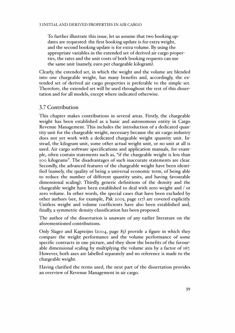
To further illustrate this issue, let us assume that two booking up-dates are requested: the first booking update is for extra weight, and the second booking update is for extra volume. By using the appropriate variables in the extended set of derived air cargo proper-ties, the rates and the unit costs of both booking requests can use the same unit (namely, euro per chargeable kilogram).

Clearly, the extended set, in which the weight and the volume are blended into one chargeable weight, has many benefits and, accordingly, the ex-tended set of derived air cargo properties is preferable to the simple set. Therefore, the extended set will be used throughout the rest of this disser-tation and for all models, except where indicated otherwise.

3.7 Contribution

This chapter makes contributions in several areas. Firstly, the chargeable weight has been established as a basic and autonomous entity in Cargo Revenue Management. This includes the introduction of a dedicated quan-tity unit for the chargeable weight, necessary because the air cargo industry does not yet work with a dedicated chargeable weight quantity unit. In-stead, the kilogram unit, some other actual weight unit, or no unit at all is used. Air cargo software specifications and application manuals, for exam-ple, often contain statements such as, “if the chargeable weight is less than 100 kilograms”. The disadvantages of such inaccurate statements are clear. Secondly, the advanced features of the chargeable weight have been identi-fied (namely, the quality of being a universal economic term, of being able to reduce the number of different quantity units, and having favourable dimensional scaling). Thirdly, generic definitions of the density and the chargeable weight have been established to deal with zero weight and / or zero volume. In other words, the special cases that have been excluded by other authors (see, for example, Pak 2005, page 117) are covered explicitly. Unitless weight and volume coefficients have also been established and, finally, a symmetric density classification has been proposed.

The author of the dissertation is unaware of any earlier literature on the aforementioned contributions.

Only Slager and Kapteijns (2004, page 85) provide a figure in which they compare the weight performance and the volume performance of some specific contracts in one picture, and they show the benefits of the favour-able dimensional scaling by multiplying the volume axis by a factor of 167. However, both axes are labelled separately and no reference is made to the chargeable weight.

Having clarified the terms used, the next part of the dissertation provides an overview of Revenue Management in air cargo.


39

PART III: OVERVIEW OF REVENUE MANAGEMENT IN AIR CARGO

4 Basics of a Cargo Revenue Management System

An air cargo carrier usually has numerous flights under its control and, more often than not, the freight has to ‘connect’ to make its way from its origin to its destination. The same is true for passengers, but in contrast to the wishes and requirements of passengers, the route or the departure time of freight is not generally of concern as long as it reaches its final destina-tion by a certain time.

The booking request control of connecting freight is also referred to as Origins & Destinations control (for a discussion of O&D control see Hol-loway 2003, pages 532ff., 549f., and 551ff.).

It is logical that the Revenue Management System of an air cargo carrier should take into account all scheduled flights simultaneously, i.e., the Cargo RMS should confirm or reject each booking request so that the overall revenue of the air cargo carrier’s network of flights is maximised. This, however, is a daunting task and, therefore, as a first step, the focus of this dissertation is on developing a theory to maximise the revenue from a sin-gle flight (note that the definition of a flight includes interim stops).

A single flight has three entities: the leg(s), the segment(s), and the flight itself. Attached to these entities are the weight and volume capacities, the customer demands, and the flight revenues.

A detailed definition of what exactly is considered to be a flight, a segment, and a leg will be given in the first section of this chapter. In the second sec-tion, the terms ‘flight revenue’, ‘segment demand’, and ‘leg capacity’ will be defined and, in the third section, the bookings, the booking requests, and the booking process will be discussed. Rates, densities, and routes are the issues discussed in the fourth section, and the chapter ends with a state-ment of its contributions to the subject.

4.1 Flight, Segment, and Leg

Among a carrier’s various flights, a particular flight can be identified by its flight ID. The flight ID is a combination of the carrier code, the flight num-ber, and the departure date. The string “AV 123 01.02.2005”, for example, is the flight ID of a domestic flight from Cali (CLO) to Cartagena de Indias (CTG). This flight is operated by Avianca (AV), departs from Cali on the given date at 08:00 o’clock in the morning, and has a stopover in Santafé de Bogotá (BOG). The flight has two legs (CLO–BOG and BOG–CTG) and three segments (CLO–BOG, BOG–CTG, and CLO–CTG).

In this dissertation, there is no separate index for the flight identification attribute since it is assumed throughout the dissertation that all symbols relate to the same flight ID (where applicable). It should be noted that the

41

leg departure dates and the segment departure dates are not necessarily the same as the flight departure date: only the first leg and the first segment of a flight automatically share the date and time of the flight’s departure.

The following relationships apply between the legs of a flight, its segments, and the flight itself: every flight has one or more legs, and every segment covers one or more consecutive legs. Typically, each possible combination of consecutive flight legs is a flight segment. The relationships are depicted in Figure 8.

The upper part of the figure shows the flight level of AV 123, the central part (between the dotted lines) shows the segment level of the flight, and the lower part of the figure shows the flight at the leg level.

To identify a flight’s legs and segments, their indices are introduced below.

Flight Leg and Flight Segment Indices:s+ flight segment indexl+ flight leg index

The value ranges of the leg and segment indices of a flight both start with the number 1 and, in practice, a flight rarely exceed 5 legs and 15 segments.

The flight segment coefficient indicates whether a flight leg is part of a specific flight segment, and is introduced and defined below.

Flight Segment Incidence Coefficient:als+ {0, 1} [unitless]+ incidence coefficient of flight leg l+ + + + on flight segment s

Flight Segment Incidence Coefficient as a Function of Traversed Legs:if+ flight leg l is part of flight segment s+ + then als = 1elseif+ flight leg l is not part of flight segment s++ then als = 0

As has already been stated, the flight segment incidence coefficient is unit-less and takes either the value “0” or “1”.

0 6/5 3 6 12 !30

2

1

0

Density [mc/1000 kg]

weight

volume

Soll eine Buchungsanfrage bestätigt werden, oder nicht?

Primal Mode

Dua

l Mod

e

4 65

yes no

no

nono

yes

yes

IV

0,00

0 2 4 96 !18

4,00

3,50

3,00

2,50

2,00

0,50

1,50

1,00

0,00


Bid

Pric

e [e

uro/

chkg

]

Bid–Preise für einen gewichts- und volumenkritischen Flug

State

Rea

lisat

ion

No knowledge of first period demand realisation

Init

Init 1 2

State

Rea

lisat

ion

Knowledge of first period demand realisation

1 2

Bildunterschrift

Volume [mc]

0 1 2 3 4 5 6 7.2 9 !12 18 36

2

1

0


weight

volume

0 1/5 1/2 1 2 5

2

1

0


weight volume

optimize

1

2

3 notpossible

Weight [kg]

Bildunterschrift

Volume [mc]Weight [kg]

Bildunterschrift


Bildunterschrift


0.007

0.006

0.005

0.004

0.001

0.003

0.002

0.000

!

0.007

0.006

0.005

0.004

0.001

0.003

0.002

0.000

0.007

0.006

0.005

0.004

0.001

0.003

0.002

0.000

Cartagenade Indias

CTG

Cartagenade Indias

CTG

Cartagenade Indias

CTG

Cartagenade Indias

CTG

CaliCLO

CaliCLO

CaliCLO

CaliCLO

Santaféde Bogotá

BOG

Santaféde Bogotá

BOG

Figure 8: Flight with two legs and three segments

leg leg

Cities and their Airport Three Letter Codes

flight

segment segment

Leg,

Seg

men

t and

Flig

ht L

evel

segment

!"#$


42

4.2 Flight Revenue, Segment Demand, and Leg Capacity

In this dissertation it is assumed that the revenue is earned at the flight level, that the demand originates at the segment level, and that the weight and volume capacities are given at the leg level.

The Flight Revenue

The flight revenue initially shares many features of the revenue that was described in Section 3.1 as an initial air cargo property.

The flight revenue is usually a variable (as opposed to a constant or a para-meter), the unit of the flight revenue is [€], and its value range is restricted in practice to nonnegative and finite values. Having such a restriction on value range for flight revenue, however, can be inconvenient if the variable is used as an objective variable within a mathematical program (since objec-tive variables of mathematical programs are usually free variables), and for this reason it is assumed that the value of the flight revenue ranges from minus infinity to plus infinity. This revised value range of the flight revenue is used in the definition below.

Flight Revenue (Revised Value Range):fr + [– ∞, ∞] [€]+ + flight revenue

However, this change to the value range is largely academic since the flight revenues that are computed in this dissertation are always nonnegative (and limited). There is an exception, however: when a flight revenue is used as an objective value in a mathematical program that has no feasible solution, then the flight revenue is considered to have a value of minus infinity (in the case of a maximisation problem) or plus infinity (in the case of a mini-misation problem) to indicate that the mathematical program is infeasible (see, for example, Eiselt et al. 1987, pages 564f., for a discussion on the rela-tionship between an infeasible mathematical program and its assumed ob-jective value).

The Segment Demand

The term ‘demand’ is not only used to denote the chargeable weight of a single booking request but also for the combined chargeable weights of fu-ture bookings which will be requested for a particular flight segment during the remaining booking period (hence the name ‘segment demand’). The segment demand is a demand-to-come.

Segment Demand:qs+ [0, ∞) [chkg]+ + demand-to-come for flight segment s

The segment demand is usually a parameter (as opposed to a variable or a constant) and is expressed in chargeable kilograms.

4 BASICS OF A CARGO REVENUE MANAGEMENT SYSTEM

43

Since the segment demand is a demand-to-come, it cannot be negative, nor can the segment demand of a departed flight segment be greater than zero.

The Leg Capacity

Initially, a leg’s weight and volume capacities share many features with the initial air cargo properties weight and volume, as defined in Section 3.1. The difference is that the weight and volume capacities are stated in terms of their chargeable weight, whereas the initial air cargo properties weight and volume are stated in kilograms and cubic metres. More specifically, the weight capacity is stated in terms of a chargeable weight that has a zero density, and the volume capacity is stated in terms of a chargeable weight that has an infinite density. The weight capacity of a first flight leg may be, for example, 1,000 chargeable kilograms (the equivalent of 1,000 kilo-grams), while the volume capacity of that flight leg may be 2,000 charge-able kilograms (the equivalent of 12 cubic metres).

The formulas for converting weight and volume to chargeable weight are given below; they are similar to the reversed formulas of the extended set presented earlier in Section 6 of Chapter 3.

Chargeable Weight of ‘Pure’ Weight and ‘Pure’ Volume:W [chkg] = W [kg]/wcV [chkg] = (V [mc]/vc) chtc

With regard to the calculation of a leg’s weight and volume capacities, there is a major difference between freighters and the belly capacity of passenger flights because belly capacity is consistently calculated as the capacity remaining after the weight of the (expected) passengers and the (anticipated) baggage weight and volume have been subtracted.

The bookable leg weight and volume capacities are introduced below.

Bookable Leg Weight and Volume Capacities:bwcl+ [0, ∞) [chkg]+ + bookable weight capacity of flight leg lbvcl+ [0, ∞) [chkg]+ + bookable volume capacity of flight leg l

The bookable capacities are defined as the leg weight and volume capa-cities available to accommodate any bookings that might be requested between the present time and the leg departure time. The value ranges of the bookable capacities are restricted to nonnegative numbers, although in practice they could be negative.

The reasons why the leg weight and volume capacities can be negative are as follows:

❖ The payload is reduced during the booking period due to more-than-expected passenger bookings (on passenger flights).

❖ Products with guaranteed capacity access (e.g., express cargo) have been heavily sold.


44

❖ Overbooking limits have been reduced.

❖ A (large) booking request has been manually confirmed (‘forced’), even though there was insufficient capacity.

A booking period can also start with negative weight and volume capaci-ties, for example, when a lot of weight and volume has been blocked for special reasons.

The problem with negative capacities is that they make many mathemat-ical optimisation models that could be used in Air Cargo Revenue Manage-ment infeasible. An example of a model which will become infeasible if one or more of the leg weight and volume capacities are negative is the primal model that can be used to calculate the flight revenue (this model will be presented in the first section of Chapter 7). The reason that this model be-comes infeasible is that no positive demand forecast can fill negative ca-pacities.

In spite of being mathematically infeasible, a flight with negative weight and volume capacities can still earn a positive revenue because, more often than not, only one leg capacity will be negative and the other leg capacities are zero or positive. In practice, therefore, a negative leg capacity would result in closing all segments that involve that particular leg, but a negative leg capacity would not result in closing the flight, and other segments which use only legs that have a positive remaining capacity are still open for sale. Shortly before departure, the flight will be ‘cleaned up’ by rebook-ing freight or by using a larger plane, and so, in the end, the revenue of the flight can still be positive.

The Modified Leg Capacity

Since there is no reason to rule out such a positive flight revenue, when using a mathematical program, the adverse effects of a negative capacity on the feasibility of these models must be avoided. One way of achieving this is to simply replace any negative leg weight and volume capacity with a zero leg weight and volume capacity, as suggested below.

Modified Leg Weight and Volume Capacities:bwcl = max {0, bwcl}bvcl = max {0, bvcl}

The above modification to the leg capacities does not result in a model that offers the possibility of rebooking the freight or changing the flight equipment. There is also little chance that the ‘modified’ flight revenue will be equal to the ‘real world’ revenue (which would be achieved after the nec-essary rebooking or equipment change have been undertaken). However, it is likely that the ‘modified’ flight revenue will be, in many cases, reasonably close to the ‘real world’ revenue, especially if one consider the fact that negative capacities during the booking period are often only temporary. In


45

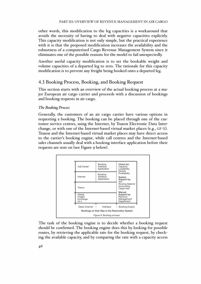
other words, this modification to the leg capacities is a workaround that avoids the necessity of having to deal with negative capacities explicitly. This capacity modification is not only simple, but the practical experience with it is that the proposed modification increases the availability and the robustness of a computerised Cargo Revenue Management System since it eliminates one of the possible reasons for the model to fail unexpectedly.

Another useful capacity modification is to set the bookable weight and volume capacities of a departed leg to zero. The rationale for this capacity modification is to prevent any freight being booked onto a departed leg.

4.3 Booking Process, Booking, and Booking Request

This section starts with an overview of the actual booking process at a ma-jor European air cargo carrier and proceeds with a discussion of bookings and booking requests in air cargo.

The Booking Process

Generally, the customers of an air cargo carrier have various options in requesting a booking. The booking can be placed through one of the cus-tomer service centres, using the Internet, by Traxon Electronic Data Inter-change, or with one of the Internet-based virtual market places (e.g., GF-X). Traxon and the Internet-based virtual market places may have direct access to the carrier’s booking engine, while call centres and the Internet-based sales channels usually deal with a booking interface application before their requests are sent on (see Figure 9 below).

The task of the booking engine is to decide whether a booking request should be confirmed. The booking engine does this by looking for possible routes, by retrieving the applicable rate for the booking request, by check-ing the available capacity, and by comparing the rate with a capacity access

Overbooking and decrementing

30 days

Overbooked Capacity

150%

100%

50%

DepartureLAT

4000

3500

3000

2500

2000

500

1500

1000

0

Time Prior to Departure

Wei

ght [

kg]

VII

Cancellations

Physical Capacity

No Shows

CancellationsNo Shows

xxxxxxxxxxxxxxxxx

xxxxxx

xxxxxx

Check for:CapacityLoadabilityDensityProfitability

SystemSupport by:MosaikRouting SelectorCRASEagle

ManualSupport by:F/MR Queue

The (future) booking process

Bookings on their Way to Mosaik

easyBooking

eBooking

CSCCall Center

Internet

Traxon

GlobalFreightExchangeGF-X

Bildunterschrift

0 5 15Booking EngineInterfaceSales Channel 10 2520 35 45 5530 40 6050

400

350

300

250

200

50

150

100

0

Achsenbezeichnung [Einheit]

Ach

senb

ezei

chnu

ng [E

inhe

it]

»»

Eagle supports the booking engine in making the decision

Information Flow

Booking, ifRequest isConfirmed

Bid Price

Confirmationor Rejection

Eagle calculates the bid price

Optimising …

Eagle

CRAS easyBooking

Eagle

Booking Engine

Mosaik

A booking is requested via easyBooking

Information Flow

easyBooking

Eagle

Booking Requestand Rate

Rate Booking Request

Booking Engine

MosaikCapacity

Remaining

CRAS

Transforming units of production into units of sales

View

Weight[kg]

Volume[mc]

Price per Char-geable Weightof Density Infinity[euro/chkg]

Price per Char-geable Weightof Density Zero[euro/chkg]

ChargeableWeight ofDensity Infinity[chkg]

ChargeableWeight ofDensity Zero[chkg]

ChargeableWeight[kg]

Density[mc/1000 kg]

Rate perChargeableWeight[euro/chkg]

ProductionTransformedSales

Price perVolume[euro/mc]

Price perWeight[euro/kg]

Check for:CapacityLoadabilityDensityProfitability

SystemSupport by:RESRouting SelectorAccountingCargo RMS

ManualSupport by:RevenueManagementDepartment

Figure 9: Booking process

Bookings on their Way to the Reservation System

BookingInterfaceApplication

BookingInterfaceApplication

Call Center

Internet

Traxon

GlobalFreightExchangeGF-X

Booking EngineInterfaceSales Channel »»


46

price, if applicable. If, for whatever reason, the booking engine can neither confirm nor reject a booking request, it will be sent to a queue to be exam-ined individually. Finally, a confirmed booking request is sent to the air cargo carrier’s reservation system (also known as ‘RES’).

Usually, a cargo booking can be requested from as early as 30 days to as late as two hours before the flight departs (such short times apply only to small pieces of express cargo). However, if the flight has several segments, a cargo booking can be requested and confirmed even after the flight has departed its home base. This is because the booking period is defined relative to the departure time of the requested segment of the respective flight. In other words, a booking can be made as long as the flight has not departed the lo-cal airport and there is sufficient handling time.

The Booking (Request)

Next follows a discussion on bookings and booking requests in the air cargo industry. The discussion starts by defining booking requests for a par-ticular flight ID, using booking request index b.

Booking Request Index:b+ booking request index

The set of all booking requests for this flight ID is then B.

Set of Booking Requests:B+ + + + set of all booking requests

Since the set B includes all booking requests, it makes sense to introduce several subsets of B. The subset Bp consists only of past booking requests, Bf consists only of future booking requests, and Ba is the subset that con-tains only the current booking request.

Subsets of Booking Requests:Bp+ + + + set containing all past booking requestsBf+ + + + set of all future booking requestsBa+ + + + set containing the actual booking request + + + + under consideration

Clearly, Bp ∪ Ba ∪ Bf equals B; and Bp ∩ Ba, Ba ∩ Bf, and Bp ∩ Bf are empty. The actual booking request is identified by its index value b being equal to a, and the set of past booking requests includes all bookings which were requested before the actual booking was requested, while the set of future booking requests includes all bookings which will be requested after the actual booking has been requested. It is assumed that there is, at most, only one actual booking request—the one that has to be confirmed or re-jected ‘right now’. In this way, the members of Bp and Bf are defined relative to the actual booking request. To indicate its special role it is denoted, from now on, not as the booking request for which the index value is equal to a (as in Wb = a), but simply as booking request a (as in Wa).


47

Finally, a subset of subset Bp is introduced: Bpc, the set of all past bookings that have been confirmed.

Set of Past Bookings:Bpc+ + + + set containing all past confirmed bookings

The initial properties of an air cargo booking request are its weight, its vol-ume, and its revenue; and its derived properties are its demand, its rate, and its density. The demand, the rate, and the density are seen as the three dimensions of a booking (request) since they represent its most important characteristics.

The symbols and the value ranges of a booking request’s initial and derived air cargo properties are listed below.

Weight, Volume and Revenue of a Booking Request:Wb+ [0, ∞) [kg]+ + weight of booking request bVb+ [0, ∞) [mc]+ + volume of booking request bRb+ (0, ∞) [€]+ + revenue of booking request b

Derived Air Cargo Properties of a Booking Request:rb+ (0, ∞) [€/chkg]+ rate of booking request bwb+ [0, 1] [chkg/chkg]+ weight coefficient of booking request bvb+ [0, 1] [chkg/chkg]+ volume coefficient of booking request bdb+ [0, ∞] [mc/t]+ + density of booking request bqb+ (0, ∞) [chkg]+ + demand (quantity) of booking request b

Most of the above value ranges turn out in reality to be more limited if the practicalities of the actual air cargo business are considered. The majority of booking requests, for example, have a chargeable weight of less than 10,000 chargeable kilograms, a density between 3 and 12 cubic metres per tonne, a rate between 1.– and 2.– euro per chargeable kilogram, and a rout-ing over only one or two legs. These limits are, however, liable to change and, therefore, they have not been used to restrict the above value ranges.

Booking requests that have a zero revenue or a zero rate are considered as outliers, as are booking requests that have a zero demand (i.e., a zero chargeable weight).

It is also important to note that the demand, density, and rate values which are valid at the time a booking is requested are, strictly speaking, not the ones which are important: the true weight and volume consumptions of a booking request are usually not known exactly until departure—and the booked values are very likely to change until then. Hence, the relevant point in time to refer to with regard to the weight and volume of a booking request is the departure time of the requested segment. A similar reasoning applies to the rate of a booking request: the relevant moment to refer to is the payment’s due date. However, even though this differentiation might seem odd at first, it is not, since there are many reasons why the weight and the volume of a booking request can change, and even more reasons why the rate of a booking request can (and will) change. Among the reasons


48

for changed weights and volumes are booking updates, rebookings, and cancellations (it is also possible that a booking simply does not show up). Overall, the most prominent reason for changed rates is that the rates that were initially offered were only used to get preferred capacity access—so-mething which happens quite often in the industry. However, these issues are not relevant for the purposes of this dissertation and, therefore, all cal-culations will be based on the values as booked (i.e., as declared).

The coefficient used to show the existence of a flight leg on the requested segment is called the booking request incidence coefficient.

Booking Request Incidence Coefficient:alb+ {0, 1} [unitless]+ incidence coefficient of flight leg l+ + + + on the flight segment of booking request b

Booking Request Incidence Coefficient as a Function of Traversed Legs:if+ flight leg l is part of the flight segment of booking request b then alb = 1elseif+ flight leg l is not part of the flight segment of booking request b then alb = 0

The formulas for obtaining the demand of a booking request, its density, the booking request’s weight and volume coefficients, as well as its rate, are given below. They are stated here only briefly since they resemble formulas explained earlier.

The first formula calculates the demand of a booking request.

Demand of a Booking Request as a Function of its Weight and Volume:if+ Wb/wc ≥ (Vb/vc) chtc + then qb = Wb/wcelseif+ Wb/wc < (Vb/vc) chtc + then qb = (Vb/vc) chtc

As defined here, the demand of a requested booking is equal to its charge-able weight. Note that demand in air cargo is usually lumpy and booking requests can rarely be confirmed for part of a load. Moreover, booking re-quests in air cargo can be quite large: 20% of the bookings may very well use 80% of the flight’s capacity. The passenger (or hotel guest) equivalent of lumpy demand in air cargo is a group booking by several passengers (hotel guests). Hence, the literature on Passenger Revenue Management and Hotel Revenue Management also considers lumpiness in demand (see, for example, Yuen 2002).

The next formulas are for calculating the density, the weight and volume coefficients, and the rate of a booking request.

Density of a Booking Request as a Function of its Weight and Volume:if+ Wb = 0 and Vb = 0+ + then db is indeterminateelseif+ Wb > 0 and Vb ≥ 0+ + then db = (Vb/Wb) tcelseif+ Wb = 0 and Vb > 0+ + then db = ∞

Weight and Volume Coefficients of a Booking Request as a Function of its Density:if+ db is indeterminate+ + then wb and vb are indeterminateelseif+ 0 ≤ db ≤ sdc + + + then wb = 1 and vb = db/sdcelseif+ sdc < db < ∞+ + + then wb = sdc/db and vb = 1elseif+ db = ∞++ + + then wb = 0 and vb = 1


49

Rate of a Booking Request as a Function of its Revenue and Chargeable Weight:if+ qb = 0+ + + + then rb is indeterminateelseif+ qb > 0+ + + + then rb = Rb/qb

The rate has a prominent role in the air cargo business even though it is not considered as an initial air cargo property. The prominence of the rate is because the negotiations between air cargo carriers and their customers are usually not about the revenue of the cargo but about its rate (the rate per chargeable weight, that is). Thus, in one sense, the rate is only a derived air cargo property but, then again, the rate is as real as the weight or the volume.

It is important to note that there is a strong relationship between the size of a shipment and its rate, with small shipments tending to have higher rates than large shipments. This is due to minimum revenues, chargeable weight breakpoints, and the negotiation power of customers who request large bookings (for further discussion on the subject see, for example, Doganis 2002, pages 317 and 324f.). The minimum revenue of a booking request could be, for example, 50.– euro, while the chargeable weight break-points are usually at 100 chargeable kilograms and 500 chargeable kilo-grams.

Since the rates typically decrease immediately that a chargeable weight breakpoint has been reached, it may make sense for a customer to declare a higher nominal chargeable weight to get a lower rate because, by doing so, the customer may be able to reduce the amount he has to pay to the carrier in exchange for transporting the freight. Essentially, the idea behind this so-called ‘bumping’ is to flatten the cost function near the chargeable weight breakpoints (see the dotted lines in Figure 10).

It should be noted that since the lower rate is related to the higher weight, the lower rate is as nominal as the higher weight. In order to get the real rate of a booking request (i.e., the rate r, which is related to the booking request’s real chargeable weight), the nominal chargeable weight has to be multiplied by the nominal rate, and the result of that multiplication has to be divided by the real chargeable weight (i.e., the chargeable weight q, which is related to the booking request’s real weight and volume).

In Figure 10, it is assumed that the minimum revenue R for a particular segment is 50.– euro per booking request, the rate r100 for bookings up to 100 chargeable kilograms is 1.– euro per chargeable kilogram, the rate r500 for bookings up to 500 chargeable kilograms is 0.73 euro per chargeable kilogram, and the rate r500+ for bookings greater than 500 chargeable kilo-grams is 0.66 euro per chargeable kilogram.


50

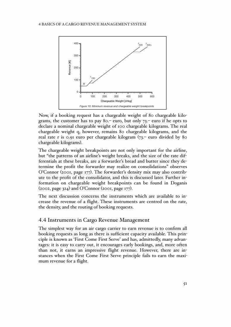
Now, if a booking request has a chargeable weight of 80 chargeable kilo-grams, the customer has to pay 80.– euro, but only 73.– euro if he opts to declare a nominal chargeable weight of 100 chargeable kilograms. The real chargeable weight q, however, remains 80 chargeable kilograms, and the real rate r is 0.91 euro per chargeable kilogram (73.– euro divided by 80 chargeable kilograms).

The chargeable weight breakpoints are not only important for the airline, but “the patterns of an airline’s weight breaks, and the size of the rate dif-ferentials at these breaks, are a forwarder’s bread and butter since they de-termine the profit the forwarder may realize on consolidations” observes O’Connor (2001, page 177). The forwarder’s density mix may also contrib-ute to the profit of the consolidator, and this is discussed later. Further in-formation on chargeable weight breakpoints can be found in Doganis (2002, page 324) and O’Connor (2001, page 177).

The next discussion concerns the instruments which are available to in-crease the revenue of a flight. These instruments are centred on the rate, the density, and the routing of booking requests.

4.4 Instruments in Cargo Revenue Management

The simplest way for an air cargo carrier to earn revenue is to confirm all booking requests as long as there is sufficient capacity available. This prin-ciple is known as ‘First Come First Serve’ and has, admittedly, many advan-tages: it is easy to carry out, it encourages early bookings, and, more often than not, it earns an impressive flight revenue. However, there are in-stances when the First Come First Serve principle fails to earn the maxi-mum revenue for a flight.

u > 0ij x > 0ij

XVIII


Com

plem

enta

ry S

lack

ness

Con

ditio

n


u = 0ij

s > 0ij p = 0ij

u = 0ijs = 0ij

p > 0ij

x = 0ijp = 0ij

p = 0iju =ij

x = 0ij

ijijp = 0 ! x

ijijp = x = 0

u = 0 ! sijij


u " 0 < sijij

x =ij Dij

0 ! x !ij Dij


0 10 20 30 40 6050

4.00

3.50

3.00

2.50

2.00

0.50

1.50

1.00

0.00


Rat

e [e

uro/

chkg

]

Wk

demandforecast


BCxBCx


0 10 20 30 40 6050

4.00

3.50

3.00

2.50

2.00

0.50

1.50

1.00

0.00


Rat

e [e

uro/

chkg

]

Wk

demandforecast


BCoptr

minBCr

BCr

WkBCD– BCw

optmax

0 1 2 43 65

4

3

2

1

0

Weight [t]

Volu

me

[mc]


# m

c/t

4 m

c/t

2 m

c/t

1.33

mc/

t

1 mc/

t

0.8 mc/t

0 mc/t

0.66 mc/t

1)

stan

dard

den

sity

(das

hed)

: 6 c

ubic

met

res

per t

onne

1)


0 20 40 60 80 120100

4.00

3.50

3.00

2.50

2.00

0.50

1.50

1.00

0.00


Rat

e [€

/chk

g]

–> derivedinitial


Properties

Varia

ble

revenue[€]

revenue[€]


volume[mc]

weight[kg]

revenue[€]

weightcoefficient

[chkg/chkg]


rate[€/chkg]

volumecoefficient

[chkg/chkg]


weight[kg]

0 100 200 400300 500

400

300

200

100

0


Rev

enue

[€]

600


100r

500+r

500r

R

Density [mc/t]

Rat

e [€

/chk

g]


s

disl dis

u

risu

risl

domaindemandqis

i

disdomaindensity

risdomain

ratex

x

x

x

x

x x

xx

x

x

density[mc/t]

volume[mc]

m

np

u

NW(s, x) NE(s, u)

SW(p, x) SE(p, u)

D =ij 0x =ij

m

ijijp " 0 = xn


nn

s>=0

s=0

u>=0


51

To understand why the First Come First Serve principle may lead to sub-optimal decisions, it is helpful to review the instruments which are avail-able to an air cargo carrier to increase the revenue of a single flight.

The instruments are:

❖ Confirm only booking requests that have favourable rates.

❖ Prefer booking requests that have suitable densities.

❖ Mix booking requests that have high and low densities.

❖ Opt for booking requests that involve short routes.

❖ Combine booking requests that have diverse routings.

These instruments need certain preconditions to be fulfilled in order to be effective. First of all, the rates of at least some of the booking requests have to be different because it would not otherwise be possible to make a dis-tinction between favourable and unfavourable rates. Secondly, the densities of at least some of the booking requests have to be different; otherwise, it would not be possible to make a distinction between suitable densities and unsuitable densities. Moreover, a prerequisite for the third instrument is that there must be at least one booking request that falls into the high-density category and at least one booking request that falls into the low-density category in order to be able to mix the densities effectively. The fourth prerequisite is that in order to be able to opt for short routes, it is necessary that not all booking requests have the same number of legs. Fi-nally, the prerequisite for a combination of diverse routings to be effective is that the routes of at least some of the booking requests are indeed dif-ferent; otherwise it would be difficult to balance flight leg utilisation. Of course, the routing-related instruments can only be used on itineraries where the routing matters, i.e., on flights that have multiple legs and mul-tiple segments. Below is a more detailed discussion of the instruments.

The Favourable Rate of a Booking Request

Confirming favourable rates is the art of rejecting booking requests that have less favourable rates if these booking requests are not needed to fill a plane. The skill here is to decide how many low-rate booking requests should be rejected: rejecting too many low-rate booking requests may result in an underloaded flight, while the rejection of too few low-rate booking requests may result in the need to reject some high-rate booking requests later in the booking period. The use of this instrument in air cargo has also been described by O’Connor (2001, page 194).

Note that the order in which the high- and low-rate bookings are requested is quite important because if all the high-rate bookings are requested first (i.e., before any low-rate bookings are requested), the problem of managing the flight revenue is less difficult than if the low-rate bookings are re-


52

quested ahead of the high-rate bookings. However, even if the incoming order of the booking requests is strictly ‘high before low’, there is no guar-antee that a First Come First Serve type sequential confirmation will achieve the maximum possible flight revenue because the rates per charge-able weight do not necessarily reflect the revenue contributions of the booking requests. This is because the revenue contribution of a booking request not only depends on its rate, but also on its density and its route.

The Suitable Density of a Booking Request

The preferential confirmation of booking requests that have suitable den-sities may give an air cargo carrier the opportunity to increase the charge-able weight of a flight beyond its most limiting weight or volume capacity. The most limiting weight or volume capacity is also known as the short capacity, and booking requests that have a suitable density are either high-density or low-density, depending on whether the flight is short on volume or short on weight. (To find out whether a flight is short on weight or short on volume, the weight capacity has to be converted from kilograms to chargeable kilograms that have a zero density, and the volume capacity has to be converted from cubic metres to chargeable kilograms that have an infinite density because, only then, can both capacities be directly com-pared; see the formulas for the chargeable weight of pure weight and vol-ume in Section 2 of Chapter 4). The most suitable densities, however, are all at least as high as the density of the remaining flight capacity (if it is high-density), or at least as low (if it is low-density).

On a more general level, the use of this instrument has been described by O’Connor (2001, page 187): “Sales policy of an airline may also be directed at the cube-out problem of aircraft. Its sales personnel may be directed to refrain from soliciting low-density traffic, but to promote high-density traf-fic aggressively. The object should be to try to get the best mix for the types of aircraft in the airline’s fleet.” He also describes the common prac-tice in air cargo of offering a high-density bonus to avoid an early cube-out (see O’Connor 2001, page 192).

The Mixing of High- and Low-Density Booking Requests

Mixing high- and low-density booking requests is an instrument that can increase the chargeable weight of a flight even further. The working prin-ciple of this instrument is to ‘assemble’ bookings that have a suitable density by fitting together several high- and low-density booking requests (preferably booking requests that have extreme densities) and to use the re-captured weight and volume to confirm additional booking requests—and thus more chargeable weight—than would otherwise be possible.


53

The example below not only demonstrates the advantages of confirming booking requests that have a suitable density, it also shows the advantages of mixing high- and low-density booking requests:

A flight is assumed to have a remaining weight capacity of 10,000 charge-able kilograms (the equivalent of 10,000 kilograms) and a remaining vol-ume capacity of 20,000 chargeable kilograms (the equivalent of 120 cubic metres). Clearly, there is less weight available than there is volume avail-able, and the density of the remaining flight capacity is 12 cubic metres per tonne.

The weight capacity is the most limiting since it limits the flight’s charge-able weight to 10,000 chargeable kilograms. That is, no more than 10,000 chargeable kilograms can be confirmed if it is assumed that the requested bookings have a standard density. However, if the booking requests had a density of 12 cubic metres per tonne, up to 20,000 chargeable kilograms could be confirmed (10,000 kilograms and 120 cubic metres, to be spe-cific).

Alternatively, if two large booking requests have densities of 4 cubic metres per tonne and 20 cubic metres per tonne respectively, the chargeable weight of the flight can be up to 21,666 chargeable kilograms by ‘assem-bling’ a suitable booking of 10,000 kilograms and 120 cubic metres out of these high- and low-density booking requests. In fact, the confirmation of the high-density booking request (that with a density of 4 cubic metres per tonne) and the confirmation of the low-density booking request (that with a density of 20 cubic metres per tonne) will result in 21,666 chargeable kilograms, with the first booking request contributing 5,000 kilograms, 20 cubic metres, and 5,000 chargeable kilograms, and the second booking re-quest contributing 5,000 kilograms, 100 cubic metres, and 16,666 charge-able kilograms.

The preferential confirmation of booking requests with suitable densities would double the flight’s chargeable weight in the given example from 10,000 chargeable kilograms to 20,000 chargeable kilograms; the mix of high- and low-density bookings would increase the flight’s chargeable weight to 21,666 chargeable kilograms. The maximum chargeable weight of the flight is 30,000 chargeable kilograms but this has not been achieved in the given example since the tripling of the flight’s chargeable weight would have required the confirmation of extremely high- and low-density booking requests, and these were not available.

As has been shown in the example above, the objective of preferring suit-able densities as well as the objective of mixing high and low densities is to ‘circumvent’ the capacity limitations of a flight in order to accommodate a greater amount of chargeable weight. This is possible because high-density booking requests consume comparatively little volume per chargeable kilo-


54

gram and low-density booking requests consume comparatively little weight per chargeable kilogram. However, the opportunity to confirm booking requests that have suitable densities and of mixing high and low densities clearly depend on whether bookings with these densities are in-deed requested. One option is for demand to be stimulated by offering an incentive (a so-called density bonus) to encourage high- and low-density booking requests.

Incidentally, a similar process of mixing extreme densities is known among forwarders as consolidation. The difference between consolidation and the air cargo carriers use of density mix is that the forwarders do not try to cir-cumvent some fixed capacities but merely a soft constraint. The soft con-straint that forwarders face is that they have to pay the air cargo carriers for the weight and the volume they bring, and bringing weight and volume in densities other than the standard density increases the chargeable weight and hence the transport costs of the freight. Forwarders are effec-tively rewarded for consolidating high- and low-density shipments into one booking request that has a density close to the standard density. A short note about consolidation in the air cargo industry from the forwarder’s per-spective can be found in Logistics Management (2002). See also the third section of this chapter and the section on the role of the freight forwarders in Doganis (2002, pages 315-318).

The Short Route of a Booking Request

The next instrument which may help to increase the chargeable weight of a flight is to opt for booking requests involving as few legs as possible (pref-erably only one) because the preferential confirmation of such booking requests may permit the confirmation of other booking requests on other legs, thus increasing the chargeable weight of the flight.

The Mixing of Booking Requests with Various Routings

Combining booking requests with various routings is another instrument that can increase the chargeable weight of a flight. The working principle of this instrument is to grant capacity access only to booking requests (preferably single-leg booking requests) that will contribute to an evenly distributed flight-leg capacity utilisation, thus avoiding bottleneck situa-tions which may lead to an underutilisation on other legs.

The Use of the Instruments

It is apparent that the above described instruments cannot be applied in-dependently since if a booking request is confirmed on a particular flight, all of the booking request’s features will be confirmed, including the rate of the booking request, its density, and its route (and no matter that some of the booking request’s features might be unwanted).


55

Thus, the situation is that a booking request will frequently have some beneficial features and some negative features, and the former may, or may not, outweigh the latter.

It is now becoming clear why the First Come First Serve principle may fail to optimise revenue: the First Come First Serve principle does not deter-mine capacity access using any of the booking request features and it is very unlikely that booking requests with beneficial features will be re-quested first (not forgetting that the benefits of a booking request’s fea-tures depend upon the features of the other booking requests). In fact, the First Come First Serve principle will only achieve the maximum revenue if the flight has enough capacity to confirm all the requested bookings. If the flight does not have enough capacity to confirm all the requested bookings, a Cargo Revenue Management System can in principle be used to maximise revenue.

An effective Cargo RMS estimates the current bookable capacity, forecasts future booking requests, plans ahead by optimising the flight’s rate-, den-sity-, and route-mix, and confirms (or rejects) actual booking requests in order to maximise the revenue of the flight. In other words, a Cargo Reve-nue Management System performs a leg capacity forecast, a segment de-mand forecast, a flight revenue optimisation, and booking request control.

4.5 Contribution

The contribution of this chapter is mainly in two areas: firstly, the air cargo carrier’s supply has been expressed in the same units as the customers’ de-mand (i.e., in chargeable kilograms), and secondly, Cargo Revenue Manage-ment instruments to increase the revenue of a single flight have been iden-tified. More specifically, the preferential confirmation of suitable densities, the use of high and low densities, the mixing of high and low densities into a suitable density, and the fact that all of these instruments interrelate have, to the best knowledge of the author, not previously been described of useable level in the literature, i.e., these instruments have been mentioned only very briefly in the literature, and neither the techniques nor their pre-requisites have been discussed explicitly.

Doganis (2002), for example, although he seems to be aware of suitable densities and the density mix, is somewhat vague and not fully correct in his formulations when he writes on page 311 that “an airline must try to achieve an average density in its freight carrying which makes maximum use of both the volumetric capacity and the weight payload of its aircraft” and on page 324 that “by mixing shipments of different weight and density in a container, one can reduce the average cargo rate paid to the airline” (which aims at the density mix from the point of view of the forwarder, but ignores the carrier).


56

Further, O’Connor (2001), although he mentions the rate mix, the cube-out problem, and the high-density incentive discount, does not elaborate on these ideas.

The paper by Cakanyildirim and Moussawi (2005) is a little more specific on the prerequisites of an optimal density mix by implying on pages 9f. that if the density of all booking requests is either below or above the standard density, the combined chargeable weight of the booking requests is equal to the chargeable weight of their combined weight and volume. Since, how-ever, the paper is mainly about overbooking, no method is suggested for intentionally using the density mix or density bonuses to increase the reve-nue of a flight.

Finally, Holloway (2003, page 594) recommends that “high-volume cargo which ‘wastes’ payload capacity (as well as high-density cargo which ‘wastes’ volume capacity) should, ideally, be priced to offer attractive yields in com-pensation”, a recommendation that obstructs use of the density mix—at least if Holloway means to impose rate-per-chargeable-weight penalties on booking requests that have an extreme density.

To further develop the basics of an effective Cargo Revenue Management System, nonlinear density scaling has to be introduced. Hence, the next part of the dissertation is about the various densities in air cargo.


57

PART IV: NONLINEAR DENSITY SCALING

5 Various Densities in Air Cargo

The purpose of this chapter is to discuss various volume-to-weight ratios and to identify which of them can capture the similarities of items having a weight, a volume, and a chargeable weight. Incidentally, this is a task which resembles the construction of a geographical map or the construction of a homogeneous colour space, as it involves, it will turn out, a change of the dimensions in which the object is represented.

Linear density will be discussed in the first section, followed by unified density and scaled density in the second section. The contribution of this chapter will be summarised in the third section.

5.1 Linear Density

The linear density (or the regular density, as it is also known) is the density ‘as is’. The linear density is thus the density that has been defined in the previous chapters.

The Density ‘as is’

The use of the density ‘as is’ will result in a similarity that considers that two items that have densities of, say, 1 and 2 respectively are as similar as any other two items that have densities that differ by one unit. It is ques-tionable, however, whether this is a similarity which would be supported by economic reasoning, or whether it is only a similarity of numbers. To inves-tigate further, an analysis of the weight and volume consumption of one chargeable kilogram with various densities is considered.

Figure 11 shows the specific weight and volume consumptions of one chargeable kilogram that has a density between zero (i.e., 0 cubic metres per tonne) and the standard density (i.e., 6 cubic metres per tonne).

60 1 32 54

Density [mc/t]

volume c

onsumptio

n

weight consumption

Clustering with chargeable weight density scaling

0 1 2 3 4 5 6 7.2 9 !12 18 36

1.0

0.8

0.6

0.4

0.2

0

Density [mc/t]

Cha

rgea

ble

Wei

ght [

chkg

]

0 1 2 3 4 5 6 7 8 129 10 11

1.0

0.8

0.6

0.4

0.2

0

Density [mc/t]

Clustering without chargeable weight density scaling

Cha

rgea

ble

Wei

ght [

chkg

]

JI

I

H

Hv

v

w

w

vww wv v

K

L

L

Figure 11: Specific weight and volume consumption of high-density freight

Cha

rgea

ble

Wei

ght [

chkg

]

Figure 12: Specific weight and volume consumption of low-density freight

Cha

rgea

ble

Wei

ght [

chkg

]


Figure 13: Unified density of low density-freight

Cha

rgea

ble

Wei

ght [

chkg

]

1.0

0.8

0.6

0.4

0.2

0

void

void

Density [mc/t]

1/2 7/12 2/3 3/4 5/6 111/12

FGEFDEFG'

EF'

DE'

K

K

J

L

I

I

H

H

Bildunterschrift

0 1 2 3 4 5 6 7.2 9 !12 18 36

1

0

Density [mc/t]

weight

volume0.006

0.005

0.004

0.001

0.003

0.002

0.000


Bildunterschrift

0 1 2 3 4 5 6 7 8 129 10 11

1

0

Density [mc/t]

weight

volume0.006

0.005

0.004

0.001

0.003

0.002

0.000


LK

v

v

w

w

vww wv v

6 7.2 9 !12 18 36

weight consumption

volume consumption

XVI


Figure 14: Unified density and scaled density

Cha

rgea

ble

Wei

ght [

chkg

]

1.0

0.8

0.6

0.4

0.2

0

1/2 7/12 2/3 3/4 5/6 111/12

6 7.2 9 !12 18 36

weight consumption

volume consumption

0 1/12 1/6 1/4 1/3 5/12

1.0

0.8

0.6

0.4

0.2

0

6void

Density [mc/t]

7 98 1110 12

FGEFDE

FG'EF'

DE' weight consumption

volume consumption1.0

0.8

0.6

0.4

0.2

0

6

CD

0 1 32 54 void

Density [mc/t]

BCAB

CD'

BC'

AB'

volume c

onsumptio

n

weight consumption

59

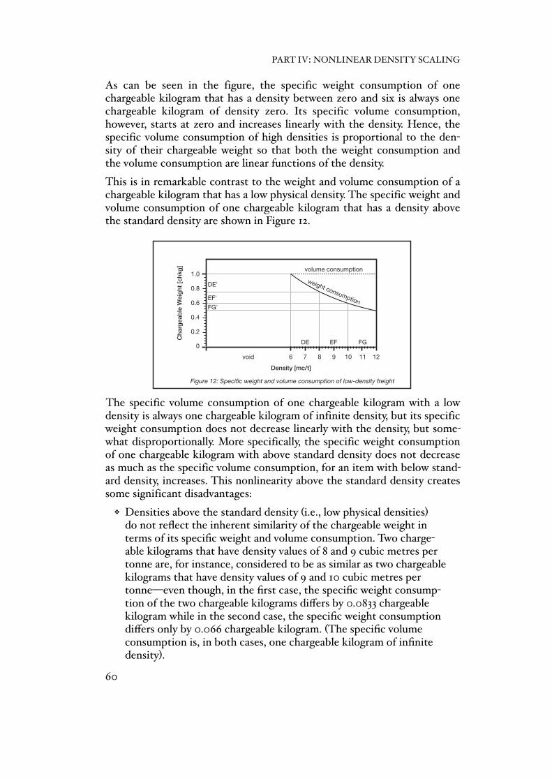
As can be seen in the figure, the specific weight consumption of one chargeable kilogram that has a density between zero and six is always one chargeable kilogram of density zero. Its specific volume consumption, however, starts at zero and increases linearly with the density. Hence, the specific volume consumption of high densities is proportional to the den-sity of their chargeable weight so that both the weight consumption and the volume consumption are linear functions of the density.

This is in remarkable contrast to the weight and volume consumption of a chargeable kilogram that has a low physical density. The specific weight and volume consumption of one chargeable kilogram that has a density above the standard density are shown in Figure 12.

The specific volume consumption of one chargeable kilogram with a low density is always one chargeable kilogram of infinite density, but its specific weight consumption does not decrease linearly with the density, but some-what disproportionally. More specifically, the specific weight consumption of one chargeable kilogram with above standard density does not decrease as much as the specific volume consumption, for an item with below stand-ard density, increases. This nonlinearity above the standard density creates some significant disadvantages:

❖ Densities above the standard density (i.e., low physical densities) do not reflect the inherent similarity of the chargeable weight in terms of its specific weight and volume consumption. Two charge-able kilograms that have density values of 8 and 9 cubic metres per tonne are, for instance, considered to be as similar as two chargeable kilograms that have density values of 9 and 10 cubic metres per tonne—even though, in the first case, the specific weight consump-tion of the two chargeable kilograms differs by 0.0833 chargeable kilogram while in the second case, the specific weight consumption differs only by 0.066 chargeable kilogram. (The specific volume consumption is, in both cases, one chargeable kilogram of infinite density).

60 1 32 54

Density [mc/t]

volume c

onsumptio

n

weight consumption


0 1 2 3 4 5 6 7.2 9 !12 18 36

1.0

0.8

0.6

0.4

0.2

0

Density [mc/t]

Cha

rgea

ble

Wei

ght [

chkg

]

0 1 2 3 4 5 6 7 8 129 10 11

1.0

0.8

0.6

0.4

0.2

0

Density [mc/t]


Cha

rgea

ble

Wei

ght [

chkg

]

JI

I

H

Hv

v

w

w

vww wv v

K

L

L


Cha

rgea

ble

Wei

ght [

chkg

]


Cha

rgea

ble

Wei

ght [

chkg

]



Cha

rgea

ble

Wei

ght [

chkg

]

1.0

0.8

0.6

0.4

0.2

0

void

void

Density [mc/t]

1/2 7/12 2/3 3/4 5/6 111/12

FGEFDEFG'

EF'

DE'

K

K

J

L

I

I

H

H

Bildunterschrift

0 1 2 3 4 5 6 7.2 9 !12 18 36

1

0

Density [mc/t]

weight

volume0.006

0.005

0.004

0.001

0.003

0.002

0.000


Bildunterschrift

0 1 2 3 4 5 6 7 8 129 10 11

1

0

Density [mc/t]

weight

volume0.006

0.005

0.004

0.001

0.003

0.002

0.000


LK

v

v

w

w

vww wv v

6 7.2 9 !12 18 36

weight consumption

volume consumption

XVI



Cha

rgea

ble

Wei

ght [

chkg

]

1.0

0.8

0.6

0.4

0.2

0

1/2 7/12 2/3 3/4 5/6 111/12

6 7.2 9 !12 18 36

weight consumption

volume consumption

0 1/12 1/6 1/4 1/3 5/12

1.0

0.8

0.6

0.4

0.2

0

6void

Density [mc/t]

7 98 1110 12

FGEFDE

FG'EF'

DE' weight consumption

volume consumption1.0

0.8

0.6

0.4

0.2

0

6

CD

0 1 32 54 void

Density [mc/t]

BCAB

CD'

BC'

AB'

volume c

onsumptio

n

weight consumption


60

❖ The similarity of two densities cannot be determined if one of the density values is infinity. How (dis)similar is, for example, a density of 10 cubic metres per tonne to an infinite density?

❖ Infinite densities—as well as density values which are close to infini-ty—are difficult to display on a linear scale, even though items that have an infinite density are not uncommon in the air cargo industry (e.g., volume booking updates).

❖ The left part of a linear density axis (i.e., the part between density zero and the standard density) is much shorter than the right part of the density axis (i.e., the part between the standard density and density infinity). Although this lack of proportion is not a problem per se, it hinders an unbiased view of the density distribution.

The main consequence of the said nonlinearity is that a variation in the specific volume consumption of a chargeable kilogram that has a high den-sity will lead to a smaller change in the density than a comparable variation in the specific weight consumption of a chargeable kilogram that has a low density. In other words, similar changes in the specific weight and volume consumptions are not treated similarly—even though there is no reason to treat high and low densities (or weight and volume, for that matter) differ-ently.

5.2 Unified Density and Scaled Density

The disadvantages of using linear density, as discussed above, can be avoided by using the so-called unified density. Unified density is a new concept in air cargo transportation. It can be used not only to manage revenue but also for many other purposes as diverse as the creation of density-dependent pricing schemes, the specification of two-dimensional overbooking algorithms, the definition of outlying densities, the creation of symmetrical booking classes, and the generation of realistic booking request data for revenue simulations.

The Unified Density and the Scaled Density

The unified density allows the specific weight and volume consumption of a chargeable kilogram to be expressed as a linear function of its density, it helps to identify the degree of similarity between different densities, whether they are high or low, and it creates symmetry and balance between the weight and the volume by giving them equal weighting (hence the name “unified density”).

5 VARIOUS DENSITIES IN AIR CARGO

61

The unified density is considered as a derived air cargo property and is specified using the declaration below.

Unified Density:ud+ [0, 1] [unitless]+ unified density

The symbol for the unified density is ud, and its value ranges from pure weight, with a unified density of zero, to pure volume, with a unified den-sity of one. The definition of the unified density is given below.

Unified Density as a Function of Weight and Volume:if+ W = 0 and V = 0+ + then ud is indeterminateelseif+ W > 0 and (V/W) tc ≤ sdc+ then ud = (V/W) (tc/2sdc)elseif+ V > 0 and (V/W) tc > sdc+ then ud = 1 – (W/V) (sdc/2tc)

Regular and unified densities can be converted into each other with the help of the following two formulas.

Unified Density as a Function of Density:if+ d is indeterminate+ + then ud is indeterminateelseif+ 0 ≤ d ≤ sdc+ + + then ud = d/(2sdc)elseif+ sdc < d < ∞+ + + then ud = 1 – (sdc/2d)elseif+ d = ∞+ + + + then ud = 1

Density as a Function of Unified Density:if+ ud is indeterminate ++ then d is indeterminateelseif+ 0 ≤ ud ≤ 0.5+ + + then d = 2ud sdcelseif+ 0.5 < ud < 1+ + + then d = sdc/(2 – 2ud)elseif+ ud = 1+ + + + then d = ∞

To avoid a nonlinear decrease in the specific weight consumption above the standard density, the unified density re-scales the low-density part of the linear density axis as shown in Figure 13 below.

The figure shows the specific weight consumption of one chargeable kilo-gram as a function of its unified density

60 1 32 54

Density [mc/t]

volume c

onsumptio

n

weight consumption


0 1 2 3 4 5 6 7.2 9 !12 18 36

1.0

0.8

0.6

0.4

0.2

0

Density [mc/t]

Cha

rgea

ble

Wei

ght [

chkg

]

0 1 2 3 4 5 6 7 8 129 10 11

1.0

0.8

0.6

0.4

0.2

0

Density [mc/t]


Cha

rgea

ble

Wei

ght [

chkg

]

JI

I

H

Hv

v

w

w

vww wv v

K

L

L


Cha

rgea

ble

Wei

ght [

chkg

]

1.0

0.8

0.6

0.4

0.2

0

6

CD

0 1 32 54 void

Density [mc/t]


Cha

rgea

ble

Wei

ght [

chkg

]

1.0

0.8

0.6

0.4

0.2

0

6void

Density [mc/t]

7 98 1110 12

FGEFDE

FG'EF'

DE'

BCAB

CD'

BC'

AB'



Cha

rgea

ble

Wei

ght [

chkg

]

1.0

0.8

0.6

0.4

0.2

0

void

void

Density [mc/t]

1/2 7/12 2/3 3/4 5/6 111/12

FGEFDEFG'

EF'

DE'

K

K

J

L

I

I

H

H

Bildunterschrift

0 1 2 3 4 5 6 7.2 9 !12 18 36

1

0

Density [mc/t]

weight

volume0.006

0.005

0.004

0.001

0.003

0.002

0.000


Bildunterschrift

0 1 2 3 4 5 6 7 8 129 10 11

1

0

Density [mc/t]

weight

volume0.006

0.005

0.004

0.001

0.003

0.002

0.000


LK

v

v

w

w

vww wv v

6 7.2 9 !12 18 36

volume c

onsumptio

n

weight consumption

weight consumption

volume consumption

weight consumption

volume consumption

XVI



Cha

rgea

ble

Wei

ght [

chkg

]

1.0

0.8

0.6

0.4

0.2

0

1/2 7/12 2/3 3/4 5/6 111/12

6 7.2 9 !12 18 36

weight consumption

volume consumption

0 1/12 1/6 1/4 1/3 5/12


62

After the rescaling, a move along the unified density axis does, now, lead to a linear change in the specific weight consumption of a chargeable kilo-gram with a low density. The vertical distances DE’, EF’, and FG’, for example, are all the same length (as can be seen in Figure 13), which is in contrast to Figure 12, in which a linear density increase above the standard density leads to a nonlinear change in the specific weight consumption of a chargeable kilogram.

Figure 13 also shows the so-called scaled density. Scaled density is essen-tially the unified density displayed as a regular density. The advantage of displaying scaled density rather than unified density is that the scaled den-sity is closer to the industry’s established nomenclature (i.e., the density, since unified density is unknown in the industry), while, at the same time, the density figures are arranged as if they were unified.

The specific weight and volume consumptions of a chargeable kilogram across the full density range are displayed in Figure 14. The figure also shows the unified density and the scaled density (dubbed ‘Density’) over the full density range.

The specific weight and volume consumptions are also known as the weight and volume coefficients of the chargeable weight. The formulas for the weight and volume coefficients of a chargeable kilogram, as a function of its unified density, are given below.

Weight and Volume Coefficients as a Function of Unified Density:if+ ud is indeterminate ++ then w and v are indeterminateelseif+ 0 ≤ ud ≤ 0.5+ + + then w = 1 and v = 2udelseif+ 0.5 < ud ≤ 1+ + + then w = 2 – 2ud and v = 1

As can easily be recognised, the specific weight and volume consumptions of a chargeable kilogram are linear if expressed as a function of its unified density.

60 1 32 54

Density [mc/t]

volume c

onsumptio

n

weight consumption


0 1 2 3 4 5 6 7.2 9 !12 18 36

1.0

0.8

0.6

0.4

0.2

0

Density [mc/t]

Cha

rgea

ble

Wei

ght [

chkg

]

0 1 2 3 4 5 6 7 8 129 10 11

1.0

0.8

0.6

0.4

0.2

0

Density [mc/t]


Cha

rgea

ble

Wei

ght [

chkg

]

JI

I

H

Hv

v

w

w

vww wv v

K

L

L


Cha

rgea

ble

Wei

ght [

chkg

]

1.0

0.8

0.6

0.4

0.2

0

6

CD

0 1 32 54 void

Density [mc/t]


Cha

rgea

ble

Wei

ght [

chkg

]

1.0

0.8

0.6

0.4

0.2

0

6void

Density [mc/t]

7 98 1110 12

FGEFDE

FG'EF'

DE'

BCAB

CD'

BC'

AB'


Figure 13: Unified density of low density-freightC

harg

eabl

e W

eigh

t [ch

kg]

1.0

0.8

0.6

0.4

0.2

0

void

void

Density [mc/t]

1/2 7/12 2/3 3/4 5/6 111/12

FGEFDEFG'

EF'

DE'

K

K

J

L

I

I

H

H

Bildunterschrift

0 1 2 3 4 5 6 7.2 9 !12 18 36

1

0

Density [mc/t]

weight

volume0.006

0.005

0.004

0.001

0.003

0.002

0.000


Bildunterschrift

0 1 2 3 4 5 6 7 8 129 10 11

1

0

Density [mc/t]

weight

volume0.006

0.005

0.004

0.001

0.003

0.002

0.000


LK

v

v

w

w

vww wv v

6 7.2 9 !12 18 36

volume c

onsumptio

n

weight consumption

weight consumption

volume consumption

weight consumption

volume consumption

XVI



Cha

rgea

ble

Wei

ght [

chkg

]

1.0

0.8

0.6

0.4

0.2

0

1/2 7/12 2/3 3/4 5/6 111/12

6 7.2 9 !12 18 36

weight consumption

volume consumption

0 1/12 1/6 1/4 1/3 5/12


63

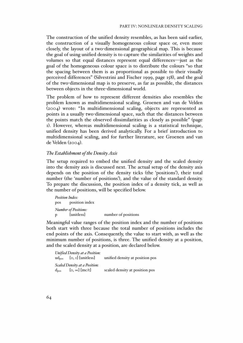
The construction of the unified density resembles, as has been said earlier, the construction of a visually homogeneous colour space or, even more closely, the layout of a two-dimensional geographical map. This is because the goal of using unified density is to capture the similarities of weights and volumes so that equal distances represent equal differences—just as the goal of the homogeneous colour space is to distribute the colours “so that the spacing between them is as proportional as possible to their visually perceived differences” (Silvestrini and Fischer 1999, page 158), and the goal of the two-dimensional map is to preserve, as far as possible, the distances between objects in the three-dimensional world.

The problem of how to represent different densities also resembles the problem known as multidimensional scaling. Groenen and van de Velden (2004) wrote: “In multidimensional scaling, objects are represented as points in a usually two-dimensional space, such that the distances between the points match the observed dissimilarities as closely as possible” (page 1). However, whereas multidimensional scaling is a statistical technique, unified density has been derived analytically. For a brief introduction to multidimensional scaling, and for further literature, see Groenen and van de Velden (2004).

The Establishment of the Density Axis

The setup required to embed the unified density and the scaled density into the density axis is discussed next. The actual setup of the density axis depends on the position of the density ticks (the ‘positions’), their total number (the ‘number of positions’), and the value of the standard density. To prepare the discussion, the position index of a density tick, as well as the number of positions, will be specified below.

Position Index:pos+ position index

Number of Positions:p+ [unitless]+ + number of positions

Meaningful value ranges of the position index and the number of positions both start with three because the total number of positions includes the end points of the axis. Consequently, the value to start with, as well as the minimum number of positions, is three. The unified density at a position, and the scaled density at a position, are declared below.

Unified Density at a Position:udpos+ [0, 1] [unitless]+ unified density at position pos

Scaled Density at a Position:dpos+ [0, ∞] [mc/t]+ + scaled density at position pos


64

The formulas to achieve an equidistant distribution of density ticks along the density axis are given next. The first formula is for an equidistant dis-tribution of the unified density ticks, while the second formula is for the equidistant distribution of scaled density ticks.

Unified Density at a Position as a Function of Position:if+ pos = 1+ + + then udpos = 0elseif+ 1 < pos < p+ + + then udpos = (pos – 1)/(p – 1)elseif+ pos = p+ + + then udpos = 1

Scaled Density at a Position as a Function of Position:if+ pos = 1+ + + then dpos = 0elseif+ 1 < pos ≤ 1 + (p – 1)/2+ then dpos = sdc (2pos – 2)/(p – 1)elseif+ 1 + (p – 1)/2 < pos < p+ then dpos = sdc (p – 1)/(2p – 2pos)elseif+ pos = p+ + + then dpos = ∞

Two sample setups can be seen in Figure 15 below. Having defined the leg-end in the upper part of the figure, the first setup is for a scaled density with 13 positions and a standard density of 6 cubic metres per tonne, and the second density setup is for a unified density with 13 positions. Hence, the first setup is dubbed ‘scaled density (13; 6)’, while the second setup is dubbed ‘unified density (13)’. Note that the setup for the unified density does not depend on the value of the standard density since the unified den-sity is ‘abstract’.

Further examples of scaled density setups are given in the Figures 16 and 17 on Page 66. Figure 16 shows various scaled densities with an even number of positions, and Figure 17 shows various scaled densities with an odd num-ber of positions. It should be noted that some setups are for different stan-dard densities: the first setup in Figure 16, for example, is for a standard density of 1 cubic metre per tonne, while the second setup in the same fig-ure is for a standard density of 5 cubic metres per tonne.

XIV

0 1 32 54 76 98 121110

3.00

2.50

2.00

1.50

1.00

0.50

0.00

Rat

e [e

uro/

chkg

]


13 1514 1716 1918 2120 242322 25 2726 36… !…

0 1/12 1/41/6 5/121/3 7/121/2 3/42/3 111/125/6

0 1 32 54 7.26 129 !3618

0

3.00

2.50

2.00

1.50

1.00

0.50

0.00

Unified Density [unitless]

Rat

e [e

uro/

chkg

]


Elements

0

! 36

0 1/6 3/6 5/62/6 4/6 6/6

1/3 2/3 4/31 5/3

4/3

5/1000

3/1000

0

1/1000

6/1000

4/1000

2/1000

1

2/3

1/3

0

Weight [kg]

Chargeable Weight of Zero Density [chkg]Volum

e [mc]

Cha

rgea

ble

Wei

ght o

f Inf

inite

Den

sity

[chk

g]

Chargeable weight density scaling (standard density = 6 mc/1000 kg)

2Density* [mc/1000 kg]

12 7.218 9 65

3

0

1

4

2

!"#$%&'(

0 1/3 2/3 4/31 5/3

4/3

1

2/3

1/3

0

Chargeable Weight of Zero Density [chkg]

Cha

rgea

ble

Wei

ght o

f Inf

inite

Den

sity

[chk

g]

Domains, gravity centers and the standard density

2

vc/wc " D

ensity " 0

! " Density > vc/wc

vc/wc

G

ED

CBA

F

H

Domain Gravity Centers

1 2 43Domains (Clusters)

Elements

cb fea d g h i j k l m

1 2 43Domains (Clusters)

Domain Gravity Centers

!"#$%&'(

stan

dard

den

sity

: 6 m

c pe

r 100

0 kg

1)

Uniform density domains with chargeable weight density scaling1)

##

##

Disparate density domains without density scaling1)

2)

Elements

cb e f kh i j l mgda

dens

ity o

f dom

ain

grav

ity c

ente

r is

inde

term

inat

e2)

stan

dard

den

sity

: 6 m

c pe

r 100

0 kg

1)

pi-i2 pi-i1 p

Position, Scaled Density [mc/t], and Unified Density [unitless]

Des

crip

tion

Figure 15: Construction and legend of the density scalings

10

position

set of positions

scaled density

unified density

!0 pi-i1dpi-i2d3d2d

1 … …32

ds

1/23ud2ud

0 1/12 1/41/6 5/121/3 7/12

unified density

1/2 3/42/3 111/125/6

0 1 32 54 7.26 129 !3618


positionud


positiond

stan

dard

den

sity

in c

ubic

met

res

per t

onne

1)nu

mbe

r of p

ositi

ons

2)

w

# 0.66

# 0.66

# 0.66

# 0.66

# 0.66# 0.66

# 0.66no

2040

60

80

100

120

140

%sl

…

d (sl)

6.6

6.0

5.4

4.8

4.23.6

3.0

v (sl)

0.5

0.60.7

0.8

0.9

1.0

1.1

w

1

11

1

1

1

1

…

d (sl)

19.8

18.0

16.2

14.4

12.610.8

9.0 !

!

!

!

!

!

!

…

d (sl) w

0

00

0

0

0

0

v (sl)

2.2

2.0

1.8

1.6

1.41.2

1.0 3000

36004200

4800

5400

6000

6600

(sl)D

3000

36004200

4800

5400

6000

6600

(sl)D r (sl)

3.75

# 3.12# 2.67

# 2.34

# 2.08

# 1.87

# 1.70

r (sl)

3.75

# 3.12# 2.67

# 2.34

# 2.08

# 1.87

# 1.70

3000

30003000

3000

3000

3000

3300

(sl)Dr (sl)

3.75

3.75

3.75

3.753.75

3.75

# 3.40

v (sl)

1.0

1.21.4

1.6

1.8

2.0

2.2)"*(

1)

2)

scaled density

(13 )1)

(13 ; 6 )2)1)


65

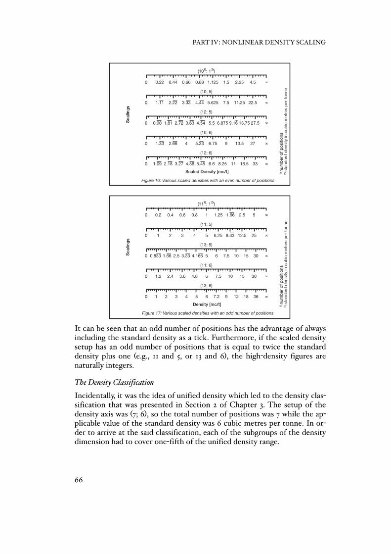
It can be seen that an odd number of positions has the advantage of always including the standard density as a tick. Furthermore, if the scaled density setup has an odd number of positions that is equal to twice the standard density plus one (e.g., 11 and 5, or 13 and 6), the high-density figures are naturally integers.

The Density Classification

Incidentally, it was the idea of unified density which led to the density clas-sification that was presented in Section 2 of Chapter 3. The setup of the density axis was (7; 6), so the total number of positions was 7 while the ap-plicable value of the standard density was 6 cubic metres per tonne. In or-der to arrive at the said classification, each of the subgroups of the density dimension had to cover one-fifth of the unified density range.

Density [mc/t]

Density [m

c/t]

Density [mc/t]3)

…

pi-i2 pi-i1 p

11.9 17.8 23.8 71.535.70 6.50 7.957.15 10.28.94 !14.3

10.214.3

Density [mc/t]

Figure 17: Various scaled densities with an odd number of positions

XIII

0 1 32 54 7.2

(11; 5)

(13; 5)

(11; 6)

(13; 6)

6 129 !3618

Sca

lings

0 0.2 0.60.4 0.8 1.251 2.51.66 !5

0 1.2 3.62.4 64.8

6.25 12.5 25

7.5 1510 !30

0 1 32 54 !

0 0.833 2.51.66 4.1663.33 65 107.5 !3015

8.33

Scaled Density [mc/t]

Figure 16: Various scaled densities with an even number of positions

0 1.09 3.272.18 5.454.36 6.6

(10; 5)

(12; 5)

(10; 6)

(12; 6)

118.25 !3316.5

Sca

lings

0 1.125 2.251.5 !4.5

0 4

5.625 11.25 22.5

6.75 13.59 !27

0 !

0 0.90 2.721.81 4.543.63 5.5 9.166.875 !27.513.75

7.5

1.33 2.66 5.33

1.11 2.22 3.33 4.44

0.880.660.440.22

kilogram and liter density scaling (6; 13)

Non-chargeable weight density scalings with an odd number of positions

Sca

lings

3.50 4.66 5.25 10.25.830 0.58 1.751.16 2.912.33 !4.08

logarithmic with base 2 density scaling (6; 13)

1 2.8221.41 85.654 11. 45.3222.16 64

logarithmic density scaling (6; 13)

1 5.623.161.77 31.17.10 56. 562.316.177.100 1000

0 1 32 54 7

no density scaling (6; 13)

6 98 121110

0 1/3 2/3 4/31 5/3

4/3

! 07.156.507.95

8.9411.917.835.723.871.5

1

2/3

1/3

0

Weight [kg]

Volu

me

[mc]

Kilogramm and cubic meter density scaling

2

Position and Density [mc/t]

Des

crip

tion

Construction and legend of non-chargeable weight density scalings

10100 10…

…

…pi-i1dpi-i2dpositiond3d2d exp

220 … …pi-i1dpi-i2d3d2d exp

position

set of positions

base units density scaling

logarithmic with base 2 density scaling

logarithmic density scaling

pi-i2 pi-i1 p

0

12… …

…6/12 6/76/8 6/6

1/3 2/3 4/31 5/3

4/3

5/1000

3/1000

0

1/1000

6/1000

4/1000

2/1000

1

2/3

1/3

0

Weight [kg]


Volume [m

c]

Cha

rgea

ble

Wei

ght o

f Inf

inite

Den

sity

[chk

g]

2

Density [mc/t]

78 65

3

0

1

4

2

0 …

no density scaling

21

!0 … …pi-i1dpi-i2d3d2d

1 … …32

positiond

positiond

positiond

0 2

8

6

4

2

0

Weight [kg]

Volu

me

[lite

r]

Kilogramm and liter density scaling

00.581.161.752.332.913.504.084.665.255.83

4 86 10 12

!

10.2

0

! 36

0 1/6 3/6 5/62/6 4/6 6/6

1/3 2/3 4/31 5/3

4/3

5/1000

3/1000

0

1/1000

6/1000

4/1000

2/1000

1

2/3

1/3

0

Weight [kg]


Volume [m

c]

Cha

rgea

ble

Wei

ght o

f Inf

inite

Den

sity

[chk

g]

2

12 7.218 9 65

3

0

1

4

2

2)

appr

oxim

ated

2)

2)

!

0

stan

dard

den

sity

in c

ubic

met

res

per t

onne

1)nu

mbe

r of p

ositi

ons

2)st

anda

rd d

ensi

ty in

cub

ic m

etre

s pe

r ton

ne1)

num

ber o

f pos

ition

s2)

appr

oxim

ated

3)

(11 ; 1 )2)1)

stan

dard

den

sity

: 6 c

ubic

met

ers

per t

on1)

stan

dard

den

sity

: 6 c

ubic

met

ers

per t

on1)

stan

dard

den

sity

: 6 c

ubic

met

ers

per t

on1)

1)

1)

No density scaling1)

Chargeable weight density scaling 1)

scale

scale

Density [mc/t]

appr

oxim

ated

2)

kilogram and cubic meter density scaling (6 ; 13 )2)1)

stan

dard

den

sity

in c

ubic

met

ers

per t

on1)

num

ber o

f pos

ition

s2)

(10 ; 1 )2)1)

stan

dard

den

sity

: 6 c

ubic

met

ers

per t

on1)


66

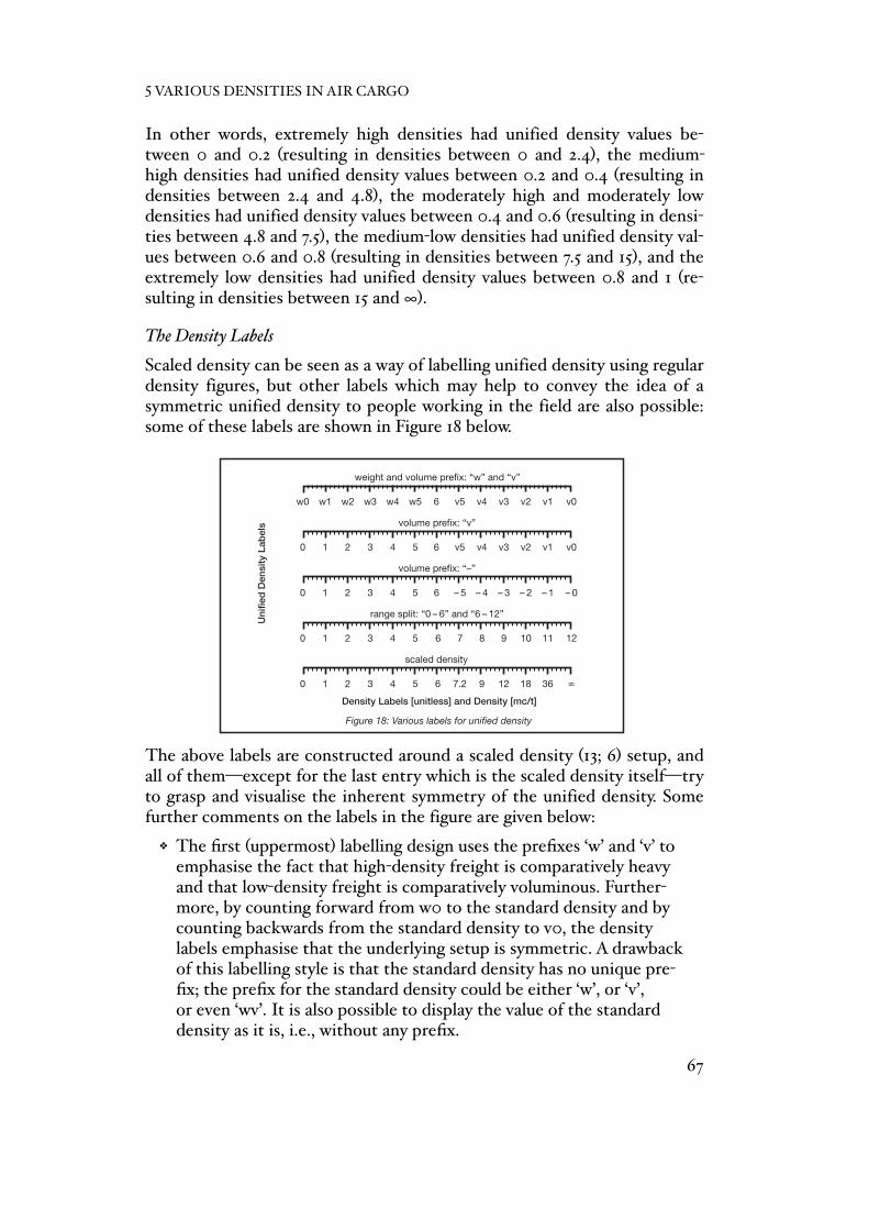
In other words, extremely high densities had unified density values be-tween 0 and 0.2 (resulting in densities between 0 and 2.4), the medium-high densities had unified density values between 0.2 and 0.4 (resulting in densities between 2.4 and 4.8), the moderately high and moderately low densities had unified density values between 0.4 and 0.6 (resulting in densi-ties between 4.8 and 7.5), the medium-low densities had unified density val-ues between 0.6 and 0.8 (resulting in densities between 7.5 and 15), and the extremely low densities had unified density values between 0.8 and 1 (re-sulting in densities between 15 and ∞).

The Density Labels

Scaled density can be seen as a way of labelling unified density using regular density figures, but other labels which may help to convey the idea of a symmetric unified density to people working in the field are also possible: some of these labels are shown in Figure 18 below.

The above labels are constructed around a scaled density (13; 6) setup, and all of them—except for the last entry which is the scaled density itself—try to grasp and visualise the inherent symmetry of the unified density. Some further comments on the labels in the figure are given below:

❖ The first (uppermost) labelling design uses the prefixes ‘w’ and ‘v’ to emphasise the fact that high-density freight is comparatively heavy and that low-density freight is comparatively voluminous. Further-more, by counting forward from w0 to the standard density and by counting backwards from the standard density to v0, the density labels emphasise that the underlying setup is symmetric. A drawback of this labelling style is that the standard density has no unique pre-fix; the prefix for the standard density could be either ‘w’, or ‘v’, or even ‘wv’. It is also possible to display the value of the standard density as it is, i.e., without any prefix.

estsla

estslaamaxsl

critical

qslqsl

dsl

v sl

wsl


stowage loss*

Den

sity

Mix

of T

wo

Item

s [%

]

Uni

fied

Den

sity

Lab

els

0 1 32 54

7.2 6 void

void6

12 9! 36 18

200

166

133

100

Density [mc/t]

Density [mc/t]


–1 –.833 –.5–.66 –.166–.33 0 void


!"


Varia

ble

density withstowage

loss*

revenue

weight

revenue

effectivedemand*


volume withstowage

loss*

weight

revenue


stowage loss*

effectivedemand*

effectiverate*

rasl

–>



Varia

ble

wc[kg/chkg]

tc[kg/t]

chtc[chkg/cht]

tc[kg/t]

tc[kg/t]

tc[kg/t]


ds[mc/t]

vc[mc/cht]

ds[mc/t]

chtc[chkg/cht]

chtc[chkg/cht]

chtc[chkg/cht]

–> derivedinitial



–> derivedinitial


Varia

ble

revenue[euro]

revenue[euro]


volume*[mc]

volume*[mc]

weight[kg]

revenue[euro]



rate*[euro/chkg]


density*[mc/t]

weight[kg]

–> derivedinitial


Properties

Varia

ble

revenue[€]

revenue[€]


volume[mc]

volume[mc]

weight[kg]

revenue[€]

weightcoefficient

[chkg/chkg]


rate[€/chkg]

volumecoefficient

[chkg/chkg]

density[mc/t]

weight[kg]

0 1 32 54 7.2

scaled density

6 129 !3618

0 1 32 54 7

range split: “0 – 6” and “6 – 12”

6 98 121110

w0 w1 w3w2 w5w4 v5


6 v3v4 v0v1v2

0 1 32 54 v5


6 v3v4 v0v1v2

0 1 32 54 – 5


6 – 3– 4 – 0– 1– 2




optimise …


7sl6sl5sl4sl3sl2sl


rejectconfirm

fp mpbc


7sl6sl5sl4sl3sl2sl


fp mpbc

Sto

wag

e Lo

ss R

ange

s

sdc

0 = 1sl0 = 1sl

sdc

aa

a

a

a

amaxsl estsla


67

❖ The second labelling approach uses the prefix ‘v’ only. This is possible because high-density values are equal to the values of the regular density. Note that even though only one prefix is used, the symmetry of the labelling is readily apparent by looking at the figures.

❖ The third labelling option uses positive numbers for high densities and negative numbers for low densities. The advantage of this labelling style is that it does not require an alphanumeric display. Hence, it might be possible to use the graphical features of common standard software to display the density labels. However, it might prove impossible to display high and low densities in the same graph since ordinary software cannot handle a ‘broken’ abscissa. It seems also problematic to assign different density values to ‘0’ and ‘– 0’.

❖ The fourth approach, the range split, tries to avoid the drawbacks of the afore option by counting the high densities from zero to the standard density, and the low densities from the standard density to a value which is double the standard density. In doing so, the high-density values are again equal to the values for the regular density while the low-density figures are in a somewhat ‘disguised’ symmetry. The labels for low densities are, however, not equal to the values of the regular density—which could be quite misleading. It is, forexample, not immediately clear whether the label ‘12’ in the fourth option in Figure 18 denotes a regular density or not (it does not: the density label ‘12’ denotes an infinite density). Nonetheless, such density labels can be easily displayed with the graphical features of common standard software. It might therefore be an option to display the unified density using this labelling but train the users accordingly.

Overall, the first option, using the ‘w’ and ‘v’ prefixes, appears to be the most versatile of the labels suggested in Figure 18. Thus, there are essen-tially three choices for displaying the unified density: the ‘w and v’ labelling of the density, the scaled density, and the unified density itself.

The Standard Density, the Unified Density, and the Chargeable Weight

The relationships between the unified density, the standard density, and the chargeable weight are illustrated in Figure 19. The figure also shows the precedence of the variables and the flow of calculations.


68

In order to calculate the density of an item, to give an example, it is neces-sary to know its unified density as well as the value of the standard density.

The Unified Density and the Extended Set

The unified density is seen as a natural extension of the extended set of de-rived air cargo properties (see Figure 20).

Having added the unified density, the extended set now contains the initial set of air cargo properties, the derived air cargo properties, the density, and the unified density.



1 5.623.161.77 31.17.10 56. 562.316.177.100 1000

… pi-i2 pi-i1 p0 …

keine Skalierung

21 positiond

0 1 32 54 7


6 98 121110



0 1 32 54 7.2

(5; 11)

(5; 13)

(6; 11)

(6; 13)

6 129 !3618

Ska

lieru

ngen

0 0.2 0.60.4 0.8 1.251 2.51.66 !5

0 1.2 3.62.4 64.8

6.25 12.5 25

7.5 1510 !30

0 1 32 54 !

0 0.833 2.51.66 4.1663.33 65 107.5 !3015

8.33



0 1.09 3.272.18 5.454.36 6.6

(1 ; 10 )

(5; 10)

(5; 12)

(6; 10)

(6; 12)

118.25 !3316.5

Ska

lieru

ngen

0 1.125 2.251.5 !4.5

0 4

5.625 11.25 22.5

6.75 13.59 !27

0 !

0 0.90 2.721.81 4.543.63 5.5 9.166.875 !27.513.75

7.5

1.33 2.66 5.33

1.11 2.22 3.33 4.44

0.880.660.440.22


Bes

chre

ibun

g



3)

2)1)

Sta

ndar

d–Vo

lum

enge

wic

ht1)

Anz

ahl v

on P

ositi

onen

2)S

tand

ard–

Volu

men

gew

icht

1)

Anz

ahl v

on P

ositi

onen

2)

(1 ; 11 )2)1)


Set an Positionen

1 … …32


2)1)

circ

a A

ngab

en3)

Sta

ndar

d–Vo

lum

enge

wic

ht1)

Anz

ahl v

on P

ositi

onen

2)

pi-i2 pi-i1 p


Bes

chre

ibun

g un

d S

kalie

rung


10

position

Set an Positionen



!0 pi-i1dpi-i2d3d2d

1 … …32

ds

1/23ud2ud

0 1/12 1/41/6 5/121/3 7/12


1/2 3/42/3 111/125/6

0 1 32 54 7.2


6 129 !3618


positionud


positiond

Sta

ndar

d–Vo

lum

enge

wic

ht1)

Anz

ahl v

on P

ositi

onen

2)

2)1)

XVII





d[mc /t ]

Chargeable

[chkg ]Weight cw

[kg ] [mc ]

0.0060.601.000.60101

0.0061.001.001.0061

0.0041.000.661.0041

0.0021.000.331.00210.0011.000.161.00110.0001.000.001.0001

0.0051.000.831.0051

0.0060.661.000.6691

0.0031.000.501.0031

0.0060.851.000.85710.0060.751.000.7581

………………0.0060.001.000.00!1

"

"

"

"

"

"

"

"

–>



Varia

ble



volume[mc]

standarddensity

[mc/t]


weight[kg]

weight[kg]

–>



Varia

ble


volume[mc]

volume[mc]

standarddensity

[mc/t]

weight[kg]

weight[kg]

–> derivedinitial


Properties

Varia

ble

cost[€]

cost[€]


volume[mc]

volume[mc]

weight[kg]

cost[€]

weightcoefficient

[chkg/chkg]


unit cost[€/chkg]

volumecoefficient

[chkg/chkg]

density[mc/t]

weight[kg]

density[mc/t]


unifieddensity

[unitless]

scaleddensity[mc/t]

or

volume[mc]

density[mc/t]



u > 0ij x > 0ij

XVIII


Com

plem

enta

ry S

lack

ness

Con

ditio

n


u = 0ij

s > 0ij p = 0ij

u = 0ijs = 0ij

p > 0ij

x = 0ijp = 0ij

p = 0iju =ij

x = 0ij

ijijp = 0 ! x

ijijp = x = 0

u = 0 ! sijij


u " 0 < sijij

x =ij Dij

0 ! x !ij Dij


0 10 20 30 40 6050

4.00

3.50

3.00

2.50

2.00

0.50

1.50

1.00

0.00


Rat

e [e

uro/

chkg

]

Wk

demandforecast


BCxBCx


0 10 20 30 40 6050

4.00

3.50

3.00

2.50

2.00

0.50

1.50

1.00

0.00


Rat

e [e

uro/

chkg

]

Wk

demandforecast


BCoptr

minBCr

BCr

WkBCD– BCw

optmax

0 1 2 43 65

4

3

2

1

0

Weight [t]

Volu

me

[mc]


# m

c/t

4 m

c/t

2 m

c/t

1.33

mc/

t

1 mc/

t

0.8 mc/t

0 mc/t

0.66 mc/t

1)

stan

dard

den

sity

(das

hed)

: 6 c

ubic

met

res

per t

onne

1)


0 20 40 60 80 120100

4.00

3.50

3.00

2.50

2.00

0.50

1.50

1.00

0.00


Rat

e [€

/chk

g]

–> derivedinitial


Properties

Varia

ble

revenue[€]

revenue[€]


volume[mc]

weight[kg]

revenue[€]

weightcoefficient

[chkg/chkg]


rate[€/chkg]

volumecoefficient

[chkg/chkg]


weight[kg]

0 100 200 400300 500

400

300

200

100

0


Rev

enue

[€]

600


100r

500+r

500r

R

Density [mc/t]

Rat

e [€

/chk

g]


s

disl dis

u

risu

risl

domaindemandqis

i

disdomaindensity

risdomain

ratex

x

x

x

x

x x

xx

x

x

density[mc/t]

volume[mc]

m

np

u

NW(s, x) NE(s, u)

SW(p, x) SE(p, u)

D =ij 0x =ij

m

ijijp " 0 = xn


nn

s>=0

s=0

u>=0


69

5.3 Contribution

The regular density (or the inverse regular density in pounds per cubic feet) is currently the prevailing term used to describe a volume-to-weight ratio in air cargo (see, for example, the extensive use of the inverse regular density in Radnoti 2002, pages 89ff.). However, the direct use of the regular density has, as has been shown in Section 1 of Chapter 5, several disadvantages: the contribution of this chapter is therefore considered to be the critical anal-ysis of the regular density (i.e., the density ‘as is’), the introduction of the unified density, the scaled density, a review of various set-up options for use with the scaled density, the density labels, and a density classification based on the unified density.

The author of this dissertation is unaware of any earlier literature that con-siders the unified density, the scaled density, or any of the other aforemen-tioned contributions. The concepts of unified density and scaled density are patent pending in Germany, the European Union, and elsewhere.

Having introduced the unified density, it is also possible to declare the in-dependent variables in air cargo. From an economic point of view, the independent variables are not, as has been stated by Pak (2005, page 128), the weight of the freight, its volume (or density), and the profit per weight, but the freight’s unified density, its chargeable weight, and its rate per chargeable weight. This is because the economic decisions to confirm or reject the booking requests are most closely linked to the values of these variables.

The final part of the dissertation is about the three central parts of any Revenue Management System: forecasting, optimisation, and control.


70


71

PART V: FORECASTING, OPTIMISATION, AND CONTROL

6 Segment Demand (Forecast)

Since future booking requests are rarely known in advance, the segment demand has to be forecast in order for a Cargo Revenue Management Sys-tem to make effective use of the instruments that are available to increase the revenue of a flight. Nevertheless, this chapter is essentially not about forecasting segment demand, but about what exactly the demand is, and about determining demand aggregates that may be easier to forecast than the individual future booking requests.

In the first section of this chapter, the segment demand and the demand distribution will be discussed (some demand-distribution graphs will also be provided). The rate-density domains, the gravity centres, and the aggre-gated demand will then be discussed in the second section, and the third section concerns demand aggregation and its requirements. This third sec-tion includes a discussion of several aggregation schemes, it lists the pros and cons of forecasting an aggregate, and it includes a discussion about the optimum number and the best size of the domains. The fourth section considers the rate-density grid and its set-up. The chapter ends by assessing its contribution to knowledge in this field.

6.1 Segment Demand and Demand Distribution

In order to optimise a flight’s revenue and to achieve effective booking re-quest control, it is not enough to know the overall quantity of the future demand: the demand has to be differentiated according to various criteria. More specifically, it is essential that the demand be differentiated by all the criteria which have a significant impact on the flight revenue. In air cargo, these criteria are the routing of the demand (i.e., by segment), as well as its rate and its density.

The Segment Demand, its Density, and its Rate

The segment demand has already been defined as the joint chargeable weight of those future bookings which will be requested for a particular flight segment during the remaining booking period. Next, a further differ-entiation will lead to a segment demand that is characterised by a specific density and a certain rate.

73

The Demand Distribution

In general, the booking requests are not randomly distributed within the rate-density space but follow certain ‘norms’:

❖ The empirical distribution of the unified density of the booking requests is symmetrically centred on the standard density. This pattern reflects the observation that high-density bookings seem to be as frequently requested as low-density ones.

❖ The empirical distribution of the unified density of booking requests resembles the bell-shaped Normal distribution, with the standard density as the mean. This pattern is linked to the observation that most of the bookings requested have the standard density, or a density which is close to the standard density. Moreover, experience shows that extreme densities are requested only occasionally.

❖ A greater number of—and larger—bookings will be requested at a lower rate, but no (or very few) bookings will be requested below a certain rate level. This pattern reflects three observations. The first observation is that large shipments are already priced competitively because of the chargeable weight breakpoints and the negotiation power of the customers. The second observation is that the lower the rate, the more bookings that will be requested, and the third observation is that rates below a certain level are simply not made available by the carriers’ pricing departments.

The above norms are, of course, of a generic nature. They can (and many times will) be proven wrong on particular flight segments, but the author’s overall experience based on the observation of thousands of flights at a major European cargo airline is that the rate and density distribution of the segment demand follows the given patterns, at least in general, in the absence of special influences, and when many bookings will be requested.

To summarise, Figure 21 on Page 75 shows the typical rate and density dis-tribution of the real-world demand in the air cargo business. The shades of grey in the figure reflect the likelihood of a booking being requested within the circumscribed rate and density ranges. Light grey, for example, means that few bookings will be requested with the given rate and density, where-as dark grey means that it is likely that many bookings will be requested with that combination. If an area is white, it is because there is simply no demand with that rate and density.


74

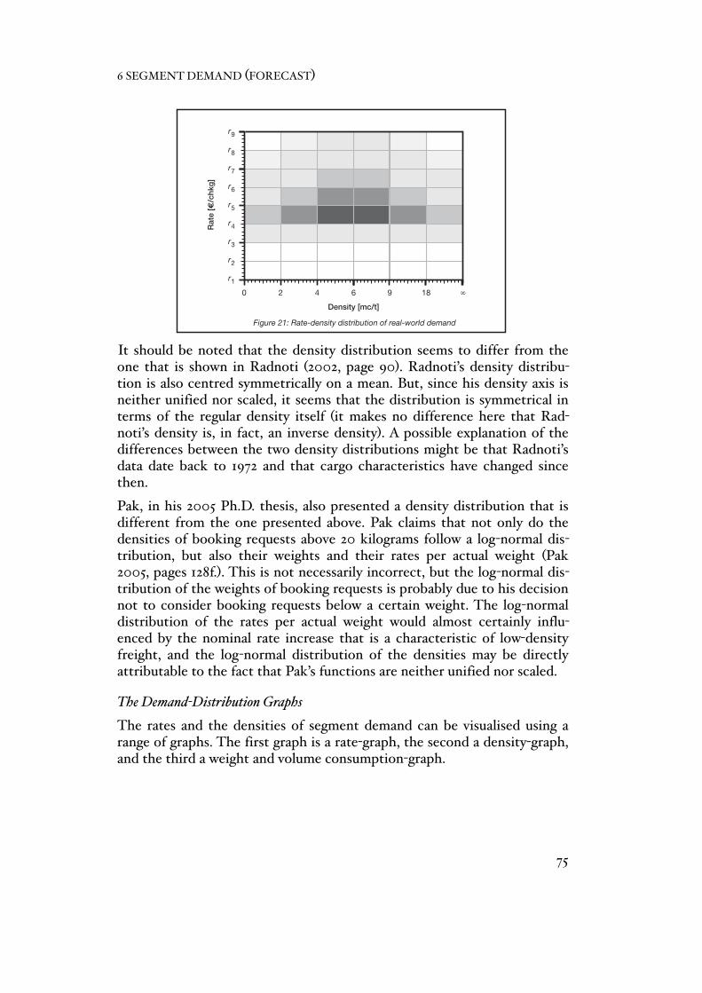
It should be noted that the density distribution seems to differ from the one that is shown in Radnoti (2002, page 90). Radnoti’s density distribu-tion is also centred symmetrically on a mean. But, since his density axis is neither unified nor scaled, it seems that the distribution is symmetrical in terms of the regular density itself (it makes no difference here that Rad-noti’s density is, in fact, an inverse density). A possible explanation of the differences between the two density distributions might be that Radnoti’s data date back to 1972 and that cargo characteristics have changed since then.

Pak, in his 2005 Ph.D. thesis, also presented a density distribution that is different from the one presented above. Pak claims that not only do the densities of booking requests above 20 kilograms follow a log-normal dis-tribution, but also their weights and their rates per actual weight (Pak 2005, pages 128f.). This is not necessarily incorrect, but the log-normal dis-tribution of the weights of booking requests is probably due to his decision not to consider booking requests below a certain weight. The log-normal distribution of the rates per actual weight would almost certainly influ-enced by the nominal rate increase that is a characteristic of low-density freight, and the log-normal distribution of the densities may be directly attributable to the fact that Pak’s functions are neither unified nor scaled.

The Demand-Distribution Graphs

The rates and the densities of segment demand can be visualised using a range of graphs. The first graph is a rate-graph, the second a density-graph, and the third a weight and volume consumption-graph.

–>

6


D

XIX

TransitHandling

(additional flight)

(first flight)

AirTransportation

TransitHandling


Freight Transport

Forw

arde

rA

ir C

argo

Car

rier

Invo

lved

Par

ties Ground


ImportHandling


AirTransportation

ExportHandling

Storage

Consignor Consignee

70 50 1030 10 3080 60 40 020 20

630

180

450

75

105

90

120

270

720

540

360


Weight [t]

Volu

me

[mc]

40

Figure 24: Weight and volume consumption-graph of a segment

70 50 1030 10 3080 60 40 020 20

105

75

45

15

120

90

60

30

0

Weight [kg]


Volume [m

c]

Cha

rgea

ble

Wei

ght [

chkg

]

40

Chargeable weight density scaling

Volume [mc]

Wei

ght [

chkg

]

90

75

60

15

45

30

0

120

105

Reduced capacities are leading to higher bid prices

0 10 20 30 40 6050

4.00

3.50

3.00

2.50

2.00

0.50

1.50

1.00

0.00

Supply and Demand [t]

Rat

e [e

uro/

kg]

D

r

W90%W100%W80%W70%

bpw70/80%

bpw90%

bpw100%

30

60

45

15

0

high density low densityC

BA

0

90


Rat

e [e

uro/

chkg

]

A non-overlapping rate-density domain

j

0 10.5udijl udij

u

riju

rijl i

x

x

x

x x x

xx

x

x

0 2 4 96 !18

4.00

3.50

3.00

2.50

2.00

0.50

1.50

1.00

0.00

Density [mc/t]

Rat

e [e

uro/

chkg

]

Rate-density grid of a real world flight

1 2

31 343332

25 3029282726

21 242322

15 2019181716

9 1413121110

3 87654

1

Figure 23: Density-graph of a segment

0 20 40 60 80 120100

!

12

36

7.2

18

9

1

2

5

4

3

0


Den

sity

[mc/

t]

0 2 4 96 !18

Density [mc/t]

Rat

e [€

/chk

g]

Figure 21: Rate-density distribution of real-world demand

9r

8r

7r

6r

5r

4r

3r

2r

1r

6 SEGMENT DEMAND (FORECAST)

75

The rate-graph shows the cumulative segment demand in chargeable kilo-grams as a function of its rate, and an example is given in Figure 22 below.

Complementing the rate-graph is the density-graph. The density-graph shows the cumulative segment demand as a function of scaled density as il-lustrated in Figure 23 below.

The density-graph shows, like the rate-graph, only one dimension, that is, the density-graph does not take the rate of the segment demand into ac-count, in the same way as the rate-graph does not take account of density. Both, however, do offer an informative view of the structure of the rates and the densities of the demand.

A more informative view of the density distribution is provided by the next graph (see Figure 24 on Page 77). This weight and volume consumption-graph gives an intuitive impression of the benefits of segment demand with a non-standard density.

u > 0ij x > 0ij

XVIII


Com

plem

enta

ry S

lack

ness

Con

ditio

n


u = 0ij

s > 0ij p = 0ij

u = 0ijs = 0ij

p > 0ij

x = 0ijp = 0ij

p = 0iju =ij

x = 0ij

ijijp = 0 ! x

ijijp = x = 0

u = 0 ! sijij


u " 0 < sijij

x =ij Dij

0 ! x !ij Dij


0 10 20 30 40 6050

4.00

3.50

3.00

2.50

2.00

0.50

1.50

1.00

0.00


Rat

e [e

uro/

chkg

]

Wk

demandforecast


BCxBCx


0 10 20 30 40 6050

4.00

3.50

3.00

2.50

2.00

0.50

1.50

1.00

0.00


Rat

e [e

uro/

chkg

]

Wk

demandforecast


BCoptr

minBCr

BCr

WkBCD– BCw

optmax

0 1 2 43 65

4

3

2

1

0

Weight [t]

Volu

me

[mc]


# m

c/t

4 m

c/t

2 m

c/t

1.33

mc/

t

1 mc/

t

0.8 mc/t

0 mc/t

0.66 mc/t

1)

stan

dard

den

sity

(das

hed)

: 6 c

ubic

met

res

per t

onne

1)


0 20 40 60 80 120100

4.00

3.50

3.00

2.50

2.00

0.50

1.50

1.00

0.00


Rat

e [€

/chk

g]

–> derivedinitial


PropertiesVa

riabl

e

revenue[€]

revenue[€]


volume[mc]

weight[kg]

revenue[€]

weightcoefficient

[chkg/chkg]


rate[€/chkg]

volumecoefficient

[chkg/chkg]


weight[kg]

0 100 200 400300 500

400

300

200

100

0


Rev

enue

[€]

600


100r

500+r

500r

R

Density [mc/t]

Rat

e [€

/chk

g]


s

disl dis

u

risu

risl

domaindemandqis

i

disdomaindensity

risdomain

ratex

x

x

x

x

x x

xx

x

x

density[mc/t]

volume[mc]

m

np

u

NW(s, x) NE(s, u)

SW(p, x) SE(p, u)

D =ij 0x =ij

m

ijijp " 0 = xn


nn

s>=0

s=0

u>=0

–>

6


D

XIX

TransitHandling

(additional flight)

(first flight)

AirTransportation

TransitHandling


Freight Transport

Forw

arde

rA

ir C

argo

Car

rier

Invo

lved

Par

ties Ground


ImportHandling


AirTransportation

ExportHandling

Storage

Consignor Consignee

70 50 1030 10 3080 60 40 020 20

630

180

450

75

105

90

120

270

720

540

360


Weight [t]

Volu

me

[mc]

40


70 50 1030 10 3080 60 40 020 20

105

75

45

15

120

90

60

30

0

Weight [kg]


Volume [m

c]

Cha

rgea

ble

Wei

ght [

chkg

]

40


Volume [mc]

Wei

ght [

chkg

]

90

75

60

15

45

30

0

120

105


0 10 20 30 40 6050

4.00

3.50

3.00

2.50

2.00

0.50

1.50

1.00

0.00


Rat

e [e

uro/

kg]

D

r

W90%W100%W80%W70%

bpw70/80%

bpw90%

bpw100%

30

60

45

15

0


BA

0

90


Rat

e [e

uro/

chkg

]


j

0 10.5udijl udij

u

riju

rijl i

x

x

x

x x x

xx

x

x

0 2 4 96 !18

4.00

3.50

3.00

2.50

2.00

0.50

1.50

1.00

0.00

Density [mc/t]

Rat

e [e

uro/

chkg

]


1 2

31 343332

25 3029282726

21 242322

15 2019181716

9 1413121110

3 87654

1


0 20 40 60 80 120100

!

12

36

7.2

18

9

1

2

5

4

3

0


Den

sity

[mc/

t]

0 2 4 96 !18

Density [mc/t]

Rat

e [€

/chk

g]


9r

8r

7r

6r

5r

4r

3r

2r

1r


76

It shows the cumulative weight and volume consumption of the demand as a function of its density, but it does not take into account the rate of the segment’s demand.

The data shown in the sample graph are as follows: the total future demand is 120,000 chargeable kilograms. Eighty thousand chargeable kilograms of the total are high-density demand, and 40,000 chargeable kilograms are low-density demand. The total weight consumption of the total demand is 105,000 kilograms. Eighty thousand kilograms of the total weight con-sumption are linked to the high-density demand, and 25,000 kilograms of the total weight consumption relate to the low-density demand. The total volume consumption of the total demand is 540 cubic metres. Two hun-dred and forty cubic metres of the total volume consumption are filled with low-density demand, and 300 cubic metres of the total volume con-sumption are filled with high-density demand.

As can be seen in the graph, the volume consumption of the future demand is expressed in cubic metres, the weight consumption of the future demand is expressed in tonnes (or its equivalent in kilograms), and the future de-mand itself is stated in chargeable tonnes (or its equivalent in chargeable kilograms). Furthermore, the value ranges of the expected weight and vol-ume consumptions correspond to the weight and volume equivalents of the total future demand. Thus, if the total demand is 120 chargeable tonnes, the volume range runs from zero to 720 cubic metres, while the weight range runs from zero to 120 tonnes.

The construction approach to the weight and volume consumption-graph is to sort the densities progressively from the centre out, starting with the standard density. High-density demand is shown to the left of the abscissa’s zero reference point (the higher the density, the further it is to the left), and low-density demand is shown to the right of the reference point (the lower the density, the further it is to the right). As a result, the curve has its

–>

6


D

XIX

TransitHandling

(additional flight)

(first flight)

AirTransportation

TransitHandling


Freight Transport

Forw

arde

rA

ir C

argo

Car

rier

Invo

lved

Par

ties Ground


ImportHandling


AirTransportation

ExportHandling

Storage

Consignor Consignee

70 50 1030 10 3080 60 40 020 20

630

180

450

75

105

90

120

270

720

540

360


Weight [t]

Volu

me

[mc]

40


70 50 1030 10 3080 60 40 020 20

105

75

45

15

120

90

60

30

0

Weight [kg]


Volume [m

c]

Cha

rgea

ble

Wei

ght [

chkg

]

40


Volume [mc]

Wei

ght [

chkg

]

90

75

60

15

45

30

0

120

105


0 10 20 30 40 6050

4.00

3.50

3.00

2.50

2.00

0.50

1.50

1.00

0.00


Rat

e [e

uro/

kg]

D

r

W90%W100%W80%W70%

bpw70/80%

bpw90%

bpw100%

30

60

45

15

0


BA

0

90


Rat

e [e

uro/

chkg

]


j

0 10.5udijl udij

u

riju

rijl i

x

x

x

x x x

xx

x

x

0 2 4 96 !18

4.00

3.50

3.00

2.50

2.00

0.50

1.50

1.00

0.00

Density [mc/t]

Rat

e [e

uro/

chkg

]


1 2

31 343332

25 3029282726

21 242322

15 2019181716

9 1413121110

3 87654

1


0 20 40 60 80 120100

!

12

36

7.2

18

9

1

2

5

4

3

0


Den

sity

[mc/

t]

0 2 4 96 !18

Density [mc/t]

Rat

e [€

/chk

g]


9r

8r

7r

6r

5r

4r

3r

2r

1r


77

‘centre’ at the zero reference point of the abscissa, starting with the de-mand that has the standard density (standard density demand is considered to be 50% high-density demand, shown to the left of the reference point, and 50% low-density demand, shown to the right of the reference point).

In general, the weight and volume consumption-graph has four sections: a top-left section (A), a top-right section (B), a bottom-left section (C), and a bottom-right section (D).

The volume consumed by the low-density demand is depicted by the height of Section C (240 cubic metres), and the volume consumed by the high-density demand is shown in Section A (540 – 240 = 300 cubic metres), the weight consumption of the high-density demand is shown by the height of Section B (80 tonnes), and the weight consumed by the low-density demand is shown in Section D (105 – 80 = 25 tonnes). Hence, the volume consump-tion of the high-density demand is on top of the basic volume consumption of the low-density demand, and the weight consumption of the low-density demand is on top of the basic weight consumption of the high-density demand.

From the construction of the graph, it is clear that if all of the demand had a standard density, the curve would be a straight line from the top left cor-ner of Section A to the bottom right corner of Section D. The shape of the curve in Section A is due to the reduced volume consumption of the high-density demand, while the shape of the curve in Section D is due to the reduced weight consumption of the low-density demand.

In the above weight and volume consumption-graph, the reduced volume consumption of the high-density demand leads to accumulated volume sav-ings of 180 cubic metres (720 – 540 cubic metres), while the reduced weight consumption of the low-density demand leads to cumulated weight savings of 15,000 kilograms (120 – 105 tonnes). Both savings are possible because a large part of the demand does not have a standard density.

6.2 Rate-Density Domains

The rate-density domains are defined for each segment, and each rate-density domain covers a certain area of the rate-density continuum. The purpose of using rate-density domains is to categorise the differentiated segment demand and enable its aggregation. This is not a straightforward task; as Pak (2005) wrote on page 115: “How to group the cargo shipments into distinct classes is not trivial.” On page 120, he claimed, “… cargo shipments cannot be categorized into distinct classes”, and on page 113 he wrote, “each cargo shipment is unique”.


78

The Rate-Density Domains of a Segment

The rate-density domains of the segments serve as ‘buckets’ that collect the future booking requests and replace them with as many aggregated vir-tual booking requests as there are rate-density domains that have a positive aggregated demand.

The rate-density domains work as follows: if a future booking is requested for a particular segment, and if it has a rate and a density which fall within the area of a particular domain, the request will qualify as part of that domain’s future demand. Where the future demand consists of several future booking requests, these will be aggregated into one item—the aggre-gated booking request—which has one aggregated rate and one aggregated density.

One of the benefits of setting up several rate-density domains is that the number of domains will usually be less than the number of future bookings that will be requested for a segment. There is, however, a need for a lower limit on the number of domains, or, to put it differently, there is an upper limit on their size. This is because, for the overall success of a Cargo Revenue Management System, it is crucial not only that the number of rate domains is manageable but also that their aggregated rates and densities are still sufficiently detailed to serve as useful input for flight revenue opti-misation.

In order to be able to refer to the rate-density domains of a segment indi-vidually, a domain index is needed. This index is labelled the rate-density domain index and is specified below. With the help of this index and the segment index, it is possible to refer to the individual rate-density domains of a segment.

Rate-Density Domain Index:i0 rate-density domain index

Even though no explicit upper bound has been assigned to the value range of the rate-density domain index, in practice, the most useful number of different rate-density domains per segment is rarely less than 18 and rarely greater than 72. The rationale for the lower bound of 18 domains is that having fewer rate-density domains results in insufficient detail, while the rationale for the upper bound of 72 domains is that increasing the number of domains beyond this limit increases the sparsity of the domains. More will be said about the optimum number of rate-density domains in the third section of this chapter.

Since the rate-density domains are rectangular, the covered area can be described by a simple combination of the lower and upper rate and density limits, with the rate limits defining the rate range of a domain, and the density limits defining its density range. The rate and density limits are detailed on the next page.


79

Lower and Upper Rate Limits of a Rate-Density Domain:rlis0 [0, ∞) [€/chkg]0 lower limit of the rates covered by 0 0 0 0 rate-density domain i of flight segment sruis0 [0, ∞) [€/chkg]0 upper limit of the rates covered by 0 0 0 0 rate-density domain i of flight segment s

Lower and Upper Density Limits of a Rate-Density Domain:dlis0 [0, ∞] [mc/t]0 0 lower limit of the densities covered by 0 0 0 0 rate-density domain i of flight segment sduis0 [0, ∞] [mc/t]0 0 upper limit of the densities covered by 0 0 0 0 rate-density domain i of flight segment s

To be meaningful, the lower rate and density limits have, of course, to be lower than, or equal to, the upper rate and density limits.

The so-called domain incidence coefficients are defined next. The domain incidence coefficients are needed to assign future booking requests to their appropriate domains.

Domain Incidence Coefficient:abis0 {0, 1} [unitless]0 incidence coefficient of booking request b0 0 0 0 on rate-density domain i of flight segment s

Given that the rate-density domains are rectangular, the domain incidence coefficients can be calculated as shown below.

Domain Incidence Coefficient as a Function of Rate and Density:if booking request b is requested on flight segment s, and if the rate is within the rate range of domain i of segment s,and if the density is within the density range of domain i of segment s0 0 0 0 then abis = 10 0 0 0 elseif abis = 0

Special care has to be taken to prevent both overlooking and double-counting future booking requests if a segment has several rate-density domains. More specifically, one has to ensure that each booking request can be assigned to exactly one rate-density domain and that the whole, or at least the relevant, rate-density space is covered by the domains.

The Rate-Density Domain, the Gravity Centre and the Aggregated Demand

To illustrate the concept of demand aggregation, several future booking re-quests, a rate-density domain and the gravity centre of the domain are shown in Figure 25.

The gravity centre is marked by an ‘o’, the rate-density domain is depicted in grey, and the future booking requests are marked by ‘x’. The demand it-self has not been visualised in the figure, but it can be thought of as the third dimension in the three-dimensional space.


80

As can be seen, there are three types of aggregation within a rate-density domain: a demand aggregation, a rate aggregation, and a density aggrega-tion.

An implication of the aggregation is that the aggregated demand is located at the intersection of the aggregated rate and the aggregated density within the two-dimensional area of the domain. This point is also known as the domain’s gravity centre.

The Aggregated Demand of a Rate-Density Domain

The aforementioned aggregates are introduced and declared in more detail below, but formulas will not be presented until the aggregation require-ments have been discussed.

❖ The demand aggregation sums the chargeable weights of future booking requests which are in a particular segment’s domain. The aggregated demand is called the demand of a rate-density domain and is given the symbol qis.

Demand of a Rate-Density Domain:qis0 [0, ∞) [chkg]0 0 demand-to-come of rate-density domain i 0 0 0 0 of flight segment s

The value range of the aggregated demand does not match the value range for the demand of a single booking request because the demand of the rate-density domains can (and often will) be zero, whereas a booking request that has a zero demand is considered an outlier.

u > 0ij x > 0ij

XVIII


Com

plem

enta

ry S

lack

ness

Con

ditio

n


u = 0ij

s > 0ij p = 0ij

u = 0ijs = 0ij

p > 0ij

x = 0ijp = 0ij

p = 0iju =ij

x = 0ij

ijijp = 0 ! x

ijijp = x = 0

u = 0 ! sijij


u " 0 < sijij

x =ij Dij

0 ! x !ij Dij


0 10 20 30 40 6050

4.00

3.50

3.00

2.50

2.00

0.50

1.50

1.00

0.00


Rat

e [e

uro/

chkg

]

Wk

demandforecast


BCxBCx


0 10 20 30 40 6050

4.00

3.50

3.00

2.50

2.00

0.50

1.50

1.00

0.00


Rat

e [e

uro/

chkg

]

Wk

demandforecast


BCoptr

minBCr

BCr

WkBCD– BCw

optmax

0 1 2 43 65

4

3

2

1

0

Weight [t]

Volu

me

[mc]


# m

c/t

4 m

c/t

2 m

c/t

1.33

mc/

t

1 mc/

t

0.8 mc/t

0 mc/t

0.66 mc/t

1)

stan

dard

den

sity

(das

hed)

: 6 c

ubic

met

res

per t

onne

1)


0 20 40 60 80 120100

4.00

3.50

3.00

2.50

2.00

0.50

1.50

1.00

0.00


Rat

e [€

/chk

g]

–> derivedinitial


Properties

Varia

ble

revenue[€]

revenue[€]


volume[mc]

weight[kg]

revenue[€]

weightcoefficient

[chkg/chkg]


rate[€/chkg]

volumecoefficient

[chkg/chkg]


weight[kg]

0 100 200 400300 500

400

300

200

100

0


Rev

enue

[€]

600


100r

500+r

500r

R

Density [mc/t]

Rat

e [€

/chk

g]


s

disl dis

u

risu

risl

domaindemandqis

i

disdomaindensity

risdomain

ratex

x

x

x

x

x x

xx

x

x

density[mc/t]

volume[mc]

m

np

u

NW(s, x) NE(s, u)

SW(p, x) SE(p, u)

D =ij 0x =ij

m

ijijp " 0 = xn


nn

s>=0

s=0

u>=0 6 SEGMENT DEMAND (FORECAST)

81

❖ The rate aggregation calculates the rate of the aggregated demand for a particular segment’s domain. The aggregated rate is called the rate of a rate-density domain and has the symbol ris.

Rate of a Rate-Density Domain:ris0 [0, ∞) [€/chkg]0 rate of rate-density domain i of flight segment s

The value range of the aggregated rate does not match the value range of the rate of a single booking request because the rate of a rate-density domain is a priori not restricted to being greater than zero, i.e., the rate of a domain can be—at least in theory—zero.

Of more practical relevance, however, is the case where the rate of a rate-density domain is indeterminate, something which occurs when the demand of a domain is zero and no default rate has been specified.

❖ The density aggregation calculates the density of the aggregated demand of a particular segment’s domain. The aggregated density is called the density of a rate-density domain and is given the symbol dis.

Density of a Rate-Density Domain:dis0 [0, ∞] [mc/t]0 0 density of rate-density domain i of flight segment s

An alternative to density aggregation is to aggregate unified density. The aggregated unified density is explained below.

❖ Unified density aggregation calculates the unified density of the aggregated demand of a particular segment’s domain. The aggregated unified density is called the unified density of a rate-density domain and has the symbol udis.

Unified Density of a Rate-Density Domain:udis0 [0, 1] [unitless]0 unified density of rate-density domain i 0 0 0 0 of flight segment s

The value ranges of the aggregated density and the aggregated unified den-sity match their respective single booking request value ranges. However, if the aggregated demand of a rate-density domain is zero, and if no default density has been specified (either a regular density or a unified density), both densities are indeterminate.

It was noted earlier in Chapter 5 that either form of density can be used to describe the volume-to-weight ratio of the demand since either can be con-verted into the other. Thus, an adequate representation of the features of the future demand is given either by the demand, the rate, and the density; or by the demand, the rate, and the unified density.


82

6.3 Demand Aggregation

In order to be able to compare a range of aggregation schemes, the require-ments regarding demand aggregation must be considered. The most pro-minent requirement is the quest for linearity, i.e., a demand representation is sought that allows one to ‘add things up’. Once such a demand represen-tation is identified, it becomes viable to suggest not forecasting individual future booking requests but, rather, to forecast their aggregated demand.

The Requirements of Demand Aggregation

The principal requirements regarding demand aggregation of a single rate-density domain are as follows:

❖ The aggregated demand of a single domain should be equal to the total of its individual demands.

❖ The aggregated properties of the aggregated demand of a single domain (e.g., its aggregated rate) should be equal to the total of its weighted individual properties (e.g., equal to the total of the weighted individual rates).

In other words, the demands of the future booking requests should ‘add up’, and the properties of the future booking requests should ‘add up pro-portionally’.

To be able to add up the properties of the future booking requests with their relative weights, weighting factors are needed. The weighting factors denote the future booking requests’ share of the domain’s aggregated demand. The value range of the weighting factors is restricted to non-negative values between zero and one, and the declaration for the weight-ing factor—as well as its definition—are given below.

Weighting Factor of a Booking Request:µbis0 [0, 1] [unitless]0 booking request b’s share of the aggregated 0 0 0 0 demand-to-come of domain i of flight segment s

Weighting Factor of a Booking Request as a Function of Demand:if0 qis = 00 0 0 then µbis is indeterminateelseif0 qis > 00 0 0 then µbis = abis (qb/qis)

Provided the aggregated demand of a rate-density domain is greater than zero, the sum of the weighting factors is equal to one (i.e., ∑b∈Bf µbis = 1). If not, i.e., if the demand is zero, the weighting factors of the future booking requests are indeterminate.

However, there are additional requirements regarding the demand aggrega-tion of a single rate-density domain. These are that the weight, volume, and revenue figures which are obtained using the aggregated properties of the aggregated demand should be consistent with the total weight, volume, and revenue of the individual demands.


83

The Initial Aggregation Scheme

An initial suggestion for calculating the aggregated demand, rate, and den-sity of a domain is to sum the demands in a domain and to proportionally sum the individual rates and densities. In other words:

❖ The aggregated demand of a particular segment’s domain is equal to the sum of its individual demands, i.e., qis = ∑b∈Bf abis qb.

❖ The aggregated rate of a non-zero aggregated demand is equal to the weighted average of the rates of the individual demands or, more precisely, the aggregated domain rate is a linear convex combination of the domain’s individual demand rates: i.e., ris is either equal to ∑b∈Bf µbis rb, or it is indeterminate.

❖ The aggregated density of a non-zero aggregated demand is equal to the weighted average of the densities of the individual demands or, more precisely, the aggregated domain density is a linear convex combination of the domain’s individual demand densities: i.e., dis is either equal to ∑b∈Bf µbis db, or it is indeterminate.

Although this approach might be seen as logical, there are cases in which the above aggregation scheme does not meet the postulated requirements. To illustrate this, two examples are given.

In the first example, one booking request is assumed to have a density of 1 cubic metre per tonne, a rate of 1.– euro per chargeable kilogram, and a chargeable weight of 1,000 chargeable kilograms. The weight and volume consumptions of this booking request are thus 1,000 kilograms and 1 cubic metre respectively, and its revenue is 1,000.– euro. Meanwhile, another booking request is assumed to have a density of 36 cubic metres per tonne, a rate of 2.– euro per chargeable kilogram, and a chargeable weight of 2,000 chargeable kilograms. The weight, the volume, and the revenue of this booking request are 333 kilograms, 12 cubic metres, and 4,000.– euro re-spectively.

If both bookings are located within the same domain, then the weighting factors for the calculation of the aggregated rate and the aggregated density are 1/3 for the first booking request and 2/3 for the second booking request. Accordingly, the aggregated demand is 3,000 chargeable kilograms, the weighted average of the single rates is 1.66 euro per chargeable kilogram, and the weighted average of the individual densities is 24.3 cubic metres per tonne, which can be converted into 739 kilograms, 18 cubic metres, and 5,000.– euro respectively. In comparison, the joint weight of the individual future booking requests is 1,333 kilograms, their joint volume is 13 cubic metres, and their joint revenue is 5,000.– euro. Hence, the weight and volume of the aggregated demand do not equal the joint weight and volume of the individual booking requests.


84

Another example where demand, rate, and density aggregation do not lead to consistent weight and volume figures is as follows:

This time, the first booking request is assumed to have a density of 12 cubic metres per tonne, a rate of 1.– euro per chargeable kilogram, and a chargeable weight of 1,000 chargeable kilograms. The weight and volume consumptions of this booking request are thus 500 kilograms and 6 cubic metres, and its revenue is 1,000.– euro. The second booking request is as-sumed to have a density of 36 cubic metres per tonne, a rate of 1.– euro per chargeable kilogram, and a chargeable weight of 1,000 chargeable kilo-grams. The weight, the volume, and the revenue of this booking request are 166 kilograms, 6 cubic metres, and 1,000.– euro respectively.

Now, if these bookings fall within a single domain, the weighting factors for both booking requests are 0.5. Using these weighting factors, the aggre-gated demand of the domain is 2,000 chargeable kilograms, the weighted average of the single rates is 1.– euro per chargeable kilogram, and the weighted average of the single densities is—according to the above aggre-gation scheme—24 cubic metres per tonne. These figures are equivalent to weight and volume consumptions of 500 kilograms and 12 cubic metres respectively, while the combined weight and volume consumptions of the individual demands are 666 kilograms and 12 cubic metres. In other words, the weight and volume of the aggregated demand are again different to the combined weight and volume of the individual booking requests.

The above examples illustrate two situations in which the weights, the volumes, and the revenues of the individual booking requests do not add up if, at the same time, the additivity of the demand aggregation and the weighted additivity of the rate and density aggregation has to hold. The two scenarios that these reflect are described below:

❖ At least one high-density booking and one low-density booking are expected to be requested on the same segment and within the same rate-density domain (as was the case in the first example).

❖ Two or more low-density bookings with different densities are expected to be requested on the same segment and within the same rate-density domain (as was the case in the second example).

The inconsistency in the second case was due to the fact that the weight consumption of low-density booking requests is not a linear function of their density. In the first scenario, complications were also caused by the extra chargeable weight, which results from the mix of high- and low-density booking requests.


85

The Modified Aggregation Scheme

To avoid the unwanted inconsistencies resulting from the initial aggrega-tion scheme, two changes have to be made. The first change is to restrict the individual rate-density domains to covering an area within either the high-density region or within the low-density region, but not within both; and the second change is to aggregate the unified density of the booking requests instead of their regular density.

The first change is justified by the rationale that mixing high and low den-sities is a task which is usually done at the optimisation stage, and the sec-ond change is motivated by the fact that the weight consumption of the low-density booking requests is linear only if it is expressed as a function of unified density. Since the unified density of the booking requests has not yet been declared, it is defined below.

Unified Density of a Booking Request:udb0 [0, 1] [unitless]0 unified density of booking request b

The unified density of a booking request can be calculated from its regular density using the density conversion formula given below:

Unified Density of a Booking Request as a Function of its Density:if0 db is indeterminate0 0 then udb is indeterminateelseif 0 0 ≤ db ≤ sdc 0 0 0 then udb = db/(2sdc)elseif0 sdc < db < ∞0 0 0 then udb = 1 – sdc/(2db)elseif0 db = ∞00 0 0 then udb = 1

The modified aggregation scheme can now be fully presented:

❖ A rate-density domain is not allowed to overlap the standard density. If a rate-density domain does overlap the standard density, the domain should be split into two non-overlapping domains.

❖ Demand aggregation in the modified aggregation scheme is the same as in the initial aggregation scheme.

❖ Rate aggregation in the modified aggregation scheme is the same as in the initial aggregation scheme.

❖ The aggregated unified density of a non-zero aggregated demand is equal to the weighted average of the unified densities of the individual demands, or, more precisely, the aggregated unified density is a linear convex combination of the domain’s individual unified densities. In other words, udis is either equal to ∑b∈Bf µbis udb, or it is indeterminate.

To calculate the regular aggregated density of a domain, its aggregated unified density can be converted using a density conversion formula.


86

Density of a Rate-Density Domain as a Function of its Unified Density:if0 udis is indeterminate 0 then dis is indeterminateelseif 0 0 ≤ udis ≤ 0.50 0 0 then dis = 2 udis sdcelseif0 0.5 < udis < 100 0 then dis = sdc/(2 – 2udis)elseif0 udis = 10 0 0 then dis = ∞

The weight and volume coefficients of a rate-density domain can be de-clared next. These will be used later in flight optimisation and denote the weight and volume consumption of each chargeable kilogram of a domain’s aggregated demand.

Weight and Volume Coefficients of a Rate-Density Domain:wis0 [0, 1] [chkg/chkg]0 weight coefficient of rate-density domain i 0 0 0 0 of flight segment svis0 [0, 1] [chkg/chkg]0 volume coefficient of rate-density domain i 0 0 0 0 of flight segment s

The weight and volume coefficients can be calculated using the following formula.

Weight and Volume Coefficients of a Rate-Density Domain as a Function of Unified Density:if0 udis is indeterminate 0 then wis and vis are indeterminateelseif0 0 ≤ udis ≤ 0.50 0 0 then wis = 1 and vis = 2udis

elseif0 0.5 < udis ≤ 10 0 0 then wis = 2 – 2udis and vis = 1

Finally, a re-examination of the examples that were given earlier shows that the modified aggregation scheme does fulfil the postulated requirements of the demand aggregation as shown below.

Since the rate-density domain of the first example overlaps the standard density, it has to be split. However, after the split there is only one booking request per domain, so no aggregation takes place. Nevertheless, by not ag-gregating the high-density and the low-density booking requests, the re-quirements of the demand aggregation are met.

The aggregated demand of the two booking requests in the second ex-ample is again 2,000 chargeable kilograms, but their aggregated density—if calculated with the modified aggregation scheme—is 18 cubic metres per tonne. Hence, the weight and volume consumptions of the aggregated de-mand are equal to the joint weight and volume consumptions of the in-dividual booking requests, and thus the requirements of the demand aggre-gation are fulfilled.

The Forecast of Aggregated Demand

So far, the only benefit of demand aggregation has been the likely reduc-tion in the number of booking requests by replacing the multitude of indi-vidual booking requests with a few demand aggregates.

However, the concept of working with an aggregated demand offers further benefits. To be specific, it can be easier—and more useful—to forecast the aggregated demand, the aggregated rate, and the aggregated density of a


87

few domains instead of trying to forecast all the future booking requests separately. This is because trying to forecast individual booking requests is not without problems.

More specifically, the problems are:

❖ Forecasting individual booking requests is likely to be highly complex,time-consuming and expensive. Moreover, such a forecast is onerous to calibrate and difficult to maintain.

❖ A forecast of the individual booking requests can be fairly unreliable. In practice, the quality of such a forecast—even if it is aggregated later—can be worse than a forecast that tries to predict the demand,the rate, and the density of an aggregate.

❖ Further, forecasting the individual booking requests may simply be unnecessary in many cases. For the purpose of maximising flight revenue, for example, it might be sufficient to know that there will probably be some high-yield booking requests in the future so that the space can be protected in advance. However, if the plan is to confirm all such bookings, it is unnecessary to know their individual details—knowledge of their overall weight and volume consumption would be sufficient to protect their space.

Despite the advantages of forecasting a demand aggregate, it is neverthe-less necessary to retain a certain level of detail in order for the demand forecast to be useful in the subsequent flight revenue optimisation.

The Quantities and the Size of the Rate-Density Domains

In terms of the number and size of the rate-density domains, there is a trade-off between ‘too few and too big’ on the one hand, and ‘too many and too small’ on the other. The advantages and disadvantages of a few large domains as against many small domains can be summarised as follows:

❖ Large domains mean comparatively large demand figures, which may be less sensitive to ‘noise’, but large domains may also fail to capture the scattered nature of a dispersed demand.

❖ Few domains mean fewer variables, which may lead to easier optimisation, but having few domains may increase the rate and density aggregation errors due to the limited number of gravity centres.

Further, not only the number and the size of the domains, but also the locations of the domains are important. The locations of multiple rate-density domains are best viewed best within the framework of a rate-density grid.


88

6.4 Rate-Density Grids

The rate-density grid of a segment is an array of its domains, and the pri-mary purpose of such a grid is to ensure that the domains cover the whole rate-density continuum without any gaps or overlaps. Further, there is also another purpose: to provide a framework for an accurate and unbiased view of the segment demand as a whole.

The Set-Up of the Grid

In general, there are two ways to set up a rate-density grid. The first setup can be characterised as expressing the demand in actual kilograms, using a corresponding rate per actual kilogram, and by utilising the regular density. The alternative setup is to express the demand in chargeable kilograms, to state the rates in euro per chargeable kilogram, and to use the scaled ver-sion of density.

It is possible to have several setups because the set-up of a grid does not depend on the set-up of its domains. For example, even if the domains are based on the unified density, the grid can still be based on the regular den-sity. However, while both of the aforementioned setups can be used to en-sure that all rates and densities are uniquely covered, only the second setup provides an accurate and unbiased view of the segment demand. To illus-trate why, an example of both setups is given in Figure 26 below.

In order to show the two setups simultaneously, the figure has two sets of axes. The ordinate to the right belongs to the first setup and displays the actual weight rates, and the ordinate to the left belongs to the second setup and displays the chargeable weight rates. Correspondingly, the top abscissa belongs to the first setup and denotes the regular density, whereas the bot-tom abscissa belongs to the second setup and denotes the scaled density. The standard density is also shown as a dotted line.


volume cost[euro]

VIII





d[mc /t ]

Chargeable

[chkg ]Weight cw

[kg ] [mc ]

………………0.0181.801.000.60103

0.0060.601.000.60101………………

0.0183.001.001.0063

0.0061.001.001.0061………………

0.0003.000.001.00030.0002.000.001.00020.0001.000.001.0001

0.0000.00***0

0.0122.001.001.0062

0.0121.201.000.60102

* indeterminate

!

!!

Weight[kg ]

1.001.00

1.000.660.50

Volume[mc ]

0.0040.003

0.0060.0060.006

v[chkg /chkg ]

0.660.50

1.001.001.00

w

1.001.00

1.000.660.50

][chkg /chkgd

[mc /t ]

43

69

12

Item[–]

IH

JKL


–> derivedinitial


Properties

Varia

ble

volume cost[euro]


volume[mc]

volume[mc]

volume cost[euro]



volumecoefficient

[chkg/chkg]

density[mc/t]

–> derivedinitial


Properties

Varia

ble

weight cost[euro]

weight cost[euro]


weight[kg]

weight cost[euro]

weightcoefficient

[chkg/chkg]



density[mc/t]

weight[kg]

ds4d 5d3d

Density [mc/t]

Rat

e [e

uro/

chkg

]


6r

5r

Dij

xx

xxxi=21 i=22

x) c

harg

eabl

e w

eigh

t boo

king

requ

est

) cha

rgea

ble

wei

ght g

ravi

ty c

ente

r(Regular Density [mc/t])


(Rate per A

ctual Weight [€

/kg])R

ate

per

Cha

rgea

ble

Wei

ght [

€/c

hkg]


7d6d4d 5d3d2d1d

……

……

Density [mc/t]

Rat

e [e

uro/

chkg

]


……

…

…

…

…

…

…

…

…

…

…

…

…

…

…

…

…

…

…

…

…

…

…

… …

…

…

…

…

… …

…

… …

…

…

…

9r

8r

7r

6r

5r

4r

3r

2r

1r

bookingclass

segment

43

7 …

2

456123

0 0 [chkg]

65

BCoptx max

BCx

j=1

dij

domaindemand

domaindensity

rlbookingrequest

raterijdomain rate

lD



!"#$%&%'$(

)"*+,-.


(o)

(o)

(o)

(o)

(o)

(o)o

o o

o

o

o

o

o

o

o

o

o

"18960

128 104

42

s

slv

…

6.6

6.0

5.4

4.8

4.23.6

3 1

0.91

… …

3,000

3,0003,000

3,000

3,000

3,000

3,300



3.41

3.75

3.75

3.75

3.75

0.5

1

1

0.9

0.8

0.7

1

1

1

11 0.6 3.75

3.75

" 0 3.41

" 0 3.75 3,000

3,3003,600

3,900

4,200

4,500

4,800

slwdsl r sl qsl

1

1

1

1

11

1

slv

" 0 3.13

" 0 2.88

" 0 2.68

" 0 2.50

" 0 2.34

9.9 0.61 3.41

9 0.67 3.75 3,000

3,3003,600

3,900

4,200

4,500

4,800

slwdsl r sl qsl

1

1

1

1

11

1

slv

10.8 0.56 3.13

11.7 0.51 2.88

12.6 0.48 2.68

13.5 0.44 2.50

14.4 0.42 2.34

620


89

As is normally the case, the scaled density runs from zero to infinity, whereas the regular density stops at a finite value. For all values between zero and the standard density the two densities are, by definition, the same.

Having superimposed the two setups, there are two types of gravity centres in Figure 26: the gravity centres that belong to the chargeable weight-based grid are denoted by ‘o’, and the gravity centres that belong to the actual weight-based grid are usually denoted by ‘(o)’. In order to ease comprehen-sion (and because they coincide), the gravity centres of high-density de-mands are shown in the above figure only once and without brackets.

In the figure, the quantity of the expected demand is reflected by the gravity centre’s size. Thus, for the chargeable weight-based grid, the size of the ‘o’ denotes the demand in chargeable kilograms, whereas for the actual weight-based grid the size of the ‘(o)’ denotes the demand in actual kilo-grams. Again, there is no need to differentiate among the high-density demands: the demand for high densities is the same in both grids. Low densities, however, differ. A low-density demand appears smaller if it is expressed in actual kilograms, a low-density rate appears higher if it is ex-pressed per actual kilogram, and a low-density density seems to be in an extreme position if it is displayed along a linear density axis.

Since these anomalies affect the perceived demand distribution, they are included in the disadvantages of the first setup listed below:

❖ The progressive under-representation of the demand for low-density booking requests adversely affects the comparison of several demand aggregates. For example, the demand for high-density cargo and the demand for low-density cargo cannot easily be checked for similarities and differences because the actual weight notation suggests a decreasing demand in the low density categories.

❖ The higher rates of the lower density demands affect their placement within the grid. The rates of high-density cargo and the rates of low-density cargo cannot be directly compared because the rate per actual weight notation artificially raises the low-density rates.

❖ The progressive dislocation of the low-density booking requests along the density axis adversely affects a comparison of the aggregated densities. This is because the linear representation of the density in the first setup leads to a deceptive virtual sparsity of the low-density aggregated demand.

Hence, if the goal is to have a differentiated but undistorted view of the entire demand of a segment, the ideal option would offer the possibility to see—and to manipulate—the whole picture. For this reason, the second of the two options that were outlined above is recommended.


90

The Rate-Density Grid

Given its definition as an array of domains, the rate-density grid of a seg-ment not only reflects the number and the size of the domains but also their arrangement.

In order to show an example of a possible domain arrangement, a generic rate-density grid is presented in Figure 27 below. The sample grid has 48 rectangular domains; the domain index i runs across and then down from the top-left corner (i = 1) to the bottom-right corner (i = 48), and the seg-ment index s is shown in the grid’s lower right corner. Also shown are the aggregated demands of two sample domains (i.e., 123 and 456 chargeable kilograms), the symbol of the demand, qis, and its quantity unit, which is the chargeable kilogram. The gravity centres of the domains are not shown in the figure, but they will be known.

As explained earlier, in order to capture all future demand and to prevent the overlooking or double-counting of booking requests, the rate-density domains have to be set up in such a way that all possible rate-density com-binations of all segments are covered exactly once.

6.5 Contribution

The contribution of this chapter is the suggestion of aggregating demand on the basis of its chargeable weight, to aggregate the rate on the basis of its currency unit per chargeable weight, and to aggregate the density on the basis of the unified density. A further contribution is the proposal of set-ting up the grids, as well as the domains, in the rate per chargeable weight and the unified (or scaled) density space so as to make the booking requests comparable. The suggested setup is seen as an appropriate way to classify cargo shipments with similar properties. The arguments by Pak that “cargo shipments can not be classified into groups […] with identical properties as

segment j

forecastdomain i

456

[chkg]

123

789

…

……

……

D22

0 2 4 96 18

8.00

7.00

6.00

5.00

4.00

1.00

3.00

2.00

0.00


Rat

e [e

uro/

chkg

]

Gemäß dem skalierten Volumengewicht gebildete Volumengewichtsklassen

!

……

…

…

…

…

…

…

…

…

…

…

…

…

…

…

…

…

…

…

…

…

…

…

… …

…

…

…

…

D27

… …

…

…

1000

12001750

…

Di [chkg]

X

mpj

2 4 96 18

Rat

e [e

uro/

chkg

]

2 4 96 !18

Rat

e [e

uro/

chkg

]

A dual graph with various lumpy volume prices

A dual graph with various lumpy weight prices

… …positiond2d 3d pi-i2d pi-i1d1d pd

……

……

Density [mc/t]

Rat

e [e

uro/

chkg

]

Chargeable weight demand forecast

……

…

…

…

…

…

…

…

…

…

…

…

…

…

…

…

…

…

…

…

… …

…

…

…

…

… …

…

…

…

9r

8r

7r

6r

5r

4r

3r

2r

1r

D21

1500

DijD7j

D2jD1j

123

[chkg]456

…

……

Density [mc/t]

Rat

e [€

/chk

g]

Figure 27: Generic rate-density grid

……

…

…

…

…

…

…

…

…

…

…

…

…

…

…

…

…

…

…

…… … …

…

… …

…

…

…

…

… …

… … …

…

9r

8r

7r

6r

5r

4r

3r

2r

7d6d5d4d3d2d1d1r

qis

s

s

s

123

789

[chkg]

456

……

……

Density [mc/t]

Rat

e [e

uro/

chkg

]

A rate-density grid which is based on the scaled density

……

…

…

…

…

…

…

…

…

…

…

…

…

…

…

…

…

…

…

…

… …

…

…

…

…

… …

…

…

…

9r

8r

7r

6r

5r

4r

3r

2r

1r

DijD7j

D2jD1j

4847

42

0 2 4 96 18 !

Density [mc/t]

Density [mc/t]

segment j

9r

8r

7r

6r

5r

4r

3r

2r

1 0 = r

0

9r

8r

7r

6r

5r

4r

3r

2r

1 0 = r

0

!

segment j

i=1 6543

7 …

2

… ……

……

2 4 96 18

Rat

e [€

/chk

g]

Figure 32: Dual graph with various marginal volume prices

Density [mc/t]

9r

8r

7r

6r

5r

4r

3r

2r

1 0 = r

0 !

mwpsmvps

mps

2 4 96 !18

Rat

e [€

/chk

g]

Figure 33: Dual graph with various marginal weight prices

Density [mc/t]

9r

8r

7r

6r

5r

4r

3r

2r

1 0 = r

0

mwps

mvpsmps

mwpj

mvpj

lwpjlvpj

lpj

lwpj

lvpj

lpj

mwpj

mvpj

mpj

48


91

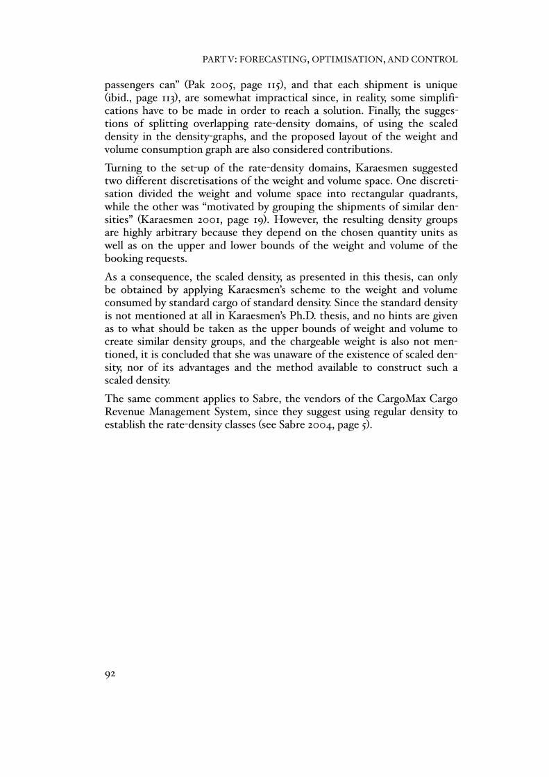
passengers can” (Pak 2005, page 115), and that each shipment is unique (ibid., page 113), are somewhat impractical since, in reality, some simplifi-cations have to be made in order to reach a solution. Finally, the sugges-tions of splitting overlapping rate-density domains, of using the scaled density in the density-graphs, and the proposed layout of the weight and volume consumption graph are also considered contributions.

Turning to the set-up of the rate-density domains, Karaesmen suggested two different discretisations of the weight and volume space. One discreti-sation divided the weight and volume space into rectangular quadrants, while the other was “motivated by grouping the shipments of similar den-sities” (Karaesmen 2001, page 19). However, the resulting density groups are highly arbitrary because they depend on the chosen quantity units as well as on the upper and lower bounds of the weight and volume of the booking requests.

As a consequence, the scaled density, as presented in this thesis, can only be obtained by applying Karaesmen’s scheme to the weight and volume consumed by standard cargo of standard density. Since the standard density is not mentioned at all in Karaesmen’s Ph.D. thesis, and no hints are given as to what should be taken as the upper bounds of weight and volume to create similar density groups, and the chargeable weight is also not men-tioned, it is concluded that she was unaware of the existence of scaled den-sity, nor of its advantages and the method available to construct such a scaled density.

The same comment applies to Sabre, the vendors of the CargoMax Cargo Revenue Management System, since they suggest using regular density to establish the rate-density classes (see Sabre 2004, page 5).


92

7 Flight Revenue Optimisation

The optimal flight revenue is the revenue which could be earned by filling the available capacity of a flight with the most profitable booking requests. The process of confirming the profitable booking requests and rejecting the unprofitable ones is, by its very nature, a series of either/or decisions that leads to an integer optimisation model with binary (0-1) decision vari-ables. In order to be able to run such a model some time before departure it is, of course, necessary to forecast the rate and the density of future booking requests, as well as their size. However, empirical evidence sug-gests that the size of future booking requests cannot reliably be forecast. Therefore, an alternative approach that may be more reliable is to forecast the aggregated demand of the domains, and to assume that this aggregated demand can be confirmed partly, even though Pak (2005, page 122) correct-ly states that “the cargo problem […] is a 0–1 decision problem for which the LP [Linear Programming]-relaxation is a very crude approximation.”

The next assumption concerns the stochastic nature of the demand. As de Boer et al. (1999) put it, “one should expect that ignoring the probabilistic nature of demand has a negative impact on total revenue” (page 4), and the example they gave to illustrate this point is remarkably simple (although it is from Passenger Revenue Management): “Suppose that the upper fare classes are highly more profitable. Then it would certainly be rewarding to reserve more high-fare seats than the airline actually expects to sell on average, in order to earn the upward potential of high-fare demand” (ibid., page 4).

Despite this, and even though it is explicitly accepted that the perfect fore-cast does not exist, the models which will be presented in this chapter do assume that there is no forecast error that has to be dealt with. This as-sumption is not as illogical as it first sounds because empirical evidence at a major European cargo airline using demand forecasts from various vendors of Cargo Revenue Management Systems has shown that it is not only difficult to come up with a good demand forecast, it is also very difficult to anticipate its likely error and, crucially, an inaccurate estimate of the error can make a bad forecast worse.

In the first two sections of this chapter, two linear programming models that can calculate expected flight revenue will be presented. The first model is referred to as the primal model to calculate flight revenue, and the second model is labelled the dual model. The Kuhn-Tucker Conditions for the models are discussed in the third section, and the preferred location of the rate-density domains within the rate-density grids are discussed in the fourth section. Finally, the contribution of this chapter is outlined in Section 5.

93

7.1 Primal Model to Calculate the Revenue of a Flight

The primal model is a linear program that is able to calculate the maximum revenue of a single flight (i.e., a single flight with a particular flight ID). A brief outline of the primal model’s indices and parameters is given below.

Indices:i0 rate-density domain index s0 flight segment indexl0 flight leg index

Parameters:bwcl0 [0, ∞) [chkg]0 0 bookable weight capacity of flight leg lbvcl0 [0, ∞) [chkg]0 0 bookable volume capacity of flight leg lqis0 [0, ∞) [chkg]0 0 demand-to-come of rate-density domain i 0 0 0 0 of flight segment sris0 [0, ∞) [€/chkg]0 rate of rate-density domain i 0 0 0 0 of flight segment swis0 [0, 1] [chkg/chkg]0 weight coefficient of rate-density domain i 0 0 0 0 of flight segment svis0 [0, 1] [chkg/chkg]0 volume coefficient of rate-density domain i 0 0 0 0 of flight segment sals0 {0, 1} [unitless]0 incidence coefficient of flight leg l 0 0 0 0 on flight segment s

The above indices and parameters have already been discussed, so only the new decision and slack variables of the primal model need to be explained.

Primal Decision and Slack Variables:xis0 [0, ∞) [chkg]0 0 selected demand of rate-density domain i 0 0 0 0 of flight segment ssis0 [0, ∞) [chkg]0 0 demand slack of rate-density domain i 0 0 0 0 of flight segment sfwcl0 [0, ∞) [chkg]0 0 free weight capacity of flight leg lfvcl0 [0, ∞) [chkg]0 0 free volume capacity of flight leg l

The primal decision variable xis denotes how much of the demand for the rate-density domain i of flight segment s should be confirmed, the primal slack variable sis denotes how much of the demand for rate-density domain i of flight segment s should be rejected, and the primal slack variables fwcl and fvcl denote how much weight and volume capacity is expected to be free on flight leg l. Note that all the primal variables are subjected to a non-negativity constraint to reflect the reality of the situation.

The flight revenue variable is introduced below. This is the objective varia-ble of the primal model and is, given its value range, a free variable.

Primal Objective Variable:fr 0 [– ∞, ∞] [€]0 0 flight revenue

A graphical illustration of some of the primal parameters and variables is given in Figure 28. Since the figure is an illustration of primal quantities, it is mainly focused on supply and demand.


94

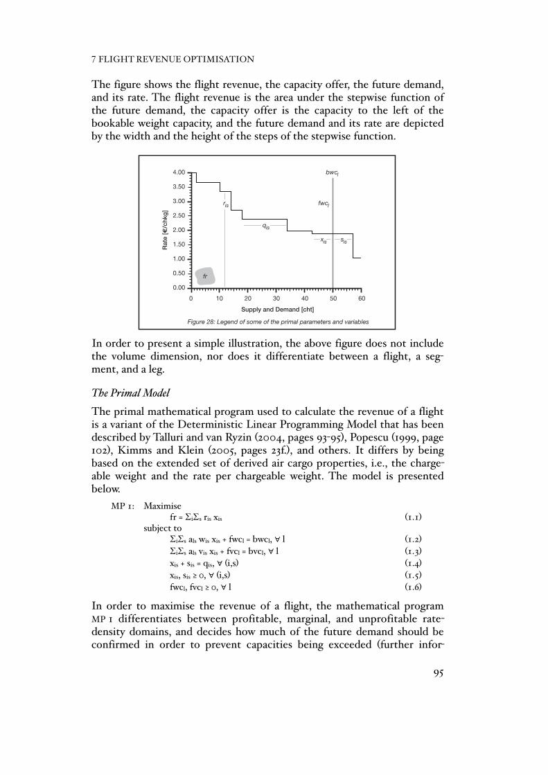
The figure shows the flight revenue, the capacity offer, the future demand, and its rate. The flight revenue is the area under the stepwise function of the future demand, the capacity offer is the capacity to the left of the bookable weight capacity, and the future demand and its rate are depicted by the width and the height of the steps of the stepwise function.

In order to present a simple illustration, the above figure does not include the volume dimension, nor does it differentiate between a flight, a seg-ment, and a leg.

The Primal Model

The primal mathematical program used to calculate the revenue of a flight is a variant of the Deterministic Linear Programming Model that has been described by Talluri and van Ryzin (2004, pages 93-95), Popescu (1999, page 102), Kimms and Klein (2005, pages 23f.), and others. It differs by being based on the extended set of derived air cargo properties, i.e., the charge-able weight and the rate per chargeable weight. The model is presented below.

MP 1:0 Maximise0 0 fr = ∑i∑s ris xis0 0 0 0 0 0 0 (1.1)0 subject to0 0 ∑i∑s als wis xis + fwcl = bwcl, ∀ l0 0 0 0 0 (1.2)0 0 ∑i∑s als vis xis + fvcl = bvcl, ∀ l0 0 0 0 0 (1.3)0 0 xis + sis = qis, ∀ (i,s)0 0 0 0 0 0 0 (1.4)0 0 xis, sis ≥ 0, ∀ (i,s)0 0 0 0 0 0 0 (1.5)0 0 fwcl, fvcl ≥ 0, ∀ l 0 0 0 0 0 0 0 (1.6)

In order to maximise the revenue of a flight, the mathematical program MP 1 differentiates between profitable, marginal, and unprofitable rate-density domains, and decides how much of the future demand should be confirmed in order to prevent capacities being exceeded (further infor-

mpsmwps mvps

XX

Varia

ble

density[mc/t]

(revenue)[€]

revenue[€]

revenue[€]

rate[€/kg]

weight[kg]

(volume)[mc]

weight[kg]

weight[kg]

volume[mc]

density[mc/kg]

weight[kg]

–> derivedinitial


Properties


0 1/12 1/6 1/4 1/3 5/12 1/2


Cha

rgea

ble

Wei

ght [

chkg

]

1.0

0.8

0.6

0.4

0.2

0

6

CD

0 1 32 54

void

void

Density [mc/t]

BCAB

CD'

BC'

AB'

volume c

onsumptio

n

weight consumption



Cha

rgea

ble

Wei

ght [

chkg

]

1.0

0.8

0.6

0.4

0.2

0

6

void

void

Density [mc/t]

7 98 1110 12

FGEFDE

FG'EF'

DE'

0.5 0.75

weight consumption

volume consumption

8/117/106/95/84/7


0 10 20 30 40 6050

4.00

3.50

3.00

2.50

2.00

0.50

1.50

1.00

0.00


Rat

e [€

/chk

g]

qis

ris fwcl

sisxis

fr


0 10 20 30 40 6050

4.00

3.50

3.00

2.50

2.00

0.50

1.50

1.00

0.00


Rat

e an

d C

ost [

€/c

hkg]

qis

ris

pis

uis

mwpl

fr

bwclbwcl

mps

2 4 96 18

Rat

e [€

/chk

g]


Density [mc/t]

9r

8r

7r

6r

5r

4r

3r

2r

1 0 = r

0 !

mwps

mvps

fps

fvps




10 = cw

2cw

3cw

4cw

5cw

6cw

cwharg

eabl

e W

eigh

t [ch

t]

bcsbwcs

mps

Rat

e [€

/chk

g]

9r

8r

7r

6r

5r

4r

3r

2r

1 0 = r

mwps

mvps

fp

a

a

s

fvps


profitable

not profitable

feasible

rActual Booking

Request


q10 = cw

2cw

3cw

4cw

5cw

6cw

cwharg

eabl

e W

eigh

t [ch

t]

bcsbwcs

Rat

e [€

/chk

g]

9r

8r

7r

6r

5r

4r

3r

2r

1 0 = r

fps

fvps


profitable

feasible

fcsfvcs

fwcs

definitely feasible



fvcsfwcs fcs

s

a

ar

q

7 FLIGHT REVENUE OPTIMISATION

95

mation about profitable, marginal, and unprofitable domains can be found in Section 3 of this chapter). More specifically, the decision variables xis act as selectors for the demand. If the bookable capacities of a particular leg are higher than the capacity consumption of the selected demand, the ca-pacities are sufficient and the corresponding slack variables take a positive value. These slack variables are either the ‘free weight capacity’ of a leg (i.e., fwcl) or its ‘free volume capacity’ (i.e., fvcl). Another slack variable is the ‘demand slack’. If the selected demand of a particular rate-density domain is less than the expected demand, the corresponding demand slack (i.e., sis) will take a positive value.

Maximising flight revenue is subjected to several constraints: the weight constraints (1.2) require that the weight of the selected future demand is less than or equal to the bookable weight capacity, the volume constraints (1.3) require the volume of the selected future demand to be less than or equal to the bookable volume capacity, and the demand constraints (1.4) require the selected demand to be lower than or equal to the expected future demand. Finally, non-negativity constraints are imposed on all the variables; see (1.5) and (1.6).

In contrast to the decision variables and the slack variables, the revenue variable in (1.1) is not subjected to a non-negativity constraint because, as a rule, the objective variable in a linear program is left unrestricted (although the flight revenue will not be negative given the nature of revenue maximi-sation).

A technical aside is that, in a professional implementation, the primal slack variables would be rendered superfluous by using ≤ constraints as well as simple upper bounds. The reason for including the slack variables in the mathematical program MP 1 is that this avoids having to define them sepa-rately.

The major benefit of the presented quantity-based primal model to calcu-late the revenue of a flight is that all the variables and right-hand sides (except the objective variable) share the same quantity unit. The free weight and volume capacities, for example, can be easily compared with demand slack because they are all expressed in chargeable kilograms.

In order to prepare for the subsequent situation where the free capacities are needed on a segment level, free segment capacities are defined below.

The Free Segment Capacities

Free segment weight and volume capacities are calculated on the basis of the free leg weight and volume capacities, and denote how much weight and volume are expected to be free on each segment at the time of the segment’s departure.


96

The free segment capacities play an important role later in the booking request control since they indicate how large an actual booking request can be in order for it to be confirmed irrespective of its rate.

Free Segment Weight and Volume Capacities:fwcs0 [0, ∞) [chkg]0 0 free weight capacity of flight segment sfvcs0 [0, ∞) [chkg]0 0 free volume capacity of flight segment s

The units for the free segment weight and volume capacities are chargeable kilograms, and the value ranges of both are brought forward from the value ranges of the free leg weight and volume capacities.

The free weight and volume capacities of a segment are defined as the min-imum values of the included free leg weight and volume capacities. Hence, the free weight and volume capacities of a segment are determined by its bottlenecks. A more formal definition is given below.

Free Segment Weight and Volume Capacities as a Function of Free Leg Weight and Volume Capacities:fwcs = min {fwcl, ∀ l where als = 1}fvcs = min {fvcl, ∀ l where als = 1}

Free segment capacity is considered next. The free segment capacity de-notes how much chargeable weight, of a given density, is expected to be free on a particular segment at the time of the segment’s departure. The free segment capacity should not be confused with the free segment weight capacity or the free segment volume capacity.

Free Segment Capacity:fcs0 [0, ∞) [chkg]0 0 free capacity of flight segment s

The unit of the free segment capacity is again the chargeable kilogram, and its value range is the same as the value range of the free segment weight capacity and the free segment volume capacity (i.e., any non-negative value). The definition of the free segment capacity, as a function of the unified density, is given below.

Free Segment Capacity as a Function of Unified Density:if0 0 < fwcs ≤ fvcs 0 and 0 ≤ ud ≤ 0.50 0 0 then fcs = fwcs elseif0 (as above) 0 0 and 0.5 < ud ≤ 0.5 (fvcs/fwcs)0 then fcs = fwcs/(2 – 2ud)elseif0 (as above) 0 0 and 0.5 (fvcs/fwcs) < ud ≤ 10 0 then fcs = fvcs elseif0 0 = fwcs ≤ fvcs 0 and 0 ≤ ud < 10 0 0 then fcs = 0elseif0 (as above)0 0 and ud = 10 0 0 0 then fcs = fvcs elseif0 0 < fvcs < fwcs 0 and 0 ≤ ud ≤ 0.5 (fvcs/fwcs)0 0 then fcs = fwcs

elseif0 (as above) 0 0 and 0.5 (fvcs/fwcs) < ud ≤ 0.50 then fcs = fvcs/2udelseif0 (as above) 0 0 and 0.5 < ud ≤ 10 0 0 then fcs = fvcs elseif0 0 = fvcs < fwcs 0 and 0 < ud ≤ 10 0 0 then fcs = 0elseif0 (as above)0 0 and ud = 00 0 0 0 then fcs = fwcs elseif0 0 = fwcs = fvcs 0 and 0 ≤ ud ≤ 10 0 0 then fcs = 0


97

The free segment capacities can be visualised with the help of free segment capacity graphs. A free segment capacity graph shows the free segment ca-pacity as a function of its scaled density. Free segment capacity graphs are considered primal graphs since they visualise the free capacities of the pri-mal model MP 1.

In general, a free segment capacity graph displays three different capacities: the free segment weight capacity, the free segment volume capacity, and the free segment capacity. The free segment weight capacity is shown at the density value of zero, the free segment volume capacity is shown at the density value of infinity, and the free segment capacity is the vertical dis-tance between the top of the graph and the free segment capacity curve. For reasons which will become clear later, the zero reference line for the free capacities is located at the top of the graph.

Two example graphs are shown below. The first graph (Figure 29) shows the free segment capacity for various amounts of free segment volume capacity, whereas the second graph (Figure 30) shows the free segment capacity for various amounts of free segment weight capacity. Neither of these paramet-ric variations is considered part of the actual free segment capacity graph, but they do illustrate the behaviour of the free segment capacity curve.

The free segment weight capacity fwcs in Figure 29 is assumed to be equal to cw3, the free segment volume capacity fvcs is assumed to be equal to cw2, and the free segment capacity is the connecting curve shown in black. The grey curves, in comparison, show the effect of a parametric increase in the free segment volume capacity.

The graph on the next page (Figure 30) shows the effect of a parametric increase in the free segment weight capacity (as opposed to the volume ca-pacity increase illustrated above).

10 = cw

2cw

3cw

4cw

5cw

6cw

7cw

8cw

9 cw

00

XI

2 4 96 !18

Density [mc/t]

Cha

rgea

ble

Wei

ght [

cht]

A primal graph with various bookable volume capacities

Stowage loss limiting factors and the economic properties of a booking request

Limiting Factor

Eco

nom

ic P

rope

rty

booking request profitabilityflight volume capacity

D sl

r sl

d sl

—yes

—yes

yes—

—yes

—no

yes—

0 " max " vc/wcvc/wc < max " !d sl

d sl


d sl


d sl


d sl


d sl


d sl

The favorability of a stowage loss and of changing the economic properties

Density Rank

Eco

nom

ic P

rope

rty

D sl

r sl

unfavorableunfavorableneutral

unfavorable

unfavorable unfavorableunfavorable

unfavorableneutral

favorableunfavorable,

neutral orfavorable

unfavorabled sl

d " vc/wc " max d sl vc/wc < d " max d sld " max < vc/wcd sl

stowage lossstowage loss yes0 " max " !d slyes0 " max " !d sl

segment j

2 4 96 !18

Density [mc/t]

Cha

rgea

ble

Wei

ght [

cht]

A primal graph with various bookable weight capacities

segment j

10 = cw

2cw

3cw

4cw

5cw

6cw

7cw

8cw

9 cw

0

fc j

10 = cw

bcj

fcj fvcj

fwcj

bwcjbvcj

bcj

fvcj

fwcj

bwcj

bvcj

2 4 96 !18

Density [mc/t]

Cha

rgea

ble

Wei

ght [

cht]

Figure 30: Primal graph with various free weight capacities

10 = cw

2cw

3cw

4cw

5cw

6cw

7cw

8cw

9 cw

0

fcs fvcs

fwcs

10 = cw

2cw

3cw

4cw

5cw

6cw

7cw

8cw

9 cw

00 2 4 96 !18

Density [mc/t]

Cha

rgea

ble

Wei

ght [

cht]

Figure 29: Primal graph with various free volume capacities

fcsfvcs

fwcs

0 2 4 96 !18

4.00

3.50

3.00

2.50

2.00

0.50

1.50

1.00

0.00

Density [mc/t]

Rat

e [€

/chk

g]

Figure 34: Rate-density domains, gravity centres, and the marginal segment price

i=1 2

31 32

25 3029282726

21 242322

15 2019181716

9 1413121110

3 87654

10 = cw

2cw

3cw

4cw

5cw

6cw

7cw

8cw

9 cw

00 2 4 96 !18

Density [mc/t]

Cha

rgea

ble

Wei

ght [

cht]

Figure 35: Free and bookable segment capacities, and the primal modes

fcs

bcs

fvcs

fwcs

bwcs

bvcs

definitely feasible(primal mode 1)

feasible(primal mode 2)

not feasible(primal mode 3)

s

ss

s


98

The free segment weight capacity fwcs in Figure 30 is assumed to be equal to cw3, the free segment volume capacity fvcs is assumed to be equal to cw2, and the resulting free segment capacity is the connecting curve shown in black. The grey curves, in comparison, show the effect of an increase in weight capacity.

7.2 Dual Model to Calculate the Revenue of a Flight

The dual model is a price-based linear program that is, like the primal model, able to calculate the optimal revenue of a single flight. The advan-tage is that it also calculates the marginal prices of the weight and volume capacities. The indices and parameters used in the dual model are the same as in the primal model, and so only the decision and slack variables of the dual model need to be defined here.

Dual Decision and Slack Variables:mwpl0 [0, ∞] [€/chkg]0 marginal price of weight capacity of flight leg lmvpl0 [0, ∞] [€/chkg]0 marginal price of volume capacity of flight leg lpis0 [0, ∞) [€/chkg]0 profitability of rate-density domain i 0 0 0 0 of flight segment suis0 [0, ∞) [€/chkg]0 unprofitability of rate-density domain i 0 0 0 0 of flight segment s

The dual decision variables mwpl and mvpl denote the marginal prices of the bookable weight and volume capacities on flight leg l, the dual decision variable pis denotes the profitability of rate-density domain i of flight seg-ment s, and the dual slack variable uis denotes the unprofitability of rate-density domain i of flight segment s (further information on profitable and unprofitable domains can be found in Section 3 of this chapter). All the dual variables are subjected to non-negativity constraints to reflect their re-stricted value range.

10 = cw

2cw

3cw

4cw

5cw

6cw

7cw

8cw

9 cw

00

XI

2 4 96 !18

Density [mc/t]

Cha

rgea

ble

Wei

ght [

cht]



Limiting Factor

Eco

nom

ic P

rope

rty


D sl

r sl

d sl

—yes

—yes

yes—

—yes

—no

yes—


d sl


d sl


d sl


d sl


d sl


d sl


Density Rank

Eco

nom

ic P

rope

rty

D sl

r sl


unfavorable


unfavorableneutral


neutral orfavorable

unfavorabled sl



segment j

2 4 96 !18

Density [mc/t]

Cha

rgea

ble

Wei

ght [

cht]


segment j

10 = cw

2cw

3cw

4cw

5cw

6cw

7cw

8cw

9 cw

0

fc j

10 = cw

bcj

fcj fvcj

fwcj

bwcjbvcj

bcj

fvcj

fwcj

bwcj

bvcj

2 4 96 !18

Density [mc/t]

Cha

rgea

ble

Wei

ght [

cht]


10 = cw

2cw

3cw

4cw

5cw

6cw

7cw

8cw

9 cw

0

fcs fvcs

fwcs

10 = cw

2cw

3cw

4cw

5cw

6cw

7cw

8cw

9 cw

00 2 4 96 !18

Density [mc/t]

Cha

rgea

ble

Wei

ght [

cht]


fcsfvcs

fwcs

0 2 4 96 !18

4.00

3.50

3.00

2.50

2.00

0.50

1.50

1.00

0.00

Density [mc/t]

Rat

e [€

/chk

g]


i=1 2

31 32

25 3029282726

21 242322

15 2019181716

9 1413121110

3 87654

10 = cw

2cw

3cw

4cw

5cw

6cw

7cw

8cw

9 cw

00 2 4 96 !18

Density [mc/t]

Cha

rgea

ble

Wei

ght [

cht]


fcs

bcs

fvcs

fwcs

bwcs

bvcs




s

ss

s


99

The objective variable is again the flight revenue. The flight revenue of the dual model is, as was the case in the primal model, a free variable.

Dual Objective Variable:fr 0 [– ∞, ∞] [€]0 0 flight revenue

A graphical illustration showing some of the dual parameters and variables is given in Figure 31. Since the figure is an illustration of dual prices, it is fo-cussed on rate and cost. Although this figure is very similar to Figure 28, it is worth noting that the figure below takes a ‘dual point of view’ while the earlier figure took a ‘primal point of view’.

The above figure shows the flight revenue, the capacity price, and the fu-ture demand and its rate. The flight revenue is the area under the stepwise function of the future demand, the capacity price is the price used to value the bookable weight capacity, and the future demand and its rate are depicted by the width and the height of the steps of the stepwise function.

It can be observed that the above figure does not include the volume di-mension. In order to produce a simple representation of the subject, the figure also does not differentiate between a flight, a segment, and a leg.

The Dual Model

The dual mathematical program to calculate the revenue of a flight is the dual of the previously presented primal model.

MP 2:0 Minimise0 0 fr = ∑l bwcl mwpl + ∑l bvcl mvpl + ∑i∑s qis pis0 0 0 (2.1)0 subject to0 0 ∑l als wis mwpl + ∑l als vis mvpl + pis – uis = ris, ∀ (i,s)0 0 (2.2)0 0 pis, uis ≥ 0, ∀ (i,s)0 0 0 0 0 0 0 (2.3)0 0 mwpl, mvpl ≥ 0, ∀ l0 0 0 0 0 0 0 (2.4)

mpsmwps mvps

XX

Varia

ble

density[mc/t]

(revenue)[€]

revenue[€]

revenue[€]

rate[€/kg]

weight[kg]

(volume)[mc]

weight[kg]

weight[kg]

volume[mc]

density[mc/kg]

weight[kg]

–> derivedinitial


Properties


0 1/12 1/6 1/4 1/3 5/12 1/2


Cha

rgea

ble

Wei

ght [

chkg

]

1.0

0.8

0.6

0.4

0.2

0

6

CD

0 1 32 54

void

void

Density [mc/t]

BCAB

CD'

BC'

AB'

volume c

onsumptio

n

weight consumption



Cha

rgea

ble

Wei

ght [

chkg

]

1.0

0.8

0.6

0.4

0.2

0

6

void

void

Density [mc/t]

7 98 1110 12

FGEFDE

FG'EF'

DE'

0.5 0.75

weight consumption

volume consumption

8/117/106/95/84/7


0 10 20 30 40 6050

4.00

3.50

3.00

2.50

2.00

0.50

1.50

1.00

0.00


Rat

e [€

/chk

g]

qis

ris fwcl

sisxis

fr


0 10 20 30 40 6050

4.00

3.50

3.00

2.50

2.00

0.50

1.50

1.00

0.00


Rat

e an

d C

ost [

€/c

hkg]

qis

ris

pis

uis

mwpl

fr

bwclbwcl

mps

2 4 96 18R

ate

[€/c

hkg]


Density [mc/t]

9r

8r

7r

6r

5r

4r

3r

2r

1 0 = r

0 !

mwps

mvps

fps

fvps




10 = cw

2cw

3cw

4cw

5cw

6cw

cwharg

eabl

e W

eigh

t [ch

t]

bcsbwcs

mps

Rat

e [€

/chk

g]

9r

8r

7r

6r

5r

4r

3r

2r

1 0 = r

mwps

mvps

fp

a

a

s

fvps


profitable

not profitable

feasible

rActual Booking

Request


q10 = cw

2cw

3cw

4cw

5cw

6cw

cwharg

eabl

e W

eigh

t [ch

t]

bcsbwcs

Rat

e [€

/chk

g]

9r

8r

7r

6r

5r

4r

3r

2r

1 0 = r

fps

fvps


profitable

feasible

fcsfvcs

fwcs

definitely feasible



fvcsfwcs fcs

s

a

ar

q


100

In order to minimise the revenue of a flight, mathematical program MP 2 distinguishes between sufficient and insufficient leg weight and volume capacities, and decides how much of the rate must be assigned to the insuf-ficient capacities in order to prevent the unprofitable demand from being confirmed (further information about sufficient and insufficient capacities can be found in Section 3 of this chapter). More specifically, the decision variables mwpl and mvpl act as prices for the weight and volume capacities. If the rate of a particular rate-density domain is too low to cover the costs of its capacity utilisation, the domain is unprofitable and the corresponding slack variable ‘unprofitability’ uis takes a positive value. Conversely, if the rate is higher than the value needed for the demand to be confirmed, the domain is profitable and the ‘profitability’ variable pis takes a positive value. Finally, if the rate of a particular rate-density domain exactly matches the costs of the capacity utilisation, the domain is neither profitable nor un-profitable but marginal, with both uis and pis being equal to zero.

The minimisation of flight revenue is subjected to several constraints: the profitability constraints (2.2) require that the value of a rate-density do-main’s weight consumption plus the value of its volume consumption plus the profit of the domain is higher than or equal to its rate. Furthermore, non-negativity constraints are imposed on all the variables; see (2.3) and (2.4).

Again, it is convenient for the revenue variable in (2.1) to be a free variable because, this time, the flight revenue has to serve as the objective value of the dual mathematical program.

As was the case with the primal constraints, the format of the dual con-straints is not the ideal option. In a professional implementation, the dual slack variables would have been rendered superfluous by using ≥ con-straints.

The major benefit of the presented price-based dual model is that, once again, all the variables and right-hand sides (except the objective variable) share the same quantity unit. The marginal weight and volume prices, for example, can be easily compared with a domain rate because all of them are expressed in euro per chargeable kilogram.

In order to prepare for the subsequent situation where the marginal prices are needed on a segment level, the marginal segment prices are introduced next.


101

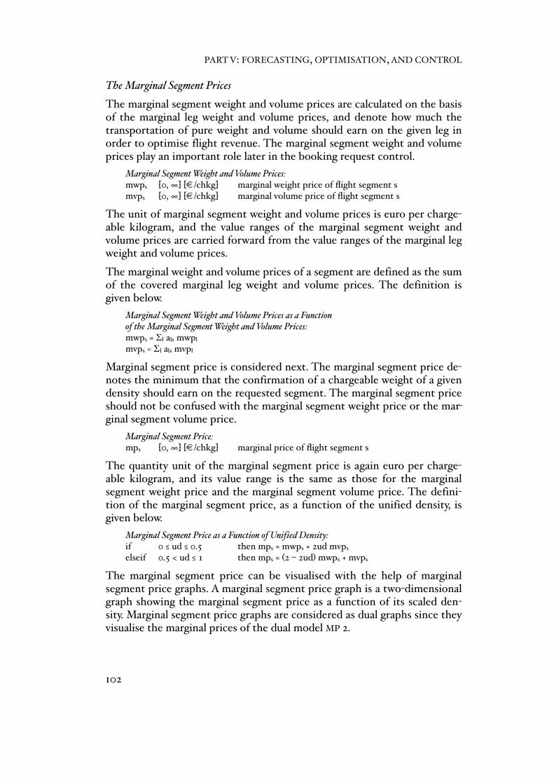
The Marginal Segment Prices

The marginal segment weight and volume prices are calculated on the basis of the marginal leg weight and volume prices, and denote how much the transportation of pure weight and volume should earn on the given leg in order to optimise flight revenue. The marginal segment weight and volume prices play an important role later in the booking request control.

Marginal Segment Weight and Volume Prices:mwps0 [0, ∞] [€/chkg]0 marginal weight price of flight segment smvps0 [0, ∞] [€/chkg]0 marginal volume price of flight segment s

The unit of marginal segment weight and volume prices is euro per charge-able kilogram, and the value ranges of the marginal segment weight and volume prices are carried forward from the value ranges of the marginal leg weight and volume prices.

The marginal weight and volume prices of a segment are defined as the sum of the covered marginal leg weight and volume prices. The definition is given below.

Marginal Segment Weight and Volume Prices as a Function of the Marginal Segment Weight and Volume Prices:mwps = ∑l als mwpl

mvps = ∑l als mvpl

Marginal segment price is considered next. The marginal segment price de-notes the minimum that the confirmation of a chargeable weight of a given density should earn on the requested segment. The marginal segment price should not be confused with the marginal segment weight price or the mar-ginal segment volume price.

Marginal Segment Price:mps0 [0, ∞] [€/chkg]0 marginal price of flight segment s

The quantity unit of the marginal segment price is again euro per charge-able kilogram, and its value range is the same as those for the marginal segment weight price and the marginal segment volume price. The defini-tion of the marginal segment price, as a function of the unified density, is given below.

Marginal Segment Price as a Function of Unified Density:if0 0 ≤ ud ≤ 0.50 0 then mps = mwps + 2ud mvps

elseif0 0.5 < ud ≤ 10 0 then mps = (2 – 2ud) mwps + mvps

The marginal segment price can be visualised with the help of marginal segment price graphs. A marginal segment price graph is a two-dimensional graph showing the marginal segment price as a function of its scaled den-sity. Marginal segment price graphs are considered as dual graphs since they visualise the marginal prices of the dual model MP 2.


102

In general, a marginal segment price graph displays three different prices: the marginal segment weight price, the marginal segment volume price and the marginal segment price. The marginal segment weight price is shown at the density value of zero, the marginal segment volume price is shown at the density value of infinity, and the marginal segment price is the vertical distance between the bottom of the graph (i.e., the x-axis) and the marginal segment price curve.

Two example graphs are included (Figures 32 and 33). The first shows the marginal segment price for various levels of marginal segment volume price, and the second shows the marginal segment price for various marginal segment weight prices. Neither of these parametric variations is considered part of the actual marginal segment price graph, but they do illustrate the behaviour of the marginal segment price curve.

The marginal segment weight price, mwps, in Figure 32 is assumed to be equal to r2, the marginal segment volume price mvps is assumed to be equal to r3, and the marginal segment price is the connecting line shown in black. The grey curves, in comparison, show the effect of a parametric increase in the marginal segment volume price.

The following graph shows the effect of a parametric increase in the mar-ginal segment weight price (as opposed to the volume price increase that was illustrated above).

The marginal segment weight price, mwps, in Figure 33 (see Page 104) is as-sumed to be equal to r1 (i.e., zero), the marginal segment volume price, mvps, is assumed to be equal to r3, and the resulting marginal segment price is the connecting line in black. The grey curves, in comparison, show the effect of an increase in volume price.

segment j

forecastdomain i

456

[chkg]

123

789

…

……

……

D22

0 2 4 96 18

8.00

7.00

6.00

5.00

4.00

1.00

3.00

2.00

0.00


Rat

e [e

uro/

chkg

]


!

……

…

…

…

…

…

…

…

…

…

…

…

…

…

…

…

…

…

…

…

…

…

…

… …

…

…

…

…

D27

… …

…

…

1000

12001750

…

Di [chkg]

X

mpj

2 4 96 18

Rat

e [e

uro/

chkg

]

2 4 96 !18

Rat

e [e

uro/

chkg

]




……

……

Density [mc/t]

Rat

e [e

uro/

chkg

]


……

…

…

…

…

…

…

…

…

…

…

…

…

…

…

…

…

…

…

…

… …

…

…

…

…

… …

…

…

…

9r

8r

7r

6r

5r

4r

3r

2r

1r

D21

1500

DijD7j

D2jD1j

123

[chkg]456

…

……

Density [mc/t]

Rat

e [€

/chk

g]


……

…

…

…

…

…

…

…

…

…

…

…

…

…

…

…

…

…

…

…… … …

…

… …

…

…

…

…

… …

… … …

…

9r

8r

7r

6r

5r

4r

3r

2r

7d6d5d4d3d2d1d1r

qis

s

s

s

123

789

[chkg]

456

……

……

Density [mc/t]

Rat

e [e

uro/

chkg

]


……

…

…

…

…

…

…

…

…

…

…

…

…

…

…

…

…

…

…

…

… …

…

…

…

…

… …

…

…

…

9r

8r

7r

6r

5r

4r

3r

2r

1r

DijD7j

D2jD1j

4847

42

0 2 4 96 18 !

Density [mc/t]

Density [mc/t]

segment j

9r

8r

7r

6r

5r

4r

3r

2r

1 0 = r

0

9r

8r

7r

6r

5r

4r

3r

2r

1 0 = r

0

!

segment j

i=1 6543

7 …

2

… ……

……

2 4 96 18

Rat

e [€

/chk

g]


Density [mc/t]

9r

8r

7r

6r

5r

4r

3r

2r

1 0 = r

0 !

mwpsmvps

mps

2 4 96 !18

Rat

e [€

/chk

g]


Density [mc/t]

9r

8r

7r

6r

5r

4r

3r

2r

1 0 = r

0

mwps

mvpsmps

mwpj

mvpj

lwpjlvpj

lpj

lwpj

lvpj

lpj

mwpj

mvpj

mpj


103

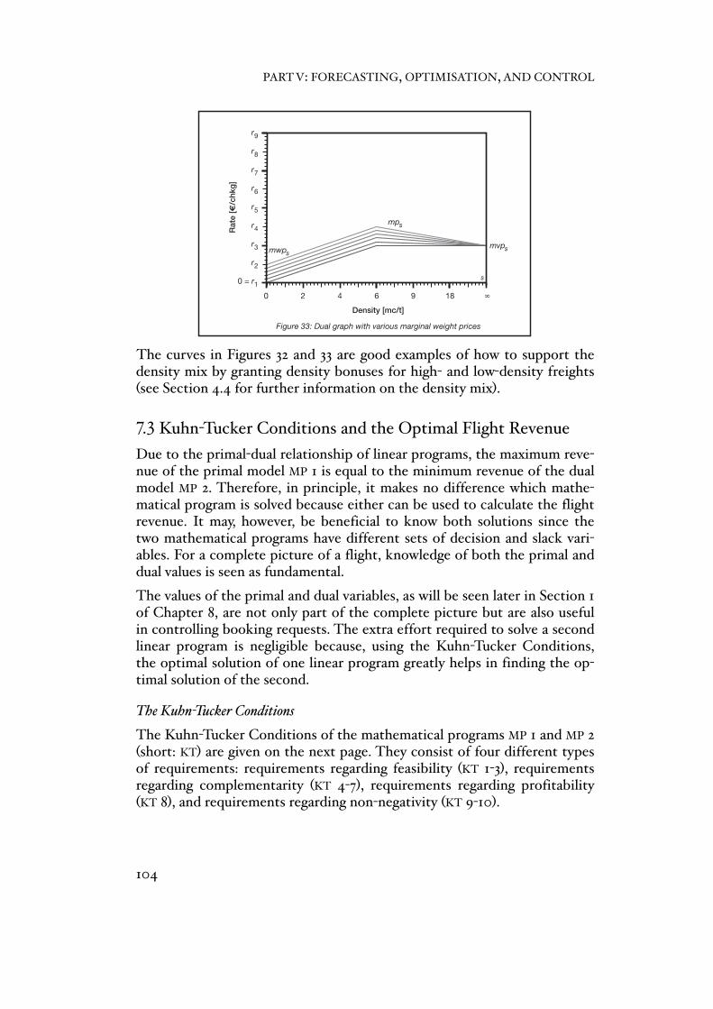
The curves in Figures 32 and 33 are good examples of how to support the density mix by granting density bonuses for high- and low-density freights (see Section 4.4 for further information on the density mix).

7.3 Kuhn-Tucker Conditions and the Optimal Flight Revenue

Due to the primal-dual relationship of linear programs, the maximum reve-nue of the primal model MP 1 is equal to the minimum revenue of the dual model MP 2. Therefore, in principle, it makes no difference which mathe-matical program is solved because either can be used to calculate the flight revenue. It may, however, be beneficial to know both solutions since the two mathematical programs have different sets of decision and slack vari-ables. For a complete picture of a flight, knowledge of both the primal and dual values is seen as fundamental.

The values of the primal and dual variables, as will be seen later in Section 1 of Chapter 8, are not only part of the complete picture but are also useful in controlling booking requests. The extra effort required to solve a second linear program is negligible because, using the Kuhn-Tucker Conditions, the optimal solution of one linear program greatly helps in finding the op-timal solution of the second.

The Kuhn-Tucker Conditions

The Kuhn-Tucker Conditions of the mathematical programs MP 1 and MP 2 (short: KT) are given on the next page. They consist of four different types of requirements: requirements regarding feasibility (KT 1-3), requirements regarding complementarity (KT 4-7), requirements regarding profitability (KT 8), and requirements regarding non-negativity (KT 9-10).

segment j

forecastdomain i

456

[chkg]

123

789

…

……

……

D22

0 2 4 96 18

8.00

7.00

6.00

5.00

4.00

1.00

3.00

2.00

0.00


Rat

e [e

uro/

chkg

]


!

……

…

…

…

…

…

…

…

…

…

…

…

…

…

…

…

…

…

…

…

…

…

…

… …

…

…

…

…

D27

… …

…

…

1000

12001750

…

Di [chkg]

X

mpj

2 4 96 18

Rat

e [e

uro/

chkg

]

2 4 96 !18

Rat

e [e

uro/

chkg

]




……

……

Density [mc/t]

Rat

e [e

uro/

chkg

]


……

…

…

…

…

…

…

…

…

…

…

…

…

…

…

…

…

…

…

…

… …

…

…

…

…

… …

…

…

…

9r

8r

7r

6r

5r

4r

3r

2r

1r

D21

1500

DijD7j

D2jD1j

123

[chkg]456

…

……

Density [mc/t]

Rat

e [€

/chk

g]


……

…

…

…

…

…

…

…

…

…

…

…

…

…

…

…

…

…

…

…… … …

…

… …

…

…

…

…

… …

… … …

…

9r

8r

7r

6r

5r

4r

3r

2r

7d6d5d4d3d2d1d1r

qis

s

s

s

123

789

[chkg]

456

……

……

Density [mc/t]

Rat

e [e

uro/

chkg

]


……

…

…

…

…

…

…

…

…

…

…

…

…

…

…

…

…

…

…

…

… …

…

…

…

…

… …

…

…

…

9r

8r

7r

6r

5r

4r

3r

2r

1r

DijD7j

D2jD1j

4847

42

0 2 4 96 18 !

Density [mc/t]

Density [mc/t]

segment j

9r

8r

7r

6r

5r

4r

3r

2r

1 0 = r

0

9r

8r

7r

6r

5r

4r

3r

2r

1 0 = r

0

!

segment j

i=1 6543

7 …

2

… ……

……

2 4 96 18

Rat

e [€

/chk

g]


Density [mc/t]

9r

8r

7r

6r

5r

4r

3r

2r

1 0 = r

0 !

mwpsmvps

mps

2 4 96 !18

Rat

e [€

/chk

g]


Density [mc/t]

9r

8r

7r

6r

5r

4r

3r

2r

1 0 = r

0

mwps

mvpsmps

mwpj

mvpj

lwpjlvpj

lpj

lwpj

lvpj

lpj

mwpj

mvpj

mpj


104

Feasibility:0 ∑i∑s als wis xis + fwcl = bwcl, ∀ l0 0 0 0 0 0 (KT 1)0 ∑i∑s als vis xis + fvcl = bvcl, ∀ l0 0 0 0 0 0 (KT 2)

0 xis + sis = qis, ∀ (i,s)0 0 0 0 0 0 0 0 (KT 3)

Complementarity:0 mwpl fwcl = 0, ∀ l0 0 0 0 0 0 0 0 (KT 4)0 mvpl fvcl = 0, ∀ l0 0 0 0 0 0 0 0 (KT 5)0 pis sis = 0, ∀ (i,s)0 0 0 0 0 0 0 0 (KT 6)0 uis xis = 0, ∀ (i,s)0 0 0 0 0 0 0 0 (KT 7)

Profitability:0 ∑l als wis mwpl + ∑l als vis mvpl + pis – uis = ris, ∀ (i,s)0 0 0 (KT 8)

Non-Negativity:0 xis, sis, pis, uis ≥ 0, ∀ (i,s)0 0 0 0 0 0 0 (KT 9)0 fwcl, fvcl, mwpl, mvpl ≥ 0, ∀ l0 0 0 0 0 0 (KT 10)

The requirements regarding feasibility derive from the primal model MP 1, the requirements regarding complementarity replace the objective func-tions of MP 1 and MP 2, the requirements regarding profitability come from the dual model MP 2, and the requirements regarding non-negativity come from both models. The requirements regarding complementarity are also known as complementary slackness conditions.

The Complementary Slackness Conditions

The complementary slackness conditions link the decision variables of the primal model with the slack variables of the dual model, and the decision variables of the dual model with the slack variables of the primal model. More specifically, KT 4 and KT 5 emphasise the relationship between the marginal weight and volume prices of a leg and its free weight and volume capacities, while KT 6 and KT 7 specify the relationship between the profit-ability of a rate-density domain and its demand slack, as well as the rela-tionship between the unprofitability of a rate-density domain and its se-lected demand.

The relationship between the marginal weight and volume prices of a leg and its free weight and volume capacities can be applied at the segment level by reformulating the first pair of complementary slackness conditions so that they are valid for segments.

In other words, the complementary slackness condition mwpl fwcl = 0, ∀ l can be reformulated as mwps fwcs = 0, ∀ s, while the complementary slack-ness condition mvpl fvcl = 0, ∀ l can be reformulated as mvps fvcs = 0, ∀ s.


105

An economic interpretation of the reformulated conditions is given below:

❖ If a particular flight segment is expected to have a positive marginal weight price, the free weight capacity of that segment is zero.

❖ If a particular flight segment is expected to have a positive free weight capacity, the marginal weight price of that segment is zero.

❖ If a particular flight segment is expected to have a positive marginal volume price, the free volume capacity of that segment is zero.

❖ If a particular flight segment is expected to have a positive free volume capacity, the marginal volume price of that segment is zero.

Bookable capacities that have a positive marginal price are considered in-sufficient, while bookable capacities that have a zero marginal price are considered sufficient. It is not possible for a segment to have a positive marginal weight price and a positive free weight capacity, nor is it possible for a segment to have a positive marginal volume price and a positive free volume capacity—at least not at the same time. Hence, it can make sense to tile the primal and dual graphs, such that the dual graph is above the primal. This combined primal-dual graph reflects the aforementioned com-plementarity and provides more information than the single graphs alone. The option of combining the primal and dual graphs is, incidentally, why the zero reference line of the primal graph was located at the top: by doing so, the primal and the dual graphs have a common baseline. Various exam-ples of such primal-dual graphs will be given in Section 8.3.

The following points summarise the economic interpretation of the re-maining complementary slackness conditions:

❖ If the demand of a particular rate-density domain is expected to be profitable, the demand slack of that domain is zero.

❖ If a particular rate-density domain is expected to have a positive demand slack, the profitability of that domain is zero.

❖ If the demand of a particular rate-density domain is expected to be unprofitable, the selected demand of that domain is zero.

❖ If a particular rate-density domain is expected to have a positive selected demand, the unprofitability of that domain is zero.

In theory, all combinations of profitability and unprofitability are possible. However, if it is assumed that the demand of a rate-density domain is strictly greater than zero, then not all of these combinations remain feasi-ble. Profitable rate-density domains, to be specific, cannot be unprofitable, and unprofitable rate-density domains cannot be profitable—at least not in a feasible solution.


106

Hence, with regard to the profitability and the unprofitability of a positive demand, there are only three domain states:

❖ If the demand of a particular rate-density domain is expected to be profitable, the unprofitability and the demand slack of that domain are zero, i.e., pis > 0, uis = 0, xis > 0, and sis = 0, so that xis = qis.

❖ If the demand of a particular rate-density domain is expected to be unprofitable, the profitability and the selected demand of that domain are zero, i.e., pis = 0, uis > 0, xis = 0, and sis > 0, so that xis = 0.

❖ If the demand of a particular rate-density domain is expected to be neither profitable nor unprofitable, the sum of the selected demand and the demand slack of that domain is equal to its demand, i.e., pis = 0, uis = 0, xis ≥ 0, and sis ≥ 0, so that 0 ≤ xis ≤ qis.

A rate-density domain that fulfils the conditions of the first domain state is considered profitable, a rate-density domain that fulfils the conditions of the second domain state is considered unprofitable, and a rate-density domain that fulfils the conditions of the third domain state is considered marginal.

The above domain states are important because it can be shown that the sensitivity of a solution with regard to a varying rate and a varying density strongly depends on the status of the respective domain.

7.4 Rate-Density Grids and the Optimal Flight Revenue

To accurately calculate the optimal flight revenue, it is not only the number and the size of the domains which are important, but also their location.

The Location of the Rate-Density Domains

To illustrate this issue, an example of a real flight is given in Figure 34 on Page 108. The flight is a passenger flight with one leg and one segment, and the available cargo capacity is the belly capacity of the plane. Nothing has yet been booked, the demand forecast shown is the demand-to-come as ex-pected at the beginning of the booking period (i.e., 30 days before depar-ture), and the forecasted amount of the demand-to-come is depicted by the size of the grey rectangles.

The flight has been optimised using the dual model MP 2, and the optimal marginal segment weight and volume prices are 0.85 and 1.95 [€/chkg], re-spectively. The optimal marginal segment price is also shown in the above figure by the black lines. These separate the profitable demand from the unprofitable demand such that the demand above the marginal segment price curve is profitable, the demand below the curve is unprofitable, and any demand cut by the curve is marginal.


107

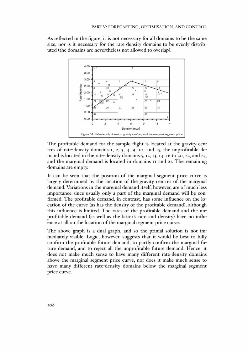
As reflected in the figure, it is not necessary for all domains to be the same size, nor is it necessary for the rate-density domains to be evenly distrib-uted (the domains are nevertheless not allowed to overlap).

The profitable demand for the sample flight is located at the gravity cen-tres of rate-density domains 1, 2, 3, 4, 9, 10, and 15, the unprofitable de-mand is located in the rate-density domains 5, 12, 13, 14, 16 to 20, 22, and 23, and the marginal demand is located in domains 11 and 21. The remaining domains are empty.

It can be seen that the position of the marginal segment price curve is largely determined by the location of the gravity centres of the marginal demand. Variations in the marginal demand itself, however, are of much less importance since usually only a part of the marginal demand will be con-firmed. The profitable demand, in contrast, has some influence on the lo-cation of the curve (as has the density of the profitable demand), although this influence is limited. The rates of the profitable demand and the un-profitable demand (as well as the latter’s rate and density) have no influ-ence at all on the location of the marginal segment price curve.

The above graph is a dual graph, and so the primal solution is not im-mediately visible. Logic, however, suggests that it would be best to fully confirm the profitable future demand, to partly confirm the marginal fu-ture demand, and to reject all the unprofitable future demand. Hence, it does not make much sense to have many different rate-density domains above the marginal segment price curve, nor does it make much sense to have many different rate-density domains below the marginal segment price curve.

10 = cw

2cw

3cw

4cw

5cw

6cw

7cw

8cw

9 cw

00

XI

2 4 96 !18

Density [mc/t]

Cha

rgea

ble

Wei

ght [

cht]



Limiting Factor

Eco

nom

ic P

rope

rty


D sl

r sl

d sl

—yes

—yes

yes—

—yes

—no

yes—


d sl


d sl


d sl


d sl


d sl


d sl


Density Rank

Eco

nom

ic P

rope

rty

D sl

r sl


unfavorable


unfavorableneutral


neutral orfavorable

unfavorabled sl



segment j

2 4 96 !18

Density [mc/t]

Cha

rgea

ble

Wei

ght [

cht]


segment j

10 = cw

2cw

3cw

4cw

5cw

6cw

7cw

8cw

9 cw

0

fc j

10 = cw

bcj

fcj fvcj

fwcj

bwcjbvcj

bcj

fvcj

fwcj

bwcj

bvcj

2 4 96 !18

Density [mc/t]

Cha

rgea

ble

Wei

ght [

cht]


10 = cw

2cw

3cw

4cw

5cw

6cw

7cw

8cw

9 cw

0

fcs fvcs

fwcs

10 = cw

2cw

3cw

4cw

5cw

6cw

7cw

8cw

9 cw

00 2 4 96 !18

Density [mc/t]

Cha

rgea

ble

Wei

ght [

cht]


fcsfvcs

fwcs

0 2 4 96 !18

4.00

3.50

3.00

2.50

2.00

0.50

1.50

1.00

0.00

Density [mc/t]

Rat

e [€

/chk

g]


i=1 2

31 32

25 3029282726

21 242322

15 2019181716

9 1413121110

3 87654

10 = cw

2cw

3cw

4cw

5cw

6cw

7cw

8cw

9 cw

00 2 4 96 !18

Density [mc/t]

Cha

rgea

ble

Wei

ght [

cht]


fcs

bcs

fvcs

fwcs

bwcs

bvcs




s

ss

s


108

However, it does make sense to have as many rate-density domains as pos-sible in the vicinity of the curve in order to be able to delineate the ‘true’ marginal segment price curve as accurately as possible. The crux is that, to do this, the true curve has to be known in advance (which is usually not the case). Nevertheless, if some a priori information is available, this can be used to concentrate the rate-density domains close to the presumed loca-tion of the curve (as has been done in Figure 34).

7.5 Contribution

The first contribution of this chapter is the presentation of two models that can be used to calculate the expected cargo revenue of a single flight that have been set up to use only one quantity unit for their decision vari-ables, their slack variables, and the right-hand sides. Only if the weight, volume, and demand constraints of the primal model are formulated in terms of chargeable kilograms (as proposed in this dissertation) can all the dual values be expressed in euro per chargeable kilogram. To the knowledge of the author, no cargo models have previously been presented that make comparing the weight, the volume, and the demand as easy as the compari-son here between the marginal weight price, the marginal volume price, and the (un)profitability of the demand.

The second contribution is in identifying the three domain states of the rate-density domains that have a positive demand, and in the presentation of the segment-level complementary slackness conditions. The definitions of the free segment capacities and the marginal segment prices, as func-tions of the unified density, are also considered a contribution. The final contribution is the recommendation concerning how to distribute the rate-density domains.

The contributions made in this chapter can also help to answer Karaes-men’s open question as to how to “discretize the weight-volume space to keep the model at a manageable size and the same time realistic.” This question was raised by Karaesmen in her thesis (see Karaesmen 2001, page 60).


109


110

8 Booking Request Control

To successfully manage revenue in air cargo, a fundamental task is to con-firm the ‘right’ booking requests and to reject the ‘wrong’ ones. The ques-tion therefore is in which of these two categories to place a request. Two booking request control methodologies will be presented in this chapter, and both will try to answer this question. However, since it is a contractual obligation of air cargo carriers to fly goods that have been booked, the focus of booking request control is not on the confirmed bookings but on the decision whether to confirm or reject future booking requests as they arrive.

The first booking request control method to be introduced is termed ‘marginal bid price control’, and the second ‘lumpy bid price control’. The difference between them is that marginal bid price control is based on a booking request’s estimated displacement cost, while lumpy bid price control is based on its ‘real’ displacement cost. The displacement cost is also referred to as opportunity cost, and measures the expected revenue loss resulting from using the capacity now rather than reserving it for future use (see Talluri and van Ryzin 2004, pages 32f.; see also Section 3.6 of this dissertation).

Later in this chapter, a booking request control overview scheme will be presented. Such a booking request control overview is unnecessary if the rate, the density, and the size of the actual booking request are known ex-actly, but if these values are only known to lie within certain ranges, a book-ing request control overview can help in reaching the right decision.

The contribution of this chapter will be outlined in the final section.

8.1 Marginal Bid Price Control

The marginal price of an actual booking request is only an estimate of the booking request’s real displacement costs since the marginal price is—in a strict sense—only valid for a booking request that has a marginal (i.e., in-finitesimally small) size. The marginal price depends on the routing of the request, its density (i.e., its weight and volume coefficients), and on the marginal prices of the weight and volume capacities on the traversed legs, whereas the real displacement costs also depend on the actual size of the booking request.

The marginal price of an actual booking request is specified below.

Marginal Price of an Actual Booking Request:mpa0 [0, ∞] [€/chkg]0 marginal price of an actual booking request

111

The definition is as follows:

Marginal Price of an Actual Booking Request as a Function of the Leg Weight and Volume Prices:mpa = ∑l ala wa mwpl + ∑l ala va mvpl

Booking request control on the basis of marginal price is particularly sim-ple and naturally leads to the marginal bid price decision rule shown below.

Marginal ‘Bid Price’ Decision Rule:if0 ra > mpa0 then confirm the actual booking requestelseif0 ra < mpa0 then reject the actual booking requestelseif0 ra = mpa0 then the decision is indeterminate

However, it is worth mentioning that, as Talluri and van Ryzin note, “there need not be a one-to-one correspondence between optimal bid prices and the [estimated] opportunity cost of capacity” (Talluri and van Ryzin 2004, page 92). “That is,” they continue, “one can generate examples of bid prices that give optimal accept or deny decisions but that at the same time are very poor approximations to the marginal value of resource capacity.”

According to Talluri and van Ryzin (ibid., pages 31f.), “a bid-price control sets a threshold price […], such that a request is accepted if its revenue exceeds the threshold price and rejected if its revenue is less than the threshold price.” Further, “in a network setting, a bid price control sets a threshold price—or bid price—for each resource in the network”, as they wrote on page 86, and continued: “This bid price is normally interpreted as an estimate of the marginal cost to the network of consuming the next incremental unit of the resource’s capacity. When a request for a product comes in, the revenue of the request is compared with the sum of the bid prices of the resources required by the product. If the revenue exceeds the sum of the bid prices, the request is accepted; if not, it is rejected.”

Marginal bid price controls have become quite popular among passenger airlines as a method of confirming or rejecting actual booking requests on the basis of their estimated displacement costs. “Bid-price controls have many advantages”, write Talluri and van Ryzin (2004, page 86), and con-tinue “First, even in a network setting the structure of the control remains simple: we have to specify only a single value for each resource (not each product), so the number of parameters involved is minimal. Second, evalu-ating a request for a product requires only a simple comparison of revenue to the sum of bid prices for the requested resources, so the transaction-processing task is quick. Third, bid prices are intuitive and have a natural economic interpretation as the marginal cost to the network of each re-source. Finally, if implemented correctly, bid prices have very good revenue performance and can even be shown to be theoretically near-optimal under certain conditions.”


112

In air cargo, however, such a marginal bid price decision rule might be in-appropriate. The first disadvantage is that it does not consider the size of the booking request because the underlying assumption is that the actual booking request displaces only future demand that has a zero profitability (the term ‘profitability’ is used here as it was defined in Sections 2 and 3 of Chapter 7). The rule’s second disadvantage is that it does not consider the limits of the bookable capacity, so may suggest confirming a booking re-quest that is too large to fit into the remaining capacity (although this dis-advantage can be avoided by an a priori check on bookable capacity). The third disadvantage of the marginal bid price decision rule is that if the dual model has multiple optimal solutions, the bid price may not be uniquely defined (see Popescu 1999, page 109). Finally, the marginal bid price deci-sion rule does not indicate what to do if the rate of the actual booking re-quest is equal to its marginal price, even though this could easily be avoided by using additional decision criteria.

Among the aforementioned drawbacks of using the marginal bid price, the first can be the most damaging since, as Talluri and van Ryzin (2004, pages 32f.) put it, “… capacity should be allocated to a request if and only if its revenue is greater than the value of the capacity required to satisfy it”, and the value of displaced capacity should be measured by its expected dis-placement cost. Further: “Large relative changes in capacity on several re-sources simultaneously cannot, in general, be expected to produce the same revenue effect as the sum of the individual changes” because the bid prices may “fail to capture the opportunity cost” if the “future revenues […] de-pend in a highly nonlinear way on the displaced capacity” (ibid., page 91)—as indeed they do in Network (and Cargo) Revenue Management.

Another criticism of bid price-based booking request control is that in or-der “to be effective, bid prices must be updated after each sale—and possi-bly also with time as well” (Talluri and van Ryzin 2004, page 32). While it is true that bid price updates might be needed to make up for inaccurate de-mand forecasts, bid prices will tend to be constant over time if the forecast is perfect. Talluri and van Ryzin in fact state a similar conclusion on page 120 (ibid.) but, since they refer to the optimisation and control process only, they do not explicitly mention the dominant influence of the forecast quality. Instead, they show that marginal bid price control is asymptotically optimal if the demand volumes and leg capacities tend to infinity (see Tal-luri and van Ryzin 1998).

For all practical purposes, this asymptotic optimality translates into a re-quirement for booking requests to be small relative to the offered capacity. However, this requirement is rarely fulfilled in the airfreight industry since the available capacity is often very limited and because the capacity con-sumed by a booking request can be quite high.

8 BOOKING REQUEST CONTROL

113

For further discussion on the quality of bid price control, see Talluri and van Ryzin (1998) and Talluri and van Ryzin (2004).

8.2 Lumpy Bid Price Control

The main limitations of marginal bid price control can be overcome by applying lumpy bid price control. This form of control not only considers the size of the actual booking request but also the limits of the bookable capacity. Lumpy bid price control is a way of implementing an integer booking request control by comparing the flight revenue that could be achieved by confirming an actual booking request with the flight revenue that might be achieved by not confirming the actual booking request. A similar model has been suggested for airline passenger group bookings by Svrcek (1991, pages 74f.).

Before discussing lumpy bid price control in detail, some preparatory steps have to be taken; the first step being to introduce the concept of booking-reduced flight revenue.

Booking-Reduced Flight Revenue:brfra0 [– ∞, ∞] [€]0 0 flight revenue with booking-reduced0 0 0 0 leg weight and volume capacities

The booking-reduced flight revenue, brfra, is the revenue which could have been earned by filling the booking-reduced bookable leg weight and vol-ume capacities of a flight with profitable future booking requests. These reduced capacities are calculated as the flight’s bookable capacities less the weight and volume consumed by the actual booking request. The booking-reduced bookable weight and volume capacities of a flight leg are defined as bwcl – alawaqa and bvcl – alavaqa.

The booking-reduced capacities do not follow the usual non-negativity constraint because these capacities can be negative if the actual request is larger than the bookable capacity.

The reduced flight revenue can be calculated by solving either mathemati-cal program MP 1 or mathematical program MP 2, with the reduced book-able weight and volume capacities in place. By comparison, fr is the flight revenue which could be earned by filling the unreduced (i.e., bookable) ca-pacities with profitable future booking requests.

The main reason for computing the reduced flight revenue is to be able to calculate the lumpy price of an actual booking request. The lumpy price of an actual booking request is detailed below.

Lumpy Price of an Actual Booking Request:lpa0 [0, ∞] [€/chkg]0 lumpy price of an actual booking request


114

The value range needs to include infinity because if an actual booking request does not fit into the bookable capacity, its lumpy price will be infinite.

Lumpy Price of an Actual Booking Request as a Function of Demand:lpa = (fr – brfra)/qa

More specifically, the lumpy price of an actual booking request will be infi-nite if the request does not fit into the bookable capacity because, then, at least one of the reduced leg capacities has a negative value and the primal model used to calculate the reduced flight revenue becomes infeasible.

The lumpy price of an actual booking request can be used to construct a lumpy bid price decision rule as follows:

Lumpy Bid Price Decision Rule:if0 ra > lpa00 then confirm the actual booking requestelseif0 ra < lpa00 then reject the actual booking requestelseif0 ra = lpa00 then the decision is indeterminate

Again, the uncertainty that exists if the rate of the actual booking request is equal to its lumpy price can be resolved either arbitrarily or by using ad-ditional decision criteria.

8.3 Booking Request Control Overview

A booking request control overview shows an actual booking request in re-lation to the general flight situation. The booking request control overview links the primal graph with the dual graph, adds the bookable segment ca-pacity curve and the full segment price curve, and results in the so-called primal-dual graph. However, before the primal-dual graph and its primal-dual modes can be discussed, some preparatory work is necessary.

The Primal Graph with Free and Bookable Segment Capacities

A primal graph can be enhanced not only by showing the free segment ca-pacity (as was the case in Figures 29 and 30), but also by showing the book-able segment capacity.

The bookable capacity of a segment is the capacity available to accommo-date bookings requested for that particular segment from now until seg-ment departure. It is, as with the free segment capacity, a function of the unified density.

Bookable Segment Capacity:bcs0 [0, ∞) [chkg]0 0 bookable capacity of flight segment s

The calculation of bookable segment capacity is analogous to that of free segment capacity (see the first section of Chapter 7 for details on how to calculate free segment capacity). The free segment weight and volume capacities, fwcs and fvcs, must be replaced by the bookable segment weight


115

and volume capacities bwcs and bvcs, and the resulting segment capacity is, of course, not the free segment capacity fcs but the bookable segment ca-pacity bcs.

Since the bookable segment weight and volume capacities have not yet been defined, they are introduced below.

Bookable Segment Weight and Volume Capacities:bwcs0 [0, ∞) [chkg]0 0 bookable weight capacity of flight segment sbvcs0 [0, ∞) [chkg]0 0 bookable volume capacity of flight segment s

The calculation of the bookable segment weight and volume capacities is again very similar to the calculation of the free segment weight and volume capacities. The definitions of bookable segment weight and volume capaci-ties are given below.

Bookable Segment Weight and Volume Capacities as a Function of the Bookable Leg Weight and Volume Capacities:bwcs = min {bwcl, ∀ l where als = 1}bvcs = min {bvcl, ∀ l where als = 1}

A sample graph showing not only free but also bookable segment capacities is provided in Figure 35.

The sample graph also shows the primal modes. The primal modes are so-called because they refer to the quantity-based primal models that are available to calculate the flight revenue.

The first primal mode covers the area above the free segment capacity (fcs) and gives an indication of what size (or, more specifically, what demand) an actual booking request can have without displacing any likely future de-mand. The second primal mode covers the area between the free segment capacity (fcs) and the bookable segment capacity (bcs) and gives an indica-tion of the size of an actual booking request that could possibly be accept-able, while the third primal mode indicates the size and density of booking

10 = cw

2cw

3cw

4cw

5cw

6cw

7cw

8cw

9 cw

00

XI

2 4 96 !18

Density [mc/t]

Cha

rgea

ble

Wei

ght [

cht]



Limiting Factor

Eco

nom

ic P

rope

rty


D sl

r sl

d sl

—yes

—yes

yes—

—yes

—no

yes—


d sl


d sl


d sl


d sl


d sl


d sl


Density Rank

Eco

nom

ic P

rope

rty

D sl

r sl


unfavorable


unfavorableneutral


neutral orfavorable

unfavorabled sl



segment j

2 4 96 !18

Density [mc/t]

Cha

rgea

ble

Wei

ght [

cht]


segment j

10 = cw

2cw

3cw

4cw

5cw

6cw

7cw

8cw

9 cw

0

fc j

10 = cw

bcj

fcj fvcj

fwcj

bwcjbvcj

bcj

fvcj

fwcj

bwcj

bvcj

2 4 96 !18

Density [mc/t]

Cha

rgea

ble

Wei

ght [

cht]


10 = cw

2cw

3cw

4cw

5cw

6cw

7cw

8cw

9 cw

0

fcs fvcs

fwcs

10 = cw

2cw

3cw

4cw

5cw

6cw

7cw

8cw

9 cw

00 2 4 96 !18

Density [mc/t]

Cha

rgea

ble

Wei

ght [

cht]


fcsfvcs

fwcs

0 2 4 96 !18

4.00

3.50

3.00

2.50

2.00

0.50

1.50

1.00

0.00

Density [mc/t]

Rat

e [€

/chk

g]


i=1 2

31 32

25 3029282726

21 242322

15 2019181716

9 1413121110

3 87654

10 = cw

2cw

3cw

4cw

5cw

6cw

7cw

8cw

9 cw

00 2 4 96 !18

Density [mc/t]

Cha

rgea

ble

Wei

ght [

cht]


fcs

bcs

fvcs

fwcs

bwcs

bvcs




s

ss

s


116

requests that would be too large to accommodate. Hence, primal mode 3 reflects demand-density combinations of actual booking requests which are not feasible, primal mode 2 refers to demand-density combinations which are feasible, and primal mode 1 refers to demand-density combinations which are definitely feasible. The difference between ‘feasible’ and ‘defi-nitely feasible’ is that a definitely feasible actual booking request can be confirmed without having to run a separate lumpy bid price optimisation if its rate is greater than (or equal to) zero.

The following explanation illustrates how a booking request can fall into primal modes 1, 2, or 3. If the density of an actual booking request is 18 cu-bic metres per tonne, and its demand is between cw1 and cw3, the booking request is located in the upper part of Figure 35 and its primal mode is 1. If the booking request has the same density but its demand is between cw3 and cw8, the booking request is located in the middle band and its primal mode is 2. Finally, if the density of the booking request is still 18 cubic me-tres per tonne but its demand is greater than cw8, the booking request is located in the lower part of the figure and its primal mode is 3.

The Dual Graph with Marginal and Full Segment Prices

The dual graph can also be enhanced. This is achieved by not only showing the marginal segment price (as was the case in Figures 32 and 33 above), but by also including the full segment price.

The full segment price is the minimum price necessary to confirm an actual booking request, no matter how large it is (as long as it fits into the book-able capacity). Since this is clearly a what-if simulation, the aforementioned booking request has only a hypothetical nature and its size (i.e., its de-mand) is assumed to be equal to the bookable segment capacity. The full segment price, which is a function of the unified density, is explained below.

Full Segment Price:fps0 [0, ∞] [€/chkg]0 full price of flight segment s

The full segment price is a ‘lumpy price’, defined as the difference between the flight revenue and the segment-reduced flight revenue, divided by the bookable segment capacity. The full segment price is, in many ways, similar to the marginal segment price, except that the marginal segment price is the capacity access price for the smallest possible booking request (i.e., an infinitesimally small one) while the full segment price is the capacity access price for the largest possible booking request (i.e., one that fills the book-able segment capacity). The full segment price is therefore defined as be-low.

Full Segment Price as a Function of Possible Demand:if0 bcs = 000 then fps = ∞elseif0 bcs > 000 then fps = (fr – srfrs)/bcs


117

The full segment price of the largest possible booking request with a zero density is called the full segment weight price fwps, while the full segment price of the largest possible booking request with an infinite density is called the full segment volume price fvps.

The calculation of the full segment price is based on the segment-reduced flight revenue, and this revenue is explained below.

Segment-Reduced Flight Revenue:srfrs0 [0, ∞] [€]0 0 flight revenue with segment s reduced leg capacities

The segment-reduced flight revenue srfrs is the revenue which can be earned by filling the segment-reduced bookable leg weight and volume ca-pacities of a flight with profitable future booking requests. The segment-reduced flight revenue can be calculated by solving either the mathematical program MP 1 or the mathematical program MP 2 but, naturally, with the segment-reduced bookable leg weight and volume capacities used in place of the bookable leg weight and volume capacities.

The segment-reduced bookable leg weight and volume capacities can be calculated for various densities as the flight’s bookable capacity minus the weight and volume consumption of the largest possible booking request that can be accommodated for the given segment at the given density. The segment-reduced bookable weight and volume capacities of a flight leg are defined as bwcl – alsωsbwcs and bvcl – alsνsbvcs.

Since the segment-reduced bookable leg weight and volume capacities de-pend on the assumed density at which the largest possible booking request is calculated, not only the segment-reduced capacities are a function of the unified density but also the segment-reduced flight revenue.

The terms ‘alsωsbwcs’ and ‘alsνsbvcs’ describe the weight and volume con-sumptions of the largest possible booking request that would fit into the bookable capacity of the segment and so, if such a hypothetical booking request were to be confirmed, the respective bookable segment capacity at the given density would be reduced to zero. Hence, the remaining bookable leg weight and volume capacities have been given the label ‘segment-reduced’, and the scalars ωs and νs act as reducing factors that implicitly de-termine the size and the density of the segment’s ‘largest possible booking request’. The reduction factors are formally defined below.

Weight and Volume Reduction Factors:ωs0 [0, 1] [unitless]0 flight segment s weight reduction factorνs0 [0, 1] [unitless]0 flight segment s volume reduction factor

It is, hopefully, apparent that not all combinations of ωs and νs are permit-ted. In order to maintain the full segment capacity reduction, and to vary only the unified density of the largest possible booking request, either ωs has to be equal to 1, and νs to vary parametrically between 0 and 1; or νs has


118

to be equal to 1 with ωs varying parametrically between 1 and 0. Conse-quently, the resulting density uds is defined as follows.

Unified Density of the Largest Possible Booking Request:if0 ωs bwcs = 0 and νs bvcs = 00 0 0 then uds is indeterminateelseif0 ωs bwcs > 0 and (νs bvcs)/(ωs bwcs) ≤ 10 then uds = (νs bvcs)/(2ωs bwcs)elseif0 ωs bwcs > 0 and (νs bvcs)/(ωs bwcs) > 10 then uds = 1 – (ωs bwcs)/(2νs bvcs)elseif0 ωs bwcs = 0 and (νs bvcs) > 00 0 then uds = 1

The maximum values of ωsbwcs and νsbvcs are, of course, equal to bcs.

The determination of the full segment price is, in some senses, a ‘reversed’ lumpy bid price decision rule because it does not ask whether a rate is high enough to be confirmed but, rather, which rate is high enough to be con-firmed. However, the analogy stops here because the full segment price does not refer to an actual booking request (which has a certain size and density), but to the largest possible booking request (which could be a range of sizes, depending on the assumed density).

The full segment price can then be added to the dual graph, as in Figure 36.

This sample graph also includes some dual modes. The dual modes are so-called because they refer to the price-based dual models that can be used to calculate flight revenue.

The first dual mode (1) covers the area above the full segment price (fps) and gives an indication of what rate an actual booking request must have to be able to displace all future demand. The second dual mode (2) covers the area between the full segment price (fps) and the marginal segment price (mps) and indicates the rates at which an actual booking request should be considered, while the third dual mode (3) gives an indication of the rates and densities that would make an actual booking request unacceptable be-cause it would be too cheap to be confirmed. Hence, dual mode 3 reflects the rate-density combinations of an actual booking request that are unprof-

mpsmwps mvps

XX

Varia

ble

density[mc/t]

(revenue)[€]

revenue[€]

revenue[€]

rate[€/kg]

weight[kg]

(volume)[mc]

weight[kg]

weight[kg]

volume[mc]

density[mc/kg]

weight[kg]

–> derivedinitial


Properties


0 1/12 1/6 1/4 1/3 5/12 1/2


Cha

rgea

ble

Wei

ght [

chkg

]

1.0

0.8

0.6

0.4

0.2

0

6

CD

0 1 32 54

void

void

Density [mc/t]

BCAB

CD'

BC'

AB'

volume c

onsumptio

n

weight consumption



Cha

rgea

ble

Wei

ght [

chkg

]1.0

0.8

0.6

0.4

0.2

0

6

void

void

Density [mc/t]

7 98 1110 12

FGEFDE

FG'EF'

DE'

0.5 0.75

weight consumption

volume consumption

8/117/106/95/84/7


0 10 20 30 40 6050

4.00

3.50

3.00

2.50

2.00

0.50

1.50

1.00

0.00


Rat

e [€

/chk

g]

qis

ris fwcl

sisxis

fr


0 10 20 30 40 6050

4.00

3.50

3.00

2.50

2.00

0.50

1.50

1.00

0.00


Rat

e an

d C

ost [

€/c

hkg]

qis

ris

pis

uis

mwpl

fr

bwclbwcl

mps

2 4 96 18

Rat

e [€

/chk

g]


Density [mc/t]

9r

8r

7r

6r

5r

4r

3r

2r

1 0 = r

0 !

mwps

mvps

fps

fvps




10 = cw

2cw

3cw

4cw

5cw

6cw

cwharg

eabl

e W

eigh

t [ch

t]

bcsbwcs

mps

Rat

e [€

/chk

g]

9r

8r

7r

6r

5r

4r

3r

2r

1 0 = r

mwps

mvps

fp

a

a

s

fvps


profitable

not profitable

feasible

rActual Booking

Request


q10 = cw

2cw

3cw

4cw

5cw

6cw

cwharg

eabl

e W

eigh

t [ch

t]

bcsbwcs

Rat

e [€

/chk

g]

9r

8r

7r

6r

5r

4r

3r

2r

1 0 = r

fps

fvps


profitable

feasible

fcsfvcs

fwcs

definitely feasible



fvcsfwcs fcs

s

a

ar

q


119

itable, dual mode 2 covers the rate-density combinations which are profit-able, and dual mode 1 refers to the rate-density combinations which are definitely profitable. The difference between ‘profitable’ and ‘definitely profitable’ is that a definitely profitable actual booking request can be con-firmed without having to run a separate lumpy bid price optimisation if its demand is less than (or equal to) the bookable segment capacity.

It is useful to show here how a booking request can fall into dual modes 1, 2, or 3. If the density of an actual booking request is 18 cubic metres per tonne, and if its rate is between r1 and r3, the booking request is located in the lower part of Figure 36 and its dual mode is 3. If the booking request has the same density but its rate is between r3 and r5, the booking request is located in the middle band and its dual mode is 2. Finally, if the density of the booking request is still 18 cubic metres per tonne but its rate is greater than r5, the booking request is located in the upper part of the figure and has a dual mode of 1.

The Primal-Dual Graph

The primal-dual graph (or the booking request control overview as it is also known) is a combination of the primal and the dual graphs, with the dual graph being shown above the primal one. This combination not only re-flects the complementarity between the marginal price of a segment and its free capacity, but also leads to a common zero reference line (i.e., the den-sity axis).

Further, it also makes sense to include the rate, the density, and the demand of the actual booking request in the primal-dual graph so as to be able to compare the features of the booking request with what is required to obtain a confirmation. The possibility of comparing the actual rate, density, and demand with the ‘required’ rate, density, and demand can be of great help in steering sales.

Two examples of primal-dual graphs are shown below. The first example (Figure 37 on Page 121) shows a free segment capacity (fcs) of zero, a mar-ginal segment price (mps) that fluctuates between r2 and r4, a bookable seg-ment capacity (bcs) that runs from cw6 to cw8, and a full segment price (fps) that takes a value between r5 and r8. The demand of an actual booking re-quest qa and its rate ra are also pictured. As can easily be seen, the demand of the actual booking request fits into the bookable segment capacity, but the rate of the request is less than the marginal segment price. Hence, the actual booking request is feasible but not profitable, and should therefore be rejected.


120

The situation is slightly different in the second example (Figure 38 on Page 122). In this primal-dual graph, it is the marginal segment price that is zero while the free segment capacity varies between cw3 and cw4. The bookable segment capacity, however, has not changed (nor has the full segment price). The demand and the rate of the actual booking request are also taken to be the same as in the previous figure.

Since the actual booking request in Figure 38 is not only ‘profitable’ but also ‘definitely feasible’, it can be confirmed right away without running a separate lumpy bid price calculation. This is because the outcome of the lumpy bid price decision rule can, at least in some cases, be foreseen by looking at the applicable primal and dual modes—with the applicable pri-mal mode reflecting the demand of the actual booking request and the ap-plicable dual mode referring to its rate.

XX

mpsmwps mvps

10 = cw

2cw

3cw

4cw

5cw

6cw

7cw

8cw

9 cw

00 2 4 96 !18

Density [mc/t]

Cha

rgea

ble

Wei

ght [

cht]

Figure 37: Primal-dual graph with an unprofitable booking request

bcsbwcs

bvcs

mps

Rat

e [€

/chk

g]

9r

8r

7r

6r

5r

4r

3r

2r

1 0 = r

mwps

mvps

fp

a

a

s

fvps


profitable

not profitable

not feasible

feasible

rActual Booking

Request


q10 = cw

2cw

3cw

4cw

5cw

6cw

7cw

8cw

9 cw

00 2 4 96 !18

Density [mc/t]

Cha

rgea

ble

Wei

ght [

cht]

Figure 38: Primal-dual graph with a definitely profitable booking request

bcsbwcs

bvcs

Rat

e [€

/chk

g]

9r

8r

7r

6r

5r

4r

3r

2r

1 0 = r

fps

fvps


profitable

not feasible

feasible

fcsfvcs

fwcs

definitely feasible



fvcsfwcs fcs

ss

a

ar

q


121

An overview of the possible primal-dual mode combinations of an actual booking request is given in Figure 39 below.

As has already been explained, the primal modes of a segment are distin-guished by the free segment capacity (fcs) and the bookable segment capac-ity (bcs), while the dual modes of a segment are separated by the marginal segment price (mps) and the full segment price (fps).

XX

mpsmwps mvps

10 = cw

2cw

3cw

4cw

5cw

6cw

7cw

8cw

9 cw

00 2 4 96 !18

Density [mc/t]

Cha

rgea

ble

Wei

ght [

cht]

Figure 37: Primal-dual graph with an unprofitable booking request

bcsbwcs

bvcs

mps

Rat

e [€

/chk

g]

9r

8r

7r

6r

5r

4r

3r

2r

1 0 = r

mwps

mvps

fp

a

a

s

fvps


profitable

not profitable

not feasible

feasible

rActual Booking

Request


q10 = cw

2cw

3cw

4cw

5cw

6cw

7cw

8cw

9 cw

00 2 4 96 !18

Density [mc/t]

Cha

rgea

ble

Wei

ght [

cht]

Figure 38: Primal-dual graph with a definitely profitable booking request

bcsbwcs

bvcs

Rat

e [€

/chk

g]

9r

8r

7r

6r

5r

4r

3r

2r

1 0 = r

fps

fvps


profitable

not feasible

feasible

fcsfvcs

fwcs

definitely feasible



fvcsfwcs fcs

ss

a

ar

q

( )smp

( )sfp

s( )fc s( )bc

!

VI

reject

reject

reject

Figure 39: Primal–dual modes and an actual booking request

Primal Mode

Dua

l Mod

e

1 2 3

reject

confirm

optimise

1

2

3

not feasiblefeasibledefinitely feasible


confirm

confirm

optimise

Confirmation of a booking request. Case 3: fcs = 0, bps = 0


Pric

e [e

uro/

chkg

]

no

yesno

no

no

0fcs 0acs

0

bps 0

aps

yes

yes

not possible

optimise

Confirmation of a booking request. Case 1: fcs > 0, bps = 0


Pric

e [e

uro/

chkg

]

no

yesno

no

no

0fcsacs

0

bps 0

aps

yes

yes

not possible

0

optimise

Confirmation of a booking request. Case 2: bps > 0, fcs = 0


Pric

e [e

uro/

chkg

]

no

yesno

no

no

fcs 0acs

bps

aps

yes

yes

not possible

0

Size, rate and the confirmation of a booking request


Pric

e [e

uro/

chkg

]

0fcsacs

0

bps

aps

0 2 4 96 18

4.00

3.50

3.00

2.50

2.00

0.50

1.50

1.00

0.00

Density [mc/t]

Pric

e [e

uro/

chkg

]

Volume Stowage Loss, Rate and Density

! 0 2 4 96 18

0

1

2

3

4

7

5

6

8

Density [mc/t]

Cha

rgea

ble

Wei

ght [

cht]

Volume Stowage Loss, Demand and Density

300

200

100d

D = f (d )slsl

max dsl

0 10080604020 0 10080604020

d

r = f (d )slsl

max dsl

Volume S

towage Loss [%

]

300

200

100

Volume S

towage Loss [%

]

(!)(0)

(0)

(!)

reject

reject

reject

Figure 46: Primal–dual modes and an actual booking request with stowage loss

Primal Mode

Dua

l Mod

e

1 2 3

reject

confirm

optimise

1

2

3

confirm

confirm

(!)(0)

(0)

(!)

( )smp

( )sfp

s( )fc s( )bc

notprofitable

profitabledefinitelyprofitable

notprofitable



122

In addition to these values, the zero values (“0”) and the infinite values (“∞”) are also included to ease understanding.

Since, at a given density, the marginal price of a segment and its free seg-ment capacity cannot both be positive at the same time (at least not in an optimal solution), the primal-dual mode (1:3) cannot exist. Moreover, the actual options among the remaining primal-dual modes can be further re-duced since some modes may have only a virtual existence. If, for example, the free segment capacity at a given density is zero, primal mode 1 cannot exist and the primal-dual modes in the first column are not an option. Hence, the second column has to start with fcs = 0 and the only available primal-dual modes are (2:1), (2:2), (2:3), (3:1), (3:2), and (3:3).

Turning to the previously discussed flight situations, the actual booking request shown in Figure 37 was rejected because it fell into primal-dual mode (2:3), and the actual booking request of Figure 38 was confirmed be-cause it fell into primal-dual mode (1:2).

The primal-dual graph of another typical flight situation is shown in Figure 40 on Page 124. In this example, the flight segment has less bookable vol-ume than it has bookable weight, and there is a greater demand for volume than there is for weight. In this situation, the flight is expected to have some free segment weight capacity but no free segment volume capacity.

The rate and the density of an actual booking request are also shown but, even though the request is both ‘profitable’ and ‘feasible’, this is no guaran-tee of being confirmed. Here, the final decision will depend on a revenue optimisation procedure and the outcome of the lumpy bid price decision rule because the actual booking request falls into primal-dual mode (2:2), indicating that it needs to be ‘optimised’ (see the confirm, optimise, and reject recommendations of Figure 39).


123

Clearly, such conclusions are based on the precalculation of several scenar-ios, and so neither computational time nor computational effort are saved. However, the primal-dual graph and its primal-dual modes are a convenient way to put an actual booking request into perspective and to visualise any changes that are needed to confirm it.

8.4 Contribution

The contribution of this chapter is in the presentation of the booking re-quest control overview. More specifically, the contribution is seen as the primal-dual graph with the associated primal-dual modes, including the dis-play of the various segment capacities and segment prices as a function of the unified density.

s

bwcs

bvcs

mpsmvps

fpsfvps

fwps

fcsfvcs

fwcs bc

estsl

estsl

XXI

10 = cw

2cw

3cw

4cw

5cw

6cw

7cw

8cw

9 cw

00 2 4 96 !18

Density [mc/t]

Cha

rgea

ble

Wei

ght [

cht]

Figure 40: Primal-dual graph for a volume-restricted flight segment

Rat

e [€

/chk

g]

9r

8r

7r

6r

5r

4r

3r

2r

1 0 = r

definitelyprofitable

lowdemand

highdemand

profitable

not profitable

not feasible

feasible

defin

itely

feas

ible



Flig

ht R

even

ue [e

uro]

A multi-graph of a flight with a high demand


9rf

8rf

7rf

6rf

5rf

4rf

3rf

2rf

1 0 = rf

2cw 3cw 4cw 5cw 6cw 7cw1 0 = cw

First ComeFirst Serve

FractionalPerfect

HindsightBookingRequestControl

Flig

ht R

even

ue [e

uro]

A parametric variation of a marginal leg weight (or volume) price

Marginal Leg Weight (Volume) Price [euro/chkg]

9rf

8rf

7rf

6rf

5rf

4rf

3rf

2rf

1 0 = rf

1k0 = m…p km…p2 km…p

3 km…p4 km…p

5 km…p6 km…p

7

Sto

wag

e Lo

ss R

ange

sFl

ight

Rev

enue

[eur

o]

A multi-graph of a flight with a low demand


9rf

8rf

7rf

6rf

5rf

4rf

3rf

2rf

1


nolo

ss

Rev

enue

Pot

entia

l

Rev

enue

Pot

entia

lye

sga

in


FractionalPerfect

Hindsight

BookingRequestControl

10 = cw

2cw

3cw

4cw

5cw

6cw

7cw

8cw

9 cw

00 2 4 96 !18

Density [mc/t]

Cha

rgea

ble

Wei

ght [

cht]

Figure 45: Primal-dual graph with a booking request and stowage loss

Rat

e [€

/chk

g]

9r

8r

7r

6r

5r

4r

3r

2r

1 0 = r


profitable

not profitable

not feasible

feasible

defin

itely

feas

ible


qsl

optimise

Figure 48: Various booking requests and their stowage loss range

fc

optimise

rejectconfirm

fp mpbc


7sl6sl5sl4sl3sl2sl

reject

mp

0 = rf

rActual Booking

Request

maxsl

maxsl

rejectconfirm

mpbc

reject

fp

0 = 1sl

sdc

bc

fp

mp

sdc

fp

mp

bc

ss

s

bwcs

bvcs

mps

mwpsmwps

mvps

fpsfvps

fwps

fcsfvcs

fwcs bc

ar

aq

a

aa

aaq

a

rsla


124

9 Booking Request Control with Stowage Loss

In the first section of this chapter, a short overview of the phenomenon known as ‘stowage loss’ will be given. The second major topic of this chap-ter is the influence of stowage loss on the initial and derived properties of a booking request. Then, a mathematical program is presented to calculate the maximum acceptable stowage loss of a booking request and subse-quently the primal-dual graph, which has already been introduced, will be extended to display the consequences of stowage loss. Finally, a so-called stowage loss bar is introduced. The chapter then concludes with a consid-eration of its contribution to the subject field.

9.1 Volume Stowage Loss

In theory, a shipment can create two types of stowage loss: volume stowage loss and weight stowage loss. However, whereas the phenomenon of vol-ume stowage loss is well known in the literature (the term ‘stowage loss’ is generally used to refer to volume stowage loss), weight stowage loss is less well known. To give an example of weight stowage loss, one can think of a heavy shipment which can only be transported in the front of a plane. Clearly, to balance the plane, it is necessary to also place heavy freight in the back of the airplane. However, if no heavy freight has been booked that can be transported in the back of the plane, some other weight has to be loaded—and this other weight constitutes a weight stowage loss. Volume stowage loss, however, is far more common and, therefore, weight stowage loss will not be considered any further.

The Reasons for Volume Stowage Loss

The main reasons for stowage loss are the unusual dimensions or the spe-cial contours of a shipment. However, the size and the availability of load-ing devices, the aircraft type, and a shipment’s special handling codes may also be factors. Some of the reasons behind the stowage loss of a shipment are explained in more detail below.

❖ Size of loading devices.

Loading devices are needed to move shipments on and off an air-plane and to secure them within it. There is a wide variety of loading devices, such as the PAG/PAJ pallet, with a usable loading area of304 × 210 centimetres (length × width) and a maximum gross weight of 6,804 kilograms, and the AKH container, with internal dimensions of 146 × 144 × 111 centimetres (length × width × height), a usable volume of 3.4 cubic metres, and a maximum gross weight of 1,134 kilograms.

125

For a large air cargo carrier, it is not unusual to deal with up to 50 different types of loading devices. However, if a loading device blocks more space than it needs (or more positions), it then causes a volume stowage loss.

❖ Aircraft types.

Despite the large variety of loading devices, the choice may be limited on a particular aircraft type. For example, a PAG/PAJ pallet is not loadable onto a Boeing 737 aircraft, possibly meaning that a loading device of unfavourable dimensions has to be chosen if the shipment must use that flight and no better loading device is available. Quite often it is very difficult to identify a single reason for stowage loss; in the given example, the stowage loss is caused by an unsuitable loading device / aircraft type combination.

❖ Special handling codes.

The special handling codes of a shipment can also have a major impact on its stowage loss. Dangerous goods (special handling code DGR), for example, need to be freely accessible in the airplane.

To make matters worse, it is possible that the stowage loss of a particular shipment depends not only on its own dimensions and its own contours, but also on the dimensions and the contours of other shipments. Here, however, it is assumed that the stowage loss of a particular shipment is in-dependent of any other booking for the following reasons:

❖ Since the stowage loss of an actual booking request depends not only on the bookings which have already been confirmed but also on the bookings which will be confirmed within the remaining booking period, a good forecast of the dimensions and the contours of the future freight would be needed in order to calculate the cor-rect amount of stowage loss for the actual booking request. However, it is virtually inconceivable that a sufficiently accurate forecast will ever exist due to the inherent complexities and uncertainties inforecasting dimensions and contours.

❖ To calculate the stowage loss of an actual booking request prior to departure, the complete load planning process (including a process which is called ‘weight and balance’) would have to be simulated. However, this task is not only time-consuming, it is also unreliable, especially in the early stages of the booking process when only a few bookings have been confirmed and the simulation has to run mainly on the basis of forecast data of future bookings.

Further information about loading devices and stowage loss can be found in O’Connor (2001, pages 188ff.) and in Radnoti (2002, pages 158ff.).


126

The Properties of an Actual Booking Request with Stowage Loss

Prior to a discussion on the effects of volume stowage loss on the initial and derived air cargo properties of an actual booking request, the symbol for stowage loss, its unit, and its value range are introduced below.

Volume Stowage Loss of an Actual Booking Request:sla0 [0, ∞) [chkg]0 0 volume stowage loss of an actual booking request

The economic unit of volume stowage loss is its chargeable weight (or, more specifically, the chargeable kilograms that form the chargeable weight), but its physical unit is, of course, the cubic metre. Since the stow-age loss is both an economic and a technical phenomenon, the chosen unit will depend on the intended use.

Clearly, the volume of a booking request with stowage loss is the sum of its original volume plus its stowage loss, but the volume is not the only prop-erty which may be affected by a stowage loss. A list of the initial and de-rived air cargo properties which are—at least potentially—affected by a volume stowage loss is given below. (For completeness, the weight and the revenue are also included, although these properties are not usually af-fected by a volume stowage loss).

Weight, Volume and Revenue of an Actual Booking Request with Stowage Loss:Wa0 [0, ∞) [kg]0 0 weight of an actual booking request with0 0 0 0 (or without) stowage lossVasl0 [0, ∞) [mc]0 0 volume of an actual booking request with 0 0 0 0 stowage lossRa0 (0, ∞) [€]0 0 revenue of an actual booking request with0 0 0 0 (or without) stowage loss

Derived Air Cargo Properties of an Actual Booking Request with Stowage Loss:rasl0 (0, ∞) [€/chkg]0 rate of an actual booking request with 0 0 0 0 stowage loss; also called effective ratewasl0 [0, 1] [chkg/chkg]0 weight coefficient of an actual booking request0 0 0 0 with stowage lossvasl0 [0, 1] [chkg/chkg]0 volume coefficient of an actual booking request0 0 0 0 with stowage lossdasl0 [0, ∞] [mc/t]0 0 density of an actual booking request with 0 0 0 0 stowage lossudasl0 [0, 1] [unitless]0 unified density of an actual booking request 0 0 0 0 with stowage lossqasl0 (0, ∞) [chkg]0 0 demand (quantity) of an actual booking request0 0 0 0 with stowage loss; also called effective demand

The values of the properties which are affected by stowage loss can be cal-culated using formulas that have already been presented, by substituting the original volume in the formulas by a gross volume that includes the stowage loss.

9 BOOKING REQUEST CONTROL WITH STOWAGE LOSS

127

The Density of a Booking Request with Stowage Loss

The density with stowage loss of an actual booking request, dasl, is, as is the density of every other item in air cargo, defined as a volume divided by a weight. Now, since the weight is not affected, the volume stowage loss increases the density of the booking request—unless, of course, it is already infinite.

In comparison, udasl is the unified density of an actual booking request with stowage loss. A volume stowage loss increases the unified density of a book-ing request (unless its value is already equal to 1).

The Effective Demand and its Effective Rate

The effective demand of an actual booking request, qasl, will also increase with a volume stowage loss, provided the added volume is the ruling factor in the calculation of the chargeable weight. Hence, the effective demand increases only when the density with stowage loss is greater than the stan-dard density.

The effective rate of an actual booking request, rasl, is the counterpart of the effective demand. Since the revenue of an actual booking request is usually unaffected by stowage loss (customers rarely pay for stowage loss), the effective rate of a booking request decreases if its effective demand increases. Hence, the effective rate decreases if the density of a booking request with stowage loss is greater than the density of standard cargo because the effective rate rasl multiplied by the effective demand qasl has to be equal to the product of the original rate ra and the original demand qa.

It is, of course, in the best interests of a carrier to avoid a rate decrease and instead charge the customer for stowage loss. However, in order to charge the customer for stowage loss, a renegotiation of the chargeable weight of the booking request would be required, and the result of such renegotia-tions depends not only on the market situation but also on the negotiation powers of both parties.

The Propagation of Stowage Loss

The effect of stowage loss within the extended set of derived air cargo properties is shown in Figure 41. As has generally been the case with these figures, the precedence of the variables and the flow of calculations are also shown.


128

Items that are affected by a volume stowage loss are indicated by an aster-isk(*).

The Stowage Loss Curves

Table 3 below shows the effects of stowage loss on the properties of three sample booking requests. The original values of the booking request prop-erties are given in the first row of the table, while in each subsequent row an additional ‘provisional’ volume stowage loss of 1.8 cubic metres is added to create a range of situations.

As can be seen from the table, the first booking request had an original density below the standard density, the second booking request had an o-riginal density greater than the standard density but less than infinity, and the third booking request had an infinite density. What can be seen from the table is that the properties of these booking requests behave quite dif-ferently when a volume stowage loss is added.

estsla

estslaamaxsl

critical

qslqsl

dsl

v sl

wsl


stowage loss*

Den

sity

Mix

of T

wo

Item

s [%

]

Uni

fied

Den

sity

Lab

els

0 1 32 54

7.2 6 void

void6

12 9! 36 18

200

166

133

100

Density [mc/t]

Density [mc/t]


–1 –.833 –.5–.66 –.166–.33 0 void


!"


Varia

ble

density withstowage

loss*

revenue

weight

revenue

effectivedemand*


volume withstowage

loss*

weight

revenue


stowage loss*

effectivedemand*

effectiverate*

rasl

–>



Varia

ble

wc[kg/chkg]

tc[kg/t]

chtc[chkg/cht]

tc[kg/t]

tc[kg/t]

tc[kg/t]


ds[mc/t]

vc[mc/cht]

ds[mc/t]

chtc[chkg/cht]

chtc[chkg/cht]

chtc[chkg/cht]

–> derivedinitial



–> derivedinitial


Varia

ble

revenue[euro]

revenue[euro]


volume*[mc]

volume*[mc]

weight[kg]

revenue[euro]



rate*[euro/chkg]


density*[mc/t]

weight[kg]

–> derivedinitial


Properties

Varia

ble

revenue[€]

revenue[€]


volume[mc]

volume[mc]

weight[kg]

revenue[€]

weightcoefficient

[chkg/chkg]


rate[€/chkg]

volumecoefficient

[chkg/chkg]

density[mc/t]

weight[kg]

0 1 32 54 7.2

scaled density

6 129 !3618

0 1 32 54 7

range split: “0 – 6” and “6 – 12”

6 98 121110

w0 w1 w3w2 w5w4 v5


6 v3v4 v0v1v2

0 1 32 54 v5


6 v3v4 v0v1v2

0 1 32 54 – 5


6 – 3– 4 – 0– 1– 2




optimise …


7sl6sl5sl4sl3sl2sl


rejectconfirm

fp mpbc


7sl6sl5sl4sl3sl2sl


fp mpbc

Sto

wag

e Lo

ss R

ange

s

sdc

0 = 1sl0 = 1sl

sdc

aa

a

a

a

amaxsl estsla


volume cost[euro]

VIII





d[mc /t ]

Chargeable

[chkg ]Weight cw

[kg ] [mc ]

………………0.0181.801.000.60103

0.0060.601.000.60101………………

0.0183.001.001.0063

0.0061.001.001.0061………………

0.0003.000.001.00030.0002.000.001.00020.0001.000.001.0001

0.0000.00***0

0.0122.001.001.0062

0.0121.201.000.60102

* indeterminate

!

!!

Weight[kg ]

1.001.00

1.000.660.50

Volume[mc ]

0.0040.003

0.0060.0060.006

v[chkg /chkg ]

0.660.50

1.001.001.00

w

1.001.00

1.000.660.50

][chkg /chkgd

[mc /t ]

43

69

12

Item[–]

IH

JKL


–> derivedinitial


Properties

Varia

ble

volume cost[euro]


volume[mc]

volume[mc]

volume cost[euro]



volumecoefficient

[chkg/chkg]

density[mc/t]

–> derivedinitial


Properties

Varia

ble

weight cost[euro]

weight cost[euro]


weight[kg]

weight cost[euro]

weightcoefficient

[chkg/chkg]



density[mc/t]

weight[kg]

ds4d 5d3d

Density [mc/t]

Rat

e [e

uro/

chkg

]


6r

5r

Dij

xx

xxxi=21 i=22

x) c

harg

eabl

e w

eigh

t boo

king

requ

est

) cha

rgea

ble

wei

ght g

ravi

ty c

ente

r

(Regular Density [mc/t])


(Rate per A

ctual Weight [€

/kg])R

ate

per

Cha

rgea

ble

Wei

ght [

€/c

hkg]


7d6d4d 5d3d2d1d

……

……

Density [mc/t]

Rat

e [e

uro/

chkg

]


……

…

…

…

…

…

…

…

…

…

…

…

…

…

…

…

…

…

…

…

…

…

…

… …

…

…

…

…

… …

…

… …

…

…

…

9r

8r

7r

6r

5r

4r

3r

2r

1r

bookingclass

segment

43

7 …

2

456123

0 0 [chkg]

65

BCoptx max

BCx

j=1

dij

domaindemand

domaindensity

rlbookingrequest

raterijdomain rate

lD



!"#$%&%'$(

)"*+,-.


(o)

(o)

(o)

(o)

(o)

(o)o

o o

o

o

o

o

o

o

o

o

o

"18960

128 104

42

s

620

slv

… …

10.8

9.0

7.2

5.4

3.6

0

6.6

6.0

5.4

4.8

4.23.6

3 1

0.91

… …

3,000

3,0003,000

3,000

3,000

3,000

3,300



3.41

3.75

3.75

3.75

3.75

0.5

1

1

0.9

0.8

0.7

1

1

1

11 0.6 3.75

3.75

" 0 3.41

" 0 3.75 3,000

3,3003,600

3,900

4,200

4,500

4,800

slwdsl r sl qsl

1

1

1

1

11

1

slv

" 0 3.13

" 0 2.88

" 0 2.68

" 0 2.50

" 0 2.34

9.9 0.61 3.41

9 0.67 3.75 3,000

3,3003,600

3,900

4,200

4,500

4,800

slwdsl r sl qsl

1

1

1

1

11

1

slv

10.8 0.56 3.13

11.7 0.51 2.88

12.6 0.48 2.68

13.5 0.44 2.50

14.4 0.42 2.34

sla

1.8


129

More specifically, the properties of the low-density booking request change significantly as soon as its density with stowage loss becomes greater than the standard density.

What can be seen from the sample booking requests presented in Table 3 is that there are three distinct situations with regard to the original density. The situations are: da ≤ sdc, sdc < da < ∞, and da = ∞, or, if being expressed in terms of the unified density uda ≤ 0.5, 0.5 < uda < 1, and uda = 1.

The formulas for the effective rate and the effective demand, as a function of the booking request’s unified density with stowage loss, are given below.

Effective Rate as a Function of Unified Density:if0 0 ≤ uda ≤ 0.50 and uda ≤ udasl < 0.500 then rasl = ra

elseif0 (as above)0 and 0.5 ≤ udasl ≤ 10 0 then rasl = (2 – 2udasl) ra

elseif0 0.5 < uda < 10 and uda ≤ udasl < 10 0 then rasl = ra (1 – udasl)/(1 – uda)elseif0 uda = 100 0 0 0 0 then udasl = 1

Effective Demand as a Function of Unified Density:if0 0 ≤ uda ≤ 0.50 and uda ≤ udasl < 0.500 then qasl = qa

elseif0 (as above)0 and 0.5 ≤ udasl < 10 0 then qasl = qa/(2 – 2udasl)elseif0 (as above)0 and udasl = 10 0 0 then qasl = ∞elseif0 0.5 < uda < 10 and uda ≤ udasl < 10 0 then qasl = qa (1 – uda)/(1 – udasl)elseif0 uda = 100 0 0 0 0 then udasl = 1

Figure 42 shows the effective rates of the aforementioned booking requests as a function of their unified density with stowage loss.

The three sample booking requests can also be used to illustrate the effec-tive demand curves. Figure 43 shows the effective demand of the booking requests as a function of their unified density with stowage loss.

0 2 4 96 18

0

1

2

3

4

7

5

6

8

Density [mc/t]

Cha

rgea

ble

Wei

ght [

cht]

Example 1: Demand breakpoints, density and stowage loss

V

0 2 4 96 18

4.00

3.50

3.00

2.50

2.00

0.50

1.50

1.00

0.00

Density [mc/t]

Pric

e [e

uro/

chkg

]

Rate is not the limiting factor for stowage loss

0 2 4 96 !18

0

1

2

3

4

7

5

6

8

Density [mc/t]

Sla

ck C

harg

eabl

e W

eigh

t [ch

t]

Chargeable weight is the limiting factor for stowage loss

0 2 4 96 !18

4.00

3.50

3.00

2.50

2.00

0.50

1.50

1.00

0.00

Density [mc/t]

Pric

e [e

uro/

chkg

]

Example 2: Rate breakpoints, density and stowage loss

0 2 4 96 18

0

1

2

3

4

7

5

6

8

Density [mc/t]

Cha

rgea

ble

Wei

ght [

cht]


0 2 4 96 18

4.00

3.50

3.00

2.50

2.00

0.50

1.50

1.00

0.00

Density [mc/t]

Pric

e [e

uro/

chkg

]Example 1: Rate breakpoints, density and stowage loss

300 %

100 %

300 %

!

bps j

aps j

bps j

aps j

!

acs j

fcs j

!

acs j

fcs j

!

bps j

aps j

acs j

fcs j

200 %

500 %

100 %

33 %

100 %

100 %

367 %

500 %

833 %

600 %

0 2 4 96 18

4.00

3.50

3.00

2.50

2.00

0.50

1.50

1.00

0.00

Density [mc/t]

Rat

e [€

/chk

g]

Figure 42: Three booking requests and their decreased rate due to stowage loss

!

0 2 4 96 18

0

1

2

3

4

7

5

6

8

Density [mc/t]

Cha

rgea

ble

Wei

ght [

cht]

Figure 43: Three booking requests and their increased demand due to stowage loss

!

r = f (d )slsl

max dsl

max dsl

%sl

%sl

D = f (d )slsl

%sl

%sl

max dsl

max dsl

rr

ThirdBookingRequest

ThirdBookingRequest

Second BookingRequest

First BookingRequest

r

rslr

aaa

a

a a a

aaslrsl

qslqsl qsl

qa qa qa




130

It should be noted that the real driver of the rate and demand modifica-tions is, of course, the stowage loss and not the density. Hence, the effec-tive rate and the effective demand of an actual booking request are driven by the stowage loss, and the density is not a causal variable. Moreover, the density is not even an intermediary variable if its value is infinity (i.e., if uda is equal to 1).

9.2 Stowage Loss and Optimal Flight Revenue

Essentially, there are two ways of looking at the stowage loss of an actual booking request. Either the stowage loss is taken as such, that is, as an added volume, which is unfavourable because of the adverse effects on the optimal flight revenue; or the stowage loss is seen as a simultaneous modi-fication to the rate, the demand, and the density of the actual booking re-quest, that is, as a set of individual modifications which may be favourable or unfavourable by themselves, although the overall effect of stowage loss is, of course, always unfavourable (at least it has that potential).

The issue therefore becomes one of how the rate, the demand, and the density modifications relate to the requirements of the instruments which have been identified as available to increase the revenue of a single flight (see Section 4 of Chapter 4 for a discussion of these instruments).

To answer this question, four distinct cases need to be discussed, and each case must not only analyse the consequences of the individual modifica-tions but also describe their interrelationships.

0 2 4 96 18

0

1

2

3

4

7

5

6

8

Density [mc/t]

Cha

rgea

ble

Wei

ght [

cht]


V

0 2 4 96 18

4.00

3.50

3.00

2.50

2.00

0.50

1.50

1.00

0.00

Density [mc/t]

Pric

e [e

uro/

chkg

]

Rate is not the limiting factor for stowage loss

0 2 4 96 !18

0

1

2

3

4

7

5

6

8

Density [mc/t]

Sla

ck C

harg

eabl

e W

eigh

t [ch

t]

Chargeable weight is the limiting factor for stowage loss

0 2 4 96 !18

4.00

3.50

3.00

2.50

2.00

0.50

1.50

1.00

0.00

Density [mc/t]

Pric

e [e

uro/

chkg

]


0 2 4 96 18

0

1

2

3

4

7

5

6

8

Density [mc/t]

Cha

rgea

ble

Wei

ght [

cht]


0 2 4 96 18

4.00

3.50

3.00

2.50

2.00

0.50

1.50

1.00

0.00

Density [mc/t]

Pric

e [e

uro/

chkg

]


300 %

100 %

300 %

!

bps j

aps j

bps j

aps j

!

acs j

fcs j

!

acs j

fcs j

!

bps j

aps j

acs j

fcs j

200 %

500 %

100 %

33 %

100 %

100 %

367 %

500 %

833 %

600 %

0 2 4 96 18

4.00

3.50

3.00

2.50

2.00

0.50

1.50

1.00

0.00

Density [mc/t]

Rat

e [€

/chk

g]

Figure 42: Three booking requests and their decreased rate due to stowage loss

!

0 2 4 96 18

0

1

2

3

4

7

5

6

8

Density [mc/t]

Cha

rgea

ble

Wei

ght [

cht]

Figure 43: Three booking requests and their increased demand due to stowage loss

!

r = f (d )slsl

max dsl

max dsl

%sl

%sl

D = f (d )slsl

%sl

%sl

max dsl

max dsl

rr

ThirdBookingRequest

ThirdBookingRequest



r

rslr

aaa

a

a a a

aaslrsl

qslqsl qsl

qa qa qa




131

Stowage Loss and Instruments to Increase Flight Revenue

The four cases that are needed to analyse the consequences of the individ-ual modifications to the instruments which are available to increase the revenue of a single flight, and to describe their interrelationships, are pre-sented next.

❖ da < dasl ≤ sdc: Both densities of the actual booking request, its original density da, and its density with stowage loss dasl, are ‘high’.

Within this range, stowage loss affects neither the effective rate of the booking request nor its effective demand. Thus, the unfavourableaspect of the stowage loss is only attributable to the fact that, due to the stowage loss, the density of the booking request becomes closer to the density of standard cargo.

In terms of the instruments which are available to increase the rev-enue of a flight, such stowage loss is unfavourable because it limitsthe mix of high and low densities by turning a high-density booking request into one which is closer to the standard density.

❖ da < sdc < dasl: The original density of the actual booking request is ‘high’, whereas its density with stowage loss is ‘low’.

Within this range, no general statement about the overall favour-ability of the density modification can be made. Initially, increasing the stowage loss means moving the density of the booking request closer to the standard density (which is unfavourable) but, subse-quently, after having passed the standard density, a further increase in stowage loss means moving away from the standard density (which is favourable). However, as soon as the density with stowage loss becomes lower than the standard density, the effective rate of the booking request will decrease—and low effective rates tend to be unfavourable with the instruments that are available to increase the flight revenue.

❖ sdc ≤ da < dasl: The two densities of the actual booking request, i.e.,with and without stowage loss, are ‘low’.

Here, the original density of the booking request is already lower than the standard density, and so an already favourable low-density booking request can only become an even more favourable one through having a reduced density. However, since the effective rate of the booking request also decreases, the overall effect of the volume stowage loss is negative.


132

❖ da = dasl = ∞: Both densities, the density with stowage loss and the density without, are infinite.

Most booking requests with an infinite density are volume updatesof already-confirmed bookings, and the (additional) stowage lossof those booking updates can be quite high (such as when the book-ing no longer fits a regular loading device).

Clearly, the zero weight of a booking request with an infinite density cannot decrease any further, but the effective rate of the booking request can (and will). Thus, given the instruments which are available to increase the revenue of a flight, stowage loss in such a situation is unfavourable because it lowers the effective rate of the booking request.

Having analysed the consequences of the individual modifications and their interrelationships, there is another question: how great can an unfavourable stowage loss be before an actual booking request should be rejected?

9.3 Maximum Acceptable Stowage Loss

To manage the capacity needs of an actual booking request with stowage loss, it would be sufficient, at least in principle, to adjust the data of the booking request and then apply the regular booking request controls—with the only difference being that the decision will be based on the gross rather than the net volume of the booking request.

This procedure is viable since it has been assumed that the stowage loss of the actual booking request does not depend on any other past or future bookings. However, it is still a complex procedure because the volume ad-justment usually requires a difficult and time-consuming stowage loss analysis, and neither identifying problematic booking requests nor estimat-ing their stowage loss is easy.

Given the complexity of the issue, and the time needed to estimate the stowage loss of an individual booking request, it is not practicable to un-dertake this procedure in detail for every booking request. Therefore, one needs to ask whether there are actual booking requests for which no such detailed analysis is needed.

To answer this question, a calculation of the maximum acceptable stowage loss of an actual booking request might help. With this information at hand, the only issue that employees of the Revenue Management Depart-ment would have to consider is whether they expect the real stowage loss to lie within the calculated limit. Where the stowage loss of an actual book-ing request is expected to be well below the limit (or well above), the re-quest can be immediately confirmed (or rejected).


133

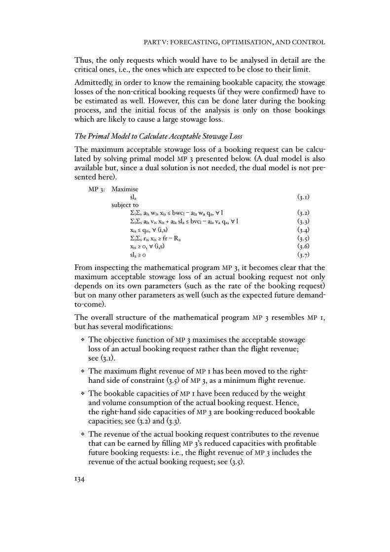
Thus, the only requests which would have to be analysed in detail are the critical ones, i.e., the ones which are expected to be close to their limit.

Admittedly, in order to know the remaining bookable capacity, the stowage losses of the non-critical booking requests (if they were confirmed) have to be estimated as well. However, this can be done later during the booking process, and the initial focus of the analysis is only on those bookings which are likely to cause a large stowage loss.

The Primal Model to Calculate Acceptable Stowage Loss

The maximum acceptable stowage loss of a booking request can be calcu-lated by solving primal model MP 3 presented below. (A dual model is also available but, since a dual solution is not needed, the dual model is not pre-sented here).

MP 3:0 Maximise0 0 sla0 0 0 0 0 0 0 0 0 (3.1)0 subject to0 0 ∑i∑s als wis xis ≤ bwcl – ala wa qa, ∀ l 00 0 0 0 (3.2)0 0 ∑i∑s als vis xis + ala sla ≤ bvcl – ala va qa, ∀ l 0 0 0 0 (3.3)0 0 xis ≤ qis, ∀ (i,s)0 0 0 0 0 0 0 (3.4)0 0 ∑i∑s ris xis ≥ fr – Ra0 0 0 0 0 0 0 (3.5)0 0 xis ≥ 0, ∀ (i,s)0 0 0 0 0 0 0 0 (3.6)0 0 sla ≥ 00 0 0 0 0 0 0 0 0 (3.7)

From inspecting the mathematical program MP 3, it becomes clear that the maximum acceptable stowage loss of an actual booking request not only depends on its own parameters (such as the rate of the booking request) but on many other parameters as well (such as the expected future demand-to-come).

The overall structure of the mathematical program MP 3 resembles MP 1, but has several modifications:

❖ The objective function of MP 3 maximises the acceptable stowage loss of an actual booking request rather than the flight revenue; see (3.1).

❖ The maximum flight revenue of MP 1 has been moved to the right-hand side of constraint (3.5) of MP 3, as a minimum flight revenue.

❖ The bookable capacities of MP 1 have been reduced by the weight and volume consumption of the actual booking request. Hence, the right-hand side capacities of MP 3 are booking-reduced bookable capacities; see (3.2) and (3.3).

❖ The revenue of the actual booking request contributes to the revenue that can be earned by filling MP 3’s reduced capacities with profitable future booking requests: i.e., the flight revenue of MP 3 includes the revenue of the actual booking request; see (3.5).


134

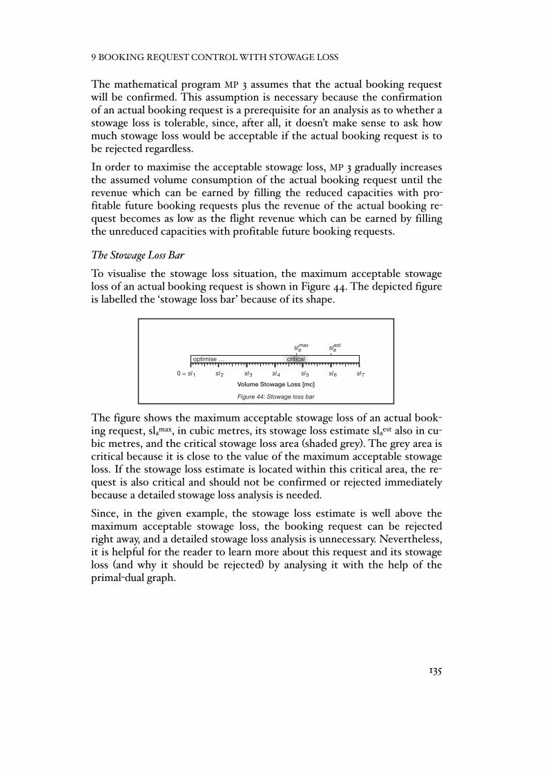
The mathematical program MP 3 assumes that the actual booking request will be confirmed. This assumption is necessary because the confirmation of an actual booking request is a prerequisite for an analysis as to whether a stowage loss is tolerable, since, after all, it doesn’t make sense to ask how much stowage loss would be acceptable if the actual booking request is to be rejected regardless.

In order to maximise the acceptable stowage loss, MP 3 gradually increases the assumed volume consumption of the actual booking request until the revenue which can be earned by filling the reduced capacities with pro-fitable future booking requests plus the revenue of the actual booking re-quest becomes as low as the flight revenue which can be earned by filling the unreduced capacities with profitable future booking requests.

The Stowage Loss Bar

To visualise the stowage loss situation, the maximum acceptable stowage loss of an actual booking request is shown in Figure 44. The depicted figure is labelled the ‘stowage loss bar’ because of its shape.

The figure shows the maximum acceptable stowage loss of an actual book-ing request, slamax, in cubic metres, its stowage loss estimate slaest also in cu-bic metres, and the critical stowage loss area (shaded grey). The grey area is critical because it is close to the value of the maximum acceptable stowage loss. If the stowage loss estimate is located within this critical area, the re-quest is also critical and should not be confirmed or rejected immediately because a detailed stowage loss analysis is needed.

Since, in the given example, the stowage loss estimate is well above the maximum acceptable stowage loss, the booking request can be rejected right away, and a detailed stowage loss analysis is unnecessary. Nevertheless, it is helpful for the reader to learn more about this request and its stowage loss (and why it should be rejected) by analysing it with the help of the primal-dual graph.

estsla

estslaamaxsl

critical

qslqsl

dsl

v sl

wsl


stowage loss*

Den

sity

Mix

of T

wo

Item

s [%

]

Uni

fied

Den

sity

Lab

els

0 1 32 54

7.2 6 void

void6

12 9! 36 18

200

166

133

100

Density [mc/t]

Density [mc/t]


–1 –.833 –.5–.66 –.166–.33 0 void


!"


Varia

ble

density withstowage

loss*

revenue

weight

revenue

effectivedemand*


volume withstowage

loss*

weight

revenue


stowage loss*

effectivedemand*

effectiverate*

rasl

–>



Varia

ble

wc[kg/chkg]

tc[kg/t]

chtc[chkg/cht]

tc[kg/t]

tc[kg/t]

tc[kg/t]


ds[mc/t]

vc[mc/cht]

ds[mc/t]

chtc[chkg/cht]

chtc[chkg/cht]

chtc[chkg/cht]

–> derivedinitial



–> derivedinitial


Varia

ble

revenue[euro]

revenue[euro]


volume*[mc]

volume*[mc]

weight[kg]

revenue[euro]



rate*[euro/chkg]


density*[mc/t]

weight[kg]

–> derivedinitial


Properties

Varia

ble

revenue[€]

revenue[€]


volume[mc]

volume[mc]

weight[kg]

revenue[€]

weightcoefficient

[chkg/chkg]


rate[€/chkg]

volumecoefficient

[chkg/chkg]

density[mc/t]

weight[kg]

0 1 32 54 7.2

scaled density

6 129 !3618

0 1 32 54 7

range split: “0 – 6” and “6 – 12”

6 98 121110

w0 w1 w3w2 w5w4 v5


6 v3v4 v0v1v2

0 1 32 54 v5


6 v3v4 v0v1v2

0 1 32 54 – 5


6 – 3– 4 – 0– 1– 2




optimise …


7sl6sl5sl4sl3sl2sl


rejectconfirm

fp mpbc


7sl6sl5sl4sl3sl2sl


fp mpbc

Sto

wag

e Lo

ss R

ange

s

sdc

0 = 1sl0 = 1sl

sdc

aa

a

a

a

amaxsl estsla


135

9.4 Stowage Loss and the Primal-Dual Graph

The purpose of showing the stowage loss of an actual booking request in a primal-dual graph is twofold. On a general level, the primal-dual graph visu-alises the requirements for obtaining capacity access and, on a more de-tailed level, the primal-dual graph shows the primal-dual mode combina-tions which do not call for an a priori check on the maximum acceptable stowage loss.

The Primal-Dual Graph with Stowage Loss

To give an example of a primal-dual graph with stowage loss, the booking request that has been displayed above in Figure 44 is shown again in Figure 45 below.

Initially, the rate ra of the actual booking request is located in the area which is definitely profitable (i.e., in dual mode 1), while the demand qa is located in the area which is feasible (i.e., in primal mode 2). Then, due to the stowage loss, the effective rate rasl moves into the profitable area (i.e., to dual mode 2). This mode change is dubbed fp, since the rate with stow-age loss (i.e., the effective rate) crosses the full segment price line fps. From there on, any further stowage loss moves the effective demand qasl towards

s

bwcs

bvcs

mpsmvps

fpsfvps

fwps

fcsfvcs

fwcs bc

estsl

estsl

XXI

10 = cw

2cw

3cw

4cw

5cw

6cw

7cw

8cw

9 cw

00 2 4 96 !18

Density [mc/t]

Cha

rgea

ble

Wei

ght [

cht]


Rat

e [€

/chk

g]

9r

8r

7r

6r

5r

4r

3r

2r

1 0 = r


lowdemand

highdemand

profitable

not profitable

not feasible

feasible

defin

itely

feas

ible



Flig

ht R

even

ue [e

uro]



9rf

8rf

7rf

6rf

5rf

4rf

3rf

2rf

1 0 = rf



FractionalPerfect


Flig

ht R

even

ue [e

uro]



9rf

8rf

7rf

6rf

5rf

4rf

3rf

2rf

1 0 = rf


3 km…p4 km…p

5 km…p6 km…p

7

Sto

wag

e Lo

ss R

ange

sFl

ight

Rev

enue

[eur

o]



9rf

8rf

7rf

6rf

5rf

4rf

3rf

2rf

1


nolo

ss

Rev

enue

Pot

entia

l

Rev

enue

Pot

entia

lye

sga

inFirst ComeFirst Serve

FractionalPerfect

Hindsight


10 = cw

2cw

3cw

4cw

5cw

6cw

7cw

8cw

9 cw

00 2 4 96 !18

Density [mc/t]

Cha

rgea

ble

Wei

ght [

cht]


Rat

e [€

/chk

g]

9r

8r

7r

6r

5r

4r

3r

2r

1 0 = r


profitable

not profitable

not feasible

feasible

defin

itely

feas

ible


qsl

optimise


fc

optimise

rejectconfirm

fp mpbc


7sl6sl5sl4sl3sl2sl

reject

mp

0 = rf

rActual Booking

Request

maxsl

maxsl

rejectconfirm

mpbc

reject

fp

0 = 1sl

sdc

bc

fp

mp

sdc

fp

mp

bc

ss

s

bwcs

bvcs

mps

mwpsmwps

mvps

fpsfvps

fwps

fcsfvcs

fwcs bc

ar

aq

a

aa

aaq

a

rsla


136

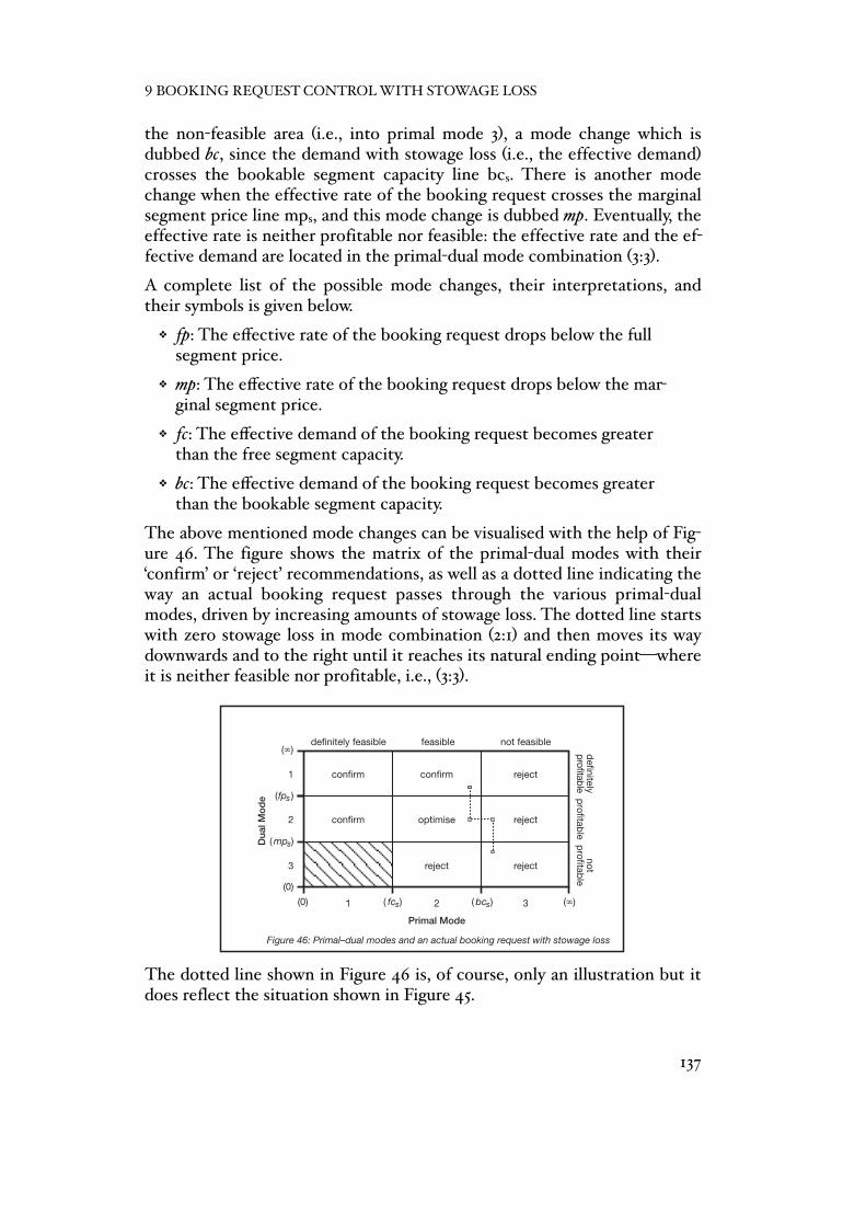
the non-feasible area (i.e., into primal mode 3), a mode change which is dubbed bc, since the demand with stowage loss (i.e., the effective demand) crosses the bookable segment capacity line bcs. There is another mode change when the effective rate of the booking request crosses the marginal segment price line mps, and this mode change is dubbed mp. Eventually, the effective rate is neither profitable nor feasible: the effective rate and the ef-fective demand are located in the primal-dual mode combination (3:3).

A complete list of the possible mode changes, their interpretations, and their symbols is given below.

❖ fp: The effective rate of the booking request drops below the fullsegment price.

❖ mp: The effective rate of the booking request drops below the mar-ginal segment price.

❖ fc: The effective demand of the booking request becomes greater than the free segment capacity.

❖ bc: The effective demand of the booking request becomes greaterthan the bookable segment capacity.

The above mentioned mode changes can be visualised with the help of Fig-ure 46. The figure shows the matrix of the primal-dual modes with their ‘confirm’ or ‘reject’ recommendations, as well as a dotted line indicating the way an actual booking request passes through the various primal-dual modes, driven by increasing amounts of stowage loss. The dotted line starts with zero stowage loss in mode combination (2:1) and then moves its way downwards and to the right until it reaches its natural ending point—where it is neither feasible nor profitable, i.e., (3:3).

The dotted line shown in Figure 46 is, of course, only an illustration but it does reflect the situation shown in Figure 45.

( )smp

( )sfp

s( )fc s( )bc

!

VI

reject

reject

reject

Figure 39: Primal–dual modes and an actual booking request

Primal Mode

Dua

l Mod

e

1 2 3

reject

confirm

optimise

1

2

3



confirm

confirm

optimise

Confirmation of a booking request. Case 3: fcs = 0, bps = 0


Pric

e [e

uro/

chkg

]

no

yesno

no

no

0fcs 0acs

0

bps 0

aps

yes

yes

not possible

optimise

Confirmation of a booking request. Case 1: fcs > 0, bps = 0


Pric

e [e

uro/

chkg

]

no

yesno

no

no

0fcsacs

0

bps 0

aps

yes

yes

not possible

0

optimise

Confirmation of a booking request. Case 2: bps > 0, fcs = 0


Pric

e [e

uro/

chkg

]

no

yesno

no

no

fcs 0acs

bps

aps

yes

yes

not possible

0

Size, rate and the confirmation of a booking request


Pric

e [e

uro/

chkg

]

0fcsacs

0

bps

aps

0 2 4 96 18

4.00

3.50

3.00

2.50

2.00

0.50

1.50

1.00

0.00

Density [mc/t]

Pric

e [e

uro/

chkg

]

Volume Stowage Loss, Rate and Density

! 0 2 4 96 18

0

1

2

3

4

7

5

6

8

Density [mc/t]

Cha

rgea

ble

Wei

ght [

cht]

Volume Stowage Loss, Demand and Density

300

200

100d

D = f (d )slsl

max dsl

0 10080604020 0 10080604020

d

r = f (d )slsl

max dsl

Volume S

towage Loss [%

]

300

200

100

Volume S

towage Loss [%

]

(!)(0)

(0)

(!)

reject

reject

reject

Figure 46: Primal–dual modes and an actual booking request with stowage loss

Primal Mode

Dua

l Mod

e

1 2 3

reject

confirm

optimise

1

2

3

confirm

confirm

(!)(0)

(0)

(!)

( )smp

( )sfp

s( )fc s( )bc

notprofitable


notprofitable



137

Rejection of the actual booking request is still recommended because of the estimated stowage loss. However, this time, the recommendation is not based on a separate calculation of the maximum acceptable stowage loss of the booking request but on the fact that, due to the estimated stowage loss, the actual booking request, while still profitable, is no longer feasible. Hence, when the primal-dual mode combination of the actual booking re-quest with its estimated stowage loss is (3:2), the recommendation is to ‘reject’.

The Stowage Loss Bar with Primal-Dual Modes

The primal and dual modes can also be used to enhance the stowage loss bar of an actual booking request. If the stowage loss bar also shows the primal and dual modes, the bar contains all the major information con-tained within the primal-dual graph. An example of a stowage loss bar with primal and dual modes is shown in Figure 47.

The upper part of the figure shows a stowage loss bar complete with an optimisation range, and the lower part shows the same stowage loss bar but with a maximum acceptable stowage loss. The maximum acceptable stow-age loss was calculated separately but, from what was said earlier, it is clear that, for the given booking request, a calculation of the maximum accept-able stowage loss was unnecessary. Calculating slamax is only necessary if the stowage loss is likely to fall within the optimisation range.

In addition to the optimisation range and the maximum acceptable stow-age loss, the primal and dual modes of the actual booking request are indicated for various amounts of stowage loss. However, the primal and dual modes are not shown explicitly but rather implied. In other words, whenever an actual booking request changes its primal or dual mode due to stowage loss, the respective value and a description of the mode change are registered and displayed. Halfway between sl3 and sl4, for example, the actual booking request changes its dual mode from ‘definitely profitable’ to ‘profitable’. This value is displayed in the stowage loss bar and marked as fp.

estslaamaxsl

critical

qslqsl

dsl

v sl

wsl


stowage loss*

Den

sity

Mix

of T

wo

Item

s [%

]

Uni

fied

Den

sity

Lab

els

0 1 32 54

7.2 6 void

void6

12 9! 36 18

200

166

133

100

Density [mc/t]

Density [mc/t]


–1 –.833 –.5–.66 –.166–.33 0 void


!"


Varia

ble

density withstowage

loss*

revenue

weight

revenue

effectivedemand*


volume withstowage

loss*

weight

revenue


stowage loss*

effectivedemand*

effectiverate*

rasl

–>



Varia

ble

wc[kg/chkg]

tc[kg/t]

chtc[chkg/cht]

tc[kg/t]

tc[kg/t]

tc[kg/t]


ds[mc/t]

vc[mc/cht]

ds[mc/t]

chtc[chkg/cht]

chtc[chkg/cht]

chtc[chkg/cht]

–> derivedinitial



–> derivedinitial


Varia

ble

revenue[euro]

revenue[euro]


volume*[mc]

volume*[mc]

weight[kg]

revenue[euro]



rate*[euro/chkg]


density*[mc/t]

weight[kg]

–> derivedinitial


Properties

Varia

ble

revenue[€]

revenue[€]


volume[mc]

volume[mc]

weight[kg]

revenue[€]

weightcoefficient

[chkg/chkg]


rate[€/chkg]

volumecoefficient

[chkg/chkg]

density[mc/t]

weight[kg]

0 1 32 54 7.2

scaled density

6 129 !3618

0 1 32 54 7

range split: “0 – 6” and “6 – 12”

6 98 121110

w0 w1 w3w2 w5w4 v5


6 v3v4 v0v1v2

0 1 32 54 v5


6 v3v4 v0v1v2

0 1 32 54 – 5


6 – 3– 4 – 0– 1– 2




optimise …


7sl6sl5sl4sl3sl2sl


rejectconfirm

fp mpbc


7sl6sl5sl4sl3sl2sl

Sto

wag

e Lo

ss R

ange

s

sdc

0 = 1sl0 = 1sl

aa

a

a

a

amaxsl estsla

estsla


fp mpbcsdc


138

Figure 47 also shows the value at which the booking request’s density with stowage loss becomes equal to the standard density (‘sdc’). This value is im-portant because it denotes the amount of stowage loss from where on the effective demand begins to increase which, in turn, implies that the effec-tive rate must decrease.

Note that any stowage loss that results in the density with stowage loss be-ing less than the standard density will neither change the demand of the booking request, nor its rate. Hence, even if the customer has agreed to compensate for any lower effective rate, there will be no need to do so since the effective rate has not changed.

The critical stowage loss area is shown in both parts of Figure 47. The criti-cal stowage loss area was earlier dubbed ‘critical’ because of its proximity to the value of the maximum acceptable stowage loss. Essentially, the area is critical because it is in this area where a small increase in the amount of stowage loss may reverse the recommendation to confirm an actual book-ing request. For this reason, the critical stowage loss area in the upper stowage loss bar has been split to reflect the situation that to the left of the optimisation range, the recommendation to confirm an actual booking re-quest can easily change into one to reject it, and to the right of the optimi-sation range, the recommendation to reject an actual booking request can easily change into one to confirm it—depending on the accuracy of the stowage loss estimate and the maximum acceptable stowage loss.

Finally, the differences between a stowage loss bar and a primal-dual graph will be assessed:

❖ The stowage loss bar has fewer dimensions (i.e., one dimension rather than three).

❖ The stowage loss bar shows the consequences of an increasing volume, whereas the primal-dual graph shows the consequences of a decreasing density. In other words, the bar is closer to the roots of stowage loss, whereas the primal-dual graph argues through an intermediary variable.

❖ The stowage loss bar shows the economic reasoning behind a primal-dual graph in a technical context of cubic metres. Since the stowage loss is estimated in cubic metres, it makes sense to also analyse its economic consequences in cubic metres.

With regard to the decision as to whether to confirm or reject an actual booking request, however, both figures, the stowage loss bar and the primal-dual graph, are equivalents.


139

The Renegotiation of Stowage Loss

The main purpose of the primal-dual graph with stowage loss and the stow-age loss bar display is to support renegotiations with the customer if it is foreseen that an actual booking request will cause a considerable stowage loss. For this purpose, it is not even necessary for the estimated stowage loss to be greater than the maximum acceptable stowage loss; renegotia-tions can begin when the estimated density with stowage loss is higher than the standard density. Or, to put it differently, when the effective demand of the booking request with stowage loss is higher than the original demand without stowage loss.

There now follows a further discussion that serves as an example of how the stowage loss bar can be used to renegotiate the terms of a booking request with the customer. In the given example, referring to the figures above, the recommendation was to reject the booking request because of its stowage loss. However, by looking at the upper stowage loss bar in Figure 47, it can be seen that the stowage loss of the booking request (as it has thus far been estimated) is simply too great to fit into the bookable ca-pacity. Hence, either a way has to be found to increase the bookable vol-ume capacity on the requested segment, or the volume stowage loss itself has to be brought down.

However, not only is the capacity a problem, the rate is as well (as can be seen from the fact that the maximum acceptable stowage loss slamax, shown in the lower stowage loss bar of Figure 47, is lower than the bookable ca-pacity). This situation has arisen because, while the original rate is com-paratively high (it is well above the full segment price), the effective rate of the booking request with stowage loss is comparatively low (it is close to the marginal segment price). To further clarify the issue, the fact that the original rate is comparatively high can be seen by the distance between the zero reference point sl1 and fp, and the fact that the effective rate is com-paratively low can be seen from the distance between the stowage loss esti-mate slaest and mp.

Hence, potential solutions are to increase the chargeable weight of the booking request to the ‘real’ chargeable weight with stowage loss, which will retain the booking request’s original rate, or increase the rate. This is possible (and attractive) because the estimated stowage loss (see slaest at sl6 in Figure 47) is well to the right of the stowage loss that indicates the book-ing request’s standard density (see sdc at sl4).

Such a solution is, of course, subject to the customer’s agreement but, as Pak wrote, “it is no exception that the price for a potential cargo shipment is subject to negotiation before the actual booking request is made” (Pak 2005, page 114), and so higher chargeable weights or higher rates might be an option.


140

To illustrate the concept further, Figure 48 presents the stowage loss bars of four other booking requests. The first stowage loss bar shows a high-density booking request with a favourable rate. However, the booking re-quest is—even without stowage loss—too large to fit into the bookable ca-pacity and should therefore be rejected. It is possible to have a confirma-tion range and a rejection range, but no intermediate optimisation range. The second stowage loss bar, for example, has no optimisation range be-cause, for this booking request, the limiting factor is the bookable capacity and not the rate. In other words: the effective rate with stowage loss seems to be higher than the full price of the requested segment, even with large amounts of stowage loss.

It is important to note that not all stowage loss bars show the value sdc at which the booking request’s density with stowage loss is equal to the stan-dard density. This situation occurs if the actual booking request’s density without stowage loss is lower than the standard density since the density with stowage loss will be even lower.

The third stowage loss bar shows a high-density booking request with a low rate that is close to the marginal segment price, while the fourth stowage loss bar shows a comparatively small booking request with a comparatively high rate.

9.5 Contribution

The contribution of this chapter is the development of the primal-dual graph with stowage loss and its one-dimensional companion, the stowage loss bar. The analysis of the relationship between the stowage loss of a booking request and the instruments available to increase the revenue of a flight is also considered an important contribution.

s

bwcs

bvcs

mpsmvps

fpsfvps

fwps

fcsfvcs

fwcs bc

estsl

estsl

XXI

10 = cw

2cw

3cw

4cw

5cw

6cw

7cw

8cw

9 cw

00 2 4 96 !18

Density [mc/t]

Cha

rgea

ble

Wei

ght [

cht]


Rat

e [€

/chk

g]

9r

8r

7r

6r

5r

4r

3r

2r

1 0 = r


lowdemand

highdemand

profitable

not profitable

not feasible

feasible

defin

itely

feas

ible



Flig

ht R

even

ue [e

uro]



9rf

8rf

7rf

6rf

5rf

4rf

3rf

2rf

1 0 = rf



FractionalPerfect


Flig

ht R

even

ue [e

uro]



9rf

8rf

7rf

6rf

5rf

4rf

3rf

2rf

1 0 = rf


3 km…p4 km…p

5 km…p6 km…p

7

Sto

wag

e Lo

ss R

ange

sFl

ight

Rev

enue

[eur

o]



9rf

8rf

7rf

6rf

5rf

4rf

3rf

2rf

1


nolo

ss

Rev

enue

Pot

entia

l

Rev

enue

Pot

entia

lye

sga

in


FractionalPerfect

Hindsight


10 = cw

2cw

3cw

4cw

5cw

6cw

7cw

8cw

9 cw

00 2 4 96 !18

Density [mc/t]

Cha

rgea

ble

Wei

ght [

cht]


Rat

e [€

/chk

g]

9r

8r

7r

6r

5r

4r

3r

2r

1 0 = r


profitable

not profitable

not feasible

feasible

defin

itely

feas

ible


qsl

optimise


fc

optimise

rejectconfirm

fp mpbc


7sl6sl5sl4sl3sl2sl

reject

mp

0 = rf

rActual Booking

Request

maxsl

maxsl

rejectconfirm

mpbc

reject

fp

0 = 1sl

sdc

bc

fp

mp

sdc

fp

mp

bc

ss

s

bwcs

bvcs

mps

mwpsmwps

mvps

fpsfvps

fwps

fcsfvcs

fwcs bc

ar

aq

a

aa

aaq

a

rsla


141

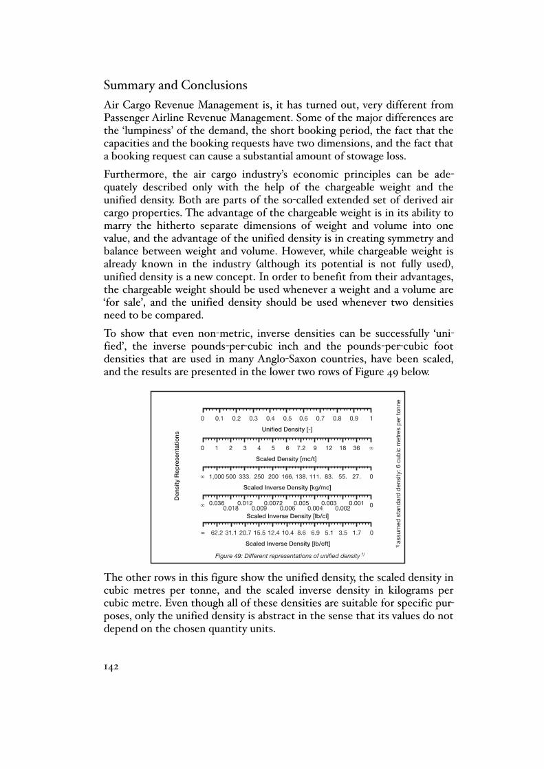
Summary and Conclusions

Air Cargo Revenue Management is, it has turned out, very different from Passenger Airline Revenue Management. Some of the major differences are the ‘lumpiness’ of the demand, the short booking period, the fact that the capacities and the booking requests have two dimensions, and the fact that a booking request can cause a substantial amount of stowage loss.

Furthermore, the air cargo industry’s economic principles can be ade-quately described only with the help of the chargeable weight and the unified density. Both are parts of the so-called extended set of derived air cargo properties. The advantage of the chargeable weight is in its ability to marry the hitherto separate dimensions of weight and volume into one value, and the advantage of the unified density is in creating symmetry and balance between weight and volume. However, while chargeable weight is already known in the industry (although its potential is not fully used), unified density is a new concept. In order to benefit from their advantages, the chargeable weight should be used whenever a weight and a volume are ‘for sale’, and the unified density should be used whenever two densities need to be compared.

To show that even non-metric, inverse densities can be successfully ‘uni-fied’, the inverse pounds-per-cubic inch and the pounds-per-cubic foot densities that are used in many Anglo-Saxon countries, have been scaled, and the results are presented in the lower two rows of Figure 49 below.

The other rows in this figure show the unified density, the scaled density in cubic metres per tonne, and the scaled inverse density in kilograms per cubic metre. Even though all of these densities are suitable for specific pur-poses, only the unified density is abstract in the sense that its values do not depend on the chosen quantity units.

Figure 49: Different representations of unified density

Den

sity

Rep

rese

ntat

ions

XVII

Scaled Inverse Density [lb/cft]

! 62.2 20.731.1 12.415.5 8.610.4 5.16.9 01.73.5

Scaled Inverse Density [kg/mc]

! 1,000 333.500 200250 138.166. 83.111. 027.55.

Scaled Inverse Density [lb/ci]

! 0.036 0.0120.018

0.00720.009

0.0050.006

0.0030.004 00.001

0.002

Unified Density [-]

0.6 0.8 0.90 0.1 0.30.2 0.50.4 10.7


0 1 32 54 7.26 129 !3618

1)

assu

med

sta

ndar

d de

nsity

: 6 c

ubic

met

res

per t

onne

1)

142

Hence, only the unified density, as with the chargeable weight, is a univer-sal economic term.

Both unified density and scaled density are used by Lufthansa Cargo, one of the largest air cargo carriers in the world, and are patent pending.

Further, of the instruments that are proposed to increase the revenue of a flight, three are of a somewhat generic nature and could also be used to manage other revenues in air transportation (including passenger revenues), while two are specific to air cargo. The generic instruments are to confirm booking requests that have favourable rates, to opt for booking requests that have short routes, and to combine booking requests that have diverse routings, while the cargo-specific instruments are to prefer booking re-quests that have a suitable density, and to mix booking requests that have high and low densities.

However, no matter what individual instruments are available, in order to use them effectively it is not only necessary to have a reliable demand fore-cast, to run an efficient revenue optimisation procedure, and to apply an appropriate booking request control; it is also necessary that the values of the demand forecast are in the right format (with regard to grid coarseness etc.) so that they can be used in revenue optimisation. Further, the values resulting from revenue optimisation have to have the right format (with regard to their quantity units etc.) so that they can be used in the booking request control.

Finally, it has been shown that calculating the lumpy bid price of a booking request is fundamental in deciding whether it should be confirmed, and that it is beneficial to calculate a range of price and capacity curves in order to be able to produce the primal-dual graph.

The decision support offered by the primal-dual graph is particularly wel-come if the decision to confirm (or to reject, for that matter) is uncertain, or if the booking request is likely to cause substantial stowage loss. In the latter case, it is also worthwhile consulting the stowage loss bar to deter-mine the correct decision.

SUMMARY AND CONCLUSIONS

143

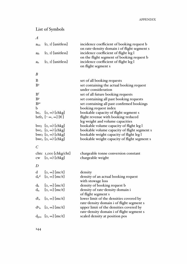
List of Symbols

A

abis0 {0, 1} [unitless]0 0 incidence coefficient of booking request b0 0 0 0 0 on rate-density domain i of flight segment salb0 {0, 1} [unitless]0 0 incidence coefficient of flight leg l0 0 0 0 0 on the flight segment of booking request bals0 {0, 1} [unitless]0 0 incidence coefficient of flight leg l0 0 0 0 0 on flight segment s

B

B0 0 0 0 0 set of all booking requestsBa0 0 0 0 0 set containing the actual booking request0 0 0 0 0 under considerationBf0 0 0 0 0 set of all future booking requestsBp0 0 0 0 0 set containing all past booking requestsBpc0 0 0 0 0 set containing all past confirmed bookingsb0 0 0 0 0 booking request indexbcs0 [0, ∞) [chkg]0 0 bookable capacity of flight segment sbrfra0 [– ∞, ∞] [€]0 0 flight revenue with booking-reduced0 0 0 0 0 leg weight and volume capacitiesbvcl0 [0, ∞) [chkg]0 0 bookable volume capacity of flight leg lbvcs0 [0, ∞) [chkg]0 0 bookable volume capacity of flight segment sbwcl0 [0, ∞) [chkg]0 0 bookable weight capacity of flight leg lbwcs0 [0, ∞) [chkg]0 0 bookable weight capacity of flight segment s

C

chtc 0 1,000 [chkg/cht]00 chargeable tonne conversion constantcw0 [0, ∞) [chkg]0 0 chargeable weight

D

d0 [0, ∞] [mc/t]0 0 densitydasl0 [0, ∞] [mc/t]0 0 density of an actual booking request 0 0 0 0 0 with stowage lossdb0 [0, ∞] [mc/t]0 0 density of booking request bdis0 [0, ∞] [mc/t]0 0 density of rate-density domain i 0 0 0 0 0 of flight segment sdlis0 [0, ∞] [mc/t]0 0 lower limit of the densities covered by 0 0 0 0 0 rate-density domain i of flight segment sduis0 [0, ∞] [mc/t]0 0 upper limit of the densities covered by 0 0 0 0 0 rate-density domain i of flight segment sdpos0 [0, ∞] [mc/t]0 0 scaled density at position pos

APPENDIX

144

E, F

fcs0 [0, ∞) [chkg]0 0 free capacity of flight segment sfps0 [0, ∞] [€/chkg]0 0 full price of flight segment sfr0 [– ∞, ∞] [€]0 0 flight revenuefvcl0 [0, ∞) [chkg]0 0 free volume capacity of flight leg lfvcs0 [0, ∞) [chkg]0 0 free volume capacity of flight segment sfwcl0 [0, ∞) [chkg]0 0 free weight capacity of flight leg lfwcs0 [0, ∞) [chkg]0 0 free weight capacity of flight segment s

G, H, I

i0 0 0 0 0 rate-density domain index

J, K, L

l0 0 0 0 0 flight leg indexlpa0 [0, ∞] [€/chkg]0 0 lumpy price of an actual booking request

M

mpa0 [0, ∞] [€/chkg]0 0 marginal price of an actual booking requestmvpl0 [0, ∞] [€/chkg]0 0 marginal price of volume capacity of flight leg lmvps0[0, ∞] [€/chkg]0 0 marginal volume price of flight segment smwpl0[0, ∞] [€/chkg]0 0 marginal price of weight capacity of flight leg lmwps0[0, ∞] [€/chkg]0 0 marginal weight price of flight segment sµbis0 [0, 1] [unitless]0 0 booking request b’s share of the aggregated 0 0 0 0 0 demand-to-come of domain i of flight 0 0 0 0 0 segment s

N, O, P

p0 [unitless]0 0 0 number of positionspis0 [0, ∞) [€/chkg]0 0 profitability of rate-density domain i 0 0 0 0 0 of flight segment spos0 0 0 0 0 position index

Q

qasl0 (0, ∞) [chkg]0 0 demand (quantity) of an actual booking request0 0 0 0 0 with stowage loss; also called effective demandqb0 (0, ∞) [chkg]0 0 demand (quantity) of booking request bqis0 [0, ∞) [chkg]0 0 demand-to-come of rate-density domain i 0 0 0 0 0 of flight segment sqs0 [0, ∞) [chkg]0 0 demand-to-come for flight segment s

LIST OF SYMBOLS

145

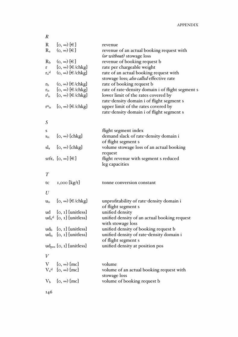
R

R0 [0, ∞) [€]0 0 0 revenueRa0 (0, ∞) [€]0 0 0 revenue of an actual booking request with0 0 0 0 0 (or without) stowage lossRb0 (0, ∞) [€]0 0 0 revenue of booking request br0 [0, ∞) [€/chkg]0 0 rate per chargeable weightrasl0 (0, ∞) [€/chkg]0 0 rate of an actual booking request with 0 0 0 0 0 stowage loss; also called effective raterb0 (0, ∞) [€/chkg]0 0 rate of booking request bris0 [0, ∞) [€/chkg]0 0 rate of rate-density domain i of flight segment srlis0 [0, ∞) [€/chkg]0 0 lower limit of the rates covered by 0 0 0 0 0 rate-density domain i of flight segment sruis0 [0, ∞) [€/chkg]0 0 upper limit of the rates covered by 0 0 0 0 0 rate-density domain i of flight segment s

S

s0 0 0 0 0 flight segment indexsis0 [0, ∞) [chkg]0 0 demand slack of rate-density domain i 0 0 0 0 0 of flight segment ssla0 [0, ∞) [chkg]0 0 volume stowage loss of an actual booking 0 0 0 0 0 requestsrfrs0 [0, ∞] [€]0 0 0 flight revenue with segment s reduced 0 0 0 0 0 leg capacities

T

tc0 1,000 [kg/t]0 0 tonne conversion constant

U

uis0 [0, ∞) [€/chkg]0 0 unprofitability of rate-density domain i 0 0 0 0 0 of flight segment sud0 [0, 1] [unitless]0 0 unified densityudasl0 [0, 1] [unitless]0 0 unified density of an actual booking request 0 0 0 0 0 with stowage lossudb0 [0, 1] [unitless]0 0 unified density of booking request budis0 [0, 1] [unitless]0 0 unified density of rate-density domain i 0 0 0 0 0 of flight segment sudpos0 [0, 1] [unitless]0 0 unified density at position pos

V

V0 [0, ∞) [mc]00 0 volumeVasl0 [0, ∞) [mc]00 0 volume of an actual booking request with 0 0 0 0 0 stowage lossVb0 [0, ∞) [mc]00 0 volume of booking request b

APPENDIX

146

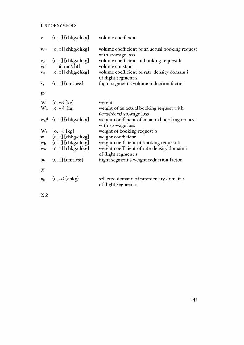
v0 [0, 1] [chkg/chkg]0 volume coefficient

vasl0 [0, 1] [chkg/chkg]0 volume coefficient of an actual booking request0 0 0 0 0 with stowage lossvb0 [0, 1] [chkg/chkg]0 volume coefficient of booking request bvc0 6 [mc/cht]0 0 volume constantvis0 [0, 1] [chkg/chkg]0 volume coefficient of rate-density domain i 0 0 0 0 0 of flight segment sνs0 [0, 1] [unitless]0 0 flight segment s volume reduction factor

W&

W0 [0, ∞) [kg]0 0 0 weightWa0 [0, ∞) [kg]0 0 0 weight of an actual booking request with0 0 0 0 0 (or without) stowage losswasl0 [0, 1] [chkg/chkg]0 weight coefficient of an actual booking request0 0 0 0 0 with stowage lossWb0 [0, ∞) [kg]0 0 0 weight of booking request bw0 [0, 1] [chkg/chkg]0 weight coefficientwb0 [0, 1] [chkg/chkg]0 weight coefficient of booking request bwis0 [0, 1] [chkg/chkg]0 weight coefficient of rate-density domain i 0 0 0 0 0 of flight segment sωs0 [0, 1] [unitless]0 0 flight segment s weight reduction factor

X

xis0 [0, ∞) [chkg]0 0 selected demand of rate-density domain i 0 0 0 0 0 of flight segment s

Y, Z

LIST OF SYMBOLS

147

List of Mathematical Programs, Figures, and Tables

Mathematical Programs

10 Primal model to calculate the flight revenue 20 Dual model to calculate the flight revenue 30 Primal model to calculate the acceptable stowage loss 0 of a booking request

Figures

10 Air Transportation involving one (or several) flight(s) 20 Weight, volume, and density 30 Weight, volume, and chargeable weight 40 Density, standard density, and chargeable weight 50 Simple set of derived air cargo properties 60 Extended set of derived air cargo properties 70 Extended set of derived air cargo properties, adapted to costs 80 Flight with two legs and three segments 90 Booking process

100 Minimum revenue and chargeable weight breakpoints 11 0 Specific weight and volume consumption of high-density freight 120 Specific weight and volume consumption of low-density freight 130 Unified density of low-density freight 140 Unified density and scaled density 150 Construction and legend of the density scaling 160 Various scaled densities with an even number of positions 170 Various scaled densities with an odd number of positions 180 Various labels for unified density 190 Density, standard density, and unified density

200 Various densities and the extended set 210 Rate-density distribution of real-world demand 220 Rate-graph of a segment 230 Density-graph of a segment 240 Weight and volume consumption-graph of a segment 250 Booking requests, a rate-density domain, and its gravity centre 260 Comparison of two different rate-density grid setups 270 Generic rate-density grid 280 Legend of some of the primal parameters and variables 290 Primal graph with various free volume capacities

APPENDIX

148

300 Primal graph with various free weight capacities 310 Legend of some of the dual parameters and variables 320 Dual graph with various marginal volume prices 330 Dual graph with various marginal weight prices 340 Rate-density domains, gravity centres, 0 and the marginal segment price 350 Free and bookable segment capacities, and the primal modes 360 Marginal and full segment prices, and the dual modes 370 Primal-dual graph with an unprofitable booking request 380 Primal-dual graph with a definitely profitable booking request 390 Primal-dual modes and an actual booking request

400 Primal-dual graph for a volume-restricted flight segment 410 Propagation of stowage loss 420 Three booking requests and their rate decrease due to stowage loss 430 Three booking requests and their demand increase 0 due to stowage loss 440 Stowage loss bar 450 Primal-dual graph with a booking request and stowage loss 460 Primal-dual modes and an actual booking request with stowage loss 470 Stowage loss ranges for an actual booking request 480 Various booking requests and their stowage loss range 490 Different representations of unified density

Tables

10 Weight and volume consumption I 20 Weight and volume consumption II 30 The effects of 1.8 [mc] stowage loss on three booking requests

LIST OF MATHEMATHICAL PROGRAMS, FIGURES, AND TABLES

149

Bibliography

ACCC:Detailed Analysis of IATA Resolution 502 (Low Density Cargo) Volumetric Ratio /by the Australian Competition and Consumer Commission.Sydney: ACCC, 2004.URL: http://www.accc.gov.au/content/trimFile.phtml?trimFileName=D04+42224.pdf&trimFileTitle=D04+42224.pdf&trimFileFromItemId=503770

Air Cargo World:October Issue /by Air Cargo World.Washington: Commonwealth Business Media, 1996.

Bartodziej, Paul and Ulrich Derigs:On an Experimental Algorithm for Revenue Management for Cargo Airlines /by Paul Bartodziej and Ulrich Derigs.In: Lecture Notes in Computer Science, 3059, pages 57-71. 2004.

Bazaraa, Mokhtar et al.:The Asia Pacific Air Cargo System /by Mokhtar Bazaraa, Joseph D. Hurley, Ellis L. Johnson,George L. Nemhauser, Joel S. Sokol, I-Lin Wang,Ek-Peng Chew, Huei Chuen Huang, Ivy Mok, Kok ChoonTan and Chung Piaw Teo.Singapore: TLI-AP, 2001.In: Engineering Research News, 18-2, pages 3ff., 2003.

Billings, John S. et al.:Cargo Revenue Optimisation /by John S. Billings, Adriana G. Diener and Benson B. Yuen.In: Journal of Revenue and Pricing Management, 2, pages 69-79. 2003.

Blomeyer, Johannes:Capacity and Revenue Management /by Johannes Blomeyer.Working Paper (Unpublished)Frankfurt: Lufthansa Cargo AG, 1999.

Blomeyer, Johannes:System und Verfahren zur Optimierung der Auslastungeines Frachtraums und zur Maximierung des Erlöses füreinen Frachttransport /by Johannes Blomeyer.

APPENDIX

150

German Patent- and Trademark Office DE 10 2004 023 833,European Patent Office EP 1 596 317 A1, and United States Patent- and Trademark Office US 2006 001 5396 A1.Frankfurt: Lufthansa Cargo AG, 2004.

Boer, Sanne V. de et al.:Stochastic Programming for Multiple Leg Network Revenue Management /by Sanne V. de Boer, Richard Freling and Nanda Piersma.Gouda: Ortec, 1999.URL: http://www.eur.nl/Webdoc/doc/econometrie/feweco19990907115746.pdf

Boyd, Andrew E. and Ioana C. Bilegan:Revenue Management and e-Commerce /by Andrew E. Boyd and Ioana C. Bilegan.Houston: Pros, 2003.URL: http://www.prosrm.com/files/ms%20paper%20v6.pdf

Butler, Gail F. and Martin R. Keller:Handbook of Airline Marketing /edited by Gail F. Butler and Martin R. Keller.New York: McGraw-Hill, 1998.

Butler, Gail F. and Martin R. Keller:Handbook of Airline Finance /edited by Gail F. Butler and Martin R. Keller.New York: McGraw-Hill, 1999.

Cakanyildirim, Metin and Lama Moussawi:Profit Maximization in Air Cargo Overbooking /by Metin Cakanyildirim and Lama Moussawi.Dallas: University of Texas at Dallas, 2005.URL: http://som.utdallas.edu/faculty/working_papers/som200562.pdf

Chen, Victoria C.P. et al.:Routing Considerations in Airline Yield Management /by Victoria C.P. Chen, Dirk Günther and Ellis L. Johnson.Arlington: University of Texas, 2003.URL: http://www.ie.uta.edu/researchfiles/VictoriaChen_1945/orchapChen.pdf

Chew, Ek-Peng et al.:Short-Term Booking of Air Cargo Space /by Ek-Peng Chew, Huei-Chuen Huang, Ellis L. Johnson, George L. Nemhauser, Joe Sokol and Chun-How Leong.Atlanta: Georgia Institute of Technology, 2002.

BIBLIOGRAPHY

151

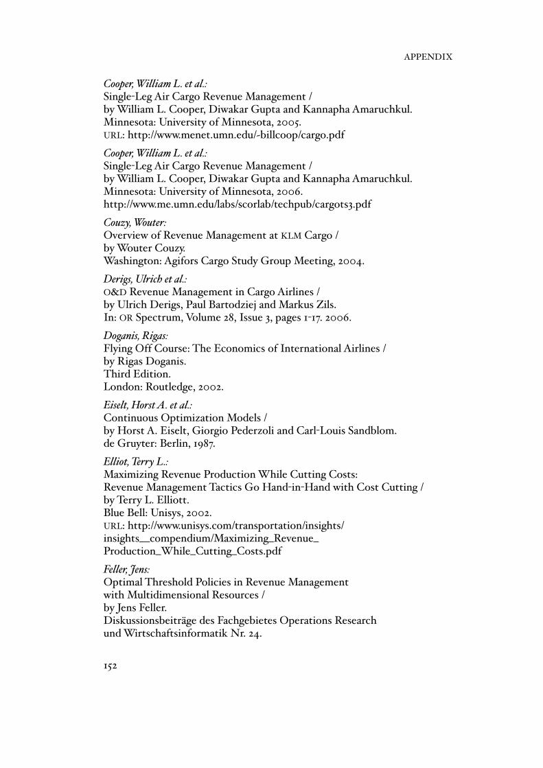
Cooper, William L. et al.:Single-Leg Air Cargo Revenue Management /by William L. Cooper, Diwakar Gupta and Kannapha Amaruchkul.Minnesota: University of Minnesota, 2005.URL: http://www.menet.umn.edu/~billcoop/cargo.pdf

Cooper, William L. et al.:Single-Leg Air Cargo Revenue Management /by William L. Cooper, Diwakar Gupta and Kannapha Amaruchkul.Minnesota: University of Minnesota, 2006.http://www.me.umn.edu/labs/scorlab/techpub/cargots3.pdf

Couzy, Wouter:Overview of Revenue Management at KLM Cargo /by Wouter Couzy. Washington: Agifors Cargo Study Group Meeting, 2004.

Derigs, Ulrich et al.:O&D Revenue Management in Cargo Airlines /by Ulrich Derigs, Paul Bartodziej and Markus Zils.In: OR Spectrum, Volume 28, Issue 3, pages 1-17. 2006.

Doganis, Rigas:Flying Off Course: The Economics of International Airlines /by Rigas Doganis.Third Edition.London: Routledge, 2002.

Eiselt, Horst A. et al.:Continuous Optimization Models /by Horst A. Eiselt, Giorgio Pederzoli and Carl-Louis Sandblom.de Gruyter: Berlin, 1987.

Elliot, Terry L.:Maximizing Revenue Production While Cutting Costs:Revenue Management Tactics Go Hand-in-Hand with Cost Cutting /by Terry L. Elliott.Blue Bell: Unisys, 2002.URL: http://www.unisys.com/transportation/insights/insights__compendium/Maximizing_Revenue_Production_While_Cutting_Costs.pdf

Feller, Jens:Optimal Threshold Policies in Revenue Managementwith Multidimensional Resources /by Jens Feller. Diskussionsbeiträge des Fachgebietes Operations Research und Wirtschaftsinformatik Nr. 24.

APPENDIX

152

Universität Dortmund: Dortmund, 2002.URL: http://www.wiso.uni-dortmund.de/orwi/de/content/download/publikation/files/dispap24.pdf

Gallego, Guillermo and Robert Phillips:Revenue Management of Flexible Products /by Guillermo Gallego and Robert Phillips.New York, IEOR Columbia University, 2003.URL: http://www.gsb.stanford.edu/facseminars/past/04-05/oit.html

Garvett, Donald S. and Kyle J. Hilton:What Drives Airline Profits /by Donald S. Garvett and Kyle J. Hilton.In: Butler and Keller 1999, pages 181ff.

Gliozzi, Stefano and Alberto Maria Marchetti:Yield Management Method and System /by Stefano Gliozzi and Alberto Maria Marchetti.United States Patent Application Publication US 2003/0065542.Armonk: IBM, 2003a.

Gliozzi, Stefano and Alberto Maria Marchetti:A New Yield Management Approach for Continuous Multi-Variable Bookings: The Airline Cargo Case / by Stefano Gliozzi and Alberto Maria Marchetti.In: Gliozzi et al. 2003, pages 369-391. 2003b.

Gliozzi, Stefano et al.:Operations Research in Space and Air /edited by Tito A. Ciriani, Giorgio Fasano, Stefano Gliozzi and Roberto Tadei.Dordrecht: Kluwer, 2003.

Groenen, Patrick J.F. and Michel van de Velden:Multidimensional Scaling /by Patrick J.F. Groenen and Michel van de Velden.Econometric Institute Reports 2004/15.Rotterdam: Erasmus University, 2004.URL: http://ep.eur.nl/handle/1765/1274

Hamoen, F.A.M.:Combination Carriers and a Dedicated Air CargoHub-and-Spoke Network /by F.A.M. Hamoen.Miami: TIACA, 1998URL: http://www.tiaca.org/content/hamoen.asp

BIBLIOGRAPHY

153

Hendricks, Gregory L. and Terry L. Elliott:Implementing Revenue Management Techniquesin an Air Cargo Environment /by Gregory L. Hendricks and Terry L. Elliott.Blue Bell: Unisys, 2003.URL: http://www.unisys.com/transportation/insights/white__papers/papers.htm?insightsid=23715

Herrmann, N. et al.,:Pricing and Revenue Management Can ReshapeYour Competitive Position in Today’s Air Cargo Business /by N. Herrmann, M. Müller, and A. Crux. In: Butler and Keller, 1998.

Holloway, Stephen:Straight and Level: Practical Airline Economics /by Stephen Holloway.2nd edition.Hampshire: Ashgate, 2003.

Huang, Kuancheng and Wenhsiu Hsu:Revenue Management for Air Cargo Space with Supply Uncertainty /by Kuancheng Huang and Wenhsiu Hsu.In: Proceedings of the Eastern Asia Society for Transportation Studies, 5, pages 570-580. 2005.URL: http://www.easts.info/on-line/proceedings_05/570.pdf

IATA:Cargo Newsletter April 2005 /by International Air Transport Association.Geneva: IATA, 2005.URL: http://www.iata.org/nr/ContentConnector/cs2000/Siteinterface/sites/whatwedo/cargo/file/CargoNewsletterApril.pdf

IATA Composite Cargo Tariff Co-ordinating Committee:Composite Resolution 502 /by International Air Transport Association.Geneva: IATA, 2002.URL: http://www.iata.org/nr/ContentConnector/cs2000/Siteinterface/pdf/cargo/Composite_Resolution_502.pdf

IATA Interline & Revenue Management Services:IRMS News Worldwide Cargo Edition: Newsletter Number 1 (February 2003) /by International Air Transport Association.

APPENDIX

154

Geneva: IATA, 2003.URL: http://www.iata.org/nr/ContentConnector/cs2000/Siteinterface/sites/tariffs/file/CargoFeb03.pdf

IATA Press Release:Low Density Cargo March 2005 /by International Air Transport Association.Geneva: IATA, 2005.URL: http://www.afif.asn.au/pdf/news/Mar05_iataLowDensity.pdf

Ingold, Anthony et al.:Yield Management: Strategies for the Service Industries /by Anthony Ingold, Una McMahon-Beatti and Ian Yeoman. 2nd edition.London: Thomson, 2001.

Kadar, Mark and John Larew:Securing the Future of Air Cargo /by Mark Kadar and John Larew. Atlanta: Mercer, 2003.URL: http://www.mercermc.com/Perspectives/Specialty/mot_pdfs/Securing_Future.pdf

Karaesmen, Itir Z.:Three Essays on Revenue Management /by Itir Z. Karaesmen.New York: Columbia University, 2001.URL: http://www.rhsmith.umd.edu/faculty/ikaraesmen/karaesmen_thesis.pdf

Kasilingam, Raja G.:Air Cargo Revenue Management: Characteristics and Complexities /by Raja G. Kasilingam.In: European Journal of Operations Research, 96, pages 36-44. 1996.

Kasilingam, Raja G.:Logistics and Transportation: Design and Planning /by Raja G. Kasilingam.Dordrecht: Kluwer, 1998.

Kimes, Sheryl E.:A Strategic Approach to Yield Management /by Sheryl E. Kimes. In: Ingold et al. 2001, pages 3-14, 2001.

BIBLIOGRAPHY

155

Kimes, Sheryl E.:Perceived Fairness of Yield Management /by Sheryl E. Kimes. In: Cornell Hotel and Restaurant Administration Quarterly, 35, pages 22-29. 1994.

Kimms, Alf and Michael Müller-Bungart:Erlössteigernde Verkaufssteuerung durch Absatzgrenzen fürLogistikdienste mit mehreren knappen Ressourcen /by Alf Kimms and Michael Müller-Bungart.In: at–Automatisierungstechnik, Volume 52, pages 304-312. 2004.

Kimms, Alf and Robert Klein:Revenue Management im Branchenvergleich /by Alf Kimms and Robert Klein.In: Zeitschrift für Betriebswirtschaft, Ergänzungsheft 1,“Revenue Management”, pages 1-30. 2005.

Klabjan, Diego and Rivi Sandhu:Fleeting with Passenger and Cargo O-D Booking Control /by Diego Klabjan and Rivi Sandhu. Washington: Agifors Cargo Study Group Meeting, 2004.

Klabjan, Diego and Rivi Sandhu:Fleeting with Passenger and Cargo O-D Booking Control /by Diego Klabjan and Rivi Sandhu. Working Paper of the Department of Mechanical and IndustrialEngineering, University of Illinois.Urbana: UIUC, 2005.URL: https://netfiles.uiuc.edu/klabjan/www/articles/cargo_pax_fleeting.pdf

Logistics Management:How to Get the Most for Your Airfreight Dollar /by Logistics Management.Sutton: Reed Business Information, 2002.URL: http://www.manufacturing.net/lm/article/ca251064.html

McGill, Jeffrey and Garrett J. van Ryzin:Revenue Management: Research Overview and Prospects /by Jeffrey I. McGill and Garrett J. van Ryzin.In: Transportation Science Vol. 33, No. 2, pages 233-256. 1999.

Narayanan, P.R.:Archetypical Science Technique in Cargo Systems /by P.R. Narayanan.Washington: Agifors Cargo Study Group Meeting, 2004.

APPENDIX

156

O’Connor, William E.:An Introduction to Airline Economics /by William E. O’Connor.6th edition.London: Praeger, 2001.

Pak, Kevin:Revenue Management:New Features and Models /by Kevin Pak. ERIM Ph.D. Series Research in Management, 61.Rotterdam: Erasmus University, 2005.URL: http://hdl.handle.net/1765/6771

Pak, Kevin and Rommert Dekker:Cargo Revenue Management:Bid-Prices for a 0–1 Multi Knapsack Problem /by Kevin Pak and Rommert Dekker. Econometric Institute Reports 2004/26.Rotterdam: Erasmus University, 2004.URL: http://hdl.handle.net/1765/1475

Popescu, Ioana:Revenue Management in a Dynamic Network Environment /by Ioana Popescu.Cambridge: Massachusetts Institute of Technology, 1999.URL: http://faculty.insead.edu/popescu/ioana/Papers/ymfinal.pdf

Radnoti, George:Profit Strategies for Air Transportation /by George Radnoti.New York: Mc Graw-Hill, 2002.

Roskam, Jan:Airplane Design: Layout Design of Cockpit, Fuselage,Wing and Empennage /by Jan Roskam.Lawrence: DARcorporation, 1989.

Sabre, Inc.:Cargo Revenue Management /by Sabre, Inc.Dallas: Sabre, 2004.URL: http://www.sabreairlinesolutions.com/products/operation/pdfs/CargoRevMgmt.pdf

BIBLIOGRAPHY

157

Silvestrini, Narciso and Ernst Peter Fischer:Color Systems in Art und Science /by Narciso Silvestrini and Ernst Peter Fischer.Constance: Edition Color Klaus Stromer, 1999.

Slager, Bart and Luuk Kapteijns:Implementation of Cargo Revenue Management at KLM /by Bart Slager and Luuk Kapteijns.In: Journal of Revenue and Pricing Management, 3, pages 80-90, 2004.

Sulogtra:Analysis of the Transport Decision Making Process:Sulogtra Deliverable Report D2, D3; Work Package 2 /by Technical University of Berlin et al.Berlin: Technical University of Berlin, 2002.URL: http://www.logistik.tu-berlin.de/sulogtra/s_public_files/pdf/D2+3/sulogtra_D2b+D3b.pdf

Svrcek, Tom:Modeling Airline Group Passenger Demand for Revenue Optimization /by Tom Svrcek.Cambridge: Massachusetts Institute of Technology, 1991.URL: https://dspace.mit.edu/bitstream/1721.1/13864/24665099.pdf

Talluri, Kalyan:Revenue Management System and Method /by Kalyan Talluri.United States Patent Application Publication US 6,263,315.Millwood: Pricing Research, 1998.

Talluri, Kalyan and Garrett J. van Ryzin:An Analysis of Bid-Price Controls for Network Revenue Management /by Kalyan T. Talluri and Garrett J. van Ryzin.In: Management Science, 44, pages 1577-1593. 1998.

Talluri, Kalyan and Garrett J. van Ryzin:The Theory and Practice of Revenue Management /by Kalyan Talluri and Garrett J. van Ryzin.Dordrecht: Kluwer, 2004.

Williamson, Elizabeth L.:Airline Network Seat Inventory Control: Methodologies and Revenue Impacts /by Elizabeth L. Williamson.Cambridge: Massachusetts Institute of Technology, 1992.

APPENDIX

158

Wood, Donald F. et al.:International Logistics /by Donald F. Wood, Anthony P. Barone, Paul R. Murphy,and Daniel L. Wardlow.2nd edition.New York: Amacom, 2002.

Yuen, Benson B.:Group Revenue Management /by Benson B. Yuen.In: Journal of Revenue and Pricing Management, 1, pages 267-274. 2002.

BIBLIOGRAPHY

159

Index

A

Actual Booking Request 47Actual Weight-Based Grid 89f.Actual Weight-Based Demand 89f.Actual Weight-Based Rate 31, 89f.Ad Hoc Business 32Aggregated Booking Requests 79Aggregated Demand 79, 81, 84Aggregated Density 82, 84, 86Aggregated Rate 82, 84Aggregation Requirements 83Aircraft Types 21

B

Bid Price 111f.Billable Weight (see Chargeable Weight)Bookable Segment Capacity Curve 115f.Booking Engine 46Booking Interface Application 46Booking Period 5, 47Booking-Reduction (as in ‘Booking-Reduced’) 114Booking Request 47Booking Request Control 41, 111ff.Booking Request Control with Stowage Loss 125Booking Request Control Overview 115ff.Buckets 79Bumping 50

C

Capacity Modification 45Chargeable Weight 25Chargeable Weight-Based Grid 89f.Chargeable Weight Breakpoints 50Complementarity (Requirement) 105Consolidation 51, 55Cost 37Critical Booking Request 134

D

Definitely Feasible (Primal Mode) 116f., 122, 137Definitely Profitable (Dual Mode) 119f., 122, 137

APPENDIX

160

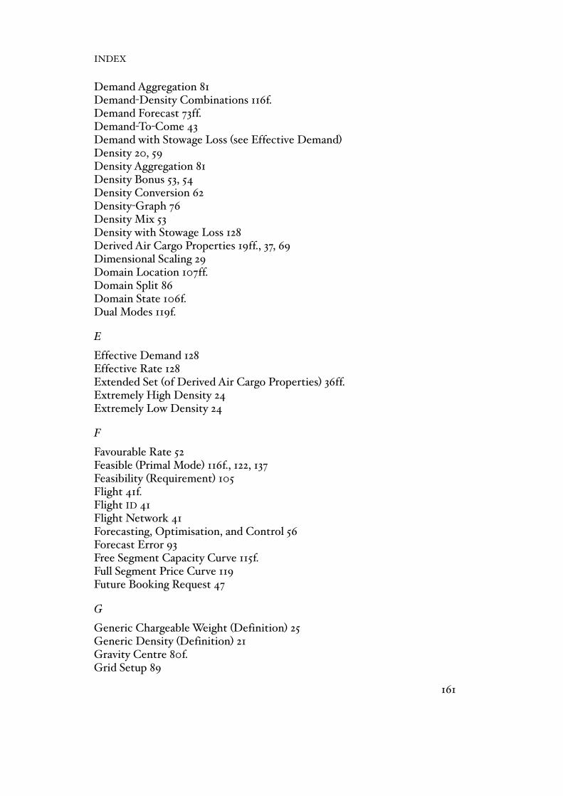
Demand Aggregation 81Demand-Density Combinations 116f.Demand Forecast 73ff.Demand-To-Come 43Demand with Stowage Loss (see Effective Demand)Density 20, 59Density Aggregation 81Density Bonus 53, 54Density Conversion 62Density-Graph 76Density Mix 53Density with Stowage Loss 128Derived Air Cargo Properties 19ff., 37, 69Dimensional Scaling 29Domain Location 107ff.Domain Split 86Domain State 106f.Dual Modes 119f.

E

Effective Demand 128Effective Rate 128Extended Set (of Derived Air Cargo Properties) 36ff.Extremely High Density 24Extremely Low Density 24

F

Favourable Rate 52Feasible (Primal Mode) 116f., 122, 137Feasibility (Requirement) 105Flight 41f.Flight ID 41Flight Network 41Forecasting, Optimisation, and Control 56Forecast Error 93Free Segment Capacity Curve 115f.Full Segment Price Curve 119Future Booking Request 47

G

Generic Chargeable Weight (Definition) 25Generic Density (Definition) 21Gravity Centre 80f.Grid Setup 89

INDEX

161

H

High Density 23

I

Initial Aggregation Scheme 84f.Initial Air Cargo Properties 19Insufficient Bookable Capacities (see Insufficient Capacities)Insufficient Capacity 96, 101, 106

J, K

Kuhn-Tucker Conditions 104ff.

L

Leg 42Loading Device 125Low Density 23Lumpy Bid Price 114f.Lumpy Demand 49

M

Marginal Bid Price 111ff.Marginal Demand 95f., 101, 106ff.Marginal Segment Price Curve 102ff.Marginal Rate-Density Domains (see Marginal Demand)Medium High Density 24Medium Low Density 24Moderately High Density 24Moderately Low Density 24Modified Aggregation Scheme 86f.

N

Non-Overlapping Domain 84ff., 89Non-Negativity (Requirement) 105Not Feasible (Primal Mode) 116f., 122, 137Not Profitable (Dual Mode) 119f., 122, 137

O

Origin & Destination 41Overlapping Domain 84ff., 89

APPENDIX

162

P

Past Booking Request 47Primal-Dual Graph 120Primal-Dual Graph with Stowage Loss 136Primal-Dual Mode 122f.Primal Modes 116f. Primary Quantity Units (see Quantity Units)Profitability (Requirement) 105Profitable (Dual Mode) 119f., 122, 137Profitable Demand 95f., 101, 106ff.Profitable Rate-Density Domains (see Profitable Demand)Pure Volume 20, 28, 44Pure Weight 20, 28, 44

Q

Quantity Units 15

R

Rate 31, 34f.Rate Aggregation 81Rate-Density Combinations 119fRate-Density Domain 78ff.Rate-Density Grid 89Rate-Graph 76Rate Mix 52f.Rate per Actual Weight 34f.Rate per Chargeable Weight 36Rate with Stowage Loss (see Effective Rate) Regular Density (see Density)RES (see Reservation System) Reservation System 47Revenue 19Reversed Formulas 36Reversed Lumpy Bid Price Decision Rule 119Route-Mix 55

S

Saleable Capacity (see Bookable Capacity)Sales Steering 120Scaled Density 63Secondary Quantity Units (see Quantity Units)Segment 42Segment Demand 43f.

INDEX

163

Segment Level Complementary Slackness Conditions 105f.Segment Reduction (as in ‘Segment-Reduced’) 118Set-Up (of a Rate-Density Grid) 89Short Capacity 53Short Route 55Simple Grid 89Simple Set (of Derived Air Cargo Properties) 34Special Handling Code 126Specific Weight and Volume Consumption 30f.SPL (see Special Handling Code)Standard Density 21f.Stochastic Demand 93Stowage Loss 125, 129Stowage Loss Bar 135Sufficient Bookable Capacities (see Sufficient Capacities)Sufficient Capacity 96, 101, 106Suitable Density 53

T

Three Dimensions of a Booking (Request) 48

U

Unified Density 62Unified Density with Stowage Loss 128Unit Cost 37, 38Universal Economic Term 27f.Unprofitable Demand 95f., 101, 106ff.Unprofitable Rate-Density Domains (see Unprofitable Demand)

V

Volume 19Volume Coefficient 30f.Volume Stowage Loss 125Volume with Stowage Loss 127

W

Weight 19Weight and Balance (Process) 126Weight and Volume Consumption-Graph 77Weight Coefficient 30f.Weight Stowage Loss 125Weighting Factor (of a Booking Request)

APPENDIX

164

X, Y, Z

INDEX

165

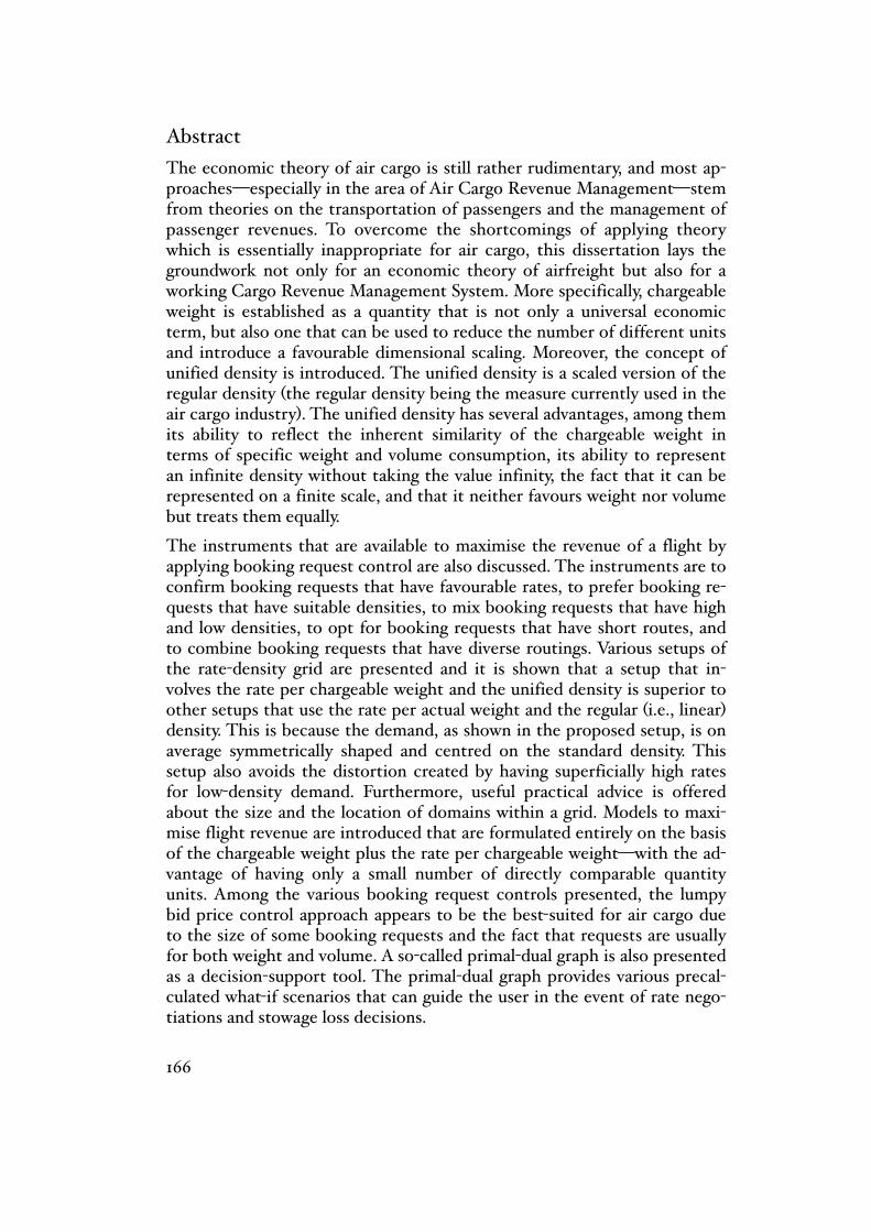
Abstract

The economic theory of air cargo is still rather rudimentary, and most ap-proaches—especially in the area of Air Cargo Revenue Management—stem from theories on the transportation of passengers and the management of passenger revenues. To overcome the shortcomings of applying theory which is essentially inappropriate for air cargo, this dissertation lays the groundwork not only for an economic theory of airfreight but also for a working Cargo Revenue Management System. More specifically, chargeable weight is established as a quantity that is not only a universal economic term, but also one that can be used to reduce the number of different units and introduce a favourable dimensional scaling. Moreover, the concept of unified density is introduced. The unified density is a scaled version of the regular density (the regular density being the measure currently used in the air cargo industry). The unified density has several advantages, among them its ability to reflect the inherent similarity of the chargeable weight in terms of specific weight and volume consumption, its ability to represent an infinite density without taking the value infinity, the fact that it can be represented on a finite scale, and that it neither favours weight nor volume but treats them equally.

The instruments that are available to maximise the revenue of a flight by applying booking request control are also discussed. The instruments are to confirm booking requests that have favourable rates, to prefer booking re-quests that have suitable densities, to mix booking requests that have high and low densities, to opt for booking requests that have short routes, and to combine booking requests that have diverse routings. Various setups of the rate-density grid are presented and it is shown that a setup that in-volves the rate per chargeable weight and the unified density is superior to other setups that use the rate per actual weight and the regular (i.e., linear) density. This is because the demand, as shown in the proposed setup, is on average symmetrically shaped and centred on the standard density. This setup also avoids the distortion created by having superficially high rates for low-density demand. Furthermore, useful practical advice is offered about the size and the location of domains within a grid. Models to maxi-mise flight revenue are introduced that are formulated entirely on the basis of the chargeable weight plus the rate per chargeable weight—with the ad-vantage of having only a small number of directly comparable quantity units. Among the various booking request controls presented, the lumpy bid price control approach appears to be the best-suited for air cargo due to the size of some booking requests and the fact that requests are usually for both weight and volume. A so-called primal-dual graph is also presented as a decision-support tool. The primal-dual graph provides various precal-culated what-if scenarios that can guide the user in the event of rate nego-tiations and stowage loss decisions.

166

Samenvatting

Economische theorie over het vervoer van luchtvracht is nog in het begin-stadium en de meeste aanpakken—vooral op het gebied van revenue ma-nagement van luchtvracht—zijn ontstaan vanuit de theorie van het trans-porteren van passagiers en het revenue management van passagiers. Om de tekortkomingen van deze aanpakken op te vangen, legt dit proefschrift niet alleen de basis voor een economische theorie voor luchtvracht maar ook voor een werkend systeem ten behoeve van het revenue management van luchtvracht. Meer specifiek, chargeable weight (‘te factureren gewicht’) wordt gedefinieerd als een eenheid die niet alleen een universeel econo-misch begrip is, maar ook gebruikt kan worden om een aantal andere een-heden te vermijden en om tot een goed bruikbare schaling te komen. Bo-vendien wordt het concept van de geschaalde dichtheid geïntroduceerd. De geschaalde dichtheid is, zoals de naam al zegt, een geschaalde versie van de normale dichtheid (deze laatste wordt momenteel in de luchtvrachtindus-trie gebruikt). Het gebruik van de geschaalde dichtheid heeft verschillende voordelen, waaronder de mogelijkheid om makkelijk om te gaan met de ge-lijkheid tussen volume en gewicht die bestaat bij het gebruik van chargea-ble weight, de mogelijkheid om een oneindige dichtheid weer te geven, de representatie op een eindige schaal, en de eigenschap dat volume en ge-wicht gelijk behandeld worden.

De hulpmiddelen om de opbrengst van een vrachtvlucht te maximaliseren, door een goede beslissingsstrategie bij de boekingsaanvragen, worden even-eens besproken. Deze hulpmiddelen: bevestigen boekingsaanvragen met gunstige tarieven, hebben de voorkeur voor boekingsaanvragen met ge-schikte dichtheden, mengen boekingsaanvragen met hoge en lage dichthe-den, hebben de voorkeur voor boekingsaanvragen met korte routes, en combineren boekingsaanvragen die verschillende routes hebben. Er worden verschillende vormen van de tarief-versus-dichtheid roosters gepresenteerd, en er wordt aangetoond dat het rooster waarbij het tarief per chargeable kilogram en de geschaalde dichtheid gebruikt worden, superieur is vergele-ken met andere roostervormen (bijvoorbeeld roosters die tarieven per ge-wone kilogram en de normale dichtheid gebruiken). De reden hiervoor is dat de vraag gemiddeld genomen symmetrisch is qua vorm en gecentreerd ligt op de standaard dichtheid. Dit rooster voorkomt ook problemen die ontstaan ten gevolgen van kunstmatig hoge tarieven voor vracht met een lage dichtheid. Verder worden er in dit proefschrift praktische adviezen gegeven met betrekking tot de grootte en de locatie van de tarief- en dichtheidsdomeinen in een rooster.

Modellen die de opbrengst van een vlucht maximaliseren worden bespro-ken. Deze modellen zijn geheel geformuleerd in termen van chargeable weight en de tarieven per chargeable weight, en heeft als voordeel dat slechts enkele grootheden met elkaar vergeleken behoeven te worden.

167

Verschillende strategieën worden besproken voor het afhandelen van boe-kingsaanvragen. De zogenaamde lumpy bid price control lijkt daarbij het meest geschikt voor luchtvracht met name vanwege de grootte van sommi-ge boekingsaanvragen en het feit dat de meeste aanvragen zowel gewicht als volume betreffen. Een primale-duale grafiek is ontwikkeld als een beslis-singsondersteunend hulpmiddel. Deze grafiek bevat verscheidene ‘what-if ’ scenario’s die de gebruiker van een revenue management systeem kunnen begeleiden bij tariefonderhandelingen en stuw-verlies beslissingen.

168

About the Author

Contact Details:

Johannes BlomeyerAm Weißen Berg 561389 Schmitten im [email protected]

Curriculum Vitae:

Date of Birth0 3.5.1961Place of Birth0 Frankfurt am Main1971-19810 0 Goethe Gymnasium Frankfurt (Secondary School)1982-19850 0 Hochschule der Künste Berlin;0 0 0 Studies in Social and Business Communication,0 0 0 graduated with the Master’s Degree0 0 0 ‘Diplom-Kommunikationswirt’1985-19930 0 Johann Wolfgang Goethe-Universität Frankfurt;0 0 0 Studies in Economics, 0 0 0 graduated with the Master’s Degree0 0 0 ‘Diplomkaufmann’1993-19980 0 Lecturer at Logo Repetitorium der Wirtschafts-0 0 0 wissenschaften, Frankfurt1998-20050 0 Revenue Research Analyst, Lufthansa Cargo AG

2005-present0 Crew Scheduling Analyst, Lufthansa Passage AG

169

Air Cargo Revenue Management

Documents

Transcript of Air Cargo Revenue Management