The Transmission Mechanism of Governemnt Spending in Ghana: Empirical Analysis and Policy...

The Transmission Mechanism of Government Spending inGhana: Empirical Analysis and Policy Implications

Said Boakye1, Ph.D.Technical Advisor (Macroeconomist)

Ministry of Finance and Economic Planning of the Republic of Ghana

April, 2009

Abstract

Using a vector autoregression (VAR) model and a vector error correctionmodel (VECM), this paper presents an empirical analysis of the transmis-sion mechanism of government spending in Ghana. It also discusses policyimplications of the empirical �ndings. Cointegration estimation and in-novation analysis in the form of impulse response functions and variancedecompositions are used to study the e¤ects, the channels of the e¤ects andthe timing of the e¤ects of government spending in Ghana. Some of the�ndings of the study are as follows: 1) A total government spending shockhas only a one-period positive e¤ect on real output because of the crowding-out e¤ect of the cedi exchange rate. 2) Real GDP growth is a very reliablemeans of achieving macroeconomic stability in Ghana. 3) Money and thusin�ation are largely neutral in Ghana as they have no impact on real GDP.4) Increase in real interest rate has no signi�cant e¤ect on money supply inGhana. It however causes the price level to increase because it contractsreal GDP. Two of the policy implications of the �ndings are that: 1) ef-forts should be made to restrict government spending increases in Ghana,especially those �nanced through borrowing 2) increase in interest rate asa means of �ghting in�ation should be avoided.

1 I am very grateful to Mr. Samuel Arkhurst of the Ministry of Finance and EconomicPlanning and Mr. Duncan of Ghana Statistical Service for giving to me some of the dataI used.

1

1. Introduction

Government spending can have very powerful positive and negativee¤ects on the economy. Ensuring e¤ective �scal policy formulation andimplementation therefore requires in-depth empirical knowledge of thetransmission mechanism of government spending. Thus, to achievee¤ective macroeconomic management in terms of macroeconomic sta-bility and real output growth through �scal policy, policy makers needto have strong empirical knowledge of the e¤ects, the channels of thee¤ects and the timing of the e¤ects of government spending on macro-economic variables. In spite of this, the existing research work andpolicy papers about the economy of Ghana have not considered thisvery important topic as their main focus. The existing empirical stud-ies about the Ghanaian economy mostly deal with other importanttopics such as macroeconomic forecasting (see, for instance, Abbeyand Clark (1974), Ghartey and Rao (1990), Atta-Mensah and Bawu-mia (2003)); monetary policy issues (see, for instance, Ghartey (1998),Abradu-Otoo, Amoah and Bawumia (2003)); and international tradeand balance of payment (see, for instance, Amoako (1980), Ghartey(1987), Leith (1974)).

This paper is therefore intended to help �ll this gap, and to serveas a source of reference for �scal policy discussions. One study aboutthe Ghanaian economy that is closely related to this work is Ghartey(2001). Among other things, Ghartey (2001) investigates the in�a-tionary nature of de�cit �nancing in Ghana.

The need for empirical research into the transmission mechanismof government spending for the purpose �scal policy formulation andimplementation is made pressing by the con�icting nature of the variouseconomic theories that explain the impact of government spending onthe economy. This implies that to achieve a more e¤ective �scal policyformulation and implementation, policy makers cannot entirely rely oneconomic theory.

The "expansionary �scal contraction" hypothesis proposed by Barryand Devereux (1995), Sutherland (1997), Perotti (1999), etc. arguesthat increases in government spending can have a very weak or even acontractionary e¤ect on real output in the face of large �scal de�citsand huge public debt. This is because large �scal de�cits and hugepublic debt generate expectations of a looming �scal crisis. As aresult, further increase in government spending may lead to decreasesin private consumption and investment and thus real output.

2

Standard Keynesian theory on the other hand argues that govern-ment spending shocks can be a very powerful means to achieve ac-celerated real output growth because it stimulates aggregate demandand generates rounds and rounds of income through the multiplier ef-fect. However, this theory is based on strong assumptions of pricerigidity and the existence of excess capacity. Yet, recent empiricalstudies have found that in developing countries like Ghana, prices tendto be very �exible because of institutional and structural constraintson production, and thus even short-run aggregate supply tends to bevery inelastic. This means that government spending shocks are morelikely to generate in�ationary pressures than to bring about real outputgrowth in developing economies.

In addition to price �exibility, it is well understood that govern-ment spending shocks crowd out private investment and consumptionand thus real output through increase in interest rate in the loanablefunds and money markets. In the loanable funds market, increase ingovernment spending, holding other factors constant, brings about de-crease in national savings and thus supply of loanable funds therebycreating shortage of funds, which pushes up interest rate. In the moneymarket, the increase in income generated through the multiplier e¤ectbrings about increase in demand for money, which, holding constantsupply of money, brings about increase in interest rate. Another sourceof crowding-out e¤ect of increase in government spending on real out-put is depreciation of the domestic currency in the foreign exchangemarket. Depreciation of the domestic currency makes imported rawmaterials and other imported capital inputs become expensive, whichbrings about increase in costs of production of �rms and therefore de-crease in real output. Increase in government spending may lead todepreciation of the domestic currency through at least two channels:First, the increase in government spending itself may directly includeincrease in foreign purchases of goods and services as well as increase ingovernment foreign debt servicing. These components of governmentspending increase bring about increase in demand for foreign currency,which leads to depreciation of the domestic currency. Second, theinitial increase in income generated through the multiplier e¤ect maylead to increase in imports and therefore increase in demand for foreigncurrencies leading to depreciation of the domestic currency.

Therefore, the e¤ectiveness of government spending shocks to stim-ulate real GDP growth depends on factors such us price elasticity ofaggregate supply, interest elasticity of money demand, interest elas-ticity of investment, imports elasticity of income, the size of increasein government foreign purchases and debt servicing, the size of public

3

debt, etc. Because these factors di¤er from one country to another asthey are in�uenced by country-speci�c factors such as structural andinstitutional development and arrangements, we need country-speci�cempirical studies to inform �scal policy formulation and implementa-tion.

I utilize cointegration estimation and innovation analysis in the formof impulse-response functions and variance decompositions to analyzethe e¤ects, the channels of the e¤ects, and the timing of the e¤ects ofgovernment spending shock (and shocks to other variables) on macro-economic variables in Ghana. I carry out the analysis via a vector au-toregression (VAR) model and a derived vector error correction model(VECM). Since I �nd all the variables to be integrated of order 1,I justify the use of the VAR and the VECM by testing and �ndingcointegrating relations among the variables.

The rest of the paper is organized as follows. Section 2 discussesthe selection of the variables and the data used for the study. Section3 describes the model. Section 4 performs unit root and cointegratingrank tests. Section 4 also presents and discusses the results for thecointegration estimation. Section 5 discusses the innovation analysis.Section 6 continues the innovation analysis by disaggregating real gov-ernment spending into real government consumption spending and realgovernment capital spending. Section 7 discusses policy implicationsof the �ndings, and section 8 concludes the paper.

2. Variables Selection and Data

2.1. Variables Selection

The core variables used for the study are per-capita real govern-ment expenditure (PCRGE), per-capita real GDP (PCRGDP ), theprice level as measured by GDP de�ator (GDPDEFL), the cedi ex-change rate as measured by the bilateral exchange rate between thecedi and the US dollar (EXR), and real interest rate (RINTR). LikeAtta-Mensa and Bawumiah (2003), interest rate in this study is repre-sented by the treasury bill rate. I consider these variables to be corebecause they consistently feature in theoretical discussions about thee¤ects of �scal policy variables on the economy. Additionally, variouscombinations of these variables are frequently used in the empirical lit-erature on the transmission mechanism of �scal policy variables (see,for instance, Perotti (2005), Kandil (2006), etc). The real variableswere generated by de�ating their respective nominal values by the GDPde�ator. In the case of real interest rate, the rate of change of the GDP

4

de�ator was used to de�ate the nominal interest rate. The exchangerate is in terms of the number of cedis needed to exchange for one USdollar. Because of this, increase in the exchange rate implies depreci-ation of the cedi, and vice versa. Ghartey (2001) argues that, prior to1998, interest rate was �xed by the government, and up to 1996, theBank of Ghana�s open market operation rendered it almost worthless.However, I included real interest rate because of its theoretical signif-icance as a channel by which government spending shocks a¤ect theeconomy.

To be able to isolate the true e¤ects of government spending onmacroeconomic variables in Ghana, I control for monetary policy byincluding per-capita money supply (PCM2). Because of this, I alsodiscuss monetary policy issues in this paper.

2.2. The Data

The Ghana Statistical Service, the Ministry of Finance and Eco-nomic Planning of Ghana, the International Financial Statistics onlineof the IMF, and the World Development Indicators online of the WorldBank are the sources of the data for this study. The sample coversquarterly values from 1983 to 2007: 1983q1 to 2007q4. The dataon interest rate, exchange rate and money supply were in quarterlyseries from the source. However, the data on per-capita GDP, per-capita government expenditure, and GDP de�ator were originally inannual series, and I converted them into quarterly series. With theexception of real interest rate (RINTR), I converted all the variablesinto logarithms. The endogenous variables are therefore LPCRGDP ,LGDPDEFL, LEXR, RINTR, LPCRGE and LPCM2. Thus, the "L"at the beginning of the names of the variables stands for logarithm.

Figures 1a, 1b, 1c, 1d, 1e and 1f below show the line graphs of thevariables. It can be seen from these graphs that most of the variablesshow apparent deterministic time trend in them.

5

Fig. 1a: LPCRGE Fig. 1b: LPCRGDP Fig. 1c: LGDPDEFL

3.2

3.6

4.0

4.4

4.8

5.2

5.6

84 86 88 90 92 94 96 98 00 02 04 06

LPCRGE

5.9

6.0

6.1

6.2

6.3

6.4

6.5

84 86 88 90 92 94 96 98 00 02 04 06

LPCRGDP

3

4

5

6

7

8

9

10

84 86 88 90 92 94 96 98 00 02 04 06

LGDPDEFL

Fig. 1d: LEXR Fig. 1e: RINTR Fig. 1f: LPCM2

3

4

5

6

7

8

9

10

84 86 88 90 92 94 96 98 00 02 04 06

LEXR

4

8

12

16

20

24

28

32

36

40

84 86 88 90 92 94 96 98 00 02 04 06

RINTR

7

8

9

10

11

12

13

14

15

84 86 88 90 92 94 96 98 00 02 04 06

LPCM2

3. The empirical Model

Let the following VAR(p) be the representation of the dynamic re-lation among the variables:

Xt = A1Xt�1+A2Xt�2+:::::+ApXt�p+DZt+�t (1) where

Xt = [LPCRGDPt LGDPDEFLt LEXRt RINTRt LPCRGEt LPCM2t]0,

Ai is a 6� 6matrix of coe¢ cients for the lagged vector Xt�i, Zt is a vec-tor of deterministic components (constant drift term and deterministictime trend), D is a matrix of coe¢ cients for the deterministic compo-nents, and �t is a 6 � 1 vector of innovations. Suppose that all thevariables in Xt are I(1)2. Model (1) can be rewritten as a vector errorcorrection model (VECM) as follows:

�Xt = �Xt�1 +

p�1Xi=1

�i�Xt�1 + DZt + �t (2)

where � =

pXi=1

Ai � I; and �i = �pX

j=i+1

Aj. If the rank r of � is

2This assumption is veri�ed in the next section.

6

zero (rank(�)= 0), then there is no long-run equilibrium (cointegrat-ing) relation among the variables. In this case, regression based onthe above models is spurious with correlated error terms. If rank(�)= 6, then it is the case of full rank and the variables would be station-ary or integrated of order 0 and not I(1) as assumed. Now, if 0 <rank(�) < 6, then there is/are cointegrating or long-run equilibriumrelation(s) among the variables. In this case, by Granger�s represen-tation theorem, there exists 6� r matrices � and � each having rankr such that � = ��, and �0Xt is I(0). The elements of � in model (2)

are adjustment parameters measuring deviations of the variables fromtheir long-run trends, and each column of � is the cointegrating vec-tor or vector of long-run parameters. r is the number of cointegrating(long-run equilibrium) relations or the cointegrating rank.

4 Unit Root and Cointegrating Rank Tests, and CointegrationEstimation

It is clear from the discussion in section 3 that to achieve reliableinferences based on estimates of parameters from the above models,we should ensure that if the variables are proved to be integrated oforder 1, then there exists cointegrating relations among the variables.I therefore determine the order of integration of the series and checkfor existence of cointegrating relations in this section.

4.1 Unit Root Tests

I determine the order of integration of the series by employing theaugmented Dickey-Fuller (ADF) unit root testing procedure. Withthe exception of LPCRGE, I include a drift term and a deterministictime trend in the ADF equation because of the apparent time trend inthe series as shown by the line graphs in subsection 2.2. Thus, I testfor the presence of unit roots in the levels of the variables using thefollowing ADF equation3:

�xt = c+ bTIME + (�� 1)xt�1 +PLj=1 j�xt�j + "t (3)

3For LPCRGE the ADF equation is �xt = c+axt�1+PL

j=1 j�xt�j + "t In-cluding a time trend in the ADF equation for LPCRGE leads to the rejection of the nullhypothesis of existence of unit root (nonstationarity) in the series. This suggests thatLPCRGE has a stochastic trend and not a deterministic trend.

7

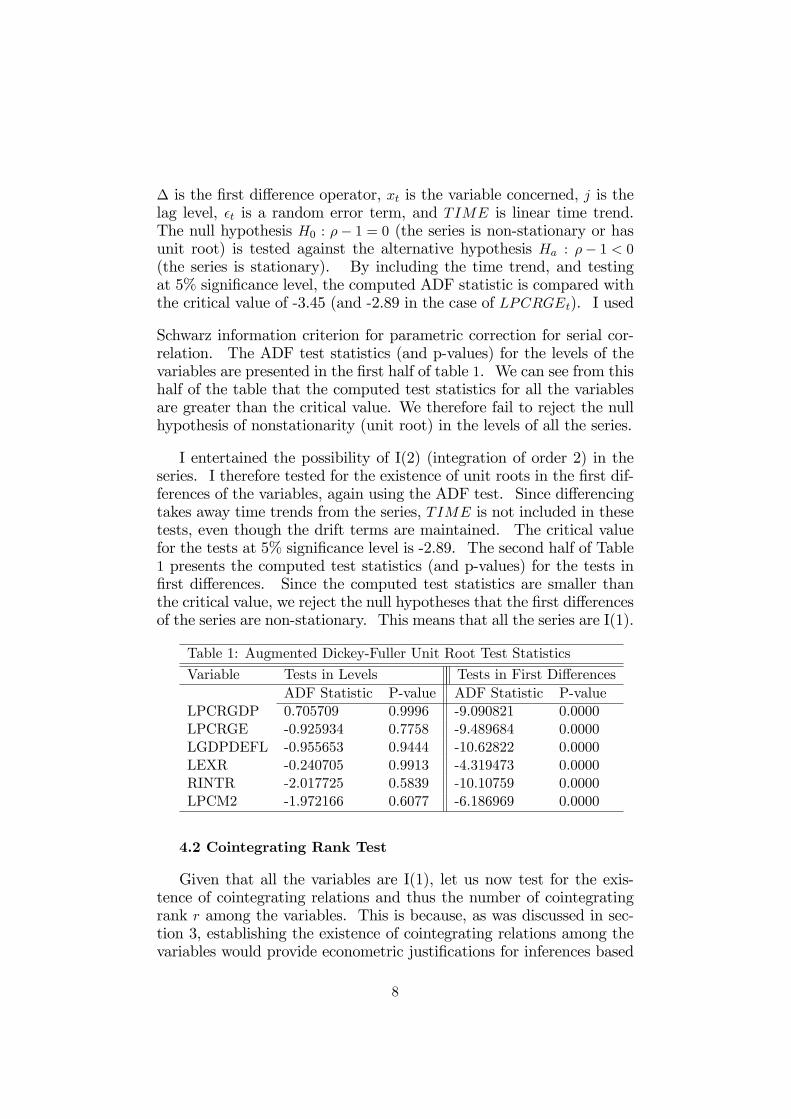
where� is the �rst di¤erence operator, xt is the variable concerned, j is thelag level, �t is a random error term, and TIME is linear time trend.The null hypothesis H0 : �� 1 = 0 (the series is non-stationary or hasunit root) is tested against the alternative hypothesis Ha : �� 1 < 0(the series is stationary). By including the time trend, and testingat 5% signi�cance level, the computed ADF statistic is compared withthe critical value of -3.45 (and -2.89 in the case of LPCRGEt). I used

Schwarz information criterion for parametric correction for serial cor-relation. The ADF test statistics (and p-values) for the levels of thevariables are presented in the �rst half of table 1. We can see from thishalf of the table that the computed test statistics for all the variablesare greater than the critical value. We therefore fail to reject the nullhypothesis of nonstationarity (unit root) in the levels of all the series.

I entertained the possibility of I(2) (integration of order 2) in theseries. I therefore tested for the existence of unit roots in the �rst dif-ferences of the variables, again using the ADF test. Since di¤erencingtakes away time trends from the series, TIME is not included in thesetests, even though the drift terms are maintained. The critical valuefor the tests at 5% signi�cance level is -2.89. The second half of Table1 presents the computed test statistics (and p-values) for the tests in�rst di¤erences. Since the computed test statistics are smaller thanthe critical value, we reject the null hypotheses that the �rst di¤erencesof the series are non-stationary. This means that all the series are I(1).

Table 1: Augmented Dickey-Fuller Unit Root Test Statistics

Variable Tests in Levels Tests in First Di¤erencesADF Statistic P-value ADF Statistic P-value

LPCRGDP 0.705709 0.9996 -9.090821 0.0000LPCRGE -0.925934 0.7758 -9.489684 0.0000LGDPDEFL -0.955653 0.9444 -10.62822 0.0000LEXR -0.240705 0.9913 -4.319473 0.0000RINTR -2.017725 0.5839 -10.10759 0.0000LPCM2 -1.972166 0.6077 -6.186969 0.0000

4.2 Cointegrating Rank Test

Given that all the variables are I(1), let us now test for the exis-tence of cointegrating relations and thus the number of cointegratingrank r among the variables. This is because, as was discussed in sec-tion 3, establishing the existence of cointegrating relations among thevariables would provide econometric justi�cations for inferences based

8

on estimates from models (1) and (2). I use Johansen�s cointegratingrank testing approach.

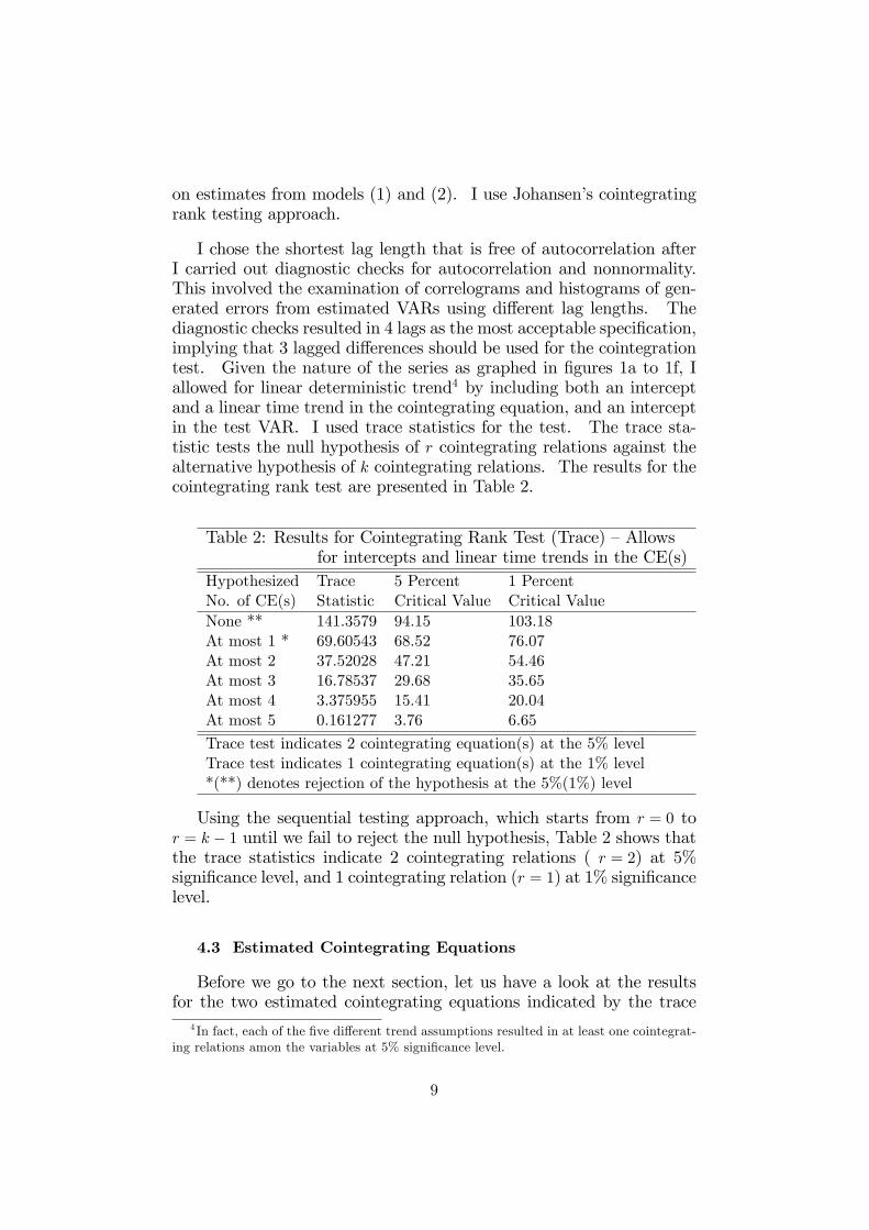
I chose the shortest lag length that is free of autocorrelation afterI carried out diagnostic checks for autocorrelation and nonnormality.This involved the examination of correlograms and histograms of gen-erated errors from estimated VARs using di¤erent lag lengths. Thediagnostic checks resulted in 4 lags as the most acceptable speci�cation,implying that 3 lagged di¤erences should be used for the cointegrationtest. Given the nature of the series as graphed in �gures 1a to 1f, Iallowed for linear deterministic trend4 by including both an interceptand a linear time trend in the cointegrating equation, and an interceptin the test VAR. I used trace statistics for the test. The trace sta-tistic tests the null hypothesis of r cointegrating relations against thealternative hypothesis of k cointegrating relations. The results for thecointegrating rank test are presented in Table 2.

Table 2: Results for Cointegrating Rank Test (Trace) �Allowsfor intercepts and linear time trends in the CE(s)

Hypothesized Trace 5 Percent 1 PercentNo. of CE(s) Statistic Critical Value Critical ValueNone ** 141.3579 94.15 103.18At most 1 * 69.60543 68.52 76.07At most 2 37.52028 47.21 54.46At most 3 16.78537 29.68 35.65At most 4 3.375955 15.41 20.04At most 5 0.161277 3.76 6.65

Trace test indicates 2 cointegrating equation(s) at the 5% levelTrace test indicates 1 cointegrating equation(s) at the 1% level*(**) denotes rejection of the hypothesis at the 5%(1%) level

Using the sequential testing approach, which starts from r = 0 tor = k � 1 until we fail to reject the null hypothesis, Table 2 shows thatthe trace statistics indicate 2 cointegrating relations ( r = 2) at 5%signi�cance level, and 1 cointegrating relation (r = 1) at 1% signi�cancelevel.

4.3 Estimated Cointegrating Equations

Before we go to the next section, let us have a look at the resultsfor the two estimated cointegrating equations indicated by the trace

4 In fact, each of the �ve di¤erent trend assumptions resulted in at least one cointegrat-ing relations amon the variables at 5% signi�cance level.

9

test at 5% signi�cance level. These equations were estimated via theVECM. The variables were listed in the following order5: LPCRGDP tLEXRt LGDPDEFLt RINTRt LPCRGEt LPCM2t.

Table 3 presents the cointegration estimation results. We cansee from table 3 that in Ghana, an increase in government spendingsigni�cantly brings about depreciation of the Cedi in the long run.And because the cedi depreciates, real GDP is crowded out6, makingincrease in government spending have a negative e¤ect on real outputin the long run in Ghana. Money supply on the other hand hasinsigni�cant e¤ects on real GDP and the cedi exchange rate in the longrun. The insigni�cant e¤ect of money supply on real output in thelong run in Ghana con�rms the classical neutrality of money �money,a nominal variable, has no e¤ect on real variables. Again, we cansee from table 3 that increase in the price level (in�ation) signi�cantlyincreases the exchange rate in the long run. However, in�ation hasinsigni�cant e¤ect on real output in the long run in Ghana. Finally,table 3 shows that increase in real interest rate signi�cantly decreasesreal output and the cedi exchange rate in Ghana in the long run.

Table 3: Results for the Cointegrating Eqs EstimationReal GDP The Cedi Exch. Rate

Constant 6:75 �20:74Time Trend 0:011��

(2:06)�0:187��(�7:10)

Price Level �0:067(�0:61)

2:97��(5:23)

Real Interest Rate �0:003��(�4:19)

�0:026��(�6:21)

Gov�t Expenditure �0:264��(�3:75)

3:73��(10:25)

Money Supply 0:055(0:86)

0:076(0:23)

The values in parentheses are t-statistics.*** and ** stand for signi�cance at 1% and 5%

signi�cance levels respectively.

5 Innovation Analysis and the Transmission Mechanism

Let us now utilize impulse response functions and variance decom-positions to analyze how a government spending shock a¤ects the econ-omy of Ghana. To fully understand the e¤ects, the channels of the

5Even though I get the same number of cointegrating rank from the trace test whenLGDPDEFL is listed before LEXR, the estimated cointegrating equations make moreeconomic sence when LEXR is listed before LGDPDFL.

6 I will provide a demonstration for this statement in the next section.

10

e¤ects and the timing of the e¤ects of a shock to government spend-ing on the Ghanaian economy, we shall also consider shocks to theother variables. I use Cholesky decomposition method with the fol-lowing ordering: LPCRGEt LPCM2t LGDPDEFLt RINTRt LEXRtLPCRGDP t. Thus, like Fatás and Mihov (2001), I use Choleski order-ing as a means of identifying government spending shocks by orderingit �rst. However, di¤erent oderings do not signi�cantly change theresults.

5.1 Impulse Response Functions

To get computed standard errors for the impulse response coe¢ -cients in order to be able to distinguish signi�cant e¤ects from in-signi�cant ones, I carry out the innovation analysis via the vector au-toregression model (VAR) instead of the vector error correction model(VECM). After all, VAR in log-levels is an appropriate representationfor the dynamic relations among a set of cointegrated variables. Thetwo symmetric standard error bands are included in the impulse re-sponse functions. The standard errors were computed using analytic(asymptotic) approach.

5.1.1 E¤ects of a Government Spending Shock

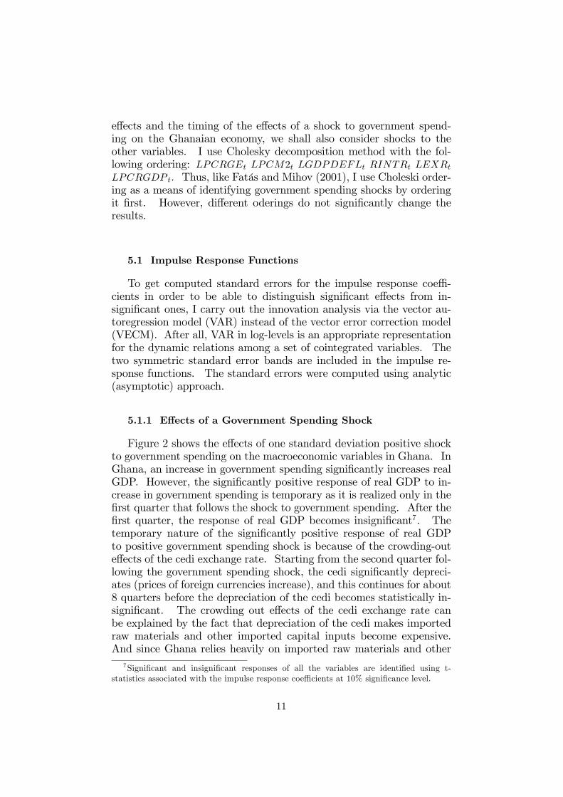
Figure 2 shows the e¤ects of one standard deviation positive shockto government spending on the macroeconomic variables in Ghana. InGhana, an increase in government spending signi�cantly increases realGDP. However, the signi�cantly positive response of real GDP to in-crease in government spending is temporary as it is realized only in the�rst quarter that follows the shock to government spending. After the�rst quarter, the response of real GDP becomes insigni�cant7. Thetemporary nature of the signi�cantly positive response of real GDPto positive government spending shock is because of the crowding-oute¤ects of the cedi exchange rate. Starting from the second quarter fol-lowing the government spending shock, the cedi signi�cantly depreci-ates (prices of foreign currencies increase), and this continues for about8 quarters before the depreciation of the cedi becomes statistically in-signi�cant. The crowding out e¤ects of the cedi exchange rate canbe explained by the fact that depreciation of the cedi makes importedraw materials and other imported capital inputs become expensive.And since Ghana relies heavily on imported raw materials and other

7Signi�cant and insigni�cant responses of all the variables are identi�ed using t-statistics associated with the impulse response coe¢ cients at 10% signi�cance level.

11

imported capital inputs for production, costs of production of �rmsincrease, which leads to decrease in output.

Figure 2: E¤ects of Positive Government Spending Shock

.004

.002

.000

.002

.004

2 4 6 8 10 12 14 16 18 20

Response of LPCRGDP to LPCRGE

.02

.01

.00

.01

.02

.03

2 4 6 8 10 12 14 16 18 20

Response of LGDPDEFL to LPCRGE

.08

.04

.00

.04

.08

2 4 6 8 10 12 14 16 18 20

Response of LEXR to LPCRGE

1.5

1.0

0.5

0.0

0.5

1.0

1.5

2.0

2 4 6 8 10 12 14 16 18 20

Response of RINTR to LPCRGE

.03

.02

.01

.00

.01

.02

.03

.04

2 4 6 8 10 12 14 16 18 20

Response of LPCRGE to LPCRGE

.02

.01

.00

.01

.02

.03

.04

2 4 6 8 10 12 14 16 18 20

Response of LPCM2 to LPCRGE

Response to Cholesky One S.D. Innovations ± 2 S.E.

During the �rst quarter that follows the positive shock to govern-ment spending, the price level responds negatively. This is as a resultof the temporary expansion in real output in response to the posi-tive shock to real government spending. After the �rst quarter, theresponse of the price level becomes insigni�cant for a while. How-ever, it starts to increase from the �fth quarter following the spend-ing shock and this becomes statistically signi�cant after the seventhquarter. The signi�cantly higher price level resulting from the spend-ing shock becomes persistent for about one and a half years beforethe response becomes insigni�cant. A cause of the higher price level(in�ation) is the persistent depreciation of the cedi8 that follows thespending shock.

The response of real interest rate to spending shock is insigni�cantacross time. Money supply responds positively to a positive gov-ernment spending shock. The positive response of money supply isstatistically signi�cant during the sixth quarter and from the ninth tothe eleventh quarter following the spending shock. The increase inmoney supply is a contributing factor (in addition to the depreciation

8 I shall demonstrate the soundness of this statement in the next subsection.

12

of the cedi) to the higher price level that emerges after the spendingshock. Also, the increase in money supply demonstrates the highcentral bank �nancing of excess government spending(over revenue)in Ghana. For instance, in 2000, Bank of Ghana�s �nancing of gov-ernment budget de�cit was as high as 6.6% of GDP (see Amoah andLoloh, 2008). The Bank of Ghana�s Act of 2002 and the West AfricanMonetary Zone�s (WAMZ) criterion that impose restrictions on Bankof Ghana�s �nancing of excess government spending are therefore veryappropriate.

5.1.2 Demonstrating the Crowding-out and the In�ationaryE¤ects of the Cedi Exchange Rate

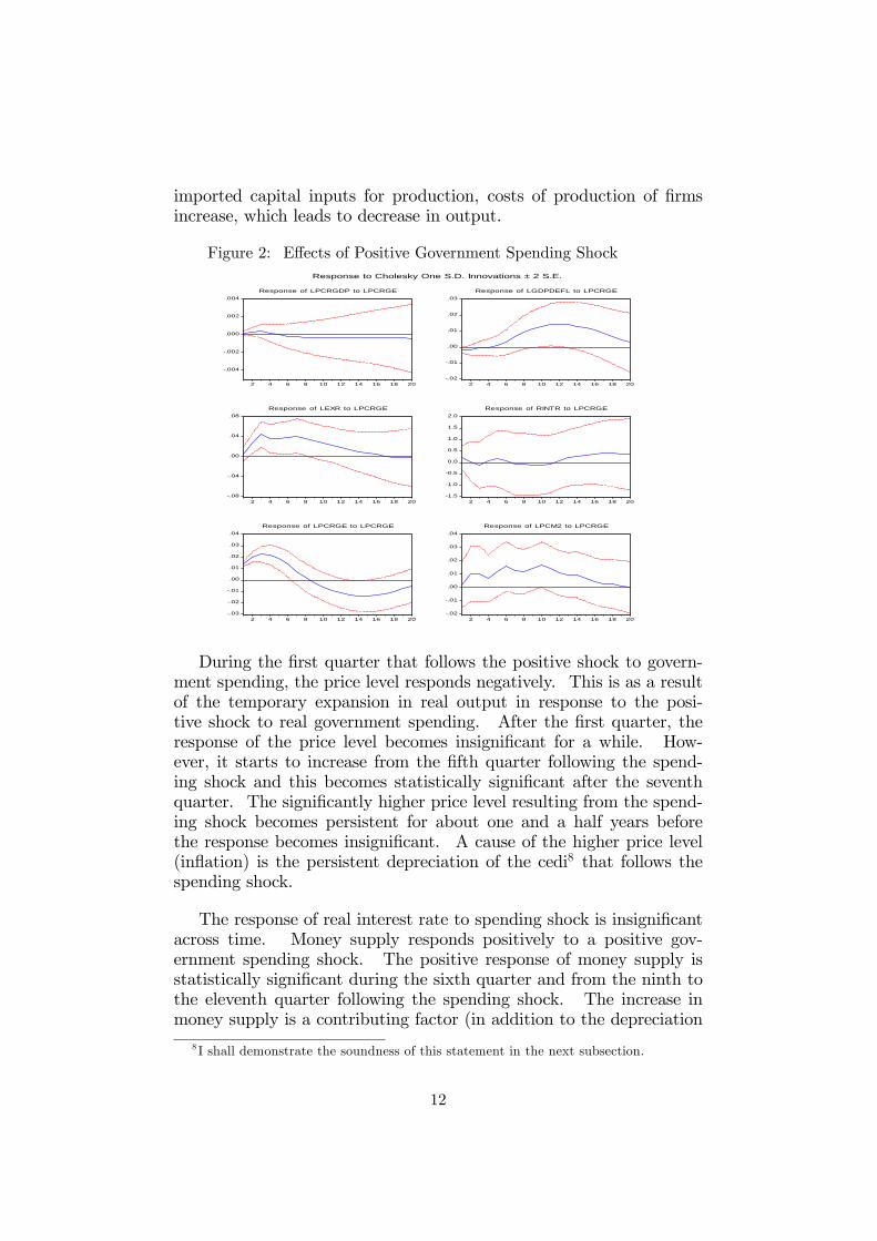
I argued in subsection 5.1.1 that the depreciation of the cedi thatpicks up starting from the second quarter following the spending shockis the cause of the crowding-out e¤ect on real GDP. Additionally, Iargued that depreciation of the cedi is a channel by which a positiveshock to government spending causes in�ation in Ghana. In this sub-section, I demonstrate the soundness of these arguments. I do this byconsidering the e¤ects of a positive shock to the exchange rate of thecedi. Figure 3 shows the e¤ects of a one standard deviation positiveshock to the cedi exchange rate.

Figure 3: The Crowding-out and the In�ationary E¤ectsof the Cedi Exchange Rate

.010

.008

.006

.004

.002

.000

.002

2 4 6 8 10 12 14 16 18 20

Response of LPCRGDP to LEXR

.01

.00

.01

.02

.03

.04

2 4 6 8 10 12 14 16 18 20

Response of LGDPDEFL to LEXR

2

1

0

1

2

3

4

2 4 6 8 10 12 14 16 18 20

Response of RINTR to LEXR

.04

.00

.04

.08

.12

.16

2 4 6 8 10 12 14 16 18 20

Response of LEXR to LEXR

.01

.00

.01

.02

2 4 6 8 10 12 14 16 18 20

Response of LPCRGE to LEXR

.02

.01

.00

.01

.02

.03

.04

.05

2 4 6 8 10 12 14 16 18 20

Response of LPCM2 to LEXR


It can be seen from �gure 3 that real GDP responds negatively to thepositive shock to the cedi exchange rate. In fact, the negative response

13

of real GDP to the positive shock to the exchange rate of the cedi isvery persistent as it is statistically signi�cant starting from the �rstquarter following the exchange rate shock to the eighteenth quarter.This therefore validates the argument that the depreciation of the cedithat shows up starting from the second quarter of government spendingshock crowds out real output.

The price level as measured by GDP de�ator starts to signi�cantlyincrease in statistical terms from the 6th quarter following the positiveshock to the cedi exchange rate, and this continues till the 16th quar-ter. This shows that a channel of the in�ationary e¤ect of governmentspending is the exchange rate of the cedi. Interestingly, the upwardmovement of money supply following the positive exchange rate shockas shown in Figure 3 is not statistically signi�cant at any point in time.This suggests that the in�ationary e¤ect of the exchange rate shock ismostly cost of production or supply induced.

Another interesting e¤ect of a positive shock to the exchange rateof the cedi is that government spending signi�cantly increases (for 4quarters starting from the second quarter). This can be explained bythe fact that, in cedi terms, imports by government and governmentforeign debt servicing become costly making government spending goup when the cedi depreciates.

5.1.3 Should We Be Scared of In�ation in Ghana?

Even though there is always a huge public outcry when there is in-�ation, in�ation, at least in its mild form as we experience in Ghana,is not a menace on its own. The reason is that all nominal economicvariables adjust to re�ect increase in the price level in the long run.Because of this, in�ation has a neutral e¤ect on real economic vari-ables in the long run. This is a form of the so-called neutrality ofmoney. In�ation therefore may be a sign of poor economic perfor-mance (contraction in output) and should thus be scared of, it is notthe source of poor economic performance.

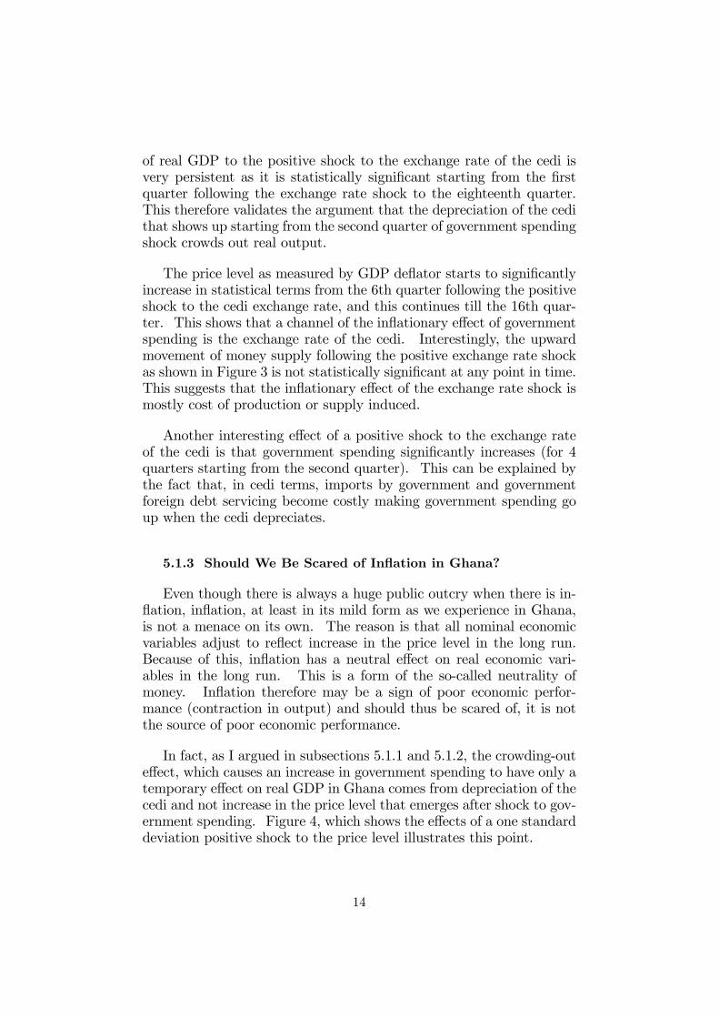
In fact, as I argued in subsections 5.1.1 and 5.1.2, the crowding-oute¤ect, which causes an increase in government spending to have only atemporary e¤ect on real GDP in Ghana comes from depreciation of thecedi and not increase in the price level that emerges after shock to gov-ernment spending. Figure 4, which shows the e¤ects of a one standarddeviation positive shock to the price level illustrates this point.

14

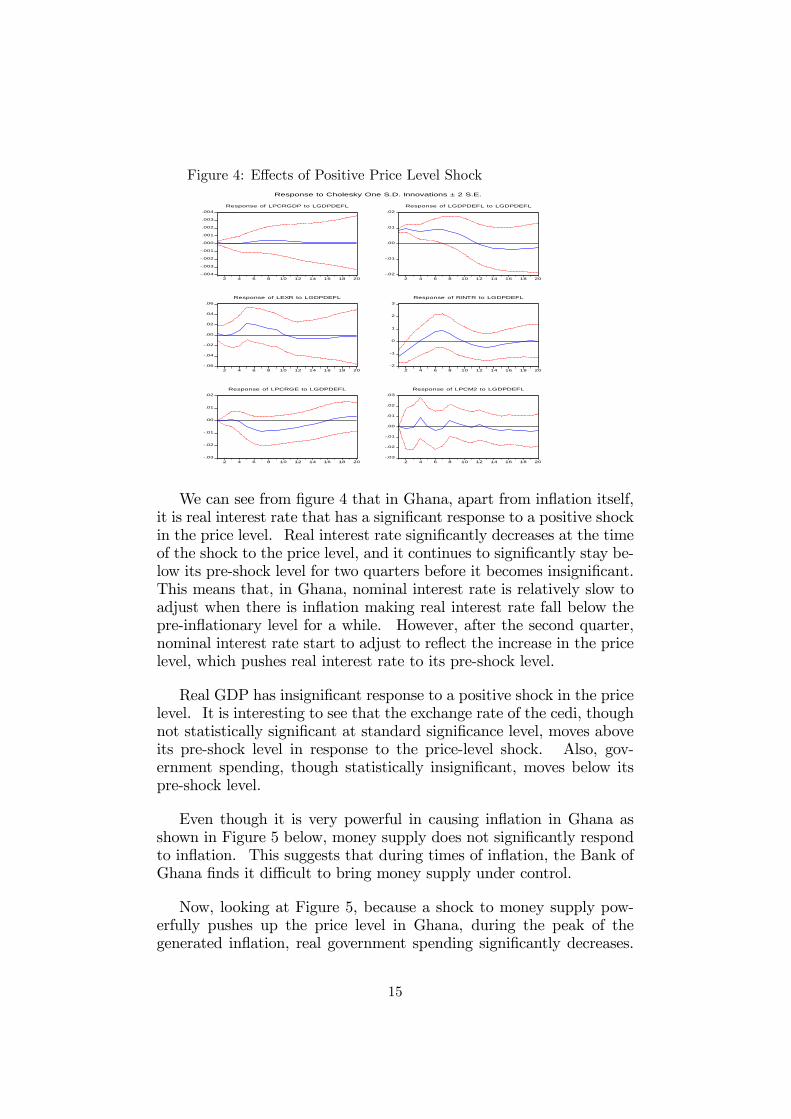
Figure 4: E¤ects of Positive Price Level Shock

.004

.003

.002

.001

.000

.001

.002

.003

.004

2 4 6 8 10 12 14 16 18 20

Response of LPCRGDP to LGDPDEFL

.02

.01

.00

.01

.02

2 4 6 8 10 12 14 16 18 20

Response of LGDPDEFL to LGDPDEFL

.06

.04

.02

.00

.02

.04

.06

2 4 6 8 10 12 14 16 18 20

Response of LEXR to LGDPDEFL

2

1

0

1

2

3

2 4 6 8 10 12 14 16 18 20

Response of RINTR to LGDPDEFL

.03

.02

.01

.00

.01

.02

2 4 6 8 10 12 14 16 18 20

Response of LPCRGE to LGDPDEFL

.03

.02

.01

.00

.01

.02

.03

2 4 6 8 10 12 14 16 18 20

Response of LPCM2 to LGDPDEFL


We can see from �gure 4 that in Ghana, apart from in�ation itself,it is real interest rate that has a signi�cant response to a positive shockin the price level. Real interest rate signi�cantly decreases at the timeof the shock to the price level, and it continues to signi�cantly stay be-low its pre-shock level for two quarters before it becomes insigni�cant.This means that, in Ghana, nominal interest rate is relatively slow toadjust when there is in�ation making real interest rate fall below thepre-in�ationary level for a while. However, after the second quarter,nominal interest rate start to adjust to re�ect the increase in the pricelevel, which pushes real interest rate to its pre-shock level.

Real GDP has insigni�cant response to a positive shock in the pricelevel. It is interesting to see that the exchange rate of the cedi, thoughnot statistically signi�cant at standard signi�cance level, moves aboveits pre-shock level in response to the price-level shock. Also, gov-ernment spending, though statistically insigni�cant, moves below itspre-shock level.

Even though it is very powerful in causing in�ation in Ghana asshown in Figure 5 below, money supply does not signi�cantly respondto in�ation. This suggests that during times of in�ation, the Bank ofGhana �nds it di¢ cult to bring money supply under control.

Now, looking at Figure 5, because a shock to money supply pow-erfully pushes up the price level in Ghana, during the peak of thegenerated in�ation, real government spending signi�cantly decreases.

15

However, the government of Ghana corrects the shortfall in real gov-ernment spending by pushing it up to its pre-shock level. The cediexchange rate signi�cantly increases in response to a shock to moneysupply only in the second quarter following the shock. The cedi depre-ciates in response to the positive shock to money supply because thepowerfully generated in�ation makes imported goods become relativelycheaper. This therefore brings about increase in imports, which putsupward pressures on prices of foreign currencies.

Note from Figure 5 that the in�ation generated by increase in moneysupply is not sudden, unlike the positive shock to the price level shownin Figure 4. Because of this, real interest rate does not decrease inFigure 5, since �nancial markets gradually adjust nominal interest ratein response to the gradual build-up in the price level. Real GDP alsodoes not show signi�cant response to positive money supply shock.These further con�rm that money is neutral in Ghana.

Figure 5: E¤ects of Positive Money Supply Shock

.008

.006

.004

.002

.000

.002

.004

.006

2 4 6 8 10 12 14 16 18 20

Response of LPCRGDP to LPCM2

.03

.02

.01

.00

.01

.02

.03

2 4 6 8 10 12 14 16 18 20

Response of LGDPDEFL to LPCM2

2

1

0

1

2

3

2 4 6 8 10 12 14 16 18 20

Response of RINTR to LPCM2

.08

.04

.00

.04

.08

.12

2 4 6 8 10 12 14 16 18 20

Response of LEXR to LPCM2

.03

.02

.01

.00

.01

.02

.03

2 4 6 8 10 12 14 16 18 20

Response of LPCRGE to LPCM2

.04

.02

.00

.02

.04

.06

.08

.10

2 4 6 8 10 12 14 16 18 20

Response of LPCM2 to LPCM2


Comparing the e¤ects of positive real government spending shockwith the e¤ect of positive money supply shock as we have discussed sofar, we can see that shocks to real government spending are more wor-risome in macroeconomic terms than those to money supply in Ghana.

16

5.1.4 Growth in Real GDP, a Reliable Source of Macroeco-nomic Stability in Ghana

A very reliable source of macroeconomic stability in Ghana is growthin real GDP. That is, the price level, the exchange rate of the cedi andreal interest rate take favourable turns with growth in real GDP inGhana. Figure 6, which shows the e¤ects of one standard deviationpositive shock to real GDP illustrates this point.

Figure 6: E¤ects of Positive Real GDP Shock

.000

.002

.004

.006

.008

.010

.012

2 4 6 8 10 12 14 16 18 20

Response of LPCRGDP to LPCRGDP

.04

.03

.02

.01

.00

.01

.02

2 4 6 8 10 12 14 16 18 20

Response of LGDPDEFL to LPCRGDP

.16

.12

.08

.04

.00

.04

2 4 6 8 10 12 14 16 18 20

Response of LEXR to LPCRGDP

5

4

3

2

1

0

1

2 4 6 8 10 12 14 16 18 20

Response of RINTR to LPCRGDP

.04

.03

.02

.01

.00

.01

.02

.03

2 4 6 8 10 12 14 16 18 20

Response of LPCRGE to LPCRGDP

.05

.04

.03

.02

.01

.00

.01

.02

.03

2 4 6 8 10 12 14 16 18 20

Response of LPCM2 to LPCRGDP


We can see from Figure 6 that the price level, the exchange rateof the cedi and real interest rate all respond negatively to positivereal GDP shock. The statistically signi�cant parts of these responseshave the following lags: the cedi exchange rate, no lag; real interestrate, one quarter lag; and the price level, 4 quarters lag. Because ofthis favourable macroeconomic environment, initial shock to real GDPcontinues to stimulate further growth in real GDP.

Even though there is an upward movement of real governmentspending in response to positive shock to real GDP, it is not statis-tically signi�cant. Money supply is quite not responsive to a positiveshock to real GDP.

5.1.5 E¤ects of Real Interest Rate Shock

Let us now look at the e¤ects of a positive shock to real interestrate on macroeconomic variables in Ghana. Figure 7 below shows a

17

one standard deviation positive shock to real interest rate in Ghana.A positive shock to real interest rate signi�cantly and persistently de-creases real output. The explanation for this is that an increase in realinterest rate increases cost of capital and thus cost of production lead-ing to decrease in real output. Also, a positive shock to real interestrate signi�cantly and persistently increases the price level and the ex-change rate of the cedi in Ghana. The price level increases because thedecrease in real output created by the positive shock to interest rategenerates shortage of goods and services in the economy. An explana-tion for the cedi depreciation is that the higher cost of capital becauseof the positive interest rate shock decreases production, which includesproduction of export commodities. This therefore brings about re-duction in exports and thus supply of foreign currencies in the foreignexchange market. Also, the lower domestically produced output andthe higher domestic prices brought about by the positive shock in realinterest rate stimulate imports thereby bringing about increase in de-mand for foreign currencies, which depreciates the cedi.

Figure 7: E¤ects of Positive Real Interest Rate Shock

.008

.006

.004

.002

.000

2 4 6 8 10 12 14 16 18 20

Response of LPCRGDP to RINTR

.01

.00

.01

.02

.03

.04

2 4 6 8 10 12 14 16 18 20

Response of LGDPDEFL to RINTR

.04

.00

.04

.08

.12

2 4 6 8 10 12 14 16 18 20

Response of LEXR to RINTR

2

1

0

1

2

3

4

2 4 6 8 10 12 14 16 18 20

Response of RINTR to RINTR

.01

.00

.01

.02

2 4 6 8 10 12 14 16 18 20

Response of LPCRGE to RINTR

.02

.01

.00

.01

.02

.03

.04

2 4 6 8 10 12 14 16 18 20

Response of LPCM2 to RINTR


Real government spending and money supply do not signi�cantlyrespond to a positive interest rate shock in Ghana.

The above results imply that in Ghana monetary policy instrumentsthat increase real interest rate with the goal of reducing in�ation are

18

not only ine¤ective in reducing in�ation as they do not have signi�cante¤ect on money supply, they cause further in�ation by contracting realoutput.

5.2 Variance Decomposition

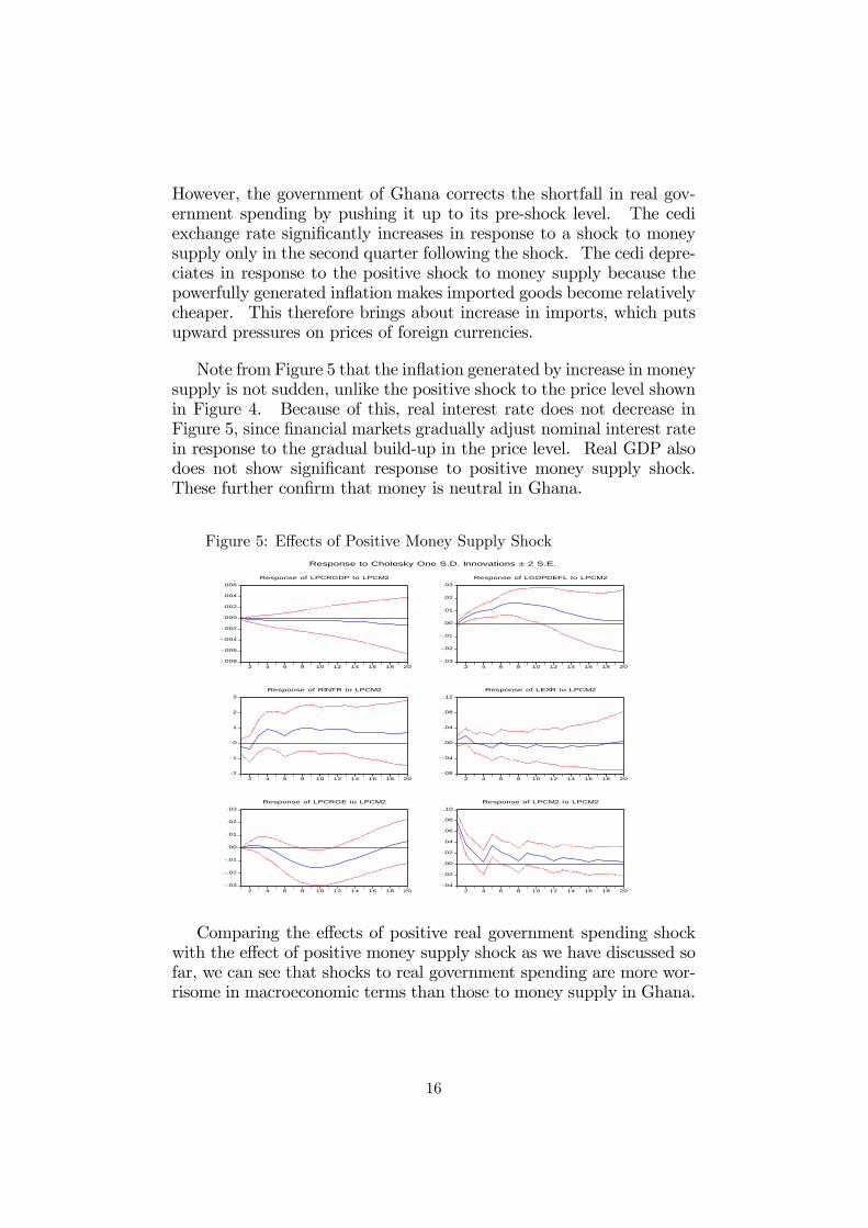
Let us now examine the variance decompositions of real output, theprice level, the exchange rate of the cedi and real interest rate. Thiswill enable us to understand the extent to which variations in thesevariables are accounted for by innovation in government spending (andthose of the other variables). Tables 3a to 3d respectively presents thevariance decompositions of real GDP, the price level, the cedi exchangerate and real interest rate for the �rst 10 quarters as well as 15th and20th quarters.

Table 3a: Variance Decomposition of LPCRGDP

Quarter LPCRGDP LGDPDEFL RINTR LEXR LPCRGE LPCM21 87.85 0.90 1.03 5.71 4.35 0.1592 78.44 0.33 2.91 13.98 3.61 0.743 73.45 0.14 5.56 17.21 2.70 0.954 70.53 0.08 7.16 19.34 1.70 1.195 67.22 0.11 9.03 20.94 1.15 1.566 63.62 0.25 11.15 22.43 0.88 1.697 60.22 0.47 14.87 23.75 0.76 1.688 57.32 0.67 14.87 24.82 0.72 1.609 55.16 0.80 16.39 25.45 0.71 1.5010 53.71 0.82 17.66 25.72 0.70 1.3815 52.39 0.47 20.54 24.88 0.53 1.1820 52.11 0.25 21.35 24.11 0.39 1.78

19

Table 3b: Variance Decomposition of LGDPDEFL

Period LPCRGDP LGDPDEFL RINTR LEXR LPCRGE LPCM21 0.00 94.93 0.00 0.00 4.98 0.092 0.04 80.57 3.23 0.33 3.44 12.383 0.20 63.77 9.12 0.18 1.96 24.774 1.58 49.24 14.60 0.19 1.23 33.175 4.64 40.52 15.46 1.70 0.92 36.756 7.55 33.18 13.34 3.63 1.34 40.967 9.81 27.49 11.18 5.67 3.17 42.688 11.14 23.19 9.73 7.17 5.80 42.979 11.85 19.99 8.76 8.87 8.67 41.8610 12.05 17.19 8.10 10.41 11.50 40.7415 14.69 9.59 10.48 17.06 19.06 29.1120 25.93 6.35 16.23 19.16 14.00 18.32

Figure 3c: Variance Decomposition of LEXR


Figure 3d: Variance Decomposition of RINTR


20

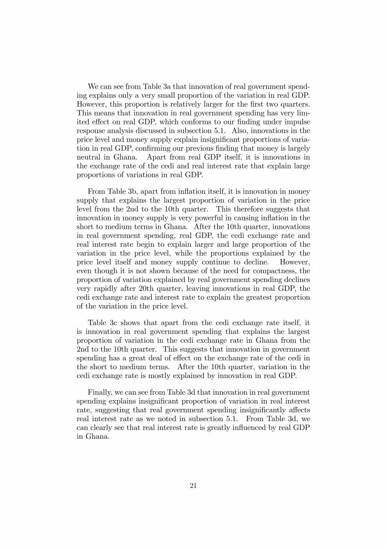
We can see from Table 3a that innovation of real government spend-ing explains only a very small proportion of the variation in real GDP.However, this proportion is relatively larger for the �rst two quarters.This means that innovation in real government spending has very lim-ited e¤ect on real GDP, which conforms to our �nding under impulseresponse analysis discussed in subsection 5.1. Also, innovations in theprice level and money supply explain insigni�cant proportions of varia-tion in real GDP, con�rming our previous �nding that money is largelyneutral in Ghana. Apart from real GDP itself, it is innovations inthe exchange rate of the cedi and real interest rate that explain largeproportions of variations in real GDP.

From Table 3b, apart from in�ation itself, it is innovation in moneysupply that explains the largest proportion of variation in the pricelevel from the 2nd to the 10th quarter. This therefore suggests thatinnovation in money supply is very powerful in causing in�ation in theshort to medium terms in Ghana. After the 10th quarter, innovationsin real government spending, real GDP, the cedi exchange rate andreal interest rate begin to explain larger and large proportion of thevariation in the price level, while the proportions explained by theprice level itself and money supply continue to decline. However,even though it is not shown because of the need for compactness, theproportion of variation explained by real government spending declinesvery rapidly after 20th quarter, leaving innovations in real GDP, thecedi exchange rate and interest rate to explain the greatest proportionof the variation in the price level.

Table 3c shows that apart from the cedi exchange rate itself, itis innovation in real government spending that explains the largestproportion of variation in the cedi exchange rate in Ghana from the2nd to the 10th quarter. This suggests that innovation in governmentspending has a great deal of e¤ect on the exchange rate of the cedi inthe short to medium terms. After the 10th quarter, variation in thecedi exchange rate is mostly explained by innovation in real GDP.

Finally, we can see from Table 3d that innovation in real governmentspending explains insigni�cant proportion of variation in real interestrate, suggesting that real government spending insigni�cantly a¤ectsreal interest rate as we noted in subsection 5.1. From Table 3d, wecan clearly see that real interest rate is greatly in�uenced by real GDPin Ghana.

21

6 Disaggregating Real Government Spending into Capital andConsumption Expenditures

So far, we have treated real government spending as a single vari-able. Let us now disaggregate it into two components: real governmentcapital spending (represented by LPCRGKE = log of per-capita realgovernment expenditure) and real government consumption spending(represented by LPCRGCE = log of per-capita real government con-sumption expenditure). Real government capital spending has greaterpotential to stimulate real GDP because it expands the production ca-pacity of the economy. However, it takes a long time for the economyto realize the bene�ts from many of these government capital outlays.An example is investment in education. Additionally, the bene�ts frommost of these capital outlays by the government are realized over a longstretch of time. Because of these factors, quarterly or even yearly mar-ginal bene�ts from a shock in real government capital spending maybe very small.

Figure 8a and Figure 8b respectively show the impulse-responsefunctions of one standard deviation positive shocks to real governmentconsumption spending and real government investment spending.

Fig. 8a: E¤ects of a Positive Real Gov�t Fig. 8b: E¤ects of a Positive Real Gov.Cons. Spending Shock Capital Spending Shock

.006

.004

.002

.000

.002

2 4 6 8 10 12 14 16 18 20

Response of LPCRGDP to LPCRGCE

.01

.00

.01

.02

.03

.04

.05

2 4 6 8 10 12 14 16 18 20

Response of LGDPDEFL to LPCRGCE

2

1

0

1

2

3

4

2 4 6 8 10 12 14 16 18 20

Response of RINTR to LPCRGCE

.04

.00

.04

.08

.12

.16

2 4 6 8 10 12 14 16 18 20

Response of LEXR to LPCRGCE

.04

.00

.04

.08

2 4 6 8 10 12 14 16 18 20

Response of LPCRGKE to LPCRGCE

.06

.04

.02

.00

.02

.04

.06

2 4 6 8 10 12 14 16 18 20

Response of LPCRGCE to LPCRGCE

.03

.02

.01

.00

.01

.02

.03

.04

.05

2 4 6 8 10 12 14 16 18 20

Response of LPCM2 to LPCRGCE


.004

.003

.002

.001

.000

.001

.002

.003

2 4 6 8 10 12 14 16 18 20

Response of LPCRGDP to LPCRGKE

.03

.02

.01

.00

.01

.02

2 4 6 8 10 12 14 16 18 20

Response of LGDPDEFL to LPCRGKE

3

2

1

0

1

2

3

2 4 6 8 10 12 14 16 18 20

Response of RINTR to LPCRGKE

.04

.00

.04

.08

2 4 6 8 10 12 14 16 18 20

Response of LEXR to LPCRGKE

.04

.02

.00

.02

.04

.06

.08

2 4 6 8 10 12 14 16 18 20

Response of LPCRGKE to LPCRGKE

.04

.03

.02

.01

.00

.01

.02

.03

2 4 6 8 10 12 14 16 18 20

Response of LPCRGCE to LPCRGKE

.03

.02

.01

.00

.01

.02

.03

2 4 6 8 10 12 14 16 18 20

Response of LPCM2 to LPCRGKE


In both Figure 8a and Figure 8b, like a positive shock to total realgovernment spending as we saw in section 5, positive shocks to realgovernment consumption and capital expenditures generate signi�cant

22

but small positive response from real GDP during the �rst quarter.Even though the cedi exchange rate shows some upward movementfrom the time of a positive shock to real government capital expendi-ture to the 11th quarter, it is statistically signi�cant only in the thirdquarter. Thus, depreciation of the cedi that follows a shock to realgovernment capital expenditure is less persistent. However, a shockto real government consumption expenditure signi�cantly and persis-tently brings about depreciation of the cedi. As a result of this, unlikereal capital spending shock that has no signi�cant e¤ect on real outputafter the �rst quarter, real government consumption spending shocksigni�cantly contracts real GDP from the 6th quarter to the 10th quar-ter. In fact, the depreciation of the cedi resulting from a shock to justreal government consumption expenditure is more persistent than theone that results from a shock to total government expenditure. Thisis because, unlike total spending shock, the upward movement in theexchange rate of the cedi following a shock to just real governmentconsumption expenditure as shown in Figure 8a does not return to itspre-shock level for the 20 quarters allowed in the graph, and it is sta-tistically signi�cant during both the �rst third and the last third of the20-quarter period. It is interesting to note that it is real governmentcapital spending component that is the cause of the less persistent na-ture of the depreciation of the cedi that follows a positive shock tototal government spending. Therefore, it is the real capital expendi-ture component that makes a shock to total real government spendingnot signi�cantly contract real output.

Another interesting e¤ects depicted in Figure 8a and Figure 8b arethat a positive shock to real government capital expenditure has noe¤ects on money supply and the price level, while a positive shock toreal government consumption expenditure signi�cantly increases moneysupply and the price level. A reason why a shock to real capitalspending of the government has no e¤ect on money supply and theprice level in Ghana is that, historically, increases in government capitalexpenditure are largely foreign �nanced. By �nancing increases incapital spending externally, the government does not borrow form theBank of Ghana to increase money supply (M2) to cause in�ation.

7 Policy Implications

Based on the �ndings in this study, we can derive the followingpolicy implications for Ghana:

1. Government spending increases, especially those �nanced throughborrowing, should be put under control in Ghana because, through the

23

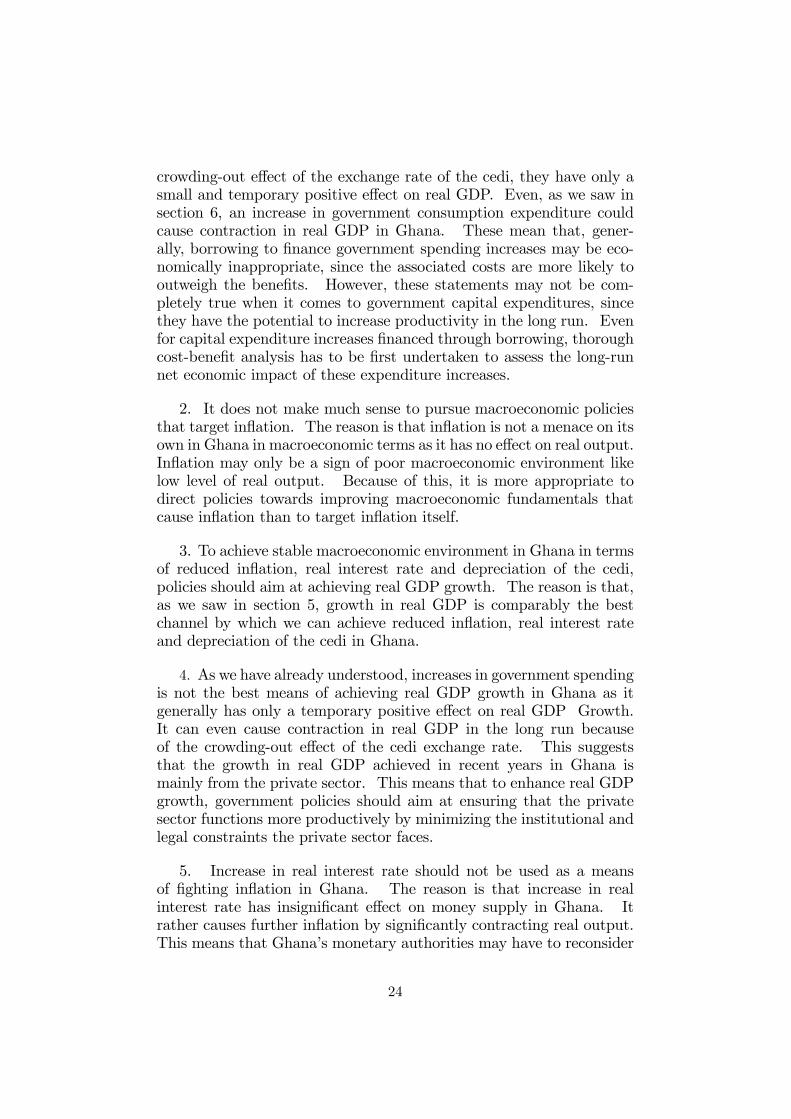
crowding-out e¤ect of the exchange rate of the cedi, they have only asmall and temporary positive e¤ect on real GDP. Even, as we saw insection 6, an increase in government consumption expenditure couldcause contraction in real GDP in Ghana. These mean that, gener-ally, borrowing to �nance government spending increases may be eco-nomically inappropriate, since the associated costs are more likely tooutweigh the bene�ts. However, these statements may not be com-pletely true when it comes to government capital expenditures, sincethey have the potential to increase productivity in the long run. Evenfor capital expenditure increases �nanced through borrowing, thoroughcost-bene�t analysis has to be �rst undertaken to assess the long-runnet economic impact of these expenditure increases.

2. It does not make much sense to pursue macroeconomic policiesthat target in�ation. The reason is that in�ation is not a menace on itsown in Ghana in macroeconomic terms as it has no e¤ect on real output.In�ation may only be a sign of poor macroeconomic environment likelow level of real output. Because of this, it is more appropriate todirect policies towards improving macroeconomic fundamentals thatcause in�ation than to target in�ation itself.

3. To achieve stable macroeconomic environment in Ghana in termsof reduced in�ation, real interest rate and depreciation of the cedi,policies should aim at achieving real GDP growth. The reason is that,as we saw in section 5, growth in real GDP is comparably the bestchannel by which we can achieve reduced in�ation, real interest rateand depreciation of the cedi in Ghana.

4. As we have already understood, increases in government spendingis not the best means of achieving real GDP growth in Ghana as itgenerally has only a temporary positive e¤ect on real GDP Growth.It can even cause contraction in real GDP in the long run becauseof the crowding-out e¤ect of the cedi exchange rate. This suggeststhat the growth in real GDP achieved in recent years in Ghana ismainly from the private sector. This means that to enhance real GDPgrowth, government policies should aim at ensuring that the privatesector functions more productively by minimizing the institutional andlegal constraints the private sector faces.

5. Increase in real interest rate should not be used as a meansof �ghting in�ation in Ghana. The reason is that increase in realinterest rate has insigni�cant e¤ect on money supply in Ghana. Itrather causes further in�ation by signi�cantly contracting real output.This means that Ghana�s monetary authorities may have to reconsider

24

the use of monetary policy instruments that aim at reducing in�ationby causing increases in real interest rate.

8 Conclusion

Using cointegration estimation and innovation analysis, we have em-pirically analyzed the e¤ects, the channels of the e¤ects and the timingof the e¤ects of a shock to government spending on macroeconomicvariables in Ghana. For detailed understanding, we have also consid-ered shocks to other variables. The results show a lot of interesting�ndings. We found that a shock to government spending is not onlyin�ationary but it also causes the cedi to depreciate. As a result ofthe crowding-out e¤ect of the cedi depreciation, the signi�cantly posi-tive e¤ect on real GDP is temporary as it is realized only in the �rstquarter that follows the spending shock. We also found that whilepositive shocks to real government consumption and capital expendi-tures positively a¤ect real GDP during the �rst quarter that followsthe shocks, a shock to real government consumption expenditure sig-ni�cantly contracts real output after the �rst quarter because it causesmore persistent depreciation of the cedi.

Furthermore, we found that money is largely neutral in Ghana,implying that shocks to money supply and thus the price level haveinsigni�cant e¤ects on real economic variables. Additionally, we foundthat increase in real interest rate contracts real output and causes in-�ation, while growth in real output is a good, if not the best, means ofachieving macroeconomic stability in Ghana.

Based on these �ndings, the following policy implications were de-rived: 1) Government spending increases should be checked in Ghana.2) To achieve stable macroeconomic environment, it is more appropri-ate to direct policies to accelerate real GDP growth. 3) Governmentpolicies should aim at facilitating the private sector, since real GDPgrowth in Ghana is achieved mostly through the private sector 4)Monetary authorities in Ghana should avoid the use of monetary pol-icy instruments that cause real interest rate to increase, since it is notonly ine¤ective in a¤ecting money supply, it causes further in�ation bycontracting real output.

25

References

Abbey, J.L.S., "A macroeconometric model of the Ghanaian Economy1956 �1969". Economic Bulletin of Ghana (1974)

Amoah, B. and F. W. Loloh, "Causal Linkages between GovernmentRevenue and Expenditure: Evidence from Ghana". Bank of Ghana WorkingPaper Series �WP/BOG-2008/08 (2008)

Amoako, K. Y., "Balance of Payments and Exchange Rate Policy: TheGhanaian Experience". Garland, New York (1980)

Atta-Mensah, J. and M. Bawumia, "A Simple Vector Error CorrectionForecasting Model for Ghana". Bank of Ghana Working Paper Series �WP/BOG-2003/01 (2003)

Bilbiie, F. O., and A. Meier, "What Accounts for the Changes in U.S.Fiscal Policy Transmission?". European Central Bank Working Paper Series�No. 582 (2006)

Choi, W. G., M. B. Devereau, "Asymmetric E¤ects of GovernmentSpending: Does the Level of Real Interest Rates Matter?". IMF WorkingPaper Series �WP/05/7 (2005)

Fatás, A. and I. Mihov, "The E¤ects of Fiscal Policy on Consumptionand Employment: Theory and Evidence". mimeo, INSEAD (2001)

Ghartey, E. E., "Macroeconomic instability and in�ationary �nancing inGhana". Economic Modelling (2001)

Ghartey, E. E., "Monetary Dynamics in Ghana: Evidence from Cointe-gration, Error Correction Modelling, and Exogeneity". Journal of Develop-ment Economics (1998)

Ghartey, E. E., "Devaluation as a balance of payments corrective mea-sure in developing countries: a study relating to Ghana". Applied Economics(1987)

Ghartey, E. E., and U.L.G. Rao, "A Short-run Forecasting Model ofGhana". Economic Modelling (1990)

Ghatak, A. "Vector Autoregression Modelling and Forecasting Growthof South Korea". Journal of Applied Statistics (1998)

Kandil, M. "On the Transmission Mechanism of Policy Shock in Devel-oping Countries". Oxford Development Studies (2006)

Leith, J.C., "Foreign Trade Regimes and Economic Development: Ghana".Bureau of Economic Research, New York (1974)

Perotti, R. "Estimating the E¤ects of Fiscal Policy in OECD Countries".Centre for Economic Policy Research Discussion Paper Series (2005)

26

The Transmission Mechanism of Governemnt Spending in Ghana: Empirical Analysis and Policy...

Documents

Transcript of The Transmission Mechanism of Governemnt Spending in Ghana: Empirical Analysis and Policy...