The housing market and consumer spending

The Housing Market and Consumer Spending

ALAN CARRUTH and ANDREW HENLEY*

1. INTRODUCTION

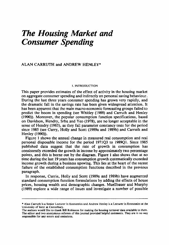
This paper provides estimates of the effect of activity in the housing market on aggregate consumer spending and indirectly on personal saving behaviour . During the last three years consumer spending has grown very rapidly, and the dramatic fall in the savings rate has been given widespread attention. It has been apparent that the main macro-economic forecasting groups failed to predict the boom in spending (see Whitley (1989) and Carruth and Henley (1 990)). Moreover, the popular consumption function specifications, based on Davidson, Hendry, Srba and Yeo (1978), are no longer acceptable in the sense of Hendry (1983), as they fail parameter constancy tests for the period since 1985 (see Curry, Holly and Scott (1989a and 1989b) and Carruth and Henley (1 990)).

Figure 1 shows the annual change in measured real consumption and real personal disposable income for the period 197143 to 198941. Since 1985 published data suggest that the rate of growth in consumption has consistently exceeded the growth in income by approximately two percentage points, and this is borne out by the diagram. Figure 1 also shows that at no time during the last 19 years has consumption growth systematically exceeded income growth during a business upswing. This lies at the heart of the recent failure of the established consumption functions described in the previous paragraph.

In response, Currie, Holly and Scott (1989a and 1989b) have augmented standard consumption function formulations by adding the effects of house prices, housing wealth and demographic changes. Muellbauer and Murphy (1989) explore a wide range of issues and investigate a number of possible

Alan Carruth is a Senior Lecturer in Economics and Andrew Henley is a Lecturer in Economics at the University of Kent at Canterbury. The authors would like to thank Bill Robinson for making the housing turnover data available to them. The editor and two anonymous referees of this journal provided helpful comments. They are in no way responsible for any errors and omissions.

Fiscal Studies

FIGURE I

1 l l l l l l l l l l l l , l , J , ~ 1 1973 1975 1977 1979 1981 1983 1985 1987 1989

mis-specifications of aggregate consumption functions: (i) rising wealth to income ratios; (ii) financial liberalisation; (iii) reduced uncertainty with respect to real income growth; (iv) demographic changes involving an increase in the proportion of the population with low savings rates; (v) a fall in institutional savings rates; (vi) tax cut promises raising expected incomes; (vii) cuts in publicly produced alternatives to private consumption like education and health; and (viii) mismeasurement in national accounts data. Under financial liberalisation they examine the important role of the housing market. Two distinguishing features of their approach are (i) the way price and interest rate effects and credit constraints are integrated into a general empirical model of consumer spending behaviour and (ii) the encompassing implications of their preferred empirical model.

Lee and Robinson (1990) have studied the impact of the housing market on savings, without pursuing a fully developed empirical model of aggregate consumer spending. They emphasise the phenomenon of equity withdrawal arising from the way house purchases are financed - roughly stated as the difference between lending for house purchase and actual investment in new housing. The authors identify four types of equity withdrawal: ‘last time sellers of owner occupied houses; sellers of formerly rented properties; moving owner occupiers borrowing more than the difference between the price of their old house and the new; and those trading down to a cheaper house’ (Lee and Robinson, 1990, p. 40). However, it must be noted that these

28


-6

possibilities for withdrawal do not presuppose that the money is automatically spent, as investment in other financial assets will be part of the choice process.'

Our suggestion is that, in the context of aggregate consumption functions, the concept of housing equity withdrawal (HEW) might usefully be linked to the old problem of how we measure income; see Hicks (1946, p. 179) for a general discussion. Therefore, this paper integrates the concept of HEW into an aggregate consumption function model, and directly estimates the effect of HEW on personal disposable income. From this framework we can calculate an expost measure of 'adjusted' income, to be distinguished from the measure of disposable income published by the CSO, which we shall call 'measured' income. Our econometric analysis follows closely that of Hendry and von Ungern-Sternberg (HUS) (1981), who adopted such an approach to adjust measured income to take account of inflation effects on liquid asset holdings. Therefore, our approach complements the work of Lee and Robinson (1990) and Muellbauer and Murphy (1989).

Our measure of adjusted income including HEW, which is explained below, is shown in Figure 2. It provides a sharp contrast with Figure 1. Since

- I I Y I1

- I I l l l 1 1 I 1 1 1 1 ~ ~ 1 1 1 1 1

FIGURE 2

Annual Change in Measured Real Consumption and Adjusted Real Personal Disposable Income, 197143 to 1989Q1

l*[ :I 10

A I \ I \ I I

-2 O m " : I I \1111;/

I Even though for every seller of a house there must be a buyer, the housing equity withdrawal effect does not net out, because it is linked to the financing of property purchase and credit creation.

29

Fiscal Studies

Adjusted \ - - _

4-

1 1 1 1 1 1 1 1 1 1 1 1 1 1 1 1 1

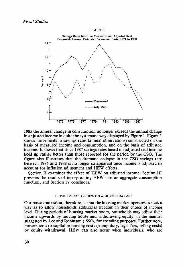
FIGURE 3

Savings Rates based on Measured and Adjusted Real Disposable Income Converted to Annual Basis, 1971 to 1988

1 4 r

1985 the annual change in consumption no longer exceeds the annual change in adjusted income in quite the systematic way displayed by Figure 1. Figure 3 shows movements in savings rates (annual observations) constructed on the basis of measured income and consumption, and on the basis of adjusted income. It shows that since 1987 savings rates based on adjusted real income hold up rather better than those reported for the period by the CSO. The figure also illustrates that the dramatic collapse in the CSO savings rate between 1985 and 1988 is no longer so apparent once income is adjusted to account for inflation adjustment and HEW effects.

Section I1 examines the effect of HEW on adjusted income. Section I11 presents the results of incorporating HEW into an aggregate consumption function, and Section IV concludes.

11. THE IMPACT OF HEW ON ADJUSTED INCOME

Our basic contention, therefore, is that the housing market operates in such a way as to allow households additional freedom in their choice of income level. During periods of housing market boom, households may adjust their income upwards by moving house and withdrawing equity, in the manner suggested by Lee and Robinson (1990), for spending purposes. Furthermore, movers tend to capitalise moving costs (stamp duty, legal fees, selling costs) by equity withdrawal. HEW can also occur when individuals, who are

30


already themselves owner-occupiers, sell property left by recently deceased relatives and spend all or part of the net proceeds. This latter effect may have been growing in importance recently as people have begun to inherit property bought by parents during the period of owner-occupation growth shortly after the Second World War. There has also been widespread publicity about individuals taking second mortgages on existing property because of favourable borrowing rates, and then using the money for spending.

The HEW process, we would argue, may not be symmetric in upswings and downswings in the housing market. During downswings when desired moves are arrested by low housing turnover, we do not tend to observe housing equity growth through households accelerating the repayment of housing loans. Such repayment might occur if households (with repayment mortgages) fail, due to inertia, to revise downwards regular mortgage repayments when interest rates fall. However, during periods of low housing turnover it is more likely that interest rates are rising, and in any case mortgages are increasingly of the endowment type. Furthermore, if people cannot move then they may save in anticipation of financing a move once the market revives. But recent experience would suggest that such saving will generate a much lower rate of return than investment in property, not least because of the fiscal incentives in favour of owner-occupation investment.

Equity withdrawal through re-mortgaging and second mortgaging may be unrelated directly to housing market activity. But such forms of withdrawal may be conditioned by the level of interest rates, and so indirectly correlated with housing turnover. This suggests an asymmetric modelling approach, with personal incomes being revised upwards to take account of HEW during housing market upswings, but possibly not downwards during housing market recessions. One possible way of formalising HEW is to posit that HEW is equal to a fixed proportion, 6, of liquid housing wealth. The liquidity of housing wealth is governed by the state of the housing market, and depends essentially upon prices and turnover. Therefore real HEW during any time period is given by:

H E W = 6 T W h (1) where T is the proportion of the stock of owner-occupied dwellings bought and sold during the period in question, and Wh is the real value of private housing assets. Incorporating this into the HUS (1981) approach to consumers’ expenditure modelling we can obtain a measure of adjusted income, Y*, as follows:

(2) where Y is measured real personal disposable income. /3’W is the HUS (198 1) term to capture inflation-induced ‘topping-up’ of asset holdings. The justification for the inclusion of this term is in arguing that households will devote some increasing proportion of actual incomes to maintaining real asset holdings in times of rising inflation. p is inflation, W total personal

Y* = Y - f l p W + D 6 T wh

31

Fiscal Studies

sector real assets and /3 a scale parameter. fl captures the extent to which consumers are able to compensate for the erosion of their assets.2 If /3 equals 1 then consumers fully restore the real value of assets from their current incomes.

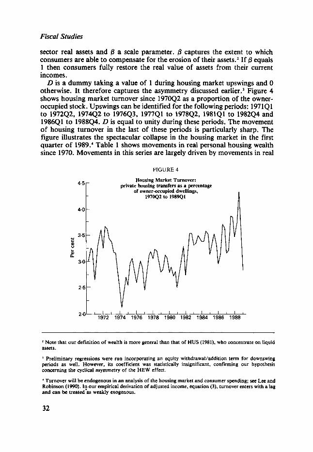
D is a dummy taking a value of 1 during housing market upswings and 0 otherwise. It therefore captures the asymmetry discussed earlier.3 Figure 4 shows housing market turnover since 197042 as a proportion of the owner- occupied stock. Upswings can be identified for the following periods: 197141 to 197242, 197442 to 197643, 197741 to 197842, 198141 to 198244 and 198641 to 198844. D is equal to unity during these periods. The movement of housing turnover in the last of these periods is particularly sharp. The figure illustrates the spectacular collapse in the housing market in the first quarter of 1989.' Table 1 shows movements in real personal housing wealth since 1970. Movements in this series are largely driven by movements in real

FIGURE 4

Housing Market Turnover: private housing transfers as a percentage

of owner-occupied dwellings, 197042 to 198941

4.0 A

"O ' ' 1Ei72 19174 19176 ' l h 8 ' d 8 0 19182 I 1d84 1&6 ' 1d88 '

* Note that our definition of wealth is more general than that of HUS (1981), who concentrate on liquid assets.

Preliminary regressions were run incorporating an equity WithdrawaVaddition term for downswing periods as well. However, its coefficient was statistically insignificant, confirming our hypothesis concerning the cyclical asymmetry of the HEW effect.

' Turnover will be endogenous in an analysis of the housing market and consumer spending; see Lee and Robinson (1990). I? our empirical derivation of adjusted income, equation (9, turnover enters with a lag and can be treated as weakly exogenous.

32


TABLE 1

Net Equity Value of Housing

f billion (1985 prices)

1970 1972 I974 1976 1978 1980 1982 1984 1986 1988

207.9 293.8 341.4 286.9 311.0 382.3 331.1 369.9 446.6 655.5

Note: Calculated as (average house price) x (stock of owner-occupied dwellings) - (outstanding mortgages).

average house prices, and the rapid growth in housing wealth since 1984 is clearly illustrated. This growth, coupled with the housing turnover boom of 1986 to 1988, suggests the potential for a huge growth in HEW fuelling the spending boom of that period. Furthermore, relatively stable consumer prices meant that inflation-induced wealth ‘topping-up’ will have been much reduced.

Introduction of this revised income definition into an error-correction, HUS-type consumption function introduces non-linearities, since it involves the replacement of Y with Y*. Equation (2) is incorporated empirically as:

(3) Y f = Yr - flfitWr-1 + Dt-16Tt-I Whf-1

where 91 = 0.25 (PI - pr-4) and p is the consumers’ expenditure deflator.

111. RESULTS

Table 2 presents estimates of a HUS-type consumption function specification for the period 197144 to 198941, incorporating the HEW extension to the definition of ‘adjusted’ i n ~ o m e . ~ Y* was then calculated using these coefficient estimates and, following HUS, the linear model re-estimated by Ordinary Least Squares (OLS) on PC-GIVE to obtain the full set of

’ The results for j? and 6 were obtained by maximum likelihood estimation of the general non-linear model which included the Y* equation and the empirical model reported in Carruth and Henley (1990).

33

Fiscal Studies

TABLE 2

Consumption Function Regression Results

Dependent variable: A4c Sample:

P

6

(W-Y*)r-r

A a 7 3 0 1

A,D7902

Constant

QI

Q2

Q3

R’ SER AR(5) Chi’ ARCH(4) Chi’ Normality Chi* Het. F(19,26(38)) Res. F( 1,45(57)) Forecast Chiz Chow F(12,46) Dynamic forecast, MSAPE

Total Total 7144-8641, 7144-8941 12 forecasts

0.104 (2.64) 0.089

(1.83) 0.264 (4.00) 0.398 (7.26) - 0.264

( - 3.05) 0.025

(1.51) 0.095

(1.56) - 0.021

(- 1.70) 0.032

(4.04) 0.044

(5.43) - 0.049

( - 0.86) 0.008

(1.927) 0.017 (2.90) 0.003

(0.75)

0.892 1.069% 5.656 7.003 0.848 0.365 0.447 1.41 0.92 0.012

0.121 (3.07) 0.122

(3.22) 0.308 (5.02) 0.379 (7.89) - 0.267

( - 3.50) 0.037 (3.38) 0.084

(1.85) - 0.019

( - 1.74) 0.033

(4.24) 0.045

(5.69) - 0.084

( - 2.06) 0.010 (2.47) 0.018 (3.22) 0.003

(0.76)

0.895 1.052% 7.433 4.878 0.261 0.442 0.594 - - -

Note: Estimates of fl and 8 obtained by non-linear maximum likelihood estimation, using TSP 4.1. These were imposed to allow OLS estimation of the linear HUS model to provide comprehensive diagnostics, using PC-GIVE 6.0. The dynamic forecast mean sum absolute prediction error was obtained using Microfit, by Pesaran and Pesaran (1987).

34


diagnostic information. The additional explanatory variables are as follows:

r : real post-tax long-term rate of interest; 07301 : dummy variable to capture anticipation effect of

07902 : dummy variable to capture anticipation effect of

Q1, Q2, Q3 : seasonal intercept terms.

1973 Budget changes;

1979 Conservative Budget changes;

Estimates are presented for total consumer spending. Results for non- durable spending (not reported) are very similar. Lower case letters indicate logs. The rationale for the dynamic specification reported is as follows. The annual growth in consumer spending in any quarter is determined by last quarter’s growth (A4ct-,), the annual growth in adjusted income (A,y*) and the previous quarter’s growth in personal wealth (Awt-,). These change variables are capturing the dynamic equilibrium adjustment of consumption. The levels terms describe the steady state, and in error-correction form capture the disequilibrium adjustment, so that consumption is modified by the feedback from the logarithm of last year’s adjusted average propensity to consume, (c - Y * ) ~ - ~ , the logarithm of last year’s wealth-adjusted income ratio, (w-y*)t-*, and last quarter’s real long-term rate of interest, rr-l.

Table 2 shows that the HEW parameter, 6, is estimated to be 9 per cent for the period up to 198641. In the full sai1ple results it rises to 11 or 12 per cent, so that in the latest housing boom the HEW effect has become more pronounced. The 6 parameter shows that on average between 10 and 12 per cent of the adjustment necessary to keep real asset holdings constant in value is made.6 The model adequacy tests are all satisfactory, in particular the Chow statistic does not indicate any breakdown in the relationship. The within-sample static forecast test is a considerable improvement on th-e result reported in Carruth and Henley (1990) (equation 2, forecast Chi2 = 3.42) for a HUS-type specification which neglected the HEW effect. The dynamic forecast test suggests a prediction error of roughly 1 percentage point on average (consumer spending is measured as annual percentage growth). There was no tendency for the actual and predicted values to diverge over the dynamic forecast period, 198642 to 198941. In fact the smallest prediction error was for the period 198941.’

Our results serve to illustrate the growing importance of housing market

Note that 0 is essentially a scale parameter, and so our estimate differs from HUS (B = 0.5), because we have used total wealth whereas HUS use liquid assets.

’ Consideration of an ex post, out-of-sample simulation analysis in the context of macro-econometric forecasting models is beyond the scope of this paper. However, it will be interesting to see to what extent the reappraisal of aggregate consumption functions, described in this paper, influences the macroeconomic forecasting agencies. It is certainly our contention that the HEW phenomenon is worthy of consideration.

35

Fiscal Studies

activity in explaining consumer spending in the late 1980s. Figure 4 shows that since 1982 up to the eve of the housing market collapse in 1989 the proportion of houses traded to the total owner-occupied housing stock rose from 12 to over 15 per cent per annum. 15 per cent of the €655 billion worth of housing equity in 1988 (Table 1) gives a total traded volume of equity of nearly €100 billion. So, households enjoyed the ability to withdraw up to 12 per cent (estimate of 6 from Table 2) of this f 100 billion to boost current incomes for spending purposes; in other words, an equity withdrawal of f 12 billion at 1985 prices. In fact in 1988 our adjusted income measure for the year exceeds measured personal disposable income by f 4 billion at 1985 prices, implying a mitigating wealth ‘topping-up’ effect of €8 billion. If inflation had not begun to rise by 1988 then equity withdrawal might have had a far more severe effect on consumer incomes and therefore spending.

1V. CONCLUSION

This paper has tried to suggest one way that the analysis of housing equity withdrawal by Lee and Robinson (1990) could be incorporated into an aggregate consumption function using the approach suggested by Hendry and von Ungern-Sternberg (1981). Table 2 shows that the resulting empirical model performs well and satisfies a conventional set of adequacy criteria. As such it complements the extensive research by Muellbauer and Murphy (1989) into the breakdown of consumption relationships since 1985. Our estimate of the equity withdrawal effect means that in 1988 households had the choice of spending an additional El2 billion over and above their measured disposable income. This could have added up to 4 per cent to consumer spending in a year when it actually registered an astonishing (and unpredicted) 7 per cent growth rate.

Somewhat speculatively, our results suggest that the dramatic termination of the housing boom, in response to the sharp tightening in monetary policy, combined with rising inflation should have a considerable dampening effect on consumer spending. At the time of writing, this is becoming apparent. Nevertheless this dampening effect could easily be eroded by a restoration of activity in the housing market and by the effect on housing turnover and prices of sustained real wage growth. Our estimates of the effects of HEW on ‘adjusted income’ show that the operation of the housing market has the potential to generate a high level of inflationary pressure. The question of the impact of HEW may constitute an important issue worthy of future consideration by policy-makers (see Spencer (1990)).

APPENDIX: DATA DEFINITIONS AND SOURCES

Consumers’ expenditure, total and non-durables, constant 1985 prices (CSO Databank).

36


Personal disposable income, constant 1985 prices (CSO Databank). Personal sector wealth: net personal financial wealth outstanding (CSO Databank), adding back in outstanding mortgages, in current prices, deflated by the implicit consumers’ expenditure deflator (CSO Databank) plus net housing wealth. Outstanding mortgages: net advances for house purchase, current prices (CSO Databank) cumulated using 198844 figure for outstanding mortgages, obtained from Department of Environment, Housing and Construction Statistics, as a bench-mark. Net housing wealth: average house price, current prices (CSO Databank) times UK stock of owner-occupied housing (Housing and Construction Statistics) less outstanding mortgages, deflated by implicit consumers’ expenditure deflator. Real post-tax long-term rate of interest: gross redemption percentage yield on 20-year British Government Stock (CSO Databank) multiplied by 1 minus the basic rate of income tax less the annual percentage growth in the implicit consumers’ expenditure deflator. Housing turnover rate: number of ‘particulars delivered’ to the Inland Revenue for stamp duty assessment’ divided by stock of owner-occupied dwellings (kindly provided by Bill Robinson).

REFERENCES

Carruth, A. and Henley, A. (1990), ‘Can existing consumption functions forecast consumer

Currie, D.. Holly, S. and Scott, A. (1989a), ‘Macroeconomic viewpoint: savings and the

-, - and - (1989b), ‘Savings, demography, and interest rates’, LBS Discussion Paper no.

Davidson. J., Hendry, D., Srba, F. and Yeo, S. (1978), ‘Econometric modelling of the aggregate time series relationship between consumers’ expenditure and income in the UK’, Economic Journal, vol. 80, pp. 661-692.

Hendry, D. (1983). ‘Econometric modelling: the consumption function in retrospect’, Scottish Journal of Political Economy, vol. 30, pp. 193-220.

- and von Ungern-Sternberg, T. (1981), ‘Liquidity and inflation effects on consumers’ expenditure’, in A. S . Deaton (ed.), Essays on the Theory and Measurement of Consumers’ Behaviour, Cambridge: Cambridge University Press.

spending in the late 1980s?’, Odord Bulletin, May.

Budget’, Economic Outlook, vol. 13, pp. 16-23.

01-89.

Hicks, J. R. (1946), Value and Capital, second edition, Oxford: Clarendon Press. Lee, C. and Robinson, P. W. (1990), ‘The fall in the savings ratio: the role of housing’, Fiscal

Muellbauer, J. and Murphy, A. (1989), ‘Why has UK personal saving collapsed?’, Research Studies. vol. 11, no. 1, pp. 36-52.

Paper, Credit Suisse First Boston, July.

The Inland Revenue receives particulars of all house transfers, regardless of whether or not they fall below the Stamp Duty threshold.

37

Fiscal Studies

Pesaran, M. H. and Pesaran, B. (1987), Microfit User Manual, Oxford: Oxford University

Spencer, P . (1990), EMS: How to Prepare Britain for Full Membership, Shearson Lehmann

Whitley, J . D. (1989), ‘Consumer spending in the UK quarterly models’, paper presented to

Press.

Hutton.

ESRC Macroeconomic Modelling Seminar, May.

The housing market and consumer spending

Documents

Transcript of The housing market and consumer spending