Time Series Analysis Nonlinear Cointegration and Nonlinear Error Correction: Record Counting...

Communications in Statistics—Simulation and Computation®, 35: 939–956, 2006Copyright © Taylor & Francis Group, LLCISSN: 0361-0918 print/1532-4141 onlineDOI: 10.1080/03610910600880351

Time Series Analysis

Nonlinear Cointegration and Nonlinear ErrorCorrection: Record Counting Cointegration Tests

ALVARO ESCRIBANO1, ANA E. SIPOLS2, ANDFELIPE APARICIO3

1Department of Economics, Universidad Carlos III de Madrid, Spain2Department of Statistics, Universidad Rey Juan Carlos, Madrid, Spain3Department Statistics, Universidad Carlos III de Madrid, Spain

In this article we propose a record counting cointegration (RCC) test that is robustto nonlinearities and certain types of structural breaks. The RCC test is based on thesynchronicity property of the jumps (new records) of cointegrated series, countingthe number of jumps that simultaneously occur in both series. We obtain the rate ofconvergence of the RCC statistics under the null and alternative hypothesis. Sincethe asymptotic distribution of RCC under the null hypothesis of a unit root dependson the short-run dependence of the cointegrated series, we propose a small samplecorrection and show by Monte Carlo simulation techniques their excellent smallsample behaviour. Finally, we apply our new cointegration test statistic to severalfinancial and macroeconomic time series that have certain structural breaks andnonlinearities.

Keywords Cointegration; Counting statistics; Jumps; Nonlinearity; Ranges;Robustness; Small sample corrections; Structural breaks; Unit roots tests.

Mathematics Subject Classification 37M10; 62M10.

1. Introduction

Granger (1981) introduced the concept of cointegration and with the contribution ofEngle and Granger (1987) and Johansen (1991) this concept has achieved immensepopularity among econometricians and applied economists. Only a few recentpapers have been dedicated to the simultaneous consideration of nonstationarityand nonlinearity, even though many people agree that those are likely characteristicsof many macroeconomic and financial economic relationships. Granger (1995)discussed the concepts of long-range dependence in mean and extended memorythat generalize the linear concept of integration, I�1�, to a nonlinear framework.

Received February 19, 2005; Accepted May 3, 2005Address correspondence to Ana E. Sipols, Department of Statistics, Universidad

Rey Juan Carlos, Calle Tulipán S/N 28933 Mosteles, Madrid, Spain; E-mail:[email protected]

939

Downloaded By: [University Carlos III of Madrid] At: 12:17 12 May 2009

1

Referencia bibliográfica

Published in:Communications in Statistics. 2006, vol. 35, nº 4. p. 939-956, ISSN 1532-4141 Taylor & Francis

940 Escribano et al.

On the other hand, there are interesting empirical macroeconomic applicationswhere nonlinearity has been found in a nonstationary context and therefore, thereis a need to justify those results econometrically.

Most unit root tests, like those of Dickey and Fuller (1979) or Phillips andPerron (1988), are not robust to outliers, Franses and Haldrup (1994); nor tostructural breaks, Perron (1990); nor to nonlinear transformations, Granger andHallman (1991) and Aparicio et al. (2006a). Therefore, tests for noncointegrationbased on the augmented Dickey and Fuller (ADF) test applied to the residuals ofthe cointegrating relationship, Engle and Granger (1987), have size distortions andlosses in power. Aparicio et al. (2004, 2006a) analyzed the asymptotic properties ofa new range unit root (RUR) test and provide evidence of their nice behavior byMonte Carlo simulation of nonlinearities and structural breaks and by someempirical applications.

In this article we analyzed the properties of a RCC test that is robust tomonotonic nonlinear transformations and structural changes. This testing procedureworks with the ranges, instead of using the actual variables. The range for agiven time t is defined as the difference between the cumulative maximum and thecumulative minimum at that time t. The first differences of the ranges are calledthe jumps and they represent the arrival of a new maximum or minimum (newrecord). The RCC test analyzed in this article is based on counting the synchronicityof the jumps (new maximum or minimum) of the cointegrated series. This statisticcounts the number of jumps that simultaneously occur in both series. We comparethe properties of the well-known non cointegration test (see Engle and Granger[EG], 1987), with those of RCC. We show by Monte Carlo simulations how EGdramatically fails in the presence of nonlinearities and structural breaks. These well-known results are general and affect most of the available tests of cointegration ornon-cointegration, like Johansen (1991), etc.

We have considered as empirical applications the prices of gold and silver,analyzed by Escribano and Granger (1998) and the UK money demand from 1878to 2000, analyzed by Escribano (2004). Those data sets were selected because therewas evidence that the series were cointegrated only after explicit treatments ofnonlinearities or structural breaks or both. In this article, however, we find evidenceof cointegration without any previous treatment (prefiltering) of those problems.

2. Analysis Based on Record Counting Cointegration (RCC)

In this section we introduce nonparametric methods to analyze cointegration thatdo not impose restrictions on the functional form relating the variables. Some ofthose procedures are robust to certain types of structural breaks (or level shifts) andmonotonic nonlinear transformations.

Aparicio (1995), Aparicio and Granger (1995), and Aparicio et al. (2006b)propose an alternative nonparametric methodology to test for unit roots. Thebasic idea behind this approach is to count recursively the number of new records(maximum or minimum) in a time series. We expect nonstationary cointegratedseries to have many more new corecords (or synchronous new records) thannoncointegrated series or stationary series. To be more precise we need to introducesome concepts and definitions that are useful in the rest of the article.

Definition 1. Given a time series xt we define the sequence of extremes of xt as thesequence of x1�t = min�x1� � � � � xt� and xt�t = max�x1� � � � � xt�, when t = 1� 2� � � � � n.


2

Record Counting Cointegration Tests 941

Definition 2. Let n be the sample size, the sequence of ranges of xt is defined as

R�x�t = xt�t − x1�t for t = 1� � � � � n� (1)

Definition 3. Given the sequence of ranges we can define the sequence of jumps(new records) as the sequence of first differences of ranges:

�R�x�t = R

�x�t − R

�x�t−1� (2)

The series of new records �R�x�t is positive or zero. When there is a new record

(maximum or minimum) in �x1� � � � � xt�, the first difference of the ranges will bepositive at time t, �R�x�

t > 0. A statistics record was proposed by Aparicio et al.(2006a) for robust unit root testing. When the original series is stationary, with finitevariance, the series of first differences of the ranges are positive at the beginning ofthe sample and the rest is almost a sequence of zeros. On the contrary when theseries are nonstationary I�1� new records appear with positive probability as thesample increases. The key idea relied on the different vanishing rates of the long-run frequency of a new record, n−1∑n

t=1 1��R�x�t > 0�, for an I�1� and an I�0� time

series, in such a way that the normalized long-run frequency of records

J�n�x = n−1/2

n∑t=1

1(�R

�x�t > 0

)(3)

converged in probability to zero under the alternative of stationary, and to anondegenerate positive random variable under the null hypothesis of a unit root. Awell-known result from extremal theory is that the statistical properties of recordsfrom iid sequences of random variables are shared by a wide class of dependentstationary time series (see for instance, Leadbetter and Rootzén, 1988; Lindgren andRootzén, 1988). This prompts the question of whether short-run dependencies andcross-dependencies may have an impact on a record-based test for cointegration.Then, one important alternative model to consider in this context is the case ofdependent random walks.

For plots of the sequence of ranges R�y�t and R

�x�t of Models 1 to 4 below, see

Aparicio et al. (2006b). The following models are useful to motivate the new approachwe are proposing with parameter values equal to � = 0�5, b = 0�6, where et�0, et�1, et�2are standard normal distributions and are mutually independent, Nid(0,1).

Model 1 (Linear cointegration): xt =wt + et�1, yt = �wt + et�2 where wt = wt−1 + et�0.Model 2 (Nonlinear cointegration): xt =wt + et�1� yt = �w2

t + et�2 where wt

= wt−1 +et�0.Model 3 (Independent random walks): xt = xt−1 + et�1, yt = yt−1 + et�2.Model 4 (Random walks with short-run dependence �a �= 0��: �xt = et�1, �yt =

a�xt + et�2.

Figure 1 shows the cross plots of the sequences of new records or first differenceof ranges for the different models. From the cross plot of Fig. 1 it is clearthat dependent but not cointegrated random walks (d) have several new recordssynchronized indicating some small number of corecords. This property will likelyreduce the power of the RCC test if the short-run correlation is high relative to thecointegration relationship. The idea that cointegrated series imply arrivals of highly


3


Figure 1. Cross plots of �R�y�t and �R

�x�t for pairs of series that are (a) linearly cointegrated

(model 1), (b) nonlinearly cointegrated (model 2), (c) independent random walks (model 3),and (d) random walks with short-run dependence (model 4).

synchronized new records suggests the following nonparametric test statistic that wecalled RCC

RCC�n�x�y =

∑nt=1 1

(�R

�x�t > 0

)1(�R

�y�t > 0

)log�n�

� (4)

where the product of the two indicator functions 1��R�x�t > 0�1��R�y�

t > 0� countsthe number of arrivals of new records that are coincident or synchronized(corecords). That is, the RCC counts how many of the total arrivals of the jumpscoincide, relative to the log�n�. Therefore, the convergence rates of the test statisticRC is log�n�.

Theorem 1. Let the processes xt =∑t

i=1 ei�1 and yt =∑t

i=1 ei�2 for t = 1� 2� � � � ��,where ei�1 and ei�2 are independent continuous zero-mean iid sequences with finitevariances and symmetric pdf. Let RCC�n�

x�y be the number of joint records of xt and yt ina sample of size n (4). Then

log�n�−1RCC�n�x�y → 1� (5)

E{RCC�n�

x�y

} = O�log n�� (6)

Var{RCC�n�

x�y

} = O�log n�� (7)


4


Proof. See the Appendix.

2.1. Consistency

If xt and yt are cointegrated, then for some a �= 0 there exists an I�0� sequence tsuch that yt = axt + et�2. Since for large t, xt will dominate et�2, we can write

RCC�n�x�y =

∑nt=1 1

(�R

�x�t > 0

)1(�R

�y�t > 0

)log�n�

�∑n

t=1 1(�R

�x�t > 0

)log�n�

� (8)

But we know from Aparicio et al. (2006a) that∑n

t=1 1��R�x�t > 0� = O�n1/2�.

Thus under the alternative hypothesis of cointegration, the test statistic will satisfy

�log n�−1RCC�n�x�y → �� (9)

2.2. Invariance Against Monotonic Nonlinearities

Monotonic transformations preserve the ordering of the observations in any timeseries, and thus the inter-record times. As a consequence, if we let f�·� and g�·� be amonotonic nonlinear transformations, we must have

RCC�n�

f�x��g�y� = RCC�n�x�y� (10)

More generally, let xt and yt be I�1� time series variables, and let x′t = f�yt�+ t,y′t = g�xt�+ t, where �t�t≥1� �t�t≥1 are independent iid sequences with zero meanand finite variances. Since for large values of t the nonlinear transformationsf�yt�yg�xt� dominate t and t, respectively, the records of x′t �y

′t� will occur at the

same time as xt �yt�. As a consequence, the count of new records before and afterthe transformation should be the same. That is,

RCC�n�

�x′�y′� =n∑

t=1

1(�R

�x′�t > 0

)1(�R

�y′�t > 0

)(11)

� RCC�x�y� =n∑

t=1

1(�R

�x�t > 0

)1(�R

�y�t > 0

)� (12)

In finite samples, the actual size will oscillate around the nominal size dependingon the type of transformations. For example, certain kinds of transformations canemphasize the I�1� part over the I�0� part. This feature may lead, in finite samples,to size fluctuations around the nominal one.

2.3. Small Sample Performance of the RCC Test: Monte Carlo Simulations

Let the data generation process (DGP) be the following noncointegrated randomwalks but with short-run dependence �a �= 0�, H0 � �xt = et�1, �yt = a�xt + et�2.

In Table 1 we estimate the quintals of the empirical distribution of theRCC test statistic, under H0, for different parameter values of the short-rundependence �a = 0� 0�5� 1� 1�5�, different sample sizes n = 100� 250� 500� 1000, anddifferent significance values v. The estimated quintals, based on 10,000 Monte Carlosimulations, are shown in Table 1. We observe that for most sample sizes �n�


5


Table 1Quintals of the empirical distribution of RCC for dependent not cointegrated

random walks, for different values of parameter a and for different sample sizes n

a = 0 a = 1

v/n 100 250 500 1000 100 250 500 1000

0.01 0.21 0.18 0.16 0.18 0.43 0.54 0.64 0.710.025 0.21 0.18 0.32 0.33 0.65 0.72 0.96 1.120.05 0.43 0.36 0.32 0.34 0.86 0.90 1.12 1.310.10 0.53 0.54 0.48 0.52 1.86 2.08 2.28 2.420.90 2.30 2.08 2.28 2.31 3.17 3.53 4.05 4.510.95 3.11 3.16 3.11 3.12 3.38 3.89 4.37 4.71

the quintals increase with the short-run dependence �a� in small sample sizes andtherefore the empirical distribution of RCC is shifted to the right. These simulationresults call for the need of a small sample correction of the RCC statistic to make ituseful, since in empirical application we do not know the true value of the parametera. One possibility is to prefilter the series (use of instrumental variables, etc.), butthis could be complicated if the dependence is nonlinear. A better alternative isto divide the RCC by the number of new records that are synchronized betweenthe first differences of the series. We call this nonparametric statistic the RCC forcorrected dependence:

RCCCD =∑n

t=1 1(�R

�x�t > 0

)1(�R

�y�t > 0

)log�n�

∑nt=1 1

(�R

��x�t > 0

)1(�R

��y�t > 0

) � (13)

In Table 2 we estimate the quintals of the empirical distribution of the RCCCD

test statistic, under H0, for different parameter values of the short-run dependence�a = 0� 1�, different sample sizes n = 100� 250� 500� 1000, and different significancevalues v based on 10,000 Monte Carlo simulations. The asymptotic distributionof the RCC is a good approximation of the distribution of the RCC in moderate

Table 2Quintals of the empirical distribution of RCCCD for dependent not cointegrated

random walks, for different values of a and for different sample sizes n

RCCCD a = 0 a = 1

v/n 100 250 500 1000 100 250 500 1000

0.01 0�21 0�231 0�23 0�24 0�22 0�24 0�242 0�240.025 0�21 0�232 0�24 0�25 0�23 0�232 0�25 0�260.05 0�45 0�38 0�35 0�378 0�41 0�33 0�332 0�3760.10 0�56 0�58 0�59 0�60 0�53 0�58 0�59 0�600.90 2�3 2�24 2�28 2�3 2�4 2�51 2�49 2�520.95 3�32 3�27 3�42 3�42 3�53 3�54 3�57 3�6


6


Figure 2. Nonparametric kernel estimates of the density function of the RCCCD and RCCtest statistics under the null hypothesis of no cointegration for n = 100 and for a = 0� 1.

sample sizes. We can observe the invariance that was obtained with the small samplecorrection of the RCC statistic for different values of a and different sample sizes n.Figures 2 and 3 show the nonparametric estimates of the density function of RCCand RCCCD test statistics under the null hypothesis of independent random walks�a = 0�, with Nid(0,1) errors and a = 1� 1�000 replications were done using theEpanechnikov kernel.

3. Size Adjusted Power of the RCC Tests: Monte Carlo Evidence

We will analyze the power of the RCC tests using the 5% right tail critical value. TheDGP under the alternative hypothesis of cointegration is generated by a bivariatevector error correction model with weakly exogenous variables for the cointegratingparameter vector.

Consider the following restricted VAR model, for the �yt� xt� vector that isgenerated by [

1 a

0 1

][�yt

�xt

]=[c

0

]+[b

0

]�1�−��

[yt−1

xt−1

]+[w1t

w2t

]� (14)


7


Figure 3. Nonparametric kernel estimates of the density function of the RCCCD and RCCtest statistics under the null hypothesis of no cointegration, for n = 1� 000 and for a = 0� 1.

where

wt ∼ Nid

([0

0

]�

[1 0

0 1

])�

3.1. Linear Cointegration

H1: The alternative hypothesis is a standard linear error correction model (ECM)DGP: �yt = c + a�xt + b�yt−1 − �xt−1�+ w1t� �xt = w2t,

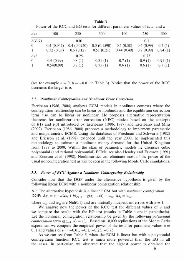
where � = 1 and c = 0. We will study the power of different noncointegration tests:the RCC, and the Engle–Granger (EG, 1987), for different parameter values ofthe parameter (b), say b = 0 (noncointegration), b = −0�01, −0�1, −0�25, −0�75(cointegration) and different short-run dependence given by a = 0� 1. This DGPfollows the parameterization used by Kremers et al. (1992) and Arranz andEscribano (2001). The results of EG are in parenthesis in Table 3.

Since the EG test is based on estimating the true error correction model (DGP),the EG test for noncointegration is more powerful than the RCC. However, theRCC is more powerful for small values of b, slow error correction EC adjustment


8


Table 3Power of the RCC and EG tests for different parameter values of b, a, and n

a\n 100 250 500 100 250 500

b�EG� −0�01 −0�10 0.4 (0.047) 0.4 (0.0920) 0.5 (0.1590) 0.5 (0.38) 0.6 (0.99) 0.7 (1)1 0.32 (0.09) 0.5 (0.12) 0.51 (0.21) 0.44 (0.49) 0.7 (0.99) 0.84 (1)

a\b −0�25 −0�750 0.6 (0.99) 0.8 (1) 0.81 (1) 0.7 (1) 0.9 (1) 0.91 (1)1 0.54(0.99) 0.7 (1) 0.75 (1) 0.6 (1) 0.6 (1) 0.7 (1)

(see for example a = 0, b = −0�01 in Table 3). Notice that the power of the RCCdecreases the larger is a.

3.2. Nonlinear Cointegration and Nonlinear Error Correction

Escribano (1986, 2004) analyzes ECM models in nonlinear contexts where thecointegration relationship can be linear or nonlinear and the equilibrium correctionterm also can be linear or nonlinear. He proposes alternative representationtheorems for nonlinear error correction (NEC) models based on the conceptsof I�1� and I�0� introduced by Escribano (1986, 1987) and Escribano and Mira(2002). Escribano (1986, 2004) proposes a methodology to implement parametricand nonparametric ECMS. Using the databases of Friedman and Schwartz (1982)and Ericsson et al. (1998), extended until the year 2000, he implemented thismethodology to estimate a nonlinear money demand for the United Kingdomfrom 1878 to 2000. Within the class of parametric models he discusses cubicpolynomial (and rational polynomial) ECMs; see also Hendry and Ericsson (1991)and Ericsson et al. (1998). Nonlinearities can eliminate most of the power of theusual noncointegration test as will be seen in the following Monte Carlo simulations.

3.3. Power of RCC Against a Nonlinear Cointegrating Relationship

Consider now that the DGP under the alternative hypothesis is given by thefollowing linear ECM with a nonlinear cointegration relationship.

H1: The alternative hypothesis is a linear ECM but with nonlinear cointegrationDGP: �yt = c + a�xt + b�yt−1 − g�xt−1� ��+ w1t, �xt = w2t,

where w1t and w2t are Nid(0,1) and are mutually independent errors with � = 1.We analyze now the power of the RCC test for different values of a and

we compare the results with the EG test (results in Table 4 are in parenthesis).Let the nonlinear cointegration relationship be given by the following polynomialcointegration term g�zt−1� �� = z

jt−1. Based on 10,000 replications of the Monte Carlo

experiment we compute the empirical power of the tests for parameter values a =0� 1 and values of b = −0�01, −0�1, −0�25, −0�75.

As we can see from Table 5, when the ECM is linear but with a polynomialcointegration function RCC test is much more powerful than the EG in allthe cases. In particular, we observed that the highest power is obtained for


9


Table 4Size adjusted power of the RCC test and the EG test (in parenthesis) at 5%

significance level based on H1 with g = zjt−1, j = 2� 3, and 4, for different sample

sizes n, different values of parameter b, and fixing the parameter a at a = 0

100 250 500 100 250 500

j\b −0�01 −0�25a = 0 2 0.71 (0.02) 0.86 (0.002) 0.94 (0.001) 0.88 (0.09) 0.98 (0.03) 1 (0.01)

3 0.88 (0.06) 1 (0.02) 1 (0.003) 0.9 (0.07) 1 (0.03) 1 (0.009)4 0.92 (0.04) 1 (0.01) 1 (0.001) 0.93 (0.08) 1 (0.03) 1 (0.01)

j\b −0�1 −0�75a = 0 2 0.88 (0.1) 0.96 (0.02) 1 (0.01) 0.9 (0.1) 0.95 (0.07) 0.98 (0.07)

3 0.94 (0.1) 1 (0.03) 1 (0.01) 0.9 (0.17) 1 (0.14) 1 (0.16)4 0.93 (0.1) 1(0.11) 1(0.10) 1(0.23) 1(0.234) 1(0.275)

j = 3 followed by j = 4 and j = 2, respectively. The intuition given by Escribano(2004) is the following: cubic polynomials are very flexible and can approximatedifferent level shifts. Furthermore, the error correction term in this case canbe equilibrium correcting (stable nonlinear adjustment) and therefore not adeviating error adjustment term as can happen with the quadratic polynomial.Notice that, as expected, the empirical power of the tests decreases with theparameter a even for large negative values of b. Let the nonlinear cointegratingfunction be g�zt−1� �� = exp�zt−1/100�. The size adjusted power of the RCCtest and the EG test (in parenthesis) for parameter values a = 0� 1 and b =−0�01�−0�05�−0�1�−0�25�−0�5�−0�75, are given in Table 6.

The power of the EG test is very low since this linear procedure misspecifiesthe estimation of the cointegrating vector by assuming that it is linear. When thereis no short-run dependence �a = 0� the power of the RCC is very high and it isreduced when the parameter a is large. This is due to the fact that if the short-rundependence is high, the nonlinearity also strongly affects the short-run dependenceof the cointegrating errors and therefore the power of those tests that do not takethis information into account is reduced. Similar results are obtained when the

Table 5Size adjusted power of the RCC test and EG test (in parenthesis) at 5%

significance level based on H1 with g = zjt−1� j = 2� 3, and 4, for different sample

sizes n, different values of parameter b and fixing the parameter a at a = 1

100 250 500 100 250 500

j\b −0�01 −0�25a = 1 2 0.35 (0.008) 0.5 (0.003) 0.65 (0) 0.45 (0.057) 0.6 (0.02) 0.7 (0.005)

3 0.6 (0.05) 0.7 (0.01) 0.87 (0.002) 0.6 (0.09) 0.8 (0.03) 0.9 (0.007)4 0.55 (0.04) 0.7 (0.01) 0.8 (0.002) 0.5 (0.09) 0.6 (0.02) 0.7 (0.005)

j\b −0�1 −0�75a = 1 2 0.5 (0.072) 0.6 (0.047) 0.8 (0.02) 0.3 (0.09) 0.4 (0.07) 0.6 (0.057)

3 0.6 (0.09) 0.8 (0.05) 0.9 (0.02) 0.45 (0.13) 0.64 (0.15) 0.8 (0.13)4 0.55 (0.09) 0.7 (0.13) 0.8 (0.09) 0.3 (0.24) 0.45 (0.23) 0.6 (0.27)


10


Table 6Size adjusted power of the RCC test and EG test (in parenthesis) at 5%

significance level based on H1 with g = exp�zt−1/100� for different sample sizes nand different values of parameters a and b

a = 0 a = 1

b\n 100 250 500 100 250 500

−0�01 0.4 (0.06) 0.48 (0.05) 0.5 (0.05) 0.4 (0.07) 0.45 (0.07) 0.46 (0.08)−0�05 0.43 (0.05) 0.52 (0.05) 0.57 (0.05) 0.43 (0.05) 0.46 (0.05) 0.5 (0.05)−0�1 0.5 (0.05) 0.61 (0.05) 0.7 (0.05) 0.43 (0.06) 0.5 (0.06) 0.6 (0.06)−0�25 0.6 (0.05) 0.8 (0.06) 0.82 (0.09) 0.5 (0.07) 0.54 (0.06) 0.7 (0.08)−0�5 0.65 (0.07) 0.85 (0.09) 0.9 (0.1) 0.52 (0.08) 0.57 (0.13) 0.76 (0.13)−0�75 0.7 (0.1) 0.9 (0.11) 1 (0.15) 0.6 (0.14) 0.65 (0.17) 0.8 (0.19)

nonlinear cointegrating function is g�zt−1� �� = log�zt−1 + 100�; see Garcia (2004).Polynomial transformations, cubic or rational, are flexible functional forms usedto study general nonlinear error correction adjustments in asymmetric contexts.Escribano (2004) justified those functional forms based on Pade’s approximations.In what follows we analyze the power of the noncointegration tests RCC and EGfor nonlinear error correction models.

H1: Linear cointegration with an NECDGP:

�yt = c + a�xt + f�yt−1 − �xt−1�+ w1t� (15)

�xt = w2t (16)

with w1t, w2t Nid(0,1) errors, mutually independent. Consider the following value ofthe linear cointegrating parameter � = 1, with different nonlinear adjustments, f�·�.Let the cointegrating error be Ut−1 = yt−1 − �xt−1 and let the NEC adjustment bethe following polynomial case:

f�Ut−1� = �Ut−1 − 0�2�U 2t−1� (17)

The functional form (17) is justified by the representation theorem of NECmodels of Escribano (2004) where the stability condition on the nonlinearadjustment is satisfied (−2 < df�Ut−1�

dxt−1< 0).

It is clear that the power of the RCC is much higher than the power of the EGand that the power of RCC decreases with the short-run dependence of both seriesmeasures by parameter a. Following Escribano (2004), we combine now both typesof linearities.

H1: Nonlinear cointegration in an NEC modelDGP:

�yt = c + a�xt + f�yt−1 − g�xt−1� ��+ w1t� (18)

�xt = w2t� (19)


11


Table 7Size adjusted power of the RCC test and the EG

test (in parenthesis) for different values ofparameter a small and n small of model (17)

a\n 100 250 500

0 0.7(0.04) 0.8 (0.03) 0.9 (0.02)0.5 0.6 (0.02) 0.7 (0.03) 0.8 (0.07)1 0.2 (0.08) 0.43 (0.02) 0.5 (0.01)

where w1t, w2t are Nid(0,1), mutually independent and where � = 1. We can considertwo types of nonlinearities in the cointegration relationship.

Let Ut−1 = yt−1 − log�xt−1� and substitute in (17). The size adjusted power of theRCC and EG tests are given in Table 7 if Ut−1 is included in (17). Similar powerresults are obtained for Ut−1 = log�yt−1�− �xt−1.

3.4. Linear Cointegration with Structural Changes in the Cointegrating Vector

There is a body of literature on the effects of cointegration testing in the presence ofstructural changes. In what follows we want to simulate different cases based on theDGP of Arranz and Escribano (2001) to evaluate the power of the RCC in this contextwhen the break point is in the middle of the sample. Table 8 shows that the RCC testis clearly more powerful than the EG test in the presence of structural breaks.

H1: Linear error correction and cointegration in the presence of structural changein the cointegrating vector

DGP:�xt = w1t� (20)

�yt = c + a�xt + b yt−1 − �c1D1t−1xt−1 + �xt−1��+ w2t� (21)

where w1t, w2t are Nid(0,1) errors, and mutually independent, where c1 measuresthe change in the cointegrating vector. We will consider the following values,� = 1, c1 = 2. The structural break is created by the artificial dummy variable D1t,defined by

D1t ={1� t ≥ n

2�

0 otherwise�(22)

Table 8Size adjusted power of the RCC test and theEG test (in parenthesis) for different values of

a and n when Ut−1 is included in (17)

a\n 100 250 500

0 0.72 (0.02) 0.85 (0.032) 0.93 (0.04)0.5 0.6 (0.02) 0.7 (0.04) 0.8 (0.02)1 0.35 (0.09) 0.42 (0.021) 0.45 (0.012)


12


Table 9Size adjusted power of the RCC test and EG test (in parenthesis) for different

values of parameters a, b, n and c1 = 2

c1 = 2a\n 100 250 500 100 250 500

b = −0�01 b = −0�025

0 0.5 (0.2) 0.65 (0.1) 0.66 (0.2) 0.65 (0.2) 0.8 (0.24) 0.85 (0.23)1 0.41 (0.05) 0.5 (0.03) 0.64 (0.02) 0.54 (0.01) 0.61 (0.01) 0.8 (0.007)

b = −0�5 b = −0�750 0.81 (0.23) 1 (0.25) 1 (0.25) 0.8 (0.25) 1 (0.26) 1 (0.29)1 0.62 (0.03) 0.8 (0.02) 0.9 (0.01) 0.61(0.06) 0.73(0.06) 0.91(0.07)

Based on 10,000 replications of the Monte Carlo simulations, we obtained thesize adjusted power of the tests RCC and EG, see Table 9.

Table 9 show that the RCC is more powerful than the EG test to reject thenull hypothesis of noncointegration in the presence of a structural break in thecointegrating vector. The power of the RCC is very good for moderate short-rundependence �a = 1� and when the parameter �b� of the error correction adjustmentis not slow. Those power results of the RCC test statistic are very promising;however, we need to find a small sample correction of the RCC test statistic tomake it invariant to the short-run dependence indicated by the parameter a. As wasmentioned in the previous section, the solution to this problem is in the test statisticthat we called RCCCD (RCC corrected for dependence). The idea of the correctionis to count the synchronicity of the jumps, or new records, of both series (y and x)but relative to the synchronicity of the jumps in the first differences of the series (�yand �x). The RCC with the correction for dependence is RCCCD mentioned before.We showed in Table 2 that the critical values of the RCCCD test statistic are nowindependent of the short-run correlation measured by the parameter a. The questionnow is to evaluate the impact of this small sample correction on the power of thetest. However, since the empirical distribution of the RCCCD is very similar to theRCC with a = 0, and since for a = 0 the RCC test was most powerful, we expect alsoto get important power improvements when a �= 0 by using RCCCD instead of RCC.

4. Empirical Applications

4.1. Analysis of Gold and Silver Prices

Gold and silver have been actively traded for thousands of years and remainimportant and closely observed markets. Here, following Escribano and Granger(1998), monthly prices are analyzed from the end of 1971 until 1996. We areinterested in testing the existence of contemporaneous relationships between theprices of the two commodities in log levels. These prices are determined in clearlyspeculative markets and therefore their behavior should be captured by unit-roottime series models. The unit root is supported by the Dickey Fuller (DF) type testsusing from 1 to 6 lags of the dependent variable and including constant and constantand trend variables in the regression equation. There is, however, a feature of this


13


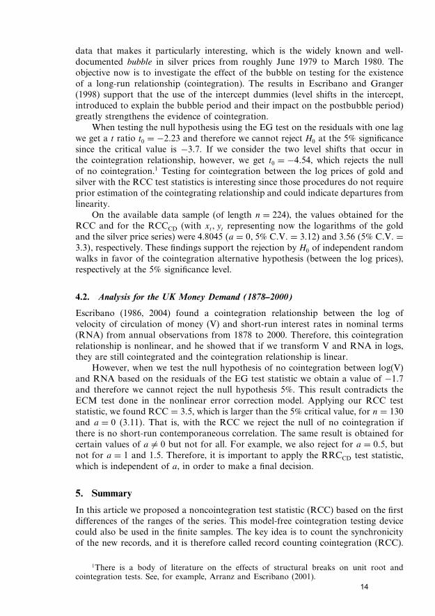
data that makes it particularly interesting, which is the widely known and well-documented bubble in silver prices from roughly June 1979 to March 1980. Theobjective now is to investigate the effect of the bubble on testing for the existenceof a long-run relationship (cointegration). The results in Escribano and Granger(1998) support that the use of the intercept dummies (level shifts in the intercept,introduced to explain the bubble period and their impact on the postbubble period)greatly strengthens the evidence of cointegration.

When testing the null hypothesis using the EG test on the residuals with one lagwe get a t ratio t0 = −2�23 and therefore we cannot reject H0 at the 5% significancesince the critical value is −3�7. If we consider the two level shifts that occur inthe cointegration relationship, however, we get t0 = −4�54, which rejects the nullof no cointegration.1 Testing for cointegration between the log prices of gold andsilver with the RCC test statistics is interesting since those procedures do not requireprior estimation of the cointegrating relationship and could indicate departures fromlinearity.

On the available data sample (of length n = 224), the values obtained for theRCC and for the RCCCD (with xt� yt representing now the logarithms of the goldand the silver price series) were 4.8045 �a = 0� 5% C�V� = 3�12� and 3.56 �5% C�V� =3�3�, respectively. These findings support the rejection by H0 of independent randomwalks in favor of the cointegration alternative hypothesis (between the log prices),respectively at the 5% significance level.

4.2. Analysis for the UK Money Demand (1878–2000)

Escribano (1986, 2004) found a cointegration relationship between the log ofvelocity of circulation of money (V) and short-run interest rates in nominal terms(RNA) from annual observations from 1878 to 2000. Therefore, this cointegrationrelationship is nonlinear, and he showed that if we transform V and RNA in logs,they are still cointegrated and the cointegration relationship is linear.

However, when we test the null hypothesis of no cointegration between log(V)and RNA based on the residuals of the EG test statistic we obtain a value of −1�7and therefore we cannot reject the null hypothesis 5%. This result contradicts theECM test done in the nonlinear error correction model. Applying our RCC teststatistic, we found RCC = 3�5, which is larger than the 5% critical value, for n = 130and a = 0 �3�11�. That is, with the RCC we reject the null of no cointegration ifthere is no short-run contemporaneous correlation. The same result is obtained forcertain values of a �= 0 but not for all. For example, we also reject for a = 0�5, butnot for a = 1 and 1�5. Therefore, it is important to apply the RRCCD test statistic,which is independent of a, in order to make a final decision.

5. Summary

In this article we proposed a noncointegration test statistic (RCC) based on the firstdifferences of the ranges of the series. This model-free cointegration testing devicecould also be used in the finite samples. The key idea is to count the synchronicityof the new records, and it is therefore called record counting cointegration (RCC).

1There is a body of literature on the effects of structural breaks on unit root andcointegration tests. See, for example, Arranz and Escribano (2001).


14


The series will not be cointegrated if there is a lack of synchronicity (up to aconstant delay) between the sequences of jumps or between the new records ofthe series. If the two series have a common stochastic component (common trend),their ranges will tend to jump together, indicating the synchronicity of the newrecords. The RCC test statistic clearly outperforms the traditional DF unit roottest on the cointegrating residuals (EG) as well as nonparametric tests in a similarcontext previously proposed by Aparicio et al. (2006a). The small sample propertiesof RCC nonparametric test are analyzed by Monte Carlo simulations and with someempirical examples. In particular, we test the null hypothesis of noncointegrationagainst the alternative hypothesis of a NEC or nonlinear cointegration or both.Furthermore, we are able to show that the RCC test for noncointegration is robustto nonlinearities and structural breaks. One important advantage of this RCCapproach is that it does not require previous estimation of the unknown (maybenonlinear) cointegrating relationship. Our Monte Carlo simulation analysis suggeststhat the proposed methodology is robust to different departures from the classicallinear cointegration context, like nonlinearities in the cointegrating relationship or inthe error correction term, or to structrual changes in the cointegrating relationship.The performance evaluation of the RCC in terms of size and power is comparedto the EG cointegration test. However, the RCC is sensitive to the short-rundependence between the series. Therefore, we suggest a small sample correction fordependence, the RCCCD, which works very well even in very small samples (goodsize and power properties). Finally, our RCC test statistic is applied to different datasets to show its usefulness in identifying cointegration in the presence of importantnonlinearities and structural changes.

Appendix

Lemma 1. Let xt =∑t

i=1 ei�1 where ei�1 are continuous i.i.d. random variables withbounded and symmetric pdf, zero means, and finite variances. Suppose that x0 also has abounded pdf and finite variance. And let J�n�

�x� = n−1/2∑nt=1 1��R

�x�t > 0�. Then we have

n∑t=1

1(�R

�x�t > 0

) = O�n−1/2�

Proof. See Aparicio et al. (2006a).

Proof of Theorem 1. Since xt is a random walk we have from Lemma 1,

n∑t=1

1��R�x�t > 0� = O�n−1/2� �⇒ P

(�R

�x�t > 0

) = O�t−1/2�

�⇒ [P(�R

�x�t > 0

)]2 = O�t−1�

�⇒n∑

t=1

[P(�R

�x�t > 0

)]2 = O�log n�

since from Euler’s formula we can write∑n

t=1 t−1 = log n+ �+ 1

2n + 112n2 +

O�n−4�� = 0�57721566 (Euler’s constant).Now if xt and yt are independent we have


15


E�RCC�n�x�y� =

n∑t=1

P(�R

�x�t > 0

)P(�R

�y�t > 0

)

=n∑

t=1

[P(�R

�x�t > 0

)]2 = O�log n��

Therefore, under H0, we can write for some positive constant �:

RCC�n�x�y = � log n+ �nV�

where V denotes a nondegenerate random variable with unit variance and �n definesthe asymptotic order for the standard deviation of RCC�n�

x�y. Our next objective is todetermine �n. To do this, first note that E�RCC�n�

x�y − � log n�2 = E��nV�2 = �2nE�V�

2

E� RCC�n�x�y�

2� = E

{ n∑t=1

n∑t′=1

1(�R

�x�t > 0

)1(�R

�y�t > 0

)1(�R

�x�t′ > 0

)1(�R

�y�t′ > 0

)}

=n∑

t=1

[P(�R

�x�t > 0

)]2 + 2n∑

t=1

n∑t′=t+1

[P(�R

�x�t �R

�x�t′ > 0

)]2

=n∑

t=1

[P(�R

�x�t > 0

)]2 +W�n�x�y �

where we let

W�n�x�y = 2

n∑t=1

n∑t′=t+1

[P(�R

�x�t �R

�x�t′ > 0

)]2

= 2n∑

t=1

n∑t′=t+1

P��R�x�t′ > 0 �R�x�

t > 0��2 P��R�x�t > 0��2

= 2n−1∑t=1

[P(�R

�x�t > 0

)]2 n∑t′=t+1

[P(�R

�x�t′−t > 0

)]2�

Now we observe that

n−1∑t=1

[P(�R

�x�t > 0

)]2 n∑t′=t+1

[P(�R

�x�t′−t > 0

)]2

= �2n−1∑t=1

t−1�log n− log t�

= �2�log n�2 − �2n−1∑t=1

t−1 log t

= �2�log n�2 − �2

{ n∑t=1

(t

n

)−1(log

t

n+ log n

)1n

}

= �2�log n�2 − �2�log n�2 − �2

{ n∑t=1

(t

n

)−1(log

t

n

)1n

}


16


� −�2∫ 1

1/n

log xx

dx

= 12�2�log n�2�

It follows:

Var�RCC�n�x�y� � � log n+ �2�log n�2 − E�RCC�n�

x�y��2

= � log n�

This entails that

�n = O��log n�1/2� and �log n�−1RCC�n�x�y → 1�

Acknowledgments

This research was partially supported by the project SEJ2005-05485, SEJ2005-06454, and European project HPRN-CT-2002-00232.

References

Aparicio, F. M. (1995). Nonlinear Modelling and Analysis Under Long-Range Dependencewith an Application to Positive Time Series. Ph.D. thesis, Swiss Federal Institute ofTechnology, Dpt. of Electrical Enginnering, Laussane (Suiza).

Aparicio, F. M., Granger, C. W. J. (1995). Nonlinear Cointegration and Some New Tests forComovements Modelling (Working Paper 95–15). Dept. of Economics of the Universityof California, San Diego.

Aparicio, F. M., Escribano, A., Garcia, A. (2004). A Range Unit Root Test. Working Paperof the Department of Statistics of Carlos III University.

Aparicio, F. M., Escribano, A., Garcia, A. (2006a). Range unit root (RUR) tests: Robustagainst nonlinearities, error distributions, structural breaks and outliers. Journal of TimeSeries Analysis 27:545–576.

Aparicio, F. M., Escribano, A., Garcia, A. (2006b). Synchronicity Between Financial TimeSeries: An Exploratory Analysis. Progress in Financial Markets Research. Nova Publishers

Arranz, M. A., Escribano, A. (2001). Cointegration testing under structural breaks: a robustextended error correction model. Oxford Bulletin of Economic and Statistics 62:23–52.

Dickey, A., Fuller, W. (1979). Distribution of the estimators for AR time series with a unitroot. Journal of the American Statistical Association 74:427–431.

Engle, R. F., Granger, C. W. J. (1987). Cointegration and error correction: Representation,estimation and testing. Econometrica 55:251–276.

Ericsson, N. R., Hendry, D. F., Prestwich, K. M. (1998). Friedman and Schwartz (1982)revisited: Assesing annual and phase average models of money demand in the UnitedKingdom. Empirical Economics 23:401–415.

Escribano, A. (1986). Cointegration, Time Co-trends and Error Correction Systems: AnAlternative Approach (C.O.R.E. Discussion Paper, 8715). University of Louvain.

Escribano, A. (1987). Error Correction Systems: Nonlinear Adjustments to Linear Long-runRelationships (C.O.R.E. Discussion Paper, 8730). University of Louvain.

Escribano, A. (2004). Nonlinear error correction: the case of money demand in the U.K.(1878–2000). Macroeconomic Dynamics 8:76–116.

Escribano, A., Granger, C. W. J. (1998). Investigating the relationship between gold andsilver prices. Journal of Forecasting 17:81–107.


17


Escribano, A., Mira, S. (2002). Nonlinear error correction models. Journal of Time SeriesAnalysis 23:509–522.

Franses, P. H., Haldrup, N. (1994). The effects of additive outliers on tests for unit rootsand cointegration. Journal of Business and Economic Statistics 12:471–478.

Friedman, M., Schwartz, A. (1982). Monetary Trends in the USA and the UK: Their Relationto Income, Prices, and Interest Rates, 1867–1975. Chicago: University of Chicago Press.

Garcia, A. (2004). Contrastes Basados en Recorridos para Raices Unitarias y Cointegracion.Ph.D. Dissertation. Universidad Carlos III de Madrid.

Granger, C. W. J. (1981). Some properties of time series data and their use in econometricmodel specification. Journal of Econometrics 16:121–130.

Granger, C. W. J. (1995). Modelling nonlinear relationships between extended memoryvariables. Econometrica 63(2):265–279.

Granger, C. W. J., Hallman, J. J. (1991). Long-memory series with attractors. Oxford Bulletinof Economics and Statistics 53:11–26.

Hendry, D. F., Ericsson, N. R. (1991). An econometric analysis of UK money demandin monetary trends in the USA and UK by Milton Friedman and Anna J. Schwartz.American Economic Review 81:8–38.

Johansen, S. Estimation and hypothesis testing of cointegration vectors in Gaussian vectorautorregresive models. Econometrica 59:1551–1580.

Kremers, J. J., Ericsson, N. R., Dolado, J. J. (1992). The power of cointegration tests.Economics and Statistics 54:325–348.

Leadbetter, M., Rootzén, H. (1988). Extremal theory for stochastic processes. Annals ofProbability 16:431–478.

Lindgren, G., Rootzén, H. (1988). Extremes values: theory and technical applications.Scandinavian Journal of Statistics 14:241–279.

Perron, P. (1990). Testing for a unit root in a time series with a changing mean. Journal ofBusiness and Economic Statistics 70:153–162.

Phillips, P. C. B., Perron, P. (1988). Testing for a unit root in time series regression.Biometrika 75:335–346.


18

Time Series Analysis Nonlinear Cointegration and Nonlinear Error Correction: Record Counting...

Documents

Transcript of Time Series Analysis Nonlinear Cointegration and Nonlinear Error Correction: Record Counting...