MAGIC COUNTING WITH INSIDE-OUT POLYTOPES A thesis ...

MAGIC COUNTING WITH INSIDE-OUT POLYTOPES

A thesis presented to the faculty of f i t San Francisco State University

In partial fulfilment ofZPI&MTV, N / 4

The Requirements for The Degree

Master of Arts In

Mathematics

by

Louis Ng

San Francisco, California

May 2018

Copyright by Louis Ng

2018

CERTIFICATION OF APPROVAL

I certify that I have read MAGIC COUNTING WITH INSIDE-OUT

POLYTOPES by Louis Ng and that in my opinion this work meets

the criteria for approving a thesis submitted in partial fulfillment of

the requirements for the degree: Master of Arts in Mathematics at San

Francisco State University.

Dr. Matthias Beck Professor of Mathematics

Dr. Joseph Gubeladze Professor of Mathematics

Dr. Serkan HostenProfessor of Mathematics

MAGIC COUNTING WITH INSIDE-OUT POLYTOPES

Louis Ng San Francisco State University

2018

In this paper, we investigate strong 4 x 4 pandiagonal magic squares (no entries re

peat; equal row sums, column sums, and diagonal sums, including the wrap-around

ones), strong 5 x 5 pandiagonal magic squares, weak 2 x n magic rectangles (repeat

ing entries allowed; equal row sums and equal column sums), and 2 x n magilatin

rectangles (no entries repeat in a row/column; equal row sums and equal column

sums). The magic counts depend on the magic sum or the upper bound of the

entries. We compute their counting quasipolynomials and the associated generating

functions by using a geometrical interpretation of the problems, considering them

as counting the lattice points in polytopes with removed hyperplanes.

I certify that the Abstract is a correct representation of the content of this thesis.

Chair, Thesis Committee Date

I thank Dr. Matthias Beck for all the support, guidance, and corrections

along the way. I also thank Dr. Joseph Gubeladze and Dr. Serkan Hosten

for being part of my thesis committee.

ACKNOWLEDGMENTS

v

TABLE OF CONTENTS

1 Introduction............................................................................................................ 1

2 Background............................................................................................................ 4

3 Methodology ......................................................................................................... 6

4 Strong 4 x 4 Pandiagonal Magic Squares.............................................................15

4.1 Structure ...................................................................................................... 15

4.2 Cubical C ount....................................................................................................19

4.3 Affine C ount.......................................................................................................30

5 Strong 5 x 5 Pandiagonal Magic Squares.............................................................33

5.1 Structure .......................................................................................................... 33

5 .2 Outline for the Cubical and Affine C ou n t....................................................36

6 Weak 2 x n Magic R ectangles................................................................................38

6 .1 Weak 2 x 2 n Magic Rectangles ....................................................................38

6.2 Weak 2 x (2n + 1 ) Magic R ectan gles .......................................................... 47

7 2 x n Magilatin Rectangles.................................................................. 50

8 Cliffhanger (a.k.a. Future Researches) ................................................................63

Bibliography ....................................................................................................................64

vi

LIST OF TABLES

Table Page

4.1 Number of strong 4 x 4 pandiagonal magic squares with strict upper

bound t .................................................................................................................30

4.2 Number of strong 4 x 4 pandiagonal magic squares with magic sum s. 32

6.1 Number of weak 2 x 2 magic rectangles with column sum s..40

6 .2 Number of weak 2 x 4 magic rectangles with column sum s ..40

6.3 Number of weak 2 x 6 magic rectangles with column sum s ..40

6.4 Number of weak 2 x 3 magic rectangles with even column sum s. . . 47

6.5 Number of weak 2 x 5 magic rectangles with even column sum s. . . 48

6 .6 Number of weak 2 x 7 magic rectangles with even column sum s. . . 48

7.1 Number of 2 x 2 magilatin rectangles with odd column sum s.52



7.4 Number of 2 x 2 magilatin rectangles with even column sum s ................53




vii

1

Chapter 1

Introduction

If someone is to ask how many 3 x 3 magic squares are there, one may say the answer

is eight, and they are

6 1 00

7 5 CO

2 9 400 1 6

CO 5 7

4 9 2

00 CO 4

1 5 9

6 7 2

4 CO 00

9 5 1

2 7 6

2 7 6

9 5 1

4 CO 00

4 9 2

3 5 7

00 1 6

6 7 to

1 5 9

00 CO 4

2 9 4

7 5 3

6 1 00

2

However, this answer made a few assumptions. First, we assumed squares that

are rotationally or reflectively images of each other are counted as different magic

squares. Also, we assumed that we are restricted to entries 1 , 2 , . . . , 9. What if we

are to use any integer from 0 to some integer t? What if we can use any positive

entries, except the magic sum is not 15 but some other number? We can also open

up the possibility of repeated entries.

Let a generic magic square be labeled in the style of a matrix. In this paper, we

will consider the eight magic squares in the example as distinct even though they

are all the same up to rotation and reflection. On the issue of repeated entries, we

will specify which one of three conditions — strong (al3 ^ a^y if (*, j ) ^

Latin (atJ ^ atj> if ( i ,j ) ^ ( * , / ) and al} ^ at>3 if ( i ,j ) / or weak (no

restrictions on repeated entries) — we will be using in each chapter. As for the range

of entries, only nonnegative entries are allowed, and we will provide two different

counts: cubical count (a^ < t for all i and j ) and affine count (magic sum equals

s) [7]. For example,

9 2 7

4 6 8

5 10 3

3

is counted when we do the cubical count with t > 1 1 , or when we do the affine count

with s = 18.

An n x n pandiagonal m agic square is defined as a square array where the

row sums akj f°r & € { 1 , 2 , • • •, n}) , the colum n sums (X^”=i aik for k G

{ 1 , 2 , . . . , n }), and the (w rap-around) diagonal sums (X^+j=fc (mod n) aij for k 6

{ 1 , 2 , . . . , n } and (mod» )aH for k e { 1 ,2 , . . . ,n}) are equal. A magilatin

rectangle has equal row sums and column sums while using the Latin condition.

Through the use of inside-out polytopes (details in Chapter 3) and other techniques,

this paper will focus on the cubical count and affine count of strong 4 x 4 pandi

agonal magic squares (Theorems 4.8 and 4.9 below), the structure of strong 5 x 5

pandiagonal magic squares (Theorem 5.3), the affine count of weak 2 x n magic

rectangles (Theorems 6 .1 , Corollary 6.7, and Thorem 6.9), and the affine count of

2 x n magilatin rectangles (Theorems 7.1, 7.2, 7.3, and 7.4).

4

Chapter 2

Background

When most people think of magic squares, they likely think of recreational mathe

matics. However, some people also use magic squares in art. In 2014, Macau issued

nine stamps of values one to nine pataca, printed on which are famous magic squares

and word squares [8 ]. For instance, on the four pataca stamp is the magic square

on German Renaissance artist Durer Albrecht’s engraving Melencolia I [1].

While fun and art are good reasons to study magic squares, they have practical

applications as well. In cryptography, magic squares can be used to encrypt images

[16, 18]. Statisticians use stochastic matrices (matrices of nonnegative entries with

row sum, column sum, or both row and column sums equal to 1), a specialized form

of magic squares [10].

5

Throughout the centuries, many studies have been done on the topic of magic

squares. In the early days of magic squ'are investigation, people mostly focused

on the construction of various magic squares. For example, De la Loubere in

troduced the Siamese method for generating (2 n + 1) x (2 n + 1 ) magic squares

[15]. Benjamin Franklin came up with an 8 x 8 magic square and a 16 x 16 magic

square with interesting properties [4]. Edouard Lucas, the mathematician famous

for the Lucas sequence, devised a generalization of all 3 x 3 magic squares. Some

other construction-related magic square problems include finding magic squares with

prime number entries [2 ] and finding magic squares with perfect square entries [13].

Though much research focuses on construction, mathematicians also enumerated

magic squares. If we use entries 1-16 (or 1-25 in the case of 5 x 5) and not count

magic squares that are the same up to reflection or rotation, there are 880 magic

squares of size 4 x 4 and 275,305, 224 magic squares of size 5 x 5 [11]. The count of

bigger magic squares is not known. As for cubical count and affine count, Matthias

Beck and Thomas Zaslavsky enumerated the number of magic, semimagic (diagonal

sums irrelevant), and magilatin 3 x 3 squares [7].

6

Chapter 3

Methodology

We will turn the problem of counting magic squares into a problem of combina

torial geometry. As such, we need to first define some geometry-related terms. A

hyperplane H^b is defined as

Ha,b {% = (x i ,x 2, . . . ,x d) e R d : a ■ x = b},

for some a = (ai, a2, . . . , a<j) 6 Rd \ (0 , 0 , . . . , 0 ) and 6 € R. A hyperplane splits Rd

into two open halfspaces

H~b {x = (x i ,x 2, ■■■ ,Xd) € R d : a - x > b} and

Hs,b :== = (x i>x 2 , ■ ■ ■ ,x d) e M d : a ■ x < b}.

7

Ha,b is the boundary of the open halfspaces H ?b and H~h. Taking the union of open

halfspaces and their boundaries, we get the closed halfspaces

H^i := {x — (x i ,x 2, . . . , Xd) e R d : a • x > b } and

H fh ■= {% = (x1,x 2, . . - , x d) E Rd : a- x < b } .

A convex* p o ly top e P is the bounded intersection of finitely many closed half

spaces. In other words,

n\ n2 TI3p = n ^ n n ^ n n ^ ,

2=1 2=1 2=1

The affine hull aff(P) of P is (^\{Hstb ■ P Q Hs,b}- The dim ension of a polytope

is the dimension of its affine hull. The relative interior o f a p o ly top e int(P) is

the interior of P relative to aff(P). The set int(P) has the representation

n\ ri2 713

m t ( P ) = n ^ n n ^ n n « 3 ^2=1 2=1 2=1

The dimension of the relative interior of a polytope is the same as the dimension of

the polytope. The relative boundary o f a p o ly top e is

dP — P \ int(P).

*A11 polytopes in this paper will be convex, so we will just call them polytopes

8

We can also represent a polytope as the convex hull of a finite set of points [5],

where the convex hull of p$, p%,. . . , pt, £ is

{h p t + &2j02 + * ' * + fcnPn '• kj > 0 and k\ + fv2 + • • • + kn = 1 } ,

The set of vertices of a polytope is the smallest set of points whose convex hull is

said polytope. The vertices of the relative interior of a polytope are the vertices of

the polytope. For more information on polytopes, [12] is a good resource.

With these definitions in mind, we return to magic squares. 3 x 3 magic squares

correspond to points (an, 012, . . . , 033) in E9. Note that the entries of a magic square

are all nonnegative integers, so the coordinates an, ai2, . . . , 033 € Z>0. Points with

integral coordinates are called lattice points. All we need to do now is to count

the lattice points (an, ai-2, ■ ■ ■, a33) that satisfy the conditions of the magic square

structure.

Under the cubical count, each entry is nonnegative and less than t, so one set of

conditions that we have are the inequalities 0 < atj < t for all i and j . Of course,

just bounding the entries does not make the square magic, so we need to equate the

sums of each line (entries that we sum such as ones in a row). In the case of a 3 x 3

magic square, the equations are a n + a i2+ a i3 = a2i+ a 22+ a 23 = • • • = ai3+ a 22 + a3i.

Finally, we need to forbid duplicate entries. We can do so by setting nonequalities

9

pairwise between coordinates (like an ^ ai2).

For the affine count, one set of equations is to set each line sum to s, i.e., an + a\ 2 +

ai3 = s, a2i + 0,22 + «23 = s, etc. We also need the set of inequalities atJ > 0 for

all i and j . Lastly, just as the cubical count, we need nonequalities to take care of

duplicate entries.

With the strong condition, the magic square can only have at most one 0. If we

designate an a^j* to be 0 , then the inequalities atJ > 0 become strict inequalities

a,ij > 0 for all ( i ,j ) ^ (i* ,j*). We will discuss the logistics of designating a 0 later

in the paper.

In general, not just for 3 x 3 magic squares, without applying the nonequalities

for duplicate entries, the equations and strict inequalities will result in the relative

interior of a rational polytope (vertices have rational coordinates). Let the polytope

be Pf for the cubical count and P “ for the affine count. Equations such as an — an

are hyperplanes. Let TL be the set of hyperplanes that accounts for the duplicate

entries. Forcing an ^ ai2 is the same as removing a hyperplane from the relative

interior of a rational polytope. Therefore, we need to find |(int(Ptc) \ (J %) H Zd\ and

|(int(Psa)\ U ^ )n Z d|. The pairs (Ptc,%) and (P “ ,H ) are inside-out polytopes [5].

10

As we change the value of the maximum entry limit t, the set int(Ptc) \(J H changes.

The equations for the line sums and the noninequalities for duplicate entries do not

change, but the inequalities 0 < atj < t do. All of these restrictions dilate about

the origin with t. In other words,

int(Ptc) \ (J H = t (int(P°) \ |J U) = [tx e R : x £ int{P‘ ) \ (J •

This is similarly true when we increase the magic sum 5 as we do the affine count.

For simplicity, we will forgo the subscript 1 , i.e., P° = Pf and P a = P “ .

The notation for the number of lattice points in a set S dilated by n is L(S, n) —

InS fl Z d|. The associated generating function is the Ehrhart series

Ehr5 (a:) = 1 + J ] L(5, n )sn.n> 1

For int(5 ), the interior of a polytope, the Ehrhart series is

Ehrint(5 ) (x) = ^ L (in t(5 ') ,n )a ;n.n> 1

In general, the generation function of a sequence an is J2n>oanxn-

Proven by Eugene Ehrhart (the namesake of the Ehrhart series), the number of

lattice points in a dilated rational polytope nP follow a quasipolynomial

L(P, n) = cdimp(n)ndimP H h ci(n)n + co(ra),

where c0, c i , , CdimP are periodic functions, the period of each c3 divides the least

common denominator of the coordinates of all vertices, and Cdimp(n) is nonzero for

some n [9]. As a quasipolynomial with n as a variable, L(P , n) can be evaluated at

n < 0 . The function L(int(P),n) is also a quasipolynomial, and Ian G. Macdonald

showed that [17]

L (P ,-n ) = (—l )dimPL(int(P),n).

As for their Ehrhart series,

Ehrint(p) (x) = (—l ) 1+dimPEhrp Q ) . (3 .1)

Unfortunately, int(nP) \ (J Ti is not a dilated polytope. However,

12

n i n-2 713

— 71 n h a * n n n n ^ n u « i u u ■ ■ •u Hki—1 i= l i= l/ ni n2 ri3

u n n h a * n n n n n ( * & » , u u • • •u ^i= l z=l i= 1

Til 712 7i3U » f l f fa * n f | Hi A n f| n ( f f | Al u h %m u ■ • • u ^ )

V.i=l i= l i= 1

is the union of finitely many disjoint relative interiors of dilated rational polytopes.

Let us call each of these disjoint relative interiors of rational polytopes a region (if

it is nonempty). The closure of each region is some polytope R. The observation

above gives us

L (int(P) \ [ j U, n ) = L(int(R), n),

summing over all regions. As for its Ehrhart series,

Ehrint(p)Mj W(a;) := £ L ( i n t ( P ) \ U ^ , n ) xnn> 1

= '^ 2 '^ 2L (m t(R ),n )xnn> 1 R

= 5 Z L(int(R )in)xnR n> 1

= ^ E h r int(ji)(i).R

13

Counting the lattice points in each region is challenging; the dimension of each

region is dim(P). If we apply (3.1) to each region int(R) and plug in j , we obtain

£ E h r M(fl) ( } ) = (—l ) 1+dimP^ ^ Ehrjj(x).R R

Note that all regions have the same dimension as P, so factoring out (—l ) 1+dimP

is justified. ^ Ehr^(i') counts the lattice points in each region along with their

boundaries. Since the regions have overlapping boundaries, some lattice points are

counted more than once. For example, lattice points on a hyperplane Hgjb in H in

int(P) are counted at least twice: once for boundaries of regions in the halfspace

b and once for boundaries of regions in the halfspace H~h. Lattice points on the

intersection of two hyperplanes in the relative interior of the polytope are counted

four times (the lattice points are on the boundaries of regions in the > or < side of

the two hyperplanes). Taking all the extra counts in consideration, we have

X^EhrR{x) = A(S )EhrniesHinp(x )R S'C[n]

where T-L = {Hi : 1 < i < n}, [n] = {x € Z : 1 < x < n}, and A(S) is a coefficient

to account for the number of times an intersection Hies HiC\ P should be counted.

All but one term of the sum count the lattice points of a polytope of dimension less

than dim(P).

14

By the inclusion-exclusion principle, Matthias Beck and Thomas Zaslavsky demon

strated that [6 ]

^ E h r int(ii)(x) = ^2fi(u )E hiu(x).R uec

To unpack this equation, let us start with the partially ordered set C. As sets,

C = {fli€Sc[n] Hi H in t(P )}1'. The order -< is defined by reverse inclusion, i.e., for

any A, B €. C, A -< B if and only if B C A.

The function / / : £ —> Z is the M obius function

V{A) :=1 if int(P) = A,

— n(B) if int(P) -< A.BX.4

Applying 3 .1 to each Ehru(x) and Putting everything together, we get

-E h rint(P)MJW ( i J = ^ |/i(«)|Ehra(a:),uEjC

where u is the topological closure of u.

tint( P ) £ £ because int(P) = f ] ;e 0 H i ^ int(P).

15

Chapter 4

Strong 4 x 4 Pandiagonal Magic Squares

4.1 Structure

If we are to directly apply the counting method outlined in Chapter 2 to compute

the number of 4 x 4 magic squares, the most obvious difficulty stems from the

number of entries that 4 x 4 magic squares have; we would need a 16-dimensional

polytope! This is a rather daunting task. Instead, we will make use of the structure

and symmetries of 4 x 4 magic squares to make the calculation much simpler.

Lem ma 4.1. In a 4 x 4 pandiagonal magic sguare, the diagonal skip-over sums

satisfy an 4- <233 = <213 + <231, &i2 + (J34 = ax4 -I- 032, 021 + 043 = <123 + an , and

& 22 + 0,44 — a24 + a42 ■

Proof. In a 4 x 4 pandiagonal magic square, au + 0 2 2 + 33 + 44 = « i3 + « 22+ a 3i + « 44-

Subtracting a22 + 044 and we get an + 033 = 013 + 031. The other equations can be

16

proved the same way. □

Lem m a 4.2. In a 4 x 4 pandiagonal magic sguare with magic sum s, all diagonal

skip-over sums equal |.

Proof. Let an + a33 = ai3 + 0,31 = a and 012 + a34 = 014 + a32 = 6 (valid by Lemma

4.1). Consequently,

2 s = an + a33 + aj3 + a31 + ai2 + a34 + ai4 + a32

— 2 a -j- 26,

so s = a + b. Similarly, if a2i + a43 = a23 + 041 = c, then s = a + c. Therefore, b = c.

Next, consider the diagonal on entries au, a23, a32, 041-

s = ai4 + a23 + a32 + 041

= b + c

- 2b.

Thus, all diagonal skip-over sums are |. □

Lem m a 4.3. In a Ax A pandiagonal magic square with magic sum s, all 2 x 2 arrays

of adjacent entries also have sum s.

Proof. Due to symmetry, it is enough to show that the center entries sum to s. The

sum of the middle two columns and the middle two rows is 4s. Taking away the

17

wrap-around diagonals on the entries o13, a24, o3i, o42 and 012, 021, 034, 043, we get

twice the sum of the center entries equaling 2s. □

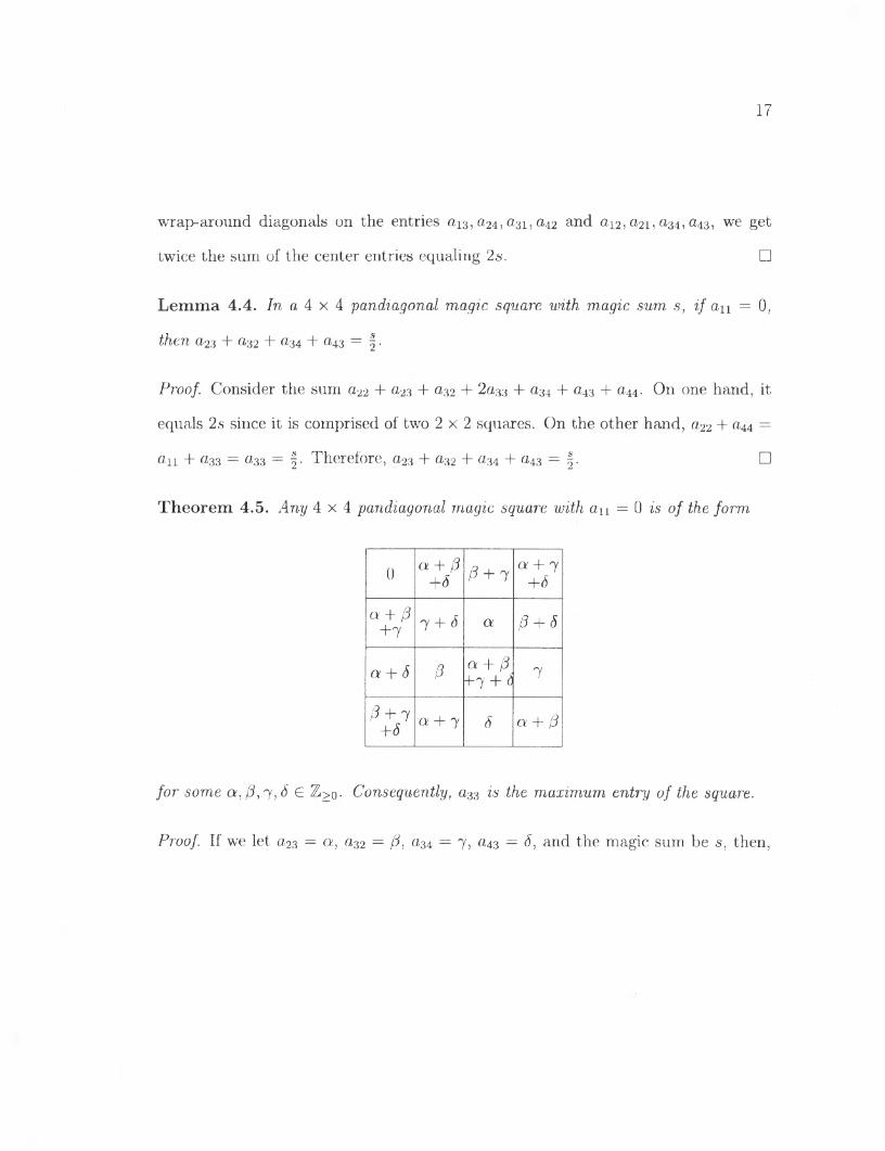
Lem m a 4.4. In a A x A pandiagonal magic square with magic sum s, if an = 0,

then 023 + 032 + 034 + 043 = § •

Proof. Consider the sum a22 + o23 + o32 + 2 a33 4- a34 -f a43 + a44. On one hand, it

equals 2 s since it is comprised of two 2 x 2 squares. On the other hand, a22 + o44 =

011 + 033 = 033 = |. Therefore, 023 + 032 4- 034 + a43 = |. □

Theorem 4.5. Any 4 x 4 pandiagonal magic square with an = 0 is of the form

0a + (3 +6 0 + 7

ot + 7 +6

a + (3 + 7 7 + 6 a (3 + 5

a + 6 Pa + (3 + 7 + <5 7

P + l +6 a + 7 6 Q! 4* (3

for some at, (3, 1,6 6 Z>o- Consequently, 033 is the maximum entry of the square.

Proof. If we let 023 = a, o32 = (3, a34 = 7 , a43 = 6, and the magic sum be s, then,

18

by Lemmas 4.2 and 4.4,

a + P + 7 + 5 = ^

— °11 + a 33

= a33

We can then use Lemma 3 and row sums to fill out the rest of the square. □

With Theorem 4.5, we reduced the number of variables to four.

As a side note, we can use this structure to construct interesting pandiagonal magic

squares. For example, here is one for any computer scientist or robot reading this

paper: __________________________

0 1101 1010 111

1011 110 1 1100

101 1000 1111 10

1110 11 100 1001

19

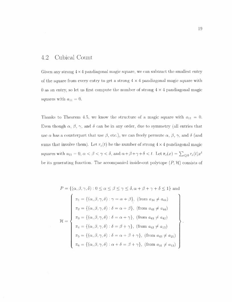
4.2 Cubical Count

Given any strong 4 x 4 pandiagonal magic square, we can subtract the smallest entry

of the square from every entry to get a strong 4 x 4 pandiagonal magic square with

0 as an entry, so let us first compute the number of strong 4 x 4 pandiagonal magic

squares with an = 0 .

Thanks to Theorem 4.5, we know the structure of a magic square with an = 0.

Even though a, f3, 7 , and 5 can be in any order, due to symmetry (all entries that

use a has a counterpart that use /3, etc.), we can freely permute a, (3, 7 , and 8 (and

sums that involve them). Let rc(t) be the number of strong 4 x 4 pandiagonal magic

squares with an = 0, a < f3 < 7 < 5, and a+(3+'y + 8 < t. Let rc(ar) = ^ <>0 rjfyx*

be its generating function. The accompanied inside-out polytope (P, T-L) consists of

P = {(a,/3,7 , 5 ) : 0 < o ; < / 3 < 7 < < 5 ,a + /3 + /y + 8 < l } and

7T! = {(a , /3,7 , (5) : 7 = a + fi}, (from a34 ± a44)

7T2 = {(a , (3,7 , J) : 5 = a + /?}, (from a43 ^ a44)

7T3 = {(a , /3,7 , 8) : 8 = a + 7 }, (from a43 ^ a42)

7r4 = {(a , p, 7 , 8) : 8 = /? + 7 }, (from a43 7 ai3)

7t5 = {(a , /3,7 , <5) : 8 = a + 0 + 7 }, (from a43 7 a2i)

7r6 = {(a , fi, 7 , <5) : a + 8 = ft + 7 }, (from a31 7 aj3)

ft = < > .

20

The vertices of P are

O = (0, 0, 0, 0), A = (0, 0, 0, 1), B = (o, 0, J ) , C = ( 0 , | , § , § ) , D = (I , I, I, I ) .

Now we need to find the intersections of elements of H in P and their Mobius

function values. If we label the following points

E = (0, i , 1 ,1 ) £ AC, F = (i, 1,1,1) e AD, F' = (1 ,1 , i,i)€AD,

G = (1,|, 1,1) S B C = (1,1, |, |) 6 A B A H' = (\ ,\ ,\ ,\ )£A B D ,

r _ / l l i 3\ c AC111 1 — (1- I A 2 \1 — V 8 ’ 4 ’ 4 ’ 8 / c ^ ° V 10’ 5 ’ 10’ 5 / ’

then the intersections are:

Zero hyperplanes:

0 : OABCD

One hyper plane:

tti: OACG

7r2: OCFG

tt3: OBCF

7T4: OBEF

7t5: OBEF'

tt6: O B D E

21

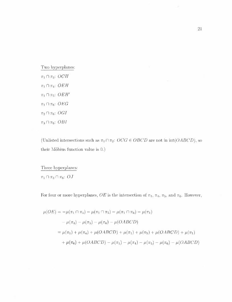
Two hyperplanes:

7Ti n 7r3: OCH

7Ti n7r4: OEH

7Ti D 7T5: OEH'

7Ti n 7T6: OEG

7t2 n 7t6: O G /

7r3 n 7r6: O B /

(Unlisted intersections such as 7Ti n 7 : OCG £ OBCD are not in int(0^4BCZ)), so

their Mobius function value is 0 .)

Three hyperplanes:

7Ti n 7T3 n 7T6: 0 ,7

For four or more hyperplanes, OE is the intersection of iti, n4, 7r5, and 7r6. However,

n(OE) = -U fa n 7r4) - ti(m n 7r5) - /x(7rx n 7r6) - ufa)

- /i(7T4) - /i(7r5) - //(7T6) - fi(OABCD)

— IjL( 7Ti) + /i(7T4) + /l(OABCD) + /i(7Ti) + //(tTs) + fJ,(OABC D) + /i(7Ti)

+ + n(OABCD) - £t(7Ti) — /x(7T4) - /i(7Tg) — /i(7T6) — fJ,(OABCD)

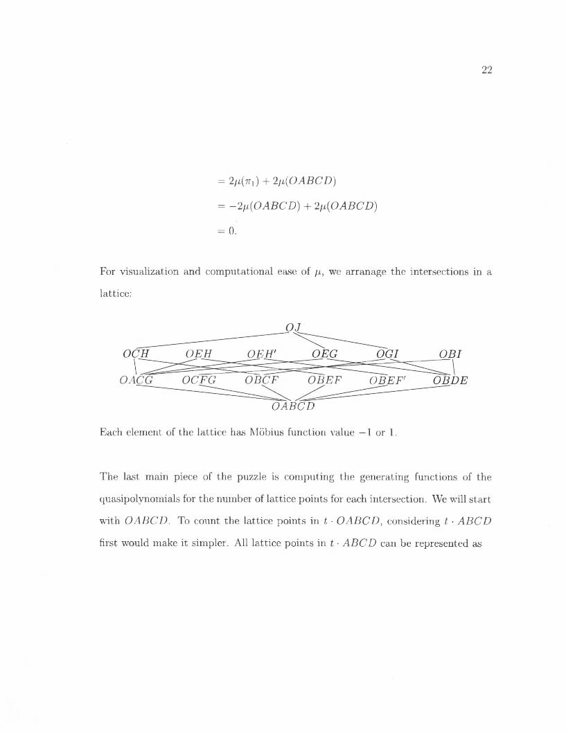
22

- 2/i(7Ta) + 2n(O AB C D )

= - 2 n{O ABCD ) + 2 n(O ABCD )

= 0 .

For visualization and computational ease of /i, we arranage the intersections in a

lattice:

OEH1

OACG O CFG O B C F O B E F OBEF'

O ABCD

OEH

Each element of the lattice has Mobius function value — 1 or 1 .

The last main piece of the puzzle is computing the generating functions of the

quasipolynomials for the number of lattice points for each intersection. We will start

with OABCD. To count the lattice points in t • OABCD, considering t • AB C D

first would make it simpler. All lattice points in t ■ A B C D can be represented as

23

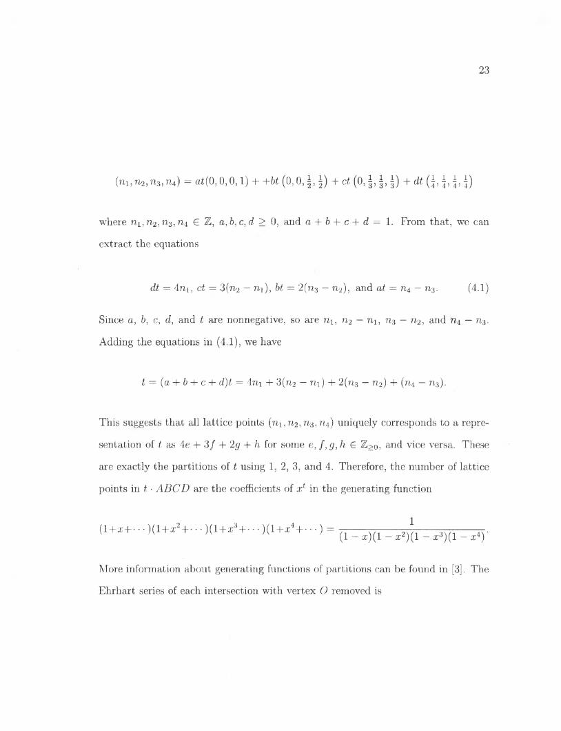
(n i,n2,n 3,n4) = a t(0 ,0 ,0 ,l) + + b t (0 , 0 , |) + ct (0 , |) + dt Q , J, j , J)

where n i, n2, n3, n4 € Z, a, b,c,d > 0 , and a + b + c + d = 1 . From that, we can

extract the equations

dt — 4ni, ct — 3(n2 — ni), bt — 2(n3 — n2), and at = n4 — n3. (4.1)

Since a, b, c, d, and t are nonnegative, so are n\, n2 — n\, n3 — n2, and — n3.

Adding the equations in (4.1), we have

t — (a + b + c + d)t = 4ni -I- 3(n2 — ni) + 2(n3 — n2) + (n4 — n3).

This suggests that all lattice points (ni, n2, n3, n4) uniquely corresponds to a repre

sentation of t, as 4e + 3 / + 2g + h for some e, f ,g ,h € Z>0, and vice versa. These

are exactly the partitions of t using 1 , 2 , 3, and 4. Therefore, the number of lattice

points in t, ■ A B C D are the coefficients of x l in the generating function

(1+xH------) ( l + x 2-\-----)(l+ :r3H-------) (1 + x 4H------) =(1 — x )(l — x2)(l — x3)( l — x4) '

More information about generating functions of partitions can be found in [3]. The

Ehrhart series of each intersection with vertex O removed is

24

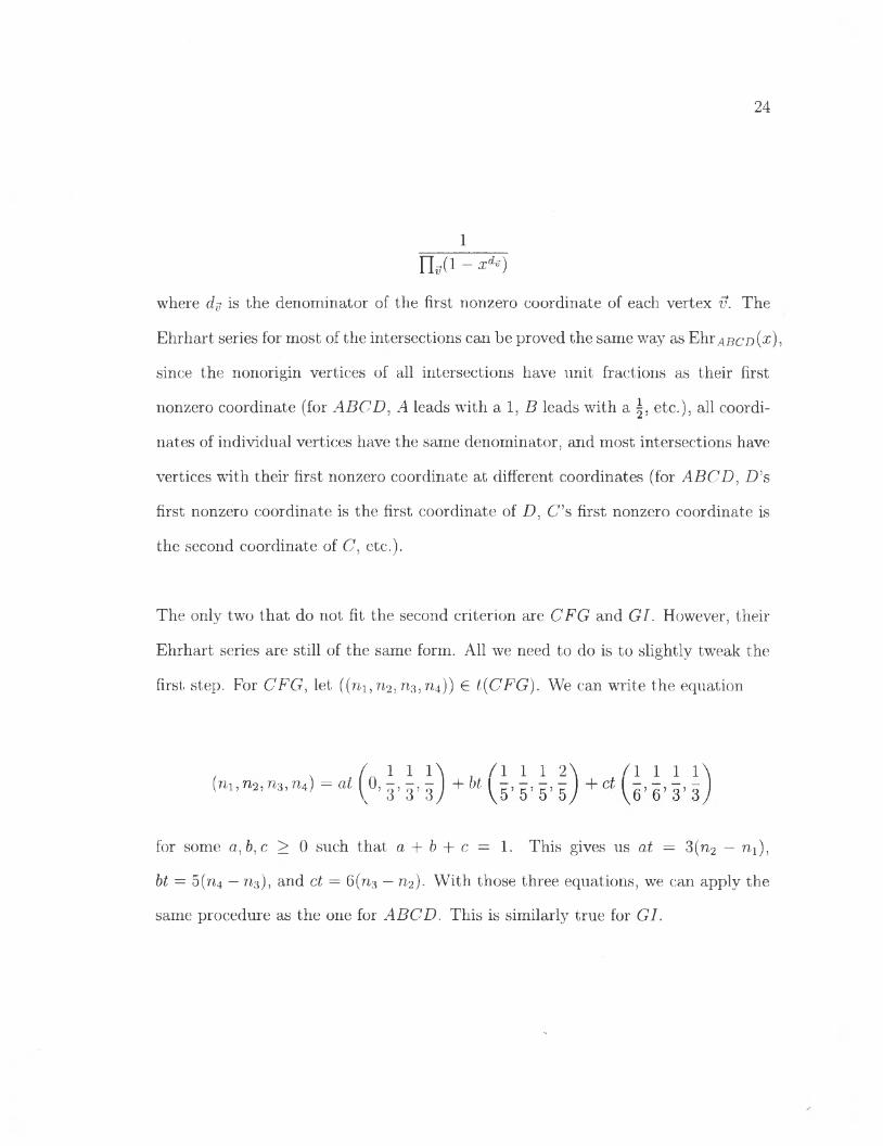
ryi - xd*)where dg is the denominator of the first nonzero coordinate of each vertex v. The

Ehrhart series for most of the intersections can be proved the same way as Ehr^pcD^),

since the nonorigin vertices of all intersections have unit fractions as their first

nonzero coordinate (for A B C D , A leads with a 1 , B leads with a etc.), all coordi

nates of individual vertices have the same denominator, and most intersections have

vertices with their first nonzero coordinate at different coordinates (for A B C D , D ’s

first nonzero coordinate is the first coordinate of D, C ’s first nonzero coordinate is

the second coordinate of C, etc.).

The only two that do not fit the second criterion are C FG and GI. However, their

Ehrhart series are still of the same form. All we need to do is to slightly tweak the

first step. For C F G , let ((ni, n2, n3 , 714)) € t{CFG ). We can write the equation

1

/ 1 1 1 \ , / I 1 1 2 \ / l 1 1 1 \( » . , » 3, nt ) = o( ( 0 , j , j , j ) + bt - j

for some a, b, c > 0 such that a + b + c — 1 . This gives us at = 3(n2 — ni),

bt — 5 (n4 — ro3), and ct = 6 (n3 — n2). With those three equations, we can apply the

same procedure as the one for ABCD . This is similarly true for GI.

25

To go from Ehrhart series such as Ehr abcd(x ) to Ehroabcd(%), we will use the

following claims:

Lem m a 4.6. Suppose the rational hyperplane Hgij £ Rd satisfies the following con

ditions:

• M• Hgj, contains a lattice point,

• the distance between Hgj, and O is less than or equal to the distance between

H^b and any lattice point not on &.*

Then Z rf C \JkeZ kHs,b-

Proof. Let Hgj, be a hyperplane that satisfies the conditions in the lemma. Let p be

a lattice point in H$b- The distance between H and p is 0, so a ■ p == b. Let lattice

point q £ H^b- The distance between H^b and q is for some ki € R.

q — np is also a lattice point for any n £ Z, and the distance between H and q — np

is Since tJMt, the distance between H and O, is less than or equal toINI IMP ’ M INI

for all n € Z, ki must be an integer. This tells us a ■ q — kb for some k £ Z. By

definition, q € kH^b- □

*The distance between the hyperplane H j j , and the point p is "^ -j^ .

26

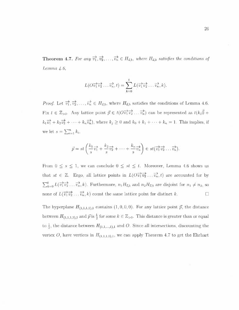
T heorem 4.7. For any v$, , ■ ■ ■, Vn € Hs,b, where Hs,b satisfies the conditions of

Lemma 4-6,

t

L(Oviv2 • . . «£,*) = L (vtv2 . . .v t ,k ) .k= 0

Proof. Let ui , V2 > ■ • • > ^ € Hs,b, where t satisfies the conditions of Lemma 4.6.

Fix t € Z >0. Any lattice point p € t(O vtv 2 ■ ■ ■ Vn) can be represented as t(kQ0 +

kivt + k2V2 + -----1- knv*), where kj > 0 and k0 + ki H h kn = 1 . This implies, if

we let s = Y h=i h ,

—* , f k\—y k‘2—y k7l— ^p = st \ — Vi H v2 + -------1 vn e stlvi v2 . . . vn).

\ s s s )

From 0 < s < 1 , we can conclude 0 < st < t. Moreover, Lemma 4.6 shows us

that st 6 Z. Ergo, all lattice points in L ( O v t . . . v^,t) are accounted for by

Ylk=o L(v\V2 ■ ■ - Vn, k). Furthermore, riiH^b and n2Hstb are disjoint for n\ ^ n2, so

none of L(v\v2 . . . v i, k) count the same lattice point for distinct k. □

The hyperplane contains (1 ,0 ,0 , 0 ). For any lattice point p, the distance

between and p is | for some k € Z>0. This distance is greater than or equal

to |, the distance between and O. Since all intersections, discounting the

vertex O, have vertices in H(l.i.i.i),!, we can apply Theorem 4.7 to get the Ehrhart

27

series

Ehr0£+j+ £+(x) = 1 + L(Ov\ v2 ■. ■ vn,t)x tt> 1

t= 1 + ^ 2 ^ 2 L (vlv2 ■■■vti, k)xl

t>l fc=0

= X1 + L(v1 V2 - - - vti, 1)^ X1 + •' •i> 0 i> 0

= xi 11+ l(vtv2 ...vt, t)x* Ji> 0 \ t>0 /

Y^T^Ehrvtv2...y (:Z')

_ 1___________

(! -*) n 1 - **ofor each intersection where d$ is the denominator of the first nonzero coordinate of

each non-origin vertex vJ. We now have the ingredients for rc(x).

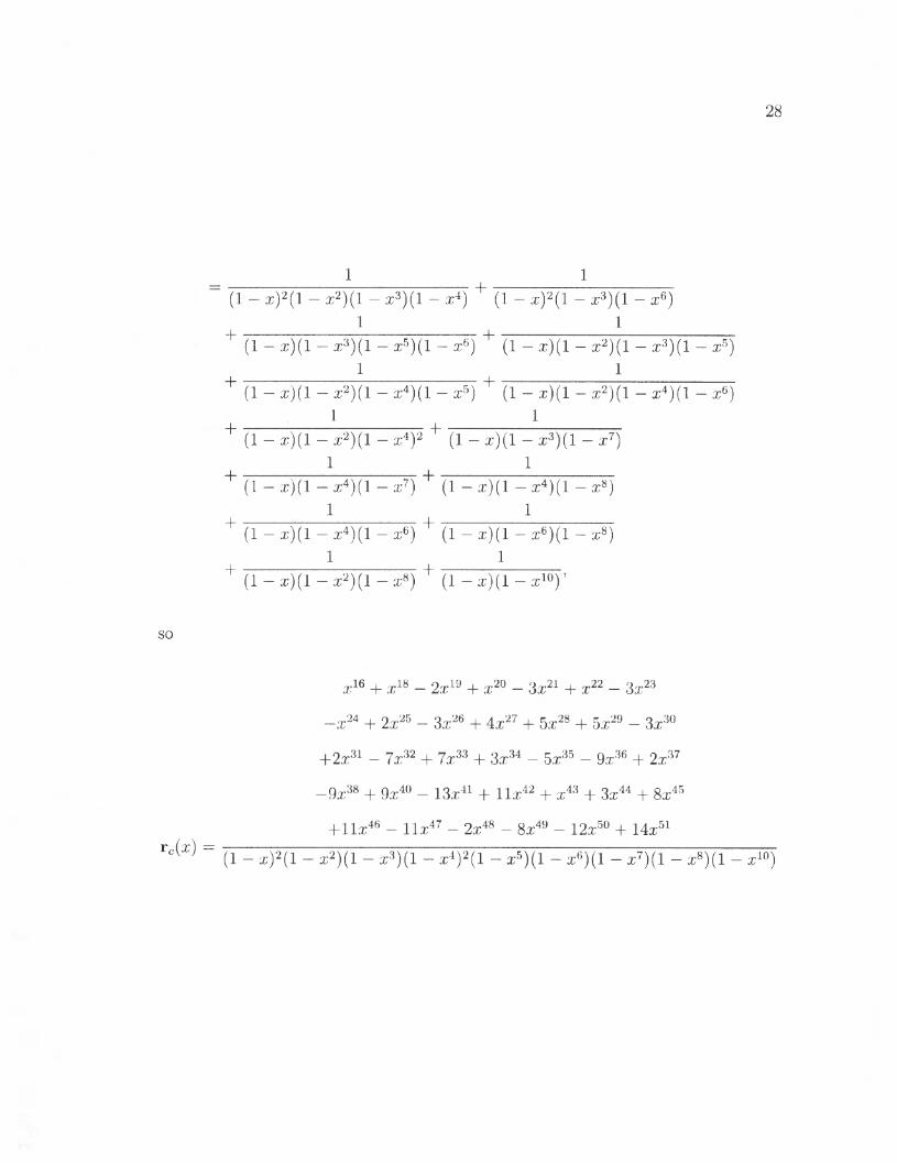
—rc y ~ j = EhrcMBoo^) + Ehr0y4CG(x) + Ehrocfg(x ) + Ehr0BCF(x)

+ EhrOB£;^(a;) + Ehr0 BKF'(^) + ^^o b d e (x ) + Ehr0 cj^(^)

+ EhraEtf(:r) + Ehr0 £H'(.x) + Ehr0 £;G(x)

+ EhroG/(x) + Ehr0 jB/(a:) + Ehr0 j(o:)

TFrom the first line to the second line, 1 = L ( v l v 2 . . . v%, 0) since O is the one and only point in 0 • V 1 V2 ■ ■ ■ v ti-

28

so

1+

1

+

+

1 — x)

(1 — x)2(l — x2)(l — x3)(l — a;4) (1 — x)2(l — x3)(l — a:6)1 1

+

1 — x)

1 — x)

1 — x)

1 — x)

1 — x)

1 — x3)(l — x5)(l — a;6) (1 — x)(l — x2)(l — x3)(l — x5)1 1

+1 — x2)(l — x4)(l — a;5) (1 — x)(l — x2)(l — x4)(l — a:6)1 1

+1 — x2)(l — a:4)2 (1 — x)(l — x3)(l — x7)1 1

1 — x4)(l — x7) (1 — x)(l — x4)(l — a:8)1 1

+1 — x4)(l — x6) (1 — x)(l — x6)(l — a;8)1 1

+1 — re2) (1 — a;8) (1 — x)(l — a;10) ’

rc(z) =

x + x 18 — 2x19 + a:20 — 3 a;21 + x “

—x 24 + 2a;25 — 3a;26 + 4a;27 + 5a;28 + 5a:29 — 3a:30

+2x31 — 7x32 + 7x33 + 3a;34 — 5a;35 — 9x36 + 2a:37

—9a;38 + 9a;40 — 13a:41 + 11a;42 + x43 + 3a;44 + 8 a;45

+ l l x 46 - 11a;47 - 2a;48 - 8a;49 - 12a;50 + 14x51

(1 — x)2(l — x2)( l — x3) ( l — x4)2(l — x5)( l — x6)( l — x7)( l — x8) ( l — x10)

.22 3x23

29

x16(l — a;2)

/ 1 + 2x + 6 a;2 -I- 8a;3 + 17a;4 + 20a;5 + 36a:6

+38x7 + 58a;8 + 57a;9 + 76a;10 + 6 8 a;11 + 84a:12 + 70x13

+81a;14 + 57a;15 + 59a;16 + 34a;17 + 38a;18 + 16a;19 + 14a;20

(1 — a;3)( l — a;4)( l — a:6) ( l — a;7)( l — a;8)( l — a;10)

Recall that rc(x) enumerates strong 4 x 4 pandiagonal magic squares with a < <

7 < 5 , an = 0, and a33 < t. For a strong 4 x 4 pandiagonal magic square with

nonnegative entries, there are three things to tweak:

(1 ): the smallest entry does not have to be 0 ,

(2 ): the smallest entry could have been any one of the sixteen atj , and

(3): a, /3, 7 , and 8 could be ordered in one of 24 permutations.

Fixes (2 ) and (3) are easy to make; we only need to multiply the count by 384. Let

us reason through fix ( 1 ). To make the smallest entry nonzero, we can add one to

every aij. We could also have added two to every a^. Any integer added to all

aij would result in a new magic square. Adding one pushes the maximum entry by

one, so we multiply the generating function by x\ Adding two pushes the maximum

entry by two, so we multiply the generating function by a;2; so on and so forth. This

means we need to multiply rc(a;) by 1 + x + x 2 4 - • • • = y ~ - This gives us the final

30

count.

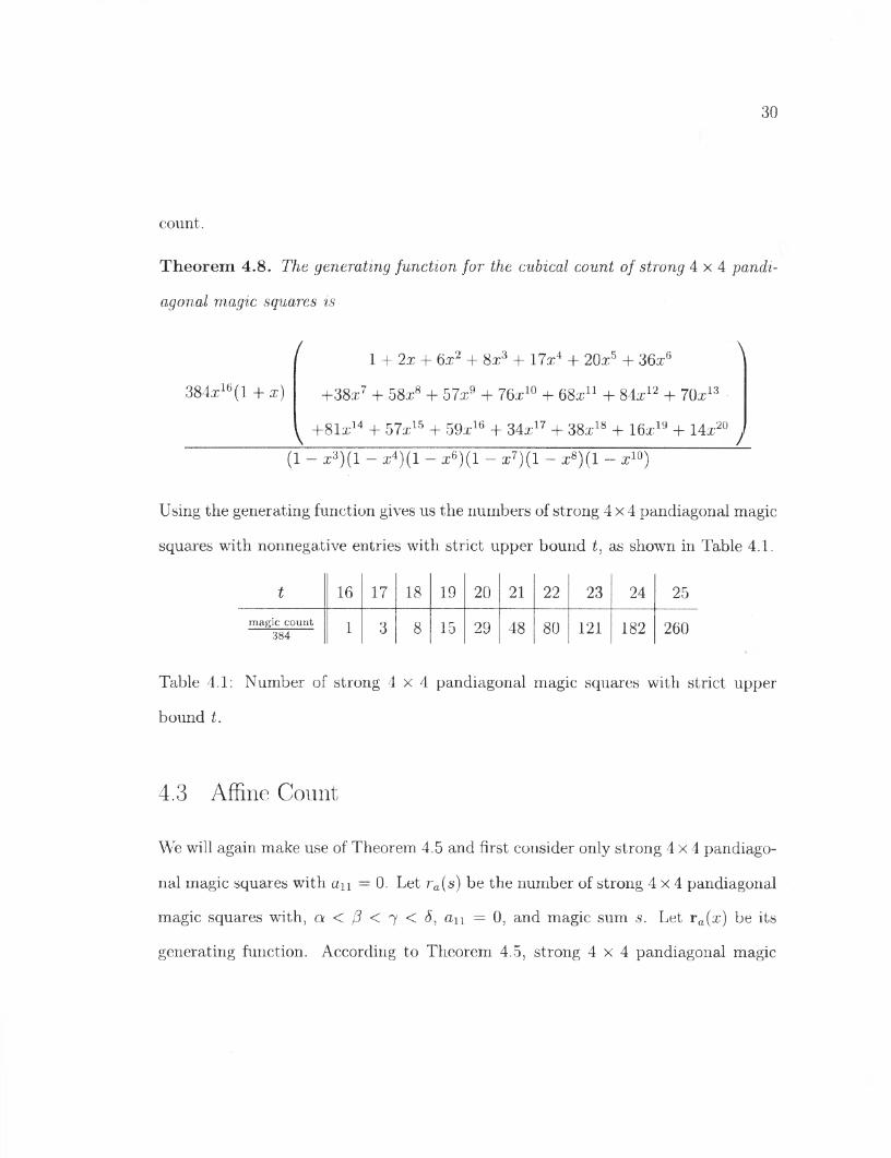
Theorem 4.8. The generating function for the cubical count of strong 4 x 4 pandi

agonal magic squares is

384a;16 (1 + x )

/ 1 + 2x + 6x2 + 8 a;3 + 17a;4 + 20a;5 + 36a;6

+38a;7 + 58a;8 + 57a;9 + 76a;10 + 6 8a;11 + 84a;12 + 70a;13

+81x14 + 57a;15 + 59a;16 + 34a;17 + 38a;18 + 16a;19 + 14a;20

\

(1 — x3) ( l — a;4) ( l — x6)( l — a;7)( l — a;8) ( l — a;10)

Using the generating function gives us the numbers of strong 4 x 4 pandiagonal magic

squares with nonnegative entries with strict upper bound t, as shown in Table 4.1.

t 16 17 18 19 2 0 21 22 23 24 25magic count

384 1 3 8 15 29 48 80 121 182 260

Table 4.1: Number of strong 4 x 4 pandiagonal magic squares with strict upper

bound t.

4.3 Affine Count

We will again make use of Theorem 4.5 and first consider only strong 4 x 4 pandiago

nal magic squares with an = 0. Let ra(s) be the number of strong 4 x 4 pandiagonal

magic squares with, a < /3 < 7 < 6, an = 0, and magic sum s. Let ra(a;) be its

generating function. According to Theorem 4.5, strong 4 x 4 pandiagonal magic

31

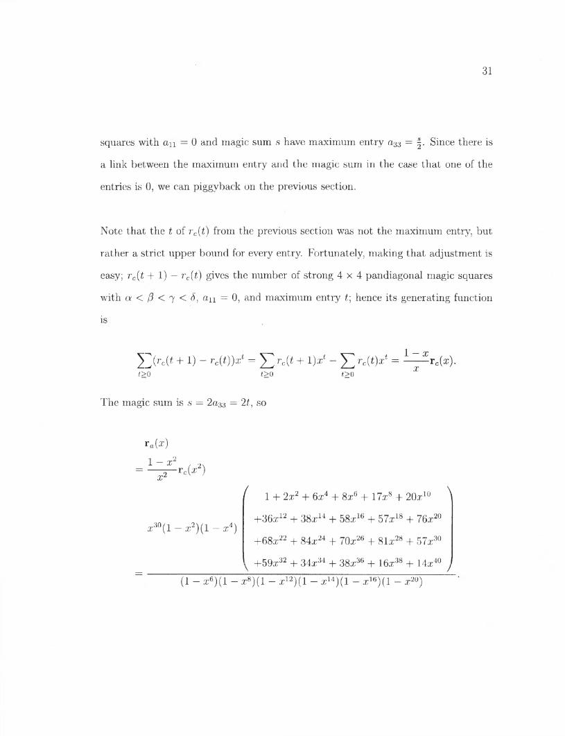
squares with an — 0 and magic sum s have maximum entry a33 = Since there is

a link between the maximum entry and the magic sum in the case that one of the

entries is 0 , we can piggyback on the previous section.

Note that the t of rc(t) from the previous section was not the maximum entry, but

rather a strict upper bound for every entry. Fortunately, making that adjustment is

easy; rc(t + 1) — rc(t) gives the number of strong 4 x 4 pandiagonal magic squares

with a < < 7 < S, an = 0 , and maximum entry i; hence its generating function

is

5 ^ (rc(i + 1) - rc(t))xt = ^ 2 rc(t + 1 )®* - ^ rc(t)x't> 0 t>0 t> 0

X

The magic sum is s = 2 a33 = 21 , so

ra(®)1 — x 2

x2 rc(®2)

a;30(l — a;2) ( l — x4)

1 + 2a;2 + 6a;4 + 8a;6 + 17a;8 + 20a;10 ^

+36x12 + 38a;14 + 58a;16 + 57a;18 + 76a;20

+68a;22 + 84a;24 + 70a;26 + 81a;28 + 57a;30

+59a;32 + 34a;34 + 38a;36 + 16a;38 + 14a;40 y(1 - a;6)(l - a;8)(l - a;12)(l - a;14)(l - a;16)(l - a;20)

32

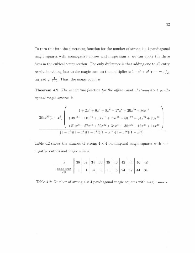
To turn this into the generating function for the number of strong 4 x 4 pandiagonal

magic squares with nonnegative entries and magic sum s, we can apply the three

fixes in the cubical count section. The only difference is that adding one to all entry

results in adding four to the magic sum, so the multiplier is 1 -I- x 4 + x 8 H =

instead of Thus, the magic count is

Theorem 4.9. The generating function for the affine count of strong 4 x 4 pandi

agonal magic squares is

384a;30 (1 - x2)

1 + 2x2 + 6 x 4 + 8 a;6 + 17a;8 + 20a;10 + 36a:12

+38o;14 + 58a;16 + 57a;18 + 76a;20 + 68a;22 + 84a;24 + 70a;26

+81a;28 + 57a;30 + 59a;32 + 34a;34 + 38a;36 + 16a;38 + 14a;40 y

(1 — a;6)(l — a;8)(l — a;12)( l — a;14)(l — a;16)( l — a;20)

Table 4.2 shows the number of strong 4 x 4 pandiagonal magic squares with non

negative entries and magic sum s.

s 30 32 34 36 3 8 40 42 4 4 46 48

magic count 384 1 1 4 3 11 8 24 17 4 4 34

Table 4.2: Number of strong 4 x 4 pandiagonal magic squares with magic sum s.

33

Chapter 5

Strong 5 x 5 Pandiagonal Magic Squares

5.1 Structure

Like the 4 x 4 pandiagonal magic squares, 5 x 5 pandiagonal magic squares have a

nice structure.

Lem m a 5.1. In a 5 x 5 pandiagonal magic square with magic sum s, “+ ” patterns

have sum s. In other words, for any aij, + Otj-i + 1 + ai+i,j — s -

Proof Due to symmetry, it is enough to show a23 + a32 + a33 + a34 + <243 = s.

10s =(an + <125 + a34 + <243 + 52) + (&15 + a-2i + 32 + <243 + 054)

+ (&12 + O23 + a34 + &45 + a5l) + (a14 + &23 + a32 + 041 + O55)

+ (&21 + a22 + <23 + a24 + 25) + 3(a3i + 032 + 033 + <134 + CI35)

+ (041 + 042 + «43 + a44 + O45) + (a 12 + 0,22 + a32 + a42 + a52)

9

34

+ 3 ( a i 3 + C*23 + ®33 + a 43 + a 53) + (^14 + ^24 + &34 + «44 + &54)

~ ( a 13 + a 24 + a 35 + a 41 + a 52) ~ ( a 13 + °2 2 + a 31 + a 45 + a 54)

~ (O l2 + 021 + ^35 + a42 + ^ 53) — (a 14 + «25 + ^31 + a 42 + &53)-

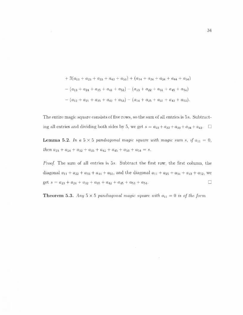
The entire magic square consists of five rows, so the sum of all entries is 5s. Subtract

ing all entries and dividing both sides by 5, we get s = a23 + a32 + a33 + a34 + a43. □

Lem m a 5.2. /n a 5 x 5 pandiagonal magic square with magic sum s, if an = 0,

then a23 + a24 + a32 + a35 + a42 + a45 + 0.53 + W54 = s.

Proof. The sum of all entries is 5 .s. Subtract the first row, the first column, the

diagonal an + 022 + ®33 + a44 + 055, and the diagonal an + a25 + a34 -I- a43 + u.52, we

get s = a23 + a24 + 032 4- 035 4- a42 4- a45 4- 053 4- as4. □

Theorem 5.3. Any 5 x 5 pandiagonal magic square with an = 0 is of the form

35

0 « 3 + 0 1 a 4 + 0 4 Oi 2 + 0 2 Oil + 0 3

a:4 + 0 2 a 2 + 0 3 a 1 01 <*3 + 0 4

a i + 0 i 0 4 Otz + 0 2 a 4 + 0 3 a 2

a 3 + 0 3 Q!4 a 2 + 0 i Cll + 0 4 0 2

OL‘2 + 0 4 + 0 2 0 3 &3 Q?4 + 01

f o r s o m e a i , a 2 , a 3 , a 4 , 0 i , 02, 0s, 0 4 € Z > 0 .

Proof. Let a23 = « i , a24 = 0i, 035 = <2, a45 = 02, a54 — o:3, O53 = 03, a42 = a4,

and a32 = 0±. The row sum an + ai2 + ai3 + au + a^ equals the “+ ” pattern sum

054 + « i3 + a14 + ais + a24, which implies ai2 = a3 + 0i. Equating row/column sums

with “+ ” pattern sums as such gives us the entries of the first row and the first

column in terms of <x,’s and 0$ s. Lemma 5.2 tells us magic sum s = q?i + « 2 + ct3 +

014 + 0 i + 0 2 + 0 3 + 0 4 , so the rest of the entries can be filled out using the “+ ”

patterns. □

36

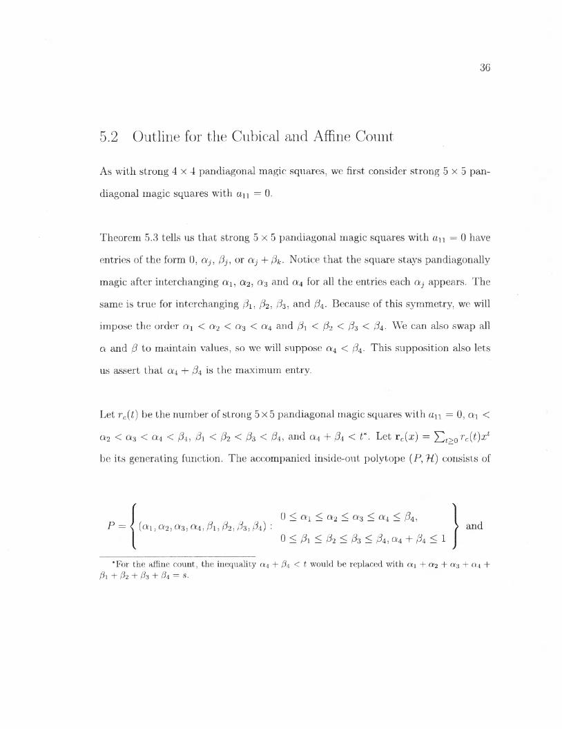
5.2 Outline for the Cubical and Affine Count

As with strong 4 x 4 pandiagonal magic squares, we first consider strong 5 x 5 pan

diagonal magic squares with an = 0 .

Theorem 5.3 tells us that strong 5 x 5 pandiagonal magic squares with an = 0 have

entries of the form 0 , a3, fl3, or a3 + flk. Notice that the square stays pandiagonally

magic after interchanging cti, 0:3 and a4 for all the entries each a3 appears. The

same is true for interchanging /3i, /i2, 1%, and /34. Because of this symmetry, we will

impose the order a,\ < a 2 < 013 < a 4 and (3\ < (i2 < /33 < fa. We can also swap all

a and /3 to maintain values, so we will suppose a 4 < fa. This supposition also lets

us assert that a 4 -I- fa is the maximum entry.

Let rc(t) be the number of strong 5x5 pandiagonal magic squares with an = 0, ai <

a 2 < a 3 < a4 < fa, Pi < P2 < P3 < @4 , and a4 + p4 < t*. Let rc(x) = J2t>0 rc(t)x*

be its generating function. The accompanied inside-out polytope (P, TL) consists of

*For the affine count, the inequality a 4 + /?4 < t would be replaced with « i + + <*3 + a 4 +

P = \ (<*l,Ot2 , 013, a 4, A , P2 , 03, P4 ) '■0 < a i < ol-2 < 013 < 014 < f t ,

0 < Pi < 02 < Pz < P4 , Oi4 + f t < 1

ftl + 02 + @3 + Pi — 5.

37

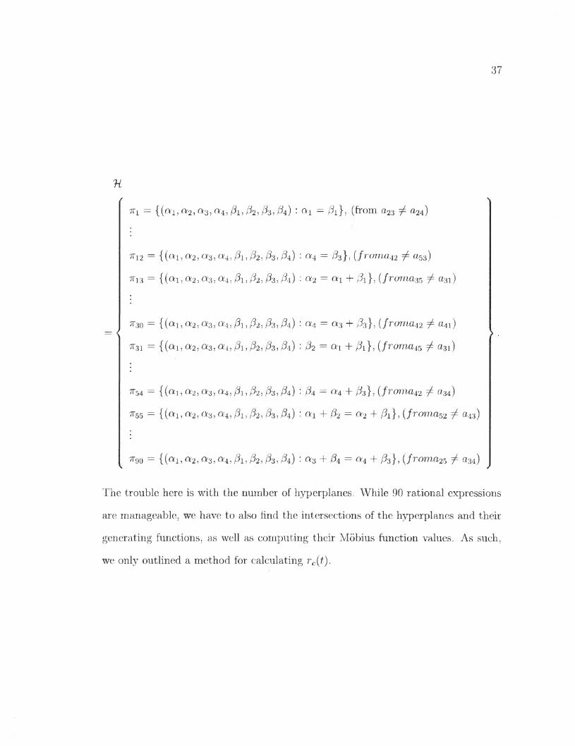
n

7Ti = {(cvi,q;2,Q:3,«4, P i , f a f o , P*) ■ a i = P i } , (from a23 7 a24)

7T12 = {(ai,0i2 ,a3,a 4,pi,p2,p3,p4) : <x4 = Pa}, (from a42 ^ a53)

^ 1 3 = { (a i, Q!2,a 3, 0 :4 , Pi, P2 , P3 , Pa) : a 2 = cci + /?x}, (from a35 ^ a31)

= < .*30 = {(ai, « 2, a3, «4, Pi,P2, Ps, Pi) ■ Oi4 = a .3 + & }, (froma42 a41)

7T3i = {(a i,a 2,a3,a4,/3i,#2,#5,/34) : p2 = cxi + Pi},(froma45 f a31)

7T54 = { ( « i , a2, 0L3 , 014, Pi,P2 , P3 , Pa) ■ Pi = a4 + & } , (.froma42 ^ a34)

7T55 = { ( « 1 , « 2, a3, a 4, Pi,P2 , P3 , Pi) ■ Oil + p2 = a 2 + f t } , (froma52 ± a43)

TTgo = {(ai, 0 2 , «3, « 4, A , P2 , P3 , Pi) ■ «3 + Pa = a4 + f t } , (froma25 ± a34)

The trouble here is with the number of hyperplanes. While 90 rational expressions

are manageable, we have to also find the intersections of the hyperplanes and their

generating functions, as well as computing their Mobius function values. As such,

we only outlined a method for calculating rc(t).

38

Chapter 6

Weak 2 x n Magic Rectangles

Shifting our attention from pandiagonal magic squares to weak 2 x n magic rect

angles, we need to address a few matters. First, row sums cannot equal to column

sums for n ^ 2 , since if they are both s, then the sum of all entries would be both

2 s and ns. Therefore, instead of having a unified magic sum, a rectangular array

qualifies as magic if all row sums are equal and all column sums are equal. Second,

we will focus on the affine count, which will be based on the column sum.

6.1 Weak 2 x 2 n Magic Rectangles

Given a column sum s, the first row of a 2 x 2n magic rectangle has sum ns and

uniquely determines the entries of the second row. Since each a - is nonnegative and

must sum with the entry above or below, each is bounded by s. As such, we

need to count the number of ways for the sum an + • • • 4- a12n to equal ns where

39

a,ij are nonnegative integers less than or equal to s. For simplicity of notation, we

will relabel a\j as aj.

Consider the series ]Caj >oa'<*1+ +a2"- The coefficient of x ns is the number of ways

the sum X^j=i aj *s ns- Let [xk} f (x ) denote the coefficient of x k of the series f (x ) .

This definition allows us to phrase the following theorem.

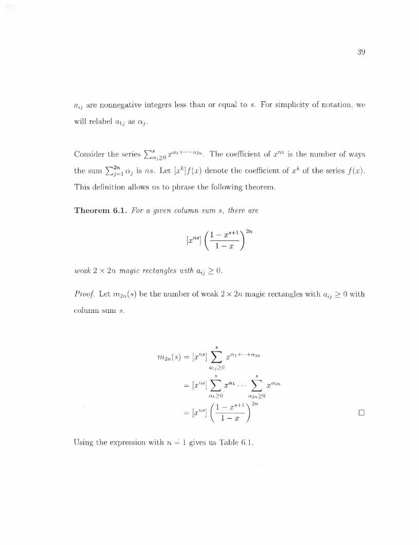
Theorem 6 .1 . For a given column sum s, there are

weak 2 x 2 n magic rectangles with a,ij > 0 .

Proof. Let 7n2n(s) be the number of weak 2 x 2n magic rectangles with al3 > 0 with

column sum s.

ra2n(s) = [:rns] xai+~+a2naij >0

s srOL2n= (!“] £ ■■ • E

« 1>0 «2n 0

/ I - x s+1 \ 2n = 1*1 (— )

Using the expression with n = 1 gives us Table 6 .1 .

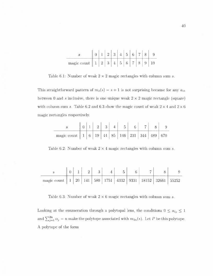
40

s 0 1 2 3 4 5 6 7 8 9

magic count 1 2 3 4 5 6 7 8 9 10

Table 6 .1 : Number of weak 2 x 2 magic rectangles with column sum s.

This straightforward pattern of m2 (s) = s + 1 is not surprising because for any an

between 0 and s inclusive, there is one unique weak 2 x 2 magic rectangle (square)

with column sum s. Table 6 .2 and 6.3 show the magic count of weak 2 x 4 and 2 x 6

magic rectangles respectively.

s 0 1 2 3 4 5 6 7 8 9

magic count 1 6 19 44 85 146 231 344 489 670

Table 6 .2 : Number of weak 2 x 4 magic rectangles with column sum s.

■S 0 1 2 3 4 5 6 7 8 9

magic count 1 20 141 580 1751 4332 9331 18152 32661 55252

Table 6.3: Number of weak 2 x 6 magic rectangles with column sum s.

Looking at the enumeration through a polytopal lens, the conditions 0 < ay < 1

and ]>2j=i aj = n m^ke the polytope associated with rn-inis). Let P be this polytope.

A polytope of the form

41

{(x \ ,. . . , Xd) : 0 < Xj < 1 and xi + ■ ■ ■ + x j = k}

where A: is a positive integer is called a (d, fc)-hypersim plex [5]. With this defini

tion, P is a (2 n, n )-hypersimplex.

Recall from Chapter 3 that the Ehrhart quasipolynomial has degree equal to the

dimension of P, which is 2n — 1 due to the sum equation i aj = n-

The period of m2n(s) divides the least common denominator of the coordinates of

all vertices of P, so we need to know what the vertices of P are.

Theorem 6 .2 . Let P € R2n be the polytope defined by 0 < atj < 1 and Y?jL\ aj = n>

and let V be the set of all 2n-dimensional points where n of the coordinates are ones

and the other n of the coordinates are zeroes. Then P is the convex hull of the points

in V.

This is a known theorem, but we will provide an alternative proof because we can ap

ply the same technique in the 2n+ 1 case. Also, we will use Lemma 6 .6 in Chapter 7 .

Before we begin the proof, we need the four following lemmas.

—4Lem m a 6.3. If a = (ai , . . . , an) and b = (b\,. . . ,bn) have equal coordinates except

for the jth and kth coordinate, and aj + a* = bj + bk, then the convex hull of a and

42

b are points whose nonjth and nonkth coordinates match with a, the jth coordinate

is between a3 and bj, the kth coordinate is between (ik and bk, and the sum of its jth

and kth coordinate is aj + a*..

Proof. For any linear combination kid + k2b where + /c2 = 1 , if a, = 6,, then

A'|Ci.i “j- k‘2bi — kiai ) k2a

Suppose aj > j. Using again ki + k2 — 1 , we get

bj = ktbj + k2bj < kittj + k2bj < k\Oj + k2aj — aj.

If aj + afc = bj + bk, then < bk and bk < k\Ok + k2bk < a . The sum of the two

coordinates of the linear combination is

k\aj + k2bj + k\ak + k2bk — k\ — ki(aj + a ) + k2(bj 4- bk)

= ki(aj + 0 ) + k2(aj + ak)

= (ki + k2)(aj + afc)

= aj + ak- □

As an example, (0 , 1 ,1 ,0 , |) is in the convex hull of (0 , 1 , 1 , 1 , 0 , 0 ) and (0 , 0 , 1 , 1 , 0 , 1).

Lem m a 6.4. If a point in the convex hull of the points in V (as defined in Theorem

6.2), then the point is still in the convex hull after its coordinates are permuted. In

43

other words, for any permutation s of { 1 , . . . , 2 n}, if (a i,. . . , a2n) is in the convex

hull of the points in V, then so is (as(i), . . . , as(2n))-

Proof. Let s be a permutation of { 1 , . . . , 2n}. Since V is the set of all 2 n-dimensional

points where n of the coordinates are ones and the other n of the coordinates are

zeroes, for any v = (ui , . . . , v2n) in V, the point vs := ( fs(i), . . . , vs(2n)) is also

in V. Therefore, if (a^,. . . ,a2n) = 's 'n the convex hull, then so is

(os(l), • • • , Os(2n)) = vVs- I—I

As an example, if (0 , |, 1 , 1 , 0 , |) is in the convex hull of the points in V, then so is

Lem m a 6.5. All points in the convex hull of the points in V have coordinate sum

n.

Proof. Let Vj = . . . , vji2n) for j = 1 , . . . , (2™) be the points in V. All points in

the convex hull can be represented as

(» )

The coordinate sum is, therefore,

2n C : ) ( 2: ) 2n ( f )

2 2 2 2 k^ n = n - □i~ 1 j —1 j = 1 i= l j —1

44

Lem m a 6 .6 . If d is in the convex hull of a and b, and e is in the convex hull of c—* —

and d, then e is in the convex hull of a, b, and c.

Proof. By the definition of convex hull,

d = kid + k2b and e = k3c + k4d

for some ki, k2, k3, k4 such that 0 < kj < 1 and ki + k2 = k3 + k4 — 1 . Therefore,

e = kik4a + k2k4b + k3c. The coefficients have sum 1 and are bounded by 0 and

1 . □

With these four lemmas, we are ready to prove Theorem 6.2.

Proof of Theorem 6.2. Lemma 6.5 ensures that the convex hull of the points in V

is a subset of P. To prove the theorem, we need to show that P is a subset of the

convex hull of the points in V.

With Lemma 6.3 and 6.4, we have another way to think about the convex hull of

the points in V . Imagine a row of 2 n switches representing the coordinates of a

point, up being 1 and down being 0 (see Figure 6.1).

45

Figure 6.1: The first setting represents 0, the second represents |, and the last

represents 1 .

The points in V have settings where n of the switches are up and n of the switches

are down. Lemma 6.3 and 6.4 allow us to select any two switches and move the

higher one down and the lower one up by the same amount without passing each

other. The resulting point is still in the convex hull. To justify this, suppose in a

point, coordinate otj < ak- By Lemma 6.4, if we swap otj and ak, the new point

is still in the convex hull. We can then apply Lemma 6.3. As it is, we can only

perform this move once, but Lemma 6 .6 allows us to perform this move repeatedly.

With this move, we can show that any point (a i , . . . ,a 2n) in P is in the convex

hull of the points in V. First, we identify the order of a\j and set the n higher

coordinates to up and the n lower coordinates to down. This represents a point in

V, which is in the convex hull. Without loss of generality, suppose £*].<•••< a2n-

This implies we start with the setting in Figure 6.2.

46

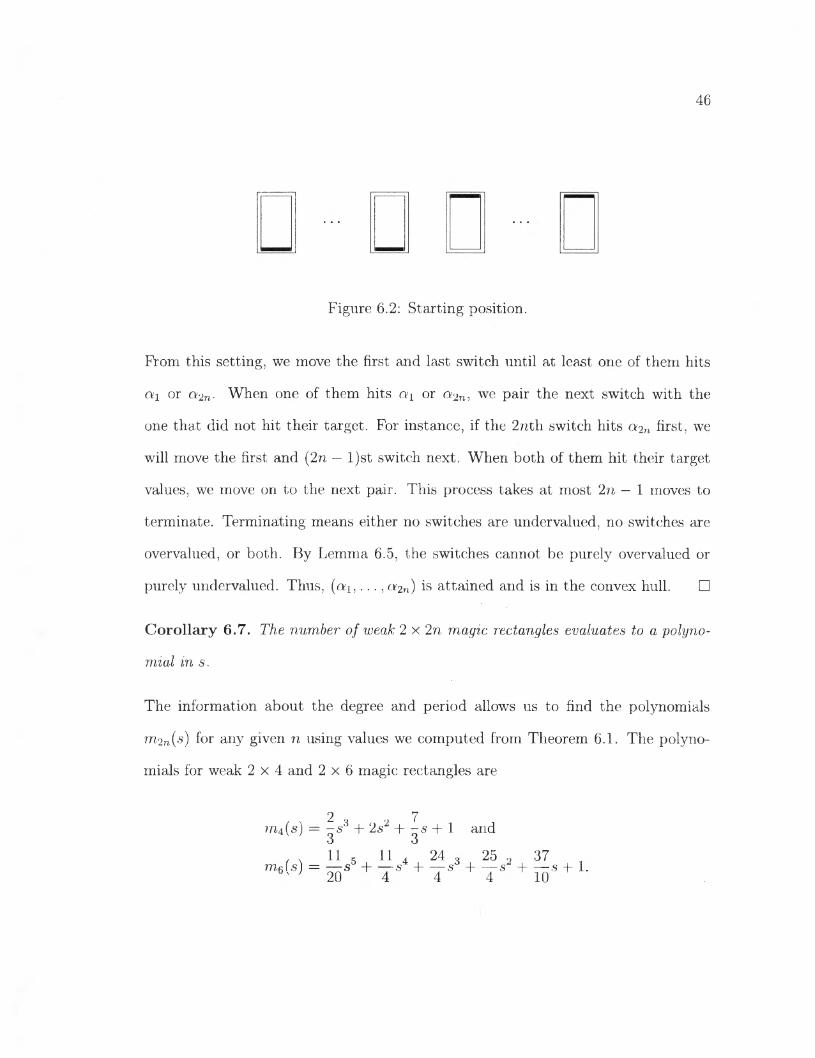
Figure 6 .2 : Starting position.

From this setting, we move the first and last switch until at least one of them hits

c*i or ev2ra. When one of them hits cvi or a 2n, we pair the next switch with the

one that did not hit their target. For instance, if the 2nth switch hits a2n first, we

will move the first and (2n — l)st switch next. When both of them hit their target

values, we move on to the next pair. This process takes at most 2 n — 1 moves to

terminate. Terminating means either no switches are undervalued, no switches are

overvalued, or both. By Lemma 6.5, the switches cannot be purely overvalued or

purely undervalued. Thus, ( a i , . . . , a2n) is attained and is in the convex hull. □

C orollary 6.7. The number of weak 2 x 2 n magic rectangles evaluates to a polyno

mial in s.

The information about the degree and period allows us to find the polynomials

ra2n(s) for any given n using values we computed from Theorem 6.1. The polyno

mials for weak 2 x 4 and 2 x 6 magic rectangles are

?7l4(s)

m6(s)

2 . 7- s 3 + 2 s2 + - s + 1 ando o11 11 24 2 5 o 3 7

20 ■s + T S + T S + Io s + 1

47

6.2 Weak 2 x (2n + 1) Magic Rectangles

In a weak 2 x (2n + 1) magic rectangle with column sum s and row sum r, the sum

of all entries in the whole rectangle is (2 n + l)s = 2 r. Therefore, the column sum

s must be even. We can derive the expression for the magic count the same way as

the previous section.

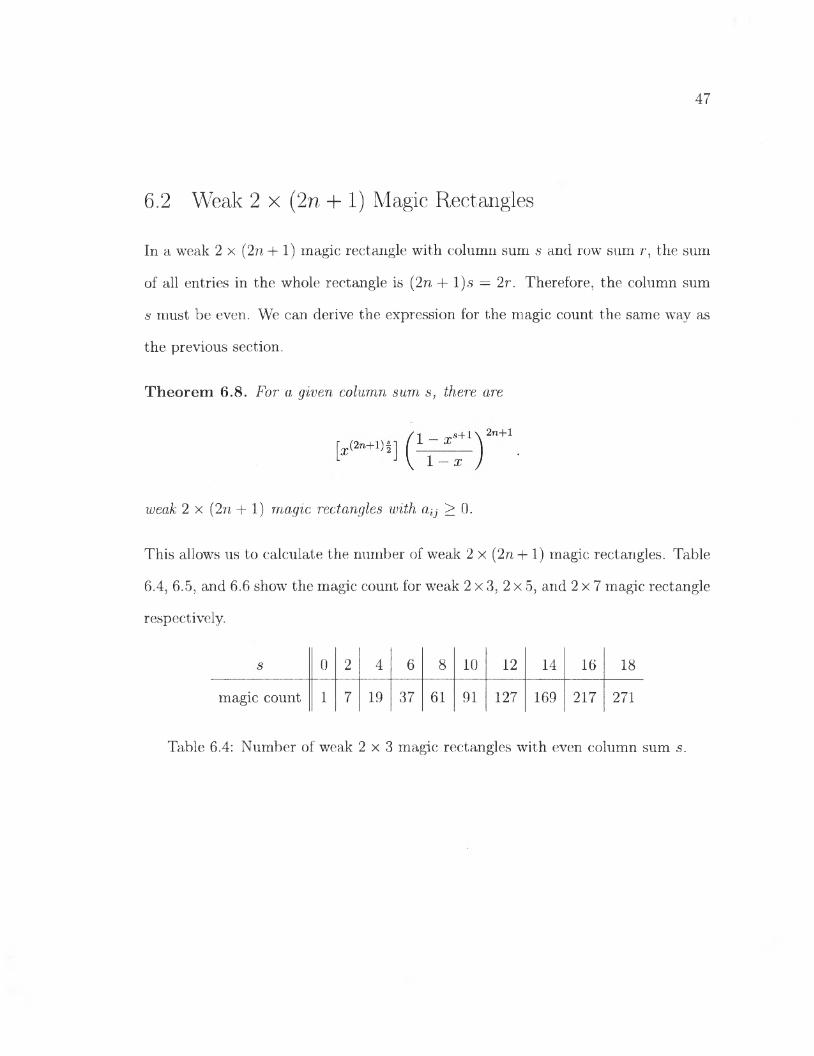
Theorem 6 .8 . For a given column sum s, there are

weak 2 x (2 n + 1 ) magic rectangles with atJ > 0 .

This allows us to calculate the number of weak 2 x (2 n + 1 ) magic rectangles. Table

6.4, 6.5, and 6 .6 show the magic count for weak 2 x 3, 2 x 5, and 2 x 7 magic rectangle

respectively.

s 0 2 4 6 8 10 12 14 16 18

magic count 1 7 19 37 61 91 127 169 217 271

Table 6.4: Number of weak 2 x 3 magic rectangles with even column sum s.

48

s 0 2 4 6 8 10 12 14 16 18

magic count 1 51 381 1451 3951 8801 17151 30381 50101 78151

Table 6.5: Number of weak 2 x 5 magic rectangles with even column sum s.

s 0 2 4 6 8 10 12 14

magic count 1 393 8135 60691 273127 908755 2473325 5832765

Table 6 .6 : Number of weak 2 x 7 magic rectangles with even column sum s.

The polytope associated with the counting quasipolynomial is defined by 0 < atj < 1

Theorem 6.9. The number of weak 2 x (2 n + 1) magic rectangles evaluates to a

quasipolynomial (in s) of period 2 .

Proof. With a similar proof as the previous section, we can show that the polytope

has (2 n + 1 )-dimensional vertices where n coordinates are ones, n coordinates are

zeroes, and one coordinate is The main difference between this polytope and the

(2n, n)-hypersimplex is that is not an integer. This is why, unlike the (2n, n)-

hypersimplex, each vertex of this polytope has a single coordinate being All the

lemmas leading up to the proof of Theorem 6 .2 still apply to this set of points we

49

claim to be the vertices of this polytope.

The least common multiple of the denominator of the vertices is 2 , so the period of

the quasipolynomial divides 2 . The quasipolynomial evaluated at any odd integer s

is 0 because the column sum must be even. Thus, the period of the quasipolynomial

is exactly 2 . □

Just as in the last section, the equation aj ~ cuts down the dimension

by one, and the degree of the quasipolynomial is 2n.

Examples for the quasipolynomials are

|s2 + |s + 1 if s = 0 mod 2 ,m3(s) =

0 if s = 1 mod 2 ;

m5 (s) =

17 17(3 ) =

iMs4 + + 4^52 + f f s + 1 if s = 0 mod 2,

0 if s = 1 mod 2; and

i & 6 + i i « 5 + W s4 + l 53 + W ^ + f ^ + l i f s = ° m°d 2,

0 if s = 1 mod 2 .

50

Chapter 7

2 x n Magilatin Rectangles

The conditions for weak 2 x n magic rectangles as outlined in Chapter 6 still apply

to 2 x n magilatin rectangles, except the magilatin conditions also require entries in

each row/column not to repeat. Due to symmetry, we can rearrange the columns of a

magilatin rectangle such that ai\ < ■ ■ ■ < azn and preserve magilatin ness. Because of

that, we will impose the inequalities ai < ■ ■ ■ < an and multiply the count by n! at

the end. Let magilatin rectangles that satisfy the inequalities be called progressive.

We will first consider 2 x 2n progressive magilatin rectangles. The progressive con

dition solves the issue of repeating row entries. However, if the column sum s is

even, then we have to be careful not to count rectangles with the entry | in order

to avoid duplicate column entries. We will set this caveat aside for a moment.

Let p(M, N, n) denote the number of partitions of n into N parts using the elements

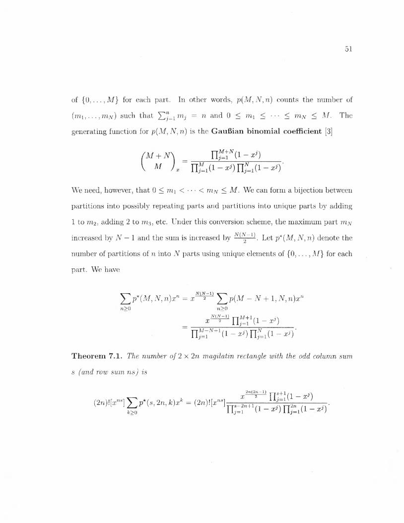
51

of { 0 , . . . , M } for each part. In other words, p(M, N, n) counts the number of

( mi , . . . , wi/v) such that Yl’j= imj = n an< 0 < mi < • • • < mjv < M. The

generating function for p(M, N , n) is the Gaufiian binom ial coefficient [3]

We need, however, that 0 < mi < • • • < uin < M . We can form a bijection between

partitions into possibly repeating parts and partitions into unique parts by adding

1 to m2, adding 2 to m3, etc. Under this conversion scheme, the maximum part mjv

increased by N — 1 and the sum is increased by N N2~1\ Let p*(M, TV, n) denote the

number of partitions of n into N parts using unique elements of { 0 , . . . , M } for each

part. We have

^ p * ( M , N, n )xn = x Y , P ( M ~ N + 1,N, n )xr'i> 0

v~1) r r ^ + 1 /1 i\2 n i=i a - ® 1)

n> 0 n>0mxr') T-rM+1

n ^ +1 ( i - ^ ) n f =i ( i - ^ r

T heorem 7.1. The number o f2 x 2 n magilatin rectangle with the odd column sum

s (and row sum ns) is

^ 2n 2n—1) TTS+Iq _(2n)![a:ns] (s> 2n> *)** = { n)\[xna\, 1 7=1rs—2n+l/ - , t—r2n

fc>0 U s=i

52

This gives us the number of 2 x 2 , 2 x 4, and 2 x 6 magilatin rectangles in Tables

7.1, 7 .2 , and 7.3.

s l 3 5 7 9 11 13 15 17 19magic count

2 l 2 3 4 5 6 7 8 9 10

Table 7.1: Number of 2 x 2 magilatin rectangles with odd column sum s.

s 3 5 7 9 11 13 15 17 19 21

magic count 24 1 3 8 18 33 55 86 126 177 241


s 5 7 9 11 13 15 17 19 21 23magic count

720 1 4 18 58 151 338 676 1242 2137 3486


When the column sum s is even, we need to be mindful about duplicate entries in a

column. Say one of the columns is comprised of two |. Removing the column result

in a 2 x (2n — 1 ) progressive magilatin rectangle with column sum s and row sum

ns — |s. Subtracting the number of such rectangles before multiplying (2n)\ fixes

our count, so let us quickly venture to 2 x (2 n + 1 ) progressive magilatin rectangles.

53

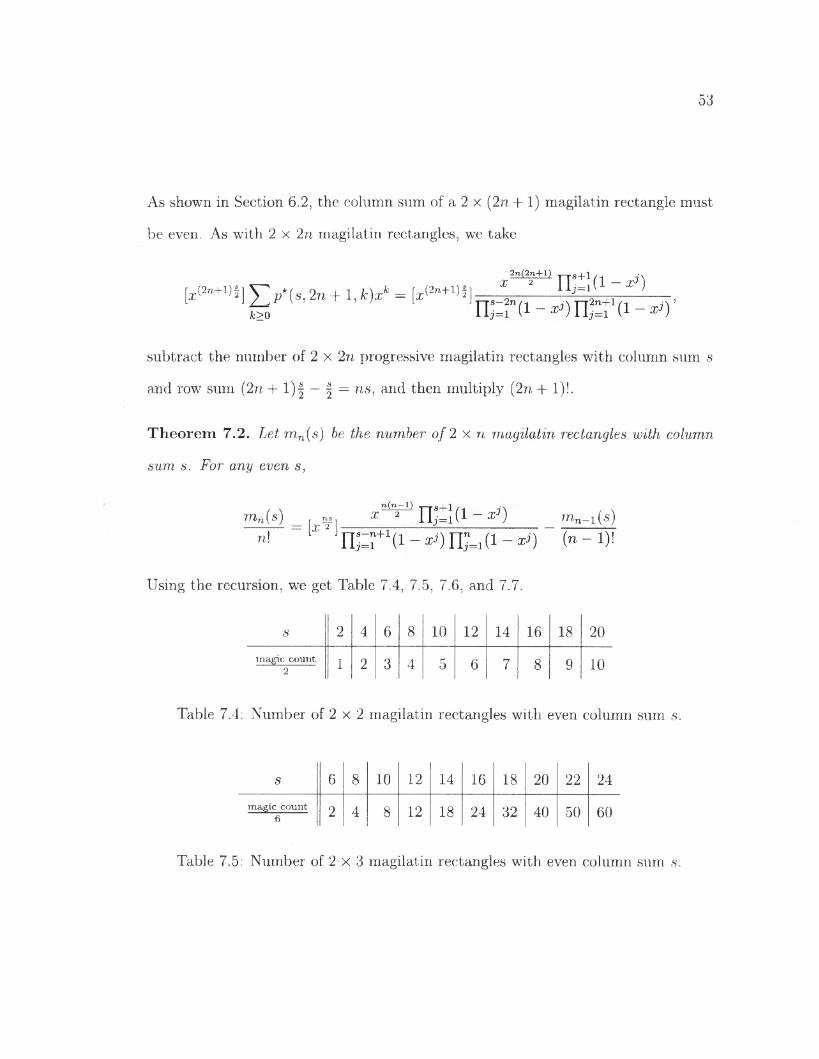
As shown in Section 6 .2 , the column sum of a 2 x (2 n + 1 ) magilatin rectangle must

be even. As with 2 x 2n magilatin rectangles, we take

[ x ^ n y p* (s ,2 n + l ,k )x k = [g (w )S ] * - ■2 n i =lr . ~ x ) ,

subtract the number of 2 x 2 n progressive magilatin rectangles with column sum s

and row sum (2 n + 1 )| — | = ns, and then multiply (2 n + 1)!.

Theorem 7.2. Let mn(s) be the number of 2 x n magilatin rectangles with column

sum s. For any even s,

m n(s)n\ = [** ]:

X__________________________ mw-x(a)

Using the recursion, we get Table 7.4, 7.5, 7.6, and 7.7.

s 2 4 6 8 10 12 14 16 18 2 0

magic count 2 1 2 3 4 5 6 7 8 9 10

Table 7.4: Number of 2 x 2 magilatin rectangles with even column sum s.

s 6 8 10 12 14 16 18 20 22 24

magic count 6 2 4 8 12 18 24 32 40 50 6 0


54

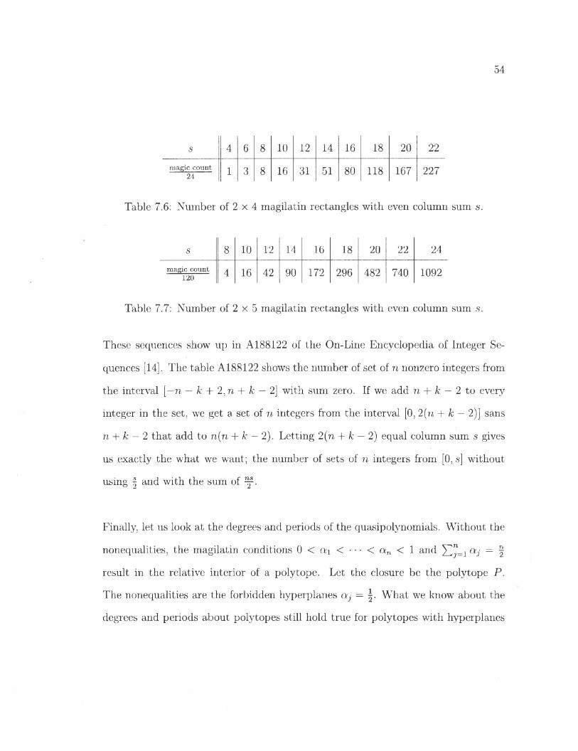
s 4 6 8 10 12 14 16 18 20 22

magic count 24 1 3 8 16 31 51 80 118 167 227


5 8 10 12 14 16 18 20 22 24magic count

120 4 16 42 90 172 296 482 740 1092


These sequences show up in A188122 of the On-Line Encyclopedia of Integer Se

quences [14]. The table A188122 shows the number of set of n nonzero integers from

the interval [—n — k + 2,n + k — 2 ] with sum zero. If we add n + k — 2 to every

integer in the set, we get a set of n integers from the interval [0 , 2{n + k — 2 )] sans

n + k — 2 that add to n(n + k — 2 ). Letting 2(n + k — 2) equal column sum s gives

us exactly the what we want; the number of sets of n integers from [0 , s] without

using | and with the sum of

Finally, let us look at the degrees and periods of the quasipolynomials. Without the

nonequalities, the magilatin conditions 0 < ot.\ < • • ■ < an < 1 and ]Cj=i aj = f

result in the relative interior of a polytope. Let the closure be the polytope P.

The nonequalities are the forbidden hyperplanes aij = What we know about the

degrees and periods about polytopes still hold true for polytopes with hyperplanes

55

removed, but we have to also consider the vertices of the intersections of the poly

tope and the hyperplanes [6 ].

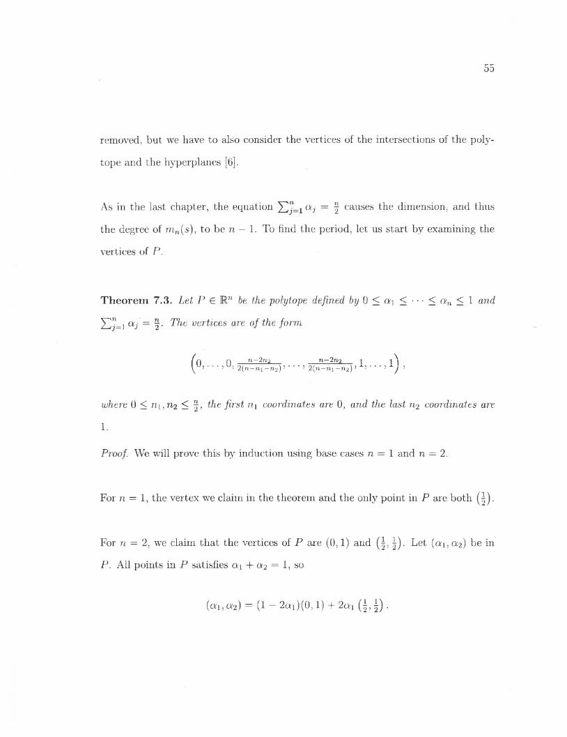
As in the last chapter, the equation ai ~ f causes the dimension, and thus

the degree of mn(s), to be n — 1. To find the period, let us start by examining the

vertices of P.

Theorem 7.3. Let P € Mn be the polytope defined by 0 < « i < • • • < an < 1 and

y;"_i q ? = The vertices are of the form

(n f) __n-2n2__________ 1 1 )y j , . . . ,v , 2(n -n 1-n 2) ’ ‘ * ' ’ 2 (n -n i~ n 2) ’ ’ ' ' ' ’ / ’

where 0 < n\, \ , the first ni coordinates are 0 , and the last n2 coordinates are

1 .

Proof. We will prove this by induction using base cases n — 1 and n = 2 .

For n = 1, the vertex we claim in the theorem and the only point in P are both (| ).

For n = 2 , we claim that the vertices of P are (0,1) and ( 5 , |)- Let (a i,a 2) be in

P. All points in P satisfies ot\ + a 2 = 1, so

(ai, a 2) — (1 — 2 ai ) (0 , 1 ) + 2a.\ (|,

56

Since < a2 and ai + a2 — 1, the coordinate cti must be at most This means

(ai, ct2) is in the convex hull of (0 , 1 ) and (|, |). Also, if k\, k2 > 0 and ki + k2 = 1,

then fci(0 , 1 ) + k2(\, |) satisfies both conditions of P. Therefore, the vertices of P

are (0 , 1 ) and (5 , \).

For the induction step, suppose the polytope P € IRn_2 defined by 0 < c*i < a2 <

■ ■ • < a n - 2 < 1 and aj = ias vertices of the form

( fj fl n—2—2ti2 re—2—2re2 1 i \^U, . . . , U, 2(n -2 -n i -n 2) ’ ' ’ ' ’ 2 ( n - 2 - n i - n 2) ’ ’ ‘ * ' ’ J >

where 0 < n i,n 2 < the first ni coordinates are 0 , and the last n2 coordinates

are 1 . Let V be this set of points. We need to show that the polytope P' € Kn

defined by 0 < a i < a2 < ■ ■ ■ < oin < 1 and J2j=i ai ~ f has vertices of the form

(ft n n-2n2_______ n-2n2_________ i i |y j , . . • , u, 2( n -n i-n 2) ’ ' ‘ * ’ 2( n -n i-n 2) ’ ’ ' ' ' ’ J ’

where 0 < n\, n2 < \ , the first ni coordinates are 0 , and the last n2 coordinates are

1. Let V' be this set of points.

Let (ax, . . . , an) be in P '. We need to first determine if or 1 — an is smaller. If a x

is smaller, we use the point (1 — a n, . . . , 1 — cti) instead, since 0 < a\ < a2 < • ■ ■ <

< 1 if and only i f 0 < l — an < l — a„_i < • - • < 1 — Qfi < 1 ; and oij = | if

57

and only if X™=i(l — an+i-j) = f • Therefore, we can assume 1 — an < c*i without

loss of generality.

We will work backward to prove that ( a j , . . . , an) is in the convex hull of the points

we claimed to be the vertices. First, we will find a point p and coefficients a, b such

that

• a f + b ( \ , . . . ,\ ) = (qi, . . . , otn),

• the last coordinate of p is 1 , and

• a + b = 1 .

From the last coordinate, we get the equation a + = an. Solving it along with

a + b — 1 gives us a = 2an — 1 and b = 2 — 2o;n. Using a and 6 , we have p =

a j = the value of a n is bounded by \ and 1 , and a and b are bounded

by 0 and 1. This means ( a i , . . . , a n) is in the convex hull of p and . . . , .

Furthermore, 0 < < • • • < 1 < 1 and5 — a — — a —

( ai+an- l V a J • • ' i

Qn-l+Qn-a - , l ) . Note that since 0 < a\ < a2 < ■ ■ ■ < an < 1 and

2 an — 12a

n2

58

Now that we pulled the last coordinate to 1, we will find a point q = (q i , . . . ,q n)

and coefficients c, d such that

• ca + d ( ” ~ 2 l) = n — ( ai+a"~x l')cq -t- U ^ 2n-2 > • • • ’ 2 i t -2 ’ V " \ a a ’ l J'

• q\ = 0 , and

• c + d — 1 .

With % = 0 and n2 = 1, the point ( 5^ 5 , • • •, 5^ 3 , l ) is in V'. Using the first

coordinate, we get d = (ai+“ ~ K2n~2) With the assumption earlier that 1 — a n < a l7

the coefficient d must be nonnegative. Also, if a i+ ^ " ~ 1 > then

n 1 171 v—> Gt1 + OLn — 1

2 aj - 1n - l n

= 1 + + ara — 1“ aj=i71—1 n — 2

j=i '

V II — Ji > 1 + ^ 2 ^ 2

= 1 + (n - 1) ” 22n — 2

n2 ’

which is a contradiction. Therefore, 0 < d < 1 , and so is c due to c + d = 1 , imply

ing that (gi±aaid , . . . 5 , l) is in the convex hull of q and • • • > l ) •

Since , 5 ) , ( 2^ ” ■ • • > l) e ^ ^ we can prove that q is in the convex

59

hull of the points in V', then (<*1, . . . , an) is in the convex hull of points in V by

Lemma 6 .6 .

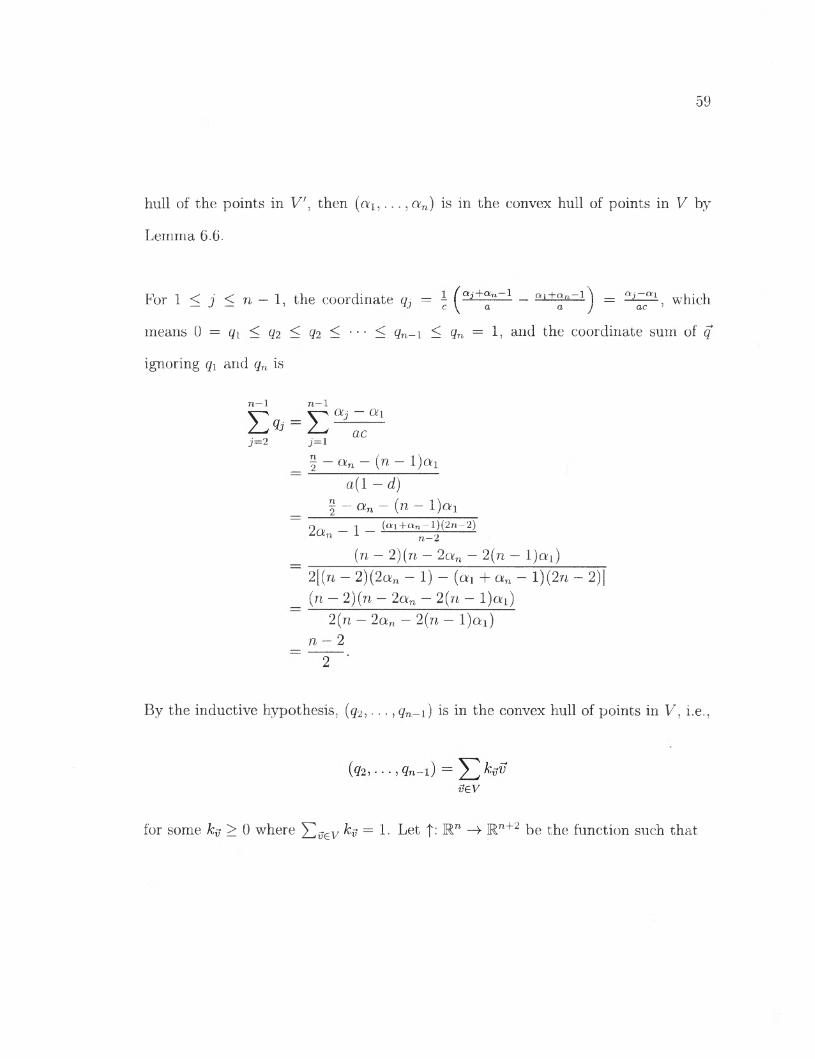
For 1 < j < n — 1, the coordinate qj = - _ « t+are- i \ _ Qj~ai which— J — 1 c V a a J ac 5

means 0 = qi < q2 < q2 < ■ • • < Q n -1 < Qn = 1, and the coordinate sum of q

ignoring q\ and qn is

n—1 n—1Otj — a\

. , acj - 2 j=i_ 2f - an - (n - l ) « i

a (l — d) f - - (n - l )a i

On/ — 1 — (a l + Qn ~ 1) (2n— 2)Z,a’n 1 n—2

(n — 2 ) ( n — 2 a n — 2 (n — l)c i!i )

2 [ (n - 2 ) ( 2 a „ - 1) - ( « i + a n - l ) ( 2 n - 2 )]

(n — 2 )(n — 2an — 2 (n — l)a:i)2 (n — 2 a„ — 2 (n — l )ai )

n — 2

By the inductive hypothesis, (q2, . . . , <7n- i ) is in the convex hull of points in V, i.e.,

v € V

for some > 0 where ]Ci?ev = 1- Let f : R n R n+2 be the function such that

60

t ((®i,.. -, xn)) = (0,x1,..., xn, 1).

If v € V, then t (v) £ V' ■ Therefore,

q = (v)v€V

is in the convex hull of the points in V '. Thus, ( « i , . . . , an) is in the convex hull of

the points in V', finishing the inductive step. □

The hyperplanes we need to remove are of the form

H j (^ -li • • • i CKn) • Oij 2 } •

for j = 1 , . . . , n. No point inside int(P) has | for two coordinates due to strict

inequalities between coordinates, so the hyperplanes do not intersect each other

inside int(P). Let us investigate the vertices of Hj fi P.

T heorem 7.4. Let Qj € Rn be the polytope defined by 0 < c*i < • • • < an < 1 ,

Xw=i aj = and aj = The vertices are of the form

n — n-2 — 2n3 n - n2 - 2n3 1 1 A• * * ? c\( \ 5 ’ * * 5 O ( \ J o ’ * ’ ’ ’ O’ 5 * ’ ’ ’ 1 ^2 (n — rii — n2 — n3) 2 (n — ni — n2 — n3) 2 2 )

1 1 n - n 2 - 2 n 3 n - n2 - 2n3 AU’ , " ,U,2 , ‘ ” , 2 , 2 ( n - n 1 - n 2 - n 3) , ” ' , 2 ( n - n 1 - n 2 - n 3) ’ ’ ■■•’ V ’

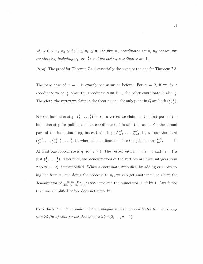
61

where 0 < ni ,n3 < 0 < n2 < n; the first n\ coordinates are 0 ; n2 consecutive

coordinates, including otj, are and the last ro3 coordinates are 1 .

Proo/. The proof for Theorem 7.4 is essentially the same as the one for Theorem 7.3.

The base case of n = 1 is exactly the same as before. For n = 2 , if we fix a

coordinate to be since the coordinate sum is 1 , the other coordinate is also |.

Therefore, the vertex we claim in the theorem and the only point in Q are both (|, |).

For the induction step, (| , . . . , |) is still a vertex we claim, so the first part of the

induction step for pulling the last coordinate to 1 is still the same. For the second

part of the induction step, instead of using • • •, 1 )? we use the point

(^rf, • • • > jr f j !>•••) !> 1)» where all coordinates before the jth one are □

At least one coordinate is |, so n2 > 1 . The vertex with rij = n3 = 0 and n2 = 1 is

just . . . , Therefore, the denominators of the vertices are even integers from

2 to 2 (n — 2) if unsimplified. When a coordinate simplifies, by adding or subtract

ing one from ii\ and doing the opposite to ?i2, we can get another point where the

denominator of n-n^-2ra? -g same an(j the numerator is off by 1. Any factor2{n—n\—ri2— 713J J J

that was simplified before does not simplify.

C orollary 7.5. The number of 2 x n magilatin rectangles evaluates to a quasipoly

nomial (in s) with period that divides 2 lcm(2 , . . . , n — 1).

62

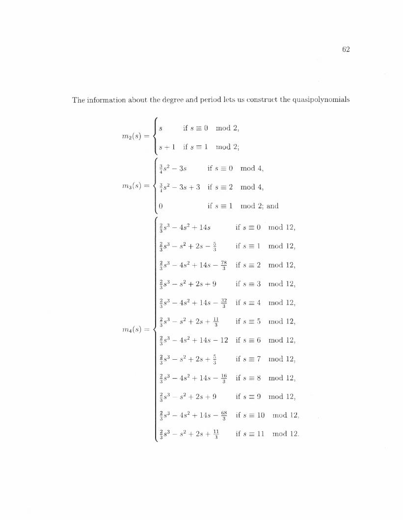
The information about the degree and period lets us construct the quasipolynomials

m2{s) =if s = 0 mod 2,

s + 1 if s = 1 mod 2;

m3(s) -

7B4(s) =

I*2 — 3s if s = 0 mod 4,

I*2 — 3s + 3 if s = 2 mod 4,

0 if s mod 2; and

2S3 — 4s2 + 145 if s = 0 mod 12,

2 3 — s2 + 2s — | if s = 1 mod 12,

— 533 — 4s2 + 14s — 783 if s = 2 mod 12,

2 „33 - s2 + 2s + 9 if s = 3 mod 12,

^5335 - 4s2 + 14s - 323 if s = 4 mod 12,

^533 — s2 + 2s + ^ if s = 5 mod 12,

- 533 — 4s2 + 14s — 12 if s = 6 mod 12,

-,s3 3 5 — s2 + 2s + | if 8 = 7 mod 12,

2 3 35 — 4s2 + 14s — 16

3 if s = 8 mod 12,

?533 - s2 + 2s + 9 if s = 9 mod 12,

-533 — 4s2 + 14s — 683 if s = 10 mod 12,

3 — s2 + 2s + y if s = 11 mod 12.

63

Chapter 8

Cliffhanger (a.k.a. Future Researches)

• In Chapter 5, we did not compute the Ehrhart series for strong 5 x5 pandiag

onal magic squares. If the vertices of the intersections are as nice as the ones

for the 4 x 4 square, then we can write a program for the generating function.

• Strong 6 x 6 may have a nice structure.

• We conjecture that for any integers m and n, the affine count of weak m x mn

magic rectangles follows a polynomial in s, the magic sum, just as the affine

count of weak 2 x 2n magic rectangles.

64

Bibliography

[1] Melencolia I, https://www.nga.gov/collection/axt-object-page.6640.html, March 16th, 2018.

[2 ] Prime Magic Square, http://mathworld.wolfram.com/PrimeMagicSquare.html, March 16th, 2018.

[3 ] George E. Andrews, The theory of partitions, Cambridge Mathematical Library, Cambridge University Press, Cambridge, 1998, Reprint of the 1976 original. MR 1634067

[4] William S. Andrews, Magic squares and cubes, With chapters by other writers. 2nd ed., revised and enlarged, Dover Publications, Inc., New York, 1960. MR 0114763

[5] Matthias Beck and Raman Sanyal, Combinatorial Reciprocity Theorems, AMS, 2018, to appear.

[6 ] Matthias Beck and Thomas Zaslavsky, Inside-out polytopes, Adv. Math. 205 (2006), no. 1 , 134-162. MR 2254310

[7] _______, Six little squares and how their numbers grow, J. Integer Seq. 13 (2010),no. 6 , Article 10.3.8, 45. MR 2659218

[8 ] Alex Bellos, Macau’s magic square stamps just made philately even more nerdy, The Guardian (2014).

[9] Eugene Ehrhart, Sur les polyedres rationnels homothetiques a n dimensions, C. R. Acad. Sci. Paris 254 (1962), 616-618. MR 0130860

https://www.nga.gov/collection/axt-object-page.6640.html

http://mathworld.wolfram.com/PrimeMagicSquare.html

65

[10] Paul A. Gagniuc, Markov chains: From theory to implementation and experimentation., John Wiley Sz Sons, Inc., Hoboken, NJ, 2017. MR 3729435

11] Martin Gardner, Mathematical Games, Scientific American Vol. 249 (1976).

12] Branko Griinbaum, Convex polytopes, second ed., Graduate Texts in Mathematics, vol. 2 2 1 , Springer-Verlag, New York, 2003, Prepared and with a preface by Volker Kaibel, Victor Klee and Gunter M. Ziegler. MR 1976856

13] Brady Haran and Matt Parker, The Parker Square - Numberphile, YouTube, March 16th, 2016.

141 Ronald H. Hardin, The On-Line Encyclopedia of Integer Sequences, A188122, March 16th, 2018.

15] Peter M. Higgins, Number story: From countinq to cryptography, Copernicus Books, New York, 2008. MR 2380416

161 Grasha Jacob and A. Murugan, An integrated approach for the secure transmission of images based on DNA sequences, CoRR a bs /1 6 1 1 .08252 (2016).

17] Ian G. Macdonald, Polynomials associated with finite cell-complexes, J. London Math. Soc. (2 ) 4 (1971), 181-192. MR 0298542

181 Narendra K. Pareek, Design and analysis of a novel digital image encryption scheme, CoRR abs/1204.1603 (2 0 1 2 ).

MAGIC COUNTING WITH INSIDE-OUT POLYTOPES A thesis ...

Documents

Transcript of MAGIC COUNTING WITH INSIDE-OUT POLYTOPES A thesis ...