JHEP03(2007)090

Published by Institute of Physics Publishing for SISSA

Received: March 4, 2007

Accepted: March 9, 2007

Published: March 19, 2007

Counting gauge invariants: the plethystic program

Bo Feng,ab Amihay Hananyc and Yang-Hui Hede

aCenter of Mathematical Science, Zhejiang University

Hangzhou 310027, P. R. ChinabBlackett Lab. & Inst. for Math. Science, Imperial College

London, SW7 2AZ, U.K.cPerimeter Institute

31 Caroline St. N., Waterloo, ON, N2L 2Y5, CanadadCollegii Mertonensis in Academia Oxoniensis

Oxford, OX1 4JD, U.K.eMathematical Institute, Oxford University

24-29 St. Giles’, Oxford, OX1 3LB, U.K.

E-mail: b.feng@imperial.ac.uk, ahanany@perimeterinstitute.ca,

hey@maths.ox.ac.uk

Abstract: We propose a programme for systematically counting the single and multi-

trace gauge invariant operators of a gauge theory. Key to this is the plethystic function.

We expound in detail the power of this plethystic programme for world-volume quiver

gauge theories of D-branes probing Calabi-Yau singularities, an illustrative case to which

the programme is not limited, though in which a full intimate web of relations between the

geometry and the gauge theory manifests herself. We can also use generalisations of Hardy-

Ramanujan to compute the entropy of gauge theories from the plethystic exponential. In

due course, we also touch upon fascinating connections to Young Tableaux, Hilbert schemes

and the MacMahon Conjecture.

Keywords: Differential and Algebraic Geometry, D-branes, Brane Dynamics in Gauge

Theories, AdS-CFT Correspondence.

c© SISSA 2007 http://jhep.sissa.it/archive/papers/jhep032007090/jhep032007090.pdf

JHEP03(2007)090

Contents

1. Introduction and recapitulation 2

2. Explicit expressions for plethystics 4

2.1 All gN as functions of g1 6

2.2 Relation to Young tableaux 7

2.3 Generalising Meinardus 8

2.4 A large class of examples 11

2.5 The entropy of quiver theories 12

3. SU(2) Subgroups: ADE revisited 14

3.1 Recursion relations and difference equations 14

3.2 Full generating functions: MacMahon and Euler 18

3.3 Asymptotic expansions for g∞ 20

3.4 The MacMahon conjecture 21

4. All SU(3) subgroups 22

4.1 The abelian series: Zm × Zn 23

4.2 Non-abelian subgroups 24

4.3 Summary of SU(3) subgroups 25

4.4 The fundamental generating function: the Hilbert series 26

5. Discrete torsion 27

5.1 Example: Z2 × Z2 28

5.2 The general Zn × Zn case 29

6. Hilbert schemes and symmetric products 32

6.1 The second symmetric product of Cm 32

6.2 The n-th symmetric product of C2 34

7. A detailed analysis of Y p,q 34

8. Conclusions and prospects 37

– 1 –

JHEP03(2007)090

1. Introduction and recapitulation

Given a supersymmetric quantum field theory, one of the first quantities one wishes to

determine is the spectrum of BPS operators. Such a desire becomes particularly manifest

for the class of theories which arise in the AdS/CFT correspondence in string theory. Of

special interest are chiral BPS mesonic operators of the 4-dimensional, N = 1 SUSY gauge

theory living on D3-branes probing a Calabi-Yau (CY) singularity. Such a setup has been

archetypal in the aforementioned AdS/CFT correspondence and when the transverse CY

space is trivially C3, we are in the paradigmatic N = 4 CFT and AdS5 × S5 situation of

[1]. When the transverse CY is non-trivial, we have new classes of so-called quiver gauge

theories, pioneered by [2], which has been extensively developed over the past decade (for

a review, q.v. e.g. [3]).

Of vital geometrical significance is the the fact that the BPS mesonic operators form a

chiral ring whose relations determine the transverse Calabi-Yau geometry. More technically,

the syzygy amongst these gauge invariant operators (GIO’s) (modulo F-flatness) gives the

equation of the Calabi-Yau threefold as an affine variety. This correspondence is guaranteed

by the fact, per construtio, the D3-brane probe is a point in the transverse CY. Thus an

intimate relation is established between the gauge theory and the algebraic geometry of

the transverse space.

In our recent paper [4], we solved the problem of counting these mesonic GIO’s for

arbitrary singularities, both single-trace and multi-trace, and for both large and finite

number of D3-branes. Using results from combinatorics, commutative algebra and number

theory, we advocate a plethystic programme wherein such counting problem is not only

systematically addressed, but also intrinsically linked to the underlying geometry. With a

brief recapitulation of this over-arching programme let us first occupy the reader.

To set notation, let a stack of N parallel coincident D3-branes probe a Calabi-Yau

singularity M. The mesonic BPS gauge invariant operators fall into two categories: single-

and multi-trace. The former consists of words in operators, with gauge-indices contracted

but only a single overall trace and the latter, various products of the single-trace GIO’s. We

let the generating function of the single-trace GIO’s be fN (t; M), and that of the multi-

trace be gN (t; M). The n-th coefficient in the power expansion for f and g would then

give the number of GIO’s at level n (where level can be construed as some representative

U(1) charge such as the R-charge, in the problem. For simple cases like Cn or the conifold,

a good U(1) charge is the number of operators, but generically it is not a good qauntum

number and we will refer to a typical U(1) charge). When there are enough isometries,

such as in the case of M being a toric variety, we can refine the counting and extend f and

g to fN (t1, t2, t3; M) and gN (t1, t2, t3; M). Power expansion in the variables t1,2,3 again

gives the number of GIO’s, with the multi-degree now related to global U(1) charges of the

problem, including R-charge and other flavour charges. Some of the main results of [4] are

then as follows.

• The generating functions obey (we can easily generalise from a single variable t to

– 2 –

JHEP03(2007)090

the tuple ti=1,2,3,...):

g1(t) = f∞(t); f∞(t) = PE[f1(t)], g∞(t) = PE[g1(t)]; gN (t) = PE[fN (t)]

where PE is the plethystic exponential function defined as

f(t) =

∞∑

n=0

antn ⇒ g(t) = PE[f(t)] = exp

( ∞∑

n=1

f(tn) − f(0)

n

)=

1∞∏

n=1(1 − tn)an

.

• The quantity f∞ = g1 is the geometric point d’appui and can be directly computed

from properties of M. We have called it the (Hilbert-)Poincare series. In [4], we

referred to this as the Poincare series; it is, in fact, more appropriate, for reasons

which shall become clear in section 4.4, to call it the Hilbert series, an appelation

to which we henceforth adhere. When M is an orbifold C3/G for some finite group

G, f∞ is the Molien series [6] (We remark that Molien series and plethysms have

appeared in the context of four-dimensional dualities in [5]). When M is a toric

variety, f∞ can be obtained from the toric diagram [9] (see also related [20, 21, 46]).

When M is a manifold of complete intersection f∞ can be directly computed by the

defining equations of the manifold.

• The inverse function to PE is the plethystic logarithm, given by

f(t) = PE−1(g(t)) =∞∑

k=1

µ(k)

klog(g(tk)) ,

µ(k) :=

0 k has repeated prime factors

1 k = 1

(−1)n k is a product of n distinct primes

where µ(k) is the Mobius function. The plethystic logarithm of the Hilbert series

gives the syzygies of M, i.e.,

f1(t) = PE−1[f∞(t)] = defining equation of M.

In particular, if M were complete-intersection, f1(t) is a polynomial.

• For finite N , define the function g(ν; t) such that

f∞(t) =

∞∑

n=0

antn ⇒ g(ν; t) :=∞∏

n=0

1(1−ν tn)an =

∞∑N=0

gN (t)νN .

In other words, the ν-expansion of g(ν; t) gives the generating function gN (t) of multi-

trace GIO’s for finite number N of D3-branes. The single-trace generating function

fN (t) is then retrieved from gN (t) by PE−1. This qualifies ν as the chemical potential

for the number of D3-branes.

– 3 –

JHEP03(2007)090

Crucial to the derivation of the above expression is the almost tautological yet very

important fact that

gN (t;M) = g1(t; SymN (M)), SymN (M) := MN/SN .

That is to say, the moduli space of a stack of N D3-branes is the N -th symmetrised

product of that of a single D3-brane, viz., the Calabi-Yau space M.

The above points highlight the key constituents of the plethystic programme and inter-

relates the D-brane quiver gauge theory and the geometry of M. Indeed, one function

distinguishes herself, viz., f∞, which, as a Hilbert series, can be obtained directly from

the geometry. Henceforth, as was in [4], we will often denote the fundamental generating

function f∞ and its associated g∞ simply as f and g.

We emphasise that the applicability of the plethystic programme is not limited to

world-volume theories of D-brane probes on Calabi-Yau singularities. Indeed, if we knew

the geometry of the classical moduli space of a gauge theory, which may not even be N = 1,

and especially if this vacuum space is a complete intersection variety, we could obtain the

Hilbert series and thenceforth use the plethystic exponential to find the gauge invariants.

Without much further ado, let us outline the contents of our current paper. In sec-

tion 2 we derive explicit expressions for the plethystic exponential. We will see how to

recursively write all gN generating functions in terms of the fundamental Hilbert series;

natural connexions with Young tableaux will arise. Of great importantance will also be

the asymptotic behaviour of the multi-trace generating functions gN and we will see how a

result due to Haselgrove and Temperley may be used to generalise the Meinardus theorem.

Thus armed, we can estimate the entropy of our gauge theory; this is the subject of sec-

tion 2.5. We will explicitly see the dependence of the critical exponents on the dimension

of the geometry and the volume of the Sasaki-Einstein manifold.

With all this technology, we move on to concrete classes of examples. In section 3,

we analytically compute the number of single-trace operators for the ADE-singularities

and give the expressions for the asymptotic behaviour of the number of multi-trace opera-

tors. As a passing curiosity, we point out intimate relations to the MacMahon Conjecture.

Then, in section 4, we compute all fundamental generating functions for Calabi-Yau three-

fold orbifolds, again, in explicit detail. Subsequently, one can allow discrete torsion in these

cases, and see how the plethystic programme also encompasses these classes of theories in

section 5. As a mathematical aside, we see how the plethystics relate to Hilbert schemes

of points in section 6. Finally, moving onto toric varieties, we see how the plethystic pro-

gramme lends itself to deriving the equations for wide classes of moduli spaces, exemplifying

with the Y p,q spaces.

2. Explicit expressions for plethystics

With the plethystic programme thus outlined above, it is expedient to present some useful

results concerning the generating functions f and g. First, let us take a closer look at the

– 4 –

JHEP03(2007)090

fundamental relation of the plethystic inversion formula:

g(t) = PE[f(t)] :=PE[

∞∑

k=0

aktk]=exp

∞∑

p=1

1

p(f(tp) − f(0))

=

∞∏

m=1

1

(1 − tm)am⇔

f(t) − f(0) = PE−1[g(t)] =

∞∑

l=1

µ(l)

llog(g(tl)) . (2.1)

The above expression is a central motif for the plethystic programme and the proof of

which was not presented in [4], nor, for that matter, could one find it, within a body of

literature often obscured by mathematical sophistry, in an explicit fashion. The proof is,

in fact, rather straight-forward, which we shall presently see.

Taking the logarithm of the product form of PE in (2.1) and series-expanding, we have

log(g(t)) =∞∑

k=1

(−ak)∞∑

m=1

− 1

m(tk)m . (2.2)

Whence,

PE−1[g(t)] =

∞∑

l=1

µ(l)

llog(g(tl)) =

∞∑

l=1

µ(l)

l

( ∞∑

k=1

ak

∞∑

m=1

1

m(tlk)m

)

=

∞∑

k=1

ak

∞∑

n=1

∑

l|nµ(l)

1

n(tk)n , (2.3)

where we have re-written the double sum on m and l as the alternative sum on n = m l and

its divisors l. Using a fundamental theorem of analytic number theory, viz., the Mobius

inversion formula [10] ∑

d|nµ(d) = δn,1 ,

the double sum∞∑

n=1

(∑l|n

µ(l)

)1n(tk)n simply reduces to tk, whereby making the RHS of

(2.3) equal to∞∑

k=1

aktk = f(t) − f(0), as is required.

Next, the ν-inserted version of PE is of vital importance:

g(ν, t) =∞∏

m=0

1

(1 − ν tm)am=

∞∑

N=0

gN (t)νN . (2.4)

This simple insertion gives us, almost miraculously, the powerful generating functions gN

which capture the multi-trace GIO’s for any finite N and from which the counting fN for

the single-trace GIO’s can be extracted by the plethystic logarithm, i.e., fN = PE−1[gN (t)].

The remarkable fact is that gN (t) requires only the knowledge of the Hilbert series f(t) :=

f∞(t) =∞∑

m=0amtm, which we recall from our outline above, is the fundamental object

obtained purely from the geometry of the Calabi-Yau singularity M. Explicit expressions

fot gN , especially its large-N behaviour, are certainly important in, for example, entropy-

counting of bulk black-hole states.

– 5 –

JHEP03(2007)090

2.1 All gN as functions of g1

Now, from the series expansion (2.4), we can find recursion relations among the coefficients

of expansion, whereby expressing our desired gN in terms of the basic Hilbert series g1 =

f∞. As an enticement, for example, we notice that:

∂2g(ν, t)

∂ν2=

( ∞∑

k=0

aktk

(1 − ν tk)

)2

g(ν, t) + g(ν, t)

∞∑

k=0

akt2k

(1 − ν tk)2,

∂3g(ν, t)

∂ν3=

( ∞∑

k=0

aktk

(1 − ν tk)

)3

g(ν, t) + 3g(ν, t)

( ∞∑

k=0

aktk

(1 − ν tk)

)( ∞∑

k=0

akt2k

(1 − ν tk)2

)+

+g(ν, t)

( ∞∑

k=0

2akt3k

(1 − ν tk)3

).

From this we have

g2(t) =1

2!

∂2g

∂ν2|ν=0 =

1

2[g2

1(t) + g1(t2)] ,

g3(t) =1

3!

∂3g

∂ν3|ν=0 =

1

6[g3

1(t) + 3g1(t)g1(t2) + 2g1(t

3)] . (2.5)

A Systematic Approach: We can obtain the above results more systematically. Re-

calling that the fundamental definition of PE has two equivalent expressions, as a sum or

as a product (q.v. (2.1)), we have that

g(ν, t) =

∞∏

m=0

1

(1 − ν tm)am= exp

( ∞∑

k=1

1

kg1(t

k)νk

), (2.6)

where g1(t) = f∞(t) =∞∑

m=0amtm. Hence,

∞∑

N=0

gN (t)νN = exp

( ∞∑

k=1

1

kg1(t

k)νk

).

Expanding the exponential in the RHS gives a series in powers of ν:

g(ν, t) = 1 + g1(t) ν +

(g1(t)

2 + g1(t2)

)ν2

2+

(g1(t)

3 + 3 g1(t) g1(t2) + 2 g1(t

3))

ν3

6+

+

(g1(t)

4 + 6 g1(t)2 g1(t

2) + 3 g1(t2)

2+ 8 g1(t) g1(t

3) + 6 g1(t4)

)ν4

24+ O(ν5)

Thus, very straight-forwardly, we obtain the expressions for gN (t) by simply reading off the

coeffcients of νN ; giving us the desired generating function gN (t) in terms of the Poincare

series g1 with powers of its argument t. The results for N = 2, 3 are seen to agree with

those in (2.5).

– 6 –

JHEP03(2007)090

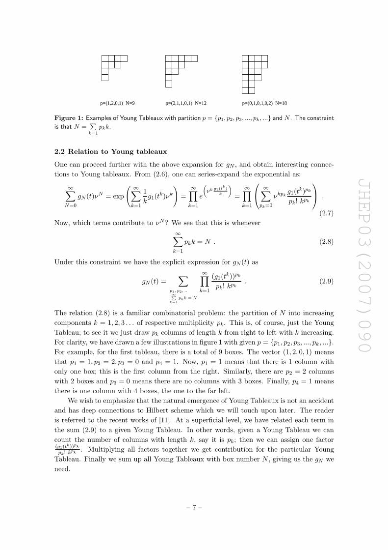
p=(0,1,0,1,0,2) N=18p=(1,2,0,1) N=9 p=(2,1,1,0,1) N=12

Figure 1: Examples of Young Tableaux with partition p = {p1, p2, p3, ..., pk, ...} and N . The constraint

is that N =∑k=1

pkk.

2.2 Relation to Young tableaux

One can proceed further with the above expansion for gN , and obtain interesting connec-

tions to Young tableaux. From (2.6), one can series-expand the exponential as:

∞∑

N=0

gN (t)νN = exp

( ∞∑

k=1

1

kg1(t

k)νk

)=

∞∏

k=1

e

„νk g1(tk)

k

«

=

∞∏

k=1

∞∑

pk=0

νkpkg1(t

k)pk

pk! kpk

.

(2.7)

Now, which terms contribute to νN? We see that this is whenever

∞∑

k=1

pkk = N . (2.8)

Under this constraint we have the explicit expression for gN (t) as

gN (t) =∑

p1, p2, ..∞P

k=1pkk = N

∞∏

k=1

(g1(tk))pk

pk! kpk. (2.9)

The relation (2.8) is a familiar combinatorial problem: the partition of N into increasing

components k = 1, 2, 3 . . . of respective multiplicity pk. This is, of course, just the Young

Tableau; to see it we just draw pk columns of length k from right to left with k increasing.

For clarity, we have drawn a few illustrations in figure 1 with given p = {p1, p2, p3, ..., pk, ...}.For example, for the first tableau, there is a total of 9 boxes. The vector (1, 2, 0, 1) means

that p1 = 1, p2 = 2, p3 = 0 and p4 = 1. Now, p1 = 1 means that there is 1 column with

only one box; this is the first column from the right. Similarly, there are p2 = 2 columns

with 2 boxes and p3 = 0 means there are no columns with 3 boxes. Finally, p4 = 1 means

there is one column with 4 boxes, the one to the far left.

We wish to emphasize that the natural emergence of Young Tableaux is not an accident

and has deep connections to Hilbert scheme which we will touch upon later. The reader

is referred to the recent works of [11]. At a superficial level, we have related each term in

the sum (2.9) to a given Young Tableau. In other words, given a Young Tableau we can

count the number of columns with length k, say it is pk; then we can assign one factor(g1(tk))pk

pk! kpk . Multiplying all factors together we get contribution for the particular Young

Tableau. Finally we sum up all Young Tableaux with box number N , giving us the gN we

need.

– 7 –

JHEP03(2007)090

A Fermionic Version? As a brief digression, one notices that the expression for the

plethstic exponential, in its product form, is a generating function for a bosonic oscillator.

One might wonder what the fermionic counter-part signifies. In other words, we could

define, for f(t) =∞∑

n=0antn,

PE[f(t)] :=∞∏

k=1

(1 + tk)ak , PEν [f(t)] :=∞∏

k=0

(1 + νtk)ak .

It would be interesting to find what these may count in the D-brane gauge theory and

what nice inverse functions they possess.

2.3 Generalising Meinardus

The asymptotic expressions for the generating functions are clearly of importance. In [4],

we discussed at length the so-called Meinardus theorem [12] which generalises the Hardy-

Ramanujan formula for the partition of integers and gives the asymptotics of the function

g∞(t). Now, what about the aymptotic expressions of gN (t) where we have a finite number

N of D3-branes? In other words, we wish to know, as n → ∞ in the expansion

gN (t) =∞∑

n=0

gN (n)tn , (2.10)

the behaviour of gN (n) for a given N .

Thus, we need a generalisation of Meinardus to include ν-insertions. Luckily, there

is a result due to Haselgrove-Temperley [13] with certain relaxation of conditions in [14].

The fermionic version mentioned above has its asymptotics studied in detail by [15]. The

key result of [13, 14] is, under certain convergence conditions into which we shall not delve,

that

THEOREM 2.1. For G(ν, t) =∞∏

r=1(1 − νtλr)−1 =

∞∑n,N=0

gN (n)tnνN , define

Ψ(x) := log G(x) = −∞∑

r=1log(1 − exλr),

K(x) :=∞∏

r=1

(1 + x

λr

)−1ex/λr , F (y) := 1

2πi

i∞∫−i∞

K(x)exydx,

ξ := a root of Ψ′(ξ) + n = 0 , N0 :=∞∑

r=1(eξλr − 1)−1,

then, the asymptotics (for n large and N fixed) are:

gN (n) ∼ ξF ((N − N0)ξ) g(n), g(n) ∼(2πΨ′′(ξ)

)− 12 eΨ(ξ)+nξ .

Of course, we need to recast our g(ν, t) in (2.4) into the form which the theorem

addresses; this is a redefinition of the λr in terms of the am to eliminate repetitions:

λr =

1 r = a0, . . . , a1;

2 r = a1 + 1, . . . , a1 + a2;

3 r = a1 + a2 + 1, . . . , a1 + a2 + a3;

. . .

(2.11)

– 8 –

JHEP03(2007)090

We see that the function G(x) = exp(Ψ(x)) is when the ν-insertion is absent (note

that here counting does start from r = 1) and should capture the original Meinardus result

for the plethystic exponential. Importantly, a key property of Ψ(x), in terms of the am

coefficients (cf. [16]), is that its asymptotic behaviour is

G(x) = eΨ(x) =

∞∏

r=1

(1 − exr)−ar ∼ exp[AΓ(α)ζ(α + 1)x−α − D(0) log x + D′(0)

], (2.12)

where D(s) :=∞∑

m=1

amms is the Dirichlet series which has only 1 simple pole at s = α ∈ R+

with residue A.

Using (2.12) and its derivative, we see that the quantities ξ and g(n) in Theorem 2.1

explicitly evaluate to, for large n,

ξ ∼ Root[−AΓ(α + 1)ζ(α + 1)x−α−1 − D(0)/x + n = 0

]

∼(

1

nAΓ(α + 1)ζ(α + 1)

) 1α+1

(2.13)

g(n) ∼ C1nC2 exp

[n

αα+1 (1 +

1

α) (AΓ(α + 1)ζ(α + 1))

1α+1

]

C1 := eD′(0) 1√2π(α + 1)

(AΓ(α + 1)ζ(α + 1))1−2D(0)2(α+1) , C2 :=

D(0) − 1 − α2

α + 1.(2.14)

We see that g(n) above is exactly the Meinardus result [12, 16] for the asymptotics of the

plethystic exponential without ν-insertion (cf. also, Section 6 of [4]). In other words, the

content of Theorem 2.1 is that the pre-factor

ξF ((N − N0)ξ) (2.15)

encodes the effects of ν-insertion, i.e., the N -dependence, to the classical Meinardus asymp-

totic formula for g(n) in (2.14). For values of n < N the expression for gN (n) should

coincide precisely with that of g∞(n) as the pre-factor tends to 1. On the other hand, for

n > N there will be corrections and the gN (n) is expected to be smaller than g∞(n); this

is because the counting should be less at finite N since there are constraints which vanish

at infinite N .

Example: C Let us first check a simple case. Let am = 1 for all m ∈ Z≥0. This is

where the Hilbert series is equal to f∞(t) = (1 − t)−1 and we recall [4] that the geometry

is just C. The conversion (2.11) makes λr = r, which is a specific example considered on

p238 of [13], giving us

K(x) =

∞∏

r=1

(1 +

x

r

)−1ex/r = eγxΓ(x + 1), F (y) = exp

(−(γ + y) − e−(γ+y)

),

– 9 –

JHEP03(2007)090

where γ := limn→∞

(n∑

j=1j−1 − log(n)

)is the Euler constant1. The Dirichlet series is here

D(s) =∞∑

m=1m−s = ζ(s); whence α = A = 1 with D(0) = −1

2 and D′(0) = −12 log(2π).

Therefore, (2.12) dictates that

Ψ(x) ∼ π2

6x+

1

2log x − 1

2log 2π ⇒ Ψ′(x) ∼ − π2

6x2+

1

2x, Ψ′′(x) ∼ π2

3x3− 1

2x2.

By (2.14) we thus have

ξ ∼ −3 +√

24nπ2 + 9

12n∼ π√

6n, g(n) ∼

(2πΨ′′(ξ)

)− 12 eΨ(ξ)+nξ ∼ 1

4√

3neπ√

2n/3 . (2.16)

Indeed, g(n) is exactly the famous Hardy-Ramanujan asymptotic behaviour for the η-

function. The effect of the ν-insertion is then apparent in the pre-factor governed by the

function F . Now, we see that, for small x,

N0(x) =∞∑

r=1

(exp(rx) − 1)−1 ∼1/x∑

r=1

1

rx+

∞∑

r=1/x

exp(−rx) = −H(1/x)

x+

ex−1

ex − 1∼ − log x

x,

(2.17)

where we have series-expanded for the first part of the sum (H(x) is the Harmonic number)

and neglected the small contribution of the −1 in the denominator for the second sum.

Therefore, since n is large, we can apply (2.17) to give us

N0 = N0(ξ) ∼√

6n

πlog

√6n

π.

Thus, we can write the pre-factor in (2.15) (n is large and N is fixed) as

ξF ((N − N0)ξ) ∼ π√6n

exp(−(γ + (N − N0)

π√6n

) − e−(γ+(N−N0) π√

6n))

∼ π√6n

exp

(log

√6nπ − Nπ√

6n− e

log√

6nπ

− Nπ√6n

)∼ exp(− Nπ√

6n−

√6nπ e

− Nπ√6n ) .

In summary, we have the asymptotic expansion of gN (n) as

gN (n; C) ∼ 1

4√

3nexp

(π

√2n

3

)exp

[− Nπ√

6n−

√6n

πe− Nπ√

6n

]. (2.18)

We have actually reproduced a classical result of [17], which is also studied recently in Bose-

Einstein condensates in [18]. Specifically, the above result agrees completely with Eq.(13)

of [18], wherein they have simplified the expression to g(n)√n

exp(−2c exp(xN (n)) − xN (n))

with c =√

23π, g(n) given in (2.16) and xN (n) := cN

2√

n− log(

√n).

1Indeed, we can see this since F (y) =P

n=−1,−2,−3,...

Resz→n

Γ(z + 1)eγz+zy =∞P

n=0

(−1)n

n!e−(n−1)(γ+y) =

e−1/a/a, for a = exp(γ + y).

– 10 –

JHEP03(2007)090

2.4 A large class of examples

Thus emboldened, we may proceed to more examples. Since the plethystic exponential has

a singularity at t = 1 at ν = 1, it is expedient to study contributions of the form

f(t) = f∞(t;M) = g1(t;M) =V3

(1 − t)3+

V2

(1 − t)2+

V1

1 − t+ V0 + O(1 − t) ; (2.19)

we go up to poles of order 3 because M is at most 3-dimensional in the cases of concern.

Physically, V3 can be thought of as the volume of the dual AdS horizon, i.e., the nor-

malised volume of the Sasaki-Einstein manifold (cf. [9, 20 – 22]), and Vi are related to the

components of the Reeb vectors.

It turns out, for what we shall shortly describe in the next section, that we do not need

as refined an attack as Haselgrove-Temperley, but, rather, a leading order analysis. Indeed,

the results of [13] for d > 1 require a regularisation into whose subtleties we presently do

not wish to venture. We shall, instead, follow the saddle-point method in the physics

literature, such as [19]. Indeed we are essentially studying a contour integral

gN (n) =1

(2πi)2

∮

Γν=0

dν

∮

Γt=0

dtg(ν, t)

νN+1tn+1,

which picks up the residues at the poles and the form in (2.19) will be dominant. The

statement, with the same notations as above, is as follows. For both N and n large (note

that Haselgrove-Temperley only requires that n be large),

gN (n) ∼ g(ν0, t0)ν−N−10 t−n−1

0 , where[N + 1 = ν

∂

∂νlog g(ν, t)

]

ν0,t0

,

[n + 1 = t

∂

∂tlog g(ν, t)

]

ν0,t0

. (2.20)

We can first directly evaluate log g(ν, t). From (2.19), we have that

an = V3(n + 1)(n + 2)

2+ V2(n + 1) + V1 + V0δn,0 ⇒

log g(ν, t) = −∞∑

n=0

an log(1 − νtn)

= −V0 log(1 − ν)

+∞∑

k=1

νk

k

[1

2V3Li−2(t

k) + (V2 +3

2V3)Li−1(t

k) + (V1 + V2 + V3)(1 + Li0(tk))

],

where we have used the definition of the Polylogarithmic function Lid(x) =∞∑

n=1

xn

nd . In fact,

for d ∈ Z≤0, these are simply rational functions.

Recall now that we wish to study the behaviour of g(ν, t) near t = 1 and ν = 1. Hence,

we can define t := e−q and ν = e−w and will study the behaviour near q, w → 0. Series

expanding log g(ν, t) and keeping dominant contributions in the inverses of q and w, we

find that

log g(w, q) ∼∞∑

k=1

νk

k

[V0 +

V1

2+

5V2

12+

3V3

8+

V1 + V2 + V3

k q+

2V2 + 3V3

2 k2 q2+

V3

k3 q3

]

– 11 –

JHEP03(2007)090

∼ V3

q3(ζ(4) − ζ(3)w) − (V0 +

V1

2+

5V2

12+

3V3

8) log(w) . (2.21)

We are now ready to solve for the saddle points given in (2.20). Since t = e−q, ν = e−w,

we have t ∂∂t = − ∂

∂q and ν ∂∂ν = − ∂

∂w and the saddle equations read:

n + 1 = −∂ log g(w, q)

∂q∼ 3ζ(4)V3q

−4 ,

N + 1 = −∂ log g(w, q)

∂w∼ ζ(3)V3q

−3 + (V0 +V1

2+

5V2

12+

3V3

8)w−1 .

Therefore, the saddle points are

q0 ∼(

3V3ζ(4)

n

)14

, w0 ∼ (V0 +V1

2+

5V2

12+

3V3

8)(N − ζ(3)V3q

−30

)−1(2.22)

These results are encouraging. For V0,1,2 = 0 and V3 = 1, the case was studied in nice detail

in [19]. The expressions in (2.22), to leading order, agree exactly with their Eq. (17-19),

in cit. ibid. Substituting back into (2.20), we conclude that, to leading order,

log gN (n) ∼ log g(ν0, t0) + Nw + nq

∼ C0n34 + C1

[N

N − C2n34

+ log(N − C2n

34

)]; (2.23)

C0 := 3−34 4(V3ζ(4))

14 , C1 := V0 +

V1

2+

5V2

12+

3V3

8, C2 := ζ(3)V

14

3 (3ζ(4))−34 .

Once more, we are re-assured. The first term, which only depends on n, should be the

classical Meinardus result while the second is the pre-factor (2.15) discussed above. We

have done the Meinardus analysis for C3 in [4]; substituting ζ(4) = π4

90 gives us the first

term as 2·234 π

3·1514n

34 , precisely the exponent of p1 in Eq (6.7) of [4].

Another interesting limit to consider is t ∼ 1 and ν ∼ 0. Here, we expand about

q = − log t and ν directly and (2.21) becomes

log g(ν, t) ∼ νV3q−3 , (2.24)

giving us the saddle points q0 ∼ 3N/n and ν0 ∼ (3N/n)3N/V3. Thus,

log gN (n) ∼ 4N

(log(N−1n

34 ) + 1 − 1

4log

27

V3

). (2.25)

Note that in order for ν ∼ 0, we need N ¿ n34 .

2.5 The entropy of quiver theories

Having expounded upon a collection of examples and demonstrated the explicit power of the

Halselgrove-Temperley result as well as saddle-point evaluations in generalising Meinardus,

let us now address a problem of great physical interest. A chief motivation for finding

explicit expressions, in paricular the asymptotic behaviour, of our generating functions

– 12 –

JHEP03(2007)090

is to determine the number of degrees of freedom, i.e., the entropy of the gauge theory.

Indeed, as the Hardy-Ramanujan formula is central to the determining the entropy of the

bosonic critical string, the results presented in the previous section will be essential to that

of D-brane probe theories.

The growth of the number of our mesonic BPS operators in the gauge theory can be

a good estimate for the entropy of the system. More generally, it serves as a lower bound

for the total number of operators in the gauge theory, regardless of whether they are BPS

or not. Thus if we are looking for an underlying black hole entropy, the discussions above

will be greatly pertinent. Specifically, in our context of the gauge theory of N D-branes

probing a geometry M, we can define the entropy SN (n) as

SN (n) = log gN (n) where g(ν, t;M) :=

∞∑

N,n=0

gN (n)tnνN , (2.26)

and we recall that g(ν, t;M) is the ν-inserted plethystic exponential of the Hilbert series

(the fundamental generating function f) of the geometry of M.

Now, we would like to compute critical exponents depending on dimensionality. There-

fore, we need to consider the generalisation of (2.19) to

f(t) =Vd

(1 − t)d+ . . . +

V2

(1 − t)2+

V1

1 − t+ V0 + O(1 − t) . (2.27)

Following the computation performed above, we easily see that the saddle points are (in

the t, ν ∼ 1 limit) now

q0 ∼(

dVdζ(d + 1)

n

) 1d+1

, w0 ∼

V0 +

d∑

j=1

Vj(1 +

j−1∑

i=0

βiζ(−i))

(N − ζ(d)Vdq

−d0

)−1,

(2.28)

where βi are coefficients such that

(n + d − 1

d − 1

):=

d−1∑

i=0

βini . (2.29)

Substituting into the saddle point equation, we find the entropy to be

SN (n) ∼ C0nα + C1

[N

N − C2nα+ log (N − C2n

α)

], (2.30)

where the critical exponent is α = dd+1 and the constants are

C0 = d−d

d+1 (d + 1)(Vdζ(d + 1))1

d+1 ,

C1 = V0 +

d∑

j=1

Vj(1 +

j−1∑

i=0

βiζ(−i)) ,

C2 = ζ(d)V1

d+1

d (dζ(d + 1))−d

d+1 .

– 13 –

JHEP03(2007)090

We remark, upon obtaining a similar expression as (2.25) for ν ∼ 0, that our treatment

gives rise to a critical regime in which there is a cross over between ν ∼ 0 and ν ∼ 1. This

critical regime is given by the order parameter N ∼ nd/d+1 or, alternatively, n ∼ N1+1/d.

When the two sides are of the same order we are in the ν ∼ 1 regime and the number of

operators is controlled by n essentially. When the order parameter is small the number of

operators depends on N .

3. SU(2) Subgroups: ADE revisited

We have, in the above, discussed extensively the various general properties of the generat-

ing functions, the recursions, relations to Young tableaux, and especially the asymptotics.

Now, let us move on to some specific examples. An extensively studied class of CY sin-

gularities are orbifold theories. Of particular mathematical interest has been the local-K3

singularities, viz., C2/G where G is a discrete, finite subgroup of SU(2). Such groups fall

under an ADE-pattern and the quivers are central to the McKay Correspondence.

In [4], we computed the fundamental generating functions, i.e., the Hilbert series g1 =

f∞. We recall that for orbifolds of finite group G, the Hilbert series is computed by the

so-called Molien series

f∞(t;G) = M(t;G) =1

|G|∑

g∈G

1

det(I − tg). (3.1)

A natural question to ask is what explicit expressions can be derived for gN at finite N .

Using the prescription in the previous section, we can readily expand a few terms of (2.7)

to see what we obtain. Take the example of G = D4, the binary dihedral group of order 8,

which was investigated in detail in [4], the Hilbert series is the Molien series

g1(t) = M(t; D4) =1 + t6

(1 − t4)2. (3.2)

Substituting (3.2) into (2.7), we obtain (g0(t) = 1 automatically):

g2(t) =1 − t2 + t6 + t8 − t12 + t14

(1 − t2) (1 − t4)2 (1 − t8),

g3(t) =1 − t2 + 2 t8 + t12 + t18 + 2 t22 − t28 + t30

(1 − t2) (1 − t4)2 (1 − t6) (1 − t8) (1 − t12), . . .

We see that these coefficients quickly become complicated. Nevertheless, the algorithm is

clear and one may extract gN ad libertum.

3.1 Recursion relations and difference equations

Let us entice the reader with some immediately noticeable curiosities for the series-coef-

ficients for the Hilbert (Molien) series for the ADE orbifolds. Take the A-family (where

An−1 := Zn). We recall from [4] that

f∞(t; An−1) =(1 + tn)

(1 − t2)(1 − tn).

– 14 –

JHEP03(2007)090

We see that

f∞(t; A1) = 1 + 3t2 + 5t4 + 7 t6 + 9 t8 + 11 t10 + 13t12 + 15t14 + 17 t16 + 19 t18 + 21 t20 + O(t21)

f∞(t; A3) = 1 + t2 + 3 t4 + 3 t6 + 5 t8 + 5 t10 + 7 t12 + 7 t14 + 9 t16 + 9 t18 + 11 t20 + O(t21)

f∞(t; A5) = 1 + t2 + t4 + 3 t6 + 3 t8 + 3 t10 + 5 t12 + 5 t14 + 5 t16 + 7 t18 + 7 t20 + O(t21)

(3.3)

Thus, for n = 2k even, the pattern of the coefficients is {1, . . . , 1; 3, . . . , 3; 5, . . . , 5; . . .}.In fact, we will now proceed to find analytic expressions for the series-coefficients, i.e.,

the number of single-trace GIO’s, of f∞ for all the discrete, finite subgroups of SU(2).

This indeed places our generating function in full power and provide us with invariants of

arbitrary degree immediately. The reason we can do so is because the Molien series is a

rational function in t and indeed, for any rational function, one could systematically obtain

recursion relations, which can then be solved. It is easiest to start with the exceptionals,

i.e., the E-family, with which we shall commence our illustration.

The E6 Singularity: For E6, we recall from [4] that

f =1 − t4 + t8

1 − t4 − t6 + t10= 1 + t6 + t8 + 2 t12 + t14 + O(t16) :=

∞∑

k=0

aktk . (3.4)

Multiplying through by the denominator gives us

1 − t4 + t8 =∞∑

k=0

aktk −

∞∑

k=4

ak−4tk −

∞∑

k=6

ak−6tk +

∞∑

k=10

ak−10tk (3.5)

=

9∑

k=0

aktk −

9∑

k=4

ak−4tk −

9∑

k=6

ak−6tk +

∞∑

k=10

(ak − ak−4 − ak−6 + ak−10) .

Identifying the coefficients of powers of t, this readily gives us the recursion relation:

ak = ak−4 + ak−6 − ak−10, k ≥ 10 . (3.6)

There should be 10 initial conditions for ak, which could be obtained by matching the 1

as well as the −t4 and t8 terms in the LHS with the various finite sum pieces in the RHS

of (3.5). Alternatively, it is easier to simply read off the first 10 values of ak in the series

expansion in (3.4), giving us

a0,6,8 = 1, else, ak<10 = 0 .

Of course, all linear homogeneous difference equations of this kind can be solved. Upon

substitution of the ansatz ak = tk for some t ∈ C, one obtains the eigen-equation for t which

is simply the denominator 1− t4 − t6 + t10 in (3.4). This has 10 roots: {ωi=0,...,56 ,±i} with

double roots at 1 and −1. Using the usual trick that for each multiple root λ of order m,

there are extra roots kj=1,...,m−1λk, the solution is reaily found to be

ak = (−1)k (c(1) + k c(2)) + c(3) + k c(4) + c(5) cos(k π

3) +

c(6) cos(k π

2) + c(7) cos(

2 k π

3) + c(8) sin(

k π

3) + c(9) sin(

k π

2) + c(10) sin(

2 k π

3) ,

– 15 –

JHEP03(2007)090

with initial constants c(i), i = 1, . . . , 10. Matching these with the 10 initial conditions in

(3.6) gives us the final solution

ak =1

72

[3

(1 + (−1)k

)(1 + k) + 18 cos(

k π

2) + 24

(cos(

k π

3) + cos(

2 k π

3)

)+

+8√

3

(sin(

k π

3) − sin(

2 k π

3)

)], k = 0, 1, . . .

There is an obvious cyclicity of 12 and a12m = 1+ m for m ∈ Z≥0. We will shortly see this

in another guise in section 3.2.

The E7 Singularity: For E7, we have [4] that

f =1 − t6 + t12

1 − t6 − t8 + t14= 1+ t8 + t12 + t16 + t18 + t20 + 2 t24 + t26 + t28 + t30 + 2 t32 +O(t34) ,

giving us the recursion relations

ak = ak−6 + ak−8 − ak−14, k ≥ 14, a0,8,12 = 1, else, ak<14 = 0 . (3.7)

This can be readily solved using the above methods to be, for k = 0, 1, . . .,

ak =1

144

[3

(1 + (−1)k

)(1 + k) + 2 cos(

k π

2)

(27 + 24 cos(

k π

6)+

18

(cos(

k π

4) − sin(

k π

4)

)− 8

√3 sin(

k π

6)

)].

Again, there is an obvious cyclicity of 24 and a24m = 1 + m for m ∈ Z≥0.

The E8 Singularity: For E8, we have that [4]

f =1 + t2 − t6 − t8 − t10 + t14 + t16

1 + t2 − t6 − t8 − t10 − t12 + t16 + t18

= 1 + t12 + t20 + t24 + t30 + t32 + t36 + t40 + t42 + t44 + t48 + t50 + t52 + t54

+t56 + 2 t60 + t62 + O(t64) ,

giving us the recursion relations

ak =−ak−2+ak−6+ak−8+ak−10+ak−12−ak−16−ak−18 k ≥ 18, a0,12 =1, else, ak<18 = 0 .

Again, this can be solved exactly, giving us, for k = 0, 1, . . .,

ak =1

1800

[15

(1 + (−1)k

)(1 + k) + 36

√5(5 − 2

√5)(

sin(2kπ

5) − sin(

3kπ

5)

)+

+36

√5(5 + 2

√5) (

sin(kπ

5) − sin(

4kπ

5)

)+

+10 cos(kπ

2)

(45 + 36

(cos(

kπ

10) + cos(

3kπ

10)

)+ 60 cos(

kπ

6) − 20

√3 sin(

kπ

6)

)].

Once more, there is an obvious cyclicity of 60 and a60m = 1 + m for m ∈ Z≥0.

– 16 –

JHEP03(2007)090

The An Family: Now, let us move on to the infinite families. For, An−1, we have that,

letting f∞(t; An) = (1+tn)(1−t2)(1−tn)

:=∞∑

k=0

aktk,

1 + tn =∞∑

k=0

aktk −

∞∑k=2

ak−2tk −

∞∑k=n

ak−ntk +∞∑

k=n+2

ak−n−2tk

=(a0 + a1t + . . . + an+1t

n+1)−

(a0t

2 + a1t3 + . . . + an−1t

n+1)−

−(a0t

n + a1tn+1

)+

∞∑k=n+2

(ak − ak−2 − ak−n + ak−n−2) tk .

(3.8)

Identifying coefficients of t, we have that

ak = ak−2 + ak−n − ak−n−2, k ≥ n + 2 ; (3.9)

we still need n+2 initial conditions. One is obvious, a0 = 1, the remaining can be obtained

by solving for the system of associated equations above for a1, . . . , an+1.

Now, we could solve this recursion equation, which is rather difficult because of the

determination of these initial conditions. However, in this case, it is far easier to simply

observe the pattern and conclude that

n = odd ak = floor( kn ) + 1

2

(1 + (−1) mod (k,n)

)

n = even ak =(floor( k

n

)+ 1

2 )(1 + (−1) mod (k,n)

) (3.10)

Again, the cyclicities are apparent: for odd n, ak=2βn = 2β and for even n, ak=2βn = 4β+1

for β ∈ Z≥0. We will write these coefficients explicitly later using the MacMahon and

Dedekind functions in section 3.2.

The Dn Family: For the Dn+2 groups, the recursion relation reads

f∞(t; Dn+2) =(1 + t2n+2)

(1 − t4)(1 − t2n):=

∞∑

k=0

aktk, ak = ak−4 +ak−2n−ak−2n−4; k ≥ 2n+4 ,

(3.11)

together with 2n + 4 initial conditions.

Once again, it is easier to directly observe the pattern here. First, we notice that, upon

making the substitution t2 → t, the Hilbert series becomes quite analogous to the A-series.

Indeed, in analogy to (3.3), we find that the coefficients for even n come in periodicity of

order n and that for the k-th period the even coefficients are 2k+1 and the odd coefficients

are 0. We will use this in writing expressions for the generating function in section 3.2.

In summary, we may observe the pattern of the expansion coefficients as:

(1 + tn+1)

(1 − t2)(1 − tn):=

∞∑

k=0

bktk ⇒

bk =1

2

(1 + (−1)k

)+ floor

(1

nmod (k, 2n)

)+ 2floor

(k

2n

). (3.12)

Therefore, upon restoring t → t2, we only have even powers; whence, for all k = 0, 1, . . .,

ak =

{0, k odd;12

(1 + (−1)k/2

)+ floor

(1n mod (k, 4n)

)+ 2floor

(k4n

), k even.

(3.13)

– 17 –

JHEP03(2007)090

3.2 Full generating functions: MacMahon and Euler

Having obtained analytic expressions for the counting of single-trace GIO’s, i.e., the coeffi-

cient of the fundamental generating function f∞, the Hilbert series, we can say something

further about the plethystic exponentials. The expressions for the ADE orbifolds can be

represented as infinite sums. Such sums appear in different counting formulae for integer

partitions under special restrictions. For example, it is not surprising to find that the

multi-trace generating function for C2,

g∞(t; C2) = exp

( ∞∑

n=1

1

n

((1 − tn)−2 − 1

))= 1+2t2 +6t3 +14t4 +33t5 +70t6 + . . . (3.14)

generates the sequence of the number of partitions of n objects with 2 colors [24]. It would

be interesting to find similar results for the ADE series.

Now, we can use an alternative representation for the generating functions such as

(2.4). For the exmaple of C2, we recall that

g(ν; t; C2) =

∞∏

n=0

(1 − νtn)−(n+1).

We note that the coefficients an have a linear piece and a constant piece. This property

turns out to be generic for all 2 dimensional singular manifolds. We will therefore define

two basic functions. First, let the generalized MacMahon function be:

M(ν; t) :=∞∏

n=1

(1 − νtn)−n ; (3.15)

next, let the generalized Dedekind Eta function (in this form it is actually the generalised

Euler function, which differs from the Eta function by the famous factor of t−1/24) be

defined as:

η(ν; t) :=

∞∏

n=0

(1 − νtn)−1 . (3.16)

In terms of these functions we can now rewrite

g(ν; t; C2) = M(ν; t)η(ν; t) .

We now wonder if this form of the expression can be done for the ADE orbifolds due to the

fact that the coefficients an for the Hilbert (Molien) series, as we recall from [4], are always

of a linear and a constant form, corresponding to the functions M and η, respectively. This

turns out to be correct.

Let us look, for example, at the generating function for C2/Z2. We find that

g(ν; t; C2/Z2) =

∞∏

n=0

(1 − νt2n)−(2n+1) ,

which can be easily rewritten as

g(ν; t; C2/Z2) = M(ν; t2)2η(ν; t2) .

– 18 –

JHEP03(2007)090

To proceed with the full A-family, we now use the periodic pattern for the coefficient an

which was obtained above in (3.10), and obtain the following succint expression for the

generating function g(ν, t):

g(ν; t; C2/Z2k) =

k−1∏

j=0

M(νt2j ; t2k)2 η(νt2j ; t2k)

g(ν; t; C2/Z2k+1) =

2k∏

j=0

M(νtj ; t2k+1)

k∏

j=0

η(νt2j ; t2k+1)

Similarly, we can obtain the full-generating function for the D-family:

g(ν, t; C2/D2k) =

2k−3∏

j=0

M(νt2j ; t4k−4)

k−2∏

j=0

η(νt4j ; t4k−4)

g(ν, t; C2/D2k+1) =4k−3∏

j=0

M(νt2j ; t8k−4)22k−2∏

j=0

η(νt4j ; t8k−4)2k−2∏

j=0

η(νt2j+4k−2; t8k−4) .

Finally, for the E-family, as mentioned above we find that each of the Hilbert series

come with a quasi-periodicity of 12, 24, and 60 for E6,7,8, respectively, which can be seen

from the explicit expressions for the coefficients in the various equations for ak given in

the previous subsection. The growth of the coefficients is always linear in these periods.

Furthermore, odd powers never appear. Therefore, one can write vectors of length 6, 12,

and 30, which will denote the starting powers of the coefficients. Explicitly, we have:

vE6 = {1, 0, 0, 1, 1, 0}vE7 = {1, 0, 0, 0, 1, 0, 1, 0, 1, 1, 1, 0}vE8 = {1, 0, 0, 0, 0, 0, 1, 0, 0, 0, 1, 0, 1, 0, 0, 1, 1, 0, 1, 0, 1, 1, 1, 0, 1, 1, 1, 1, 1, 0} .

The generating functions then take the form

g(ν, t; C2/E6) =5∏

j=0

M(νt2j; t12)η(νt2j ; t12)vj

E6

g(ν, t; C2/E7) =

11∏

j=0

M(νt2j; t24)η(νt2j ; t24)vj

E7

g(ν, t; C2/E8) =

29∏

j=0

M(νt2j; t60)η(νt2j ; t60)vj

E8 .

Two curiosities are perhaps worthy of note. First, the periodicities of the coefficients in the

Hilbert series are, respectively, one half the order of the finite groups themselves. Second,

for each of the vectors vE6,E7,E8 above, one can draw a line at the middle, then upon mirror

reflection about this line, a zero is mapped to a one, and vice versa.

– 19 –

JHEP03(2007)090

3.3 Asymptotic expansions for g∞

As was emphasised in [4] as well as the proceeding discussions, the asymptotic behaviour

of g∞ is of great interest. Using the Meinardus Theorem, we can estimate the asymptotic

behaviour for g∞ for the ADE-singularities. Though the expressions for the ak are, evi-

dently, quite involved, the large k behaviour is dominated by the term proportional to k,

which can be directly observed; other eigenvalues have less than unit modulus and decay

ad nullam. We wish to find dm in

∞∏

k=1

1

(1 − tk)ak:=

∞∑

m=0

dmtm

for large m.

It suffices to see the large k behaviour of ak for the ADE-orbifolds. We see, from the

expressions above, that all ak are essentially linear in k. For An−1, n odd, the coefficient

of the linearity is simply 1/n. For all other cases, the coefficient is the reciprocal of 1/2

the order of the group. However, for all these cases, exactly 1/2 of the terms are zero

and contribute 1 to the product. Therefore, overall, the effective large k-behaviour is still

simply the reciprocal of the order of the group. Hence, we conclude that

For G = ADE, ak ∼ k

|G| . (3.17)

Now, we are at liberty to use the Meinardus analysis. For ak ∼ k, we recall from [4]

that this is the case of the MacMahon function, whose behaviour goes as

∞∏

k=1

1

(1 − tk)k:=

∞∑

m=0

ϕ(m)tm, ⇒ ϕ(m) ∼ 2−1136 ζ(3)

736 e

112

Gl

√3π

m− 2536 exp

(3

2(2 ζ(3))

13 m

23

),

(3.18)

with Gl := 112 − ζ ′(−1) being the Glaisha constant. Thus, we see that for G being an

ADE-group,

dm ∼ ϕ(m)1

|G| . (3.19)

In fact, taking the logarithm of this expression will give us the entropy of the quiver gauge

theory as discussed in section 2.5. We conclude that the entropy is reduced by a factor of

|G| and this is the natural expectation from an extensive parameter like the entropy since,

by the orbifold action, we are losing |G| of the degrees of freedom.

Incidentally, the MacMahon function is the generating function for the plane-partition

problem which is a generalisation of the Young Tableaux to 2-dimensions. That is, consider

an integer m, how many ways are there to write

m =∑

i,j

ni,j such that ni+1,j ≥ ni,j, ni,j+1 ≥ ni,j; ni,j ∈ Z+ .

The answer was shown in [25] to be precisely ϕ(m). The 1-dimensional partition problem,

i.e., how many Young Tableaux (also called Ferrers Diagram) are there of a given total

number of squares, is simply the standard partitioning problem. By this we mean how

– 20 –

JHEP03(2007)090

many ways, irrespectively ordering, are there to write a given integer m as sums of integers.

This is because we could always order the parts in decreasing fashion and arrive at a Young

Tableau. The generating function here is simply the famous Euler function∞∏

k=1

1(1− tk)

. It

is a curious fact that 3 and higher dimensional analogues of the problem remain unsolved.

A conjecture was made in [25] which was later shown to be incorrect.

We see that counting GIO’s for the ADE gauge theories is related to the 2-dimensional

counting problem in a simple fashion: generating function, asymptotically, is simply that

of the MacMahon to the |G|-th root. This can be conceived of tiling, asymptotically, not

the whole plane, but rather, a |G|-th fraction of the plane, as the orbifold indeed requires.

However, to which exact partition problems the ADE results correspond remains elusive.

3.4 The MacMahon conjecture

One could imagine what the result for solid-partitions, which, as mentioned above, is

unknown, might actually be. Let us tabulate the result for the gauge theories for C and

C2. We recall from [4] that

f∞(t; C) =1

1 − t=

∞∑

k=0

tk, ⇒ g∞(t; C) =

∞∏

k=1

1

(1 − tk);

f∞(t; C2) =

1

(1 − t)2=

∞∑

k=0

(k + 1)tk, ⇒ g∞(t; C2) =

∞∏

k=1

1

(1 − tk)k+1.

Thus we see that the multi-trace problem for C counts the 1-dimensional partition; that

for C2, when shifted by 1, counts the 2-dimensional problem. It is perhaps natural to

guess that the one for C3, when shifted by one, would give the generating function for the

3-dimensional partition problem, i.e.,

f∞(t; C3) =

1

(1 − t)3=

∞∑

k=0

(k + 1)(k + 2)

2tk, shift ⇒ ak =

k(k + 1)

2⇒ (3.20)

g∞ =

∞∏

k=1

1

(1 − tk)k(k+1)

2

= 1 + t + 4 t2 + 10 t3 + 26 t4 + 59 t5 + 141 t6 + 310 t7 + 692 t8 + O(t9) .

Unfortunately, this leads us back to MacMahon’s erroneous guess [25]. The correct num-

bers, as generated by exhaustive computer simulation of the explicit partitions, should be

(cf. e.g. [26]):

1, 1, 4, 10, 26, 59, 140, 307, 684, 1464, 3122, 6500, 13426, 27248, 54804, 108802, . . . (3.21)

One sees that starting from the term 141, the generating function g∞ in (3.20) over-counts.

The actual series ak which does generate the correct numbers can be easily found, by taking

the plethystic logarithm, to be (cf. also [26])

ak=1,2,... = {1, 3, 6, 10, 15, 20, 26, 34, 46, 68, 97, 120, 112, 23,−186,−496,

−735,−531, 779, 3894, 9323, 16472, 23056, 23850, 10116, . . .} .(3.22)

– 21 –

JHEP03(2007)090

As it is evident, the negative entries complicate things; it suggests that ak itself cannot be a

Hilbert series. Could it be the plethystic logarithm of a Hilbert series? Recall that for these,

there are often negative entries, signifying relations among fundamental invariants. Well,

it certainly is the plethystic logarithm of something; this is after all, how the series (3.22)

was obtained from (3.21), but this brings us to to where we started. What if we took the

plethystic log of (3.22) itself? Unfortunately, we obtain nothing particularly enlightening.

4. All SU(3) subgroups

We have discussed the ADE-groups above in some detail; of perhaps more physical interest

are the orbifolds of C3. These are local Calabi-Yau threefolds that give rise to N = 1

4-dimensional chiral gauge theories on the D3-brane world-volume. The quiver theories

were studied in [23] and using the notation therein, the discrete finite subgroups of SU(3)

are:

(I) The infinite family Zm × Zn;

(II) The infinite families ∆(3n2) and ∆(6n2);

(III) The exceptionals Σ60, Σ108, Σ168, Σ216, Σ648, and Σ1080.

The theory of Molien series and algebraic invariants is nicely exposed in [6], wherein some

explicit Molien series are also computed for the discrete subgroups of SL(3; C).

In order to explicitly write the generators of the groups, first, define

ωn := exp(2πi

n),

and the matrices

S :=

(1 0 0

0 ω3 0

0 0 ω32

), S1 :=

(1 0 0

0 ω54 0

0 0 ω5

), S2 :=

(ω7 0 0

0 ω72 0

0 0 ω74

);

T :=

(0 1 0

0 0 1

1 0 0

), T1 := 1√

5

(1 1 1

2 12(−1 −

√5) 1

2(−1 +

√5)

2 12(−1 +

√5) 1

2(−1 −

√5)

), T2 :=

(1 0 0

0 0 1

0 −1 0

);

R := − 1√−7

(−ω7

3 + ω74 ω7

2 − ω75 ω7 − ω7

6

ω72 − ω7

5 ω7 − ω76 −ω7

3 + ω74

ω7 − ω76 −ω7

3 + ω74 ω7

2 − ω75

);

U :=

(ω9

4 0 0

0 ω94 0

0 0 ω3 ω94

), U1 :=

(−1 0 0

0 0 −1

0 −1 0

);

V := 1√−3

(1 1 1

1 ω3 ω32

1 ω32 ω3

), V1 := 1√

5

(1 1

4(−1 +

√−15) 1

4(−1 +

√−15)

12(−1 −

√−15) 1

2(−1 −

√5) 1

2(−1 +

√5)

12(−1 −

√−15) 1

2(−1 +

√5) 1

2(−1 −

√5)

);

A(m) :=

(ωm 0 0

0 1 0

0 0 ω−1m

), B(n) :=

(1 0 0

0 ωn 0

0 0 ω−1n

).

(4.1)

– 22 –

JHEP03(2007)090

Finally, we adhere to the usual notation that

G = 〈g1, . . . , gk〉

is the finite group G generated by matrices g1, . . . gk.

4.1 The abelian series: Zm × Zn

The first of our series is simply Zm × Zn = 〈A(m), B(n)〉. The Molien series is given by

f(t; Zm × Zn) =1

mn

m−1∑

i=0

n−1∑

j=0

det

(I3×3 − t

(ωi

m 0 0

0 ωjn 0

0 0 ω−im ω−j

n

))−1

(4.2)

=1

mn

m−1∑

i=0

n−1∑

j=0

1

(1 − tωim)(1 − tωj

n)(1 − tω−im ω−j

n )

=1

mn

m−1∑

i=0

n−1∑

j=0

∞∑

p,q,r=0

tpωipmtqωjq

n trω−irm ω−jr

n .

Using the identitym−1∑

i=0

ωixm = mδx,mZ ,

where the Kronecker-Delta is 1 whenever x is a multiple of n, we can see that non-zero

contributions come from

p = r + p m for p = −[r

m],−[

r

m] + 1, . . . ; q = r + q n for q = −[

r

n],−[

r

n] + 1, . . . .

Here, [ rm ] means to take the integer part (i.e., floor(r/m)). Whence,

f(t; Zm × Zn) =

∞∑

r=0

∞∑

ep=−[ rm

]

∞∑

eq=−[ rn

]

t3r+ep m+eq n =

∞∑

r=0

t3r−[ rm

]m−[ rn

]n

(1 − tm)(1 − tn).

To go further, we can write r = r + LCM(m,n)z for z = 0, 1, ...,∞ and r = 0, 1, ...,

LCM(m,n)− 1, where LCM is the lowest common multiple. Using this parametrization,

the sum reduces to

f(t; Zm × Zn) =1

(1 − tm)(1 − tn)

LCM(m,n)−1∑

er=0

∞∑

z=0

t3er−[ erm

]m−[ ern

]ntLCM(m,n)z (4.3)

=1

(1 − tm)(1 − tn)(1 − tLCM(m,n))

LCM(m,n)−1∑

er=0

t3er−[ erm

]m−[ ern

]n .

The above expression becomes particularly simple in the case of perhaps greatest interest,

viz, when m = n; here LCM(m,n) = m and within the range of summation of r, [ erm ] is

zero, hence

f(t; Zm × Zm) =1 − t3m

(1 − t3)(1 − tm)3. (4.4)

– 23 –

JHEP03(2007)090

Taking the plethystic logarithm of (4.4) gives polynomials, suggesting that C3/(Zm ×Zm)

are all complete intersections! Explicitly, we have that

f1(t; Zm × Zm) = PE−1[f(t; Zm × Zm)] =

3t m = 1,

3t2 + t3 − t6 m = 2,

4t3 − t9 m = 3,

t3 + 3tm − t3m m ≥ 4.

(4.5)

The m = 1 case is a good check; this is simply the result for the parent C3 theory.

Refinement: As was pointed out in [4], where there are enough isometries, as certainly

is the case with toric varieties, refinements can be made to the Molien series. The above

Abelian series are indeed toric, hence one could write the refined Molien (Hilbert) series as

f(t1, t2, t3; Zm × Zn) =1

mn

m−1∑

i=0

n−1∑

j=0

det

(I3×3 −

(t1 0 0

0 t2 0

0 0 t3

)(ωi

m 0 0

0 ωjn 0

0 0 ω−im ω−j

n

))−1

.

This can, using the above reparametrisation of the summation variables, be re-written as

f(t1, t2, t3; Zm ×Zn) =1

(1 − tm1 )(1 − tn2 )(1 − tLCM(m,n)3 )

LCM(m,n)−1∑

er=0

(t1t2t3)ert

−[ erm

]m1 t

−[ ern

]n2 .

Once again, for the case of m = n, the expression simplifies considerably:

f(t1, t2, t3; Zm × Zm) =1 − (t1t2t3)

m

(1 − t1t2t3)(1 − tm1 )(1 − tm2 )(1 − tm3 ). (4.6)

The plethystic logarithm of this expression becomes particularly simple:

f1(t1, t2, t3; Zm × Zm) = tm1 + tm2 + tm3 + t1t2t3 − (t1t2t3)m , m = 1, 2, 3, . . . (4.7)

4.2 Non-abelian subgroups

Having expounded upon the Zm × Zn series in detail, we can proceed to the non-Abelian

groups. The Molien series for the exceptionals can be quite simply computed by [28] and

are presented in the next subsection. The two Delta-series maybe dealt with in much the

same manner as the abovementioned Zm × Zm.

The elements of ∆(3n2) := 〈A(n), B(n), T 〉 fall into three classes, viz, the orbits of

Z2n ' 〈A(n), B(n)〉 under {I, T, T 2} since the matrix T , which we recall from (4.1), is of

order 3. Therefore,

f(t; ∆(3n2)) =1

3n2[

n−1∑

i,j=0

det

(I3×3 − t

(ωi

n 0 0

0 ωjn 0

0 0 ω−i−jn

))−1

+det

(I3×3−t

(0 ωj

n 0

0 0 ω−i−jn

ωin 0 0

))−1

+ det

(I3×3 − t

(0 0 ω−i−j

n

ωin 0 0

0 ωjn 0

))−1

]

=1

3n2

[n2 1 − t3n

(1 − t3)(1 − tn)3+ n2 1

1 − t3+ n2 1

1 − t3

]

– 24 –

JHEP03(2007)090

=1 − tn + t2n

(1 − t3)(1 − tn)2. (4.8)

One could in fact take the plethystic logarithm and see that these are complete intersections:

f1(t; ∆(3n2)) = PE−1[f(t; ∆(3n2))] =

t + t2 + 2 t3 − t6 n = 1,

t2 + t3 + t4 + t6 − t12 n = 2,

2 t3 + t6 + t9 − t18 n = 3,

t3 + tn + t2n + t3n − t6n n ≥ 4.

(4.9)

In complete analogy, ∆(6n2) := 〈A(n), B(n), T, T2〉. In fact ∆(6n2) ' ∆(6(2n)2), thus

it suffices to consider only odd n, and we have that

f(t; ∆(6n2)) =1 + t6n+3

(1 − t6)(1 − t2n)(1 − t4n), n = 1, 3, 5, . . . .

Again, taking the plethystic logarithm shows these to be complete intersections

f1(t; ∆(6n2)) = PE−1[f(t; ∆(6n2))] =

t2 + t4 + t6 + t9 − t18 n = 1,

2 t6 + t12 + t21 − t42 n = 3,

t6 + t2n + t4n + t6n+3 − t12n+6 n ≥ 5.

(4.10)

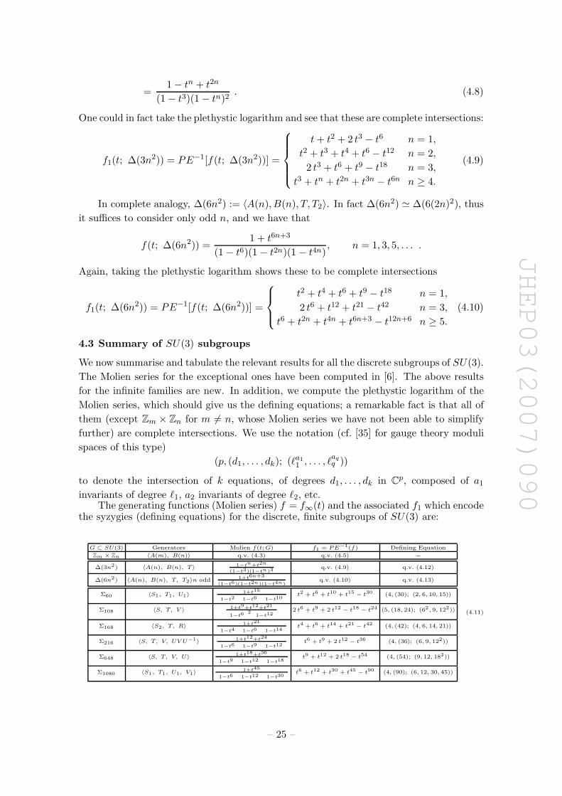
4.3 Summary of SU(3) subgroups

We now summarise and tabulate the relevant results for all the discrete subgroups of SU(3).

The Molien series for the exceptional ones have been computed in [6]. The above results

for the infinite families are new. In addition, we compute the plethystic logarithm of the

Molien series, which should give us the defining equations; a remarkable fact is that all of

them (except Zm × Zn for m 6= n, whose Molien series we have not been able to simplify

further) are complete intersections. We use the notation (cf. [35] for gauge theory moduli

spaces of this type)

(p, (d1, . . . , dk); (`a11 , . . . , `

aqq ))

to denote the intersection of k equations, of degrees d1, . . . , dk in Cp, composed of a1

invariants of degree `1, a2 invariants of degree `2, etc.The generating functions (Molien series) f = f∞(t) and the associated f1 which encode

the syzygies (defining equations) for the discrete, finite subgroups of SU(3) are:

G ⊂ SU(3) Generators Molien f(t; G) f1 = PE−1(f) Defining Equation

Zm × Zn 〈A(m), B(n)〉 q.v. (4.3) q.v. (4.5) −

∆(3n2) 〈A(n), B(n), T〉 1−tn+t2n

(1−t3)(1−tn)3q.v. (4.9) q.v. (4.12)

∆(6n2) 〈A(n), B(n), T, T2〉n odd 1+t6n+3

(1−t6)(1−t2n)(1−t4n)q.v. (4.10) q.v. (4.13)

Σ60 〈S1, T1, U1〉 1+t15ş1−t2

ť ş1−t6

ť ş1−t10

ť t2 + t6 + t10 + t15 − t30 (4, (30); (2, 6, 10, 15))

Σ108 〈S, T, V 〉 1+t9+t12+t21ş1−t6

ť 2 ş1−t12

ť 2 t6 + t9 + 2 t12 − t18 − t24 (5, (18, 24); (62, 9, 122))

Σ168 〈S2, T, R〉 1+t21ş1−t4

ť ş1−t6

ť ş1−t14

ť t4 + t6 + t14 + t21 − t42 (4, (42); (4, 6, 14, 21))

Σ216 〈S, T, V, UV U−1〉 1+t12+t24ş1−t6

ť ş1−t9

ť ş1−t12

ť t6 + t9 + 2 t12 − t36 (4, (36); (6, 9, 122))

Σ648 〈S, T, V, U〉 1+t18+t36ş1−t9

ť ş1−t12

ť ş1−t18

ť t9 + t12 + 2 t18 − t54 (4, (54); (9, 12, 182))

Σ1080 〈S1, T1, U1, V1〉 1+t45ş1−t6

ť ş1−t12

ť ş1−t30

ť t6 + t12 + t30 + t45 − t90 (4, (90); (6, 12, 30, 45))

(4.11)

– 25 –

JHEP03(2007)090

In the table, the defining equations for the Delta-series are:

∆(3n2) '

(4, (6); (1, 2, 3, 3)) n = 1,

(4, (12); (2, 3, 4, 6)) n = 2,

(4, (18); (3, 3, 6, 9)) n = 3,

(4, (6n); (3, n, 2n, 3n)) n ≥ 4.

(4.12)

and

∆(6n2)n odd '

(4, (18); (2, 4, 6, 9)) n = 1,

(4, (42); (6, 6, 12, 21)) n = 3,

(4, (12n + 6); (6, 2n, 4n, 6n + 3)) n ≥ 5.

(4.13)

The exceptional groups are addressed in [6] and our defining equations, obtained from

f1, agrees completely with Theorem C of p7 therein. The forms of the actual equations,

with the coefficients, are very complicated and the reader is referred to the aforementioned

theorem in cit. ibid.

4.4 The fundamental generating function: the Hilbert series

Before we proceed to discuss other fascinating features of C3-orbifolds in the ensuing sec-

tion, let us venture on a small digression. In many expressions above, we have seen the

power of the plethystic programme: how the plethystic logarithm of the Molien series en-

codes the geometrical information of the orbifold, with the situation even more conspicuous

for complete intersections. We advertised in the introduction and in [4], the paramountcy of

the fundamental generating function f∞ = g1, here we shall explain why it should capture

the geometry.

Let us give the formal definition of the Hilbert Series (cf. e.g. [29]). Let M :=⊕i

Mi be

a graded module over K[x1, . . . , xn] (for K some field) with respect to weights w1, . . . wn,

then the Hilbert Series is the generating function for the dimension of the graded pieces:

H(t;M) :=∑

i

dimK(Mi)ti .

Usually, we take K to be C and are working over polynomials in n variables; in this case,

the grading i can be taken to be the total degree and dimK(Mi) is simply the number of

independent polynomials at degree i. The fundamental property of the Hilbert Series is

that it is, in fact, a rational function, of the form

H(t;M) =Q(t)

n∏i=1

(1 − twi)

, (4.14)

where Q(t) is some, in general rather complicated, polynomial.

In the case of orbifolds, the Molien series counts the invariant polynomials of a given

degree. Since the syzygies (relations) of these invariants define the orbifold as a variety,

the Molien series is therefore the Hilbert series for the orbifold [6]. It just so happens that

in this case, we have a nice way to compute the Hilbert series, using the data of the finite

– 26 –

JHEP03(2007)090

group, viz., expression (3.1). In the case of toric singularities, the situation is similar, the

equivariant index of [9] and the equivalent sum over vertices in (p, q)-webs in [4], reduces

the evaluation of the Hilbert series to combinatorics of the toric diagram.

Let us illustrate the foregoing generalities. Take our familiar ∆(27) orbifold; we recall

from (4.8) that f∞(t;∆(27) = 1−t3+t6

(1−t3)3 . Now, this can in fact be re-written into what was

dubbed “Euler form” in [4], i.e.,

f∞(t;∆(27) =1 − t3 + t6

(1 − t3)3=

1 − t18

(1 − t3)2 (1 − t6) (1 − t9). (4.15)

In this form, both numerator and denominator are products of (1−twi) factors. Then, from

(4.14), geometrically, C3/∆(27) could be realised in C[x1, . . . , x4] with weights (3, 3, 6, 9).

This choice of weights arises because the 4 primitive invariants polynomials in the coordi-

nates (x, y, z) of C3 are respectively of degrees 3,3,6 and 9. Recall further, from §5.2 of [4],

that (mi, wj ≥ 0 and not necessarily distinct)

PE−1

∏i(1 − tmi)

∏j(1 − twj )

=

∑

i

tmj −∑

j

twj ,

we have from (4.15) that

f1(t;∆(27)) = PE−1[f∞(t;∆(27))] = 3 t3 + t6 + t9 − t18 ,

in agreement with (4.9). Therefore, indeed the Hilbert series has the promised properties

and indeed we see why f1 should encode the geometric information of the variety.

Two cautionary notes. Though the denominator of the Hilbert series is always in Euler

form, specifiying essentially the information about the embedding space, the numerator

Q(t) is in general complicated. When Q(t) can indeed be placed into Euler form, f1

terminates and M is a complete intersection; otherwise, f1 is an infinite series, encoding

progressively higher syzygies. Second, the form of the Hilbert series is sensitively dependent

on the choice of embedding. Had we not chosen the weights (3, 3, 6, 9) for the above

example, but, rather, have simply tried to find relations among the 4 primitive invariants,

we would have found a complete intersection whose Hilbert series is (1−t18)(1−t)4

, which would

not have given enough information about the geometry of the orbifold.

5. Discrete torsion

One might wonder what happens if one were turn on discrete torsion for the orbifold probe

theories. In the D-brane probe context, this was initiated by [30, 31]. In [32], it was

realised that the most systematic approach is to compute the so-called covering group

G of the orbifold group G. The discrete torsion then corresponds to the second group-

cohomology A = H2(G,U(1)), which is an Abelian group (so-called Schur multiplier) such

that G/A ' G.

For all subgroups of SU(2), the Schur multiplier is trivial and hence the corresponding

N = 2 gauge theories do not admit discrete torsion. For the subgroups of SU(3), however,

– 27 –

JHEP03(2007)090

the situation is more interesting and the discrete-torsion and the corresponding Schur

multipliers and covering groups have been computed and classified in [32].

The moduli space for the discrete torsion theories for Zn × Zn has been expounded in

detail in [31] (cf. also [33] for a non-commutative perspective). In general (cf. Section 3.2

of [31]), for N D3-branes, it is a U(N) theory with 3 adjoints φi=1,2,3 which are N × N

matrices, and with a superpotential

W = Tr[φ1(φ2φ3 − ω−1

n φ3φ2)]

. (5.1)

As an illustration, let us first study the simplest case of N = 1. Here, the superpotential

is W = (1 − ω−1n )φ1φ2φ3 and the gauge invariants are simply the 3 numbers φi=1,2,3. The

moduli space is therefore just the F-flat solutions, which are φ1φ2 = φ2φ3 = φ3φ1 = 0.

Hence, the moduli space M consists of 3 branches, all touching at the origin: the first

parametrized by φ1 non zero and φ2 = φ3 = 0, and the other 2 being cyclic permutations.

To construct the generating function we will use a notion called surgery [34]. It is trivial

for this case but is generically powerful for more involved cases. Since each branch of M is

the complex line we have three U(1) isometries (this holds true for higher N as well) and

g1 gets a contribution 1/(1 − ti) for each i = 1, 2, 3. We sum all together as the spaces are

not intersecting at generic points but need to subtract the intersection spaces which here is

just the one point at the origin. The result for the fundamental generating function is thus

g1 = 1/(1− t1)+1/(1− t2)+1/(1− t3)−2 Setting ti = t gives f∞(t) = g1(t) = 3/(1− t)−2.

Taking the plethystic logarithm gives us an infinite series 3t − 3t2 + 2t3 − . . ., whose first

two terms whereby agrees with the F-flat equation above.

5.1 Example: Z2 × Z2

Now, how do we reproduce the above quantities using our Hilbert series and plethystic

programme? Let us consider in detail the Z2 × Z2 example. With our discrete torsion, we

have one U(N) gauge group with three chiral fields and superpotential W = Tr(XY Z +

XZY ). Thus the F-terms induce anti-commutative relations, viz., XY = −Y X,XZ =

−ZX,Y Z = −ZY . This is the simplest example which allows discrete torsion and [31]

claims that the solution (F-terms plus D-terms) is given by

X = X1 ⊗ σ1, Y = Y1 ⊗ σ2, Z = Z1 ⊗ σ3, (5.2)

where σi are Pauli matrices and X1, Y1, Z1 all commute and so can be chosen to be all

diagonal.

To construct the single-trace gauge invariant mesonic operators, we write down the

general form as Tr(Xn1Y n2Zn3) with ni = 0, ...,∞. Because σ2i = I we can divide such

operators into eight cases

• (1) All ni are even, i.e., ni = 2ki. In this case we have the sum as

∞∑

ki=0

(t21)k1(t22)

k2(t23)k3 =

1

(1 − t21)(1 − t22)(1 − t23);

– 28 –

JHEP03(2007)090

• (2) One of the ni is odd. We will have three sub-cases. Let us focus on the case

n1 = 2k1, n2 = 2k2, n3 = 2k3 + 1. It is easy to see that Tr(σ3) = 0. Thus, this

category does not give non-zero meson operators.

• (3) One of ni is even. Again there are three sub-cases and we focus on the case where

n1 = 2k1, n2 = 2k2 + 1, n3 = 2k3 + 1. It is easy to see that Tr(σ2σ3) = 0. Thus the

contribution in this category is again zero.

• (4) The last case is that all ni are odd, n1 = 2k1 +1, n2 = 2k2 +1, n3 = 2k3 +1 Using

Tr(σ1σ2σ3) ∼ Tr(I) 6= 0, we have the counting

∞∑

ki=0

t1t2t3(t21)

k1(t22)k2(t23)

k3 =t1t2t3

(1 − t21)(1 − t22)(1 − t23).

• (5) It can be shown that Tr(X2kY 2kZ2k) = Tr((XY Z)2k), thus we need to be careful

about double-counting. However, categories (1) and (4) have different powers (even

or odd), so we do not have a double-counting problem here.

Adding the above two together we have the final counting to be,

f∞(t1, t2, t3; C3/Z

22)torsion =

1 + t1t2t3(1 − t21)(1 − t22)(1 − t23)

.

We should take the plethystic logarithm to check the equation for moduli space. It should

be the form xyz = t2. To see this let us first set t1 = t2 = t3 = t and take pletytistic

logarithm and indeed we get (terminating) polynomial expression, 3t2 + t3 − t6, which is

exactly what we should have, as one could see from case m = 2 of (4.5). Indeed, for

N = 1, it does not give a three-dimension moduli space, but, rather, a degenerate one-

dimensional one which is what was argued above from [31], viz., 3(1−t)2

. We can be more

refined and actually compute the full plethystic logarithm with all three variables, giving

us t21 + t22 + t23 + t1t2t3 − (t1t2t3)2.

5.2 The general Zn × Zn case

Let us proceed to the general case. For the group Zn × Zn, with action

g1 : (z1, z2, z3) → (z1, e− 2πi

n z2, e2πin z3), (5.3)

g2 : (z1, z2, z3) → (e2πin z1, z2, e

− 2πin z3) , (5.4)

the discrete torsion is Zn, with the 2-cocycle class given by εm((a, b), (a′, b′)) = ζm(ab′−a′b)

and ζ := eπin for n even or ζ = e

2πin for n odd. We will consider the case that gcd(m,n) = 1,

for which the projective representation is given by

γ1(g1) = P, γ1(g2) = Q , (5.5)

– 29 –

JHEP03(2007)090

with P and Q being the following n × n matrix (where ε = ζ2m and εn = 1)

P =

0 1 0 · · · 0

0 0 1 · · · 0

· · · · · · · · · · · · · · ·0 0 · · · 0 1

1 0 0 · · · 0

, Q =

0 ε 0 · · · 0

0 0 ε2 · · · 0

· · · · · · · · · · · · · · ·0 0 · · · 0 εn−1

1 0 0 · · · 0

for n odd. For n even, P is the same, while Q is (with δ2 = ε):

Q =

0 δ 0 · · · 0

0 0 δ3 · · · 0

· · · · · · · · · · · · · · ·0 0 · · · 0 δ2n−3

δ2n−1 0 0 · · · 0

.

We have the following properties

PQ = εQP, Pn = 1 = Qn, Tr(P k) = Tr(Qk) = Tr(QrQk−r) = 0, if k 6= nZ .(5.6)

Under the condition gcd(m,n) = 1, the theory has gauge group U(M), with three

chiral adjoint fields φi and superpotential Tr(φ1φ2φ3 − ε−1φ1φ3φ2). This gives F-term

condition

φiφj − ε−1φjφi, (i, j) = (1, 2), (2, 3), (3, 1) . (5.7)

Again, the solution of F-terms and D-terms relation is given by

φ1 = X ⊗ Q, φ2 = Y ⊗ P, φ3 = Z ⊗ (QP )−1 , (5.8)

where X,Y,Z all commute, just like parent N = 4 theory. Now, we consider the mesonic

operators Tr(φn11 φn2

2 φn33 ) and write ni = nki + si with ki = 0, ...,∞ and si = 0, ..., n − 1.

The key part is to see if Tr(Qs1P s2(QP )−s3) is zero (where we have used the fact that

Pn = Qn = I).

To see the properties of P,Q we use the following observation. We take P,Q as the

action of n-dimensional vector space with basis e0, ..., en−1. Then the action is as follows

(for simplicity we assume n is odd)

P (ei) = ei+1, Q(ei) = εi+1ei+1 , (5.9)

whence we have

P k(ei) = ei+k, Tr(P k) = 0, if k 6= nZ

Qk(ei) = (k∏

r=1

εi+r)(ei+k) = εki+k(k+1)

2 (ei+k), Tr(Qk) = 0, if k 6= nZ

P r1Qr2(ei) = P r1εr2i+r2(r2+1)

2 (ei+r2) = εr2i+r2(r2+1)

2 (ei+r1+r2),

– 30 –

JHEP03(2007)090

Tr(P r1Qr2) = δ(r1 + r2 − nZ)n−1∑

i=0

εr2i+r2(r2+1)

2 = εr2i+r2(r2+1)

2 δ(r1 + r2 − nZ)δ(r2 − nZ)

= εr2i+r2(r2+1)

2 δ(r1 − nZ1)δ(r2 − nZ2) .

The last equation is very important; it tells us that we need r1, r2 to be integer when

multiplying by n.

Now, we calculate

(QP )r = εr(r−1)

2 QrP r

Qs1P s2(QP )−s3 = Qs1P s2εs3(s3+1)

2 Q−s3P−s3

∼ P s2−s3Qs1−s3 .

From this we can see that Tr(Qs1P s2(QP )−s3) 6= 0 when and only when s1−s3 = nZ1, s2−s3 = nZ2. Also, because si ∈ [0, n − 1] we have the only possibility that Z1 = Z2 = 0.

With all these analysis we have following counting

f∞(t1, t2, t3; C3/Z

2n)torsion =

∞∑

ki=0

n−1∑

si=0

∑

Z1,Z2

tnk1+s11 tnk2+s2

2 tnk3+s33

×δ(s1 − s3 − nZ1)δ(s2 − s3 − nZ2)

=1

(1 − tn1 )(1 − tn2 )(1 − tn3 )

(1 − (t1t2t3)n)

(1 − t1t2t3).

First, for simplicity we can set all ti to be equal to t and get (1−t3n)(1−t3)(1−tn)3

. For n = 2 it

goes back to our previous result. Taking the plethytistic logarithm we get the (terminated)

polynomial t3 + 3tn − t3n which is the equation of xyz = tn with t degree three and x, y, z

degree n. We can also compute the full plethystic logarithm including the three variables

and obtain tn1 + tn2 + tn3 + t1t2t3 − (t1t2t3)n.

It is very interesting to notice that, comparing with (4.6) and (4.7), the result for

Zn × Zn with torsion is same as the one without discrete torsion. This is consistent with

our claim that at least for complete intersection geometries we can get the fundamental

invariant g1(t) using defining equation directly. And indeed, the defining equation does not

distinguish if there is torsion or not.

In fact, for an orbifold action, there are three parts: (1) The adjoint action on Chan-

Paton factors; (2) The space-time action on the three chiral multiples X,Y,Z; and (3) The

projected superpotential coming from Clebesh-Gordon coefficients. To get the quiver, we

need to know the information of the first two parts only. The space-time action is always a

faithful representation while the Chan-Paton action could be projective. However, because

it is an adjoint action, the cocycle factor does not affect the discussion and this is why

we can use the covering group to get the quiver diagram. The difference between faithful

representation and projective representation is that the dimension of matrix is different,

thus, given N D3-brane probes we have less number of gauge groups under projective

representation. For example, for Zn × Zn, in the minimum case we have only one gauge

– 31 –

JHEP03(2007)090

group for projective representation while for the faithful one (without discrete torsion), we

have U(1)n2

gauge groups.

To determine the theory completely, we need to know the superpotential as well;

now, the difference between projective and faithful representations gives different F-term

relations. However, as we have emphasized that the space-time action is the same with

or without discrete torsion, it is reasonable that we get the same answer and the Molien

(Hilbert) series seems to apply. Although we have not checked all cases where the geometry

may or may not be complete intersection, we do conjecture that counting will be same in

all such cases.

6. Hilbert schemes and symmetric products

We have delved into orbifolds and quotients quite intensively in the foregoing discussions.

Of key significance in our derivation in [4] for g(ν, t) is that the full generating function for

all finite N relies on an important quotient, viz., the space

SymN (M) := MN/SN , (6.1)

the N -th symmetric product of a space M. This is important because if M is the vacuum

moduli space of a single D3-brane probe (i.e., the transverse Calabi-Yau singularity), then

MN/SN is that of a stack thereof. In general, MN/SN may have singularities, however,

there is a canonical resolution called the Hilbert scheme [37], which is much richer in

structure than the mere moduli space of N (non-coinciding) points in M as captured by

MN/SN .

Formally, the Hilbert scheme is defined to be the set of all sub-schemes (we switch lib-

erally between schemes and ideals using the algebra-geometry correspondence) of a variety

X of length N , i.e.,

Hilbn(X) := {ideals I ⊂ X|dim(X/I) = N} . (6.2)

In dimension 1, everything is easy and we have that

HilbN (C) = SymN (C), HilbN (P1) = PN . (6.3)

6.1 The second symmetric product of Cm

Let us see what we can say about Cm. We know that

gN (t; M) = g1(t; SymN (M)), (6.4)

and that

g1(t; Cm) = f∞(t; C

m) =1

(1 − t)m. (6.5)

In fact, the expression is refined asm∏

i=1

1(1−ti)

. Some immediate results can be read off for

N = 2. Here, S2 ' Z2. Take m = 2, we have that

Sym2(C2) ' C[x1, y1, x2, y2]Z2 , Z2 ' 〈

(0 0 1 0

0 0 0 1

1 0 0 0

0 1 0 0

)〉 ; (6.6)

– 32 –

JHEP03(2007)090

so the Molien series and the corresponding plethystic logarithm are simply

M(t) = f∞(t) =1 + t2

(1 − t)4 (1 + t)2, f1(t) = PE−1[f(t)] = 2 t + 3 t2 − t4 . (6.7)

Again, this has a refinement and f1 = t1 + t2 + t21 + t1t2 + t22 − t21t22. This is consistent

with the fact that the defining equation for C4/Z2 with our chosen action, is a complete

intersection. It is given as a single relation (of degree 4) amongst 5 primitive (2 linear and

3 quadratic) invariants (the syzygies can be readily computed using [36]):

Y1,...,5 := {x1 + x2, y1 + y2, x12 + x2

2, x1 y1 + x2 y2, y12 + y2

2}; (6.8)

⇒ Y22 Y3 − 2Y1 Y2 Y4 + 2Y4

2 + Y12 Y5 − 2Y3 Y5 = 0 .

It is clear here that the refinement comes from an independent counting of x’s and y’s. Set

t1 to count x’s, t2 to count y’s and the equation for f1 follows.

Next, we can take m = 3 and N = 2. Now, we have that

Sym2(C3) ' C[x1, y1, z1, x2, y2, z2]Z2 , Z2 ' 〈

0 0 0 1 0 0

0 0 0 0 1 0

0 0 0 0 0 1

1 0 0 0 0 0

0 1 0 0 0 0

0 0 1 0 0 0

〉 , (6.9)

giving us

M(t) = f∞(t) =1 + 3 t2

(1 − t)6 (1 + t)3; f1(t) = 3 t+6 t2−6 t4+8 t6−18 t8+O(t10) . (6.10)

Already, here, we see from the expression for f1 that the space is not a complete intersection.

Here, the refinement is interesting:

g1 =1 + t1t2 + t2t3 + t3t1∏3

i=1(1 − ti)(1 − t2i ), (6.11)

giving

t1 + t2 + t3 +∑

i≤j

titj −∑

i<j

(titj)2 − t1t2t3(t1 + t2 + t3) + ... (6.12)

A general formula for g2 of any m is the following:

g2(t1, . . . , tm; Cm) =

(m∏

i=1

(1 − ti)(1 − t2i )

)−1

×

1 +

∑

i<j

titj +∑

i<j<k<l

titjtktl +Similar order

6 term+ . . .

As a historical digression, the series coefficients of M(t) for Sym2 of Cm are known as

Paraffin (or Alkane) Numbers, having to do with reading off diagonals of Losanitsch’s

generalisation of Pascal’s triangle [26, 27].

– 33 –

JHEP03(2007)090

6.2 The n-th symmetric product of C2

Alternatively, one could analyse the family

Symn(C2) ' C[x1, y1; x2, y2; . . . ; xn, yn]/Sn ,

where (x, y) are the coordinates of C2 and Sn permutes the n-tuple of points (xi, yi). This

is very much in the spirit of Hilbert scheme of points on surfaces as detailed in [37]. In fact,

in this case, [38] has given, in our notation, the ν-inserted plethystic exponential (cf. Eq

(4.5), cit. Ibid.):

g(ν, t1, t2; C2) = PEν [((1 − t1)(1 − t2))

−1] = exp

[ ∞∑

k=1

νk

k(1 − tk1)(1 − tk2)

]. (6.13)

Unrefining by setting t1 = t2 = t and power expanding in ν, gives, for the coefficient of νn,

the Hilbert series for Symn(C2):

PEν [1

(1 − t)2] = 1 +

1

(1 − t)2ν +

1 + t2

(1 − t)4(1 + t)2ν2 +

1 + t2 + 2 t3 + t4 + t6

(1 − t)4 (1 + t)2 (1 − t3)2ν3 + O(ν4)

(6.14)

We see that the ν-term is indeed that of Sym1(C2) = C2 and the ν2-term is what we

calculated in (6.7) for Sym2(C2).

This is, of course, in perfect congruence with our proposal in [4]: that the ν-inserted

plethystic exponential of the Hilbert series should give the generating function for gN ,

the multi-trace generating function for N D3-branes. Indeed, the coefficient to νN in

(6.14) is the Hilbert series f∞ = g1 of SymN (C2). However, recalling from (6.4) that

g1(t; SymN (C2)) = gN (t; C2), the agreement is re-assuring.

In fact, [26], the series-expansion in t for the n-th coeffcient, i.e., the t-expansion for the

Hilbert series of Symn(C2) gives the planar integer partitions (Young-Tableaux) of trace n.

That is to say, the coefficient of tm corresponds to the number of ways of writing the given

integer m as∑

i,j zi,j with zi,j ∈ Z+ such that zi+1,j > zi,j , zi,j+1 > zi,j and∑

i,i zi,i = n.

7. A detailed analysis of Y p,q

Having indulged ourselves with quotient spaces, let us change our palatte awhile to toric

varieties. The space Y p,q (cf. e.g. [7, 8, 39 – 41]) was studied in detail in [4]. The toric

data is given by the integer lattice points O = (0, 0, 1), A = (1, 0, 1), B = (0, p, 1) and

C = (−1, p − q, 1) as drawn in figure 2. As indicated, we take the trianglization of the

toric diagram by connecting the point Ta := (0, a, 1) to A and C with a = 1, ..., p (so that

Tp = B). Thus, we have 2p triangles given by TaATa+1 and TaCTa+1, a = 0, ..., p − 1.

From this we can read out the fundamental generating function f∞ (cf. [4]) as

f(x, y, z; Y p,q) =

p−1∑

a=0

1

(1 − x)(1 − xa y

za

) (1 − x−1−a z1+a

y

)

– 34 –

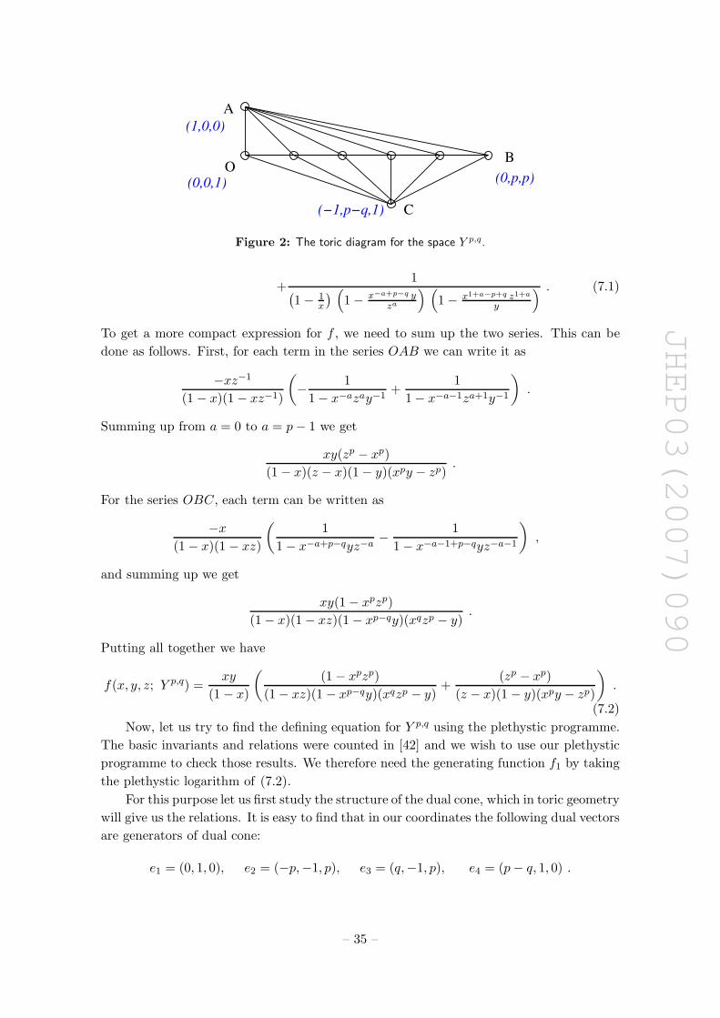
JHEP03(2007)090

(−1,p−q,1)

O

(1,0,0)

(0,0,1)

A

B

(0,p,p)

C

Figure 2: The toric diagram for the space Y p,q.

+1

(1 − 1

x

) (1 − x−a+p−q y

za

) (1 − x1+a−p+q z1+a

y

) . (7.1)

To get a more compact expression for f , we need to sum up the two series. This can be

done as follows. First, for each term in the series OAB we can write it as

−xz−1

(1 − x)(1 − xz−1)

(− 1

1 − x−azay−1+

1

1 − x−a−1za+1y−1

).

Summing up from a = 0 to a = p − 1 we get

xy(zp − xp)

(1 − x)(z − x)(1 − y)(xpy − zp).

For the series OBC, each term can be written as

−x

(1 − x)(1 − xz)

(1

1 − x−a+p−qyz−a− 1

1 − x−a−1+p−qyz−a−1

),

and summing up we get

xy(1 − xpzp)

(1 − x)(1 − xz)(1 − xp−qy)(xqzp − y).

Putting all together we have

f(x, y, z; Y p,q) =xy

(1 − x)

((1 − xpzp)

(1 − xz)(1 − xp−qy)(xqzp − y)+

(zp − xp)

(z − x)(1 − y)(xpy − zp)

).

(7.2)

Now, let us try to find the defining equation for Y p,q using the plethystic programme.

The basic invariants and relations were counted in [42] and we wish to use our plethystic

programme to check those results. We therefore need the generating function f1 by taking

the plethystic logarithm of (7.2).

For this purpose let us first study the structure of the dual cone, which in toric geometry

will give us the relations. It is easy to find that in our coordinates the following dual vectors

are generators of dual cone:

e1 = (0, 1, 0), e2 = (−p,−1, p), e3 = (q,−1, p), e4 = (p − q, 1, 0) .

– 35 –

JHEP03(2007)090

However, these are the generators of the dual cone over R+, we need the generators over

Z+. This is to say that the above four vectors are not complete in the sense of lattice

points, and there will exist some integer vectors, which are linear combinations of these

four with positive real number coefficients, but not with positive integer coefficients.

To find these missing vectors, first we notice that e3 − e2 = (p + q, 0, 0), thus the

following (p + q + 1) vectors

e23,m = e2 + (m, 0, 0) = (−p + m,−1, p), m = 0, ..., p + q

must be included into the Z+-generators of the dual cone. Similarly, since e4 − e1 =

(p − q, 0, 0), the following (p − q + 1) vectors should also be included:

e14,m = (m, 1, 0), m = 0, ..., p − q .

We are not finished yet. From the fact that e3 + e4 = (p, 0, p) we find that we need (1, 0, 1)

and from e1 + e2 = (−p, 0, p), we need (−1, 0, 1). Finally, from these two we get (0, 0, 2) so

we need (0, 0, 1) as generator. Thus we have three more generators

e5 = (1, 0, 1), e6 = (−1, 0, 1), e7 = (0, 0, 1) .

Putting all together we have 2p + 5 generators e23,m, e14,m, e5, e6, e7 as claimed by [42].

To have a simple result for the plethystic logarithm, we want as many as generators

having same degree. One simple choice could be the following scaling: x → 1, y → tp, z → t2

under which the generators e23,m and e14,m have same degree. However, when p is even,

there is an interference between the number of variables and the number of equations

for the definition of geometry. By this we mean that in expanding the expression for the

plethystic logarithm, positive terms signify invariants while negative terms signify relations,

these could potentially cancel and confuse the counting; this situation was encountered in

the example of the non-complete intersection C3/Z3 in [4]. Thus the above scaling is not

a good choice. Another choice will be the x → 1, y → t2p−1, z → t4. In this case, e23,m and

e14,m do not have same degree, but the interference is avoided.

However, we can do better by having multiple variables in the plethystic logarithm.

To do so, first we need to set x → 1. The reason is very simple because we want to set

e23,m (as well as e14,m) to have the same degree. After this we have

f(x → 1, y, z; Y p,q) =yA + y2B + y3C

(1 − y)2(1 − z)2(y − zp)2;

A := −zp(zp+1(p − q − 1) − zp(p − q + 1) + z(p + q + 1) − (p + q − 1))

B := (1 + z)(1 − z2p) − 4pzp(1 − z)

C := −zp+1(p + q − 1) + zp(p + q + 1) − z(p − q + 1) + (p − q − 1) .

In this form, it is not suitable to take the plethystic logarithm because of the overall factor

y in the numerator as well as the factor (y − zp) in the denominator, which would give

a logarithmic singularity in at y = 0. To amend this, we change variables as y → y and

z → ty. Thus

f(x → 1, y, ty; Y p,q) =A + B + yC

(1 − y)2(1 − ty)2(1 − tpyp−1)2

– 36 –

JHEP03(2007)090

A := −tpyp−1((ty)p+1(p − q − 1) − (ty)p(p − q + 1) + ty(p + q + 1) − (p + q − 1))

B := (1 + ty)(1 − (ty)2p) − 4p(ty)p(1 − ty)

C := −(ty)p+1(p + q − 1) + (ty)p(p + q + 1) − ty(p − q + 1) + (p − q − 1) .

Now, we can take the plethystic logarithm and get the right answer! It is easy to see that

under the above scaling we have (p+q+1) variables with scaling e23,m → yp−1tp, (p−q+1)

variables with scaling e14,m → y and three variables with scaling e5,6,7 → yt.

Let us check the above result with the tabulation of the following several examples:

(p, q) f1(t, y;Y p,q)

(p = 1, q = 0) (2t + 2y) − ty

(p = 1, q = 1) (3t + y) − t2

(p = 2, q = 0) (3t2y + 3y + 3ty) − y2 − 4ty2 − 10t2y2 − 4t3y2 − t4y2 + ...

(p = 2, q = 1) (4t2y + 2y + 3ty) − 2ty2 − 9t2y2 − 6t3y2 − 3t4y2 + ...

(p = 2, q = 2) (5t2y + y + 3ty) − 6t2y2 − 8t3y2 − 6t4y2 + ...

(p = 3, q = 0) (4t3y2 + 4y + 3ty) − 3y2 − 6ty2 − t2y2 − 16t3y3 − 6t4y3 − 3t6y4 + ...

(p = 3, q = 1) (5t3y2 + 3y + 3ty) − y2 − 4ty2 − t2y2 − 15t3y3 − 8t4y3 − 6t6y4 + ...

(p = 3, q = 2) (6t3y2 + 2y + 3ty) − 2ty2 − t2y2 − 12t3y3 − 10t4y3 − 10t6y4 + ...

(p = 3, q = 3) (7t3y2 + y + 3ty) − t2y2 − 7t3y3 − 12t4y3 − 15t6y4 + ...

The interpretation of f1 was outlined in [4]. For p = 2, q = 0, for example, we should

have 3 variables with scaling t2y, 3 variables with scaling y and another 3 with scaling

ty; this is given exactly inside the first bracket. The remaining part is the information

about relations, i.e, defining equations. The term −y2 means there is one relation among

3 variables with scaling y. Similarly the term −4ty2 tells us that there are four relations

between variables with scaling y and variables with scaling yt.

Checking all examples we find that the total number of defining equations is given by

p2 +10p−4. It is different from the claim given by [42] where it is claimed that the number

of equations should be p2 + 10p − q2 − 4. However, in cit. ibid., only minimum relations

are counted. In other words, if a = b and b = c then a = c will not be counted as a new

relation. However, in our case, a = c would be counted separately.

8. Conclusions and prospects

We have proposed a plethystic programme for the counting of gauge invariant operators

in gauge theories. Though we have restricted our attention to chiral BPS mesonic operators

in world-volume theories of D-branes probing Calabi-Yau singularities, the programme

should be of wider applicability. In the case of our present focus, an intimate web of

connexions between geometry, gauge theory and combinatorics emerges. This field of quiver

theories is where the plethystics fully blossom. In a way, this does not surprise us. Indeed,

for D-brane quiver theories, the mesonic gauge invariants in the chiral ring, modulo the

F-term constraints, should give a classical moduli space that by construction is the Calabi-

Yau variety which the brane probes.

– 37 –

JHEP03(2007)090

What is beautiful about the plethystic programme is that the plethystic exponential

function and its inverse provide the explicit link between the geometry and the gauge

invariants. One only needs to construct a fundamental invariant of the Calabi-Yau manifold

M, which we have called f = f∞ = g1 and which mathematically corresponds to the

Hilbert series. This is the generating function for the single-trace operators. The plethystic

logarithm, PE−1, gives all the syzygies of M. In the case of M being complete intersection,

f1 = PE−1[f ] is a polynomial from which one immediately reads out the defining equation

of M. On the other hand, the plethystic exponential gives g∞ = PE[f ], the generating

function for the multi-trace operators.

Continuing with [4], we have provided a host of examples to demonstrate the power

of the plethystic programme, ranging from orbifold theories to toric singularities, from

discrete torsion to Hilbert schemes, touching upon such interesting curios as relations to

Young Tableaux and to the MacMahon Conjecture. Importantly, we have also, using

results of Temperley and Haselgrove, generalised the formulae of Hardy-Ramanujan and

Meinardus, in estimating the asymptotic behaviour of the number of such operators. This

is an estimate of the degrees of freedom of the gauge theory, whereby providing us with

explicit expressions for the entropy for an arbitrary number N of D-branes.

We have, of course, only touched upon the fringe of a fertile ground. How do plethystics

teach us about other branches of the moduli space? For example, it will be interesting to

count baryonic branch and to see if syzygies of divisors wrapped by D3-branes be captured

by plethystics. Including of baryonic operators into the counting should correspond to the

geometry of cycles in the Sasaki-Einstein manifold, can the syzygies of these divisors be

captured by plethystics? Recently, progress in counting baryonic operators has been made

in [22]. Along similar lines is the mixed branch studied in [34]. Can our programme be

extended to study such other branches? What about 1/4 or 1/8 BPS states?

Moreover, in [4], we have performed the counting for geometries whose quiver theories

have not yet been constructed; we could also do so for non-quiver and even non-SUSY

theories. Indeed, there has also been much study of certain indices of superconformal

theories [47 – 52] as well as the counting of instantons such as in [53]. How does our

plethystic programme relate to these counting problems? The portals to a Grecian mansion

have been opened to us, to fully explore the plethora of her plethystic secrets shall be our

continued goal.

Acknowledgments

We heartily acknowledge Nemani Suryanarayana and Balazs Szendroi for wonderful com-

munications. B.F. is obliged to the Marie Curie Research Training Network under contract

number MRTN-CT-2004-005104 and once more extends his thanks to Merton College,

Oxford for warm reception at the final stages of the draft. A.H. is grateful to Sergio

Benvenuti, Kazutoshi Ohta, Toshio Nakatsu, Yui Noma, and Christian Romelsberger for

enlightening discussions. Y.H.H. kisses the grounds of Merton College, Oxford, to whose

gracious patronage, through the FitzJames Fellowship, he owes his inspiration, and he

– 38 –

JHEP03(2007)090

kisses the hands of Senyorita L. Figuerola-Sole, whose eyes, like rays of Mediterranean sun,

pierces the scholastic melancholy of his soul.

References

[1] J.M. Maldacena, The large-N limit of superconformal field theories and supergravity, Adv.

Theor. Math. Phys. 2 (1998) 231 [hep-th/9711200].

[2] M.R. Douglas and G.W. Moore, D-branes, quivers and ALE instantons, hep-th/9603167.

[3] Y.-H. He, Lectures on D-branes, gauge theories and Calabi-Yau singularities,

hep-th/0408142; On algebraic singularities, finite graphs and D-brane gauge theories: a

string theoretic perspective, hep-th/0209230.

[4] S. Benvenuti, B. Feng, A. Hanany and Y.-H. He, Counting BPS operators in gauge theories:

quivers, syzygies and plethystics, hep-th/0608050.

[5] P. Pouliot, Molien function for duality, JHEP 01 (1999) 021 [hep-th/9812015].

[6] Stephen S.T. Yau and Y. Yu, Gorenstein quotient singularities in dimension three, Memoirs

of the AMS, no. 505, Providence, 1993.

[7] J.P. Gauntlett, D. Martelli, J. Sparks and D. Waldram, Supersymmetric AdS5 solutions of

M-theory, Class. and Quant. Grav. 21 (2004) 4335 [hep-th/0402153].

[8] J.P. Gauntlett, D. Martelli, J. Sparks and D. Waldram, Sasaki-einstein metrics on S2 × S3,

Adv. Theor. Math. Phys. 8 (2004) 711 [hep-th/0403002].

[9] D. Martelli, J. Sparks and S.-T. Yau, Sasaki-einstein manifolds and volume minimisation,

hep-th/0603021.

[10] J.P. Serre, A course in arithmetic, GTM, Springer, 1996.

[11] Y. Noma, T. Nakatsu and T. Tamakoshi, Plethystics and instantons on ALE spaces,

hep-th/0611324.

[12] G. Meinardus, Asymptotische Aussagen uber Partitionen, Mathematische Zeitschrift 59

(1954) 388.

[13] C.B. Haselgrove and H.N.V. Temperley, Asymptotic formulae in the theory of partitions,

Proc. Cambridge Phil. Soc. 50 (1954) 225.

[14] L. B. Richmond, Some general problems on the number of parts in partitions, Acta

Arithmetica, LXVI.4 (1994) p. 297.

[15] H. Hwang, Distributions of integer partitions with large number of summands, Acta

Arithmetica, 78 (1997) 351.

[16] A.A. Actor, Infinite products, partition functions, and the Meinardus theorem,

J. Mathematical Physics, Vol 35, 11, Nov. 1994, p. 5749.

[17] F.C. Auluck, S. Chowla, and H. Gupta, J. Ind. Math. Soc. 6 (1942) 105.

[18] S. Grossmann and M. Holthaus, Microcanonical fluctuations of a Bose systems ground state

occupation number, Phys. Rev. E 54 (1996) 3495.

[19] M. Gajda and K. Rzazewski, Fluctuations of Bose-Einstein condensate, Phys. Rev. Letters

78 (1997) no.14.

– 39 –

JHEP03(2007)090

[20] D. Martelli and J. Sparks, Dual giant gravitons in Sasaki-Einstein backgrounds, Nucl. Phys.

B 759 (2006) 292 [hep-th/0608060].

[21] A. Butti, D. Forcella and A. Zaffaroni, Deformations of conformal theories and non-toric

quiver gauge theories, JHEP 02 (2007) 081 [hep-th/0607147].

[22] A. Butti, D. Forcella and A. Zaffaroni, Counting BPS baryonic operators in CFTS with

Sasaki-Einstein duals, hep-th/0611229.

[23] A. Hanany and Y.-H. He, Non-abelian finite gauge theories, JHEP 02 (1999) 013

[hep-th/9811183].

[24] P. Cameron, T. Prellberg, D. Stark, Asymptotics for incidence matrix classes,

math.CO/0510155.

[25] P.A. MacMahon, Memoir on the Theory of the Partitions of Numbers. V: Partitions in

Two-Dimensional Space, Phil. Trans. Roy. Soc. London Ser. A 211, 75-110, 1912a; Memoir

on the Theory of the Partitions of Numbers, VI. Partitions in Two-Dimensional Space, to

which is Added an Adumbration of the Theory of Partitions in Three-Dimensional Space,

Phil. Trans. Roy. Soc. London Ser. A 211, 345-373, 1912b.

[26] N. Sloane, The On-Line Encyclopedia of Integer Sequences,

http://www.research.att.com/∼njas/sequences/index.html.

[27] S. M. Losanitsch, Die Isomerie-Arten bei den Homologen der Paraffin-Reihe, Chem. Ber. 30

(1897) 1917.

[28] The GAP Group, GAP – Groups, Algorithms, and Programming, Version 4.4 2006,

http://www.gap-system.org.

[29] D. Eisenbud, Commutative Algebra With A View Toward Algebraic Geometry, GTM 150,

Springer-Verlag, 1995.

[30] M.R. Douglas, D-branes and discrete torsion, hep-th/9807235.

[31] M.R. Douglas and B. Fiol, D-branes and discrete torsion, II, JHEP 09 (2005) 053

[hep-th/9903031].

[32] B. Feng, A. Hanany, Y.-H. He and N. Prezas, Discrete torsion, non-abelian orbifolds and the

schur multiplier, JHEP 01 (2001) 033 [hep-th/0010023]; Discrete torsion, covering groups

and quiver diagrams, JHEP 04 (2001) 037 [hep-th/0011192].

[33] D. Berenstein, V. Jejjala and R.G. Leigh, Marginal and relevant deformations of N = 4 field

theories and non-commutative moduli spaces of vacua, Nucl. Phys. B 589 (2000) 196

[hep-th/0005087].

[34] A. Hanany and C. Romelsberger, Counting BPS operators in the chiral ring of N = 2

supersymmetric gauge theories or N = 2 braine surgery, hep-th/0611346.

[35] J. Gray, Y.-H. He, V. Jejjala and B.D. Nelson, Exploring the vacuum geometry of N = 1

gauge theories, Nucl. Phys. B 750 (2006) 1 [hep-th/0604208]; The geometry of particle

physics, Phys. Lett. B 638 (2006) 253 [hep-th/0511062].

[36] D. Grayson and M. Stillman, Macaulay 2, a software system for research in algebraic

geometry, available at http://www.math.uiuc.edu/Macaulay2/.

[37] Hiraku Nakajima, Lectures on Hilbert schemes of points on surfaces, American Mathematical

Society, Providence, RI, 1999.

– 40 –

JHEP03(2007)090

[38] Hiraku Nakajima, Kota Yoshioka, Instanton counting on blowup, I. 4-dimensional pure gauge

theory, math.AG/0306198.

[39] D. Martelli and J. Sparks, Toric geometry, sasaki-einstein manifolds and a new infinite class

of AdS/CFT duals, Commun. Math. Phys. 262 (2006) 51 [hep-th/0411238].

[40] S. Benvenuti, S. Franco, A. Hanany, D. Martelli and J. Sparks, An infinite family of

superconformal quiver gauge theories with Sasaki-Einstein duals, JHEP 06 (2005) 064

[hep-th/0411264].

[41] S. Benvenuti, A. Hanany and P. Kazakopoulos, The toric phases of the y(p,q) quivers, JHEP

07 (2005) 021 [hep-th/0412279]; Conformal manifolds for the conifold and other toric field

theories, JHEP 08 (2005) 024 [hep-th/0502043];

A. Hanany, P. Kazakopoulos and B. Wecht, A new infinite class of quiver gauge theories,

JHEP 08 (2005) 054 [hep-th/0503177];

H. Kihara, M. Sakaguchi and Y. Yasui, Scalar laplacian on Sasaki-Einstein manifolds y(p,q),

Phys. Lett. B 621 (2005) 288 [hep-th/0505259].

[42] S. Pinansky, Quantum deformations from toric geometry, JHEP 03 (2006) 055

[hep-th/0511027].

[43] S. Lee, Superconformal field theories from crystal lattices, hep-th/0610204.

[44] T. Oota and Y. Yasui, New example of infinite family of quiver gauge theories, Nucl. Phys. B

762 (2007) 377 [hep-th/0610092].

[45] A. Sinha, J. Sonner and N.V. Suryanarayana, At the horizon of a supersymmetric AdS5 black

hole: isometries and half-BPS giants, JHEP 01 (2007) 087 [hep-th/0610002].

[46] A. Basu and G. Mandal, Dual giant gravitons in AdS(m) × yn (Sasaki-Einstein),

hep-th/0608093.

[47] J. Kinney, J.M. Maldacena, S. Minwalla and S. Raju, An index for 4 dimensional super

conformal theories, hep-th/0510251.

[48] C. Romelsberger, Counting chiral primaries in N = 1, D = 4 superconformal field theories,

Nucl. Phys. B 747 (2006) 329 [hep-th/0510060].

[49] I. Biswas, D. Gaiotto, S. Lahiri and S. Minwalla, Supersymmetric states of N = 4 Yang-Mills

from giant gravitons, hep-th/0606087.

[50] G. Mandal and N.V. Suryanarayana, Counting 1/8-BPS dual-giants, hep-th/0606088.

[51] A. Sinha and N.V. Suryanarayana, Two-charge small black hole entropy: string-loops and

multi-strings, JHEP 10 (2006) 034 [hep-th/0606218].

[52] Y. Nakayama, Index for orbifold quiver gauge theories, Phys. Lett. B 636 (2006) 132

[hep-th/0512280]; Index for supergravity on AdS5 × T (1,1) and conifold gauge theory, Nucl.

Phys. B 755 (2006) 295 [hep-th/0602284].

[53] F. Fucito, J.F. Morales and R. Poghossian, Instanton on toric singularities and black hole

countings, JHEP 12 (2006) 073 [hep-th/0610154].

– 41 –