Invariants of Combinatorial Line Arrangements and Rybnikov's Example
27
arXiv:math/0403543v1 [math.AG] 31 Mar 2004 INVARIANTS OF COMBINATORIAL LINE ARRANGEMENTS AND RYBNIKOV’S EXAMPLE ENRIQUE ARTAL BARTOLO, JORGE CARMONA RUBER, JOS ´ E IGNACIO COGOLLUDO AGUST ´ IN, AND MIGUEL ´ ANGEL MARCO BUZUN ´ ARIZ Abstract. Following the general strategy proposed by G.Rybnikov, we present a proof of his well-known result, that is, the existence of two arrangements of lines having the same combinatorial type, but non-isomorphic fundamental groups. To do so, the Alexander Invariant and certain invariants of combinato- rial line arrangements are presented and developed for combinatorics with only double and triple points. This is part of a more general project to better under- stand the relationship between topology and combinatorics of line arrangements. One of the main subjects in the theory of hyperplane arrangements is the rela- tionship between combinatorics and topological properties. To be precise, one has to make the following distinction: for a given hyperplane arrangement H⊂ P n , one can study the topological type of the pair (P n , H) or the topological type of the complement P n \H. For the first concept we will use the term relative topology of H, whereas for the second one we will simply say topology of H. It is clear that if two hyperplane arrangements have the same relative topology, then they have the same topology, but the converse is not known. In a well-known and very cited work [5], G. Rybnikov found an example of two line arrangements L 1 and L 2 in the complex projective plane P 2 having the same combinatorics but different topology. The most common way to prove that two topologies of line arrangements are different is to check that the fundamental groups of their complements are not isomorphic. Recently, the authors of this work have provided an example of two line arrange- ments with different relative topologies (see [2]). The contribution of [2] is that it refers to real arrangements, that is, arrangements that admit real equations for each line (note that Rybnikov’s example cannot have real equations). The proof proposed by Rybnikov has two steps. Let G i := π 1 (P 2 \ L i ), i =1, 2. (R1) Recall that the homology of the complement of a hyperplane arrangement depends only on combinatorics. This way, one can identify the abelianization Second author is partially supported by BFM2001-1488-C02-01; others authors are partially supported by BFM2001-1488-C02-02. 1
-
Upload
fundacionuniversitarialoslibertadores -
Category
Documents
-
view
4 -
download
0
Transcript of Invariants of Combinatorial Line Arrangements and Rybnikov's Example

arX
iv:m
ath/
0403
543v
1 [
mat
h.A
G]
31
Mar
200
4
INVARIANTS OF COMBINATORIAL LINE ARRANGEMENTS
AND RYBNIKOV’S EXAMPLE
ENRIQUE ARTAL BARTOLO, JORGE CARMONA RUBER, JOSE IGNACIO
COGOLLUDO AGUSTIN, AND MIGUEL ANGEL MARCO BUZUNARIZ
Abstract. Following the general strategy proposed by G.Rybnikov, we present
a proof of his well-known result, that is, the existence of two arrangements
of lines having the same combinatorial type, but non-isomorphic fundamental
groups. To do so, the Alexander Invariant and certain invariants of combinato-
rial line arrangements are presented and developed for combinatorics with only
double and triple points. This is part of a more general project to better under-
stand the relationship between topology and combinatorics of line arrangements.
One of the main subjects in the theory of hyperplane arrangements is the rela-
tionship between combinatorics and topological properties. To be precise, one has
to make the following distinction: for a given hyperplane arrangement H ⊂ Pn,
one can study the topological type of the pair (Pn,H) or the topological type of
the complement Pn \H. For the first concept we will use the term relative topology
of H, whereas for the second one we will simply say topology of H. It is clear that
if two hyperplane arrangements have the same relative topology, then they have
the same topology, but the converse is not known.
In a well-known and very cited work [5], G. Rybnikov found an example of
two line arrangements L1 and L2 in the complex projective plane P2 having the
same combinatorics but different topology. The most common way to prove that
two topologies of line arrangements are different is to check that the fundamental
groups of their complements are not isomorphic.
Recently, the authors of this work have provided an example of two line arrange-
ments with different relative topologies (see [2]). The contribution of [2] is that
it refers to real arrangements, that is, arrangements that admit real equations for
each line (note that Rybnikov’s example cannot have real equations).
The proof proposed by Rybnikov has two steps. Let Gi := π1(P2\
⋃Li), i = 1, 2.
(R1) Recall that the homology of the complement of a hyperplane arrangement
depends only on combinatorics. This way, one can identify the abelianization
Second author is partially supported by BFM2001-1488-C02-01; others authors are partially
supported by BFM2001-1488-C02-02.1

2 E. ARTAL, J. CARMONA, J.I. COGOLLUDO, AND M.A. MARCO
of G1 and G2 with an Abelian group H combinatorially determined. Ryb-
nikov proves that no isomorphisms exist between G1 and G2 that induce the
identity on H . In particular, this result proves that both arrangements have
different relative topologies. The reason can be outlined as follows: any auto-
morphism of the combinatorics of Rybnikov’s arrangement can be obtained
from a diffeomorphism of P2, and hence it produces an automorphism of
fundamental groups. Since any homeomorphism of pairs (P2,⋃Li) induces
an automorphism of the combinatorics of⋃Li, after composition one can
assume that any homeomorphism of pairs induces the identity on H .
The strategy rests on the study of the Lower Central Series (LCS). Since
L1 and L2 are constructed using the MacLane arrangement Lω (see Exam-
ple 1.7), it is enough to study, by some combinatorial arguments, the LCS
of Lω with an extra structure (referred to as an ordered arrangement). Al-
though this part is explained in [5, Section 3], computations are hard to
verify.
(R2) The second step is essentially combinatorial. The main point is to truncate
the LCS of Gi such that the quotient K depends only on the combinatorics.
Rybnikov proposes to prove that an automorphism of K induces the identity
on H (up to sign and automorphisms of the combinatorics). This proof is
only outlined in [5, Proposition 4.2]. It is worth pointing out that such a
result cannot be expected for any arrangement. Also [5, Proposition 4.3]
needs some explanation of its own. The main difference between relative
topology and topology of the complement in terms of isomorphisms of the
fundamental group is that homeomorphisms of pairs induce isomorphisms
that send meridians to meridians, whereas homeomorphisms of the comple-
ment can induce any kind of isomorphism, and even if we know that the
isomorphism induces the identity on homology, this is not enough to claim
that meridians are sent to meridians.
The aim of our work is to follow the idea behind Rybnikov’s work and, using
slightly different techniques, provide detailed proofs of his result. This is part
of a more general project by the authors that aims to better understand the
relationship between topology and combinatorics of line arrangements.
The following is a more detailed description of the layout of this paper. In sec-
tion 1, the more relevant definitions are set, as well as a description of Rybnikov’s
and MacLane’s combinatorics. Sections 2 and 3 provide a proof of Step (R1). In
order to do so, we propose a new approach related to Derived Series, which is also
useful in the study of Characteristic Varieties and the Alexander Invariant. The

COMBINATORIAL LINE ARRANGEMENTS 3
Alexander Invariant of a group G, with a fixed isomorphism G/G′ ≈ Zr, is the
quotient G′/G′′ considered as a module over the ring Λ := Z[t±11 , . . . , t±1
r ], which
is the group algebra of Zr. By fixing an ideal m ⊂ Λ, the truncated module by
Λ/mj is studied. The problem is reduced to solving a system of linear equations.
Section 4 is devoted to the study of combinatorial properties of a line arrange-
ment which ensure that any automorphism of the fundamental group of the com-
plement essentially induces the identity on homology (that is, the analogous of [5,
Proposition 4.2]). This is an interesting question that can be applied to general
line arrangements. For the sake of simplicity, we only present our progress on line
arrangements with double and triple points. This provides a proof for the second
step (R2).
Acknowledgments
We want to thank G.Rybnikov for his contribution and his support. His work
has been a challenge for us for years.
1. Settings and Definitions
In this section, some standard facts about line combinatorics and ordered line
combinatorics will be described. Special attention will be given to MacLane and
Rybnikov’s line combinatorics.
Definition 1.1. A combinatorial type (or simply a (line) combinatorics) is a
couple C := (L,P), where L is a finite set and P ⊂ P(L), satisfying that:
(1) For all P ∈ P, #P ≥ 2;
(2) For any ℓ1, ℓ2 ∈ L, ℓ1 6= ℓ2, ∃!P ∈ P such that ℓ1, ℓ2 ∈ P .
An ordered combinatorial type C ord is a combinatorial type where L is an ordered
set.
Notation 1.2. Given a combinatorial type C , the multiplicity mP of P ∈ P is the
number of elements L ∈ L such that P ∈ L; note that mP ≥ 2. The multiplicity
of a combinatorial type is the number 1 − #L +∑
P∈P(mP − 1).
Example 1.3 (MacLane’s combinatorics). Let us consider the 2-dimensional vec-
tor space on the field F3 of three elements. Such a plane contains 9 points and 12
lines, 4 of which pass through the origin. Consider L = F23\{(0, 0)} and P, the set
of lines in F23 (as a subset of P(L)). This provides a combinatorial type structure
CML that we will refer to as MacLane’s combinatorial type. Figure 1 represents
an ordered MacLane’s combinatorial type.

4 E. ARTAL, J. CARMONA, J.I. COGOLLUDO, AND M.A. MARCO
Definition 1.4. Let C := (L,P) be a combinatorial type. We say a complex line
arrangement H := ℓ0∪ ℓ1∪ ...∪ ℓr ⊂ P2 is a realization of C if and only if there are
bijections ψ1 : L → {ℓ0, ℓ1, ..., ℓr} and ψ2 : P → Sing(H) such that ∀ℓ ∈ H, P ∈ P,
one has P ∈ ℓ⇔ ψ1(ℓ) ∈ ψ2(P ). If C ord is an ordered combinatorial type and the
irreducible components of H are also ordered, we say H is an ordered realization
if ψ1 respects orders.
Notation 1.5. The space of all complex realizations of a line combinatorics C is
denoted by Σ(C ). This is a quasiprojective subvariety of Pr(r+3)
2 , where r := #C .
If C ord is ordered, we denote by Σord(C ) ⊂ (P2)r the space of all ordered complex
realizations of C ord.
There is a natural action of PGL(3; C ) on such spaces. This justifies the fol-
lowing definition.
Definition 1.6. The moduli space of a combinatorics C is the quotient M (C ) :=
Σ(C )/PGL(3; C ). The ordered moduli space M ord(C ) of an ordered combina-
torics C ord is defined accordingly.
Example 1.7. Let us consider the MacLane line combinatorics CML. It is well
known that such combinatorics has no real realization and that #M (CML) = 1,
however #M ord(CML) = 2. The following are representatives for M ord(CML):
(1)ℓ0 = {x = 0} ℓ1 = {y = 0} ℓ2 = {x = y} ℓ3 = {z = 0} ℓ4 = {x = z}
ℓ±5 = {z + ωy = 0} ℓ±6 = {z + ωy = (ω + 1)x} ℓ±7 = {(ω + 1)y + z = x}
where ω = e2πi/3.
We will refer to such ordered realizations as
Lω := {ℓ0, ℓ1, ℓ2, ℓ3, ℓ4, ℓ+5 , ℓ
+6 , ℓ
+7 }
and
Lω := {ℓ0, ℓ1, ℓ2, ℓ3, ℓ4, ℓ−5 , ℓ
−6 , ℓ
−7 }.
4
5
1
0
2
7
6
3
Figure 1. Ordered MacLane lines in F23

COMBINATORIAL LINE ARRANGEMENTS 5
Remark 1.8. Given a line combinatorics C = (L,P), the automorphism group
Aut(C ) is the subgroup of the permutation group of L preserving P. Let us con-
sider an ordered line combinatorics C ord. It is easily seen that Aut(C ord) acts on
both Σord(C ord) and M ord(C ord). Note also that M (C ord) ∼= M ord(C ord)/Aut(C ord).
Example 1.9. The action of Aut(CML) ∼= PGL(2,F3) on the moduli spaces is
as follows: matrices of determinant +1 (resp. −1) fix (resp. exchange) the two
elements of M ord(CML). Of course complex conjugation also acts on M ord(CML)
exchanging the two elements. From the topological point of view one has that:
• There exists a homeomorphism (P2,⋃Lω) → (P2,
⋃Lω) preserving orien-
tations on both P2 and the lines. Such a homeomorphism does not respect
the ordering.
• There exists a homeomorphism (P2,⋃Lω) → (P2,
⋃Lω) preserving orien-
tations on P2, but not on the lines. Such a homeomorphism respects the
ordering.
Also note that the subgroup of automorphisms that preserve the set L0 :=
{ℓ0, ℓ1, ℓ2} is isomorphic to Σ3, since the vectors (1, 0), (1, 1) and (1, 2) generate
F23. We will denote by L+ and L− the sets of 5 lines such that Lω = L0 ∪ L+ and
Lω = L0 ∪L−. Since any transposition of {0, 1, 2} in CML produces a determinant
−1 matrix in PGL(2,F3), one concludes from the previous paragraph that any
transposition of {0, 1, 2} induces a homeomorphism (P2,⋃Lω) → (P2,
⋃Lω) that
exchanges Lω and Lω as representatives of elements of M ord(CML) and globally
fixes L0.
Example 1.10 (Rybnikov’s combinatorics). Let Lω and Lω be ordered MacLane
realizations as above, where L0 := {ℓ0, ℓ1, ℓ2}. Let us consider a projective trans-
formation ρω (resp. ρω) fixing the initial ordered set L0 (that is, ρ(ℓi) = ℓi
i = 0, 1, 2) and such that ρωLω (resp. ρωLω) and Lω intersect each other only
in double points outside the three common lines. Note that ρω, ρω can be chosen
with real coefficients.
Let us consider the following ordered arrangements of thirteen lines: Rα,β =
Lα ∪ ργLβ, where α, β ∈ {ω, ω} and γ = β (resp β) if α = ω (resp. ω). They

6 E. ARTAL, J. CARMONA, J.I. COGOLLUDO, AND M.A. MARCO
produce the following combinatorics CRyb := (R,P) given by:
(2)R := {ℓ0, ℓ1, ℓ2, ℓ3, ℓ4, ℓ5, ℓ6, ℓ7, ℓ8, ℓ9, ℓ10, ℓ11, ℓ12}
P2 :=
{ℓ2, ℓ3}, {ℓ0, ℓ7}, {ℓ1, ℓ6}, {ℓ4, ℓ5},
{ℓ2, ℓ8}, {ℓ0, ℓ12}, {ℓ1, ℓ11}, {ℓ9, ℓ10},
{ℓi, ℓj} 3 ≤ i ≤ 7, 8 ≤ j ≤ 12
P3 :=
{ℓ0, ℓ1, ℓ2}, {ℓ3, ℓ6, ℓ7}, {ℓ0, ℓ5, ℓ6}, {ℓ1, ℓ4, ℓ7}, {ℓ1, ℓ3, ℓ5},
{ℓ2, ℓ4, ℓ6}, {ℓ2, ℓ5, ℓ7}, {ℓ0, ℓ3, ℓ4}, {ℓ8, ℓ11, ℓ12} {ℓ0, ℓ10, ℓ11},
{ℓ1, ℓ9, ℓ12}, {ℓ1, ℓ8, ℓ10}, {ℓ2, ℓ9, ℓ11}, {ℓ2, ℓ10, ℓ12}, {ℓ0, ℓ8, ℓ9}
P := P2 ∪ P3
Proposition 1.11. The following combinatorial properties hold:
(1) The different arrangements Rα,β have the same combinatorial type CRyb.
(2) The set of lines L0 has the following distinctive combinatorial property: every
line in L0 contains exactly 5 triple points of the arrangement; the remaining
lines only contain 3 triple points.
(3) For the other 10 lines we consider the equivalence relation generated by the
relation of sharing a triple point. There are two equivalence classes which
correspond to Lε and ρLε′, ε, ε′ = ±.
By the previous remarks one can group the set R together in three subsets.
One is associated with the set of lines L0 (referred to as R0), and the other two
are combinatorially indistinguishable sets (R1 and R2) such that R0 ∪ R1 and
R0 ∪ R2 are MacLane’s combinatorial types. Note that any automorphism of
CRyb must preserve R0 and either preserve or exchange R1 and R2. Therefore,
Aut(CRyb) ∼= Σ3 ×Z/2Z. The following results are immediate consequences of the
aforementioned remarks.
Proposition 1.12. The following are (or induce) homeomorphisms between the
pairs (P2,⋃Rω,ω) and (P2,
⋃Rω,ω) (resp. (P2,
⋃Rω,ω) and (P2,
⋃Rω,ω)) preserv-
ing the orientation of P2:
(a) Complex conjugation, which reverses orientations of the lines.
(b) A transposition in R0, which preserves orientations of the lines.
We will refer to Rω,ω and Rω,ω (resp. Rω,ω and Rω,ω) as a type + (resp. type −)
arrangements.
Proposition 1.13. Any homeomorphism of pairs between a type + and a type −
arrangement should lead (maybe after composing with complex conjugation) to an

COMBINATORIAL LINE ARRANGEMENTS 7
orientation-preserving homeomorphism of pairs between a type + and a type −
arrangement.
If such a homeomorphism existed, there should be an orientation-preserving
homeomorphism of ordered MacLane arrangements of type Lω and Lω.
The purpose of the next section will be to prove that there is no orientation-
preserving homeomorphism of ordered MacLane arrangements of type Lω and Lω.
2. The truncated Alexander Invariant
Even though the Alexander Invariant can be developed for general projective
plane curves, we will concentrate on the case of line arrangements. Let⋃L ⊂ P2
be a projective line arrangement where L = {ℓ0, ℓ1, ..., ℓr}. Let us denote its
complement X := P2 \⋃L and G its fundamental group. The derived series
associated with this group is recursively defined as follows: G(0) := G, G(n) :=
(G(n−1))′ = [G(n−1), G(n−1)], n ≥ 1, where G′ is the derived subgroup of G, i.e.
the subgroup generated by [a, b] := aba−1b−1, a, b ∈ G. Note that the consecutive
quotients are Abelian. This property also holds for the lower central series defined
as γ1(G) := G, γn(G) := [γn−1(G), G], n ≥ 1. It is clear that G(0) = γ1(G) and
G(1) = γ2(G).
Since H1(X) = G/G′, one can consider the inclusion G′ →G as representing the
universal Abelian cover X ofX, where π1(X) = G′, and thereforeH1(X) = G′/G′′.
The group of transformations H1(X) = G/G′ = Zr of the cover acts on G′. This
results in an action by conjugation on G′/G′′ = H1(X), G′′ = G(2):
G/G′ ×G′/G′′ → G′/G′′
(g, [a, b]) 7→ g ∗ [a, b] mod G′′ = [g, [a, b]] + [a, b],
where a∗b := aba−1. This action is well defined since g ∈ G′ implies g∗[a, b] ≡ [a, b]
mod G′′. Additive notation will be used for the operation in G′/G′′.
This action endows the Abelian group G′/G′′ with a G/G′-module structure,
that is, a module on the group ring Λ := Z[G/G′]. If x ∈ G, then tx denotes its
class in Λ. For i = 1, . . . , r, we choose xi ∈ G a meridian of ℓi in G; the class
ti := txi∈ Λ does not depend on the particular choice of the meridian in ℓi. Note
that t1, . . . , tr is a basis of G/G′ ∼= Zr and therefore one can identify
(3) Λ := Z[G/G′] = Z[t±11 , ..., t±1
r ].
This module is denoted by ML and is referred to as the Alexander Invariant of
L. Since we are interested in oriented topological properties of (P2,⋃L), the
coordinates t1, . . . , tr are well defined.

8 E. ARTAL, J. CARMONA, J.I. COGOLLUDO, AND M.A. MARCO
Remark 2.1. The module structure of ML is in general complicated. One of its
invariants is the zero set of the Fitting ideals of the complexified Alexander Invari-
ant of L, that is, MC
L := ML ⊗ (Λ ⊗ C ). This sequence of invariants is called the
sequence of characteristic varieties of L introduced by A. Libgober [4]. These are
subvarieties of the torus (C ∗)r; in fact, irreducible components of characteristic
varieties are translated subtori [1].
Our approach in studying the structure of the Λ-moduleML is via the associated
graded module by the augmentation ideal m := (t1−1, ..., tr−1). In order to do so,
and to be able to do calculations, we need some formulæ on this module relating
operations in G′/G′′. For the sake of completeness, these formulæ are listed below.
However, since they are straightforward consequences of the definitions, their proof
will be omitted. The symbol “ 2= ” means that the equality is considered in G′/G′′:
Properties 2.2.
(1) [x, p] 2= (tx − 1)p ∀p ∈ G′,
(2) [x1 · ... · xn, y1 · ... · ym] 2=n∑
i=1
m∑
j=1
Tij [xi, yj], where Tij =i−1∏
k=1
txk·
j−1∏
l=1
tyl.
(3) [p1 · ... · pn, x]2= − (tx − 1)(p1 + ...+ pn) ∀pi ∈ G′,
(4) [pxx, pyy]2= [x, y] + (tx − 1)py − (ty − 1)px ∀px, py ∈ G′.
(5) [xα11 · . . . · xαn
n , yβ11 · . . . · yβm
m ] 2=
n∑
i=1
m∑
j=1
Tij
([xi, yj] + δ(i, j)
), where
δ(i, j) = (tyj− 1)[αi, xi] − (txi
− 1)[βj, yj].
(6) Jacobi relations:
J(x, y, z) := (tx − 1)[y, z] + (ty − 1)[z, x] + (tz − 1)[x, y] 2= 0.
Let us recall a well-known result on presentations of fundamental groups of line
arrangements, an immediate consequence of the Zariski-Van Kampen method:
Proposition 2.3. The group G admits a presentation of the form 〈x; W 〉, where
x := {x1, ..., xr}, and W := {W1(x), ...,Wm(x)} m ≥ 0, such that xi is a meridian
of ℓi, and Wi(x) ∈ G′ ∀i = 1, ..., m.
Definition 2.4. Any presentation 〈x; W (x)〉 of G as in Proposition 2.3 will be
called a Zariski presentation of G. The free group 〈x〉 will be referred to as the
free group associated with the given presentation.
Notation 2.5. For technical reasons it is important to consider the Alexander
Invariant corresponding to the free group associated with a given presentation.

COMBINATORIAL LINE ARRANGEMENTS 9
Such a module will be denoted by ML. The following is a standard presentation
of the modules ML and ML in terms of a Zariski presentation of G.
Proposition 2.6. Let 〈x; W 〉 be a Zariski presentation of G and let F := 〈x〉 be
its associated free group, then the module ML admits a presentation Γ/J , where
Γ :=⊕
1≤i<j≤r
[xi, xj ]Λ
and J is the submodule of Γ generated by the Jacobi relations (Property 2.2(6))
J(i, j, k) := (ti − 1)xjk + (tj − 1)xki + (tk − 1)xij .
Moreover, the module ML can be obtained as a quotient of ML as Γ/(J + W),
where W is the submodule of Γ generated by the relations W .
Example 2.7. As an example of how to obtain W note that, if the lines ℓi and
ℓj in L intersect in a double point, then there is a relation in W of type [xαi
i , xαj
j ],
where αi, αj ∈ G. Using Property 2.2(5), this relation can be written in ML as
xi,j + (tj − 1)[αi, xi] − (ti − 1)[αj , xj] ∈ W.
Analogously, if the lines ℓi, ℓj and ℓk in L intersect at a triple point, one obtains
relations in G of type [xαi
i , xαj
j xαk
k ], where αi, αj , αk ∈ G, which can be rewritten
in W as
xi,j + (tj − 1)[αi, xi] − (ti − 1)[αj, xj ] + tj(xi,k + (tk − 1)[αi, xi] − (ti − 1)[αk, xk]
).
Let m be the augmentation ideal in Λ associated with the origin, that is, the
kernel of homomorphism of Λ-modules, ε : Λ → Z, ε(ti) := 1, where Z has the
trivial module structure.
One can consider the filtration on ML associated with m, that is, F iML :=
miML. The associated graded module grML := ⊕∞
i=0 griML, where griML :=
F iML/Fi+1ML is a graded module over gr
mΛ := ⊕∞
i=0FiΛ/F i+1Λ.
Consider the ring Λj := Λ/mj, tensoring Λ by successive powers of the ideal m.
This allows one to define truncations of the Alexander Invariant.
Definition 2.8. The Λj-module, M jL := ML⊗ΛΛj will be called the j-th truncated
Alexander Invariant of L. The induced filtration is finite and will be denoted in
the same way.
Example 2.9. From Example 2.7, it is easy seen that the relations in M2L coming
from double and triple points are as follows.
(1) If ℓi and ℓj intersect at a double point one has:
(4) xij + (tj − 1)[αi, xi] − (ti − 1)[αj, xj ] = 0,

10 E. ARTAL, J. CARMONA, J.I. COGOLLUDO, AND M.A. MARCO
(5) (tk − 1)xij = 0.
(2) If ℓi, ℓj and ℓk intersect at a triple point one has:
(6) xi,j+tjxi,k+(tj−1)[αi, xi]−(ti−1)[αj , xj ]+(tk−1)[αi, xi]−(ti−1)[αk, xk] = 0,
(7) (tm − 1)xi,j + (tm − 1)xi,k = 0.
For any k ∈ N, there is a natural morphism ϕk : G′ →→MkL. We will sometimes
refer to ϕk(g) as g (mod mk) and equalities in Mk
L will be denoted by p1k
≡ p2.
Remark 2.10. A Zariski presentation on G induces a (set-theoretical) section
s : ML → G′, s((t1 − 1)k1...(tr − 1)krxij
):= [x1, [xi, xj]]
k1 ...[xr, [xi, xj ]]kr ,
which, accordingly, induces a section of ϕk on each MkL denoted by sk.
Remark 2.11. From Property 2.2(1), we deduce that the kernel of ϕ2 equals γ4(G).
Moreover ker(G′ →M1L) equals γ3(G).
Proposition 2.12. Let ψ(p1, ..., pm) be a word on the letters p := {p1, ..., pm}.
If pi, qi ∈ G′ and pik
≡ qi (i = 1, ..., m), then [g, ψ(p)]k+1
≡ [g, ψ(q)], ∀g ∈ G. In
particular, if p ∈ MkL then [g, p] is a well-defined element of Mk+1
L ; if g = xi this
element can be written (ti − 1)p ∈Mk+1L .
Remark 2.13. The ring Λk is not local, but note that an element λ ∈ Λk is a unit
if an only if ε(λ) = ±1. To see this note that Λk = Z ⊕ m/mk and the kernel of
the evaluation map ε : Z ⊕ m/mk → Z is exactly m/mk.
Notation 2.14. Note that everything in this section can also be reproduced by
using the free group F associated with a Zariski presentation of G and will be
denoted by adding a tilde. For instance, ML = Λ(r
2)/J is the Alexander Invariant
associated with FG, and F iML is the filtration associated with m ⊂ Λ.
Note that the module MkL is isomorphic (as an Abelian group) to the graduate
gr0MkL ⊕ ...⊕ grk−1Mk
L by means of the morphism
p · xij 7→ p0xij + p1xij + ...+ pk−1xij ,
where p is a Laurent polynomial in t = {t1, ..., tr} and p0 + ... + pk−1 is the k-
truncated Taylor polynomial of p around the origin 11 := (1, ..., 1). Note that this
isomorphism depends strongly on the Zariski presentation of G. More specifically,
it depends on changes in the set of generators.

COMBINATORIAL LINE ARRANGEMENTS 11
For instance, any automorphism of G that sends xi to xiαi, (with αi ∈ G′)
induces both an automorphism of MkL and a filtered automorphism of grMk
L which
is the identity on griMkL, but not on Mk
L:
(8) [xi, xj ] 7→ [xiαi, xjαj]k
≡ [xi, xj ] + tj(ti − 1)αj − ti(tj − 1)αi.
Nevertheless, the following result is true for these graduate groups.
Proposition 2.15. The graduate groups grjML = grjMkL (if j < k) depend only
on the combinatorics C of L and will be denoted by grjMC .
The following result is an immediate consequence of Proposition 2.12 and it
explains why MkL is a more manageable object.
Corollary 2.16. The formula (8) only depends on αi (mod mk−1).
3. Truncated Alexander Invariant and Homeomorphisms of
Ordered Pairs
Let L1 and L2 be two ordered line arrangements sharing the ordered com-
binatorics C . Consider two Zariski presentations G1 = 〈x; W 1(x)〉 and G2 =
〈x; W 2(x)〉 of the fundamental groups of XL1 and XL2 , where the subscripts of the
generators x := {x1, ..., xr} respect the ordering of the irreducible components.
The Abelian groups G1/G′1 and G2/G
′2 can be canonically identified with gr0MC
so that xi (mod G′1) ≡ xi (mod G′
2). Hence Λ := ΛL1 = ΛL2 We will study the
existence of isomorphisms h : G1 → G2 such that h∗ : gr0MC → gr0MC is the
identity.
Definition 3.1. Let Fi be the free group associated with the Zariski presentation
of Gi, i = 1, 2. A morphism h : F1 → F2 is called a homologically trivial morphism
if h∗ : F1/F′1 → F2/F
′2 satisfies h∗(xi) = xi. A morphism h : G1 → G2 is called
a homologically trivial isomorphism if it is induced by a homologically trivial
morphism h, i.e., if h∗ : gr0MC → gr0MC is the identity. Note that h might not
be unique.
Remarks 3.2.
(1) In other words, a morphism h : G1 → G2 is homologically trivial if there
exists (α1, ..., αr) ∈ (G′2)r such that h(xi) = xiαi.
(2) Any homologically trivial isomorphism h induces a Λ-module morphism
h : M1 := ML1 →ML2 =: M2.
(3) Any homologically trivial isomorphism h respects the filtrations F and
produces isomorphisms gri h : griM1 → griM2. By identifying griM1 ≡
griMC ≡ griM2, gri h is the identity.

12 E. ARTAL, J. CARMONA, J.I. COGOLLUDO, AND M.A. MARCO
In order to state some properties of homologically trivial isomorphisms, we need
to introduce some notation. Note that the homologically trivial morphism h also
induces morphisms on the Alexander Invariants of the associated free groups Mi
(i = 1, 2) and on their truncations M ji . Let us denote by hi : M i
1 → M i2 the induced
homologically trivial morphisms of the truncated modules. A straightforward
computation proves that
(9) h(J(xi, xj, xk)) = J(xi, xj , xk) ∈ F′2/F
′′2.
Homologically trivial isomorphisms induce a particular kind of isomorphisms of
the Λ-modules M1,M2 which are worth studying.
Remark 3.3. A direct attempt to prove that two modules are homologically trivial
isomorphic is almost intractable. One would have to check if, for some choice
(α1, . . . , αr) ∈ (G′2)r mod G′′
2, such a Λ-module isomorphism exists. The lack of
linearity in this approach is the reason why we consider the truncated modules
Mk1 ,M
k2 .
Applying Corollary 2.16, we are faced with simply solving a linear system as
follows. Let h : G1 → G2 be a homologically trivial morphism, then there exists
(α1, . . . , αr) ∈ (G′2)r mod G′′
2 such that h(xi) = xiαi. Therefore there exist Λk-
morphisms hk : Mk1 → Mk
2 induced by h for any k ∈ N. Note that
h2(xi,j) = xi,j +∑
u,v
αju,vxi,u,v −∑
u,v
αiu,vxj,u,v
where xi,j2≡ [xi, xj ], xi,u,v
2≡ (ti − 1)xu,v and αw
1≡
∑u<v α
wu,vxu,v, since
(10) h2(xi,j)2≡ [h(xi), h(xj)]
2≡ [xiαi, xjαj]
only depends on ϕ1(αi), the class of αi mod m, by Proposition 2.16. In order
to prove that h2 is well defined, one must solve a linear system of equations on
the variables αiu,v in the Abelian group Mk2 . If an integer solution exists, one can
repeat the procedure on M3i , obtaining again a linear system of equations in the
Abelian group M32 , and so on. In this work, we only need to consider h2.
Let us consider an ordered line arrangement L with a fixed Zariski presentation
G = 〈x; W 〉. Let us denote C its ordered combinatorics.
Lemma 3.4. The Λ1-module gr0ML = Λ(r
2)1 /W is free of rank g =
(r2
)− v, where
v is the multiplicity of the combinatorial type of L (Notation 1.2).
Proof. It is straightforward by taking suitable orderings on the relations. �
Lemma 3.5. Let J := (J + W)/W. Then J ⊂ F 1
(Λ
(r
2)2 /W
).

COMBINATORIAL LINE ARRANGEMENTS 13
Proof. A consequence of the fact that J(i, j, k) ∈ F 1Λ(r
2)2 . �
Remark 3.6. Note that F 1M2L = gr1ML = gr1MC is an Abelian group with trivial
action of Λ2. A system of generators is given by (ti − 1)xj,k; the relations as an
Abelian group are exactly those in J and the relations (5) and (7) in Example 2.9,
which depend only on the combinatorial type by (8).
In our particular case we can effectively compute the 2-nd truncated Alexander
Invariant. The following result is an easy computation.
Lemma 3.7. For any MacLane arrangement L, the Abelian group M2L is free of
rank 29, and its subgroup gr1M2L = gr1MCML
is free of rank 21.
Theorem 3.8. There is no homologically trivial isomorphism between Gω :=
π1(P2 \
⋃Lω) and Gω := π1(P
2 \⋃Lω).
Proof. Consider suitable Zariski presentations Gω = 〈x1, ..., x7;Wω1 (x), ...,W ω
13(x)〉
and Gω = 〈x1, ..., x7;Wω1 (x), ...,W ω
13(x)〉 of the ordered arrangements Lω and Lω
(for instance, we have used the suitable Zariski presentations provided in [5] and
other presentations obtained using the software in [3]). We identify the correspond-
ing free groups Fω and Fω with a free group F7. Recall that their combinatorial
type has multiplicity 13 and we suppose that the relations are ordered upon the
following condition:
W ωi (x)
1≡ W ω
i (x),
(in particular W ωi (x) − W ω
i (x) ∈ F 1MLω). Let us suppose that a homologi-
cally trivial homomorphism h : Gω → Gω exists. Consider the corresponding
elements α1, . . . , αr ∈ F7 that induce such a morphism (Remark 3.2(1)). Con-
sider Mω = MLωand Mω = MLω
, the Alexander Invariants of Lω and Lω. Let
Λ := Z[t±11 , ..., t±1
7 ] be the ground ring of both Alexander Invariants, where ti1= xi
as usual. This mapping induces a Λ2-isomorphism h2 : M2ω → M2
ω. By Corol-
lary 2.16, h2 only depends on the class αi mod m. One has
αk1≡
7∑
j=1
pkijxij , pkij ∈ Z.
By (9) Jacobi relations play no role here.
Let us fix i = 1, . . . , 13. Since W ωi (x) ∈ M2
ω vanishes in M2ω, one deduces that
h2(W ωi (x)) ∈ M2
Lωshould vanish inM2
ω. Equivalently h2(W ωi (x))−W ω
i (x) ∈ F 1M2ω
should also vanish in F 1M2ω = gr1MCML
. The vanishing of these terms, considered
in the free group gr1MCML, produces a system of linear equations in the variables pkij
(actually, even though there are 147 variables, only 126 appear in the equations).
14 E. ARTAL, J. CARMONA, J.I. COGOLLUDO, AND M.A. MARCO
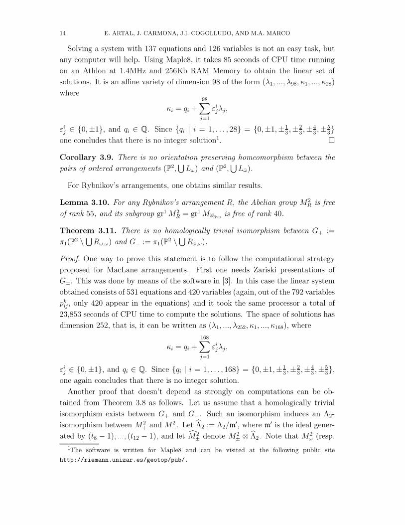
Solving a system with 137 equations and 126 variables is not an easy task, but
any computer will help. Using Maple8, it takes 85 seconds of CPU time running
on an Athlon at 1.4MHz and 256Kb RAM Memory to obtain the linear set of
solutions. It is an affine variety of dimension 98 of the form (λ1, ..., λ98, κ1, ..., κ28)
where
κi = qi +
98∑
j=1
εijλj,
εij ∈ {0,±1}, and qi ∈ Q. Since {qi | i = 1, . . . , 28} = {0,±1,±13,±2
3,±4
3,±5
3}
one concludes that there is no integer solution1. �
Corollary 3.9. There is no orientation preserving homeomorphism between the
pairs of ordered arrangements (P2,⋃Lω) and (P2,
⋃Lω).
For Rybnikov’s arrangements, one obtains similar results.
Lemma 3.10. For any Rybnikov’s arrangement R, the Abelian group M2R is free
of rank 55, and its subgroup gr1M2R = gr1MCRyb
is free of rank 40.
Theorem 3.11. There is no homologically trivial isomorphism between G+ :=
π1(P2 \
⋃Rω,ω) and G− := π1(P
2 \⋃Rω,ω).
Proof. One way to prove this statement is to follow the computational strategy
proposed for MacLane arrangements. First one needs Zariski presentations of
G±. This was done by means of the software in [3]. In this case the linear system
obtained consists of 531 equations and 420 variables (again, out of the 792 variables
pkij, only 420 appear in the equations) and it took the same processor a total of
23,853 seconds of CPU time to compute the solutions. The space of solutions has
dimension 252, that is, it can be written as (λ1, ..., λ252, κ1, ..., κ168), where
κi = qi +
168∑
j=1
εijλj,
εij ∈ {0,±1}, and qi ∈ Q. Since {qi | i = 1, . . . , 168} = {0,±1,±13,±2
3,±4
3,±5
3},
one again concludes that there is no integer solution.
Another proof that doesn’t depend as strongly on computations can be ob-
tained from Theorem 3.8 as follows. Let us assume that a homologically trivial
isomorphism exists between G+ and G−. Such an isomorphism induces an Λ2-
isomorphism between M2+ and M2
−. Let Λ2 := Λ2/m′, where m
′ is the ideal gener-
ated by (t8 − 1), ..., (t12 − 1), and let M2± denote M2
± ⊗ Λ2. Note that M2ω (resp.
1The software is written for Maple8 and can be visited at the following public site
http://riemann.unizar.es/geotop/pub/.

COMBINATORIAL LINE ARRANGEMENTS 15
M2ω) can be considered as the Λ2-module obtained from the inclusion of the com-
plements P2 \⋃Rω,ω →P2 \
⋃Lω (resp. P2 \
⋃Rω,ω →P2 \
⋃Lω). Moreover, these
inclusions define epimorphisms of Λ2-modules π : M2+ ։ M2
ω and π : M2+ ։ M2
ω.
Proving the existence of a homologically trivial isomorphism h2 that matches in
the commutative diagram (11), and using Theorem 3.8 one obtains a contradiction.
(11)
M2+
h2
−→ M2−
π ↓ ↓ π
M2ω
h2
→→ M2ω
Consider S+ the Λ2-submodule of M2+ generated by the elements xi,j , i, j ∈
{1, ..., 7} and consider the commutative diagram (12). Since π(xi,j) = xi,j and
h2(xi,j) ≡ xi,j mod gr1M2ω.
(12)
M2+
h2
−→ M2−
π → ↓ π
S+h2
→→ M2ω
π|→→
M2ω
Since M2ω and M2
ω are free Abelian of the same rank, (11) can be obtained from
(12), by proving that π| is an isomorphism, which is the statement of Lemma 3.12.
�
Lemma 3.12. The epimorphism π| in (12) is injective
Proof. We break the proof in several steps.
(O1) (tk − 1)xi,j = 0 in M2+ if {i, j} ∩ {8, ..., 12} 6= ∅.
This can be proved case by case (all the equalities are considered in M2+):
(a) If i ∈ {3, ..., 7} and j ∈ {8, ..., 12} (or vice versa, since xi,j = −xj,i): this
is a consequence of Example 2.9(1) since the lines ℓi and ℓj intersect
transversally.
(b) If i, j ∈ {8, ..., 12}: this is a consequence of (a) and the Jacobi relations
(Property 2.2(6)).
(c) If i ∈ {1, 2}, j ∈ {8, ..., 12}: using the Jacobi relations (Property 2.2(6))
and (b) it is enough to check that (tk − 1)xi,j = 0, i, k ∈ {1, 2}, j ∈
{8, ..., 12}. If ℓi and ℓj intersect at a double point, then (a) proves the
result. Otherwise, there exists a line ℓm (m ∈ {7, ..., 12}) such that
ℓi, ℓj and ℓm intersect at a triple point. By Example 2.9(2) one has
(tk − 1)xi,j + (tk − 1)xm,j = 0, but (tk − 1)xm,j = 0 by (b), thus we are
done.

16 E. ARTAL, J. CARMONA, J.I. COGOLLUDO, AND M.A. MARCO
(O2) gr1(M2+) ⊂ S+. It is a direct consequence of (O1).
(O3) gr0(M2+) =
S+
gr1 M2+
⊕ker π + gr1 M2
+
gr1 M2+
, i.e.,S+
gr1 M2+
∼= gr0M2ω.
Since ker π is generated by 〈xi,j〉1≤i<j≤12,j>7, it is clear that gr0(M2+) de-
composes in the required sum. It remains to prove that it is a direct sum.
One can consider gr0(M2+) as a quotient
〈xi,j〉1≤i<j≤12
W, hence it is enough
to check that there is a system of generators r1, ..., rn of W such that:
(*) either ri ∈ker π + gr1 M2
+
gr1 M2+
, or ri ∈S+
gr1 M2+
.
Note that a system of relators can be obtained combinatorially as xi,j = 0
(if {ℓi, ℓj} is a double point) or xi,j +xi,k = 0 (if {ℓi, ℓj, ℓk} is a triple point).
Relations coming from double points satisfy (*). For the triple point relations
note that any triple point {ℓi, ℓj, ℓk} such that {i, j} ⊂ {8, ..., 12}, verifies
that k ∈ {8, ..., 12}; therefore, condition (*) is also satisfied.
(O4) gr1(M2+) ∼= gr1M2
ω.
By (O1), the Abelian group M2+ is generated by xi,j , i, j ∈ {1, . . . , 12}, and
(tk − 1)xi,j, i, j, k ∈ {1, . . . , 7}; the relators are obtained from the singular
points (see Example 2.9) and the Jacobi relations J .
By (O1) and Remark 3.6, we find that gr1(M2+) is generated by the el-
ements (tk − 1)xi,j, i, j, k ∈ {1, . . . , 7} and the relations are exactly those
in J and the relations (5) and (7) in Example 2.9. The arguments used in
(O3) also show that only double and triple points in CML provide non-trivial
relations and thus one obtains the same system of generators and relations
of gr1M2ω.
�
Remark 3.13. The proof of Lemma 3.12 is combinatorial and depends strongly on
the properties of CRyb. This lemma corresponds to a key statement of the proof
of [5, Lemma 4.3] which is worth mentioning.
4. Homologically Trivial Fundamental Groups
This last section will be devoted to proving that the fundamental groups of Rω,ω
and Rω,ω are not isomorphic.
Remark 4.1. Associated with a combinatorial type C := (L,P), there is a family
of groups, where
HC :=
⊕ℓ∈L〈xℓ〉Z
〈∑
ℓ∈L xℓ〉Z
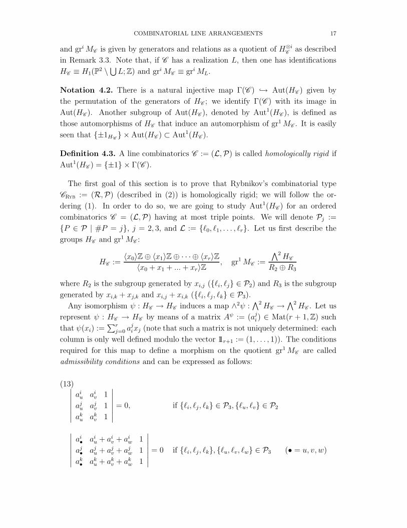
COMBINATORIAL LINE ARRANGEMENTS 17
and griMC is given by generators and relations as a quotient of H⊗iC
as described
in Remark 3.3. Note that, if C has a realization L, then one has identifications
HC ≡ H1(P2 \
⋃L; Z) and griMC ≡ griML.
Notation 4.2. There is a natural injective map Γ(C ) → Aut(HC ) given by
the permutation of the generators of HC ; we identify Γ(C ) with its image in
Aut(HC ). Another subgroup of Aut(HC ), denoted by Aut1(HC ), is defined as
those automorphisms of HC that induce an automorphism of gr1MC . It is easily
seen that {±1HC} × Aut(HC ) ⊂ Aut1(HC ).
Definition 4.3. A line combinatorics C := (L,P) is called homologically rigid if
Aut1(HC ) = {±1} × Γ(C ).
The first goal of this section is to prove that Rybnikov’s combinatorial type
CRyb := (R,P) (described in (2)) is homologically rigid; we will follow the or-
dering (1). In order to do so, we are going to study Aut1(HC ) for an ordered
combinatorics C = (L,P) having at most triple points. We will denote Pj :=
{P ∈ P | #P = j}, j = 2, 3, and L := {ℓ0, ℓ1, . . . , ℓr}. Let us first describe the
groups HC and gr1MC :
HC :=〈x0〉Z ⊕ 〈x1〉Z ⊕ · · · ⊕ 〈xr〉Z
〈x0 + x1 + ... + xr〉Z, gr1MC :=
∧2HC
R2 ⊕ R3
where R2 is the subgroup generated by xi,j ({ℓi, ℓj} ∈ P2) and R3 is the subgroup
generated by xi,k + xj,k and xi,j + xi,k ({ℓi, ℓj, ℓk} ∈ P3).
Any isomorphism ψ : HC → HC induces a map ∧2ψ :∧2HC →
∧2HC . Let us
represent ψ : HC → HC by means of a matrix Aψ := (aji ) ∈ Mat(r + 1,Z) such
that ψ(xi) :=∑r
j=0 ajixj (note that such a matrix is not uniquely determined: each
column is only well defined modulo the vector 11r+1 := (1, . . . , 1)). The conditions
required for this map to define a morphism on the quotient gr1MC are called
admissibility conditions and can be expressed as follows:
(13)∣∣∣∣∣∣∣
aiu aiv 1
aju ajv 1
aku akv 1
∣∣∣∣∣∣∣= 0, if {ℓi, ℓj , ℓk} ∈ P3, {ℓu, ℓv} ∈ P2
∣∣∣∣∣∣∣
ai• aiu + aiv + aiw 1
aj• aju + ajv + ajw 1
ak• aku + akv + akw 1
∣∣∣∣∣∣∣= 0 if {ℓi, ℓj , ℓk}, {ℓu, ℓv, ℓw} ∈ P3 (• = u, v, w)

18 E. ARTAL, J. CARMONA, J.I. COGOLLUDO, AND M.A. MARCO
(also note that such conditions are invariant on the coefficient vectors (a0•, a
1•, ..., a
12• )
modulo 1113). We summarize these facts.
Proposition 4.4. Any morphism ψ : HC → HC whose associated matrix Aψ
satisfies the admissibility conditions (13) produces a well-defined morphism ∧2ψ :
M1C→ M1
C.
We are going to express the admissibility conditions (13) in a more useful way.
Let ψ ∈ Aut1(HC ) and let Aψ be a matrix representing ψ. Fix P ∈ P3 and consider
the submatrix AψP ∈ Mat(3×12,Z) of Aψ which contains the rows associated with
P . Let Σk := Zk+1/11k+1, k ∈ N. We denote by v0(P ), v1(P ) . . . , vr(P ) ∈ Σ2, the
column vectors (mod 113) of AψP .
Lemma 4.5.
(1) The vectors v0(P ), v1(P ) . . . , vr(P ) span Σ2.
(2)∑r
j=0 vj(P ) = 0 ∈ Σ2.
(3) For any Q ∈ P and for any ℓu ∈ Q, the vectors vu(P ) and∑
ℓi∈Qvi(P )
are linearly dependent (i.e., span a sublattice of Σ2 of rank less than two).
In particular, if∑
ℓi∈Qvi(P ) 6= 0, then {vi(P ) | ℓi ∈ Q} spans a rank-one
sublattice of Σ2.
(4) There exists Q ∈ P3 such that {vi(P ) | ℓi ∈ Q} spans a rank-two sublattice of
Σ2 and∑
ℓi∈Qvi(P ) = 0.
Proof.
(1) ψ is an automorphism.
(2) The sum of the columns of Aψ is a multiple of 11r+1.
(3) It is an immediate consequence of the admissibility conditions (13).
(4) If no such Q exists, then all the vectors Vi(P ) are linearly dependent, which
contradicts (1). The last part is a consequence of (3).
�
Definition 4.6. Let C := (L,P) be a combinatorics; we say C ′ := (L′,P ′) is a
subcombinatorics of C if L′ ⊂ L and P ′ := {P ∩ L | P ∈ P,#(P ∩ L) ≥ 2}.
We define a subcombinatorics Admψ(P ) ⊂ C as follows:
L(Admψ(P )) := {ℓi ∈ R | vi(P ) 6= 0}.
Note that,
(14) ℓi /∈ L(Admψ(P )) ⇐⇒ the ith column of AψP is a multiple of 113 .
This motivates the following definition.

COMBINATORIAL LINE ARRANGEMENTS 19
Definition 4.7. A line combinatorics C := (L,P) with only double and triple
points is called 3-admissible if it is possible to assign a non-zero vector vi ∈ Z2 to
each ℓi ∈ L such that:
(1) There exists P ∈ P3, such that {vj | ℓj ∈ P} spans a rank-two sublattice.
(2) For every P ∈ P and for every ℓi ∈ P , vi and∑
ℓj∈Pvj are linearly depen-
dent.
(3)∑
ℓi∈Lvi = (0, 0).
Remarks 4.8. The conditions of Definition 4.7 can be made more precise.
(1) If P = {ℓi, ℓj} ∈ P2, then vi and vj are proportional, in notation, vi‖vj .
(2) If P ∈ P3 verifies condition (1) then∑
ℓi∈Pvi = (0, 0).
Examples 4.9.
(1) With the above notation, Admψ(P ) is 3-admissible by Lemma 4.5.
(2) The combinatorics M3 of a triple point (that is, LM3 := {0, 1, 2}, PM3 :=
{{0, 1, 2}}) is 3-admissible, simply using v0 := (1, 0), v1 := (0, 1), v2 :=
(−1,−1).
(3) Let C := (L,P) be a combinatorics such that
• L := L0
∐L1
∐L2;
• L1 and L2 define non-empty subcombinatorics in general position
w.r.t. L0 (that is, ℓi ∈ L1 and ℓj ∈ L2 implies that {ℓi, ℓj} ∈ P);
• at most one line of L0 intersects L1 ∪ L2 in a non-multiple point of
L0.
Then C is not 3-admissible. It is enough to see that if {vi}ℓi∈L is a set of
non-zero vectors satisfying conditions (2) and (3) of Definition 4.7, one has
that vi‖vj.
• ℓi ∈ L1 and ℓ2 ∈ L2; since {ℓi, ℓj} ∈ P then, by Remark 4.8(1), vi‖vj .
• ℓi, ℓj ∈ L1; considering any ℓk ∈ L2 and using the previous case, one
has vi‖vk‖vj. The same argument works for ℓi, ℓj ∈ L2. In particular,
vi‖vj if ℓi, ℓj ∈ L1 ∪ L2.
• ℓi ∈ L0 and P ∈ P such that P ∩ L0 = {ℓi}. Since all the vectors
associated with P but one are proportional, then this must also be
the case for vi.
All the vectors (but at most one) are proportional. To conclude we apply
condition (3) of Definition 4.7.
(4) Ceva’s line combinatorics is 3-admissible.
Proof. Ceva’s line combinatorics is given by the following realization:
Lceva := {1, 2, 3, 4, 5, 6}

20 E. ARTAL, J. CARMONA, J.I. COGOLLUDO, AND M.A. MARCO
ℓ2ℓ4
ℓ5
ℓ6
ℓ3
ℓ1
Figure 2. Ceva’s line combinatorics
Pceva := {{1, 2}, {3, 4}, {5, 6}, {1, 3, 5}, {1, 4, 6}, {2, 3, 6}, {2, 4, 5}}.
For example, the following is a 3-admissible set of vectors for Ceva:
{v1 = v2 = (1, 0), v3 = v4 = (0, 1), v5 = v6 = (−1,−1)}
�
(5) MacLane’s line combinatorics CML is not 3-admissible.
Proof. We will use the combinatorics given in Figure 1. Let us assume that
MacLane is 3-admissible, then one has a list of non-zero vectors v0, v1, ..., v7
associated with each line. We will first see that v0 and v1 cannot be pro-
portional. If they were (v0‖v1), using {0, 1, 2}, {1, 6} and {2, 3} one would
have that v0‖v2‖v6‖v3 and finally, using {3, 6, 7}, one obtains v0‖v7, and
hence, by {1, 4, 7} and {4, 5}, all vectors are proportional, which contra-
dicts condition (1) of Definition 4.7.
Therefore, v0 and v1 are linearly independent. After a change of basis,
one can assume that v0 = (α, 0), v1 = (0, β), α, β ∈ Z \ {0}, and therefore
v2 = (−α,−β). We will briefly describe the conditions and how they affect
the vectors until a contradiction is reached:{0, 7}
{1, 6}→
v7 = (γ, 0)
v6 = (0, δ)
{3, 6, 7}
{0, 5, 6}→
v3 = (−γ,−δ)
v5 = (−α,−δ)
{1,3,5}→
α = −γ
β = 2δ.
Hence v3 does not satisfy the condition (2) of Definition 4.7 with v2 =
(γ,−2δ) on the double point {2, 3}. �
Definition 4.10. A combinatorics C with only double and triple points is point-
wise 3-admissible if the only 3-admissible subcombinatorics of C are isomorphic
to M3.

COMBINATORIAL LINE ARRANGEMENTS 21
Proposition 4.11. If C is a pointwise 3-admissible combinatorics then any ψ ∈
Aut1(HC ) induces a permutation ψ3 of P3.
Proof. Let L := {ℓ0, ..., ℓr} denote the set of lines of C and let P3 ⊂ P denote the
set of triple points of C . We will first prove that any isomorphism ψ ∈ Aut1(HC )
induces a map ψ3 : P3 → P3. Consider a triple point P := {ℓi, ℓj, ℓk} ∈ P3; then
Admψ(P ) is an admissible subcombinatorics of C (Example 4.9(1)) and defines a
triple point. The map ψ3 : P3 → P3 given by ψ3(P ) := Admψ(P ) is defined.
We will next prove that such a map is indeed injective, and hence a permutation
(in order for this to make sense, one has to assume that #P3 > 1 and hence r ≥ 4).
Assume ψ3 is not injective, and let ψ3(P1) = ψ3(P2) = Q = {ℓu, ℓv, ℓw}. One has
to consider two different cases depending on whether or not P1 and P2 share a
line:
(1) If P1, P2 do not share a line, i.e, P1 := {ℓi1 , ℓj1, ℓk1} and P2 := {ℓi2 , ℓj2, ℓk2},
where all the subscripts are pairwise different. By reordering the columns,
let us write Q = {ℓ0, ℓ1, ℓ2}. Let AψP1,P2be the submatrix of Aψ correspond-
ing to the rows {i1, j1, k1, i2, j2, k2}. Using (14):
(15) AψP1,P2:=
ai10 ai11 ai12 ai13 . . . ai1raj10 aj11 aj12 ai13 . . . ai1rak10 ak11 ak12 ai13 . . . ai1rai20 ai21 ai22 ai23 . . . ai2raj20 aj21 aj22 ai23 . . . ai2rak20 ak21 ak22 ai23 . . . ai2r
,
where ai•0 + ai•1 + ai•2 = aj•0 + aj•1 + aj•2 = ak•0 + ak•1 + ak•2 , • = 1, 2. The sub-
lattice K of Σ5 generated by the columns (mod 116) should have maximal
rank equal to 5. Note that rank (K) equals the rank of the matrix Aψ
P1,P2
obtained by subtracting the last row from the first ones, forgetting the last
row and replacing the first column by the sum of the first three:
(16) Aψ
P1,P2=
bi10 bi11 b2 b3 . . . brbj10 bj11 b2 b3 . . . br
bk10 bk11 b2 b3 . . . brbi20 bi21 0 0 . . . 0
bj20 bj21 0 0 . . . 0
,
which does not have rank 5.
(2) If P1, P2 share a line, say P1 := {i, j1, k1} and P1 := {i, j2, k2}. Then,
analogously to the previous case, one obtains a similar matrix to (15) but
where the rows i1 and i2 are identified, and we proceed in a similar way.

22 E. ARTAL, J. CARMONA, J.I. COGOLLUDO, AND M.A. MARCO
�
Definition 4.12. Three triple points P,Q,R ∈ P of a line combinatorics (L,P)
are said to be in a triangle if P ∩Q = {ℓ1}, P ∩ R = {ℓ2} and Q ∩ R = {ℓ3} are
pairwise different.
Proposition 4.13. For any ψ ∈ Aut1(HC ), C pointwise 3-admissible, ψ3 satisfies
the following Triangle Property: ψ3 : P3 → P3 preserves triangles, that is, if
P1, P2, P3 ∈ P3 are in a triangle, then ψ3(P1), ψ3(P2), ψ3(P3) are also in a triangle.
Proof. Let P1, P2, P3 ∈ P3 be three triple points in a triangle, say P1 := {ℓi, ℓj, ℓk},
P2 := {ℓk, ℓl, ℓm}, P3 := {ℓm, ℓn, ℓi}. Let us assume that ψ3(P1), ψ3(P2), ψ3(P3) are
not in a triangle. One has two possibilities, either two of them do not share a line
or three of them share a line.
(1) Two of them, say ψ3(P1), ψ3(P2) do not share a line. After reordering, we
can suppose that ψ3(P1) = {ℓ0, ℓ1, ℓ2} and ψ3(P2) = {ℓ3, ℓ4, ℓ5}. For ψ3(P3)
there are several possibilities but we may assume ψ3(P3) ⊂ {ℓ0, ℓ3, ℓ6, ℓ7, ℓ8}.
Consider the submatrix AψP1,P2,P3of Aψ given by the rows of P1, P2, P3. Ap-
plying (14) successively to the rows defined by P1, P2, P3 one has:
(17) AψP1,P2,P3:=
ai0 ai1 ai2 a3 a4 a5 a6 a7 a8 a9 . . . araj0 aj1 aj2 a3 a4 a5 a6 a7 a8 a9 . . . ar
a0 a1 a2 a3 a4 a5 a6 a7 a8 a9 . . . ara0 a1 a2 al3 al4 al5 a6 a7 a8 a9 . . . ar
a0 a1 a2 am3 a4 a5 a6 a7 a8 a9 . . . aran0 a1 a2 an3 a4 a5 an6 an7 an8 a9 . . . ar
;
moreover, ai1 = a1, ai2 = a2,
ai0 + a1 + a2 = aj0 + aj1 + aj2 = a0 + a1 + a2(⇒ ai0 = a0),
a3 + a4 + a5 = al3 + al4 + al5= am3 + a4 + a5(⇒ am3 = a3)
and
a0 + a3 + a6 + a7 + a8 = an0 + an3 + an6 + an7 + an8 .
As in the proof of Proposition 4.11 we need rank (Aψ
P1,P2,P3) = 5, where
Aψ
P1,P2,P3is the matrix obtained from AψP1,P2,P3
by subtracting the last row

COMBINATORIAL LINE ARRANGEMENTS 23
from the first ones and forgetting the last row. We obtain:
(18) AψP1,P2,P3:=
b0 0 0 b3 0 0 b6 b7 b8 0 . . . 0
bj0 bj1 bj2 b3 0 0 b6 b7 b8 0 . . . 0
b0 0 0 b3 0 0 b6 b7 b8 0 . . . 0
b0 0 0 bl3 bl4 bl5 b6 b7 b8 0 . . . 0
b0 0 0 b3 0 0 b6 b7 b8 0 . . . 0
which cannot have rank 5.
(2) If ψ3(P1), ψ3(P2) and ψ3(P3) have a common line, say ℓ0, we follow the
same strategy and obtain the desired result.
�
Our main goal is to check if ψ3 is induced by an element of Aut(C ). The next
example shows that we need enough triangles.
Example 4.14. Note that Proposition 4.11 does not automatically ensure that in
general an automorphism of the combinatorics is produced. For instance, consider
the combinatorics C given by the lines {0, 1, . . . , 6}, and the following triple points
{0, 1, 2}, {2, 3, 4}, and {4, 5, 6} (the remaining intersections are double points). It
is easy to see that such a combinatorics is pointwise 3-admissible. Let ψ : HC →
HC be given by the following matrix:
Aψ :=
1 0 0 0 0 0 0
0 1 0 0 0 0 0
0 0 1 0 0 0 0
0 0 1 0 1 0 −1
0 0 1 0 0 1 −1
0 0 0 1 0 1 −1
0 0 0 0 1 1 −1
,
satisfying the admissibility relations. This induces the following maps:
P3ψ3→ P3
{0, 1, 2} 7→ {0, 1, 2}
{2, 3, 4} 7→ {4, 5, 6}
{4, 5, 6} 7→ {2, 3, 4}
gr1MC
∧2ψ→ gr1MC
x0,1 7→ x0,1
x2,3 7→ x4,5
x4,5 7→ x2,3,
where gr1MC∼= 〈x0,1〉Z ⊕ 〈x2,3〉Z ⊕ 〈x4,5〉Z.
However, the given permutation is not induced by an automorphism of the
combinatorics, because the point {2, 3, 4} (which is the only one that shares a line
with the other two) is not fixed.

24 E. ARTAL, J. CARMONA, J.I. COGOLLUDO, AND M.A. MARCO
We want to apply the previous results to CRyb. First we will check that CRyb is
pointwise 3-admissible.
Lemma 4.15. An admissible subcombinatorics of CRyb cannot have lines in both
R1 := {3, 4, 5, 6, 7} and R2 := {8, 9, 10, 11, 12}.
Proof. Any subcombinatorics of CRyb having lines in both R1 and R2 verifies the
conditions of Example 4.9(3). �
Lemma 4.16. CML is pointwise 3-admissible.
Proof. It is not difficult to prove that any combinatorics (with only double and
triple points) of less than 6 lines (other than M3) is not 3-admissible. In Exam-
ple 4.9(5) it is shown for the whole combinatorics of eight lines. Let us check the
remaining cases, that is, six and seven lines. Note that, up to a combinatorics
automorphism, there is a unique way to remove one line. There are, however, two
possible ways to remove two lines, depending on whether they intersect or not at
a triple point. Therefore we only have to check the following cases:
(1) For 7 lines
{0, 1, 2, 3, 4, 5, 6}:{3,6}→ v3‖v6
{1,6},{2,3}→ v3‖v1‖v2
{1,4}→ v3‖v4
{4,5}→ v3‖v5.
(2) For 6 lines, removing two lines intersecting at a triple point
{0, 2, 3, 4, 5, 6}:{3,5}→ v5‖v3
{2,3},{3,6},{4,5}→ v5‖v2‖v6‖v4.
(3) For 6 lines, removing two lines intersecting at a double point
{0, 2, 3, 4, 5, 7}:{2,3},{2,4}
→ v2‖v3‖v4{3,7},{4,5}
→ v2‖v5‖v7.
�
Proposition 4.17. CRyb is pointwise 3-admissible.
Proof. An immediate consequence of Lemmas 4.15 and 4.16. �
Remarks 4.18. In order to prove that for any ψ ∈ Aut1(HCRyb), ψ3 comes from an
element of Aut(CRyb) we need to know more combinatorial properties of CRyb and
CML.
(1) The triple point {0, 1, 2} ∈ P3 in CRyb is the only one that belongs to 36
triangles.
(2) Any triple point P ∈ P3 in CRyb except for {3, 6, 7} and {8, 11, 12} satisfies
that {0, 1, 2} and P are in a triangle.
(3) Any two triple points in CML sharing a line belong to a triangle.
(4) For any three triple points P1, P2, P3 in CML, there exists another triple
point Q such that Q,Pi, Pj belong to a triangle (i, j ∈ {1, 2, 3}).
Proposition 4.19. Let ψ ∈ Aut1(CRyb).

COMBINATORIAL LINE ARRANGEMENTS 25
(1) ψ3({0, 1, 2}) = {0, 1, 2}
(2) ψ3 either preserves (resp. exchanges) the triple points of R1 and R2 in CRyb
inducing an automorphism
(3) The action of ψ3 on R1 and R2 comes from an automorphism (resp. isomor-
phism) of their combinatorics.
Proof. Part (1) is true by Propositions 4.11-4.13 and Remark 4.18(1). By Re-
mark 4.18(2), the points {3, 6, 7} and {8, 11, 12} are either preserved or exchanged.
In order to prove (2) and (3), we may suppose that ψ3({3, 6, 7}) = {3, 6, 7}. Re-
call that the subcombinatorics defined by R0 ∪ R1 is isomorphic to CML. Since
triangles are preserved by ψ3 (Proposition 4.13), according to Remark 4.18(3) the
images of any two triple points in R0 ∪ R1 sharing a line also share a line. This
implies, using Remark 4.18(4) again, that the image of any three triple points on
R0 ∪ R1 sharing a line are also three points sharing a line. Since any line in R1
or R2 has at least three triple points, we conclude (2) and (3). �
Proposition 4.20. Let ψ ∈ Aut1(HCRyb); then ψ3 : P3 → P3 is induced by an
automorphism of CRyb.
Proof. We will use Proposition 4.19 repeatedly. We can compose ψ with an ele-
ment of Aut(CRyb) in order to have ψ3 preserve the triple points in Ri. Recall that
ψ3|R0∪Ricomes from an automorphism ϕi of CML which respects {0, 1, 2}. Com-
posing again with an element of Aut(CRyb) we may suppose that ϕ1 is the identity
on {0, 1, 2}. It is enough to prove that it is also the case for ϕ2. If it is not the case,
we may assume (by conjugation with an element of Aut(CRyb)) that ϕ2(0) = 1.
There are two possibilities to be checked, depending on whether 9 and 10 are fixed
or permuted. In both cases, the triple points {0, 1, 2}, {3, 6, 7} and {8, 11, 12} are
fixed. Using the arguments in the proofs of Propositions 4.11 and 4.13, one can
obtain the induced matrices Aψ with all the admissibility relations, which, modulo
1113 do not have a maximal rank in either case. �
Proposition 4.21. CRyb is homologically rigid.
Proof. Let ψ ∈ Aut1(HCRyb); by Propositions 4.20 and 4.13, ψ3 comes from an
automorphism of the combinatorics. Composing with the inverse of such an au-
tomorphism, we may suppose that ψ3 = 1P3 . It is hence enough to prove that
any isomorphism ψ ∈ Aut1(HCRyb) that induces the identity on ψ3 is just ±1HCRyb
.
From the definition of Admψ(P ), P ∈ P3, we deduce the following. Let us fix
the jth-column; all the entries in this column corresponding to P ∈ P3 such that
j /∈ P are equal. We deduce from this that we can choose Aψ such that all the
elements outside the diagonal are constant in their column. Adding multiples of

26 E. ARTAL, J. CARMONA, J.I. COGOLLUDO, AND M.A. MARCO
1113, we obtain that Aψ can be chosen to be diagonal. We also know that for
each P ∈ P3, the diagonal terms corresponding to P are equal and since any two
elements can be joined by a chain of triple points, we deduce that all the diagonal
terms are equal. Since ψ is an automorphism, they are equal to ±1 and then
ψ = ±1HCRyb. �
Therefore we can prove the main result.
Theorem 4.22. The fundamental groups of the two complex realizations of Ryb-
nikov’s combinatorics are not isomorphic.
Proof. Let G+ and G− be the fundamental groups of Rω,ω and Rω,ω respectively.
Any isomorphism ψ : G+ → G− will produce an automorphism ψ : HCRyb≡
G+/G′+ → G−/G
′− ≡ HCRyb
, that is, we can consider ψ ∈ Aut1(CRyb). By
Theorem 4.21, ψ induces an automorphism of CRyb. Since the identifications
HCRyb≡ G±/G
′± are made up to the action of Aut(CRyb), we may assume that
ψ induces ±1HCRyb. Moreover, eventually exchanging Rω,ω (resp. Rω,ω) for Rω,ω
(resp. Rω,ω), see Example 1.10 by means of the automorphism given by complex
conjugation, we may assume that ψ = 1HCRyb(Proposition 4.21). Therefore ψ is a
homologically trivial isomorphism between G+ and G−, something which is ruled
out by Theorem 3.11. �
References
[1] D. Arapura, Geometry of cohomology support loci for local systems I, J. of Alg. Geom. 6
(1997), 563–597.
[2] E. Artal, J. Carmona, J.I. Cogolludo, and M. Marco, Topology and combinatorics of real line
arrangements, Preprint available at arXiv:math.AG/0307296, 2003.
[3] J. Carmona, Monodromıa de trenzas de curvas algebraicas planas, Ph.D. thesis, Universidad
de Zaragoza, 2003.
[4] A. Libgober, Characteristic varieties of algebraic curves, Applications of algebraic geometry
to coding theory, physics and computation (Eilat, 2001), Kluwer Acad. Publ., Dordrecht,
2001, pp. 215–254.
[5] G. Rybnikov, On the fundamental group of the complement of a complex hyperplane arrange-
ment, Preprint available at arXiv:math.AG/9805056.

COMBINATORIAL LINE ARRANGEMENTS 27
Departamento de Matematicas, Campus Plaza de San Francisco s/n, E-50009
Zaragoza SPAIN
E-mail address : [email protected]
Departamento de Sistemas informaticos y programacion, Universidad Complu-
tense, Ciudad Universitaria s/n, E-28040 Madrid SPAIN
E-mail address : [email protected]
Departamento de Matematicas, Campus Plaza de San Francisco s/n, E-50009
Zaragoza SPAIN
E-mail address : [email protected]
Departamento de Matematicas, Campus Plaza de San Francisco s/n, E-50009
Zaragoza SPAIN
E-mail address : [email protected]