Innovative Water Supply Reliability Arrangements

INNOVATIVE WATER SUPPLY RELIABILITY ARRANGEMENTS

by

Michael O’Donnell

A Thesis Submitted to the Faculty of the

DEPARTMENT OF AGRICULTURAL AND RESOURCE ECONOMICS

In Partial Fulfillment of the Requirements For the Degree of

MASTER OF SCIENCE

2

STATEMENT BY AUTHOR This Thesis has been submitted in partial fulfillment of requirements for an advanced degree at The University of Arizona and is deposited in the University Library to be made available to borrowers under rules of the Library. Brief quotations from this thesis are allowable without special permission, provided that accurate acknowledgment of source is made. Requests for permission for extended quotation from or reproduction of this manuscript in whole or in part may be granted by the head of the major department or the Dean of the Graduate College when in his or her judgment the proposed use of the material is in the interests of scholarship. In all other instances, however, permission must be obtained from the author

SIGNED: ___________________________

APPROVAL BY THESIS DIRECTOR

This thesis has been approved on the date shown below:

_______________________________________ ____________________________ Bonnie G. Colby Date Professor Agricultural and Resource Economics

3

ACKNOWLEDGEMENTS

4

DEDICATION

5

ABSTRACT .................................................................................................................................................................... 7 LIST OF TABLES AND FIGURES .............................................................................................................................. 8 1. INTRODUCTION AND BACKGROUND ............................................................................................................... 9

1.1 ECONOMICS OF DROUGHT .................................................................................................12 1.2 DESCRIPTION OF CHAPTERS ..............................................................................................13

2. LITERATURE REVIEW ........................................................................................................................................ 15 2.1 WATER MARKETS ..............................................................................................................15 2.2 ECONOMETRIC ANALYSIS OF WATER TRANSFERS .............................................................17 2.3 NET RETURNS OVER VARIABLE COST (NROVC) ..............................................................21 2.4 CONTRIBUTION ..................................................................................................................23

3. LAW AND ECONOMICS REVIEW OF US WATER LAW ............................................................................... 25 3.1 US HISTORY OF LEGAL REGIMES ......................................................................................25 3.1.1 Early British Riparian Water Law and Economics ................................................................................. 25 3.1.2 Early Colonial Riparianism and Reasonable Use ................................................................................... 29 3.1.3 Western Expansion and Prior Appropriation .......................................................................................... 33 3.1.4 “Mixed” Water Systems ........................................................................................................................... 36 3.1.5 Summary ................................................................................................................................................... 43 3.2 MODERN DEVELOPMENTS .................................................................................................44 3.3 ECONOMICS AND COMPLICATIONS OF WATER TRANSFERS ...............................................45

4. DRY-YEAR WATER SUPPLY RELIABILITY CONTRACTS ......................................................................... 48 4.1 RELIABILITY CONTRACT BACKGROUND .............................................................................48 4.2 DRY-YEAR RELIABILITY CONTRACT EXAMPLES ................................................................52 4.3 STRUCTURING THE RELIABILITY CONTRACT .....................................................................55 4.4 TRIGGER MECHANISMS .....................................................................................................59 4.5 MONITORING AND EVALUATION ........................................................................................61 4.6 SUMMARY ..........................................................................................................................64

5. WATER AUCTION DESIGN FOR SUPPLY RELIABILITY ............................................................................ 65 5.1 WATER AUCTION BACKGROUND ........................................................................................65 5.2 OVERVIEW OF WATER AUCTION DESIGN ..........................................................................70 5.3 SEALED BID MULTIPLE-UNIT PROCUREMENT WATER AUCTIONS ....................................71 5.4 POSSIBLE MODIFICATIONS TO THE TYPICAL WATER AUCTION DESIGN ...........................76 5.5 POST AUCTION COMPLIANCE AND EVALUATION ...............................................................80 5.6 SUMMARY ..........................................................................................................................82

6. WATER BANKING ................................................................................................................................................. 84 6.1 WATER BANKING BACKGROUND ........................................................................................84 6.2 WATER BANKING CREATION AND OPERATION ..................................................................88 6.3 EXAMPLES OF WATER BANKS ............................................................................................96 6.4 SUMMARY ........................................................................................................................109

7. DATA DESCRIPTION AND ECONOMETRIC MODEL ................................................................................. 111 7.1 DATA DESCRIPTION AND BACKGROUND ..........................................................................111 7.1.2 Data Cleaning ......................................................................................................................................... 114 7.2 SUMMARY STATISTICS .....................................................................................................116 7.2.1 Price Data ............................................................................................................................................... 116

6

7.2.2 Transaction Data .................................................................................................................................... 118 7.2.2 Median Home Price Data ....................................................................................................................... 123 5.2.3 Precipitation Data ................................................................................................................................... 125 7.2.4 Temperature Data ................................................................................................................................... 126 7.2.5 Climate Variables ................................................................................................................................... 127 7.2.6 Population and Income .......................................................................................................................... 128 7.2.7 Lake Mead Elevation .............................................................................................................................. 130 7.3 ECONOMETRIC MODEL - INTRODUCTION ........................................................................130 7.4 SUMMARY OF VARIABLES ................................................................................................133

8. RESULTS AND ANALYSIS ................................................................................................................................. 137 8.1 ECONOMETRIC RESULTS..................................................................................................137 8.1.1 Three States Model Results .................................................................................................................... 138 8.1.2 California Model Results ....................................................................................................................... 139 8.1.3 Colorado Model Results ......................................................................................................................... 140 8.1.4 New Mexico Model Results .................................................................................................................... 141 8.2 ANALYSIS .........................................................................................................................142 8.3 INTERPRETATION OF RESULTS ........................................................................................150

9. NET RETURNS OVER VARIABLE COST AND PILOT PROGRAMS ......................................................... 153 9.1 YUMA COUNTY NROVC ..................................................................................................153 9.2 YMIDD PILOT FALLOWING PROGRAMS ..........................................................................157 9.2.1 Agreement I ............................................................................................................................................ 157 9.2.2 Agreement II ........................................................................................................................................... 158 9.2.3 Agreement III ......................................................................................................................................... 159 9.3 MWD/PVID PILOT FALLOWING PROGRAM ....................................................................159 9.4 SUMMARY ........................................................................................................................161

10. CONCLUSIONS AND IMPLICATIONS .......................................................................................................... 162 10.1 FUTURE WORK ..............................................................................................................165

APPENDIX A .............................................................................................................................................................. 167 A.1 SAMPLE DRY-YEAR SUPPLY RELIABILITY CONTRACT TIMELINE ....................................167 A.2 CHECKLIST FOR DRY-YEAR SUPPLY RELIABILITY CONTRACTS .......................................169 A.3 SEALED-BID PROCUREMENT WATER AUCTION CHECKLIST ............................................171 A.4 WATER BANKING CREATION AND OPERATION CHECKLIST .............................................173

APPENDIX B .............................................................................................................................................................. 175 B.1 CONSUMER PRICE INDEX DATA ......................................................................................175 B.2 MEDIAN HOUSE PRICE DATA .........................................................................................175

APPENDIX C .............................................................................................................................................................. 178 GLOSSARY ................................................................................................................................................................ 184 REFERENCES ........................................................................................................................................................... 186

Acts and Codes ................................................................................................................................................ 186 Cases ................................................................................................................................................................ 186 Maps................................................................................................................................................................. 186 Sources ............................................................................................................................................................. 186

7

ABSTRACT

This thesis presents a historical approach to water law and economics in the western US

and then provides a framework for conducting innovative water transfers for the purpose of

augmenting traditional water sales and leases. Innovative transfers considered include: dry-

year water supply reliability contracts, water auctions and water banking. Determinants of

price in typical water leases at a statewide spatial scale for California, Colorado and New

Mexico, as well as the minimum price required for irrigators to forego irrigation in Yuma

County in Arizona is discussed. Several case studies are compared, including pilot

fallowing programs conducted by the US Bureau of Reclamation.

8

LIST OF TABLES AND FIGURES Tables 3.1 Riparian States 30 3.2 Prior Appropriation States 33 3.3 “Mixed” States 37 3.4 Summary of Water Law Regimes 43 5.1 Auction Evaluation Metrics 82 7.1 Means Analysis, by State 118 7.2 Climate Variables, Pearson Correlation Coefficients 128 7.3 Climate Variables, Spearman Correlation Coefficients 128 7.4 Price Regressed on Quantity (Univariate) 132 7.5 Test of Endogeneity, Results 132 7.6 Variables, Descriptions and Expected Signs 133 8.1 Regression Results, Entire Sample 138 8.2 Regression Results, California Model 139 8.3 Regression Results, Colorado Model 140 8.4 Regression Results, New Mexico Model 141 8.5 Marginal Effects, by Model 142 9.1 NROVC, Durum Wheat 154 9.2 NROVC, Alfalfa 154 9.3 NROVC, Upland Cotton 154 9.4 NROVC, Head Lettuce 154 Figures 3.1 Precipitation Map of England 28 3.2 Precipitation Map of the United States 31 3.3 Map of Water Law Regimes, by State 39 7.1 Dependent Variable Distribution 116 7.2 Natural Logarithm of Dependent Variable Distribution 117 7.3 Frequency of Lease Transactions, by Month 119 7.4 Frequency of Lease Transactions, by Year 120 7.5 Entities Supplying or Acquiring Water, by Percent 121 7.6 Proportion of Old Water Use 122 7.7 Proportion of New Water Use 122 7.8 Median Home Price, California 123 7.9 Median Home Price, Colorado 124 7.10 Median Home Price, New Mexico 124 7.11 Monthly Precipitation, by State 125 7.12 Annual Precipitation, by State 126 7.13 Monthly Mean Temperature, by State 127 7.14 Climate Variability Indicators 128 7.15 Annual Population Change, by State 129 7.16 Annual Personal Income, by State 129 7.17 Lake Mead Elevation Levels 130

9

1. INTRODUCTION and BACKGROUND

Water supply availability is highly variable across seasons and years in many regions and

may become even more difficult to predict as climate change progresses (Garrick and

Jacobs 2006; Williams 2007). There are many approaches to address the challenges posed

by supply variability. One method of mitigating the impacts of water supply variability is to

limit water users’ reliance on water in the first place. Put differently, the State could

mandate demand restrictions on volumes of water used by municipalities, industries,

agriculture and individuals. While these rules and restrictions may be a necessary

component of an overall strategy to improve supply reliability, this thesis focuses primarily

on another issue: utilizing voluntary transfers of water to improve water supply reliability.

The emphasis here is placed on innovative transfers; that is, transfers other than typical

water sales and leases. In this thesis, the term “innovative transfers” refers to: dry-year

water supply reliability contracts, water auctions and water banking. Before innovative

methods and means of transfer are considered, however, it is necessary to outline the basic

aspects of water transfers in general.

The underlying economic rationale for transferring water is simple: individuals that

value the water most highly will most likely maximize the value of its use. This eventuality

can only be ensured if water transfers are permitted. This rationale assumes that decisions

are made in a vacuum; that is, that the transfer of water from one individual to another does

not create ancillary impacts to individuals not directly involved in the transaction. That is,

it assumes a transaction with no externalities. It is clear, however, that several types of

externalities often occur when water is transferred and if these externalities are considered

in the transfer, then they necessarily modify the intrinsic value of the water. For example, if

10

water is transferred from an agricultural use to an urban use, an increase in dust or pests

may occur, which may create a higher operational costs to surrounding irrigators.

Outright sales1 and leases2 have historically been the primary method of moving

water from one entity to another. While sales and leases are an important tool for

enhancing water supply reliability, their value is enhanced in instances when information is

close to perfect and diminished when information becomes relatively more imperfect. For

example, if it is known with perfect certainty that an urban area can never meet the future

water demand of its populace, it may be appropriate for it to purchase a water entitlement.

While an outright purchase may be costly, it may be more cost effective than leasing a

volume of water in perpetuity while minimizing the risks associated supply shortage and

price volatility.

Leases, on the other hand, may be an appropriate vehicle to transfer water when an

additional volume of water is only periodically necessary. The value of leases is enhanced

particularly when it is known with perfect certainty when additional water is needed and

when current supplies are sufficient. If information is imperfect, the value of the tool can be

diminished in two ways. First, if water is leased and then is subsequently not needed, then

the price paid to obtain the lease represents a waste of financial resources. Furthermore, if

storage of excess water is impractical, the excess may have to be disposed of, representing

a waste of the actual resource. Even if the lessee decides to sell the excess, the terms of

negotiation will likely be unfavorable. Second, if water is not leased, but is subsequently

needed, it may become more costly to obtain the water. For instance, if a municipality is in

need of water and may obtain the water from irrigators, the price tends to be lower if the

water is obtained before the planting cycle begins. However, if the lessee waits until after

1 A sale refers to a permanent legal transfer of title from the selling party to the purchasing party. 2 A lease refers to a temporary transfer of a use right in the water. The lessor retains title to the water while the lessee obtains a proscribed use right.

11

the costs of planting and irrigation occur, the lessee will have to subsidize the irrigators’

investment costs as well as income foregone.

Innovative water transfers, the primary focus of this thesis, may be used as a

method to improve flexibility and achieve efficient outcomes. Specifically, this thesis

focuses on two different transfer types and one transfer mechanism. The two transfer types

include dry year supply reliability contracts (reliability contracts) and water auctions, and

the mechanism contemplated is water banking. Reliability contracts imply an arrangement

that is made in advance of need that is triggered by low supply conditions. With this

transfer type, consideration is provided upfront for the option to lease water at a later date.

Because water shortage conditions are probabilistic in nature and not perfectly understood,

reliability contracts provide insurance against the risk of shortage because water may be

obtained if actually needed. Additionally, insurance is provided against the risk of

obtaining more water than is necessary because water will not be leased unless needed. The

main drawback is that payment is made upfront regardless of whether water is actually

leased. Nevertheless, reliability contracts may provide a more efficient means of water

procurement and risk distribution over time.

The value of water auctions tends to be enhanced when water supply conditions are

low and entities are facing high costs of shortage. A water auction takes the place of regular

individualized face-to-face negotiations and helps to create a visible market where prices

and quantities can be easily an accurately compared. Auction theory suggests that

individuals in an auction are more likely to reveal their true value of the resource and less

likely to be able to collect rents as a result of an asymmetry of information between buyer

and seller (or lessor and lessee). As a result, an entity interested in leasing water

entitlements may be able to obtain the resource at a lower cost that would have occurred

otherwise. Despite these benefits, conducting an auction can entail relatively high costs

12

associated with information dissemination as well as actually conducting the auction;

however, some of these costs replace the transaction costs from individual negotiations.

Ultimately, in order to be a viable method, the net benefits of the auction must exceed the

net benefits of obtaining the water from another means.

Water banking includes, but is not limited to: the storage of water (in a reservoir or

underground) to be used at a later date, an entity that facilitates water transfers (whether or

not the bank is a market participant), or the management of water entitlements such that the

water may only be utilized for a particular proscribed purpose (i.e. administration of a trust

developed to ensure minimum stream flows). While the term “water bank” is generic and

may be applied to a variety of different activities, water banks all share the goal of ensuring

water supply reliability through voluntary trading. In order to achieve its goal, a water bank

may engage in sale and leasing transactions, as well as more innovative transactions

methods like reliability contracts and water auctions.

1.1 Economics of Drought

The effects of drought may reach farther than the direct location experiencing supply

shortage. The U.S. incurs an estimated $6-$8 billion in drought-related costs and losses

annually from economics sectors such as agriculture, energy, recreation, municipal and

industrial, governmental, and the environment (National Oceanic and Atmospheric

Administration 2002).

The western US, for instance, may experience severe drought related costs in

agriculture, as that industry is the principal water demander for the region (Colby 2007).

Costs of drought in this region may include crop failure, reduced crop productivity and

increased susceptibility to disease and insects, wind erosion, and federal spending on

drought support for farmers. The agricultural impacts may also have a negative trickle

down effect to other related industries such as industries that provide agricultural inputs,

13

such as fertilizers, seeds, pesticides and machinery; processing and packing industries; and

also financial industries that support agricultural production.

Municipal and industrial water users, who are often junior appropriators, vis-à-vis

agricultural appropriators, may also experience high costs during time of water shortage. In

the case of industrial users, water shortage can mean an inadequate volume of water to

continue operations, or the inability to operate at full capacity. For the municipal users,

water shortage can mean an inadequate volume of water for normal day-to-day uses by the

municipality and by the citizens serviced by the municipality. This may require the

municipality to utilize demand reduction programs such as requiring businesses to utilize

low flow water fixtures or limiting the days of the week for which individuals are able to

water their lawn.

Drought may also have a negative impact on energy production. Hydropower

production, for instance, is directly tied to reservoir levels. During drought conditions, a

reservoir may fall to a level whereby hydropower production must be limited or stopped

entirely. Nuclear energy production also requires in input, which is used for cooling.

During times of shortage, an insufficient volume of water may be available for nuclear

energy production.

Finally, shortage may have a negative impact on both tourism and recreation.

Opportunities to directly benefit from the water through activities such as boating, rafting,

fishing, bird watching, etc. will be diminished. Additionally, negative indirect impacts to

local communities that rely on tourism as a source of income may occur because they may

not receive a necessary financial infusion. In times of low supply, it may be important to

have tools available to confront those conditions. This thesis is devoted to exploring some

of the costs and benefits of those tools and providing a framework for their institution.

1.2 Description of Chapters

14

Chapter 2 begins with a brief literature review of water markets generally and then moves

into review of econometric methods and net returns over variable costs (NROV). Chapter 3

discusses the history of the legal and institutional regimes of water law and provides a basic

analytical framework for analyzing the differences in water law throughout the United

States. Chapter 4 introduces water supply reliability contracts, water auctions and water

banking. The benefits and drawbacks of each are considered and relevant case studies are

included. Chapter 5 begins the data analysis component by introducing the states

contemplated in this study as well as the data and econometric methods used. Chapter 6

provides the raw results from the econometric modeling as well as in depth analysis of the

results. Chapter 7 provides NROVC data from Yuma County in Arizona, information on

pilot fallowing programs that the US Bureau of Reclamation has entered into, and through

analysis. Chapter 8 wraps up the major content by providing final conclusions and

suggestions for future work. Chapter 9, Appendix A, provides a dry-year water supply

reliability timeline as well as checklists for things to consider when conducting supply

reliability contracts, water auctions and water banking. Chapter 10, Appendix B, provides

some raw data used in this study. Finally, chapter 11 provides a glossary of terminology

used in this thesis.

15

2. LITERATURE REVIEW

This chapter provides a brief background and literature review of water markets generally.

A literature review of econometric quantitative techniques as well as net returns over

variable costs is also included. The chapter concludes with a discussion of the contributions

that this thesis provides.

2.1 Water Markets

Today, supply-side responses to improving water supply reliability, such as reservoir

building or large infrastructure projects, are becoming less economically, environmentally

and politically viable. Rapid growth and the desire to move water from the source,

particularly in the western US, have placed increased demands on the resource and has

prompted efforts to improve water supply reliability through a demand-side response.

Market mechanisms through voluntary trading present a viable method for improving

reliability.

Water markets have a long and distinguished history dating back to at least the 15th

century in Spain (Maas and Anderson 1978). In terms of landscape and climate, Spain

shares characteristics with the western US. Specifically, Spain is relatively arid, has

relatively low levels of precipitation and the watercourses tend to not be adjacent to the

most productive agricultural lands (Jordana 1927). In general, water rights were historically

bundled with irrigated lands and its use vested in the irrigator; however, there is a major

exception: at Elche and Lorca, the ownership of the irrigation waters from certain

reservoirs was separated from the irrigated lands and the waters were sold at public auction

(Jordana 1927). As a result, the movement of price was consistent with normal supply and

demand conditions; when supply was relatively low in times of drought, price increased,

while when surplus conditions were present, price fell. Water markets have been used, or

16

are currently used, in one form or another in various countries throughout the world.3 What

follows is a basic summary of the important aspects of modern water transfers.

A transfer of water from one party to another can occur through a permanent sale or

a temporary lease transaction. Because the majority of transfers occur via lease, as opposed

to sale, the focus here will be on lease transactions, and specifically leases in the western

US (Jones 2008). Leases tend to be the preferred method of transfer for several reasons.

Leases by their very nature lack the permanency of a sale. As a result, many of the negative

externalities associated with permanent water transfer, such as altered streamflow, aquifer

drawdown, in the case of agricultural water sales dust, weeds and insect outbreaks. Also

third party economic impacts to local communities may occur. These include direct

economic impacts to communities that require the water for production processes, such as

agricultural communities as well as indirect impacts to both suppliers of inputs as well as

demanders of final goods.

Leases also generally enjoy the benefit of having relatively fewer legal impediments

and are therefore also easier to obtain than sales (Howitt and Hansen 2005). Buyers often

only need to obtain water when it is relatively scarce and their entitlement does not satisfy

their demand so (relatively) short-term lease provide the security that the buyer seeks. They

may also choose to not relinquish the legal entitlement to the water and would rather lease

it only in times when the consideration obtained from a lease is greater than the value that

the seller could received if the seller would have put the water to beneficial use. Along

similar lines, leases provide the financial and contractual flexibility of being able to be

renegotiated at its completion.

In the western US, these lease transactions have been historically undertaken

through the spot market transactions. In general, the spot market refers to lease transfers of

3 Notable countries include: Australia, Chile and the United States.

17

one year or less and often require negotiation for each transaction. As a result, the

transaction costs may be high and, in certain circumstances, may overwhelm the benefit of

the water entirely (Howitt 1998). There is an additional risk that the water will not be

available when it is needed. The price and supply uncertainty attributable to the spot market

may lead to inefficiencies thereby making market participation unattractive (Howitt 1998).

Because of these potential inefficiencies, innovative methods of transfer designed to

augment the current water market are contemplated in this thesis.

2.2 Econometric Analysis of Water Transfers

When considering the alteration of a policy regime, it is important to consider whether the

new regime is superior to the status quo. A necessary component of this particular analysis

is to determine what factors have an influence over price and quantity determinations in

current water markets. This provides a baseline for which to consider alternatives.

Therefore, what follows is a review of selected literature that has been used to formulate

the econometric analysis of lease price data in this thesis.

Loomis et al. (2003) examines water transactions for instream flows and how price

is influenced by environmental transfer. This study uses a non-linear logarithmic equation

to estimate market prices. The years analyzed are 1995-1999 and the data used in that

analysis are mainly from the Water Strategist. From this study, several results are notable.

First, the predictive power of the model, and its ability to explain the variation in the data,

was relatively good as the R2 was .61. Second, the model found that the price was lower

when the purchaser or seller was a government entity. Therefore, the government tends to

engage in transactions where it provides or receives discounts, so that below market prices

are observed. Third, precipitation was found to have a significant negative relationship with

price. This provides evidence of the negative relationship between precipitation and water

supply, and the consequent reduction in price when a larger supply is available. Fourth, the

18

model found that prices in sales transactions are significantly higher than prices in lease

transactions. This result provides empirical support for separating sales and leases into

different modeling processes, or at least accounting for their differences. Fifth, no

significant relationship was found between price and quantity. This result rebutted the

general hypothesis of economies of scale; that is, price did not decrease when quantity

increased.

Brown (2006) analyzed western water markets for 1990-2003 from water sale and

lease data published by Stratecon, Inc. Throughout that period, median lease prices stayed

relatively constant. Brown used ordinary least squares regression and seven explanatory

variables to explain changes in price. The variables used were: transaction year, the Palmer

Drought Severity Index, ML transferred, the buyer’s county population in 2000, a

groundwater dummy variable (with surface as the alternative) and dummy variables for

municipal or environmental use (with irrigation as the alternative). The results were

significant but had relatively low R2 values. Higher prices were linked to drier climates,

larger populations, and municipal and environmental uses. The study also concluded that

prices were not affected by transaction size, suggesting that transaction costs may not

significantly influence price. One concern is that Brown does not address the possibility of

endogeneity between price and quantity.

Brookshire et al. (2004) examines water market prices in three major markets in

Arizona, Colorado and New Mexico. The three markets include the Central Arizona Project

in Arizona, the Colorado Big Thompson market in Colorado and the Middle Rio Grande

Conservancy District in New Mexico. The markets were chosen for study because they

emerged from US Bureau of Reclamation projects, which ensure the existence of physical

infrastructure necessary for water marketing to occur. Data was collected from the Water

Strategist from 1990-2001 as well as yearly population and income data from the US

19

Bureau of Economic Analysis and mean temperature and Palmer Drought Severity Index

values from the National Oceanic and Atmospheric Administration. Observations were

pooled and dummies were created for each of the three distinct markets. A two-stage least

squares model was used to estimate the quantity demand equation while instrumenting for

endogenous price.

Several results from this study are noteworthy. First, the prices in Colorado and

New Mexico had a higher price when compared to Arizona’s CAP market. It was

hypothesized that this is the case because the former markets are more developed than

Arizona’s market. Second, government buyers tend to pay a lower price versus agricultural

and municipal buyers. This provides additional support for the notion that the government

provides or receives discounts in lease transactions. Third, the Palmer Index variable was

inversely related to price, indicating that the price tends to be lower in wetter periods. With

respect to demographic variables, population growth did not have a significant impact on

demand, whereas income had a positive and significant coefficient, suggesting that

wealthier populations have a higher level of demand. Finally, the study found a significant

negative relationship between price and quantity, indicating that as quantity increases, price

decreases.

Previous Agricultural and Resource Economics master’s students and affiliates have

also conducted quantitative and/or econometric analysis of water prices and quantities

utilizing data provided by the Water Strategist. Pullen (2006) and Pittenger (2006) used

sale and lease data, respectively, to look at determinants of price with a focus on the effects

of climate change. Both used ordinary least squares and two-stage least squares. Colby et

al. (2006) synthesized these results to explain the effect of climate on prices. Results from

this analysis suggest that price generally increase with drier conditions and that price

20

generally decreases as quantity transferred increases; which supports the notion that water

markets tend to follow the expected negative slope of a demand curve.

Emerick (2007) estimated water transfer characteristics using a game theory

approach. He uses a game theoretic approach because of the thin nature of water markets;

he argues that because water markets are thin, strategic behavior becomes important.

Analysis is conducted to examine the decision to buy or lease water, price and quantity. His

estimation takes place in two stages. The first stage estimates a bargaining model between

buyer and seller using two-stage least squares, ordinary least squares and probit estimation.

The second stage estimates the three equations simultaneously. His results show two

things: first, that drought does not affect the amount of water transferred but does lead to

higher prices. Second, that market power in regions with a limited number of sellers may

make transfers cost prohibitive.

Jones (2008) extended the methodology used in Loomis (2003), Pullen (2006),

Pittenger (2006) and Colby et al. (2006) to estimate water sale and lease prices for

environmental and non-environmental purposes. Jones hypothesizes that water demand

price can be influenced by per capita income, population, development pressure, climate

conditions, the new use of water and the state in which the transaction occurred. Her

analysis was conducted utilizing ordinary least squares for the sales transactions and two-

stage least squares for the lease transactions. Her spatial scale was at the climate division

level of several states including: Arizona, Utah, New Mexico, Nevada, Utah and California.

Two-stage least squares was used for the lease transactions because she found

endogeneity between price and the quantity term in the non-environmental lease model.

Although not initially detected, two-stage least squares was also used in environmental

lease model so that the results would be comparable. After conducting her econometric

analysis, she found that the predicted quantity used in the non-environmental lease model

21

was significant and the sign was positive, but had an extremely small marginal effect. The

positive result was surprising, indicating that price and quantity may not have the normal

negative relationship in a typical demand function. It was surmised that the larger quantity

transferred, the more impediments to transfer, thus increasing the cost of transfer. The

predicted quantity was insignificant, however, in the environmental model.

Demographic variables, such as income and population, were found to be

significant in some models and not others. Certain climate variables, such as the standard

precipitation index (SPI), were found to be significant, while others such as temperature

was deemed insignificant. The new use variables were generally found to be significant

while the dummy variables for the states were largely insignificant in the non-

environmental lease model and largely significant in the environmental lease model.

The present thesis builds upon and extends the previous work conducted by Jones

(2008), Pullen (2006), Pittenger (2006), Colby et al. (2006) and others with a specific focus

on lease prices in the states of California, Colorado and New Mexico. Because of the

relative costliness of analyzing at the climate division level, this thesis utilizes a statewide

spatial scale. Efficiencies may be gained if the results at the statewide spatial scale are

comparable to the climate division spatial scale. Also, additional climate variables are

tested in order to assess whether they provide better indicators of lease prices than the

climate variables typically used. Indices tested are Pacific Decadal Oscillation (PDO) and

Atlantic Multidecadal Oscillation (AMO). Finally, Lake Mead reservoir levels are included

in this study to determine whether it is related to lease price. It is hypothesized that

including reservoir levels of key reservoirs can provide a valuable tool for assessing the

value of water generally and lease prices specifically.

2.3 Net Returns Over Variable Cost (NROVC)

22

Like the econometric analysis, NROVC provides a mechanism for assessing whether an

alternative regime is superior to the current. This is done by estimating the on-farm

economic value of water in crop production, and is calculated by subtracting variable

production costs (exclusive of water costs) from gross returns per acre. In other words, the

residual from the difference between the gross value of crop production and non-water

input is attributed to be the return to irrigation water in crop production (Naeser and

Bennett, 1998). What follows is a description of NROVC and how it may be calculated in

practice.

NROVC represents the theoretical minimum payment that an irrigator would accept

for refraining irrigation of a particular crop. The calculation is relatively formulaic and may

be used to as a benchmark for water entitlement transfer negotiation. Colby, Pittenger and

Jones (2007) provide a useful framework for calculating NROVC by following a series of

steps: First generalize to one or more representative farm models the approximate soil

type, climate, labor supply and other crop production inputs, and crop patterns for farmers

in a specific area. Construct a table detailing operations and inputs for each crop based on

the representative farm. Include data on the steps in the production process, timing,

required production resources, and resulting outputs are generally obtained from farmer

and extension agent interview to produce a crop and location specific budget. Use this data

to calculate and display net returns over variable costs per acre for each crop. The value

obtained is the on-farm value of water in crop production and is calculated by subtracting

variable production costs (exclusive of water costs) from gross returns per acre. Although

straightforward, the farm budget analyses are sensitive to the assumptions made about the

nature of the production function, as well as input and output prices and quantities (Young

2005).

23

Of additional interest is that NROVC may not represent the minimum payment that

an irrigator will accept; rather, an irrigator may accept less than that amount. The reason is

that NROVC does not explicitly take into account the inherent risk in the agricultural

market. A risk averse irrigator may be willing to forego planting, irrigating and harvesting

activities for a guaranteed payment by the water demander.

Nevertheless, NROVC can be used as a baseline to enhance the understanding of

the true economic value of water; particularly when the water is obtained from the transfer

of agricultural entitlements. As a basis of comparison with econometric results, and to

illustrate how prices may diverge based upon location of water used as well as crop type

grown, NROVC for four crops (alfalfa, wheat, cotton and lettuce) in Yuma County,

Arizona is examined. The NROVC assessment contained here updates previous work by

Colby, Pittenger and Jones (2007).

2.4 Contribution

This research provides several contributions with respect to the potential use of innovative

water transfers for the purpose of enhancing water supply reliability in the face of climate

variability. The first is that this thesis provides a thorough history and analysis of water law

regimes in the United States. An important hypothesis is that prior appropriation regimes

tend to develop in relatively arid regions and when the water is not spatially located where

its value is maximized. The development of prior appropriation, and the ability to legally

move water from one location to another, leads to the development of water markets. It is

these water markets that lay the foundation for water transfers generally.

This thesis asserts that water sales and leases may lead to suboptimal results.

Therefore, a comprehensive framework for assessing whether innovative techniques ought

to be considered is provided. Once it has been determined that an alternative ought to be

employed, this thesis provides important background and step-by-step instruction for

24

conducting dry-year water supply reliability contracts, water auctions and water banking

activities. The strengths and weaknesses of each are examined and pitfalls are illuminated

from various case studies. Practitioners may use this portion of the thesis as a primer and

guide for conducting innovative water transfers.

Additionally, insight into the current market value of water and what causes lease

prices to change is provided. This is done by conducting an econometric analysis of water

lease prices, examining net returns over variable costs of water and by considering select

fallowing programs. Armed with a better idea of the market value of water and the causes

of price change, a practitioner can more effectively make policy-related decisions.

25

3. LAW AND ECONOMICS REVIEW of US WATER LAW

This chapter provides a law and economics and historical analysis of water law regimes in

the US. With that background, the chapter concludes with a brief discussion of the more

modern development of the US Bureau of Reclamation and current complications inherent

in water transfers.

3.1 US History of Legal Regimes

3.1.1 Early British Riparian Water Law4 and Economics

Like many natural resources, surface water has inherent public goods characteristics, as it is

relatively difficult to exclude rival users; that is, absent laws or customs prohibiting

wholesale exploitation of the resource, upstream users are not constrained by downstream

users desire to exploit the resource. Furthermore, the act of consumption by an upstream

user can impart negative externalities on potential downstream users (Kanazwa 2003). To

combat the potential negative consequences of open access, English law developed the

Riparian doctrine, which restricted upstream users’ exploitation of the resource.

With this early law, landowners adjacent to a stream were entitled to have the

stream flow as it “was accustomed to flow and ought to flow” (Anon. Case, 1031; Rose

1998b). Under the British riparian doctrine, the notion that the water should flow in this

manner indicated that the historical flow, or ‘ancient flow,’ of the water should remain

unchanged. Individuals that modified the water course or water flow to the detriment of

downstream riparians could be challenged in court and be forced to cease. The underlying

theory of this regime appears to be that the benefits of the resource is maximized when the

resource is held in common and the flow is undisrupted. When considering a legal regime

4 Because the US developed largely under British rule, the appropriate place to start a legal analysis is with British law and custom.

26

that contemplates whether to consume or not consume water, a simple maximization

exercise becomes apparent:

max NB(q) = max(B(q) – C(q)),

where NB= net benefits of consuming the water, B = benefits associated with consuming

the water, C = cost associated with consuming the water, q = quantity of surface water and

NB, B and C are all functions of q. However, it is important to recognize that while there

are benefits to consuming the water, there are also benefits to not consuming the water.

Likewise, while there are costs associated with consuming the water, there are also

(opportunity) costs associated with not consuming the water. Hence:

B(q)=ΣB(q)c – ΣB(q)n

C(q)= ΣC(q)c – ΣC(q)n

where ΣBc and ΣBn is the sum of the benefits associated with currently consuming the

water and not consuming the water, respectively. Generally, these consumption benefits

amount to de minimis, domestic, consumption. The total benefits of not consuming the

water include all of the benefits that may be obtained from leaving the water in the stream.

These may include aesthetic, fishing or any other potential riparian benefits. And ΣCc and

ΣCn is sum of the costs associated with consuming and not consuming the water,

respectively. The total costs associated with consuming the water include all of the explicit

costs of consuming the water such as capital investment and the costs imposed on

downstream users for consuming the water upstream.5 The cost of not consuming the water

includes the opportunity costs associated with leaving the water in the stream; that is, the

benefits are foregone by leaving the water in the stream. Substituting into the original

equation:

5 It is true that the cost of using the water is not solely a function of quantity of water consumed; rather, the cost of consuming the water may also be a function of capital and labor costs. For the purpose of simplicity, those costs are not contemplated here.

27

max NB(q) = max (ΣB(q)c – ΣB(q)n – ΣC(q)c + ΣC(q)n).

Rearranging,

max NB(q) = max [(ΣB(q)c +ΣC(q)n) – (ΣB(q)n + ΣC(q)c)].

The above equation (“Equation 5”) implies that depending on particular idiosyncratic

circumstance, given a specific moment of time, a quantity q can be chosen such that the net

benefits are maximized.6 The equation will be considered with respect to the water regimes

in an effort attempt to decompose the underlying purposes of their different treatments.

Under the most restrictive reading of the British riparian regime where consumption

of the water (beyond a de minimis level) is not permitted, it was assumed by the courts and

law makers that the net benefits of consuming the water is very low. Put another way, the

sum of the benefits associated with not consuming the water and the costs of consuming the

water nearly outweigh the benefits of consuming the water and the opportunity costs of the

water under the British riparian model. Although it is impossible to know exactly why this

regime developed in Britain during this time period, a likely hypothesis is that because

there is a relatively high volume of precipitation, consuming stream water or altering the

watercourse may not have been necessary to achieve the (agricultural) goals of the local

people.

Figure 3.1, below, is a map of the British Isles that shows annual precipitation

averages from the years 1971-2000. The rainfall values are quoted in mm, and for the

purposes of conversion: 1 mm = 0.0393700787 inches. The average range of rainfall on the

for this time period ranges between approximately 18 inches in the drier south east regions

and 180 inches in the wetter western regions. Although this time period is much later than

the time period discussed above, it stands to reason that due to its location it has historically

experienced relatively high levels of precipitation.

6 I am here assuming that there is a single solution and δ2NV(q)/ δq2 < 0.

28

Figure 3.1: Precipitation Map of England

However, one caveat must be included: if an individual managed to modify the flow for a

sufficient period of time, and that modification remained unchallenged, then the new flow

would be treated as historical or ancient (Rose 1998b).7 Despite the fact that downstream

riparians could essentially control the behavior of their upstream counterparts, it is curious

that there was relatively little conflict during the period of industrialization when water use

patterns changed to accommodate industrial purposes (Rose 1998b). Rose suggests that

little resistance may have been met because either new water users bought out existing

users or because existing users did not know the law. In either event, something occurred

during this time period that caused the value of q that maximizes Equation 5 to change. In

order for this to happen, one (or more) of the following things had to occur: (a) the benefits

7 Professor Rose suggests that 20 years is the requisite number of years to convert a modification into an ancient flow.

29

associated with consuming the water increased; (b) the opportunity cost of leaving the

water in the stream increased; (c) the cost of consuming the water fell; and/or (d) the

benefits of not consuming the water (i.e. leaving the water in the stream) fell.

It is difficult to envision how (a) or (d) changed as (a) represents current

consumption, and with respect to (d) it does not appear as the benefits of leaving water in

the stream would have fallen. Additionally, it is difficult to assess whether (c) occurred.

However, it does appear that (b) occurred; that is, it may have been the case that something

occurred that caused the opportunity cost of the water to increase. The most likely

candidate for change in water use is industrialization – where some water use changes

would likely produce correspondingly larger benefits or where the opportunity cost of not

fully utilizing the resource would increase.8

3.1.2 Early Colonial Riparianism and Reasonable Use

Because the eastern United States was colonized by the British, it is certain that the original

colonists would initially conform to the laws of England. With respect to water law,

therefore, it is no surprise that they would adopt riparian law to manage the resource.

Further, as table 3.1 and figure 3.2 (below) shows, precipitation levels in the eastern states

are generally high – with rainfall levels generally averaging between 40 and 60 inches per

year. Table 3.1 shows annual average precipitation in the United States between the years

of 1961-1990.

State

Order Admitted to Union

Census Bureau Region

Prior Territory-holder

Rainfall (in./yr.) Current Surface "Use Rights" "Rule"

Delaware 1 South Britain 41.38 Riparian Reasonable Use Common Property

Pennsylvania 2 Northeast Britain 40.26 Riparian Reasonable Use Common Property

New Jersey 3 Northeast Britain 41.93 Riparian Reasonable Use Common Property

Georgia 4 South Britain 48.61 Riparian Reasonable Use Common Property

Connecticut 5 Northeast Britain 44.39 Riparian Reasonable Use Common Property

8 Perhaps this is the reason that Blackstone ignored the doctrine of ancient use in favor of a scheme of first possession (Rose 1998b; Blackstone 1765-9).

30

Massachusetts 6 Northeast Britain 43.84 Riparian Reasonable Use Common Property

Maryland 7 South Britain 41.84 Riparian Reasonable Use Common Property

South Carolina 8 South Britain 51.59 Riparian Reasonable Use Common Property

N. Hampshire 9 Northeast Britain 36.53 Riparian Reasonable Use Common Property

Virginia 10 South Britain 45.22 Riparian Reasonable Use Common Property

New York 11 Northeast Britain 39.28 Riparian Reasonable Use Common Property

North Carolina 12 South Britain 42.46 Riparian Reasonable Use Common Property

Rhode Island 13 Northeast Britain 41.91 Riparian Reasonable Use Common Property

Vermont 14 Northeast Britain 33.69 Riparian Reasonable Use Common Property

Kentucky 15 South Britain 43.56 Riparian Reasonable Use Common Property

Tennessee 16 South Britain 48.49 Riparian Reasonable Use Common Property

Ohio 17 Midwest Britain 37.77 Riparian Reasonable Use Common Property

Louisiana 18 South Britain 59.74 Riparian Reasonable Use Common Property

Indiana 19 Midwest Britain 39.12 Riparian Reasonable Use Common Property

Illinois 21 Midwest Britain 33.34 Riparian Reasonable Use Common Property

Alabama 22 South Britain 56.90 Riparian Reasonable Use Common Property

Maine 23 Northeast Britain 43.84 Riparian Reasonable Use Common Property

Missouri 24 Midwest France 33.91 Riparian Reasonable Use Common Property

Arkansas 25 South France 49.20 Riparian Reasonable Use Common Property

Michigan 26 Midwest Britain 32.23 Riparian Reasonable Use Common Property

Florida 27 South Spain 49.91 Riparian Reasonable Use Common Property

Iowa 29 Midwest France 34.71 Riparian Reasonable Use Common Property

Wisconsin 30 Midwest Britain 30.89 Riparian Reasonable Use Common Property

Minnesota 32 Midwest Britain 26.36 Riparian Reasonable Use Common Property

West Virginia 35 South Britain 40.74 Riparian Reasonable Use Common Property

Hawaii 50 West Hawaii 23.47 Riparian Reasonable Use Common Property

Table 3.1: Riparian Doctrine States

31

Figure 3.2: Precipitation Map of the United States

However, because the English riparian system did not allow for consumption beyond a de

minimis level, a constraint was placed on industrial growth. As a result of technological

innovation, the law was forced to confront the fact that riparian landowners could now

more efficiently convert the power of the river into mechanical power, which could be

utilized in milling processes. When maximizing Equation 5, the law was now required to

explicitly include the opportunity cost of foregoing the utilization of the water course for

power creation. This likely caused a situation where in order to maximize net benefits, it

was necessary to consume a larger volume of water.

As a result, the English Riparian regime was in need of modification: and that

modification came by way of the doctrine of “reasonable use.” The theory underlying

reasonable use first came to the forefront in the New York case of Palmer v. Mulligan, 3

NY 307 (1805). In Palmer the court held that an upstream riparian landowner could

obstruct the flow of the water for milling purposes, despite the fact that downstream

riparians may be harmed. The judge, recognizing the value of water power, indicated that

32

unless the courts were willing to ignore “little inconveniences” to downstream riparians,

they ran the risk of loosing the positive benefits associated with development along the

stream.

The holding in Palmer was expanded in the subsequent U.S. Supreme Court case

Tyler v. Wilkinson, 24 F. Cases 427 (1827). In that case, a lower mill owner brought suit

against an upper mill owner for diminishing the flow of the water. The court held that

under the current riparian regime, all riparians held equal rights to the water, but upper

riparians could not diminish the flow to the lower riparians. However, under the current

conditions, the constraint imposed by this rule renders it impractical. Therefore, the court

held that an upper riparian could make use of the stream and it flow and that included the

reasonable consumption of the water or alteration to the stream flow.9 As a result of this

shift, riparians were now legally permitted to exploit and modify the resource under the

condition that their exploitation proved reasonable. However, riparians were generally not

allowed to move the water to a location off of riparian land and the bulk of the stream flow

was generally kept in tact.

Where as under the English riparian system, the resource was held jointly by all

riparians but could not be modified or reduced by any of them, the American riparian

system essentially provided the riparians with a right to exploit and modify that resource,

even if there were negative consequences to a downstream riparian. The right that this

jurisprudence provided, however, did not rise to the level of a personal property right;

rather, the right was a use right to a reasonable volume.10 Nevertheless, the resource

continued to have a uniquely common property character, where a significant portion of the

9 Rose indicates that shortly after this case, the reasonable use doctrine was included in treatises of American law and many U.S. jurisdictions adopted versions of reasonable use riparianism. Additionally, English courts, citing to the U.S. decisions, adopted a similar framework (Rose 1998b). 10 Nevertheless, it is almost certain that the expansion of the riparian’s right to utilize the stream flow had the side impact of increasing the value of property adjacent to the stream.

33

benefits are derived from keeping the water in the stream. As a result, the U.S. riparian

system could be viewed as regulated common property system whereby manner of use

restrictions are placed on the resource (Rose 1998a).

3.1.3 Western Expansion and Prior Appropriation

Although the riparian regime worked relatively well in the wetter eastern U.S. regions, it

was not an attractive option as settlement began to develop in the western U.S. The

relatively drier region, and the fact that the water was not necessarily located where the

benefits from consuming the resource were maximized, required that the riparian regime be

replaced with another. The replacing regime became known as the doctrine of prior

appropriation. Table 3.2 (below) lists all of the states that currently utilize a strict prior

appropriation regime. The census bureau designates all of the states in the table as within

the western region.

State




Nevada 36 Mexico 7.84 Prior Appropriation

Beneficial Use

First Possession

Colorado 38 France 15.31 Prior Appropriation Beneficial Use First Possession

Montana 41 France 11.37 Prior Appropriation Beneficial Use First Possession

Idaho 43 Britain 11.71 Prior Appropriation Beneficial Use First Possession

Wyoming 44 France 13.31 Prior Appropriation Beneficial Use First Possession

Utah 45 Mexico 15.31 Prior Appropriation Beneficial Use First Possession

N. Mexico 47 Mexico 8.91 Prior Appropriation Beneficial Use First Possession

Arizona 48 Mexico 7.11 Prior Appropriation Beneficial Use First Possession

Alaska 49 Russia 53.15 Prior Appropriation Beneficial Use First Possession

Table 3.2: Prior Appropriation States

With the exception of Alaska11, all of the states listed in table 1 have relatively low

precipitation levels. An examination of figure 2 reinforces the fact that the western states

11 The value of Alaskan rainfall is artificially high as that value is not an aggregate value for the entire state; rather it was a value for only one location. In reality the volume of precipitation varies dramatically. Perhaps that is why a riparian regime was used until 1966 and then replaced with prior appropriation via the Alaska Water Use Act.

34

that utilize prior appropriation are dry except for small pockets of relatively wet areas

within particular states.12 As a result, in order to conduct agriculture, water generally had to

be obtained from sources other than rainwater; water had to be diverted from streams to

locations where the water could be used productively – and the most productive lands were

not necessarily appurtenant to the stream.13

However, the possibility of conducting agriculture almost certainly did not bring the

settlers out west; more likely, the western expansion was facilitated by the discovery of

valuable minerals in those states (Brackman 1982).14 In order to conduct mining

operations, relatively large volumes of water had to be diverted from the water source to

the mining claim. The claims, like the viable agricultural land, were not necessarily

appurtenant to the stream. Again, a water diversion was required in order to move the

resource to the location where it could be most productively used.

Because the people that moved west quickly realized that in order to conduct

agriculture and/or mining, water must be diverted from the source, the people generally

seemed to take the shift away from riparianism and toward an appropriative regime as

given. The legal validity of the shift away from riparianism in the west was solidified,

however, by the Colorado case of Coffin et al. v. The Left Hand Ditch Company (1882). In

Coffin, the defendant destroyed the ditch that the plaintiff used to divert stream water to

non-riparian land. The defendant, using an argument based on riparianism, asserted that

12 Northern Idaho, western Montana, small portions of Wyoming and small portions of Colorado are relatively wetter than the surrounding west. 13 With the exception of Alaska, the prior appropriation states are often characterized as the Mountain States because in many locations within those states it is mountainous and rocky (Mountain States). Streams that originate in and flow through a states particular mountain range(s) may need to be diverted in order to take advantage of the benefits of the water. 14 Colorado Supreme Court Justice Greg Hobbs would take exception to this theory. He believes that agriculture, not mining, was the driving force behind the prior appropriation doctrine (Woodka 2009). Regardless of which story the reader believes, however, the fact remains that the water was not necessarily near to the most productive land; hence, in order to maximize the value of the resource, a diversion was necessary.

35

because the plaintiff had altered the flow of the river by diverting onto non-riparian land,

they had a right to destroy the canal that provided that diversion.

The court, however, held for the plaintiff indicating that in the arid west, water has

a “value unknown to the moist climates” and as a result rises to a level of a “distinct right

to property.” The court then held that “…in the absence of express statutes to the contrary,

the first appropriator of water from a natural stream for a beneficial purpose has, with the

qualification contained in our constitution, prior right thereto, to the extent of such

appropriation.”

The court in Coffin clearly stated that the water in the western U.S. was more

valuable that in the eastern U.S. Put differently, the benefits associated with diverting the

water from the stream and consuming it non-riparian land was higher. Considering

Equation 5, the court, by creating the doctrine of prior appropriation, determined that the

opportunity cost of leaving the water in the stream was high – higher, in fact, than the

opportunity cost of the water in the eastern U.S. Furthermore, the court seemed to indicate

that the benefits of leaving the water in the stream were relatively low and/or the costs to

the downstream users, if the water was consumed upstream, were relatively low.

Additionally, the court enumerated the “first in time, first in right” rule that

characterizes a priority system under this regime.15 This gives the relatively earlier

appropriators (senior appropriators) a more secure right to divert and consume the resource

against later appropriators (junior appropriators). Inherent in this is that the most senior

rights of appropriation are the most valuable rights because the possibility of water supply

interruption is minimized.

15 Many prior appropriation states continue to utilize the phrase “first in time, first in right,” or something similar, in their respective state water codes.

36

The court also indicated that rights to water in the west rise to a level of property

right and not simply a use right.16 This was a significant shift in the way that people viewed

water; although there were benefits to keeping water as a common property resource, the

benefits associated with consuming the resource could be increased by assigning actual,

legally recognized, property rights. Because the value of the resource was higher in the

west than in the east, some commentators would predict that movement away from the

ambiguous system of common property to the defined system of personal property rights

(Demsetz 1967).

In this case, in order for a system of personal property right to develop, it was likely

that the opportunity cost of leaving the resource in the stream was extremely high (i.e. that

if the water was consumed, it could be put to extremely valuable uses). This is because the

costs associated with enforcing and monitoring the system was also high.17 For instance,

under most current systems of prior appropriations, an appropriator must submit a permit

application in order to appropriate a volume of water. These permits are either requested or

denied and are catalogued by the permit granting entity. Then the actual appropriation may

need to be monitored to ensure that a) the proper volume is appropriated and b) that the

water is being put to beneficial use and not wasted.

3.1.4 “Mixed” Water Systems

Below is a table listing the states that employ a “mixed” system of water rights. The ten

states employ a mix of riparianism and prior appropriation, with prior appropriation being

generally dominant (Backman 1982). The relative proportion of riparian to prior

appropriation differs between states.

16 Although it is interesting to note that many states still consider the appropriative right a “use right” of either the State’s or the Peoples’ water. Nevertheless, it is clear that an appropriator holds something that is identifiable, may be quantified and has value. 17 Not to mention the fact that the cost to divert the water was also likely high.

37

State


Census Bureau Region



Mississippi 20 South Britain/France 52.82 Prior Appropriation? Varies Common Property+

Texas 28 South Mexico 34.70 Prior Appropriation+ Beneficial Use First Possession

California 31 West Mexico 17.28 Truly Mixed Beneficial Use+ Varies

Oregon 33 West Britain 37.39 Prior Appropriation+ Beneficial Use+ First Possession

Kansas 34 Midwest France 28.61 Prior Appropriation Beneficial Use First Possession

Nebraska 37 Midwest France 30.34 Prior Appropriation Beneficial Use First Possession

N. Dakota 39 Midwest France 15.36 Prior Appropriation Beneficial Use First Possession

S. Dakota 40 Midwest France 17.47 Prior Appropriation Beneficial Use First Possession

Washington 42 West Britain 27.66 Prior Appropriation+ Beneficial Use First Possession

Oklahoma 46 South France 30.89 Prior Appropriation \Beneficial Use First Possession

Table 3.3: Mixed States

With the exception of Mississippi, the states listed tend to generally have lower annual

rainfall than the riparian states, but a higher annual rainfall than the prior appropriation

states. On examination of the precipitation map in figure 2, above, it is clear that another

interesting characteristic of “mixed” regimes is that they tend to have a relatively large

degree of variation in rainfall across their respective states. For instance, the states of

Washington, Oregon and California contain areas of the highest precipitation in the

country; however, all three states contain areas of some of the lowest precipitation in the

country.

Additionally, all of the states directly north of Texas have a wide variation in

rainfall. Most of those states tend to have a relatively high volume of rainfall on their

eastern border but also tend to have relatively dry conditions on the western border. In

order to accommodate these relatively wide variations in precipitation intrastate, a “mixed

system” of water rights developed.18 Using Equation 5 as a frame of reference, it appears as

the mixed states realize that while there are benefits to consuming the water, and those

18 Mississippi is the only state that does not seem to be consistent with this story. The entire state of Mississippi receives a relatively high volume of rainfall, so it is puzzling that it retains a mixed system.

38

benefits are often obtained off of the watercourse, there are also strong benefits to keeping

the water in the stream.19

Nevertheless, in most of these states the law generally favors prior appropriation to

riparianism. In many instances, although some riparian rights are recognized, those riparian

rights became subsumed by the doctrine of prior appropriation. In those cases, historical

riparian use of the watercourse is treated as an appropriation, and that appropriation priority

date relates back to when the riparian use began. In other cases, the two doctrines are kept

distinct and insulated from each other; a riparian landowner has a particular right and the

water and the water that is remaining after the riparian use is available to be appropriated.

It is unclear whether the shift to these hybrid systems could have been predicted. On the

one hand, the mixed states tended to move toward a system whereby property rights were

more completely defined, on the other hand the states that retained riparian components

essentially constrained those rights. It is difficult to ascertain whether the underlying

purpose of retaining the two regimes was to maximize the benefits obtained from the

resource, or the political pressure was sufficient to cause its retention.

Compiling the information of the three types of water regimes into a map elicits

figure 3, below. In figure 3 the blue states represent strict riparian regimes, the burnt orange

states represent prior appropriation and the tan states represent mixed regimes.

19 An alternative theory is that in many of the states the riparian law is an artifact of older law, and rather than a wholesale acceptance of prior appropriation political pressure dictated that certain aspects of riparianism be retained.

39

Figure 3.3: Map of Water Law Regimes, by State

In order to obtain an understanding of how a mixed regime state differs from a riparian or a

prior appropriation state, and how the mixed regimes states differ from each other, a

description of five of the ten states is provided. The five states chosen include Mississippi,

Texas, California, South Dakota and Washington. These states were chosen because they

either have unique characteristics or because they seem to be relatively representative of

some of the other mixed regime states.

Mississippi20

Mississippi, a state with a relatively large volume of rainfall and sharing a border

with five riparian states,21 appears to be a perfect candidate for a riparian regime; however,

the Mississippi Water Code contains language that explicitly incorporates prior

20 Without a true understanding of the legal conditions in Mississippi, it is difficult to gauge exactly how it is riparian law is used. More study is needed to ascertain how Mississippi incorporates prior appropriation with riparian law. 21 Mississippi shares a border with Louisiana, Arkansas, Tennessee, Alabama and Florida; which are all riparian states.

40

appropriation. Sec. 51-3-1 states: “It is hereby declared that the general welfare of the

people of the State of Mississippi requires that the water resources of the state be put to

beneficial use to the fullest extent of which they are capable, that the waste or unreasonable

use, or unreasonable method of use, of water be prevented, that the conservation of such

water be exercised with the view to the reasonable and beneficial use thereof in the interest

of the people…” Sec. 51-3-3(e) then defines beneficial use as “the application of water to a

useful purpose as determined by the commission, but excluding waste of water.”

Reasonable use, however, is not defined.

In general, a permit is required to appropriate water in Mississippi; however, “a

person using water for only domestic purposes shall not be required to obtain a permit to

use water for domestic purposes, and no permit shall be required for the use of surface

water in impoundments that are not located on continuous, free-flowing watercourses.”

(Sec. 51-3-7(1)).

Texas

Texas, in general, applies the doctrine of prior appropriation to surface water. The

Texas Water Code defines the terms “beneficial use” and “appropriator” and outlines the

bounds of the two terms.22 Interestingly, Sec. 11.021(a) and (b) of the Texas Water Code

specify that any water within the state of Texas belongs to the state; however, Sec. 11.022

indicate that the “right to the use of state water may be acquired by appropriation in the

manner and for the purposes provided in this chapter. When the right to use state water is

22 Sec. 11.002(4) "Beneficial use" means use of the amount of water which is economically necessary for a purpose authorized by this chapter, when reasonable intelligence and reasonable diligence are used in applying the water to that purpose and shall include conserved water. Sec. 11.002(6) "Appropriator" means a person who has made beneficial use of any water in a lawful manner under the provisions of any act of the legislature before the enactment of Chapter 171, General Laws, Acts of the 33rd Legislature, 1913, as amended, and who has filed with the State Board of Water Engineers a record of his appropriation as required by the 1913 Act, as amended, or a person who makes or has made beneficial use of any water within the limitations of a permit lawfully issued by the commission or one of its predecessors.

41

lawfully acquired, it may be taken or diverted from its natural channel.”23 Sec. 11.141 then

indicates how the date of priority is determined.

As a result, Texas appears to be a prior appropriation state; nevertheless, it is

considered a “mixed” state for two main reasons: first, much of the state was historically

riparian and only became prior appropriation after a series of adjudications (Sansom 2008).

Second, Sec. 11.142 provides a riparian permit exemption in one specific case. That section

reads in part: “Without obtaining a permit, a person may construct on the person's own

property a dam or reservoir with normal storage of not more than 200 acre-feet of water for

domestic and livestock purposes.”

California

Of all of the “mixed” states, California is probably the best representation of a

mixed regime as the California Water Code specifically recognizes both riparian and prior

appropriation regimes. Sec. 100 and 1240 of the code indicate that the water within the

state should be beneficially used and Sec. 1450 indicates that an individual applying for a

permit to appropriate obtains a priority date as to the date of the permit application.24

Nevertheless, Sec. 101 and 1201 recognize riparian rights. Sec. 101 indicates that

“Riparian rights in a stream or watercourse attach to, but to no more than so much of the

flow thereof as may be required or used consistently with this and the next preceding

section, for the purposes for which such lands are, or may be made adaptable, in view of

such reasonable and beneficial uses; provided, however, that nothing in this or the next

preceding section shall be construed as depriving any riparian owner of the reasonable use

of water of the stream to which his land is riparian under reasonable methods of diversion

and use, or of depriving any appropriator of water to which he is lawfully entitled.” While

23 Sec. 11.023-11.024 indicates what uses are to be considered beneficial and ranks those uses based upon what the State considers preferable. 24 Interestingly, in contrast to Texas, Section 102 indicates that “[a]ll water within the State is the property of the people of the State…”

42

Sec. 1201 impliedly recognizes riparian rights: “All water flowing in any natural channel,

excepting so far as it has been or is being applied to useful and beneficial purposes upon, or

in so far as it is or may be reasonably needed for useful and beneficial purposes upon lands

riparian thereto…”25

South Dakota

Like the other “mixed” states, South Dakota recognizes the doctrine of beneficial

use. Sec. 46-1-4 of the South Dakota Water Code reads in part that “[i]t is hereby declared

that because of conditions prevailing in this state the general welfare requires that the water

resources of the state be put to beneficial use to the fullest extent of which they are

capable…” Sec. 46-1-6(3) and Section 46-1-8 explain the bounds of beneficial use and Sec.

46-1-15 indicates that in general a permit is required to appropriate the waters of the State.

Additionally Sec. 46-5-4 and 46-5-7 indicates that a priority system is utilized.

The reliance on beneficial use indicates that a prior appropriation regime exists;

however, the prior appropriation regime is tempered by Sec. 46-1-5(1) which states in part

that “the use of water for domestic purposes is the highest use of water and takes

precedence over all appropriative rights.” Additionally, Sec. 46-1-9 allows for an

exemption from the permit requirement for certain vested rights. Sec. 46-1-9(1) and (3)

provides that appropriation is subject to the constraint of historical (vested) riparian rights.

However, Sec. 46-5-1 indicates that no “landowner may prevent the natural flow of a

stream, or of a natural spring from where it starts its definite course, or of a natural spring

arising on his land which flows into and constitutes a part of the water supply of a natural

stream…”

Washington

25 California is also interesting because Sec. 1725 of the code specifically allows for a change of diversion point and/or a change of place of use of the water but only in the volume that would have been consumptively used.

43

Although Washington water law employs a system of prior appropriation for its

recent appropriations, it still recognizes historical riparian rights. Sec. 90.03.010 of the

Washington Water Code provides up front that “[s]ubject to existing rights all waters

within the state belong to the public, and any right thereto, or to the use thereof, shall be

hereafter acquired only by appropriation for a beneficial use and in the manner provided

and not otherwise; and, as between appropriations, the first in time shall be the first in right.

Nothing contained in this chapter shall be construed to lessen, enlarge, or modify the

existing rights of any riparian owner, or any existing right acquired by appropriation, or

otherwise.”

3.1.5 Summary

Table 4 presents a brief summary of the four components of Equation 5 in tabular form.

Included are brief descriptions of the English riparian, U.S. riparian and prior appropriation

regimes. The mixed regimes are not included because in those states, the benefits and costs

are essentially the same as those in the U.S. riparian and prior appropriation regimes – the

only analytical difference is that a different (smaller) quantity of water consumed will

maximize the net benefits of the resource. Interestingly, the main sources of variability

across regimes are the opportunity costs of not consuming the water and the actual costs of

using the water (to the downstream riparians, and as a result of investment of

infrastructure).

Regime Benefits of Currently Using

Costs of Not Using or Opportunity Cost

Benefits of Not Using

Costs of Using

English Riparian

Mainly de minimis domestic use

Does not appear to be high; although some entrepreneurs modified the stream for their benefit. The law was not quick to respond to this; however, if the modification was for a sufficient period of time, the modification became “ancient.”

Enhanced stream flows for fishing, aesthetic purposes, etc.

Any costs associated with modification and the costs imposed on downstream riparians.

44

American Riparian


The benefits lost by not using the water for industrial purposes; mainly as a power source.


Capital investment in industrial operations; modifying the flow, constructing mills, etc. Costs are imposed on downstream riparians because of the modification to the flow.

Prior Appropriation


The benefits lost by not taking the water out of the riparian area and using it; mainly for agricultural purposes or for mining purposes.


Capital investment associated with water diversions. Costs are potentially imposed on downstream landowners due to dewatering or manipulation of the habitat.

Table 3.4: Summary of Water Law Regimes

While it is difficult to predict with certainty exactly how property rights will develop a

priori, or what exactly caused a particular set of rights to develop ex post, it seems likely

that as the potential benefits associated with consuming the water increased, a set of

property rights developed. In particular, it is interesting that a different set of rights and

expectations developed in the western U.S. and in the eastern U.S. A reasonable

explanation of this is that a large portion of the value of the water in the east was associated

with keeping the water in the stream, while the water could be more beneficially use out of

the stream in the west. As a result, many of the water transactions that are currently

occurring, or have historically occurred, are in the arid west. Nevertheless, as water supply

for consumptive and environmental uses has become a more pressing issue, and the

accompanying expected cost of drought in other parts of the US has increased, water

valuation and trading is expected to gain in prominence.

3.2 Modern Developments

Not surprisingly, water law is not solely the province of state law and regulation; rather, the

federal government is an important player in many aspects of the process – particularly in

the western US. For instance, the federal government may be called upon to adjudicate

45

disagreements between states, ensure that states follow through with the terms of interstate

agreements, and must ensure that international treaties are validated. Beginning in 1902,

much of this authority was given to the newly established United States Reclamation

Service (USRS), which was within the Division of Hydrography in the US Geologic

Survey (USGS) (Bureau of Reclamation 2000).26 In 1907, the USRS separated from the

USGS and became an independent branch of the Department of the Interior. In 1923, it was

renamed the Bureau of Reclamation (Bureau of Reclamation 2000). The Reclamation Act

required that:

“Nothing in this act shall be construed as affecting or intended to affect or in any

way interfere with the laws of any State or Territory relating to the control,

appropriation, use, or distribution of water…”

This meant that The Bureau of Reclamation (Reclamation) was bound to operate in

conformity with applicable state laws. The prior appropriation doctrine, already in force in

the western states, however, provided a framework for which Reclamation was able to

operate. It offered credence to the idea that large federal investment could be used for the

construction and operation of dam and canal projects, and would not be contrary to state

laws. By erecting physical infrastructure, Reclamation provided a means to move large

quantities of water long distances, thus facilitating, and bringing to the forefront, water

marketing and transfers.

3.3 Economics and Complications of Water Transfers

Before individual methods of transfer are examined, it is important to briefly enumerate the

potential complications inherent in any transaction that moves water from one user and/or

location to another. The financial costs of moving water from one location to another may

26 In 1907, the USRS separated from the USGS and became an independent branch of the Department of the Interior. In 1923, it was renamed the Bureau of Reclamation (Bureau of Reclamation 2000).

46

exceed the benefits of the water (Hartwell 2007). If the costs associated with moving water

exceed the benefits, then there will be no incentive to enter into the market. These costs

may include anything from the cost of the water itself to transaction costs to energy costs

associated with conveyance. In addition to the financial costs of moving water from one

location to another, there may be associated environmental and third party costs (Colby

2000; Hartwell 2007). When added to the direct financial costs, the overall costs may also

outweigh the benefits of water trading and may make entering into the market less

attractive. Water entitlements are heterogeneous. They may represent different volumes or

priority dates and there may be positive costs associated with examining particular

entitlements.

Water rights can be difficult to measure or vague. For instance, although an irrigator

often has the right to divert a particular volume of water, she may not have the right to sell

the entire divertible volume; rather, a state may only allow the irrigator to transfer the

volume that is consumptively used. Calculating the consumptive use volume may be costly

and difficult to do with accuracy. Additionally, he seller may have an incentive to overstate

the consumptive volume, while other interested parties may have an incentive to understate

the consumptive volume.

There may be legal limitations that circumscribe the location of transfer. For

instance, state law may not permit interbasin transfers or interstate transfers (Hartwell,

2007; Garrick 2008). These rules are often designed to keep water within a particular basin,

watershed or state; however, they can create in impediment to transfer even when the

benefits to transfer strongly outweigh the costs.

Finally, there may be conveyance loss associated with transferring water from one

location to another due to evaporation or seepage. Therefore, if an individual purchases an

irrigator’s consumptive volume, the volume obtained by the purchaser is invariably smaller

47

than that amount. As a result, the price paid to obtain water should reflect not only the

volume of water transferred, the transaction costs associated with consummating an

agreement, third party and environmental costs, but also the expected losses in the system.

48

4. DRY-YEAR WATER SUPPLY RELIABILITY CONTRACTS

This chapter provides a background for understanding the basic aspects of dry-year water

supply reliability contracts for the purpose of enhancing water supply reliability. Included

is a review of economic theory supporting its use as well as a guide for its use.

4.1 Reliability Contract Background27

The term reliability contract28 is used to refer to contractual arrangements made in advance

of need under which a change in water use is triggered by low supply conditions. Like all

contracting devices, a reliability contract specifies payment and risk sharing between the

contractor and contractee.29 The contract generally specifies up-front payment and then

exercise payments if the trigger event occurs, and may extend for one year or any number

of predetermined years. Under this scenario, the contractor guards against at least five risks

while the contractee receives consideration.30

First, the contractor guards against the threat of drought as the option may be

exercised if the trigger event occurs (Williams 2007). Second, by not purchasing or leasing

the water outright, the contractor guards against the threat of having too much water in

relatively wet years; consequently, the contractor minimizes the likelihood of purchasing

excess water and associated costs of storing permanent water acquisitions and of storing the

excess (Williams 2007).31 Third, the contractor guards against the risks associated with

27 This thesis is not intended to be used in lieu of legal advice. If the user intends to enter into a contract it is advisable to retain an attorney. 28 A water supply reliability contract may take the form of an option contract or other similar contract. Because there is a large degree of overlap between the two arrangements, an option contract framework is generally used and distinguished where appropriate. 29 The contractor is the party seeking to procure water. The water-selling parties, or contractees, are generally irrigators. This is because irrigator water withdrawals account for approximately 40% of the freshwater withdrawals in the United States and 80% in the western United States (USGS 2009). 30 Consideration may take a variety of forms: a monetary payment, debt forgiveness, favorable pricing for services, livestock feed to substitute for crops not grown, water management benefits or other services. If the contractee is a grower, then consideration received can be treated as analogous to producing another “crop” (forbearance) in the farm’s financial risk management portfolio. 31 Storing the excess water underground may be an added mitigation measure if the contractor has access to a recharge facility. (Guenther 2008).

49

political resistance to permanent water transfers, which may limit the quantity and duration

of a transfer agreement (Howe 1996). Fourth, the contractor guards against the risk of price

volatility over time (Woo et al. 2001). The contractor locks in a contractual rate for the life

of the contract and is insulated from market rate variation.32,33 Finally, a reliability contract

may mitigate the likelihood or impact of urban demand hardening because water is

transferred only if the trigger event occurs.34 Therefore, urban users may be more willing to

participate in conservation measures due to the extra protection provided against drought or

shortage.

If an option contract framework is used, the party selling the option receives a

negotiated payment per volume of water and refrains from using that volume for the

contractually specified period.35 The reliability of this arrangement rests on the probability

that water is available in the system for the entitlement holder. Under severe dry

conditions, even very senior entitlements may not yield water. When the option is

exercised, the contractor pays the contractee a specified additional amount of consideration

(exercise payment) per volume of water obtained; the irrigator then fallows a portion of her

land in order to transfer water that would have been used for irrigation to the contractor in

accordance with the terms of the contract (Hass 2006). The upfront consideration (option

premiums) and exercise payments can help to smooth out the typical variability in

32 As water price and scarcity increases, contractors face associated increased levels of uncertainty. As a result, contractors may seek multiple arrangements so that they have some choice regarding where to get water and how much to pay. This process of seeking multiple deals, however, may ultimately increase the procurement costs of water because searching and negotiation across multiple potential agreements is costly. 33 Likewise, this can be attractive to the contractee because she is also insulated from the variation in market rate. 34 Demand hardening is the concept that as a water service area becomes more efficient, it becomes more difficult to save increased volumes of water during a shortage or drought (Maddaus 2008). 35 In an option contract framework, the up-front payment is generally called an option premium. In other reliability contracts, however, the up-front payment is not considered a premium; rather, it is exactly what the name suggests: an up-front payment.

50

agricultural revenues by diversifying an irrigators agricultural portfolio to include water

leasing revenues (Mays, et al. 2002).36

If a different type of reliability contract is used (instead of an option contract

framework), many of the important components of the process remain the same. In each

case there is a negotiated upfront payment and a trigger event is identified. If the trigger

occurs, then the contractor is entitled to use the volume of water specified in the contract.

A key distinction between the typical option contract framework and other reliability

contracts is the payment structure and/or the type of consideration exchanged. For instance,

instead of paying an option premium, a contractor may elect to purchase an irrigator’s land

and then lease that land back to the irrigator and allow the irrigator to continue irrigation. If

an agreed upon trigger occurs, the irrigator relinquishes the right to irrigate.37 In this case,

neither an option premium nor an exercise payment is paid to the irrigator; however, this

arrangement is still considered a reliability contract because it is an arrangement made in

advance of need that is triggered by a specific event.38

A dry-year supply reliability contract can extend for a single year or for any number

of contracted years (Mays, et al. 2002).39 The time horizon of the contract will depend in

part on the type of water supply variability that the contractor would like to mitigate (Mays,

et al. 2002).40 As with any contract, details should be developed and finalized before water

36 Hansen, et al. calculated that gains of trade could be had by parties and that prices converge to a relatively competitive level even in thin markets. 37 This type of arrangement is often referred to as a “contingent lease-back.” 38 This is not the only type of non-option contract supply reliability contract. A contractor may creatively tailor a contract to suit her needs. Several other examples of these types of arrangements are explained in the section below. 39 Some participants may be wary of participating in multiple year contracts or even participating in too many consecutive years (SacBee 2004). Irrigator caution in water transactions has also been documented in the Yakima River basin (Rux 2008). To this end, it is important to build trust with the contractees/irrigators so that they feel involved and a part of the process. 40 Mays, et al. (2002) provide an example where the time horizon for the length of the option contract may be different if the purpose of the contract is to potentially acquire a volume of water during an earthquake versus periodic drought.

51

shortage conditions occur, or at least with adequate time for all parties to agree to review

and agree on its terms.41

The procured water may move to a different type of user or be temporarily used out

of its original geographic area. Therefore, it is important to consider the potential impacts

on parties affected by, but not engaging in, the transactions. For instance, a result of not

using the water in a particular area (or on a particular farm) may be that return flows that

downstream users expect are no longer available.42,43 Additionally, if irrigators are paid to

fallow their fields there may be lost income to agricultural laborers due to reduced demand

for labor services (Sunding, Mitchell and Kubota 2004). To offset such third party

economic impacts, payments to affected third parties might be included in the contractual

arrangements (Sunding, Mitchell and Kubota 2004).

It may also become necessary to consider the potential environmental impacts of

fallowing, although the impacts may be considered positive or negative. For instance,

fallowing may lead to the potentially negative impacts of erosion or excessive dust. This

may become particularly acute in situations where the reliability contract is several years in

length. One potential solution to this problem is to rotate land fallowed (Headwaters 2004).

Fallowing, however, may lead to positive benefits in some situations. Assuming that larger

volumes of water are kept in the watercourse, riparian habitat and fish populations may

benefit (Israel and Lund 1995).

41 The volume of water to be obtained if options are called must not exceed the volume of water that is legally allowable. For instance, while an irrigator may enter into a reliability contract, the maximum volume that may be called and transferred is typically that irrigator’s consumptive amount. Relevant laws should be consulted. It is important to note that although the consumptive volume may be transferrable, the contractor may receive less than the consumptive volume because of conveyance losses. 42 If an irrigator diverts a volume of water but not all of it is consumed, then the non-consumed portion (seepage and runoff) may return to the original watercourse. When, however, the water is conveyed sufficiently far away from the original water source, return flows patterns will be altered. 43 Generally, the procured water must be upstream from the diversion point. If it not upstream, then groundwater/surface water and storage exchanges may be available in some instances.

52

The types of environmental impacts (positive and negative) that ought to be

considered are case specific and in some cases, a mitigation strategy may be integrated into

the supply reliability contract.

4.2 Dry-Year Reliability Contract Examples

Option Contracts

Dry-year option contracts have been used intermittently in California beginning in

the early 1990s (Jercich 1995). In 1995, the state of California’s Water Bank negotiated

contracts with local irrigation districts for the option to purchase 29,000 acre-feet of water

(Jercich 1995).44 The Bank was permitted to call the option by May 1995 and if the option

was not called, the irrigators kept their option premiums (Jercich 1995).45 In this instance,

the options were not called because the winter months were wetter than anticipated, so

additional water was unnecessary (Jercich 1995).

In the winter of 2002, the Metropolitan Water District of Southern California

(MWD) negotiated with the Sacramento Valley irrigation districts for one-year option

contracts for 146,000 acre-feet of water (CDWR 2002; Jenkins 2008). Under the contract

terms, MWD had until March 2003 to call the option and if the option was not called, the

irrigators kept their option premium (CDWR 2002; Jenkins 2008).46 Because the end of

2002 and beginning of 2003 was dry, MWD called all of the options (MWD 2003a; Jenkins

2008). In April, after the options were called, it began to rain – making the called water

unnecessary (MWD 2003b; Jenkins 2008). As a result, MWD had more water than could

be stored and much of the option water flowed out to the ocean (Jenkins 2008).

44 The price paid for the option premium was $3.50 per acre-foot (Jercich 1995). 45 If the options were called, the price paid to the irrigators would have been a pre-negotiated price of $35.50 – $41.50 per acre-foot, in 1995 dollars (Jercich 1995). 46 The option premium was $10 an acre-foot. If the option was called, MWD was obligated to pay an additional $90 per acre-foot for the option water (Jenkins 2008).

53

In an effort to minimize the likelihood of repeating the 2003 experience, MWD

negotiated with the irrigation districts for an additional year of option contracts. However,

it negotiated with the irrigators to extend the deadline to call the optioned water from

March to April in exchange for a higher option premium (MWD 2004; Jenkins 2008).47 In

2005, this contract modification was validated as a relatively heavy rain hit in April,

making calling the optioned water unnecessary (Jenkins 2008).48

In addition to relatively short-term option contracts, MWD has also entered into a

long-term (35-year) fallowing contract with the Palo Verde Irrigation District (PVID)

beginning in 2005. Under the terms of the agreement, a base load area of approximately

6,000 acres will be fallowed for each of 35 years up to a maximum of 24,000 acres in any

25 years and a maximum of 26,500 in any 10 years (PVID 2004a).49,50 MWD determines

the acreage for fallowing and that is based upon forecast demand, supply and storage

conditions. Regardless of the volume of water called in any particular year, MWD must

call at least 12,000 acres on average over the 35 years of the program to fulfill contractual

requirements (PVID 2004a). In return, MWD agreed to pay $3,170 per water toll acre times

the landowner’s maximum fallowing commitment, where a maximum of 35% of a

particular landowner’s land is eligible for the sign up payment (Trends 2004). If an option

is called, MWD will pay an additional $602 per acre fallowed that year (PVID 2004a).51

Other Supply Reliability Contracts

47 MWD agreed to pay the irrigators an option premium of $20 per acre-foot for the ability to call the water in April instead of March (Jenkins 2008). 48 Although MWD paid a total of $1.25 million in option premiums in 2005, it would have had to pay $16 million if it had purchased the water outright. 49 The years do not need to be consecutive. 50 Participants are not allowed to switch to groundwater if options are called. Additionally, the agreement requires participating irrigators to participate in land management measures including weed control and erosion control (PVID 2004b). 51 Annual payments will be adjusted by 2.5% per year for the first ten years and then between 2.5% and 5% in all subsequent years based on the Southern California Consumer Price Index (PVID 2004a).

54

In addition to the typical option contract framework, there are other interesting

examples of agreements that may be made in advance of need and are triggered by a

particular event. The first is the Bonneville Power Administration’s (BPA) load reduction

program. BPA is a federal agency headquartered in Portland, Oregon which markets

hydro-generated power to the Pacific Northwest (BPA 2008). Because electricity

generation is tied to water availability, a reduction in water volume can limit generation

capacity. In dry years, BPA uses a load reductions and load buy-backs in an effort to limit

their own water demand (BPA 2002). This ensures that minimum stream flows for fish

passage are observed (BPA 2001). Years are considered ‘dry’ when winter runoff is below

a predetermined volume (BPA 2006).

An important component to this arrangement is that BPA’s dry-year buy-backs may

only be used during specified times during the calendar year for some purposes. For

example, a buy-down is available whenever the direct service industries (DSI) are

operating at high capacity and are willing to participate whereas an irrigation buy-down is

available only between April and September and must be implemented prior to planting

(BPA/KC 2001).

Another example of an innovative supply reliability agreement occurred in Utah

when a city paid a farmer $25,000 for a 25-year dry year option and agreed to provide

$1,000 and 300 tons of hay in any year that the option was exercised (Clyde 1986).

Because of this agreement, the city was able to acquire the volume of water that it desired

and the farmer was able to continue farming operations. A similar model was used by the

Oregon Water Trust when it paid a farmer $6,600 to compensate him for not growing hay

to feed his livestock (Anderson 1998).

A similar supply reliability contract is a conditional lease-back. A conditional lease-

back is an agreement in which land and water are purchased by the entity desiring long-

55

term control of the water and are leased back to the irrigator so that irrigation can continue

except when water is needed to replace drought shortfalls (Colby 2003). This is similar to

an option contract in the sense that the water may be called periodically and irrigation

suspended. In order for this arrangement to be attractive to farmers, the up-front payment

by the water seeking entity to purchase the farm and water rights must be attractive, along

with the timing of notice to cease irrigation and other terms of the lease.

4.3 Structuring the Reliability Contract52

A preliminary consideration when engaging in a dry-year reliability contract is to

determine what volume of water is needed to achieve the desired levels of supply

reliability.53 Because it costs the contractor more money to keep a larger volume of water

in option, the goal is to keep the minimum volume of water in option to achieve adequate

insurance against supply shortfall. This balancing should incorporate available climate and

hydrological models used for predicting supply variability, where practical (Hartmann

2005; Troch et al. 2008; Lyon, et al. 2008; Tueling et al. 2007; Hirsch et al. 1993; Salas

1993; Stedinger et al. 1993). The models can assist in the determination of whether a year

is expected to be relatively wetter or dryer, and in dryer years, or in those years when

reservoir storage is low, it may be appropriate to place more water in option.

It is also necessary to determine with whom to contract. Generally it is expedient to

contract with parties that own relatively senior water rights, as they are less likely to have

supply interruptions (Mayes, et al. 2002). The contractor may purchase the option to more

junior rights, but because such rights are not as secure as more senior rights the water may

52 It cannot be overemphasized that it is necessary to consult local and federal laws to determine what volumes are legally available to be transferred, if any. For instance, a state may only allow an irrigator’s consumptive volume to be traded (as opposed to the diversion or beneficial use volume). See, Section 1725 of the California Water Code. And this transfer is likely to be subject to transportation losses due to seepage and/or evaporation. Additionally, to ensure the legal validity of the contract, the buyer and seller must be aware of the volume that is legally available to be transferred, if any. 53 It is also important to decide whether to utilize an option contract or other form of reliability contract.

56

not be available during drought.54 Also, it may be necessary to either rotate eligible

participants or eligible tracts of land from one contract period to the next to minimize some

of the negative impacts associated with fallowing (IID 2007).55

When utilizing an option contract, an important issue is the determination of how

much money to spend per volume of water for the option premium, and how much to spend

per volume of water if the options are exercised (the exercise payment). With respect to the

option premium, from the perspective of the contractor, the minimum amount of money

that is necessary to keep the option open is desirable. However, the contractee likely wants

to receive a large premium for enrolling a portion of their acreage. Negotiations must be

successfully concluded between the contractor and the contractee to determine a mutually

acceptable trade. Likewise, if the option is called, the contractor would like to spend the

minimum amount of money where the contractee would like to receive the maximum

payment. Again, the contractor and contractee must negotiate to determine an acceptable

amount of money per volume of water on the called water.

Determining how much to pay for the option premium and exercise payment can be

a difficult task, and in regions with relatively rare transactions, it may be difficult to find a

basis for comparison. Nevertheless, the prices paid should reflect current market

conditions (as nearly as possible) for water rights and the level of risk associated with

supply shortfalls.56 Put differently, the offer amount should be gauged against the benefits

foregone by using the water in the manner proposed by the contract and foregoing the usual

use of the water (Jaeger and Mikesell 2002). While many potential methods of establishing

54 Purchasing senior rights helps ensure that wet water rights are likely to be transferred rather than paper rights. If water is needed by the contractor, it is important that wet water rights are transferred (Yardas 1989). 55 Rotating the eligible participants can provide an additional side benefit of making the non-selected participants feel involved in the process. 56 This may be difficult to accomplish, particularly when the contract extends for multiple years. Additionally, “the value of water varies enormously, depending on the supply source’s reliability, quantity of water, access and cost of conveyance, duration and firmness of contractual commitments, and the buyer’s type of use and alternative sources of comparable water supplies” (Water Strategist 1997). Additionally, economic conditions, federal farm programs, political climate and many other variables may impact the prices paid.

57

a value for water exist, three methods are commonly used. First is the sales comparison

method, which uses direct observation of transactions prices in voluntary water transfers

(Colby, Pittenger and Jones 2007; Young 2005). This method may be appropriate where

sales information of voluntary water transaction exist and is available in a particular area or

basin. However, because water transactions are relatively uncommon, this approach may

not be appropriate in all instances.

Second is the water-crop production function method, which measures the

relationship between water application and crop output and is useful for locations and crop

mixes where “accurate up-to-date water crop functions are available” (Colby, Pittenger and

Jones 2007). The models can be used to show how crop yields, farm operations and net

income will respond when water supplies are constrained, and can therefore provide insight

into the values that irrigators may place on their water entitlements (Jaeger and Mikesell

2002). However, this approach is limited to regions for which the necessary data and

production functions are available. The third approach is the residual (or farm budget)

method, which estimates net returns over variable costs per acre for regional crop mixes.

(Colby, Pittenger and Jones 2007; Young 2005). This method provides insight into the role

of crop input and output prices and quantities in determining on-farm water values (Young

2005; Colby, Pittenger, and Jones 2007).57

In years of relative water scarcity or high demand (or the expectation of scarcity or

high demand) prices would be relatively higher. Nevertheless, in order for a deal between

the two parties to be realized, the sum of money paid to the irrigator must equal or exceed

the net income she would have received had her land not been fallowed (Hass 2006). Also,

if the contractor is assigning a greater level of risk to the irrigator by extending the date at

57 The Water Strategist suggests using an Equivalent Single Price (ESP) technique for calculating the value of a water contract when the expected volume of deliveries is different from year to year. Under this method, ESP = present value payments/present value deliveries; the payments then have financial integrity (Water Strategist 1997). This method could be considered when the option recurs annually.

58

which the option can be called, as was the case with MWD in 2003, the option premium

would be expected to be higher (Jenkins 2008). As with any negotiation strategy, the

contractor should have a predetermined budget for the amount of money it is willing to

spend if the optioned water is called and a predetermined budget for the option payments.

It may also be necessary to determine when the contractees will be compensated for

participating in the contract.58 At a minimum, the contractees must be paid by a particular

date for engaging in the option contract and a date (or date range) must be specified for

which the contractee must be paid if the option is called. If the option is called the

contractee may be paid in installments over the time period the water is being used for

other purposes (IID 2004b).

An important related concern when structuring the option contract is to determine

the date range within which the option may be called. In this determination, two main

issues are important: first the window to call the option must be timed such that the

contractor is able to take delivery of the water when it is most likely to be needed. For

instance, if the optioned water is needed in summer the contractor will want the call

window to be in spring not in fall. If the options are called too early, the contractor faces

the risk that the optioned water will no longer be needed if late spring rains ease the

drought.

Second, the contractor’s optimal timing windows must be counterbalanced against

financial considerations for irrigators in their seasonal farm planning and operations

cycle.59 If the call window is negotiated near to or after the planting cycle, then irrigators

will demand a higher option premium in consideration of crop production costs already

incurred. The closer to the planting cycle that the option window is open, the more costly it

58 This is true for both the option payment and the exercise payment. 59 For an example of the potential differences in crop planting cycle, see Sample Dry-Year Supply reliability Contract section.

59

is for the irrigator to cease irrigation on short notice. MWD encountered this timing issue

in 2003 and increased the premium that it paid irrigators for keeping the option window

open an additional month (Jenkins 2008).

4.4 Trigger Mechanisms

A practical consideration is determining what events will cause the option to be called.

There is no clear cut method for determining when to call an option; however, the trigger

should be pre-specified, objective, not influenced by actions of parties to the agreement and

observable to the participants so that they have a reasonable expectation of the outcome

and the trigger should be related to the ultimate purpose of the optioned water (Mayes, et

al. 2002). For instance, calling the optioned water may be based upon stream flow levels

(Willis, et al. 1998; CDWR 2000). That is, the option would be called if stream flow fell

below a predetermined critical level. Stream flow was proposed as a trigger for calling an

option in the Snake River Basin to ensure adequate water levels for the salmon population

(Willis et al. 1998). In areas where winter runoff provides an important water supply,

winter runoff volume may be used as a trigger mechanism (BPA 2002). BPA has used

runoff volume as an indicator of when to employ dry-year techniques to ensure water

availability.

Another potential trigger for calling optioned water is reservoir elevation. Because a

particular reservoir may be used to determine whether drought conditions exist, a contract

may be structured such that if a chosen reservoir falls below a predetermined target

elevation (or volume) some of the optioned water may be called (CDWR 2000). In areas

where groundwater is used to supplement surface water, marked increases in groundwater

pumping may be used as a trigger to call optioned water (CDWR 2000). A dramatic

increase in groundwater pumping may indicate drought conditions because it may imply

that surface water resources are limited. In order for this trigger to be effective groundwater

60

pumping must be measured and a threshold for calling the optioned water must be

developed. If groundwater is used to supplement surface water supplies, then it may be

valuable to create a trigger index based on some combination of reservoir levels and

groundwater conditions.

There is potential to use climate forecast information for several purposes related to

dry year water use arrangements (Hartmann 2005). Climate forecasts potentially can be

used to assess how frequently an option is likely to be exercised over a specific period of

years. This may affect the terms of the contract and the payments parties require to

participate. In addition, climate forecasts may also be useful to determine when to call

optioned water within a specific year. Climate change is projected to alter the probability,

magnitude and duration of water shortages in the Southwest (Hartmann 2005). Climate and

water supply forecasts may be useful in predicting how often a trigger condition would

occur in a decade. This information can be valuable in structuring the contract as the

contractor likely will want more frequent opportunities to exercise options and irrigators

may wish to have higher option premiums to compensate them for more frequent disruption

of farm operations. More general climate information, such as whether a particular year is

strong El Nino with snowpack likely to be above average, can be valuable to both

contractor and irrigators in their planning.

In some years it may be the case that not all of the options need to be exercised, and

so it is necessary to develop a decision rule for selecting which options to exercise.60 Any

method that is logical and clearly enumerated to program participants may be employed for

this purpose. For instance, one method that may be utilized is to exercise the options

starting from the most senior (i.e. most secure) water right to the most junior until the

60 An additional caveat may be included that those that are not selected this year have priority in the subsequent years.

61

desired water supply is acquired.61 However, senior water rights may command a premium

and cost more per unit of water transferred. An alternate selection rule would be to exercise

options moving from lowest cost per unit to higher costs until water reliability needs are

satisfied. Another possible method is to employ a random selection scheme among water

entitlements of similar cost and reliability characteristics.62

4.5 Monitoring and Evaluation

After a volume of water is called in a reliability contract, it is necessary to implement a

monitoring and enforcement scheme to ensure that program participants comply with

contract terms. Typically this involves ensuring that participants cease irrigation on the

lands the contract obligates them to refrain from irrigating for the time period agreed upon.

Because monitoring and enforcement of irrigation for specific land parcels can be costly, it

is important to utilize tools appropriate for the given situation. Regardless of what tools are

utilized, it is important to clearly specify what agency is responsible for monitoring

compliance and how that compliance will be determined.

Several tools to enforce the terms of the contract may be available. For instance, in

some situations locking irrigation gates may be appropriate (IID 2004a). Another manner

of ensuring compliance is to utilize remote sensing imagery to ensure that water is not

being used on specific tracts of land. Remote sensing imagery can distinguish whether land

is being actively irrigated in many arid areas. A common manner of enforcement, however,

may be to have enforcement staff drive through and inspect parcels that are no longer

supposed to be irrigated.

61 It may be desirable to only contract with irrigators that have a desired priority date; i.e. with irrigators with the most secure entitlements. 62 In some circumstances it may be appropriate to design a system where those individuals (or acreage) not selected this year have priority the following year. This can help in minimizing the negative environmental impacts associated with continuously fallowing the same land.

62

As with any implemented program, conducting an evaluation is necessary to

determine success or failure. The goal of a water supply reliability contract is to manage

the risk associated with water supply variability while minimizing the cost to do so. In a

given year, therefore, it is appropriate to first consider whether the proper volume of water

is optioned or exercised. A contractor is interested in exercising a sufficient number of

options to minimize the risks associated with water variability while avoiding exercising

too many options such that the program becomes unduly expensive.

By the very nature of this type of contract, however, options would only be called

when they are necessary. That is, on average the option contract scheme should bring about

the desired result by properly insulating the contractor from risk. Thus, to judge a

program’s efficacy, it may be helpful to study a series of years to determine whether the

underlying hydrologic model is effective at determining probabilities of shortage. This type

of long term analysis can assist in determining whether too many, or not enough, options

are being exercised from year to year and whether modifications to the contract should be

made.

It may also minimize the likelihood of false positive and false negative results. A

false positive occurs when the trigger indicates an upcoming shortage and water options are

exercised but not actually needed. A false negative occurs when an insufficient volume of

water is optioned and a genuine shortage materializes. If the volume of water called when

the trigger occurs consistently overshoots or undershoots the volume actually needed, then

it may be necessary to alter the trigger indicator and the underlying hydrologic model that

indicates probabilities of shortage, and to update the volume of water optioned.

Another important measure of success is the amount of money paid to: (1) create

the options (or the upfront payment amount); and (2) pay for the called options (or the

63

consideration paid if the trigger occurs).63 If a volume of water was called in option, then

one measure for assessing the success of the program is whether the cost of obtaining the

optioned water is less than the cost of an alternative supply method. Alternative methods

may include storing water in a reservoir or underground (i.e. banking the water for a later

date) or obtaining water after it is needed through auctions, leases, purchases or any

combination of the three.

If it is less costly, or more secure, to engage in an alternative supply reliability

strategy, then it may be more effective to utilize that alternative. In order to compare across

alternatives, it is important to consider the whole range of costs incurred for the reliability

contract64 and compare that against the total costs of implementing an alternative

program.65

This discussion assumes a series of single year contracts; however, a long-term

contract may be analyzed in a similar manner. The long-term contract can be examined on

a year-to-year basis or over the life of the contract. A contractor must be aware, however,

that because she receives a higher level of security for a longer-term contract (because of

the guarantee of water availability by the contractee for a longer period of time), the up

front and exercise payments may be higher on average.66 However, a relatively shorter-

term contract, because the terms can be renegotiated on a more frequent basis, may exhibit

a higher degree of variability from contract to contract. Therefore, it may be necessary to

determine whether it is more cost effective to enter into a series of short-term contracts or a

63 This must include all of the costs associated with contracting and contract administration. 64 This includes the cost of all of the option premiums plus the payments paid for the options that were exercised plus any contract administration costs. 65 Another strategy that may be employed by the contractor is to do nothing at all. The costs associated with that strategy include costs of a potentially having an insufficient water supply. 66 However, this is not necessarily the case because the irrigators are also provided with security due to obtaining the up-front option premiums.

64

long-term contract. But this must be counterbalanced by the fact that the contractor

receives a higher degree of security in a relatively longer-term contract.67

In order to fully assess the effectiveness of the program, it is also necessary to

consider the contract administration and monitoring costs. Because of their relative

complexity, negotiating and drafting reliability contracts are time and labor intensive; legal

counsel will likely be necessary to negotiate and draft a contract and the cost(s) may be

high. Assuming that a contract is consummated, there may be additional contract

monitoring costs to consider. It is necessary to monitor irrigators’ water consumption to

ensure that they are following the terms of the agreement.68 If they are not following its

terms, it may be necessary to spend additional resources to enjoin their use.69

4.6 Summary

Reliability contracts provide a method to reallocate risk between water supplier and water

demander whereby water is only transferred when a predetermined and verifiable trigger

condition occurs. Although an initial investment by the demander is required for the

opportunity to obtain the water at a later date, the costs and risks associated with not having

access to enough water during times of shortage and with having too much water in times

of surplus is minimized. Additionally, even if options are not called by the demander, the

water supplier essentially has another item in its crop portfolio, which helps to diversify her

agricultural risk. Reliability contracts are one potentially valuable tool for acquiring water

supplies as part of an overall strategy to address supply uncertainty and longer, more severe

droughts that are expected to accompany to climate change.

67 It may be that an optimal contract length can be determined. This contract length will minimize both risk associated with water supply variability and cost while also providing the contractor the opportunity to be responsive to changing conditions. 68 Even if the State is ultimately responsible for calls and monitoring, the State may require funding for providing the service. 69 This may be done by way of a simple cease and desist letter from counsel or it may be necessary to litigate the issue in a court of law.

65

5. Water Auction Design for Supply Reliability70

This chapter provides a background for understanding the basic aspects of water auctions

for the purpose of enhancing water supply reliability. Included is a review of economic

theory supporting the use of water auctions as well as a guide for its use. Also included is a

table that provides metrics that may be used to determine whether an auction is successful

as well as detailed instructions for conducting each calculation.

5.1 Water Auction Background

Water auctions can generally be described as a special type of auction called a procurement

auction. In a conventional auction, several bidders attempt to purchase a particular item

from a singular seller of the item (the auctioneer). In a procurement auction, however,

several bidders compete to sell a particular item to one purchaser (the auctioneer).71

Conventional auction principles can be applied to procurement auctions which fit a typical

water acquisition scenario: one purchaser and many sellers (Hartwell 2007). It is also

generally assumed that revenue equivalence exists amongst auction designs (Vickrey 1967;

Milgrom 1989).72 The building blocks of water auctions are described below.

First, it is important to determine who is eligible to participate in the auction. The

auctioneer must determine whether geographical restrictions are necessary (Garrick 2008;

Hartwell 2007). For instance, it may not be appropriate to allow out-of-state water

70 In any arrangement transferring water, the buyer and seller should proceed with caution. State and federal laws may limit either the volume of a proposed transfer or the location of transfer. Local laws should be consulted. For a state statutory example, see footnote 9, below. 71 In a procurement auction, the auctioneer’s objective is to obtain the resource at the lowest possible cost. Additionally, in a procurement auction, bidders are attempting to sell an item (or service) at the highest possible price. This is contrasted with a conventional (non-procurement) auction where the auctioneer’s objective is to sell the item at the highest possible price and the bidder is attempting to buy the item (or service) at the lowest possible cost. 72 Revenue equivalence implies that regardless of the specific auction design chosen, the dollar value of the winning bid is expected to be the same. To sustain this result, however, several assumptions are required. They are: independence of bidders’ values, bidder risk neutrality, lack of bidder budget constraints and that all bidder values are drawn from the same distribution (Krishna 2002). These assumptions often are not satisfied in practice.

66

entitlements73 to be included in an auction. Further, it may also be advantageous to refine

the geographic restrictions to those entitlements that can serve the goals of the particular

auction, for example, if the entitlements are from within particular river basin(s) or regions.

Second, it is necessary to determine which entitlements, or what type of entitlements, will

be included in the auction. For example, it may be advisable to only allow entitlement

holders that actively use their water allotment and have a minimum entitlement amount to

participate in an auction (Hartwell 2007). This requirement serves at least two purposes.

First, if the entitlement holder is not actively utilizing her entitlement but the water is still

auctioned, and potentially transferred out of the area, return flow patterns will be disrupted

which may impact other downstream water entitlements and downstream ecosystems.74

Second, by only allowing volumes of water that are above a minimum threshold level,

costs of administering the auction are contained.75

After a threshold level is set, it is necessary to determine how much of their

entitlement the bidders can offer for auction. In some auctions, participants were required

to place their entire entitlement amount (or consumptive use volume) in auction

(Cummings 2003), while in other auctions participants were able to auction a portion of

their entitlement amount (Hartwell 2007). An advantage of the full entitlement requirement

is that it simplifies post-auction monitoring (Cummings 2003). Counterbalancing this,

however, was that most of the participants owned more than one entitlement, so auctioning

one (or more) entitlement would not severely handicap their agricultural activities. If post-

73 For the purposes of this guidebook, the term “water entitlement” is a generic term referring to any type of transferrable water entitlement; including water rights defined by state law, contractual rights to water from a federal project, etc. 74 If the purpose of the auction is to acquire wet water, it may be necessary to ensure that the auction is restricted to the most senior or “drought proof” types of entitlements in a region and to entitlements which have been regularly exercised. 75 If the auction is designed to occur in several subsequent years, it may be necessary to require rotation of eligible participants to broaden overall participation. In addition, it may be useful to rotate the specific tracts of land on which irrigation is being foregone in order to minimize possible environmental impacts from continuously fallowing the same fields (IID 2007).

67

auction monitoring is not problematic then allowing participants to auction portions of their

entitlement may lead to preferable results.76

A related legal consideration is whether individuals may auction a volume based

upon a permitted (or diversion) volume, or whether the auction should be designed to

consider consumptive use amounts (Garrick 2007). In order to determine the volume that

an entitlement-holder may transfer, it may be necessary to consider the type of right being

transferred. For instance, if a water right is arising from an imported water supply, the State

may not require return flows to be left in the river because absent the import of the water,

the return flows would have not been available in the first place. Similar idiosyncratic

issues may need to be considered on a case-by-case basis. This is particularly important in

states that practice the doctrine of beneficial use because while the entitlement holder has

ownership over the volume that she beneficially uses, in many cases she may only transfer

a volume of water that she consumptively uses (see, Arizona Revised Statutes (A.R.S. 45-

141(b)).77,78 This is because downstream users benefit from the runoff, or unused portions

by upstream users, and can claim legal injury if the return flow volumes that they have

come to expect and beneficially use are not available (A.R.S 45-141). Because it is difficult

to determine the exact volume that is consumptively used, it may be necessary to instead

76 This is based mainly on the assumption that individuals will be more likely to participate in an auction if they can determine what portion of their entitlement (or consumptive volume) they are willing to auction, rather than being required to auction an entire entitlement amount. As a result, a larger volume of water at a lower price per unit may be obtained. 77 Although the doctrine of beneficial use is a well know water law concept and codified in statute, it can become complex as implemented across various jurisdictions. For an interesting discussion, see Neuman 1998. 78 For instance, Section 1725 of the California Water Code reads in part: “A permittee or licensee may temporarily change the point of diversion, place of use, or purpose of use due to a transfer or exchange of water or water rights if the transfer would only involve the amount of water that would have been consumptively used or stored by the permittee…”

68

use a proxy in order to estimate the volume.79 Regardless of the method chosen, it must be

clear to all participants exactly how the calculation is made.

In the case of a water auction, an additional consideration is what units of volume to

use in conducting the auction. Both Hartwell (2007) and Cummings (2003) provide

examples of actual auctions conducted on a basis of price per acre of land removed from

production.80 However, auctions could be conducted on a basis of acre-foot81 or any other

standard volumetric unit. What is critical, is selecting a quantity that is relatively easy to

calculate and is well understood by the participants.

Another important consideration is whether to incorporate information technology

into the auction design. Information technology can aid in streamlining many facets of the

auction process including bid submission and data collection, and it facilitates

communications between the bidders and auctioneers. Cummings (2003) provides an

example of how bids can be submitted in several different locations but can be quickly

compared as a result of using the internet. Hartwell (2007) explains how the Deschutes

River Conservancy used a combination of fax machines and telephone calls to collect bids

in an ascending bid groundwater auction and immediately posted those bids online. This

method provided the bidders with instantaneous and up to date information so that they

79 It may be necessary to consult local laws and consider precedent in other water transfers to determine how the consumptive volume is determined. This is for two main reasons. First, in order for a valid transfer to occur, both parties must agree, and be clear, on the volume to be transferred. Second, there are often state and federal laws that restrict the volume that may be transferred. If these laws are violated, the agreement may be invalidated. 80 Conducting auctions in terms of acres of land removed from production may only be practicably employed when the duty of all of the participants’ water rights are nearly the same per acre of irrigated land. For instance, in the Deschutes River auction, the duty of all of the participants’ water rights was 4 acre feet of water per acre of land. This allowed the participants to submit a bid based upon the amount of acreage they wished to take out of production rather than being required to submit a bid based upon acre-feet. See, Hartwell 2007. 81 An acre-foot of water is defined as a volume of water that would cover one acre to a depth of one foot. http://www.merriam-webster.com/dictionary/acre-foot.

69

could revise and resubmit bids.82 Bjornlund (2003) discusses how the internet is used in

South Australian spot water market in an interactive manner for the same purpose. Rather

than occurring once a year, however, the South Australian internet auctions are conducted

weekly.

Despite these successful uses of information technology in facilitating the auction

process, it is not used in every instance. Potential participants may not all have access and

experience with using the technology (Hartwell 2007). If the auction is conducted entirely

over the internet, but some participants do not have access to the internet or have

misgivings with the technology, then there will be reduced participation. The level of

information technology used must be considered and perhaps training administered for

likely participants.

With water auctions, timing is important because the individuals most likely to

participate in the transaction are farmers that need to plan participation based upon crop

planting cycles (Jenkins 2007; Cummings 2003; Hartwell 2007). Because an important

intermediate goal of any auction is robust participation, it is important to conduct the

auction at a particular time that minimizes uncertainties created by the auction. The auction

should be held early enough in the annual crop planting cycle so that the participants can

plan their farming operations and leasing portfolio simultaneously.

At the conclusion of the auction, it is necessary to determine how and when

winning bidders will be compensated. A simple method of compensation is to pay a lump

sum amount to the winning bidders by a specified date. Another, more complex, method is

to pay the winning bidders in installments. For instance, in one water transaction,

participants were paid in three installments: the first installment was paid within sixty days

82 Because bidders may attempt to game the auction between rounds, care must be taken when using this type of iterated approach. Nevertheless, despite the risks, this type of auction design can bring about desired results (Cummings 2003; Bjornlund 2003).

70

of entering into the agreement, the second installment was paid within six months of

entering into the agreement but only after bidder compliance had been verified, and the

third installment was paid once it had been determined that all of the provisions of the

agreement had been met, and no later than sixty days from the contract termination date

(IID 2004b). Various payment schedules and methods may be devised. These should be

explicitly described in auction program information for potential participants.

5.2 Overview of Water Auction Design

Procurement auctions can be broken into three different types: ascending auctions,

descending bid auctions, and sealed bid auctions (Hartwell 2007). In an ascending auction,

the price starts at a relatively low level and begins to rise. The winner is the participant that

is the first to stop the rising price of the item. This ensures that the bidder who wishes to

sell the item at the lowest possible price is victorious.83 In contrast, in a descending bid

auction, the bid price starts at a relatively high level and begins to fall. In this scheme,

bidders compete to bid the price downwards until no participant wishes to challenge the

preceding bid. The bidder with the lowest bid is the winner. In a sealed bid auction, the

participants submit confidential bids, the bids are collected and the auctioneer chooses the

lowest bid.

Sealed bid auctions offer a further complication because the winner of the auction

may receive one of two prices (Hartwell, 2007). The first, and most obvious, price that the

winner may receive is the amount that they submitted in their winning bid. The second is

the winner receives the Vickrey price (Vickrey, 1961); that is, the price that was submitted

by the second place bidder. The purpose of using the Vickrey price is that it is said to

induce truthful bids on the part of the bidders by reducing the bidders’ incentive to misstate

83 Using the language of economics, this ensures that the participant that places the lowest value on the resource is selected and is able to sell the item at the lowest possible price.

71

their value for the resource; a Vickrey auction is used to minimize the possibility of bid

shading by the participants.84 Despite this expected advantage, Vickrey auctions are rare in

practice (Rothkopf 1990).

5.3 Sealed Bid Multiple-Unit Procurement Water Auctions

The auction types above may be applied to a wide variety of auction designs. Modifications

can be made to the generic types depending on what is being auctioned and the goal of the

auction. In the case of a water auction, the overarching goal is often to acquire the

maximum volume of water at the minimum price. Although there is generally only one

purchaser of water, the purchaser may accept bids from more than one participant.

Accordingly, water auctions generally take the form of a sealed-bid multiple-unit

procurement auction (Hartwell 2007).

In a multi-unit auction, more than one unit of a resource is auctioned (Hartwell

2007; Rux 2008; Cummings 2003). In the case of a water auction, participants submit bids

that contain different volumes of water and corresponding different prices per unit of water.

The process is further complicated because water is not necessarily homogeneous. As a

result, the auctioneer is required to compare disparate bids of a heterogeneous resource.85

This difficulty may be alleviated through two main practices: a) requiring that the water

entitlements offered for auction be as nearly homogenous as possible86 and b) by using a

84 In a procurement auction, bid shading occurs when bidders submit bids that are higher than they privately value the resource. 85 Variability may exist due to different priority dates, location in a particular basin affecting conveyance costs, water quality, etc. 86 For instance, in the Deschutes River Auction, the participants all had the same duty of water per acre and a relatively non-variable supply. Nevertheless, the auctioneer assumed the risk that water allotment may diverge from expectations (Hartwell 2007). Another practice that may be utilized is to only allow right-holders that own rights that were granted prior to a particular priority date to participate. Other methods for ensuring water homogeneity may be utilized.

72

sealed bid technique to conduct the auction.87 Any other method/practice becomes

unwieldy because of difficulties in comparing bids on a per unit basis.

Sealed bid multi-unit procurement auctions, like any other auction type, have their

own unique complications. The first consideration is whether to create an auction that has a

discriminatory price structure or a uniform price structure. A discriminatory price structure

is one in which each winner receives the respective amount of the submitted/accepted bid.

Whereas, a uniform price structure is one in which each winner receives the same price,

regardless of the submitted bid: the auctioneer sets a maximum threshold for bid

acceptability and each participant whose bid is less than this threshold is paid the maximum

threshold price (Hartwell 2007).

While economic theory indicates revenue equivalence among auction designs

(Vickrey 1961; Milgrom 1989), when economists have tested these theoretical results

experimentally in the context of a hypothetical water auction, revenue equivalence has not

been achieved (Tisdell, 2004). In particular, uniform price auctions tend to outperform

discriminatory price auctions because bidders tend not to overstate their value for the

resource as dramatically (Hailu, 2007).88 Despite these experimental findings, both the

Deschutes River Conservancy in Oregon and the Environmental Protection Division in

Georgia utilized a sealed bid multi-unit procurement discriminatory auction to acquire

water from appropriators. In both instances, the discriminatory method was chosen out of

political concern; the water agencies believed that appropriators would be less likely to

participate in an auction where every bid that was accepted was paid the same per unit

87 This facilitates a multi-unit auction because the auctioneer can more easily compare disparate bids by calculating a price per unit of resource acquired. Due to time constraints and impracticability, other auction methods are not amenable to this type of calculation. 88 In computer simulations of markets with little participation, discriminatory auctions lead to extreme overbidding, whereas uniform pricing produces relatively more consistent and predictable results (Hailu 2005).

73

amount rather than each bidder’s true marginal value for water (Hartwell 2007; Cummings

2003).

Another important consideration is whether to conduct a single round auction or a

multiple round (iterative) auction. In the case of a single round auction, each bidder

submits a single bid and bids are either accepted or rejected at the conclusion of that one

round. In an iterative auction, bids are collected and provisionally accepted or rejected. The

bidders, even the bidders whose bids were provisionally accepted in the previous round, are

then allowed to submit another round of bids and those new bids are again either

provisionally accepted or rejected. This process continues for either a predetermined

number of rounds, or until bidders are satisfied with the results and no longer wish to

submit new bids (Cummings 2003).89

In general, the benefit to conducting a single round auction is that it is simpler both

to administer and for the participants (Hartwell 2007). However, the advantage of

conducting an iterative auction is that in theory it will maximize participation and minimize

procurement costs.

Regardless of whether discriminatory or uniform auctions are chosen and whether a

single round or iterative rounds are used, it is also necessary to develop a decision rule that

separates winners from losers. In a procurement auction, there are several ways to

accomplish this. The first way is to set a cap on the price per unit that will be accepted by

the auctioneer (Hartwell 2007). This cap is generally referred to as the reserve price. Under

this scheme any bid that is below the reserve price is accepted and any bid above the

reserve price is rejected. A potential problem is that the auctioneer is required to accept all

89 If an iterative approach is used, an important consideration is how much and what type of information to provide to the participants between rounds. This consideration is discussed infra.

74

bids regardless of the volume of water required or the budget for the program. This

happened in the 1991 California Drought Bank (Howitt 1994; Israel and Lund 1995).

Another way to determine winners is based on a fixed maximum budget (Hartwell 2007).

In a procurement auction, bids are ranked from lowest to highest and the auctioneer accepts

the bids from lowest to highest until the budget cap is reached. Alternatively, a quota, or a

maximum unit amount of water, may be fixed for the auctioneer to acquire. In practice,

both a reserve price and a budget cap can be used to minimize the per-unit cost paid for

water (Hartwell 2007; Cummings 2003). Using both a reserve price and a budget cap is

generally preferable to using either method alone because it simultaneously minimizes the

likelihood of overpayment per unit and it also ensures that the overall budget is not

exceeded.

In a similar vein, it is important to consider the possibility of ties (Cummings 2003).

To motivate this concern, consider a situation in which reserve price is set and a budget cap

is set. Suppose that there are two equal bids which are below the reserve price, but the

acceptance of both bids would place the auctioneer above the budget cap. The auctioneer

needs some type of rule that governs such a situation. In the Georgia water auctions, the

auctioneer set a rule that in the event of a tie, the winners would be randomly selected up

until the point at which the budget cap is exceeded. Although it is not absolutely necessary

for the winner to be chosen randomly it is likely the preferable method because it will

reduce the likelihood that the participants will view the auction as unfair.

Tie breaking rules are important not only because of the pragmatic concern of

choosing the winners, they also reduce the likelihood that the participants collude in an

effort to subvert the auction. That is, if the participants know that the tied winners will be

chosen at random when the budget cap is exceeded the incentive to collude will be

minimized and competitive bidding is more likely to occur (Cummings 2003).

75

Another important consideration is the determination as to how much information

to provide to the participants and what kind of information to provide to them (Hailu 2007).

Information disclosure should be designed to build participant confidence in the process to

maximize participation and simultaneously minimize the likelihood that participants

overstate their bids (Hartwell 2007; Cummings 2003; Garrick 2008). In any sealed-bid

auction, the type of information that may be provided to the participants includes: whether

a reserve price exists and, if so, the level of the reserve price, and whether a budget cap (or

procurement quota) exists and the level of the cap or quota. If an iterative approach is

utilized, the participants may be notified between rounds which bids are provisionally

accepted or the price for which bids are provisionally accepted (Cummings, 2003). So that

the participants perceive the auction to be fair, the participants should be informed in

advance of how a tie breaking operates.

Determining the optimal amount of information to provide the participants is a

delicate balancing act. On the one hand, by providing more information the auctioneer is

creating an environment where the participants are more likely to feel comfortable with the

auction process and thus more likely to participate. On the other hand, the more

information that is provided to the participants, the greater their ability to submit collusive

bids (such as all submitting the same price). In the case of the Deschutes River auctions,

the auctioneer instructed the participants that a reserve price existed but they were not

provided the amount of the reserve price (Hartwell 2007). In the subsequent year’s auction,

the participants were told that a new reserve price existed and they were informed as to the

level of the prior year’s reserve price. Hartwell (2007) concluded that the participants acted

strategically based upon this disclosure of information in the second year because many of

the submitted bids in the second year were near to the disclosed first year’s reserve. The

76

presence of a budget cap was also disclosed to the participants; however it is unclear

whether the amount of the cap was disclosed (Hartwell 2007).

Participant trust is an important aspect of a successful water auction, and providing

information to the participants may be a means of acquiring that trust, as is concluded in

the Yakima River water auction (Rux 2008). In that instance, there was virtually no

participation (only one bid received) and no water obtained by the auctioneer. A focus

group was conducted to determine why the auction failed. The most common response was

that eligible participants did not bid because they did not trust the auction process nor did

they trust the auctioneer. Despite these findings, it is unclear exactly what information

could have been provided to the potential bidders to remedy the lack of trust in this

instance.

5.4 Possible Modifications to the Typical Water Auction Design

Although most water auctions have historically taken the form of a typical sealed bid

procurement auction, the auctioneer may elect to utilize a more sophisticated method. A

more complex process may be used in an effort to minimize some of the potentially

negative consequences, or complications, associated with using the typical auction design.

Below is an explanation of benefits and costs of two such methods: the submission of

complete supply schedules and an indexing scheme.

One possible variation to the standard procurement auction design is to allow the

bidders to provide a bid schedule rather than one bid. (Hartwell 2007; Hailu 2007). In this

method, bidders do not submit one bid with one price; rather, each bidder submits a bid that

contains the different acceptable prices for various quantities of water. At low prices the

volume of water offered is expected to be low, but as prices increase the volume of water

offered by farmers is also expected to increase – much like a standard supply curve. This

takes into consideration participants’ different marginal values for water and allows for the

77

proper alignment of incentives. In theory, this method would provide optimal results;

however, as a practical matter it is a relatively difficult process to undertake. First of all, it

is necessary to explain to each of the participants how the auction operates and to ensure

the participants are comfortable with the auction design. Because this is a radically

different from a typical auction it may be difficult to obtain the requisite trust.

Second, logistical considerations make this method relatively complicated. As a

practical consideration, it is necessary to compare complete supply curves to determine the

winners rather than simply comparing single bids. In doing so, the auctioneer will be able

to accept portions of bids rather than having to accept or reject entire bids. Further, the

auctioneer may be required to determine which final portions of bids to accept so that the

budget cap is not exceeded but a maximum amount of the resource is acquired.90 While

economic theory indicates that results from this type of auction lead to cost effective water

acquisition results, it is likely that difficulties would overwhelm the theoretical appeal.

Another possibility is to rank bids based upon a predetermined indexing scheme.

Bryan (2005) explains that the index may take one of several forms including: the

Environmental Benefits Index (EBI), Habitat Hectares Approach (HHA), a risk analysis

method, or some other variation. The United States Department of Agriculture (USDA)

sanctions the use of the EBI and enumerates criteria for ranking bids (Bryan 2005; USDA

1999). Under the EBI approach, an indexed value is calculated based upon six

environmental factors and one cost factor.91 Bids are then ranked and compared.

90 There are four potential methods to cope with this scenario. However, the analysis is further refined to a double-sided auction, meaning that the bidders submit supply schedules while the auctioneer has a predetermined demand schedule. The analysis is only slightly more complicated under the scenario of a strict budget cap; nevertheless, the four methods are still the same: single increment spread, market-maker liquidity, large spread, and iterative bidding (Hartwell 2007, 39-44). 91 To calculate the EBI, the following formula is used: EBI=N1+N2+N3+N4+N5+N6-N7 where the N’s are equal to (with the following maximum number of points available): N1 is the wildlife factor (100 points), N2 is the water quality factor (100 points), N3 is the erosion factor (100 points), N4 is the enduring benefits factor (50 points), N5 is air quality benefits from reduced erosion (50 points), N6 is state or national

78

In a HHA, characteristics of existing vegetation are compared against benchmark

communities of mature stands in their natural undisturbed state (Bryan 2005; USDA 1999).

In particular, aspects of vegetation in an area are scored and summed and are multiplied by

the area of the site in order to calculate a magnitude of actions (Bryan 2005; Oliver

2003).92 An index then may be created, as was the case of the Victorian Bush Tender trials,

by multiplying the previously obtained score by a Biodiversity Significance Score. The

Biodiversity Significance Score is a measure of the rarity of the ecological vegetation class.

The result is then divided by the bid price to create a Biodiversity Benefits Index (Bryan

2005; USDA 1999).

Under a risk analysis framework, as was used in the Catchment Care Auction, a

numeric value is obtained by calculating the environmental value of an area and

determining the potential threat to that area (Bryan 2005). The risk of each site is calculated

as the threat score multiplied by the respective environmental value score and summed over

all threats (Bryan 2005).93 Sites with the greatest environmental value and subject to the

most serious threats are at highest risk. Participants then submit bids that outline a proposed

method for reducing their respective environmental threat scores as well as a price for

undertaking the action (Bryan 2005). Bids can then be indexed by using the following

formula: benefit to be obtained multiplied by environmental value divided by the cost of

the bid (Bryan 2005). This allows for a direct comparison of the bids in terms of an

environmental benefit/cost ratio and allows the auctioneer to choose the bids that maximize

this ratio.

conservation areas (25 points), N7 is cost factor. For a complete breakdown of how the points are awarded within each sub-category, see USDA (1999). 92 “…[v]egetation assessed include physiognomy (e.g. presence of large trees, understorey), viability (i.e. presence of weeds, regeneration, litter, logs), and landscape context (e.g. area, shape, connectivity).” (Bryan 2005). 93 “[The] environmental value of a site is derived from the site’s Geomorphology, Hydrology and Remnant Vegetation characteristics. Sites may also be subject to specific threats. Threats are processes that degrade the biophysical environment including Bed Instability, Bank Instability, Dams and Offtakes, Patch Size, Invasive Weed Presence, Weed % Cover, and Grazing Pressure.” (Bryan 2005).

79

A simplified comparison approach was utilized in the Edwards Aquifer region of

Texas. In that example, irrigators were asked to submit bids based upon acres of land they

were willing to fallow. (Colby and Pittenger 2006). Bids were evaluated based upon several

criteria, including: crop types, irrigation system, commitment to dry land farming94, and the

bid price per acre. The Edwards Aquifer Authority favored fallowing lower valued crops to

minimize local impacts and revenue losses to irrigators. In this example, bids were

compared but no strict method of indexing was developed.

Although the above indexing methods apply mainly to auctions designed to

improve environmental characteristics, they could be modified and used for other water

auction purposes, such as supply reliability or reduced economic impacts. In the case of

supply reliability, bids could be indexed by reliability characteristics of water sources. In

the case of concern over local economic impacts, bids could be indexed based on crops

grown or projected job and revenue losses.

Nevertheless, the cost and potential difficulty of undertaking a precise indexing

approach, however, may be high. Specific criteria for the auction must be carefully

designed in advance. This includes creating a set of goals to be achieved through the use of

such an auction as well as creating a scoring algorithm. Also, the implementing

organization must have staff competent to review water entitlements and to conduct a

quantitative assessment. It is then necessary to conduct an analysis of the cost effectiveness

of an individual bid and then rank all of the bids in order from most cost-effective to least

cost-effective.

The most obvious potential benefit to this type of arrangement is that there is a

simultaneous maximization of the auction purposes and a minimization of the cost. As a

result, there is a common ground between those two interests and bids are accepted based

94 Clearly, this component of the index is only applicable to locations where non-irrigated farming is viable.

80

upon what appears to be objectively reasonable. The drawback to this type of arrangement

is that it is relatively difficult and expensive to administer. Land and water characteristics

must be properly surveyed by an expert, risks must be calculated, and an analysis of those

results must be undertaken. Nevertheless, on a situational basis, the benefits may outweigh

the costs.

The second potential drawback is that the indexing process may not be viewed as

fair and impartial. Despite the fact that algorithms may be used to calculate particular

scores, staff or consultants will collect the original data, determine risk and potential

benefits and input it into the algorithm. Landowners may not feel comfortable with

participating in this type of arrangement and may object to intrusion on their land for

surveying purposes as well as the indexing process.

5.5 Post Auction Compliance and Evaluation

After a water auction is conducted, it is necessary to implement a monitoring and

enforcement scheme to ensure that winning bidders comply with the terms of the auction.

Typically this involves ensuring that participants cease irrigation on the lands their winning

bid obligates them to refrain from irrigating for the time period agreed upon in the auction

program. Because monitoring and enforcement of irrigation for specific land parcels can be

costly, it is important to utilize tools appropriate for the given situation. Regardless of what

tools are utilized, it is important to clearly specify what agency is responsible for

monitoring compliance and how that compliance will be determined.

Several tools to enforce the terms of the auction may be available. For instance, in

some situations locking irrigation gates may be appropriate (IID 2004). Another manner of

ensuring compliance is to utilize remote sensing imagery to ensure that water is not being

used on specific tracts of land. Remote sensing imagery can distinguish whether land is

being actively irrigated in many arid areas. A common manner of enforcement, however,

81

may be to have enforcement staff drive through and inspect parcels that are no longer

supposed to be irrigated.

Although water auctions are being used more frequently they are not commonplace.

Consequently, it is important to evaluate auction performance so that design and

implementation can be improved (see, Hartwell 2007; Cummings 2003; Garrick 2008;

Bryan 2005; Rux 2008). To facilitate the evaluation, it is important to have specific goals

beforehand against which the success of the auction can be assessed. Success can be

determined in a variety of ways.

For instance, in the Georgia auctions, because the desired volume of water was

acquired, the auction was declared successful. Nevertheless, when the results of the auction

were analyzed, Cummings (2003) determined that the same volume of water could have

been acquired in a more cost-effective manner. Another criterion could be used for

evaluation; such as minimizing the total amount of money spent to acquire the resource

(Hailu 2007). This criterion, however, seems to suffer from the same shortcoming as above

in the sense that it does not appear to capture the true goal of a typical water auction –

maximization of resource obtained while minimizing procurement cost (Garrick 2008;

Bryan 2005).

An auction may seek to maximize benefit per dollar spent, with success based upon

maximizing the benefit-cost ratio (Hailu 2007; Bryan 2005).95 In practice, however, it is

difficult to design and implement a simultaneous maximization and minimization auction.

Therefore, it is advisable to create several criteria that operate as a proxy for evaluating

success. Table 1, below, provides a nonexclusive list of criteria that may be used

95 In an auction that does not utilize an indexing method, this assumes that the volume of water obtained by the auctioneer is directly proportional to the environmental benefit.

82

individually or simultaneously to evaluate auction success, along with an explanation of the

appropriate metric and how the metric may be calculated.

5.6 Summary

Auction theory suggests that water can be obtained at a lower price than through individual

negotiations and that transaction costs can be minimized. The auction design should be

tailored to reflect the particular situation and the sophistication of the participants.

Assessment should be conducted to ensure that goals and objectives of the auction are

being achieved, that improvements to design are implemented and that other methods of

water procurement are not more effective. Table 4.1 presents metrics to consider when

conducting an assessment of a water auction. Auctions are one potentially valuable tool for

acquiring water supplies as part of an overall strategy to cope with drought and adapt to

climate change.

Type of Criteria Explanation of the Metric Total volume of water obtained

A goal in a water auction may be to maximize the volume of water obtained within a budget constraint. To calculate the total volume obtained, sum the volume of each accepted bid and compare against a predetermined target volume of water. Success may be judged by how close the acquired volume is to the target volume.

Total amount of money spent to procure water (inclusive of auction administration costs)

Generally a goal in any procurement auction is to minimize the money outlay to acquire the resource; or alternatively, to stay within a specified budget. The total amount of money spent may be determined by summing the money spent on each accepted bid. Success may be determined by not exceeding a predetermined budget. However, in order to achieve other auction goals, it is necessary to spend at least a minimum amount of money; therefore, it may be appropriate to set a budget range to judge success.

Average price paid per unit of water, to sellers and/or lessees

This metric focuses on the price paid per unit of water to sellers and/or lessees. To calculate, sum the payments for water to sellers and lessees, and divide by the volume of water obtained. The average price paid per unit of water can be compared against a predetermined target or against indicators of water’s value. It is often compared with measures of water’s economic value in regional agriculture. Success may be determined by whether the price paid is “high” compared with other measures of value, or

83

high compared to a target. Cost of administering the auction

The goal of a procurement auction is to acquire a resource at the lowest possible cost; however, this does not necessarily consider the cost to design, implement, monitor and evaluate the auction. Therefore, in order to determine auction success the cost element could include auction administration costs. In order to determine whether the auction itself was conducted in a successful manner, with respect to auction administration costs, sum the administration costs and compare the actual costs against a predetermined target.

Participation

In order for any auction to be successful, participation is crucial. The total number of participants may be compared against a target level of participation, or as a proportion of those eligible to participate. Success may be determined by how closely the actual participation compares to the target.

Absence of participant collusion

To achieve optimal results in an auction, collusion must be minimized. Although there is no direct method for calculating collusion a direct analysis of the bids may be used to determine whether it is likely that collusion has occurred.

Participant trust In order to achieve other auction goals, participants must trust the auction process. Although the number of participants serves as a proxy for this, trust can be more directly assessed through the use of survey techniques. Participants may be asked, post-auction, whether they believed that the auction process was fair and whether they trusted the auction process. Non-participants may be asked what factors prevented their participation.

Table 5.1: Auction Evaluation Metrics

84

6. Water Banking

This chapter provides a background for understanding the basic aspects for conducting water

banking operations. Included is a thorough review of water banks that have been developed

and used in practice as well as a guide for developing and conducting water banking.

6.1 Water Banking Background

A water bank is one approach for smoothing out the effects of variability in water supplies. A

water bank is an institutional mechanism designed to facilitate transfers of water on a

temporary, intermittent or permanent basis through voluntary exchange.96 Specifically, water

banks are generally established to accomplish one (or more) of the following: a) create a more

reliable water supply during dry years through voluntary trading; b) ensure a future water

supply for various water needs; c) promote water conservation by encouraging water users to

conserve and deposit conserved water into the bank; d) facilitate more active water market

activity; e) resolve issues between groundwater and surface-water users; and f) ensure

compliance with intrastate agreements regarding instream flows and with interstate compacts

(Clifford, et al. 2004). Water banks range in geographic scale from involving local water users

in a specific urban area or a county to offering services across broad regions, sometimes

including several states (the Arizona Water Bank, for instance, also serves Nevada and

California).

Several types of arrangements can be used to bank water. Here we discuss four key

ways water banks operate to make water available for future use: surface storage in a reservoir,

underground storage in an aquifer, facilitating transactions among entitlement holders, and

institutional banking (i.e. water trusts).

96 In any arrangement transferring water, the buyer and seller should proceed with caution. State and federal laws may limit whether a transfer may occur, the volume of a proposed transfer, or the location of transfer. Local laws should also be consulted. Further, if water is transferred interstate, a state or federal agency may be required to administer the bank.

85

Surface storage banking includes the storage of physical water to be used later in the

year if the need arises (Clifford, et al. 2004). Because the water is physically stored, and can be

accounted for, a great level of security is obtained. This may be accomplished through actual

entitlement diversions to a reservoir or through “top water banking,” where an annual

allocation of surface water is not diverted but left in a reservoir storage for future use.

However, because the water must be moved to the storage location and stored there, a fair

amount of capital investment may be required in conveyance and storage infrastructure or in

paying for access to existing infrastructure. Additionally, there will be transmission losses of

the banked water due to percolation into the groundwater basin or evaporation into the

atmosphere.

Groundwater banking and/or aquifer storage and recovery is a process of using

available aquifer space to store surface water in years of surplus water availability which can

then be pumped in years where water is in shortage (Semitropic 2004). Groundwater banking

generally occurs in one of two ways: in-lieu (or indirect) recharge and direct recharge. With in-

lieu recharge, groundwater is allowed to remain in the aquifer by substituting surface water for

groundwater that would normally have been pumped. With direct recharge, water is stored in a

defined recharge basin and allowed to percolate directly into the groundwater basin

(Semitropic 2004). Rather than allowing excess water to passively percolate into an underlying

aquifer, it is also possible to directly inject water into the aquifer, as is often done in an aquifer

storage recovery program (Washington Department of Water Resources 2009).97 An advantage

to groundwater banking is that the water is physically stored with relatively low capital

97 Rather than storing water in a cavernous aquifer, it may be possible to store water into locally occurring sands during times of surplus and extract that water in times of shortage (Eckhardt 2009).

86

investment, as the aquifer is naturally occurring.98 Additionally, by allowing the water to

percolate (or be injected) into the groundwater basin, the likelihood of land subsidence is

reduced.

The main limitation of groundwater banking is that groundwater rights are often poorly

defined and absent legislative or judicial intervention, the “rule of capture” is often used as the

means and measure of groundwater ownership (Lueck 1998). That is, because it is difficult to

assign property rights in groundwater and because it is often difficult to exclude potential

pumpers or limit pumping, groundwater is often managed as an open access resource. Under

this arrangement, individual groundwater pumpers tend to pump “too much and too soon” (i.e.

use groundwater sub-optimally). As a result, the resource tends to become depleted in a

manner consistent with the so called “tragedy of the commons” (Hardin 1968).99 In order to

combat this tendency, states and water districts have adopted groundwater use regulations of

various types with varying degrees of success in maintaining groundwater levels and

minimizing drawdown. The security of water banked in an aquifer depends on the regulatory

framework in place to protect banked water so that it will be available for recovery, and to

prevent water contamination and excessive drawdown.100 One practical example of such a

98 However, sometimes the capital investment may be large. For example, the Central Arizona Water Conservation District (CAWCD) recently spent $19 million to construct its Tonopah Desert Recharge Project. 99 As groundwater pumpers draw down the water table, the cost of pumping tends to increase with higher energy demands and in some cases wells have to be deepened or new ones drilled. Therefore, it becomes more likely that pumpers will race to capture the resource in an effort to minimize the costs associated with pumping from greater depths. 100 Several solutions have been proposed to combat excessive drawdown: yield stock rights, unitization, proportional rights. With yield-stock rights, individual water users in the aquifer are given property rights for a share of the groundwater. Each right has two components: 1) claim to a percentage of the annual recharge into the aquifer, and 2) claim to a percentage of the aquifer's storage or stock. The initial allocation of the water right is based on an individual's historic water use during a specific time period (Clifford, et al. 2004). Unitization, which was originally developed as a tool for managing oil reservoirs but may be extended to groundwater management, means an aquifer is operated or managed by a single firm or entity. Individual landowners within the aquifer elect a manager and the manager’s objective is to ensure efficient yield production from the aquifer by regulating the spacing of wells and applying an extraction rate that maximizes long term benefits (Wiggins and Libecap 1985).100 The proportional rights approach develops a market for groundwater rights that is based on a proportion

87

regulatory framework is the Arizona long-term storage credit system. Depending on a

particular set of criteria, underground storers of water have a right to pump the water back out

of the ground (Arizona Revised Statutes 45-852.01).

A water bank may also be involved in facilitating arrangements that secure water for

future use, such as water transaction or brokerage activities. A bank may operate primarily to

bring together buyers and sellers, lessors and lessees, and to facilitate trades. This may be

achieved by either providing a venue for buyers and sellers to exchange information such as an

electronic forum where water quantities and prices may be placed for sale (or lease) and where

buyers may purchase (or lease) entitlements.101 The immediate purpose of this framework is to

reduce the costs associated with water transactions (Howe and Weiner 2002). In order for this

to occur, the process must be streamlined; that is, trades must be relatively easy to consummate

and the process should be open to a variety of participants (irrigation districts, cities, individual

irrigators, etc.).

Another water banking format is “institutional banking.” Institutional banking refers to

the transfer of legal documents that represent access to a specific water quantity during a

specific time period (Clifford, et al. 2004). In general, institutional banking refers to holding

and management of water entitlements in trust for either a predetermined amount of time or

indefinitely, usually for the purposes of augmenting instream flow. Because the water is not

required to be physically stored at a particular location, the large capital investment

requirement characteristic of the surface storage banking format is unnecessary; however,

because the water is not physically stored, the water availability is not as secure. Nevertheless,

of the aquifer's annual safe yield. The principal objective of this proposal is to ensure that the aquifer maintains a minimum level (Clifford et al. 2004). 101 Another way to describe this scenario is a bulletin board system where sellers supply information to the bulletin board and purchasers may read the board and make purchase offers to sellers.

88

institutional banking may be attractive when the cost of capital investment is extremely high or

when the main purpose is stream flow augmentation (Burke et al. 2004).

6.2 Water Banking Creation and Operation

Management and Operation

An important aspect of the water bank is the determination of who should run and

operate the water bank. Generally, ownership and administration of a water bank may take one

of four forms: public organization, private-nonprofit organization, private-for-profit

corporation, or public-private partnership (Clifford, et al. 2004). The type of organization

chosen can have a direct impact on the level of acceptance and trust that water users have. For

instance, in a location where the potential water bank participants have had negative

experiences with a specific federal or state agency, it would be imprudent to organize a water

bank managed by that agency.102 In some regions, there may be a widespread resistance to for-

profit enterprises overseeing water matters and so a private enterprise water bank may not gain

acceptance and participation. In the western United States, there exist water banks managed by

federal agencies, by state agencies, by water districts, by non-profit organizations and by

private firms. Examples are provided in a subsequent section of this paper. As a component of

encouraging participant trust, it is important for the water bank to encourage general

community acceptance. To encourage acceptance, a water bank may provide community

outreach and education opportunities. Additionally the water bank should attempt to be as

transparent as possible and attempt to explain the economic, environmental, and legal costs and

benefits of water banking to the community. This process may be achieved through a variety of

means including literature distribution, community meetings, open houses, telephone hotlines,

102 An example of this is the Yakima Basin in Washington. In that basin, water appropriators reportedly distrust government, particularly when it is engaging in water transactions (Rux 2008).

89

internet websites, or any viable mechanism of information dissemination. Included in this

discussion should be an explanation of whether participants risk losing their water rights by

participating in the water bank under a state “use-it-or-lose-it” provision.103 If the particular

state does have a use-it-or-lose-it provision, it may be appropriate for the water bank to

encourage legislation that allows participation in the water bank without the fear of forfeiting

entitlements.104

To encourage political consistency, local and state agencies may choose to promote the

water bank and the benefits that are to be realized by its operation. Finally, key community

members and representatives of stakeholders should be included on the board or advisory

committee (Clifford, et al. 2004). This serves at least three purposes. First, by including key

community members and representatives of stakeholders, the water bank appears more

transparent, and thus more likely to be perceived as fair by the community. Second, the water

bank will appear to the community as more legitimate, as the individuals within the community

will be aware that some of the decision makers will also be impacted by the creation of the

water bank. Third, information dissemination to community members is more likely to occur,

trickling down from the key community members to the rest of the community.

Encourage Irrigator Participation

Because much of the banked water is likely to be supplied by the agricultural

community, it is important to encourage the agriculture community to participate.105 One way

to encourage agricultural participation is for irrigation districts to promote water banking

activities to their members or for the district itself to become involved by becoming buyers or

103 A use-it-or-lose-it provision refers to the notion that it is possible for an individual to forfeit a water entitlement simply by not using the entitlement for a period of time. 104 It is important point is that if the participant’s water entitlement is a federal contract, the state law might not determine whether a use-it-or-lose-it provision applies; rather federal law is likely to control. 105 In the western United Stated, irrigators account for approximately 80% of freshwater withdrawals (USGS 2009).

90

sellers within the water bank (Clifford, et al. 2004). By involving entire irrigation districts, the

supply (or demand) of water may become consolidated such that larger volumes of water are

available (or purchased). If the bank provides temporary transfers, and assuming that a use-it-

or-lose-it provision does not apply, then a mechanism for meeting new water demands without

water permanently leaving the agricultural sector will become available. This alternative may

be more favorably perceived than agricultural water being permanently purchased away from

agricultural use because water entitlements are retained by the agricultural landowner.

However, if the bank provides for permanent transfers, then market trades can be used to gauge

the value of the water. Finally, it may be true that the agricultural community may benefit as a

demander, because the bank may be used to provide a source of water for growers seeking

water to expand operations (Clifford, et al. 2004; Howe and Weiner 2002), or provide an

alternative water source during supply shortfalls. This intra-farm component is pivotal to

improving relationships and encouraging trust with the agricultural community because it

indicates a willingness of the water bank to sell water to the highest value use, whether that use

is agricultural or dry-year municipal supply.

Strategic Policy

A water bank needs a long-term strategic policy and established policies and standards

for daily operations (Håkansson and Snehota 2006). The strategic policy should reflect the

underlying goals and vision of the water bank. As a practical consideration, the bank must

determine whether it will buy, sell and hold water itself, whether it will operate as more of a

brokering service or whether it will operate in a more institutional manner (i.e. more like a

water trust). This focus assists in setting the bounds of what the bank is capable of doing and

may have an impact on the manner in which the bank’s internal funds are distributed. To

minimize the potential costs associated with potential disputes, a mechanism of dispute

91

resolution should be created and clearly defined so that disputes can be quickly, equitably, and

efficiently resolved.

Unless taxes or state appropriations support operations, as may be the case for a state funded

water bank, a fee-for-service structure needs to be developed and implemented. Depending on

the services that the water bank is providing, the types of transactions that are likely to take

place and the particular market structure utilized, the fee structure may vary. For instance, the

type of fee structure utilized by a bank engaged in physical storage may be different than the

fee structure that is appropriate for a water bank engaged in brokering transactions.

Geographic Area and Eligibility

The bank ought to consider the geographic area(s) for which participants are eligible to

participate in the bank. The bank should include an area large enough such that participation,

and the consequent procurement of enough water to rationalize the creation of the bank, is

likely. But the area should not be so large that water bank administration and resource

transportation costs are overly burdensome. Additionally, it may become necessary to

determine which (types) of water entitlements are eligible for participation.106 For instance, it

may be important to determine whether a particular seniority date is required in order to

participate. This particular decision may turn on the type of water bank used. If the water is

physically transferred and stored, the seniority date of the water entitlement may not be

important so long as the storage arrangements are secure, i.e. not susceptible to being lost in

flood releases. However, some water banks will want to specify an acceptable range of

seniority dates given that junior entitlements may not have a reliable yield for the bank during

drought.

106 For the purposes of this guidebook, the term “water entitlement” is a generic term referring to any type of transferrable water entitlement; including water rights defined by state law, contractual rights to water from a federal project, etc.

92

Operational Policy and Market Creation

In order to ensure that administrative red tape is kept to a minimum, the bank should

strive to provide a relatively simple method for market-based transfers, particularly for

relatively short-term transfers. This is for two main reasons: first, in a relatively short-term

transfer situation, the water demanded is often needed nearly immediately. Red tape and the

prospect of complex transfer processes make engaging in a short-term transfer less attractive

because there is a possibility that the demander will not obtain the desired water when the

demander requires the water (Howe and Weiner 2002). Second, because complex transfer

processes generally take longer than relatively less complex processes, the price agreed upon

upfront may not accurately reflect the current market price and therefore may provide the

market with skewed information. Longer transfers, of course, may require more extensive

approval but may be streamlined to encourage the transfer of resources from lower- to higher-

valued uses. In order to facilitate transfers, it may be prudent to establish a method of verifying

bankable quantity, type of entitlement, and transfer capability of water entitlements which

includes requiring evidence that shows the water right ownership is valid and in good-standing

(Clifford, et al. 2004). A system of pre-approved enrollment may be developed for those who

have previously participated, so long as the water entitlements are the same. Pre-approval of

water rights is also essential before listing permanent transactions.

A water bank must also determine what type of market (or pricing) structure to use in

order to transfer the water from willing seller to willing buyer. In order to ensure that the water

market pricing mechanism is structured correctly, a set of principles should be developed that

reflect the goals of the water bank (Clifford, et al. 2004). First, the market pricing structure

should be developed such that the net benefits are maximized and equity among affected

parties is considered. The pricing structure should encourage competitive bidding and

93

discourage misrepresentation of values (O’Donnell and Colby 2009a). The market risks to all

of the parties should be considered and the costs and risk should be spread among the bank,

buyer, and seller to encourage participation (O’Donnell and Colby 2009b).

Several market structures exist that may be utilized to assist in market price

determination. One market structure that a water bank may utilize is a clearing house structure

(Clifford, et al 2004). Under this framework, the water bank operates as a bulletin board

service that lists individually submitted water supplies available for transfer. Water demanders

access the bulletin board and attempt to find a water volume (and potentially priority date and

location) that they deem satisfactory. The buyer and the seller communicate via the water bank,

and a transaction may or may not occur. With this method, the overall cost to run the water

bank is relatively low; however, its applicability is limited by at least two factors. First, for this

approach to be effective the volume of water supplied by a particular water supplier must be

equal to the volume of water demanded by a particular water demander. The supplier and

demander will have very little latitude to negotiate because the water bank will be reluctant to

release personal supplier information to the demander (or vice versa). This leads to the second

limitation: if the water bank provides enough information to the parties such that they are able

to communicate with one another, then they may attempt to transact outside of the water bank.

Thus, depending on how the water bank is organized, it may not receive a payment for pairing

the supplier and demander.

Another structure that a water bank may use is a fixed price structure (Clifford, et al.

2004). Under this structure, the water bank sets the price of the water at the maximum price it

believes it can set and still clear the market. This structure is limited in practice because the

price that is set is not the market price; rather, it is merely conjecture. Additionally, because not

all water entitlements carry the same value (because of seniority date) it may be necessary to

94

have a tier of prices that reflect the relative value of rights. Therefore, the bank will be required

to guess the market prices of several heterogeneous entitlements. Additionally, the price setting

function of the bank may actually influence, and consequently bias, the market by establishing

a price for transfers.

The water bank may use an auction market structure (O’Donnell and Colby 2009a).

This can take two forms: a procurement auction form and a conventional auction form. A

procurement auction, in this case, refers to the water bank obtaining volumes of water from

willing sellers (bidders). The water bank’s goal is to obtain a target volume of water at the

lowest possible price. The information that the bidders submit includes two key pieces of

information: the volume of water being offered and the price per volume of water. The

auctioneer water bank either accepts or rejects bids based upon a series of predetermined

criteria. The process is complicated because water and water rights are heterogeneous. For

instance, there may be water quality or seniority differences that may make comparing various

bids difficult.

To mitigate this heterogeneity problem, it may be appropriate to have minimum

standards of water quality and have a priority cut-off date.107 Under this structure, water is

supplied to the water bank, and when needed, the bank/auctioneer, commences an auction.

Under a conventional auction format, the water bank is already in possession of the water (or

the entitlement to the water) and auctions the water off to willing purchasers. This ensures that

the highest and best economic use is achieved and it also ensures that there is a continual

updating of market values (O’Donnell and Colby 2009a).108

107 For a full discussion of creating a water procurement auction, see O’Donnell and Colby 2009a. 108 It may be possible to combine both the procurement and conventional auction into what is called a double-sided auction (Hartwell and Aylward 2007).

95

Finally, the water bank may use a contingent contract structure, also known as a dry-

year water supply reliability contract (“reliability contract”). A reliability contract is an

arrangement to transfer water that is made in advance between parties (usually an irrigation

district and a large municipal water supplier), that is triggered by pre-specified low supply

conditions (O’Donnell and Colby 2009b). This structure requires that individual contracts be

consummated on either the irrigator or irrigation district level and as such may be prone to high

transaction costs. However, because water is only transferred when it is needed, the probability

of unnecessary transfers is minimized.109

Environmental and Third Party Impacts

Because environmental objectives are likely to be important, water banks may be

required to ensure that bank exchanges do not inadvertently impact existing stream flow levels

– particularly when there are federally or state set minimum stream flow levels (Burke et al.

2004). In order to facilitate this, it is important that instream flows be legally classified by

applicable state or federal law as a beneficial use so that the water will not be subject to

forfeiture. Additionally, the water bank should allow open participation in the bank by third

parties that would like to acquire water for instream use. Also, it may be necessary to consider

not only stream-flow levels, but also other potential environmental impacts of transferring

water to the bank. For instance, there may be negative environmental impacts resulting from

agricultural fallowing where the runoff from irrigation supported riparian habitat. In order to

combat this potential issue, a mitigation fund may be developed to compensate for negative

impacts from water transfers. Information should be made available to individuals that may be

impacted by the water bank concerning the presence and operation of this mitigation fund.

109 For a full discussion of dry-year water supply reliability contracts, see O’Donnell and Colby 2009b.

96

Water bank operations may not only have environmental impacts but also third party

impacts. For instance, if water is banked in lieu of agricultural production, there may be

localized economic consequences. These may include a reduction of the number of individuals

in the workforce in a particular community110 which, in turn, may have a negative impact on

the local economy. It is important to consider whether these impacts are likely to occur and

whether it is appropriate to implement a mitigation fund to alleviate these impacts.

Costs of Administration and Monitoring

It is important to consider what administrative costs will be incurred by the bank and

determine whether the benefits attributable to the water bank exceed the operational and

administrative costs. In each case, there will be costs associated with developing the

appropriate structure and operating framework (Clifford, et al. 2004). There will be costs

associated with the process of implementation and analysis. Because education and outreach is

an important component to the creation of a successful water bank, it may be necessary to fund

a public awareness campaign. This may be as relatively costless as recruiting and training

volunteers to go door-to-door or as costly as creating a workable webpage; regardless of the

methods chosen, there are likely costs associated with the campaign. Additionally, there will be

costs associated with record keeping and reporting. This will include costs associated with

record keeping of deposits, updating databases of potential buyers and completed transactions

and also reporting to stakeholders.

6.3 Examples of Water Banks

110 For example, it has been reported that 450 jobs were lost in Yolo County, California as a result of California’s 1991 Drought Water Bank (McClurg 1992).

97

The following section provides brief descriptions of a variety of water banks that have been

implemented, are currently operating, or have been proposed. This section highlights key

aspects of water bank design and implementation and illustrates an array of types of banks.

Arizona Water Bank

The state of Arizona conducts water banking operations through the Arizona Water Banking

Authority (AWBA) in order to store water (underground) and utilize the state’s entire 2.8

million acre-foot entitlement of Colorado River water (Guenther 2008). Created in 1996, the

AWBA stores Arizona’s unused Colorado River water entitlement to meet future needs for: 1)

Firming (to secure) adequate water supply for municipal and industrial users in the Central

Arizona Project (CAP) service area and along the Colorado River in times of shortages; 2)

Meeting the management plan objectives of the Arizona Groundwater Code; 3) Meeting the

State’s obligation pursuant to Indian water rights settlements; 4) Assisting the Colorado River

fourth priority municipal and industrial users in developing credits that could be used to

increase their future supplies for firming; and 5) Assisting Nevada and California through

interstate water banking (Guenther 2008).

The Arizona Water Banking Authority (AWBA) operates not as a market mechanism

or a facilitator of transfers between buyers and sellers; rather, it operates as a system of storage

facilities. The AWBA purchases excess CAP water or effluent and the price that AWBA pays

is set annually by the Central Arizona Water Conservation District (CAWCD) (Clifford et al.

2004).111 AWBA can not own, develop, operate or construct storage facilities but has obtained

permits to reserve storage capacity in all state facilities (Clifford et al. 2004). Stored water

refers to the amount of accrued long-term storage credits. These credits will equal the

111 Three primary sources of funding are utilized: 1) the state general fund; 2) groundwater withdrawal fees collected within the Phoenix, Pinal and Tucson Active Management Areas (AMA); 3) 4 cent ad valorem property tax charged in the CAWCD three county service area (Clifford et al. 2004).

98

purchased quantity minus delivery conveyance losses and the statutory five percent

contribution to the aquifer for maintaining the long-term health of the ground water system

(Clifford et al. 2004). AWBA cannot be the entity which recovers the water. Instead, the

storage credits are transferred to either the Arizona Department of Water Resources or the

Central Arizona Groundwater Replenishment District CAGRD. The Arizona Department of

Water Resources could acquire these storage rights and extinguish them whereby leaving the

water permanently in the aquifer as a water management tool. CAGRD would acquire the

storage credits during dry years and recover the water to meet the water demands of the CAP

subcontractors (Clifford et al. 2004).

AWBA also participates in an interstate water management function for the benefit of

the state of Nevada. In this arrangement, Arizona stores available Colorado River water (up to

1.25 million acre feet) apportioned to Nevada in an underground aquifer. Nevada then receives

credits for the water stored underground. When Nevada needs to recover some of this banked

water, it uses its storage credits and withdraws a portion of Arizona's Colorado River water

directly from Lake Mead. Arizona then withdraws the same amount of water from its

groundwater aquifer (Southern Nevada 2009). Per the terms of the agreement, Nevada paid

Arizona $100 million in 2005, and will make 10 annual installments of $23 million beginning

in 2009 until the entire 1.25 million acre-feet is exhausted (Southern Nevada 2009).112

The Arizona definition of beneficial use facilitates transfers to the AWBA because

forfeiture of rights does not result if the water rights are stored in a groundwater bank for future

beneficial use or if surface and groundwater are exchanged.113 Additionally, subject to

112 In 2007 and 2008 the Southern Nevada Water Authority (SNWA) could withdraw 20,000 acre-feet of water, in 2009 and 2010, 30,000 acre-feet. Beginning in 2011, the SNWA has a maximum recovery rate of 40,000 acre-feet per year until the bank reserves are fully exhausted (Southern Nevada 2009). 113 Under nearly any other circumstances, the water entitlement may be forfeited if not beneficially used for five years. Arizona Revised Statutes §45-141.

99

approval by the Arizona Department of Water Resources, a water right may be severed from

the appurtenant place of use and transferred to another place without loss of priority of right.114

California’s Drought Water Bank

California’s Drought Water Bank, operational in the years 1991, 1992, and 1994, was a

clearinghouse that pooled water and allocated supplies to critical demands in the state (Clifford

et al. 2004; Howitt and Lund 1999). The purpose of the drought bank was to move drought

water supplies from the northern part of the state to the southern part of the state through a

market-based approach. The California Department of Water Resources (DWR) negotiated

water supply contracts with individual suppliers at varying prices (Clifford et al. 2004). The

seller could be an owner of appropriative water rights or an individual who held entitlements to

delivery for irrigation (Clifford et al. 2004). In 1991, three main methods were utilized: 1)

fallowing contracts, whereby the surface irrigation water was sold in lieu of irrigating; 2)

groundwater contracts, where groundwater would be used instead of surface water and the

surface water would be sold; 3) stored water contracts for releasing water from reservoirs. The

bank also obtained special riparian rights. All potential buyers were required to quantify their

“critical needs” for the current year remaining after maximum utilization of normal sources

including surface water allocations, groundwater, reclaimed water, and other water transfers

(Clifford et al. 2004). Extreme critical needs were given priority and included water for

drinking, health, sanitation, fire protection, and agricultural critical needs (Clifford et al.

2004).115

114 The type of use may also be changed. Arizona Revised Statutes §45-172. 115 “A seller had representation on the “Water Purchase Committee” which set the purchase price. Water was sold at $175 [per acre foot] reflecting all the acquiring costs including the purchase contracts, transport through the Delta, and administration of the bank. The water was delivered at the Harvey O. Banks Delta Pumping Plant, and a buyer was responsible for transportation costs beyond the pumping station. The DWR sold 396,000 acre-feet to 12 purchasers. The remaining 264,000 acre-feet was purchased by the state at $45 million to increase carryover

100

The 1992 bank was similar to the 1991 bank with some modifications. First, a water

seller was found only after a buyer had been identified and a purchase contract signed. This

was done to limit the cost carry-over associated with storage of excess water (Clifford et al

2004). Second, the water supplies were divided into six separate pools of water which could

have different pricing mechanisms. However, all six pools established the same purchase price

and selling price (Clifford et al. 2004). Third, fallowing contracts were eliminated resulting in

less concentrated impacts (Clifford et al. 2004). Finally, buyers could store purchased water as

long as its use occurred prior to December 1995 (Clifford et al. 2004). The 1994 bank operated

under similar rules as the 1992 bank. A precautionary bank was developed in 1995, but the

bank design switched to the use of option contracts.116 Due to a relatively wet year, the 1995

bank was never operational.

The data from the 1991, 1992 and 1994 banks indicates significant price responsiveness

(or, to use the economist’s term, price elasticity) (Howitt and Lund 1999). That is, when price

changes, water suppliers (primarily agricultural water users foregoing use of their water) were

willing and able to provide more water to the bank at relatively higher prices, while water

demanders were more willing to demand significantly more water at relatively lower prices.

This natural adjustment of supply and demand in response to price signals is one advantage of

allowing a market pricing mechanism to reallocate water resources rather than an

administratively fixed price (Howitt and Lund 1999).117 In the 1991 water bank, it was

identified that 499,000 acre-feet was the minimum volume of water that would be required to

meet critical needs. However, after the price was set at $175/acre-foot, only 389,000 acre-feet

storage which was delivered to [The State Water Project] SWP contractors in 1992” (Clifford et al. 2004; Water Education Foundation 1996). 116 For a full explain of option contracts, see O’Donnell and Colby 2009b. 117 Howitt enumerates, however, that in some public water projects it may be appropriate for the water bank to engage in price setting because private valuation of water entitlements may undervalue the resource vis-à-vis public valuation.

101

were actually purchased (Howitt and Lund 1999). “Critical needs” was calculated partially as a

function of the volume that cities and agricultural districts indicated they critically needed.

However, when the price was set, the volume of water purchased was 22% lower than what the

demanders indicated was critically needed. A market pricing mechanism that adjusts in

response to changing demand and supply conditions can avoid the problems with setting a

fixed price and then encountering excess demand or supply of water offered by a bank.

A thorough analysis of the third party impacts of the 1991 Bank found that net jobs

were created and that it had a net positive impact on the state economy because low-value

water uses were exchanged for relatively higher-value uses. However, water exporting regions

suffered an income loss while importing agricultural regions experienced an income gain

(Howitt 1994).118

California’s Dry-Year Purchasing Program

California’s Dry-Year purchasing Program, established in 2001, features a one-year leasing

program intended to create a more reliable water supply through voluntary trading. Water is

supplied to the bank by irrigation districts in the northern part of the state and demanded by

irrigation districts in the southern part of the state (Clifford 2004). The dry-year purchasing

program operates in a similar manner to the prior drought water banks and features two

different contract structures: 1) dry-year option contracts119 and 2) direct purchase contracts.120

118 Howitt also indicates that short-run and long-run effects of a water bank ought to be considered. For instance, with periodic reductions in economic activity, capital and labor remain in a particular district but are at times under-employed. Under permanent shifts, however, capital and labor must make other arrangements for the future (Howitt 1994). 119 “Under the dry-year option contract, the buyer submitted an option request to DWR by November 30 of previous year. This request specified the quantity, maximum price, and delivery terms. At the time of the option request submittal, the buyer paid a non-refundable agreement preparation payment of $2,500 in 2002 to offset the cost incurred by DWR in preparing the Memo of Understanding (MOU) for the current year. In addition, the buyer paid an option deposit fee of $10 per acre-foot requested. The DWR charged $5 for an administrative fee, and the remaining $5 was applied to the option exercise payment” (Clifford et al. 2004). 120 “A buyer submitted a purchase water request specifying the quantity, maximum price and delivery terms. All requests were submitted by March 31st. At the time of request, the potential buyer submitted the agreement

102

After contract terms were arranged, potential sellers were then contacted to supply the buyers.

Buyers with similar terms were incorporated into a purchase pool (Clifford et al. 2004). Under

both contract types, the buyer was responsible for conveyance costs beyond the point of

delivery.

Colorado’s Arkansas River Basin Bank

The Arkansas River Basin Bank was established in 2001 as a pilot program to study the

viability of water banking in the Arkansas River Basin.121 The bank was designed to provide a

clearinghouse to facilitate short-term (one year) bilateral trades between willing buyers (urban

users) and willing sellers (agricultural users) through an online bulletin board listing service

and was administered by the Southeastern Colorado Water Conservancy District (SCWCD)

(Howe and Weiner 2002). The water bank was contentious primarily because it allowed some

out-of-basin permits but also because irrigators may have been averse to some of the potential

effects of transferring water out of a particular area, including local economic impacts and

environmental impacts (Howe and Weiner 2002).

The bank functioned primarily through the online registry and webpage. Depositors and

bidders are required to register through the website and the web page provides detailed

information on depositors and bidders (Clifford et al 2004). The deposit information lists the

name of the depositor, the quantity of water approved by the Division Engineer, the minimum

asking price, the source of the water, as well as other location information (Clifford et al.

2004). The website also provides a listing of individuals seeking water, including contact

name, requested quantity, and phone number (Clifford et al. 2004).

preparation payment and a purchase deposit of $25 per acre-foot requested. This fee consisted of a $5 administrative fee retained by the DWR and a $20 fee applied to the purchase component” (Clifford et al. 2004). 121 The bank became active in 2003 with a sunset provision of five years so that the bank’s viability could be examined.

103

The prices set were based upon market-based negotiations between buyer and seller;

however, no transactions were completed through the water bank. At least four reasons for the

lack of transactions have been advanced. First, the price-per-acre-foot required by the seller

was higher than the going market price of short-term leases (Clifford et al. 2004).122 As a

result, buyers were able to acquire the desired water in the lease market at a lower price.

Second, although the process was designed to be streamlined, the administrative process and

associated waiting periods were prohibitive.123 The approval process was lengthy; the process

was expected to require a minimum of two months and average three months124 (Clifford et al.

2004). This was deemed to be unwieldy for a single-year lease. Third, the bank provided seller

names and contact information on its website. As a result, buyers could circumvent the water

bank by perusing the website, finding names and contact information of potential sellers and

122 The range that the sellers requested was between $500 and $1000 per acre-foot per year. 123 The Arkansas River Bank lists the steps required to consummate a transaction (Arkansas Basin River Bank): Water owners wishing to temporarily lease their water shall fill out an application, gather all pertinent information and submit the documents to the Southeastern Water Activity Enterprise office along with an application fee of $15.00.

• The completed application will be reviewed by the Division 2 Engineer’s office to assure that the water is available to be leased.

• The staff will then post the offering on the water bank website. • Qualified bidders may then post their bids on the water. • Bids are a binding offer to pay such amount. • On the 11th business day after posting the offering, staff will review the in-basin bids. The highest bid(s)

meeting the minimum acceptable bid required by the lessor will then be submitted to the lessor for acceptance.

• The lessor may then accept any out-of-basin bid as they are posted. Upon acceptance, a lease is prepared and posted as under contract for the thirty-day public review. The proposed lease will also be mailed to those on the notification list. After the thirty-day review, the Division Engineer has 5 days to consider comments and will provide the terms and conditions for the transaction.

• Quantification of the available water is based on historical consumptive use. • Once all parties involved in the transaction accept the Terms & Conditions, then an agreement is signed

and a transaction fee is paid to the bank. • The water bank will notify the Division Engineer’s office, the reservoir operator where the water is

stored, and those on the notification list. • The lessee must notify the Division Engineer 24 hours in advance of when they need the water released.

124 This is the case even though the bank provided simple pre-written contacts on its website in an effort to expedite the process.

104

contacting them directly.125 Fourth, irrigators are sometimes cautious when agreeing to sell or

lease their water entitlements. This is particularly true when leasing their entitlement requires

them to fallow their land, as was the case in this instance, because the local community

internalizes many of the costs associated with fallowing (Simpson 2005).

Colorado West Slope Bank

A bank that is under consideration by the Colorado River Water Conservation District is the

proposed Colorado West Slope Bank. This bank is designed to manage the threat of a potential

interstate compact call on the Colorado River. Because the West Slope’s water consumption is

mostly agricultural and because its priority is generally senior to the 1922 Colorado Compact,

it is feared that junior municipalities and users with critical needs (i.e. fire districts) will either

condemn or purchase the water rights and move them out of the West Slope should a

curtailment occur (Water Information Program 2009). Therefore, the purpose of the program is

to ensure a future water supply for various water needs.

In this bank, water users with pre-1922 rights would be compensated for entering into

an agreement to offer their senior water rights that are exempt from compact administration126

to junior users who would otherwise be called out by compact delivery requirements;

temporary use of senior rights would only be permitted if a compact call was imminent or in

effect (Water Information Program 2009). Junior entitlement holders would be permitted to

subscribe to the bank as a sort of insurance policy (Water Information Program 2009). The

bank would serve as the administrator and clearing house for those with senior, pre-1992 water

rights and those with junior rights needing an alternative source of water (Water Information

Program 2009). A potential hurdle of this program is that it is unclear which junior users would

125 In at least one case, a seller withdrew a volume of water from the bank and sold the water privately (Clifford et al. 2004). 126 Article VIII of the Colorado Compact states that “[p]resent perfect rights to the beneficial use of waters of the Colorado River System are unimpaired by this [1922] compact.”

105

be allowed to participate if a compact call was eminent or whether priority would be given to

particular users. It is also unclear which needs are truly critical and should therefore be

validated.

Truckee Meadows Groundwater Bank

The Truckee Meadows Groundwater Bank operates as a recharge program through aquifer

storage and recovery for the purposes of ensuring future water supply and to resolve potential

surface and groundwater tensions. Surface water is recharged using wells to enhance the water

resource, improve the water quality at well sites, and may be drawn upon in times of drought

(Truckee 2009). During this recharge season, more than four million gallons per day are

injected into different well sites across the Truckee Meadows and 19,000 acre-feet of water has

been banked since 1993 (Truckee 2009).

The Truckee Meadows Groundwater Bank does not facilitate the sale of water; it is

accounts for the groundwater credits and withdrawals in the Truckee Meadows basin. The

administrative process is as follows: the total long-term average that can be withdrawn from

the basin is 15,950 acre-feet per year. This baseline determines the credits and debits of the

water accounting system. Credits are realized during years when withdrawals are less than

15,950 acre-feet, and debits are created during years when withdrawals exceed 15,950 acre-feet

(Clifford et al. 2004).

New Mexico’s Pecos River Basin Water Bank

Water banking in New Mexico has been limited, as the state does not have a comprehensive

water banking program. However, as a result of state legislation in 2002, the water banks in the

lower Pecos River Basin were permitted to develop. All transfers must be consistent with the

Pecos River Compact and the water must remain within the basin. Specifically, all transfers

must be used as “temporary replacement water” to augment flow in the lower Pecos River. The

106

replacement water will augment stream depletions caused by continued (but temporary) use of

water rights junior to the Compact Administration Date, primarily for the purpose of

augmenting flows for a federally protected species, the bluntnose shiner (Clifford et al. 2004).

Any bank instituted is to be designed to act as a broker between the depositor of rights and the

buyer. As of 2004, no applications for bank charters had been submitted. Hence, there has been

no trading activity and a market price could not be determined. It in unclear why no water

banks have been developed to specifically market water in the Pecos River Basin; however, it

may be because of the development of the website “www.waterbank.com/.”

Waterbank.com and other private sector banks

Waterbank.com operates as a privately owned water bank and utilizes a bulletin board service

for the purchase and sale of water resources in New Mexico (including the Pecos River Basin),

other locations within the United States, and internationally. The site also offers to provide

other services such as ranch sales and water valuation. Other privately held water banks can be

found on the internet, typically specializing in a particular region.

Waterbank.com is not a unique instance of for-profit water banks; rather, they are becoming

more commonplace. For example, watercolorado.com is a private broker of regional water

rights in Colorado. Additionally, watercolorado.com engages in leasing operations of water

entitlements. Additionally, private for-profit water banks (or entities engaging in water trading)

are beginning to develop internationally.127

Pecos River Acquisition Program

The Pecos River Acquisition, beginning in 1992 and administered by the Interstate Stream

Commission (ISC), operates on the lower Pecos River as a clearinghouse to facilitate bilateral

127 For instance, Archards Irrigation (http://www.archards.com.au/?watertrade) is a for-profit company based in Australia that, among other things, engages in water trading. Another example is Percat Water (http://www.percatwater.com.au/frameset.html).

107

trades of permanent purchases and temporary leases (Clifford et al. 2004). The ISC negotiates

with the Carlsbad Irrigation District to purchase water in order to meet a flow compact with

Texas.

Oregon-California Klamath River Basin Pilot Water Bank

In 2001, the US Bureau of Reclamation instituted the Klamath River Basin Pilot Water Bank

(KWB) for the purpose of augmenting federally mandated minimum stream flow levels in the

Klamath Basin for a threatened salmon population (GAO 2005). The KWB manages stream

flow levels by utilizing at least two water supply reliability tools. The first tool is a

groundwater substitution program where irrigators receive consideration for switching from

surface-water to groundwater at the request of KWB. Second, KWB may ask irrigators to store

a minimum volume of water in exchange for consideration. The stored water may then be

called by KWB by a particular date, and released into the river (BOR 2009b).

Oregon’s Deschutes River Conservancy

The Deschutes River Conservancy128 operates mainly in the capacity of a brokerage or

exchange between willing sellers and buyers129 and primarily for the purpose of groundwater

mitigation activities. Because surface water is generally oversubscribed, and groundwater is the

only source of new water entitlements, Oregon often requires mitigation credits to drill and

extract groundwater. The Deschutes Groundwater Mitigation Bank offers mitigation credits for

this purpose. The credits mitigate for the effects of new water use on streamflow in the lower

Deschutes River (Deschutes 2009). Credits can be leased on a yearly basis or permanently.130

128 The Deschutes River Conservancy is a non-profit corporation founded by the Environmental Defense Fund, the Confederated Tribes of the Warm Springs Reservation, and local irrigation districts (Deschutes 2009). 129 The buyers must be “qualified” according to predetermined standards set by the Deschutes River Conservancy. This reflects the Conservancy’s desire to minimize speculation in the market and allows it to have a greater degree of control over the market activities. 130 Mitigation credits may be purchased from private brokers, in addition to the Deschutes River Conservancy.

108

Additionally, The Conservancy also operates The Deschutes Water Alliance Bank, which is

explicitly designed to “improve streamflows and water quality in the Deschutes Basin, secure

and maintain a reliable and affordable supply of water to sustain agriculture, and secure a safe,

affordable and high quality water supply for urban communities” (Deschutes 2009).131 Under

the auspices of this bank, the Conservancy manages an in-stream leasing program which may

be utilized until the more costly permanent groundwater mitigation credits are available. It also

participates in the market by purchasing water entitlements for the purposes of stramflow

restoration.

Idaho Rental Pools Water Bank(s)132

The state of Idaho has been engaging in water banking from as early as the 1930s and

continues its water banking operations to this day (Idaho 2009). The main purpose of the rental

pools water banks is to physically store water for the purposes of creating greater supply

reliability within the state of Idaho; however, in recent years, water has also been leased by the

U.S. Bureau of Reclamation for the purpose of streamflow augmentation for salmon recovery

operations.

Texas Water Bank

The Texas Water Bank, established in 1993, is managed by the Texas Water Development

board, which facilitates marketing and transfer of water rights in the state of Texas (Texas

Water Bank 2009). The Bank acts as a clearinghouse of water marketing information and

maintains registries of water bank deposits, sellers, and buyers, and negotiates acceptable sale

price and terms (Clifford 2004). A fee system is utilized to offset the cost of operating the

131 In addition to the activities that the Deschutes River Conservancy characterizes as water banking, it is also engaged in other streamflow augmentation activities such as leasing programs, conserved water programs (i.e. ditch lining and the like), and transfer programs. 132 There are several rental pool water banks within Idaho; here I discuss the banks in general. For a complete description of each of the banks please see, Idaho 2009 and Clifford 2004.

109

bank; however, the bank must be subsidized by state tax dollars as the fees collected are not

sufficient to cover the operational costs (Clifford 2004).

The Bank may participate in the market by purchasing and transferring water rights in

its own name (Texas Water Bank 2009). Additionally, under state law, transfers are reportedly

allowed outside of the state (Clifford 2004). Therefore the Bank is capable of assisting in the

development of regional water banks. The regional water banks would follow the same

procedures as the statewide bank (Clifford 2004).

Australian Water Banks

Water banking has been used rather extensively in Australia mainly in the Murray Darling

Basin through an online bulletin board approach (Water Find 2009; Murray 2009), but the

Northern Victorian Water Exchange has also utilized auction methods to reallocate water

resources (Bjornlund 2003). A main purpose of this water banking design is to provide an

opportunity for buyers and sellers to be responsive to changing conditions. Price evidence

suggests water traders are indeed responsive to changing conditions while participating in these

water banks (Bjornlund 2003). That is, price does react to changing market conditions.

Additionally, the banks are designed to make water resources available to those individuals

that are in immediate need (Bjournlund 2003). As a result, the process is generally streamlined

to facilitate a relatively quick turnaround.

6.4 Summary

Water banks can provide an institutional mechanism to conduct nearly any type of water

supply reliability arrangement. Water banks may operate simply as a broker, facilitating

transactions by aligning wiling buyers and sellers. They may also engage the banking of

physical water either underground or in an above-ground reservoir. A water bank may also

enter into the water market by buying and selling water in its own name. Finally, a water bank

110

may operate as an administrator of water trusts for environmental purposes. Water banks can

be a valuable tool to enhance water supply reliability, where legal frameworks and institutions

governing water rights and water use allow for water banking activities. As the examples

provided demonstrate, existing water banks display great variety in their geographic coverage,

their objectives, the services they provide and the legal authorizations under which they

operate.

111

7. DATA DESCRIPTION and ECONOMETRIC MODEL

This chapter contains background on the data used in this analysis as well as basic information

about the econometric model. Included is a discussion of the data cleaning methods as well as

descriptive statistics of select variables. The analysis is conducted at a statewide spatial scale

rather than by climate division or metro area. The spatial scale was chosen for two main

reasons. First, similar analysis at a statewide spatial scale has hardly, if ever, been attempted.

Second, if the results obtained by using a statewide spatial scale are comparable to prior

analyses, efficiencies in data collection and analysis may be obtained by switching to that

scale.

7.1 Data Description and Background

Much of the data used for this study was obtained from a monthly publication called the Water

Strategist (preceded by the Water Market Update) for the years 1987-2009. The Water

Strategist details sales and leases of water in the western US, as well as various trends related

to water law, policy and administration. Transaction information, such as buyer and seller

information, transaction date, and price and quantity is listed in varying degrees of detail and

accuracy. The convention used for reporting transactions is by month and year; however, the

date reported does not always reflect the true transaction date because some transactions

represent a one time occurrence and take place relatively quickly, while other entries represent

multiple transactions that may take longer to occur. This lag tends to have a larger impact on

sales transactions than lease transactions because they often have more obstacles to complete

(Jones 2008). This complication should not negatively affect the results from this study

because only leases are contemplated.

All prices were adjusted to January 2010 values using a CPI calculator. APPENDIX B

provides a table containing values used for discounting lease prices. A final caution should be

112

made that the transactions are not necessarily representative of the water market as a whole.

The Water Strategist does not report all types of water transactions, and therefore there is

selection bias in the data; however, any selection bias is expected to be consistent across states

(Howitt and Hansen 2005).

Data was also obtained on median home prices on the states on California, Colorado

and New Mexico for the years 1987-2009. This data was provided by a variety of sources

including the National Association of Realtors, the California Association of Realtors and the

Office of Management and Budget.

Monthly and annual statewide precipitation and temperature data for the years 1986-

2009 was used in this analysis. Monthly precipitation is given in inches and is represented by

the accumulation of rain by month, while annual precipitation is the sum of January-December

precipitation for a given year. The temperature variable was given by monthly mean

temperature. Precipitation and temperature values were obtained from NOAA’s National

Climatic Data Center website:

http://www.ncdc.noaa.gov/oa/climate/research/cag3/cag3.html. Monthly precipitation was

lagged by three months as it was expected that price would be responsive to precipitation

change, but not immediately responsive. Annual precipitation was left un-lagged. Monthly

mean temperature was lagged in some models by 3 months and 6 in others. This was done

because it was discovered temperature caused price to adjust differently in each model.

Two climate variables are utilized in this analysis. The first is Pacific Decadal

Oscillation (PDO), which is an oscillation above and below normal northern Pacific sea surface

temperatures, where positive deviations correlate to enhanced El Niño and weakened La Niña

conditions, and therefore more precipitation (NOAA2 2010). Negative deviations correlate to

weakened El Niño and enhanced La Niña conditions in the western United States, and

113

therefore less precipitation (NOAA2 2010). The second is Atlantic Multidecadal Oscillation

(AMO) which is a series of long-duration changes in the sea surface temperatures in the North

Atlantic Ocean (NOAA3 2010). Research suggests that AMO may be related to drought in the

southwest United States; when AMO is in its warm (positive) phase, drought tends to relatively

more severe (NOAA3 2010). The PDO and AMO were lagged because it was believed that

some time would pass between the respective readings and the water supply availability. A 6-

month lag was ultimately chosen for both variables as it provided the most consistent results.

Demographic variables, population and income, were included in this analysis. Annual

income data (by quarter) was collected for each of the three states in this study and was

obtained from the Bureau of Labor Statistics website: http://www.bls.gov/data/. Several lags

were considered; however, no lag represented a significant improvement. Therefore, the

income variable was left un-lagged. Annual population data was obtained from the US Census

Bureau at http://www.census.gov/popest/states/.

Monthly Lake Mead elevation levels were used in this study to determine whether the

elevation level of a major reservoir has an impact on water lease prices. Data was obtained

from the Bureau of Reclamation website http://www.usbr.gov/lc/region/g4000/hourly/mead-

elv.html. The data on that website provides elevation in feet at Hover Dam on a monthly

timescale. In this study, the percentage change in elevation level by month was used rather than

the raw elevation levels. This variable was lagged by 3 months because it was believed that a

relatively short lag exists between the change in elevation level and the receptiveness of the

market.

Several other variables were considered, but were not used in the final analysis because

preliminary results were either strongly insignificant or volatile. An additional climate variable

was considered, Multivariate Enso Index (MEI), but not used because it was insignificant in

114

every preliminary model and was slightly correlated with the lagged versions of AMO and

PDO used in this study. Demographic variables, such as monthly farm income and farm

property values, by state, were not included because the preliminary results were insignificant

and often inconsistent. Other variable combinations and variable lags were also considered and

tested. Variables representing the month and year the transaction were considered but not used

because they were generally insignificant. Additionally, the month variable was generally

correlated with the temperature variable used in the analysis. What remained in the study

where the variables that showed the greatest ability to impact the price determination.

7.1.2 Data Cleaning

Because the Water Strategist presents information in narrative form, the relevant quantitative

information must be entered into a spreadsheet. The information entered into the spreadsheet

includes: transaction number, month of transaction, year of transaction, the state where the

transaction occurred, the group acquiring the water, the group supplying the water, the old use

of the water, the new use of the water, the quantity transferred and the dollars per acre-foot for

obtaining the water. When a particular quarter of the year was used to represent month, the

month was changed to the first month in that particular quarter.133 Note that the variables

representing state, group acquiring the water, group supplying the water, old use of the water

and new use of the water are categorical in nature and codes are used to represent each. The

coded data was then converted into dummy variables under the assumption that each variable

represents different behavior in the model.

Some observations were deleted from the dataset. Observations were deleted when a

price or quantity figure was not provided by the Water Strategist. Because both price and

133 For instance, if 1st quarter was listed, then January (moth 1) was used. Or, if 2nd quarter was listed, then April (month 4) was used.

115

quantity are necessary variables in this econometric analysis, it is inappropriate to include an

observation missing that information. Some observations were deleted because the price of the

transaction was so low per acre-foot that it would be difficult to characterize them as a true

transaction based upon bargained-for-exchange. A simple cut-off of $5 per acre-foot was

arbitrarily used for this purpose. Likewise, observations were deleted because the transaction

price was so high that it was difficult to characterize the transaction as a true market

transaction. An arbitrary cut-off of $2,500 per acre-foot was used for this purpose.

Some observations were deleted because a large price range was reported, rather than a

single price for the transaction, and no additional detail was provided that cleared up the

ambiguity. A simple rule was used to delete these observations: If the mean price between the

highest and lowest reported price was more than two times the lowest reported price (i.e. more

than 100% as large), then the observation was deleted. If, however, a range of prices was

present and the mean price was less than twice as large as the lower limit, then the mean price

was used to approximate the transaction price. Although this is certainly a crude

approximation, it provided a standardized mechanism of comparing the data. In total,

approximately 13% of the observations were ultimately deleted.

In some instances, single observations were split into multiple observations. In these

cases, a single line in the spreadsheet, and therefore a single Water Strategist entry, contained

information about a multifaceted transaction. The different components of the transaction were

clearly listed with appropriate price and related quantity and were split into multiple entries.

These new entries were then treated like separate transactions. A dummy variable was included

to indicate which observations were split into multiple observations. This was done to more

easily keep track of the split observations.

116

Data cleaning, for the rest of the variables in this study, was minimal-to-nonexistent. In

general, the data obtained from the original sources were used unfettered except for the already

described variable lags.

7.2 Summary Statistics

7.2.1 Price Data

The cleaned dataset consists of 792 observations; 501 from California, 74 from New Mexico

and 217 from Colorado. All prices are adjusted to January 2010 prices using the Bureau of

Labor Statistics’ CPI calculator (CPI 2010). The mean lease price per acre-foot of water for the

entire data set is 184.67 with a standard deviation of 316.24. An examination of the distribution

of prices suggests that they are not normally distributed; rather, the distribution appears to be

lognormal. Figure 7.1, below, displays a histogram of price data along with normal curve,

lognormal curve and kernel estimate.

Figure 7.1: Dependent Variable Distribution

117

In an effort to normalize the dependent variable, the natural logarithm of the lease prices was

taken. Figure 5.2 shows the distribution of lease prices after the data was transformed. The

graph includes a histogram of lease prices as well as a normal curve and a kernel estimate.

Figure 7.2: Natural Logarithm of Dependent Variable

Because the transformed data conforms relatively well to the normal curve, and because the

normal distribution generally has desirable statistical properties, the natural logarithm of lease

price (LNDOLPERAFADJ) is used throughout.

Analysis was also conducted on the natural logarithm of lease price for each state.

Table 7.1 presents the natural logarithm of mean lease price per acre-foot and standard

deviation of each lease transaction broken down by state.

118

Price by State

Obs lndolperaf Stan. Dev

CA 501 4.385 1.248 NM 74 3.869 1.221 CO 217 4.395 1.364

Table 7.1: Means Analysis, by State

An examination of mean lease price by state suggests that New Mexico is statistically different

from California and Colorado as well as the data set as a whole (at a 5% significance level).

The mean lease price per acre-foot of California and Colorado are not statistically different

from each other, nor are they statistically different from the whole data set. A means analysis

can be undertaken because the transformed distributions are roughly normal.

7.2.2 Transaction Data

Data on the transactions used in this analysis is presented below. In figure 7.3, it is clear that

the months in which transactions occur is roughly bi-modal; slightly fewer than 15% of the

transactions accounted for in the data occurred in May and October. It is unclear exactly why

this phenomenon occurs. However, one explanation may be that the by the month of May,

water demanders have a better idea of water availability for the coming summer months and

thus procure water if shortage exists. Another possible explanation is that the high number of

transactions in October are related to agricultural planting cycles; demanders can acquire the

water at the lowest cost before irrigators sink resources into agricultural production.

119

Frequency of Transaction by Month (percent)

0

5

10

15

20

Jan Feb Mar April May Jun Jul Aug Sept Oct Nov Dec

Figure 7.3: Frequency of Lease Transactions, by Month

Figure 7.4 presents the frequency of transactions in the data by percent by year. The graph

shows that the frequency of transactions stayed roughly the same between the years of 1987

and 2004, more than doubled in 2005 and has continued to stay relatively higher than the 1987-

2004 period. This phenomenon may have occurred as a result of increased drought conditions,

an increased number of demanders (presumably willing to pay for the resource), or a loosening

of regulations circumscribing water leasing. Another possibility is that sales transactions may

have become more costly to consummate, making leases appear relatively more attractive.

Most likely, however, is that the sharp increase is related to the drought water banks

administered by the state of California.

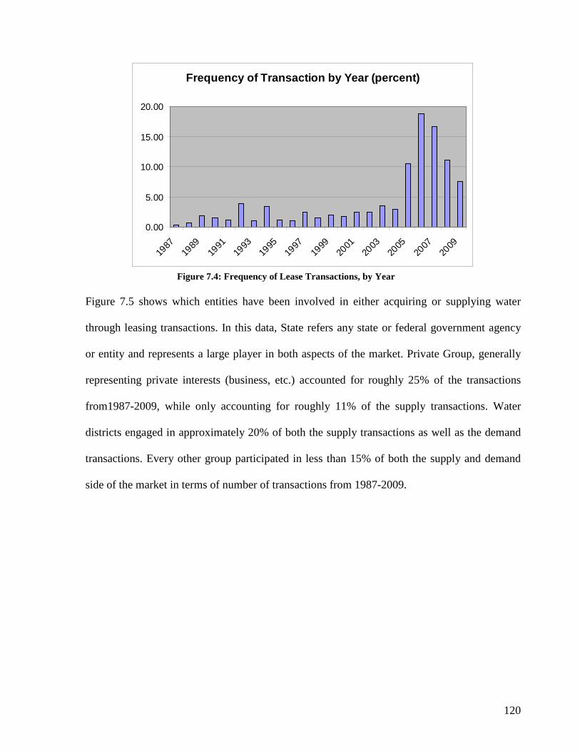
120

Frequency of Transaction by Year (percent)

0.00

5.00

10.00

15.00

20.00

1987

1989

1991

1993

1995

1997

1999

2001

2003

2005

2007

2009

Figure 7.4: Frequency of Lease Transactions, by Year

Figure 7.5 shows which entities have been involved in either acquiring or supplying water

through leasing transactions. In this data, State refers any state or federal government agency

or entity and represents a large player in both aspects of the market. Private Group, generally

representing private interests (business, etc.) accounted for roughly 25% of the transactions

from1987-2009, while only accounting for roughly 11% of the supply transactions. Water

districts engaged in approximately 20% of both the supply transactions as well as the demand

transactions. Every other group participated in less than 15% of both the supply and demand

side of the market in terms of number of transactions from 1987-2009.

121

Transactions (percent)

0

5

10

15

20

25

30

35

NGO Utility Ag Other WaterDist

PrivateGroup

State

AcquiredSupplied

Figure 7.5: Entities Supplying and Acquiring Water, by Percent

Figure 7.6 and 7.7 present the relative proportion the old use for each entitlement and the new

use for each lease, respectively. In both cases, the category “Other” represents at least 33% of

the total number of transactions. Other is comprised of the sum of transactions that comprise

less than 5% of the total market and transactions where the old use (or new use) is unknown.

The ambiguity is interesting because it may mean that there are many old and new uses and are

thus difficult to categorize and/or the documentation of old and new uses is not particularly

good so it is difficult to obtain a clear understanding of what exactly is occurring.

In figure 7.6, storage is a noteworthy old use because it is used as a regressor in the

econometric analysis while the other variables are not. Therefore, the hypothesis that storage as

the old use of the water is significantly different from other old uses. Additional old uses are

included in the chart to provide a visual assessment of the relative proportion of alternatives.

122

Old UseMunicipal

5%

Surplus5%

Storage19%

Ag20%

Other20%

Unknown31%

Figure 7.6: Proportion of Old Use

Three variables are noteworthy for the new uses in figure 7.7: municipal, which represents new

municipal use; environment, which represents new environmental use; and interstate compact,

which represents interstate compact being the new use. All three variables are used as

regressors in the econometric analysis. Agricultural new use and other new use are included in

the chart to provide perspective as to the relative proportions in the data.

New Use

Interstate Compact

1%Environment

12%

Ag13%

Municipal13%

Other61%

Figure 7.7: Proportion of New Use

123

7.2.2 Median Home Price Data

Figures 7.8, 7.9 and 7.10 present yearly median statewide home prices in both nominal dollars

and also adjusted for inflation to 2010 dollars for California, Colorado and New Mexico,

respectively. California values were provided by the California Association of Realtors.

Colorado values were provided by the National Association of Realtors and represent a

weighted average of Denver (80%) and Colorado Springs (20%) values, based roughly on

population. New Mexico values, also reported by the National Association of Realtors, use

Albuquerque values. In all cases, the year 2007 represents the beginning of a drop in home

prices, which coincides with start of the financial crisis. The starkest drop in price occurred in

California and has continued to fall in both California and Colorado. New Mexico prices, on

the other hand, have apparently begun to move upwards. It is unclear, however, whether the

New Mexico 2009 prices merely represent a data anomaly, a significant trend upwards or a

measurement error. Notice that the scale on the vertical axis is different for each figure.

California Median Home Prices

0

100000

200000

300000

400000

500000

600000

700000

1987

1989

1991

1993

1995

1997

1999

2001

2003

2005

2007

2009

medianadjusted (2010)

Figure 7.8: Median Home Price, California

124

CO Median Home Prices

0

50000

100000

150000

200000

250000

300000

1987

1989

1991

1993

1995

1997

1999

2001

2003

2005

2007

2009

Year

MedianAdjusted (2010)

Figure 7.9: Median Home Prices, Colorado

NM Median Home Prices

0

50000

100000

150000

200000

250000

1987

1989

1991

1993

1995

1997

1999

2001

2003

2005

2007

2009

Year

MedianAdjusted (2010)

Figure 7.10: Median Home Prices, New Mexico

125

5.2.3 Precipitation Data

Figure 7.11 shows monthly precipitation in inches by state beginning January 1986. The sharp

spikes indicate that California exhibits a high degree of volatility. Colorado and New Mexico

exhibit relatively less volatility. This measure is used as a proxy to represent relatively short-

term shortage or surplus.

Monthly Precipitation (inches)

0

2

4

6

8

10

12

14

1 25 49 73 97 121 145 169 193 217 241 265

Month (Beginning January 1986)

CACONM

Figure 7.11: Monthly Precipitation, by State

Figure 7.12 presents absolute statewide precipitation data in inches for California, Colorado

and New Mexico on an annual basis. On average, precipitation levels tend to be higher in

California; however, they appear more volatile. This measure is used to dull the impacts of

relatively short-term surplus or shortage and to help emphasize longer term variation.

126

Absolute Precipitation

0

5

10

15

20

25

30

35

40

1986

1988

1990

1992

1994

1996

1998

2000

2002

2004

2006

2008

year

prec

ipita

tion

(inch

es)

CACONM

Figure 7.12: Annual Precipitation

7.2.4 Temperature Data

Figure 7.13 shows monthly mean temperature by state. The figure shows the cyclical pattern of

increasing mid-year temperatures followed by falling end-of-year temperatures. Colorado

temperatures show significant inter-annual temperature variation, with relatively less

variability for New Mexico and even less for California.

127

Temperature (Farenheit)

0102030405060708090

1 25 49 73 97 121 145 169 193 217 241 265

Months (Beginning January 1986)

CACONM

Figure 7.13: Monthly Mean Temperature, by State

7.2.5 Climate Variables

Figure 7.14 shows data from three major climate indices, Multivariate ENSO Index (MEI),

Pacific Decadal Oscillation (PDO) and Atlantic Multidecadal Oscillation (AMO). Because

MEI, PDO and AMO are all climate variables, and should thus be measuring similar

phenomena, it is important to consider wither the indices are correlated. Tables 7.2 and 7.3

show the Pearson and Spearman correlation coefficients, respectively. In those tables, *

represents significance at a 10% level. The tables show that PDO and MEI are slightly

correlated as well as AMO and MEI; however, all variables were initially retained because the

correlation coefficient is not unacceptably large. PDO and AMO, however, show no significant

correlation. Because the econometric models used in this study utilized a lagged version of

PDO, the table below reports the correlation of the lagged variables. MEI was ultimately

dropped from the analysis because its use proved insignificant in preliminary modeling.

128

Climate Variability

-3

-2

-1

0

1

2

3

4

1 25 49 73 97 121 145 169 193 217 241 265

Months (Beginning Jan 1986)

MEIPDOAMO

Figure 7.14: Climate Variable Indicators

Pearson Correlation Coefficients,

N = 793

Spearman Correlation Coefficients, N = 793

Prob > |r| under H0: Rho=0

Prob > |r| under H0: Rho=0

PDO6lag MEI AMO6lag

PDO6lag MEI AMO6lag

PDO6lag 1.00

PDO6lag 1.00

MEI 0.23* 1.00 MEI 0.23*

AMO6lag -0.03 -0.37* 1.00 AMO6lag 0.06* -0.31* 1.00

Table 7.2: Pearson Correlation Coefficients Table 7.3: Spearman Correlation Coefficients 7.2.6 Population and Income

Figures 7.15 and 7.16 shows annual change in population and annual income, respectively.

Each graph begins from January 1987 and runs through December 2009. Total population is

almost always increasing in every year except for in Colorado in 2008, where it decreased.

Population change was used in this study rather than total population because it exhibits a

higher level of annual variability.

129

Change in Population

-0.05

-0.04

-0.03

-0.02

-0.01

0

0.01

0.02

0.03

0.04

0.05

1987

1989

1989

1991

1993

1995

1997

1999

2001

2003

2005

2007

2009

CaliforniaColoradoNew Mexico

Figure 7.15: Annual Population Change, by State

The graph below shows annual statewide mean personal income by quarter beginning January

1987. The general trend is for income to increase throughout each series; however, income

does decline beginning in 2008, coinciding with the financial market crisis.

Annual Personal Income (2010 Values)

0

50000

100000

150000

200000

250000

1 25 49 73

CaliforniaColoradoNew Mexico

Figure 7.16: Annual Personal Income, by State

130

7.2.7 Lake Mead Elevation

Figure 7.17 below shows the percent change in Lake Mead elevation levels, by month,

beginning January 1987. The graph shows a relatively large degree of monthly and annual

variability. Percent change was used in this analysis because it exhibited a higher degree of

variability than raw elevation levels.

Lake Mead Change in Elevation

-0.008

-0.006

-0.004

-0.002

0

0.002

0.004

0.006

0.008

1 49 97 145 193 241Change in Elevation

Figure 7.17: Lake Mead Elevation Change

7.3 Econometric Model - Introduction

In this study, I estimate demand models for lease prices in the states of California, Colorado

and New Mexico. Four models are considered: the Three State Model, which is a model

containing all of the data with state dummy variables; the California Model, a model only

containing data from the state of California; the Colorado Model, a model only containing data

from the state of Colorado; and the New Mexico Model, which only contains data from the

state of New Mexico.

131

Price is used as the dependent variable for several reasons. First, because the volume of

water in a particular region is essentially fixed when the transaction occurs, and is unlikely to

significantly change in the near future, price is relatively more responsive to changed

conditions and is more likely to be the mechanism to align supply and demand. Second,

determinants of price may be more relevant than determinants of quantity for policymaking

purposes. In order to analyze the opportunity cost of water, it is helpful to utilize a tool that

predicts price and adjust those determinants, such that private water values, which more closely

coincide with social values.

Because price and quantity are presumed to be simultaneously determined in a demand

function, it is necessary to consider whether price and quantity are endogenous. To conduct

this analysis, it is important to utilize variables for which strong instruments exist and

instruments for quantity tend to be stronger than for price (Jones 2008). Weak instruments may

lead to biased results and incorrect asymptotic properties, even in large samples (Staiger and

Stock 1997). For these reasons, an instrumented quantity is determined thereby leaving price as

the choice dependent variable. The instruments include all the demand equation variables

(excluding quantity) plus additional exogenous variables. The exogenous variables are

included to ensure the instruments chosen are at least partially correlated with quantity after

controlling for the effect of the other variables (Wooldridge 2002). Finally, as previously

mentioned, the logarithm of price is used (LNDOLPERAFADJ) because it returns errors that

are more normally distributed than an untransformed price is used.

In a first exploratory model, price is regressed on quantity using ordinary least squares.

In order for the model to behave normally, the parameter for quantity should be decreasing.

That is, the marginal effect of quantity on price should be negative.

132

Parameter Estimates Variable Parameter

Estimate Standard Error

t Value Pr > |t|

Intercept 200.88 12.3 16.33 <.0001 Quant -9.24E-7 1.64E-6 -0.56 0.5746

Table 7.4: Univariate Regression Results; Price Regressed on Quantity The SAS output shows an insignificant negative parameter for quantity; however, the marginal

effect of quantity on price may still negative when the Three State Model is considered or

when individual state models are examined.

Endogeneity between price and quantity was then tested using the regression form of

the Hausman test (Wooldridge 2002). The regression endogeneity test consists of an initial

regression using ordinary least squares. Quantity is regressed on the proposed instruments and

the residuals are saved. Price is then regressed on quantity, the exogenous variables, and the

residuals also using ordinary least squares. A significant parameter for the predicted errors

suggests the errors from quantity are related to the errors of the price equation and are therefore

endogenous (Jones 2008). The output below shows parameter estimates and significance of the

key variable QUANTRESIDUAL, which is the parameter associated with the predicted errors.

The table includes the entire sample and output for each state.

Entire Sample California Colorado New Mexico quantresidual 1.03E-5 -8.02E-6 -1.04E-5 7.42E-6 t-statistic -0.99 -0.82 -0.57 0.64 p-value 0.32 0.41 0.57 0.52

Table 7.5: Test of Endogeneity, Results

For the entire sample, California, Colorado, and New Mexico, endogeneity was not detected.

However, heteroskedasticity was detected using the Breusch-Pagan test (Johnston and DiNardo

1996) so the above results were then adjusted utilizing White’s Robust Standard Errors. This

was done by inserting /ACOV after the model statement in SAS.

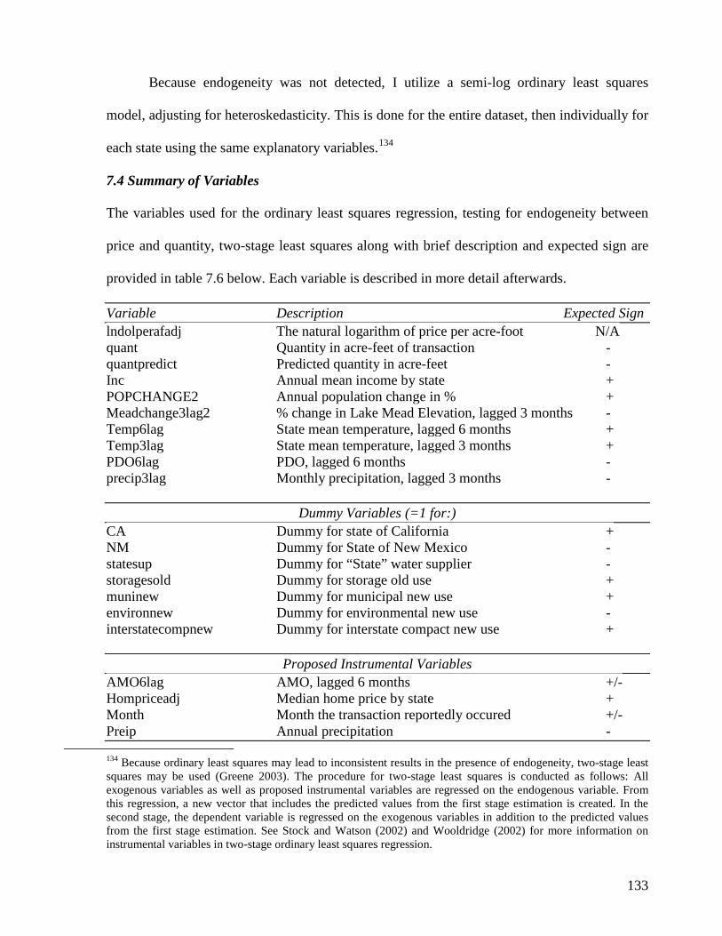
133

Because endogeneity was not detected, I utilize a semi-log ordinary least squares

model, adjusting for heteroskedasticity. This is done for the entire dataset, then individually for

each state using the same explanatory variables.134

7.4 Summary of Variables

The variables used for the ordinary least squares regression, testing for endogeneity between

price and quantity, two-stage least squares along with brief description and expected sign are

provided in table 7.6 below. Each variable is described in more detail afterwards.

Variable Description Expected Sign lndolperafadj The natural logarithm of price per acre-foot N/A quant Quantity in acre-feet of transaction - quantpredict Predicted quantity in acre-feet - Inc Annual mean income by state + POPCHANGE2 Annual population change in % + Meadchange3lag2 % change in Lake Mead Elevation, lagged 3 months - Temp6lag State mean temperature, lagged 6 months + Temp3lag State mean temperature, lagged 3 months + PDO6lag PDO, lagged 6 months - precip3lag Monthly precipitation, lagged 3 months -

Dummy Variables (=1 for:) CA Dummy for state of California + NM Dummy for State of New Mexico - statesup Dummy for “State” water supplier - storagesold Dummy for storage old use + muninew Dummy for municipal new use + environnew Dummy for environmental new use - interstatecompnew Dummy for interstate compact new use +

Proposed Instrumental Variables AMO6lag AMO, lagged 6 months +/- Hompriceadj Median home price by state + Month Month the transaction reportedly occured +/- Preip Annual precipitation -

134 Because ordinary least squares may lead to inconsistent results in the presence of endogeneity, two-stage least squares may be used (Greene 2003). The procedure for two-stage least squares is conducted as follows: All exogenous variables as well as proposed instrumental variables are regressed on the endogenous variable. From this regression, a new vector that includes the predicted values from the first stage estimation is created. In the second stage, the dependent variable is regressed on the exogenous variables in addition to the predicted values from the first stage estimation. See Stock and Watson (2002) and Wooldridge (2002) for more information on instrumental variables in two-stage ordinary least squares regression.

134

Quantresidual Residuals when quantity regressed on Instruments +/- Table 7.6: Variables, Descriptions and Expected Signs

Description of Variables and Expected Signs:

LNDOLPERAFADJ: is the natural logarithm of price per acre-foot for each lease

transactions. Price was deflated to January 2010 prices. Price is the dependent variable.

QUANT: is the actual quantity associated with each lease transaction. The quantity parameter

is expected to be negative as the functional form for a demand equation is used.

QUANTPREDICT: is the predicted quantity obtained from the first stage of the two-stage

least squares estimation. Like actual quantity, this parameter is expected to be negative.

QUANTRESIDUAL: is a vector of residuals obtained from regressing quantity on the

proposed instruments. This variable is obtained for the purpose of testing for endogeneity

between price and quantity.

INC: Mean annual income by state in January 2010 prices. This parameter is expected to be

positive. As income increases, the price that individuals are willing to pay should also increase.

POPCHANGE2: is the annual change in population for each state reported in percent terms.

This parameter is expected to be positive because as population grows, we expect greater strain

and a higher level of demand on the resource.

MEADCHANGE3LAG2: is the monthly change in Lake Mead elevation in percentage terms,

lagged three months. This parameter is expected to be negative because as elevation level

increases, we expect the supply of available water to also increase, leading to a decrease in

price.

TEMP: is the mean monthly temperature by state. This parameter is expected to be positive

because as temperature increases, demand is expected to simultaneously increase.

135

PDO#LAG: represents the value of the Pacific Decadal Oscillation index, lagged # months.

This parameter is expected to be negative. As PDO increases, winter La Nina conditions are

expected to be muted, thereby making it more likely that precipitation will occur in those

months and increasing water availability.

AMO#LAG: represents the Atlantic Multidecadal Oscillation index lagged # months. It is

unknown whether this parameter is positive or negative.

PRECIP#LAG: is the monthly precipitation by state lagged # months. This parameter is

expected to be negative. As rainfall increases we expect that price will decrease.

PRECIP: is the annual precipitation. This parameter is expected to be negative. Greater

availability of water should lead to lower prices.

HOMPRICEADJ: is the annual median home sales price by state adjusted to January 2010

prices. It is unclear whether this parameter will be positive or negative.

CA: is the dummy variable representing the state of California. This parameter is expected be

positive as the highest demand pressures for water appear to currently be in California.

NM: is the dummy variable representing New Mexico. This parameter is expected to be

negative because the demand pressures for water appear to be relatively lower in New Mexico.

STATESUP: is the dummy variable representing the state as a supplier of water to the market.

Here, state represents federal, state and city suppliers. This parameter is expected to be

negative as the state is more likely to subsidize water transactions thereby artificially reducing

the price.

STORAGESOLD: is the dummy variable representing storage being the old use of the water.

This parameter is expected to be positive because we expect relatively high costs of recovering

the water from storage facilities.

136

MUNINEW: is the dummy variable representing the new use of the water being municipal.

This parameter is expected to be positive as a municipality is likely to acquire water in the

event of an emergency or when available supplies are low.

ENVIRONNEW: is the dummy variable representing environmental use being the new use of

the water. Consistent with Jones (2007), this parameter is expected to be negative.

Environmental use is expected to be subsidized, leading to a lower price.

INTERSTATECOMPNEW: is the dummy variable representing the satisfaction of an

interstate compact being the new use of the water. This parameter is expected to be positive as

states will be willing to spend a relatively high amount to ensure that interstate compacts are

not violated.

137

8. RESULTS and ANALYSIS

Four models are used in this study: Three State model, California model, Colorado model and

New Mexico model. The Three State model is a compilation of data from the California,

Colorado and New Mexico models where Colorado is the excluded dummy variable. After a

methodological introduction, raw results from SAS are provided. Following the raw results is a

discussion of the marginal effects of each model as well as an interpretation of results.

8.1 Econometric Results

Where practicable, all four models utilize the same variables. A major exception is that the

Three State model and the California model use the temperature lagged 6 months variable

(TEMP6LAG), while the Colorado and New Mexico models use the temperature lagged 3

months variable (TEMP3LAG). This was done because preliminary results suggested that

Colorado and New Mexico prices were more responsive to a 3-month lag, while California

prices were more responsive to a 6-month lag. Because the majority of observations in the

Three State model are from California, it was determined that a 6-month lag is appropriate in

that model. In the individual state models, some variables were deleted to ensure that the

models were not over-specified and full rank. For instance, the state dummy variables were

deleted in all of the individual state models. Additionally, INTERSTATCOMPNEW was

deleted from the California model and MUNINEW was deleted from the New Mexico model

as the Water Strategist did not report that that either state had engaged in those respective types

of leasing transactions over the time period studied.

All models are in a semi-log form. Non-dummy variable parameters represent the

percent change in price for a one-unit increase of that particular variable. The marginal effect

of dummy variables, on the other hand, are calculated by raising the exponential function to the

value of the reported parameter and subtracting by one (Kennedy 2003).

138

8.1.1 Three States Model Results

Below are regression results from the ordinary least squares regression of the entire sample,

adjusted for heteroskedasticity.

Analysis of Variance Source DF Sum of Mean F

Value Pr > F

Squares Square

Model 14 214.29 15.31 10.93 <.0001 Error 777 1089.69 1.40 Corrected Total

791 1303.98

Root MSE 1.18 R-Square 0.16 Dependent Mean

4.49 Adj R-Sq 0.15

Coeff Var 26.34

Parameter Estimates Variable Parameter Robust Standard

Errors Estimate Standard t Value Pr > |t|

Error Intercept 5.77 0.51 11.30 <.0001

CA -0.06 0.18 -0.33 0.74 NM -0.62 0.35 -1.77 0.08 Inc -2.4E-6 2.3E-6 -1.05 0.29 Popchange2 -0.03 0.03 -0.90 0.37

Meadchange3lag2 1.12 0.26 4.29 <.0001 Temp6lag -.005 0.0004 -0.67 0.51

PDO6LAG 0.19 0.05 4.24 <.0001

precip3lag -0.15 0.03 -5.97 <.0001

Statesup -0.55 0.11 -4.88 <.0001

Storagesold 0.32 0.12 2.62 0.009

139

Muninew -0.37 0.11 -3.26 0.001

Environnew -0.90 0.21 -7.25 <.0001

interstatecompnew -1.67 0.21 -7.80 <.0001

Quant 1.4E-6 1.3E-6 1.05 0.30 Table 8.1: Regression Results, Entire Sample

8.1.2 California Model Results

Below are regression results from the ordinary least squares regression of the California

sample, adjusted for heteroskedasticity.


Value Pr > F

Squares Square


500 774.69

Root MSE 1.14 R-Square 0.17

Dependent Mean

4.55 Adj R-Sq 0.15

Coeff Var 25.21



Error Intercept 5.57 0.62 8.92 <.0001 Inc 1.2E-6 3E-6 0.39 0.70 Popchange2 0.04 0.01 0.46 0.65 Meadchange3lag2 1.75 0.32 5.32 <.0001 Temp6lag -0.01 0.006 -2.20 0.03

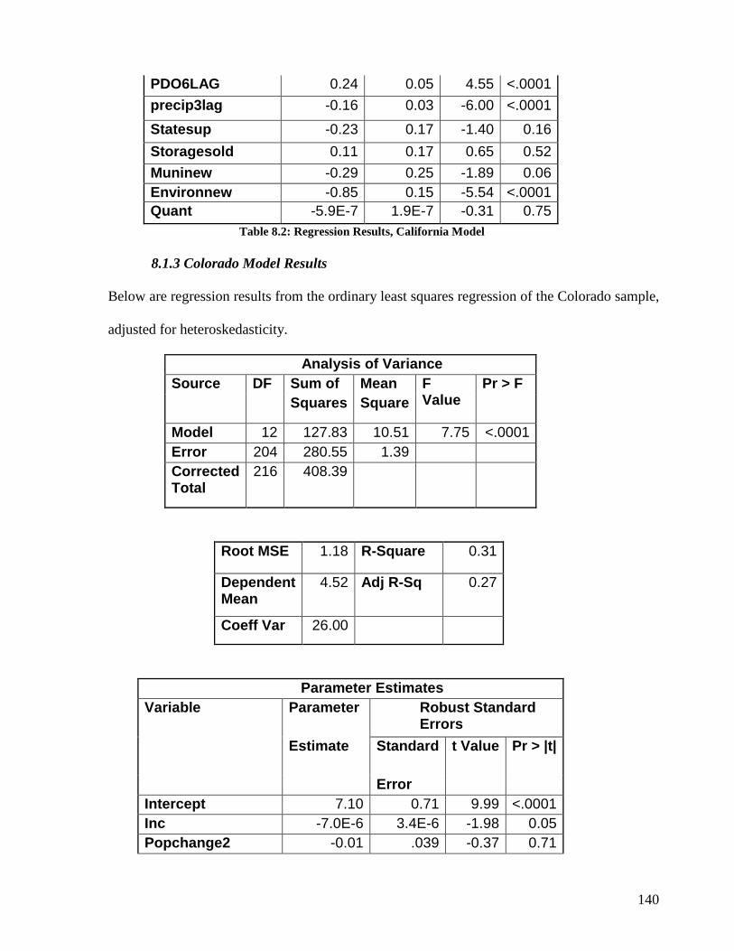
140

PDO6LAG 0.24 0.05 4.55 <.0001 precip3lag -0.16 0.03 -6.00 <.0001

Statesup -0.23 0.17 -1.40 0.16 Storagesold 0.11 0.17 0.65 0.52 Muninew -0.29 0.25 -1.89 0.06 Environnew -0.85 0.15 -5.54 <.0001 Quant -5.9E-7 1.9E-7 -0.31 0.75

Table 8.2: Regression Results, California Model

8.1.3 Colorado Model Results

Below are regression results from the ordinary least squares regression of the Colorado sample,

adjusted for heteroskedasticity.


Value Pr > F

Squares Square


216 408.39

Root MSE 1.18 R-Square 0.31

Dependent Mean

4.52 Adj R-Sq 0.27

Coeff Var 26.00



Error Intercept 7.10 0.71 9.99 <.0001 Inc -7.0E-6 3.4E-6 -1.98 0.05 Popchange2 -0.01 .039 -0.37 0.71

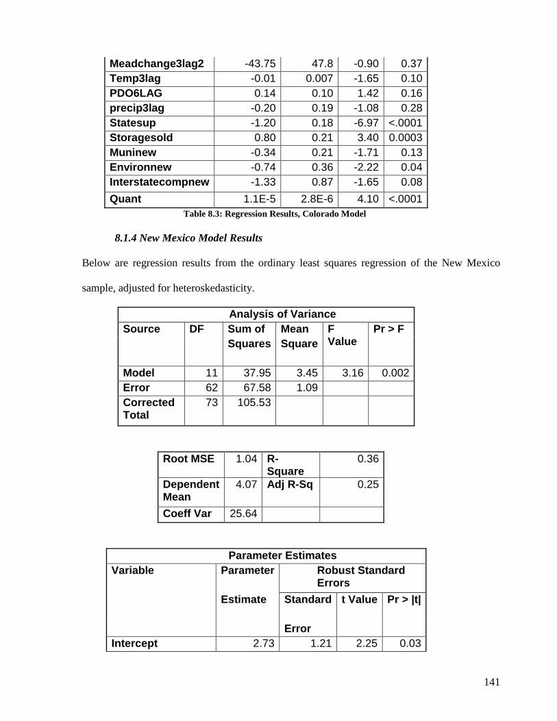
141

Table 8.3: Regression Results, Colorado Model

8.1.4 New Mexico Model Results

Below are regression results from the ordinary least squares regression of the New Mexico

sample, adjusted for heteroskedasticity.


Value Pr > F

Squares Square

Model 11 37.95 3.45 3.16 0.002 Error 62 67.58 1.09 Corrected Total

73 105.53

Root MSE 1.04 R-Square

0.36

Dependent Mean

4.07 Adj R-Sq 0.25

Coeff Var 25.64



Error Intercept 2.73 1.21 2.25 0.03

Meadchange3lag2 -43.75 47.8 -0.90 0.37 Temp3lag -0.01 0.007 -1.65 0.10 PDO6LAG 0.14 0.10 1.42 0.16 precip3lag -0.20 0.19 -1.08 0.28 Statesup -1.20 0.18 -6.97 <.0001 Storagesold 0.80 0.21 3.40 0.0003 Muninew -0.34 0.21 -1.71 0.13 Environnew -0.74 0.36 -2.22 0.04 Interstatecompnew -1.33 0.87 -1.65 0.08 Quant 1.1E-5 2.8E-6 4.10 <.0001

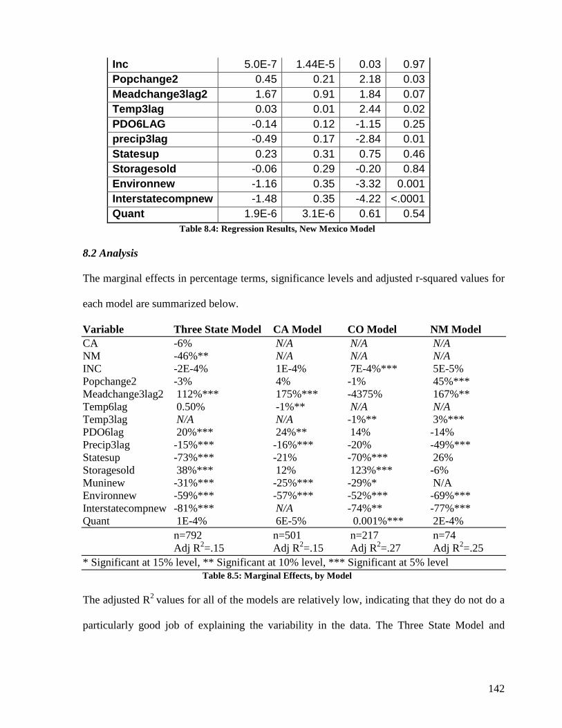
142

Inc 5.0E-7 1.44E-5 0.03 0.97 Popchange2 0.45 0.21 2.18 0.03 Meadchange3lag2 1.67 0.91 1.84 0.07 Temp3lag 0.03 0.01 2.44 0.02 PDO6LAG -0.14 0.12 -1.15 0.25 precip3lag -0.49 0.17 -2.84 0.01 Statesup 0.23 0.31 0.75 0.46 Storagesold -0.06 0.29 -0.20 0.84 Environnew -1.16 0.35 -3.32 0.001 Interstatecompnew -1.48 0.35 -4.22 <.0001 Quant 1.9E-6 3.1E-6 0.61 0.54

Table 8.4: Regression Results, New Mexico Model

8.2 Analysis

The marginal effects in percentage terms, significance levels and adjusted r-squared values for

each model are summarized below.

Variable Three State Model CA Model CO Model NM Model CA -6% N/A N/A N/A NM -46%** N/A N/A N/A INC -2E-4% 1E-4% 7E-4%*** 5E-5% Popchange2 -3% 4% -1% 45%*** Meadchange3lag2 112%*** 175%*** -4375% 167%** Temp6lag 0.50% -1%** N/A N/A Temp3lag N/A N/A -1%** 3%*** PDO6lag 20%*** 24%** 14% -14% Precip3lag -15%*** -16%*** -20% -49%*** Statesup -73%*** -21% -70%*** 26% Storagesold 38%*** 12% 123%*** -6% Muninew -31%*** -25%*** -29%* N/A Environnew -59%*** -57%*** -52%*** -69%*** Interstatecompnew -81%*** N/A -74%** -77%*** Quant 1E-4% 6E-5% 0.001%*** 2E-4% n=792 n=501 n=217 n=74 Adj R2=.15 Adj R2=.15 Adj R2=.27 Adj R2=.25 * Significant at 15% level, ** Significant at 10% level, *** Significant at 5% level

Table 8.5: Marginal Effects, by Model

The adjusted R2 values for all of the models are relatively low, indicating that they do not do a

particularly good job of explaining the variability in the data. The Three State Model and

143

California model are particularly poor with an adjusted R2 of only .15. The Colorado and New

Mexico models provide relatively better results with an adjusted R2 of .27 and .25, respectively.

For the purpose of comparison, the adjusted R2 in Jones (2008) ranged from .32 to .45

when lease prices were modeled, depending on model. In that study, Arizona, New Mexico,

Utah and California were modeled together in a two-stage least squares procedure. Also

modeling lease prices, Pittenger (2005) found an adjusted R2 ranging from .30 to .74,

depending on which model was used. In that study, Arizona, California, Colorado, Idaho, New

Mexico, Oregon and Texas were modeled separately. Additional models combining states by

region were also tested with similar results. Two-stage least squares was used for models

where endogeneity was present, while ordinary least squares was used when it was not. In both

previous studies, the results show an improved adjusted R2 when compared to the adjusted R2

in the present study. A likely culprit for the relatively lower values is the statewide spatial scale

used; both Jones (2008) and Pittenger (2005) use a spatial scale of climate division. As a result,

those models are more likely to pick up the intrastate climate and demographic variation,

whereas an analysis based upon a statewide spatial scale is blind to that variation.

The variable, QUANT, which is the quantity figure in acre-feet for each transaction, is

insignificant in every model except for the Colorado model. The models in which quantity is

insignificant likely indicate that quantity does not have a significant impact on price. This is

not necessarily a surprise because when price was regressed on quantity in the univariate case,

it was not significant. In the Colorado model, the quantity is positive and indicates that a 1

acre-foot increase in quantity leads to a price increase of 0.001%. The increasing relationship is

counter to assumption that the phenomenon being modeled is a downward sloping demand

curve (downward sloping in quantity). This may be explained by the possibility that

transactions with higher quantities tend to have more impediments to transfer, and thus have

144

higher transactions costs. Nevertheless, the overall results suggest that quantity and price are

only tenuously related in water lease transactions. And if they are related at all, a positive

relationship seems to exist. Jones (2008) found a similar result; in her non-environmental lease

estimation, the quantity parameter was positive and (barely) significant, in her environmental

lease estimation, it was insignificant. Pittenger (2005) also showed mixed results. In the

California model, the quantity parameter was insignificant while the quantity parameter in the

New Mexico model was positive and significant. It is important to note, however, that the

results are not strictly comparable because Jones (2008) and Pittenger (2005) utilized two-stage

least squares for the models discussed.

The dummy variables for the states of California and New Mexico are only present in

the Three State Model. The New Mexico dummy is significant and negative. The marginal

effect of -46% indicates that lease prices are 46% lower in New Mexico than the other states.

The California dummy is insignificant in the model. Because Colorado is the base state, the

insignificant California dummy implies that there is no significant difference in price between

California and Colorado. This is consistent with the analysis of the dependent variables already

undertaken that found that the prices in California and Colorado were not statistically different

from each other but were both different from New Mexico.

INC, the variable for annual personal income by state, is only significant in the

Colorado model. The income variable for that state is positive and marginal effect indicates

that a one dollar increase in annual income leads to a 0.007% in price. The positive nature of

this variable was expected; as income increases, price was expected to increase. The

insignificance of income in the Three State Model, the California model and the New Mexico

model indicates that annual personal income does not have a significant on price in those

models. Jones (2008) found income to be significant in both her environmental lease model as

145

well as her non-environmental lease model. In her environmental lease model, the parameter

was positive and small (.0001%) while in her non-environmental lease model, the marginal

effect was negative and small (-.0001%). Despite the mixed results with respect to sign, the

small value of the marginal effects in absolute terms suggests that income tends to have an

extremely small, albeit detectable, impact on lease prices.

POPCHANGE2, the variable indicating the percent change in state population, is only

significant in the New Mexico model. The marginal effect is positive and indicates that a one

percent increase in population in the state of New Mexico causes price to increase by 45%

percent. This is a rather large increase in price for a small percentage increase in population;

nevertheless, the result is not counterintuitive as the expected sign for this variable was

positive.

MEADCHANGE3LAG2, the variable representing the monthly change in Lake Mead

elevation by percent, lagged 3 months, is significant at a 5% level in the Three State Model and

the California model and significant at a 10% level in the New Mexico model. In all cases in

which this variable is significant, the result is initially counterintuitive. I expected that as Lake

Mead elevation increased price would decline as a larger supply of water would be available.

Nevertheless this result can reasonably be explained by considering the possibility that

increasing Lake Mead elevation is an administrative storage goal. One way to accomplish this

goal is to create impediments to transfer, thereby making the costs of transfer greater. The

marginal effect for the Three State Model is 112%, indicating that as Lake Mead elevation

increases by 1%, price also increases 112%. The marginal effect for the California model

indicates that a 1% increase in elevation leads to 175% price increase. A similar analysis can

be conducted for the state of New Mexico. The marginal effect indicates that a 1% increase in

elevation leads to a 167% increase in price. While these marginal values appear large, they are

146

moderated by the fact that the month-to-month variation is small. The data ranges from -.55%

to .65%, with a mean monthly change of -.03%. Additionally, approximately 68% of the data

ranges from -.21% to .15%. Therefore, when the relatively small decimal terms are multiplied

with the relative large marginal effects, the marginal impact on price is muffled.

TEMP6LAG, the variable representing state mean temperature lagged 6 months is

significant at a 10% level in the California model and insignificant in the Three State Model.

The Marginal effect is negative and indicates that a one degree increase in temperature leads to

a 1% decrease in price. The expected sign was for this variable was positive, so this result is

counter to what was expected. TEMP3LAG, the variable representing mean temperature

lagged 3 months is significant at a 10% level in the Colorado model and at a 5% level in the

New Mexico model. The marginal effect for the Colorado model in negative and, like the

California model indicates that a one degree temperature increase leads to a 1% increase in

price. Alternatively, the marginal effect for the New Mexico model is positive and indicates

that a one degree increase in temperature leads to a 3% increase in price. It is unclear why

California and Colorado have unexpected negative marginal effects, while New Mexico has an

expected positive marginal effect. In general, Jones (2008) found temperature to be

insignificant or only slightly significant, which is contrary to the results in this study, which

found temperature to be significant.

PDO6LAG, the variable representing the Pacific Decadal Oscillation index, lagged 6

months, is significant in the Three State Model at a 5% level and the California model at a 10%

level. It is insignificant in the Colorado and New Mexico models. The marginal effect of the

Three State Model is 20% indicating that a one unit change in PDO, 6 months in advance,

leads to a 20% increase in price. The marginal effect for the California model is 24% indicating

that price increases 24% when PDO increases by one unit, 6 months in advance. The expected

147

parameter for this variable was negative, so the result is counter to the expectation. It is unclear

why the actual parameter is positive; however, there are two likely explanations for this. First,

the impact of PDO on water supply availability may be poorly understood and therefore the

expectation of lower prices when PDO increases may not be correct. Second, because this

variable was lagged 6 months, the lag has not been properly accounted for. The insignificance

of PDO in the Colorado and New Mexico models suggests that it does not play a significant

role in the prices in those states. Nevertheless, prior studies suggest that PDO does play a role

in New Mexico and Colorado precipitation patterns. Brown and Comrie (2002) found that

PDO exhibits a strong relationship with winter and spring precipitation in New Mexico, while

Schoennagel et al (2005) found that PDO variability impacts precipitation in Colorado. As

such, more research is required to untangle the relationship between PDO, precipitation and

lease prices in Colorado and New Mexico.

The variable for precipitation, PRECIP3LAG, which is the monthly precipitation by

state, lagged 3 months, is significant in all of the models at a 5% level of significance except

for the Colorado Model. As expected, in all of the models in which the precipitation variable is

significant the parameter is negative. In the Three State Model the marginal effect of 15%

indicates that a one inch increase in rainfall leads to a price decrease of 15%. In the California

model, the marginal effect indicates that one inch of precipitation leads to a decrease in price of

16%. The most extreme case is in the New Mexico model, where one inch of precipitation

leads to a price decrease of 49%. The expected sign of this variable was negative as it was

assumed that because precipitation brings about greater water supply availability, the price

should decline. Although a slightly different variable was used in Jones (2008) and Pittenger

(2005), both found precipitation to be significant with a negative marginal effect. This uniform

148

result provides important evidence of the relationship between the inverse relationship between

precipitation and the demand for water.

STATESUP, the dummy variable for state supplier is negative and significant at a 5%

level of significance only in the Three State Model and the Colorado model. Recall that state

suppliers refers to any water lease transaction where the supplier is a city, the respective state

or a federal supplier. For the Three State Model, a negative marginal effect of 73% indicates

that leases that are supplied by a state entity are lower than other leases supplied by other

entities by 73%. Likewise, the marginal effect of -70% for the Colorado model indicates that

state suppliers provide a 70% discount. The negative marginal effect was expected as I

assumed that when the state supplies water it would do so at a discount. The fact that the

parameter is insignificant for the Colorado and New Mexico models indicates that the price of

leases by state suppliers is not significantly different from other suppliers.

STORAGESOLD, the dummy variable representing the old use of the water being in

storage is positive and only significant in the Three State Model and the Colorado model. The

marginal effect of the Three State Model is 38%, indicating that water coming out of storage is

38% more expensive that water obtained from other means. The Colorado marginal effect is

also positive and rather large. The marginal effect indicates that water coming out of storage is

123% more expensive that other old uses. This result coincides with the expected positive sign.

It was expected that water obtained from storage has costly administrative impediments to

transfer; thus the marginal effect should be positive. The insignificant parameters for the

California and New Mexico models indicate that water obtained from storage is not statistically

different in price from water obtained from other old uses.

MUNINEW, the dummy variable representing new municipal use, is negative and

significant at a 5% level in the Three State Model and the California model, negative and

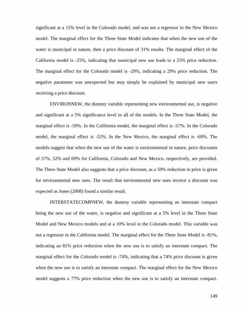
149

significant at a 15% level in the Colorado model, and was not a regressor in the New Mexico

model. The marginal effect for the Three State Model indicates that when the new use of the

water is municipal in nature, then a price discount of 31% results. The marginal effect of the

California model is -25%, indicating that municipal new use leads to a 25% price reduction.

The marginal effect for the Colorado model is -29%, indicating a 29% price reduction. The

negative parameter was unexpected but may simply be explained by municipal new users

receiving a price discount.

ENVIRONNEW, the dummy variable representing new environmental use, is negative

and significant at a 5% significance level in all of the models. In the Three State Model, the

marginal effect is -59%. In the California model, the marginal effect is -57%. In the Colorado

model, the marginal effect is -52%. In the New Mexico, the marginal effect is -69%. The

models suggest that when the new use of the water is environmental in nature, price discounts

of 57%, 52% and 69% for California, Colorado and New Mexico, respectively, are provided.

The Three State Model also suggests that a price discount, as a 59% reduction in price is given

for environmental new uses. The result that environmental new uses receive a discount was

expected as Jones (2008) found a similar result.

INTERSTATECOMPNEW, the dummy variable representing an interstate compact

being the new use of the water, is negative and significant at a 5% level in the Three State

Model and New Mexico models and at a 10% level in the Colorado model. This variable was

not a regressor in the California model. The marginal effect for the Three State Model is -81%,

indicating an 81% price reduction when the new use is to satisfy an interstate compact. The

marginal effect for the Colorado model is -74%, indicating that a 74% price discount is given

when the new use is to satisfy an interstate compact. The marginal effect for the New Mexico

model suggests a 77% price reduction when the new use is to satisfy an interstate compact.

150

This result was unexpected as I had assumed that the satisfaction of an interstate compact

would require the party seeking to satisfy the compact to transfer water on short notice, thereby

having to pay a premium. Nevertheless, the negative result indicates that the party receives a

discount.

8.3 Interpretation of Results

The four models suggest that despite the fact that the same variables were used, each state is

idiosyncratic and different drivers cause price to change in each state. It is clear that prices in

California and Colorado are higher than in New Mexico, ceteris paribus, and that prices in

California and Colorado are not statistically different from each other. This conclusion is

drawn from the results of the difference of means test on the prices as well as the dummy

variable for the state of New Mexico being significant while California, and by implication

Colorado, is insignificant in the Three State Model.

Demographic variables, such as income and population, do not appear to have much

impact on price. The sole exception is New Mexico, which has a relatively large and positive

marginal impact of population on price. These variables may be largely insignificant because

the data tends to have relatively little variation and therefore does a poor job at explaining

dependent variable variation. This lack of variation can be attributed to two factors. First, the

data is either annual or quarterly and so for each model there are a relatively small number of

observations. Second, the data from one year to the next, or quarter to quarter, does not

significantly vary. Population is nearly always increasing but at a relatively slow rate.

Although the change in population, the variable used in this study, does display some

variability, it is almost always positive. Likewise, income tends to increase slowly and displays

very little variability.

151

The climate variable, PDO6LAG, and temperature and precipitation variables are

interesting because they are significant in some models and insignificant in others. Another

interesting factor is that while these variables may help to explain water lease prices, they

cannot be used in any way as policy tools to increase or decrease demand, as we do not have

the technological capability to alter those variables. Nevertheless, an understanding of the

manner in which these variables operate may provide some insight into price change as well as

provide a useful tool to assist in price forecasting and planning for future supplies. The PDO

variable is significant in the Three State Model and the California model and insignificant in

the others. This is somewhat surprising as PDO is believed to strongly impact both Colorado

and New Mexico. More study is necessary to assess the manner in which PDO impacts those

states. The temperature variables provide some significant results; however, the results are

often counterintuitive. Perhaps other noise in the models is creating the result. The

precipitation variable, on the other hand, is generally significant with the expected sign. It

appears that price properly declines concurrently with the water supply adjustment (increase).

The variable for the change in Lake Mead elevation is interesting because it may help

to provide insight into how price changes in the face of changing administrative and

operational regional water storage goals. That is, if it is the case that the goal is to increase

elevation levels, then as elevation increases the price should also increase. This is counter to

what was originally expected; however, this result is probably more interesting because a

detectable increase in price can be seen that coincides with the underlying policy goals. As a

result, individuals participating in the market can make informed decisions and policymakers

can have a better understanding of the overarching impact of their policy.

The dummy variable for state supplier is negative and significant only in the Three

State Model and the Colorado model. The dummy variable for storage being the old use is

152

positive and is also only significant in those two models. Both of these results can provide

important political and policy implications. First, because the state provides a price discount

when supplying water in Colorado, care must be used when it engages in a particular

transaction as those prices do not coincide with market values. Second, because water obtained

from storage tends to be priced higher, that can provide a strong disincentive to withdrawing

the water. If the goal of a particular program is to bank water for a later date, then the higher

price of stored water can ultimately assist in that effort.

The new use variables used in these models, municipal new use, environmental new use

and interstate compact new use are negative and significant in all of the models. All of the

models suggest that discounts are provided for these types of new uses; by implication, other

new users are required to pay a higher price. Nevertheless, this result should be used with

caution because it is unclear what the other new uses are. By construction, the base new use in

these models is not clearly defined and the new uses in these models only account for a small

percentage of transactions. As a result, more information can be gleaned about the particular

new uses in the models than the alternatives not included.

Finally, the quantity variable is interesting because, with the exception of the Colorado

model, it is insignificant. In the Colorado model, the variable is significant and positive, but

extremely small. Although the positive result in the Colorado case was not expected, it may be

explained by the possibility that larger quantity transactions have more impediments to

transfer, thus causing price to increase. Regardless of this result, it appears as though the

relationship between price and quantity in water lease transactions is tenuous and price is likely

driven by factors other than price.

153

9. NET RETURNS OVER VARIABLE COST and PILOT PROGRAMS

This chapter provides data and analysis for net returns over variable costs for four crops

produced in Yuma County, Arizona. Also provided is analysis of four pilot fallowing programs

that the US Bureau of Reclamation has recently entered into.

9.1 Yuma County NROVC

Net returns over variable cost (NROVC) provides a benchmark that is often used to represent

the minimum payment required for an irrigator to cease irrigation. To compute NROVC, the

variable costs of production are subtracted from the revenues obtained, on a per-acre basis.

Because the per-unit value of water is of interest in this study, the difference is divided by the

consumptive volume of water per-acre necessary for production of the particular crop. The

consumptive volume estimates used in this study were obtained from the Bureau of

Reclamation’s Final Environmental Impact Statement (BOR 2007). Crop prices and input costs

were updated to their current levels. Fertilizer, insecticide and herbicide prices were collected

through personal interviews with input suppliers. For a detailed summary, see Appendix C.

Tables 9.1, 9.2, 9.3 and 9.4 present data on net returns over variable cost per acre-foot

of water for Durum Wheat, Alfalfa, Upland Cotton and Head Lettuce, respectively, in Yuma

County, Arizona. With the exception of the Upland Cotton table, each contains a column

representing average values for the years 2002-2006, a column representing average values for

the years 2005-2009, and a column representing the change of those two averaged series in

percentage terms. The Upland Cotton table contains the average values for the years 2006-

2008 instead of 2005-2009 because a full set of data was not available for the relevant 5 year-

long comparison. In order to assess trends in the two time-periods, gross revenues per acre,

total variable costs per acre and net returns over variable costs per acre are also included in

each table. Figures in parentheses represent negative values.

154

Table 9.1: NROVC, Durum Wheat

Table 9.2: NROVC, Alfalfa

Table 9.3: NROVC, Upland Cotton

Table 9.4: NROVC, Head Lettuce

Yuma Durum Wheat 5yr Avg Year Range 2002-2006 2005-2009 % Change Gross Revenue ($/Acre) 455.94 710.25 55.78 Total Variable Costs per Acre 377.82 582.02 54.05 Net Returns Over Variable Costs per Acre

78.12

128.23

71.83

Net Returns Over Variable Costs Per Acre-foot of Water Consumed

41.12

67.49

64.13

Yuma Alfalfa 5yr Avg Year Range 2002-2006 2005-2009 % Change Gross Revenue ($/Acre) 1006.26 1329.05 32.08 Total Variable Costs per Acre 400.79 624.79 55.89 Net Returns Over Variable Costs per Acre

605.47

704.26

16.32


106.22

123.55

16.32

Yuma Upland Cotton 5yr and 3yr Avg Year 2002-2006 2006-2008 % Change Gross Revenue ($/Acre) 965.03 1063.87 10.24 Total Variable Costs per Acre 1150.33 1318.20 14.59 Net Returns Over Variable Costs per Acre

(185.30)

(254.33)

(37.25)


(51.47)

(70.65)

(37.26)

Yuma Head Lettuce 5yr Avg Year 2002-2006 2005-2009 % Change Gross Revenue ($/Acre) 6893.10 6087 (11.69) Total Variable Costs per Acre 5082.87 3522.70 (30.69) Net Returns Over Variable Costs per Acre

1810.23

2564.30

41.66


1293.02

1831.64

41.66

155

In all cases, except for Upland cotton, a positive value for net return over variable costs per

acre is shown in both the 2002-2006 and 2005-2009 time-periods, indicating that revenues

exceed variable costs of production. Upland cotton shows a negative value for net returns over

variable costs per acre for both time periods, indicating that variable costs exceeded gross

revenues.

In every case, except for head lettuce, both the gross revenues and total variable costs

increased in a positive direction from the 2002-2006 average to the 2005-2009 average.

Additionally, the gross revenues for Durum wheat and alfalfa grew at a faster rate than the total

variable costs per acre, while variable costs for head lettuce shrunk faster than gross revenue,

leading to positive increases in net returns over variable costs per acre for those crops. Variable

costs for Upland cotton, on the other hand, grew faster than gross revenue, leading to a

negative change in net returns over variable costs per acre.

For the purposes of this thesis, the most important value, however, is the net returns

over variable costs per acre-foot of water consumed because that figure represents the

theoretical minimum payment required for an irrigator to cease irrigating on a per-acre basis. It

also provides insight into which crops ought to be targeted in a fallowing program because it is

desirable to pay a lower price per volume of water, ceteris paribus. All crops except for

Upland cotton show an increase in net returns over variable costs per acre-foot of water

consumed from the 2002-2006 average to the 2005-2009 average. Durum wheat shows

approximately a 64% increase, alfalfa a 16% increase and head lettuce a 42% increase. Upland

cotton, however, shows an approximate 37% decrease in price.

Likewise, all crops except Upland cotton show positive values for net returns over

variable costs per acre-foot of water consumed for both the 2002-2006 average and the 2005-

2009 average. Focus is placed on the averages from the 2005-2009 period because they

156

represents the most recent prices. The price required to pay an irrigator to forego watering of

Durum wheat, alfalfa, Upland cotton and head lettuce over that period is $67.49, $123.55, -

$70.65 and $1831.64, respectively. Interesting to note are the extreme values; the data suggests

that Upland cotton irrigators do not recoup their investment. If this is the case, it is unclear why

they continue to produce because it creates the perverse result that they would be better off not

irrigating and ceasing production. Certainly more study is required to determine why Upland

cotton producers continue to sink resources, irrigate and produce given that negative net

returns are shown. The opposite extreme from Upland cotton is head lettuce, as a large positive

value is calculated. This suggests high rents in the head lettuce market for which it would

require large payments to irrigators to convince them to cease irrigating. Because of the large

figure, it is curious that other irrigators do not switch to the production of head lettuce. Perhaps

the market may be explained, however, by its volatile nature and the willingness of irrigators to

speculate; the high degree of risk rewards those who are successful with high rents.

Interestingly, this may also explain the values in the Upland cotton market – irrigators may

continue to produce because of speculation. Therefore, a better assessment of the value of

water for irrigators of Upland cotton and head lettuce may need to include the stochastic nature

of those markets. This assessment may require monthly, or even weekly, timescales.

Durum wheat and alfalfa show more moderate price levels with approximate prices of

$67 and $124, respectively. These prices appear to make logical sense and make the selection

of Durum wheat and alfalfa ideal for fallowing programs because the price required to pay

irrigators to cease irrigating is low. It also provides an order of preference whereby an entity

interested in obtaining water would target irrigators of Durum wheat first and then target

irrigators of alfalfa, but only if additional supplies were necessary.

157

It is important to reiterate that timing of payment to irrigators is important. The

NROVC calculation assumes a payment over and beyond the variable costs of production. If an

irrigator has already devoted resources to production activities, however, it may be necessary

to pay an amount corresponding to the net returns over variable costs per acre-foot of water

consumed plus any costs already sunk in the operation to obtain the water.

9.2 YMIDD Pilot Fallowing Programs

The Yuma Mesa Irrigation and Drainage District (YMIDD) and the Bureau of Reclamation

(Reclamation) have entered into three separate agreements for establishing voluntary

forbearance agreements to conserve a portion of irrigators Colorado River use. The agreement

was designed to provide a supplemental source of water to replace the drainage water from the

Wellton-Mohawk Irrigation and Drainage District that is bypassed to the Cienega de Santa and

the reject stream from operation of the Yuma Desalting Plant.135 Because these agreements

have occurred in practice, they are interesting to compare and measure against the NROVC

estimates. A water demander would like to obtain the water at a price near the NROVC price,

while a water supplier would like to supply the water at a higher price. The first agreement is

discussed below in detail. Differences between agreements are then discussed.

9.2.1 Agreement I

On February 4th 2008, Reclamation entered into its first agreement with YMIDD (BOR 2008a).

Under the terms of that agreement, Reclamation agreed to pay $120 per acre-foot of Colorado

River water conserved (on a consumptive basis) where 7.0 acre-foot of water is presumed to be

saved per acre fallowed. In return, YMIDD agreed to fallow 500 acres of irrigated farmland

135 The authority for the agreement is based upon the Boulder Canyon Act of 1928 and the Colorado River Salinity Control Act of 1974.

158

from January 1st – December 31st 2008 (retroactive). The maximum amount to be paid to

YMIDD was $420,000. The actual volume of water conserved is determined by Reclamation

through an examination of water delivery records, field inspections and satellite imagery. For

this purpose, YMIDD agreed to allow Reclamation two field inspections per year.

Payment to YMIDD was staged as follows: ½ of the total amount by March 1, 2008

and the remaining balance to be paid within 30 days of the second field inspection. The

agreement outlines other rights, responsibilities and regulations. For instance, the land has to

have been used recently in irrigation; the rule used is: it must have been irrigated 3 out of the 5

last years preceding the year 2008. The rationale for this is that unless the land is actively

irrigated, Reclamation would not be achieving any water savings because water would not

have been applied anyway. Also, the environmental cost of fallowing including weed, dust and

pest control are to be born by YMIDD. Finally, YMIDD is responsible for ensuring that water

is not delivered to lands subject to the fallowing agreement. The agreement also contains a

clause whereby in the event of emergency, YMIDD may submit a petition for an increase in

the water diversion estimate.

9.2.2 Agreement II

The second agreement was operational from October 1, 2008 to December 31, 2009 and retains

much of the same terms as the original agreement (BOR 2008b). The cost per acre-foot as well

as the consumptive use volume and total acreage to be fallowed remained the same. The main

difference between this and the original is the timing and structure of field inspections and

payment. Instead of two field inspections, Reclamation requested at least three field

inspections. The payment structure is as follows: ½ the total amount by March 1st, 2009. ¼ the

total amount paid upon receipt of an invoice sent from YMIDD, which is based upon a field

inspection conducted by Reclamation the prior month, on or around August 1st 2009. And ¼

159

the total amount paid upon receipt of an invoice sent from YMIDD, which is based upon a

field inspection conducted by Reclamation the prior month, on or around December 1st 2009.

9.2.3 Agreement III

This contract is operational from October 1, 2009 to December 31, 2010 (BOR 2009a). Under

the contract’s terms, Reclamation agreed to pay $90 per acre-foot of Colorado River water

conserved, as opposed to $120 per acre-foot, where 7.0 acre-foot of water is still presumed to

be saved per acre fallowed. In return, YMIDD agreed to fallow a maximum of 529.24 acres of

land over the life of the contract. This is an expansion of the original 500 acres that were to be

fallowed in the previous two agreements. Additionally, minimum participation acreage was set;

each fallowed parcel is required to be at least 3 acres. This is important because it is costly to

monitor acreage smaller than 3 acres. The minimum number of field inspections by

Reclamation is reduced from three to two. Also, the payment timing and structure, again,

changed. Reclamation will pay ½ of the total payment by March 1st after receiving an invoice

from YMIDD of a field inspection conducted the previous month. The other ½ is to be paid by

October 2010 after receiving an invoice from YMIDD of a field inspection conducted the

previous month.

9.3 MWD/PVID Pilot Fallowing Program

On May 26, 2006, the Bureau of Reclamation (Reclamation) entered into a pilot fallowing

program with the Metropolitan Water District (MWD) to conserve 10,000 acre-feet of

Colorado River water (BOR 2006). Like the YMIDD agreements, this was done to provide a

supplemental source of water to replace the drainage water from the Wellton-Mohawk

Irrigation and Drainage District that is bypassed to the Cienega de Santa and the reject stream

160

from operation of the Yuma Desalting Plant.136 In an earlier agreement, MWD, who generally

supplies water to urban users, had entered into a multi-year forbearance agreement with the

Palo Verde Irrigation District (PVID). Therefore, water supplied to Reclamation for the

purpose of conservation came directly from PVID entitlements for which MWD had contracted

for. Despite this logistical complication, the essence and purpose of this agreement is similar to

the YMIDD agreements.

The 10,000 acre-feet was to be conserved from August 1st 2006 to July 31st 2007, where

3,000 acre-feet was conserved in 2006 and the remaining 7,000 acre-feet conserved in 2007. In

return, Reclamation agreed to pay $1,700,000 ($170 per acre-foot). The agreement states that

the “amount is based on reimbursing Metropolitan for the proportionate share of the annual

payment made to the participating landowners for fallowing…a share of the initial payment

made to the participating in the Program [between MWD and PVID] and a proportionate share

of the annual costs reimbursed to PVID for assisting in implementation and management…”

Provisions in the agreement are made for situations where either Reclamation or MWD does

not perform. For instance, if MWD only delivers a portion of the agreed-upon volume, the

Bureau will only be required to pay for the portion that it receives.

The payment structure is as follows: on or before August 15, 2006, MWD will send

Reclamation an invoice indicating that it has satisfied the terms of the agreement. In return,

Reclamation will pay ½ of the total amount by September 30, 2006. The second ½ of the total

amount will be paid within 60 days of a field inspection by Reclamation conducted no later

than March 1st 2007. Finally, the conserved volume is not charged against MWD or PVID’s

use of Colorado River water or charged against the apportionment to the state of California.

136 The authority for the agreement is based upon the Boulder Canyon Act of 1928 and the Colorado River Salinity Control Act of 1974.

161

9.4 Summary

The NROVC prices are interesting to compare against the prices paid by the Bureau in its pilot

fallowing programs. The relatively high price ($170/acre-foot) in the MWD/PVID pilot

program suggests that the Bureau may have paid far more than NROVC. However, the high

price paid was based on a pre-existing arrangement between MWD and PVID. That price may

have been induced by the novelty in the region of this type of arrangement and the high upfront

negotiating and implementation costs involved in such a complicated transaction. Not only was

the Bureau cooperating with MWD, PVID was also an interested stakeholder; therefore, the

Bureau had to engage in discussion with more than one large stakeholder. Additionally, there

may have been high political costs to MWD and PVID from engaging in the transaction. The

high prices may represent the Bureau’s willingness to pay a premium to ensure that political

support for MWD and PVID is not eroded, as well as reflecting the value of water in urban and

environmental uses during dry periods.

The three YMIDD pilot programs are interesting because they show that contracts

evolve to a changing understanding of each party’s abilities and values. One interesting feature

is that the Bureau determined that the cost of evaluating small parcels of land (< 3 acres) was

too high. There is certainly a positive cost to monitoring lands; by setting the minimum land

acreage, the costs are reduced while simultaneously reducing the ability to covertly violate the

agreement. Another interesting feature is that it determined that it was overpaying for access to

the water in the early contracts. The movement from $125/acre-foot to $90/acre-foot shows

that the price paid in those contracts tends to move towards the actual value of the water as

determined by the NROVC calculation – particularly for the NROVC calculation of Durum

wheat. If the MWD/PVID agreement is considered in concert with the YMIDD agreements, the

results are even more startling as the price paid by the Bureau began at $175/acre-foot. This

162

outcome is particularly noteworthy because although it was hypothesized that the price paid in

practice would exceed the NROVC calculated price, prices seem to be moving toward that

theoretical price in practice.

10. CONCLUSIONS AND IMPLICATIONS

Water law in the US initially followed the riparian regime and was informed by English law.

As settlers moved westward, however, the riparian regime became obsolete as rainfall was

relatively low and water was not adjacent to where it was most needed. To remedy this

problem, the prior appropriation regime developed which allowed movement of water. This

process laid the framework for water marketing because the ultimate goal was no longer to

keep the maximum volume of water in the stream. Rather, the goal became to utilize the water

in a manner in which the value of the resource is maximized, even if that required that the

water be moved out of the riparian area. From this, water sales and leases began to occur in the

western US; however, under certain conditions those sale and leasing tools may be refined to

improve the efficiency of the water transfer process.

Reliability contracts and water auctions may provide viable mechanisms to augment

current water markets while water banking may provide an infrastructure for conducting water

supply reliability operations. Although an initial investment of consideration is necessary for

reliability contracts, a reliability contract may minimize the risk of not having access to water

during times of shortage as well as the risk of having too much water in time of surplus. It is a

forward-looking mechanism to reallocate risk between water users and water suppliers in an

163

environment of high variability. This tool is comparable to insurance: The water seeker

assumes that it will not require additional water every period; however, the water seeker is

cognizant that there is a positive probability that additional supply will be necessary.

Auction theory suggests that water may be acquired at a lower price in a water auction

than through negotiations because individuals will be more likely to disclose their true value of

the water. Additionally, transaction costs may be lower through an auction because individual

negotiations are not necessary. Despite these advantages, the determination of whether to

conduct a water auction should be carefully studied. Conducting a water auction may be costly;

costs may include advertising expenses, distribution of auction information, administrative

expenses, general overhead expenses, monitoring and enforcement expenses, and others. All of

these costs need to be tallied and compared against the expected benefits to be obtained from

the auction. And in order to rationalize using the auction, the net benefits of the water auction

must be greater than the expected benefits of using an alternative method of water

procurement.

Water banking may provide an institutional framework to conduct nearly any type of

water supply reliability arrangement. Water banks may operate simply as a broker, facilitating

transactions by aligning wiling buyers and sellers. They may also engage the banking of

physical water either underground or in an above-ground reservoir. A water bank may also

enter into the water market by buying and selling water in its own name. Finally, a water bank

may operate as an administrator of water trusts for environmental purposes. A moderating

factor of a water bank is that it may be costly to create and operate a water bank. In order to

assess whether the use of a water bank is appropriate, it is important to compare the expected

benefits to be obtained from the water bank with the costs of creating, administering and

164

operating the water bank. Additionally, the net benefits of the water bank need to exceed the

net benefits of any alternative to rationalize its existence.

In order to assess the effectiveness of innovative agreements, however, it is important

to understand the determinants of price in typical water markets. If market price and

determinants of price can be ascertained, then a benchmark to compare innovate transfer

agreements may be set. One benefit to the use of an innovative agreement is that its use is

expected to elicit a lower-than-market price. Therefore, this benchmark will serve as the upper

price limit that a water seeker will be willing to pay for when acquiring water by using an

innovative agreement. As this thesis suggests, econometric analysis of past water leases can

provide some information about both water lease prices and determinants of price. This thesis

also suggests several variables to consider. These variables include: temperature and

precipitation variables, climate variables, demographic variables, variables related to the old

and new uses of the water and reservoir level variables. Additional study is necessary to further

understand the impact of the variables on lease prices and to determine whether additional

variables ought to be included in the calculus.

Because a large percentage of water is consumed through irrigation, net returns over

variable costs (NROVC) may be a means for determining the value of water. The figure from

this calculation is the theoretical lowest price that an irrigator will accept to cease irrigating. In

practice, however, a water seeker will likely pay more than this minimum price because

irrigators have some degree of market power. Nevertheless, the NROVC determination and the

econometric market price determination may serve as a price range for which an innovative

agreement ought to fall. Needless to say, the price determination is not the only important cost

metric; rather, it is important to consider any other relevant costs, including: transaction costs,

cost associated with setting up various programs and potential costs associated with liability.

165

Finally, this thesis provides a through analysis of several water transfer case studies.

Notable is the analysis of the Bureau of Reclamation Pilot Fallowing Programs. Those case

studies suggest provide several important insights. One insight is that that agreements tend to

evolve over time to reflect changing conditions and a better understanding of the capabilities of

the parties. Important factors such as price, monitoring and various responsibilities changed

from contract to contract. Another insight is that a water supplier and a water demander are

likely to agree upon a price that is greater than the NROVC determined price. In every

contract, the price paid by the Bureau of Reclamation is greater than the average value of water

used in Durum wheat and Upland cotton production from 2005-2009. In all but the most recent

Bureau of Reclamation contract, the price paid was greater than the average value of water

used in alfalfa production from 2005-2009. Finally, the contracts can provide an invaluable

source of information to a practitioner that is interested in considering whether to enter into a

water transfer because they enumerate the rights and responsibilities of each party in a clear

and concise fashion.

10.1 Future Work

Several areas of this thesis may be expanded in future work. One thing that may be considered

is why the California Model does not do a particularly good job of explaining the market. One

thought is that because the spatial scale is so large, and because climate is vastly different in

different parts of the state, treating the entire state as one entity is inappropriate. Perhaps it

would be appropriate to break the state into two halves or into quadrants. At the extreme, the

state may also be broken down into climate divisions or micro-climate divisions. If this is done,

then the results from the analysis may be compared to the results from this study to determine

whether there is a significant difference.

166

Because endogeneity between price and quantity was not discovered in this analysis,

and it has been discovered in some studies and not others, it may be valuable to determine

whether a systematic cause of this behavior to exists. Because a demand equation is utilized in

this type of study, it is presumed that quantity and price are negatively related. It is therefore

curious that quantity has been found to be insignificant in some studies, while others have

shown quantity to have a positive relationship with price. Again, systematically investigating

the relationship between price and quantity in lease transactions may be non-trivial.

Another interesting variable to consider is reservoir elevation level; only Lake Mead’s

elevation was considered in this study. Although Lake Mead provides water regionally, results

may be improved if other more localized reservoirs are included. The difficulty of this

approach is the determination of which reservoirs are prudent to include and how exactly to

determine them. Although there is no good advice for which reservoirs to choose, there are a

few ways in which to include the ones chosen. One way is to include each reservoir suspected

to be important individually as a regressor in an econometric analysis. The variable may be in

absolute elevation level (in feet or another unit) or it may be in percentage change terms, as

was utilized in this study. Another interesting approach may be to create an index which

represents reservoir elevation levels at the desired spatial scale. Whatever approach is taken,

the impact of reservoir levels and market price has not been fully studied and may provide a

powerful analytical tool.

167

APPENDIX A

A.1 Sample Dry-Year Supply Reliability Contract Timeline

Assuming that there is a probability that water will be needed in the following period, it may

be necessary to utilize a dry-year supply reliability contract. What follows is timeline that

would be typical of a contract lasting one year. This sample timeline will need to be modified

based on the particular area, months in which drought is likely to limit water supplies, type of

crops grown, and length of contract.

I. Summer:

Conduct preliminary assessments. Determine the likelihood additional water will be necessary

and the volume of water that is desired. Set acquisition budgets. Begin forming program goals

and expectations. Begin publicity and outreach.

II. Fall

Begin preliminary negotiations with irrigators. Determine whether to utilize an option contract

framework or another similar arrangement. If an option contract framework is chosen, this

includes negotiating option premiums and exercise payments amounts. If a different type of

agreement is used, determine how to implement that agreement. This includes determining the

payment structure. In either case, it is necessary to determine how and when irrigators will be

paid. Set the trigger mechanism that will cause the water to be called.

III. Winter

Conclude negotiations with irrigators, draw up agreement and obtain necessary signatures and

other authorizations to formalize contract If modifications are necessary to existing

infrastructure (i.e. remote sensing technology, locks on head gates, etc.) it may be necessary to

conduct installation. If specified in the contract, begin paying the option premiums (if option

contracts are used).

IV. Spring

Continue paying option premiums (if specified in the contract). If the predetermined trigger

event occurs, determine what volume of water to call (if any). If a volume of water is called,

begin monitoring operations (including locking head gates and monitoring changes in lands

irrigated) to ensure that participating irrigators are complying with the agreement. If specified

in the contract, begin payment (begin paying up-front payments or option premiums).

168

V. Summer

Continue paying up-front payments/option premiums (if specified in the contract). Continue

monitoring operations. Conduct final assessment of the effectiveness of the program. Begin

paying exercise payments (if a volume of water was called in the Spring). Begin preliminary

assessment for the next year of contracts.

As indicated, the timeline may have to be adjusted based upon the type of crops grown by

participating irrigators. In order to ensure program cost effectiveness, it is important to select

relatively low value crops for fallowing and provide irrigators with sufficient notice such that

they do not invest resources in preparation and planting activities, if water is called by the

contractor. For example, the table below lists the months that planting typically begins in

Yuma County, Arizona and illustrates the importance of adjusting the timeline based upon the

crops grown (Colby, Pittenger and Jones, 2007; Teegerstrom and Knowles, 1999; Teegerstrom

and Tickes, 1999; Teegerstrom, Palumbo, and Zerkoune, 2001).

Months Planting Begins For Various Crops – Yuma County, Arizona

Crop Month

Alfalfa 1st year August – October

Alfalfa other years N/A

Cotton December – March

Wheat December

Fall Lettuce July – September

Spring Lettuce October – November

169

A.2 Checklist for Dry-year Supply Reliability Contracts This checklist has been developed to highlight reminders intended to assist with the dry-year option contract implementation process. Preliminaries Determine volume of water desired. Determine whether a reliability contract is the most cost effective type of water supply

acquisition method. Compare against: o Doing nothing. o Leases. o Spot market. o Outright purchases. o Other possible water acquisition methods.

Set planning and implementation timeline. o Are there seasonality or planting cycles to consider? o Start of publicity, outreach and informational meetings.

Determine eligibility to participate. o Should there be constraints on the type or location of eligible water entitlements? o Are there supply stability issues?

Determine the volume that each person may offer. o May individuals offer their entire permit amount? Their historical diversion

amount? Their consumptive use amount? Develop a public information and participant engagement plan and timetable. Develop a method for determining which options to exercise if some, but not all, of the

options are exercised (i.e. set a priority system). Determine whether side payments may be necessary as a result of fallowing activities

(due to lack of return flow or environmental consequences). Determine how and when contractees will be compensated. Contract Design Determine an overall option contract budget.

o Determine prices for the option and for calling the option. Determine the number of years that the contract will remain valid. Determine whether to employ an option contract framework or another framework.

o If an option contract framework is chosen: Determine starting and ending dates for the window to call the options.

o If a different supply reliability contract design is chosen: Determine the bounds of that agreement: what may be traded and how

consideration may be made. Determine the trigger mechanism.

o Surface stream flow levels. o Snowpack levels. o Reservoir levels. o Increased groundwater pumping.

170

o Climate. Post Supply Reliability Contract Evaluation Determine the evaluation methods to be used for auction success.

o What type of metrics will be used to assess option contract success? Should success be based upon obtaining a desired volume of water? Upon minimizing procurement costs? Upon minimizing auction costs? Based upon a calculation of benefit per dollar spent? Through the use of focus groups or surveys? Or some other method?

o Develop a plan to collect data needed for evaluation. Monitor actual change in water use to assure compliance. Determine whether improvements can be made to the option contract process for the

future. o Were the goals achieved? If not, what can be done to improve the outcome?

171

A.3 Sealed-bid Procurement Water Auction Checklist This checklist is provided as a set of reminders intended to assist with the water auction design and implementation process. Preliminaries Determine volume of water desired. Set the auction date and implementation timeline. o Are there seasonality or planting cycles to consider? o Start of publicity, outreach and informational meetings. Determine eligibility to participate. o Should there be constraints on the type or location of eligible water entitlements? Determine the volume that each person may offer. o May individuals auction their entire entitlement amount? Their historical diversion amount? Their consumptive use amount? Determine the units of volume to conduct the auction in. o Should the auction be conducted in terms of acre-feet, standardized water per acre amount or a different metric? Determine the type of information technology to use. o Can any part of the auction be conducted over the telephone, fax, or internet? Is any other information technology consideration important? Develop a public information and participant engagement plan and timetable. Determine how and when winning bidders will be compensated. Auction Design Determine an auction budget. o Should a budget cap or a quantity quota be set? If so, should any or all of this information be divulged to the bidders? Establish a tie-breaking rule. o Should the existence, or the operation, of the tie breaking rule be divulged? Set a reserve price. o Should the existence, or the level, of the reserve price be divulged? Set the number of rounds of bidding. o Should only one round be used? Should multiple rounds be used, but the number be predetermined? Should there be multiple rounds but the number not be predetermined? Should the number or rounds be divulged? Should information be divulged between rounds? If so, how much and what type of information should be disclosed? Determine what price the winning bidders will be paid. o Should a uniform price bid selection be used or a discriminatory price bid selection? Should the existence of the uniform or discriminatory auction be divulged? Post Auction Evaluation Determine the evaluation methods to be used for auction success. o What type of metrics will be used to assess auction success? Should success be based upon obtaining a desired volume of water? Upon minimizing procurement costs? Upon

172

minimizing auction costs? Based upon a calculation of benefit per dollar spent? Through the use of focus groups or surveys? Or some other method? o Develop a plan to collect data needed for evaluation. Monitor actual change in water use to assure compliance. Determine whether improvements can be made to the auction process for the future. Were the goals achieved? If not, what can be done to improve the outcome?

173

A.4 Water Banking Creation and Operation Checklist Below is a checklist of major issues to consider when creating a water bank. Management and Operation Determine appropriate entity to manage/operate the bank: o Public organization o Private non-profit organization o Private for-profit organization o Public-private partnership Create a system of education and outreach. o Public awareness campaign created? o Is there a manner in which individuals may conduct water bank inquiries? Include key community members in the decision-making and/or management processes. Strategic Policy Develop long term strategic policy. Should the bank be designed to store water in a physical location? o If yes, should the bank utilize reservoir storage or underground storage? o If no, should the bank be designed to accommodate brokerage services or institutional (trust) services? Should the bank have the ability to purchase water entitlements on its own, or should the bank operate in a more administrative capacity? Set a fee for service structure. o Set flat participation fee? o Charge a fee per transaction? o Set different fees depending on the types of transactions or transaction volumes? Set an equitable and efficient dispute resolution mechanism. Geographic Area and Participant Eligibility From what area should participation be allowed? o Large enough are to encourage robust participation, but not so large make administration and transportation costs overly burdensome. Which entitlements should be allowed to participate? Operational Policy and Market Creation Establish a method of verifying bankable quantity, type of entitlement, and transfer capability of water entitlements. Determine what type of market (or pricing) structure to utilize: o Unilaterally set prices per volume of water? o Utilize a bulletin board method for pricing? o Utilize an auction method? Single sided or double sided? o Allow a contingent contract (option contract) structure? Encourage Irrigator Participation Utilize outreach activities to target irrigators and irrigation districts. Explain that irrigators may directly benefit from both the purchase and sale of entitlements.

174

Environmental and Third Party Impacts Has instream flows been legally classified as a beneficial use? Will water banking create negative environmental or third party impacts? o Should a mitigation fund be developed to compensate for negative environmental or third party impacts? Cost of Administration and Monitoring Design a system of record-keeping and reporting. Implement a system of monitoring and enforcing fallowing agreements

175

APPENDIX B

B.1 Consumer Price Index Data

Year CPI 2010 CPI

Inflated Multiplier

1986 109.6 216.687 1.977071168 1987 113.6 216.687 1.907455986 1988 118.3 216.687 1.831673711 1989 124 216.687 1.747475806 1990 130.7 216.687 1.657895945 1991 136.2 216.687 1.590947137 1992 140.3 216.687 1.54445474 1993 144.5 216.687 1.499564014 1994 148.2 216.687 1.462125506 1995 152.4 216.687 1.421830709 1996 156.9 216.687 1.381051625 1997 160.5 216.687 1.350074766 1998 163 216.687 1.329368098 1999 166.6 216.687 1.300642257 2000 172.2 216.687 1.258344948 2001 177.1 216.687 1.22352908 2002 179.9 216.687 1.204485825 2003 184 216.687 1.177646739 2004 188.9 216.687 1.147098994 2005 195.3 216.687 1.109508449 2006 201.6 216.687 1.07483631 2007 207.3 216.687 1.0452822 2008 215.303 216.687 1.00642815 2009 214.537 216.687 1.010021581 2010 216.687 216.687 1

B.2 Median House Price Data

State Year

Median

Adjusted (2010)

CA % Change

CA 1987 142060 270973 1988 168200 308088 0.14 1989 196120 342715 0.11 1990 193770 321251 -0.06 1991 200660 319239 -0.01 1992 197030 304304 -0.05 1993 188240 282278 -0.07 1994 185010 270508 -0.04 1995 178160 253313 -0.06 1996 177270 244819 -0.03 1997 186490 251775 0.03 1998 200100 266007 0.06

176

1999 217510 282903 0.06 2000 241350 303702 0.07 2001 262350 320993 0.06 2002 316130 380774 0.19 2003 371520 437519 0.15 2004 450990 517330 0.18 2005 524020 581405 0.12 2006 556240 597867 0.03 2007 558100 583254 -0.02 2008 346750 348979 -0.40 2009 300000 303006 -0.13

CO Year Median

Adjusted

(2010) CO %

change 1987 75500 144013 1988 80000 146534 0.02 1989 85500 149409 0.02 1990 86400 143242 -0.04 1991 89100 141753 -0.01 1992 93100 143789 0.01 1993 101033 151505 0.05 1994 112600 164635 0.09 1995 123100 175027 0.06 1996 131133 181101 0.03 1997 137233 185275 0.02 1998 147633 196259 0.06 1999 162500 211354 0.08 2000 182567 229732 0.09 2001 224200 274315 0.19 2002 234483 282431 0.03 2003 241717 284657 0.01 2004 244883 280905 -0.01 2005 257117 285273 0.02 2006 263767 283506 -0.01 2007 262550 274383 -0.03 2008 240383 241928 -0.12 2009 238000 240385 -0.01 NM Year Median

Adjusted (2010)

NM % change

1987 75000 143059 1988 80000 146534 0.02 1989 83000 145040 -0.01 1990 84500 140092 -0.03 1991 86800 138094 -0.01 1992 92000 142090 0.03 1993 100400 150556 0.06 1994 110000 160834 0.07 1995 117000 166354 0.03 1996 122300 168903 0.02 1997 126700 171054 0.01

177

1998 128200 170425 0.00 1999 130300 169474 -0.01 2000 130400 164088 -0.03 2001 133300 163096 -0.01 2002 133800 161160 -0.01 2003 138400 162986 0.01 2004 145400 166788 0.02 2005 169200 187729 0.13 2006 184200 197985 0.05 2007 198500 207446 0.05 2008 192006 193240 -0.07 2009 230000 232305 0.20

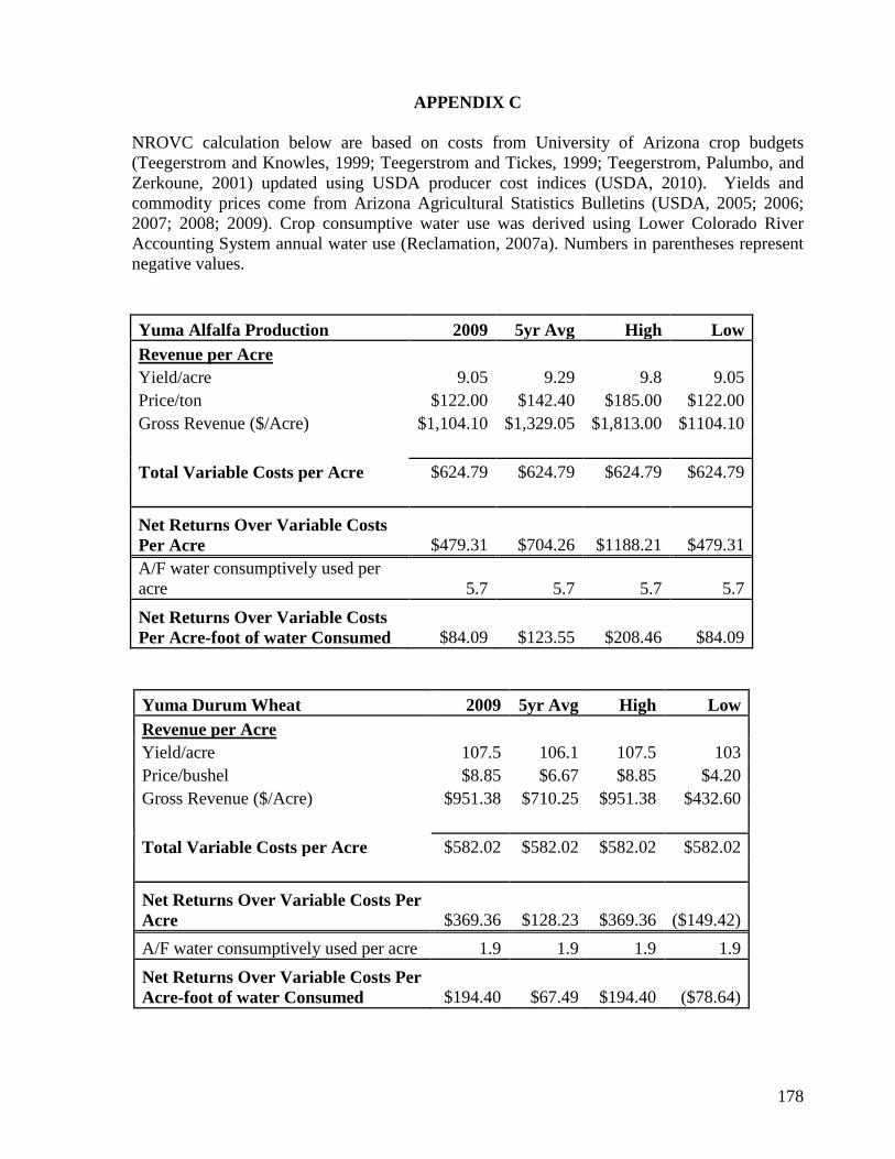
178

APPENDIX C

NROVC calculation below are based on costs from University of Arizona crop budgets (Teegerstrom and Knowles, 1999; Teegerstrom and Tickes, 1999; Teegerstrom, Palumbo, and Zerkoune, 2001) updated using USDA producer cost indices (USDA, 2010). Yields and commodity prices come from Arizona Agricultural Statistics Bulletins (USDA, 2005; 2006; 2007; 2008; 2009). Crop consumptive water use was derived using Lower Colorado River Accounting System annual water use (Reclamation, 2007a). Numbers in parentheses represent negative values.

Yuma Alfalfa Production 2009 5yr Avg High Low Revenue per Acre Yield/acre 9.05 9.29 9.8 9.05 Price/ton $122.00 $142.40 $185.00 $122.00 Gross Revenue ($/Acre) $1,104.10 $1,329.05 $1,813.00 $1104.10 Total Variable Costs per Acre $624.79 $624.79 $624.79 $624.79 Net Returns Over Variable Costs Per Acre $479.31 $704.26 $1188.21 $479.31 A/F water consumptively used per acre 5.7 5.7 5.7 5.7

Net Returns Over Variable Costs Per Acre-foot of water Consumed $84.09 $123.55 $208.46 $84.09

Yuma Durum Wheat 2009 5yr Avg High Low Revenue per Acre Yield/acre 107.5 106.1 107.5 103 Price/bushel $8.85 $6.67 $8.85 $4.20 Gross Revenue ($/Acre) $951.38 $710.25 $951.38 $432.60 Total Variable Costs per Acre $582.02 $582.02 $582.02 $582.02 Net Returns Over Variable Costs Per Acre $369.36 $128.23 $369.36 ($149.42) A/F water consumptively used per acre 1.9 1.9 1.9 1.9 Net Returns Over Variable Costs Per Acre-foot of water Consumed $194.40 $67.49 $194.40 ($78.64)

179

The most recent data for Yield/acre (lint) is from 2008 and the most recent data for Yield/acre (seed) is from 2006; thus, the table spans the years 2006-2008. LDP are not available unless county prices fall below the loan rate set by the Farm Service Agency (FSA 2010). LDP was only available in 2006.

Yuma Upland Cotton 2008 3yr Avg High Low Revenue per Acre Yield/acre (lint) 1420 1397 1420 1315 Price/pound (lint) $0.585 $0.57 $0.585 $0.53 LDP/pound $0.00 $0.029 $0.00 $0.086 Yield/acre (seed) 1.05 1.05 1.05 1.05 Price/ton (seed) $285.00 $216.67 $285.00 $167.00 Gross Revenue ($/Acre) $1,129.95 $1063.87 $1,129.95 985.39 Total Variable Costs per Acre $1,318.20 $1,318.20 $1,318.20 $1,318.20

Net Returns Over Variable Costs Per Acre ($188.25) ($254.33) ($188.25) ($332.81) A/F water consumptively used per acre 3.6 3.6 3.6 3.6 Net Returns Over Variable Costs Per Acre-foot of water Consumed ($52.29) ($70.65) ($52.29) ($92.45)

Yuma Head Lettuce 2009 5yr Avg High Low Revenues per Acre Yield/acre 345 342 345 325 Price/cwt $22.90 $17.68 $22.90 $14.60 Gross Revenue ($/Acre) $7,900.50 $6,087.00 $7,900.50 $4,582.50 Total Variable Costs per Acre $3,522.70 $3,522.70 $3,522.70 $3,522.70 Net Returns Over Variable Costs Per Acre $4,377.80 $2,564.30 $4,377.80 $1,059.80 A/F water consumptively used per acre 1.4 1.4 1.4 1.4 Net Returns Over Variable Costs Per Acre-foot of Water Consumed $3,127.00 $1,831.64 $3,127.00 $757.00

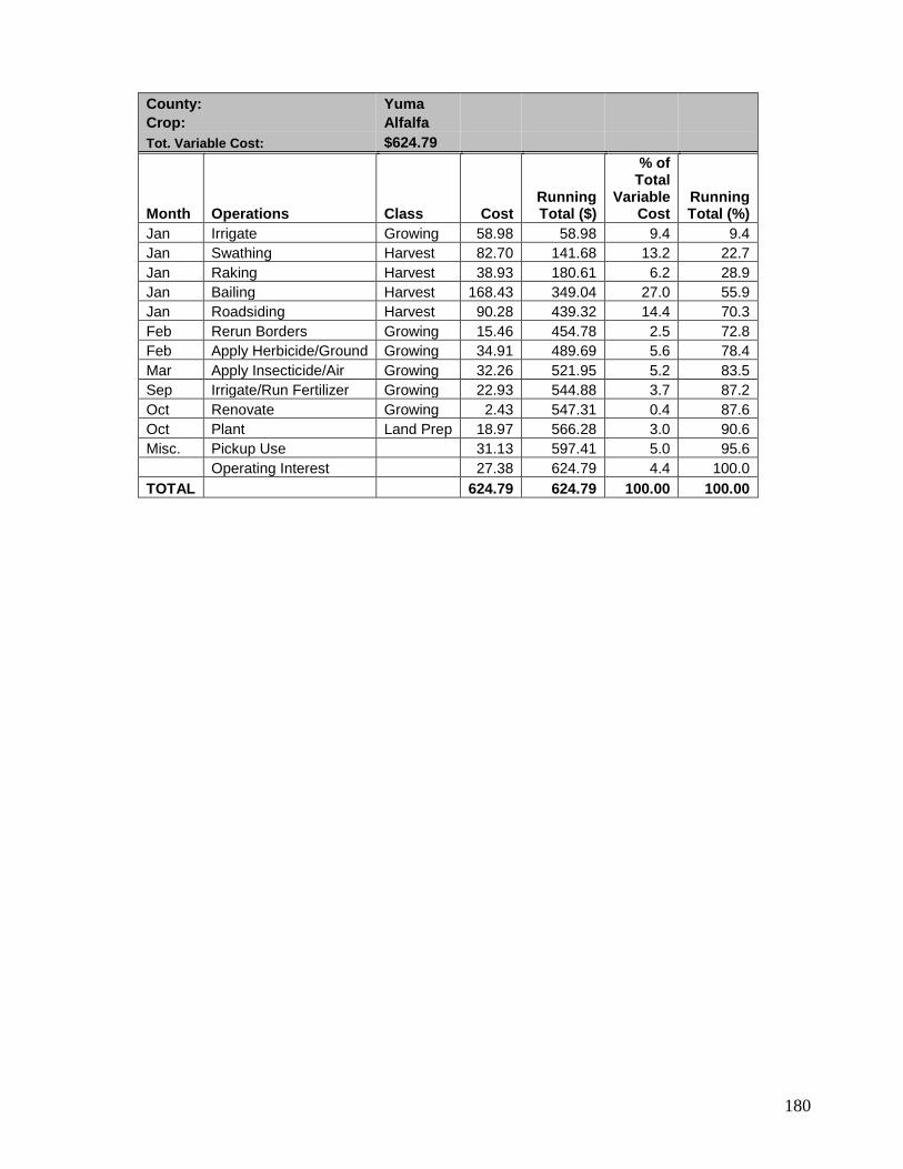
180

County: Yuma Crop: Alfalfa Tot. Variable Cost: $624.79

Month Operations Class Cost Running Total ($)

% of Total

Variable Cost

Running Total (%)

Jan Irrigate Growing 58.98 58.98 9.4 9.4 Jan Swathing Harvest 82.70 141.68 13.2 22.7 Jan Raking Harvest 38.93 180.61 6.2 28.9 Jan Bailing Harvest 168.43 349.04 27.0 55.9 Jan Roadsiding Harvest 90.28 439.32 14.4 70.3 Feb Rerun Borders Growing 15.46 454.78 2.5 72.8 Feb Apply Herbicide/Ground Growing 34.91 489.69 5.6 78.4 Mar Apply Insecticide/Air Growing 32.26 521.95 5.2 83.5 Sep Irrigate/Run Fertilizer Growing 22.93 544.88 3.7 87.2 Oct Renovate Growing 2.43 547.31 0.4 87.6 Oct Plant Land Prep 18.97 566.28 3.0 90.6 Misc. Pickup Use 31.13 597.41 5.0 95.6 Operating Interest 27.38 624.79 4.4 100.0 TOTAL 624.79 624.79 100.00 100.00

181

County: Yuma Crop: Upland Cotton Tot. Variable Cost: $1,318.20


% of Total Variable

Cost Running Total (%)

Dec Rip Land Prep 15.39 15.39 1.2 1.2 Dec Disk Land Prep 18.45 33.84 1.4 2.6 Jan Laser Level Land Prep 52.46 86.3 4.0 6.5 Jan Roll Beds Growing 3.38 89.68 0.3 6.8 Jan List Land Prep 9.96 99.64 0.8 7.6 Feb Preirrigate Growing 6.39 106.03 0.5 8.0 Mar Mulch Land Prep 7.91 113.94 0.6 8.6 Mar Plant Land Prep 11.29 125.23 0.9 9.5 Mar Remove Cap Growing 6.45 131.68 0.5 10.0 Apr Cultivate Growing 29.66 161.34 2.3 12.2 Apr Soil Fertility Growing 3.00 164.34 0.2 12.5 May Irrigate/Run Fertilizer Growing 75.37 239.71 5.7 18.2 Jun Irrigate Growing 6.39 246.1 0.5 18.7 Jun Hand Weeding Growing 100.00 346.1 7.6 26.3 Jun Apply Insecticide/Ground Growing 45.49 391.59 3.5 29.7 Jun Apply Herbicide/Ground Growing 12.21 403.8 0.9 30.6 Jul Apply Insecticide/Ground Growing 200.13 603.93 15.2 45.8 Jul Apply Insecticide/Ground Growing 14.89 618.82 1.1 46.9 Jul Hand Weeding Growing 100.00 718.82 7.6 54.5 Jul Apply Insecticide/Air Growing 14.89 733.71 1.1 55.7 Aug Apply Insecticide/Air Growing 12.66 746.37 1.0 56.6 Aug Apply Insecticide/Air Growing 16.17 762.54 1.2 57.8 Aug Irrigate/Run Fertilizer Growing 67.02 829.56 5.1 62.9 Sep Apply Insecticide/Air Growing 16.55 846.11 1.3 64.2 Sep Apply Defoliant/Air Harvest 44.44 890.55 3.4 67.6 Sep Apply Defoliant/Air Harvest 26.03 916.58 2.0 69.5 Sep Dust Control Growing 30.45 947.03 2.3 71.8 Sep Prepare Ends Harvest 1.71 948.74 0.1 72.0 Sep Cotton, First Pick Harvest 80.00 1028.74 6.1 78.0 Sep Cotton, Make Mounds Harvest 17.62 1046.36 1.3 79.4 Sep Cotton, Rood Harvest 43.33 1089.69 3.3 82.7 Sep Haul Harvest 6.80 1096.49 0.5 83.2 Sep Cotton Ginning Post Harvest 112.67 1209.16 8.5 91.7 Dec Cotton Classing Marketing 3.30 1212.46 0.3 92.0 Dec Crop Assessment Marketing 9.38 1221.84 0.7 92.7 Dec Cut Stalks Post Harvest 6.68 1228.52 0.5 93.2 Dec Disk Residue Land Prep 18.79 1247.31 1.4 94.6 Misc. Pickup Use 37.35 1284.66 2.8 97.5 Operating Interest 6% 33.54 1318.2 2.5 100.0 TOTAL 1318.20 1318.20 100.00 100.00

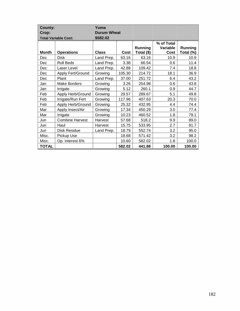
182

County: Yuma Crop: Durum Wheat Total Variable Cost: $582.02


% of Total Variable

Cost Running Total (%)

Dec Disk Land Prep. 63.16 63.16 10.9 10.9 Dec Roll Beds Land Prep. 3.38 66.54 0.6 11.4 Dec Laser Level Land Prep. 42.88 109.42 7.4 18.8 Dec Apply Fert/Ground Growing 105.30 214.72 18.1 36.9 Dec Plant Land Prep. 37.00 251.72 6.4 43.2 Jan Make Borders Growing 3.26 254.98 0.6 43.8 Jan Irrigate Growing 5.12 260.1 0.9 44.7 Feb Apply Herb/Ground Growing 29.57 289.67 5.1 49.8 Feb Irrigate/Run Fert Growing 117.96 407.63 20.3 70.0 Feb Apply Herb/Ground Growing 25.32 432.95 4.4 74.4 Mar Apply Insect/Air Growing 17.34 450.29 3.0 77.4 Mar Irrigate Growing 10.23 460.52 1.8 79.1 Jun Combine Harvest Harvest 57.68 518.2 9.9 89.0 Jun Haul Harvest 15.75 533.95 2.7 91.7 Jun Disk Residue Land Prep. 18.79 552.74 3.2 95.0 Misc. Pickup Use 18.68 571.42 3.2 98.2 Misc. Op. Interest 6% 10.60 582.02 1.8 100.0 TOTAL 582.02 441.88 100.00 100.00

183

County: Yuma Crop: Head Lettuce Tot. Variable Cost: $3,522.7


% of Total Var.

Cost

Running

Total (%)

July Rip Lnd Prep 28.10 28.1 0.8 0.8 July Disk Lnd Prep 19.11 47.21 0.5 1.3 July Laser Level Lnd Prep 27.43 74.64 0.8 2.1 July Make Borders Growing 0.64 75.28 0.0 2.1 July Preirrigate Growing 6.39 81.67 0.2 2.3 July Soil Fertility Growing 3.00 84.67 0.1 2.4 July Dust Control Growing 5.99 90.66 0.2 2.5 Aug Apply Fert/Ground Growing 115.42 206.08 3.2 5.8 Aug Apply Herbicide/Ground Growing 131.14 337.22 3.7 9.4 Sep List Lnd Prep 7.39 344.61 0.2 9.6 Aug Pre-Shape Lnd Prep 11.13 355.74 0.3 10.0 Aug Shape Beds Lnd Prep 24.12 379.86 0.7 10.6 Sep Plant Lnd Prep 135.25 515.11 3.8 14.4 Sep Bird Control Growing 6.10 521.21 0.2 14.6 Sep Set Sprinklers Growing 6.09 527.3 0.2 14.8 Sep Irrigate/Sec Sys Growing 6.97 534.27 0.2 15.0 Sep Apply Insecticide/Air Growing 32.51 566.78 0.9 15.9 Sep Field Scouting Growing 90.00 656.78 2.5 18.4 Oct Apply Insecticide/Ground Growing 33.82 690.6 0.9 19.3 Oct Apply Insecticide/Ground Growing 54.94 745.54 1.5 20.9 Sep Irrigate/Run Fertilizer Growing 23.57 769.11 0.7 21.5 Sep Remove Sprinklers Growing 6.09 775.2 0.2 21.7 Sep Make Ditches Growing 3.32 778.52 0.1 21.8 Oct Irrigate/Run Fertilizer Growing 150.29 928.81 4.2 26.0 Oct Thinning Growing 100.00 1028.81 2.8 28.8 Oct Cultivate Growing 44.02 1072.83 1.2 30.0 Oct Apply Fungicide/Ground Growing 52.38 1125.21 1.5 31.5 Oct Apply Insect/Ground Growing 11.21 1136.42 0.3 31.8 Oct Apply Insect/Air Growing 33.57 1169.99 0.9 32.7 Oct Irrigate/Run Fertilizer Growing 46.49 1216.48 1.3 34.0 Oct Hand Weeding Growing 100.00 1316.48 2.8 36.8 Oct Apply Insect/Ground Growing 26.60 1343.08 0.7 37.6 Nov Knock Borders Growing 0.64 1343.72 0.0 37.6 Nov Knock Ditches Growing 1.11 1344.83 0.0 37.6 Nov Harvest, Load and Haul Harvest 2167.20 3512.03 60.7 98.3 Dec Disk Residue Lnd Prep 9.55 3521.58 0.3 98.6 Misc. Pickup Use 31.13 3552.71 0.9 99.4 Operating Interest 6% 19.99 3572.7 0.6 100.0 Fixed Water Assessment (50.00) (50.00) TOTAL 3522.70 3522.70 100.00 100.00

184

GLOSSARY

Ascending Bid Auction - In an ascending bid procurement auction, the price starts at a relatively low level and begins to rise temporally. The winner is the bidder that first stops the ascending price and accepts that price in payment for the resource. In this way, the bidder that is willing to accept the smallest price for the resource is chosen as the winner. Bid Shading – A process by which bidders attempt to conceal their true value of the resource. In a procurement auction, bidders attempt to shade their bids in such a manner that the auctioneer believes that they value the resource more highly than they really do in an effort to obtain a premium for the resource. Budget Cap – In a water auction, a budget cap is the maximum total amount of money that the auctioneer is willing to spend to acquire the entire volume of water. Called option – Optioned water that is purchased, or called, by the contractor. Conditional Lease-back – an agreement whereby land is purchased by the entity desiring long-terms control of water and where the land is leased back to the irrigator so that farming operations may continue except when the water is needed to replace drought shortfalls. Contingent water contract – see, dry year water option contract. Contractee – In a supply reliability contract, the contractee is the party selling the option. Generally the contractees in this scenario are irrigators. Contractor – In a supply reliability contract, the contractor is the party purchasing the option to call the water in the future. Descending Bid Auction - In a descending bid procurement auction, bidders bid down the price that they will accept sequentially until no bidder wishes to bid the price down any further. The bidder that will accept the lowest price is the winner. Dry year option contract – A contract where a contractor pays the contractee a premium for the option to exercise the option at a later date. Dry-year water supply reliability contract – A contract that is designed to shift the risk of water supply variability. Under this scheme, the contractor pays the contractee a sum of money (in advance of need) for the option to call on the option at a future date. Includes both dry-year option contracts and other similar reliability contracts. Exercise payment – The payment that is made to a contractee when options are called (or exercised). Index – A method of ranking bids based upon predetermined set of criteria.

185

Iterative Auction – An auction that consists of more than one round of bidding where bidders are allowed to revise bids between rounds. Junior water rights – In a state recognizing the doctrine of prior appropriation, a junior water right holder is a person that may appropriate water but only after relatively senior right holders appropriate. Multiple Unit Auction – An auction where more than one unit is placed for auction. In the case of a multiple unit water auction, participants submit bids consisting of various volumes of water. Option premium – The amount of money paid by the contractor to the contractee to keep the option open. Procurement Auction – An auction where the auctioneer’s goal is to obtain, rather than sell, a particular item or resource. Reserve Price – In a water auction the reserve price is the maximum amount of money that the auctioneer is willing to spend per given volume of water. Revenue Equivalence – The theory that regardless of what auction design is used (ascending, descending or sealed bid), the chosen bid price is expected to be the same. Sealed Bid Auction – An auction where bidders submit confidential bids. In a procurement auction, the auctioneer obtains the confidential bids and selects the lowest bidder as the winner. Sealed Bid Multi-Unit Procurement Auction - An auction design particularly suited for water auctions because it permits the submission of bids that may vary in quantity. Senior water rights – In a state recognizing the doctrine of prior appropriation, a senior water rights holder owns rights to a relatively more secure source of water. These rights are the most valuable. Up-front payment – The payment paid to a contractee up-front in a dry year water supply reliability contract. May or may not be considered an option premium. Vickery Auction – In a procurement Vickrey auction, the winning bidder is paid the amount that the second place bidder submits. Under economic theory, this method minimized the threat of bid shading.

186

REFERENCES

Acts and Codes Alaska Water Use Act (1966) Arizona Revised Statutes, §§ 45-141, 45-172, 45-852.01. California Water Code. Cal. Code. Mississippi Water Code. Miss. Code. Sec. 53 South Dakota Water Code Sec. SD ST Sec. 46 Texas Water Code. Tex. Rev. Civ. Stat. Ann. Sec. 11 Washington Water Code. RWS Sec. 90 Cases Anon. 79 Eng. Rep. 1031 (1638). Coffin et al. v. The Left Hand Ditch Company. 6 Colo. 443. (1882). Crandall v. Woods, 8 Cal. 136 (1857). Irwin v. Phillips, 5 Cal. 140 (1855). Palmer v. Mulligan, 3 NY 307 (1805). Tyler v. Wilkinson, 24 F. Cases 427 (1827). Maps 13 Original Colonies. http://americanhistory.about.com/library/charts/blcolonial13.htm. England Precipitation Map. http://www.metoffice.gov.uk/education/secondary/students/bi_climate/es4_avg_rainfall.gif. U.S. Precipitation Map. http://www.wrcc.dri.edu/precip.html. Sources

187

Acre-foot. http://www.merriam-webster.com/dictionary/acre-foot. Anderson, T. and D. Leal. 1998. The Rise of the Enviro-Capitalists. Hover Digest, reprinted from The Wall Street Jounal. http://www.hoover.org/publications/digest/3522876.html#. Arkansas Basin River Bank. www.coloradowaterbank.org. Accessed July 1, 2009. Backman, J. 1982. Public Land Law Reform – Reflections from Western Water Law. BYU Law Review.

Bjornlund, H. 2003. “Efficient water market mechanisms to cope with water scarcity.” The International Journal of Water Resources Development 19(4), 553–567. Blackstone, W. 1765-9. Commentaries on the Laws of England. 4 vols, Oxford Clarendon Press. BOR. 2006. Agreement to Implement a Demonstration Program for System Conservation of Colorado River water, Contract No. 06-XX-30-W0451 (August 2006). BOR. 2007. Final Environmental Impact Statement: Colorado River Interim Guidelines for Lower Basin Shortages and Coordinated Operations for Lake Powell and Lake Mead, November 2007. U.S. Department of the Interior, Bureau of Reclamation. BOR. 2008a. Agreement Between the United States Bureau of Reclamation and the Yuma Mesa Irrigation and Drainage District to Implement a Demonstration Program for System Conservation of Colorado River Water, Agreement No. 08-XX-30-W0522 (Feb. 2008). BOR. 2008b. Agreement Between the United States Bureau of Reclamation and the Yuma Mesa Irrigation and Drainage District to Implement a Demonstration Program for System Conservation of Colorado River Water, Agreement No. 08-XX-30-W0534 (Oct. 2008). BOR. 2009a. Agreement Between the United States Bureau of Reclamation and the Yuma Mesa Irrigation and Drainage District to Implement a Demonstration Program for System Conservation of Colorado River Water, Agreement No. 08-XX-30-W0522 (Dec. 2009). BOR. 2009b. 2009 Water Supply Enhancement Study. United States Bureau of Reclamation. http://www.usbr.gov/mp/kbao/pilot_water_bank/index.html, Accessed October 12, 2009. BPA. 2001. www.bpa.gov/Corporate/KC/Mediacenter/pressconf/062901/customers.pdf. BPA/KC. 2001. Keeping Current. “Taking on the energy crisis: providing tools for conservation and load reduction.” May 2001. BPA. 2002. Draft Guide to Tools and Principles for a Dry Year Strategy (Guide). http://www.bpa.gov/power/pgp/dryyear/08-2002_Draft_Guide.pdf BPA. 2006. “Final Dry Year Guide” http://www.bpa.gov/power/pgp/dryyear/11-

188

2006_Final_Dry_Year_Tools_and_Principles.pdf BPA. 2008. Bonville Power Administration Website. http://www.bpa.gov/corporate/ Brookshire, D.S., B. Colby, M. Ewers, and P.T. Ganderton. 2004. “Market Prices for Water in the Semiarid West of the United States.” Water Resources Research. 40:W09S04. Brown, D. and A. Comrie. 2002. Sub-regional seasonal precipitation linkages to SOI and PDO in the Southwest United States. Atmospheric Science Letters. 3:2:94-102. Brown, T.C. 2006. “Trends in Water Market Activity and Price in the Western United States.” Water Resource Research. 42:W09402. Bryan, B., S. Gatti, J. Connor, et al. July 2005. Catchment Care – Developing an Auction Process for Biodiversity and Water Quality Gains. Report to the Onkaparinga Catchment Water Management Board. Bureau of Labor Statistics - Data. http://www.bls.gov/data/. Accessed, April 2010. Bureau of Reclamation. 2000. Brief History of the Bureau of Reclamation. www.usbr.gov/history/BRIEFHist.pdf. Accessed, April 2010. Bureau of Reclamation. 2010. Lake Mead elevation. http://www.usbr.gov/lc/region/g4000/hourly/mead-elv.html. Accessed, April 2010. Burke, S., R. Adams, and W. Wallender. 2004. Water Banks and Environmental Water Demands: Case of the Klamath Project. Water Resource Research. 40, W09S02, doi:10.1029/2003WR002832. California Association of Realtors. 2009. http://www.car.org/. Accessed March 8, 2010. CDWR. 2000. Preparing for California’s Next Drought-Changes Since 1987-1992. http://watersupplyconditions.water.ca.gov/next_drought.cfm. CDWR. 2002. DWR announces 2003 Dry Year Water Purchase Program. Press Release November 15, 2002. http://wwwowe.water.ca.gov/newsreleases/2002/11-15-02dryyear.doc Clifford, P., C. Landry and A. Larsen-Hayden. 2004. Analysis of Water Banks in the Western States. Washington Department of Ecology. Publication number 04-11-011. Climate at a Glance. 2010. NOAA website. National Climatic Data Center. http://www.ncdc.noaa.gov/oa/climate/research/cag3/cag3.html. Accessed, March 2010. Colby, B. 1990. Transactions Costs and Efficiency in Western Water Allocation. American Journal of Agricultural Economics. 72:5.

189

Colby, B. 2000. “Cap-and-Trade Policy Challenges: A Tale of Three Markets.” Land Economics. Vol. 76, No. 4. pp. 638-658. Colby, B. 2003. Water Transactions as an Urban Water Supply Strategy. Managing Urban Water Supply. Kluwer Academic Publishers. Colby, B. and K. Pittenger. 2006. Structuring Dry Year Transfers. New Mexico WRRI Conference Proceedings. Colby, B. 2007. Water resources foreword. In Lenart, M. (ed.), Global warming in the Southwest: Projections, observations, and impacts. University of Arizona, Climate Assessment of the Southwest, Tucson, Arizona. Colby, B., K. Pittenger and L. Jones. 2007. Voluntary Irrigation Forbearance to Mitigate Drought Impacts: Economic Considerations. CPI Inflation Calculator. 2010. http://data.bls.gov/cgi-bin/cpicalc.pl. Accessed March 9, 2010. Cummings, R., C. Holt, and S. Laury. 2003. Using Laboratory Experiments for Policy Making: An Example from the Georgia Irrigation Reduction Auction. Andrew Young School of Policy Studies Research Paper Series. Working Paper 06-14. Demsetz, H. 1967. Toward a Theory of Property Rights. The American Economic Review, Vol. 57, No. 2. 347-359. Deschutes. 2009. Deschutes River Conservancy. http://www.deschutesriver.org/default.aspx.

Accessed, October 2009. Dinar, A., M. Rosegrant, and R. Meinzen-Dick. 1997. Water Allocation Principles and Examples. Policy Research Working Paper No. 1779. Washington DC: World Bank and International Food Policy Research Institute. Eckhardt, G. 2009. The Edwards Aquifer Website. http://www.edwardsaquifer.net/asr.html.

Accessed June 2009. Emerick, K. 2007. Upstream Market Power in Water Transfers. Master’s Thesis, School of Agricultural and Resource Economics. The University of Arizona. GAO. 2005. Klamath River Basin: Reclamation Met its Water Bank Obligations, But Information Provided to Stakeholders Could Be Improved. GAO-05-283. Garrick, D. and K. Jacobs. 2006. Water Management on the Colorado River: From Surplus to

Shortage in Five Years. Southwest Hydrology. Garrick, D., B. Aylward, M. Siebentritt, and A. Purkey, A., eds. 2008. “Environmental Water

Transactions: Lessons Learned & Future Prospects.” 10th International River Symposium and Environmental Flows Conference.

190

Green, W.H. 2003. Econometric Analysis, 5th ed. Pearson Education. Guenther, Herbert, Chairman. 2008. Arizona Water Banking Authority Annual Plan of Operation. 2009. Håkansson, H. and I. Snehota. 2006. No Business is an Island: The Network Concept of Business Strategy. Scandinavian Journal of Management. 22:3:256-270. Hailu, A., and S. Thoyer. 2007. “Designing Multi-unit Auctions for the Allocation of Water

Scarcity.” Economic Record, 83, pp. S57-S72. Hansen, K., J. Kaplan, S. Kroll, R. Howitt. 2007. Valuing Options in California Water Markets: A Laboratory Investigation. Paper presented at the American Agricultural Economics Association Annual Meeting. Hardin, G. 1968. “The Tragedy of the Commons.” Science. 162: 1243-1248. Hartmann, H.C., 2005. Use of climate information in water resources management. In:

Encyclopedia of Hydrological Sciences, M.G. Anderson (Ed.), John Wiley and Sons Ltd., West Sussex, UK, Chapter 202.

Hartwell, R., and B. Aylward. 2007. Auctions and the Reallocation of Water Rights in Central Oregon. Dechutes River Conservancy, River Papers No. 1.

Hass, N. 2006. Drought and the Price of Water. CLIMAS Update. May, Volume 9, Number 1. http://www.climas.arizona.edu/pubs/update/may2006.pdf. Hirsch, R.M., Helsel, D.R., Cohm, T.A., and E.J. Gilroy. 1993. Statistical treatment of hydrologic data. In: Handbook of Hydrology, D.R. Maidment (Ed.), McGraw-Hill, Inc., Chapter 17. Howe, C. 1996. Increasing Efficiency in Water Markets: Examples from the Western United States. Water Marketing – The Next Generation. Eds. Anderson and Hill. Howe and Weiner. 2002. The Arkansas Water Bank Pilot Program – Progress So Far. www.isse.ucar.edu/water.../Howe%20and%20Weiner,%20Arkansas%20Water%20Ban.ppt Accessed, September 2009.

Howitt R. 1994. Empirical analysis of water market institutions: The 1991 California water market. Resource and Energy Economics, 1994, vol. 16, issue 4, pages 357-371.

Howitt, R. and J. Lund. 1999. Measuring the Economic Impacts of Environmental Reallocations of Water in California. Journal of Agricultural Economics. 81:5:1268-72. Howitt, R. and K. Hansen. 2005. “The Evolving Western Water Markets.” Choices 1st Quarter: 59-63.

191

Howitt, R., N. Moore, and R. Smith (1992). A Retrospective on California's 1991 Emergency

Drought Water Bank. Report prepared for the California Department of Water Resources. March 1992.

Idaho Department of Water Resources. 2009. http://www.idwr.idaho.gov/. Accessed, November 2009. IID. 2004a. 2003 13-Month Emergency Fallowing Program.

http://www.iid.com/Water_Index.php?pid=269 then click on 2003_Summary.pdf. IID. 2004b. Program and Proposal. http://www.iid.com/Water_Index.php?pid=273 then

2004program_proposal.pdf IID. 2007. Fallowing Programs. IID website. http://www.iid.com/Water_Index.php?pid=267 Israel, M. and J. R. Lund (1995). Recent California water transfers: implications for water

management. Natural Resources Journal, Vol. 35 (Winter): 1-32.

Jaeger, W.K. and Mikesell, R. (2002). Increasing Streamflow to Sustain Salmon and Other Native Fish in the Pacific Northwest. Contemporary Economic Policy, 20(4), 366-380.

Jenkins, M. 2008. LA Bets the Farm. High Country News. Jercich, S. 1997. California’s 1995 Water Bank Program: Purchasing Water Supply Options. Journal of Water Resources Planning and Management. 123:1 January/February. 59-65. Johnston, J. and J. DiNardo. 1996. Econometric Methods, 4th ed. McGraw-Hill/Irwin. Jones, L. 2008. Environmental Water Markets. Masters Thesis. The University of Arizona School of Agricultural and Resource Economics. Jordana, L. 1927. “Collective Irrigation Societies in Spain.” Annals of Public and Cooperative Economics. 3:3: 209-320. Kanazwa, M. 2003. Origins of Common-Law Restrictions on Water Transfers: Groundwater Law in Nineteenth Century California. The Journal of Legal Studies. 32:1: 153-180. Kennedy, P. 2003. A Guide to Econometrics, 5th ed. The MIT Press. Keplinger, Keith O., and Bruce McCarl. 1998. The 1997 Irrigation Suspension Program for the Edwards Aquifer: Evaluation and Alternatives. Texas Water Resources Institute, Technical Report No. 178. Krishna, V. 2002. Auction Theory. San Diego, CA. Academic Press. Loomis, J.B., D. Quattlebaum, T.C. Brown, and S.J. Alexander. 2003. “Expanding Institutional

192

Arrangements for Acquiring Water for Environmental Purposes: Transactions Evidence for the Western United States.” Water Resources Development. 19:21-28. Lueck, D. 1998. First Possession. The New Palgrave Dictionary of Economics and the Law. Peter Newman, Ed. Lyon, S.W., P.A. Troch, P.D. Broxton, N.P. Molotch, and P.D. Brooks. 2008. Monitoring the timing of snow melt and the initiation of streamflow using a distributed network of temperature/light sensors, Ecohydrology,Ecohydrol. 1, 215-224 DOI: 10.1002/eco.18 Maas, A. and R Anderson. 1978. And the Deserts Shall Rejoice: Conflict, Growth and Justice

in Arid Environments. MIT Press: Cambridge, Massachusetts. Mac Arthur, D. 2004. Reallocation: Leases help farms and suburbs weather drought. Headwaters. Summer. Maddaus, M., W. Maddaus. 2008. Using an End Use Model to Quantify Demand Hardening from Long-Term Conservation Programs. AWWA Water Sources Conference, Reno. http://www.awwa.org/files/Resources/Waterwiser/references/PDFs/sustainable2008_tue11- 1.pdf. Accessed July 1, 2009. Mays, L., et al. 2002. Urban Water Supply Handbook. McGraw-Hill. McClurg S. 1992. Unresolved Issues in Water Marketing. Western Water. (May/June). Milgrom, P. Summer, 1989. “Auctions and Bidding: A Primer.” The Journal of Economic Perspectives. Vol. 3, Issue 3, p 3-22. Mountain States. http://en.wikipedia.org/wiki/Mountain_States. Murray 2009. Murray Irrigation Limited. http://www.murrayirrigation.com.au/. Accessed, October 2009. MWD. 2003a. Metropolitan exercises second round of one-year water transfer options from Sacramento Valley. MWD Press Release, March 20, 2003.

http://www.mwdh2o.com/mwdh2o/pages/news/press%5Freleases/2003%2D03/watertransfer.hym.

MWD. 2003b. Improved 2003 water picture allows Metropolitan to decline final Sacramento Valley transfer option. MWD Press Release, May 1, 2003. http://www.mwdh2o.com/mwdh2o/pages/news/press%5Freleases/2003%2D05/sacrament o%5Fvalley.htm.

MWD. 2004. Metropolitan board takes steps to secure quality, reliability of Southern California water for 2005: Board agrees to store Colorado River water for Las Vegas area; authorizes pursuit of Central Valley water transfer options for 2005. MWD Press Release, Oct. 12, 2004.

193

http://www.mwdh2o.com/mwdh2o/pages/news/press%5Freleases/2004%2D10/reliability. htm.

Naeser, R. and L. Bennett. 1998. The Cost of Noncompliance: The Economic Value of Water in the Middle Arkansas River Valley. Natural Resources Journal. 38(1998): 445-463.

National Association of Realtors. 2009. http://www.realtor.org/. Accessed March 9, 2010. National Oceanic and Atmospheric Administration (NOAA). Economic Impacts of Drought and Benefits of NOAA’s Drought Forecasting Services. NOAA Magazine. (Sept. 2002). http://www.magazine.noaa.gov/stories/mag51.htm. Accessed March 2, 2010. National Oceanic and Atmospheric Administration (NOAA2). What is Pacific Decadal Oscillation? http://www.wrh.noaa.gov/fgz/science/pdo.php?wfo=fgz. Accessed, April 1, 2010. National Oceanic and Atmospheric Administration (NOAA3). Frequently Asked Questions about the Atlantic Multidecadal Oscillation (AMO). http://www.aoml.noaa.gov/phod/amo_faq.php#faq_4. Accessed, April 1, 2010. National Oceanic and Atmospheric Administration (NOAA4). Multivariate ENSO Index (MEI). http://www.esrl.noaa.gov/psd/people/klaus.wolter/MEI/. Accessed, April 1 2010. Nelson, R. 1995. Private Rights to Public Lands. Public Lands and Private Rights: The Failure of Scientific Management. Neuman, J. 1998. Beneficial Use, Waste, and Forfeiture: The Inefficient Search of Efficiency in Western Water Use. Environmental Law. Vol. 28. Newman, J. 2004. The Good, The Bad, and The Ugly: The First Ten years of the Oregon Water Trust. Nebraska Law Review. O’Donnell, M. and B. Colby. 2009a. Water Auction Design for Supply Reliability: Design,

Implementation and Evaluation. Arizona Water Institute: Enhancing Water Supply Reliability. http://www.azwaterinstitute.org/ewsrpublications.html.

O’Donnell, M. and B. Colby. 2009b. Dry-year Water Supply Reliability Contracts: A Tool for Water Managers. Arizona Water Institute: Enhancing Water Supply Reliability. http://www.azwaterinstitute.org/ewsrpublications.html. O’Donnell, M. and B. Colby. 2010. Water Banks: A Tool for Enhancing water Supply Reliability. http://www.azwaterinstitute.org/ewsrpublications.html. Oliver, I., D. Parkes. 2003. A prototype toolkit for scoring the biodiversity benefits of land use

change. Centre for Natural Resources, Department of Infrastructure, Planning and natural Resources, NSW Government.

194

Pittenger, K. 2006. Economic Arrangements to Improve Dry-Year Supply Reliability in the Lower Colorado River Basin. Master’s Thesis, School of Agricultural and Resource Economics. The University of Arizona. Pullen, J. 2006. Implications of Climate Variability on Western Water Transactions. Master’s Thesis, School of Agricultural and Resource Economics. The University of Arizona. PVID. 2004a. PVID-MWD Forbearance and Fallowing Program. Term Sheet for Forbearance and Fallowing Program Agreement. August 16, 2004. PVID. 2004b. Landowner Agreement for Fallowing in the PVID (“Landowner Agreement”) between the MWD of Southern California and PVID. Rose, C. 1990. Energy and efficiency in the realignment of common-law water rights. Journal of Legal Studies 19: 261-296. Rose, C. 1998a. “Evolution of Property Rights.” Palgrave Dictionary of Economic and the Law. Rose, C. 1998b. “Riparian Rights.” Palgrave Dictionary of Economics and the Law. Rothkopf, M., T. Teisberg, and E. Kahn. Feb., 1990. “Why Are Vickrey Auctions Rare?”. The Journal of Political Economy. Vol. 98, No. 1, pp. 94-109. Rux, A. 2008. Attitudes and Perceptions Among Water Right Holders in the Yakima Tributary. http://www.ecy.wa.gov/programs/wr/cro/images/pdfs/revauction/AnchorEnviroAttitudeske yfindings111207_r.pdf. Accessed, October 2009. SacBee 2004. Sacramento Valley's water surplus about to head south. Mike Lee, Sacramento Bee, December 18, 2004. Salas, J.D. 1993. Analysis and modeling of hydrologic time series. In: Handbook of Hydrology, D.R. Maidment (Ed.), McGraw-Hill, Inc., New York, NY, Chapter 19. Sansom, A. 2008. Texas Water Law. Water in Texas: An Introduction. University of Texas Press. Schoennagel, T., T. Veblen, W. Romme, S. Sibold, and E. Cook. 2005. ENSO and PDO Variability Affect Drought-Induced Fire Occurrence in Rocky Mountain Subalpine Forests. Ecological Applications. 15:6:2000-2014 Semitropic Water Storage District – Groundwater Banking. 2004. http://www.semitropic.com/GndwtrBankFAQs.htm. Accessed, June 2009..

195

Simpson, H. 2005. Report to the Governor and Legislature on the Arkansas River Water Bank Pilot Program. Colorado Division of Water Resources. Southern Nevada Water Authority. 2009. http://www.snwa.com/html/wr_colrvr_azbank.html. Accessed, October 2009. Staiger, D. and J.H. Stock. 1997. Instrumental Variables Regression with Weak Instruments. Econometrica. 65:557-586. Stedinger, J.R., Vogel, R.M., and F. Foufoula-Georgiou. 1993. The frequency analysis of extreme events. In: Handbook of Hydrology, D.R. Maidment (Ed.), McGraw-Hill, Inc., New York, NY, Chapter 18. Stock, J., and M. Watson. 2002. Introduction to Econometrics, United States ed. Addion Wesley. Sunding, D., Mitchell, D. and G.H. Kubota. 2004. Third-party Impacts of Land Fallowing Associated with IID-SDCWA Water Transfers 2003 and 2004.

http://www.sdcwa.org/manage/pdf/IV-QSA/EconRprtIID.pdf Teegerstrom, T. and T. Knowles. 1999. Arizon Field Crop Budgets 1999-2000: La Paz County. March. Cooperative Extension, University of Arizona. http://ag.arizona.edu/arec/ext/budgets/LaPaz-map.html. Teegerstrom, T. and B. Tickes. 1999. Arizon Field Crop Budgets 1999-2000: Yuma County. March. Cooperative Extension, University of Arizona. http://ag.arizona.edu/arec/ext/budgets/Yuma-map.html. Teegerstrom, T., J. Palumbo, and M. Zerkoune. 2001. 2000-2001 Arizona Vegetable Crop Budgets: Western Arizona. Cooperative Extension, University of Arizona. http://ag.arizona.edu/arec/ext/budgets/western.html. Teuling A.J., F. Hupet, R. Uijlenhoet, P.A. Troch. 2007. Climate variability effects on spatial soil moisture dynamics. Geophysical Research Letters. 34 (6): Art. No. L06406 Texas Water Bank 2009. http://www.twdb.state.tx.us/assistance/waterbank/waterbankMain.asp. Accessed November 2009. Tisdell, J., J. Ward, and T. Capon, 2004. The Impact of Communication and Information on a Complex Heterogeneous Closed Water Catchment Environment. USDA. Sept. 1999. Fact Sheet: Environmental Benefits Index. http://www.forestrycenter.org/library.cfm?refID=73621. Trends. 2004. 2004 Trends in Agriculture Land & Lease Values, Region Seven, American Society of Farm Managers and Rural Appraisers, California Chapter. http://www.aglandtrends.com/2004/pdfs/2004-reg07a.pdf

196

Troch P.A., et al. 2008. Dealing with Landscape Heterogeneity in Watershed Hydrology: A review of Recent Progress toward New Hydrological Theory. Geography Compass. 2: 10.1111/j.1749-8198.2008.00186.x Truckee 2009. Truckee Meadows Water Authority. http://www.tmh2o.com/. Accessed, October 2009. US Census Bureau. http://www.census.gov/popest/states/. Accessed, April 2010 USGS 2009. Irrigation Water Use. http://ga.water.usgs.gov/edu/wuir.html. Accessed, October 2009. Vickrey, W. 1961. Counterspeculation, Auctions, and Competitive Sealed Tenders. The Journal of Finance. Vol. 16, No. 1, p. 8-37. Washington Department of Water Resources. Department of Ecology – State of Washington. (2009) Aquifer Storage and Recovery. http://www.ecy.wa.gov/programs/wr/asr/asr- home.html. Accessed June 2009. Washington State Water Law – A Primer. 2006. Washington State Department of Ecology. http://www.ecy.wa.gov/pubs/98152.pdf. Publication # WR98-152. Revised July 2006. Water Bank. http://www.waterbank.com/. Accessed, October 2009. Water Education Foundation. 1996. Layperson’s Guide to Water Marketing & Transfers. Water Find 2009. Water Find National Water Brokers. http://www.waterfind.com.au/. Accessed, October 2009. Water Information Program. http://www.waterinfo.org/node/2285 . Accessed, November 2009. Water Law. http://en.wikipedia.org/wiki/Water_law Water Strategist. 1997. “ESP” Valuation of Water Contracts. Winter 10:4. Eds. R. Smith and R. Vaughan. Western States Water Laws. http://www.blm.gov/nstc/WaterLaws/alaska.html.

Wiggins, S. and G. Libecap. 1985. Oil Field Unitization: Contractual Failures in the Presence of Imperfect Information. The American Economic Review. 75:3:368-385. Williams, J. 2007. Option Markets for Water in California: Effective Management of Water Supply Risk. Willis, D., J. Caldas, M. Frasier, N. Whittlesey, J. Hamilton. 1998 The Effects of Water Rights

197

and Irrigation Technology on Streamflow Augmentation Cost in the Snake River Basin. Journal of Agricultural and Resource Economics. 23(1):225-243. Woo, C. I. Horowitz, K. Hoang. 2001. Cross Hedging and Value at Risk: Wholesale Electricity Forward Contracts. Advances in Investment and Portfolio Management. Woodka, C. Farming was Driving Force of Water Law. The Pueblo Chieftain. http://www.chieftain.com/articles/2009/02/21/news/local/doc499fc44f70f7f183600590.txt. Published February 21, 2009. Accessed March 20, 2009. Wooldrige, J.M. 2002. Econometric Analysis of Cross Section and Panel Data, 2nd ed. The MIT Press. Yardas, D. 1989. Water Transfers and Paper Rights in the Truckee and Carson River Basins. Prepared for the American Water Resources Association Symposium on “Indian Water Rights and Water Resources Management”, Missoula, Montana, June 27-30, 1989. Young, R.A. 2005. Determining the Economic Value of Water. Washington, D.C.: Resources for the Future.

Innovative Water Supply Reliability Arrangements

Documents

Transcript of Innovative Water Supply Reliability Arrangements