Quantum Algorithms for the Combinatorial Invariants of ... - idUS
126
Programa de Doctorado “Matem´ aticas” PhD Dissertation Quantum Algorithms for the Combinatorial Invariants of Numerical Semigroups Author Joaqu´ ın Ossorio Castillo Supervisor Prof. Dr. Jos´ e Mar´ ıa Tornero S´ anchez March 10, 2019
-
Upload
khangminh22 -
Category
Documents
-
view
1 -
download
0
Transcript of Quantum Algorithms for the Combinatorial Invariants of ... - idUS

Programa de Doctorado “Matematicas”
PhD Dissertation
Quantum Algorithms for theCombinatorial Invariants of
Numerical Semigroups
AuthorJoaquınOssorio Castillo
SupervisorProf. Dr. Jose Marıa
Tornero Sanchez
March 10, 2019


A mi abuela Marıa

2
Agradecimientos
Hay varias personas a las que me gustarıa agradecer su contribucion, directa oindirecta, a esta tesis doctoral.
En primer lugar, a Jose Marıa Tornero, por aceptarme como discıpulo alla por2013 y por abrirme las puertas no solo de la investigacion sino tambien de su casa(aunque solo fuese una vez, pero bueno algo es algo). Por todas las conversacionesy discusiones interesantes que hemos tenido a lo largo de estos anos (algunas deellas incluso sobre matematicas), y por adaptarse siempre a mis caoticos ritmos detrabajo y a quedar para tomar algo los domingos a las 9 de la manana habiendoavisado a las 8:55 tras tres meses sin dar senales de vida (es posible que este siendoun poco exagerado, aunque por ahı debe andar la cosa). Soy consciente de que estatesis doctoral nunca habrıa sido posible con otro director. O sı, quien sabe, ya casinada me sorprende, aunque lo veo bastante improbable. Ah, por cierto, he encon-trado una excusa perfecta para que sigamos trabajando juntos despues de esto, note vas a librar de mı tan facilmente. Pero primero vamos a lo que vamos... Readyto save the world again?
A Julio Gonzalez y a Fran Pena, de la Universidad de Santiago de Compostela,por acogerme en su grupo de investigacion durante mis primeros anos en Galicia, ypor todo lo que he aprendido junto a ellos de optimizacion matematica y de com-putacion cuantica adiabatica. Al principio de esta aventura ambas ramas me erancompletamente desconocidas, y al final terminaron siendo una parte fundamentalde esta tesis doctoral. A mis companeros del ITMATI, y en especial a Diego y aGabriel, por su infinita paciencia a la hora de ensenarme a desarrollar de verdad(vamos, a programar en linux y a usar git). Tambien me gustarıa agradecer denuevo a Fran y al resto de miembros del tribunal, Jorge Ramırez Alfonsın, JesusSoto, Fernando Sancho e Ignacio Ojeda, por acceder a evaluar esta tesis y sobre todopor darme la oportunidad de discutir personalmente con ellos los resultados de esta.
Echando la vista atras, las matematicas no siempre me gustaron, e incluso lleguea aborrecerlas en algun momento de mi vida. Me gustarıa agradecer a dos grandes(y eternos) amigos, Rafa y Juan Pablo, las horas que dedicaron durante el institutoa ayudarme a sacar esta materia adelante. Gracias a ellos descubrı durante aquel-los anos tan importantes que las matematicas no solo no son difıciles, sino que sonhermosas. Una lastima que acabaran como ingenieros...
A lo largo de mi epoca universitaria y laboral me perdı tres veces, y tres veces mevolvı a encontrar. Gracias Rosa, debido a tu testimonio y a tus consejos fui capaz deadentrarme a estudiar matematicas cuando ya llevaba cuatro anos en la universidad,

4
una decision que en su dıa fue difıcil pero de la que jamas me he arrepentido y de laque jamas me arrepentire. Gracias Maca, por compartir tu experiencia conmigo yensenarme lo bonita que es la investigacion, y tambien por hacer de celestina entreel Sr. Tornero y yo (aunque supongo que el tendra una opinion diferente sobre siagradecerte esto o no...). Y gracias Manu, por mostrarme el camino para llegar aSantiago, y por acogerme como a un hermano durante aquellos primeros meses deadaptacion a la lluvia y a los churros frıos.
Al resto de amigos matematicos que tengo repartidos por el mundo, pero enespecial a los que siguen siendo una parte importante de mi vida y que espero siganahı siempre. Ale, Fran, Jara, Jesus, Jose Luis, Manolo, Pedro (y Maca y Manu, queya los mencione antes pero que tambien merecen estar aquı), gracias por ensenarmedurante aquellos maravillosos anos el verdadero significado de la universidad.
A mis padres, Joaquın y Ana, y a mi hermano, Jose Marıa, porque han estadoahı en mis buenas y malas decisiones y me han ensenado a trabajar duro y a sac-rificarme por mis objetivos. Equivocarse siempre ha sido mucho mas facil sabiendoque ellos estarıan detras para levantarme. A mi querida mujer, Leti, a quien conocıal poco de empezar esta tesis doctoral y que la ha vivido de cerca durante casisu totalidad (pobrecita... seguro que estareis pensando). Sin tu apoyo todo estohabrıa sido mucho mas difıcil; gracias por estar a mi lado, y por querer compartirlos buenos y malos momentos conmigo. Soy el que soy gracias a vosotros; siemprehabeis creıdo en mı y me habeis apoyado, incluso cuando yo no lo hacıa. Esta tesisdoctoral es tan vuestra como mıa. Un agradecimiento especial para mi perro, Bebo,por calentarme los pies mientras estaba trabajando en esto y por fingir tener quebajar a mear cada vez que veıa que llevaba demasiadas horas sentado en la silla.
Gracias a todos. :)
Santiago de Compostela, 10 de marzo de 2019


ii

Contents
1 Introduction 3
2 Numerical Semigroups and the Frobenius problem 52.1 Numerical Semigroups . . . . . . . . . . . . . . . . . . . . . . . . . . 52.2 Computational Complexity Theory . . . . . . . . . . . . . . . . . . . 112.3 Computational Complexity of the Frobenius Problem and the NSMP 16
3 Quantum Computation 253.1 Introduction . . . . . . . . . . . . . . . . . . . . . . . . . . . . . . . . 253.2 Quantum Turing Machines . . . . . . . . . . . . . . . . . . . . . . . . 263.3 Quantum Bits and Quantum Entanglement . . . . . . . . . . . . . . . 273.4 Quantum Circuits . . . . . . . . . . . . . . . . . . . . . . . . . . . . . 353.5 Adiabatic Quantum Computing . . . . . . . . . . . . . . . . . . . . . 38
4 Quantum Algorithms 434.1 Introduction . . . . . . . . . . . . . . . . . . . . . . . . . . . . . . . . 434.2 Deutsch’s Algorithm . . . . . . . . . . . . . . . . . . . . . . . . . . . 444.3 Deutsch–Jozsa Algorithm . . . . . . . . . . . . . . . . . . . . . . . . . 474.4 Simon’s Algorithm . . . . . . . . . . . . . . . . . . . . . . . . . . . . 514.5 Shor’s Factoring Algorithm . . . . . . . . . . . . . . . . . . . . . . . . 564.6 Grover’s Search Algorithm . . . . . . . . . . . . . . . . . . . . . . . . 674.7 Quantum Counting . . . . . . . . . . . . . . . . . . . . . . . . . . . . 80
5 Quantum Algorithms for the Combinatorial Invariants of Numeri-cal Semigroups 875.1 Introduction . . . . . . . . . . . . . . . . . . . . . . . . . . . . . . . . 875.2 The numsem library . . . . . . . . . . . . . . . . . . . . . . . . . . . . 885.3 Sylvester Denumerant and Numerical Semigroup Membership . . . . 905.4 Apery Set and Frobenius Problem . . . . . . . . . . . . . . . . . . . . 96
6 Conclusions and Future Work 109
7 Bibliography 111
1

2 CONTENTS
1
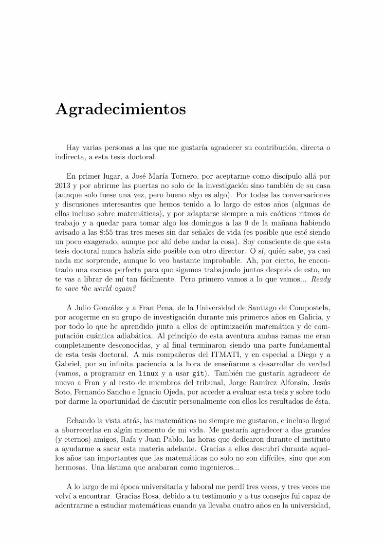
Introduction
“You have nothing to do but mention the quantum theory, and peoplewill take your voice for the voice of science, and believe anything.”
– George Bernard Shaw, Geneva, a Fancied Page of History in Three Acts
It was back in spring 2014 when the author of this doctoral dissertation wasfinishing its master thesis, whose main objective was the understanding of PeterW. Shor’s most praised result, a quantum algorithm capable of factoring integers inpolynomial time. During the development of this master thesis, me and my yet-to-be doctoral advisor studied the main aspects of quantum computing from a purelyalgebraic perspective. This research eventually evolved into a sufficiently thoroughcanvas capable of explaining the main aspects and features of the mentioned algo-rithm from within an undergraduate context.
Just after its conclusion, we seated down and elaborated a research plan for afuture Ph.D. thesis, which would expectantly involve quantum computing but alsoa branch of algebra whose apparently innocent definitions hide some really hardproblems from a computational perspective: the theory of numerical semigroups.As will be seen later, the definition of numerical semigroup does not involve so-phisticated knowledge from any somewhat obscure and distant branch of the treeof mathematics. Nonetheless, a number of combinatorial problems associated withthese numerical semigroups are extremely hard to solve, even when the size of theinput is relatively small. Some examples of these problems are the calculations ofthe Frobenius number, the Apery set, and the Sylvester denumerant, all of thembearing the name of legendary mathematicians.
This thesis is the result of our multiple attempts to tackle those combinato-rial problems with the help of a hypothetical quantum computer. First, Chapter2 is devoted to numerical semigroups and computational complexity theory, and isdivided into three sections. In Section 2.1, we give the formal definition of a numer-ical semigroup, along with a description of the main problems involved with them.In Section 2.2, we sketch the fundamental concepts of complexity theory, in orderto understand the true significance within the inherent hardness concealed in theresolution of those problems. Finally, in Section 2.3 we prove the computationalcomplexity of the problems we aim to solve.
3

4 1. INTRODUCTION
Chapter 3 is the result of our outline of the theory of quantum computing.We give the basic definitions and concepts needed for understanding the particularplace that quantum computers occupy in the world of Turing machines, and alsothe main elements that compose this particular model of computation: quantumbits and quantum entanglement. We also explain the two most common models ofquantum computation, namely quantum circuits and adiabatic quantum comput-ers. For all of them we give mathematical definitions, but always having in mindthe physical experiments from which they stemmed.
Chapter 4 is also about quantum computing, but from an algorithmical perspec-tive. We present the most important quantum algorithms to date in a standardizedway, explaining their context, their impact and consequences, while giving a math-ematical proof of their correctness and worked-out examples. We begin with theearly algorithms of Deutsch, Deutsch-Jozsa, and Simon, and then proceed to ex-plain their importance in the dawn of quantum computation. Then, we describe themajor landmarks: Shor’s factoring, Grover’s search, and quantum counting.
Chapter 5 is the culmination of all previously explained concepts, as it includesthe description of various quantum algorithms capable of solving the main problemsinside the branch of numerical semigrops. We present quantum circuit algorithmsfor the Sylvester denumerant and the numerical semigroup membership, and adia-batic quantum algorithms for the Apery Set and the Frobenius problem. We alsodescribe a C++ library called numsem, specially developed within the context of thisdoctoral thesis and which helps us to study the computational hardness of all pre-viously explained problems from a classical perspective.
This thesis is intended to be autoconclusive at least in the main branches of math-ematics in which it is supported ; that is to say numerical semigroups, computationalcomplexity theory, and quantum computation. Nevertheless, for the majority ofconcepts explained here we give references for the interested reader that wants todelve more into them.

2
Numerical Semigroups and theFrobenius problem
“One Ring to rule them all, One Ring to find them,One Ring to bring them all and in the darkness bind themIn the Land of Mordor where the Shadows lie.”
– J. R. R. Tolkien, The Lord of the Rings
2.1 Numerical Semigroups
The study of numerical semigroups has its origins at the end of the 19th Century,when English mathematician James Joseph Sylvester (1814 – 1897) and Germanmathematician Ferdinand Georg Frobenius (1849 – 1917) were both interested inwhat is now known as the Frobenius problem, which we proceed to enunciate.
Definition 2.1.1. Let a1, a2, . . . , an ∈ Z≥0 with gcd(a1, a2, . . . , an) = 1, the Frobe-nius problem, or FP, is the problem of finding the largest positive integer that cannotbe expressed as an integer conical combination of these numbers, i.e., as a sum
n∑j=1
λiai with λi ∈ Z≥0.
This problem, so easy to state, can be extremely complicated to solve in themajority of cases, as will be seen in Section 2.3. It can be found in a wide variety ofcontexts, being the most famous the problem of finding the largest amount of moneywhich cannot be obtained with a certain set of coins: if, for example, we have anunlimited amount of coins of 2 and 5 units, we can represent any quantity except 1and 3.
In order to understand the relationship between this problem and numericalsemigroups, we shall first define the latter.
Definition 2.1.2. A semigroup is a pair (S,+), where S is a set and + is a binaryoperation + : S × S → S that is associative.
Definition 2.1.3. A numerical semigroup S is a subset of the non-negative integersZ≥0 which is closed under addition, contains the identity element 0, and has a finitecomplement in Z≥0.
5

6 2. NUMERICAL SEMIGROUPS AND THE FROBENIUS PROBLEM
From now on, we shall denote numerical semigroups as S, taking for grantedthat they are commutative and that their associated operation is the addition. As itcan be easily noted, a numerical semigroup is trivially a semigroup. In other words,a numerical semigroup is a semigroup that, additionally, is a monoid (i.e., it alsohas an identity element) and has finite complement in Z≥0. In order to work withnumerical semigroups, it will be necessary to characterize them somehow. For that,let us set forth the following lemma.
Lemma 2.1.4. Let A = a1, ..., an be a nonempty subset of Z≥0. Then,
S = 〈A〉 = 〈a1, ..., an〉 = λ1a1 + ...+ λnan | λi ∈ Z≥0
is a numerical semigroup if and only if gcd(a1, ..., an) = 1.
Proof. Assume S to be a numerical semigroup with gcd(a1, . . . , an) = d and letx = max(Z≥0\S) —as Z≥0\S is finite, it has a maximum—. If s ∈ S, then d|s.As x+1 ∈ S and x+2 ∈ S, then d | (x+1) and d | (x+2), which implies that d = 1.
Let S = 〈A〉 = 〈a1, ..., an〉 with gcd(a1, . . . , an) = 1, then by Bezout’s identity[23] there exist integers x1, x2, . . . , xn ∈ Z such that a1x1 + a2x2 + · · · + anxn = 1.If a1x1 + · · ·+ anxn = p+ q, where p contains the positive terms and q the negativeones, then p = 1− q. We can define r = −q and, as p ∈ S, r ∈ S and r+ 1 ∈ S. Lets ≥ (r−1)r+(r−1), and let t and u such that s = tr+u with 0 ≤ u < r. It followsthat u ≤ r − 1 ≤ t and finally we have that s = u(r + 1) + (t − u)r ∈ S. Thus, Shas finite complement in Z≥0 and consequently is a numerical semigroup.
The previous lemma tells us that, drawing from a set A ⊆ Z≥0, it is possibleto generate a semigroup S = 〈A〉 as long as the elements of A satisfy a certaincondition. In this context, any set A such that S = 〈A〉 for a certain numericalsemigroup S is called a system of generators of S. Even more, it can be proved thatany numerical semigroup can be expressed that way, as will be shown next.
Theorem 2.1.5. Every numerical semigroup S admits a unique minimal system ofgenerators, which can be calculated as S∗ \ (S∗ + S∗) with S∗ = S \ 0.
Proof. Let S∗ = S \ 0 and let s ∈ S∗. If s /∈ S∗ \ (S∗ + S∗), then s ∈ S∗ + S∗ andthere exist t, u ∈ S∗ such that s = t+u. As t, u < s, we can repeat this procedure afinite number of steps until we find s1, . . . , sn ∈ S∗ \ (S∗+S∗) with s = s1 + · · ·+sn.Thus, we can conclude that S∗ \ (S∗ + S∗) is a system of generators of S.
Besides, let A be a system of generators of S and let s ∈ S∗\(S∗+S∗), then thereexist t ∈ Z>0, λ1, . . . , λn ∈ Z≥0 and a1, . . . , an ∈ A such that s = λ1a1 + · · ·+ λnan.As s /∈ S∗+S∗, we have that s = ai for a certain i ∈ 1, . . . , n and thus S∗\(S∗+S∗)is contained in any system of generators of S.
Corollary 2.1.6. Let S be a numerical semigroup generated by A = a1, . . . , anwith 0 6= a1 < a2 < ... < an. Then, A is a minimal system of generators of S if andonly if ai+1 /∈ 〈a1, a2, . . . , ai〉, for all i ∈ 1, . . . , n− 1.
It will be proven later in this section that the minimal system of generators ofa numerical semigroup is in fact finite. Hereinafter, if we say that S = 〈A〉 with

2.1. NUMERICAL SEMIGROUPS 7
A = a1, a2, . . . , an is a numerical semigroup, then we shall assume without lossof generality that a1 < a2 < · · · < an, gcd(a1, a2, . . . , an) = 1, and that A is theminimal system of generators of S. Some examples of numerical semigroups, whichwill be used for the rest of the section, are:
Sa = 〈3, 7〉 = 0, 3, 6, 7, 9, 10, 12,→Sb = 〈4, 9〉 = 0, 4, 8, 9, 12, 13, 16, 17, 18, 20, 21, 22, 24,→Sc = 〈5, 8, 11〉 = 0, 5, 8, 10, 11, 13, 15, 16, 18,→Sd = 〈5, 7, 9〉 = 0, 5, 7, 9, 10, 12, 14,→
Where → means that all integers thenceforth are also included in the numericalsemigroup. Having thus defined and characterized what numerical semigroups are,we proceed to describe some of their combinatorial invariants.
Definition 2.1.7. Let S = 〈a1, a2, . . . , an〉 be a numerical semigroup, then
m(S) = a1 and e(S) = n
are called respectively the multiplicity of S and the embedding dimension of S.
Lemma 2.1.8. Let S be a numerical semigroup, then
m(S) = minS∗
Definition 2.1.9. The set of gaps of a numerical semigroup S is defined as
G(S) = Z≥0\S.
Its cardinal,g(S) = |G(S)|,
is called the genus of S; and its maximum,
f(S) = maxG(S),
is called the Frobenius number of S.
In other words, as by definition any numerical semigroup S has a finite comple-ment in Z≥0, we can define the maximum of such complement as f(S), known asthe Frobenius number. In fact, the Frobenius problem described at the beginning ofthis chapter in Definition 2.1.1 can be enunciated as the problem of finding f(S) fora certain numerical semigroup S. We shall expand the concepts related to the diffi-culties that surround the calculation of the Frobenius number in Section 2.3. Table2.1 shows the combinatorial invariants associated for the previously given examplesof semigroups.
Greek-French mathematician Roger Apery (1916 – 1994), better known for prov-ing in 1979 the irrationality of ζ(3) [11], also laid the background in the context ofthe resolution of singularities of curves [10] for an important set associated to anumerical semigroup S and one of its elements.

8 2. NUMERICAL SEMIGROUPS AND THE FROBENIUS PROBLEM
S A m(S) e(S) G(S) g(S) f(S)Sa 〈3, 7〉 3 2 1, 2, 4, 5, 8, 11 6 11Sb 〈4, 9〉 4 2 1, 2, 3, 5, 6, 7, 10, 11, 14, 15, 19, 23 12 23Sc 〈5, 8, 11〉 5 3 1, 2, 3, 4, 6, 7, 9, 12, 14, 17 10 17Sd 〈5, 7, 9〉 5 3 1, 2, 3, 4, 6, 8, 11, 13 8 13
Table 2.1: Combinatorial invariants for some examples of semigroups
Definition 2.1.10. The Apery set of a numerical semigroup S with respect to acertain s ∈ S∗ is defined as
Ap(S, s) = x ∈ S | x− s /∈ S.
A possible characterization of the elements of the Apery set one by one, whichwill come to special use in Chapter 5, is given by the following lemma.
Lemma 2.1.11. Let S be a numerical semigroup and let s ∈ S∗. Then, Ap(S, s) =ω0, ω1, ..., ωs−1 where ωi is the least element of S congruent with i modulo s, forall i ∈ 0, ..., s− 1. Consequently, |Ap(S, s)| = s.
Proof. Let x ∈ Ap(S, s). Then, by definition, x ∈ S and x − s /∈ S. As x ≡ imod s for a certain i ∈ 0, . . . , s − 1, it follows that x = ωi. As a result,Ap(S, s) ⊆ ω0, . . . , ωs−1.
Also, let ωi = minx ∈ S | x ≡ i mod s, it is clear that ωi ∈ S and ωi− s /∈ S.Thus, ω0, . . . , ωs−1 ⊆ Ap(S, s).
By means of an example on how to calculate the Apery set of a semigroup withrespect to a certain element, let
Sc = 〈5, 8, 11〉 = 0, 5, 8, 10, 11, 13, 15, 16, 18,→.
Then Ap(Sc, 5) = ω0, . . . , ω4, where
ω0 = minx ∈ S | x ≡ 0 mod 5 = 0
ω1 = minx ∈ S | x ≡ 1 mod 5 = 11
ω2 = minx ∈ S | x ≡ 2 mod 5 = 22
ω3 = minx ∈ S | x ≡ 3 mod 5 = 8
ω4 = minx ∈ S | x ≡ 4 mod 5 = 19
We proceed to prove some results via the properties of the Apery set.
Proposition 2.1.12. The minimal system of generators of a numerical semigroupS is finite.
Proof. Let s ∈ S∗. Then, it is easy to see that for every t ∈ S there exists aunique pair (u, v) ∈ Z≥0 × Ap(S, s) such that t = us + v. Thus, S is generated byA = Ap(S, s) ∪ s and, as A is finite, the unique minimal system of generatorsmust be finite.
2.1. NUMERICAL SEMIGROUPS 9
Lemma 2.1.13. Let S be a numerical semigroup, then
e(S) ≤ m(S).
Proof. Let a = m(S) and let A = Ap(S, a) ∪ a. Thus, as S can be generated byA \ 0 and |A \ 0| = a, we can conclude that e(S) ≤ m(S).
The Apery set is noteworthy in the context of the Frobenius problem as thereexists a relationship between its members (regardless of the element s ∈ S∗ wechoose) and the Frobenius number, which we proceed to enunciate and prove.
Theorem 2.1.14. (A. Brauer – J. E. Shockley, 1962) [31] Let S be a numericalsemigroup and let s ∈ S∗. Then
f(S) = maxAp(S, s)− s
g(S) =1
s
∑ω∈Ap(S,s)
ω
− s− 1
2
Proof. As Ap(S, s) = x ∈ S | x−s /∈ S, we have that maxAp(S, s)−s /∈ S. Lety > maxAp(S, s) − s, then y + s > maxAp(S, s). Let z ∈ Ap(S, s) such thatz ≡ y + s mod s, then as z < y + s we have that y = z + ks for some k ≥ 0, hencey − s = z + (k − 1)s ∈ S. This proves the first identity.
As for the genus of S, for every w ∈ Ap(S, s), w ≡ i mod s with i ∈ 0, . . . , s−1implies that there exists ki ∈ Z≥0 such that w = kis+ i. This way, we can write theelements of the Apery Set as ωi = kis+ i for i ∈ 0, . . . , s− 1.
Thus, as x ≡ ωi mod s implies that x ∈ S if and only if ωi ≤ x, then we canconclude that
g(S) =s−1∑i=1
ki =1
s
s−1∑i=1
(kis+ i)− s− 1
2=
1
s
s−1∑i=1
ωi −s− 1
2.
Now we exemplify the relationship between numerical semigroups and combi-natorial optimization, as one of the most important problems in the latter branchof mathematics, known as the knapsack problem or rucksack problem, and moreconcretely one of its variants [93] (p. 374), can be seen as the problem of decidingif a given integer t belongs to a certain numerical semigroup S.
Definition 2.1.15. The numerical semigroup membership problem, or NSMP, isthe problem of determining if, given a certain integer t ∈ Z≥0 and a numericalsemigroup S = 〈a1, ..., an〉, the integer t is contained in S. That is to say, if thereexist non-negative integers λ1, . . . , λn ∈ Z≥0 such that
n∑i=1
λiai = t.

10 2. NUMERICAL SEMIGROUPS AND THE FROBENIUS PROBLEM
Finally, we show another important problem in numerical semigroups related tothe previous one. In the mid-19th century, J. J. Sylvester studied the number ofpartitions of an integer with respect to a certain subset of non-negative integers[109, 110]. In the context of this chapter, this problem can be seen as an extensionof the NSMP, but rather than answering whether or not an integer is contained ina numerical semigroup, we go farther and want to calculate the number of distinctrepresentations of that integer with respect to the minimal system of generators ofthe semigroup.
Definition 2.1.16. The Sylvester denumerant of a non-negative integer t ∈ Z≥0
with respect to a numerical semigroup S = 〈a1, ..., an〉, denoted by d(t, S) or byd(t; a1, . . . , an), is defined as the number of solutions of the Diophantine equation
n∑i=1
λiai = t,
where λ1, . . . , λn ∈ Z≥0.
By means of an example, we recall the previously defined semigroup:
Sd = 〈5, 7, 9〉 = 0, 5, 7, 9, 10, 12, 14,→
The Frobenius number of Sd is equal to f(Sd) = 13, which means that anyinteger greater than 13 is contained in the semigroup. However, the number ofpossible representations may differ between them. Number 15, for example, has aunique representation with respect to 5, 7 and 9:
15 = 3× (5) + 0× (7) + 0× (9),
while on the other hand, number 14 has two possible representations:
14 = 1× (5) + 0× (7) + 1× (9)
and
14 = 0× (5) + 2× (7) + 0× (9).
This tells us that d(15; 5, 7, 9) = 1 and d(14; 5, 7, 9) = 2.
The study of the Sylvester denumerant is of great importance in many branchesof mathematics and, as can be easily deduced, is at least as hard to solve as thenumerical semigroup membership problem. This result will be formally explainedin Section 2.3.
A thorough study of numerical semigroups can be found in the book by J. C.Rosales and P. A. Garcıa-Sanchez [101]. The majority of problems and definitionssurrounding the Frobenius number and the Sylvester denumerant can be found inthe book by J. L. Ramırez-Alfonsın [98].

2.2. COMPUTATIONAL COMPLEXITY THEORY 11
2.2 Computational Complexity Theory
The aim of this section is to provide a background on computational complex-ity theory, a branch of mathematics and computer science which focuses on thedefinition of classes of computational problems in accordance with their inherentdifficulty, and on the relationships between those classes.
This framework will become useful for two of the main objectives of this Ph.D.thesis: first, for placing the Frobenius problem within the context of those prob-lem classes —i.e., what does exactly mean that the Frobenius problem is hard tosolve—; and second, for contextualizing the quantum model of computation insidethe universal Turing machines used for standardizing the aforementioned classesof problems. In order to achieve that, we begin by defining two basic ingredientsneeded for this problem classification.
Definition 2.2.1. [62, 77] A decision problem or recognition problem Π is a functionwith a one-bit output: YES or NO —i.e., a problem that can be posed as a yes-noquestion of the input—. To specify a decision problem, one must define the set A ofpossible inputs and the subset B ⊆ A of YES instances.
In the context of automata and abstract computers, it is necessary to define anew concept that generalizes the notion of a machine capable of solving a certain de-cision problem. We give from now on some essential notions of the so-called Turingmachines, named after English computer scientist and mathematician Alan Turing(1912 – 1954) and its groundbreaking and dazzling work [111]. These machinesmay appear to be simple or limited, but they are capable of simulating any com-puter algorithm and of doing everything that a real computer can do [108]. Moreinformation on the subject can be found in [77].
Definition 2.2.2. A deterministic Turing machine M, or DTM, is defined by atriple M = (S,Σ, δ), where S is a finite set of states (with an initial state s0 ∈ Sand a set of final states F ⊆ S), Σ is an alphabet containing at least the blank symbol#, and δ : S \ F × Σ → S × Σ × L,R is a partial function called the transitionfunction.
The definition of Turing machine is quite abstract, but it can be seen as a devicethat manipulates symbols on a strip of tape according to a table of rules. This tapeis divided into cells, each of them containing a symbol from the alphabet Σ, andthe machine has a head that reads or writes on the tape and moves the tape left orright. The machine follows a single and deterministic computation path starting inthe state s0 and ending in one of the final states. A representation of this path isshown in Figure 2.1.
Now that we have defined what a deterministic Turing machine is, we can starta classification of decision problems with respect to them.
Definition 2.2.3. The class P, or PTIME, contains all decision problems solvableby a deterministic Turing machine using a polynomial amount of computation timewith respect to the size of the input.

12 2. NUMERICAL SEMIGROUPS AND THE FROBENIUS PROBLEM
S0
S1
S2
SF
Figure 2.1: Example of computation of a deterministic Turing machine
Figure 2.2: Example of computation of a non-deterministic Turing machine
The class P is known to contain many elemental problems in mathematics, likeaddition and multiplication, and other not so elemental such as the problem of de-ciding whether an integer is prime [7], or the resolution of a certain type of linearoptimization problem [12, 73].
Another concept that generalizes the notion of a Turing machine one step furtheris the following:
Definition 2.2.4. A non-deterministic Turing machine M, or NTM, is defined bya triple M = (S,Σ, δ), where S is a finite set of states (with an initial state s0 ∈ Sand a set of final states F ⊆ S), Σ is an alphabet containing at least the blank symbol# and δ ⊆ (Q \A×Σ)× (Q×Σ×L,R) is a relation on states and symbols calledthe transition relation.
As can be seen, the only difference between a deterministic Turing machine anda non-deterministic Turing machine is the substitution of the transition functionfor a transition relation. This distinction can be interpreted as a change in thecomputation path followed by the machine. While in the deterministic Turing ma-chine the transition between a state and the next is deterministic and unique, in thenon-deterministic Turing machine there can be more than one state after a certainstep in the computation. The computation path may branch after a state, makingan indeterminate number of copies of the machine which will continue working inparallel. Thus, instead of a computation path, the behavior of a non-deterministic

2.2. COMPUTATIONAL COMPLEXITY THEORY 13
Turing machine is better seen as a computation tree, represented in Figure 2.2.
Although the concept of a non-deterministic Turing machine is more philosophi-cal than realistic and has not been implemented in practice, there have been recentdesigns of a model for non-deterministic Turing machine that exploit the ability ofDNA to replicate itself [40].
In the same way as with deterministic Turing machines, we can also classify alldecision problems with respect to the non-deterministic Turing machines.
Definition 2.2.5. The class NP contains all decision problems that can be solved bya non-deterministic Turing machine that runs in polynomial time with respect to thesize of the input. If the answer is YES, then at least one computation path accepts.On the other hand, if the answer is NO, all computation paths must reject.
Another interpretation of the set of decision problems that are contained in NPstates that a problem is solvable by a non-deterministic Turing machine in polyno-mial time if and only if the problem of veryfing if a certain polynomial-size proof ofthis fact is correct is in P. In other words, the statements verifiable in polynomialtime by a deterministic Turing machine and solvable in polynomial time by a non-deterministic Turing machine are totally equivalent, and a proof of this fact canbe found in [108]. For example, the problem of finding a prime factor of a certaininteger N , also called prime factorization, is not known to be in P. Nevertheless, asthe problem of determining if a certain prime p is a factor of N can be checked inpolynomial time, we know that prime factoring is in NP.
As a deterministic Turing machine is also trivially a non-deterministic Turingmachine, it is easy to conclude that P ⊆ NP. However, the question of whetherthere exists a problem in NP that is not in P is one of the most important openproblems in theoretical computer science —and in mathematics in general—, and
is known as the P versus NP problem, or P?= NP. In other words, does the non-
determinism of a Turing machine make a difference? Intuitively, one might say itshould, but that remains to be proven. Interesting surveys about this subject canbe found in [107], [38] and [4].
Apart from all problems in P, a myriad of compelling problems in mathematicsare also known to be in NP, such as the previously mentioned prime factorization,the Boolean satisfiability problem —also known as SAT— and many others. In fact,the SAT problem was the first to be proven to be complete for the class NP [37], aconcept which we proceed to explain.
Definition 2.2.6. Let C be a complexity class and let Π be a decision problem.Then, problem Π is said to be hard for the complexity class C under a given type ofreduction if there exists a reduction —of the given type— from any problem in C toΠ. The complexity class of all problems that are hard for C is called C-hard.
Definition 2.2.7. Let C be a complexity class and let Π be a decision problem.Then, problem Π is said to be complete for the complexity class C under a giventype of reduction if Π is contained in C and Π is hard for C under that type of

14 2. NUMERICAL SEMIGROUPS AND THE FROBENIUS PROBLEM
reduction. The complexity class of all problems that are complete for C is calledC-complete.
Both concepts and an example of what a reduction is will be thoroughly ex-plained in the next section of the present chapter. Note that a polynomial-timedeterministic algorithm for a NP-complete problem would violate the standard P (NP conjecture. Moreover, as all NP-complete problems can be seen as equally hardto solve, and they are the hardest problems inside NP, such a result would give usa polynomial-time deterministic algorithm for every problem in NP.
Before proceeding to the next section, let us explain another variation of thenotion of Turing machine, which will be specially useful in Chapter 3 for explainingthe concept of universal quantum computer, with its corresponding complexity class.
Definition 2.2.8. A probabilistic Turing machineM, or PTM, is defined by a tripleM = (S,Σ, δ), where S is a finite set of states (with an initial state s0 ∈ S anda set of final states F ⊆ S), where Σ is an alphabet containing at least the blanksymbol # and where δ is the transition function. In this case, however, the transitionfunction does not define deterministic transitions as in the case of a deterministicTuring machine, but gives a probability distribution of possible transitions accordingto δ : S × Σ× S × Σ× L,R → [0, 1].
The behavior of a probabilistic Turing machine can be seen as that of a non-deterministic Turing machine where, instead of multiplying itself when more thanone path is possible from a certain state, it decides which path to follow accordingto a probability distribution. Thus, we have a computation path that can be seenas superimposed over the computation tree of a non-deterministic Turing machine,as highlighted in red in Figure 2.3.
Definition 2.2.9. The class BPP, which stands for bounded-error probabilisticpolynomial-time, contains all decision problems that can be solved in polynomialtime by probabilistic Turing machines with error probability bounded by 1/3 for allinputs.
The class BPP can also be seen as the class of decision problems solvable by anon-deterministic Turing machine such that, if the answer is YES, then at least 2/3of the computation paths accept the input, and if the answer is NO, then at most 1/3of the computation paths accept. Nonetheless, although it is easy to prove that P⊆ BPP, there is no known relation between BPP and NP. Note also that the choiceof 1/3 is arbitrary, as a swap between 1/3 and any x ∈ R such that 0 < x < 1/2 inthe definition will keep unchanged the contents of the class BPP. For more detailson BPP, we refer to [57], where it was first defined.
Finally, we define two complexity classes that will help us in the understandingof the bigger picture where all of this is contained.
Definition 2.2.10. The class PP, which stands for probabilistic polynomial-time,contains all decision problems solvable by a non-deterministic Turing machine inpolynomial time such that, if the answer is YES, then at least 1/2 of computationpaths accept and, if the answer is NO, then less than 1/2 of computation paths accept.

2.2. COMPUTATIONAL COMPLEXITY THEORY 15
Figure 2.3: Example of computation of probabilistic Turing machine
Figure 2.4: Diagram of complexity classes
Definition 2.2.11. The class PSPACE, which stands for polynomial space, containsall decision problems solvable by a deterministic Turing machine using a polynomialamount of space, regardless of the total time needed.
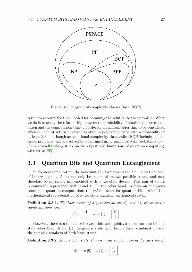
The complexity classes we have defined here form a hierarchical structure [4],which can be seen in Figure 2.4. As can be noted, PSPACE contains all of them,a quite surprising result. In fact, to date nobody has proven that P ( PSPACE,meaning that the full hierarchy may collapse in the future if P equals PSPACE. InFigure 2.5 we also show the relationship between P, NP and the complexity classesthat surround them, depending on the answer to the P versus NP problem. In theleft diagram, NP is represented by the circle, not by the space between NP-completeand P —that space corresponds to NP-intermediate, a class that will be explainedin Section 4.5—.
Now that we have formed the basis for the understanding of the main com-putational complexity classes, let us show where does some of the main problemsintroduced in the section dedicated to numerical semigroups fit into all this. For analmost complete and updated list of complexity classes, we refer to the vast databasefound in [5], result of the efforts of American theoretical computer scientist Scott

16 2. NUMERICAL SEMIGROUPS AND THE FROBENIUS PROBLEM
Figure 2.5: Diagram of P and NP-related complexity classes
Aaronson (b. 1981).
2.3 Computational Complexity of the Frobenius
Problem and the NSMP
In this section we are going to apply the background studied up to this point forproving that the Frobenius problem is in NP-hard. For that, first we are going toprove that the Boolean satisfiability problem is complete for the complexity class NP—i.e., that it is in NP, and is also hard for NP—. Then, we show that the numericalsemigroup membership problem is also in NP-complete. Finally, we prove that theFrobenius problem is hard for the class NP under Turing reductions to the NSMP.
Definition 2.3.1. The Boolean satisfiability problem, or SAT, is the problem of de-termining if there exists an interpretation for the binary variables x1, x2, . . . , xn thatsatisfies a given Boolean formula. In other words, given m clauses C1, C2, . . . , Cm,is the propositional logic formula C1 ∧ C2 ∧ · · · ∧ Cm satisfiable?
Definition 2.3.2. Let Π and Π′ be two decision problems, a polynomial-time many-one reduction from Π to Π′ is a polynomial-time algorithm for transforming inputsto problem Π into inputs to problem Π′, such that the transformed problem has thesame output as the original problem.
Theorem 2.3.3. (S. Cook – L. Levin) [37, 83] The Boolean satisfiability problemis in NP-complete.
Proof. In order to prove that the SAT problem is in NP-complete, we must de-mostrate two statements: first, that the SAT problem is in NP; second, that it is inNP-hard.
2.3. COMPUTATIONAL COMPLEXITY OF THE FP AND THE NSMP 17
It is easy to see that the first affirmation holds. Let C1, C2, . . . , Cm be a setof logical clauses involving the binary variables x1, x2, . . . , xn, a certificate for theveracity of all the clauses would be a vector in 0, 1n representing a truth assigne-ment. Naturally, a deterministic Turing machine that runs in polynomial time existsfor checking that our certificate makes every one of the clauses true.
The second part is customarily accomplished by showing that a well known NP-complete problem can be polynomially transformed to our problem; in this case,SAT. However, SAT was the first problem to be proven to be in NP-complete, howwas this accomplished? This result comes originally from the separated works ofAmerican-Canadian computer scientist and mathematician Stephen Cook (b. 1939)and Soviet-American computer scientist Leonid Levin (b. 1948), as both of themproved that every problem in NP can be reduced in polynomial time to SAT [37, 83].The proof we present here of Cook-Levin theorem is based on the ones found in [55]and [93].
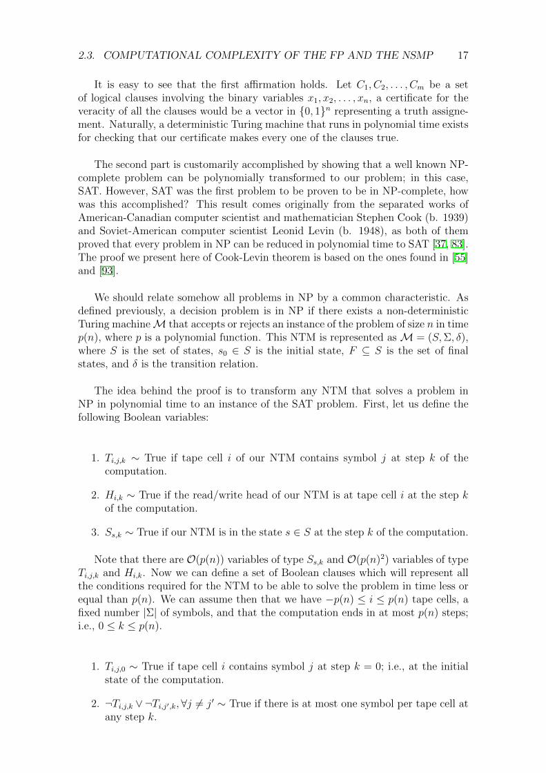
We should relate somehow all problems in NP by a common characteristic. Asdefined previously, a decision problem is in NP if there exists a non-deterministicTuring machineM that accepts or rejects an instance of the problem of size n in timep(n), where p is a polynomial function. This NTM is represented as M = (S,Σ, δ),where S is the set of states, s0 ∈ S is the initial state, F ⊆ S is the set of finalstates, and δ is the transition relation.
The idea behind the proof is to transform any NTM that solves a problem inNP in polynomial time to an instance of the SAT problem. First, let us define thefollowing Boolean variables:
1. Ti,j,k ∼ True if tape cell i of our NTM contains symbol j at step k of thecomputation.
2. Hi,k ∼ True if the read/write head of our NTM is at tape cell i at the step kof the computation.
3. Ss,k ∼ True if our NTM is in the state s ∈ S at the step k of the computation.
Note that there are O(p(n)) variables of type Ss,k and O(p(n)2) variables of typeTi,j,k and Hi,k. Now we can define a set of Boolean clauses which will represent allthe conditions required for the NTM to be able to solve the problem in time less orequal than p(n). We can assume then that we have −p(n) ≤ i ≤ p(n) tape cells, afixed number |Σ| of symbols, and that the computation ends in at most p(n) steps;i.e., 0 ≤ k ≤ p(n).
1. Ti,j,0 ∼ True if tape cell i contains symbol j at step k = 0; i.e., at the initialstate of the computation.
2. ¬Ti,j,k ∨¬Ti,j′,k,∀j 6= j′ ∼ True if there is at most one symbol per tape cell atany step k.

18 2. NUMERICAL SEMIGROUPS AND THE FROBENIUS PROBLEM
3.∨j∈Σ
Ti,j,k ∼ True if there is at least one symbol per tape cell at any step k.
4. Ss0,0 ∼ True if the initial state s0 ∈ S is the state of the computation at k = 0.
5. ¬Ss,k ∨ ¬Ss′,k,∀s 6= s′ ∼ True if our NTM is at only one state at any step k.
6. H0,0 ∼ True if the initial position of the read/write head of our NTM is intape cell i = 0.
7. ¬Hi,k ∨ ¬Hi′,k,∀i 6= i′ ∼ True if the read/write head of our NTM is at onlyone tape cell at any step k.
8. Ti,j,k ∧ Ti,j′,k+1 → Hi,j,∀j 6= j′ ∼ True if tape cell i remains unchanged unlessit has been written.
9. (Hi,k ∧Ss,k ∧ Ti,σ,k)→∨
((s,σ),(s′,σ′,d))∈δ
(Hi+d,k+1 ∧Ss′,k+1 ∧ Ti,σ′,k+1),∀k < p(n) ∼
True for all possible transitions at a computation step k ≤ p(n) when head isat position i.
10.∨
0≤k≤p(n)
∨f∈F
Sf,k ∼ True if the machine ends in one of the final states f ∈ F in
a step k ≤ p(n).
It is easy to see that there are O(1) clauses of type 4, 6 and 10; O(p(n)) clausesof type 1 and 5; O(p(n)2) clauses of type 2, 3, 8 and 9; and O(p(n)3) clauses oftype 7. This way, we can deduce that if there is an accepting computation for ourNTM on a certain input, then the conjunction of all previously defined clauses issatistifiable just by asigning the variables their corresponding value during the com-putation. Furthermore, if we solve the instance of SAT related to the conjunctionof those clauses, we can find a computation for M that follows the solution for theBoolean variables.
As there are O(p(n)) variables and O(p(n)3) clauses, the size of our SAT problemis O(log(p(n))p(n)3). Consequently, we have found a polynomial-time many-onereduction from any problem in NP to SAT, thus proving that SAT is in fact completefor the class NP.
Note that the previous theorem does not only show the existence of problems inNP-complete, but also states that if we find a polynomial time classical algorithm forthe SAT problem, we can also find a polynomial time algorithm for every problemin NP. However, this will unlikely happen, as it would imply that P = NP.
Now it is time to prove that the numerical semigroup membership problem isin NP-complete. A possible way of achieving this is seeing that, as said in Section2.2, NP-complete = NP ∩ NP-hard. In order to prove that a problem is in NP, itsuffices to show that a candidate solution is verifiable in polynomial time, which inthis case is trivial. For proving the NP-hardness of the NSMP, we must give firstthe following definitions, which can also be found in [59] and [93].

2.3. COMPUTATIONAL COMPLEXITY OF THE FP AND THE NSMP 19
Definition 2.3.4. Let Π and Π′ be two decision problems, a polynomial time Turingreduction from Π to Π′ is an algorithm ΛΠ which solves Π by using a hypotheticalsubroutine ΛΠ′ for solving Π′, such that, if ΛΠ′ were a polynomial time algorithmfor Π′ then ΛΠ would be a polynomial time algorithm for Π. In this context, we saythat the decision problem Π can be Turing reduced to Π′.
Proposition 2.3.5. Let Π be a decision problem, then Π is NP-hard if there existsan NP-complete decision problem Π′ such that Π′ can be Turing reduced to Π.
Definition 2.3.6. Let U , V and W be sets such that |U | = |V | = |W |, and T ⊆U × V ×W . Then, the 3-dimensonal matching problem, or 3DM, is the problem ofdetermining if there exists M ⊆ T with |M | = |U | such that
(u, v, w) 6= (u′, v′, w′) ⇐⇒ u 6= u′, v 6= v′, w 6= w′
for all (u, v, w), (u′, v′, w′) ∈M .
Definition 2.3.7. Let F = S1, . . . , Sn, where Si ⊆ S = u1, . . . , u3m and |Si| = 3for all i ∈ 1, . . . , n. Then, the 3-exact cover problem, or 3EC, is the problem ofdetermining if there is a subfamily of m subsets that covers S.
Definition 2.3.8. Let c1, . . . , cn ∈ Z≥0 and k ∈ Z≥0. Then, the 0-1 knapsackproblem, or 0-1KP, is the problem of determining if there exists S ⊆ 1, . . . , n suchthat ∑
j∈S
cj = k.
Theorem 2.3.9. The numerical semigroup membership problem is in NP-complete.
Proof. [93] It is trivial to see that 3DM, 3EC and 0-1KP are in NP. What remains tobe seen is that all of them are in NP-complete, and also that the NSMP transformsto one of them. First, we are going to prove that 3DM is in NP-complete, givinga polynomial transformation of an instance of SAT to an instance of 3DM. Letx1, . . . , xn be a set of binary variables and C1, . . . , Cm a set of Boolean clauses.We shall define an instance (U, V,W, T ) of 3DM such that M exists if and only ifF = C1 ∧ · · · ∧ Cm is satisfiable. Let
U = xji , xji : i = 1, . . . , n; j = 1, . . . ,m,
V = aji : i = 1, . . . , n; j = 1, . . . ,m∪ vj : j = 1, . . . ,m∪ cji : j = 1, . . . ,m, i = 1, . . . , n− 1,
W = bji : i = 1, . . . , n; j = 1, . . . ,m∪ wj : j = 1, . . . ,m∪ dji : j = 1, . . . ,m, i = 1, . . . , n− 1,
and

20 2. NUMERICAL SEMIGROUPS AND THE FROBENIUS PROBLEM
T = (aji , bji , x
ji ) : i = 1, . . . , n; j = 1, . . . ,m
∪ (aj+1i , bji , x
ji ) : i = 1, . . . , n; j = 1, . . . ,m
∪ (vj, wj, λj) : j = 1, . . . ,m;λ a literal (i.e. an atomic formula) of Cj∪ (cji , d
ji , λ
k) : i = 1, . . . , n− 1; j = 1, . . . ,m; k = 1, . . . ,m;λ a literal,
In order words, U contains a copy of each literal xi for each clause Cj; and V and Wcontain three kinds of nodes each. It follows that F is satisfiable if and only if thereexists a perfect matching M for (U, V,W, T ) (see [93] Theorem 15.7 for more details).
Second, we have to polynomially transform 3DM to 3EC, which happens if wedefine S = U ∪ V ∪W and F = a, b, c : (a, b, c) ∈ T. In fact, 3-dimensionalmatching is a special case of 3-exact cover.
Third, we have to polynomially transform 3EC to 0-1KP. Let us define
cj =∑ui∈Sj
(n+ 1)i+1
and
K =3m−1∑j=0
(n+ 1)j.
Then, it is easy to see that a subfamily F that covers u1, . . . , u3m exists if andonly if the instance c1, . . . , cn;K of 0-1KP thus defined has a solution.
Last, we have to polynomially transform 0-1KP to NSMP. Let M = 2n(n+1)K,if we define an instance d1, . . . , d2n;L of the NSMP, where
dj =
Mn+1 +M j + cj if j ≤ n
Mn+1 +M j−n otherwise
and
L = n ·Mn+1 +n∑j=1
M j +K,
then there exist integers y1, . . . , y2n ≥ 0 such that
2n∑j=1
djyj = L
if and only if there exist integers c1, . . . , cn ≥ 0 such that
n∑j=1
cjxj = K.
Although we have skipped some details of the validity of all previous transforma-tions for the sake of simplicity, a more exhaustive explanation can be found at [93](Chapter 15). Thus, we have transformed an instance of the SAT problem into aninstance of the NSMP, proving that the NSMP is complete for the class NP.

2.3. COMPUTATIONAL COMPLEXITY OF THE FP AND THE NSMP 21
Now that we have proved that the numerical semigroup membership problemis in NP-complete, it is time to finally prove that the Frobenius problem is in NP-hard. For that, we are going to define a polynomial algorithm ΛNSMP for solvingthe NSMP which uses as a subroutine an unknown algorithm ΛFP that solves theFrobenius problem. Thus, we prove that the NSMP can be Turing reduced to theFP. As the NSMP is in NP-complete, we shall conclude that the FP is in NP-hard.The proof we present here is adapted from the original result published by JorgeRamırez-Alfonsın in 1996 [97].
Let t ∈ Z≥0 and a1, . . . , an with gcd(a1, . . . , an) = 1. Then, the numericalsemigroup membership problem is defined as the problem of determining if thereexists a combination of non-negative integers λ1, . . . , λn ∈ Z≥0 such that
n∑i=1
λiai = t.
The algorithm ΛNSMP for the numerical semigroup membership problem will an-swer YES if the aforementioned combination λ1, . . . , λn exists for a certain inputt, a1, . . . , an —in other words, if t ∈ S0 = 〈a1, . . . , an〉—, and NO otherwise.
In the first place, ΛNSMP makes use of ΛFP and calculates f0 = f(S0). Then,three possible situations may appear: t > f0, t = f0 and t < f0. If t > f0, it is clearthat the answer is YES; if t = f0, then the answer is NO; if t < f0, then the answer isYES if and only if f2 < f1, with f1 and f2 defined as follows.
Let bi = 2ai for i = 1, . . . , n and let bn+1 = 2f0 + 1, then we define
S1 = 〈b1, . . . bn, bn+1〉
andf1 = f(S1).
Let bn+2 = f1 − 2t, we define
S2 = 〈b1, . . . bn, bn+1, bn+2〉
andf2 = f(S2).
Note that ΛNSMP makes use again of ΛFP for calculating f1 and f2. It remainsto be proven that the algorithm ΛNSMP answers correctly the NSMP. In order toachieve that, we need the following proposition.
Proposition 2.3.10. Let f0 and f1 be defined as in algorithm ΛNSMP, then f1 =4f0 + 1.
Proof. As f1 = f(S1), the proof needs only to show two statements: first, thatp > 4f0 + 1 implies p ∈ S1; second, that 4f0 + 1 /∈ S1.
Let p ∈ Z≥0 such that p > 4f0 + 1, then we define q as follows:

22 2. NUMERICAL SEMIGROUPS AND THE FROBENIUS PROBLEM
q =
p if p ≡ 0 mod 2
p− bn+1 if p ≡ 1 mod 2
It is easy to see that q > 2f0 in any case: in the first case,
q > 4f0 + 1 > 2f0,
and in the second case,
q = p− bn+1 > 4f0 + 1− (2f0 + 1) = 2f0.
As bn+1 = 2f0 + 1, then bn+1 ≡ 1 mod 2 and so q ≡ 0 mod 2 in both cases, whichimplies that q/2 > f0.
The last inequality implies that q/2 ∈ S0, which means that there exist someintegers α0, . . . , αn ∈ Z≥0 such that
q
2=
n∑i=1
αiai.
Following the definition of bi = 2ai we obtain that q ∈ S1, as
q =n∑i=1
αibi.
As S1 ⊂ S2, then q ∈ S2 and thus p ∈ S2, which proves the first statement.
The second statement can be proved by reductio ad absurdum. Let us supposethat 4f0 + 1 ∈ S1. This implies that there exist β1, . . . , βn, βn+1 ∈ Z≥0 such that
4f0 + 1 =n+1∑i=1
βibi.
As 4f0 + 1 ≡ 1 mod 2 and bi ≡ 0 mod 2 for i = 1, . . . , n (by definition ofbi = 2ai), then forcefully βn+1 6= 0. Let us suppose that βn+1 ≥ 2: then,
βn+1bn+1 ≥ 2bn+1 = 4f0 + 2 > 4f0 + 1,
which leads to a contradiction. It remains to be seen what happens if βn+1 = 1: weobtain
4f0 + 1 =n∑i=1
βibi + bn+1,
so
2f0 =n∑i=1
βibi,
and finally
f0 =n∑i=1
βiai,
which cannot be possible as f0 /∈ S0.
2.3. COMPUTATIONAL COMPLEXITY OF THE FP AND THE NSMP 23
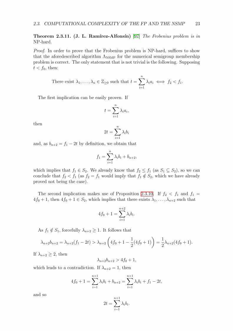
Theorem 2.3.11. (J. L. Ramırez-Alfonsın) [97] The Frobenius problem is inNP-hard.
Proof. In order to prove that the Frobenius problem is NP-hard, suffices to showthat the aforedescribed algorithm ΛNSMP for the numerical semigroup membershipproblem is correct. The only statement that is not trivial is the following. Supposingt < f0, then:
There exist λ1, . . . , λn ∈ Z≥0 such that t =n∑i=1
λiai ⇐⇒ f2 < f1.
The first implication can be easily proven. If
t =n∑i=1
λiai,
then
2t =n∑i=1
λibi
and, as bn+2 = f1 − 2t by definition, we obtain that
f1 =n∑i=1
λibi + bn+2,
which implies that f1 ∈ S2. We already know that f2 ≤ f1 (as S1 ⊆ S2), so we canconclude that f2 < f1 (as f2 = f1 would imply that f1 /∈ S2, which we have alreadyproved not being the case).
The second implication makes use of Proposition 2.3.10. If f2 < f1 and f1 =4f0 + 1, then 4f0 + 1 ∈ S2, which implies that there exists λ1, . . . , λn+2 such that
4f0 + 1 =n+2∑i=1
λibi.
As f1 /∈ S1, forcefully λn+2 ≥ 1. It follows that
λn+2bn+2 = λn+2(f1 − 2t) > λn+2
(4f0 + 1− 1
2(4f0 + 1)
)=
1
2λn+2(4f0 + 1).
If λn+2 ≥ 2, thenλn+2bn+2 > 4f0 + 1,
which leads to a contradiction. If λn+2 = 1, then
4f0 + 1 =n+1∑i=1
λibi + bn+2 =n+1∑i=1
λibi + f1 − 2t,
and so
2t =n+1∑i=1
λibi.

24 2. NUMERICAL SEMIGROUPS AND THE FROBENIUS PROBLEM
Even more, as bn+1 = 2f0 + 1 > 2t, then
2t =n∑i=1
λibi,
and finally
t =n∑i=1
λiai.
Please note that we have used an algorithm for solving the Frobenius problem inorder to prove that it is in NP-hard. However, the Frobenius problem was not statedas a decision problem, as its answer is an integer rather than a YES or NO output.These problems are known as function problems [62] and are usually redefined intoequivalent decision problems. In this case, the decision version of the Frobeniusproblem should be stated as follows:
Definition 2.3.12. Let S be a numerical semigroup and let k ∈ Z≥0, the decisionversion of the Frobenius problem answers YES if f(S) ≤ k and NO otherwise.
As explained in [62], an algorithm that solves a function problem can be polyno-mially transformed into an algorithm that solves the decision version of that sameproblem. In fact, function problems have its own complexity classes —for example,FP and FNP, which are the counterparts of P and NP—. However, FP and FNPare seldom used when a decision version for a function problem can be defined, asin this case.
In addition, the numerical semigroup membership problem of a certain t ∈ Z≥0
with respect to a numerical semigroup S can be trivially Turing reduced to theproblem of finding the Sylvester denumerant d(t, S), as d(t, S) ≥ 1 ⇐⇒ t ∈ S.Thus, we can obtain the following result:
Corollary 2.3.13. The Sylvester denumerant problem is in NP-hard.

3
Quantum Computation
“I make up the rules, I’m allowed to do that.”– Richard P. Feynman, Simulating Physics with Computers
“Someday you will be old enough to start reading fairy tales again.”– C. S. Lewis, The Chronicles of Narnia
3.1 Introduction
The origins of quantum computation date back to 1980, when American physicistPaul Benioff (b. 1930) described a computing model defined by quantum mechanicalHamiltonians [19]. Later that year, Russian mathematician Yuri Manin gave a firstidea on how to simulate a quantum system with a computer governed by quantummechanics [86]. Both of them laid the groundwork for two of the basic componentsof quantum computing: quantum Turing machines and quantum computers [91].
Two years later, American theoretical physicist Richard Feynman (1918 – 1988)talked in one of his most seminal papers about the problems of simulating physicswith a classical computer [52], and introduced independently a quantum model ofcomputation. He stated that, being the world quantum mechanical, the inherentdifficulty within the possibility of exactly replicating the behavior of nature is re-lated to the problem of simulating quantum physics. This way, the most importantrule defined by Feynman deals with the computational complexity at the time of ef-ficiently simulating a quantum system. If one doubles the dimensions of the system,it would be ideal that the size of the computational resources needed for this taskalso double in the worst case, instead of experimenting an exponential growth.
Feynman also stated the underlying limitations that appear when it comes tosimulate the probabilities of a physical system. Instead of calculating the proba-bilities of such a system, which he proved to be impossible, he proposed that thecomputer itself should have a probabilistic nature. To this new kind of machine hegave the name of quantum computer, and stated that it had a distinct essence thanthe well-known Turing machines. He also noted that with one of them it shouldbe possible to simulate correctly any quantum system, and the physical world it-self. Feynman asked himself if it would be possible to define a universal quantum
25
26 3. QUANTUM COMPUTATION
computer, capable of modeling all possible quantum systems and detached from thepossible problems that originate from its physical implementation, in the same waythat a classical one is.
3.2 Quantum Turing Machines
Although the credit for introducing the concept of a universal quantum computergoes to Richard Feynman, it was British physicist David Deutsch (b. 1953) the firstto properly describe, generalize and formalize it [41]. Supported in the works byFeynman, Manin and Benioff, he also introduced the concept of quantum Turingmachine, which we proceed to define:
Definition 3.2.1. A quantum Turing machine M, or QTM, is defined by a tripleM = (S,Σ, δ), where the set of states S is replaced by the pure and mixed states ofa Hilbert space, the alphabet Σ is finite, and the transition function δ is substitutedfor a set of unitary transformations which are automorphisms of S.
This definition is rather informal and leaves out many important details. In fact,the study of quantum Turing machines is quite intricate, as many of its ingredients—such as the head position— can exist in a superposition of classical states [15].Fortunately, an equivalent and much more friendly paradigm of computation calledthe quantum circuit model exists, and will be explained later on in this chapter alongwith all its details. Nevertheless, the reader interested in the complete and originaldefinition of quantum Turing machines and all of their characteristics, can refer tothe seminal papers where they were first outlined and formalized: [41], [42] and[22]. Besides, a quantum Turing machine can also be seen as a probabilistic Turingmachine that obeys the rules of quantum probability instead of classical probability[106].
Definition 3.2.2. The complexity class BQP, which stands for bounded-error quan-tum polynomial-time, contains all decision problems that can be solved in polynomialtime by a quantum Turing machine with error probability bounded by 1/3 for all in-puts.
The latter class is usually taken as a reference for representing the power of quan-tum computers. Thanks to [22] and [41], we already know that BQP ⊆ PSPACEand that BPP ⊆ BQP. However, at the present time there is no known relationshipbetween NP and BQP, except that P is inside their intersection. There is a strongbelief that NP * BQP; consequently, a polynomial-time quantum algorithm for anNP-complete problem would be surprising, as it would violate this conjecture. Sofar, we can update our previous complexity class diagram with this new class, asseen in Figure 3.2. A problem that is not known to be in BPP —or in P— is thefactoring problem, but we already know thanks to Peter W. Shor a polynomial-timealgorithm for this problem that runs on a quantum computer [105]. This algorithm,among many others, will be thoroughly explained in the next chapter.
It can be deduced from the definition of the complexity class BQP that the innernature of quantum computation is probabilistic. In order to measure the perfor-mance of a quantum algorithm that solves a certain problem, we do not usually
3.3. QUANTUM BITS AND QUANTUM ENTANGLEMENT 27
Figure 3.1: Diagram of complexity classes (incl. BQP)
take into account the time needed for obtaining the solution to that problem. Whatwe do is to study the relationship between the probability of obtaining a correct so-lution and the computation time. In order for a quantum algorithm to be consideredefficient, it must return a correct solution in polynomial time with a probability ofat least 2/3 —although an additional complexity class, called EQP, includes all de-cision problems that are solved by quantum Turing machines with probability 1—.For a groundbreaking study on the algorithmic limitations of quantum computing,we refer to [20].
3.3 Quantum Bits and Quantum Entanglement
In classical computation, the basic unit of information is the bit —a portmanteauof binary digit—. A bit can only be in one of its two possible states, and maytherefore be physically implemented with a two-state device. This pair of valuesis commonly represented with 0 and 1. On the other hand, we have an analogousconcept in quantum computation: the qubit —short for quantum bit— which is amathematical representation of a two-state quantum-mechanical system.
Definition 3.3.1. The basis states of a quantum bit are |0〉 and |1〉, whose vectorrepresentations are:
|0〉 =
[10
]and |1〉 =
[01
]However, there is a difference between bits and qubits, a qubit can also be in a
state other than |0〉 and |1〉. Its generic state is, in fact, a linear combination overthe complex numbers of both basis states.
Definition 3.3.2. A pure qubit state |ψ〉 is a linear combination of the basis states,
|ψ〉 = α |0〉+ β |1〉 =
[αβ
]

28 3. QUANTUM COMPUTATION
where α, β ∈ C are called the amplitudes of the state and for which the constraint
|α|2 + |β|2 = 1
holds.
Remark: Note that we have introduced a new notation, |ψ〉, termed ket, for de-scribing a quantum state. This notation is part of the bra-ket notation, also namedDirac notation in honor of English theoretical physicist Paul Dirac (1902 – 1984),who first introduced it in 1939 [45]. Alternatively, we will also use 〈ψ|, called bra,to describe |ψ〉∗ (the Hermitian adjoint of |ψ〉).
Thus, we can say that |0〉 and |1〉 form an orthonormal C-basis of C2 and thatthe state of a single-qubit system |ψ〉 is a unit vector of C2 (i.e., |ψ〉 ∈ C2 with|| |ψ〉|| = 1). From now on, the basis formed by |0〉 and |1〉 will be called thecomputational basis of a qubit. Nevertheless, there are other commonly used basisfor the states of a quantum bit. Another example that will come in handy later,known as the Hadamard basis in honor of French mathematician Jacques Hadamard(1865 – 1963), is defined by
|+〉 =1√2
(|0〉+ |1〉) =1√2
[11
]and
|−〉 =1√2
(|0〉 − |1〉) =1√2
[1−1
].
It is easy to see that |+〉 and |−〉 also form an orthonormal C-basis of C2, and thatour generic qubit |ψ〉 = α |0〉+ β |1〉 can be seen as
|ψ〉 =α + β√
2|+〉+
α− β√2|−〉 .
We know that qubits exist in nature thanks to the Stern-Gerlacht experiment,first conducted by German physicists Otto Stern (1888 – 1969) and Walther Gerlach(1889 – 1979) in 1922 [56]. A possible geometrical representation of the states ofa single-qubit system, known as the Bloch sphere [24, 91] —see Figure 3.2—, leanson the fact that a generic qubit α |0〉 + β |1〉 with |α|2 + |β|2 = 1 can be repre-sented uniquely as a point (θ, φ) of the unit 2-sphere, with the north and southpoles typically chosen to correspond to the standard basis vectors |0〉 and |1〉, andwhere α = cos(θ/2) and β = eiφ sin(θ/2). Thus, we can see a qubit system asa unitary vector, and any transformation we would want to apply to it must pre-serve its norm. We shall explain these transformations in Section 3.4, but for now letus focus on what happens when we try to measure the state of a single-qubit system.
One of the key features that makes a quantum computer differ dramaticallyfrom its classical counterpart is the process of measuring the state of a quantumbit. A measurement, also called observation, of a generic single-qubit state |ψ〉 =α |0〉 + β |1〉 yields a result from the orthonormal basis, depending on the valuesof α and β. However, the measurement process inevitably disturbs |ψ〉, forcing itto collapse to either |0〉 or |1〉 and thus generally making impossible the task of

3.3. QUANTUM BITS AND QUANTUM ENTANGLEMENT 29
Figure 3.2: Bloch sphere1
finding out the actual values of α and β. This collapse to either |0〉 or |1〉 is non-deterministic and is ruled by the given probabilities |α|2 and |β|2 respectively. Itwill be shown in Section 3.4 how to change these probabilities without violating theunitarity constraint. But first, let us explain some concepts needed to understandhow multiple-qubit systems behave.
Definition 3.3.3. Let V and W be vector spaces of dimensions n and m respectively.The tensor product of V and W , denoted by V ⊗W , is an nm-dimensional vectorspace whose elements are linear combinations of tensor products v⊗w satisfying thesubsequent properties:
• z(v ⊗ w) = (zv)⊗ w = v ⊗ (zw)
• (v1 + v2)⊗ w = (v1 ⊗ w) + (v2 ⊗ w)
• v ⊗ (w1 + w2) = (v ⊗ w1) + (v ⊗ w2)
where z ∈ C, v, v1, v2 ∈ V and w,w1, w2 ∈ W .
A related definition that will come to use in Section 3.4 is the concept of tensorproduct between linear operators.
Definition 3.3.4. Let A and B be linear operators defined on V and W respectively,then the linear operator A⊗B operating on V ⊗W is defined as
(A⊗B)(v ⊗ w) = Av ⊗Bw
with v ∈ V and w ∈ W , and has the following matrix representation with respect tothe canonical base:
A⊗B =
a11B a12B · · · a1nBa21B a22B · · · a2nB
......
. . ....
an1B an2B · · · annB
1Credit: Glosser.ca (CC BY-SA 3.0)

30 3. QUANTUM COMPUTATION
where A and B are n × n and m ×m matrices respectively that correspond to thematrix representations of the linear operators A and B with respect to the canon-ical base. Note that we can conclude that the matrix representation of A ⊗ B hasdimension nm× nm.
By means of an example on how the matrix representations of the tensor productsof linear operators are calculated, let
A =
[1 −1−2 0
]and B =
1 0 00 2 00 0 3
be two linear operations defined on R2 and R3 respectively. Then, their tensorproduct is calculated as follows:
A⊗B =
[1 −1−2 0
]⊗
1 0 00 2 00 0 3
=
1 0 0 −1 0 00 2 0 0 −2 00 0 3 0 0 −3−2 0 0 0 0 0
0 −4 0 0 0 00 0 −6 0 0 0
where A⊗B is a linear operator defined on R6.
The tensor product we have thus defined can also be extended to vectors andnon-square matrices, and will be useful at the time of calculating the basis statesof a quantum system with more than one qubit. For instance, if |0〉 and |1〉 are thebasis states of a quantum bit, the tensor product |1〉 ⊗ |0〉 will be given by:
|1〉 ⊗ |0〉 =
[01
]⊗[
10
]=
0010
Before continuing with the possible states of a multiple qubit system, let us
introduce some notation. In a classical computer, we represent an integer a ∈ Z≥0
such that a < 2n —i.e., such that it can be described with n bits— with the base-2numeral system:
a =n−1∑l=0
al2l
where al ∈ 0, 1 are the binary digits of a. In a quantum computer, we can alsorepresent an integer a < 2n with n qubits as follows:
|a〉n = |an−1 · · · a1a0〉 =n−1⊗l=0
|al〉
Thus, for example, number 29 can be represented with 5 qubits (as 29 < 25) likethis:
|29〉5 = |11101〉 = |1〉 ⊗ |1〉 ⊗ |1〉 ⊗ |0〉 ⊗ |1〉 .

3.3. QUANTUM BITS AND QUANTUM ENTANGLEMENT 31
From now on, the notation |ψ〉n will imply that we are describing a n-qubitsystem —where n ≥ 2— instead of a single-qubit one, which will remain to beindicated with the absence of a subindex. We will also make use sometimes ofthe notation |uv〉 to describe the tensor product |u〉 ⊗ |v〉 of two basis states, withu, v ∈ 0, 1. Now that we know what |ψ〉n and |a〉n really mean, we are finally inthe position to begin studying the possible states of a multiple qubit system.
Definition 3.3.5. The basis states of a two-qubit system are the tensor products ofthe basis states of a single-qubit system:
|0〉2 = |00〉 = |0〉 ⊗ |0〉 =
[10
]⊗[
10
]=
1000
|1〉2 = |01〉 = |0〉 ⊗ |1〉 =
[10
]⊗[
01
]=
0100
|2〉2 = |10〉 = |1〉 ⊗ |0〉 =
[01
]⊗[
10
]=
0010
|3〉2 = |11〉 = |1〉 ⊗ |1〉 =
[01
]⊗[
01
]=
0001
We shall see what happens when two qubits interact. The generic state of two
different single-qubit systems, described independently, can be represented as
|ψ0〉 = α |0〉+ β |1〉 = α
[10
]+ β
[01
]=
[αβ
]and
|ψ1〉 = γ |0〉+ δ |1〉 = γ
[10
]+ δ
[01
]=
[γδ
],
where |α|2 + |β|2 = 1 and |γ|2 + |δ|2 = 1. This means that the state of this 2-qubitsystem should be described as the tensor product of both of them:
|ψ0〉 ⊗ |ψ1〉 =
[αβ
]⊗[γδ
]=
αγαδβγβδ
.On the other hand, if we want to describe a generic 2-qubit system |ψ〉2 with the
basis states defined in 3.3.5, we would have
|ψ〉2 = α0
1000
+ α1
0100
+ α2
0010
+ α3
0001
=
α0
α1
α2
α3
,
32 3. QUANTUM COMPUTATION
where
|α0|2 + |α1|2 + |α2|2 + |α3|2 = 1
must hold —remember that any quantum state must be described as a unitary vec-tor—.
Note that a new constraint has arisen. If our generic two-qubit system describedby |ψ〉2 is to be decomposed in two single-qubit states (i.e., |ψ〉2 = |ψ0〉⊗|ψ1〉), thenα0 = αγ, α1 = αδ, α2 = βγ and α3 = βδ. It is easy to see that the equality α0α3 =α1α2 is imposed; however, there exists a physical phenomenon called quantumentanglement which implies that the quantum state of each one of the particles ofa two-qubit system may not be described independently. In other words, it is notmandatory that the constraint α0α3 = α1α2 holds in a generic two-qubit system,which leads us to the subsequent definitions:
Definition 3.3.6. A two-qubit general state is a linear combination of the basisstates of a two-qubit system:
|ψ〉 = α0 |0〉2 + α1 |1〉2 + α2 |2〉2 + α3 |3〉2holding the following constraint:
|α0|2 + |α1|2 + |α2|2 + |α3|2 = 1
Definition 3.3.7. A two-qubit general state |ψ〉2 is called mixed or entangled if theredoes not exist two one-qubit states |ψ0〉 and |ψ1〉 such that |ψ〉2 = |ψ0〉 ⊗ |ψ1〉 (i.e.,if it cannot be tensor-factorized).
Quantum entanglement was first observed in nature in 1935, and in early days itwas known as the EPR or Einstein–Podolsky–Rosen paradox. It was first studied byGerman-born theoretical physicist Albert Einstein (1879 – 1955) and his colleaguesBoris Podolsky (1896 – 1966) and Nathan Rosen (1909 – 1995) [47], and later byAustrian physicist Erwin Schrodinger (1887 – 1961) [104]. The role and importanceof quantum entanglement in quantum algorithms operating on pure states and inquantum computational speed-up was extensively discussed by Richard Jozsa andNoah Linden in [70].
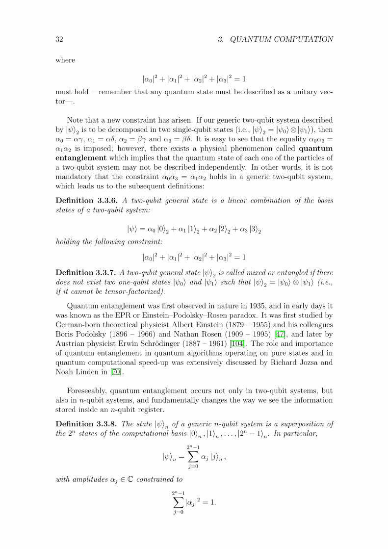
Foreseeably, quantum entanglement occurs not only in two-qubit systems, butalso in n-qubit systems, and fundamentally changes the way we see the informationstored inside an n-qubit register.
Definition 3.3.8. The state |ψ〉n of a generic n-qubit system is a superposition ofthe 2n states of the computational basis |0〉n , |1〉n , . . . , |2n − 1〉n. In particular,
|ψ〉n =2n−1∑j=0
αj |j〉n ,
with amplitudes αj ∈ C constrained to
2n−1∑j=0
|αj|2 = 1.

3.3. QUANTUM BITS AND QUANTUM ENTANGLEMENT 33
This can be seen as an obvious advantage with respect to classical computation.In a conventional computer we can store one but only one integer between 0 and2n − 1 inside a n-bit register, which can be seen as a probability distribution be-tween all possible integers where the integer we have stored has probability 1 andthe rest have 0. In a quantum register, the probability can be distributed betweenall those integers instead of having just one possibility when it comes to read theregister. Even more, if we are to simulate this quantum behavior with a classicalcomputer, we would need 2n registers of n bits, instead of a single n-qubit registeras in the quantum case. This is precisely one of the benefits of quantum computingthat Richard Feynman foretold in his paper [52].
Analogously to the single-qubit case, observing an n-qubit system unavoidablyinterferes with |ψ〉n and impels it to collapse in one of the vectors of the computa-tional basis (i.e., in |j〉n with 0 ≤ j < 2n). This collapse is again non-deterministicand is governed by the probability distribution given by |αj|2. Thus, all the infor-mation that may have been stored in the amplitudes αj is inevitably lost after themeasurement process.
By way of illustration, let us suppose that we have the following 3-qubit quantumsystem:
|ψ〉3 =1
2|1〉3 +
1
2|3〉3 +
1
2|5〉3 +
1
2|7〉3 .
Then, if we measure this system, we will obtain with identical probability one of thesepossible outcomes: 1, 3, 5 or 7. Additionally, it is interesting to see the behavior ofa quantum system if, rather than measuring all qubits at once, we measure themone by one. Our previous quantum system can be seen as
|ψ〉3 =1
2|001〉+
1
2|011〉+
1
2|101〉+
1
2|111〉 .
But also as
|ψ〉3 =1√2|0〉 ⊗
( 1√2|01〉+
1√2|11〉
)+
1√2|1〉 ⊗
( 1√2|01〉+
1√2|11〉
)or as
|ψ〉3 =( 1√
2|0〉+
1√2|1〉)⊗( 1√
2|01〉+
1√2|11〉
).
If we measure the first qubit, we have the same probability of obtaining 0 or 1.However, as the measurement collapses the state of the qubit, the two remainingqubits will be forced to be in a state that is somewhat linked to the one we haveobtained for the first qubit —i.e., the part that is tensored with the result we obtainfor the first qubit—. Let us suppose that by measuring the first qubit, we haveobtained a 1. Then, our 3-qubit system has collapsed to
|ψ〉3 = |1〉 ⊗( 1√
2|01〉+
1√2|11〉
),
which can also be seen as
|ψ〉3 = |1〉 ⊗( 1√
2|0〉+
1√2|1〉)⊗ |1〉 .

34 3. QUANTUM COMPUTATION
Note that the third qubit is already in one of the states of the computationalbasis, which means that, if we measure it right now, we will certainly obtain thevalue 1. The only remaining qubit that is not in the computational basis is thesecond one. Looking at the current state of our system, it is easy to see that wehave the same probability of obtaining 0 or 1 by measuring it, which means that wewill obtain 5 or 7.
It is of interest to see if the result we obtain from one of the qubits will conditionthe possible values for the remaining qubits. Let
|ψ〉2 =1√2
(|0〉 ⊗ |0〉) +1√2
(|1〉 ⊗ |1〉)
be one of the four possible Bell states [18, 91], named after Northern Irish physicistJohn Stewart Bell (1928 – 1990). This state is composed of two entangled qubits—they cannot be described as two single-qubit states—. If we measure the secondqubit, we have the same probability of obtaining 0 or 1. However, if we first measurethe first qubit, and obtain 1, then the state of the second qubit will collapse —with-out having observed it— to 1, as the value 1 for the second qubit is only tensoredwith the value 1 of the first qubit. Thus, the result we obtain from a qubit or aset of qubits can be conditioned by the order in which we proceed to measure therest of qubits. As will be seen in Chapters 4 and 5, the order in which we choose toread the members of a quantum register is one of the most important aspects of aquantum algorithm.
Another set of operations between qubits that are of great value are the innerand outer products, which we proceed to define.
Definition 3.3.9. Let |ψ0〉n and |ψ1〉n be two n-qubit systems, the inner product of|ψ0〉n and |ψ1〉n is defined as usual by
〈ψ0|ψ1〉n = |ψ0〉∗n |ψ1〉n
The inner product has the following properties:
• 〈ψ0|ψ1〉n = 〈ψ1|ψ0〉∗n
• 〈ψ0|(a |ψ1〉+ b |ψ2〉)〉n = a 〈ψ0|ψ1〉n + b 〈ψ0|ψ2〉n
• 〈ψ|ψ〉n = || |ψ〉n ||2
Definition 3.3.10. Let |ψ0〉n and |ψ1〉n be two n-qubit systems, the outer productof |ψ0〉n and |ψ1〉n is defined by
|ψ0〉 〈ψ1|n = |ψ0〉n |ψ1〉∗n
For example, let
|ψ0〉 = α |0〉+ β |1〉 =
[αβ
]

3.4. QUANTUM CIRCUITS 35
and
|ψ1〉 = γ |0〉+ δ |1〉 =
[γδ
]be two generic single-qubit systems, then the matrix representations of the innerand outer product between |ψ0〉 and |ψ1〉 are calculated as follows:
〈ψ0|ψ1〉 =[α∗ β∗
] [ γδ
]= α∗γ + β∗δ,
|ψ0〉 〈ψ1| =[αβ
] [γ∗ δ∗
]=
[αγ∗ αδ∗
βγ∗ βδ∗
].
Note that 〈ψ|ψ〉 = 1 for any quantum state |ψ〉.
3.4 Quantum Circuits
The language of quantum circuits is a model of computation which is equivalentto quantum Turing machines and to universal quantum computers [115]. Currently,it is the more extensively used when it comes to describe an algorithm that runson a quantum machine, and draws upon a sequence of register measurements —asdescribed in Section 3.3— and discrete transformations —which will be explainedin this section, as promised—. This is mainly due because all its elements can betreated as classical, with the sole exception of the information that is going throughthe wires.
First, we shall see what kind of transformations can be applied to the state ofan n-qubit system. As a quantum state is always represented by a unit vector, weneed the most general operator that preserves this property and the dimension ofthe vector.
Definition 3.4.1. A matrix A ∈MC(n) is unitary if
A∗A = AA∗ = I
where I is the identity matrix and A∗ is the Hermitian adjoint of A.
Definition 3.4.2. The unitary group of degree n, denoted by UC(n), is the group ofn× n unitary matrices, with matrix multiplication as the group operation.
Proposition 3.4.3. Let A ∈ UC(n) be a unitary matrix and let x ∈ Cn be a unitvector, then Ax ∈ Cn is also a unit vector.
In this context, a unitary transformation acting on n-qubits is called an n-qubitquantum gate, and can be represented by a unitary matrix. Let us expand thisconcept and its physical implications.
Definition 3.4.4. A quantum gate that operates on a space of one qubit is repre-sented by a unitary matrix A ∈ UC(2). More generally, a quantum gate acting onan n-qubit system is represented by a unitary matrix A ∈ UC(2n).

36 3. QUANTUM COMPUTATION
Please note that quantum gates necessarily have the same number of inputs andoutputs, as opposed to classical logic gates. From now on, all quantum gates will berepresented with a bold symbol, in order to differenciate them from mere matrices.We will show the most frequently used quantum gates as examples, and variousresults that simplify in a dramatic way the difficulty of implementing physically anyquantum gate.
Definition 3.4.5. The Hadamard gate is a single-qubit gate with the following ma-trix representation:
H =1√2
[1 11 −1
]which is unitary.
The circuit representation of the Hadamard gate is
|ψ0〉 H |ψ1〉
and, applied to each of the basis states, it has the following effect:
H : |j〉 → 1√2
(|0〉+ (−1)j |1〉
).
As will be seen in Chapter 4, the Hadamard transformation is one of the mostimportant quantum gates, since it is the basis of the majority of quantum algorithmsdeveloped to date. Its importance settles in the role it has at the time of generatingall possible basis states, all of them with the same amplitude, inside a quantumregister. Let us suppose that we have a qubit whose quantum state is |ψ0〉 =α |0〉+ β |1〉, where |α|2 + |β|2 = 1. Then, the state of this single-qubit system afterapplying the Hadamard gate to it is:
H |ψ0〉 =1√2
[1 11 −1
] [αβ
]=
1√2
[α + βα− β
]=α + β√
2|0〉+
α− β√2|1〉
Let us suppose now that, rather than having a generic state, we have the basisstate |ψ0〉 = |0〉 in our one-qubit system. In that case, the result of applying theHadamard gate will be as follows:
H |0〉 =1√2
[1 11 −1
] [10
]=
1√2
[11
]=
1√2|0〉+
1√2|1〉
As can be appreciated, we have transformed a basis state, |0〉, into a linearcombination of the two basis states, |0〉 y |1〉, with identical amplitudes. If wemeasure the qubit at this moment, we will obtain with equal probability one of thetwo possible basis states. That said, what will happen if, rather than having a singlequantum state, we have a n-qubit quantum system, all of them also in their basisstate |0〉?
H⊗n |0〉n =1√2n
[1 11 −1
]⊗n [10
]⊗n=
1√2n
[11
]⊗n=
1√2n
2n−1∑j=0
|j〉n

3.4. QUANTUM CIRCUITS 37
What we have obtained is a superposition of all basis states of the system withidentical probability. In other words, if we measure our n-qubit register right now,we will obtain a certain integer j ∈ 0, . . . , 2n − 1 with probability 1/2n.
Definition 3.4.6. The Pauli gates are single-qubit gates with the following matrices:
X =
[0 11 0
]Y =
[0 −ii 0
]Z =
[1 00 −1
]which are unitary, but also Hermitian.
The Pauli matrices have the following effect on the basis states:
X : |j〉 → |1⊕ j〉
Y : |j〉 → (−i)j |1⊕ j〉
Z : |j〉 → (−1)j |j〉The three previous quantum gates are named after Austrian-born Swiss and
American theoretical physicist Wolfgang Pauli (1900 — 1958). The three of them,along with the identity matrix I, form a basis for the vector space of 2 × 2 Hermitianmatrices multiplied by real coefficients. However, all previously defined quantumgates have their limitations. In fact, quantum gates that are the direct product ofsingle-qubit gates cannot produce entanglement.
Definition 3.4.7. The CNOT gate, which stands for controlled-not, is a two-qubitquantum gate with the following matrix representation:
CNOT =
1 0 0 00 1 0 00 0 0 10 0 1 0
Applied to a two-qubit basis state, the CNOT gate has the next effect:
CNOT : |i〉 ⊗ |j〉 → |i〉 ⊗ |i⊕ j〉 .
TheCNOT gate is another one of the key quantum gates, as it can be used to entangleand disentangle Bell states. In fact, it is the most simple gate that produces quantumentanglement. For example, let
|ψ〉2 =1√2
(|0〉2 + |2〉2)
be a separable quantum state (as |ψ〉2 = |+〉 ⊗ |0〉). If we apply the CNOT gate toit, we obtain

38 3. QUANTUM COMPUTATION
|ψ′〉2 = CNOT (|ψ〉2)
=1√2
(CNOT (|0〉 ⊗ |0〉) +CNOT (|1〉 ⊗ |0〉)
)=
1√2
(|0〉 ⊗ |0〉+ |1〉 ⊗ |1〉) ,
which is one of the entangled Bell states.
Theorem 3.4.8. [46, 15] Let A ∈MC(2n) be a n-qubit gate, then it can be expressedas a finite number of tensor products of single-bit gates Mi ∈ MC(2) and the two-qubit CNOT gate.
The previous result imply that every unitary transformation on an n-qubit sys-tem can be implemented physically using only single-qubit gates and theCNOT gate.In other words, single-qubit gates and the CNOT gates form a set of universal gates.In fact, the most interesting result that links quantum entanglement and quantumcomputing performance over classical computation is the following:
Theorem 3.4.9. (Gottesman–Knill) A quantum algorithm that starts in a com-putational basis state and does not feature quantum entanglement can be simulatedin polynomial time by a probabilistic classical computer [60].
Thus, we have explained the main notions needed for the correct comprehensionof the rest of this doctoral thesis: a quantum circuit algorithm will consist in a setof transformations of two different types, observations and unitary transformations,to a n-qubit register. But before proceeding with the explanation of some of themost important quantum algorithms to date, let us describe a different model ofquantum computing to that of quantum circuits.
3.5 Adiabatic Quantum Computing
Adiabatic quantum computing, or AQC, is an alternative model of quantumcomputing which apparently does not have much in common with quantum circuits.Nevertheless, both models are equivalent, as will be mentioned later, and thus adi-abatic quantum computers are also tantamount to quantum Turing machines.
As hinted in the previous section —it will be fully explained in Chapter 4— aquantum circuit obtains an answer for a certain problem as a result of a succesionof quantum gates and register observations, in a process that has a discrete nature.On the other hand, the behavior of an adiabatic quantum computer is essentialycontinuous —in fact, quantum circuits and adiabatic quantum computers are oftenrespectively labelled as digital and analogic quantum computers— and is governedby the adiabatic theorem, a concept in quantum mechanics developed by Germanphysicist and mathematician Max Born (1882 – 1970) and Soviet physicist VladimirFock (1898 – 1974), and first stated in 1928 [27]. Although the original paper is inGerman, extensive English-written studies on the adiabatic theorem can be found in[72, 88, 99]. Before proceeding with the adiabatic theorem, we need a few definitions.
3.5. ADIABATIC QUANTUM COMPUTING 39
Definition 3.5.1. A Hamiltonian, denoted by H, is an operator corresponding tothe total energy of a quantum system. Its spectrum —the set of its eigenvalues— isthe set of all possible outcomes that one could obtain when measuring the energy ofsuch a system.
Definition 3.5.2. The ground state of a quantum system defined by a HamiltonianH is the eigenvector of the smallest eigenvalue of H. In the same way, its firstexcited state is the eigenvector of the second smallest eigenvalue of H.
We are now in position to understand the Schrodinger equation [103, 104], amathematical equation result of the research of Erwin Schrodinger, which tells ushow a quantum system evolves over time:
i~d
dt|ψ(t)〉 = H(t) |ψ(t)〉 .
Where |ψ(t)〉 is the time-dependent quantum state of the system.
Thus, the adiabatic theorem can be informally stated as:
“A physical system remains in its ground state if a given perturbation is actingon it slowly enough and if there is a gap between the associated eigenvalue and therest of the Hamiltonian’s spectrum.”
Although the original formulation of the adiabatic theorem is due to Born andFock, the first proper proof of this result [9] was made by Japanese mathematicianTosio Kato (1917 – 1999), and can be found in [72].
The main idea behind adiabatic quantum computation is to define a Hamiltonianwith respect to time in such a way that its initial ground state would be easy tocalculate, and its final ground state would be the solution to a certain problem. Thisprocess, called quantum adiabatic evolution, can be seen as the following equation:
H(t) = Γ(t)HI + Λ(t)HF
where HI —the initial Hamiltonian— has a known ground state and HF —the finalHamiltonian— has an unknown one that encodes the solution to our problem; t goesfrom 0 to T ; Γ(t) decreases from 1 to 0; and Λ(t) increases from 0 to 1 monotonicallywith time. A typical case is when Γ(t) = s(t) and Λ(t) = 1−s(t) with s(t) = 1−t/T ,which gives us:
H(t) = s(t)HI + (1− s(t))HF
Early works on the subject tried to replicate the performance of simulated an-nealing, a probabilistic technique for approximating the global minimum of a certainobjective function —see [74] for more details—, in a quantum manner —i.e., takingadvantage of tunneling and quantum fluctuations instead of thermal fluctuations inorder to escape from local minima—. In these works, however, where it was calledquantum annealing —see, for example, the seminal paper by Tadashi Kadowaki andHidetoshi Nishimori [71]—, the main idea was to simulate this quantum behaviorclassically. The first experimental approach to quantum annealing came in 1999

40 3. QUANTUM COMPUTATION
usign a disordered quantum ferromagnet [32, 33], a result that hinted a possiblequantum model of computation based on the adiabatic theorem.
The first quantum adiabatic algorithm, which solves certain instances of a combi-natorial optimization problem —more concretely, the Boolean satisfiability problem,which we have already proven to be complete for NP—, was given by Edward Farhi,Jeffrey Goldstone, Sam Gutmann and Michael Sipser in 2000 [50, 49]. Afterwards,Wim van Dam, Michele Mosca and Umesh Vazirani studied in [112] the complexityof this algorithm, while also giving an adiabatic version of Grover’s database searchthat also offers a quadratic speedup over the classical search algorithm.
Up to this point, the Hamiltonians involved in this kind of optimization prob-lems share a common factor: they are stoquastic —meaning that all its off-diagonalmatrix elements in the standard basis are real and non-positive—. However, thegeneralization of the model of adiabatic quantum computing that depends also onnon-stoquastic Hamiltonians was proven to be equivalent to the quantum circuitmodel [8, 89] and thus to quantum Turing machines. This larger model is capableof solving any Turing-computable problem, instead of just the typically NP-hardcombinatorial optimization problems associated with quantum annealing (see [87],which in turn cites [102]). In fact, it can polynomially simulate any quantum algo-rithm based on the quantum circuit model [8].
A problem associated with adiabatic quantum computing is the set of difficultiesthat arise at the time of measuring the performance of an adiabatic quantum algo-rithm. The most important deals with the computational time needed for evolvingthe system from H(0) to H(T ) —i.e., from HI to HF— and obtaining a solution,with respect to the probability that the solution is correct. In order to explain that,we give a formal enunciation of the adiabatic theorem.
Theorem 3.5.3. (Adiabatic Theorem) Let H(t) be the Hamiltonian of a quan-tum system that evolves in time from t = 0 to t = T and where H(t) describes anadiabatic quantum algorithm as in
H(t) = s(t)HI + (1− s(t))HF ,
where s(t) decreases from 1 to 0 as t increases from 0 to T . Let H(s) be the equivalentHamiltonian in the time scale s. Thus, by the Schrodinger equation, we have
id
ds|ψ(s)〉 = τ(s)H(s) |ψ(s)〉 ,
where τ(s) is the rate at which H(s) changes as a function of s. If:
• H(s) has a non-degenerate ground state for all s ∈ [0, T ].
• The quantum system is in its ground state at s = 0.
• The process evolves slowly enough such that
τ(s) 1
(δmin)2
∣∣∣∣∣∣∣∣ d
dsH(s)
∣∣∣∣∣∣∣∣

3.5. ADIABATIC QUANTUM COMPUTING 41
where δmin is the minimum spectral gap of the Hamiltonian —i.e. the minimumdifference between the energy of the ground state and the first excited state ofthe system—.
• δmin > 0 during the whole process.
Then, the process will finish in the ground state of the final Hamiltonian HF .
A proof of this result can be found in [99] and [112]. The formulation herepresented is based on the one appearing in [87]. Thus, the problem has to evolveslowly enough in order for the ground state and the first excited state do not interferewith each other, and it can be deduced from the adiabatic theorem that the time Tneeded for obtaining this feature must be such that
T ∼ O(
1
δ2min
).
However, δmin turns out to be a very difficult parameter to control and calculate inpractice [39].
Naturally, it was stated in the description of the original quantum adiabatic al-gorithm [50] that we must determine how big has T to be in order to have a fairlygood probability of success. Although various instances of NP-complete problemsare shown in [50] such that T grows polynomially with respect to the size of theproblem, it was later demonstrated in [112] and [99] that we would need a exponen-tial time T in order to solve those NP-complete problems in the worst case.
As previously stated, a form of adiabatic quantum computation [87] is quan-tum annealing, where a known initial configuration of a quantum system evolvestowards the ground state of a Hamiltonian that encodes the solution of an NP-hard optimization problem. The Canadian company D-Wave Systems announcedin 2011 the first commercially available quantum annealer, composed of arrays ofeight superconducting flux quantum bits with programmable spin–spin couplings,and published their results [68]. Subsequently in 2013, S. Boixo et al. [25] publishedtheir experimental results on the 108-qubit D-Wave One device. Their last chip,released in 2017 and called D-Wave 2000Q, has 2,048 qubits in a Chimera grapharchitecture [2], and can be seen as a computer that solves the Ising spin problem,which we proceed to describe.
The Ising spin model, originally formulated by physicist Wilhelm Lenz and firstsolved by his student, Ernst Ising [67], consists of a model of ferromagnetism instatistical mechanics in which we have to find the ground state of a system of ninteracting spins. If we represent the spins of these particles as binary variablessi ∈ −1, 1 with i ∈ 1, . . . , n, then the Ising Spin problem can be expressed asan integer optimization problem whose objective is to find the spin configuration ofthe system that minimizes the function
H(s1, . . . , sn) =n∑i=1
hisi +n−1∑i=1
n∑j=i+1
Jijsisj,
42 3. QUANTUM COMPUTATION
where hi ∈ R is the energy bias acting on particle i —i.e. the external forces appliedto each of the individual particles— and Jij ∈ R is the coupling energy between thespins i and j —i.e. the interaction forces between adjacent spins—.
This problem can also be seen as the one of finding the lowest energy configura-tion —i.e. the ground state— of the following Hamiltonian:
HIsing =∑i∈V
hiσzi −
∑(i,j)∈E
Jijσzi σ
zj
where the notation σzi indicates that the Pauli-Z operator
Z =
[1 00 −1
]is applied to qubit i, i.e.
σzi = I1⊗ · · · ⊗ I
i−1⊗Z
i⊗ I
i+1⊗ · · · ⊗ I
n,
and where (V,E) is the graph corresponding to the arrangement of qubits. Recallthat the Pauli-Z operator has the following effect on the computational basis:
Z : |k〉 → (−1)k |k〉 .
Thus, if we apply HIsing to an n-qubit computational basis state, we obtain:
HIsing(|k〉n) =
∑i∈V
hiσzi −
∑(i,j)∈E
Jijσzi σ
zj
(|k〉n)
=
∑i∈V
hiσzi −
∑(i,j)∈E
Jijσzi σ
zj
( n⊗l=1
|kl〉
)=∑i∈V
hi(−1)ki +∑
(i,j)∈E
Jij(−1)ki(−1)kj
=n∑i=1
hisi +n−1∑i=1
n∑j=i+1
Jijsisj
In the last steps, we have assumed that V has n vertices and that Jij = 0 if(i, j) /∈ E. This problem was proved to be in NP-hard by Francisco Barahona [14],and can be effectively solved with the hardware implemented by D-Wave, whosechip permits to program independently the values of hi and Jij [68, 25]. It willbe shown in Section 5.4 how to embed a certain optimization problem inside theD-Wave machine.

4
Quantum Algorithms
“For nothing is truly complete until the day it is finally destroyed.”– Brandon Sanderson, Mistborn: The Hero of Ages
“ ‘The Wheel weaves as the Wheel wills,’ Moiraine mumbled.‘No eye can see the Pattern until it is woven.’ ”
– Robert Jordan, Wheel of Time: The Eye of the World
4.1 Introduction
In this section, we present a chronological summary of the first quantum algo-rithms that were shown to be more efficient than their best known classical coun-terparts. Our objective is to define them in the context of the previous chapter,while showcasing their main properties and proving their correctness. We also giveworked-out examples for some of them, thus paving the way for the correct compre-hension of the contributions of this doctoral thesis, described in Chapter 5.
But first, let us explain two concepts that will be common to many of the al-gorithms here presented. The first one is the hidden subgroup problem, which weproceed to define:
Definition 4.1.1. Let G be a finitely generated group, let X be a finite set, and letf : G→ X be a function that is constant on the orbits of a certain subgroup K ⊆ Gand distinct for each one of the orbits. The hidden subgroup problem, or HSP, isthe problem of determining a generating set for K, using f as a black box.
As will be shown, the superior performance of those algorithms relies on the abil-ity of quantum computers to solve the hidden subgroup problem for finite Abeliangroups. All those HSP-related algorithms were developed independently by differentpeople, but the first to notice a common factor between them and to find a gener-alization was Australian mathematician Richard Jozsa (b. 1953) [69].
The other common factor, closely related to the HSP, is the possibility of buildinga quantum gate that can code a certain function f that is given as a black box —i.e.,as a digital circuit—. A proof of this fact that uses the properties of reversiblecomputation can be found in [91], and gives us another important quantum gate.
43

44 4. QUANTUM ALGORITHMS
Definition 4.1.2. Let f : 0, 1n → 0, 1m be a function, the oracle gate Of is theunitary transformation that has the following effect on the basis states of a quantumsystem:
Of : |j〉n ⊗ |k〉m → |j〉n ⊗ |k ⊕ f(j)〉m ,
where ⊕ is the bitwise exclusive disjunction operation.
The first algorithms that shared those elements eventually evolved into Shor’sfactoring algorithm, probably the most celebrated of all quantum algorithms andthe one that gave birth to another of the greatest achievements in quantum compu-tation: the quantum Fourier transform. All those algorithms are capable of solvingtheir respective problems in polynomial time; however, for some of them the inexis-tence of polynomial-time classical algorithms for those same problems has yet to beproven.
Another class of algorithms, which will be shown at the end of the chapter andthat also uses the oracle gate, are based on Grover’s quantum search, whose objec-tive is to speed up the finding of a solution for a problem whose candidate solutionscan be verified in polynomial time —i.e., all decision problems in NP—.
Finally, we explain the algorithm of quantum counting, which makes use of bothworlds.
4.2 Deutsch’s Algorithm
Let f : 0, 1 → 0, 1 be a function, it is clear that either f(0) = f(1) orf(0) 6= f(1). Let us suppose that we are given f as a black box, and that we wantto know if f is constant. From a classical perspective, it is completely neccesary toevaluate the function both in f(0) and f(1) if we are to know this property withaccuracy. Deutsch’s algorithm [41] shows us that, with the help of a quantum com-puter, it is possible to achieve this with only a single evaluation of f .
We can see the previous question as an instance of the hidden subgroup problem,where G = (0, 1,⊕), X = 0, 1, and K is either 0 or 0, 1 depending on thenature of f . Note that in this case the cosets of 0 are 0 and 1 and that theonly coset of 0, 1 is precisely 0, 1.
SETUP
|ψ0〉1,1 ← |0〉 ⊗ |1〉
Deutsch’s algorithm needs only two one-qubit registers. The first one is initializedat |0〉, and the second one at |1〉. As will be seen, this is due to the properties ofthe Hadamard gate when applied to the canonical basis states, and it is a frequentway of initializing a quantum algorithm.

4.2. DEUTSCH’S ALGORITHM 45
STEP 1
|ψ1〉1,1 ←H⊗2(|ψ0〉1,1
)On the first step of Deutsch’s algorithm we apply the Hadamard gate to both
quantum registers, thus transforming the values of the canonical basis into the re-spective ones of the Hadamard basis.
|ψ1〉1,1 = H⊗2(|ψ0〉1,1
)= H⊗2 (|0〉 ⊗ |1〉)
=(H |0〉
)⊗(H |1〉
)=( |0〉+ |1〉√
2
)⊗( |0〉 − |1〉√
2
)= |+〉 ⊗ |−〉
STEP 2
|ψ2〉1,1 ← Of
(|ψ1〉1,1
)The second step needs the oracle gate, defined at the beginning of this chapter
for a generic function and for n and m qubits. Note that, in this case, the functionf associated to the oracle gate as a black box is the one given for this instance ofthe hidden subgroup problem: f : 0, 1 → 0, 1. In fact, the oracle gate is nota constant transformation as are the Hadamard or the Pauli gates, but it ratherdepends on the problem. It is thus constructed ad hoc subject to the question wewant to answer, provided that we have a logic circuit that implements f . The effectthe oracle gate has on our quantum register can be seen as follows:
|ψ2〉1,1 = Of
(|ψ1〉1,1
)= Of (|+〉 ⊗ |−〉)
= Of
[( |0〉+ |1〉√2
)⊗ |−〉
]=Of (|0〉 ⊗ |−〉) +Of (|1〉 ⊗ |−〉)√
2
=(−1)f(0) |0〉 ⊗ |−〉+ (−1)f(1) |1〉 ⊗ |−〉√
2
=
((−1)f(0) |0〉+ (−1)f(1) |1〉√
2
)⊗ |−〉

46 4. QUANTUM ALGORITHMS
Please notice that all operations are just algebraic manipulations which allow usto see more clearly the information we have inside our quantum computer. We arenot modifying anything, we are just reshaping the equation in order to have a betterpicture of what is happening.
STEP 3
|ψ3〉1,1 ← (H ⊗ I)(|ψ2〉1,1
)The third and final step before measuring our quantum register involves again
the Hadamard gate H , but this time it is only applied to the first register. Thesecond register is left alone, which is represented with an identity gate I. In fact,the information inside the second register is no longer relevant, as it was only usedas the auxiliary register needed for the oracle gate.
|ψ3〉1,1 = (H ⊗ I)(|ψ2〉1,1
)= (H ⊗ I)
[((−1)f(0) |0〉+ (−1)f(1) |1〉√
2
)⊗ |−〉
]=
((−1)f(0)H |0〉+ (−1)f(1)H |1〉√
2
)⊗ |−〉
=
((−1)f(0) |+〉+ (−1)f(1) |−〉√
2
)⊗ |−〉
=
((−1)f(0) |0〉+ (−1)f(0) |1〉+ (−1)f(1) |0〉 − (−1)f(1) |1〉
2
)⊗ |−〉
=
([(−1)f(0) + (−1)f(1)] |0〉+ [(−1)f(0) − (−1)f(1)] |1〉
2
)⊗ |−〉
= (−1)f(0) |f(0)⊕ f(1)〉 ⊗ |−〉
In order to understand the last part of the equation, one must take into accountthat, if f(0) = f(1), then (−1)f(0) − (−1)f(1) = 0 and f(0) ⊕ f(1) = 0. A similarreasoning goes for f(0) 6= f(1), which leads us to the last expression for |ψ3〉1,1.Note also that f(0)⊕ f(1) = 0 if and only if f(0) = f(1), and that f(0)⊕ f(1) = 1if and only if f(0) 6= f(1).
STEP 4
δ ← measure the first register of |ψ3〉1,1
As the reader has surely noted, the information we wanted to obtain from thefunction f is already in the first register. We measure it now, thus destroying allthe information related to the amplitudes of the basis states, and obtain a certainδ ∈ 0, 1. If δ = 0, then K = 0, 1 and f(0) = f(1). If δ = 1, then K = 0 andf(0) 6= f(1). A circuit representation of Deutsch’s algorithm can be found in Figure

4.3. DEUTSCH–JOZSA ALGORITHM 47
Figure 4.1: Circuit representation of Deutsch’s algorithm
|0〉 H
Of
H δ
|1〉 H
|ψ0〉 |ψ1〉 |ψ2〉 |ψ3〉 |ψ4〉
2.1.
At this moment, the inherent capabilities of quantum computing begin to surface.A problem which needs two evaluations of a function f in its classical version, canbe reduced to just one evaluation of the same function in its quantum counterpartthanks to quantum paralelism. One may wonder if this property could be scaledto a function acting on 0, 1n rather than just 0, 1. That is the objective of thenext algorithm.
4.3 Deutsch–Jozsa Algorithm
The following algorithm is a generalization of the previous one. Its originalversion appeared in [43], and is due again to David Deutsch and also to RichardJozsa. Let f : 0, 1n → 0, 1 be a function that is either constant for all values in0, 1n, or is else balanced —i.e., equal to 0 for exactly half of all possible values in0, 1n, and to 1 for the other half—. The problem of determining if the function fis constant or balanced, using it as a black box, is called Deutsch’s problem. In theclassical version, a solution for this problem requires 2n−1 +1 evaluations of f in theworst case. Let us see if we can improve that bound with the help of a quantumcomputer.
SETUP
|ψ0〉n,1 ← |0〉n ⊗ |1〉
We need a quantum computer with n + 1 qubits, where the first n qubits willbe initialized at |0〉 and the remaining one at |1〉. Again, the single-qubit register isonly used as the auxiliary qubit required for the oracle gate.
STEP 1
|ψ1〉n,1 ←H⊗n+1(|ψ0〉n,1
)The first transformation we apply to our system is again the Hadamard gate. As
explained in 3.4, when applied to the basis state |0〉n the Hadamard transformation
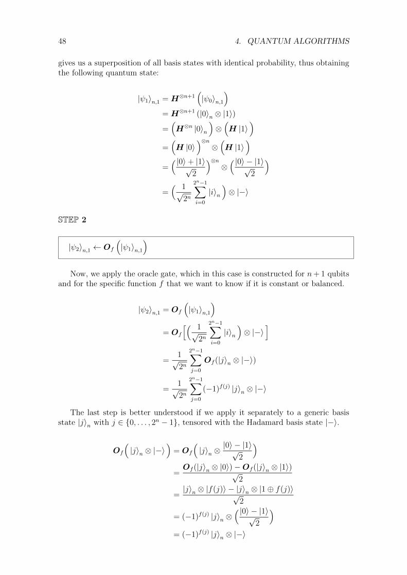
48 4. QUANTUM ALGORITHMS
gives us a superposition of all basis states with identical probability, thus obtainingthe following quantum state:
|ψ1〉n,1 = H⊗n+1(|ψ0〉n,1
)= H⊗n+1 (|0〉n ⊗ |1〉)
=(H⊗n |0〉n
)⊗(H |1〉
)=(H |0〉
)⊗n⊗(H |1〉
)=( |0〉+ |1〉√
2
)⊗n⊗( |0〉 − |1〉√
2
)=( 1√
2n
2n−1∑i=0
|i〉n)⊗ |−〉
STEP 2
|ψ2〉n,1 ← Of
(|ψ1〉n,1
)Now, we apply the oracle gate, which in this case is constructed for n+ 1 qubits
and for the specific function f that we want to know if it is constant or balanced.
|ψ2〉n,1 = Of
(|ψ1〉n,1
)= Of
[( 1√2n
2n−1∑i=0
|i〉n)⊗ |−〉
]=
1√2n
2n−1∑j=0
Of (|j〉n ⊗ |−〉)
=1√2n
2n−1∑j=0
(−1)f(j) |j〉n ⊗ |−〉
The last step is better understood if we apply it separately to a generic basisstate |j〉n with j ∈ 0, . . . , 2n − 1, tensored with the Hadamard basis state |−〉.
Of
(|j〉n ⊗ |−〉
)= Of
(|j〉n ⊗
|0〉 − |1〉√2
)=Of (|j〉n ⊗ |0〉)−Of (|j〉n ⊗ |1〉)√
2
=|j〉n ⊗ |f(j)〉 − |j〉n ⊗ |1⊕ f(j)〉√
2
= (−1)f(j) |j〉n ⊗( |0〉 − |1〉√
2
)= (−1)f(j) |j〉n ⊗ |−〉
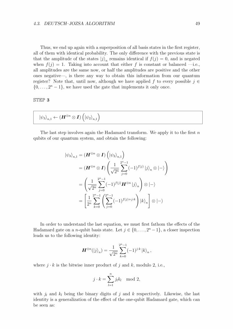
4.3. DEUTSCH–JOZSA ALGORITHM 49
Thus, we end up again with a superposition of all basis states in the first register,all of them with identical probability. The only difference with the previous state isthat the amplitude of the states |j〉n remains identical if f(j) = 0, and is negatedwhen f(j) = 1. Taking into account that either f is constant or balanced —i.e.,all amplitudes are the same now, or half the amplitudes are positive and the otherones negative—, is there any way to obtain this information from our quantumregister? Note that, until now, although we have applied f to every possible j ∈0, . . . , 2n − 1, we have used the gate that implements it only once.
STEP 3
|ψ3〉n,1 ← (H⊗n ⊗ I)(|ψ2〉n,1
)The last step involves again the Hadamard transform. We apply it to the first n
qubits of our quantum system, and obtain the following:
|ψ3〉n,1 = (H⊗n ⊗ I)(|ψ2〉n,1
)= (H⊗n ⊗ I)
(1√2n
2n−1∑j=0
(−1)f(j) |j〉n ⊗ |−〉
)
=
(1√2n
2n−1∑j=0
(−1)f(j)H⊗n |j〉n
)⊗ |−〉
=
[1
2n
2n−1∑k=0
(2n−1∑j=0
(−1)f(j)+j·k
)|k〉n
]⊗ |−〉
In order to understand the last equation, we must first fathom the effects of theHadamard gate on a n-qubit basis state. Let j ∈ 0, . . . , 2n− 1, a closer inspectionleads us to the following identity:
H⊗n(|j〉n) =1√2n
2n−1∑k=0
(−1)j·k |k〉n ,
where j · k is the bitwise inner product of j and k, modulo 2, i.e.,
j · k =n∑l=1
jlkl mod 2,
with jl and kl being the binary digits of j and k respectively. Likewise, the lastidentity is a generalization of the effect of the one-qubit Hadamard gate, which canbe seen as:

50 4. QUANTUM ALGORITHMS
H(|j〉) =1√2
(|0〉+ (−1)j |1〉
)=
1√2
1∑k=0
(−1)jk |k〉
STEP 4
k ← measure the first register of |ψ3〉n,1
Finally, we are able to measure the qubits, thus destroying the information insidethe register and obtaining a number k ∈ 0, . . . , 2n−1 according to the probabilitydistribution given by the amplitudes
αk =2n−1∑j=0
(−1)f(j)+j·k.
Let us have a closer look to the probability of obtaining k = 0. As explainedin Chapter 3, in accordance with the laws of quantum mechanics the probabilityof obtaining a certain basis state |k〉n is equal to the square of the modulus of itsamplitude αk. In this case:
|α0|2 =
∣∣∣∣∣ 1√2n
2n−1∑j=0
(−1)f(j)
∣∣∣∣∣2
It is easy to see that |α0|2 = 1 if and only if the function f is constant for allj ∈ 0, . . . , 2n−1, and that |α0|2 = 0 if and only if the function f is balanced (recallthat we are promised that f is of one of those two natures). Having said that, if wemeasure now the first register and obtain some k, we can conclude that f is constantif k = 0, and that f is balanced otherwise. With just a single evaluation of f wehave answered the question, as opposed to the 2n−1 + 1 evaluations needed in theclassical version. A circuit representation of Deutsch-Jozsa algorithm is displayedin Figure 4.2.
The previous algorithm has much more profound implications than the posibil-ity of solving Deutsch’s problem exponentially faster with the help of a quantum
Figure 4.2: Circuit representation of Deutsch-Jozsa algorithm
|0〉n H⊗n
Of
H⊗n k
|1〉 H
|ψ0〉 |ψ1〉 |ψ2〉 |ψ3〉 |ψ4〉

4.4. SIMON’S ALGORITHM 51
computer. It also tells us that, relative to an oracle —i.e., a black box that solves acertain problem or function, namely f— we can establish a difference between theclasses P and EQP. Note that this does not imply that P 6= EQP, it just tells usthat there exists an oracle separation between P and EQP.
4.4 Simon’s Algorithm
4.4.1 Definition
Let f : 0, 1n → 0, 1n be a function such that, for some s ∈ 0, 1n withs 6= (0, 0, . . . , 0), f(j) = f(k) if and only if either j = k or j ⊕ k = s for allj, k ∈ 0, 1n —where ⊕ is again the bitwise exclusive disjunction operation, alsocalled bitwise xor—. Simon’s problem is defined as: given such an f as a blackbox, figure out the value of s, which is usually called the xor-mask of f . Both theproblem and the quantum algorithm we proceed to explain were both first presentedin [106] by Daniel R. Simon, hence their names.
Simon’s problem can also be seen as an instance of the hidden subgroup problem,where G = (0, 1n,⊕), X ⊆ 0, 1n is any finite set, and K = 0, s for somes ∈ 0, 1n. In the classical version, a solution for this problem requires that wefind a pair of values x, y ∈ 0, 1n such that f(x) = f(y), and then compute x⊕ y.This solution requires O(2n/2) evaluations of f in the worst case whereas, as will beproved later, Simon’s algorithm only needs O(n) evaluations of f .
SETUP
|ψ0〉n,n ← |0〉n ⊗ |0〉n
In this algorithm, we need 2n qubits, all of them initialized at |0〉.
STEP 1
|ψ1〉n,n ← (H⊗n ⊗ I⊗n)(|ψ0〉n,n
)We first apply the Hadamard transformation to the first half of our qubit set,
thus obtaining the following quantum state.
|ψ1〉n,n = (H⊗n ⊗ I⊗n)(|ψ0〉n,n
)= (H⊗n ⊗ I⊗n)(|0〉n ⊗ |0〉n)
= (H⊗n |0〉n)⊗ (|0〉n)
=1√2n
2n−1∑j=0
|j〉n ⊗ |0〉n

52 4. QUANTUM ALGORITHMS
STEP 2
|ψ2〉n,n ← Of
(|ψ1〉n,n
)Next, we use the oracle gate, built particularly for the function f . Note that,
thanks to quantum paralelism, we apply here the function f to all possible valuesin 0, 1n with just a single iteration of Of . Thus, all possible values of f are nowpresent in the second register.
|ψ2〉n,n = Of
(|ψ1〉n,n
)= Of
(1√2n
2n−1∑j=0
|j〉n ⊗ |0〉n
)
=1√2n
2n−1∑j=0
Of (|j〉n ⊗ |0〉n)
=1√2n
2n−1∑j=0
|j〉n ⊗ |f(j)〉n
STEP 3
δ ← measure the second register of |ψ2〉n,n
|ψ3〉n ← |ψ2〉n,n after measuring the second register
In this step we see for the first time the true effects of measuring part of ourquantum system before completing the execution of an algorithm. If we measure nowthe second register, we shall end up with a value δ = f(j) for a certain j ∈ 0, 1n.Thus, only the values in f−1(δ) will remain in the first register —before measuring,they were the only ones tensored with |δ〉—. In any case, as f−1(δ) = j, j ⊕ s—we remark that j⊕ k = s if and only if j⊕ s = k—, we end up with the followingquantum state:
|ψ3〉n =1√2
(|j〉n + |j ⊕ s〉n
)STEP 4
|ψ4〉n ←H⊗n (|ψ3〉n)
The last transformation we apply to our quantum system is, again, the Hadamardgate.1 Before that, we could have measured the first register and obtain a certain
1Did we mention that it is one of the important ones?

4.4. SIMON’S ALGORITHM 53
value in f−1(δ) = j, j ⊕ s. However, in that case we would have ended with thesame information as if we had just made a single classical evaluation of f . TheHadamard gate, on the other hand, will let us obtain much more information thanfrom a single evaluation of f : it will give us some precious information about s.Following a similar reasoning as with Deutsch-Jozsa algorithm, we end up with:
|ψ4〉n = H⊗n (|ψ3〉n)
= H⊗n[
1√2
(|j〉n + |j ⊕ s〉n
)]=
1√2
(H⊗n |j〉n +H⊗n |j ⊕ s〉n
)=
1√2
[1√2n
2n−1∑k=0
(−1)j·k |k〉n +1√2n
2n−1∑k=0
(−1)(j⊕s)·k |k〉n
]
=1√2n+1
2n−1∑k=0
(−1)j·k+(j⊕s)·k |k〉n
=1√2n+1
2n−1∑k=0
(−1)j·k[1 + (−1)s·k
]|k〉n
STEP 5
ω ← measure |ψ4〉n
Let us suppose that we measure our quantum system right now. It is clear thatthe current amplitudes of the basis states are
αk =
∣∣∣∣ 1√2n+1
[1 + (−1)s·k
]∣∣∣∣2for k ∈ 0, 1n.
However, it can be noted that αk 6= 0 if and only if s · k ≡ 0 mod 2, whichhappens for half the values of k necessarily. Even more, in those cases the amplitudeis equal to 1/2n−1. Analyzing the outcome, we have ended up with some ω suchthat ω · s ≡ 0 mod 2. If we are able to find n − 1 linearly independent values ofω, namely ω1, . . . , ωn−1, we will arrive at a system of equations whose solutions are0 and s. Before proving this, let us explain the performance of Simon’s algorithmwith a worked-out example.
4.4.2 Example with n = 4
Let us suppose that we are given as a black box a function that fulfills therequirements of Simon’s problem. This function, namely f : 0, 14 → 0, 14, hasthe following outcome:

54 4. QUANTUM ALGORITHMS
Figure 4.3: Circuit representation of Simon’s algorithm (one iteration)
|0〉n H⊗n
Of
H⊗n ω
|0〉n δ
|ψ0〉 |ψ1〉 |ψ2〉 |ψ3〉 |ψ4〉 |ψ5〉
f(0) = f(5) = 0f(1) = f(4) = 1f(2) = f(7) = 2f(3) = f(6) = 3f(8) = f(13) = 4f(9) = f(12) = 5f(10) = f(15) = 6f(11) = f(14) = 7
Of course, as the function is given as a black box, this information is only avail-able to us if we evaluate f(j) for all j ∈ 0, . . . , 15. A closer inspection of thesevalues tells us that this function has in fact a xor-mask and that its value is s = 5.Our objective is to arrive at this knowledge without evaluating f classically for allvalues in 0, 14.
Now, let us suppose that we do not know this information yet. As a start,Simon’s algorithm would need the quantum state
|ψ0〉4,4 = |0〉4 ⊗ |0〉4 .
After applying the Hadamard gate, we would obtain
|ψ1〉4,4 =1
16
15∑j=0
|j〉4 ⊗ |0〉4
and, after the oracle gate, our system is in the state
|ψ2〉4,4 =1
16
15∑j=0
|j〉4 ⊗ |f(j)〉4 .
If we make use of the information we know (but we should not!) about f , wecould see the previous equation as:
|ψ2〉4,4 =1
8
[(|0〉4 + |5〉4
)⊗ |0〉4 +
(|1〉4 + |4〉4
)⊗ |1〉4 +
(|2〉4 + |7〉4
)⊗ |2〉4 +(
|3〉4 + |6〉4)⊗ |3〉4 +
(|8〉4 + |13〉4
)⊗ |4〉4 +
(|9〉4 + |12〉4
)⊗ |5〉4 +(
|10〉4 + |15〉4)⊗ |6〉4 +
(|11〉4 + |14〉4
)⊗ |7〉4
]

4.4. SIMON’S ALGORITHM 55
Please note again that the previous state is actually happening inside our quan-tum computer whether or not we know the values for f(j). As we have constructedour oracle gate using f as a black box, it necessarily has the previous effect on theHadamard state.
Up until now all steps were deterministic. However, the next step, the measure-ment of the second register, will have a non-deterministic outcome. Let us supposethat we measure it and obtain, for example, the value δ = 6. Necessarily, ourquantum system is now in the state
|ψ3〉4 =1√2
(|10〉4 + |15〉4)
and, if we apply now the Hadamard transform, we end up with
|ψ4〉4 =1√25
15∑k=0
(−1)j·k[1 + (−1)s·k
]|k〉n ,
where j ∈ f−1(6) = 10, 15 and s is the (yet unknown!) xor-mask of f .
As can be seen, the values we get of j and δ are unimportant. What we needis the outcome of the measurement of our quantum system at this moment. Aspreviously said, we will end up with a number ω such that s · ω = 0 mod 2. In thiscase, ω ∈ 0, 2, 5, 7, 8, 10, 13 for s = 5, where all of them have the same probabilityof coming up.
Let us suppose that we have run three complete iterations of Simon’s algorithm,and obtain ω1 = 2, ω2 = 7 and ω3 = 10. Thus, draining from the fact that ωi · s = 0mod 2 for all of them, if we define s = s3s2s1s0 as the bitwise representation of s(with si ∈ 0, 1), we can consider the system of equations
s1 = 0 mod 2s2 + s1 + s0 = 0 mod 2
s3 + s2 + s0 = 0 mod 2,
with each one of the equations giving us respectively the following set of solutions:
Ω1 = 0, 1, 4, 5, 8, 9, 12, 13,Ω2 = 0, 3, 5, 6, 8, 11, 13, 14,Ω3 = 0, 1, 4, 5, 10, 11, 14, 15.
Clearly, as our xor-mask s must satisfy all previous equations, we can deducethat s ∈ Ω1 ∩ Ω2 ∩ Ω3 = 0, 5 and, as s 6= 0 by definition, we can conclude thatour xor-mask is, in fact, s = 5. Note that as the process of obtaining the differentvalues for ω is non-deterministic, the remaining question is this: how many times dowe have to execute Simon’s algorithm in order to obtain such a system with enoughprobability?

56 4. QUANTUM ALGORITHMS
4.4.3 Proof of correctness
Theorem 4.4.1. Simon’s algorithm finds the correct solution for Simon’s problemin O(n) steps with probability greater than 1/3.
Proof. Let us suppose that we have obtained m linearly independent equations,namely with ω1, . . . , ωm. Then, the probability of obtaining another linearly inde-pendent equation in the next interation of Simon’s algorithm is
2n − 2m
2n.
Thus, assuming n ≥ 3, the probability of obtaining n − 1 linearly independentequations after n− 1 iterations of Simon’s algorithm is
P =
(1− 1
2n
)(1− 2
2n
)· · ·(
1− 2n−2
2n
)≥
(1−
n∑k=2
1
2k
)≥ 2n−1 − 1
2n>
1
3
Even though Simon’s algorithm is of little practical use in precisely the sameway as Deutsch’s and Deutsch-Jozsa’s are, it shows once more that there exist prob-lems such that a quantum computer is capable of solving them efficiently while aclassical one is not. In fact, Simon’s algorithm shows that there exist problems suchthat a quantum Turing machine is exponentially faster than a probabilistic Turingmachine [91]. The difference between Simon’s and Deutsch-Jozsa is that the lattercan be solved by a PTM with an arbitrarily small error, while the former wouldtake an exponential time to solve with such a machine. Finally, although Simon’salgorithm stablishes an oracle separation between BPP and BQP, we still do notknow if BPP 6= BQP, as Simon’s problem depends on a black box. An adiabaticversion of Simon’s algorithm can be found in [66].
4.5 Shor’s Factoring Algorithm
4.5.1 Introduction
Let us begin with a problem in number theory that stems from one of the mostwell known theorems of all time:
Definition 4.5.1. Let N ∈ Z≥0, the fundamental theorem of arithmetic tells us thatthere exists a unique factorization of N as a product of prime powers:
N = pα11 p
α22 · · · p
αkk =
k∏i=1
pαii .
The prime factorization problem, or PFP, is the problem of finding such a factor-ization for a given number N ∈ Z≥0.
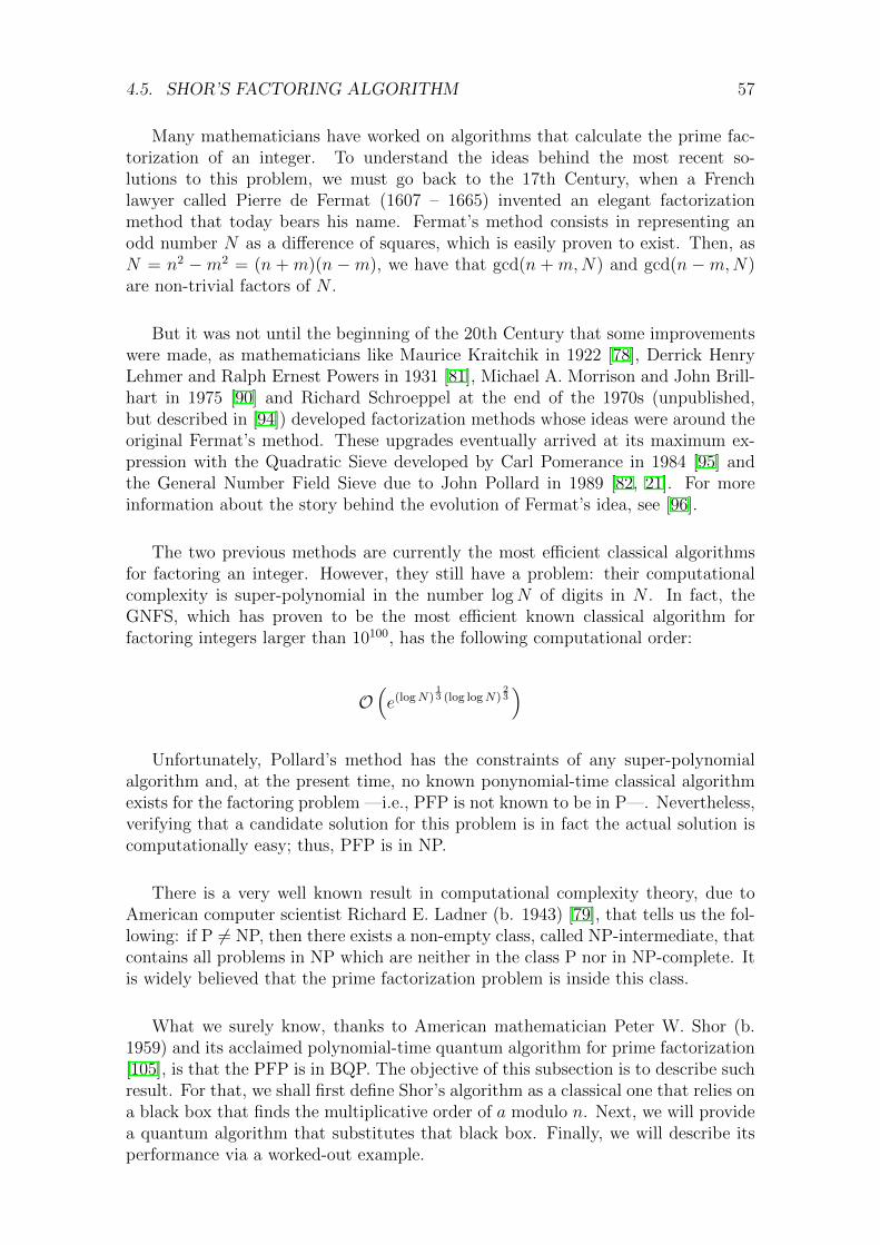
4.5. SHOR’S FACTORING ALGORITHM 57
Many mathematicians have worked on algorithms that calculate the prime fac-torization of an integer. To understand the ideas behind the most recent so-lutions to this problem, we must go back to the 17th Century, when a Frenchlawyer called Pierre de Fermat (1607 – 1665) invented an elegant factorizationmethod that today bears his name. Fermat’s method consists in representing anodd number N as a difference of squares, which is easily proven to exist. Then, asN = n2 −m2 = (n + m)(n −m), we have that gcd(n + m,N) and gcd(n −m,N)are non-trivial factors of N .
But it was not until the beginning of the 20th Century that some improvementswere made, as mathematicians like Maurice Kraitchik in 1922 [78], Derrick HenryLehmer and Ralph Ernest Powers in 1931 [81], Michael A. Morrison and John Brill-hart in 1975 [90] and Richard Schroeppel at the end of the 1970s (unpublished,but described in [94]) developed factorization methods whose ideas were around theoriginal Fermat’s method. These upgrades eventually arrived at its maximum ex-pression with the Quadratic Sieve developed by Carl Pomerance in 1984 [95] andthe General Number Field Sieve due to John Pollard in 1989 [82, 21]. For moreinformation about the story behind the evolution of Fermat’s idea, see [96].
The two previous methods are currently the most efficient classical algorithmsfor factoring an integer. However, they still have a problem: their computationalcomplexity is super-polynomial in the number logN of digits in N . In fact, theGNFS, which has proven to be the most efficient known classical algorithm forfactoring integers larger than 10100, has the following computational order:
O(e(logN)
13 (log logN)
23
)Unfortunately, Pollard’s method has the constraints of any super-polynomial
algorithm and, at the present time, no known ponynomial-time classical algorithmexists for the factoring problem —i.e., PFP is not known to be in P—. Nevertheless,verifying that a candidate solution for this problem is in fact the actual solution iscomputationally easy; thus, PFP is in NP.
There is a very well known result in computational complexity theory, due toAmerican computer scientist Richard E. Ladner (b. 1943) [79], that tells us the fol-lowing: if P 6= NP, then there exists a non-empty class, called NP-intermediate, thatcontains all problems in NP which are neither in the class P nor in NP-complete. Itis widely believed that the prime factorization problem is inside this class.
What we surely know, thanks to American mathematician Peter W. Shor (b.1959) and its acclaimed polynomial-time quantum algorithm for prime factorization[105], is that the PFP is in BQP. The objective of this subsection is to describe suchresult. For that, we shall first define Shor’s algorithm as a classical one that relies ona black box that finds the multiplicative order of a modulo n. Next, we will providea quantum algorithm that substitutes that black box. Finally, we will describe itsperformance via a worked-out example.

58 4. QUANTUM ALGORITHMS
4.5.2 Definition: Classical part
Let N ∈ Z≥0, we proceed to define Shor’s algorithm for factoring N .
STEP 1
x← random integer such that 1 < x < Nd← gcd(x,N)
It is clear that, if d > 1, we have already found a factor of N . However, theprobability of such an unlikely event is small, and in this case we proceed to nextstep. Note that the computational complexity of this step —i.e., of calculating thegreatest common divisor of x and N— has order O(log2N) [76].
STEP 2
r ← ON(x)
This is the step that we shall resolve with the aid of a quantum computer, as willbe explained later. For now, let us recall that the multiplicative order of x moduloN , provided that gcd(x,N) = 1, is defined as
ON(x) = minr ∈ Z>0 : xr ≡ 1 mod N.
Calculating the multiplicative order is a hard problem in the general case, and thebest known classical algorithm that solves it has a super-polynomial computationalcomplexity [36].
Right now, we have obtained a certain r such that r = ON(x). However, notany value of r serves our purposes. At the end of this step, we shall check if r is aneven number and, if that holds, we have to also check if xr/2 + 1 6≡ 0 mod N . Ifany of those two conditions fail, we shall go back to the beginning of the algorithm,and repeat it again with a different random value for x. The unavoidable questionis: what is the probability of not making it?
Theorem 4.5.2. Let N ∈ Z≥0 such that 2 - N and whose prime factorization is
N = pα11 p
α22 · · · p
αkk .
Suppose x is chosen at random, with 1 < x < N and gcd(x,N) = 1, and letr = ON(x). Then:
Prob[(2 | r) ∧ (xr/2 + 1 6≡ 0 mod N)
]≥ 1− 1
2k−1
Proof. [48] Appendix B.
In other words, the probability of obtaining a number x that fulfills all theconditions of the algorithm is greater than 1/2 in the worst case (i.e., when N hasonly two different prime factors).
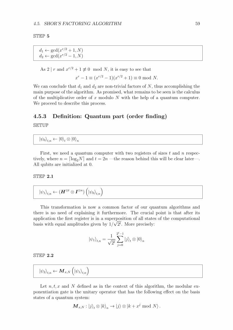
4.5. SHOR’S FACTORING ALGORITHM 59
STEP 5
d1 ← gcd(xr/2 + 1, N)d2 ← gcd(xr/2 − 1, N)
As 2 | r and xr/2 + 1 6≡ 0 mod N , it is easy to see that
xr − 1 ≡ (xr/2 − 1)(xr/2 + 1) ≡ 0 mod N.
We can conclude that d1 and d2 are non-trivial factors of N , thus accomplishing themain purpose of the algorithm. As promised, what remains to be seen is the calculusof the multiplicative order of x modulo N with the help of a quantum computer.We proceed to describe this process.
4.5.3 Definition: Quantum part (order finding)
SETUP
|ψ0〉t,n ← |0〉t ⊗ |0〉n
First, we need a quantum computer with two registers of sizes t and n respec-tively, where n = dlog2Ne and t = 2n —the reason behind this will be clear later—.All qubits are initialized at 0.
STEP 2.1
|ψ1〉t,n ← (H⊗t ⊗ I⊗n)(|ψ0〉t,n
)This transformation is now a common factor of our quantum algorithms and
there is no need of explaining it furthermore. The crucial point is that after itsapplication the first register is in a superposition of all states of the computationalbasis with equal amplitudes given by 1/
√2t. More precisely:
|ψ1〉t,n =1√2t
2t−1∑j=0
|j〉t ⊗ |0〉n
STEP 2.2
|ψ2〉t,n ←Mx,N
(|ψ1〉t,n
)Let n, t, x and N defined as in the context of this algorithm, the modular ex-
ponentiation gate is the unitary operator that has the following effect on the basisstates of a quantum system:
Mx,N : |j〉t ⊗ |k〉n → |j〉 ⊗ |k + xj mod N〉 .

60 4. QUANTUM ALGORITHMS
This transformation is unitary, and its construction takes O(log3N) steps [105].Thus, as will be clear at the end of this subsection, it represents the bottleneck ofShor’s algorithm.
|ψ2〉t,n = Mx,N
(|ψ1〉t,n
)=
1√2t
2t−1∑j=0
Mx,N (|j〉t ⊗ |0〉n)
=1√2t
2t−1∑j=0
|j〉t ⊗∣∣xj mod N
⟩n
Thanks again to quantum parallelism, we have now generated all powers of xmodulo N simultaneously. From now on, in order to make the tracking of thealgorithm cleaner, we shall suppose that r is a power of 2. In this case, our currentquantum state can be expressed as follows:
|ψ2〉t,n =1√2t
r−1∑b=0
2t
r−1∑
a=0
|ar + b〉t
⊗ |xb mod N〉n
The general case where r may not be a power of 2 is more difficult to express,
and is better to explain it in the part devoted to the example.
STEP 2.3
δ ← measure the second register
|ψ3〉t ← |ψ2〉t,n after measuring the second register
Let us suppose that, for a certain b0 ∈ 0, . . . , r−1, we obtain the value δ = xb0
mod N . Thus, the computer is now in the following quantum state:
|ψ3〉t =
√r
2t
2t
r−1∑
a=0
|ar + b0〉t .
Note that now we only have 2t/r terms in the sum, instead of the previous 2t ones,and that the value we are looking for (i.e., r) is beginning to surface inside ourquantum system in the form of a period. The next step will provide us with a toolcapable of extracting this period from a quantum state.
STEP 2.4
|ψ4〉t ← F n (|ψ3〉t)

4.5. SHOR’S FACTORING ALGORITHM 61
This step requires that we define a new quantum gate: the quantum discreteFourier transform, or QFT, whose effect on the quantum basis states is:
F n : |j〉n →1√2n
2n−1∑k=0
e−2πijk/2n |k〉n
After applying the QFT to the first register, we can express the obtained stateas follows:
|ψ4〉t = F t (|ψ3〉t)
=
√r
2t
2t
r−1∑
a=0
F t(|ar + b0〉t)
=
√r
2t
2t
r−1∑
a=0
(1√2t
2t−1∑j=0
e−2πij(ar+b0)/2t | j〉t
)
=1√r
2t−1∑j=0
r2t
2t
r−1∑
a=0
e−2πija
2t/r
e−2πijb0/2t | j〉t
=
1√r
(r−1∑k=0
e−2πi krb0
∣∣∣∣k2t
r
⟩t
)Please note that, in order to arrive at the last version of the state, we have
just rearranged the summation order while also using the following property of theexponential sums:
1
N
N−1∑j=0
e2πijk/N =
1 if N | k0 otherwise,
then we can rewrite the state as:
|ψ4〉 =1√r
(r−1∑k=0
e−2πi krb0
∣∣∣∣k2t
r
⟩t
)|xb0〉n
Now, at last, it is time to measure the first register.
STEP 2.5
ω ← measure |ψ4〉t
We obtain, for some unknown k0 ∈ 0, . . . , r − 1 (the probability of obtainingeach of them is the same, but this changes in the general case where r may not bea power of 2):
ω =k02t
rIf ω = 0, we obtain no information and we must come back to the beginning.
If, otherwise, ω 6= 0, we can obtain some information about r (or the actual value

62 4. QUANTUM ALGORITHMS
of r indeed), just by putting ω/2t as a fraction in lowest terms and taking thedenominator. If we call c that denominator and xc 6≡ 1 mod N , then c is a factorof r. If, on the other hand xc ≡ 1 mod N , then r = c and we have obtainedthe multiplicative order of x modulo N . In the former case, we should rerun thequantum part of Shor’s algorithm with xc instead of with x, and by repeating thisprocess a finite number of times we shall end up with the correct value of r. Nowlet us show with an example how Shor’s Algorithm works for a particular input.
4.5.4 Example: Factoring 217
We want to find the prime factors of 217 using Shor’s Factoring Algorithm. First,the algorithm chooses a random integer x such that 1 < x < 217. Let us supposethat we obtain x = 5, which fulfills the first condition: gcd(5, 217) = 1. Now is thetime of finding the multiplicative order of 5 modulo 217, which is achieved with thehelp of a quantum computer.
We calculate t and n and initialize the quantum system. In this case, n =dlog2 217e = 8 and consequently t = 2n = 16. Thus, our quantum registers have thefollowing initial states:
|ψ0〉16,8 ← |0〉16 ⊗ |0〉8
Next, we apply the Hadamard transformation, hence obtaining a superpositionof all basis states in the first register, all with identical amplitudes. This way, allintegers between 0 and 216 − 1 are now somewhere in the first register.
|ψ1〉16,8 ← (H⊗16 ⊗ I⊗8)(|ψ0〉16,8
)
|ψ1〉16,8 =1√216
216−1∑j=0
|j〉16 ⊗ |0〉8
Afterwards, we apply the quantum gate that calculates the powers of 5 modulo217, which has the following effect.
|ψ2〉16,8 ←M 5,217
(|ψ1〉16,8
)
|ψ2〉16,8 = M 5,217
(|ψ1〉16,8
)=
1√216
216−1∑j=0
M 5,217 (|j〉16 ⊗ |0〉8)
=1√216
216−1∑j=0
|j〉16 ⊗∣∣5j mod 217
⟩8

4.5. SHOR’S FACTORING ALGORITHM 63
If we expand the sum, we can alternatively express the result as follows (pleasenote that, for the sake of simplicity, we have omitted the subindices and the tensorproduct operators):
|ψ2〉 =1√216
(|0〉 |1〉+ |1〉 |5〉+ |2〉 |25〉+ |3〉 |125〉+ |4〉 |191〉+ |5〉 |87〉+
|6〉 |1〉+ |7〉 |5〉+ |8〉 |25〉+ |9〉 |125〉+ |10〉 |191〉+ |11〉 |87〉+|12〉 |1〉+ |13〉 |5〉+ |14〉 |25〉+ |15〉 |125〉+ |16〉 |191〉+ |17〉 |87〉+|18〉 |1〉+ |19〉 |5〉+ |20〉 |25〉+ |21〉 |125〉+ |22〉 |191〉+ |23〉 |87〉+|24〉 |1〉+ |25〉 |5〉+ |26〉 |25〉+ |27〉 |125〉+ |28〉 |191〉+ |29〉 |87〉+|30〉 |1〉+ ...)
After a close inspection, we can observe that the values on the second registerare periodic. If we make common factor, we end up with the state:
|ψ2〉 =1√216
((|0〉+ |6〉+ |12〉+ |18〉+...+ |65526〉+ |65532〉) |1〉+
(|1〉+ |7〉+ |13〉+ |19〉+...+ |65527〉+ |65533〉) |5〉+(|2〉+ |8〉+ |14〉+ |20〉+...+ |65528〉+ |65534〉) |25〉+(|3〉+ |9〉+ |15〉+ |21〉+...+ |65529〉+ |65535〉) |125〉+(|4〉+ |10〉+ |16〉+ |22〉+...+ |65530〉) |191〉+(|5〉+ |11〉+ |17〉+ |23〉+...+ |65531〉) |87〉
)Thanks to this representation, it is easier to understand what will happen if we
measure the second register.
δ ← measure the second register
|ψ3〉16 ← |ψ2〉16,8 after measuring the second register
It is clear that we shall obtain a value δ such that δ = 5 j mod 217 for a certainj ∈ 0, . . . , 216 − 1. Thus, δ ∈ 1, 5, 25, 125, 191, 87 (which are the powers of 5modulo 217). Let us suppose that we get δ = 25. The register will collapse into|25〉 and all other possible values will be destroyed and gone forever, the informationabout the rest of possible powers of 5 modulo 217 lost. However, the first registerwill also collapse into the values that were tensored with |25〉, thus discarding theremaining ones. What interests us is that all the basis states tensored with |25〉correspond with the exponents j such that δ = 5j mod 217. More specifically:
|ψ3〉16 =1√
10923(|2〉16 + |8〉16 + |14〉16 + |20〉16 + ...+ |65528〉16 + |65534〉16)
=1√
10923
(10922∑a=0
|6a+ 2〉16
)A pattern has arisen, as the basis states on the first register display some peri-
odic behavior. This period naturally corresponds with the multiplicative order of5 modulo 217, which happens to be equal to 6. Of course, this information is yet

64 4. QUANTUM ALGORITHMS
hidden to us, we are just using some knowledge of the problem for providing a math-ematical explanation of the performance of the algorithm in this particular case. Onthe other hand, the constant 10923 is just a normalization of the amplitudes afterthe collapse of the register, corresponding to the total number of exponents thatreturn 25 modulo 217 between 0 and 216 − 1.
As explained previously, if we want to obtain the period from within the bowelsof our quantum system, we should use the quantum Fourier transform:
|ψ4〉16 ← F 16 (|ψ3〉16)
|ψ4〉16 = F 16 (|ψ3〉16)
= F 16
(1√
10923
10922∑a=0
|6a+ 2〉16
)
=1√
10923
10922∑a=0
F 16
(|6a+ 2〉16
)=
1√10923
10922∑a=0
(1√216
216−1∑k=0
e−2πi(6a+2)k
216 |k〉16
)
=1√216
216−1∑k=0
([1√
10923
10922∑a=0
e−2πi 6ak216
]e−2πi 2k
216 |k〉16
)
Thus, we end up again with a distribution of the amplitudes defined by
αk =1√
216 · 10923
(10922∑a=0
e−2πi 6ak216
)e−2πi 2k
216 ,
which gives us the following probability distribution:
|αk|2 =1
216 · 10923
∣∣∣∣∣10922∑a=0
e−2πi 6ja216
∣∣∣∣∣2
with k = 0, . . . , 216 − 1. If we represent this distribution in a graph, it is easier tounderstand the final steps of the algorithm.

4.5. SHOR’S FACTORING ALGORITHM 65
0 10 000 20 000 30 000 40 000 50 000 60 000 70 0000.0000
0.0002
0.0004
0.0006
0.0008
0.0010
ω ← measure |ψ4〉16)
We then measure the first register, and obtain non-deterministically a value fromone of the seven peaks. The first peak yields a 0, thus forcing us to start again thequantum part of the algorithm. If, otherwise, we obtain a value from the other sixpeaks, we can retrieve (using continued fractions) the order r or a factor of r from it.
Let us explain this last step more formally (we took details for this from [84]).We recall that a continued fraction is represented as
[a0; a1, . . . , aK ] = a0 +1
a1 +1
a2 +1
a3 +1
· · ·+1
aK
where a0 ∈ Z≥0 and a1, . . . , aK ∈ Z>0. Let [a0; a1, . . . , aK ], then there exists aunique q ∈ Q>0 such that q = [a0; a1, . . . , aK ]. We define the k-th convergent of[a0; a1, . . . , aK ], where 0 ≤ k < K, as
qk = [a0; a1 . . . , ak].
Provided a certain q ∈ Q>0, we can compute the members of its correspondingcontinued fraction as follows:

66 4. QUANTUM ALGORITHMS
a0 ← bqcq0 ← q − a0
ak+1 ← b1/qkcqk+1 ← 1/qk − ak+1
Even more, each of the convergents qk can be expressed as qk = bk/ck, wheregcd(bk, ck) = 1 and
b0 ← a0
c0 ← 1
b1 ← a0a1 + 1
c1 ← a1
bk+2 ← ak+2bk+1 + bk
ck+2 ← ak+2ck+1 + ck
It can be proven [84] that we can obtain the period r (or a non trivial factor ofit) from w with the following algorithm: starting at k = 1, we compute bk and ck aspreviously explained from the continued fraction of q = w/2n. Then, we check if
xck ≡ 1 mod N.
If the answer is affirmative, we have obtained the order r or a factor of it; if not, wedo it again for k + 1.
For example, a possible value from the second peak is 10915, and if we divide itby 216 we obtain the continued fraction
10915
65536= [0; 6, 237, 3, 1, 1, 6],
whose first convergent is 16. Thus, as 56 ≡ 1 mod 217 we have that the order (or a
factor of it) is 6.
Another possible example is 32763, a value from the middle peak. Doing thesame operation:
32763
65536= [0; 2, 3276, 3, 3]
from where we obtain a first convergent of 12. In both cases, we have to verify if 6
and 2 are, respectively, the order of 5. The first case returns a positive answer, butthe second forces us to restart the algorithm to get the order of 52. In any case,after a finite number of iterations we finally obtain r = 6.
Remains to be seen if x = 5 and r = 6 fulfill the final conditions of the algorithm.As 6 is an even number, and 56/2 + 1 = 126 6= 0 mod 217, we can finally proceed tothe last step. As explained, we can calculate now two non-trivial factors of 217:
d1 = gcd(126, 217) = 7

4.6. GROVER’S SEARCH ALGORITHM 67
and
d2 = gcd(124, 217) = 31,
which in fact are the only prime factors of 217. Thus ends Shor’s algorithm for thisparticular case.
217 = 7× 31
The first experimental demonstration of Shor’s factoring algorithm came in 2001,[113] when a group at IBM factored 15 into 3 and 5 using a nuclear magneticresonance (NMR) quantum computer with seven spin-1/2 nuclei in a molecule asqubits. In 2007, Shor’s algorithm was implemented with photonic qubits by twodifferent groups [80, 85], with both of them observing quantum entanglement in theprocess. In 2012, number 143 was factored with the help of an adiabatic quantumcomputer [114].
4.6 Grover’s Search Algorithm
4.6.1 Definition
Grover’s search algorithm was first described by Indian-American computer sci-entist Lov K. Grover (b. 1961) in [63, 64, 65], hence its name. The original aimof Grover’s algorithm is the following: we have an unstructured and disorganizeddatabase with 2n elements, identified from now on with the indices 0, . . . , 2n − 1,and we want to find one that satisfies a certain property. The algorithm leans ontwo hypotheses: first, that such an element exists inside the database; and second,that this element is unique.
If we are to search for this mentioned element with a classical computer, in theworst case we will have to check all members of the database, which tells us thatthis problem has a classical computational complexity of O(2n). As will be shown,Grover’s quantum search algorithm will make only O(
√2n) queries to the database,
thus strictly improving the performance of its classical counterpart.
SETUP
|ψ0〉n,1 ← |0〉n ⊗ |1〉
We need a quantum computer with n+ 1 qubits, where the first n qubits will beinitialized at |0〉 and the remaining one at |1〉.
STEP 1
|ψ1〉n,1 ←H⊗n+1(|ψ0〉n,1
)
68 4. QUANTUM ALGORITHMS
In the first proper step of the algorithm, we apply the Hadamard quantum gateto all the qubits in our system. This way, the obtained result is a combination of allbasis states inside our first n qubits, and the |−〉 state in the remaining one.
|ψ1〉n,1 = H⊗n+1(|ψ0〉n,1
)= H⊗n+1 (|0〉n ⊗ |1〉)
=(H⊗n |0〉n
)⊗(H |1〉
)=(H |0〉
)⊗n⊗(H |1〉
)=( |0〉+ |1〉√
2
)⊗n⊗( |0〉 − |1〉√
2
)=( 1√
2n
2n−1∑j=0
|j〉n)⊗ |−〉
For the sake of simplicity, we reintroduce a useful quantum state that will appearmany times throughout the rest of the algorithm. It will also be needed in order todefine one of the key quantum gates of Grover’s Search method, as will be shown inthe next step.
|γ〉n =1√2n
2n−1∑j=0
|j〉n
This definition helps us to express our quantum state as follows:
|ψ1〉n,1 = |γ〉n ⊗ |−〉
STEP 2.1
|ψ2〉n,1 ← Of
(|ψ1〉n,1
)The next step of the algorithm leans on the following assumption: we can build
a quantum gate, called Of , that makes use of a function capable of recognizingthe element of the database we are searching for. This function f can be definedas follows (note that the desired element is identified by the unknown index j0 ∈0, . . . , 2n − 1).
f(j) =
1 if j = j0
0 otherwise
The Of quantum gate is in fact the oracle gate described in previous algorithms,which has the following effect on the basis states of a n+ 1-qubit system
Of : |j〉n ⊗ |k〉 → |j〉n ⊗ |k ⊕ f(j)〉 .
4.6. GROVER’S SEARCH ALGORITHM 69
We recall from Deutsch-Jozsa algorithm that the oracle gate has the followingeffect on the state |j〉n ⊗ |−〉:
Of
(|j〉n ⊗ |−〉
)= (−1)f(j) |j〉n ⊗ |−〉
It can be seen that, in those cases, Of inverts the sign of the amplitude corre-sponding to the basis state that codifies the searched element in the first n qubits,while keeping intact the rest of the amplitudes.
In order to make the explanation and understanding of the algorithm easier andsimpler, we introduce another n-qubit quantum state,
|ρ〉n =1√
2n − 1
2n−1∑j=0j 6=j0
|j〉n ,
whose relationship with the aforedescribed state |γ〉n is
|γ〉n =
√2n − 1√
2n|ρ〉n +
1√2n|j0〉n .
Please note that |ρ〉 depends on the value of j0, but we shall write |ρ〉 instead of|ρ (j0)〉 for the sake of simplicity. It can be observed that the introduction of |ρ〉nhelps in the separation of the searched elemenet |j0〉 from the rest of the quantumbasis states.
Thus, after applying Of to our quantum system it will look like this:
|ψ2〉n,1 = Of
(|ψ1〉n,1
)= Of
(|γ〉n ⊗ |−〉
)= Of
((√2n − 1√
2n|ρ〉n +
1√2n|j0〉n
)⊗ |−〉
)=(√2n − 1√
2n|ρ〉n −
1√2n|j0〉n
)⊗ |−〉
=(|γ〉n −
2√2n|j0〉n
)⊗ |−〉
The motivation behind the last interpretation of |ψ2〉n,1 will become clear in thenext step.
70 4. QUANTUM ALGORITHMS
STEP 2.2
|ψ3〉n,1 ← (Γ n ⊗ I)(|ψ2〉n,1
)For this step, we must construct a new quantum gate, denoted by Γ n, that
will affect only the first n qubits. The remaining qubit will remain intact —this isrepresented with the single-qubit identity gate I—. The definition of Γ n is:
Γ n = 2 |γ〉n 〈γ|n − I⊗n
Let us see what happens when we apply this new quantum gate to the first nqubits of our quantum state |ψ2〉n,1 defined in the previous step.
Γ n (|ψ2〉n) =(2 |γ〉n 〈γ|n − I
⊗n)(|γ〉n − 2√2n|j0〉n
)= 2 |γ〉n 〈γ|γ〉n −
4√2n|γ〉n 〈γ|j0〉n − |γ〉n +
2√2n|j0〉n
= 2 |γ〉n −4
2n|γ〉n − |γ〉n +
2√2n|j0〉n
=2n−2 − 1
2n−2|γ〉n +
2√2n|j0〉n
For this, we have used the definition of the inner product seen in Section 3.3 tocalculate
〈γ|γ〉n = 1
and
〈γ|i0〉n =1√2n.
The Γ n gate is also called Grover diffusion operator, and can also be seen as
Γ n = (H⊗n)(2 |0〉n 〈0|n − I⊗n)(H⊗n),
which is a much more painless way of implementing it in practice. Steps 2.1 and 2.2are usually treated as a single step, represented by the Grover gate
G = (Γ n ⊗ I)(Of ).
STEP 3
In order to achieve the objective of Grover’s algorithm, one must apply theG gaterepeatedly until the probability of obtaining the index j0 is maximal —a generaloverview of the algorithm can be seen in Figure 4.4—. After the desired probabilityhas been reached, we measure the first n-qubit register, and obtain the index j0.The optimal number of times G is applied has order O(
√2n), which will be proved
later. But first, let us explain the behavior of the algorithm with an example.

4.6. GROVER’S SEARCH ALGORITHM 71
|0〉 /n H⊗nOf
Γ n · · ·
|1〉 H · · ·
Repeat O(√
2n) times
︸ ︷︷ ︸Figure 4.4: Circuit representation of Grover’s Search Algorithm
4.6.2 Example with n = 4 qubits
Let us illustrate how Grover’s Search works with this exemplifying case: supposewe have an unstructured database with its elements listed as 0, 1, . . . , 15 indexed via4 qubits, and that we want to find a certain item that is indexed with the number7 —note that we do not know this yet, but it can be supposed in order to explainthe algorithm straightforwardly—.
As previously explained, we need a quantum computer with n+1 qubits, where nis the number of bits needed for codifying the indices of the members of the database—in this case, n = 4—. In order to correctly setup our quantum system, the first4 qubits must be in the state |0〉 and the remaining one must be in the state |1〉.Thus, our quantum system begins as follows:
|ψ0〉4,1 = |0〉4 ⊗ |1〉
The first transformation we apply to the quantum system is the Hadamard gate,or H , which converts it to the following state:
|ψ1〉4,1 = (H⊗4 |0〉4)⊗ (H |1〉)
=(1
4
15∑j=0
|j〉4)⊗ |−〉
We remind the reader that from now on we will make use of the states |γ〉4 and|ρ〉4 in the interest of simplifying the writing of the whole process.
|γ〉4 =1
4
15∑j=0
|j〉4
|ρ〉4 =1√15
15∑j=0j 6=7
|j〉4
|γ〉4 =
√15
4|ρ〉4 +
1
4|7〉4

72 4. QUANTUM ALGORITHMS
The introduction of these states allows us to write |ψ1〉4,1 as:
|ψ1〉4,1 =
(√15
4|ρ〉4 +
1
4|7〉4
)⊗ |−〉
On STEP 2.1 we make use of the transformation Of , which applies to all possiblestates inside the first 4 qubits an oracle f that identifies 7 as the correct index forthe element we are looking for.
|ψ2〉4,1 = Of (|ψ1〉4,1)
= Of
[(√15
4|ρ〉4 +
1
4|7〉4
)⊗ |−〉
]
=
(√15
4|ρ〉4 −
1
4|7〉4
)⊗ |−〉
=
(|γ〉4 −
1
2|7〉4)⊗ |−〉
On STEP 2.2, we apply the quantum gate Γ 4 to the first 4 qubits of the computer.We use |ρ〉4 to make more clear which part of the state has the index 7 in it andwhich one does not have it.
Γ 4
(|γ〉4 −
1
2|7〉4
)= (2 |γ〉4 〈γ|4 − I)
(|γ〉4 −
1
2|7〉4)
= 2 |γ〉4 〈γ|γ〉4 − |γ〉4 − |γ〉4 〈γ|7〉4 +1
2|7〉4
= 2 |γ〉4 − |γ〉4 −1
4|γ〉4 +
1
2|7〉4
=3
4|γ〉4 +
1
2|7〉4
=3√
15
16|ρ〉4 +
11
16|7〉4
|ψ3〉4,1 =(3√
15
16|ρ〉4 +
11
16|7〉4
)⊗ |−〉
Thus, we have completed the first iteration of G, and if we are to measure ourquantum state now, we have a probability
p =(11
16
)2
=121
256≈ 0.4726
of obtaining the index 7, and a probability
p =(3√
15
16
)2
=135
256≈ 0.5274

4.6. GROVER’S SEARCH ALGORITHM 73
of obtaining any other index. As can be seen, the probability of finding the searchedelement is greater than of finding any other element, but is still not big enough,which tells us that at least another round of the algorithm is needed.
We repeat again the application of G. First, we apply Of and end up with thefollowing quantum state, defined again as a combination of |γ〉4 and |7〉4.
|ψ4〉4,1 = Of,4(|ψ3〉4,1)
=
(3√
15
16|ρ〉4 −
11
16|7〉4
)⊗ |−〉
=
(3
4|γ〉4 −
14
16|7〉4)⊗ |−〉
And then we apply Γ 4.
|ψ5〉4 = (2 |γ〉4 〈γ|4 − I)
(3
4|γ〉4 −
14
16|7〉4)
=3
2|γ〉4 〈γ|γ〉4 −
7
4|γ〉4 〈γ|7〉4 −
3
4|γ〉4 +
7
8|7〉4
=5
16|γ〉4 +
7
8|7〉4
=5√
15
64|ρ〉4 +
61
64|7〉4
Thus, after two iterations of G we end up with a state whose possibility ofreturning the index i0 is
p =(61
64
)2
=3721
4096≈ 0.9084,
which gives us a fairly enough chance of completing the execution of Grover’s SearchAlgorithm successfully. However, how can we be sure that we have obtained the max-imum probability of retrieving the desired element from the database if we cannotmeasure the amplitudes inside our quantum register? Even more, whence comes therequired order of O(
√2n) needed in the number of iterations of G?
Both questions are pivotal in the correct performance of the algorithm. Let usshow their significance with a simple example: what happens if we continue applyingthe G gate to our quantum system?
If we apply G once more, we will have the following two states, the first afterOf and the second after Γ 4.
|ψ6〉 =5
16|γ〉4 −
33
32|7〉4

74 4. QUANTUM ALGORITHMS
|ψ7〉 = −13√
15
256|ρ〉4 −
251
256|7〉4
As can be seen, the probability of obtaining index 7 now is
p =(251
256
)2
≈ 0.9613.
Yet, if we are still not satisfied with a 96% chance of success, we can run over Gonce again, and obtain first
|ψ8〉 = −13
64|γ〉4 −
238
256|7〉4
and finally
|ψ9〉 = −342√
15
2048|ρ〉4 +
1562
2048|7〉4 ,
which gives us a probability
p =(1562
2048
)2
≈ 0.5817
of obtaining |7〉4. Yes, it seems that to unabatedly perform numberless iterations ofG does not guarantee a continuous increment in the probability of success.2 Evenmore, it can waste all previously done work. We shall see why this has happened inthe next section.
4.6.3 Proof of correctness
In this section we sketch a proof of the correctness of Grover’s algorithm. Themain ideas behind this proof are taken from [28], and will come in handy in thenext subsection, where different and more general versions of the database searchalgorithm are discussed.
Theorem 4.6.1. Grover’s Search Algorithm for a unique solution needs m ∼ O(√
2n)iterations of G for maximizing the probability of obtaining the desired element withunknown index j0.
Proof. First, we are interested in redefining all the possible states that occur duringthe execution of the algorithm as a function of the different amplitudes involved.As was shown earlier, the only amplitude that will differ from the rest after ev-ery Grover’s iteration is the one associated with the basis state that identifies thesearched element. Thus, suffices to define the generic state in the following way:
|ψ(α, β)〉n = α |j0〉n + β
2n−1∑j=0j 6=j0
|j〉n .
2“There is thy gold, worse poison to men’s souls.” (Romeo and Juliet, Act 5, Scene 1)

4.6. GROVER’S SEARCH ALGORITHM 75
With amplitudes α and β constrained to
|α|2 + (2n − 1)|β|2 = 1.
Note that we are only having into account the first register, the one with nqubits. The remaining qubit will behave as explained before, starting at |1〉 andremaining as |−〉 throughout the rest of the algorithm, but for the sake of simplicitywill be omitted during the proof.
Let us see what happens when we apply all quantum gates that make up theGrover transform Gn to a generic state |ψ(α, β)〉n. First, we employ Of , whichrecognizes the searched element and flips its amplitude. Thus, after Of we obtain
|ψ′(α, β)〉n = −α |j0〉n + β
2n−1∑j=0j 6=j0
|j〉n
In order to apply the Γn quantum gate, it is interesting to previously see ourcurrent state as a function of |γ〉n, as was done before:
|ψ′(α, β)〉n = −(α + β) |j0〉n +√
2nβ |γ〉n .We are finally in condition of applying Γ n:
|ψ′′(α, β)〉n = Γ n
(|ψ′(α, β)〉n
)= Γ n
(− (α + β) |j0〉n +
√2nβ |γ〉n
)=(
2 |γ〉n 〈γ|n − I⊗n)(− (α + β) |j0〉n +
√2nβ |γ〉n
)= (α + β) |j0〉n +
(2√
2nβ − 2√2n
(α + β)−√
2nβ)|γ〉n
=(2n−1 − 1
2n−1α +
2n − 1
2n−1β)|j0〉n +
(− 1
2n−1α +
2n−1 − 1
2n−1β)|γ〉n
Now that we know the effect Gn makes to a generic state, we are in condition ofpredicting in which iteration of the algorithm we have more possibilities of obtainingthe desired element i0. If we define
|ψk+1(αk+1, βk+1)〉n = Gn(|ψk(αk, βk)〉n)
where
α1 = β1 =1√2n
and
αk+1 =2n−1 − 1
2n−1αk +
2n − 1
2n−1βk
βk+1 = − 1
2n−1αk +
2n−1 − 1
2n−1βk
76 4. QUANTUM ALGORITHMS
for j ≥ 1, then we can try to find a more tractable closed-form formula for theamplitude of i0. Note that, for j = 0, it is not possible to define |ψ0〉 as a functionof α0 and β0, thus only the cases where j ≥ 1 will be defined as such.
If we designate θ such that
sin2 θ =1
2n,
we can easily prove by induction that
αj = sin((2j − 1)θ)
and that
βj =1√
2n − 1cos((2j − 1)θ).
Let us suppose now that, for an unknown step j = m + 1 (note that m isequivalent to the number of times we have applied Gn), we want to assure thatαm = 1. This occurs when
(2m+ 1)θ =π
2,
and expressly, when
m =π − 2θ
4θ.
Obviously, we can not perform a non-integer number of iterations of Gn. If wetake
m =⌊ π
4θ
⌋,
we can conclude that the number of iterations of Gn needed for achieving the max-
imum probability of success is closeπ
4
√2n (note that
θ ≈ sin θ =1√2n
when 2n is large enough). Thus, we can conclude that the number m of iterationsof Gn has order
m ∼ O(√
2n).
4.6.4 Mutiple solutions
The main limitation of Grover’s Search Algorithm deals with the number of so-lutions: it assumes that there is one and only one element in the database thatmatches our search. As will be seen in Chapter 5, there are many cases in whichGrover’s Search may prove useful, but in which the number of solutions is unknown,or maybe we do not even know if there is indeed a solution. In this subsection weproceed to explain an alternate version of Grover’s Algorithm that originally ap-peared in [28] which takes care of this drawback.
Let us suppose that we have an unstructured database, indexed by 0, 1, . . . , 2n−1.We are interested in finding an element inside the database that fulfills a certain

4.6. GROVER’S SEARCH ALGORITHM 77
property, but we do not know if such an element exists, or if there are more thanone. We name A ⊆ 0, 1, . . . , 2n − 1 the set of possible solutions, with |A| = tand t ∈ 0, 1, . . . , 2n − 1. At first sight, one can only hope to just obtain the sameperformance results as in the original Grover’s Algorithm just by applying G thesame number of steps. However, it is easy to find a counterexample showing thatthe probability of success after π
4
√2n iterations changes dramatically when t 6= 1.
In order to show how this variation of the algorithm works, we define B = A,with |B| = 2n− t. Following a similar approach, we can assume that every quantumstate of our system after first applying globally the Hadamard transform can beexpressed as
|ψ(α, β)〉n = α∑i∈A
|i〉n + β∑i∈B
|i〉n ,
wheretα2 + (2n − t)β2 = 1.
We only take into account the first n qubits, as previously done. We would like toclarify that the algorithm is essentially the same, so there is no need for explainingit again. The only substantial change is the expected number of iterations of Gneeded for maximizing the probability of success. Thus, if we apply Of to a certainstate, we end up with the following configuration:
|ψ′(α, β)〉n = −α∑i∈A
|i〉n + β∑i∈B
|i〉n
Just like before, after a complete iteration of G the quantum system is in thestate:
Γn
(|ψ′(α, β)〉n
)=(2n−1 − t
2n−1α+
2n − t2n−1
β)∑i∈A
|i〉n+(− t
2n−1αj+
2n−1 − t2n−1
βj
)∑i∈B
|i〉n
As done previously, if we define
Gn(|ψj(αj, βj)〉n) = |ψj+1(αj+1, βj+1)〉n ,
we can induce a recursive formula for the general state of the system, where
α1 = β1 =1√2n
and
αj+1 =2n−1 − t
2n−1αj +
2n − t2n−1
βj
βj+1 = − t
2n−1αj +
2n−1 − t2n−1
βj
If we define θ such that
sin2 θ =t
2n,

78 4. QUANTUM ALGORITHMS
then we can arrive at the following closed-up formula, just by using induction andsome trigonometric identities:
αj =1√t
sin((2j − 1)θ)
βj =1√
2n − tcos((2j − 1)θ)
.
Theorem 4.6.2. Let t be the unknown number of solutions, and θ be as previouslydefined. Let m be an arbitrary positive integer and j be an integer chosen at randomfollowing the discrete uniform distribution U1,m. Then, if j − 1 corresponds tothe number of times we have applied G to the state |γ〉n and we observe the state,the probability of obtaining one of the t solutions in A is
Pm =1
2− sin(4mθ)
4m sin(2θ).
Proof. After j − 1 iterations of G, the probability of obtaining one of the possiblesolutions is
tα2j = sin2((2j − 1)θ).
If 1 ≤ j ≤ m is chosen randomly, then the average probability of success is givenby
Pm =m∑j=1
1
msin2((2j − 1)α)
=1
2m
m∑j=1
(1− cos((2j − 1)θ)
)=
1
2− sin(4mθ)
4m sin(2θ).
In the last step, we have used the following trigonometric identity:
m∑j=1
cos((2j − 1)α) =sin(2mα)
2 sinα
Thus, Grover’s Search Algorithm for multiple solutions follows the next scheme:

4.6. GROVER’S SEARCH ALGORITHM 79
m← 1λ← λ ∈ (1, 4
3)
j ← U1,m|ψ〉 ← (Gj−1)(|γ〉n)Apply the G quantum gate j − 1 times to |γ〉ni← Value of the first registerif i ∈ A then
return ielse
m← min(λm,√
2n)go to 3
end if
The average number of iterations of Grover’s algorithm is given via the followingresult:
Theorem 4.6.3. Let t ≤ 3× 2n−2, the expected time for finding a solution with theprevious algorithm has order O(
√2n/t).
Proof. [28] Let
m0 =1
sin(2θ)=
2n−1√(2n − t)t
<
√2n
t,
then the expected total number of Grover iterations that we need to reach the criticalpoint is at most
1
2
dlogλm0e∑s=1
λs−1 <1
2
λ
λ− 1m0 = 3m0
and the expected number of Grover iterations needed to succeed once the criticalpoint has been reached is
1
2
∞∑u=0
3u
4u+1λu+dlogλm0e <
λ
8− 6λm0 =
3
2m0.
Thus, the expected number of Grover iterations is upper bounded by
9
2m0 ∼ O
(√2n
t
)
Grover’s algorithm, which is also known as quantum amplitude amplification, isspecially useful in problems where the best known classical solution is to iterate overall possible candidates in the worst case. Although the acceleration is not exponen-tial, but quadratic, we do know that it is a strict improvement with respect to theclassical approach, provided that we are able to identify a solution in polynomialtime. The superiority of Shor’s algorithm, on the other hand, relies on the unprovenconjecture that factoring is not in P. An adiabatic version of Grover’s algorithm canbe found in [50] and [100].

80 4. QUANTUM ALGORITHMS
4.7 Quantum Counting
4.7.1 Definition
Product of the work of Gilles Brassard, Peter Høyer and Alain Tapp, the Quan-tum Counting algorithm is a variation of Grover’s search in which we use the quan-tum Fourier transform for counting the solutions to the database search problem, incase that this number is unknown to us. It was first sketched in [28] and thoroughlydescribed in [29]. Additionaly, some details of the proof of its correctness that wepresent here are taken from [44].
The counting problem can be seen as the following: let us suppose that wehave an unstructured database, whose elements are indexed by 0, 1, . . . , 2n − 1,and that we want to know how many elements fulfill a certain property. Notethat we are interested in the number of solutions, not in returning any of them.If A ⊆ 0, . . . , 2n − 1 is the set of indices that fulfill our query, the quantumcounting problem can be seen as the problem of calculating t = |A|. We shall alsodefine B = 0, . . . , 2n − 1 \ A as the set of indices that do not fulfill the property.Therefore, |B| = 2n − t.
SETUP
|ψ0〉p,n ← |0〉p ⊗ |0〉n
The quantum counting algorithm starts with p+n qubits initialized at 0, wherep depends on n as will be shown later.
STEP 1
|ψ1〉p,n ←H⊗p+n(|ψ0〉p,n
)As usual, the first step of the algorithm involves the Hadamard gate, which gives
us the state
|ψ1〉p,n = H⊗p+n(|ψ0〉p,n
)= |γ〉p ⊗ |γ〉n ,
where we recall that
|γ〉n =1√2n
2n−1∑k=0
|k〉n .
If we use the notations
|a〉n =1√t
∑k∈A
|k〉n ,

4.7. QUANTUM COUNTING 81
|b〉n =1√
2n − t∑k∈B
|k〉n ,
|µ+〉n =1√2
(|b〉n − i |a〉n)
and
|µ−〉n =1√2
(|b〉n + i |a〉n)
and define ω such that sin2(πω) = t/2n, we can express |γ〉n as:
|γ〉n =1√2n
2n−1∑k=0
|k〉n
=1√2n
(∑k∈A
|k〉n +∑k∈B
|k〉n
)
= sin(πω)
(1√t
∑k∈A
|k〉n
)+ cos(πω)
(1√
2n − t∑k∈B
|k〉n
)= sin(πω) |a〉n + cos(πω) |b〉n
=i sin(πω)√
2
(|µ+〉n − |µ
−〉n)
+cos(πω)√
2
(|µ+〉n + |µ−〉n
)=eiπω√
2|µ+〉n +
e−iπω√2|µ−〉n
STEP 2
|ψ2〉p,n ← Cp,n(|ψ1〉p,n)
For the next step, we need a new unitary transformation called the countinggate, which is represented by Cp,n. This quantum gate has the following effect ona quantum state of the form |m〉p ⊗ |ψ〉n, where |m〉p is a basis state on p qubits,|ψ〉n is any quantum state on n qubits and Gn is the Grover gate described in theprevious algorithm.
Cp,n : |m〉p ⊗ |ψ〉n → |m〉p ⊗ (Gn)m |ψ〉n
Let us see what happens when we apply this new quantum gate to our previousquantum system.

82 4. QUANTUM ALGORITHMS
|ψ2〉p,n = Cp,n(|ψ1〉p,n)
= Cp,n
(|γ〉p ⊗ |γ〉n
)=
1√2p
2p−1∑j=0
[|j〉p ⊗G
jn (|γ〉n)
]=
1√2p
2p−1∑j=0
[|j〉p ⊗G
jn
(eiπω√
2|µ+〉n +
e−iπω√2|µ−〉n
)]
=1√2p+1
2p−1∑j=0
[|j〉p ⊗
(eiπωGj
n
(|µ+〉n
)+ e−iπωGj
n
(|µ−〉n
))]
=1√2p+1
2p−1∑j=0
[|j〉p ⊗
(eiπω(2j+1) |µ+〉n + e−iπω(2j+1) |µ−〉n
)]
=eiπω√2p+1
2p−1∑j=0
e2πiωj |j〉p ⊗ |µ+〉n +
e−iπω√2p+1
2p−1∑j=0
e2πi(1−ω)j |j〉p ⊗ |µ−〉n
In order to understand what happened in the last identities of the equation, weshould see the effect that Gj
n has on the states |µ+〉n and |µ−〉n. First:
Gn (|a〉n) = (2 |γ〉 〈γ|n)− I)(− |a〉n
)= −2 |γ〉 〈γ|a〉n + |a〉n= −2 sin(πω) |γ〉n + |a〉n= −2 sin(πω)
(cos(πω) |b〉n + sin(πω) |a〉n
)+ |a〉n
= −2 sin(πω) cos(πω) |b〉n + (1− 2 sin2(πω)) |a〉n= − sin(2πω) |b〉n + cos(2πω) |a〉n
Gn (|b〉n) = (2 |γ〉 〈γ|n)− I)(|b〉n
)= 2 |γ〉 〈γ|b〉n − |b〉n= 2 cos(πω) |γ〉n − |b〉n= 2 cos(πω)
(cos(πω) |b〉n + sin(πω) |a〉n
)− |b〉n
= (2 cos2(πω)− 1) |b〉n + 2 sin(πω) cos(πω) |a〉n= cos(2πω) |b〉n + sin(2πω) |a〉n
Which leads us to

4.7. QUANTUM COUNTING 83
Gn
(|µ+〉n
)=
1√2
(Gn(|b〉n)− iGn(|a〉n)
)=
1√2
(cos(2πω) |b〉n + sin(2πω) |a〉n + i sin(2πω) |b〉n − i cos(2πω) |a〉n
)=e2iπω
√2
(|b〉n − i |a〉n)
= e2iπω |µ+〉n
and
Gn
(|µ−〉n
)=
1√2
(Gn(|b〉n) + iGn(|a〉n)
)=
1√2
(cos(2πω) |b〉n + sin(2πω) |a〉n − i sin(2πω) |b〉n + i cos(2πω) |a〉n
)=e2iπω
√2
(|b〉n + i |a〉n)
= e−2iπω |µ−〉n
STEP 3
|ψ3〉p,n ← (F−1p ⊗ I⊗n)(|ψ2〉p,n)
The next step involves the inverse quantum Fourier transform F−1n already ex-
plained in Section 4.5, which has the following effect on an n-qubit basis state.
F−1n : |j〉n →
1√2n
2n−1∑k=0
e−2πi j2nk |k〉n
We recall that, applied to a certain type of quantum state, the inverse quan-tum Fourier transform can give us certain information about the distribution of itsamplitudes.
F−1n
(1√2n
2n−1∑j=0
e2πi k2nj |j〉n
)= F−1
n
(F n |k〉n
)= |k〉n
Let us see what happens when we apply it to our current quantum state:

84 4. QUANTUM ALGORITHMS
|ψ3〉p,n = (F−1p ⊗ I⊗n)(|ψ3〉p,n)
= (F−1p ⊗ I⊗n)
=eiπω√2p+1
2p−1∑j=0
e2πiωjF−1p |j〉p ⊗ |µ
+〉n +e−iπω√
2p+1
2p−1∑j=0
e2πi(1−ω)jF−1p |j〉p ⊗ |µ
+〉n
=eiπω√2p+1
2p−1∑l=0
2p−1∑j=0
e2πi(ω− l2p
)j |l〉p ⊗ |µ+〉n +
−eiπω√2p+1
2p−1∑l=0
2p−1∑j=0
e2πi((1−ω)− l2p
)j |l〉p ⊗ |µ+〉n
STEP 4
l← measure the first register of |ψ3〉p,nif l > 2p−1 then
l← 2p − lend if
t← 2n sin2
(πl
2p
)return t
As can be concluded from the previous step, we could have obtained the value2pω or 2p(1 − ω) if ω were an integer. However, as that is not the case, we end upwith l = 2pω or l = 2p(1− ω), where ω is an estimator of ω, and from which we canget an estimator t for t. Thus ends the quantum counting algorithm, remains to beproven how good is that estimator, and the probability of obtaining it.
4.7.2 Proof of correctness
Theorem 4.7.1. Let f : 0, 1, . . . , 2n − 1 → 0, 1 be the indicator function of acertain set A ⊆ 0, 1, . . . , 2n − 1 with t = |A| = |f−1(1)|, let p ≥ 2 and let t be thereturn value of the previously described algorithm. Then, with probability of at least8/π2, it follows that
|t− t| ≤ 2π
2p
√t(2n − t) +
π2
22p|2n − 2t|.
Proof. Let us suppose that we have a quantum state of the form
1
2p
2p−1∑l=0
2p−1∑k=0
e2πi(ω− l2p
)k |l〉p .

4.7. QUANTUM COUNTING 85
As the amplitudes of such a state can be expressed as
αl =1
2p
2p−1∑k=0
e2πi(ω− l2p
)k =1− e2πi2p(ω− l
2p)
2p(1− e2πi(ω− l2p
)),
its probability distribution can be seen as
|αl|2 =sin2(2pπ(ω − l
2p))
22p sin2(π(ω − l2p
)).
As l1 = b2pωc and l2 = d2pωe are the closest values of l to 2pω, we can deducethat
P
(∣∣∣∣∣ l2p − ω∣∣∣∣∣ ≤ 1
2p
)= P (|l − 2pω| ≤ 1)
= P (l = l1) + P (l = l2)
= |αl1|2 + |αl2|2
=sin2(2pπ(ω − l1
2p))
22p sin2(π(ω − l12p
))+
sin2(2pπ(ω − l22p
))
22p sin2(π(ω − l22p
))
=sin2(2pπ∆)
22p sin2(π∆)+
sin2(2pπ( 12p−∆))
22p sin2(π( 12p−∆))
≥ 1
22p
(1
sin2( π2p+1 )
+1
sin2( π2p+1 )
)=
2
22p sin2( π2p+1 )
>2
22p( π2p+1 )2
=8
π2
Where ∆ = (2pω− l1)/2p and whose minimum is attained at ∆ = 1/2p+1. Thus,we have at least a probability of 8/π2 of obtaining l1 or l2 with an error less than 1/2p.
It follows that, with Λ = |l/2p−ω| ≤ 1/2p and with probability of at least 8/π2,
|t− t| = 2n| sin2(πω)− sin2(πl
2p)|
= 2n| sin2(πω)− sin2(πω ± πΛ)|= 2n| sin2(πω)− (sin(πω) cos(πΛ)± sin(πΛ) cos(πω))2|≤ 2n| sin(2πΛ) sin(πω) cos(πω)|+ 2n sin2(πΛ)|1− sin2(πω)|
≤ 2n+1πΛ
√t
2n(1− t
2n) + 2n(πΛ)2|1− t
2n−1|
≤ π
2p−1
(√t(2n − t) +
π
2p|2n−1 − t|
)

86 4. QUANTUM ALGORITHMS

5
Quantum Algorithms for theCombinatorial Invariants ofNumerical Semigroups
“Do you guys just put the word quantum in front of everything?”– Ant-Man and the Wasp
“There were stone cups along the rim of the pool. Arya filled one andbrought it to him, so he could drink. The young man stared at her for along moment when she offered it to him. ‘Valar morghulis,’ he said. ‘Valardohaeris,’ she replied.”
– George R. R. Martin, A Song of Ice and Fire: A Feast for Crows
5.1 Introduction
What we present here in this chapter are the principal contributions of this doc-toral thesis. As explained in the Introduction, our main scope was to study a certaingroup of computationally hard problems, and more concretely those connected withthe theory of numerical semigroups, from the perspective of quantum computation.The algorithms we have thus developed are capable of obtaining the solution for theSylvester denumerant, the numerical semigroup membership, the Apery set and theFrobenius number of any numerical semigroup with the help of a hypothetical (ornot so hypothetical, as will be seen later) quantum computer.
The first two algorithms lean on the quantum circuit model and are based respec-tively on Grover’s database search and on quantum counting, which were previouslyexplained in detail in Chapter 4. Both of them rely on a generation of all elementsof the numerical semigroup up to a certain bound inside the quantum computerthanks to quantum parallelism. This way, we can ask a certain type of questions viaan oracle to the distribution of the elements of the numerical semigroup, and theninfer the solution to these combinatorial problems.
The last two algorithms follow a completely different approach, as both are basedin the quantum adiabatic model, and are specifically adapted so that they would
87

88 5. QUANTUM ALGORITHMS FOR NUMERICAL SEMIGROUPS
run in the quantum computing hardware developed by the Canadian company D-Wave Systems. What we propose is to solve these two problems from the pointof view of mathematical optimization, while at the same time deconstructing thestructure of the problem in order to embed it inside the currently available hardware.
Along with a description of the algorithms, we present some tables of numericalresults and hypothetical performance over the classical version, simulated with a C++
library specially developed for this Ph.D. thesis. This library is called numsem andcan be found at a public GitHub repository [92] along with all the documentationneeded for the correct replication of the results here presented.
5.2 The numsem library
In this section we give a brief description of the numsem library [92], specificallyimplemented for numerical semigroups and which helps us to classically computethe combinatorial invariants described in this doctoral thesis and also replicate thenumerical analyses presented in this chapter. The numsem library has been pro-grammed in C++ and has been tested in Ubuntu 14.04.2. In order to install it, wehave just to clone the repository by using the git command (provided that we havepreviously installed git inside our computer):
git clone https://github.com/jqnoc/numsem.git
After we have downloaded the contents from the repository, we have to type thefollowing installation commands:
make
cd bin
numsem
Thus, we end up in the directory where the actual executable file is. Let ussuppose that we want to test the numerical semigroup S = 〈7, 11, 17, 23〉 or obtainits combinatorial invariants. We have first to create a file with the generators (we canalso just put random integers inside, and let numsem decide whether they generatea numerical semigroup or not). In this case, the contents of the file should be likethis (the order does not matter):
7
11
17
23
Then, if the file with the generators is called generators.txt, we just have towrite the following command:
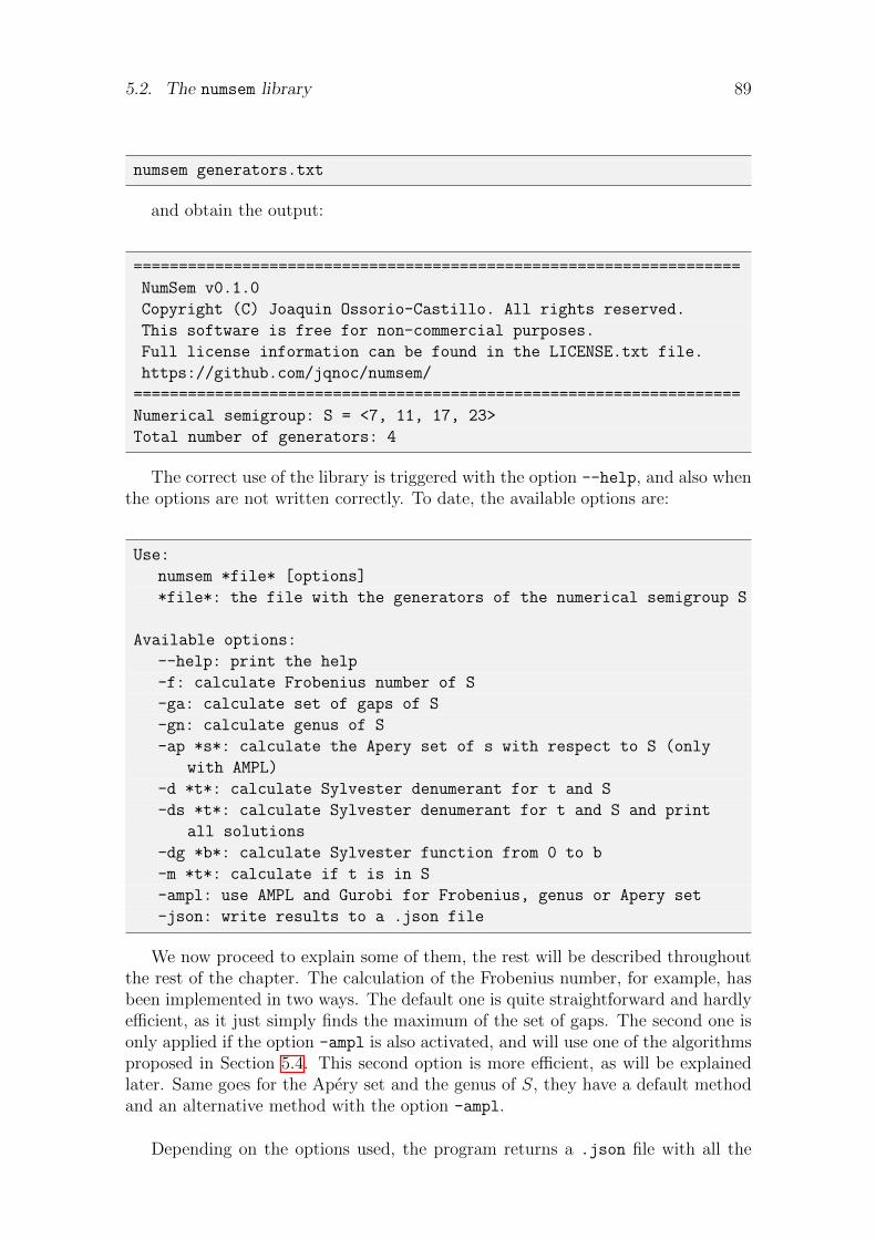
5.2. The numsem library 89
numsem generators.txt
and obtain the output:
===================================================================
NumSem v0.1.0
Copyright (C) Joaquin Ossorio-Castillo. All rights reserved.
This software is free for non-commercial purposes.
Full license information can be found in the LICENSE.txt file.
https://github.com/jqnoc/numsem/
===================================================================
Numerical semigroup: S = <7, 11, 17, 23>
Total number of generators: 4
The correct use of the library is triggered with the option --help, and also whenthe options are not written correctly. To date, the available options are:
Use:
numsem *file* [options]
*file*: the file with the generators of the numerical semigroup S
Available options:
--help: print the help
-f: calculate Frobenius number of S
-ga: calculate set of gaps of S
-gn: calculate genus of S
-ap *s*: calculate the Apery set of s with respect to S (only
with AMPL)
-d *t*: calculate Sylvester denumerant for t and S
-ds *t*: calculate Sylvester denumerant for t and S and print
all solutions
-dg *b*: calculate Sylvester function from 0 to b
-m *t*: calculate if t is in S
-ampl: use AMPL and Gurobi for Frobenius, genus or Apery set
-json: write results to a .json file
We now proceed to explain some of them, the rest will be described throughoutthe rest of the chapter. The calculation of the Frobenius number, for example, hasbeen implemented in two ways. The default one is quite straightforward and hardlyefficient, as it just simply finds the maximum of the set of gaps. The second one isonly applied if the option -ampl is also activated, and will use one of the algorithmsproposed in Section 5.4. This second option is more efficient, as will be explainedlater. Same goes for the Apery set and the genus of S, they have a default methodand an alternative method with the option -ampl.
Depending on the options used, the program returns a .json file with all the
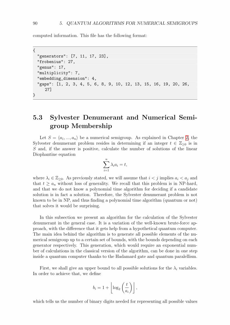
90 5. QUANTUM ALGORITHMS FOR NUMERICAL SEMIGROUPS
computed information. This file has the following format:
"generators": [7, 11, 17, 23],
"frobenius": 27,
"genus": 17,
"multiplicity": 7,
"embedding_dimension": 4,
"gaps": [1, 2, 3, 4, 5, 6, 8, 9, 10, 12, 13, 15, 16, 19, 20, 26,
27]
5.3 Sylvester Denumerant and Numerical Semi-
group Membership
Let S = 〈a1, ..., an〉 be a numerical semigroup. As explained in Chapter 2, theSylvester denumerant problem resides in determining if an integer t ∈ Z≥0 is inS and, if the answer is positive, calculate the number of solutions of the linearDiophantine equation
n∑i=1
λiai = t,
where λi ∈ Z≥0. As previously stated, we will assume that i < j implies ai < aj andthat t ≥ an without loss of generality. We recall that this problem is in NP-hard,and that we do not know a polynomial time algorithm for deciding if a candidatesolution is in fact a solution. Therefore, the Sylvester denumerant problem is notknown to be in NP, and thus finding a polynomial time algorithm (quantum or not)that solves it would be surprising.
In this subsection we present an algorithm for the calculation of the Sylvesterdenumerant in the general case. It is a variation of the well-known brute-force ap-proach, with the difference that it gets help from a hypothetical quantum computer.The main idea behind the algorithm is to generate all possible elements of the nu-merical semigroup up to a certain set of bounds, with the bounds depending on eachgenerator respectively. This generation, which would require an exponential num-ber of calculations in the classical version of the algorithm, can be done in one stepinside a quantum computer thanks to the Hadamard gate and quantum paralellism.
First, we shall give an upper bound to all possible solutions for the λi variables.In order to achieve that, we define
bi = 1 +
⌊log2
(t
ai
)⌋,
which tells us the number of binary digits needed for representing all possible values
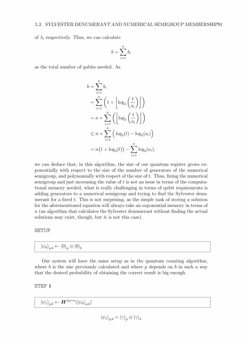
5.3. SYLVESTER DENUMERANT AND NUMERICAL SEMIGROUP MEMBERSHIP91
of λi respectively. Thus, we can calculate
b =n∑i=1
bi
as the total number of qubits needed. As
b =n∑i=1
bi
=n∑i=1
(1 +
⌊log2
(t
ai
)⌋)= n+
n∑i=1
(⌊log2
(t
ai
)⌋)≤ n+
n∑i=1
(log2(t)− log2(ai)
)= n
(1 + log2(t)
)−
n∑i=1
log2(ai),
we can deduce that, in this algorithm, the size of our quantum register grows ex-ponentially with respect to the size of the number of generators of the numericalsemigroup, and polynomially with respect of the size of t. Thus, fixing the numericalsemigroup and just increasing the value of t is not an issue in terms of the computa-tional memory needed, what is really challenging in terms of qubit requirements isadding generators to a numerical semigroup and trying to find the Sylvester denu-merant for a fixed t. This is not surprising, as the simple task of storing a solutionfor the aforementioned equation will always take an exponential memory in terms ofn (an algorithm that calculates the Sylvester denumerant without finding the actualsolutions may exist, though, but it is not this case).
SETUP
|ψ0〉p,b ← |0〉p ⊗ |0〉b
Our system will have the same setup as in the quantum counting algorithm,where b is the size previously calculated and where p depends on b in such a waythat the desired probability of obtaining the correct result is big enough.
STEP 1
|ψ1〉p,b ←H⊗p+n(|ψ0〉p,b)
|ψ1〉p,b = |γ〉p ⊗ |γ〉b

92 5. QUANTUM ALGORITHMS FOR NUMERICAL SEMIGROUPS
As has been already said, thanks to the Hadamard transformation we can obtainall computational basis states of our quantum system inside our register. As thedimension b is calculated with respect to the generators of the numerical semigroupand the integer t, these basis states correspond each one uniquely to a combinationfor all possible values of the variables λi. A representation of this feature is shownin Figure 5.1, where q1, q2, . . . , qb1 are the b1 binary digits of λi, and so on.
STEP 2
|ψ2〉p,b ← Cp,b(|ψ1〉p,b)
For the next step, we need the counting gate Cp,n, previously defined as
Cp,n : |m〉p ⊗ |ψ〉n → |m〉p ⊗ (Gn)m |ψ〉n ,
where Gn is again the Grover gate. This Grover gate depends in turn on the Oraclegate Of used in the algorithms described in Chapter 4, and yields the followingresult when applied to a basis state:
Of : |j〉n ⊗ |k〉m → |j〉n ⊗ |k ⊕ f(j)〉m .
We recall that the oracle gate is problem specific, and depends on a certainfunction f capable of recognising a solution for our problem. What we are goingto do is to define f in such a way that it identifies if a certain combination ofthe variables λi encoded into our quantum register are a solution for the numericalsemigroup membership problem. In other words:
f(j) =
1 ifn∑i=1
λiai = t
0 otherwise
The rest of the algorithm continues as previously explained, but what interestsus now is the size of the first register, p, which depends on b but also on the prob-ability of obtaining the correct solution for the Sylvester denumerant. Thanks to[28] and [29], we know that in order to have a reasonable probability of succeeding,
p ∼√
2b. Thus, the computational order of the algorithm remains the same in bothmemory size and time.
Concerning the performance of the algorithm, let us compare the iterationsrequired for the brute force approach to calculate the Sylvester denumerant fora fixed semigroup and an increasing value of t, against the hypothetical perfor-mance of the quantum variant. Let S = 〈376, 381, 393, 399〉 be a numerical semi-group and let t = 10000, we can calculate d(10000; 376, 381, 393, 399) with the
λ1 λ2 · · · λn
q1 q2 · · · · · · qbqb1 qb1+1 qb1+b2· · · qbn−1+1
Figure 5.1: Representation of the values of λi with respect to the b qubits
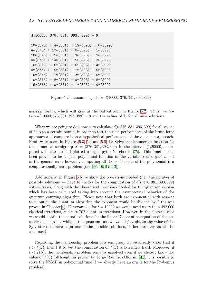
5.3. SYLVESTER DENUMERANT AND NUMERICAL SEMIGROUP MEMBERSHIP93
d(10000; 376, 381, 393, 399) = 9
10*(376) + 4*(381) + 12*(393) + 0*(399)
4*(376) + 13*(381) + 8*(393) + 1*(399)
10*(376) + 5*(381) + 9*(393) + 2*(399)
4*(376) + 14*(381) + 5*(393) + 3*(399)
10*(376) + 6*(381) + 6*(393) + 4*(399)
4*(376) + 15*(381) + 2*(393) + 5*(399)
10*(376) + 7*(381) + 3*(393) + 6*(399)
10*(376) + 8*(381) + 0*(393) + 8*(399)
16*(376) + 0*(381) + 1*(393) + 9*(399)
Figure 5.2: numsem output for d(10000; 376, 381, 393, 399)
numsem library, which will give us the output seen in Figure 5.2. Thus, we ob-tain d(10000; 376, 381, 393, 399) = 9 and the values of λi for all nine solutions.
What we are going to do know is to calculate d(t; 376, 381, 393, 399) for all valuesof t up to a certain bound, in order to test the time performance of the brute-forceapproach and compare it to a hypothetical performance of the quantum approach.First, we can see in Figures 5.3, 5.4 and 5.5 the Sylvester denumerant function forthe numerical semigroup S = 〈376, 381, 393, 399〉 in the interval (1,20000), com-puted with numsem and plotted using Jupyter Notebooks [75]. This function hasbeen proven to be a quasi-polynomial function in the variable t of degree n − 1in the general case; however, computing all the coefficients of the polynomial is acomputationally hard problem (see [98, 16, 17, 13]).
Additionally, in Figure 5.6 we show the operations needed (i.e., the number ofpossible solutions we have to check) for the computation of d(t; 376, 381, 393, 399)with numsem, along with the theoretical iterations needed for the quantum versionwhich has been calculated taking into account the asymptotical behavior of thequantum counting algorithm. Please note that both are exponential with respectto t, but in the quantum algorithm the exponent would be divided by 2 (as wasproven in Chapter 4). For example, for t = 10000 we would need more than 492,000classical iterations, and just 702 quantum iterations. However, in the classical casewe would obtain the actual solutions for the linear Diophantine equation of the nu-merical semigroup, while in the quantum case we would just obtain the value of theSylvester denumerant (or one of the possible solutions, if there are any, as will beseen now).
Regarding the membership problem of a semigroup S, we already know that ift > f(S), then t ∈ S, but the computation of f(S) is extremely hard. Moreover, ift < f(S), the membership problem remains unsolved even if we already know thevalue of f(S) (although, as proven by Jorge Ramırez-Alfonsın [97], it is possible tosolve the NSMP in polynomial time if we already have an oracle for the Frobeniusproblem).

94 5. QUANTUM ALGORITHMS FOR NUMERICAL SEMIGROUPS
Figure 5.3: Sylvester quasi-polynomial
Figure 5.4: Sylvester quasi-polynomial (detail)
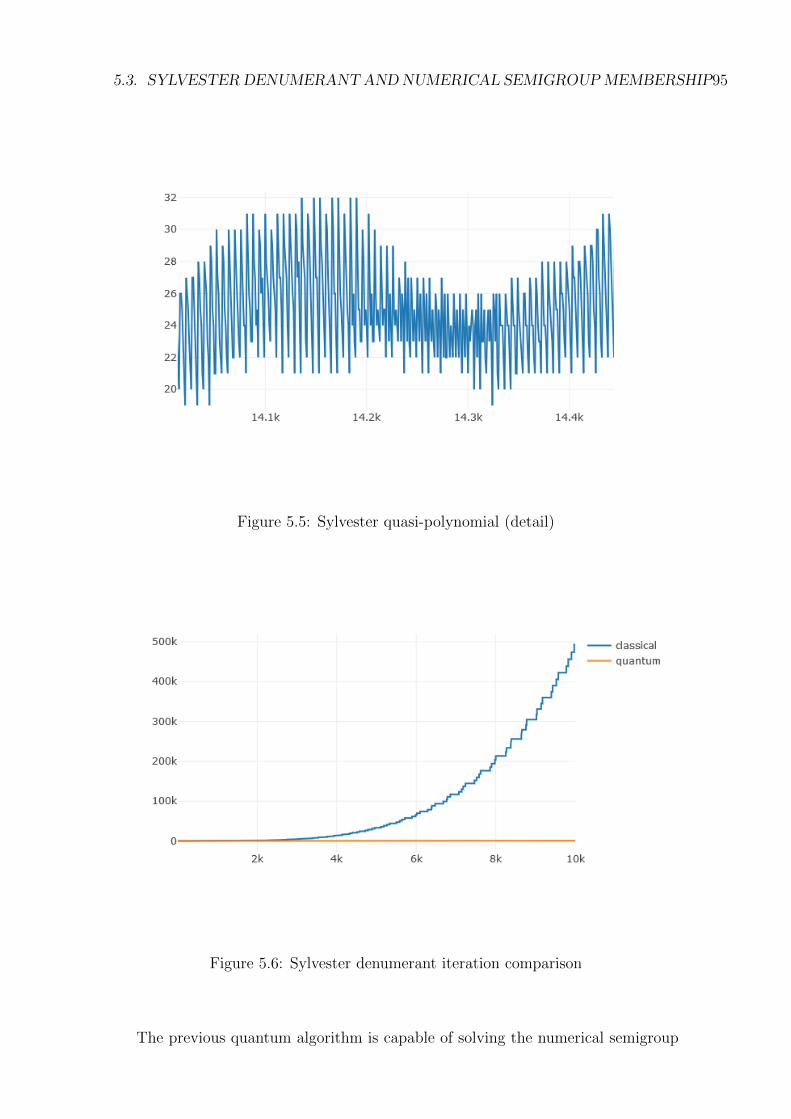
5.3. SYLVESTER DENUMERANT AND NUMERICAL SEMIGROUP MEMBERSHIP95
Figure 5.5: Sylvester quasi-polynomial (detail)
Figure 5.6: Sylvester denumerant iteration comparison
The previous quantum algorithm is capable of solving the numerical semigroup

96 5. QUANTUM ALGORITHMS FOR NUMERICAL SEMIGROUPS
membership problem for a certain t ∈ Z≤0. We have to just calculate the SylvesterDenumerant for t and, if d(S; t) > 0 return YES and otherwise return NO. This isquite straightforward but, how about solving the NSMP constructively, not onlyanswering YES or NO to the question of whether there exist those λi, . . . , λn, but alsogiving one of its possible combinations if the answer is YES. For that purpose, wewill make use of Grover’s Quantum Search algorithm, already explained in Section4.6.
Using Grover’s Algorithm, we can provide a solution for the NSMP linear Dio-phantine equation in the same
√2b steps as for the Sylvester denumerant. The
actual order of both algorithms with respect to t, the number of generators n of thenumerical semigroup, and the generators a1, . . . , an is:√
2n(
1+log2(t))−∑ni=1 log2(ai)
We can also go further and obtain all solutions to the Diophantine equation.First, we run the quantum algorithm for the Sylvester denumerant. Then, we applythe quantum algorithm for the NSMP iteratively until we have obtained as muchdifferent solutions as the value of the denumerant. This is a well-known problem inprobability theory [51] known as the coupon collector’s problem; if the denumerantis d, then the expected number of trials k ≥ d for obtaining all d solutions grows as
Θ(d log(d)).
For example, if d = 10, the expected number of runs of the quantum algorithm forthe NSMP before obtaining all different solutions is 33.
5.4 Apery Set and Frobenius Problem
The next algorithm shows the possibilities of calculating the Apery set and theFrobenius number of a numerical semigroup with an actual adiabatic quantum com-puter. As described in Section 3.5, current D-Wave quantum annealers solve acertain kind of mathematical optimization problems known as Ising spin problems,namely
H(s1, . . . , sn) =n∑i=1
hisi +n−1∑i=1
n∑j=i+1
Jijsisj
with si ∈ −1, 1, where the objective is to find the minimum of H(s1, . . . , sn).
On the other hand, we recall that the Apery set with respect to s ∈ S \ 0,where S = 〈a1, . . . , an〉 is a numerical semigroup, is defined as
Ap(S, s) = x ∈ S | x− s /∈ S.
The question is, how could we be able to translate this problem to the Ising spinmodel solved by the D-Wave machine? We have already proved in Lemma 2.1.11that Ap(S, s) = ω0, . . . , ωn−1, where
ωi = minx ∈ S : x ≡ i mod s.

5.4. APERY SET AND FROBENIUS PROBLEM 97
How about transforming the definition of ωi into the answer of a mathematical op-timization problem?
Definition 5.4.1. [93] An integer linear program, or ILP, is defined in its canonicalform as the optimization problem:
min cTxsubject to: Ax = b
where x ∈ Zn≥0, A ∈ Zn × Zm, b ∈ Zm and c ∈ Zn.
Thus, it is straightforward to see that the calculation of each of the ωi can beredefined as the following ILP:
minn∑j=1
ajxj
subject to:n∑j=1
ajxj = i+ sk,
with xj ∈ Z≥0 for all j = 1, ..., n and k ∈ Z≥0.
This mathematical optimization problem represents a way of calculating theApery set in its own right and, although integer linear programming is in NP-hardand its recognition version (deciding whether Ax = b has a feasible solution or notregardless of its optimality) is in NP-complete [93], this computational complexityarises in the general case. In our context, it may prove to be an easier problem; how-ever, details on this remain to be worked out. This approach for the calculation ofthe Apery set first appeared in [61], although Greenberg’s work dealt with the directcalculation of the Frobenius number by means of Ap(S, a1), as will be discussed later.
We have tested this algorithm using state-of-the-art optimization software forinteger optimization. In our case, the optimization problem for ωi was modeledusing AMPL [53, 54], an algebraic modeling language for solving mathematicaloptimization problems. AMPL has a clear advantage, as our problem is entirelyparameterized and AMPL allows us to describe the generic problem in a .mod filewhile defining the actual values for the parameters in a separate .dat file. Thisway, we have just to change the parameters inside the .dat file in order to solvea new instance of the Apery set. The .mod file we propose is shown in Figure 5.7(the names of the parameters and variables of the problem are maintained so thatno further explanation is required).
Let us suppose that we are interested in the numerical semigroup S = 〈11, 19, 23〉,and that we want to calculate the Apery set of s = 30 (i.e., Ap(S, 30)). The cal-culation of, for example, ω5 ∈ Ap(S, 30), will have the associated .dat file depictedin Figure 5.8. In order to compute ω5, we also need a .run file that will load themodel and the data of the problem, and which will also call the solver for solvingthe problem. In our case, the solver we have chosen is Gurobi [3] which, among

98 5. QUANTUM ALGORITHMS FOR NUMERICAL SEMIGROUPS
other things, solves integer linear problems up to a global optimum. The .run filewe have used is shown in Figure 5.9, and the corresponding output we obtain can beseen in Figure 5.10. This output tells us that ω5 = 65 and also that a representationof 65 with respect to the generators of the semigroup is
65 = 0× (11) + 1× (19) + 2× (23).
We can also write an alternative .run file that will directly calculate and display
param n;
set N := 1..n;
param a N;
param s;
param i;
var X N integer, >= 0;
var K integer;
minimize T:
sum j in N a[j]*X[j];
subject to C:
sum j in N a[j]*X[j] = i + s*K;
Figure 5.7: File apery_set_member.mod
param n := 3;
param a :=
1 11
2 19
3 23;
Figure 5.8: File numerical_semigroup.dat
model apery_set_member.mod;
data numerical_semigroup.dat;
let s := 30;
let i := 5;
option solver gurobi;
solve;
display X;
display K;
Figure 5.9: File apery_set_member.run

5.4. APERY SET AND FROBENIUS PROBLEM 99
the whole content of the Apery set for a certain s ∈ S. First, we have to dropthe param i := 5; line from the .run file, as it will be changed in each iterationof the main loop, and modify the .run so that it will look like the one in Figure5.11. Thus, we obtain Ap(S, 30) = 0, 11, 19, 22, 23, 33, 34, 38, 42, 44, 45, 46, 55, 56,57, 61, 65, 66, 67, 69, 77, 78, 80, 84, 88, 89, 92, 100, 103, 111 (see Figure 5.12 for the ac-tual output).
This algorithm also provides a way for calculating the Frobenius number of a
Gurobi 8.0.0: optimal solution; objective 65
3 simplex iterations
1 branch-and-cut nodes
X [*] :=
1 0
2 1
3 2
;
K = 2
Figure 5.10: Output for apery_set_member.run
model apery_set_member.mod;
data numerical_semigroup.dat;
let s := 30;
option solver gurobi;
param apery_set 0..s-1;
for l in 0..s-1
let i := l;
solve;
let apery_set[l] := T;
display apery_set;
Figure 5.11: File apery_set.run
apery_set [*] :=
0 0 4 34 8 38 12 42 16 46 20 80 24 84 28 88
1 61 5 65 9 69 13 103 17 77 21 111 25 55 29 89
2 92 6 66 10 100 14 44 18 78 22 22 26 56
3 33 7 67 11 11 15 45 19 19 23 23 27 57
;
Figure 5.12: Output for apery_set.run
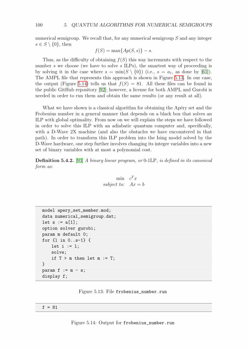
100 5. QUANTUM ALGORITHMS FOR NUMERICAL SEMIGROUPS
numerical semigroup. We recall that, for any numerical semigroup S and any integers ∈ S \ 0, then
f(S) = maxAp(S, s) − s.
Thus, as the difficulty of obtaining f(S) this way increments with respect to thenumber s we choose (we have to solve s ILPs), the smartest way of proceeding isby solving it in the case where s = min(S \ 0) (i.e., s = a1, as done by [61]).The AMPL file that represents this approach is shown in Figure 5.13. In our case,the output (Figure 5.14) tells us that f(S) = 81. All these files can be found inthe public GitHub repository [92]; however, a license for both AMPL and Gurobi isneeded in order to run them and obtain the same results (or any result at all).
What we have shown is a classical algorithm for obtaining the Apery set and theFrobenius number in a general manner that depends on a black box that solves anILP with global optimality. From now on we will explain the steps we have followedin order to solve this ILP with an adiabatic quantum computer and, specifically,with a D-Wave 2X machine (and also the obstacles we have encountered in thatpath). In order to transform this ILP problem into the Ising model solved by theD-Wave hardware, one step further involves changing its integer variables into a newset of binary variables with at most a polynomial cost.
Definition 5.4.2. [93] A binary linear program, or 0-1LP, is defined in its canonicalform as:
min cTxsubject to: Ax = b
model apery_set_member.mod;
data numerical_semigroup.dat;
let s := a[1];
option solver gurobi;
param m default 0;
for l in 0..s-1
let i := l;
solve;
if T > m then let m := T;
param f := m - s;
display f;
Figure 5.13: File frobenius_number.run
f = 81
Figure 5.14: Output for frobenius_number.run
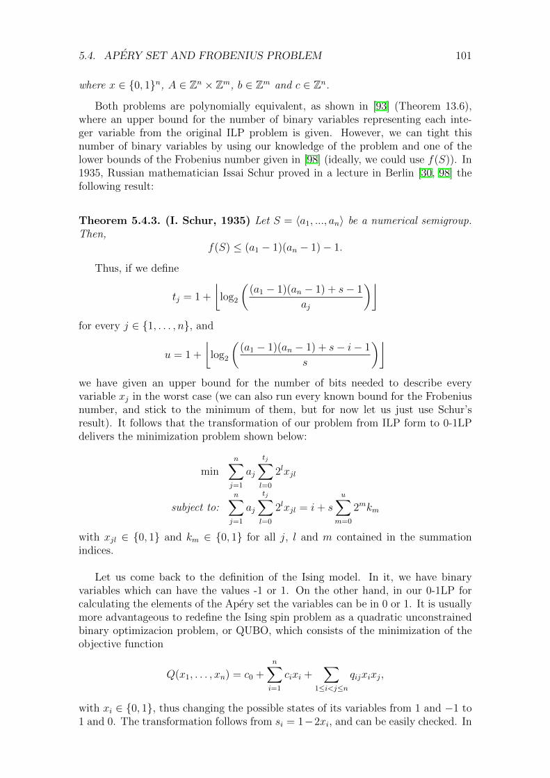
5.4. APERY SET AND FROBENIUS PROBLEM 101
where x ∈ 0, 1n, A ∈ Zn × Zm, b ∈ Zm and c ∈ Zn.
Both problems are polynomially equivalent, as shown in [93] (Theorem 13.6),where an upper bound for the number of binary variables representing each inte-ger variable from the original ILP problem is given. However, we can tight thisnumber of binary variables by using our knowledge of the problem and one of thelower bounds of the Frobenius number given in [98] (ideally, we could use f(S)). In1935, Russian mathematician Issai Schur proved in a lecture in Berlin [30, 98] thefollowing result:
Theorem 5.4.3. (I. Schur, 1935) Let S = 〈a1, ..., an〉 be a numerical semigroup.Then,
f(S) ≤ (a1 − 1)(an − 1)− 1.
Thus, if we define
tj = 1 +
⌊log2
((a1 − 1)(an − 1) + s− 1
aj
)⌋for every j ∈ 1, . . . , n, and
u = 1 +
⌊log2
((a1 − 1)(an − 1) + s− i− 1
s
)⌋we have given an upper bound for the number of bits needed to describe everyvariable xj in the worst case (we can also run every known bound for the Frobeniusnumber, and stick to the minimum of them, but for now let us just use Schur’sresult). It follows that the transformation of our problem from ILP form to 0-1LPdelivers the minimization problem shown below:
minn∑j=1
aj
tj∑l=0
2lxjl
subject to:n∑j=1
aj
tj∑l=0
2lxjl = i+ su∑
m=0
2mkm
with xjl ∈ 0, 1 and km ∈ 0, 1 for all j, l and m contained in the summationindices.
Let us come back to the definition of the Ising model. In it, we have binaryvariables which can have the values -1 or 1. On the other hand, in our 0-1LP forcalculating the elements of the Apery set the variables can be in 0 or 1. It is usuallymore advantageous to redefine the Ising spin problem as a quadratic unconstrainedbinary optimizacion problem, or QUBO, which consists of the minimization of theobjective function
Q(x1, . . . , xn) = c0 +n∑i=1
cixi +∑
1≤i<j≤n
qijxixj,
with xi ∈ 0, 1, thus changing the possible states of its variables from 1 and −1 to1 and 0. The transformation follows from si = 1−2xi, and can be easily checked. In

102 5. QUANTUM ALGORITHMS FOR NUMERICAL SEMIGROUPS
fact, the documentation from D-Wave allows to program our problem directly intoa QUBO formulation [1], besides the Ising model formulation. One detail remainsto be figured out: QUBO problems have no constraints, but ours have one. How toproceed?
The most common way to transform a constrained optimization problem into anunconstrained one is by penalizing the constraints, putting them in the objectivefunction. In this manner, we can force the fulfillment of the constraints of theproblem by punishing the error committed in them. In our example, as we have asingle equality constraint, namely
n∑j=1
ajxj = i+ sk,
we can force it to the objective function this way:
minn∑j=1
ajxj + λ(ν)
(n∑j=1
ajxj − i− sk
)2
where λ(ν) is updated after every iteration in the following way, until no change inλ is obtained:
λ(ν+1) = λ(ν) + α ·
∣∣∣∣∣n∑j=1
ajxj − i− sk
∣∣∣∣∣with α > 0.
In 0-1LP form, we obtain the following QUBO problem:
minn∑j=1
aj
tj∑l=0
2lxjl + λ(ν)
(n∑j=1
aj
tj∑l=0
2lxjl − i− su∑
m=0
2mkm
)2
,
with its corresponding penalty updating formula:
λ(ν+1) = λ(ν) + α ·
∣∣∣∣∣n∑j=1
aj
tj∑l=0
2lxjl − i− su∑
m=0
2mkm
∣∣∣∣∣with α > 0.
Now, we are going to test the performance of this new procedure for obtain-ing the Apery set (and the Frobenius number) via a classical solver. For that, wehave just to modify the original apery_set_member.mod file into a new one withan unconstrained ILP, with the constraint penalized in the objective function aspreviously exaplained. This new AMPL file can be found in Figure 5.15, along withits corresponding .run file in Figure 5.16. Additionaly, we are going to keep track ofthe number of iterations of the algorithm (i.e., ν), and on the values of λ(ν) neededfor the algorithm to stop. This way, if we start with λ(0) = 0, the output for thisalgorithm is found in Figure 5.17. On the other hand, if we start with λ(0) = 100,

5.4. APERY SET AND FROBENIUS PROBLEM 103
param n;
set N := 1..n;
param a N;
param s; #
param i; #
param lambda;
param rest;
var X N integer, >= 0;
var K integer;
minimize T:
sum j in N a[j]*X[j]
+ lambda*((sum j in N a[j]*X[j] - i - s*K)^2);
Figure 5.15: File apery_set_member_lagr.mod
the output is shown in Figure 5.18.
Foreseeably, the Apery set we obtain for S and s = 30 is correct, but that shouldnot be a surprise as both optimization problems are equivalent to the original one.What is of interest here is that a low starting point for λ implies a relatively largenumber of iterations, which translates in more calls to our integer linear program-ming solver than in the original constrained version. However, if we start with alarge enough value of λ, we can obtain the same results without additional calls tothe solver and just one iterarion for each of the elements of the Apery set. On theother hand, if we exceed in the value for λ, we would also need just one iterationper ωi, but the solver would need more time in order to find the global optimum.The latter behavior can be observed when taking into account the number of sim-plex iterarions and branch-and-cut nodes that Gurobi needs for each of the problems.
Nevertheless, this unconstrained reformulation of the problem is not meant to besolved by Gurobi or any other integer linear programming solver, but rather by anideal adiabatic quantum computer, and more concretely by one of the few D-Wavemachines that currently exist worldwide. Our unconstrained problem, in QUBOform, is shown below (please note that, if x ∈ 0, 1, then x = x2):
c0 +u∑
m=0
cmkm +n∑j=1
(tj∑l=0
cjlxjl
)+
∑1≤j<j′≤n
∑0≤l<l′≤min(tj ,tj′ )
iqjl,j′l′xjlxj′l′
+n∑j=1
[tj∑l=0
(u∑
m=0
qjl,mxjlkm
)]+
∑0≤m<m′≤u
qm,m′ ,
where

104 5. QUANTUM ALGORITHMS FOR NUMERICAL SEMIGROUPS
c0 = λ(ν)i2
cm = λ(ν) (22ms2 + 2m+1is)cjl = 2laj + λ(ν)
(22la2
j − 2l+1aji)
qm,m′ = 2m+m′+1λ(ν)s2
qjl,m = 2l+m+1λ(ν)ajsqjl,j′l′ = 2l+l
′+1λ(ν)ajaj′ .
Right now, an ideal quantum annealer should be able to solve our QUBO prob-lem for finding the members of the Apery set, provided that such a computer hasa sufficiently large enough amount of qubits, and also that the graph connectingthe qubits is complete. However, to date there are no quantum annealers that ful-fill those requirements (they may be available in the future, though). The latestquantum annealers commercially available are the D-Wave 2X, with 1152 and 3360couplers (connections between adjacent qubits), and the D-Wave 2000Q, which has2048 qubits and 6016 couplers. Their graphs are far from being complete, as every
model apery_set_member_lagr.mod;
data numerical_semigroup.dat;
let s := 30;
param apery_set 0..s-1;
param lambdas 0..s-1;
param iterations 0..s-1;
param it default 0;
option solver gurobi;
for l in 0..s-1
let i := l;
let lambda := 0;
let it := 0;
let rest := 1;
repeat
solve;
let rest := abs(sum j in N a[j]*X[j] - i - s*K);
let lambda := lambda + rest;
let it := it + 1;
while rest != 0;
let apery_set[l] := T;
let lambdas[l] := lambda;
let iterations[l] := it;
display apery_set;
display iterations;
display lambdas;
Figure 5.16: File apery_set_lagr.run

5.4. APERY SET AND FROBENIUS PROBLEM 105
qubit in their grids are at most connected with six other qubits, as shown in Figure
apery_set [*] :=
0 0 4 34 8 38 12 42 16 46 20 80 24 84 28 88
1 61 5 65 9 69 13 103 17 77 21 111 25 55 29 89
2 92 6 66 10 100 14 44 18 78 22 22 26 56
3 33 7 67 11 11 15 45 19 19 23 23 27 57
;
iterations [*] :=
0 1 3 2 6 2 9 2 12 22 15 2 18 2 21 11 24 40 27 2
1 63 4 2 7 2 10 22 13 21 16 2 19 2 22 2 25 2 28 2
2 2 5 2 8 2 11 2 14 2 17 2 20 44 23 2 26 2 29 3
;
lambdas [*] :=
0 0 4 34 8 68 12 32 16 46 20 62 24 62 28 58
1 62 5 35 9 39 13 62 17 47 21 90 25 85 29 90
2 62 6 66 10 90 14 104 18 78 22 112 26 56
3 93 7 67 11 101 15 45 19 79 23 23 27 57
;
Figure 5.17: Output for apery_set_lagr.run and λ(0) = 0
apery_set [*] :=
0 0 4 34 8 38 12 42 16 46 20 80 24 84 28 88
1 61 5 65 9 69 13 103 17 77 21 111 25 55 29 89
2 92 6 66 10 100 14 44 18 78 22 22 26 56
3 33 7 67 11 11 15 45 19 19 23 23 27 57
;
iterations [*] :=
0 1 3 1 6 1 9 1 12 1 15 1 18 1 21 1 24 1 27 1
1 1 4 1 7 1 10 1 13 1 16 1 19 1 22 1 25 1 28 1
2 1 5 1 8 1 11 1 14 1 17 1 20 1 23 1 26 1 29 1
;
lambdas [*] :=
0 100 4 100 8 100 12 100 16 100 20 100 24 100 28 100
1 100 5 100 9 100 13 100 17 100 21 100 25 100 29 100
2 100 6 100 10 100 14 100 18 100 22 100 26 100
3 100 7 100 11 100 15 100 19 100 23 100 27 100
;
Figure 5.18: Output for apery_set_lagr.run and λ(0) = 100
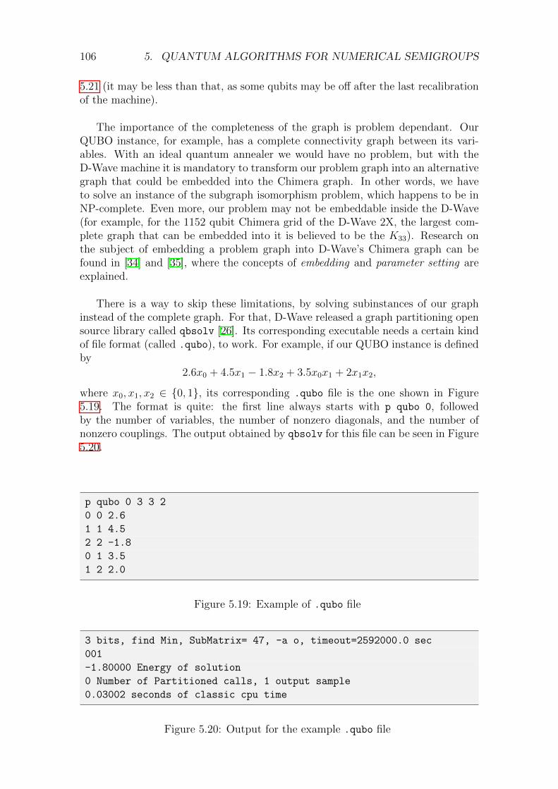
106 5. QUANTUM ALGORITHMS FOR NUMERICAL SEMIGROUPS
5.21 (it may be less than that, as some qubits may be off after the last recalibrationof the machine).
The importance of the completeness of the graph is problem dependant. OurQUBO instance, for example, has a complete connectivity graph between its vari-ables. With an ideal quantum annealer we would have no problem, but with theD-Wave machine it is mandatory to transform our problem graph into an alternativegraph that could be embedded into the Chimera graph. In other words, we haveto solve an instance of the subgraph isomorphism problem, which happens to be inNP-complete. Even more, our problem may not be embeddable inside the D-Wave(for example, for the 1152 qubit Chimera grid of the D-Wave 2X, the largest com-plete graph that can be embedded into it is believed to be the K33). Research onthe subject of embedding a problem graph into D-Wave’s Chimera graph can befound in [34] and [35], where the concepts of embedding and parameter setting areexplained.
There is a way to skip these limitations, by solving subinstances of our graphinstead of the complete graph. For that, D-Wave released a graph partitioning opensource library called qbsolv [26]. Its corresponding executable needs a certain kindof file format (called .qubo), to work. For example, if our QUBO instance is definedby
2.6x0 + 4.5x1 − 1.8x2 + 3.5x0x1 + 2x1x2,
where x0, x1, x2 ∈ 0, 1, its corresponding .qubo file is the one shown in Figure5.19. The format is quite: the first line always starts with p qubo 0, followedby the number of variables, the number of nonzero diagonals, and the number ofnonzero couplings. The output obtained by qbsolv for this file can be seen in Figure5.20.
p qubo 0 3 3 2
0 0 2.6
1 1 4.5
2 2 -1.8
0 1 3.5
1 2 2.0
Figure 5.19: Example of .qubo file
3 bits, find Min, SubMatrix= 47, -a o, timeout=2592000.0 sec
001
-1.80000 Energy of solution
0 Number of Partitioned calls, 1 output sample
0.03002 seconds of classic cpu time
Figure 5.20: Output for the example .qubo file

5.4. APERY SET AND FROBENIUS PROBLEM 107
Figure 5.21: Introducing a problem inside the D-Wave 2X
Please note that, in the previous paragraph, we have shown the solution thatqbsolv obtains for a certain instance of the problem. This is because qbsolv hasan auxiliary internal optimization solver based on the tabu search [58], which givesa solution for the subproblems and then unifies all the solutions into the completeone for all the variables. However, this classical method does not guarantee a globalsolution, and is of no help to us in the general case. We can decide if qbsolv triesto solve the problem with its tabu search, of if we prefer to connect to a D-Wavemachine.
Finally, our QUBO subproblem is solved with the D-Wave 2X via one of thepossible inputs allowed. The first one is shown in Figure 5.21, while the second oneis again a .qubo file obtained internally with qbsolv. As part of the project JointResearch Unit Repsol-ITMATI (code file: IN853A 2014/03), we had the opportu-nity to try the D-Wave 2X machine based on the University of Southern California.However, due to the amount of subproblems needed to solve a proper instance ofthe Frobenius problem or the Apery set, it was impractical to do so with the scarceamount of time given and the current size of the graph of the D-Wave 2X machine.In the last chapter we discuss the conclusions at which we arrived during the process.

108 5. QUANTUM ALGORITHMS FOR NUMERICAL SEMIGROUPS
6
Conclusions and Future Work
What we have presented in this doctoral dissertation is a preliminary study of thecapabilities of quantum computation when it comes to solve numerical semigroup-related problems. In order to do that, we have first defined what numerical semi-groups are, and then, drawing upon the principles of computational complexitytheory, we prove that the problems we want to answer with hypothetical quantumcomputers are in fact hard to solve. Thus, this work is a first attempt at solvingone of the most computationally demanding problems in basic algebra with thisemerging and somewhat promising computing paradigm. As have been explained,calculating the Sylvester denumerant and the Frobenius number of a numerical semi-group are not even known to be in the computational class NP (i.e., just deciding ifa certain integer is the Frobenius number or the Sylvester denumerant is a challegingproblem).
With that in mind, it is important to clarify that we did not expect in any mo-ment to find polynomial-time quantum algorithms for those problems. As with theSankara stones, doing so would have triggered a series of actions that would haveeventually led us to never-ending fortune and glory. It is also important to take intoaccount that quantum computing is not a panacea for computationally hard prob-lems. In fact, there are not many problems that have quantum algorithms fasterthan their classical counterparts (without the involvement of oracles). Even more,in those few special cases it remains to be proven yet that a classical algorithm com-parable to the quantum one in terms of efficiency does not exist. The best exampleis Shor’s algorithm: right now, it is the only known polynomial time algorithm forthe factoring problem; however, even though the general number field sieve (i.e.,the most efficient classical factoring algorithm) is super-polynomial, it has not beenproven that there are no classical polynomial factoring algorithms. Proving so willanswer the question of whether there are NP problems not in P.
During these years we have also followed a lead (unrelated to quantum comput-ing) that, if finally proven true, would strengthen the hard nature of the Frobeniusproblem. There exist the possibility that the Frobenius number is not just one ofthe problems in the class NP-hard, but also a problem in the class PSPACE-hard(please note that NP ⊆ PSPACE and that the equality, although not properly dis-carded yet, would be startling). Details of this remain, however, to be worked outyet; due to time limitations we did not arrive to any definite —and, of course, math-
109

110 6. CONCLUSIONS AND FUTURE WORK
ematically proven— conclusion during the span of this doctoral dissertation.
As with quantum computing, to date the only algorithm that is proven to bestrictly more efficient that its classical counterpart is Grover’s Search. However, inorder to use this algorithm, one must have a way of identifying in a reasonable time(i.e., polynomial with respect to the size of the input) whether a possible solutionis in fact a solution. This, of course, limits its usage to problems in the class NP,and is the reason why we have solved the Sylvester denumerant problem with thehelp of an oracle for the NSMP. There exists, however, the possibility that power-ful quantum gate algorithms exist in their own right for the Sylvester denumerant(without having to find the actual solutions for the NSMP) and also for the Frobe-nius problem, but the search must continue from this point. The lack of results sinceShor and Grover gave birth to their clever ideas is, nonetheless, discouraging, andmay be an indicative that the only advantage of quantum computers with respectto classical ones would and ever would be a quadratic speedup in database searches.Furthermore, there are other problems that arise when trying to construct a quan-tum computer in practice; we have not covered them here, but we refere to [6] for abrief and clever introduction.
Regarding the algorithms for the Apery set and the Frobenius number, there aretwo aspects that need to be improved prior to completing a study of its feasibil-ity and performance. First, the current graph (i.e., Chimera graph) architecture ofthe available adiabatic quantum computers (i.e., the D-Wave machines) extremelyobstruct the resolution of problems that have an almost full connectivity index be-tween its variables, as in this case (the use of qbsolv is just a temporary workaround,or it should be as so). And second, current adiabatic quantum computers do notguarantee global optimality, as opposed to the theoretical result deducted fromthe adiabatic theorem; in reality, the D-Wave just make a few runs of the process(instead of just one, as would be in the theoretical case) and, following a certainprobability distribution, try to guarantee that the best of the solutions obtained bythose runs is in fact the global solution to the problem. This solution, however,cannot be proven to be the global optimum (as global optimality is not known to bein the class NP), which makes useless our attempt to find those two combinatorialinvariants via current adiabatic quantum computers. In the future, with more reli-able quantum annealers, however, this solution may prove to be effective and faster,but for now it is just a theoretical method.

7
Bibliography
[1] D-Wave: Programming with QUBOs. Release 1.5.1-beta4, 09-1002A-B., tech.rep., D-Wave Systems, Inc., 2016.
[2] D-Wave: Programming with QUBOs. Release 2.3, 09-1002A-B., tech. rep.,D-Wave Systems, Inc., 2016.
[3] Gurobi Optimizer Reference Manual. http://www.gurobi.com, 2018. Ac-cessed: 2019-02-23.
[4] S. Aaronson, P?= NP , in Open Problems in Mathematics, Springer, 2016,
pp. 1–122.
[5] S. Aaronson, G. Kuperberg, and C. Granade, The Complexity Zoo.https://complexityzoo.uwaterloo.ca/Complexity_Zoo, 2005. Accessed:2017-04-25.
[6] S. Aaronson and Z. Weinersmith, The Talk. http://www.smbc-comics.com/comic/the-talk-3, 2016. Accessed: 2019-03-03.
[7] M. Agrawal, N. Kayal, and N. Saxena, PRIMES is in P, Annals ofMathematics, 160 (2004), pp. 781–793.
[8] D. Aharonov, W. Van Dam, J. Kempe, Z. Landau, S. Lloyd, andO. Regev, Adiabatic quantum computation is equivalent to standard quantumcomputation, SIAM Review, 50 (2008), pp. 755–787.
[9] T. Albash and D. A. Lidar, Adiabatic quantum computation, Reviews ofModern Physics, 90 (2018), p. 015002.
[10] R. Apery, Geometrie algebrique - sur les branches superlineaires des courbesalgebriques, Comptes Rendus Hebdomadaires des Seances de l’Academie desSciences, 222 (1946), pp. 1198–1200.
[11] , Irrationalite de ζ (2) et ζ (3), Asterisque, 61 (1979), p. 1.
[12] B. Aspvall and R. E. Stone, Khachiyan’s linear programming algorithm,Journal of Algorithms, 1 (1980), pp. 1–13.
111

112 7. BIBLIOGRAPHY
[13] V. Baldoni, N. Berline, J. De Loera, B. Dutra, M. Koeppe,and M. Vergne, Coefficients of Sylvester’s denumerant, arXiv preprintarXiv:1312.7147, (2013).
[14] F. Barahona, On the computational complexity of Ising spin glass models,Journal of Physics A: Mathematical and General, 15 (1982), p. 3241.
[15] A. Barenco, C. H. Bennett, R. Cleve, D. P. DiVincenzo, N. Mar-golus, P. Shor, T. Sleator, J. A. Smolin, and H. Weinfurter,Elementary gates for quantum computation, Physical Review A, 52 (1995),p. 3457.
[16] M. Beck, I. M. Gessel, and T. Komatsu, The polynomial part of arestricted partition function related to the Frobenius problem, The ElectronicJournal of Combinatorics, 8 (2001), p. 7.
[17] E. Bell, Interpolated denumerants and Lambert series, American Journal ofMathematics, 65 (1943), pp. 382–386.
[18] J. S. Bell, On the Einstein Podolsky Rosen paradox, Physics, 1 (1964),pp. 195–200.
[19] P. Benioff, The computer as a physical system: a microscopic quantum me-chanical Hamiltonian model of computers as represented by Turing machines,Journal of Statistical Physics, 22 (1980), pp. 563–591.
[20] C. H. Bennett, E. Bernstein, G. Brassard, and U. Vazirani,Strengths and weaknesses of quantum computing, SIAM Journal on Comput-ing, 26 (1997), pp. 1510–1523.
[21] D. J. Bernstein and A. K. Lenstra, A general number field sieve imple-mentation, in The Development of the Number Field Sieve, Springer, 1993,pp. 103–126.
[22] E. Bernstein and U. Vazirani, Quantum complexity theory, SIAM Journalon Computing, 26 (1997), pp. 1411–1473.
[23] E. Bezout, Theorie generale des equations algebriques; par m. Bezout..., del’imprimerie de Ph.-D. Pierres, rue S. Jacques, 1779.
[24] F. Bloch, Nuclear induction, Physical Review, 70 (1946), p. 460.
[25] S. Boixo, T. F. Rønnow, S. V. Isakov, Z. Wang, D. Wecker, D. A.Lidar, J. M. Martinis, and M. Troyer, Quantum annealing with morethan one hundred qubits, arXiv preprint arXiv:1304.4595, (2013).
[26] M. Booth, S. Reinhardt, and A. Roy, Partitioning optimization prob-lems for hybrid classical/quantum execution, tech. rep., D-Wave Technical Re-port, 2017.
[27] M. Born and V. Fock, Beweis des Adiabatensatzes, Zeitschrift fur Physik,51 (1928), pp. 165–180.

113
[28] M. Boyer, G. Brassard, P. Høyer, and A. Tapp, Tight bounds onquantum searching, arXiv preprint quant-ph/9605034, (1996).
[29] G. Brassard, P. Høyer, and A. Tapp, Quantum counting, in Proceedingsof the 25th International Colloquium on Automata, Languages and Program-ming (ICALP), Springer, 1998, pp. 820–831.
[30] A. Brauer, On a problem of partitions, American Journal of Mathematics,64 (1942), pp. 299–312.
[31] A. Brauer and J. E. Shockley, On a problem of Frobenius, Journal furdie Reine und Angewandte Mathematik, 211 (1962), pp. 215–220.
[32] J. Brooke, D. Bitko, G. Aeppli, et al., Quantum annealing of a disor-dered magnet, Science, 284 (1999), pp. 779–781.
[33] J. Brooke, T. Rosenbaum, and G. Aeppli, Tunable quantum tunnellingof magnetic domain walls, Nature, 413 (2001), p. 610.
[34] V. Choi, Minor-embedding in adiabatic quantum computation: I. The param-eter setting problem, Quantum Information Processing, 7 (2008), pp. 193–209.
[35] , Minor-embedding in adiabatic quantum computation: II. Minor-universal graph design, Quantum Information Processing, 10 (2011), pp. 343–353.
[36] H. Cohen, A course in computational algebraic number theory, vol. 138,Springer Science & Business Media, 2013.
[37] S. Cook, The complexity of theorem-proving procedures, in Proceedings of the3rd Annual ACM Symposium on Theory of Computing, ACM, 1971, pp. 151–158.
[38] , The P versus NP problem, in The Millennium Prize Problems, AmericanMathematical Society, 2006, pp. 87–104.
[39] T. S. Cubitt, D. Perez-Garcia, and M. M. Wolf, Undecidability ofthe spectral gap, Nature, 528 (2015), p. 207.
[40] A. Currin, K. Korovin, M. Ababi, K. Roper, D. B. Kell, P. J.Day, and R. D. King, Computing exponentially faster: implementing anon-deterministic universal Turing machine using DNA, Journal of the RoyalSociety Interface, 14 (2017), p. 20160990.
[41] D. Deutsch, Quantum theory, the Church-Turing principle and the universalquantum computer, Proceedings of the Royal Society of London A: Mathemat-ical, Physical and Engineering Sciences, 400 (1985), pp. 97–117.
[42] , Quantum computational networks, Proceedings of the Royal Societyof London A: Mathematical, Physical and Engineering Sciences, 425 (1989),pp. 73–90.

114 7. BIBLIOGRAPHY
[43] D. Deutsch and R. Jozsa, Rapid solution of problems by quantum compu-tation, Proceedings of the Royal Society of London A: Mathematical, Physicaland Engineering Sciences, 439 (1992), pp. 553–558.
[44] Z. Diao, C. Huang, and K. Wang, Quantum counting: algorithm anderror distribution, Acta Applicandae Mathematicae, 118 (2012), pp. 147–159.
[45] P. A. M. Dirac, A new notation for quantum mechanics, MathematicalProceedings of the Cambridge Philosophical Society, 35 (1939), pp. 416–418.
[46] D. P. DiVincenzo, Two-bit gates are universal for quantum computation,Physical Review A, 51 (1995), p. 1015.
[47] A. Einstein, B. Podolsky, and N. Rosen, Can quantum-mechanicaldescription of physical reality be considered complete?, Physical Review, 47(1935), p. 777.
[48] A. Ekert and R. Jozsa, Quantum computation and Shor’s factoring algo-rithm, Reviews of Modern Physics, 68 (1996), p. 733.
[49] E. Farhi, J. Goldstone, S. Gutmann, J. Lapan, A. Lundgren, andD. Preda, A quantum adiabatic evolution algorithm applied to random in-stances of an NP-complete problem, Science, 292 (2001), pp. 472–475.
[50] E. Farhi, J. Goldstone, S. Gutmann, and M. Sipser, Quantum com-putation by adiabatic evolution, arXiv preprint quant-ph/0001106, (2000).
[51] W. Feller, An Introduction to Probability Theory and its Applications, 1957.
[52] R. P. Feynman, Simulating physics with computers, International Journalof Theoretical Physics, 21 (1982), pp. 467–488.
[53] R. Fourer, D. M. Gay, and B. W. Kernighan, A modeling languagefor mathematical programming, Management Science, 36 (1990), pp. 519–554.
[54] , AMPL: A Modeling Language for Mathematical Programming, DuxburyPress, 2002.
[55] M. R. Garey and D. S. Johnson, Computers and Intractability: A Guideto the Theory of NP-Completeness, W. H. Freeman, New York, 1979.
[56] W. Gerlach and O. Stern, Der experimentelle Nachweis der Rich-tungsquantelung im Magnetfeld, Zeitschrift fur Physik, 9 (1922), pp. 349–352.
[57] J. Gill, Computational complexity of probabilistic Turing machines, SIAMJournal on Computing, 6 (1977), pp. 675–695.
[58] F. Glover, Future paths for integer programming and links to artificial in-telligence, Computers & Operations Research, 13 (1986), pp. 533–549.
[59] O. Goldreich, Computational complexity: a conceptual perspective, ACMSIGACT News, 39 (2008), pp. 35–39.

115
[60] D. Gottesman, The Heisenberg representation of quantum computers, arXivpreprint quant-ph/9807006, (1998).
[61] H. Greenberg, An algorithm for a linear Diophantine equation and a prob-lem of frobenius, Numerische Mathematik, 34 (1980), pp. 349–352.
[62] R. Greenlaw and H. J. Hoover, Fundamentals of the theory of compu-tation: principles and practice, Morgan Kaufmann, 1998.
[63] L. K. Grover, A fast quantum mechanical algorithm for database search, inProceedings of the 28th Annual ACM Symposium on Theory of Computing,ACM, 1996, pp. 212–219.
[64] , Quantum mechanics helps in searching for a needle in a haystack, Phys-ical Review Letters, 79 (1997), p. 325.
[65] , From Schrodinger’s equation to the quantum search algorithm, AmericanJournal of Physics, 69 (2001), pp. 769–777.
[66] I. Hen, Period finding with adiabatic quantum computation, EPL (EurophysicsLetters), 105 (2014), p. 50005.
[67] E. Ising, Report on the theory of ferromagnetism, Zeitschrift fur Physik, 31(1925), pp. 253–258.
[68] M. W. Johnson, M. H. Amin, S. Gildert, T. Lanting, F. Hamze,N. Dickson, R. Harris, A. J. Berkley, J. Johansson, P. Bunyk,et al., Quantum annealing with manufactured spins, Nature, 473 (2011),p. 194.
[69] R. Jozsa, Quantum factoring, discrete logarithms, and the hidden subgroupproblem, Computing in Science & Engineering, 3 (2001), pp. 34–43.
[70] R. Jozsa and N. Linden, On the role of entanglement in quantum-computational speed-up, Proceedings of the Royal Society of London A: Math-ematical, Physical and Engineering Sciences, 459 (2003), pp. 2011–2032.
[71] T. Kadowaki and H. Nishimori, Quantum annealing in the transverseIsing model, Physical Review E, 58 (1998), p. 5355.
[72] T. Kato, On the adiabatic theorem of quantum mechanics, Journal of thePhysical Society of Japan, 5 (1950), pp. 435–439.
[73] L. G. Khachian, A polynomial algorithm in linear programming, DokladyAkademii Nauks SSR, 244 (1979), pp. 1093–1096.
[74] S. Kirkpatrick, C. D. Gelatt, and M. P. Vecchi, Optimization bysimulated annealing, Science, 220 (1983), pp. 671–680.
[75] T. Kluyver, B. Ragan-Kelley, F. Perez, B. E. Granger, M. Bus-sonnier, J. Frederic, K. Kelley, J. B. Hamrick, J. Grout, S. Cor-lay, et al., Jupyter Notebooks: a publishing format for reproducible compu-tational workflows, in 20th International Conference on Electronic Publishing,2016, pp. 87–90.
116 7. BIBLIOGRAPHY
[76] D. E. Knuth, The Art of Computer Programming, vol. 1: FundamentalAlgorithms, Addison-Wesley, 1968.
[77] D. C. Kozen, Automata and Computability, Springer Science & BusinessMedia, 2012.
[78] M. Kraitchik, Recherches sur la theorie des nombres, vol. 1, Gauthier-Villars, 1924.
[79] R. E. Ladner, On the structure of polynomial time reducibility, Journal ofthe ACM, 22 (1975), pp. 155–171.
[80] B. Lanyon, T. Weinhold, N. K. Langford, M. Barbieri, D. James,A. Gilchrist, and A. White, Experimental demonstration of a compiledversion of Shor’s algorithm with quantum entanglement, Physical Review Let-ters, 99 (2007), p. 250505.
[81] D. H. Lehmer and R. E. Powers, On factoring large numbers, Bulletinof the American Mathematical Society, 37 (1931), pp. 770–776.
[82] A. K. Lenstra, H. W. Lenstra, M. S. Manasse, and J. M. Pol-lard, The number field sieve, in The Development of the Number Field Sieve,Springer, 1993, pp. 11–42.
[83] L. A. Levin, Universal sequential search problems, Problemy Peredachi In-formatsii, 9 (1973), pp. 115–116.
[84] S. Lomonaco, Shor’s quantum factoring algorithm, Proceedings of Symposiain Applied Mathematics, 58 (2002), pp. 161–180.
[85] C.-Y. Lu, D. E. Browne, T. Yang, and J.-W. Pan, Demonstration of acompiled version of Shor’s quantum factoring algorithm using photonic qubits,Physical Review Letters, 99 (2007), p. 250504.
[86] Y. Manin, The computable and not computable (in Russian), 1980.
[87] C. C. McGeoch, Adiabatic quantum computation and quantum annealing:Theory and practice, Synthesis Lectures on Quantum Computing, 5 (2014),pp. 1–93.
[88] A. Messiah, Quantum Mechanics, vol. 1, John Wiley & Sons, New York,1958.
[89] A. Mizel, D. A. Lidar, and M. Mitchell, Simple proof of equivalencebetween adiabatic quantum computation and the circuit model, Physical ReviewLetters, 99 (2007), p. 070502.
[90] M. A. Morrison and J. Brillhart, A method of factoring and the fac-torization of F7, Mathematics of Computation, 29 (1975), pp. 183–205.
[91] M. A. Nielsen and I. Chuang, Quantum computation and quantum infor-mation, Cambridge University Press, 2002.

117
[92] J. Ossorio-Castillo, jqnoc/numsem: numsem console. https://doi.org/10.5281/zenodo.1257967, 2018.
[93] C. H. Papadimitriou and K. Steiglitz, Combinatorial optimization: al-gorithms and complexity, Courier Corporation, 1998.
[94] C. Pomerance, Analysis and comparison of some integer factoring algo-rithms, Computational Methods in Number Theory, Part I, (1982), pp. 89–139.
[95] , The quadratic sieve factoring algorithm, in Workshop on the Theory andApplication of of Cryptographic Techniques, Springer, 1984, pp. 169–182.
[96] , A tale of two sieves, Notices of the American Mathematical Society, 43(1996), pp. 1473–1485.
[97] J. L. Ramırez-Alfonsın, Complexity of the Frobenius problem, Combina-torica, 16 (1996), pp. 143–147.
[98] , The Diophantine Frobenius problem, vol. 30, Oxford University Press onDemand, 2005.
[99] B. W. Reichardt, The quantum adiabatic optimization algorithm and localminima, in Proceedings of the 36th Annual ACM Symposium on Theory ofComputing, ACM, 2004, pp. 502–510.
[100] J. Roland and N. J. Cerf, Quantum search by local adiabatic evolution,Physical Review A, 65 (2002), p. 042308.
[101] J. C. Rosales and P. A. Garcıa-Sanchez, Numerical semigroups, vol. 20,Springer Science & Business Media, 2009.
[102] G. Rose and W. Macready, An introduction to quantum annealing, D-Wave Systems, (2007).
[103] E. Schrodinger, An undulatory theory of the mechanics of atoms andmolecules, Physical Review, 28 (1926), p. 1049.
[104] , Discussion of probability relations between separated systems, Mathemat-ical Proceedings of the Cambridge Philosophical Society, 31 (1935), pp. 555–563.
[105] P. W. Shor, Algorithms for quantum computation: discrete logarithms andfactoring, in Proceedings of the 35th Annual Symposium on Foundations ofComputer Science, IEEE, 1994, pp. 124–134.
[106] D. R. Simon, On the power of quantum computation, SIAM Journal on Com-puting, 26 (1997), pp. 1474–1483.
[107] M. Sipser, The history and status of the P versus NP question, in Proceedingsof the 24th Annual ACM Symposium on Theory of Computing, ACM, 1992,pp. 603–618.

118 7. BIBLIOGRAPHY
[108] , Introduction to the theory of computation, vol. 2, Thomson Course Tech-nology Boston, 2006.
[109] J. J. Sylvester, On the partition of numbers, Quarterly Journal of Pure andApplied Mathematics, 1 (1857), pp. 141–152.
[110] , Outlines of seven lectures on the partitions of numbers, Proceedings ofthe London Mathematical Society, 1 (1896), pp. 33–96.
[111] A. M. Turing, On computable numbers, with an application to the Entschei-dungsproblem, Proceedings of the London Mathematical Society, 2 (1937),pp. 230–265.
[112] W. Van Dam, M. Mosca, and U. Vazirani, How powerful is adiabaticquantum computation?, in Foundations of Computer Science, 2001. Proceed-ings. 42nd IEEE Symposium on, IEEE, 2001, pp. 279–287.
[113] L. M. Vandersypen, M. Steffen, G. Breyta, C. S. Yannoni, M. H.Sherwood, and I. L. Chuang, Experimental realization of Shor’s quantumfactoring algorithm using nuclear magnetic resonance, Nature, 414 (2001),p. 883.
[114] N. Xu, J. Zhu, D. Lu, X. Zhou, X. Peng, and J. Du, Quantum fac-torization of 143 on a dipolar-coupling nuclear magnetic resonance system,Physical Review Letters, 108 (2012), p. 130501.
[115] A. C.-C. Yao, Quantum circuit complexity, in Proceedings of 1993 IEEE34th Annual Foundations of Computer Science, IEEE, 1993, pp. 352–361.