FROM PARTICLE COUNTING TO GAUSSIAN TOMOGRAPHY

K. R. PARTHASARATHY AND RITABRATA SENGUPTA

Abstract. The momentum and position observables in an n-mode boson Fock space Γ(Cn)have the whole real line R as their spectrum. But the total number operator N has a discretespectrum Z+ = {0, 1, 2, · · · }. An n-mode Gaussian state in Γ(Cn) is completely determinedby the mean values of momentum and position observables and their covariance matrix whichtogether constitute a family of n(2n + 3) real parameters. Starting with N and its unitaryconjugates by the Weyl displacement operators and operators from a representation of thesymplectic group Sp(2n) in Γ(Cn) we construct n(2n + 3) observables with spectrum Z+ butwhose expectation values in a Gaussian state determine all its mean and covariance parameters.Thus measurements of discrete-valued observables enable the tomography of the underlyingGaussian state and it can be done by using 5 one mode and 4 two mode Gaussian symplecticgates in single and pair mode wires of Γ(Cn) = Γ(C)⊗n. Thus the tomography protocol admitsa simple description in a language similar to circuits in quantum computation theory. Sucha Gaussian tomography applied to outputs of a Gaussian channel with coherent input statespermit a tomography of the channel parameters. However, in our procedure the number ofcounting measurements exceeds the number of channel parameters slightly. Presently, it is notclear whether a more efficient method exists for reducing this tomographic complexity.

As a byproduct of our approach an elementary derivation of the probability generatingfunction of N in a Gaussian state is given. In many cases the distribution turns out to beinfinitely divisible and its underlying Levy measure can be obtained. However, we are unableto derive the exact distribution in all cases. Whether this property of infinite divisibility holdsin general is left as an open problem.

1. Introduction

It is in the nature of quantum theory that properties of the state of quantum systems can beinferred from measurements of observables of physical significance taking values in a discrete setor a continuum. From an experimental point of view it is natural to seek as much informationas possible from the discrete measurements. A typical measurement of the discrete type iscounting the number of particles of a particular type. Suppose the unknown state of a systemcan be described in terms of some parameters which constitute a manifold of dimension k.Then it is natural to look for k discrete-valued observables from whose expectation values onecan determine the values of these parameters. Of course, such observables should be physicallymeaningful and also experimentally measurable. This has been extensively studied in the book[PR04].

In this article we explore this problem of determining the state when it is known that the stateis Gaussian. Consider the Hilbert space L2(Rn), or equivalently, the boson Fock space Γ(Cn)over the n-dimensional complex Hilbert space Cn. A Gaussian state of n-modes in L2(Rn) iscompletely described by its momentum and position mean values and a 2n × 2n covariance

RS acknowledges financial support from the National Board for Higher Mathematics, Govt. of India.1

arX

iv:1

504.

0705

4v1

[qu

ant-

ph]

27

Apr

201

5

2 K. R. PARTHASARATHY AND RITABRATA SENGUPTA

matrix. Thus, an n-mode Gaussian state is determined by n(2n+ 3) parameters. Here one has

observables a†jaj, the number of particles in the j-th mode for each j = 1, 2, · · · , n and also theirunitary equivalents in different frames which are obtained by Weyl (displacement) operators aswell as unitary operators which implement the symplectic linear transformations in the positionand momentum observables obeying the canonical commutation relations. Using these resourceswe shall construct n(2n+ 3) number observables which have the discrete spectrum {0, 1, 2, · · · }and the property that all the means and covariances of the unknown Gaussian state can beeasily determined from their expectation values. Measurements on these number observables onan ensemble of such a Gaussian state and the law of large numbers can be used to estimate theunknown parameters. In the process of such an investigation we shall determine the probabilitygenerating function of the distribution of the total number observable

∑nj=1 a

†jaj, its mean and

variance in any fixed Gaussian state.Following Heinosaari et al [HHW10] a Gaussian channel with n degrees of freedom is deter-

mined by a pair (A, B) where A is a 2n×2n real matrix, B is a 2n×2n real positive semidefinitematrix satisfying the matrix inequality

B + ı(ATJ2nA− J2n) ≥ 0,

where J2n is defined in equation (2.12). Thus such a channel is determined by 4n2+n(2n+1) realparameters. Such a channel yields an output Gaussian state for any given input Gaussian state.By choosing a few appropriate input coherent states and performing a Gaussian tomographyon the output Gaussian states, we show how the matrices A and B of the quasifree channel canbe estimated. We use coherent states as they constitute an important class of mathematicalobjects, which are easy to realize experimentally. Further, creation of different coherent stateswith different amplitudes and phases can be possible from the same experimental set-up. Wenote that, a similar approach of using coherent states for tomography (although in a differentscheme) has also been taken by Lobino et al [LKK+08], and was further developed in [RKSM+11,WYH+13].

Bosonic particle counting is an important tool in quantum optics, both for theory and forexperiments [SW87b, SW87a]. Gaussian states, channels and their applications have been usedextensively in quantum information theory. These concepts have been studied in detail in thebook of Holevo [Hol12] and in the survey article by Weedbrook et al [WPGP+12]. We alsorefer to the books by de Gosson [dG06] and Parthasarathy [Par92] for the connection betweensymplectic geometry and quantum stochastic calculus. We refer to the survey article by Lvovskyand Raymer [LR09] and the references therein, for experimental processes of continuous variabletomography.

We organise the paper as follows. To increase the readability of the article, in §2, we writea short introduction to notions like exponential vector, Weyl operator, Gaussian state, Fouriertransform, Gaussian channels and other necessary concepts which will be used in subsequentsections. In this venture, we mostly follow the approach taken in the papers [ADMS95, Par10,Par14a]. In §3 we derive the basic formulae for expectation and variance of the total numberoperator which will be used in §4 to estimate an unknown Gaussian state. In §5 we use thetomographic method derived for Gaussian states in §4 to estimate the unknown parameters ofa Gaussian channel.

FROM PARTICLE COUNTING TO GAUSSIAN TOMOGRAPHY 3

2. Notation and preliminaries

In this section we give a short survey on Gaussian state and other necessary concepts. Thoughthese have been extensively studied in various references, we follow the method and notationadopted in the book [Par92] and the papers [Par10, Par13, Par14b, Par14a].

2.1. Exponential vector. LetH be a finite dimensional complex Hilbert space. When dimH =n and H is identified with Cn we express its elements as column vectors z = (z1, z2, · · · , zn)T

with zj being complex scalars and the scalar product between two elements z and z′ as

〈z|z′〉 =n∑j=1

zjz′j.

Define the boson Fock space Γ(H) over H by

(2.1) Γ(H) = C⊕H⊕Hs2 ⊕ · · · ⊕ Hsr ⊕ · · ·where sr denotes r-fold symmetric tensor product. Elements of the subspace Hsr in Γ(H) arecalled r-particle vectors and elements of the form

u0 ⊕ u1 ⊕ · · · ⊕ ur ⊕ · · ·where all but a finite number of ur’s are null, are called finite particle vectors. Finite parti-cle vectors constitute a dense linear manifold F in Γ(H). For any u ∈ H we associate theexponential vector e(u) in Γ(H) defined by

(2.2) e(u) = 1⊕ u⊕ u⊗2√2!⊕ · · · ⊕ u⊗r√

r!⊕ · · · .

Then

(2.3) 〈e(u)|e(v)〉 = exp〈u|v〉 ∀u,v ∈ H.The linear manifold E generated by all the exponential vectors is called exponential domain.The two dense linear manifolds E and F are useful domains for constructing several operatorsof physical significance.

2.2. Weyl operator. For any u ∈ H we associate the Weyl displacement operator W (u) byputting

(2.4) W (u)e(v) = e−12‖u‖2−〈u|v〉e(u + v)

for all v ∈ H, observing that W (u) is scalar product preserving on E and therefore extendsnaturally to Γ(H). The Weyl operators obey the multiplication property

(2.5) W (u)W (v) = e−ıIm〈u|v〉W (u + v)

for all u, v ∈ H and yield a strongly continuous, irreducible, factorizable and projective unitaryrepresentation of the additive group H. By ‘factorizable’ we mean the property that under theisomorphism between Γ(H1⊕H2) and Γ(H1)⊗Γ(H2) through the identification Ie(u1⊕u2) =e(u1)⊗ e(u2) one has

IW (u1 ⊕ u2)I−1 = W (u1)⊗W (u2).

4 K. R. PARTHASARATHY AND RITABRATA SENGUPTA

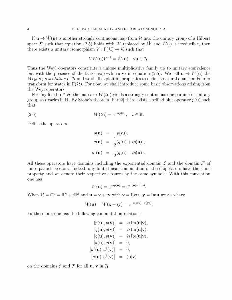
If u→ W (u) is another strongly continuous map from H into the unitary group of a Hilbertspace K such that equation (2.5) holds with W replaced by W and W (·) is irreducible, thenthere exists a unitary isomorphism V : Γ(H)→ K such that

VW (u)V −1 = W (u) ∀u ∈ H.

Thus the Weyl operators constitute a unique multiplicative family up to unitary equivalencebut with the presence of the factor exp−ıIm〈u|v〉 in equation (2.5). We call u → W (u) theWeyl representation ofH and we shall exploit its properties to define a natural quantum Fouriertransform for states in Γ(H). For now, we shall introduce some basic observations arising fromthe Weyl operators.

For any fixed u ∈ H, the map t 7→ W (tu) yields a strongly continuous one parameter unitarygroup as t varies in R. By Stone’s theorem [Par92] there exists a self adjoint operator p(u) suchthat

(2.6) W (tu) = e−ıtp(u), t ∈ R.

Define the operators

q(u) = −p(ıu),

a(u) =1

2(q(u) + ıp(u)),

a†(u) =1

2(q(u)− ıp(u)).

All these operators have domains including the exponential domain E and the domain F offinite particle vectors. Indeed, any finite linear combination of these operators have the sameproperty and we denote their respective closures by the same symbols. With this conventionone has

W (u) = e−ıp(u) = ea†(u)−a(u).

When H = Cn = Rn + ıRn and u = x + ıy with x = Reu, y = Imu we also have

W (u) = W (x + ıy) = e−ı(p(x)−q(y)).

Furthermore, one has the following commutation relations.

[p(u), p(v)] = 2ı Im〈u|v〉,[q(u), q(v)] = 2ı Im〈u|v〉,[q(u), p(v)] = 2ıRe〈u|v〉,[a(u), a(v)] = 0,[a†(u), a†(v)

]= 0,[

a(u), a†(v)]

= 〈u|v〉

on the domains E and F for all u, v in H.

FROM PARTICLE COUNTING TO GAUSSIAN TOMOGRAPHY 5

Choose and fix an orthonormal basis {ej}, j = 1, 2, · · · in H, and define

pj =1√2p(ej), qj = − 1√

2p(ıej),

aj =1√2

(qj + ıpj), a†j =1√2

(qj − ıpj).

Then one has the canonical commutation relations in the form

[pr, ps] = [qr, qs] = 0, [qr, ps] = ıδrs,

or equivalently,

[ar, as] = [a†r, a†s] = 0, [ar, a

†s] = δrs,

in the domains E and F . The observables p1, p2, · · · are called momentum operators andq1, q2, · · · are called position operators in the basis {ej, j = 1, 2, · · · }.

2.3. Quantum Fourier transform. For any trace class operator ρ in Γ(H) its quantumFourier transform or simply Fourier transform ρ on H is defined by

ρ(u) = TrρW (u), u ∈ H.

Then ρ is a bounded continuous function of u satisfying ρ(0) = Trρ. If ρ is positive then ρobeys the Bochner property: for any finite set {cr, r = 1, 2, · · · , k} of scalars and elements{ur, r = 1, 2, · · · , k} in H one has the inequality∑

r,s

crcs exp(ıIm〈ur|us〉)ρ(us − ur) ≥ 0.

Conversely, if ϕ is a continuous function with ϕ(0) = 1 and ϕ satisfies the Bochner propertyabove then there exists a unique state ρ such that ρ = ϕ. When H = Cn one has the Fourierinversion formula:

ρ =1

πn

∫ρ(u)W (u) du

where du denotes integration with respect to the 2n dimensional Lebesgue measure in R2n withdu = dx dy, u = x + ıy, x = Re(u), y = Im(u).

With the help of Fourier transform we shall now construct a natural Hilbert space isomor-phism between the Hilbert space of Hilbert-Schmidt operators in Γ(H) and the Hilbert spaceL2(R2n).

Proposition 2.1. Let H = Cn. Then

1

πn

∫exp

[−‖w‖2 + 〈u|w〉+ 〈w|v〉

]dw = exp〈u|v〉.

Proof. Immediate from standard formulae for Gaussian integrals. �

Proposition 2.2. Denote by L2(H), the Hilbert space of square integrable functions on H withthe scalar product

〈f |g〉 =

∫f(u)g(u)

du

πn

6 K. R. PARTHASARATHY AND RITABRATA SENGUPTA

and by B2(Γ(H)) the Hilbert space of all Hilbert-Schmidt operators on Γ(H) with the scalarproduct

〈ρ1|ρ2〉 = Trρ†1ρ2.

Then there exists a unique Hilbert space isomorphism F : B2(Γ(H))→ L2(H) such that for anyu, v ∈ H,

(2.7) (F(|e(u)〉〈e(v)|)) (w) = Tr|e(u)〉〈e(v)|W (w) ∀w ∈ H.Proof. The right hand side of equation (2.7) is equal to

〈e(v)|W (w)|e(u)〉= e−

12‖w‖2〈e(v)|e−〈w|u〉|e(u + w)〉

= exp

[−1

2‖w‖2 + 〈v|w〉 − 〈w|u〉+ 〈v|u〉

](2.8)

If we put ρj = |e(uj)〉〈e(vj)|, j = 1, 2 then

(2.9) Trρ†1ρ2 = exp [〈u1|u2〉+ 〈v2|v1〉] .On the other hand the scalar product between Tr|e(uj)〉〈e(vj)|W (w), j = 1, 2 reduces byProposition 2.1 and equation (2.8) to the right hand side of (2.9). Now we observe that rankone operators of the form |e(u)〉〈e(v)|, u, v ∈ H constitute a total set in B2(Γ(H)). Thus Fdefined by (2.7) extends uniquely to the whole of B2(Γ(H)). On the other hand functions of wof the form on the right hand side of (2.8) constitute a total set in L2(H). Thus F extends toa Hilbert space isomorphism between B2(Γ(H)) and L2(H). �

2.4. Gaussian state.

Definition 2.1. A state ρ in Γ(H) with H = Cn is called an n-mode Gaussian state if itsFourier transform ρ is given by

(2.10) ρ(x + ıy) = exp

[−ı√

2(lTx−mTy)−(

xy

)TS

(xy

)].

for all x, y ∈ Rn where l, m are elements of Rn and S is a real 2n × 2n symmetric matrixsatisfying the matrix inequality

(2.11) 2S + ı J2n ≥ 0

with

(2.12) J2n =

[0 −InIn 0

],

In being the identity matrix of order n.

Remark 2.1. Equations (2.10)–(2.12) have been written keeping in mind the orders of thecanonical momentum and position observables as p1, p2, · · · , pn, q1, q2, · · · , qn. Sometimes itis more convenient to distinguish the different modes of a Gaussian state by using the orderp1, q1, p2, q2, · · · , pm, qn. This is usually achieved by employing the permutation

σ =

(1 2 3 4 · · · 2n− 1 2n1 n 2 n+ 1 · · · n n+ n

).

FROM PARTICLE COUNTING TO GAUSSIAN TOMOGRAPHY 7

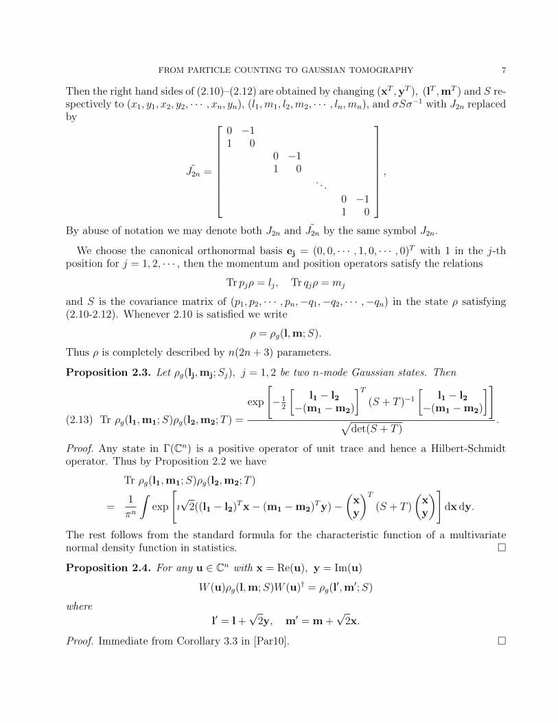
Then the right hand sides of (2.10)–(2.12) are obtained by changing (xT ,yT ), (lT ,mT ) and S re-spectively to (x1, y1, x2, y2, · · · , xn, yn), (l1,m1, l2,m2, · · · , ln,mn), and σSσ−1 with J2n replacedby

J2n =

0 −11 0

0 −11 0

. . .0 −11 0

,

By abuse of notation we may denote both J2n and J2n by the same symbol J2n.

We choose the canonical orthonormal basis ej = (0, 0, · · · , 1, 0, · · · , 0)T with 1 in the j-thposition for j = 1, 2, · · · , then the momentum and position operators satisfy the relations

Tr pjρ = lj, Tr qjρ = mj

and S is the covariance matrix of (p1, p2, · · · , pn,−q1,−q2, · · · ,−qn) in the state ρ satisfying(2.10-2.12). Whenever 2.10 is satisfied we write

ρ = ρg(l,m;S).

Thus ρ is completely described by n(2n+ 3) parameters.

Proposition 2.3. Let ρg(lj,mj;Sj), j = 1, 2 be two n-mode Gaussian states. Then

(2.13) Tr ρg(l1,m1;S)ρg(l2,m2;T ) =

exp

[−1

2

[l1 − l2

−(m1 −m2)

]T(S + T )−1

[l1 − l2

−(m1 −m2)

]]√

det(S + T ).

Proof. Any state in Γ(Cn) is a positive operator of unit trace and hence a Hilbert-Schmidtoperator. Thus by Proposition 2.2 we have

Tr ρg(l1,m1;S)ρg(l2,m2;T )

=1

πn

∫exp

[ı√

2((l1 − l2)Tx− (m1 −m2)Ty)−(

xy

)T(S + T )

(xy

)]dx dy.

The rest follows from the standard formula for the characteristic function of a multivariatenormal density function in statistics. �

Proposition 2.4. For any u ∈ Cn with x = Re(u), y = Im(u)

W (u)ρg(l,m;S)W (u)† = ρg(l′,m′;S)

where

l′ = l +√

2y, m′ = m +√

2x.

Proof. Immediate from Corollary 3.3 in [Par10]. �

8 K. R. PARTHASARATHY AND RITABRATA SENGUPTA

We denote by Sp(2n) the symplectic group Sp(2n,R) of all real 2n×2n matrices L satisfyingthe relation

LTJ2nL = J2n.

Let Γ(L) be the unitary operator in Γ(Cn) which is unique upto a scalar multiple of modulusunity and satisfies the relation

Γ(L)W (x + ıy)Γ(L)−1 = W (x′ + ıy′), ∀x, y ∈ Rn,

where

L

(xy

)=

(x′

y′

).

If U is any n × n unitary matrix and U = A + ı B where A = Re(U) and B = Im(U) thenthe 2n× 2n matrix

L =

[A −BB A

]is an orthogonal matrix which is also an element of Sp(2n). We denote the corresponding Γ(L)by Γ(U) and call it the second quantization of U . We can realize Γ(U) as the unique unitaryoperator satisfying

Γ(U)e(u) = e(Uu) ∀u ∈ Cn.

With these notations we have

Proposition 2.5. For any L ∈ Sp(2n)

Γ(L)ρg(l,m;S)Γ(L)† = ρg(l′,m′;S ′)

where (l′

−m′

)= (L−1)T

(l′

−m′

)S ′ = (L−1)TSL−1.

Proof. This is Corollary 3.5 of [Par10]. �

3. Particle counts and their statistics in a Gaussian state

Let ρg(l,m;S) be an n-mode Gaussian state in Γ(Cn) and whose Fourier transform is givenby equation (2.10). Define the observables

Nj = a†jaj =1

2(p2j + q2j − 1), 1 ≤ j ≤ n.

N =n∑j=1

Nj.

Both Nj and N are observables with spectrum {0, 1, 2, · · · }. Nj is called the number operatoror observable which counts the number of particles (photons) in the j-th mode. Since theNj’s commute with each other they have a joint distribution in the state ρg(l,m;S) withsupport in {0, 1, 2, · · · }n. Using Proposition 2.3 we shall derive a formula for the probabilitygenerating function of this joint distribution and arrive at some natural corollaries. To this endwe introduce the Gaussian state

FROM PARTICLE COUNTING TO GAUSSIAN TOMOGRAPHY 9

ρ(0,0;T ) =n∏j=1

(1− e−tj)e−∑n

j=1 tja†jaj ;

where

T =

12

(1+e−t1

1−e−t1

)I2

. . .12

(1+e−tn

1−e−tn

)I2

= D

(1

2

(1 + e−tj

1− e−tj

)I2, 1 ≤ j ≤ n

); tj > 0 ∀j,

with D indicating the diagonal block matrix with blocks of order 2× 2 and the diagonal entriesbeing enumerated within ( ). These are the well-known thermal states. It follows immediatelyfrom Proposition 2.3, equation(2.13) that

Trρg(l,m;S)e−∑n

j=1 tja†jaj =

exp

[−1

2

(l−m

)T (S +D

(12

(1+e−tj

1−e−tj

)I2, 1 ≤ j ≤ n

))−1( l−m

)]∏n

j=1(1− e−tj)√

det[S +D

(12

(1+e−tj

1−e−tj

)I2, 1 ≤ j ≤ n

)] .

Substituting Nj = a†jaj, xj = e−tj we get(3.1)

Trρg(l,m;S)xN11 · · ·xNn

n =

exp

[−1

2

(l−m

)T (S +D

(12

(1+xj1−xj

)I2, 1 ≤ j ≤ n

))−1( l−m

)]∏n

j=1(1− xj)√

det[S +D

(12

(1+xj1−xj

)I2, 1 ≤ j ≤ n

)]for 0 < xj < 1 ∀j. The right hand side of this equation is nothing but the probability generatingfunction of the joint distribution of the observables Nj, 1 ≤ j ≤ n.

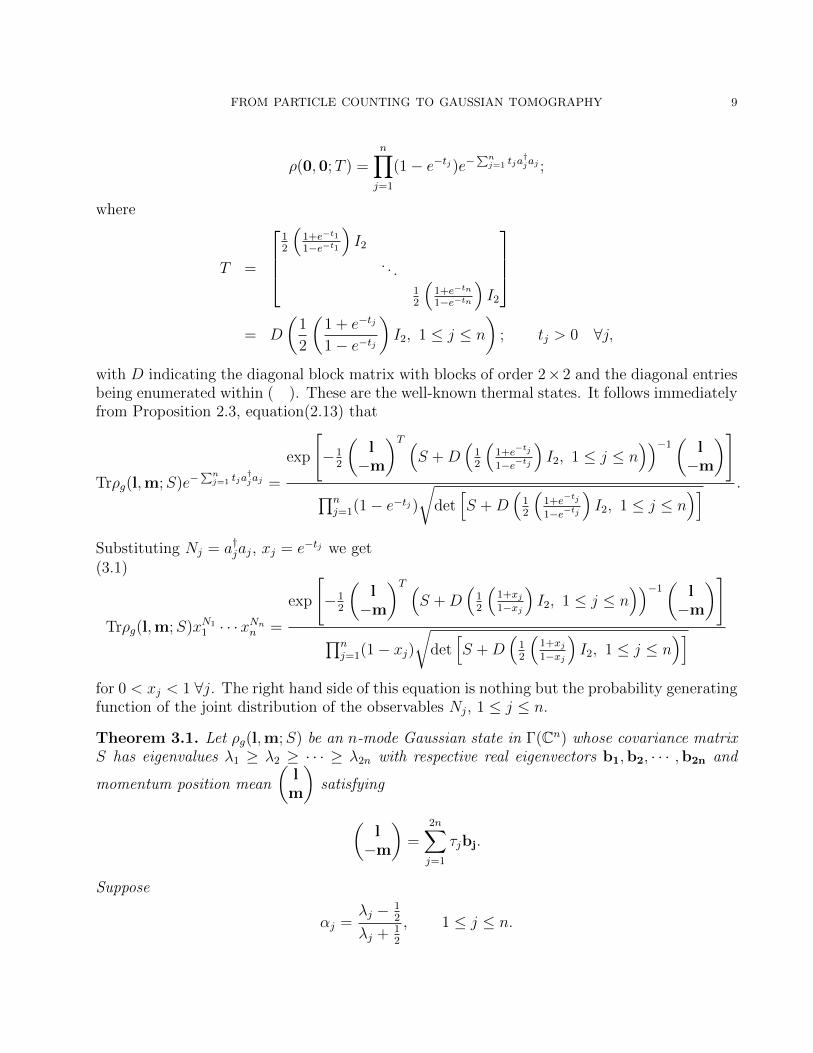
Theorem 3.1. Let ρg(l,m;S) be an n-mode Gaussian state in Γ(Cn) whose covariance matrixS has eigenvalues λ1 ≥ λ2 ≥ · · · ≥ λ2n with respective real eigenvectors b1,b2, · · · ,b2n and

momentum position mean

(l

m

)satisfying

(l−m

)=

2n∑j=1

τjbj.

Suppose

αj =λj − 1

2

λj + 12

, 1 ≤ j ≤ n.

10 K. R. PARTHASARATHY AND RITABRATA SENGUPTA

Then the probability generating function GN(x) of the distribution of the total number operatorN in the state ρg(l,m;S) is given by

GN(x) = Tr ρg(l,m;S)xN

=2n∏j=1

√1− αj

1− αjxexp

[−1

2τ 2j

(1− x)(1− αj)(1− αjx)

], 0 ≤ x < 1.(3.2)

Proof. Putting xj = x for all j in (3.1) and making use of the eigenbasis and eigenvalues of Swe see that (3.1) becomes

GN(x) =2n∏j=1

exp[−1

2τ 2j(λj + 1

21+x1−x

)−1]√(1− x)λj + 1

2(1 + x)

.

The rest is elementary algebra using the definitions of αj in terms of λj for every j. �

Corollary 3.1. The probability distribution of N in the state ρg(l,m;S) satisfies the following:

(i) Pr(N = 0) =2n∏j=1

(1− αj) exp

[−1

2τ 2j (1− αj)

],(3.3)

(ii) 〈N〉 =1

2

[Tr

(S − 1

2

)+

∥∥∥∥( l−m

)∥∥∥∥2],(3.4)

(iii) Variance(N) =1

2Tr

(S − 1

2

)(S +

1

2

)+

(l−m

)TS

(l−m

),(3.5)

Proof. Property (i) follows by putting x = 0 in (3.2). Properties (ii) and (iii) are obtained from(3.2) by taking the logarithm of GN , differentiating twice and taking limx→1

ddx

(logG(x)) and

limx→1d2

d2x(logG(x)). �

Remark 3.1. Equations (3.3)-(3.5) show that the probability of presence of a particle andthe expectation and variance of the total number of particles get enhanced when the Gaussianstate has a nonzero momentum position mean vector. Indeed, the mean and variance of N tendto infinity as the length of the momentum position mean vector increases to infinity. Equations(3.3) and (3.5) indicate the possibility of estimating the mean and covariance parameters ofa Gaussian state by measuring the number operator under different displacements. We shalldiscuss this approach to the tomography of a Gaussian state in great detail in the next section§4.

It may be noted that the parameters αj in Theorem 3.1 satisfy the inequality |αj| < 1 forevery j. If l and m are null-vectors and αj ≥ 0 for every j then GN(x) assumes the form

GN(x) =2n∏j=1

(1− αj

1− αjx

) 12

and the corresponding distribution of N is a convolution of 2n negative binomial distributionsof index 1

2, some of which may be degenerate at 0. In particular, it is infinitely divisible. In

FROM PARTICLE COUNTING TO GAUSSIAN TOMOGRAPHY 11

this case

Variance(N)− 〈N〉 =1

2Tr

(S − 1

2

)2

≥ 0

and the distribution exhibits a super Poissonian property. When S = 12I2n the state becomes

the vacuum state and N has the degenerate distribution, degenerate at 0.Now we shall analyse the distribution of N in a pure Gaussian state. In this case S = 1

2LTL

for some element L of the group Sp(2n) and its eigenvalues can be expressed as

(3.6)

(c12,

1

2c1,c22,

1

2c2, · · · , ck

2,

1

2ck,1

2, · · · , 1

2

)where cj > 1 for 1 ≤ j ≤ k. Then

α2j−1 =cj−1cj+1

> 0 for 1 ≤ j ≤ k,

α2j =1−cj1+cj

< 0 for 1 ≤ j ≤ k,

αr = 0 for 2k + 1 ≤ r ≤ 2n.

Write βj = α2j−1, 1 ≤ j ≤ k so that α2j = −βj, 1 ≤ j ≤ k. Then the probability generatingfunction of the total number operator N in (3.2) assumes the form

(3.7) GN(x) = G1(x)G2(x)G3(x)

where

G1(x) =k∏j=1

√1− β2

j

1− β2jx

2(3.8)

G2(x) = exp1

2

k∑j=1

[τ 22j−1

(x− 1)(1− βj)1− βjx

+ τ 22j(x− 1)(1 + βj)

1 + βjx

](3.9)

G3(x) = exp

[1

2

2n∑j=2k+1

τ 2j (x− 1)

](3.10)

where 0 < βj < 1 for 1 ≤ j ≤ k.Writing

γj = τ 22j−1(1− βj),(3.11)

δj = τ 22j(1 + βj), 1 ≤ j ≤ k,(3.12)

one can express G2(x) in (3.9) as

(3.13) G2(x) = exp1

2

k∑j=1

βj(γj − δj)(x2 − 1) + [γj(1− βj) + δj(1 + βj)] (x− 1)

1− β2jx

2

where 0 < βj < 1, γj ≥ 0, δj ≥ 0 for 1 ≤ j ≤ k.From (3.7) it follows that G1(x) is the probability generating function of a convolution of

probability distributions µj, 1 ≤ j ≤ k where the probability generating function of µj is equal

12 K. R. PARTHASARATHY AND RITABRATA SENGUPTA

to

(1− β2j )

12

∞∑r=0

1.3.5. · · · (2r + 1)

r!β2rj x

2r, 1 ≤ j ≤ k.

In particular µj is an infinitely divisible distribution with support in {0, 2, 4, · · · }. Equation(3.10) shows that G3(x) is the probability generating function of a Poisson distribution withmean value 1

2

∑2nr=2k+1 τ

2r .

If γj ≥ δj for every j = 1, 2, · · · , k then G2(x) is clearly the probability generating function ofan infinitely divisible distribution with support in {0, 1, 2, · · · }. Its Levy measure can be easilyread off from (3.13). Under this assumption, i.e. γj ≥ δj for each 1 ≤ j ≤ k it follows that Nhas an infinitely divisible distribution in the pure Gaussian state we started with.

However, we do not know the answer to the question whether the distribution of the totalnumber operator N in every Gaussian state is infinitely divisible and hence of a mixed Poissontype.

4. From particle counting to the tomography of a Gaussian state

A Gaussian state with n modes can be constructed if its momentum and position means l,m and its covariance matrix S are known. Our aim is to express these parameters in terms ofthe expectation values of conjugates of the total number operator by a few elementary gatesin the Hilbert space Γ(Cn). To this end we shall make use of the Weyl displacement operatorsW (u), u ∈ Cn and the Gaussian symmetries Γ(L), L ∈ Sp(2n) described in Section §3. Westart with an elementary but basic result for achieving this tomography of a Gaussian state.For any observable X denote by 〈X〉 its mean value in the state relevant to the context.

Theorem 4.1. Let ρg(l,m;S) be a Gaussian state and let N be the number operator in then-mode Hilbert space Γ(Cn). Then the following hold:

(i) For all x, y ∈ Rn

(4.1)⟨W (x + ıy)†NW (x + ıy)

⟩− 〈N〉 = ‖x‖2 + ‖y‖2 +

√2(yT l + xTm)

(ii) For any L ∈ Sp(2n)(4.2)⟨

Γ(L)†NΓ(L)⟩− 〈N〉 =

1

2

[TrS

(L−1L−1

T − I2n)

+

(l−m

)T (L−1L−1

T − I2n)(

l−m

)].

Proof. We have from Proposition 2.4 and equation (3.4)⟨W (x + ıy)†NW (x + ıy)

⟩= Tr ρg(l,m;S)W (x + ıy)†NW (x + ıy)

= Tr W (x + ıy)ρg(l,m;S)W (x + ıy)†N

=1

2

[Tr

(S − 1

2

)+ ‖l +

√2y‖2 + ‖m +

√2x‖2

].

Now subtracting the value of 〈N〉 given by (3.4) we obtain equation (4.1).

FROM PARTICLE COUNTING TO GAUSSIAN TOMOGRAPHY 13

Similarly , we have from Proposition 2.5 and equation (3.4)

Tr ρg(l,m;S)Γ(L)†NΓ(L) = Tr Γ(L)ρg(l,m;S)Γ(L)†N

=1

2

[Tr

(L−1

TSL−1 − 1

2

)+

(l−m

)TL−1

TL−1

(l−m

)].

Now, subtracting the value of 〈N〉 given by (3.4) get get (4.2). �

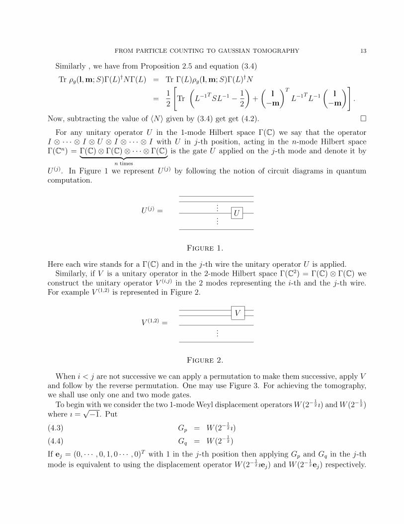
For any unitary operator U in the 1-mode Hilbert space Γ(C) we say that the operatorI ⊗ · · · ⊗ I ⊗ U ⊗ I ⊗ · · · ⊗ I with U in j-th position, acting in the n-mode Hilbert spaceΓ(Cn) = Γ(C)⊗ Γ(C)⊗ · · · ⊗ Γ(C)︸ ︷︷ ︸

n times

is the gate U applied on the j-th mode and denote it by

U (j). In Figure 1 we represent U (j) by following the notion of circuit diagrams in quantumcomputation.

U......

U (j) =

Figure 1.

Here each wire stands for a Γ(C) and in the j-th wire the unitary operator U is applied.Similarly, if V is a unitary operator in the 2-mode Hilbert space Γ(C2) = Γ(C) ⊗ Γ(C) we

construct the unitary operator V (i,j) in the 2 modes representing the i-th and the j-th wire.For example V (1,2) is represented in Figure 2.

V

...

V (1,2) =

Figure 2.

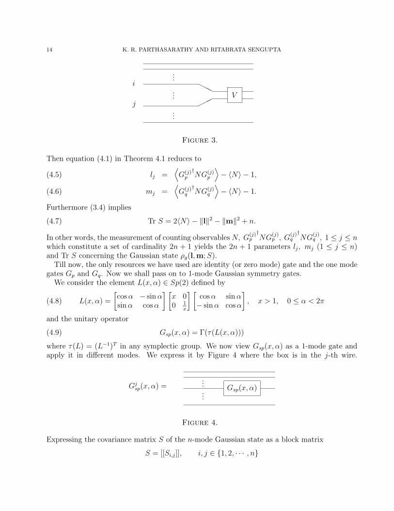
When i < j are not successive we can apply a permutation to make them successive, apply Vand follow by the reverse permutation. One may use Figure 3. For achieving the tomography,we shall use only one and two mode gates.

To begin with we consider the two 1-mode Weyl displacement operators W (2−12 ı) and W (2−

12 )

where ı =√−1. Put

Gp = W (2−12 ı)(4.3)

Gq = W (2−12 )(4.4)

If ej = (0, · · · , 0, 1, 0 · · · , 0)T with 1 in the j-th position then applying Gp and Gq in the j-th

mode is equivalent to using the displacement operator W (2−12 ıej) and W (2−

12 ej) respectively.

14 K. R. PARTHASARATHY AND RITABRATA SENGUPTA

i

j

HHH

���

V

...

...

...

Figure 3.

Then equation (4.1) in Theorem 4.1 reduces to

lj =⟨G(j)p

†NG(j)

p

⟩− 〈N〉 − 1,(4.5)

mj =⟨G(j)q

†NG(j)

q

⟩− 〈N〉 − 1.(4.6)

Furthermore (3.4) implies

(4.7) Tr S = 2〈N〉 − ‖l‖2 − ‖m‖2 + n.

In other words, the measurement of counting observables N, G(j)p

†NG

(j)p , G

(j)q

†NG

(j)q , 1 ≤ j ≤ n

which constitute a set of cardinality 2n + 1 yields the 2n + 1 parameters lj, mj (1 ≤ j ≤ n)and Tr S concerning the Gaussian state ρg(l,m;S).

Till now, the only resources we have used are identity (or zero mode) gate and the one modegates Gp and Gq. Now we shall pass on to 1-mode Gaussian symmetry gates.

We consider the element L(x, α) ∈ Sp(2) defined by

(4.8) L(x, α) =

[cosα − sinαsinα cosα

] [x 00 1

x

] [cosα sinα− sinα cosα

], x > 1, 0 ≤ α < 2π

and the unitary operator

(4.9) Gsp(x, α) = Γ(τ(L(x, α)))

where τ(L) = (L−1)T in any symplectic group. We now view Gsp(x, α) as a 1-mode gate andapply it in different modes. We express it by Figure 4 where the box is in the j-th wire.

Gsp(x, α)......

Gjsp(x, α) =

Figure 4.

Expressing the covariance matrix S of the n-mode Gaussian state as a block matrix

S = [[Si,j]], i, j ∈ {1, 2, · · · , n}

FROM PARTICLE COUNTING TO GAUSSIAN TOMOGRAPHY 15

where each Si,j is a 2×2 matrix we observe that Sjj is the covariance matrix of the j-th marginalGaussian state and

(4.10)

[Sii SijSTij Sjj

], i < j

is the covariance matrix of the i j-marginal Gaussian state of ρg(l,m;S).Let

(4.11) Sjj =

[σpp σpqσqp σqq

]with σqp = σpq. Thus Sjj has three parameters. Applying the gate G

(j)sp (x, α) defined by (4.9)

and Figure 4, and using part (ii) of Theorem 4.1 we get

(4.12)

(x2 cos2 α + x−2 sin2 α− 1)σpp + (x2 sin2 α + x−2 cos2 α− 1)σqq + 2(x2 − x−2) sinα cosα

= 2(⟨G(j)sp (x, α)†NG(j)

sp (x, α)⟩− 〈N〉

)+ [1− (x2 cos2 α + x−2 sin2 α)]l2j

+ [1− (x2 sin2 α + x−2 cos2 α)]m2j + 2ljmj(x

2 − x−2) sinα cosα

Choosing α = 0, (4.12) becomes

(x2 − 1)σpp + (x−2 − 1)σqq

= 2(⟨G(j)sp (x, 0)†NG(j)

sp (x, 0)⟩− 〈N〉

)+ (1− x2)l2j + (1− x−2)m2

j .(4.13)

Choosing x =√

2 and x =√

3 successively (4.13) yields two linearly independent equations for

determining σpp and σqq in terms of lj, mj, 〈N〉 and⟨G

(j)sp (x, 0)†NG

(j)sp (x, 0)

⟩.

Now we go back to the equation (4.12) and choose x =√

2, α = π4. Then we get

1

4(σpp + σqq) +

3

2σpq = 2

(⟨G(j)sp

(√2,π

4

)†NG(j)

sp

(√2,π

4

)⟩− 〈N〉

)−1

4(l2j +m2

j) +3

2ljmj.(4.14)

Since σpp, σqq and lj, mj have already been determined, (4.14) determines σpq by using values

of 〈N〉 and⟨G

(j)sp

(√2, π

4

)†NG

(j)sp

(√2, π

4

)⟩. Thus Sjj can be completely determined by mea-

surements of N using the gates Gsp(√

2, 0), Gsp(√

3, 0) and Gsp(√

2, π4) in different modes after

knowing the vectors l and m. However, after determining Sjj for 1 ≤ j ≤ n − 1, in order to

determine Snn it is enough to use only the two gates Gsp(√

2, 0) and Gsp(√

2, π4) in the n-th

mode because we already know TrS form (4.7). Thus we need only (3n−1) new measurementsto determine the 3n parameters occurring in the block diagonals Sjj, 1 ≤ j ≤ n.

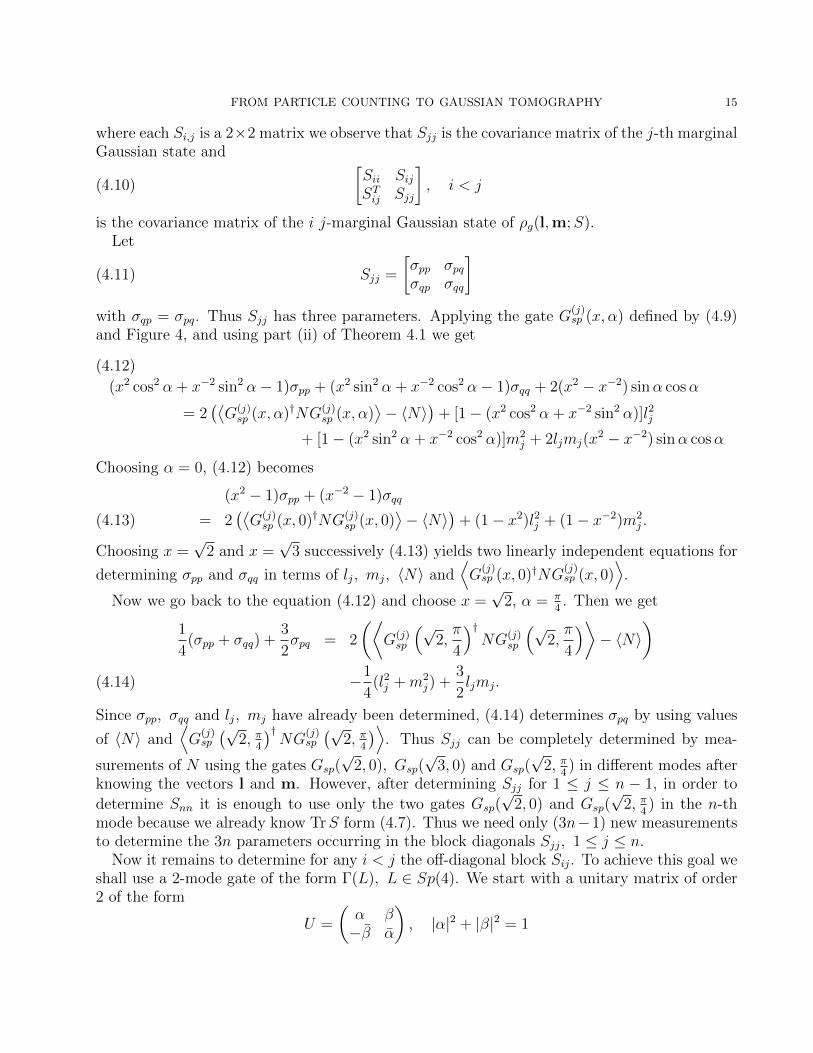
Now it remains to determine for any i < j the off-diagonal block Sij. To achieve this goal weshall use a 2-mode gate of the form Γ(L), L ∈ Sp(4). We start with a unitary matrix of order2 of the form

U =

(α β−β α

), |α|2 + |β|2 = 1

16 K. R. PARTHASARATHY AND RITABRATA SENGUPTA

where α = α1 + ı α2, β = β1 + ı β2 with αj, βj being real. If we view U as a real lineartransformation of R4 we get an element of Sp(4) of the form

(4.15) O =

α1 −α2 β1 −β2α2 α1 β2 β1−β1 −β2 α1 α2

β2 −β1 −α2 α1

where O is a real orthogonal matrix. Define

(4.16) L(U, x1, x2) = O

x1

x−11

x2x−12

OT , x1 > 1, x2 > 1.

We write

(4.17) L(U, x1, x2)TL(U, x1, x2) =

[A BT

B C

]and note that A, C are 2× 2 positive definite matrices and B is given by

(4.18) B =

[−β1α1(x1 − x2) + β2α2(x

−11 − x−12 ) −β1α2(x1 − x−12 )− β2α1(x

−11 − x2)

β2α1(x1 − x−12 ) + β1α2(x−11 − x2) β2α2(x1 − x2)− β1α1(x

−11 − x−12 )

].

Using (4.10) and (4.17) we observe that

Tr

[Sii SijSji Sjj

]L(U, x1, x2)

TL(U, x1, x2) = Tr

[Sii SijSji Sjj

] [A BT

B C

]= Tr(SiiA+ SjjC) + 2TrSijB(4.19)

where the first sum on the right hand side depends only on Sii and Sjj which have already beendetermined in terms of the expectations of N and its conjugates by chosen one mode gates. Inorder to determine Sij we use the 2-mode gate

(4.20) Gsp(U, x1, x2) = Γ(τ(L(U, x1, x2)))

in the (i, j)-modes and use part (ii) of Theorem 4.1 to obtain the relation

⟨Gi,jsp (U, x1, x2)

†NGi,jsp (U, x1, x2)

⟩− 〈N〉

=1

2

Tr

[Sii SijSji Sjj

] [A− I2 BT

B C − I2

]+

l1−m1

l2−m2

T [A− I2 BT

B C − I2

]l1−m1

l2−m2

.

Using (4.19) this reduces to

Tr SijB =⟨Gi,jsp (U, x1, x2)

†NGi,jsp (U, x1, x2)

⟩− 〈N〉

−1

2Tr [Sii(A− I2) + Sjj(C − I2)]

= f(U, x1, x2) say.(4.21)

FROM PARTICLE COUNTING TO GAUSSIAN TOMOGRAPHY 17

When li, mi, lj, mj, Sii and Sjj are already determined, the term f(U, x1, x2) depends onlyon U, x1, x2. Let

Sij =

[γ11 γ12γ21 γ22

].

We now make four special cases for (U, x1, x2).

(i) U = H = 1√2

[1 1−1 1

], x1 = 1, x2 = 2. Put r1 = f(H, 1, 2). Then (4.21) becomes

(4.22)1

2γ11 −

1

4γ22 = r1.

(ii) U = H, x1 = 1, x2 = 3. Put r2 = f(H, 1, 3). Then (4.21) becomes

(4.23) γ11 −1

3γ22 = r2.

(iii) U = K = 1√2

[ı 1−1 −ı

], x1 = 1, x2 = 2. Put r3 = f(K, 1, 2). Then (4.21) becomes

(4.24) − 1

4(γ21 + 2γ12) = r3.

(iv) U = K, x1 = 1, x2 = 3. Put r4 = f(K, 1, 3). Then (4.21) becomes

(4.25) − 1

3(γ21 + 3γ12) = r4.

The four equations (4.22)–(4.25) in the unknowns γ11, γ22, γ12, γ21 are linear and linearlyindependent. Thus they determine the matrix Sij for any fixed i, j. For this purpose we haveused exactly four measurements described by the four 2-mode gates for four parameters.

In all we have used exactly (2n + 1) + (3n − 1) + 4n(n−1)2

= n(2n + 3) measurements todetermine the n(2n+ 3) parameters of the Gaussian state ρg(l,m;S).

5. Tomography of Gaussian channels

An n-mode Gaussian channel K(A,B) is described by a pair of real 2n× 2n matrices (A,B)where B is positive semidefinite and the following matrix inequality holds:

B + ı(ATJ2nA− J2n) ≥ 0

with J2n as in equation (2.12). Thus K(A,B) is determined by 6n2 + n real parameters. Sucha channel has the property that for any Gaussian input state ρg(l,m;S), the correspondingoutput is again Gaussian and has the form ρg(l

′,m′;S ′) where(l′

−m′

)= AT

(l−m

)(5.1)

S ′ = ATSA+1

2B.(5.2)

18 K. R. PARTHASARATHY AND RITABRATA SENGUPTA

our aim is to determine A and B by performing tomography on the output states for a smallnumber of coherent input statea |ψ(u)〉 where

|ψ(u)〉〈ψ(u)| = ρg

(√2y,√

2x;1

2I2n

)where x = Re(u), y = Im(u). By (5.1) and (5.2) the output state is

(5.3) ρg

(y′,x′;

1

2(ATA+B)

)where

(5.4)

(y′

−x′

)= AT

( √2y

−√

2x

).

Now we specialize the values of u and select the 2n input states

ρj = |ψ(2−12 ıej)〉〈ψ(2−

12 ıej)|, 1 ≤ j ≤ n,(5.5)

ρ′j = |ψ(2−12 ej)〉〈ψ(2−

12 ej)|, 1 ≤ j ≤ n.(5.6)

Then the corresponding output states are

(5.7) ρg

(lj, mj,

1

2(ATA+B)

)with

(5.8)

(lj−mj

)= AT

(ej

0

), 1 ≤ j ≤ n

and

(5.9) ρg′(

lj′, mj

′,1

2(ATA+B)

)with

(5.10)

(lj′

−mj′

)= AT

(0ej

), 1 ≤ j ≤ n.

A full tomography on (5.7) with j = 1 as outlined in Section §4 yields the first row of A andthe matrix ATA+B by using n(2n+3) measurements. A similar but partial tomography of theremaining (n− 1) states in (5.7) and all the states in (5.9) but only for the mean values yieldsthe remaining (2n− 1) rows of A. This needs an additional set of (2n− 1)(2n + 1) = 4n2 − 1measurements. In all, our approach requires 6n2 + 3n− 1 measurements for getting the 6n2 +nparameters. It will be interesting to know whether one can determine A and B with lessmeasurements. If this is not possible our problem will carry an intrinsic tomographic complexity.

FROM PARTICLE COUNTING TO GAUSSIAN TOMOGRAPHY 19

6. Conclusions

All the 2n2 + 3n mean and covariance parameters of an n-mode Gaussian state can be recov-ered from the expectation values of the same number of conjugates of the total number operatorby Gaussian symmetries. Such symmetries can be realised by five one mode and four two modegates. The complete tomography of a Gaussian state can be expressed by circuit diagrams andmeasurements akin to those in quantum computation theory. An application of this tomogra-phy to the output of an n-mode Gaussian channel corresponding to appropriate coherent inputsdetermines all the 6n2 + n parameters by 6n2 + 3n − 1 measurements. Improvement in thischannel tomography and finding the probability distribution of the number operator from itsexplicitly computable probability generating function in a general n-mode Gaussian state seemto be interesting problems arising from our investigations.

References

[ADMS95] Arvind, B Dutta, N Mukunda, and R Simon. The real symplectic groups in quantum mechanicsand optics. Pramana, 45:471–497, 1995.

[dG06] Maurice de Gosson. Symplectic geometry and quantum mechanics, volume 166 of Operator The-ory: Advances and Applications. Birkhauser Verlag, Basel, 2006. Advances in Partial DifferentialEquations (Basel).

[HHW10] Teiko Heinosaari, Alexander S. Holevo, and Michael M. Wolf. The semigroup structure of Gaussianchannels. Quantum Inf. Comput., 10(7-8):619–635, 2010.

[Hol12] Alexander S. Holevo. Quantum systems, channels, information. A mathematical introduction.Berlin: de Gruyter, 2012.

[LKK+08] Mirko Lobino, Dmitry Korystov, Connor Kupchak, Eden Figueroa, Barry C. Sanders, and A. I.Lvovsky. Complete characterization of quantum-optical processes. Science, 322(5901):563–566,2008.

[LR09] A. I. Lvovsky and M. G. Raymer. Continuous-variable optical quantum-state tomography. Rev.Mod. Phys., 81:299–332, Mar 2009.

[Par92] K. R. Parthasarathy. An introduction to quantum stochastic calculus, volume 85 of Monographs inMathematics. Birkhauser Verlag, Basel, 1992.

[Par10] K. R. Parthasarathy. What is a Gaussian state? Commun. Stoch. Anal., 4(2):143–160, 2010.[Par13] Kalyanapuram R. Parthasarathy. The symmetry group of Gaussian states in L2(Rn). In Albert N.

Shiryaev, S. R. S. Varadhan, and Ernst L. Presman, editors, Prokhorov and contemporary prob-ability theory. In honor of Yuri V. Prokhorov on the occasion of his 80th birthday, volume 33 ofSpringer Proceedings in Mathematics & Statistics, pages 349–369. Berlin: Springer, 2013.

[Par14a] K. R. Parthasarathy. Quantum Stochastic Calculus and Quantum Gaussian Processes. ArXiv e-prints, Aug 2014, 1408.5686.

[Par14b] K. R. Parthasarathy. Symplectic Dilations, Gaussian States and Gaussian Channels. ArXiv e-prints, May 2014, 1405.6476.

[PR04] Matteo Paris and Jaroslav Rehacek, editors. Quantum state estimation, volume 649 of LectureNotes in Physics. Springer-Verlag, Berlin, 2004.

[RKSM+11] Saleh Rahimi-Keshari, Artur Scherer, Ady Mann, A T Rezakhani, A I Lvovsky, andBarry C Sanders. Quantum process tomography with coherent states. New Journal of Physics,13(1):013006, 2011.

[SW87a] W. Schleich and J. A. Wheeler. Oscillations in photon distribution of squeezed states. J. Opt. Soc.Am. B, 4(10):1715–1722, Oct 1987.

[SW87b] W. Schleich and J. A. Wheeler. Oscillations in photon distribution of squeezed states and inter-ference in phase space. Nature, 326(6113):574–577, Apr 1987.

20 K. R. PARTHASARATHY AND RITABRATA SENGUPTA

[WPGP+12] Christian Weedbrook, Stefano Pirandola, Raul Garcıa-Patron, Nicolas J. Cerf, Timothy C. Ralph,Jeffrey H. Shapiro, and Seth Lloyd. Gaussian quantum information. Rev. Mod. Phys., 84:621–669,May 2012.

[WYH+13] Xiang-Bin Wang, Zong-Wen Yu, Jia-Zhong Hu, Adam Miranowicz, and Franco Nori. Efficienttomography of quantum-optical gaussian processes probed with a few coherent states. Phys. Rev.A, 88:022101, Aug 2013.

Theoretical Statistics and Mathematics Unit, Indian Statistical Institute, Delhi Centre, 7S J S Sansanwal Marg, New Delhi 110 016, India

E-mail address, K R Parthasarathy: krp@isid.ac.in

Theoretical Statistics and Mathematics Unit, Indian Statistical Institute, Delhi Centre, 7S J S Sansanwal Marg, New Delhi 110 016, India

E-mail address, Ritabrata Sengupta: rb@isid.ac.in