Rounding error and conditioning, Gaussian elimination, LU ...

Production of this 2015 edition, containing corrections and minor revisions of the 2008 edition, was funded by the sigma Network.

About the HELM Project HELM (Helping Engineers Learn Mathematics) materials were the outcome of a three-‐year curriculum development project undertaken by a consortium of five English universities led by Loughborough University, funded by the Higher Education Funding Council for England under the Fund for the Development of Teaching and Learning for the period October 2002 – September 2005, with additional transferability funding October 2005 – September 2006. HELM aims to enhance the mathematical education of engineering undergraduates through flexible learning resources, mainly these Workbooks. HELM learning resources were produced primarily by teams of writers at six universities: Hull, Loughborough, Manchester, Newcastle, Reading, Sunderland. HELM gratefully acknowledges the valuable support of colleagues at the following universities and colleges involved in the critical reading, trialling, enhancement and revision of the learning materials: Aston, Bournemouth & Poole College, Cambridge, City, Glamorgan, Glasgow, Glasgow Caledonian, Glenrothes Institute of Applied Technology, Harper Adams, Hertfordshire, Leicester, Liverpool, London Metropolitan, Moray College, Northumbria, Nottingham, Nottingham Trent, Oxford Brookes, Plymouth, Portsmouth, Queens Belfast, Robert Gordon, Royal Forest of Dean College, Salford, Sligo Institute of Technology, Southampton, Southampton Institute, Surrey, Teesside, Ulster, University of Wales Institute Cardiff, West Kingsway College (London), West Notts College.

HELM Contacts: Post: HELM, Mathematics Education Centre, Loughborough University, Loughborough, LE11 3TU. Email: [email protected] Web: http://helm.lboro.ac.uk

HELM Workbooks List 1 Basic Algebra 26 Functions of a Complex Variable 2 Basic Functions 27 Multiple Integration 3 Equations, Inequalities & Partial Fractions 28 Differential Vector Calculus 4 Trigonometry 29 Integral Vector Calculus 5 Functions and Modelling 30 Introduction to Numerical Methods 6 Exponential and Logarithmic Functions 31 Numerical Methods of Approximation 7 Matrices 32 Numerical Initial Value Problems 8 Matrix Solution of Equations 33 Numerical Boundary Value Problems 9 Vectors 34 Modelling Motion 10 Complex Numbers 35 Sets and Probability 11 Differentiation 36 Descriptive Statistics 12 Applications of Differentiation 37 Discrete Probability Distributions 13 Integration 38 Continuous Probability Distributions 14 Applications of Integration 1 39 The Normal Distribution 15 Applications of Integration 2 40 Sampling Distributions and Estimation 16 Sequences and Series 41 Hypothesis Testing 17 Conics and Polar Coordinates 42 Goodness of Fit and Contingency Tables 18 Functions of Several Variables 43 Regression and Correlation 19 Differential Equations 44 Analysis of Variance 20 Laplace Transforms 45 Non-‐parametric Statistics 21 z-‐Transforms 46 Reliability and Quality Control 22 Eigenvalues and Eigenvectors 47 Mathematics and Physics Miscellany 23 Fourier Series 48 Engineering Case Study 24 Fourier Transforms 49 Student’s Guide 25 Partial Differential Equations 50 Tutor’s Guide

© Copyright Loughborough University, 2015

ContentsContents 3030

Numerical Methods

Introduction to

30.1 Rounding Error and Conditioning 2

30.2 Gaussian Elimination 12

30.3 LU Decomposition 21

30.4 Matrix Norms 34

30.5 Iterative Methods for Systems of Equations 46

Learning

In this Workbook you will learn about some of the issues involved with usinga computer to carry out numerical calculations for engineering problems. For example, the effect of rounding error will be discussed.

Most of this Workbook will consider methods for solving systems of equations.In particular you will see how methods can be adapted so that rounding errorbecomes less of a problem.

outcomes

Rounding Error andConditioning

��

��30.1

IntroductionIn this first Section concerning numerical methods we will discuss some of the issues involved withdoing arithmetic on a computer. This is an important aspect of engineering. Numbers cannot,in general, be represented exactly, they are typically stored to a certain number of significantfigures. The associated rounding error and its accumulation are important issues which need tobe appreciated if we are to trust computational output.

We will also look at ill-conditioned problems which can have an unfortunate effect on rounding error.

�

�

�

�Prerequisites

Before starting this Section you should . . .

• recall the formula for solving quadraticequations

'

&

$

%

Learning OutcomesOn completion you should be able to . . .

• round real numbers and know what theassociated rounding error is

• understand how rounding error can grow incalculations

• explain what constitutes an ill-conditionedproblem

2 HELM (2015):Workbook 30: Introduction to Numerical Methods

®

1. Numerical methodsMany mathematical problems which arise in the modelling of engineering situations are too difficult,or too lengthy, to tackle by hand. Instead it is often good enough to resort to an approximation givenby a computer. Indeed, the process of modelling a “real world” situation with a piece of mathematicswill involve some approximation, so it may make things no worse to seek an approximate solution ofthe theoretical problem.

Evidently there are certain issues here. Computers do not know what a function is, or a vector,or an integral, or a polynomial. Loosely speaking, all computers can do is remember long lists ofnumbers and then process them (very quickly!). Mathematical concepts must be posed as somethingnumerical if a computer is to be given a chance to help. For this reason a topic known as numericalanalysis has grown in recent decades which is devoted to the study of how to get a machine to addressa mathematical problem.

Key Point 1

“Numerical methods” are methods devised to solve mathematical problems on a computer.

2. RoundingIn general, a computer is unable to store every decimal place of a real number. Real numbers arerounded. To round a number to n significant figures we look at the (n + 1)th digit in the decimalexpansion of the number.

• If the (n + 1)th digit is 0, 1, 2, 3 or 4 then we round down: that is, we simply chop to nplaces. (In other words we neglect the (n+ 1)th digit and any digits to its right.)

• If the (n + 1)th digit is 5, 6, 7, 8 or 9 then we round up: we add 1 to the nth decimal placeand then chop to n places.

For example

1

3= 0.3333 rounded to 4 significant figures,

8

3= 2.66667 rounded to 6 significant figures,

π = 3.142 rounded to 4 significant figures.

An alternative way of stating the above is as follows

HELM (2015):Section 30.1: Rounding Error and Conditioning

3

1

3= 0.3333 rounded to 4 decimal places,

8

3= 2.66667 rounded to 5 decimal places,

π = 3.142 rounded to 3 decimal places.

Sometimes the phrases “significant figures” and “decimal places” are abbreviated as “s.f.” or“sig. fig.” and “d.p.” respectively.

Example 1Write down each of these numbers rounding them to 4 decimal places:0.12345, −0.44444, 0.5555555, 0.000127351, 0.000005

Solution

0.1235, −0.4444, 0.5556, 0.0001, 0.0000

Example 2Write down each of these numbers, rounding them to 4 significant figures:0.12345, −0.44444, 0.5555555, 0.000127351, 25679

Solution

0.1235, −0.4444, 0.5556, 0.0001274, 25680

TaskWrite down each of these numbers, rounding them to 3 decimal places:0.87264, 0.1543, 0.889412, −0.5555

Your solution

Answer

0.873, 0.154, 0.889, −0.556


®

Rounding errorClearly, rounding a number introduces an error. Suppose we know that some quantity x is such that

x = 0.762143 6 d.p.

Based on what we know about the rounding process we can deduce that

x = 0.762143 ± 0.5× 10−6.

This is typical of what can occur when dealing with numerical methods. We do not know whatvalue x takes, but we have an error bound describing the furthest x can be from the stated value0.762143. Error bounds are necessarily pessimistic. It is very likely that x is closer to 0.762143 than0.5 × 10−6, but we cannot assume this, we have to assume the worst case if we are to be certainthat the error bound is safe.

Key Point 2

Rounding a number to n decimal places introduces an error that is no larger (in magnitude) than

1

2× 10−n

Note that successive rounding can increase the associated rounding error, for example

12.3456 = 12.3 (1 d.p.),

12.3456 = 12.346 (3 d.p.) = 12.35 (2 d.p.) = 12.4 (1 d.p.).

Accumulated rounding errorRounding error can sometimes grow as calculations progress. Consider these examples.

Example 3Let x =

22

7and y = π. It follows that, to 9 decimal places

x = 3.142857143

y = 3.141592654

x+ y = 6.284449797

x− y = 0.001264489

(i) Round x and y to 7 significant figures. Find x+ y and x− y.

(ii) Round x and y to 3 significant figures. Find x+ y and x− y.


5

Solution

(i) To 7 significant figures x = 3.142857 and y = 3.141593 and it follows that, with this roundingof the numbers

x+ y = 6.284450

x− y = 0.001264.

The outputs (x + y and x − y) are as accurate to as many decimal places as the inputs (xand y). Notice however that the difference x− y is now only accurate to 4 significant figures.

(ii) To 3 significant figures x = 3.14 and y = 3.14 and it follows that, with this rounding of thenumbers

x+ y = 6.28

x− y = 0.

This time we have no significant figures accurate in x− y.

In Example 3 there was loss of accuracy in calculating x−y. This shows how rounding error can growwith even simple arithmetic operations. We need to be careful when developing numerical methodsthat rounding error does not grow. What follows is another case when there can be a loss of accuratesignificant figures.

TaskThis Task involves solving the quadratic equation

x2 + 30x+ 1 = 0

(a) Use the quadratic formula to show that the two solutions of x2+30x+1 = 0are x = −15±

√224.

(b) Write down the two solutions to as many decimal places as your calculatorwill allow.

(c) Now round√224 to 4 significant figures and recalculate the two solutions.

(d) How many accurate significant figures are there in the solutions you obtainedwith the rounded approximation to

√224?


®

Your solution

Answer

(a) From the quadratic formula x =−30±

√302 − 4

2= −15 ±

√152 − 1 = −15 ±

√224 as

required.

(b) −15 +√224 = −0.03337045291 is one solution and −15 −

√224 = −29.96662955 is the

other, to 10 significant figures.

(c) Rounding√224 to 4 significant figures gives

−15 +√224 = −15 + 14.97 = −0.03 − 15−

√224 = −15− 14.97 = −29.97

(d) The first of these is only accurate to 1 sig. fig., the second is accurate to 4 sig. fig.

TaskIn the previous Task it was found that rounding to 4 sig. fig. led to a result witha large error for the smaller root of the quadratic equation. Use the fact that forthe general quadratic

ax2 + bx+ c = 0

the product of the two roots isc

ato determine the smaller root with improved

accuracy.

Your solution


7

Answer

Here a = 1, b = 30, c = 1 so the product of the roots =c

a= 1. So starting from the rounded

value −29.97 for the larger root we obtain the smaller root to be1

−29.97≈ −0.03337 with 4 sig.

fig. accuracy.

(This indirect method is often built into computer software to increase accuracy.)

3. Well-conditioned and ill-conditioned problemsSuppose we have a mathematical problem that depends on some input data. Now imagine alteringthe input data by a tiny amount. If the corresponding solution always varies by a correspondinglytiny amount then we say that the problem is well-conditioned. If a tiny change in the input resultsin a large change in the output we say that the problem is ill-conditioned. The following Exampleshould help.

Example 4Show that the evaluation of the function f(x) = x2 − x− 1500 near x = 39is an ill-conditioned problem.

Solution

Consider f(39) = −18 and f(39.1) = −10.29. In changing x from 39 to 39.1 we have alteredit by about 0.25%. But the percentage change in f is greater than 40%. The demonstrates theill-conditioned nature of the problem.

TaskWork out the derivative

df

dxfor the function used in Example 4 and so explain why

the numerical results show the calculation of f to be ill-conditioned near x = 39.

Your solution


®

Answer

We have f = x2−x−1500 anddf

dx= 2x−1. At x = 39 the value of f is −18 and, using calculus,

the value ofdf

dxis 77. Thus x = 39 is very close to a zero of f (i.e. a root of the quadratic equation

f(x) = 0). The fractional change in f is thus very large even for a small change in x. The givenvalues of f(38.6) and f(39.4) lead us to an estimate of

12.96− (−48.64)39.4− 38.6

fordf

dx. This ratio gives the value 77.0, which agrees exactly with our result from the calculus. Note,

however, that an exact result of this kind is not usually obtained; it is due to the simple quadraticform of f for this example.

One reason that this matters is because of rounding error. Suppose that, in the Example above, weknow is that x is equal to 39 to 2 significant figures. Then we have no chance at all of evaluating fwith confidence, for consider these values

f(38.6) = −48.64f(39) = −18

f(39.4) = 12.96.

All of the arguments on the left-hand sides are equal to 39 to 2 significant figures so all the valueson the right-hand sides are contenders for f(x). The ill-conditioned nature of the problem leaves uswith some serious doubts concerning the value of f .

It is enough for the time being to be aware that ill-conditioned problems exist. We will discuss thissort of thing again, and how to combat it in a particular case, in a later Section of this Workbook.


9

Exercises

1. Round each of these numbers to the number of places or figures indicated

(a) 23.56712 (to 2 decimal places).

(b) −15432.1 (to 3 significant figures).

2. Suppose we wish to calculate

√x+ 1−

√x,

for relatively large values of x. The following table gives values of y for a range of x-values

x√x+ 1−

√x

100 0.049875621120891000 0.0158074374289610000 0.00499987500625100000 0.00158113487726

(a) For each x shown in the table, and working to 6 significant figures evaluate√x+ 1 and

then√x. Find

√x+ 1−

√x by taking the difference of your two rounded numbers. Are

your answers accurate to 6 significant figures?

(b) For each x shown in the table, and working to 4 significant figures evaluate√x+ 1 and

then√x. Find

√x+ 1−

√x by taking the difference of your two rounded numbers. Are

your answers accurate to 4 significant figures?

3. The larger solution of the quadratic equation

x2 + 168x+ 1 = 0

is −84 +√7055 which is equal to −0.0059525919 to 10 decimal places. Round the value√

7055 to 4 significant figures and then use this rounded value to calculate the larger solutionof the quadratic equation. How many accurate significant figures does your answer have?

4. Consider the function

f(x) = x2 + x− 1975

and suppose we want to evaluate it for some x.

(a) Let x = 20. Evaluate f(x) and then evaluate f again having altered x by just 1%.What is the percentage change in f? Is the problem of evaluating f(x), for x = 20, awell-conditioned one?

(b) Let x = 44. Evaluate f(x) and then evaluate f again having altered x by just 1%.What is the percentage change in f? Is the problem of evaluating f(x), for x = 44, awell-conditioned one?

(Answer: the problem in part (a) is well-conditioned, the problem in part (b) is ill-conditioned.)


®

Answers

1. 23.57, −15400.

2. The answers are tabulated below. The 2nd and 3rd columns give values for√x+ 1 and

√x

respectively, rounded to 10 decimal places. The 4th column shows the values of√x+ 1−

√x

also to 10 decimal places. Column (a) deals with part (a) of the question and finds thedifference after rounding the numbers in the 2nd and 3rd columns to 6 significant figures.Column (b) deals with part (b) of the question and finds the difference after rounding thenumbers in the 2nd and 3rd columns to 4 significant figures.

x√x+ 1

√x (a) (b)

100 10.0498756211 10.0000000000 0.0498756211 0.0499 0.05001000 31.6385840391 31.6227766017 0.0158074374 0.0158 0.020010000 100.0049998750 100.0000000000 0.0049998750 0.0050 0.0000100000 316.2293471517 316.2277660168 0.0015811349 0.0010 0.0000

Clearly the answers in columns (a) and (b) are not accurate to 6 and 4 figures respectively.Indeed the last two figures in column (b) are accurate to no figures at all!

3.√7055 = 83.99 to 4 significant figures. Using this value to find the larger solution of the

quadratic equation gives

−84 + 83.99 = −0.01 .

The number of accurate significant figures is 0 because the accurate answer is 0.006 and ‘1′

is not the leading digit (it is ‘6′).

4. (a) f(20) = −1555 and f(20.2) = −1546.76 so the percentage change in f on changingx = 20 by 1% is

−1555− (−1546.76)−1555

× 100% = 0.53%

to 2 decimal places.

(b) f(44) = 5 and f(44.44) = 44.3536 so the percentage change in f on changing x = 44by 1% is

5− 44.3536

5× 100% = −787.07%


Clearly then, the evaluation of f(20) is well-conditioned and that of f(44) is ill-conditioned.


11

Gaussian Elimination��

��30.2

IntroductionIn this Section we will reconsider the Gaussian elimination approach discussed in 8, and wewill see how rounding error can grow if we are not careful in our implementation of the approach. Amethod called partial pivoting, which helps stop rounding error from growing, will be introduced.

'

&

$

%Prerequisites


• revise matrices, especially matrix solution ofequations

• recall Gaussian elimination

• be able to find the inverse of a 2× 2 matrix�

�

�

�Learning Outcomes

On completion you should be able to . . .

• carry out Gaussian elimination withpartial pivoting


®

1. Gaussian eliminationRecall from 8 that the basic idea with Gaussian (or Gauss) elimination is to replace the matrix ofcoefficients with a matrix that is easier to deal with. Usually the nicer matrix is of upper triangularform which allows us to find the solution by back substitution. For example, suppose we have

x1 + 3x2 − 5x3 = 2

3x1 + 11x2 − 9x3 = 4

−x1 + x2 + 6x3 = 5

which we can abbreviate using an augmented matrix to 1 3 −5 23 11 −9 4−1 1 6 5

.

We use the boxed element to eliminate any non-zeros below it. This involves the following rowoperations 1 3 −5 2

3 11 −9 4−1 1 6 5

R2− 3×R1R3 +R1

⇒

1 3 −5 20 2 6 −20 4 1 7

.

And the next step is to use the 2 to eliminate the non-zero below it. This requires the final rowoperation 1 3 −5 2

0 2 6 −20 4 1 7

R3− 2×R2

⇒

1 3 −5 2

0 2 6 −20 0 −11 11

.

This is the augmented form for an upper triangular system, writing the system in extended form wehave

x1 + 3x2 − 5x3 = 2

2x2 + 6x3 = −2−11x3 = 11

which is easy to solve from the bottom up, by back substitution.

HELM (2015):Section 30.2: Gaussian Elimination

13

Example 5Solve the system

x1 + 3x2 − 5x3 = 2

2x2 + 6x3 = −2−11x3 = 11

Solution

The bottom equation implies that x3 = −1. The middle equation then gives us that

2x2 = −2− 6x3 = −2 + 6 = 4 ∴ x2 = 2

and finally, from the top equation,

x1 = 2− 3x2 + 5x3 = 2− 6− 5 = −9.

Therefore the solution to the problem stated at the beginning of this Section is x1

x2

x3

=

−92−1

.

The following Task will act as useful revision of the Gaussian elimination procedure.

TaskCarry out row operations to reduce the matrix 2 −1 4

4 3 −1−6 8 −2

into upper triangular form.

Your solution


®

AnswerThe row operations required to eliminate the non-zeros below the diagonal in the first column areas follows 2 −1 4

4 3 −1−6 8 −2

R2− 2×R1R3 + 3×R1

⇒

2 −1 40 5 −90 5 10

Next we use the 5 on the diagonal to eliminate the 5 below it: 2 −1 4

0 5 −90 5 10

R3−R2

⇒

2 −1 40 5 −90 0 19

which is in the required upper triangular form.

2. Partial pivotingPartial pivoting is a refinement of the Gaussian elimination procedure which helps to prevent thegrowth of rounding error.

An example to motivate the ideaConsider the example[

10−4 1−1 2

] [x1

x2

]=

[11

].

First of all let us work out the exact answer to this problem[x1

x2

]=

[10−4 1−1 2

]−1 [11

]=

1

2× 10−4 + 1

[2 −11 10−4

] [11

]=

1

2× 10−4 + 1

[1

1 + 10−4

]=

[0.999800...0.999900...

].

Now we compare this exact result with the output from Gaussian elimination. Let us suppose, forsake of argument, that all numbers are rounded to 3 significant figures. Eliminating the one non-zeroelement below the diagonal, and remembering that we are only dealing with 3 significant figures, weobtain[

10−4 10 104

] [x1

x2

]=

[1104

].

The bottom equation gives x2 = 1, and the top equation therefore gives x1 = 0. Something hasgone seriously wrong, for this value for x1 is nowhere near the true value 0.9998. . . found withoutrounding.The problem has been caused by using a small number (10−4) to eliminate a number muchlarger in magnitude (−1) below it.

The general idea with partial pivoting is to try to avoid using a small number to eliminate muchlarger numbers.


15

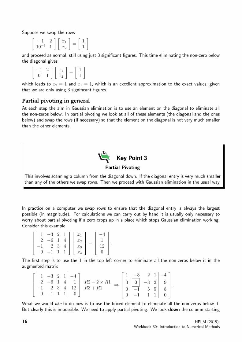
Suppose we swap the rows[−1 210−4 1

] [x1

x2

]=

[11

]and proceed as normal, still using just 3 significant figures. This time eliminating the non-zero belowthe diagonal gives[

−1 20 1

] [x1

x2

]=

[11

]which leads to x2 = 1 and x1 = 1, which is an excellent approximation to the exact values, giventhat we are only using 3 significant figures.

Partial pivoting in generalAt each step the aim in Gaussian elimination is to use an element on the diagonal to eliminate allthe non-zeros below. In partial pivoting we look at all of these elements (the diagonal and the onesbelow) and swap the rows (if necessary) so that the element on the diagonal is not very much smallerthan the other elements.

Key Point 3

Partial Pivoting

This involves scanning a column from the diagonal down. If the diagonal entry is very much smallerthan any of the others we swap rows. Then we proceed with Gaussian elimination in the usual way.

In practice on a computer we swap rows to ensure that the diagonal entry is always the largestpossible (in magnitude). For calculations we can carry out by hand it is usually only necessary toworry about partial pivoting if a zero crops up in a place which stops Gaussian elimination working.Consider this example

1 −3 2 12 −6 1 4−1 2 3 40 −1 1 1

x1

x2

x3

x4

=

−41120

.

The first step is to use the 1 in the top left corner to eliminate all the non-zeros below it in theaugmented matrix

1 −3 2 1 −42 −6 1 4 1−1 2 3 4 120 −1 1 1 0

R2− 2×R1R3 +R1

⇒

1 −3 2 1 −40 0 −3 2 9

0 −1 5 5 80 −1 1 1 0

.

What we would like to do now is to use the boxed element to eliminate all the non-zeros below it.But clearly this is impossible. We need to apply partial pivoting. We look down the column starting


®

at the diagonal entry and see that the two possible candidates for the swap are both equal to −1.Either will do so let us swap the second and fourth rows to give

1 −3 2 1 −40 −1 1 1 0

0 −1 5 5 80 0 −3 2 9

.

That was the partial pivoting step. Now we proceed with Gaussian elimination1 −3 2 1 −40 −1 1 1 0

0 −1 5 5 80 0 −3 2 9

R3−R2

⇒

1 −3 2 1 −40 −1 1 1 00 0 4 4 80 0 −3 2 9

.

The arithmetic is simpler if we cancel a factor of 4 out of the third row to give1 −3 2 1 −40 −1 1 1 00 0 1 1 20 0 −3 2 9

.

And the elimination phase is completed by removing the −3 from the final row as follows1 −3 2 1 −40 −1 1 1 0

0 0 1 1 2

0 0 −3 2 9

R4 + 3×R3

⇒

1 −3 2 1 −40 −1 1 1 00 0 1 1 20 0 0 5 15

.

This system is upper triangular so back substitution can be used now to work out that x4 = 3,x3 = −1, x2 = 2 and x1 = 1.

The Task below is a case in which partial pivoting is required.

[For a large system which can be solved by Gauss elimination see Engineering Example 1 on page62].

TaskTransform the matrix 1 −2 4

−3 6 −114 3 5

into upper triangular form using Gaussian elimination (with partial pivoting whennecessary).


17

Your solution

AnswerThe row operations required to eliminate the non-zeros below the diagonal in the first column are 1 −2 4

−3 6 −114 3 5

R2 + 3×R1R3− 4×R1

⇒

1 −2 40 0 10 11 −11

which puts a zero on the diagonal. We are forced to use partial pivoting and swapping the secondand third rows gives 1 −2 4

0 11 −110 0 1

which is in the required upper triangular form.

Key Point 4

When To Use Partial Pivoting

1. When carrying out Gaussian elimination on a computer, we would usually always swap rowsso that the element on the diagonal is as large (in magnitude) as possible. This helps stopthe growth of rounding error.

2. When doing hand calculations (not involving rounding) there are two reasons we might pivot

(a) If the element on the diagonal is zero, we have to swap rows so as to put a non-zero onthe diagonal.

(b) Sometimes we might swap rows so that there is a “nicer” non-zero number on thediagonal than there would be without pivoting. For example, if the number on thediagonal can be arranged to be a 1 then no awkward fractions will be introduced whenwe carry out row operations related to Gaussian elimination.


®

Exercises

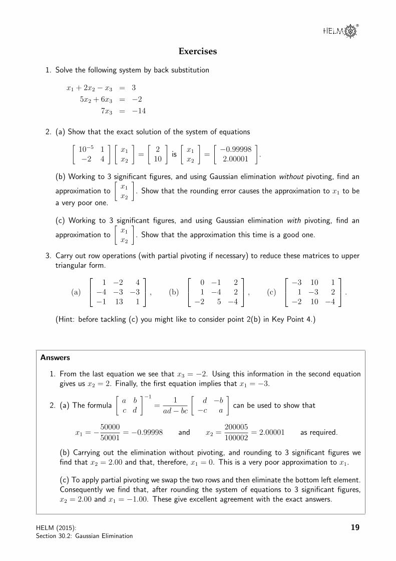
1. Solve the following system by back substitution

x1 + 2x2 − x3 = 3

5x2 + 6x3 = −27x3 = −14

2. (a) Show that the exact solution of the system of equations[10−5 1−2 4

] [x1

x2

]=

[210

]is

[x1

x2

]=

[−0.999982.00001

].

(b) Working to 3 significant figures, and using Gaussian elimination without pivoting, find an

approximation to

[x1

x2

]. Show that the rounding error causes the approximation to x1 to be

a very poor one.

(c) Working to 3 significant figures, and using Gaussian elimination with pivoting, find an

approximation to

[x1

x2

]. Show that the approximation this time is a good one.

3. Carry out row operations (with partial pivoting if necessary) to reduce these matrices to uppertriangular form.

(a)

1 −2 4−4 −3 −3−1 13 1

, (b)

0 −1 21 −4 2−2 5 −4

, (c)

−3 10 11 −3 2−2 10 −4

.

(Hint: before tackling (c) you might like to consider point 2(b) in Key Point 4.)

Answers

1. From the last equation we see that x3 = −2. Using this information in the second equationgives us x2 = 2. Finally, the first equation implies that x1 = −3.

2. (a) The formula

[a bc d

]−1

=1

ad− bc

[d −b−c a

]can be used to show that

x1 = −50000

50001= −0.99998 and x2 =

200005

100002= 2.00001 as required.

(b) Carrying out the elimination without pivoting, and rounding to 3 significant figures wefind that x2 = 2.00 and that, therefore, x1 = 0. This is a very poor approximation to x1.

(c) To apply partial pivoting we swap the two rows and then eliminate the bottom left element.Consequently we find that, after rounding the system of equations to 3 significant figures,x2 = 2.00 and x1 = −1.00. These give excellent agreement with the exact answers.


19

Answers

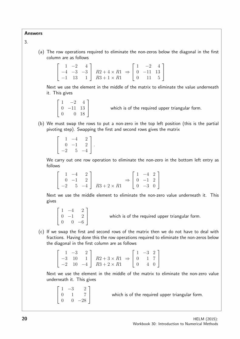
3.

(a) The row operations required to eliminate the non-zeros below the diagonal in the firstcolumn are as follows 1 −2 4

−4 −3 −3−1 13 1

R2 + 4×R1R3 + 1×R1

⇒

1 −2 40 −11 130 11 5

Next we use the element in the middle of the matrix to eliminate the value underneathit. This gives 1 −2 4

0 −11 130 0 18

which is of the required upper triangular form.

(b) We must swap the rows to put a non-zero in the top left position (this is the partialpivoting step). Swapping the first and second rows gives the matrix 1 −4 2

0 −1 2−2 5 −4

.

We carry out one row operation to eliminate the non-zero in the bottom left entry asfollows 1 −4 2

0 −1 2−2 5 −4

R3 + 2×R1

⇒

1 −4 20 −1 20 −3 0

Next we use the middle element to eliminate the non-zero value underneath it. Thisgives 1 −4 2

0 −1 20 0 −6


(c) If we swap the first and second rows of the matrix then we do not have to deal withfractions. Having done this the row operations required to eliminate the non-zeros belowthe diagonal in the first column are as follows 1 −3 2

−3 10 1−2 10 −4

R2 + 3×R1R3 + 2×R1

⇒

1 −3 20 1 70 4 0

Next we use the element in the middle of the matrix to eliminate the non-zero valueunderneath it. This gives 1 −3 2

0 1 70 0 −28



®

LU Decomposition��

��30.3

IntroductionIn this Section we consider another direct method for obtaining the solution of systems of equationsin the form AX = B.

�

�

�

�Prerequisites


• revise matrices and their use in systems ofequations

• revise determinants'

&

$

%

Learning OutcomesOn completion you should be able to . . .

• find an LU decomposition of simplematrices and apply it to solve systems ofequations

• determine when an LU decomposition isunavailable and when it is possible tocircumvent the problem

HELM (2015):Section 30.3: LU Decomposition

21

1. LU decompositionSuppose we have the system of equations

AX = B.

The motivation for an LU decomposition is based on the observation that systems of equationsinvolving triangular coefficient matrices are easier to deal with. Indeed, the whole point of Gaussianelimination is to replace the coefficient matrix with one that is triangular. The LU decomposition isanother approach designed to exploit triangular systems.We suppose that we can write

A = LU

where L is a lower triangular matrix and U is an upper triangular matrix. Our aim is to find L andU and once we have done so we have found an LU decomposition of A.

Key Point 5

An LU decomposition of a matrix A is the product of a lower triangular matrix and an uppertriangular matrix that is equal to A.

It turns out that we need only consider lower triangular matrices L that have 1s down the diagonal.Here is an example. Let

A =

1 2 43 8 142 6 13

= LU where L =

1 0 0L21 1 0L31 L32 1

and U =

U11 U12 U13

0 U22 U23

0 0 U33

.

Multiplying out LU and setting the answer equal to A gives U11 U12 U13

L21U11 L21U12 + U22 L21U13 + U23

L31U11 L31U12 + L32U22 L31U13 + L32U23 + U33

=

1 2 43 8 142 6 13

.

Now we use this to find the entries in L and U . Fortunately this is not nearly as hard as it might atfirst seem. We begin by running along the top row to see that

U11 = 1 , U12 = 2 , U13 = 4 .

Now consider the second row

L21U11 = 3 ∴ L21 × 1 = 3 ∴ L21 = 3 ,

L21U12 + U22 = 8 ∴ 3× 2 + U22 = 8 ∴ U22 = 2 ,

L21U13 + U23 = 14 ∴ 3× 4 + U23 = 14 ∴ U23 = 2 .


®

Notice how, at each step, the equation being considered has only one unknown in it, and otherquantities that we have already found. This pattern continues on the last row

L31U11 = 2 ∴ L31 × 1 = 2 ∴ L31 = 2 ,

L31U12 + L32U22 = 6 ∴ 2× 2 + L32 × 2 = 6 ∴ L32 = 1 ,

L31U13 + L32U23 + U33 = 13 ∴ (2× 4) + (1× 2) + U33 = 13 ∴ U33 = 3 .

We have shown that

A =

1 2 43 8 142 6 13

=

1 0 03 1 02 1 1

1 2 40 2 20 0 3

and this is an LU decomposition of A.

TaskFind an LU decomposition of

[3 1−6 −4

].

Your solution

AnswerLet [

3 1−6 −4

]= LU =

[1 0L21 1

] [U11 U12

0 U22

]=

[U11 U12

L21U11 L21U12 + U22

]then, comparing the left and right hand sides row by row implies that U11 = 3, U12 = 1, L21U11 = −6which implies L21 = −2 and L21U12 + U22 = −4 which implies that U22 = −2. Hence[

3 1−6 −4

]=

[1 0−2 1

] [3 10 −2

]is an LU decomposition of

[3 1−6 −4

].


23

TaskFind an LU decomposition of

3 1 6−6 0 −160 8 −17

.

Your solution

AnswerUsing material from the worked example in the notes we set 3 1 6

−6 0 −160 8 −17

=

U11 U12 U13

L21U11 L21U12 + U22 L21U13 + U23

L31U11 L31U12 + L32U22 L31U13 + L32U23 + U33

and comparing elements row by row we see that

U11 = 3, U12 = 1, U13 = 6,L21 = −2, U22 = 2, U23 = −4L31 = 0 L32 = 4 U33 = −1

and it follows that 3 1 6−6 0 −160 8 −17

=

1 0 0−2 1 00 4 1

3 1 60 2 −40 0 −1

is an LU decomposition of the given matrix.


®

2. Using LU decomposition to solve systems of equationsOnce a matrix A has been decomposed into lower and upper triangular parts it is possible to obtainthe solution to AX = B in a direct way. The procedure can be summarised as follows

• Given A, find L and U so that A = LU . Hence LUX = B.

• Let Y = UX so that LY = B. Solve this triangular system for Y .

• Finally solve the triangular system UX = Y for X.

The benefit of this approach is that we only ever need to solve triangular systems. The cost is thatwe have to solve two of them.

[Here we solve only small systems; a large system is presented in Engineering Example 1 on page 62.]

Example 6

Find the solution of X =

x1

x2

x3

of the system

1 2 43 8 142 6 13

x1

x2

x3

=

3134

.

Solution

• The first step is to calculate the LU decomposition of the coefficient matrix on the left-handside. In this case that job has already been done since this is the matrix we considered earlier.We found that

L =

1 0 03 1 02 1 1

, U =

1 2 40 2 20 0 3

.

• The next step is to solve LY = B for the vector Y =

y1y2y3

. That is we consider

LY =

1 0 03 1 02 1 1

y1y2y3

=

3134

= B

which can be solved by forward substitution. From the top equation we see that y1 = 3.The middle equation states that 3y1 + y2 = 13 and hence y2 = 4. Finally the bottom linesays that 2y1 + y2 + y3 = 4 from which we see that y3 = −6.


25

Solution (contd.)

• Now that we have found Y we finish the procedure by solving UX = Y for X. That is wesolve

UX =

1 2 40 2 20 0 3

x1

x2

x3

=

34−6

= Y

by using back substitution. Starting with the bottom equation we see that 3x3 = −6 soclearly x3 = −2. The middle equation implies that 2x2 + 2x3 = 4 and it follows that x2 = 4.The top equation states that x1 + 2x2 + 4x3 = 3 and consequently x1 = 3.

Therefore we have found that the solution to the system of simultaneous equations 1 2 43 8 142 6 13

x1

x2

x3

=

3134

is X =

34−2

.

TaskUse the LU decomposition you found earlier in the last Task (page 24) to solve 3 1 6−6 0 −160 8 −17

x1

x2

x3

=

0417

.

Your solution


®

Answer

We found earlier that the coefficient matrix is equal to LU =

1 0 0−2 1 00 4 1

3 1 60 2 −40 0 −1

.

First we solve LY = B for Y , we have 1 0 0−2 1 00 4 1

y1y2y3

=

0417

.

The top line implies that y1 = 0. The middle line states that −2y1 + y2 = 4 and therefore y2 = 4.The last line tells us that 4y2 + y3 = 17 and therefore y3 = 1.

Finally we solve UX = Y for X, we have 3 1 60 2 −40 0 −1

x1

x2

x3

=

041

.

The bottom line shows that x3 = −1. The middle line then shows that x2 = 0, and then the top

line gives us that x1 = 2. The required solution is X =

20−1

.

3. Do matrices always have an LU decomposition?No. Sometimes it is impossible to write a matrix in the form “lower triangular”×“upper triangular”.

Why not?An invertible matrix A has an LU decomposition provided that all its leading submatrices havenon-zero determinants. The kth leading submatrix of A is denoted Ak and is the k× k matrix foundby looking only at the top k rows and leftmost k columns. For example if

A =

1 2 43 8 142 6 13

then the leading submatrices are

A1 = 1, A2 =

[1 23 8

], A3 =

1 2 43 8 142 6 13

.

The fact that this matrix A has an LU decomposition can be guaranteed in advance because noneof these determinants is zero:

|A1| = 1,

|A2| = (1× 8)− (2× 3) = 2,

|A3| =∣∣∣∣ 8 146 13

∣∣∣∣− 2

∣∣∣∣ 3 142 13

∣∣∣∣+ 4

∣∣∣∣ 3 82 6

∣∣∣∣ = 20− (2× 11) + (4× 2) = 6

(where the 3× 3 determinant was found by expanding along the top row).


27

Example 7

Show that

1 2 32 4 51 3 4

does not have an LU decomposition.

Solution

The second leading submatrix has determinant equal to∣∣∣∣ 1 22 4

∣∣∣∣ = (1× 4)− (2× 2) = 0

which means that an LU decomposition is not possible in this case.

TaskWhich, if any, of these matrices have an LU decomposition?

(a) A =

[3 20 1

], (b) A =

[0 13 2

], (c) A =

1 −3 7−2 6 10 3 −2

.

Your solution

(a)

Answer

|A1| = 3 and |A2| = |A| = 3. Neither of these is zero, so A does have an LU decomposition.

Your solution

(b)

Answer

|A1| = 0 so A does not have an LU decomposition.

Your solution

(c)

Answer

|A1| = 1, |A2| = 6− 6 = 0, so A does not have an LU decomposition.


®

Can we get around this problem?Yes. It is always possible to re-order the rows of an invertible matrix so that all of the submatriceshave non-zero determinants.

Example 8

Reorder the rows of A =

1 2 32 4 51 3 4

so that the reordered matrix has an LU

decomposition.

Solution

Swapping the first and second rows does not help us since the second leading submatrix will stillhave a zero determinant. Let us swap the second and third rows and consider

B =

1 2 31 3 42 4 5

the leading submatrices are

B1 = 1, B2 =

[1 21 3

], B3 = B.

Now |B1| = 1, |B2| = 3× 1− 2× 1 = 1 and (expanding along the first row)

|B3| = 1(15− 16)− 2(5− 8) + 3(4− 6) = −1 + 6− 6 = −1.

All three of these determinants are non-zero and we conclude that B does have an LU decomposition.

TaskReorder the rows of A =

1 −3 7−2 6 10 3 −2

so that the reordered matrix has an

LU decomposition.

Your solution


29

AnswerLet us swap the second and third rows and consider

B =

1 −3 70 3 −2−2 6 1

the leading submatrices are

B1 = 1, B2 =

[1 −30 3

], B3 = B

which have determinants 1, 3 and 45 respectively. All of these are non-zero and we conclude thatB does indeed have an LU decomposition.

Exercises

1. Calculate LU decompositions for each of these matrices

(a) A =

[2 1−4 −6

](b) A =

2 1 −42 2 −26 3 −11

(c) A =

1 3 22 8 51 11 4

2. Check each answer in Question 1, by multiplying out LU to show that the product equals A.

3. Using the answers obtained in Question 1, solve the following systems of equations.

(a)

[2 1−4 −6

] [x1

x2

]=

[12

]

(b)

2 1 −42 2 −26 3 −11

x1

x2

x3

=

4011

(c)

1 3 22 8 51 11 4

x1

x2

x3

=

230

4. Consider A =

1 6 22 12 5−1 −3 −1

(a) Show that A does not have an LU decomposition.

(b) Re-order the rows of A and find an LU decomposition of the new matrix.

(c) Hence solve

x1 + 6x2 + 2x3 = 9

2x1 + 12x2 + 5x3 = −4−x1 − 3x2 − x3 = 17


®

Answers

1. (a) We let[2 1−4 −6

]= LU =

[1 0

L21 1

] [U11 U12

0 U22

]=

[U11 U12

L21U11 L21U12 + U22

].

Comparing the left-hand and right-hand sides row by row gives us that U11 = 2, U12 = 1,L21U11 = −4 which implies that L21 = −2 and, finally, L21U12 + U22 = −6 from whichwe see that U22 = −4. Hence[

2 1−4 −6

]=

[1 0−2 1

] [2 10 −4

]is an LU decomposition of the given matrix.

(b) We let 2 1 −42 2 −26 3 −11

= LU =

U11 U12 U13

L21U11 L21U12 + U22 L21U13 + U23

L31U11 L31U12 + L32U22 L31U13 + L32U23 + U33

.

Looking at the top row we see that U11 = 2, U12 = 1 and U13 = −4. Now, from thesecond row, L21 = 1, U22 = 1 and U23 = 2. The last three unknowns come from thebottom row: L31 = 3, L32 = 0 and U33 = 1. Hence 2 1 −4

2 2 −26 3 −11

=

1 0 01 1 03 0 1

2 1 −40 1 20 0 1


(c) We let 1 3 22 8 51 11 4

= LU =

U11 U12 U13

L21U11 L21U12 + U22 L21U13 + U23

L31U11 L31U12 + L32U22 L31U13 + L32U23 + U33

.

Looking at the top row we see that U11 = 1, U12 = 3 and U13 = 2. Now, from thesecond row, L21 = 2, U22 = 2 and U23 = 1. The last three unknowns come from thebottom row: L31 = 1, L32 = 4 and U33 = −2. Hence 1 3 2

2 8 51 11 4

=

1 0 02 1 01 4 1

1 3 20 2 10 0 −2


2. Direct multiplication provides the necessary check.


31

Answers

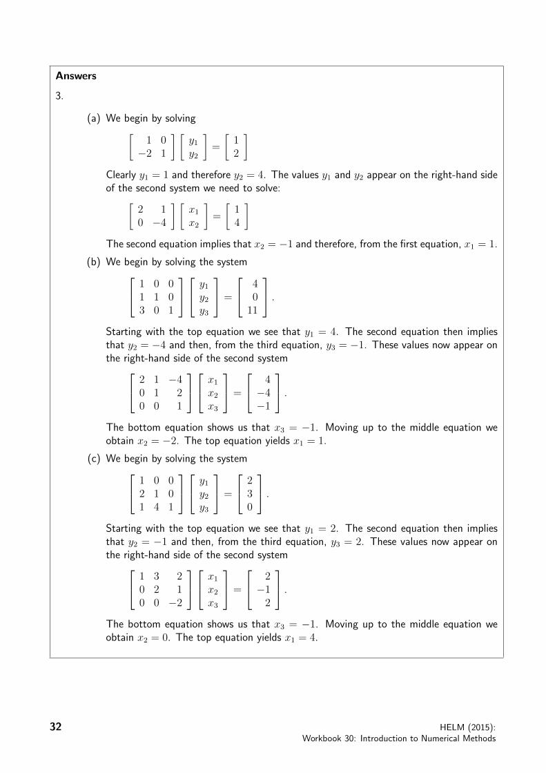
3.

(a) We begin by solving[1 0−2 1

] [y1y2

]=

[12

]Clearly y1 = 1 and therefore y2 = 4. The values y1 and y2 appear on the right-hand sideof the second system we need to solve:[

2 10 −4

] [x1

x2

]=

[14

]The second equation implies that x2 = −1 and therefore, from the first equation, x1 = 1.

(b) We begin by solving the system 1 0 01 1 03 0 1

y1y2y3

=

4011

.

Starting with the top equation we see that y1 = 4. The second equation then impliesthat y2 = −4 and then, from the third equation, y3 = −1. These values now appear onthe right-hand side of the second system 2 1 −4

0 1 20 0 1

x1

x2

x3

=

4−4−1

.

The bottom equation shows us that x3 = −1. Moving up to the middle equation weobtain x2 = −2. The top equation yields x1 = 1.

(c) We begin by solving the system 1 0 02 1 01 4 1

y1y2y3

=

230

.

Starting with the top equation we see that y1 = 2. The second equation then impliesthat y2 = −1 and then, from the third equation, y3 = 2. These values now appear onthe right-hand side of the second system 1 3 2

0 2 10 0 −2

x1

x2

x3

=

2−12

.

The bottom equation shows us that x3 = −1. Moving up to the middle equation weobtain x2 = 0. The top equation yields x1 = 4.


®

Answers

4.

(a) The second leading submatrix has determinant 1× 12− 6× 2 = 0 and this implies thatA has no LU decomposition.

(b) Swapping the second and third rows gives

1 6 2−1 −3 −12 12 5

. We let

1 6 2−1 −3 −12 12 5

= LU =

U11 U12 U13

L21U11 L21U12 + U22 L21U13 + U23

L31U11 L31U12 + L32U22 L31U13 + L32U23 + U33

.

Looking at the top row we see that U11 = 1, U12 = 6 and U13 = 2. Now, from thesecond row, L21 = −1, U22 = 3 and U23 = 1. The last three unknowns come from thebottom row: L31 = 2, L32 = 0 and U33 = 1. Hence 1 6 2

−1 −3 −12 12 5

=

1 0 0−1 1 02 0 1

1 6 20 3 10 0 1


(c) We begin by solving the system 1 0 0−1 1 02 0 1

y1y2y3

=

917−4

.

(Note that the second and third rows of the right-hand side vector have been swappedtoo.) Starting with the top equation we see that y1 = 9. The second equation thenimplies that y2 = 26 and then, from the third equation, y3 = −22. These values nowappear on the right-hand side of the second system 1 6 2

0 3 10 0 1

x1

x2

x3

=

926−22

.

The bottom equation shows us that x3 = −22. Moving up to the middle equation weobtain x2 = 16. The top equation yields x1 = −43.


33

Matrix Norms��

��30.4

IntroductionA matrix norm is a number defined in terms of the entries of the matrix. The norm is a usefulquantity which can give important information about a matrix.

'

&

$

%

PrerequisitesBefore starting this Section you should . . .

• be familiar with matrices and their use inwriting systems of equations

• revise material on matrix inverses, be able tofind the inverse of a 2× 2 matrix, and knowwhen no inverse exists

• revise Gaussian elimination and partialpivoting

• be aware of the discussion of ill-conditionedand well-conditioned problems earlier inSection 30.1#

"

!Learning Outcomes


• calculate norms and condition numbers ofsmall matrices

• adjust certain systems of equations with aview to better conditioning


®

1. Matrix normsThe norm of a square matrix A is a non-negative real number denoted ‖A‖. There are severaldifferent ways of defining a matrix norm, but they all share the following properties:

1. ‖A‖ ≥ 0 for any square matrix A.

2. ‖A‖ = 0 if and only if the matrix A = 0.

3. ‖kA‖ = |k| ‖A‖, for any scalar k.

4. ‖A+B‖ ≤ ‖A‖+ ‖B‖.

5. ‖AB‖ ≤ ‖A‖ ‖B‖.

The norm of a matrix is a measure of how large its elements are. It is a way of determining the“size” of a matrix that is not necessarily related to how many rows or columns the matrix has.

Key Point 6

Matrix Norm

The norm of a matrix is a real number which is a measure of the magnitude of the matrix.

Anticipating the places where we will use norms later, it is sufficient at this stage to restrict ourattention to matrices with only real-valued entries. There is no need to consider complex numbersat this stage.

In the definitions of norms below we will use this notation for the elements of an n × n matrix Awhere

A =

a11 a12 a13 . . . a1na21 a22 a23 . . . a2na31 a32 a33 . . . a3n

......

.... . .

...an1 an2 an3 . . . ann

The subscripts on a have the row number first, then the column number. The fact that

arc

is reminiscent of the word “arc” may be a help in remembering how the notation goes.

In this Section we will define three commonly used norms. We distinguish them with a subscript. Allthree of them satisfy the five conditions listed above, but we will not concern ourselves with verifyingthat fact.

HELM (2015):Section 30.4: Matrix Norms

35

The 1-norm

‖A‖1 = max1≤j≤n

(n∑

i=1

|aij|

)(the maximum absolute column sum). Put simply, we sum the absolute values down each columnand then take the biggest answer.

Example 9Calculate the 1-norm of A =

[1 −7−2 −3

].

Solution

The absolute column sums of A are 1 + | − 2| = 1 + 2 = 3 and | − 7|+ | − 3| = 7 + 3 = 10. Thelarger of these is 10 and therefore ‖A‖1 = 10.

Example 10

Calculate the 1-norm of B =

5 −4 2−1 2 3−2 1 0

.

Solution

Summing down the columns of B we find that

‖B‖1 = max (5 + 1 + 2, 4 + 2 + 1, 2 + 3 + 0)

= max (8, 7, 5)

= 8

Key Point 7

The 1-norm of a square matrix is the maximum of the absolute column sums.(A useful reminder is that “1” is a tall, thin character and a column is a tall, thin quantity.)


®

The infinity-norm

‖A‖∞ = max1≤i≤n

(n∑

j=1

|aij|

)(the maximum absolute row sum). Put simply, we sum the absolute values along each row and thentake the biggest answer.

Example 11Calculate the infinity-norm of A =

[1 −7−2 −3

].

Solution

The absolute row sums of A are 1+ | − 7| = 8 and | − 2|+ | − 3| = 5. The larger of these is 8 andtherefore ‖A‖∞ = 8.

Example 12

Calculate the infinity-norm of B =

5 −4 2−1 2 3−2 1 0

.

Solution

Summing along the rows of B we find that

‖B‖∞ = max (5 + 4 + 2, 1 + 2 + 3, 2 + 1 + 0)

= max (11, 6, 3)

= 11

Key Point 8

The infinity-norm of a square matrix is the maximum of the absolute row sums.(A useful reminder is that “∞” is a short, wide character and a row is a short, wide quantity.)


37

The Euclidean norm

‖A‖E =

√√√√ n∑i=1

n∑j=1

(aij)2

(the square root of the sum of all the squares). This is similar to ordinary “Pythagorean” lengthwhere the size of a vector is found by taking the square root of the sum of the squares of all theelements.

Example 13Calculate the Euclidean norm of A =

[1 −7−2 −3

].

Solution

‖A‖E =√

12 + (−7)2 + (−2)2 + (−3)2

=√1 + 49 + 4 + 9

=√63 ≈ 7.937.

Example 14

Calculate the Euclidean norm of B =

5 −4 2−1 2 3−2 1 0

.

Solution

‖B‖E =√25 + 16 + 4 + 1 + 4 + 9 + 4 + 1 + 0

=√64

= 8.

Key Point 9

The Euclidean norm of a square matrix is the square root of the sum of all the squares of theelements.


®

TaskCalculate the norms indicated of these matrices

A =

[2 −83 1

](1-norm), B =

3 6 −13 1 02 4 −7

(infinity-norm),

C =

1 7 34 −2 −2−2 −1 1

(Euclidean-norm).

Your solution

Answer

‖A‖1 = max(2 + 3, 8 + 1) = 9,

‖B‖∞ = max(3 + 6 + 1, 3 + 1 + 0, 2 + 4 + 7) = 13,

‖C‖E =√

12 + 72 + 32 + 42 + (−2)2 + (−2)2 + (−2)2 + (−1)2 + 12

=√89 ≈ 9.434

Other normsAny definition you can think of which satisifes the five conditions mentioned at the beginning of thisSection is a definition of a norm. There are many many possibilities, but the three given above areamong the most commonly used.


39

2. Condition numbersThe condition number of an invertible matrix A is defined to be

κ(A) = ‖A‖ ‖A−1‖.

This quantity is always bigger than (or equal to) 1.We must use the same type of norm twice on the right-hand side of the above equation. Sometimesthe notation is adjusted to make it clear which norm is being used, for example if we use the infinitynorm we might write

κ∞(A) = ‖A‖∞‖A−1‖∞.

Example 15Use the norm indicated to calculate the condition number of the given matrices.

(a) A =

[2 31 −1

]; 1-norm. (b) A =

[2 31 −1

]; Euclidean norm.

(c) B =

−3 0 00 4 00 0 2

; infinity-norm.

Solution

(a) ‖A‖1 = max(2 + 1, 3 + 1) = 4,

A−1 =1

−2− 3

[−1 −3−1 2

]=

15

35

15−25

∴ ‖A−1‖1 = max(1

5+ 1

5, 35+ 2

5) = 1.

Therefore κ1(A) = ‖A‖1 ‖A−1‖1 = 4× 1 = 4.

(b) ‖A‖E =√

22 + 32 + 12 + (−1)2 =√15. We can re-use A−1 from above to see that

‖A−1‖E =

√(1

5

)2

+

(3

5

)2

+

(1

5

)2

+

(−25

)2

=

√15

25.

Therefore κE(A) = ‖A‖E ‖A−1‖E =√15×

√15

25=

15√25

=15

5= 3.

(c) ‖B‖∞ = max(3, 4, 2) = 4.

B−1 =

−13

0 00 1

40

0 0 12

so ‖B−1‖∞ = max(1

3, 14, 12) = 1

2. Therefore κ∞(B) = ‖B‖∞ ‖B−1‖∞ = 4× 1

2= 2.


®

TaskCalculate the condition numbers of these matrices, using the norm indicated

A =

[2 −83 1

](1-norm), B =

[3 61 0

](infinity-norm).

Your solution

Answer

A−1 =1

2 + 24

[1 8−3 2

]so κ1(A) = ‖A‖1‖A−1‖1 = max(5, 9)×max( 4

26, 1026) = 9× 10

26= 45

13.

B−1 =1

0− 6

[0 −6−1 3

]so κ∞(B) = ‖B‖∞‖B−1‖∞ = max(9, 1)×max(1, 4

6) = 9.

Condition numbers and conditioningAs the name might suggest, the condition number gives us information regarding how well-conditioned a problem is. Consider this example[

1 104

−1 2

] [x1x2

]=

[104

1

].

It is not hard to verify that the exact solution to this problem is

[x1x2

]=

10000

10002

10001

10002

=

[0.999800...0.999900...

].

Example 16Using the 1-norm find the condition number of

[1 104

−1 2

].

Solution

Firstly, ‖A‖1 = 2 + 104. Also

A−1=1

2 + 104

[2 −1041 1

]∴ ‖A−1‖1=

1

2 + 104(1 + 104). Hence κ1(A)=1 + 104=10001.


41

The fact that this number is large is the indication that the problem involving A is an ill-conditionedone. Suppose we consider finding its solution by Gaussian elimination, using 3 significant figuresthroughout. Eliminating the non-zero in the bottom left corner gives[

1 104

0 104

] [x1x2

]=

[104

104

].

which implies that x2 = 1 and x1 = 0. This is a poor approximation to the true solution and partialpivoting will not help. We have altered the problem by a relatively tiny amount (that is, by neglecting

the fourth significant figure) and the result

[x1x2

]has changed by a large amount. In other words

the problem is ill-conditioned.

One way that systems of equations can be made better conditioned is to fix things so that all the

rows have largest elements that are about the same size. In the matrix A =

[1 104

−1 2

]the first

row’s largest element is 104, the second row has largest element equal to 2. This is not a happysituation.

If we divide the first equation through by 104 then we have[10−4 1−1 2

] [x1x2

]=

[11

]then the top row has largest entry equal to 1, and the bottom row still has 2 as its largest entry.These two values are of comparable size.

The solution to the system was found via pivoting (using 3 significant figures) in the Section con-cerning Gaussian elimination to be x1 = x2 = 1, a pretty good approximation to the exact values.The matrix in this second version of the problem is much better conditioned.

Example 17Using the 1-norm find the condition number of

[10−4 1−1 2

].

Solution

The 1-norm of A is easily seen to be ‖A‖1 = 3. We also need

A−1 =1

2× 10−4 + 1

[2 −11 10−4

]∴ ‖A−1‖1 =

3

2× 10−4 + 1.

Hence

κ1(A) =9

2× 10−4 + 1≈ 8.998

This condition number is much smaller than the earlier value of 10001, and this shows us that thesecond version of the system of equations is better conditioned.


®

Exercises

1. Calculate the indicated norm of the following matrices

(a) A =

[2 −21 −3

]; 1-norm.

(b) A =

[2 −21 −3

]; infinity-norm.

(c) B =

[2 −31 −2

]; Euclidean norm.

(d) C =

1 −2 31 5 62 −1 3

; infinity-norm.

(e) C =

1 −2 31 5 62 −1 3

; 1-norm.

2. Use the norm indicated to calculate the condition number of the given matrices.

(a) D =

[4 −26 0

]; 1-norm.

(b) E =

[−1 54 2

]; Euclidean norm.

(c) F =

6 0 00 4 00 0 1

; infinity-norm.

3. Why is it not sensible to ask what the condition number of

[−1 32 −6

]is?

4. Verify that the inverse of G =

2 4 −12 5 2−1 −1 1

is1

5

−7 3 −134 −1 6−3 2 −2

.Hence find the condition number of G using the 1-norm.

5. (a) Calculate the condition number (use any norm you choose) of the coefficient matrix ofthe system[

1 104

2 3

] [x1x2

]=

[13

]and hence conclude that the problem as stated is ill-conditioned.

(b) Multiply one of the equations through by a suitably chosen constant so as to make thesystem better conditioned. Calculate the condition number of the coefficient matrix inyour new system of equations.


43

Answers

1. (a) ‖A‖1 = max(2 + 1, 2 + 3) = 5.

(b) ‖A‖∞ = max(2 +−2, 1 + 3) = 4.

(c) ‖B‖E =√4 + 9 + 1 + 4 =

√18

(d) ‖C‖∞ = max(1 + 2 + 3, 1 + 5 + 6, 2 + 1 + 3) = 12.

(e) ‖C‖1 = max(1 + 1 + 2, 2 + 5 + 1, 3 + 6 + 3) = 12.

2. (a) To work out the condition number we need to find

D−1 =1

12

[0 2−6 4

].

Given this we work out the condition number as the product of two norms as follows

κ1(D) = ‖D‖1‖D−1‖1 = 10× 12= 5.

(b) To work out the condition number we need to find

E−1 =1

−22

[2 −5−4 −1

].

Given this we work out the condition number as the product of two norms as follows

κE(E) = ‖E‖E‖E−1‖E = 6.782330× 0.308288 = 2.090909.


(c) Here F−1 =

16

0 00 1

40

0 0 1

so that κ∞(F ) = ‖F‖∞‖F−1‖∞ = 6× 1 = 6.

3. The matrix is not invertible.


®

Answers

4. Verification is done by a direct multiplication to show that GG−1 =

1 0 00 1 00 0 1

.

Using the 1-norm we find that κ1(G) = ‖G‖1‖G−1‖1 = 10× 215= 42.

5.

(a) The inverse of the coefficient matrix is

1

3− 2× 104

[3 −104−2 1

]=−1

19997

[3 −10000−2 1

].

Using the 1-norm the condition number of the coefficient matrix is

(3 + 104)× 1

19997(1 + 104) = 5002.75

to 6 significant figures. This is a large condition number, and the given problem is notwell-conditioned.

(b) Now we multiply the top equation through by 10−4 so that the system of equationsbecomes[

10−4 12 3

] [x1x2

]=

[13

]and the inverse of this new coefficient matrix is

1

3× 10−4 − 2

[3 −1−2 10−4

]=−1

1.9997

[3 −1−2 .0001

].

Using the 1-norm again we find that the condition number of the new coefficient matrixis

4× 1

1.9997(5) = 10.0015

to 6 significant figures. This much smaller condition number implies that the secondproblem is better conditioned.


45

Iterative Methods forSystems of Equations

��

��30.5

IntroductionThere are occasions when direct methods (like Gaussian elimination or the use of an LU decompo-sition) are not the best way to solve a system of equations. An alternative approach is to use aniterative method. In this Section we will discuss some of the issues involved with iterative methods.

'

&

$

%Prerequisites


• revise matrices, especially the material in8

• revise determinants

• revise matrix norms#

"

!Learning Outcomes


• approximate the solutions of simplesystems of equations by iterative methods

• assess convergence properties of iterativemethods


®

1. Iterative methodsSuppose we have the system of equations

AX = B.

The aim here is to find a sequence of approximations which gradually approach X. We will denotethese approximations

X(0), X(1), X(2), . . . , X(k), . . .

where X(0) is our initial “guess”, and the hope is that after a short while these successive iterateswill be so close to each other that the process can be deemed to have converged to the requiredsolution X.

Key Point 10

An iterative method is one in which a sequence of approximations (or iterates) is produced. Themethod is successful if these iterates converge to the true solution of the given problem.

It is convenient to split the matrix A into three parts. We write

A = L+D + U

where L consists of the elements of A strictly below the diagonal and zeros elsewhere; D is a diagonalmatrix consisting of the diagonal entries of A; and U consists of the elements of A strictly abovethe diagonal. Note that L and U here are not the same matrices as appeared in the LUdecomposition! The current L and U are much easier to find.For example[

3 −42 1

]︸︷︷︸ =

[0 02 0

]︸︷︷︸ +

[3 00 1

]︸︷︷︸ +

[0 −40 0

]︸︷︷︸

↑ ↑ ↑ ↑A = L + D + U

and 2 −6 13 −2 04 −1 7

︸︷︷︸

=

0 0 03 0 04 −1 0

︸︷︷︸

+

2 0 00 −2 00 0 7

︸︷︷︸

+

0 −6 10 0 00 0 0

︸︷︷︸

↑ ↑ ↑ ↑A = L + D + U

HELM (2015):Section 30.5: Iterative Methods for Systems of Equations

47

and, more generally for 3× 3 matrices • • •• • •• • •

︸︷︷︸

=

0 0 0• 0 0• • 0

︸︷︷︸

+

• 0 00 • 00 0 •

︸︷︷︸

+

0 • •0 0 •0 0 0

︸︷︷︸

.

↑ ↑ ↑ ↑A = L + D + U.

The Jacobi iterationThe simplest iterative method is called Jacobi iteration and the basic idea is to use the A =L+D + U partitioning of A to write AX = B in the form

DX = −(L+ U)X +B.

We use this equation as the motivation to define the iterative process

DX(k+1) = −(L+ U)X(k) +B

which gives X(k+1) as long as D has no zeros down its diagonal, that is as long as D is invertible.This is Jacobi iteration.

Key Point 11

The Jacobi iteration for approximating the solution of AX = B where A = L +D + U is givenby

X(k+1) = −D−1(L+ U)X(k) +D−1B

Example 18

Use the Jacobi iteration to approximate the solution X =

x1

x2

x3

of 8 2 43 5 12 1 4

x1

x2

x3

=

−164−12

.

Use the initial guess X(0) =

000

.


®

Solution

In this case D =

8 0 00 5 00 0 4

and L+ U =

0 2 43 0 12 1 0

.

First iteration.The first iteration is DX(1) = −(L+ U)X(0) +B, or in full 8 0 0

0 5 00 0 4

x

(1)1

x(1)2

x(1)3

=

0 −2 −4−3 0 −1−2 −1 0

x

(0)1

x(0)2

x(0)3

+

−164−12

=

−164−12

,

since the initial guess was x(0)1 = x

(0)2 = x

(0)3 = 0.

Taking this information row by row we see that

8x(1)1 = −16 ∴ x

(1)1 = −2

5x(1)2 = 4 ∴ x

(1)2 = 0.8

4x(1)3 = −12 ∴ x

(1)3 = −3

Thus the first Jacobi iteration gives us X(1) =

x(1)1

x(1)2

x(1)3

=

−20.8−3

as an approximation to X.

Second iteration.The second iteration is DX(2) = −(L+ U)X(1) +B, or in full 8 0 0

0 5 00 0 4

x

(2)1

x(2)2

x(2)3

=

0 −2 −4−3 0 −1−2 −1 0

x

(1)1

x(1)2

x(1)3

+

−164−12

.


8x(2)1 = −2x(1)

2 − 4x(1)3 − 16 = −2(0.8)− 4(−3)− 16 = −5.6 ∴ x

(2)1 = −0.7

5x(2)2 = −3x(1)

1 − x(1)3 + 4 = −3(−2)− (−3) + 4 = 13 ∴ x

(2)2 = 2.6

4x(2)3 = −2x(1)

1 − x(1)2 − 12 = −2(−2)− 0.8− 12 = −8.8 ∴ x

(2)3 = −2.2

Therefore the second iterate approximating X is X(2) =

x(2)1

x(2)2

x(2)3

=

−0.72.6−2.2

.


49

Solution (contd.)

Third iteration.The third iteration is DX(3) = −(L+ U)X(2) +B, or in full 8 0 0

0 5 00 0 4

x

(3)1

x(3)2

x(3)3

=

0 −2 −4−3 0 −1−2 −1 0

x

(2)1

x(2)2

x(2)3

+

−164−12


8x(3)1 = −2x(2)

2 − 4x(2)3 − 16 = −2(2.6)− 4(−2.2)− 16 = −12.4 ∴ x

(3)1 = −1.55

5x(3)2 = −3x(2)

1 − x(2)3 + 4 = −3(−0.7)− (2.2) + 4 = 8.3 ∴ x

(3)2 = 1.66

4x(3)3 = −2x(2)

1 − x(2)2 − 12 = −2(−0.7)− 2.6− 12 = −13.2 ∴ x

(3)3 = −3.3

Therefore the third iterate approximating X is X(3) =

x(3)1

x(3)2

x(3)3

=

−1.551.66−3.3

.

More iterations ...Three iterations is plenty when doing these calculations by hand! But the repetitive nature of theprocess is ideally suited to its implementation on a computer. It turns out that the next few iteratesare

X(4) =

−0.7652.39−2.64

, X(5) =

−1.2771.787−3.215

, X(6) =

−0.8392.209−2.808

,

to 3 d.p. Carrying on even further X(20) =

x(20)1

x(20)2

x(20)3

=

−0.99592.0043−2.9959

, to 4 d.p. After about 40

iterations successive iterates are equal to 4 d.p. Continuing the iteration even further causes theiterates to agree to more and more decimal places. The method converges to the exact answer

X =

−12−3

.

The following Task involves calculating just two iterations of the Jacobi method.


®

TaskCarry out two iterations of the Jacobi method to approximate the solution of 4 −1 −1

−1 4 −1−1 −1 4

x1

x2

x3

=

123

with the initial guess X(0) =

111

.

Your solution

First iteration:

AnswerThe first iteration is DX(1) = −(L+ U)X(0) +B, that is, 4 0 0

0 4 00 0 4

x

(1)1

x(1)2

x(1)3

=

0 1 11 0 11 1 0

x

(0)1

x(0)2

x(0)3

+

123

from which it follows that X(1) =

0.751

1.25

.

Your solution

Second iteration:


51

AnswerThe second iteration is DX(1) = −(L+ U)X(0) +B, that is, 4 0 0

0 4 00 0 4

x

(2)1

x(2)2

x(2)3

=

0 1 11 0 11 1 0

x

(0)1

x(0)2

x(0)3

+

123


0.81251

1.1875

.

Notice that at each iteration the first thing we do is get a new approximation for x1 and then wecontinue to use the old approximation to x1 in subsequent calculations for that iteration! Only atthe next iteration do we use the new value. Similarly, we continue to use an old approximation to x2

even after we have worked out a new one. And so on.

Given that the iterative process is supposed to improve our approximations why not use the bettervalues straight away? This observation is the motivation for what follows.

Gauss-Seidel iterationThe approach here is very similar to that used in Jacobi iteration. The only difference is that we usenew approximations to the entries of X as soon as they are available. As we will see in the Examplebelow, this means rearranging (L+D + U)X = B slightly differently from what we did for Jacobi.We write

(D + L)X = −UX +B

and use this as the motivation to define the iteration

(D + L)X(k+1) = −UX(k) +B.

Key Point 12

The Gauss-Seidel iteration for approximating the solution of AX = B is given by

X(k+1) = −(D + L)−1UX(k) + (D + L)−1B

Example 19 which follows revisits the system of equations we saw earlier in this Section in Example18.


®

Example 19

Use the Gauss-Seidel iteration to approximate the solution X =

x1

x2

x3

of 8 2 43 5 12 1 4

x1

x2

x3

=

−164−12

. Use the initial guess X(0) =

000

.

Solution

In this case D + L =

8 0 03 5 02 1 4

and U =

0 2 40 0 10 0 0

.

First iteration.

The first iteration is (D + L)X(1) = −UX(0) +B, or in full

8 0 03 5 02 1 4

x

(1)1

x(1)2

x(1)3

=

0 −2 −40 0 −10 0 0

x

(0)1

x(0)2

x(0)3

+

−164−12

=

−164−12

,

since the initial guess was x(0)1 = x

(0)2 = x

(0)3 = 0.


8x(1)1 = −16 ∴ x

(1)1 = −2

3x(1)2 + 5x

(1)2 = 4 ∴ 5x

(1)2 = −3(−2) + 4 ∴ x

(1)2 = 2

2x(1)1 + x

(1)2 + 4x

(1)3 = −12 ∴ 4x

(1)3 = −2(−2)− 2− 12 ∴ x

(1)3 = −2.5

(Notice how the new approximations to x1 and x2 were used immediately after they were found.)

Thus the first Gauss-Seidel iteration gives us X(1) =

x(1)1

x(1)2

x(1)3

=

−22−2.5

as an approximation to

X.


53

Solution

Second iteration.The second iteration is (D + L)X(2) = −UX(1) +B, or in full 8 0 0

3 5 02 1 4

x

(2)1

x(2)2

x(2)3

=

0 −2 −40 0 −10 0 0

x

(1)1

x(1)2

x(1)3

+

−164−12


8x(2)1 = −2x(1)

2 − 4x(1)3 − 16 ∴ x

(2)1 = −1.25

3x(2)1 + 5x

(2)2 = −x(1)

3 + 4 ∴ x(2)2 = 2.05

2x(2)1 + x

(2)2 + 4x

(2)3 = −12 ∴ x

(2)3 = −2.8875

Therefore the second iterate approximating X is X(2) =

x(2)1

x(2)2

x(2)3

=

−1.252.05−2.8875

.

Third iteration.The third iteration is (D + L)X(3) = −UX(2) +B, or in full 8 0 0

3 5 02 1 4

x

(3)1

x(3)2

x(3)3

=

0 −2 −40 0 −10 0 0

x

(2)1

x(2)2

x(2)3

+

−164−12

.


8x(3)1 = −2x(2)

2 − 4x(2)3 − 16 ∴ x

(3)1 = −1.0687

3x(3)1 + 5x

(3)2 = −x(2)

3 + 4 ∴ x(3)2 = 2.0187

2x(3)1 + x

(3)2 + 4x

(3)3 = −12 ∴ x

(3)3 = −2.9703

to 4 d.p. Therefore the third iterate approximating X is

X(3) =

x(3)1

x(3)2

x(3)3

=

−1.06872.0187−2.9703

.

More iterations ...

Again, there is little to be learned from pushing this further by hand. Putting the procedure on acomputer and seeing how it progresses is instructive, however, and the iteration continues as follows:


®

X(4) =

−1.01952.0058−2.9917

, X(5) =

−1.00562.0017−2.9976

, X(6) =

−1.00162.0005−2.9993

,

X(7) =

−1.00052.0001−2.9998

, X(8) =

−1.00012.0000−2.9999

, X(9) =

−1.00002.0000−3.0000

(to 4 d.p.). Subsequent iterates are equal to X(9) to this number of decimal places. The Gauss-Seideliteration has converged to 4 d.p. in 9 iterations. It took the Jacobi method almost 40 iterations toachieve this!

TaskCarry out two iterations of the Gauss-Seidel method to approximate the solutionof 4 −1 −1

−1 4 −1−1 −1 4

x1

x2

x3

=

123

with the initial guess X(0) =

111

.

Your solution

First iteration

AnswerThe first iteration is (D + L)X(1) = −UX(0) +B, that is, 4 0 0

−1 4 0−1 −1 4

x

(1)1

x(1)2

x(1)3

=

0 1 10 0 10 0 0

x

(0)1

x(0)2

x(0)3

+

123


0.750.93751.1719

.


55

Your solution

Second iteration

AnswerThe second iteration is (D + L)X(1) = −UX(0) +B, that is, 4 0 0

−1 4 0−1 −1 4

x

(2)1

x(2)2

x(2)3

=

0 1 10 0 10 0 0

x

(1)1

x(1)2

x(1)3

+

123


0.77730.98731.1912

.

2. Do these iterative methods always work?No. It is not difficult to invent examples where the iteration fails to approach the solution of AX = B.The key point is related to matrix norms seen in the preceding Section.The two iterative methods we encountered above are both special cases of the general form

X(k+1) = MX(k) +N.

1. For the Jacobi method we choose M = −D−1(L+ U) and N = D−1B.

2. For the Gauss-Seidel method we choose M = −(D + L)−1U and N = (D + L)−1B.

The following Key Point gives the main result.

Key Point 13

For the iterative process X(k+1) = MX(k)+N the iteration will converge to a solution if the normof MMM is less than 1.


®

Care is required in understanding what Key Point 13 says. Remember that there are lots of differentways of defining the norm of a matrix (we saw three of them). If you can find a norm (any norm)such that the norm of M is less than 1, then the iteration will converge. It doesn’t matter if thereare other norms which give a value greater than 1, all that matters is that there is one norm that isless than 1.

Key Point 13 above makes no reference to the starting “guess” X(0). The convergence of the iterationis independent of where you start! (Of course, if we start with a really bad initial guess then we canexpect to need lots of iterations.)

TaskShow that the Jacobi iteration used to approximate the solution of 4 −1 −1

1 −5 −2−1 0 2

x1

x2

x3

=

123

is certain to converge. (Hint: calculate the norm of −D−1(L+ U).)

Your solution

AnswerThe Jacobi iteration matrix is

−D−1(L+ U) =

4 0 00 −5 00 0 2

−1 0 1 1−1 0 21 0 0

=

0.25 0 00 −0.2 00 0 0.5

0 1 1−1 0 21 0 0

=

0 0.25 0.25−0.2 0 0.40.5 0 0

and the infinity norm of this matrix is the maximum of 0.25 + 0.25, 0.2 + 0.4 and 0.5, that is

‖ −D−1(L+ U)‖∞ = 0.6

which is less than 1 and therefore the iteration will converge.


57

Guaranteed convergenceIf the matrix has the property that it is strictly diagonally dominant, which means that the diagonalentry is larger in magnitude than the absolute sum of the other entries on that row, then both Jacobiand Gauss-Seidel are guaranteed to converge. The reason for this is that if A is strictly diagonallydominant then the iteration matrix M will have an infinity norm that is less than 1.

A small system is the subject of Example 20 below. A large system with slow convergence is thesubject of Engineering Example 1 on page 62.

Example 20

Show that A =

4 −1 −11 −5 −2−1 0 2

is strictly diagonally dominant.

Solution

Looking at the diagonal entry of each row in turn we see that

4 > | − 1|+ | − 1| = 2

| − 5| > 1 + | − 2| = 3

2 > | − 1|+ 0 = 1

and this means that the matrix is strictly diagonally dominant.

Given that A above is strictly diagonally dominant it is certain that both Jacobi and Gauss-Seidelwill converge.

What’s so special about strict diagonal dominance?In many applications we can be certain that the coefficient matrix A will be strictly diagonallydominant. We will see examples of this in 32 and 33 when we consider approximatingsolutions of differential equations.


®

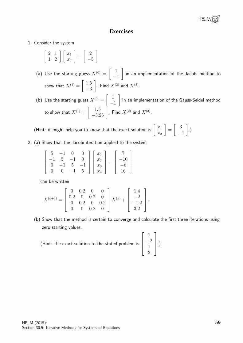
Exercises

1. Consider the system[2 11 2

] [x1

x2

]=

[2−5

]

(a) Use the starting guess X(0) =

[1−1

]in an implementation of the Jacobi method to

show that X(1) =

[1.5−3

]. Find X(2) and X(3).

(b) Use the starting guess X(0) =

[1−1

]in an implementation of the Gauss-Seidel method

to show that X(1) =

[1.5−3.25

]. Find X(2) and X(3).

(Hint: it might help you to know that the exact solution is

[x1

x2

]=

[3−4

].)

2. (a) Show that the Jacobi iteration applied to the system5 −1 0 0−1 5 −1 00 −1 5 −10 0 −1 5

x1

x2

x3

x4

=

7−10−616

can be written

X(k+1) =

0 0.2 0 00.2 0 0.2 00 0.2 0 0.20 0 0.2 0

X(k) +

1.4−2−1.23.2

.

(b) Show that the method is certain to converge and calculate the first three iterations using

zero starting values.

(Hint: the exact solution to the stated problem is

1−213

.)


59

Answers

1. (a) 2x(1)1 = 2− 1x

(0)2 = 2

and therefore x(1)1 = 1.5

2x(1)2 = −5− 1x

(0)1 = −6

which implies that x(1)2 = −3. These two values give the required entries in X(1). A

second and third iteration follow in a similar way to give

X(2) =

[2.5

−3.25

]and X(3) =

[2.625−3.75

]

(b) 2x(1)1 = 2− 1x

(0)2 = 3

and therefore x(1)1 = 1.5. This new approximation to x1 is used straight away when

finding a new approximation to x(1)2 .

2x(1)2 = −5− 1x

(1)1 = −6.5

which implies that x(1)2 = −3.25. These two values give the required entries in X(1). A

second and third iteration follow in a similar way to give

X(2) =

[2.625

−3.8125

]and X(3) =

[2.906250−3.953125

]where X(3) is given to 6 decimal places

2. (a) In this case D =

5 0 0 00 5 0 00 0 5 00 0 0 5

and therefore D−1 =

0.2 0 0 00 0.2 0 00 0 0.2 00 0 0 0.2

.

So the iteration matrix M=D−1

0 −1 0 0−1 0 −1 00 −1 0 −10 0 −1 0

=

0 0.2 0 00.2 0 0.2 00 0.2 0 0.20 0 0.2 0

and that the Jacobi iteration takes the form

X(k+1) = MX(k) +M−1

7−10−616

=

0 0.2 0 00.2 0 0.2 00 0.2 0 0.20 0 0.2 0

X(k) +

1.4−2−1.23.2

as required.


®

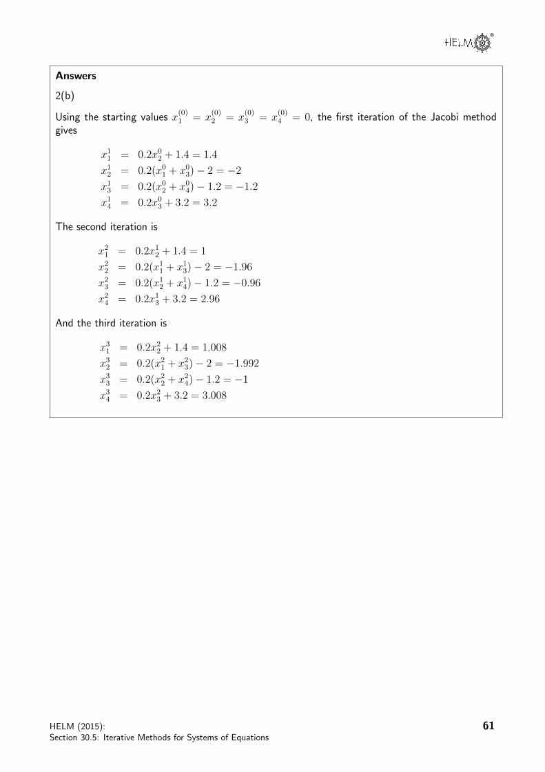
Answers

2(b)

Using the starting values x(0)1 = x

(0)2 = x

(0)3 = x

(0)4 = 0, the first iteration of the Jacobi method

gives

x11 = 0.2x0

2 + 1.4 = 1.4

x12 = 0.2(x0

1 + x03)− 2 = −2

x13 = 0.2(x0

2 + x04)− 1.2 = −1.2

x14 = 0.2x0

3 + 3.2 = 3.2

The second iteration is

x21 = 0.2x1

2 + 1.4 = 1

x22 = 0.2(x1

1 + x13)− 2 = −1.96

x23 = 0.2(x1

2 + x14)− 1.2 = −0.96

x24 = 0.2x1

3 + 3.2 = 2.96

And the third iteration is

x31 = 0.2x2

2 + 1.4 = 1.008

x32 = 0.2(x2

1 + x23)− 2 = −1.992

x33 = 0.2(x2

2 + x24)− 1.2 = −1

x34 = 0.2x2

3 + 3.2 = 3.008


61

Engineering Example 1

Detecting a train on a track

Introduction

One means of detecting trains is the ‘track circuit’ which uses current fed along the rails to detectthe presence of a train. A voltage is applied to the rails at one end of a section of track and a relay isattached across the other end, so that the relay is energised if no train is present, whereas the wheelsof a train will short circuit the relay, causing it to de-energise. Any failure in the power supply or abreakage in a wire will also cause the relay to de-energise, for the system is fail safe. Unfortunately,there is always leakage between the rails, so this arrangement is slightly complicated to analyse.

Problem in words

A 1000 m track circuit is modelled as ten sections each 100 m long. The resistance of 100 m of onerail may be taken to be 0.017 ohms, and the leakage resistance across a 100 m section taken to be30 ohms. The detecting relay and the wires to it have a resistance of 10 ohms, and the wires fromthe supply to the rail connection have a resistance of 5 ohms for the pair. The voltage applied atthe supply is 4V . See diagram below. What is the current in the relay?

4 volts

5 ohm

0.017

30oh

m

relay and wires10 ohm

i1 i2 i3 i4 i5 i6 i7 i8 i9 i10 i11ohm 0.017 ohm 0.017 ohm

30oh

m

30oh

m

30oh

m

0.017 ohm 0.017 ohm

Figure 1Mathematical statement of problem

There are many ways to apply Kirchhoff’s laws to solve this, but one which gives a simple set ofequations in a suitable form to solve is shown below. i1 is the current in the first section of rail (i.e.the one close to the supply), i2 , i3, . . . i10, the current in the successive sections of rail and i11 thecurrent in the wires to the relay. The leakage current between the first and second sections of railis i1 − i2 so that the voltage across the rails there is 30(i1 − i2) volts. The first equation belowuses this and the voltage drop in the feed wires, the next nine equations compare the voltage dropacross successive sections of track with the drop in the (two) rails, and the last equation comparesthe voltage drop across the last section with that in the relay wires.

30(i1 − i2) + (5.034)i1 = 4

30(i1 − i2) = 0.034i2 + 30(i2 − i3)

30(i2 − i3) = 0.034i2 + 30(i3 − i4)...

30(i9 − i10) = 0.034i10 + 30(i10 − i11)

30(i10 − i11) = 10i11


®

These can be reformulated in matrix form as Ai = v, where v is the 11× 1 column vector with firstentry 4 and the other entries zero, i is the column vector with entries i1, i2, . . . , i11 and A is thematrix

A =

35.034 -30 0 0 0 0 0 0 0 0 0-30 60.034 -30 0 0 0 0 0 0 0 00 -30 60.034 -30 0 0 0 0 0 0 00 0 -30 60.034 -30 0 0 0 0 0 00 0 0 -30 60.034 -30 0 0 0 0 00 0 0 0 -30 60.034 -30 0 0 0 00 0 0 0 0 -30 60.034 -30 0 0 00 0 0 0 0 0 -30 60.034 -30 0 00 0 0 0 0 0 0 -30 60.034 -30 00 0 0 0 0 0 0 0 -30 60.034 -300 0 0 0 0 0 0 0 0 -30 40

Find the current i1 in the relay when the input is 4V , by Gaussian elimination or by performing anL-U decomposition of A.

Mathematical analysis

We solve Ai = v as above, although actually we only want to know i11. Letting M be the matrix Awith the column v added at the right, as in Section 30.2, then performing Gaussian elimination onM , working to four decimal places gives

M=

35.0340 -30.0000 0 0 0 0 0 0 0 0 0 4.00000 34.3447 -30.0000 0 0 0 0 0 0 0 0 3.42520 0 33.8291 -30.0000 0 0 0 0 0 0 0 2.99190 0 0 33.4297 -30.0000 0 0 0 0 0 0 2.65320 0 0 0 33.1118 -30.0000 0 0 0 0 0 2.38100 0 0 0 0 32.8534 -30.0000 0 0 0 0 2.15720 0 0 0 0 0 32.6396 -30.0000 0 0 0 1.96980 0 0 0 0 0 0 32.4601 -30.0000 0 0 1.81050 0 0 0 0 0 0 0 32.3077 -30.0000 0 1.67330 0 0 0 0 0 0 0 0 32.1769 -30.0000 1.55380 0 0 0 0 0 0 0 0 0 12.0296 1.4487

from which we can calculate that the solution i is

i =

0.53560.49210.44920.40680.36490.32340.28220.24140.20080.16050.1204

so the current in the relay is 0.1204 amps, or 0.12 A to two decimal places.

You can alternatively solve this problem by an L-U decomposition by finding matrices L and U suchthat M = LU . Here we have


63

L =

1.0000 0 0 0 0 0 0 0 0 0 0-0.8563 1.0000 0 0 0 0 0 0 0 0 0

0 -0.8735 1.0000 0 0 0 0 0 0 0 00 0 -0.8868 1.0000 0 0 0 0 0 0 00 0 0 -0.8974 1.0000 0 0 0 0 0 00 0 0 0 -0.9060 1.0000 0 0 0 0 00 0 0 0 0 -0.9131 1.0000 0 0 0 00 0 0 0 0 0 -0.9191 1.0000 0 0 00 0 0 0 0 0 0 -0.9242 1.0000 0 00 0 0 0 0 0 0 0 -0.9286 1.0000 00 0 0 0 0 0 0 0 0 -0.9323 1.0000

and

U =

35.0340 -30.0000 0 0 0 0 0 0 0 0 00 34.3447 -30.0000 0 0 0 0 0 0 0 00 0 33.8291 -30.0000 0 0 0 0 0 0 00 0 0 33.4297 -30.0000 0 0 0 0 0 00 0 0 0 33.1118 -30.0000 0 0 0 0 00 0 0 0 0 32.8534 -30.0000 0 0 0 00 0 0 0 0 0 32.6395 -30.0000 0 0 00 0 0 0 0 0 0 32.4601 -30.0000 0 00 0 0 0 0 0 0 0 32.3076 -30.0000 00 0 0 0 0 0 0 0 0 32.1768 -30.00000 0 0 0 0 0 0 0 0 0 12.0295

Therefore Ui =

4.00003.42402.98922.65142.37832.15471.96731.80791.67051.55191.4464

and hence i =

0.53520.49170.44870.40640.36440.32300.28190.24110.20060.16030.1202

and again the current is found to be 0.12 amps.

Mathematical comment

You can try to solve the equation Ai = v by Jacobi or Gauss-Seidel iteration but in both cases it willtake very many iterations (over 200 to get four decimal places). Convergence is very slow because thenorms of the relevant matrices in the iteration are only just less than 1. Convergence is neverthelessassured because the matrix A is diagonally dominant.


Index for Workbook 30

Augmented matrix 13

Back substitution 13, 26

Conditioning 8, 41Condition number 40Convergence of iterative methods 56-58

Diagonal dominance 58

Error bonds 5

Forward substitution 25

Gaussian elimination 12-20, 62Gauss-Seidel iteration 52

Ill-conditioning 8Iterative methods 46-64

Jacobi iteration 48

Lower triangular matrix 22LU decomposition 21-33

Matrix - lower triangular 22- LU form 25- norm 34-45- upper triangular 13, 22

Norm - 1-norm 36- Euclidean 38- infinity 37

Partial pivoting 15-20Pivoting 15

Quadratic equation 6-8

Rounding - down 3- error 5- up 3

Simultaneous equations 13, 25, 46

Train on track 62

Upper triangular matrix 13, 22

Well-conditioning 8

EXERCISES10, 19, 30, 43, 59

ENGINEERING EXAMPLES1 Detecting a train on a track 62

Rounding error and conditioning, Gaussian elimination, LU ...

Documents

Transcript of Rounding error and conditioning, Gaussian elimination, LU ...